Quantitatively estimating main soil water-soluble salt ... · 372 ions content, SR method was the...

A peer-reviewed version of this preprint was published in PeerJ on 22January 2019.

View the peer-reviewed version (peerj.com/articles/6310), which is thepreferred citable publication unless you specifically need to cite this preprint.

Wang H, Chen Y, Zhang Z, Chen H, Li X, Wang M, Chai H. 2019. Quantitativelyestimating main soil water-soluble salt ions content based on Visible-nearinfrared wavelength selected using GC, SR and VIP. PeerJ 7:e6310https://doi.org/10.7717/peerj.6310

https://doi.org/10.7717/peerj.6310

https://doi.org/10.7717/peerj.6310

Quantitatively estimating main soil water-soluble salt ions

content based on Visible-near infrared wavelength selected

using GC, SR and VIP

Haifeng Wang 1, 2 , Yinwen Chen 3 , Zhitao Zhang Corresp., 1, 2 , Haorui Chen 4 , Xianwen Li 2 , Mingxiu Wang 5 ,

Hongyang Chai 2

1 Key Laboratory of Agricultural Soil and Water Engineering in Arid and Semiarid Areas, Ministry of Education, Northwest A&F University, Yangling,

Shaanxi, China2 College of Water Resources and Architectural Engineering, Northwest A&F University, Yangling, Shaanxi, China

3 Department of Foreign Languages, Northwest A&F University, Yangling, Shaanxi, China

4 Department of Irrigation and Drainage, China Institute of Water Resources and Hydropower Research, Beijing, China

5 Department of Civil and Environmental Engineering, University of California, Irvine, CA, USA

Corresponding Author: Zhitao Zhang

Email address: [email protected]

Soil salinization is the primary obstacle to the sustainable development of agriculture and

eco-environment in arid regions. The accurate inversion of the major water-soluble salt

ions in the soil using visible-near infrared (VIS-NIR) spectroscopy technique can enhance

the effectiveness of saline soil management. However, the accuracy of spectral models of

soil salt ions turns out to be affected by high dimensionality and noise information of

spectral data. This study aims to improve the model accuracy by optimizing the spectral

models based on the exploration of the sensitive spectral intervals of different salt ions. To

this end, 120 soil samples were collected from Shahaoqu Irrigation Area in Inner Mongolia,

China. After determining the raw reflectance spectrum and content of salt ions in the lab,

the spectral data were pre-treated by standard normal variable (SNV). Subsequently the

sensitive spectral intervals of each ion were selected using methods of gray correlation

(GC), stepwise regression (SR) and variable importance in projection (VIP). Finally, the

performance of both models of partial least squares regression (PLSR) and support vector

regression (SVR) was investigated on the basis of the sensitive spectral intervals. The

results indicated that the model accuracy based on the sensitive spectral intervals

selected using different analytical methods turned out to be different: VIP was the highest,

SR came next and GC was the lowest. The optimal inversion models of different ions were

different. In general, both PLSR and SVR had achieved satisfactory model accuracy, but

PLSR outperformed SVR in the forecasting effects. Great difference existed among the

optimal inversion accuracy of different ions: the predicative accuracy of Ca2+, Na+, Cl-, Mg2+

and SO42- was very high, that of CO3

2- was high and K+ was relatively lower, but HCO3- failed

to have any predicative power. These findings provide a new approach for the optimization

PeerJ Preprints | https://doi.org/10.7287/peerj.preprints.27447v1 | CC BY 4.0 Open Access | rec: 24 Dec 2018, publ: 24 Dec 2018

of the spectral model of water-soluble salt ions and improvement of its predicative

precision.


1 Quantitatively estimating main soil water-soluble salt

2 ions content based on Visible-near infrared

3 wavelength selected using GC, SR and VIP

4

5 Haifeng Wang1,2﹡, Yinwen Chen3﹡, Zhitao Zhang1,2, Haorui Chen4, Xianwen Li2, Mingxiu

6 Wang5 and Hongyang Chai2

7

8 1 Key Laboratory of Agricultural Soil and Water Engineering in Arid and Semiarid Areas,

9 Ministry of Education, Northwest A&F University, Yangling, Shaanxi, China

10 2 College of Water Resources and Architectural Engineering, Northwest A&F University,

11 Yangling, Shaanxi, China

12 3 Department of Foreign Languages, Northwest A&F University, Yangling, Shaanxi, China

13 4 Department of Irrigation and Drainage, China Institute of Water Resources and Hydropower

14 Research, Beijing, China

15 5 Department of Civil and Environmental Engineering, University of California, Irvine, CA, USA

16

17 ﹡ These authors contributed equally to this work.

18 Corresponding Author:

19 Zhitao Zhang1,2

20 No.23 Weihui Road, Yangling, Shaanxi, 712100, China

21 Email address: [email protected]

22

23

24

25

26

27

28

29

30

31

32


33

34 ABSTRACT

35 Soil salinization is the primary obstacle to the sustainable development of agriculture and eco-

36 environment in arid regions. The accurate inversion of the major water-soluble salt ions in the

37 soil using visible-near infrared (VIS-NIR) spectroscopy technique can enhance the effectiveness

38 of saline soil management. However, the accuracy of spectral models of soil salt ions turns out to

39 be affected by high dimensionality and noise information of spectral data. This study aims to

40 improve the model accuracy by optimizing the spectral models based on the exploration of the

41 sensitive spectral intervals of different salt ions. To this end, 120 soil samples were collected

42 from Shahaoqu Irrigation Area in Inner Mongolia, China. After determining the raw reflectance

43 spectrum and content of salt ions in the lab, the spectral data were pre-treated by standard normal

44 variable (SNV). Subsequently the sensitive spectral intervals of each ion were selected using

45 methods of gray correlation (GC), stepwise regression (SR) and variable importance in

46 projection (VIP). Finally, the performance of both models of partial least squares regression

47 (PLSR) and support vector regression (SVR) was investigated on the basis of the sensitive

48 spectral intervals. The results indicated that the model accuracy based on the sensitive spectral

49 intervals selected using different analytical methods turned out to be different: VIP was the

50 highest, SR came next and GC was the lowest. The optimal inversion models of different ions

51 were different. In general, both PLSR and SVR had achieved satisfactory model accuracy, but

52 PLSR outperformed SVR in the forecasting effects. Great difference existed among the optimal

53 inversion accuracy of different ions: the predicative accuracy of Ca2+, Na+, Cl-, Mg2+ and SO42-

54 was very high, that of CO32- was high and K+ was relatively lower, but HCO3

- failed to have any

55 predicative power. These findings provide a new approach for the optimization of the spectral

56 model of water-soluble salt ions and improvement of its predicative precision.

57 Introduction

58 Soil salinization, one of the most important causes of land desertification and deterioration, has

59 posed serious threat to agricultural development and sustainable utilization of natural resources

60 (Shahid & Rahman, 2011; Abbas et al. 2013). 950 million ha of saline soil worldwide has

61 become salinized (Schofield & Kirkby, 2003). Soil salinization is eroding and degenerating the

62 arable soil at the speed of 10 ha/min (Graciela & Alfred, 2009). Soil remediation and

63 management are very difficult in China because of such complex natural factors as climate,

64 terrain and geology, and human factors as unreasonable irrigation and disruption of ecological

65 balance. The total area of saline soil in China is 36 million ha (Li et al. 2014), accounting for

66 4.88% of the total area available nationwide (The National Soil Survey Office, 1998). Saline soil


67 usually has a high concentration of salt ions with a series of effects on the plants such as

68 physiological draught, ion toxicity and metabolic disorder, thus forming “salt damage” (Munns,

69 2002; Tavakkoli et al. 2011). In addition, one major cause of the inaccuracy of soil salinity

70 spectral measurement is that pure salts seldom exist in the soil because of some trace salt ion

71 elements are always fixed in soil crystals. Therefore, quick and accurate acquisition of the

72 detailed information of the various salt ions content in the soil can enhance the pertinence and

73 effectiveness of saline soil management.

74 The traditional quantitative estimation of soil salt contents usually includes such steps as field

75 soil sampling in fixed points, experiments in the laboratory and comprehensive statistical

76 analysis (Urdanoz & Aragüés, 2011). Such method is incapable of the dynamic monitoring of

77 saline soil in a large area because of its high consumption of time and energy, small number of

78 measuring points and poor representativeness (Ding & Yu, 2014). Compared with conventional

79 laboratory analysis methods, remote sensing technology has been widely used due to its rich

80 information, continuity, high precision and low cost (Ben-Dor, 2002; Viscarra Rossel et al. 2006;

81 Viscarra Rossel & Behrens, 2010; Viscarra Rossel & Webster, 2012). The various soil

82 constituents (contents of water, salt, organic matter and so forth) can be acquired conveniently

83 from remote sensing data (Gomez et al. 2008; Yu et al. 2010; Periasamy & Shanmugam, 2017).

84 Hence, with the abundant spectral reflection information within the VIS-NIR intervals of soil

85 salinity, it is feasible to improve the accuracy of soil salinization inversion (Al-Khaier, 2003;

86 Ben-Dor et al. 2009; Abbas et al. 2013).

87 The application of VIS-NIR spectral analysis technique has been proved effective in

88 improving the accuracy of quantitative estimation and eliminating the external disturbance to

89 some extent (Dehaan & Taylor, 2002; Metternicht & Zinck, 2003; Farifteh et al. 2008). The

90 univariate linear regression on the basis of soil salinity index developed for CR (continuum

91 removed) reflectance can be used as a method for soil salt content estimation (Weng et al. 2008).

92 Due to the strong correlation between soil electrical conductivity (EC) and soil salinity, EC is

93 also one of the important indicators for evaluating soil salinization degree. A variety of

94 approaches have been used to acquire the EC in the field soil, including the partial least squares

95 regression (PLSR) and multivariate adaptive regression splines (MARS) (Volkan Bilgili et al.

96 2010; Nawar et al. 2015), logarithmic model (Xiao et al. 2016a), Bootstrap-BP neural network

97 model (Wang et al. 2018d) and satellite remote sensing technology (Nawar et al. 2014; Bannari

98 et al. 2018). In addition, the differential transformation (Xia et al. 2017) and fractional derivative

99 (Wang et al. 2017; Wang et al. 2018c) can fully utilize the potential spectral information and

100 enhance model accuracy. The methods of spectral classification (Jin et al. 2015) and water

101 influence elimination (Chen et al. 2016; Peng et al. 2016; Yang & Yu, 2017) work well in

102 improving the quantitative inversion accuracy of soil salinity. Therefore, the remote sensing


103 technique is reliable to inverse the soil salinity quantitatively on different scales.

104 The quantitative analysis of VIS-NIR spectral intervals can help evaluate the content of some

105 chemical elements (Viscarra Rossel et al. 2006; Farifteh et al. 2008; Cécillon et al. 2009; Ji et al.

106 2016) due to the different characteristic absorption spectrum in soil chemical elements. Besides,

107 there exists a correlation between some principal salt ions (Na+, Cl-) and spectral reflectance

108 (Jiang et al. 2017). Therefore, VIS-NIR spectroscopy technique can be used to obtain the

109 contents of the soil salt ions to a certain extent. The spectral response characteristics of mid-

110 infrared (MIR) spectroscopy are better than those of VIS-NIR spectroscopy in predicting soil

111 salinity information, the latter has high predicting accuracy of the total salts content, HCO3-,

112 SO42- and Ca2+, followed by Mg2+, Cl- and Na+ (Peng et al. 2016). The spectral models have

113 satisfactory prediction of the SAR (sodium absorption ratio) of soil salinization evaluation

114 parameter, which is composed of the contents of Ca2+, Mg2+ and Na+ (Xiao et al. 2016b). Qu et

115 al. (2009) found that the contents of the total salt, SO42-, pH and K++Na+ have a higher inversion

116 accuracy using spectral data to create PLSR model. The different pretreatment of the different

117 ion models varies by creating and analyzing PLSR model that demonstrates relatively good

118 predictive effects like ion contents of Ca2+, Mg2+, SO42-, Cl-, and HCO3

- (Dai et al. 2015).

119 Overall, PLSR is a frequently used and robust linear model for quantitative research because it

120 has inference capabilities which are useful to model a probable linear relationship between the

121 reflectance spectra and the salt ions content in soil. However, the non-uniform data and non-

122 linear reflectance in spectral information of some soil chemical elements lead to the reduction in

123 model accuracy (Viscarra Rossel & Behrens, 2010; Nawar et al. 2015). In particular, support

124 vector regressions (SVR) based on kernel-based learning methods has the ability to handle

125 nonlinear analysis case with high model accuracy (Vapnik, 1995; Peng et al. 2016; Hong et al.

126 2018b). Over the past several decades, the use of SVR for classification and regression has been

127 extensively applied in soil VIS-NIR spectroscopy (Ben-Dor, 2002; Xiao et al. 2016b; Hong et al.

128 2018a). Moreover, the SVR model works well in estimating the contents of K+, Na+, Ca2+ and

129 SO42- in the soil (Wang et al. 2018a). Thus, the correct way of modeling helps to guarantee the

130 model accuracy (Farifteh et al. 2007).

131 Many researches focused on the inversion of soil salinity using spectral information.

132 Nevertheless, little research has explored the eight water-soluble salt ions (K+, Ca2+, Na+, Mg2+,

133 Cl-, SO42-, HCO3

- and CO32-) using spectral information in the soil. The model fitting of ions and

134 spectral information still needs improving (Farifteh et al. 2008; Peng et al. 2016). Apart from the

135 suitable multivariate statistical analysis method that can partly improve the inversion effects,

136 reduction of redundant information is another identified approach to further optimize the model

137 (Bannari et al. 2018; Stenberg et al. 2010). Plenty of studies have demonstrated that spectral

138 variable selection methods can not only reduce the complexity of calibration models, but also


139 improve the model predictive performance (Hong et al. 2018a). To select the optimal spectral

140 variable subset, scholars have investigated varied methods such as gray correlation (GC) (Li et al.

141 2016; Wang et al. 2018b), stepwise regression (SR) (Zhang et al. 2018) and variable importance

142 in projection (VIP) (Qi et al. 2017), and have achieved satisfactory effects. In addition, all the

143 three methods have been widely applied in many studies, such as plant physiology, food

144 engineering, mathematical statistics (Oussama et al., 2012; Maimaitiyiming et al. 2017; Liu et al.

145 2015). However, few studies have concentrated on the use of variable selection algorithms in the

146 inversion of soil salt ions.

147 This study aims to: (1) build the optimal model of soil salt ions using VIS–NIR spectroscopy

148 technique; (2) compare the models based on the sensitive spectral ranges selected using GC, SR

149 and VIP methods for different soil ions; (3) compare the performance of PLSR and SVR models,

150 and identify the optimal models for different ions.

151 MATERIALS AND METHODS

152 Study area

153 Hetao Irrigation District (HID), with Yin Mountains at its north, the Yellow River at its south,

154 Ulanbuh Desert at its west and Baotou at its east, lies in Bayannur League, Inner Mongolia,

155 China. It consists of irrigation areas of Ulan Buh, Jiefangzha, Yongji, Yichang and Urat, and it is

156 China’s largest irrigation district with a total size of 5740 km2 (Yu et al. 2010). In addition, HID

157 is an important production base of cereal and oil plants in China with major crops of wheat, corn

158 and sunflower. Shahaoqu Irrigation Area (SIA), a typical region of saline soil in HID, was

159 chosen as the study area. SIA (10705～10710E, 4052～4100N) is located in the central

160 east of Jiefangzha Irrigation Area. SIA belongs to typical continental climate, having hot

161 summers, chilly winters, rare precipitation and strong evaporation. Its mean annual temperature,

162 precipitation, potential evaporation is about 7.1℃, 155 mm and 2000 mm, respectively.

163 Physiographically, the mean elevation and slope of SIA are about 1030 m and 1/10000,

164 respectively. According to the World Reference Base for Soil Resources (WRB), the local soil

165 texture is mainly silty clay loam with varying degrees of saline soil. Over the years, due to its

166 gentle terrain slope, poor groundwater runoff, intense land surface evaporation and irrational

167 farming activities, about 60% of the land within the district has been affected by various degree

168 of salinization, which seriously restricted the agricultural development (Wu et al. 2008; Gao et al.

169 2015).

170 Sample collection and chemical analysis

171 The Hetao irrigation district administration gave field permit approval to us (NO.

172 2017YFC0403302). To ensure the representativeness of soil samples, the samples were


173 randomly gathered from a total of 120 sampling units on a grid of 16 m×16 m (because the

174 spatial resolution of GF-1 satellite imagery is 16 m) in the study area during October 12～22,

175 2017 (Fig. 1). In each unit, approximately 0.5 kg of topsoil (0-5 cm) was collected at four

176 randomly selected sampling sites and then mixed thoroughly to obtain a representative sample.

177 Overall, a total of 120 soil samples were acquired, and each sample was stored in a plastic bag,

178 labeled and sealed. A portable global position system (GPS) was used to determine the

179 coordinates of sampling points. Subsequently, the soil samples were transported to the lab to

180 receive a series of such treatments as sufficient natural air-drying for two weeks and rubbing

181 through a 2 mm sieve to exclude small stones and other impurities. Each sample was divided into

182 two subsamples to be used for spectra collection and physiochemical analysis.

183 Each 50 g of soil sample was put into a respective flask, and 250 ml of distilled water (the

184 ratio of water to soil is 5:1) were added into each flask. The water-soluble ion contents were

185 measured in the filtrate obtained from full soaking, oscillation and filtration (Aboukila & Norton,

186 2017). Ca2+ and Mg2+ were measured using EDTA titration, Na+ and K+ flame photometry, CO32-

187 and HCO3- double indicator-neutralization titration, Cl- silver nitrate titration, and SO4

2- EDTA

188 indirect complexometry (Bao, 2000). The content of CO32- was too low (approximately 0) in

189 some soil samples because CO32- is liable to integrate with Ca2+ and Mg2+ as sediment in a weak

190 alkaline solution (Table 1). Coefficient of variation (CV) reflects the degree of discreteness, and

191 a positive correlation exists in two variables. The high CV helps to build a robust model (Dai et

192 al. 2015). The grading of CV showed a wide range of variation among different ions, among

193 which the ion contents of K+, Na+ and SO42- are over 100%, showing a strong variability, and

194 those of CO32-, Cl-, Ca2+, Mg2+ and HCO3

- are between 10% and 100%, having a moderate

195 variability.

196 Laboratory spectral measurements and pretreatments

197 The soil samples were put into black vessels with a diameter of 10 cm and depth of 2 cm for

198 spectral data collection and the surfaces were smoothed with a straightedge in the laboratory.

199 The spectral data of the soil samples were measured using ASD (Analytical Spectral Devices,

200 Inc., Boulder, CO, USA) FieldSpec®3 spectrometer with spectral range from 350-2500 nm. This

201 instrument is equipped with two sensors whose spectral resolutions are 1.4 nm and 2 nm, for the

202 region of 350-1000 nm and 1000-2500 nm, respectively. The spectral data was measured in a

203 dark room with the light sources which have halogen lamps of 50 W, 50 cm from the sample soil

204 surfaces, and 30° incident angle to reduce the effects of external factors to the minimum. The

205 field angle of fiber-optics probe is 5°, and it is 15 cm from the sample soil surface. The light

206 source and spectrometer had been fully preheated, and the spectrometer had been corrected with

207 a standardized white panel (99% reflectance) prior to each measurement to reduce measurement


208 error. Each sample soil was measured in four directions (3 turns, each is 90°), the spectrum was

209 collected five times in each direction, and altogether there were 20 curves of the spectrum (Hong

210 et al. 2018b). These curves were used as the raw spectral reflectance (Rraw) after having the

211 arithmetic mean in ViewSpecPro software version 6.0. The gaps of the spectral curves near 1000

212 nm and 1800 nm were corrected using Splice Correction function (Xiao et al., 2016a).

213 The fluctuation would affect the accuracy of subsequent modeling because of such disturbance

214 as the external environment, instrument noise and random error in spectral data collection. In

215 general, a series of effective pretreatment, including smoothing, resampling and transformation

216 etc., can eliminate the external noise to some degree, and then enhance the spectral

217 characteristics (Ding et al. 2018). Therefore, it is necessary to pretreat Rraw in the following steps.

218 i) The marginal wavelength (350-399 nm and 2401-2500 nm) of higher noise in each soil sample

219 was removed, then remaining spectrum data was smoothed with filter method (window size is 5

220 and polynomial order is 2) using Savitzky-Golay (SG) (Savitzky & Golay, 1964) via Origin Pro

221 software version 2017SR2. ii) The spectral data between 400 and 2400 nm was resampled with a

222 10 nm of samplee interval to keep the spectral features and remove redundant information (Xu et

223 al. 2016). A new spectral curve consisting of 200 wave bands was obtained. iii) The precise Rraw-

224 SNV was obtained by using standard normal variable (SNV) to eliminate the effects of soil particle

225 size, surface scattering and baseline shift on the spectrum data (Xiao et al., 2016b; Barnes et al.,

226 1989). The spectral curves of Rraw and Rraw-SNV are shown in Fig. 2A and 2B. Notably,

227 comparison indicated that the spectral curve in Fig. 2B was much smoother than that in Fig. 2A,

228 which made for the subsequent modeling.

229 Gray correlation (GC)

230 The GC, as one grey system theory, seeks the primary and secondary relations and analyzes the

231 different effects of all the factors in a system (Deng, 1982; Li et al. 2016). Its calculation process

232 is as follows: the reference sequence is , the comparative sequence is 0 0 , 1, 2, ,X x t t n

233 , and the formula of the gray correlation degree (GCD) between , 1, 2, ,i iX x t t n 0X

234 and is iX

235 (1) 0

1

1GCD = ,

n

i

t

x t x tn

236 where 0 0

0

0 0

min min ( ) ( ) max max ( ) ( ), =

( ) ( ) max max ( ) ( )

i ii t i t

i

i ii t

x t x t x t x tx t x t

x t x t x t x t

237 is the distinguishing coefficient within . was set as 0.1 in this paper. 0 1，


238 The inconsistent dimension between the spectral data and the contents of different ions has

239 some effects on the data analysis. Therefore, normalizing the spectral data preprocessing method

240 can reduce these disadvantageous effects (Liu et al. 2015; Wang et al. 2018b). In this paper, the

241 larger the GCD of a certain band is, the closer relation the band and the ion content has, and vice

242 versa.

243 Variable importance in projection (VIP)

244 The VIP is a variable selection method based on PLSR (Oussama et al., 2012). The explanatory

245 power of the independent variables to the dependent variables is achieved by calculating the VIP

246 score. The independent variables are sequenced according to the explanatory power (Qi et al.

247 2017). The VIP score for the j-th variable is given as:

248 （2）

2

1

SSY W

VIPSSY

F

f jf

f

jtotal

p

F

249 Where p is the number of independent variables; m is the total number of components; SSYf is

250 the sum of squares of explained variance for the f-th component and p the number of independent

251 variables. SSYtotal is the total sum of squares explained of the dependent variable, and F is the

252 total number of components. gives the importance of the j-th variable in each f-th 2Wjf

253 component. The higher value VIPj has, the stronger explanatory power the independent variable

254 has over the dependent variable. The VIP scores of independent variables have been recognized

255 as a useful measure to identify important wavelengths when the score is more than 1 (Wold et al.

256 2001; Maimaitiyiming et al. 2017).

257 Model construction and validation

258 Two thirds of the samples were used for modeling (n = 80) and one third for validation (n = 40)

259 using Kennard-Stone (K-S) to calculate the Euclidian distance among different samples to ensure

260 the statistical characteristics of modeling and the validation datasets resembled that of the whole

261 sample set (Kennard & Stone, 1969).

262 The PLSR and SVR models were applied to the quantitative inversion of different water-

263 soluble salt ion contents in the saline soil in this paper. The PLSR model is a new stoichiometric

264 statistical model. Compared with the traditional multivariate least squares regression (MLSR),

265 PLSR can overcome the multicollinearity among the variables, reduce the dimension, synthesize

266 and filter the information, extract the aggregate variables with the strongest explanatory power in

267 the system, and exclude the noise with no explanatory power (Wold et al. 2001). The optimal

268 fitting model was built using the number of optimal principal components through full cross

269 validation. SVR model is a new machine learning method based on the principle of structural

270 risk minimization provided by the statistical learning theory. This model is characterized by its


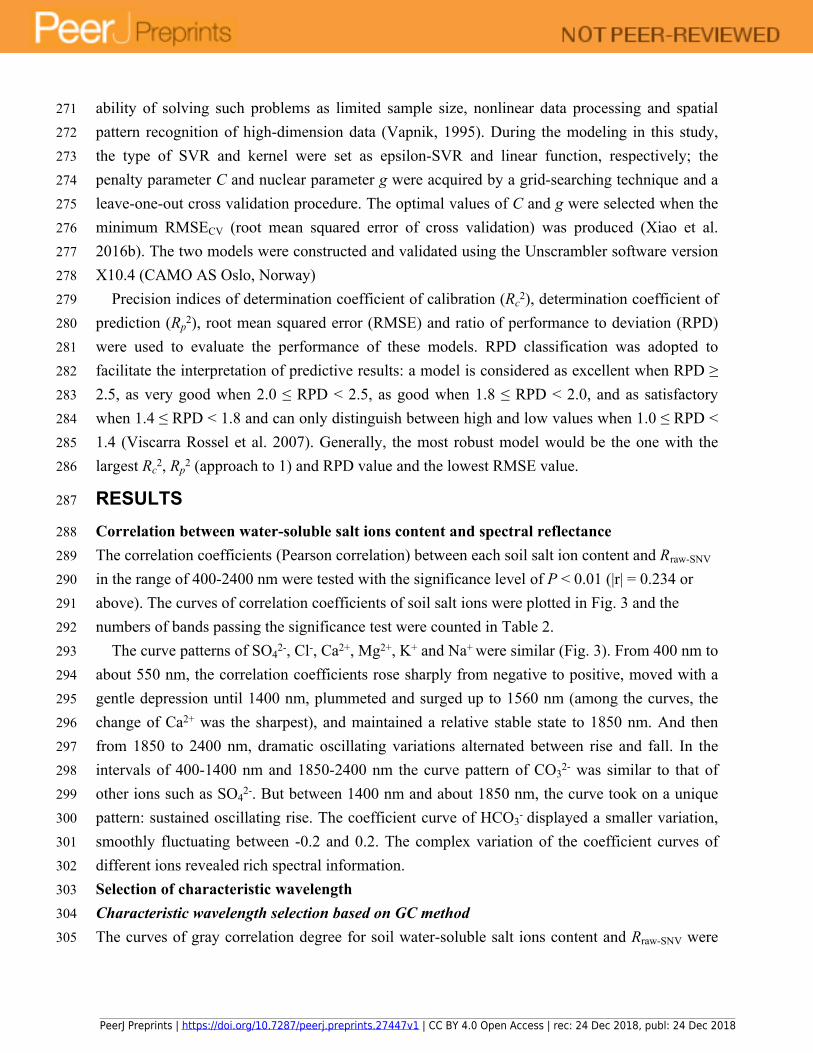
271 ability of solving such problems as limited sample size, nonlinear data processing and spatial

272 pattern recognition of high-dimension data (Vapnik, 1995). During the modeling in this study,

273 the type of SVR and kernel were set as epsilon-SVR and linear function, respectively; the

274 penalty parameter C and nuclear parameter g were acquired by a grid-searching technique and a

275 leave-one-out cross validation procedure. The optimal values of C and g were selected when the

276 minimum RMSECV (root mean squared error of cross validation) was produced (Xiao et al.

277 2016b). The two models were constructed and validated using the Unscrambler software version

278 X10.4 (CAMO AS Oslo, Norway)

279 Precision indices of determination coefficient of calibration (Rc2), determination coefficient of

280 prediction (Rp2), root mean squared error (RMSE) and ratio of performance to deviation (RPD)

281 were used to evaluate the performance of these models. RPD classification was adopted to

282 facilitate the interpretation of predictive results: a model is considered as excellent when RPD ≥

283 2.5, as very good when 2.0 ≤ RPD < 2.5, as good when 1.8 ≤ RPD < 2.0, and as satisfactory

284 when 1.4 ≤ RPD < 1.8 and can only distinguish between high and low values when 1.0 ≤ RPD <

285 1.4 (Viscarra Rossel et al. 2007). Generally, the most robust model would be the one with the

286 largest Rc2, Rp

2 (approach to 1) and RPD value and the lowest RMSE value.

287 RESULTS

288 Correlation between water-soluble salt ions content and spectral reflectance

289 The correlation coefficients (Pearson correlation) between each soil salt ion content and Rraw-SNV

290 in the range of 400-2400 nm were tested with the significance level of P < 0.01 (|r| = 0.234 or

291 above). The curves of correlation coefficients of soil salt ions were plotted in Fig. 3 and the

292 numbers of bands passing the significance test were counted in Table 2.

293 The curve patterns of SO42-, Cl-, Ca2+, Mg2+, K+ and Na+ were similar (Fig. 3). From 400 nm to

294 about 550 nm, the correlation coefficients rose sharply from negative to positive, moved with a

295 gentle depression until 1400 nm, plummeted and surged up to 1560 nm (among the curves, the

296 change of Ca2+ was the sharpest), and maintained a relative stable state to 1850 nm. And then

297 from 1850 to 2400 nm, dramatic oscillating variations alternated between rise and fall. In the

298 intervals of 400-1400 nm and 1850-2400 nm the curve pattern of CO32- was similar to that of

299 other ions such as SO42-. But between 1400 nm and about 1850 nm, the curve took on a unique

300 pattern: sustained oscillating rise. The coefficient curve of HCO3- displayed a smaller variation,

301 smoothly fluctuating between -0.2 and 0.2. The complex variation of the coefficient curves of

302 different ions revealed rich spectral information.

303 Selection of characteristic wavelength

304 Characteristic wavelength selection based on GC method

305 The curves of gray correlation degree for soil water-soluble salt ions content and Rraw-SNV were


306 shown in Fig. 4. The correlation coefficient curves of the seven ions except CO32- resembled

307 those of the GCD of the Rraw-SNV. Generally, the curves exhibited patterns of “oscillatory rise,

308 fluctuation, rapid rise and fall, and oscillatory fluctuation”. The gray correlation curves of CO32-

309 followed a pattern of “ascending, plummeting, and smooth transition”. The analysis of the GC

310 curve amplitude showed the amplitudes of Cl-, Mg2+ and Ca2+ were relatively large, and those of

311 Na+, SO42-, K+ and HCO3

- were relatively small, and that of CO32- was relatively gentle.

312 The order of the maximal GCD was: Cl- (0.561) > Mg2+ (0.559) > Ca2+ (0.551) > Na+ (0.508)

313 > SO42- (0.494) > K+ (0.470) > HCO3

- (0.465) > CO32- (0.416). To ensure that each salt ion had

314 sensitive bands as far as possible, the GCD threshold value was set as 0.40 to select the

315 wavelength. The sensitive band was counted through gray correlation method (Table 3). The

316 numbers of sensitive bands of different ions could be sequenced from the largest to the smallest

317 as follows: Mg2+ (110) > HCO3- (105) > Cl- (101) > Ca2+ (53) > Na+ (36) > SO4

2- (21) > K+ (15)

318 > CO32- (14). Therefore, the orders of sensitive band numbers and maximal GCD values had

319 great difference. Furthermore, the band intervals corresponding to the maximum GCD of

320 different salt ions were as follows: CO32- was near-infrared between 1740 and 1750 nm, HCO3

-

321 was green light between 560 and 570 nm, and the rest of six ions were near-infrared between

322 1650 and 1660 nm.

323 Characteristic wavelength selection based on SR method

324 Feature band intervals were selected by stepwise regression method in SPSS software version

325 23.0 (IBM, Chicago, USA), and the significance levels of variables acceptance and rejection

326 were set at 0.10 and 0.15 (Zhang et al. 2018). The parameter indexes of feature band intervals

327 selection were shown in Table 4 by stepwise regression method at maximum adjusted R2.

328 Great difference existed among the optimal SR models of different ions, and the numbers of

329 band intervals accepted by the model range from 3 to 8 (Table 4). The SR model fitted well with

330 the adjusted R2 greater than 0.8 when the number of selected independent variables was

331 considered. Meanwhile, SR model of each ion was statistically significant (p<0.001). Therefore,

332 the band intervals selected by the SR models were used as the independent variables of PLSR

333 and SVR models.

334 Characteristic wavelength selection based on VIP method

335 Curves of VIP scores of soil water-soluble salt ions content and Rraw-SNV were shown in Fig. 5.

336 Max VIP scores and band intervals obtained from VIP method of soil water-soluble salt ions

337 content and Rraw-SNV were shown in Table 5.

338 The curves patterns of seven ions were similar except HCO3- (Fig. 5). These curves exhibited

339 violent oscillation in the intervals of 400-800 nm and 1900-2400 nm, gentle transition between

340 800 nm and around 1400 nm, and fluctuant rise from 1400 to 1900 nm. In contrast, the curve of

341 HCO3- showed oscillatory rise from 400 to 1400 nm, a “U” shaped motion from 1400 to 1900


342 nm or so, and a rapid fall and oscillation to 2400 nm. The numbers of sensitive bands based on

343 VIP method displayed the following sequence: Cl- (85) > Na+ (83) > HCO3- (79) > SO4

2- (74) >

344 Mg2+ (69) = Ca2+ (69) = K+ (69) > CO32- (67). The sequence of the maximal VIP scores was

345 HCO3- (2.37) > CO3

2- (2.01) > Ca2+ (1.97) > SO42- (1.74) > K+ (1.73) > Na+ (1.55) > Mg2+ (1.49)

346 > Cl- (1.42). The spectral interval of the maximal VIP scores of Cl- was from 560 to 570 nm,

347 Ca2+, CO32- and HCO3

- were concentrated between 1410 and 1450 nm; and K+, Mg2+, Na+ and

348 SO42- were from 1870 to1890 nm.

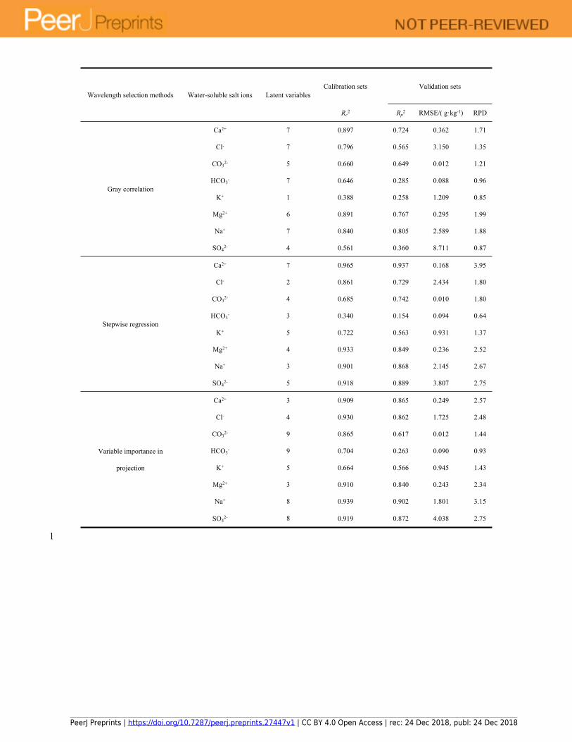
349 Construction and analysis of PLSR model

350 The sensitive bands were obtained using different band selection methods of GC, SR and VIP to

351 build PLSR model. The results of PLSR model were shown in Table 6.

352 The models of the six ions Ca2+, Cl-, CO32-, Mg2+, Na+ and SO4

2- performed well using VIP

353 method (Rc2 is close to 1). The models based on the bands of Ca2+, Cl-, Mg2+, Na+ and SO4

2-

354 selected using SR method displayed good fitting effect, and those of Ca2+, Mg2+ and Na+ using

355 GC method exhibited good fitting effect.

356 In terms of verification accuracy, VIP method had excellent prediction of Ca2+, Na+, SO42-, SR

357 method had excellent prediction of Ca2+, Mg2+, Na+, SO42- (the RPD of Ca2+ was up to 3.95), and

358 GC method did not show strong prediction power over any ions. On the contrary, all the three

359 models demonstrated poor forecasting power over HCO3-. The RPDs of SR-HCO3

- and VIP-

360 HCO3- were 0.64 and 0.93 respectively. Therefore, VIP method had the best modeling effect and

361 SR method had the best forecasting effect, and GC method had poor modeling and forecasting

362 effects on the salt ions inversion in the PLSR model.

363 Construction and analysis of SVR model

364 The sensitive bands were obtained by using different band selection methods of GC, SR and VIP

365 to build SVR model. The results of SVR model were shown in Table 7.

366 The modeling accuracy of SVR model was similar to that of PLSR model. But the verification

367 accuracy of ions was different between the two models. VIP method had the excellent prediction

368 of Ca2+, Cl-, Mg2+, Na+, SR method had the excellent prediction of Ca2+, Mg2+, Na+, SO42-, and

369 GC method did not show strong prediction power over any ions. The prediction results of Ca2+

370 were the best: the RPD of VIP and SR models were 3.93 and 3.97, respectively. Overall, in the

371 SVR model, VIP method exhibited the best performance for modeling and predicting the salt

372 ions content, SR method was the second, and GC method was relatively poorer.

373 DISCUSSION

374 Comparison among the results of different salt ions content in estimating

375 The optimal band selection method varied in some degree from the optimal modeling method

376 (Table 6 and 7). The comparison was made between the measured value and the estimated value


377 of all the ions concerned under the optimal model (Fig. 6). The sequence of the forecasting

378 power of the ions was Ca2+ > Na+ > Cl- > Mg2+ > SO42- > CO3

2- > K+ > HCO3-, and it was the

379 same as that of the modeling power.

380 Obviously, the verification result showed that most data points of the five ions, Ca2+, Na+, Cl-,

381 Mg2+ and SO42-, were concentrated near line 1:1. The optimal models of these five ions had very

382 strong predicative power with the RPD above 2.5 (Tables 6 and 7). Compared with the previous

383 researches, model prediction effects of K+ and Na+ (Qu et al. 2009); Ca2+, Na+ and Mg2+

384 (Viscarra Rossel & Webster, 2012); SO42-, HCO3

-, Ca2+, Cl-, Mg2+ and SO42- (Dai et al. 2015);

385 HCO3-, Ca2+ and SO4

2- (Peng et al. 2016); K+, Na+, Ca2+ and SO42- (Wang et al., 2018a) were

386 satisfactory. Although the results of this study are not exactly the same as these previous

387 researches, it still shows the rationality own to some extent. In addition, this result shows that

388 band selection has realized the goal of removing the irrelevant information, and plays a major

389 role in improving the inversion accuracy of salt ions.

390 In Figure 6, the data points of CO32- and K+ were relatively dispersed in the verification result.

391 The CO32- had a relatively good predictive power (RPD = 1.80) and the K+ had a normal

392 predictive power (RPD = 1.43). Notably, HCO3- had no predicative power (RPD = 0.96) because

393 the slope were under the 1:1 line and the data points were most discrete (Figs. 6D). The

394 predicting effect of HCO3- was different from that of Peng et al. (2016) and Dai et al. (2015), but

395 similar to that of Wang et al. (2018a). The cause of this result needs to be further studied. Overall,

396 it is vital to make some efforts to improve the robustness and accuracy of these ion models. Xiao

397 et al. (2016b) failed to predict Na+, Mg2+ and Ca2+, but applied the SVR model to forecasting

398 SAR after the SNV transformation and the performance was satisfactory (RPD = 2.13).

399 Analogously, first derivative reflectance (FDR) index was calculated to effectively predict SAR

400 by Xiao et al. (2016a). In addition, Viscarra Rossel & Webster (2012) forecasted the content of

401 Na+ after logarithmic pretreatment with VIS-NIR spectral technique (RPD = 2.10). Thus, salt ion

402 indexes construction and variable transformation processing are helpful approaches to improve

403 the correlation with the spectra so as to establish satisfactory models.

404 A little difference existed in the applicability between PLSR and SVR models on inversing the

405 content of ions. Both methods could produce satisfactory results in conformity with that of Peng

406 et al. (2016). In addition, the optimal inversion models and prediction models for each ion were

407 different: SR-PLSR model and SR-SVR model for Ca2+, VIP-SVR model and SR-PLSR model

408 for CO32-, SR-PLSR model and VIP-PLSR model for K+, VIP-PLSR model and GC-PLSR

409 model for HCO3- , respectively. Among them, the performance of the optimal inversion model of

410 Ca2+ resembled that of the prediction model. The results suggested that the ion models with

411 poorer performance frequently demonstrated uncertainty in the inversion process (Peng et al.

412 2016). Generally, as the major water-soluble ion components in the two highly soluble salts of


413 sodium and kali, Na+ and K+ exhibit great difference in the spectral characterization degree (Dai

414 et al. 2015). Therefore, the spectral characters of water-soluble salt ions are not necessarily

415 determined by the number of dissociative ions, so more pertinent experiments and analysis

416 should be conducted to explore the response mechanism.

417 Correlation analysis and inversion performance

418 The raw spectral reflectance curve of each soil sample presented distinct shapes (Fig. 2A). One

419 of the prime reasons for this phenomenon is that the absorption features in these soil samples

420 were related to soil salt crystal contents and types, as well as various chemical bonds (e.g., C-H,

421 O-H, N-H). The results were in accordance with those in previous studies (Viscarra Rossel et al.

422 2006; Viscarra Rossel & Webster, 2012; Dai et al. 2015; Peng et al. 2016; Wang et al. 2018a),

423 which demonstrated that soil VIS-NIR spectra could be used to determine part of soil salt ions

424 contents in some degree.

425 Traditionally, correlation analysis helps reveal the relationships between soil salt ions content

426 and VIS-NIR spectra, and it indicates modeling effects to some degree (Weng et al. 2008). In the

427 current research, the number of the significant bands of different ions could be sequenced from

428 the largest to the smallest as follows: Cl- (96%) > Ca2+ (95%) > Mg2+ (93%) > Na+ (90.5%) > K+

429 (89%) = SO42- (89%) > CO3

2- (73%) > HCO3- (0.5%), the correlation coefficients of different

430 ions ranged from the largest to the smallest as: Cl- (-0.882) > Ca2+ (-0.877) > Mg2+ (-0.848) >

431 Na+ (-0.752) > SO42- (0.749) > K+ (0.630) > CO3

2- (0.552) > HCO3- (0.235) (Table 2). Thereby,

432 five ions (Cl-, Ca2+, Mg2+, Na+ and SO42-) had more significant relationship with reflectance

433 spectra. Although there were some differences between forecasting power ranking and

434 correlation ranking, the optimal models of these five ions had the excellent predictive results (Fig.

435 6). Nevertheless, the other three ions (K+, CO32- and HCO3

-) had weak correlations and

436 unsatisfactory predictive power. In particular, HCO3- had only one significant band and the worst

437 prediction effects. But in most cases, the sensitive band numbers of HCO3- were not the least in

438 comparing the results of the three wavelength selection methods (Tables 3-5). Thus, we

439 conjecture that the different calculation mechanisms cause a certain inconsistency between

440 modeling performance and sensitivity. In addition, the optimal method of finding out their

441 responding spectrum varies from one ion to another in the soil. In future study, it is practically

442 significant to adopt various methods to select the optimal bands in the inversion of soil ions.

443 Effects of wavelength selection on estimation models

444 The massive complex spectra often contain a large amount of redundant information irrelevant to

445 the ions contents. The selection of feature spectra is hence a critical step to create a robust model.

446 From Tables 3-5, we could see the great difference exist in the number of wavelength selected

447 with the three methods: VIP method had the largest number of wavelengths (34.5%～42.5%),

448 SR method had the smallest number of wavelengths (1.5%～4%) and number of wavelengths


449 (7%～55%) varied greatly by GC method.

450 Our experiment with three wavelength selection methods also indicated that different methods

451 yielded different results. Among the three methods, the VIP method produced the best results,

452 followed by SR method, while the GC method performed least ideally. We argue that the GC

453 method is not necessarily an inappropriate method as some results are still acceptable. However,

454 GC method could distinguish the primary relationships among the factors in the system by

455 calculating and comparing GCD (Deng, 1982; Liu et al. 2015). In the field of spectral analysis,

456 the application of GC method could better identify sensitive spectral indices, select sensitive

457 bands and optimize inversion model (Li et al. 2016). On the other hand, Wang et al (2018b) used

458 GC method to extract the feature bands of soil organic matter content to construct the model with

459 stronger generalization capability. Therefore, the soil compositions have a strong impact on the

460 performance of spectral model. This conclusion is consistent with previous research results

461 (Viscarra Rossel et al. 2006; Viscarra Rossel & Webster, 2012; Xiao et al. 2016b). The VIP

462 values were calculated with VIP method, in the process of PLSR analysis to further evaluate the

463 significance of each wavelength for model prediction (Wold et al. 2001; Maimaitiyiming et al.

464 2017; Qi et al. 2017). VIP method often produces the best results in the modeling set because it

465 can distinguish between useful information and inevitable noises in the set. Oussama et al. (2012)

466 adopted this method to reduce almost 75% of the total data set for a simplified model of high

467 accuracy. Additionally, as a simplified regression linear model, SR method not only preserves

468 significant bands but also solves multicollinearity problems effectively (Xiao et al. 2016a; Xiao

469 et al. 2016b). It has great optimization effect on model complexity by adjusting the significance

470 level of selected and excluded variables (Zhang et al. 2018). Compared with the selection results

471 with VIP method, SR method could be used to extract fewer bands to establish ions (except for

472 K+, CO32- and HCO3

-) forecasting models with RPD above 1.80. Therefore, it is meaningful to

473 make further simplification of the model while ensuring its accuracy.

474 Research limitations

475 This study clearly demonstrated that VIS-NIR spectral analysis technique is an effective method

476 to detect salt ions content of salinity soil in the irrigated district. In terms of extracting feature

477 wavelengths to estimate ions content, our work provides a comprehensive comparison and

478 evaluation approaches. Such endeavor is critically and practically important to further enhance

479 the model performance of the soil salt ions. The application of machine learning algorithms with

480 strong applicability to solve nonlinear relationship between variables, such as Ant Colony

481 Optimization-interval Partial Least Square (ACO-iPLS), Recursive Feature Elimination based on

482 Support Vector Machine (RF-SVM), and Random Forest (RF) has been proved to be a useful

483 approach to obtain the effective information of soil organic matter (Ding et al. 2018). To further

484 improve the prediction accuracy, the more machine learning algorithms should be applied to the


485 analysis of sensitive spectral regions and the construction of stable models in future study. In

486 addition, the application of multi-source remote sensing platforms such as Landsat, GaoFen-5,

487 Hyperion and unmanned aerial vehicle (UAV) in soil salt ions estimation has not been

488 investigated. Therefore, further research should focus on the possible combination of multiple

489 approaches and remote sensing data at different scales to estimate soil salt ions content.

490 CONCLUSIONS

491 This study investigated the feasibility of estimating soil water-soluble salt ions content via VIS-

492 NIR spectral model. Different methods were applied to the selection of response bands interval

493 to construct robust inversion models. Among them, VIP method could select larger number of

494 wavebands with the highest accuracy, SR method could select the smallest number of wavebands

495 with good accuracy. However, the number of wavebands obtained using GC method varied

496 greatly with poor accuracy. The PLSR and SVR models achieved good effects on the modeling

497 and forecasting of most ions content. Moreover, the PLSR model was slightly more than the

498 SVR model in terms of the number of ion models with good predictive effects (RPD over 2.0).

499 The models of Ca2+, Na+, Cl-, Mg2+ and SO42- displayed the highest prediction accuracy, and the

500 RPDs were 3.97, 3.15, 2.98 and 2.75, respectively, while those of other ions were poor. Overall,

501 the best wavelength selection methods, models and inversion results of soil salt ions were

502 different. In the future, the combination of band selection methods and spectral model will have

503 a great potential for predicting some soil salt ions content in the salinization area. Such an

504 approach can be utilized to assist decision makers toward the determination of soil salinization

505 levels.

506 ACKNOWLEDGEMENTS

507 The authors want to thank A.P. Junying Chen for her help in language standardization of this

508 manuscript and providing helpful suggestions. We are especially grateful to the reviewers and

509 editors for appraising our manuscript and for offering instructive comments.

510 REFERENCE

511 Abbas A, Khan S, Hussain N, Hanjra MA, Akbar S. 2013. Characterizing soil salinity in

512 irrigated agriculture using a remote sensing approach. Physics and Chemistry of the Earth

513 55-57:43-52. DOI 10.1016/j.pce.2010.12.004

514 Aboukila EF, Norton JB. 2017. Estimation of saturated soil paste salinity from soil-water

515 extracts. Soil Science 182:107-113. DOI 10.1097/SS.0000000000000197

516 Al-Khaier F. 2003. Soil salinity detection using satellite remote sensing. Michigan

517 Technological University.

518 Bannari A, El-Battay A, Bannari R, Rhinane H. 2018. Sentinel-MSI VNIR and SWIR bands


519 sensitivity analysis for soil salinity discrimination in an arid landscape. Remote Sensing

520 10:855. DOI 10.3390/rs10060855

521 Bao S. 2000. Soil and agricultural chemistry analysis. Beijing: China Agriculture Press. (in

522 Chinese).

523 Barnes RJ, Dhanoa MS, Lister SJ. 1989. Standard normal variate transformation and de-

524 trending of near-infrared diffuse reflectance spectra. Applied Spectroscopy 43:772-777. DOI

525 10.1366/0003702894202201

526 Ben-Dor E. 2002. Quantitative remote sensing of soil properties. Advances in Agronomy 75:173-

527 243. DOI 10.1016/S0065-2113(02)75005-0

528 Ben-Dor E, Chabrillat S, Demattê JAM, Taylor GR, Hill J, Whiting ML, Sommer S. 2009.

529 Using imaging spectroscopy to study soil properties. Remote Sensing of Environment

530 113:S38-S55. DOI 10.1016/j.rse.2008.09.019

531 Cécillon L, Barthès BG, Gomez C, Ertlen D, Genot V, Hedde M, Stevens A, Brun JJ. 2009.

532 Assessment and monitoring of soil quality using near-infrared reflectance spectroscopy

533 (NIRS). European Journal of Soil Science 60:770-784. DOI 10.1111/j.1365-

534 2389.2009.01178.x

535 Chen H, Zhao G, Sun L, Wang R, Liu Y. 2016. Prediction of soil salinity using near-infrared

536 reflectance spectroscopy with nonnegative matrix factorization. Applied Spectroscopy

537 70:1589-1597. DOI 10.1177/0003702816662605

538 Dai X, Zhang Y, Peng J, Luo H, Xiang H. 2015. Prediction and validation of water-soluble salt

539 ions content using hyperspectral data. Transactions of the Chinese Society of Agricultural

540 Engineering 31:139-145. DOI 10.11975/j.issn.1002-6819.2015.22.019 (in Chinese).

541 Dehaan RL, Taylor GR. 2002. Field-derived spectra of salinized soils and vegetation as

542 indicators of irrigation-induced soil salinization. Remote Sensing of Environment 80:406-

543 417. DOI 10.1016/S0034-4257(01)00321-2

544 Deng J. 1982. Control problems of grey systems. Systems & Control Letters 1:288-294. DOI

545 10.1016/S0167-6911(82)80025-X

546 Ding J, Yu D. 2014. Monitoring and evaluating spatial variability of soil salinity in dry and wet

547 seasons in the Werigan–Kuqa Oasis, China, using remote sensing and electromagnetic

548 induction instruments. Geoderma 235-236:316-322. DOI 10.1016/j.geoderma.2014.07.028

549 Ding J, Yang A, Wang J, Sagan V, Yu D. 2018. Machine-learning-based quantitative

550 estimation of soil organic carbon content by VIS/NIR spectroscopy. PeerJ 6:e5714. DOI

551 10.7717/peerj.5714

552 Farifteh J, Van der Meer F, Atzberger C, Carranza EJM. 2007. Quantitative analysis of salt-

553 affected soil reflectance spectra: a comparison of two adaptive methods (PLSR and ANN).

554 Remote Sensing of Environment 110:59-78. DOI 10.1016/j.rse.2007.02.005


555 Farifteh J, Van der Meer F, van der Meijde M, Atzberger C. 2008. Spectral characteristics of

556 salt-affected soils: a laboratory experiment. Geoderma 145:196-206. DOI

557 10.1016/j.geoderma.2008.03.011

558 Gao X, Huo Z, Bai Y, Feng S, Huang G, Shi H, Qu Z. 2015. Soil salt and groundwater change

559 in flood irrigation field and uncultivated land: a case study based on 4-year field

560 observations. Environmental Earth Sciences 73:2127-2139. DOI 10.1007/s12665-014-

561 3563-4

562 Gomez C, Viscarra Rossel RA, McBratney AB. 2008. Soil organic carbon prediction by

563 hyperspectral remote sensing and field vis-NIR spectroscopy: An Australian case study.

564 Geoderma 146:403-411. DOI 10.1016/j.geoderma.2008.06.011

565 Graciela M, Alfred Z. 2009. Remote Sensing of Soil Salinization: Impact on Land Management.

566 Boca Raton: CRC Press.

567 Hong Y, Chen Y, Yu L, Liu Y, Liu Y, Zhang Y, Liu Y, Cheng H. 2018a. Combining

568 fractional order derivative and spectral variable selection for organic matter estimation of

569 homogeneous soil samples by VIS–NIR spectroscopy. Remote Sensing 10:479. DOI

570 10.3390/rs10030479

571 Hong Y, Yu L, Chen Y, Liu Y, Liu Y, Liu Y, Cheng H. 2018b. Prediction of soil organic

572 matter by VIS–NIR spectroscopy using normalized soil moisture index as a proxy of soil

573 moisture. Remote Sensing 10:28. DOI 10.3390/rs10010028

574 Ji W, Adamchuk VI, Biswas A, Dhawale NM, Sudarsan B, Zhang Y, Viscarra Rossel RA,

575 Shi Z. 2016. Assessment of soil properties in situ using a prototype portable MIR

576 spectrometer in two agricultural fields. Biosystems Engineering 152:14-27. DOI

577 10.1016/j.biosystemseng.2016.06.005

578 Jiang H, Shu H, Lei L, Xu J. 2017. Estimating soil salt components and salinity using

579 hyperspectral remote sensing data in an arid area of China. Journal of Applied Remote

580 Sensing 11:16043. DOI 10.1117/1.JRS.11.016043

581 Jin P, Li P, Wang Q, Pu Z. 2015. Developing and applying novel spectral feature parameters

582 for classifying soil salt types in arid land. Ecological Indicators 54:116-123. DOI

583 10.1016/j.ecolind.2015.02.028

584 Kennard RW, Stone LA. 1969. Computer aided design of experiments. Technometrics 11:137-

585 148. DOI 10.1080/00401706.1969.10490666

586 Li J, Pu L, Han M, Zhu M, Zhang R, Xiang Y. 2014. Soil salinization research in China:

587 Advances and prospects. Journal of Geographical Sciences 24:943-960. DOI

588 10.1007/s11442-014-1130-2

589 Li M, Li X, Tian Y, Wu B, Zhang S. 2016. Grey relation estimating pattern of soil organic

590 matter with residual modification based on hyper-spectral data. The Journal of Grey System


591 28:27-39.

592 Liu S, Yang Y, Wu L. 2015. Grey system theory and its application. Beijing: Science Press. (in

593 Chinese).

594 Maimaitiyiming M, Ghulam A, Bozzolo A, Wilkins JL, Kwasniewski MT. 2017. Early

595 detection of plant physiological responses to different levels of water stress using

596 reflectance spectroscopy. Remote Sensing 9:745. DOI 10.3390/rs9070745

597 Metternicht GI, Zinck JA. 2003. Remote sensing of soil salinity: potentials and constraints.

598 Remote Sensing of Environment 85:1-20. DOI 10.1016/S0034-4257(02)00188-8

599 Munns R. 2002. Comparative physiology of salt and water stress. Plant, Cell and Environment

600 25:239-250. DOI 10.1046/j.0016-8025.2001.00808.x

601 Nawar S, Buddenbaum H, Hill J. 2015. Estimation of soil salinity using three quantitative

602 methods based on visible and near-infrared reflectance spectroscopy: a case study from

603 Egypt. Arabian Journal of Geosciences 8:5127-5140. DOI 10.1007/s12517-014-1580-y

604 Nawar S, Buddenbaum H, Hill J, Kozak J. 2014. Modeling and mapping of soil salinity with

605 reflectance spectroscopy and landsat data using two quantitative methods (PLSR and

606 MARS). Remote Sensing 6:10813-10834. DOI 10.3390/rs61110813

607 Oussama A, Elabadi F, Platikanov S, Kzaiber F, Tauler R. 2012. Detection of olive oil

608 adulteration using FT-IR spectroscopy and PLS with variable importance of projection (VIP)

609 scores. Journal of the American Oil Chemists Society 89:1807-1812. DOI 10.1007/s11746-

610 012-2091-1

611 Peng J, Ji W, Ma Z, Li S, Chen S, Zhou L, Shi Z. 2016. Predicting total dissolved salts and

612 soluble ion concentrations in agricultural soils using portable visible near-infrared and mid-

613 infrared spectrometers. Biosystems Engineering 152:94-103. DOI

614 10.1016/j.biosystemseng.2016.04.015

615 Peng X, Xu C, Zeng W, Wu J, Huang J. 2016. Elimination of the soil moisture effect on the

616 spectra for reflectance prediction of soil salinity using external parameter orthogonalization

617 method. Journal of Applied Remote Sensing 10:15014. DOI 10.1117/1.JRS.10.015014

618 Periasamy S, Shanmugam RS. 2017. Multispectral and microwave remote sensing models to

619 survey soil moisture and salinity. Land Degradation & Development 28:1412-1425. DOI

620 10.1002/ldr.2661

621 Qi H, Tarin P, Arnon K, Li S. 2017. Linear multi-task learning for predicting soil properties

622 using field spectroscopy. Remote Sensing 9:1099. DOI 10.3390/rs9111099

623 Qu Y, Duan X, Gao H, Chen A, An Y, Song J, Zhou H, He T. 2009. Quantitative retrieval of

624 soil salinity using hyperspectral data in the region of Inner Mongolia Hetao Irrigation

625 District. Spectroscopy and Spectral Analysis 29:1362-1366. DOI 10.3964/j.issn.1000-

626 0593(2009)05-1362-05


627 Savitzky A, Golay MJE. 1964. Smoothing and differentiation of data by simplified least squares

628 procedures. Analytical Chemistry 36:1627-1639. DOI 10.1021/ac60214a047

629 Schofield RV, Kirkby MJ. 2003. Application of salinization indicators and initial development

630 of potential global soil salinization scenario under climatic change. Global Biogeochemical

631 Cycles 17:1-13. DOI 10.1029/2002GB001935

632 Shahid S, Rahman K. 2011. Soil salinity development, classification, assessment and

633 management in irrigated agriculture. Boca Raton: CRC Press.

634 Stenberg B, Viscarra Rossel RA, Mouazen AM, Wetterlind J. 2010. Chapter five-visible and

635 near infrared spectroscopy in soil science. In: Donald LS, ed. Advances in agronomy.

636 Burlington: Academic Press, 163-215. DOI 10.1016/S0065-2113(10)07005-7

637 Tavakkoli E, Fatehi F, Coventry S, Rengasamy P, McDonald GK. 2011. Additive effects of

638 Na+ and Cl- ions on barley growth under salinity stress. Journal of Experimental Botany

639 62:2189-2203. DOI 10.1093/jxb/erq422

640 The National Soil Survey Office. 1998. Soils of China. Beijing: China Agriculture Press. (in

641 Chinese).

642 Urdanoz V, Aragüés R. 2011. Pre- and post-irrigation mapping of soil salinity with

643 electromagnetic induction techniques and relationships with drainage water salinity. Soil

644 Science Society of America Journal 75:207-215. DOI 10.2136/sssaj2010.0041

645 Vapnik VN. 1995. The nature of statistical learning theory. New York: Springer-Verlag.

646 Viscarra Rossel RA, Behrens T. 2010. Using data mining to model and interpret soil diffuse

647 reflectance spectra. Geoderma 158:46-54. DOI 10.1016/j.geoderma.2009.12.025

648 Viscarra Rossel RA, Taylor HJ, McBratney AB. 2007. Multivariate calibration of

649 hyperspectral γ-ray energy spectra for proximal soil sensing. European Journal of Soil

650 Science 58:343-353. DOI 10.1111/j.1365-2389.2006.00859.x

651 Viscarra Rossel RA, Walvoort DJJ, McBratney AB, Janik LJ, Skjemstad JO. 2006. Visible,

652 near infrared, mid infrared or combined diffuse reflectance spectroscopy for simultaneous

653 assessment of various soil properties. Geoderma 131:59-75. DOI

654 10.1016/j.geoderma.2005.03.007

655 Viscarra Rossel RA, Webster R. 2012. Predicting soil properties from the Australian soil

656 visible-near infrared spectroscopic database. European Journal of Soil Science 63:848-860.

657 DOI 10.1111/j.1365-2389.2012.01495.x

658 Volkan Bilgili A, van Es HM, Akbas F, Durak A, Hively WD. 2010. Visible-near infrared

659 reflectance spectroscopy for assessment of soil properties in a semi-arid area of Turkey.

660 Journal of Arid Environments 74:229-238. DOI 10.1016/j.jaridenv.2009.08.011

661 Wang H, Jiang T, John A Y, Li Y, Tian T, Wang J. 2018a. Hyperspectral inverse model for

662 soil salt ions based on support vector machine. Transactions of the Chinese Society for


663 Agricultural Machinery 49:263-270. DOI 10.6041/j.issn.1000-1298.2018.05.031 (in

664 Chinese).

665 Wang H, Zhang Z, Arnon K, Chen J, Han W. 2018b. Hyperspectral estimation of desert soil

666 organic matter content based on gray correlation-ridge regression model. Transactions of

667 the Chinese Society of Agricultural Engineering 34:124-131. DOI 10.11975/j.issn.1002-

668 6819.2018.14.016 (in Chinese).

669 Wang J, Ding J, Abulimiti A, Cai L. 2018c. Quantitative estimation of soil salinity by means

670 of different modeling methods and visible-near infrared (VIS–NIR) spectroscopy, Ebinur

671 Lake Wetland, Northwest China. PeerJ 6:e4703. DOI 10.7717/peerj.4703

672 Wang J, Tiyip T, Ding J, Zhang D, Liu W, Wang F, Tashpolat N. 2017. Desert soil clay

673 content estimation using reflectance spectroscopy preprocessed by fractional derivative.

674 PLOS ONE 12:e184836. DOI 10.1371/journal.pone.0184836

675 Wang X, Zhang F, Ding J, Kung H, Latif A, Johnson VC. 2018d. Estimation of soil salt

676 content (SSC) in the Ebinur Lake Wetland National Nature Reserve (ELWNNR), Northwest

677 China, based on a Bootstrap-BP neural network model and optimal spectral indices. Science

678 of The Total Environment 615:918-930. DOI 10.1016/j.scitotenv.2017.10.025

679 Weng Y, Gong P, Zhu Z. 2008. Reflectance spectroscopy for the assessment of soil salt content

680 in soils of the Yellow River Delta of China. International Journal of Remote Sensing

681 29:5511-5531. DOI 10.1080/01431160801930248

682 Wold S, Sjöström M, Eriksson L. 2001. PLS-regression: a basic tool of chemometrics.

683 Chemometrics and Intelligent Laboratory Systems 58:109-130. DOI 10.1016/S0169-

684 7439(01)00155-1

685 Wu J, Vincent B, Yang J, Bouarfa S, Vidal A. 2008. Remote sensing monitoring of changes in

686 soil salinity: a case study in Inner Mongolia, China. Sensors 8:7035-7049. DOI

687 10.3390/s8117035

688 Xia N, Tiyip T, Kelimu A, Nurmemet I, Ding J, Zhang F, Zhang D. 2017. Influence of

689 fractional differential on correlation coefficient between EC1:5 and reflectance spectra of

690 saline soil. Journal of Spectroscopy 2017:1-11. DOI 10.1155/2017/1236329

691 Xiao Z, Li Y, Feng H. 2016a. Hyperspectral models and forcasting of physico-chemical

692 properties for salinized soils in northwest China. Spectroscopy and Spectral Analysis

693 36:1615-1622. DOI 10.3964/j.issn.1000-0593(2016)05-1615-08

694 Xiao Z, Li Y, Feng H. 2016b. Modeling soil cation concentration and sodium adsorption ratio

695 using observed diffuse reflectance spectra. Canadian Journal of Soil Science 96:372-385.

696 DOI 10.1139/cjss-2016-0002

697 Xu C, Zeng W, Huang J, Wu J, van Leeuwen W. 2016. Prediction of soil moisture content

698 and soil salt concentration from hyperspectral laboratory and field data. Remote Sensing


699 8:42. DOI 10.3390/rs8010042

700 Yang X, Yu Y. 2017. Estimating soil salinity under various moisture conditions: an

701 experimental study. IEEE Transactions on Geoscience and Remote Sensing 55:2525-2533.

702 DOI 10.1109/TGRS.2016.2646420

703 Yu R, Liu T, Xu Y, Zhu C, Zhang Q, Qu Z, Liu X, Li C. 2010. Analysis of salinization

704 dynamics by remote sensing in Hetao Irrigation District of North China. Agricultural Water

705 Management 97:1952-1960. DOI 10.1016/j.agwat.2010.03.009

706 Zhang Z, Wang H, Arnon K, Chen J, Han W. 2018. Inversion of soil moisture content from

707 hyperspectra based on ridge regression. Transactions of the Chinese Society for Agricultural

708 Machinery 49:240-248. DOI 10.6041/j.issn.1000-1298.2018.05.028 (in Chinese)


Table 1(on next page)

Descriptive statistics of soil water-soluble salt ions content.


Statistical

index

Minimum/（g�kg-1） Maximum/（g�kg-1） Mean/（g�kg-1）Standard

deviation

Coefficient of variation/%

CO32- 0.000 0.066 0.020 0.020 98.86

HCO3- 0.171 0.666 0.316 0.099 31.27

SO42- 0.047 40.892 9.073 10.828 119.34

Cl- 0.145 23.234 4.825 4.711 97.65

Ca2+ 0.08 4.111 0.697 0.669 95.95

Mg2+ 0.039 1.952 0.706 0.606 85.91

K+ 0.001 5.727 0.936 1.358 145.14

Na+ 0.016 23.035 5.014 5.563 110.94

1



Max correlation coefficient and band intervals of soil water-soluble salt ions content with

standard normal variable reflectance.


Water-soluble salt ions Number of significant bands Maximum correlation coefficient Maximum correlation band intervals/nm

Ca2+ 190 -0.877 1940～1950

Cl- 192 -0.882 1990～2000

CO32- 146 0.552 1870～1880

HCO3- 1 0.235 2200～2210

K+ 178 0.630 1850～1860

Mg2+ 186 -0.848 1990～2000

Na+ 181 -0.752 2010～2020

SO42- 178 0.749 1860～1870

1



Max gray correlation degree and band intervals of soil water-soluble salt ions content

with standard normal variable reflectance.


Water-soluble salt ions Sensitive band numbers Maximum gray correlation degree Maximum gray correlation degree intervals/nm

Ca2+ 53 0.551 1650~1660

Cl- 101 0.561 1650~1660

CO32- 14 0.416 1740~1750

HCO3- 105 0.465 560~570

K+ 15 0.470 1650~1660

Mg2+ 110 0.559 1650~1660

Na+ 36 0.508 1650~1660

SO42- 21 0.494 1650~1660

1



Parameter indexes of feature band intervals selection by stepwise regression method.


Water-soluble salt ions Sensitive band numbers Band intervals/nm Adjusted R2 Standard error Sig.

Ca2+ 7

1040～1050，1090～1100，1900～1910，1920～

1930，2200～2210，2310～2320，2370～2380

0.942 0.529 ＜0.001

Cl- 8

730～740，910～920，1890～1900，1970～

1980，1990～2000，2180～2190，2200～2210，

2290～2300

0.975 1.063 ＜0.001

CO32- 4

1280～1290，1360～1370，1380～1390，1420～

1430

0.836 0.012 ＜0.001

HCO3- 3 2200～2210，2260～2270，2290～2300 0.934 0.085 ＜0.001

K+ 6

740～750，810～820，1160～1170，1890～

1900，2210～2220，2390～2400

0.817 0.706 ＜0.001

Mg2+ 6

1130～1140，1930～1950，1990～2000，2100～

2110，2170～2180

0.973 0.152 ＜0.001

Na+ 6

740～750，820～830，1860～1870，2210～

2220，2260～2270，2390～2400

0.942 1.812 ＜0.001

SO42- 6

610～620，1140～1150，1960～1970，2210～

2220，2290～2300，2390～2400

0.947 3.255 ＜0.001

1



Max VIP scores and band intervals of soil water-soluble salt ions content and standard

normal variable reflectance.


Water-soluble salt ions Sensitive band numbers Maximum VIP scores Maximum VIP scores intervals/nm

Ca2+ 69 1.97 1440～1450

Cl- 85 1.42 560～570

CO32- 67 2.01 1440～1450

HCO3- 79 2.37 1410～1420

K+ 69 1.73 1880～1890

Mg2+ 69 1.49 1870～1880

Na+ 83 1.55 1880～1890

SO42- 74 1.74 1880～1890

1



Calibration and validation results of soil water-soluble salt ions content from the PLSR

inversion models using GC, SR and VIP wavelength selection methods.


Calibration sets Validation sets

Wavelength selection methods Water-soluble salt ions Latent variables

Rc2 Rp

2 RMSE/( g·kg-1) RPD

Ca2+ 7 0.897 0.724 0.362 1.71

Cl- 7 0.796 0.565 3.150 1.35

CO32- 5 0.660 0.649 0.012 1.21

HCO3- 7 0.646 0.285 0.088 0.96

K+ 1 0.388 0.258 1.209 0.85

Mg2+ 6 0.891 0.767 0.295 1.99

Na+ 7 0.840 0.805 2.589 1.88

Gray correlation

SO42- 4 0.561 0.360 8.711 0.87

Ca2+ 7 0.965 0.937 0.168 3.95

Cl- 2 0.861 0.729 2.434 1.80

CO32- 4 0.685 0.742 0.010 1.80

HCO3- 3 0.340 0.154 0.094 0.64

K+ 5 0.722 0.563 0.931 1.37

Mg2+ 4 0.933 0.849 0.236 2.52

Na+ 3 0.901 0.868 2.145 2.67

Stepwise regression

SO42- 5 0.918 0.889 3.807 2.75

Ca2+ 3 0.909 0.865 0.249 2.57

Cl- 4 0.930 0.862 1.725 2.48

CO32- 9 0.865 0.617 0.012 1.44

HCO3- 9 0.704 0.263 0.090 0.93

K+ 5 0.664 0.566 0.945 1.43

Mg2+ 3 0.910 0.840 0.243 2.34

Na+ 8 0.939 0.902 1.801 3.15

Variable importance in

projection

SO42- 8 0.919 0.872 4.038 2.75

1



Calibration and validation results of soil water-soluble salt ions content from the SVR

inversion models using GC, SR and VIP wavelength selection methods.


Calibration sets Validation sets

Wavelength selection methods Water-soluble salt ions

Rc2 Rp

2 RMSE/( g·kg-1) RPD

Ca2+ 0.910 0.752 0.337 1.73

Cl- 0.652 0.500 3.275 1.05

CO32- 0.688 0.664 0.012 1.14

HCO3- 0.563 0.328 0.083 0.70

K+ 0.421 0.269 1.155 0.61

Mg2+ 0.934 0.781 0.289 2.07

Na+ 0.809 0.764 2.851 1.85

Gray correlation

SO42- 0.565 0.397 9.046 0.52

Ca2+ 0.964 0.940 0.164 3.97

Cl- 0.893 0.790 2.186 2.15

CO32- 0.605 0.583 0.013 1.16

HCO3- 0.327 0.164 0.095 0.56

K+ 0.717 0.578 0.874 1.26

Mg2+ 0.936 0.875 0.214 2.75

Na+ 0.903 0.864 2.171 2.61

Stepwise regression

SO42- 0.915 0.893 3.862 2.71

Ca2+ 0.960 0.935 0.173 3.93

Cl- 0.949 0.897 1.483 2.98

CO32- 0.883 0.664 0.012 1.56

HCO3- 0.669 0.280 0.088 0.91

K+ 0.645 0.565 0.888 1.23

Mg2+ 0.965 0.877 0.214 2.51

Na+ 0.958 0.872 2.211 2.76

variable importance in

projection

SO42- 0.914 0.865 4.106 2.48

1


Figure 1

Distribution of sampling sites in the study area.

(A) Location map of Shahaoqu Irrigation Area. (B) Sampling location in Shahaoqu Irrigation

Area.


Figure 2

Spectral curves of all soil samples.

(A) Reflectance spectral curves. (B) Standard normal variable reflectance curves.


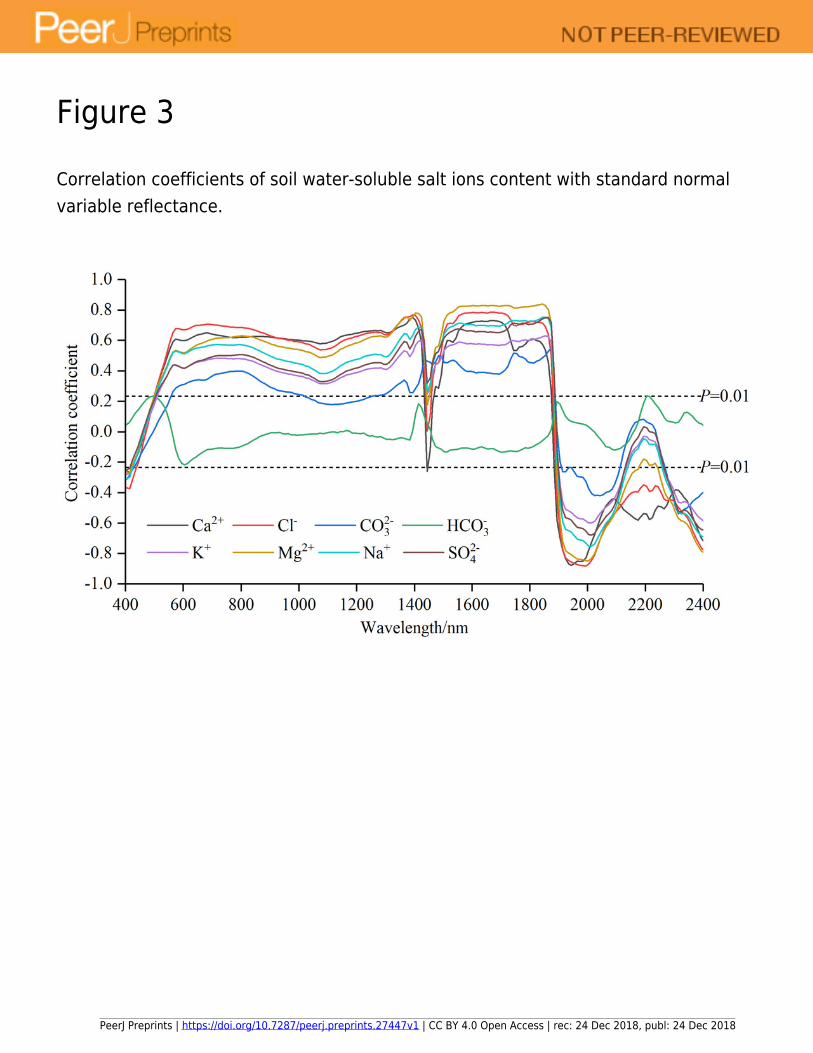
Figure 3

Correlation coefficients of soil water-soluble salt ions content with standard normal

variable reflectance.


Figure 4

Gray correlation degree (GCD) for soil water-soluble salt ions content with standard

normal variable reflectance.


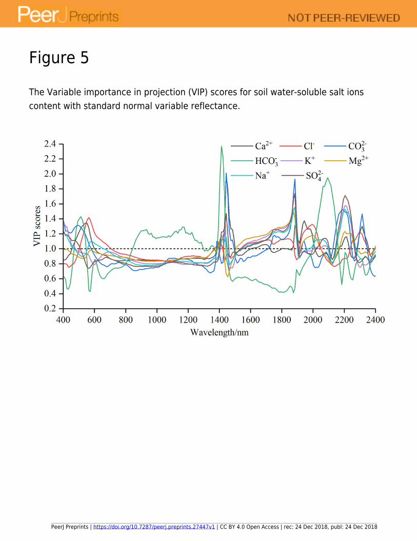
Figure 5

The Variable importance in projection (VIP) scores for soil water-soluble salt ions

content with standard normal variable reflectance.


Figure 6

Validation of soil water-soluble salt ions content based on the best model.

(A) Ca2+ with SR-SVR model. (B) Cl- with VIP-SVR model. (C) CO32- with SR-PLSR model. (D)

HCO3- with GC-PLSR model. (E) K+ with VIP-PLSR model. (F) Mg2+ with SR-SVR model. (G) Na+

with VIP-PLSR model. (H) SO42- with VIP-PLSR model.


Quantitatively estimating main soil water-soluble salt ... · 372 ions content, SR method was the...

Documents

Transcript of Quantitatively estimating main soil water-soluble salt ... · 372 ions content, SR method was the...