I

Quantitative Ultrasound Characterization and Monitoring of Locally Advanced Breast Cancer

by Hadi Tadayyon

A thesis submitted in conformity with the requirements for the degree of Doctor of Philosophy

Department of Medical Biophysics

University of Toronto

© Copyright Hadi Tadayyon 2015

II

Quantitative Ultrasound Characterization and Monitoring of Locally Advanced Breast Cancer

Hadi Tadayyon

Doctor of Philosophy

Department of Medical Biophysics

University of Toronto

2015

Abstract

Traditional assessment of tumour response to cancer therapy is based on tumour size reduction,

which takes several weeks to become clinically significant. In this thesis, novel ultrasound

backscatter signal analysis and machine learning techniques were developed to characterize breast

tumours and detect early changes correlated to response.

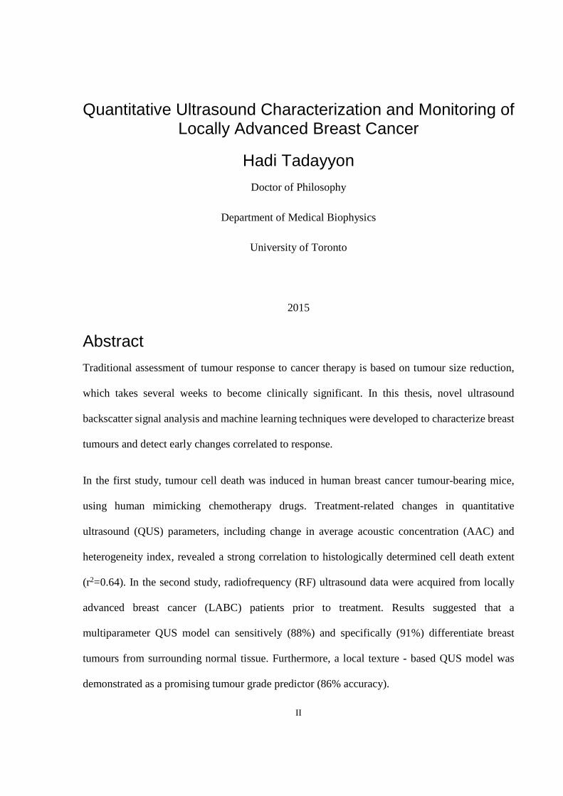
In the first study, tumour cell death was induced in human breast cancer tumour-bearing mice,

using human mimicking chemotherapy drugs. Treatment-related changes in quantitative

ultrasound (QUS) parameters, including change in average acoustic concentration (AAC) and

heterogeneity index, revealed a strong correlation to histologically determined cell death extent

(r2=0.64). In the second study, radiofrequency (RF) ultrasound data were acquired from locally

advanced breast cancer (LABC) patients prior to treatment. Results suggested that a

multiparameter QUS model can sensitively (88%) and specifically (91%) differentiate breast

tumours from surrounding normal tissue. Furthermore, a local texture - based QUS model was

demonstrated as a promising tumour grade predictor (86% accuracy).

III

In the final study, ultrasound RF data were acquired from LABC patients prior to treatment, at 3

times during the treatment (weeks 1, 4, 8), and prior to surgery. Tumour response classification

analysis using a multiparameter QUS model of midband fit (MBF), spectral slope (SS), and

spacing among scatterers (SAS) demonstrated desirable classification performance at 4 weeks into

treatment (80 ± 5%). Secondly, the QUS classification model demonstrated a significant difference

in survival rates of responding and nonresponding patients at weeks 1 and 4 (p=0.035, and 0.027,

respectively).

In summary, the incorporation of QUS assessment of the breast during or after an ultrasound-

guided breast biopsy session may potentially permit cross-verification of the histopathological

findings. Furthermore, patients undergoing neoadjuvant chemotherapy can potentially benefit

from a weekly QUS assessment in order to evaluate their early tumour response so that the

appropriate treatment intervention can be made if the patient was nonresponding.

IV

Acknowledgements

The primary acknowledgement and gratitude extends to Dr. Gregory Czarnota, who provided

valuable scientific ideas, guidance, and feedback throughout my thesis work and used enthusiastic

words such as “good work” with every progress I made. I would like to also extend my gratitude

toward my senior lab members and colleagues, Ali Sadeghi-Naini, Lakshmanan Sannachi, and

Mehrdad Gangeh, for their valuable help in data analysis methodologies and fruitful scientific

discussions. I also greatly benefited from the help of Azza Al-Mahrouki with optical microscopy,

histological data interpretation, and insightful biology discussions.

I would like to also extend a general thank-you to all members of the Czarnota lab as supportive

colleagues and friends, who made my time in the lab enjoyable. I found the scientific lab meetings

and occasional social gatherings to be a great experience. My experience with my lab mates

demonstrated that regular scientific and social discussions (during breaks) are necessary for the

morale and well-being of a researcher.

A vital component of my research success was my PhD committee, consisting of Dr. Michael

Kolios, Dr. Anne Martel, and Dr. Greg Stanisz. With their critical examination of my progress and

constructive feedback, I grew as a researcher and a critical thinker. Dr. Michael Oelze at the

University of Illinois was also a part of my PhD success, who kindly shared his laboratory’s

MATLAB program for quantitative ultrasound analysis and with whom I had fruitful discussions

about quantitative ultrasound scattering models and its application to cell death detection.

I would like to also extend my gratitude toward my family, including my father Mohammad

Tadayyon, mother, Marzieh Sari Aslani, sister, Hoda Tadayon, and wife, Narges Nooripoor for

their unconditional love and companionship in both good and hard times during my PhD journey.

This thesis was partially supported by NSERC Alexander Graham Bell Postgraduate Scholarship.

V

List of Abbreviations AAC Average acoustic concentration

AI Apoptotic Index

ACE Attenuation coefficient estimate

AR Autoregressive model

ASD Average scatterer diameter

BSC Backscatter coefficient

CDF Cell death fraction

CON Contrast texture feature

COR Correlation texture feature

dBr Decibels relative to reference

DCE-MRI Dynamic contrast enhanced MRI

DOI Diffuse Optical Imaging

DW-MRI Diffusion-weighted MRI

ENE Energy texture feature

ER Estrogen receptor

FDG Fluoro-deoxyglucose

FF Form factor (scattering model)

FFSM Fluid-filled sphere model

FFT Fast Fourier transform

GLCM Grey-level co-occurrence matrix

HER2 Human epithelial growth factor receptor 2

HI Heterogeneity index

HOM Homogeneity texture feature

ISEL In situ end labeling

KNN K nearest neighbour

LABC Locally Advanced Breast Cancer

MASD Minimum average standard deviation

MBF Midband-fit of power spectrum

MRI Magnetic Resonance Imaging

PET Position emission tomography

VI

PR Progesterone receptor

QUS Quantitative ultrasound

RECIST Response Evaluation Criteria in Solid

Tumours

ROC Receiver-operator characteristics

ROI Region of interest

RF Radiofrequency

SAC Spectral autocorrelation

SAS Spacing among scatterers

SGM Spherical Gaussian model

SI Spectral intercept (0-MHz intercept)

SS Spectral slope

TUNEL Terminal deoxynucleotidyl transferase

deoxyuridine-triphosphatase nick end labeling

VII

Contents

Abstract ........................................................................................................................................... II

Acknowledgements ....................................................................................................................... IV

List of Abbreviations ...................................................................................................................... V

List of Tables .................................................................................................................................. X

List of Figures .............................................................................................................................. XII

1 Introduction ................................................................................................................................ 1

1.1 Overview of locally advanced breast cancer management ................................................. 2

1.2 Cancer therapy response assessment and the role of ultrasound ........................................ 3

1.3 Basic principles of ultrasonic scattering in biological tissues ............................................ 5

1.4 Ultrasound radiofrequency spectrum .................................................................................. 7

1.5 Scatterer spacing estimation using spectral autocorrelation ............................................... 9

1.6 The backscatter coefficient and estimation of its parameters ........................................... 12

1.7 Frequency-dependent acoustic attenuation ....................................................................... 13

1.8 Statistical texture analysis ................................................................................................. 15

1.9 Ultrasound detection of cell death .................................................................................... 17

1.10 Quantitative ultrasound parameters investigated .............................................................. 22

1.11 Thesis overview and hypothesis ....................................................................................... 23

2 Correlation between QUS and cell death in vivo at the clinically relevant frequency range ... 26

2.1 Overview ........................................................................................................................... 27

2.2 Introduction ....................................................................................................................... 28

2.3 Methods ............................................................................................................................. 31

2.3.1 Experimental procedures ...................................................................................... 31

2.3.2 Quantitative ultrasound analysis ........................................................................... 32

2.3.3 Histology analysis ................................................................................................. 33

VIII

2.3.4 Statistical Analysis ................................................................................................ 34

2.4 Results ............................................................................................................................... 35

2.4.1 Histological assessment of treatment effects ........................................................ 35

2.4.2 Tumour volume analysis ....................................................................................... 37

2.4.3 Tissue microstructure models ............................................................................... 37

2.4.4 Ultrasonic scattering properties of cell death ........................................................ 42

2.5 Discussion and Conclusions ............................................................................................. 47

3 Quantitative ultrasound characterization of locally advanced breast cancer ........................... 51

3.1 Overview ........................................................................................................................... 52

3.2 Introduction ....................................................................................................................... 53

3.3 Methods ............................................................................................................................. 55

3.3.1 Overview ............................................................................................................... 55

3.3.2 Ultrasound data acquisition and processing .......................................................... 56

3.3.3 Quantitative ultrasound analysis ........................................................................... 59

3.3.4 Statistical textural analysis of quantitative ultrasound maps ................................ 59

3.3.5 Tissue classification algorithm ............................................................................. 60

3.4 Results ............................................................................................................................... 61

3.4.1 QUS analysis of tumour versus normal tissue ...................................................... 61

3.4.2 QUS analysis of tumour grades ............................................................................ 63

3.5 Discussion ......................................................................................................................... 69

4 Quantitative ultrasound assessment of breast tumour response to chemotherapy ................... 72

4.1 Overview ........................................................................................................................... 73

4.2 Introduction ....................................................................................................................... 74

4.3 Methods ............................................................................................................................. 76

4.3.1 Ultrasound data acquisition and processing .......................................................... 76

4.3.2 Quantitative ultrasound data analysis ................................................................... 77

IX

4.3.3 Classification and statistical analyses ................................................................... 78

4.4 Results ............................................................................................................................... 79

4.5 Discussion ......................................................................................................................... 91

5 Summary and future directions ................................................................................................ 95

5.1 Summary and conclusions of thesis .................................................................................. 96

5.2 Future directions ............................................................................................................... 98

Appendix ..................................................................................................................................... 102

Analytical solution for the scattering from solid spheres ........................................................... 103

Patient characteristics .................................................................................................................. 106

Transducer characterization and validation of scatterer size and attenuation estimation ........... 112

Overview and background ..................................................................................................... 112

Methods .................................................................................................................................. 113

Ultrasound imaging systems ........................................................................................... 113

Transducer characterization ............................................................................................ 113

Phantom construction ...................................................................................................... 114

Attenuation coefficient estimation in vivo ...................................................................... 115

Backscatter coefficient and scatterer size estimation ...................................................... 115

Results .................................................................................................................................... 116

Transducer characterization ............................................................................................ 116

Attenuation coefficient estimation in vivo ...................................................................... 117

Backscatter coefficient and scatterer size estimation in vivo .......................................... 118

Discussion .............................................................................................................................. 126

References ................................................................................................................................... 127

X

List of Tables

Table 1-1. Investigated QUS parameters, their definition, and their link to biology. .................. 22

Table 2-1. Comparison of ASDs (µm) and AACs (dBr/cm3) estimated using the SGM and FFSM

models at low and high frequencies (LF and HF) with mean histological measurement of tumour

cell size. R2 is a measure of the goodness-of-fit of the model BSCs to the measured BSCs. ±

represents standard deviations of the parameter over the tumour samples. Estimates were

obtained from all tumours prior to treatment. ............................................................................... 39

Table 2-2. Stepwise multiple regression results. The second column presents the standardized

coefficient of each model and the third column presents the model’s correlation to CDF (r2) .... 43

Table 2-3. Stepwise multiple regression results for the two cases - with and without tumour

volume normalization (separated by a horizontal line). The second column presents the

standardized coefficient of each parameter and the third column presents the parameter's

correlation to CDF (r2). NS indicates non-significant results (p>0.05). ....................................... 44

Table 3-1. Patient characteristics. ER is estrogen receptor, PR is progesterone receptor, HER2 is

the human epithelial growth factor receptor 2, IDC is invasive ductal carcinoma, and IMC is

invasive micropapillary carcinoma. Tumour size refers to the longest diameter of the tumour... 58

Table 3-2. Classifier performances using different combinations of advanced QUS parameters

for tumour versus normal tissue classification - (ASD, AAC), (ASD, SAS), (AAC, SAS) and

(ASD, AAC, SAS). AUC - area under the ROC curve. ................................................................ 63

Table 3-3. Summary of classification performances for optimal parameters obtained from

sequential feature selection from all means, all textures, and all means and textures. All results

were obtained by leave-one-out cross-validation. ........................................................................ 65

Table 3-4. Discriminant function structure vector for optimal QUS means and textures.

Coefficients represent the correlation between each parameter and the obtained discriminant

function. Parameters are listed in order of decreasing absolute coefficient. ................................ 66

Table 4-1. Summary of patient characteristics. IDC = invasive ductal carcinoma, ILC = Invasive

lobular carcinoma, BTS = bulk tumour shrinkage (percent change in tumour size). ................... 84

XI

Table 4-2. A comparison of the classification performances (accuracy) of different QUS

parameters using the KNN classifier, at weeks 1, 4 and 8. The bold entry indicates the best

performance. Reported values are mean and standard deviation of the accuracies obtained by

running the classification 10 times using 10 random samples of responders. .............................. 88

Table 4-3. A comparison of the classification results obtained based on tumour size alone

(RECIST criteria), based on changes in QUS parameters, and based on changes in QUS

parameters plus week 0 QUS parameters. ∆QUS represents [∆MBF ∆SS ∆SAS] and QUSw0

represents [MBFw0 SSw0 SASw0]. The last row presents the p-value significance of the difference

between the mean accuracies of ∆QUS and ∆QUS + QUSw0 models. Reported values are mean

and standard deviation of the accuracies obtained by running the classification 10 times using 10

bootstrap samples from responder group. For QUS results, sensitivity and specificity numbers

have denominator of 16 and accuracy numbers have denominator of 32. .................................... 88

Table 4-4. Clinical/histopathological characteristics of misclassified patients at week 4. The

majority were HER2 negative patients (indicated in bold), and the few HER2 positive patients

(indicated in italics) all received HER2 receptor-targeted treatments such as Herceptin and

Trastuzumab. ................................................................................................................................. 90

XII

List of Figures

Figure 1-1. A schematic plot of the normalized power spectrum with linear regression applied to

the – 6dB transducer bandwidth (4.5 – 9 MHz). dBr is defined as decibels relative to reference.

Adapted from [36]. .......................................................................................................................... 8

Figure 1-2. (A) Typical power spectrum estimated using the AR model from a human breast

tumour. (B) Corresponding spectral autocorrelation functions for different AR model order (p =

10-100). At lower orders (p < 50), no peaks can be detected. At p = 100, false peaks appear. .... 11

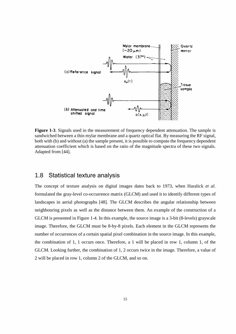
Figure 1-3. Signals used in the measurement of frequency dependent attenuation. The sample is

sandwiched between a thin mylar membrane and a quartz optical flat. By measuring the RF

signal, both with (b) and without (a) the sample present, it is possible to compute the frequency

dependent attenuation coefficient which is based on the ratio of the magnitude spectra of these

two signals. Adapted from [42]. ................................................................................................... 15

Figure 1-4. Process of GLCM computation. The left matrix is an 3-bit grayscale image and the

right matrix is the corresponding GLCM constructed using a distance of one pixel and an angle

of 00. Adapted from [47]. .............................................................................................................. 16

Figure 1-5. Integrated backscatter coefficient versus nuclear diameter of a cell. The data were

acquired from whole cells, with the diameter of the cell nucleus plotted along the x-axis. The

square denotes the MT-1 cell line for which the nuclear diameter was measured by visual

inspection of the microscopy images of whole cells. Adapted from [43]. ................................... 19

Figure 1-6. Results of photodynamic therapy on in vivo xenograft tumours. Tumours were

examined using 26-MHz ultrasound before treatment and at different times after administration

of PDT (n = 3 animals per time). Ultrasound data collection consisted of acquiring B-scan

images (A) in addition to spectroscopic data for quantitative analyses of backscattered ultrasound

(B,C). At 24 h, there was an increase in backscatter that was detected in ultrasound images, as

well as in spectroscopic data. (D) TUNEL sections at 40× magnification. Typical changes of

apoptosis were observed, including nuclear coalescence and fragmentation, as the function of

time. At 48 h, nearly half of the cells in the treated area had lost their nuclei as in a final stage of

XIII

apoptotic cell death. These changes explain the detected changes in variables related to the size

of scatterers in the tissue by ultrasound. Adapted from [25]. ....................................................... 21

Figure 1-7. Scattering simulation with pseudo-regular spacing of cells. Left: a typical pseudo-

regular cell array with random loss of nuclei. This array was used as input data for the

simulation. Predictions of the average signal amplitude if, in a random way throughout the cell, a

fraction of the nuclei, or its fragments, have disappeared during apoptosis. Adapted from [49]. 21

Figure 2-1. (A-D) Histology images of representative control, 4-hour, 12-hour, 24-hour, and 48-

hour chemotherapy-treated MDA-231 tumours, from left to right, respectively. (A) Low-

magnification H&E stained sections. (B) Low-magnification ISEL stained sections (C) High-

magnification H& E stained section to highlight nuclear material. (D) High-magnification ISEL

section to highlight fragmented DNA. The control tumour features rapidly dividing cells with

large nuclei. The treated tumours feature reduced nuclear size (nuclear condensation),

fragmented nuclei, and dead cellular components filling the extracellular space (brown stains).

The low-magnification scale bar represents 1 mm. The high-magnification scale bar represents

25 µm. (E) Plots of mean cell and nucleus diameters versus treatment time (0 to 48 hours),

estimated from H& E histology sections. Error bars represent standard error of the mean. (F) Plot

of the mean cell death fractions versus time. Error bars represent the standard error across the

tumour samples for each time condition. Statistical significance: * = p<0.05. ............................ 36

Figure 2-2. Plot of in vivo tumour volumes before (pre) and at predefined length of time after

chemotherapy injection (post). Percent errors of the initial tumour volumes for each group were

74%, 27%, 40%, 20%, and 67%, for control, 4-hour, 12-hour, 24-hour, and 48-hour groups,

respectively. .................................................................................................................................. 37

Figure 2-3. Illustration of the spatial distribution of R2 goodness of fits of the SGM and FFSM

models over different tumour areas. Presented are R2 images overlaid on analyzed tumour ROIs

over three tumour cross-sections: upper limb, tumour center, and lower limb. Data is presented

from the low-frequency study with (A) 2 × 2 mm RF windows and (B) 3 × 3 mm RF windows.41

Figure 2-4. Combined low and high frequency plots of measured BSC and theoretical BSCs

based on the SGM and FFSM models obtained from an animal in the 24-hour treatment group.

XIV

Left: pre-treatment. Right: post-treatment. The BSCs were obtained from an RF window at the

center of the tumour ROI. Corresponding R2 goodness of fit values are shown below the plots. 42

Figure 2-5. Pre- and post- treatment (24h) images of the central cross section of a sample MDA-

231 tumour which received chemotherapy treatment. (A) and (B) show ASD and AAC images

overlaid on the B-mode image obtained from the high-frequency and low frequency systems,

respectively, and (C) shows low and high magnification ISEL-stained histology sections of the

tumour post treatment. B-mode scale bar represents 2 mm. Low magnification represents 1mm.

High magnification represents 25µm. ........................................................................................... 45

Figure 2-6. Results of QUS analysis of cell death. (A) Plot of ∆AAC versus time from treatment

onset obtained using the low and high frequency systems. Error bars represent the standard error

across the tumour samples for each time condition. Statistical significance: * = p<0.05. (B)

Scatter plot of CDF versus the predictive model (∆AAC, ∆HIASD), r2=0.639. (C) Scatter plot of

CDF versus the predictive model (∆AAC, ∆HIASD, and Vi ), r2 = 0.744. ..................................... 47

Figure 3-1. 2-D scatter plot of SAS versus AAC of tumours and normal tissues. The class

dividing curve represents the quadratic discriminant function. .................................................... 62

Figure 3-2. Receiver operator characteristics curves for the different parameter sets. Set A:

means and textures of MBF, SS, SI, and SAS, plus ACE. Set B: means and textures of ASD,

AAC, and SAS, plus ACE. Set C, all parameter means and textures included. ........................... 67

Figure 3-3. One-dimensional scatter plot of the hybrid QUS Biomarker versus tumour

aggressiveness. Each point represents the hybrid QUS value of each patient. The horizontal lines

represent the means of the groups. ................................................................................................ 67

Figure 3-4. Representative images of grade I, II, and III breast tumours. (A) B-mode images of

the tumour regions, where the tumours appear as hypoechoic masses. (B) Corresponding hybrid

QUS biomarker images of the tumours obtained from optimized linear combination of original

QUS means and textures. A common scale bar was used to include the range for all three

tumours (C) Same images as (B) but with the use of individual scale bars to show the tumour

heterogeneity (D) Hematoxylin and eosin stained histopathology images of the tumours. Scale

bars: 1 cm (US), 100 µm (hist). .................................................................................................... 68

XV

Figure 4-1. Representative B-mode images (A), MBF images (B), power spectra (C left) before

and 4 weeks after the start of chemotherapy treatment and hematoxylin and eosin histology

histology images (C right) of an example responding breast tumour. Data in the left column

represent pre-treatment data, obtained prior to treatment initiation, and data in the right column

represent week 4 data. US scale bar represents 1 cm, histology scale bar represents 100 µm. .... 85

Figure 4-2. Representative B-mode images (A), MBF images (B), power spectra (C left) before

and 4 weeks after the start of chemotherapy treatment and hematoxylin and eosin histology

histology images (C right) of an example nonresponding breast tumour. Data in the left column

represent pre-treatment data, obtained prior to treatment initiation, and data in the right column

represent week 4 data. US scale bar represents 1 cm, histology scale bar represents 100 µm. .... 86

Figure 4-3. Comparison between QUS parameters (A-G) and the RECIST-based tumour size

reduction (H) for tracking patient tumours during chemotherapy. QUS and RECIST values were

averaged over responder (blue diamond) and non-responder (red square) groups, and plotted over

the treatment time. Patients were grouped based on their pathological clinical response

determined post-chemotherapy. All values were normalized to week 0 by subtraction. Error bars

represent standard error of the mean. ............................................................................................ 88

Figure 4-4. Kaplan-Meier survival curves for responding (solid line) and nonresponding (dashed

line) patients. (A) Patients were classified based on clinical/histopathological information.

(B,C,D) Patients were classified based on the QUS biomarkers (including week 0 data) obtained

at weeks 1, 4, and 8, respectively. ................................................................................................. 89

Figure 5-1. Softvue Ultrasound computed tomography system. The system comprises of over

2000 transducer elements arranged in a ring which operate both in transmission and reflections

modes. Adapted from Delphinus Medical Technologies (http://www.delphinusmt.com/our-

technology/softvue-system) ........................................................................................................ 101

Figure 5-2. Using a patented 360 degree rotating concave ultrasound transducer, SonixEmbrace

Research captures realistic, uncompressed images of a breast, while the patient lies in a

comfortable, prone position. The system captures gigabytes of raw data, which is ideal for cancer

detection research and treatment monitoring. Adapted from Analogic Ultrasound

(http://www.analogicultrasound.com/research/clinical/applications/breast-cancer) .................. 101

1

1 Introduction

2

1.1 Overview of locally advanced breast cancer management

Breast cancer continues to be the predominant form of cancer affecting Canadian women over the

age of 20. In 2013, 23, 800 Canadian women were diagnosed with breast cancer, and an estimated

5000 women died [1]. Locally advanced breast cancer (LABC) is a relatively aggressive subtype

of breast cancer that includes stage 3 tumours (T3N0 and T3N1) 5 cm or larger often with

involvement of the axillary lymph nodes, skin, and/or chest wall. Despite management efforts

using systemic therapy, surgery, and radiotherapy, the prognosis of LABC patients is relatively

poor with five-year survival rates below 50% [2]. Women at high risk of having or developing

breast cancer are screened with combined mammography and ultrasound [3], and based on the

findings, a breast biopsy may be recommended to the patient in order to obtain a definitive

diagnosis. As clinical studies have shown, the preferred modality for staging LABC, in addition to

biopsy, is magnetic resonance imaging (MRI), owing to its superior ability to visualize extent of

disease, multicentricity, and mammographically occult cancers [4]. However, ultrasound is

emerging as an adjunct modality for locoregional staging of LABC diseases due its good spatial

resolution, cost effectiveness, and availability [5].

LABC is generally inoperable and requires upfront chemotherapy treatment for local and

metastatic control and to facilitate breast conserving surgery. LABC is a heterogeneous disease

encompassing a wide range from low-grade ER/PR/HER2 positive breast cancers to high-grade

ER/PR/HER2 negative breast cancers. The typical management workflow for these patients is

neoadjuvant chemotherapy, followed by surgery (lumpectomy or mastectomy), and then by

radiation therapy. Chemotherapy is often administered using a combination of taxanes,

anthracyclines, fluorouracil, and cyclophosphamide. Taxane drugs are plant-derived drugs that act

as microtubule disrupters, thereby inhibiting the process of cell division. Anthracyclines are a

bacteria-derived class of drugs that inhibit DNA and RNA synthesis in cells, by intercalating the

base pairs of the DNA/RNA strands. Chemotherapy administration is typically fractionated (into

cycles) in order to help patients recover from drug effects. The administration schedule is typically

once every 2 or 3 weeks and the duration varies from 18 to 24 weeks.

Patients with similar tumour types often respond differently to the same chemotherapy drug; thus,

switching to a more aggressive drug as a result of poor response to treatment is not uncommon in

LABC patients. Conventional methods of clinical tumour response assessment involve tracking

3

changes in tumour size (longest diameter) using the guidelines provided by Response Evaluation

Criteria in Solid Tumours (RECIST) [6]. This can be achieved by intratreatment measurements of

tumour dimensions by clinical examination, X-ray mammography, MRI, and/or conventional

ultrasound imaging. However, bulk mass diminishments do not typically occur until several weeks

to a few months after treatment initiation, despite cytotoxic effects induced by the treatment [7].

Thus, the introduction of an imaging modality capable of differentiating between responding and

nonresponding patients in the first days/weeks of a lengthy treatment regimen, would allow

clinicians to rapidly determine the effectiveness of a cancer drug, resulting in improved patient

prognosis.

1.2 Cancer therapy response assessment and the role of ultrasound

The currently accepted method of response assessment is based on a reduction in the sum of the

largest diameters of target lesions or the largest diameter of unifocal disease [6]. However,

clinically detectable tumour shrinkage does not typically occur until several weeks to months into

treatment. Consequently, imaging assessments of tumour biology and biochemistry have led to the

discovery of novel biomarkers that can provide earlier indications of tumour response to therapy

[7]. Research in early detection of breast cancer response to anticancer therapy has led to

discoveries in both image-based and chemical-based biomarkers. In a prospective clinical study,

Chang et al. monitored levels of apoptotic index (AI) and Ki-67 in breast cancer patients

undergoing chemotherapy through flow cytometric and immunocytochemical analyses of fine

needle aspiration samples obtained from the breast tumours [8]. Whereas AI represents the number

fraction of apoptotic cells identified through terminal deoxynucleotidyl transferase deoxyuridine-

triphosphatase nick end labeling (TUNEL), staining for DNA fragmentation, Ki-67 represents

cancer cell proliferation. In that study, an increase in AI after 1-3 days, and a decrease in Ki-67

after 21 days, all significant, were found in responding patients compared to nonresponding ones.

In another study by Nishimura et al. [9], a higher Ki-67 index was found to be associated with

poorer disease-free survival of breast cancer patients.

As for image-based markers, diffusion-weighted MRI (DW-MRI) has been demonstrated

clinically to predict response of breast tumours as early as after 1 cycle of chemotherapy. It is used

4

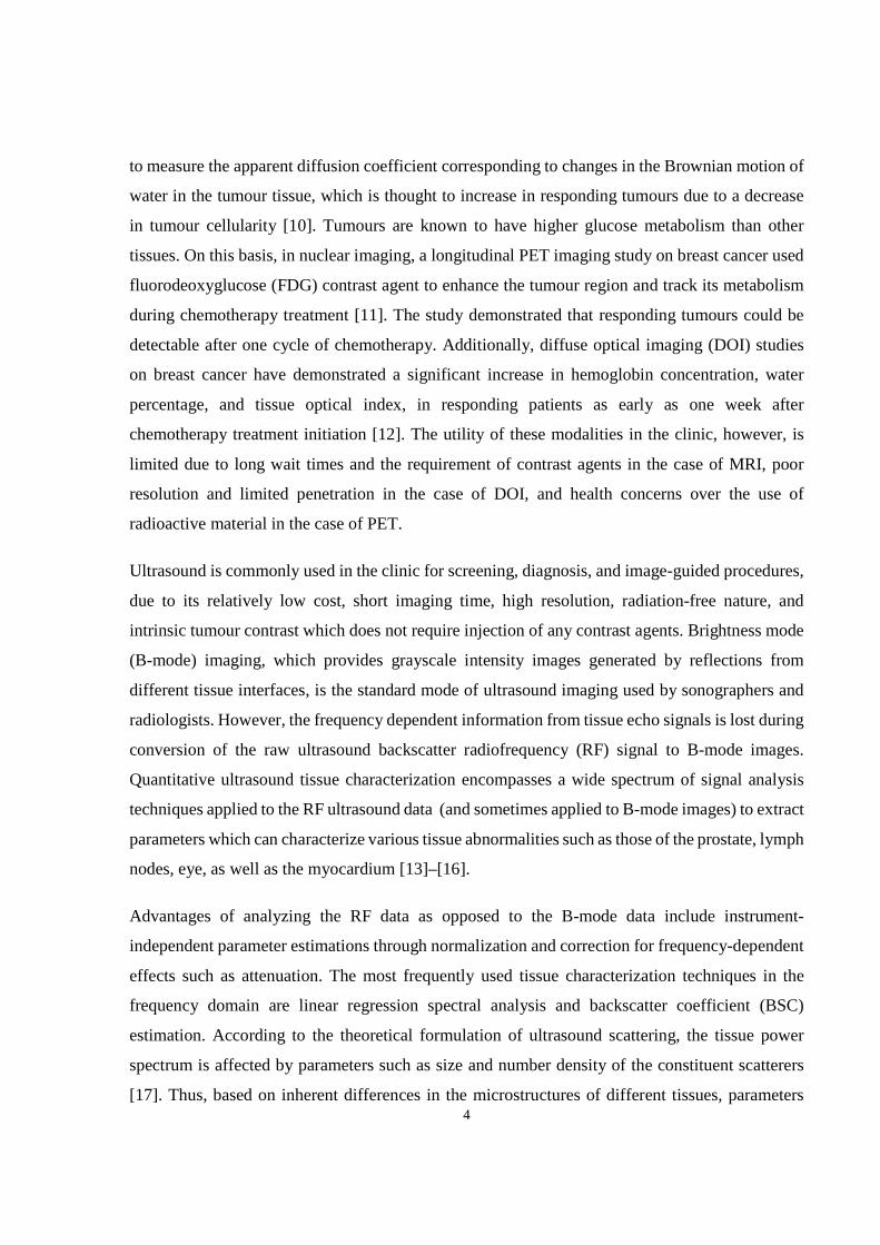
to measure the apparent diffusion coefficient corresponding to changes in the Brownian motion of

water in the tumour tissue, which is thought to increase in responding tumours due to a decrease

in tumour cellularity [10]. Tumours are known to have higher glucose metabolism than other

tissues. On this basis, in nuclear imaging, a longitudinal PET imaging study on breast cancer used

fluorodeoxyglucose (FDG) contrast agent to enhance the tumour region and track its metabolism

during chemotherapy treatment [11]. The study demonstrated that responding tumours could be

detectable after one cycle of chemotherapy. Additionally, diffuse optical imaging (DOI) studies

on breast cancer have demonstrated a significant increase in hemoglobin concentration, water

percentage, and tissue optical index, in responding patients as early as one week after

chemotherapy treatment initiation [12]. The utility of these modalities in the clinic, however, is

limited due to long wait times and the requirement of contrast agents in the case of MRI, poor

resolution and limited penetration in the case of DOI, and health concerns over the use of

radioactive material in the case of PET.

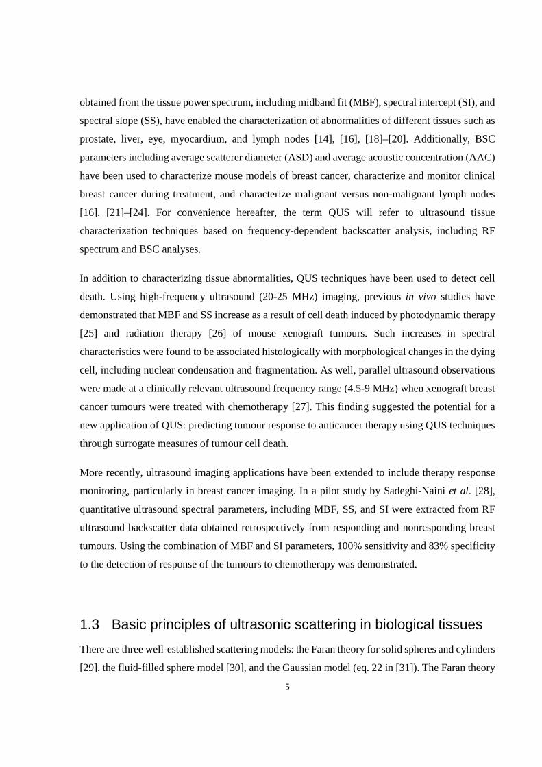
Ultrasound is commonly used in the clinic for screening, diagnosis, and image-guided procedures,

due to its relatively low cost, short imaging time, high resolution, radiation-free nature, and

intrinsic tumour contrast which does not require injection of any contrast agents. Brightness mode

(B-mode) imaging, which provides grayscale intensity images generated by reflections from

different tissue interfaces, is the standard mode of ultrasound imaging used by sonographers and

radiologists. However, the frequency dependent information from tissue echo signals is lost during

conversion of the raw ultrasound backscatter radiofrequency (RF) signal to B-mode images.

Quantitative ultrasound tissue characterization encompasses a wide spectrum of signal analysis

techniques applied to the RF ultrasound data (and sometimes applied to B-mode images) to extract

parameters which can characterize various tissue abnormalities such as those of the prostate, lymph

nodes, eye, as well as the myocardium [13]–[16].

Advantages of analyzing the RF data as opposed to the B-mode data include instrument-

independent parameter estimations through normalization and correction for frequency-dependent

effects such as attenuation. The most frequently used tissue characterization techniques in the

frequency domain are linear regression spectral analysis and backscatter coefficient (BSC)

estimation. According to the theoretical formulation of ultrasound scattering, the tissue power

spectrum is affected by parameters such as size and number density of the constituent scatterers

[17]. Thus, based on inherent differences in the microstructures of different tissues, parameters

5

obtained from the tissue power spectrum, including midband fit (MBF), spectral intercept (SI), and

spectral slope (SS), have enabled the characterization of abnormalities of different tissues such as

prostate, liver, eye, myocardium, and lymph nodes [14], [16], [18]–[20]. Additionally, BSC

parameters including average scatterer diameter (ASD) and average acoustic concentration (AAC)

have been used to characterize mouse models of breast cancer, characterize and monitor clinical

breast cancer during treatment, and characterize malignant versus non-malignant lymph nodes

[16], [21]–[24]. For convenience hereafter, the term QUS will refer to ultrasound tissue

characterization techniques based on frequency-dependent backscatter analysis, including RF

spectrum and BSC analyses.

In addition to characterizing tissue abnormalities, QUS techniques have been used to detect cell

death. Using high-frequency ultrasound (20-25 MHz) imaging, previous in vivo studies have

demonstrated that MBF and SS increase as a result of cell death induced by photodynamic therapy

[25] and radiation therapy [26] of mouse xenograft tumours. Such increases in spectral

characteristics were found to be associated histologically with morphological changes in the dying

cell, including nuclear condensation and fragmentation. As well, parallel ultrasound observations

were made at a clinically relevant ultrasound frequency range (4.5-9 MHz) when xenograft breast

cancer tumours were treated with chemotherapy [27]. This finding suggested the potential for a

new application of QUS: predicting tumour response to anticancer therapy using QUS techniques

through surrogate measures of tumour cell death.

More recently, ultrasound imaging applications have been extended to include therapy response

monitoring, particularly in breast cancer imaging. In a pilot study by Sadeghi-Naini et al. [28],

quantitative ultrasound spectral parameters, including MBF, SS, and SI were extracted from RF

ultrasound backscatter data obtained retrospectively from responding and nonresponding breast

tumours. Using the combination of MBF and SI parameters, 100% sensitivity and 83% specificity

to the detection of response of the tumours to chemotherapy was demonstrated.

1.3 Basic principles of ultrasonic scattering in biological tissues

There are three well-established scattering models: the Faran theory for solid spheres and cylinders

[29], the fluid-filled sphere model [30], and the Gaussian model (eq. 22 in [31]). The Faran theory

6

is the most accurate model when the exact scatterer geometry is known, and thus commonly used

for characterizing tissue-mimicking ultrasound phantoms which contain glass beads [32]. This

theory gives the closed form solution of the scattered pressure by a solid sphere (or cylinder) when

irradiated by an incident plane wave. The caveat of Faran's theory is the analytical complexity.

Because of this, analytically simpler models have been developed by assuming weak scattering

(ignoring multiple scattering) and ignoring shear wave propagation. These models are called form

factor models. A form factor is a measure of frequency-dependent scattering based on the shape,

size and mechanical properties of the constituent scatterers. Particularly, the Gaussian form factor

(FF), expressed by equation 0, has been used frequently to model scattering by soft tissues [14–

16] as it represents a distribution of gradually changing acoustic impedance between the scatterer

and the background material. The fluid-filled sphere form factor (equation 1.2) represents

scattering from a fluid-filled scatterer in a fluid-like medium. The models are expressed as follows

[31]:

�������2� = �� .������� 1.1.

�����2� = ����2��23 �� �� 1.2.

In the above formulas, �� is the spherical Bessel function of the first kind and first order, � = ����

is the wavenumber, is sound speed, ! is frequency, and � is scatterer radius. The parameter

usually measured for estimating scatterer properties is the BSC. The BSC is a frequency-dependent

function that represents the backscattered power per unit solid angle normalized to incident

intensity [33]. Result validations often involve comparison of the measured BSC to a theoretical

model, which incorporates the form factor (FF). A BSC can be related to a form factor,���, �, by the following relation [34],

#$�� = %&9 �(�)*����, � 1.3.

where n&γ� is the average acoustic concentration, AAC, k = �./0 is the wave number, a is the

scatterer radius, and γ� is the mean square deviation between the impedance of the scatterers and

the surrounding medium. In this equation, impedance is the product of density (ρ) and speed (c).

7

1.4 Ultrasound radiofrequency spectrum

As previously mentioned, analysis of the frequency content of the backscattered tissue signal

permits characterization of the tissue in terms of its microstructure. By modeling the tissue echo

power spectrum (ultrasound radiofrequency spectrum) as a linear approximation of the Fourier

transform of the acoustic impedance autocorrelation, Lizzi et al. demonstrated that SS is related to

the scatterer size and SI and MBF can be related to the scatterer concentration [17]. These

parameters are estimated from a linear regression analysis of the tissue power spectrum within the

usable bandwidth (usually corresponding to −6 dB range). An ultrasound RF image region of

interest (ROI) usually consists of smaller blocks (windows) in which the power spectra are

calculated. Figure 1-1 presents a schematic plot of the normalized power spectrum in an RF

window, corresponding linear regression line, and a graphical description of the spectral

parameters. The amplitude line spectrum, 23�!, 43, of a gated RF line segment, 43, can be

calculated using the reference phantom technique [35], as shown in equation 1.4. In this equation, 2��!, 43 is the fast Fourier transform (FFT) of an RF line segment of the sample after gating with

a Hanning window, and 25�!, 43 is the FFT of the gated RF signal from a calibration reference.

The log power spectrum, 6�!, can then be computed by averaging the squared magnitudes of the

amplitude line spectra laterally across the window, compensating for sample and reference

attenuation, and taking the log of the result, as presented in equation 1.5 [35]. The attenuation

coefficients of the sample and reference are7� and 75, respectively; R is the range (transducer to

proximal edge of window); and ∆4 is the window length (axial).

23�!, 43 = 2��!, 4325�!, 43 1.4.

6�! = log� 1=>|23�!, 43|���(�@A�@B�CD∆E� F3G� 1.5.

8

While 25�!, 43 can refer to the spectrum of a planar reflector or a phantom, in this thesis, a

phantom is used as the reference for RF spectral analysis in order to facilitate depth-dependent

corrections.

A line of best fit, using least squares, can be found for the normalized power spectrum within the

-6 dB frequency bandwidth as per Lizzi’s method [17], 6�! = 66! + 6I 1.6. JK� = 6�!� 1.7.

where 66 and 6I are the slope and extrapolated 0-MHz intercept of the line of best fit, and JK�

is the solution of the line-approximated power spectrum at the center of the frequency bandwidth

(i.e., 6.75 MHz in the example plot). The bandwidth was determined from the power spectrum of

a reference phantom.

Figure 1-1. A schematic plot of the normalized power spectrum with linear regression applied to the – 6dB transducer bandwidth (4.5 – 9 MHz). dBr is defined as decibels relative to reference. Adapted from [36].

9

1.5 Scatterer spacing estimation using spectral autocorrelation Scatterer spacing, also known as spacing among scatterers (SAS), is defined as the distance

between regularly spaced or periodic scatterers in a medium. It is computed from the

autocorrelation of the power spectrum estimated by the autoregressive (AR) model. This method

has been demonstrated to detect distance between periodic scatterers in tissue microstructures

having lower orders of regularity [37], such as those of the liver, for characterization of liver

diseases [38]–[40]. The AR model predicts the output of a stationary stochastic process as a linear

combination of previous samples of its output, and is defined as [41],

�̂�[N] = >���̂�[N − �]Q�G� +R[N], 1.8.

where �� , � = 1, . . , Sare the AR coefficients, R[N] is a white noise input sequence, and S is the

order of the AR model. The power spectrum,|T(!)|�, can be obtained by Fourier transforming

both sides of equation 1.8 to yield [42],

|T(!)|� = U�|1 + ∑ ����W����|Q�G� �, 1.9.

where U is the standard deviation of the white noise. As demonstrated in equation 1.10, the

normalized power spectrum,6(!), can be obtained in a manner similar to that shown in the

previous section, except that the numerator was an AR-estimated power spectrum (|T(!)|�) and

the denominator was echo data from a polished Plexiglas surface, �5(NX). The subscript “n”

represents discrete depth intervals% = 1,2, … , 6 [. Also �5(NX) was independent of lateral

location,\], as the power spectra of the reflector echoes were averaged across the RF lines over

the image width to obtain a smooth mean power spectrum. This was done to obtain a good signal-

to-noise ratio and to average out any microscopic variances in the planar reflector's surface.

6(!, \]) = ∑ |T(!, \])]̂GF |�∑ |��_(�5(NX))|�]̀G , % = 1,2, . . , 6 [. 1.10.

10

Finally, the autocorrelation of the normalized AR power spectrum, a��(∆!), was computed using

equation 1.11,

a��(∆!) = > 6(!)6(! − ∆!),F

∆�G� 1.11.

which is termed the spectral autocorrelation (SAC). The SAS corresponds to the frequency

lag,∆!Q, at which the first peak in the SAC occurs,

626 = 2∆!Q, 1.12.

where is the mean speed of sound in the tissue of interest. For normal tissue ROIs, which

encompassed mainly glandular tissue, a speed of sound of 1455 m/s is assumed while for tumour

ROIs, a speed of sound of 1540 m/s is assumed. These values are consistent with tomography

measurements of the speed of sound in the breast [43].

Figure 1-2A presents an example AR-estimated power spectrum from a human breast tumour ROI,

and Figure 1-2B presents the corresponding SAC plots computed using different model order (S)

values, varying from S = 10to100. The arrows indicate the location of the first peak, from which

SAS is computed. It can be observed that at lower S values, the SAC peaks are difficult or

impossible to discern due to the low power spectrum resolution. As S increases, and therefore the

number of AR coefficients increases, the peak becomes more discernable. However, if S becomes

too large, i.e. 100 or larger, multiple peaks start to appear, resulting in false peak detection. In this

thesis, S = 50 was found to be the optimal balance between power spectrum resolution and false

peak detection and was selected for all SAC and SAS computations in the breast tissue.

11

A

B

Figure 1-2. (A) Typical power spectrum estimated using the AR model from a human breast tumour. (B) Corresponding spectral autocorrelation functions for different AR model order (p = 10-100). At lower orders (p < 50), no peaks can be detected. At p = 100, false peaks appear.

12

1.6 The backscatter coefficient and estimation of its parameters

Scatterer property estimation (i.e., scatterer size and acoustic concentration) in tissue

characterization involves finding an optimal match between a theoretical model and the

experimentally derived values of the BSC curve by varying the parameters of the model. The

theoretical formulation was already defined in equation 1.3. Next the BSC must be determined

experimentally (#e$) from the obtained RF data. #e$ can be computed from the normalized power

spectrum at the focus, 6�(!), after applying a scaling factor consisting of transducer aperture area

(2 )and target distance (a�), as presented in equation 1.13 [34]. Note that 6�(!) is the planar

reflector normalized power spectrum obtained by placing the transducer's focus in the centre of

the sample. Whereas the aperture area of a single-element focused transducer can be simply

calculated as fg�(r = radius of the aperture), an array transducer has a synthetic aperture which

requires knowledge of the range-dependent aperture opening function to compute its area. This

function defines the number of receive elements as a function of depth (axial distance from the

transducer surface). With this knowledge, one can obtain the aperture area at focal depth. This

method of BSC estimation requires prior repeated measurements of planar reflector echo at all

depths for which the sample windows are located. Alternatively, a reference phantom can be used

to estimate the BSC of a sample given the known BSC of the phantom, #$5(!), and the phantom-

normalized power spectrum,6(!), using equation 1.14 [35].

#$5(!) = 1.45a�2 6�(!), 1.13.

#e$(!) = 6(!)#$5(!)�((@A�@B)(CD∆E� ) 1.14.

Once the #e$(!) corresponding to an ROI in the sample has been obtained, the ASD from the ROI

can be estimated by minimization of the average standard deviation (MASD) between the

estimated and theoretical BSCs as follows (ref [31], equation 43):

J26i = [j% k1[>T] − T&)l

]G�m 1.15.

T] = log( #$n(!])#$(�, !])) 1.16.

13

T& = 1=>T]F

]G� 1.17.

where !] , j = 1,… ,[ is the frequency vector for which FFT data have been computed within the -

6 dB system bandwidth. Finally, ASD is derived as the average scatterer diameter (2�) of the

theoretical BSC, #$(�, !]),corresponding to the MASD. Once the ASD has been obtained by

model fitting, one can estimate the AAC (%&*�) by substituting #e$ for #$ in equation 1.3 and

solving for %&*�. In order to validate the estimation of ASD using this fitting algorithm, I applied

this algorithm on an ultrasound phantom consisting of glass microspheres embedded in agar gel.

The glass microspheres served as the scatterers with a known size distribution. I used Faran’s

theory of sound scattering from solid spheres [29] to predict the scattering from the phantom and

performed fitting between this function and the measured BSC (obtained using our linear array

transducer) to estimate the ASD. Details of the methods and results are provided in the Appendix

under “Transducer characterization and validation of scatterer size and attenuation estimation”.

Details about Faran’s theory can be found in the Appendix under “Analytical solution for scattering

from solid spheres”.

1.7 Frequency-dependent acoustic attenuation

The power spectrum and BSC measurements are affected by the inherent frequency-dependent

attenuation of intervening tissues, and, if not corrected, will yield inaccurate estimates of scattering

properties. Frequency-dependent attenuation has been shown to be a useful parameter in

characterizing tissues, especially tumours and normal tissues of the breast [44]. Additionally, a

previous clinical study found large variations in the attenuation coefficient values among breast

tumours (1.16 ± 0.8dB/cm/MHz) [22]. Attenuation loss from homogeneous samples can be

estimated by an insertion-loss method [44]. Figure 1-3 illustrates the insertion-loss technique. In

this method, an ultrasonic pulse is transmitted from the transducer toward a planar reflector which

is coupled with degassed water. The power spectrum of the transmitted pulse, 6o(!), is computed

from the RF echo of the reflector. Then, the attenuating sample is placed between the transducer

and the reflector to evaluate the change in the reflected power spectrum (6p(!)) as a result of

14

adding the sample. The attenuation coefficient (7) is found from the log difference of attenuated

(2q(!)) and un-attenuated (2r(!)) amplitude spectra, written as [45],

7(!) = 75(!) + 202s tuv w2r(!)2q(!)x 1.18.

where 75 is the attenuation function of the reference medium (typically PBS or degassed water) s

is the thickness of the attenuating sample in the longitudinal sound propagation direction, and the

factor of 2 accounts for the round trip of the ultrasound wave. For breast tissues, the power law

relationships lie in the range of n = 0.8 to 1.9 [44]. Whereas for a homogeneous sample the

attenuation coefficient holds throughout the sample, equation 1.18 does not apply to the local

attenuation coefficient of a heterogeneous sample. A more rigorous method is required to estimate

the local attenuation coefficients in a homogeneous region of a heterogeneous sample. To achieve

this, Labyed et al. developed the reference phantom algorithm, a method of estimating the local

attenuation coefficient of a locally homogeneous region in an ultrasound image by estimating the

rate of change in the spectral magnitude with depth and frequency relative to a reference medium

with a known attenuation coefficient [46]. I validated this method of attenuation coefficient

estimation using a reference phantom. Details of the validation work is provided in the Appendix

under “Transducer characterization and validation of scatterer size and attenuation estimation.”

Once the attenuation for the sample of interest has been found, the power spectra calculations can

be corrected for attenuation by multiplying by the term [47],

2(!) = �(@�yz 1.19.

where % is the exponent of the frequency power law, varying depending on the tissue. The

correction term must be for used for every attenuating layer the ultrasound passes through,

including water (although the attenuation of water is negligible at low frequencies).

15

Figure 1-3. Signals used in the measurement of frequency dependent attenuation. The sample is sandwiched between a thin mylar membrane and a quartz optical flat. By measuring the RF signal, both with (b) and without (a) the sample present, it is possible to compute the frequency dependent attenuation coefficient which is based on the ratio of the magnitude spectra of these two signals. Adapted from [44].

1.8 Statistical texture analysis

The concept of texture analysis on digital images dates back to 1973, when Haralick et al.

formulated the gray-level co-occurrence matrix (GLCM) and used it to identify different types of

landscapes in aerial photographs [48]. The GLCM describes the angular relationship between

neighbouring pixels as well as the distance between them. An example of the construction of a

GLCM is presented in Figure 1-4. In this example, the source image is a 3-bit (8-levels) grayscale

image. Therefore, the GLCM must be 8-by-8 pixels. Each element in the GLCM represents the

number of occurrences of a certain spatial pixel combination in the source image. In this example,

the combination of 1, 1 occurs once. Therefore, a 1 will be placed in row 1, column 1, of the

GLCM. Looking further, the combination of 1, 2 occurs twice in the image. Therefore, a value of

2 will be placed in row 1, column 2 of the GLCM, and so on.

16

Figure 1-4. Process of GLCM computation. The left matrix is an 3-bit grayscale image and the right matrix is the corresponding GLCM constructed using a distance of one pixel and an angle of 00. Adapted from [49].

Based on the statistical information provided by a GLCM, 14 textural features can be obtained.

For this thesis, four of these features were used, those most relevant to tissue characterization:

contrast, correlation, homogeneity, and energy. These are defined below.

{|= = > (j − })� >>S(j, }F~

WG�

F~

]G�

F~��

]�WG

1.20.

�=� >>S�j, }�F~

WG�

F~

]G�

1.21.

�|J >> S�j, }1 H |j P }|

F~

WG�

F~

]G�

1.22.

{|a ∑ ∑ �j P �]�} P �W�S�j, }F~

WG�F~]G�

#]#W 1.23.

where S�j, } is an element in a =� � =� GLCM, where =� is the number of gray levels, �] , #] are

the mean and standard deviation of the i'th row of the GLCM, and �W , #W are the mean and standard

17

deviation of the j'th column of the GLCM. The contrast parameter represents a measure of

difference between the lowest and highest intensities in a set of pixels. The energy parameter

measures the frequency of occurrence of pixel pairs and quantifies its power (square of the

frequency of gray-level transitions). The homogeneity parameter measures the incidence of pixel

pairs of different intensities. As the frequency of pixel pairs with close intensities increases,

homogeneity increases. The correlation parameter measures the intensity correlation between pixel

pairs.

1.9 Ultrasound detection of cell death

In addition to characterizing tissue abnormalities, QUS techniques have been used to detect cell

death. In an initial study using high frequency (40 MHz) ultrasound, where acute myeloid leukemia

cells were treated with cisplatinum (a chemotherapeutic agent), a 25-to-50 fold increase in the US

backscatter intensity was observed in apoptotic cells compared to viable cells. This observation

led to the hypothesis that the cell nucleus is the source of ultrasound scattering, and that it is the

morphological changes occurring in the nucleus during apoptosis that causes such ultrasound

backscatter changes. This hypothesis was investigated by Taggart et al. [45], where they

demonstrated experimentally that cells with larger nuclear diameters express higher integrated

backscatter coefficients (Figure 1-5). Recalling that SS is theoretically related to scatterer size and

MBF can be related to scatterer concentration, these parameters have been proven to be sensitive

to morphological changes that occur in cells during cell death due to nuclear changes. Particularly,

in-vivo studies demonstrated, using high-frequency ultrasound (20-25 MHz) imaging, that MBF

and SS increase as a result of cell death induced by photodynamic therapy [25] and radiation

therapy [26] of mouse xenograft tumours. Such increases in spectral characteristics were found to

be associated histologically with morphological changes in the dying cell, including nuclear

condensation and fragmentation. However, SS changes are dependent on the mode of cell death.

Whereas SS has been found generally to increase predominantly in tumours that undergo

apoptosis, it has remained relatively constant in tumours where there is a mixture of cell death

modes and decreased when there is mitotic arrest due to an increase in cell size [50]. Figure 1-6

illustrates changes in B-mode images (A) caused by photodynamic therapy at different times (1,

3, 6, 12, 24, and 48 hours), the resulting MBF and SS changes (B and C respectively), and

18

corresponding magnified TUNEL sections (D). The B-mode images demonstrate a gradual

increase in the backscatter intensity in the tumour, peaking at 24 hours, and dropping slightly at

48 hours. Similarly, the SS monotonically increased until 24 hours, leveling off at 48 hours. The

MBF increased monotonically until 12 hours, after which it decreased steadily until 48 hours. In

terms of histology, the TUNEL sections demonstrate increasing areas of fragmented nuclei filling

the extracellular space (brown stains) and loss of nuclei (blue stains) as time passes, indicating an

increase in cell death. However, those studies were performed using high frequency (20 MHz and

above) ultrasound imaging, which is limited by penetration depth (~2 cm). Deep-lying breast

tumours will not be visible in ultrasound images produced at such frequencies. A more recent study

used low frequency (7 MHz) ultrasound imaging to examine the effects of cell death in vivo [27].

The study demonstrated that when a mouse bearing a human breast tumour (MDA-MB231) is

treated with chemotherapy, the tumour-associated MBF and SI levels increase fairly

proportionally with cell death (R2 = 0.67 and 0.61, respectively). An explanation for changes in

ultrasound backscatter properties resulting from cell death have been proposed by Hunt et al., via

an ultrasound scattering simulation study with pseudo-regular spacing of cells [51]. Hunt et al.

theorized that the spatial organization of cells in a biological tissue is similar to the spatial

organization of the atoms/molecules in an imperfect crystal, and thus the backscattered signal from

such tissue is formed from constructive and destructive interference of the scattering from the cells,

due to the pseudo-regular spacing of cells. Figure 1-7B demonstrates that as more nuclei are

randomly lost (i.e., through nuclear fragmentation and nuclear degradation stages of cell death),

the backscatter signal amplitude increases to a certain point (40% nuclei loss), after which the

amplitude drops. The aforementioned theory and simulation can explain the trend seen in the MBF

versus time curve (Figure 1-6B)—time-dependent changes in the MBF result from changes in the

spatial organization of the nuclei due to nuclear condensation, fragmentation, and degradation

(degradation causes the drop). As SS has been shown to be inversely related to scatterer size [52],

the increase in SS (Figure 1-6C) can be explained by the decrease in the size of the scatterers due

to nuclear fragmentation.

19

Figure 1-5. Integrated backscatter coefficient versus nuclear diameter of a cell. The data were acquired from whole cells, with the diameter of the cell nucleus plotted along the x-axis. The square denotes the MT-1 cell line for which the nuclear diameter was measured by visual inspection of the microscopy images of whole cells. Adapted from [45].

20

A

B

C

D

21

Figure 1-6. Results of photodynamic therapy on in vivo xenograft tumours. Tumours were examined using 26-MHz ultrasound before treatment and at different times after administration of PDT (n = 3 animals per time). Ultrasound data collection consisted of acquiring B-scan images (A) in addition to spectroscopic data for quantitative analyses of backscattered ultrasound (B,C). At 24 h, there was an increase in backscatter that was detected in ultrasound images, as well as in spectroscopic data. (D) TUNEL sections at 40× magnification. Typical changes of apoptosis were observed, including nuclear coalescence and fragmentation, as the function of time. At 48 h, nearly half of the cells in the treated area had lost their nuclei as in a final stage of apoptotic cell death. These changes explain the detected changes in variables related to the size of scatterers in the tissue by ultrasound. Adapted from [25]. A

B

Figure 1-7. Scattering simulation with pseudo-regular spacing of cells. Left: a typical pseudo-regular cell array with random loss of nuclei. This array was used as input data for the simulation. Predictions of the average signal amplitude if, in a random way throughout the cell, a fraction of the nuclei, or its fragments, have disappeared during apoptosis. Adapted from [51].

22

1.10 Quantitative ultrasound parameters investigated

In this thesis, I examined QUS parameters related to breast tissue microstructural and

macrostructural properties in order to noninvasively characterize breast tumours and their response

to therapy. A summarized list of all investigated QUS parameters and their relation to tissue

properties is provided in Table 1-1.

Table 1-1. Investigated QUS parameters, their definition, and their link to biology.

Parameter Abbreviation Definition and link to biology Attenuation Coefficient Estimate

ACE • Depth and frequency dependent rate of decrease in acoustic energy

• Related to tissue composition and density. Average Acoustic Concentration

AAC • Product of scatterer number density and mean squared variation in acoustic impedance between scatterer and background

• Changes in organization of diffuse tissue microstructures can lead to changes in this parameter

Average Scatterer Diameter

ASD • Average diameter of a spherical scatterer or effective diameter of a scatterer with an acoustic impedance distribution that follows a Gaussian function.

• Can be related to the size/shape of a cell or cell cluster when the size is comparable to the wavelength of the transmitted acoustic wave

Midband Fit MBF • Value of the power spectrum regression line at the center of the frequency bandwidth

• Related to acoustic concentration, scatterer size, and attenuation, and thus affected by size, composition, and distribution of tissue microstructure

Spacing Among Scatterers

SAS • A feature of the periodicity of the power spectrum that gives the mean distance between regularly spaced scatterers

• Can be related to distance between lobuli glandula mammaria of the breast [42]

Spectral Intercept (Zero-MHz Intercept)

SI • Zero-MHz intercept of the power spectrum regression line

• Similar to MBF but independent of attenuation Spectral Slope SS • Slope of the power spectrum regression line

• Related to the scatterer size

23

1.11 Thesis overview and hypothesis

This thesis investigates the potential of quantitative ultrasound parameters extracted from

conventional-frequency (6 MHz) ultrasound data in making early prediction of breast tumour

response to chemotherapy treatment lasting seven months. Towards this end, three objectives were

explored.

Objective 1 (Chapter 2): A study of the correlation between high- and low-frequency

ultrasound parameter changes and extent of cell death in vivo using human breast tumours

grown in severe combined immunodeficient (SCID) mice. This study was performed using two

ultrasound imaging systems: a high-frequency (25 MHz) and a low frequency (7 MHz) system.

The study began by implementing two existing scattering models—the spherical Gaussian and

fluid-filled sphere models—that may potentially be used to estimate ASD from tumours in vivo.

At each frequency, the models were compared against each other in terms of goodness of fit to the

measured BSC, the proximity of estimated ASDs to tumour cell size, and the strength of the

correlation between the extracted parameters and the extent of cell death determined histologically.

The work presented in Chapter 2 was based on the following manuscript:

H. Tadayyon, L. Sannachi, A. Sadeghi-Naini, A. Al-Mahrouki, W. Tran, M.C. Kolios, and G.J.

Czarnota, "Quantification of ultrasonic scattering properties of in vivo breast cancer cell death

induced by chemotherapy treatment" Physics in Medicine and Biology, under revision as of July

2015.

Objective 2 (Chapter 3): Characterization of LABC tumours in terms of their ASD and AAC,

determined using the method developed in Chapter 3 and using the optimal scattering model

found in Chapter 2. The characterization study used clinical ultrasound (6 MHz) to examine

normal breast tissue and different grades of LABC breast tumours, In addition to classical QUS

parameters MBF, SS, and SI, this study examined the periodicity feature (SAS) of LABC tumours

via spectral autocorrelation analysis. For characterization of tumour grades, the attenuation

coefficient estimate (ACE) of the tumours was also determined as an additional characterization

parameter. Characterization results were evaluated using the linear and quadratic discriminant

classifiers.

24

a. First I examined the mean values of the QUS parametric maps (of ASD, AAC, ACE,

SAS, MBF, SS, and SI) for characterization of normal breast tissues and different grades

of tumours.

b. Second, I examined the textural features of QUS maps (contrast, correlation, energy,

homogeneity) as alternative characterization parameters.

c. Third, I examined the combination of mean and texture features of QUS maps for

characterization, and compared its classification performance to means and textures alone

(cases a and b).

The work presented in Chapter 3 was based on the following manuscripts:

H. Tadayyon, A. Sadeghi-Naini, L. Wirtzfeld, F. C. Wright, and G. Czarnota, “Quantitative

ultrasound characterization of locally advanced breast cancer by estimation of its scatterer

properties.,” Med. Phys., vol. 41, no. 1, p. 012903, Jan. 2014 (published).

H. Tadayyon, A. Sadeghi-Naini, and G.J. Czarnota, “Non-Invasive Characterization of Locally

Advanced Breast Cancer using Textural Analysis of Ultrasound Spectral Parametric Images”,

Translational Oncology, vol. 7, no. 6, Dec. 2014 (published).

Objective 3 (Chapter 4): To determine the optimal set of quantitative ultrasound parameters

in making early prediction of breast tumour response to chemotherapy treatment lasting

several months. This was achieved by extracting ASD and AAC parameters from the optimal

scattering model developed in Chapter 2, obtained from the tumour ROI, and tracking them over

treatment time. In addition, classical (MBF, SS, SI), spectral autocorrelation (SAS), and ACE

parameters were examined. For classification, the data (ultrasound and histopathology) were

divided into two groups—treatment responders and nonresponders. The K-nearest-neighbour

classifier was used to discriminate between responding tumours and nonresponding tumours. The

performance of the classifier was measured using cross-validation and sensitivity, specificity, and

accuracy.

25

This work presented in Chapter 4 was based on the following manuscript (in preparation): H.

Tadayyon, L. Sannachi, M. Gangeh, A. Sadeghi-Naini, M. Trudeau, and G.J. Czarnota,

"Quantitative Ultrasound Assessment of Breast Tumour Response to Chemotherapy Using a

Multi-Parameter Approach", To be submitted to Onco Target August 2015.

26

2 Correlation between QUS and cell death in vivo at the clinically relevant frequency range

27

2.1 Overview

Introduction: QUS parameters based on form factor models were investigated as potential

biomarkers of cell death in breast tumour (MDA-231) xenografts treated with chemotherapy.

Methods: RF data were acquired from xenografted MDA-231 breast cancer tumours (n=20) before

and after injection of chemotherapy drugs, at two ultrasound frequencies - 7 MHz and 20 MHz.

Four different treatment times were investigated – 4, 12, 24, and 48 hours after injection. Untreated

control group mice were imaged at 0 hours and 24 hours. RF Spectral analysis involved estimating

the BSC from regions of interest in the center of the tumour, to which form factor models were

fitted, resulting in estimates of ASD and AAC. Changes in QUS parameters, including ∆ASD,

∆AAC, and changes in heterogeneity indices (HI) of ASD and AAC were compared with the extent

of cell death obtained from tumour histopathology. Two form factor models - the spherical

Gaussian model (SGM) and the fluid-filled sphere model (FFSM) - were compared in terms of

correlation of extracted parameters to the extent of cell death.

Results: The ∆AAC parameter extracted from the SGM was found to be the most effective cell

death biomarker (at the lower frequency range, for ∆AAC, r2SGM=0.40, r2FFSM=0.10). At both

frequencies, AAC in the treated tumours increased statistically significantly (p <0.05) 24 hours

after injection, compared to control tumours. Furthermore, stepwise multiple linear regression

analysis of the low-frequency data revealed that the linear combination of ∆AAC, ∆HIASD, and

initial tumour volume provided the strongest correlation to cell death (r2 = 0.74).

Conclusion: The Gaussian form factor model based estimates of ∆AAC and ∆HIASD combined

with initial tumour volume can potentially be used to track the extent of cell death at clinically

relevant frequencies (7 MHz). The 20 MHz results agreed with previous findings in which

parameters related to the backscatter intensity (i.e. AAC) increased with cell death. The findings

suggested that, in addition to the BSC parameter ∆AAC, tumour heterogeneity and initial tumour

volume are important factors in the prediction of cell death response.

28

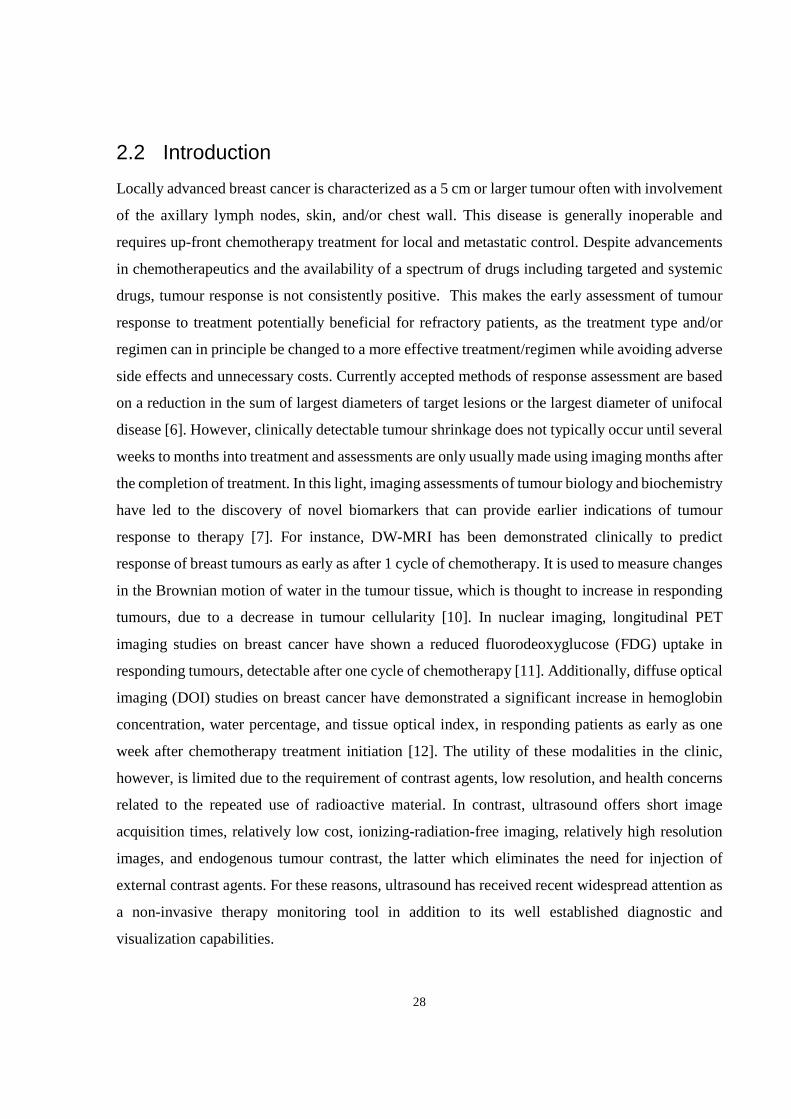
2.2 Introduction

Locally advanced breast cancer is characterized as a 5 cm or larger tumour often with involvement

of the axillary lymph nodes, skin, and/or chest wall. This disease is generally inoperable and

requires up-front chemotherapy treatment for local and metastatic control. Despite advancements

in chemotherapeutics and the availability of a spectrum of drugs including targeted and systemic

drugs, tumour response is not consistently positive. This makes the early assessment of tumour

response to treatment potentially beneficial for refractory patients, as the treatment type and/or

regimen can in principle be changed to a more effective treatment/regimen while avoiding adverse

side effects and unnecessary costs. Currently accepted methods of response assessment are based

on a reduction in the sum of largest diameters of target lesions or the largest diameter of unifocal

disease [6]. However, clinically detectable tumour shrinkage does not typically occur until several

weeks to months into treatment and assessments are only usually made using imaging months after

the completion of treatment. In this light, imaging assessments of tumour biology and biochemistry

have led to the discovery of novel biomarkers that can provide earlier indications of tumour

response to therapy [7]. For instance, DW-MRI has been demonstrated clinically to predict

response of breast tumours as early as after 1 cycle of chemotherapy. It is used to measure changes

in the Brownian motion of water in the tumour tissue, which is thought to increase in responding

tumours, due to a decrease in tumour cellularity [10]. In nuclear imaging, longitudinal PET

imaging studies on breast cancer have shown a reduced fluorodeoxyglucose (FDG) uptake in

responding tumours, detectable after one cycle of chemotherapy [11]. Additionally, diffuse optical

imaging (DOI) studies on breast cancer have demonstrated a significant increase in hemoglobin

concentration, water percentage, and tissue optical index, in responding patients as early as one

week after chemotherapy treatment initiation [12]. The utility of these modalities in the clinic,

however, is limited due to the requirement of contrast agents, low resolution, and health concerns

related to the repeated use of radioactive material. In contrast, ultrasound offers short image

acquisition times, relatively low cost, ionizing-radiation-free imaging, relatively high resolution

images, and endogenous tumour contrast, the latter which eliminates the need for injection of

external contrast agents. For these reasons, ultrasound has received recent widespread attention as

a non-invasive therapy monitoring tool in addition to its well established diagnostic and

visualization capabilities.

29

One of the ultrasonically detectable markers of tumour response is apoptotic cell death. The first

QUS studies of cell death induced by a chemotherapeutic agent demonstrated in vitro, that cell

death causes an increase in ultrasound echogenecity [53], [54]. These ultrasonic changes were later

quantified by system-independent parameters including integrated backscatter coefficient (IBSC),

MBF, and SS, all of which demonstrated an increase as a result of cell death [55]. This observation

was experimentally determined to be related to the nuclear condensation and fragmentation that

occur during apoptosis. The same ultrasonic pattern was observed in animal cancer models in vivo,

which indicated significant increases in MBF and SS resulting from photodynamic therapy [25],

or radiation therapy [26] of mouse tumour xenografts. More recently, a study on the low frequency

(7 MHz) QUS assessment of an animal model of breast cancer treated with chemotherapy

demonstrated that increases in the MBF and SI, but not SS, are strongly correlated to increases in

cell death [27]. The MBF, SI, and SS parameters have been used in the past for other tissue

characterization purposes, including the detection of prostate cancer, malignancies in lymph nodes,

uveal melanoma, and liver disease [12] – [15]. By modelling the ultrasonic power spectrum as a

linear approximation of the acoustic impedance autocorrelation, Lizzi et al. demonstrated that the

SS is related to the scatterer size, SI is related to scatterer size and acoustic concentration, and

MBF is related to the scatterer size, acoustic concentration, and attenuation [17]. Furthermore, the

fitting of advanced form factor models to ultrasonic tissue backscatter has permitted the direct

estimation of scattering properties of tissues, including average scatterer diameter ASD and AAC.

A form factor is proportional to the Fourier transform of the spatial autocorrelation of the relative

acoustic impedance between the scatterer and the background. The AAC parameter is a product of

scatterer number density and the acoustic impedance of the scatterers relative to the background.

These parameters have been demonstrated to be useful in differentiating between tumour types in

vivo, including sarcoma versus carcinoma [57], and carcinoma versus fibroadenoma [21]. More

recently, a clinical QUS study demonstrated significant increases in AAC in breast tumours of

patients who responded well to chemotherapy treatment, compared to those who did not respond

well, as early as one week after the start of treatment [23].

Various form factor models have been developed to describe tissue scattering, including the

spherical Gaussian model (SGM) and the fluid-filled sphere model (FFSM) [31]. The SGM

describes random scattering and a continuous variation of acoustic impedance between the

scatterer and its surrounding, and whose impedance autocorrelation follows a Gaussian curve. In

30

contrast, the FFSM describes scattering by randomly distributed fluid-filled spheres, in which the

cell nuclei are considered scatterers and the cytoplasm and the extracellular material are assumed

to be background material. Good fits have been observed with both models depending from which

kind of tissue ultrasound data is being obtained. Regardless, extensive evidence demonstrates that

nuclear material contributes to backscattered ultrasound signals. There are multiple sources of

experimental evidence suggesting the role of nuclear structure in potentially influencing

significantly ultrasound backscatter signals. This evidence spans work in vitro, cellular

experiments with cellular structure modifying agents, investigations of different cell types with

different nuclear sizes, and work with isolated nuclei from viable and apoptotic nuclei [45], [53],

[58].

In the work that has been examined to date on QUS detection of cell death, most experiments have

been conducted at high ultrasound frequencies (above 20 MHz), and those conducted at lower

ultrasound frequencies (<10 MHz) have used linear regression-based spectral analysis. At

frequencies above 20 MHz, tissue penetration depth is affected by attenuation and primarily small-

animal imaging has been performed. Clinical ultrasound imaging techniques employ linear array

transducers operating at a lower frequency range (1-10 MHz), which more readily permit imaging

of deeper tissue structures in breasts, kidneys, and livers, but with lower resolutions (150 µm – 1.5

mm). In addition, linear regression spectral analysis relies on a linear frequency dependence of the

tissue power spectrum over the usable frequency range, which may not be appropriate for some

tissues. On the other hand, solving the inverse scattering problem (i.e. estimating the scattering

properties from knowledge of the backscattering model and the measured backscatter) permits

direct estimation of scattering properties which may better reflect tissue composition, thereby

permitting a comparison of scatterer property estimates with underlying tissue microstructure. If a

set of acoustic parameters sensitive to cell death can be extracted from in vivo tumours using low

frequency ultrasound, this makes potentially possible the non-invasive ultrasound monitoring of

patients undergoing anti-cancer treatments.

Recently, several QUS parameters including means and texture features of MBF, SS, and SI and

envelope statistics parameters were investigated as potential biomarkers of cell death in vivo [27].

However, in that study, one in situ end labeling (ISEL)-stained histology image from the central

cross-section of the tumour was used to evaluate cell death extent, whereas QUS parameters were

evaluated from multiple sections across the tumour. To obtain a better correspondence between

31

histology and ultrasound, I examined cell death extent from five ISEL sections across the tumour

and from 5-10 ultrasound planes, I evaluated the corresponding ultrasound scattering properties of

tumours undergoing cell death by estimating advanced parameters from factor-based scattering

models. In addition, this study also examined the heterogeneity indicies (HIs) of AAC and ASD

(the standard deviations of AAC and ASD images) and initial tumour volume (Vi) as potentially

contributing factors to cell death response.

The overall objective of this study was to determine the optimal scattering model for estimating

scattering properties of mouse models of breast tumours (SGM or FFSM) based on goodness of fit

and scatterer size estimates, and using the optimal model’s parameters to track their time-

dependent cell death responses. Volumetric RF data were examined from human breast tumour

xenograft-bearing mice which were treated with chemotherapy. In order to determine which model

to use for scatterer properties estimation, two models, the SGM and the FFSM, were applied and

compared in terms of ASD agreement with histological features, goodness-of-fit of the models to

measured backscatter data, and the correlation of the extracted parameters to histologically

determined cell death extent. Backscatter coefficients from tumour regions of interest (ROI) were

estimated before and after treatment and form factor-based BSCs were fitted to the measured BSC

to estimate ASD and AAC parameters. Statistical tests were performed to compare changes in

ASD and AAC related to treatment against those related to tumour progression in control tumours.

Multiple regression analyses were performed on changes in ultrasonic scattering properties and the

extent of cell death observed histologically.

2.3 Methods

2.3.1 Experimental procedures The experimental protocol was approved by the institution's animal care committee for humane

and ethical use of laboratory animals. Human breast cancer cell line tumours (MDA-MB231,

American Type Culture Collection, Manassas, Virginia, USA) were established by injection of 1

× 106 cells in 50 µL of PBS into the hind legs of severe combined immunodeficiency disease

(SCID) mice and were permitted to grow to ~1 cm solid tumours. During treatment and imaging,

mice were anaesthetized with 100 mg/kg ketamine, 5 mg/kg of xylazine and 1 mg/kg of

32

acepromazine (CDMV, St. Hyacinthe Quebec, Canada). Chemotherapeutic agents Paclitaxel and

Doxorubicin (100mg/m2, 50mg/m2, respectively) were injected intravenously through the tail.

Pulse-echo imaging was performed prior to injection and a predetermined amount of time after

injection. Experimentation used 20 animals equally divided into 5 groups (n=4). The first 4 groups

were the treatment groups with 4, 12, 24, and 48 hours of wait time after chemotherapy injection,

respectively, and the fifth group served as untreated control tumours. Low and high-frequency

ultrasound data were acquired using two imaging systems - a Sonix RP system (Sonix RP,

Ultrasonix, Vancouver, Canada) operating a 7 MHz linear array transducer (L14-5/38) focused at

1.5 cm depth, with data sampled at 40 MHz, and a Vevo 770 system (Visual Sonics, Toronto,

Canada) utilizing a 20 MHz transducer (RMV-710B) focused at 9 mm depth, and sampled at 420

MHz. Both systems were used to collect volumetric data with scan plane separations of ~0.5 mm

in the conventional-frequency ultrasound and ~0.1 mm in the high-frequency ultrasound,

depending on the size of the tumour. Tumour volumes were estimated by approximating the

tumour volume as an ellipsoid and measuring the three axes (2a, 2b, and 2c) from in vivo three-

dimensional B-mode images obtained using the high frequency ultrasound system, and using the

formula (�f�� to estimate the volume. The images obtained from the high frequency system were

used for anatomical measurements since that system provided high resolution tumour images and

more accurate tumour delineation.

2.3.2 Quantitative ultrasound analysis For analyses, rectangular ROIs were selected from 5-10 tumour cross sections. These ROIs

accounted for approximately 2/3 of the tumour cross sectional area in ultrasound images

(approximately 5-10 × 5-10 × 5-10 mm). A sliding window analysis was performed on each ROI

using Hanning-gated RF windows of 2 × 2 mm size for low frequency data, and 0.62 × 0.62 mm

size for high frequency data, with 80% overlap between adjacent windows in both axial and lateral

directions. The axial length of the RF segments were selected to cover approximately 10

wavelengths, which corresponded to the minimum size required to obtain reliable spectral

estimates which are independent of window length (10 wavelengths) [59]. Each window spanned

13 RF scan lines in the low-frequency images and 11 RF scan lines in high-frequency images,

respectively. The mean sample power spectrum of each RF window was computed by taking the

squared magnitude of the FFT of the gated RF signal from every scan line and averaging the result

across the scan lines. The normalized power spectrum, 6(!), was obtained using the reference

33

phantom technique (equation 1.5). Spectral normalization removes system-dependent effects such

as transducer transfer function, beam forming, and diffraction artifacts. The reference material

used for spectral calibrations was a well characterized phantom consisting of glass microspheres

(5-40 µm) embedded in agar gel. The phantom was loaned from The Bioacoustics Research

Laboratory, University of Illinois at Urbana-Champaign, for which details are available in the

literature (phantom F1, table 2, in [60]). The reference BSC, #$5 , was measured using pulse-echo

technique and planar reflector (plexiglas) calibration, using equation 1.13, and was cross-verified

with the theoretical solution (see Appendix, p. 101). The measurement agreed with the theory (Fig.

7 of [60]). The estimated sample BSC, #$n, was obtained using the reference phantom technique

(equation 1.14). The SGM model (equation 0) was selected as the BSC model, for which #$

functions were calculated for a range of candidate scatterer radii (1-200µm). Scatterer properties,

including ASD and AAC, were estimated through MASD fitting of #$ onto #$n. This method was

described in section 1.6. The attenuation coefficient of the phantom was 0.15 dB/cm-MHz, which

was determined through an insertion-loss experiment and fitting a straight line through the

attenuation versus frequency data over the two system bandwidths (3-9 MHz and 10 – 25 MHz)

[44]. The normalized power spectrum was then compensated for frequency-dependent attenuation

using the point-by-point compensation method [31], assuming published attenuation coefficients

of 2 dB/cm/MHz and 0.6 dB/cm/MHz for skin [61] and tumour [26], respectively. Two QUS

features were defined from the parametric images of ASD and AAC – mean and heterogeneity

index (HI). HI was defined as the standard deviation of the parametric image, as per Nam et al

[22]. For comparison with cell death extent, changes in mean ASD and AAC (∆ASD, ∆AAC),

and changes in HI of ASD and AAC (∆HIASD, ∆HIAAC) before and after treatment administration

were considered. The mean coefficient of determination, <R2>, which indicates the goodness of

fit between measured and a theoretically derived backscatter coefficient was also calculated.

Finally, QUS parametric images were constructed by superimposing colored pixels, whose colors

were associated with QUS parameter estimate values and locations associated with the sliding

window locations, on the original grey scale B-mode image of the tumour [34].

2.3.3 Histology analysis Histology analysis was performed on excised tumour sections which were fixed in 5% formalin

(volume/volume) in PBS. Each fixed specimen was sectioned into five slices stained for

hematoxylin and eosin (H & E) and five slices stained for ISEL, with 50µm spacing. The cell death

34

fraction (CDF) of each tumour was determined, using ImageJ (National Institutes of Health,

Bethesda, MD) by manually contouring the ISEL-positive (brown stain) area and the total tumour

area and taking the ratio of the two areas. The mean CDF for each tumour was obtained by

averaging the CDFs from all the five sections. High-magnification images were obtained using a

Leica DC100 microscope with a 40× objective and a Leica DC100 camera connected to a 2-GHz

PC running Leica IM1000 software (Leica GmbH, Wetzlar, Germany). Areas which were

identified as ISEL-positive for CDF calculation were verified under high-magnification to contain

more than 50 % apoptotic cells. Mean cell and nucleus sizes were estimated by manually

measuring the diameters of approximately 100 cell / nucleus samples in the ISEL-stained sections

under high magnification.

2.3.4 Statistical Analysis

In order to evaluate of the goodness of fit of each form factor model, the mean coefficient of

determination, <R2>, was computed from all untreated tumours. To determine whether the changes

in the ASD/AAC parameters of treated tumours were statistically significantly different from those

of untreated tumours, t-tests (unpaired, two-tailed, α=0.05) or Mann-Whitney tests (α=0.05) were

applied to the data, depending on the distribution type. A p-value less than 0.05 was considered to

be statistically significant. Prior to performing hypothesis tests, a Shapiro-Wilk normality test was

first performed on the data to determine whether to use a parametric test (t-test) or non-parametric

test (Mann-Whitney). The correlations between CDF and BSC parameters were evaluated using

multiple linear regression analysis. The Pearson product-moment correlation coefficient, r2 metric,

was used to evaluate the strength of the correlation. For analysis of correlation between QUS and

histology (CDF), two scenarios were considered: multiple regression analysis on the set (∆AAC,

∆ASD, ∆HIAAC, ∆HIASD), and multiple regression analysis on the set (∆AAC,∆ASD, ∆HIAAC,

∆HIASD, Vi). The second scenario examined the effect of initial tumour volume on the BSC

parameters and hence on the prediction of cell death response.

35

2.4 Results

2.4.1 Histological assessment of treatment effects

Figure 2-1 presents H&E and ISEL stained sections of representative control and treatment time

groups. Whereas control tumours were characterized by multiple distinct nucleoli-containing cells

and microvessels, treated tumours were characterized by loss of microvessels, a decrease in the

number of cells with distinct nucleoli and increase in the number of cells with condensed nuclei in

H&E sections, and treated tumours also demonstrated an increase in areas of brown stains in the

extracellular space in ISEL sections. The strong focal stains in the H&E and blue-brown focal

stains in the ISEL sections were consistent in appearance with the nuclear condensation stage of

apoptosis and the brown stains in the extracellular space in the ISEL were consistent with the

appearance of fragmented DNA and cellular debris associated with the late stages of apoptosis.

Both H&E and ISEL sections indicated that as time progresses from 0 to 24 hours after the onset

of chemotherapy, tumours changed from a heterogeneous mixture of dead and viable cells to an

almost homogeneous tissue of dead cells. At 48 hours, tumours appeared to have entered the final

stages of cell death marked by nuclear degradation, as evident from a loss of cells with visible

nuclei. The mean changes in cell and nucleus size with treatment time are presented in Figure 2-1E.

In general, reductions in cell and nucleus size were observed resulting from chemotherapy as time

progressed, apparently plateauing at 48 hours. Plots of mean cell death fraction versus treatment

condition are presented in Figure 2-1F. Analysis of cell death obtained from ISEL-stained

histology images revealed a monotonic increase in cell death with time from treatment onset,

peaking at 24 hours, after which cell death dropped, but remained higher than cell death observed

in controls. The CDF was statistically significantly increased at 24 hours and 48 hours, compared

to the control group (unpaired t-test, p<0.05).

36

E F

Figure 2-1. (A-D) Histology images of representative control, 4-hour, 12-hour, 24-hour, and 48-hour chemotherapy-treated MDA-231 tumours, from left to right, respectively. (A) Low-magnification H&E stained sections. (B) Low-magnification ISEL stained sections (C) High-magnification H& E stained section to highlight nuclear material. (D) High-magnification ISEL section to highlight fragmented DNA. The control tumour features rapidly dividing cells with large nuclei. The treated tumours feature reduced nuclear size (nuclear condensation), fragmented nuclei, and dead cellular components filling the extracellular space (brown stains). The low-magnification scale bar represents 1 mm. The high-magnification scale bar represents 25 µm. (E) Plots of mean cell and nucleus diameters versus treatment time (0 to 48 hours), estimated from H& E histology sections. Error bars represent standard error of the mean. (F) Plot of the mean cell death fractions versus time. Error bars represent the standard error across the tumour samples for each time condition. Statistical significance: * = p<0.05.

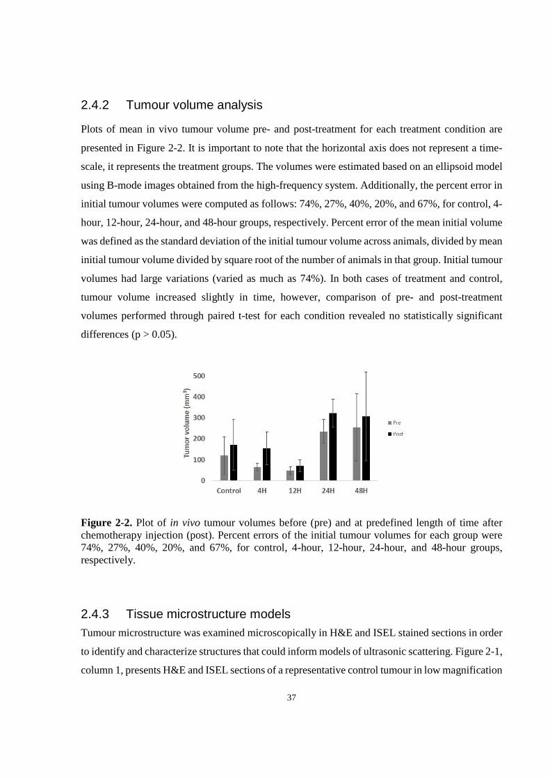
37

2.4.2 Tumour volume analysis

Plots of mean in vivo tumour volume pre- and post-treatment for each treatment condition are

presented in Figure 2-2. It is important to note that the horizontal axis does not represent a time-

scale, it represents the treatment groups. The volumes were estimated based on an ellipsoid model

using B-mode images obtained from the high-frequency system. Additionally, the percent error in

initial tumour volumes were computed as follows: 74%, 27%, 40%, 20%, and 67%, for control, 4-

hour, 12-hour, 24-hour, and 48-hour groups, respectively. Percent error of the mean initial volume

was defined as the standard deviation of the initial tumour volume across animals, divided by mean

initial tumour volume divided by square root of the number of animals in that group. Initial tumour

volumes had large variations (varied as much as 74%). In both cases of treatment and control,

tumour volume increased slightly in time, however, comparison of pre- and post-treatment

volumes performed through paired t-test for each condition revealed no statistically significant

differences (p > 0.05).

Figure 2-2. Plot of in vivo tumour volumes before (pre) and at predefined length of time after chemotherapy injection (post). Percent errors of the initial tumour volumes for each group were 74%, 27%, 40%, 20%, and 67%, for control, 4-hour, 12-hour, 24-hour, and 48-hour groups, respectively.

2.4.3 Tissue microstructure models Tumour microstructure was examined microscopically in H&E and ISEL stained sections in order

to identify and characterize structures that could inform models of ultrasonic scattering. Figure 2-1,

column 1, presents H&E and ISEL sections of a representative control tumour in low magnification

38

and high magnification views. In the H&E sections, tumours appeared to be predominantly

composed of tumour cells (purple-stained nuclei), with infrequent microvessels (red-pink stained),

and connective tissue (cyan-pink stained). Microvessels were only sparsely observed and had a

size of 20 ± 2 µm. The tumour cells dominated the tumour tissue. Both the H&E and ISEL sections

show densely packed cells with high mitotic indices and large nuclei (18 ± 3 µm diameter),

containing visible nucleoli. Table 2-1 lists the average cell size (histology), ASD, AAC, and mean

R2 (<R2>) goodness of fit values obtained from all pre-treated tumour BSC at low and high

frequencies using both models. Pre-treatment data was used because it permits the characterization

of MDA tumours in terms of scattering properties without the necessity to consider complex tissue

microstructures which can result from cell death. At the lower frequency range, both models

yielded large ASD values (109 ± 12µm for SGM, 95 ± 9µm for FFSM, p < 0.05). However, the

SGM provided a better fit to the measured backscatter data (<R2> = 0.21) compared to the FFSM

(<R2> = 0.07). For this reason, the SGM was used going forward and multiple linear regression

analysis was performed using ASD and AAC features extracted from this model. For the high-

frequency data, both models provided smaller ASD estimates (45 ± 7 µm for SGM and 38 ± 1 for

the FFSM), and the FFSM yielded a statistically significantly smaller ASD compared to the SGM

(p > 0.05). AAC can take on negative values, since it is expressed in dB/cm3. The dB units arise

from the logarithm applied to the BSC before MASD fitting is performed. The appropriateness of

the SGM and FFSM models for representing MDA tumour backscatter characteristics may at first

appear concerning due to the low <R2> values. This is due to the tumour heterogeneity, resulting

in a highly heterogeneous R2 distribution over the tumour volume, as demonstrated in Figure 2-3.

The tumour ROI contains regions of good fit and regions of poor fit. As shown, the best model fit

does not always occur in the center of the tumour, but sometimes in the periphery, in this case, the

best fit occurred in the lower limb. Additionally, Figure 2-3B demonstrates that the use of a larger

RF window size (3×3mm) results in higher R2 values as compared to 2×2mm window size used in

this study (Figure 2-3A). However, since 3×3mm was too large to fit in some of the smaller

tumours, I used 2×2mm as the standard window size. In the discussion section, an explanation will

be provided for why reasonable scatterer size estimates can be obtained regardless of low R2

values.

39

Table 2-1. Comparison of ASDs (µm) and AACs (dBr/cm3) estimated using the SGM and FFSM models at low and high frequencies (LF and HF) with mean histological measurement of tumour cell size. R2 is a measure of the goodness-of-fit of the model BSCs to the measured BSCs. ± represents standard deviations of the parameter over the tumour samples. Estimates were obtained from all tumours prior to treatment.

Cell diameter (µm)

18 ± 3

SGM FFSM

ASD AAC R2 ASD AAC R2

7 MHz 109 ± 12 5 ± 9 0.21 95 ± 9 7.35 ± 9 0.07

20 MHz 45 ± 7 32 ± 19 0.08 38 ± 1 -11 ± 11 0.06

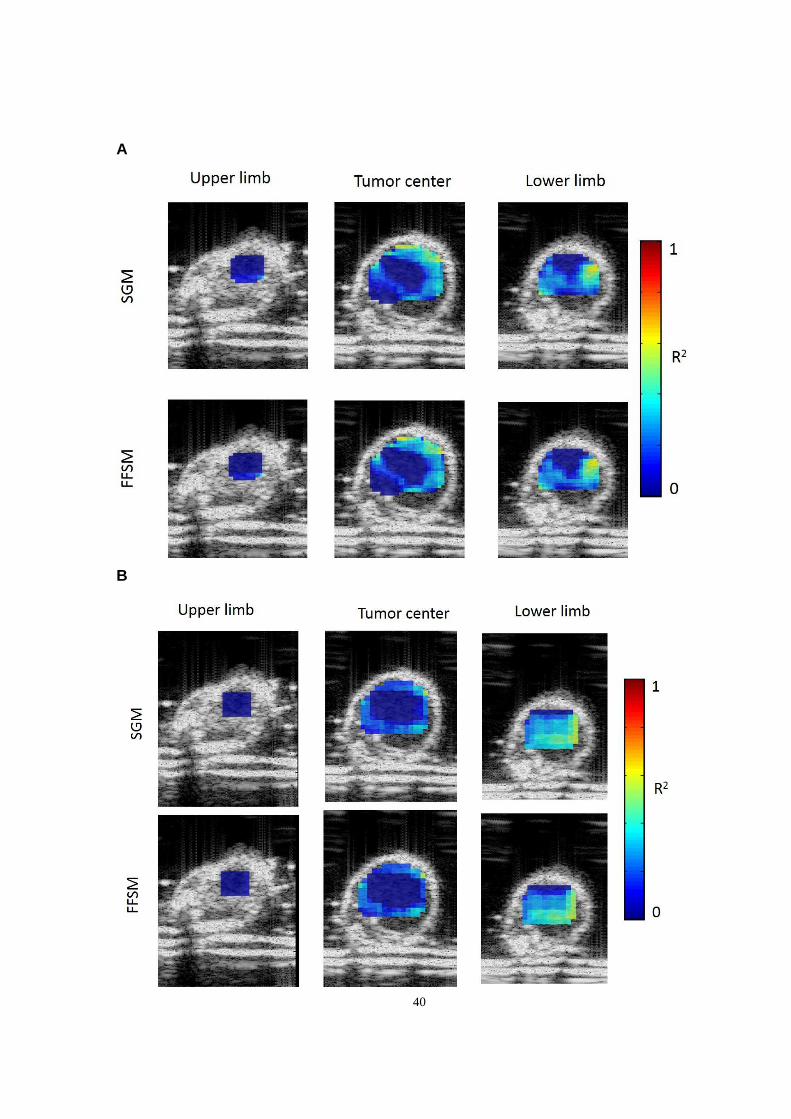
40

A

B

41

Figure 2-3. Illustration of the spatial distribution of R2 goodness of fits of the SGM and FFSM models over different tumour areas. Presented are R2 images overlaid on analyzed tumour ROIs over three tumour cross-sections: upper limb, tumour center, and lower limb. Data is presented from the low-frequency study with (A) 2 × 2 mm RF windows and (B) 3 × 3 mm RF windows.

Figure 2-4 presents combined low and high frequency plots of measured BSC and corresponding

theoretical BSCs based on the SGM and FFSM models obtained from one of the treated tumours.

The BSCs were obtained from an RF window at the center of the tumour ROI at low and high

frequencies. Results are shown before and 24-hours after chemotherapy injection. R2 values

ranged from 0.55 to 0.71. The FFSM model provided a better fit at high frequency at pre-treatment

whereas no considerable model differences were observed post-treatment. These values were

higher compared to the values reported in Table 2-1, because Table 2-1 eports the mean of mean

R2 where R2 was averaged across all windows in the tumour ROI and then across all pre-treatment

tumours. However, the R2 reported in Figure 2-4 were obtained from one RF window from one

animal. Generally, I observed lower R2 values in more heterogeneous tumours. An increase in the

BSC magnitude can be observed from pre-treatment to post-treatment at both frequency ranges.

This trend is consistent with the trend observed in AAC, which will be demonstrated in the next

section.

42

Figure 2-4. Combined low and high frequency plots of measured BSC and theoretical BSCs based on the SGM and FFSM models obtained from an animal in the 24-hour treatment group. Left: pre-treatment. Right: post-treatment. The BSCs were obtained from an RF window at the center of the tumour ROI. Corresponding R2 goodness of fit values are shown below the plots.

2.4.4 Ultrasonic scattering properties of cell death

Figure 2-5A-B presents AAC and ASD images obtained using the SGM from high and low-

frequency ultrasound imaging, respectively. The corresponding ISEL section post-treatment is also

presented. The cytotoxic effect of the treatment could be readily visualized in the ISEL section

(Figure 2-5C), demonstrating predominantly brown stained areas indicative of cell death. The

AAC images demonstrated that AAC increases considerably as a result of cell death (statistically

significant) at both frequencies, whereas the ASD was less sensitive to cell death at both

frequencies.

Figure 2-6A presents mean changes in AAC corresponding to different treatment conditions

(control, 4, 12, 24, and 48 hours) obtained from low and high-frequency RF data. Results

demonstrated a parallel trend in the AAC changes with treatment conditions as did the CDF in

Figure 2-1F. Initial observations suggested that AAC nominally increased proportionally with

time, peaking at 24h, following the observations for CDF. However, an unpaired t-test revealed

no statistical difference in AAC changes between 4 hours and the control groups, between 12 hours

and control group, and between 48 hours and the control group. Rather, a statistically significant

change could be detected only after 24 hours for both the low-frequency and high frequency data

(p = 0.003 and 0.043, respectively).

A stepwise multiple linear regression analysis of CDF versus BSC parameters (∆AAC, ∆HIAAC,

∆ASD, ∆HIASD) revealed the single-most correlated parameter to be ∆AAC with a correlation (r2)

of 0.399 and the most correlated multiparameter QUS model to be a linear combination of ∆AAC

and ∆HIASD with a correlation of 0.639, as presented in Table 2-2. Furthermore, when initial tumour

volume (Vi) was added to the model on the working hypothesis that biological changes in tumour

structure associated with tumour growth may affect data, the correlation further increased to 0.744

(Table 2-2). Presented in Table 2-2, column 3, are p-values of significance of one-way ANOVA

tests, demonstrating the statistical significance of the correlations between CDF and each

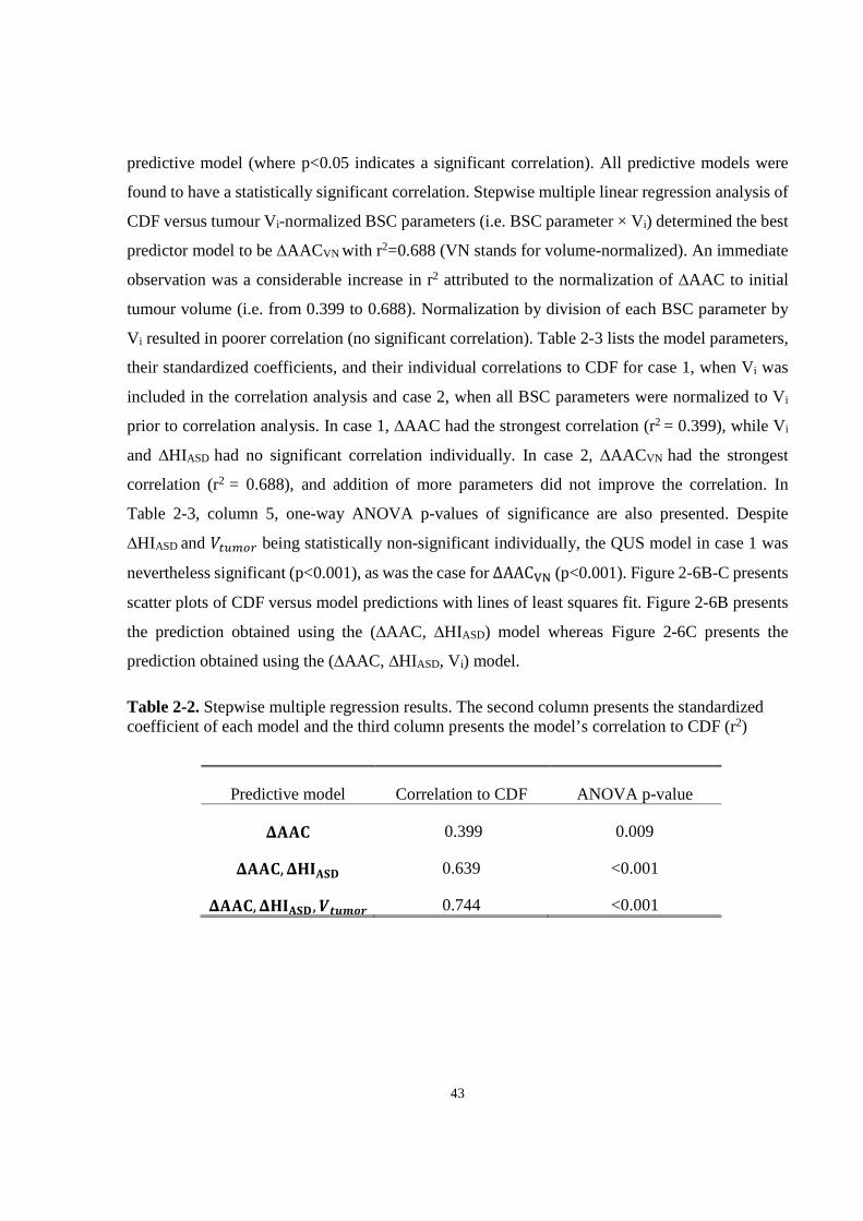
43

predictive model (where p<0.05 indicates a significant correlation). All predictive models were

found to have a statistically significant correlation. Stepwise multiple linear regression analysis of

CDF versus tumour Vi-normalized BSC parameters (i.e. BSC parameter × Vi) determined the best

predictor model to be ∆AACVN with r2=0.688 (VN stands for volume-normalized). An immediate

observation was a considerable increase in r2 attributed to the normalization of ∆AAC to initial

tumour volume (i.e. from 0.399 to 0.688). Normalization by division of each BSC parameter by

V i resulted in poorer correlation (no significant correlation). Table 2-3 lists the model parameters,

their standardized coefficients, and their individual correlations to CDF for case 1, when Vi was

included in the correlation analysis and case 2, when all BSC parameters were normalized to Vi

prior to correlation analysis. In case 1, ∆AAC had the strongest correlation (r2 = 0.399), while Vi

and ∆HIASD had no significant correlation individually. In case 2, ∆AACVN had the strongest

correlation (r2 = 0.688), and addition of more parameters did not improve the correlation. In

Table 2-3, column 5, one-way ANOVA p-values of significance are also presented. Despite

∆HIASD and ���l�5 being statistically non-significant individually, the QUS model in case 1 was

nevertheless significant (p<0.001), as was the case for ΔAAC�� (p<0.001). Figure 2-6B-C presents

scatter plots of CDF versus model predictions with lines of least squares fit. Figure 2-6B presents

the prediction obtained using the (∆AAC, ∆HIASD) model whereas Figure 2-6C presents the

prediction obtained using the (∆AAC, ∆HIASD, Vi) model.

Table 2-2. Stepwise multiple regression results. The second column presents the standardized coefficient of each model and the third column presents the model’s correlation to CDF (r2)

Predictive model Correlation to CDF ANOVA p-value

���� 0.399 0.009

����,������ 0.639 <0.001

����,������, ������ 0.744 <0.001

44

Table 2-3. Stepwise multiple regression results for the two cases - with and without tumour volume normalization (separated by a horizontal line). The second column presents the standardized coefficient of each parameter and the third column presents the parameter's correlation to CDF (r2). NS indicates non-significant results (p>0.05).

Case Predictive model

parameter Standardized Model

Coefficient Correlation to

CDF ANOVA p-value

Case 1 ���� 0.765 0.399 0.009 ������ 0.429 NS NS ��� ¡¢ 0.336 NS NS

Case 2 �����£ 0.829 0.688 <0.001

45

Figure 2-5. Pre- and post- treatment (24h) images of the central cross section of a sample MDA-231 tumour which received chemotherapy treatment. (A) and (B) show ASD and AAC images

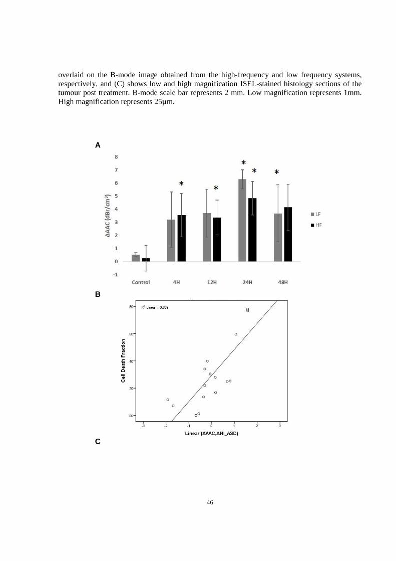
46

overlaid on the B-mode image obtained from the high-frequency and low frequency systems, respectively, and (C) shows low and high magnification ISEL-stained histology sections of the tumour post treatment. B-mode scale bar represents 2 mm. Low magnification represents 1mm. High magnification represents 25µm.

A

B

C

47

Figure 2-6. Results of QUS analysis of cell death. (A) Plot of ∆AAC versus time from treatment onset obtained using the low and high frequency systems. Error bars represent the standard error across the tumour samples for each time condition. Statistical significance: * = p<0.05. (B) Scatter plot of CDF versus the predictive model (∆AAC, ∆HIASD), r2=0.639. (C) Scatter plot of CDF versus the predictive model (∆AAC, ∆HIASD, and Vi ), r2 = 0.744.

2.5 Discussion and Conclusions

Ultrasound is widely preferred over currently available breast imaging modalities due to its

relatively low cost, high spatial and temporal resolution, safety, and independence from external

contrast agents. This study demonstrated that scattering properties can be potentially used as

biomarkers of treatment response-related cancer cell death, at high (20 MHz) and low (7 MHz)

ultrasound frequencies. Examination of tumour histopathology revealed clusters of tumour cells

and microvessels as dominant features which could serve as potential scatterers of ultrasound with

sizes of 18 ± 3 µm, and 20 ± 2 µm, respectively. Two scattering properties, ASD and AAC, were

estimated using the SGM and FFSM models. Analysis of ISEL-stained histopathology revealed a

progressive increase in cell death extent with time up to 24 hours from treatment initiation, after

which cell death decreased due to nuclear and cellular degradation (48 hours). Changes in AAC

related to cell death were consistent with changes in surrogate measures of AAC (i.e. MBF and

SI) that were assessed in previous works [26], [27], and changes in backscatter intensity observed

in previous in-vitro studies [54], [55]. In the study here, the use of a wider analysis bandwidth

permitted a better characterization of the frequency-dependent backscatter of treated and untreated

48

tumours, by fitting advanced scattering models as opposed to applying a simple linear regression

to the power spectrum within a narrow bandwidth. Physical insight into the link between low-

frequency scattering properties and underlying microstructure of the dying tumours was gained to

help explain previous QUS findings. It is likely that these findings stem from changes which

correspond to scattering from a mixture of microsvessels and larger tumour cell clusters.

Our working model of the ultrasonic scattering properties related to cell death is that nuclear

changes are responsible for the increase in AAC. Since AAC is the coefficient of the BSC, it is

related to the backscatter amplitude. Previous in vitro and in vivo studies suggest that changes in

the magnitude and frequency dependence of ultrasound backscatter with cell death arise from

coincident changes in the nuclear structure of the cell [25], [45], [53].

As tumour structure becomes more complex in association with tumour growth there are further

complexities which are linked to potential sources of ultrasound backscatter. The degree of fit

between the SGM and FFSM models and the measured BSC at both low and high frequency ranges

were consistent with the work of others (R2=0.1-0.3) [57]. These previous studies have also

demonstrated that the degree of model fit to the measured backscatter does not reflect the accuracy

of the scatterer size estimates (i.e. agreement between scatterer size and observed microstructure)

and models which fit the measurement with less than 0.50 <R2> can nevertheless estimate the

scatterer properties reasonably well [57].

The scattering models that were applied in this study were not used to characterize scattering by

individual cells, rather, it is hypothesized that clusters of tumour cells or microvessels were

detected as scatterers. Immunohistochemical examination of tumours 24 hours after therapy

exposure revealed positive staining covering nearly 60% of the tumour. Recall that AAC is related

to the product of scatterer number density and relative acoustic impedance. Thus, the observed

increases in AAC due to cell death may have been caused by changes in the acoustic impedance

of the scatterers relative to the background, since nuclear fragments and cellular debris filled the

extracellular space. For this reason potentially, AAC showed a stronger correlation to cell death

(R2SGM=0.40) compared to ASD (R2SGM was non-significant).

An important finding in this study was that initial tumour volume measurements demonstrated

large variations (as high as 74 % of the mean value). This variation was likely due to differences

49

in tumour growth. The correlation between ∆AAC and CDF improved when ∆AAC was

normalized to initial tumour volume (from 0.399 to 0.688) as this accounted for variations in initial

tumour volume and therefore any effects of tumour necrotic centers. As tumours grow beyond 7-

10 mm in our experience more vascularization occurs and also baseline levels of necrosis are

thought to arise from transient hypoxia. The reduction in cell size observed histologically and

associated with cell death could not be detected by scatterer property estimates, as the ASDs

estimated by both models were considerably larger than cells (5 times larger at low frequency and

2 times larger at high frequency). In a tumour study, comparing three form factor models for

characterizing mammary carcinoma and sarcoma tumours in mouse models, Oelze et al.

demonstrated that the SGM best predicts the size of cell scatterers, although the FFSM provided

better fits to the backscatter power [57]. In contrast, the high-frequency backscatter data here were

fitted better with the SGM model. This suggests that depending on the tumour type, the SGM

model may also describe scattering by an aggregate of cells, rather than individual cells, as was

previously hypothesized by Oelze et al. [57].

Analysis of changes in AAC with treatment indicated greater increases in AAC estimated from

low-frequency data compared to those estimated from high-frequency data, after 24 hours (nearly

2 dBr higher). This observation was consistent with previous findings in-vitro: in the 10-30 MHz

range, cell samples treated with chemotherapy demonstrated a 5 dBr increase in backscatter

amplitude, while in the 30-50 MHz range, a lesser 2 dBr increase was observed [62].

Multiple regression analysis of QUS versus CDF demonstrated the “best” single parameter based

on the experiments conducted to be ∆AAC and the “best” multiparameter model to be ∆AAC,

∆HIASD, and Vi. It is believed that ∆HIASD reflects changes in heterogeneity of the tumour in

response to therapy. The improvement obtained by adding Vi to the regression model suggests that

initial tumour volume affects the BSC parameters and CDF and is an important parameter. The

rationale is that larger tumours often develop necrotic and/or hypoxic regions which could

potentially alter the acoustic scattering properties.

In a recent clinical QUS study which examined changes in AAC and ASD estimated from the

FFSM fitting of the BSC from patient breast tumours, significant increases in AAC were observed

as early as one week after the start of treatment [23]. However, no corresponding histopathological

data was available during the treatment to compare AAC changes with microstructural changes in

50

the tumour. Rather, AAC changes measured during the treatment were compared with clinical

response determined based on tumour size reduction at the end of the treatment which generally

lasts several months. The low-, and clinically relevant - frequency pre-clinical study performed

here, backed by high-frequency data, suggests that the increases in AAC observed clinically during

anti-cancer treatment, is likely associated with cell death response. However, the findings of this

study suggests that other factors such as tumour heterogeneity and initial tumour volume should

also be taken into account when assessing tumour response.

The fact that SGM form factor fitted the measured BSC better compared to the FFSM form factor

may owe to the theory that the SGM model better reflects the acoustic impedance autocorrelation

function of the tumour. As mentioned previously, form factors are proportional to the Fourier

transform of the spatial autocorrelation of the relative acoustic impedance between the scatterer

and the background. A continuous change in acoustic impedance between the scatterer and its

background, which is assumed in the SGM model, may better reflect the interface between tumour

cell clusters and the extracellular matrix, as opposed to a discrete change in acoustic impedance

described by the FFSM model.

In all, scatterer property-based QUS biomarkers, including ∆AAC, ∆HIASD, and Vi demonstrated

a favorable correlation to cell death extent (CDF). The results of this work are promising for the

development of QUS imaging methods for monitoring of breast tumour response to anticancer

therapy, requiring only a standard clinical US scanner equipped with QUS processing and imaging

software.

51

3 Quantitative ultrasound characterization of locally advanced breast cancer

52

3.1 Overview Purpose: Identification of tumour pathological characteristics is an important part of breast cancer

diagnosis, prognosis, and treatment planning, but currently requires biopsy as its standard. Here, I

investigated a non-invasive quantitative ultrasound method for characterization of breast tumours

in terms of their histological grade, which can be used with clinical diagnostic ultrasound data.

RF data from 57 locally advanced breast cancer patients were analyzed as part of this study. Among

these patients, 42 normal breast tissues and 42 breast tumours were selected for characterization

of normal versus cancer in the breast. For tumour grade characterization, 7 patients had grade I

tumours and 50 had grade II-III tumours. Six quantitative ultrasound parameters were

simultaneously extracted from tumour and normal breast tissue regions in the RF data, including

mid-band fit, spectral slope, 0-MHz intercept, scatterer spacing, average scatterer diameter, and

average acoustic concentration. For tumour grade characterization, a seventh parameter was

included in the analysis - attenuation coefficient estimate. Histopathological information from

breast biopsy was used to identify the tumour location(s) with the guidance of an oncologist during

the scans. Parametric maps were generated corresponding to the region of interest, from which

four textural features, including contrast, energy, homogeneity, and correlation were determined

as additional potential tumour characterization parameters. Data were examined on the basis of

tumour versus normal tissue and tumour subtypes based on histological grade (grade I versus grade

II-III).

Results: All six quantitative ultrasound parameters were found to be statistically different between

tumour and normal tissue (p < 0.05). The combination of average acoustic concentration and mean

scatterer spacing could separate tumour from normal tissue with 88% accuracy, while the addition

of effective scatterer diameter to the combination did not provide substantial improvement (89%

accuracy). For tumour grade characterization, linear discriminant analysis of the means of the

parametric maps resulted in classification accuracy of 79 %. On the other hand, the linear

combination of the texture features of the parametric maps resulted in classification accuracy of

82 %. Finally, when both the means and textures of the parametric maps were combined, the best

classification accuracy was obtained (86 %).

Conclusions: Textural characteristics of quantitative ultrasound spectral parametric maps provided

discriminant information about different types of breast tumours. In particular they significantly

improved the results of ultrasonic tumour characterization whereas conventional mean values used

alone tended to be poorer. As such, this study suggests that texture-based quantitative ultrasound

53

analysis of in-vivo breast tumours can provide complementary diagnostic information about

tumour histological characteristics.

3.2 Introduction An accurate diagnosis of breast tumours plays an important role in prognosis and therapy planning,

and can improve overall survival. X-Ray mammography is currently the primary imaging modality

for breast examinations. However, mammographic sensitivity declines substantially with

increasing breast density particularly in young women [63]. Clinical ultrasound, when performed

in conjunction with mammography, has been reported to increase diagnostic accuracy from 78%

to 91% [64]. However, due to the many instrument parameters that can be chosen during an

ultrasound imaging session, a comparative interpretation of conventional B-mode images becomes

difficult when different imaging settings are applied or when different ultrasound machines are

used. In addition, B-mode images, which are used by radiologists for breast examination, lack

readily accessible information about microstructural properties of soft tissues. This information is

lost when raw ultrasound data, or RF data, is converted to gray-scale pixels. QUS techniques,

which examine the frequency-dependence of backscatter from tissues (from analyzed RF data),

have been developed to overcome these limitations. Such techniques have been applied in vivo in

a variety of applications to reveal information about tissue microstructure, enabling the

differentiation of disease from non-disease, and the characterization of disease into its subtypes.

Applications include the characterization of tissue abnormalities, such as those in the eye, prostate,

and myocardium and to detect cancer in the lymph nodes [13]–[16]. Specifically, QUS parameters

including ASD and AAC (related to effective scatterer number density and relative acoustic

impedance) have demonstrated the potential to be used to distinguish between mouse models of

mammary carcinoma and rat models of fibroadenoma. These parameters can be obtained by fitting

a form factor model, such as the Gaussian form factor, to the measured backscatter coefficient

[34]. In order to avoid complex model fitting, basic spectral parameters extracted via a linear

regression analysis of the RF power spectrum, including MBF, SS, and SI, have also been used for

tissue characterization previously [13]–[16]. By modelling the ultrasonic power spectrum as an

acoustic impedance autocorrelation function, Lizzi et al. demonstrated that parameters, extracted

from a linear fit to the power spectrum within the usable frequency bandwidth, are related to the

scattering properties of the tissue of interest. In particular, they found that SS is related to effective

54

scatterer size, SI is related to effective scatterer size and acoustic concentration, and MBF is related

to effective scatterer size, acoustic concentration, and attenuation [18]. However, power spectrum

measurements are affected by the inherent frequency-dependent attenuation of intervening tissues,

requiring correction for accurate estimates of scattering properties.

Frequency-dependent attenuation has also been shown to be a useful parameter in characterizing

tissues, especially tumours and normal tissues of the breast [44]. Furthermore, a previous clinical

study found large variations in the ACE among breast tumours (1.16 ± 0.8 dB/cm/MHz),

suggesting different tumour types [22]. Another parameter, SAS, has been investigated as a tissue

characterization parameter when the tissue of interest contains detectable periodicity in its

structural organization. Previous studies have investigated the potential of SAS mainly for

characterizing diffuse diseases of the liver [38]–[40]. More recently, scatterer spacing has also

been applied to characterize human breast tumours in terms of normal breast tissue, fibroadenoma,

simple carcinoma, and infiltrating papillary carcinoma [42]. However, subtle differences were

found between the scatterer spacing values estimated from these tissue types.

Whereas the conventional quantitative ultrasound spectral parameters discussed above describe

the frequency-dependent properties of tissue microstructure, an analysis of textural characteristics

of QUS-based parametric maps can potentially provide second order statistics by quantifying the

patterns of gray-level transitions. Texture-based parameters carry high-order discriminative

information about patterns of neighbouring pixels in an image, and have been applied in the past

on B-mode ultrasound for discriminating between benign and malignant breast tumours [65], [66].

The principle behind this tissue classification technique is that malignant tumours tend to present

as heterogeneous internal echoes, whereas benign masses often demonstrate homogeneous internal

echoes. Textural analysis techniques aim at extracting the tissue internal echo properties or

"texture", based on the ultrasonic gray-level transitions, and hence can define differentiable

characteristics in this application. However, previous studies [65], [66] have used conventional B-

mode images for textural analysis, which may present undesirable variations in textural estimates

due to variations in instruments settings, ultrasound beam diffraction, and attenuation effects. Such

limitations can be addressed by performing texture analysis on quantitative ultrasound parametric

images for which these artefacts have been compensated. This method was first applied

successfully by Sadeghi-Naini et al. to characterize tumour cell death responses to chemotherapy

in vivo [27] and was adapted here to investigate more subtle differences in tumour characteristics.

55

This study investigates, for the first time, the capacity of the textural characteristics of quantitative

ultrasound parametric maps to characterize breast tumours comprehensively in terms of

differentiating from normal breast tissues and in terms of their histological grade. Applying

textural analysis on ultrasound spectral parametric maps rather than on B-mode images (as

employed in previous techniques by other investigators) allows for instrument-independent

characterization of tissues. Results here suggest that large tumours can be graded with 82%

accuracy using textural features of spectral parametric maps, and a further classification accuracy

of 88% can be obtained using the combination of means of the parametric maps and textural

parameters. Thus, this work paves the path for the development of a systematic computer-aided

breast tumour characterization methodology using non-invasive QUS techniques.

3.3 Methods

3.3.1 Overview

The breast tissue characterization technique used here was a two-stage process involving QUS

parameter estimation followed by classification. Given a tumour region of interest (ROI) in a breast

ultrasound image, QUS parameters including MBF, SS, SI, SAS, ASD, AAC, and ACE were

computed from its RF data. In addition to the mean of the parametric map, textural features

including contrast, correlation, energy, and homogeneity were determined from the parametric

map based on a gray level co-occurrence matrix (GLCM) [48].

A total of 31 parameters were considered for characterization: means from six parametric maps

(MBF, SS, SI, SAS, ASD, AAC), a single-value parameter (ACE), and four texture features per

parametric map (4 × 6 = 24 texture features in total). The Fisher linear classifier [67] was used to

classify tissues using different QUS parameter combinations. Finally, a leave-one-out analysis was

performed on the classification of grade I versus grade II-III tumours and metrics such as grade I

prediction rate, grade II-III prediction rate, accuracy, and area under the receiver-operator

characteristic curve were used to evaluate the classification results. The rationale for separating

grade I tumours from grade II and III tumours was that patients with grade I tumours are low-risk

patients compared to patients with grade II and III tumours, in terms of their management.

56

3.3.2 Ultrasound data acquisition and processing

LABC patients (N=57, NG1=7, NGII-III =50) were recruited in this study for non-invasive tumour

grading. For analysis of the QUS characteristics of breast tumours versus normal breast tissues,

the first 42 patients were analyzed (as the remaining 15 patients were analyzed at a later time) and

the results were reported in [24]. Patients with large tumours (3 cm or larger) were selected in this

study to avoid uncertainties in tumour identification. All information regarding histopathological

characteristics of the tumours, including type and grade, were determined from clinical biopsy

pathology reports. Tumour size was defined as the sum of the long axis lengths of the tumour foci

and was determined from diagnostic MR imaging reports. For performing supervised learning

using linear discriminant analysis, tumours were histologically divided into two classes - grade I

and grade II-III. This used the maximum number of available tumours in the study, since roughly

30 % of the tumours were identified by institutional pathologists as intermediate-to-high grade

rather than a definitive grade II or grade III. Radiofrequency and B-mode ultrasound data were

collected from the affected breast using a Sonix RP ultrasound scanner operating a 6 MHz-

stimulated broadband array transducer (L14-5/38, Ultrasonix, Vancouver, Canada). RF Data were

sampled at 40 MHz at a 512 line density, resulting typically in images with 6 cm width and 4-6

cm depth. Four to seven image planes of the tumour were selected at 1 cm intervals across the

affected breast for analysis. In the same scan, one cross-sectional image of the normal tissue region

of the breast was also obtained.

Regions-of-interest (ROIs) enclosing the central mass the tumour (approximately 90% of tumour

volume) were selected across four to seven tumour cross-sections, and a cross-section of normal

breast tissue was selected, under the guidance of an oncologist. The margins of the tumour were

excluded in order to avoid any ambiguities in the boundary definitions. Each ROI was then

segmented using a sliding window approach with 80 % overlap between adjacent windows. Each

window had dimensions of 2 mm by 2 mm. The size of the window was selected to cover

approximately 17 ultrasound wavelengths, larger than the minimum size (10 wavelengths)

typically required to obtain reliable spectral parameters which are independent of window length

[59].

In order to make the analysis method system-independent, processed US data were normalized on

a sliding-window basis using reference data obtained from a tissue-mimicking phantom or a planar

reflector. For linear regression analysis of the power spectrum, an in-house constructed tissue-

57

mimicking phantom was used, comprising of agar gel embedded with glass microspheres

(modified from [68]). For SAS analysis, a plexiglas planar reflector was used as reference, as SAS

estimation is sensitive to the spatial distribution of the scatterers in the reference medium, and a

planar reflector has relatively simpler scattering properties compared to that of the phantom used

in this study. Echo data from the polished plexiglas surface were obtained at 12 equally spaced

depths from 1 to 6 cm, which covered all possible breast tumour depths. For a given tumour

window, the corresponding reference window was selected by nearest neighbour interpolation.

The data normalization process is discussed in more detail below.

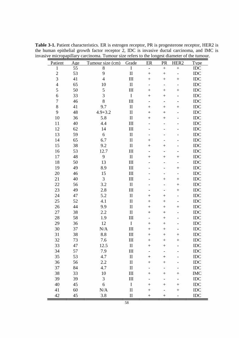
58

Table 3-1. Patient characteristics. ER is estrogen receptor, PR is progesterone receptor, HER2 is the human epithelial growth factor receptor 2, IDC is invasive ductal carcinoma, and IMC is invasive micropapillary carcinoma. Tumour size refers to the longest diameter of the tumour.

Patient Age Tumour size (cm) Grade ER PR HER2 Type 1 55 8 I - + + IDC 2 53 9 II + + - IDC 3 41 4 III + + + IDC 4 65 10 II - - - IDC 5 50 5 III + + + IDC 6 33 3 I + + - IDC 7 46 8 III - - - IDC 8 41 9.7 II + + + IDC 9 48 4.9+3.2 II + + - IDC 10 36 5.8 II + + - IDC 11 40 4.4 III - - - IDC 12 62 14 III - - - IDC 13 59 6 II - - - IDC 14 65 6.7 II + - - IDC 15 38 9.2 II + + - IDC 16 53 12.7 III - - - IDC 17 48 9 II + + + IDC 18 50 13 III - - - IDC 19 49 8.9 III - - + IDC 20 46 15 III - - - IDC 21 40 3 III - + + IDC 22 56 3.2 II - - + IDC 23 49 2.8 III - - + IDC 24 47 5.2 II + + - IDC 25 52 4.1 II + + - IDC 26 44 9.9 II + + + IDC 27 38 2.2 II + + - IDC 28 58 1.9 III - + - IDC 29 36 12 I + + - IDC 30 37 N/A III + + - IDC 31 38 8.8 III + + + IDC 32 73 7.6 III + + + IDC 33 47 12.5 II + + - IDC 34 57 7.9 III - - - IDC 35 53 4.7 II + + - IDC 36 56 2.2 II + + - IDC 37 84 4.7 II - - - IDC 38 33 10 III + + + IMC 39 39 3 III - - - IDC 40 45 6 I + + + IDC 41 60 N/A II + - + IDC 42 45 3.8 II + + - IDC

59

3.3.3 Quantitative ultrasound analysis

All analyses of frequency-dependent backscatter were carried out within the -6 dB system

transducer bandwidth, which was 3-8 MHz. The first step in the QUS analysis was computation

of the ACE of the tumour, which was required for attenuation correction of the tumour power

spectrum. The ACE was computed using the reference phantom method by estimating the rate of

change in the spectral magnitude with depth and frequency relative to a reference medium with a

known attenuation coefficient [46]. The reference medium was a well-characterized tissue-

mimicking phantom with known attenuation coefficient and speed of sound. Plots of relative

spectral amplitude versus depth were obtained by averaging the normalized window power spectra

across laterally adjacent windows and then plotting the average amplitude at each frequency

against the depth of the windows in the ROI. The ACE of the tumour was estimated by averaging

the slopes of the linear fits to the amplitude versus depth data at all frequency points in the

bandwidth. The newly found ACE was used to correct the tumour power spectrum for attenuation

using the point attenuation compensation method [47]. Afterwards, spectral parameters, including

MBF, SI, and SS were extracted from linear regression of the attenuation-corrected power

spectrum within the -6 dB bandwidth, using established spectral analysis methods [17].

Using the same attenuation-corrected power spectrum, the BSC of the tumour was estimated using

the reference phantom technique. Then, by MASD fitting of the Gaussian form factor to the BSC,

parameters of the Gaussian form factor, ASD and AAC, were determined, as described in section

1.6 of the thesis. The SAS parameter was computed using the AR model and the SAC technique,

as described in section 1.5 of the thesis.

3.3.4 Statistical textural analysis of quantitative ultrasound maps In this study, a statistical texture analysis technique was applied which is based on the concept of

GLCM. The GLCM represents, statistically, the angular relationship between neighbouring pixels

as well as the distance between them [48]. Based on the statistical information provided by GLCM

analysis, several textural features were determined including contrast (CON), correlation (COR),

homogeneity (HOM), and energy (ENE), as defined in equations 1.20, 1.21, 1.22,

and 1.231.211.22, respectively.

60

Parametric maps of MBF, SS, SI, SAS, ASD, and AAC each underwent a GLCM-based texture

analysis process in order to extract four textural features. Texture properties could not be extracted

from ACE, since a single value was computed from each ROI rather than computing a parametric

map, as a large number of points (depths) were required to obtain accurate estimates of attenuation

slope. In texture analysis, the contrast parameter represents a measure of difference between the

lowest and highest intensities in a set of pixels. The energy parameter measures the frequency of

occurrence of pixel pairs and quantifies its power (square of the frequency of gray-level

transitions). The homogeneity parameter measures the incidence of pixel pairs of different

intensities. As the frequency of pixel pairs with close intensities increases, homogeneity increases.

The correlation parameter measures the intensity correlation between pixel pairs. Sixteen

symmetric GLCMs were constructed for each parametric map, corresponding to four pixel-to-pixel

distances (1 pixel, 2 pixels, 3 pixels, and 4 pixels) and four directions (0˚, 45˚, 90˚, and 135˚). The

texture feature for each of the 16 symmetric GLCMs were computed and averaged to obtain a

mean texture value. This resulted in 24 mean textural features (four features for each of the six

parametric maps) which were subsequently applied, for distinguishing tumours from normal tissue,

as well as for characterizing the tumours into their grade.

3.3.5 Tissue classification algorithm Two levels of classifications were performed: tumour versus normal tissue, and grade I versus

grade II-III tumours. For tumour versus normal tissue classification, I performed multivariate

statistical analysis using the quadratic discriminant function. Combinations of ASD, AAC, and

SAS were tested, since these QUS parameters provide useful physical insight about tissue

microstructure and their means were found to be statistically different in tumours versus normal

tissue. For classification of tumour grades, linear discriminant analysis was performed by

employing sequential feature selection from the 31 QUS features (means and textures) and

performing leave-one-patient-out cross-validation. Cross-validation allows one to determine how

well the classification results generalize to an independent data set. The process involves dividing

the data set into training and testing sets and training the classifier using the training set, then

testing the classifier using the test set. The process is repeated until all data samples have been

tested. The classification performances were evaluated in terms of area under the ROC curve,

sensitivity, specificity, and accuracy.

61

3.4 Results

3.4.1 QUS analysis of tumour versus normal tissue Relevant patient characteristics, including age, tumour size, tumour type, grade, and hormone

receptor expressions (ER/PR/HER2) are summarized in Table 3-1. The patients had an average

age of 49 (SD = 11) with mean tumour size (longest diameter) of 7.5 cm (SD = 4 cm). Tumours

were predominantly of the invasive ductal carcinoma type (98%), with the exception of one case

of invasive micropapillary carcinoma.

Each of the QUS parameters underwent paired and unpaired tests in order to determine the

statistical significance of the difference between tumour and normal breast tissue ROI. A paired

test determined whether mean parameter values in tumour ROIs and normal breast tissue ROIs are

statistically significantly different, while maintaining the correspondence of the ROIs with the

patient. On the other hand, an unpaired test determined whether mean parameter values in tumour

ROIs and normal breast tissue ROIs are statistically significantly different, without accounting for

ROI-patient correspondence. This evaluated the inter-patient variations of the QUS parameters.

For MBF and ASD, paired/unpaired t-tests were performed between the tumour and normal tissue

groups, since the data passed the normality test. For SS, SI, SAS, and AAC, Wilcoxon/Mann-

Whitney (paired/unpaired) tests were performed to account for the non-normal distributions. These

tests resulted in (paired, unpaired) p-values of <0.0001,0.0001* (MBF), 0.0075,0.038* (SS),

0.0001,0.0008* (SI), <0.0001,0.0001* (SAS), 0.0042,0.0279* (ASD), and <0.0001,0.0001*

(AAC), comparing tumour to normal tissue. All six parameters demonstrated statistically

significant different means (p <0.05) between tumour and normal tissue, both in paired and

unpaired terms. In terms of class separation, however, there was a large overlap of the distributions

of the QUS parameters. To improve the class separation, I performed multivariate statistical

analysis using the Fisher linear discriminant (FLD) classifier employing a quadratic discriminant

function. Combinations of ASD, AAC, and SAS were tested, since these QUS parameters provide

useful physical insight about tissue microstructure and their means were found to be statistically

different in tumours versus normal tissue. Classification performance results demonstrated

sensitivity and specificity reaching as high as 88% and 91%, using the combination of (ASD, AAC,

SAS). Classification results using combinations of (ASD,AAC), (ASD,SAS), (AAC,SAS), and

(ASD,AAC,SAS) are summarized in Table 3-2. Listed are four performance measures including

62

accuracy, sensitivity, specificity, and area under the receiver operator characteristic (ROC) curve

(AUC). This table summarizes the accuracy of the linear classifier (FLD) in correctly classifying

tumours and normal tissues based on the mean QUS values. Here, the true labels for tumours were

determined from the biopsy-proven tumour location. Normal tissue labels were determined from

the B-mode images as they are rather obvious to the naked eye and the selected image plane was

distant from the biopsy-proven tumour location. The ROC analysis results suggest that the

combination (ASD,SAS) perform the poorest and (ASD,AAC,SAS) provides the highest accuracy,

sensitivity, and specificity combination, slightly outperforming the (AAC,SAS) combination in

terms of accuracy (1%). A 2-D scatter plot of the best pairwise combination, (AAC,SAS),

including the quadratic curve that best divides the classes are presented in Figure 3-1.

Figure 3-1. 2-D scatter plot of SAS versus AAC of tumours and normal tissues. The class dividing curve represents the quadratic discriminant function.

63

Table 3-2. Classifier performances using different combinations of advanced QUS parameters for tumour versus normal tissue classification - (ASD, AAC), (ASD, SAS), (AAC, SAS) and (ASD, AAC, SAS). AUC - area under the ROC curve.

3.4.2 QUS analysis of tumour grades

Linear discriminant analysis results obtained from three cases: using the means of all parametric

maps, using the texture features of all parametric maps, and using both the means and textures of

all parametric maps, are summarized in Table 3-3. GI Prediction rate was defined as the percent

ratio of correctly classified GI samples to all GI samples and GII-III prediction rate was defined

as the ratio of correctly classified GII-III samples to all GII-III samples. Accuracy was defined as

the ratio of all correctly classified samples to all samples. All results were obtained after leave-

one-out cross-validation. The results demonstrated that using only the means of the parametric

maps yields lower accuracy (79%) compared to using the textural features (82%). Furthermore,

combining means and textural features further improved the accuracy of the classification (86%).

In all cases, lower GI prediction rate was obtained, compared to GII-III prediction rate. Table 3-4

presents the structure vector, which consists of the optimal parameters obtained from sequential

feature selection from all QUS means and textures and their coefficients. The shown coefficients

represent the correlation between each parameter and the obtained discriminant function. A higher

absolute value indicates a higher relevance of the feature to the discrimination of the classes. It is

evident from Table 3-4 that, the COR feature was the most frequently appearing feature with

relatively strong contribution to the discriminant function, as it appeared for SAS (R2=0.213), SS

(R2=0.194), and AAC (R2=0.179). Another observation was that all SAS texture features and

means proved to contribute to the discrimination of tumour grades, indicating that SAS played an

important role in the tumour grade classification.

ASD, AAC ASD, SAS AAC, SAS ASD,AAC,SAS

Accuracy (%) 85 73 88 89

Sensitivity (%) 88 56 86 88

Specificity (%) 81 91 91 91

AUC 0.92 0.82 0.96 0.96

64

Receiver-operator characteristic (ROC) curves for the three cases, obtained from the cross-

validated data set, are presented in Figure 3-2. The ROC curve approaches the optimal point

(upper-left corner) as better feature sets are selected (means, textures, and combined

means/textures, respectively).

I selected the linear classifier for tumour grade classification due the large feature vector available.

For large feature vectors, quadratic classifiers perform poorly, as indicated in the literature [69].

Based on the classification results, a hybrid parameter was determined- which represents the linear

combination of a subset of QUS means and textures that provide the optimal classification

accuracy (row 3 of Table 3-3). This parameter is equivalent to the output of the optimal linear

discriminant function whose structure vector is provided in Table 3-4. Figure 3-3 presents a 1-

dimensional scatter plot of the hybrid parameter values for all patients grouped in terms of their

tumour grade. The class threshold of the linear discriminant function was defined as zero, such

that any data sample with a score greater than zero was classified as a grade I tumour and any data

sample with a score less than zero was classified as grade II-III tumour. The difference between

the mean hybrid values (discriminant function scores) of grade I and grade II-III tumours was

determined to be statistically significant (p < 0.05).

Figure 3-4 shows representative B-mode images, hybrid parameter images, and hematoxylin and eosin histology sections of grade I, II, and III tumours. For QUS means, QUS window values were used to compute the linear discriminant function in each window. For QUS textures, all windows were assigned a constant texture value for each texture parameter (CON, COR, ENE, HOM), since the GLCM was computed from the ROI rather than the window. Since QUS means had a lower weight in the discriminant function compared to texture parameters (even after standardization), the resulting parametric image had a relatively small standard deviation, as seen in Figure 3-4Figure 3-4. Representative images of grade I, II, and III breast tumours. (A) B-mode images of the tumour regions, where the tumours appear as hypoechoic masses. (B) Corresponding hybrid QUS biomarker images of the tumours obtained from optimized linear combination of original QUS means and textures. A common scale bar was used to include the range for all three tumours (C) Same images as (B) but with the use of individual scale bars to show the tumour heterogeneity (D) Hematoxylin and eosin stained histopathology images of the tumours. Scale bars: 1 cm (US), 100 µm (hist).

B. Figure 3-4B presents the hybrid image in a common scale to help realize the differences between

the tumours, while Figure 3-4C presents the hybrid images in individually optimized scales, to

help visualize the internal deviations. Whereas the conventional B-mode images presented all

breast tumours as complex hypoechoic masses with little differences in terms of grade and difficult

to visualize features, the hybrid images demonstrated a clear trend of decreasing hybrid value with

65

increasing tumour grade. Histology images show cancerous glands as purple stained structures,

the stroma as pink stained structures, and adipose tissue as white structures. The images depict

cancerous tissue with increasingly disordered clusters of cancerous glands and decreasing stromal

density with increasing grade.

Table 3-3. Summary of classification performances for optimal parameters obtained from sequential feature selection from all means, all textures, and all means and textures. All results were obtained by leave-one-out cross-validation.

GI

prediction rate (%)

GII-III prediction rate (%)

Overall Accuracy

(%) AUC

Optimal means

57 82 79 0.71

Optimal textures

43 88 82 0.74

Optimal means and textures

71 88 86 0.76

66

Table 3-4. Discriminant function structure vector for optimal QUS means and textures. Coefficients represent the correlation between each parameter and the obtained discriminant function. Parameters are listed in order of decreasing absolute coefficient.

Rank Parameter Coefficient 1 626¤F¤ 0.236 2 626¥¦C 0.213 3 66¥¦C 0.194 4 22{¥¦C 0.179 5 6I§¦^ 0.143 6 22{l¨�X -0.131 7 26i§¦^ 0.126 8 626§¦^ 0.116 9 22{¤F¤ -0.098 10 2{�l¨�X 0.093 11 26i¤F¤ -0.086 12 626l¨�X -0.069 13 22{§¦^ 0.061 14 626¥¦F 0.057 15 66¤F¤ 0.048 16 JK�¤F¤ -0.048 17 66¥¦F -0.046 18 6I¥¦F -0.038

67

Figure 3-2. Receiver operator characteristics curves for the different parameter sets. Set A: means and textures of MBF, SS, SI, and SAS, plus ACE. Set B: means and textures of ASD, AAC, and SAS, plus ACE. Set C, all parameter means and textures included.

Figure 3-3. One-dimensional scatter plot of the hybrid QUS Biomarker versus tumour aggressiveness. Each point represents the hybrid QUS value of each patient. The horizontal lines represent the means of the groups.

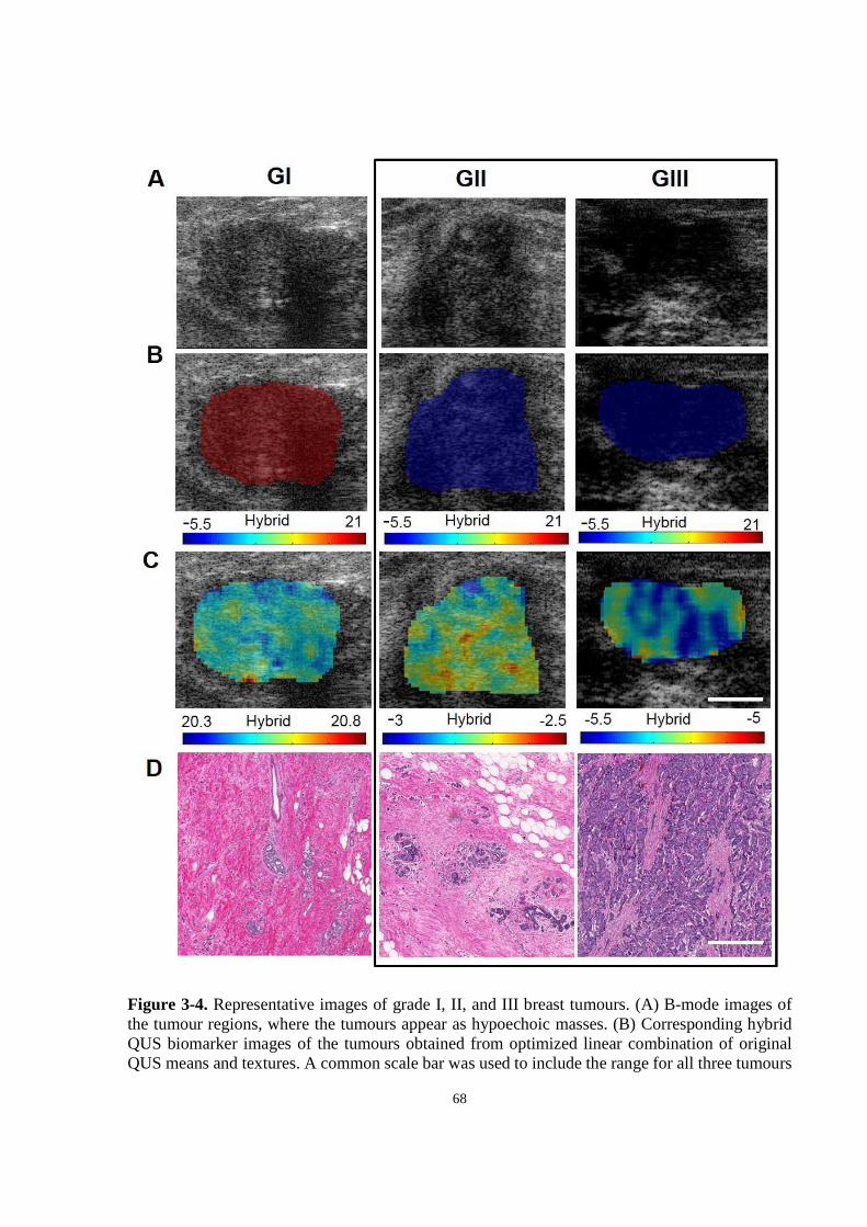
68

Figure 3-4. Representative images of grade I, II, and III breast tumours. (A) B-mode images of the tumour regions, where the tumours appear as hypoechoic masses. (B) Corresponding hybrid QUS biomarker images of the tumours obtained from optimized linear combination of original QUS means and textures. A common scale bar was used to include the range for all three tumours

69

(C) Same images as (B) but with the use of individual scale bars to show the tumour heterogeneity (D) Hematoxylin and eosin stained histopathology images of the tumours. Scale bars: 1 cm (US), 100 µm (hist).

3.5 Discussion

In summary, multiparametric analysis of advanced scattering parameters extracted from the RF

ultrasound signal backscattered from breast tumours can sensitively (88%) and specifically (91%)

distinguish tumours from proximal normal breast tissue. While the mean values of QUS parametric

maps were all poor in differentiating tumour grades, textural analysis techniques on QUS

parametric maps better discriminated between grade I and grade II-III breast tumours. After

acquiring several planes of RF data from tumours of patients with LABC, features such as mean,

CON, COR, ENE, and HOM were extracted from QUS parametric maps computed from tumour

ROIs within the breast. An optimal feature set was selected using sequential feature selection and

linear discriminant analysis was performed on the set with cross-validation, using true labels

identified histopathologically from biopsy specimens. Three types of feature sets were considered:

feature selection from means, textures, and the combinations of means and textures. The most

accurate classification was obtained when the combination of QUS means and textures were used

(86% accuracy).

Quantitative ultrasound has been investigated in the past as an aid to characterize breast tumours

in vivo and to differentiate malignant breast tumours from benign masses [21], [42], [66], [70].

Specifically, the work of Oelze et al. [21] has demonstrated the ability to differentiate mouse

mammary carcinoma from benign rat fibroadenomas using mean values of scatterer size and

acoustic concentration parametric maps obtained from a 20 MHz ultrasound system. On the other

hand here, the differentiation between lower grade tumours (analogous to benign fibroadenomas)

and mid-to-high grade tumours (analogous to mammary carcinoma) was best seen using the

textural features of AAC and ASD, giving accuracy as high as 86%. Mean values yielded less than

optimal separation (79 %). Similarly, when Nasief et al. [70] investigated QUS parameters such

as scatterer size, attenuation, and heterogeneity index to differentiate clinically benign breast

tumours from malignant ones, only subtle differences could be found, since only mean values were

considered. The parametric images here (Figure 3-4. Representative images of grade I, II, and III

breast tumours. (A) B-mode images of the tumour regions, where the tumours appear as

70

hypoechoic masses. (B) Corresponding hybrid QUS biomarker images of the tumours obtained

from optimized linear combination of original QUS means and textures. A common scale bar was

used to include the range for all three tumours (C) Same images as (B) but with the use of

individual scale bars to show the tumour heterogeneity (D) Hematoxylin and eosin stained

histopathology images of the tumours. Scale bars: 1 cm (US), 100 µm (hist).

), however, suggested clear distinctions between tumours of different grades when textures of QUS

parameters were included.

In the tumour versus normal tissue study, the difference in the classification performance obtained

using SAS, AAC and SAS, AAC, ASD was not assessed in a statistical sense. The 1% increase in

accuracy may not be statistically significant. In the future, on could perform bootstrapping in order

to obtain a number of classification accuracies for each feature set, and perform a significance test

between the two-feature QUS and three-feature QUS models. Nevertheless, the obtained

accuracies with the two-feature and three-feature QUS models were sufficiently high to warrant

clinical application of our method as an aid for radiologists in tumour identification in breast

ultrasound images.

Previous studies on the application of textural analysis techniques for ultrasound-based breast

tissue characterization have been limited to those aimed to differentiate predominantly between

benign and malignant masses using plain B-mode images [66]. Such studies have in the past raised

concerns regarding reproducibility, mainly due to instrument dependency and lack of parameter

normalization [65], [66]. Consequently, the results obtained in those studies could vary from one

imaging system to another, since the GLCMs were computed from B-mode images. Here, a GLCM

computed from a quantitative ultrasound parametric map obtained from normalized power spectra

(which are phantom-calibrated) would be in principle instrument independent. In this study, texture

analysis of the QUS parametric maps of different grades of breast tumours demonstrated a strong

separation when the combination of texture features (CON, COR, ENE, HOM) of the parametric

maps were used (82% accuracy). A further improvement in classification was achieved when the

means of parametric maps were combined with the textures (86% accuracy).

It is acknowledged that relatively lower G1 prediction rates were obtained compared to GII-III

prediction rates. This is likely due to the presence of imbalanced data, where there are many more

71

grade II-III cases than grade I cases, producing a bias in the classification results. Compensation

for imbalanced datasets is an active area of research and requires thorough investigation in a

separate study. Nevertheless a leave-one-out analysis here was able to fairly accurately identify

grade I tumours compared to grade II-III tumours which are often managed differently in terms of

clinical care.

As previously mentioned, acoustic concentration is the product of scatterer number density and

acoustic impedance difference between the scatterer and the background, and acoustic impedance

is the product of sound speed and density. Thus, the fact that parameters related to the scatterer

spacing and acoustic concentration including SAS, AAC, MBF, and SI formed the major portion

of the disrciminant function (Table 3-4) compared to parameters related to the scatterer size (i.e.

SS and ASD) suggests that the spatial organization and material properties of the tumour

microstructure play a more important role than its size in the discrimination of tumour histological

grades. This was not surprising since the breast tumour is a complex tissue containing blood

vessels, adipose tissue, and stroma, in addition to cancerous glands. Thus, scatterer size may not

refer to the size of glands alone, but to a mixture of structures. The results here stimulate

investigation into a better scattering model, for example, one which accounts for dense packing of

cells in tumours. The structure factor model has been suggested recently as a scattering model

which provides theoretical solution for the BSC accounting for high scatterer concentrations

reflected in tumour tissues [71]. The search of a better attenuation estimation algorithm (i.e. one

that accounts for tissue heterogeneity) is also warranted.

In summary, breast tumour grading is an important part of breast cancer diagnosis and provides

valuable information for treatment planning. In this light, non-invasive methods such as texture-

based QUS analysis can provide beneficial diagnostic information which can be applied before

and during the course of treatment. This study demonstrated a high potential for textural

characteristics of QUS parametric maps to be used in the diagnosis and grading of breast tumours.

The best tissue classification could be achieved when the combination of mean and textural

properties of MBF, SS, SI, SAS, ASD, and AAC parametric maps were used. This work provides

a framework for future clinical studies in which the proposed classification scheme is evaluated

on larger cohorts of patients in order to further assess its capabilities for an accurate breast tumour

diagnosis and grading, non-invasively.

72

4 Quantitative ultrasound assessment of breast tumour response to chemotherapy

73

4.1 Overview

Purpose: This study demonstrated the ability of quantitative ultrasound parameters in providing

an early prediction of tumour response to neoadjuvant chemotherapy in patients with locally

advanced breast cancer.

Methods: Ultrasound data consisting of raw RF data were collected from 58 locally advanced

breast cancer patients prior to chemotherapy treatment and at 4 times during their treatment (weeks

0, 1, 4, 8, and prior to surgery) using 6-MHz ultrasound. Quantitative ultrasound parameters

including linear regression spectral parameters (midband fit, spectral slope, 0-MHz intercept),

scatterer spacing, attenuation coefficient estimate, and backscatter coefficient parameters (average

scatterer diameter and average acoustic concentration) were determined. Ultrasound data were

compared with the ultimate clinical and pathological response of the patient's tumour to treatment

and patient recurrence-free survival.

Results: Midband fit, 0-MHz intercept, and attenuation coefficient estimate parameters increased

statistically significantly in patients with treatment-responding tumours compared to

nonresponding patients as early as 1 week after the start of the treatment. In contrast, tumour size

change was not found to be significantly different in responders and non-responders. Discriminant

analysis using the K nearest neighbour classifier demonstrated that the best classification

performance could be achieved using the combination of midband fit, spectral slope, and scatterer

spacing, with an accuracy of 60 ± 10 % at week 1, 77 ± 8 % at week 4 and 75 ± 6 % at week 8.

Furthermore, when the QUS measurements at each time (week) were combined with pre-treatment

(week 0) QUS information, the classification accuracies improved (70 ± 9 % at week 1, 80 ± 5 %

at week 4, and 81 ± 6 % at week 8). Finally, the QUS classification model demonstrated a

significant difference in survival rates of responding and nonresponding patients at weeks 1 and 4

(p=0.035, and 0.027, respectively).

Conclusion: This study demonstrates for the first time, using new parameters tested on a relatively

large patient cohort and leave-one-out classifier evaluation, that a hybrid QUS biomarker including

attenuation-corrected midband fit, spectral slope, and scatterer spacing, can detect the response of

LABC tumours to neoadjuvant chemotherapy with 80% accuracy as early as after 4 weeks. The

findings of this study also incorporated novel pre-treatment ultrasonic scattering properties of a

tumour improving results. This work demonstrates the potential of quantitative ultrasound and

74

machine learning methods for predicting the response of breast tumours to chemotherapy early

and guiding personalized medicine with regards to the treatment planning of refractory patients.

4.2 Introduction

Conventional methods of clinical tumour response assessment involve tracking changes in tumour

size, using the guidelines provided by RECIST [6]. Such measurements are ascertained using

anatomical-based imaging modalities such as X-ray imaging, magnetic resonance imaging (MRI),

or conventional diagnostic ultrasound. However, these size-based metrics typically provide late

indications of response as measurable changes in tumour size do not occur until several weeks to

months after the initiation of the chemotherapy treatment, despite positive response [7]. Currently

no routine clinical imaging is carried out to assess tumour size or response during breast

chemotherapy administration in a neoadjuvant setting. This study determined the ability of

quantitative ultrasound parameters extracted from raw (radiofrequency) tumour-based ultrasound

data in predicting patient-based tumour responses early in the course of neoadjuvant

chemotherapy.

Tumour shrinkage is known to be the late cumulative effect of cell death induced by anti-cancer

therapy. Previous studies which have used early biomarkers obtained from tumour biopsy samples

have demonstrated that increased tumour apoptosis occurring early in the course of therapy was

associated with good clinical response, and consequently an improved patient survival [8]. Thus,

the introduction of a non-invasive functional imaging biomarker that can be used to monitor the

early response of a tumour to anticancer therapy can potentially help facilitate personalized

treatment for cancer patients.

Ultrasound, commonly used clinically for screening, diagnosis, and image-guided procedures, due

to its low cost, quick imaging time, high resolution, and ionizing radiation-free nature, has recently

been explored by investigators as a potential imaging modality for tumour response monitoring

[28]. This was achieved in that study using QUS, which used a quantitative analysis of the

frequency content of the RF signals backscattered from breast tumours in patients undergoing

chemotherapy. According to the theoretical formulation of ultrasound scattering, the tissue power

spectrum is affected by parameters such as the size and number density of the constituent

75

scatterers. Thus, based on inherent differences in the microstructures of different tissues,

parameters obtained from the tissue power spectrum, including MBF, SI, and SS, have enabled the

characterization of abnormalities of different tissues such as those in breast, prostate, liver, eye,

myocardium, and lymph nodes [14], [16], [18]–[20], [22], [24]. These parameters of interest are

estimated from a linear regression analysis of the tissue power spectrum within the usable

bandwidth (usually corresponding to −6 dB range), representing the slope (SS) and intercept (SI)

of the line, as well as the value of the line at the center of the frequency bandwidth (MBF).

Alternatively, some studies have found higher-order model derived parameters such ASD and

AAC to be useful in studying tissues, including differentiating mouse models of breast cancer from

benign breast masses, grading clinical breast cancer, and detecting cancerous human lymph nodes

[16], [21], [24]. In regards to applications in treatment monitoring, Sadeghi-Naini et al. [28]

posited that at a clinically relevant frequency range (<10 MHz), spectral parameters such as MBF,

SI, and SS are sensitive to changes in tumour microstructure which occur as a result therapeutic

effects, and therefore can correlate to early signatures of tumour response. Using linear

discriminant analysis, they demonstrated that the combination of MBF and SI parameters provided

100% sensitivity and 83% specificity in the detection of response of tumours to chemotherapy.

More recently, Tadayyon et al. [72] demonstrated that estimating the acoustic attenuation of the

patient's tumour and correcting the power spectra accordingly, not previously done [28], increased

the sensitivity of MBF to response detection by 12% and specificity by 17%. Moreover, the

performance measures reported by Sadeghi-Naini et al. were obtained without cross-validation

and due to the small sample size (N = 25), clinical feasibility was limited. Here, I propose a new

approach for QUS prediction of breast tumour response to neoadjuvant chemotherapy tested on a

relatively large database of breast US data (N = 58), incorporating attenuation estimation and

correction of the power spectra. The study here performed discriminant analysis using a more

advanced classifier - k nearest neighbour (KNN) classifier. The KNN classification was performed

using leave-one-patient-out cross-validation, not performed in previous studies. In addition to

classical spectral parameters (MBF, SS, and SI) previously investigated, I have also investigated

the utility of advanced BSC parameters (ASD and AAC), SAS, as well as ACE in predicting the

therapeutic response of breast tumours.

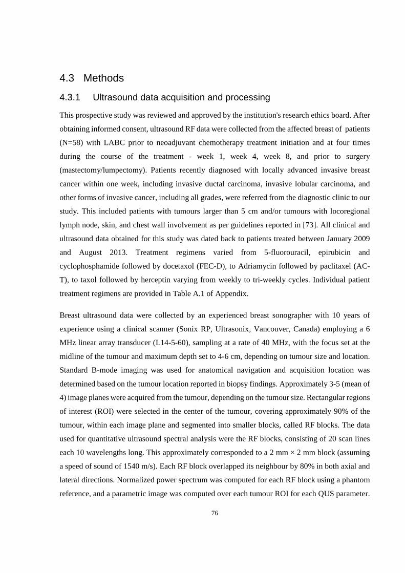
76

4.3 Methods

4.3.1 Ultrasound data acquisition and processing

This prospective study was reviewed and approved by the institution's research ethics board. After

obtaining informed consent, ultrasound RF data were collected from the affected breast of patients

(N=58) with LABC prior to neoadjuvant chemotherapy treatment initiation and at four times

during the course of the treatment - week 1, week 4, week 8, and prior to surgery

(mastectomy/lumpectomy). Patients recently diagnosed with locally advanced invasive breast

cancer within one week, including invasive ductal carcinoma, invasive lobular carcinoma, and

other forms of invasive cancer, including all grades, were referred from the diagnostic clinic to our

study. This included patients with tumours larger than 5 cm and/or tumours with locoregional

lymph node, skin, and chest wall involvement as per guidelines reported in [73]. All clinical and

ultrasound data obtained for this study was dated back to patients treated between January 2009

and August 2013. Treatment regimens varied from 5-fluorouracil, epirubicin and

cyclophosphamide followed by docetaxol (FEC-D), to Adriamycin followed by paclitaxel (AC-

T), to taxol followed by herceptin varying from weekly to tri-weekly cycles. Individual patient

treatment regimens are provided in Table A.1 of Appendix.

Breast ultrasound data were collected by an experienced breast sonographer with 10 years of

experience using a clinical scanner (Sonix RP, Ultrasonix, Vancouver, Canada) employing a 6

MHz linear array transducer (L14-5-60), sampling at a rate of 40 MHz, with the focus set at the

midline of the tumour and maximum depth set to 4-6 cm, depending on tumour size and location.

Standard B-mode imaging was used for anatomical navigation and acquisition location was

determined based on the tumour location reported in biopsy findings. Approximately 3-5 (mean of

4) image planes were acquired from the tumour, depending on the tumour size. Rectangular regions

of interest (ROI) were selected in the center of the tumour, covering approximately 90% of the

tumour, within each image plane and segmented into smaller blocks, called RF blocks. The data

used for quantitative ultrasound spectral analysis were the RF blocks, consisting of 20 scan lines

each 10 wavelengths long. This approximately corresponded to a 2 mm × 2 mm block (assuming

a speed of sound of 1540 m/s). Each RF block overlapped its neighbour by 80% in both axial and

lateral directions. Normalized power spectrum was computed for each RF block using a phantom

reference, and a parametric image was computed over each tumour ROI for each QUS parameter.

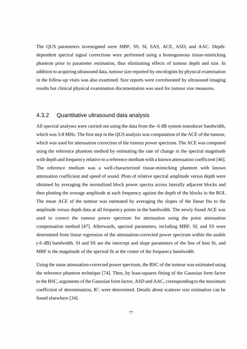
77

The QUS parameters investigated were MBF, SS, SI, SAS, ACE, ASD, and AAC. Depth-

dependent spectral signal corrections were performed using a homogeneous tissue-mimicking

phantom prior to parameter estimation, thus eliminating effects of tumour depth and size. In

addition to acquiring ultrasound data, tumour size reported by oncologists by physical examination

in the follow-up visits was also examined. Size reports were corroborated by ultrasound imaging

results but clinical physical examination documentation was used for tumour size measures.

4.3.2 Quantitative ultrasound data analysis

All spectral analyses were carried out using the data from the -6 dB system transducer bandwidth,

which was 3-8 MHz. The first step in the QUS analysis was computation of the ACE of the tumour,

which was used for attenuation correction of the tumour power spectrum. The ACE was computed

using the reference phantom method by estimating the rate of change in the spectral magnitude

with depth and frequency relative to a reference medium with a known attenuation coefficient [46].

The reference medium was a well-characterized tissue-mimicking phantom with known

attenuation coefficient and speed of sound. Plots of relative spectral amplitude versus depth were

obtained by averaging the normalized block power spectra across laterally adjacent blocks and

then plotting the average amplitude at each frequency against the depth of the blocks in the ROI.

The mean ACE of the tumour was estimated by averaging the slopes of the linear fits to the

amplitude versus depth data at all frequency points in the bandwidth. The newly found ACE was

used to correct the tumour power spectrum for attenuation using the point attenuation

compensation method [47]. Afterwards, spectral parameters, including MBF, SI, and SS were

determined from linear regression of the attenuation-corrected power spectrum within the usable

(-6 dB) bandwidth. SI and SS are the intercept and slope parameters of the line of best fit, and

MBF is the magnitude of the spectral fit at the center of the frequency bandwidth.

Using the same attenuation-corrected power spectrum, the BSC of the tumour was estimated using

the reference phantom technique [74]. Then, by least-squares fitting of the Gaussian form factor

to the BSC, arguments of the Gaussian form factor, ASD and AAC, corresponding to the maximum

coefficient of determination, R2, were determined. Details about scatterer size estimation can be

found elsewhere [34].

78

Whereas spectral linear regression and BSC models are based on incoherent scattering, cepstral

analysis techniques permit coherent scattering properties of tissues to be derived and coherent

structures to be identified [75]. For cepstral analysis, the power spectrum of the tumour was

determined by modeling the tumour echo signal as an autoregressive signal and using Burg's

algorithm to estimate its power spectrum [76]. The power spectrum was then normalized to that of

a planar reflector. By computing the autocorrelation of the normalized power spectrum, the SAS

parameter was determined from the frequency at which the peak occurred in the autocorrelation.

The implementation of this technique followed the technique used by Tadayyon et al. to estimate

SAS in breast tumours and normal tissues, which demonstrated a separation between breast

tumours of different histological grades [24].

After computing all 7 QUS features for all patients, discriminant analysis was performed using the

KNN classifier and using all possible combinations of QUS features. The KNN classifier

determines the class of a point in the feature space based on the class which forms the majority of

the points neighbouring the point of interest and based on the distance between those points and

the point of interest [77].

4.3.3 Classification and statistical analyses

All QUS results were compared with the clinical standard response of each patient, determined

based on the RECIST guideline. This was determined at the end of the their several-month

treatment by measuring the reduction in gross tumour size based on dynamic contrast enhanced

magnetic resonance images (DCE-MRI) cross-verified with whole-mount breast histopathology

obtained post-operatively. Since the focus of this study was a binary classification of response, the

standard four categories of response defined in the RECIST guideline were merged into two

categories by grouping complete and partial responses into “response” and grouping stable and

progressive disease responses into “nonresponse”. A recent study demonstrated that residual

tumour cellularity is an important prognostic factor in breast cancer neoadjuvant treatment, which

should be taken into account in conjunction with the RECIST metric of bulk tumour shrinkage

(BTS) [78]. Accordingly in this study, a patient was deemed to be a clinical responder if the sum

of the lengths of the tumour foci was reduced by more than 30% or if in the non-mass enhancing

79

area, the pathologically determined residual tumour cellularity was low. A patient was deemed to

be a clinical non-responder if the sum of the lengths of their tumour foci was reduced by less than

30% or the residual tumour cellularity remained high.

The mean changes in each QUS parameter were compared between the clinical responder and non-

responder groups at each time. Initially, a Shapiro-Wilk normality test was used to test each

parametric data set for normality. Since all data sets passed the normality test, a student's unpaired

t-test (right-tailed, α=0.05) was used to test for statistical significance of the difference between

group means. In order to determine the clinical feasibility of using QUS as a cancer therapy

monitoring system, multi-feature response classification was performed using the KNN algorithm

based on Euclidean distances. Rather than the absolute values, the changes in the QUS parameters

relative to their pre-treatment value (week 0) were used as classification features, which are

denoted here by the prefix ∆ (i.e. ∆MBF). This baseline normalization was necessary in order to

minimize inter-patient variability of each parameter. The imbalance in the data set was

compensated for by randomly sampling (with replacement) from the responder group so as to have

equal number of responders and non-responders (N=16). All patients in the non-responder group

were used for training and testing the classifier (N=16). Classification was performed 10 times (10

different responder group samples) with leave-one-patient-out evaluation. Since the number of

QUS features was small (n=7), an exhaustive search method was used for obtaining the optimal

subset of features. During the exhaustive search a leave-one-patient-out cross-validation was

performed to obtain classification results. This accounted for the classifier’s generalization ability

and inter-subject variability, as suggested in the literature [79]. The accuracy was used as the

objective function to maximize. The metrics used for measuring classification performance were

sensitivity, specificity, and accuracy.

4.4 Results

Patient characteristics, including age, initial tumour size, tumour subtypes, and bulk tumour

shrinkage for responders and non-responders are summarized in Table 4-1. All patients were

females aged between 29 and 67 years with a mean age of 50 years. Tumour size ranged from 2 to

13 cm, with a mean size of 6.3 cm. The tumours were mainly of the invasive ductal carcinoma

80

type not otherwise specified (90% of cases). The remaining 10% of cases were comprised of

invasive lobular carcinoma (5%) and other types of breast cancer (5%). The ultimate clinical

response rate to chemotherapy in the sample population was 72% and responders demonstrated a

tumour shrinkage of 68 ± 47% whereas the non-responders demonstrated mean bulk shrinkage of

-16 ± 57%. Bulk tumour shrinkage was defined as the relative reduction in the sum of tumour

diameters from pre-treatment to pre-operation. Size measurements were ascertained using breast

DCE-MRI obtained at these two times. Detailed individual patient characteristics and responses

are provided in Tables A.1 and A.2 of Appendix.

Representative images of a responding breast tumour and a nonresponding breast tumour before

treatment start and 4 weeks after treatment start (1-2 cycles of chemotherapy) are presented in

Figure 4-1 and Figure 4-2. For each tumour, B-mode images, MBF images overlaid on the B-

modes, power spectra before and 4 weeks after the start of treatment, and magnified hematoxylin

and eosin (H&E) stained histology sections of whole-mount breast specimens obtained post-

surgery (mastectomy/lumpectomy) are shown. These data were selected for illustration as MBF

was a parameter which demonstrated statistically significant changes at early weeks (1 and 4).

Whereas B-mode images showed no appreciable changes in the tumour 4 weeks into treatment, a

marked increase in MBF could be observed in the responding tumour region as a result of 4 weeks

of chemotherapy treatment (1-2 cycles). The nonresponding tumour, on the other hand,

demonstrated no change or decrease in MBF. The before/after superimposed power spectra

demonstrate the same concept graphically, where MBF is marked by a circle in the middle of the

regression line (Figure 4-1 and Figure 4-2, C left). There is a small offset between the MBF values

in the MBF images and MBF values in the power spectra. This is due to the fact that the shown

power spectrum plots were obtained by averaging the power spectra from all RF blocks within the

ROI, whereas the MBF values in the MBF images were obtained from representative individual

power spectra of individual RF blocks within the ROI. The histology image of the responding

tumour indicates a stroma-filled tissue (pink staining) with small isolated patches of glands (purple

staining), demonstrating therapeutic effects. On the other hand, the histology of the nonresponding

tumour shows a gland-dominated tumour with low stromal collagen density, indicating little to no

therapeutic effect.

81

Figure 4-3 compares QUS parameters and the RECIST-based tumour size reduction for tracking

changes in the tumour during chemotherapy. Average QUS data obtained from responding and

nonresponding groups are plotted versus treatment time in Figure 4-3A-G. Patients were grouped

based on their ultimate clinical/pathological responses. The vertical axes represent changes in QUS

parameters relative to week 0 (pre-treatment). Parameters related to the intensity of the frequency-

dependent backscatter (i.e. ∆MBF, ∆SI, ∆AAC) demonstrated, on average, an increase with

treatment time for responders. Based on unpaired t-test comparison of responder and non-

responder groups, two-tailed with 95 % confidence, this increase was statistically significant at

weeks 1, 4, and 8 for ∆MBF (p = 0.042, <0.005, <0.005, respectively), and at weeks 1, 4, and 8

for ∆SI (p = 0.034, 0.010, <0.005, respectively). Patients in the responding group demonstrated a

greater increase in ∆ACE compared to non-responders, which were statistically significant at

weeks 1 and 4 (p <0.005 and 0.042, respectively). On the other hand, ∆SS, ∆ASD, and ∆SAS

values did not show any significant changes between responders and non-responders at any time

during the treatment. As expected, the mean tumour size reduction shown in Figure 4-3H was not

significantly different in responders versus non-responders at any time (p = 0.89, 53, and 0.42 at

week 1, 4, and 8, respectively) except at the end of the several-month treatment (p = 0.0011 at pre-

op). Whereas a 30% mean size reduction occurred in responders at week 4 (Figure 4-3H), non-

responders also had a mean reduction of almost 30% at week 4, and the difference between the

groups was not statistically significant. After week 4, whereas responding tumours continued

shrinking, nonresponding tumours regrew to 20 % larger than their original size between week 8

and pre-op, which had approximately an 8 to 10 week gap.

In order to compare the effectiveness of different QUS parameters in differentiating responding

tumours from nonresponding ones, the KNN algorithm was run for each QUS parameter separately

and classification accuracy was computed. Table 4-2 summarizes the performance of individual

QUS parameters in predicting response in terms of classification accuracy and statistical

significance (p-value) for weeks 1, 4, and 8. The classification results are based on a 2-neighbour

search area and using the Euclidian distance metric, which provided the optimal classification. The

results demonstrated that the MBF parameter was most effective in response detection at all weeks

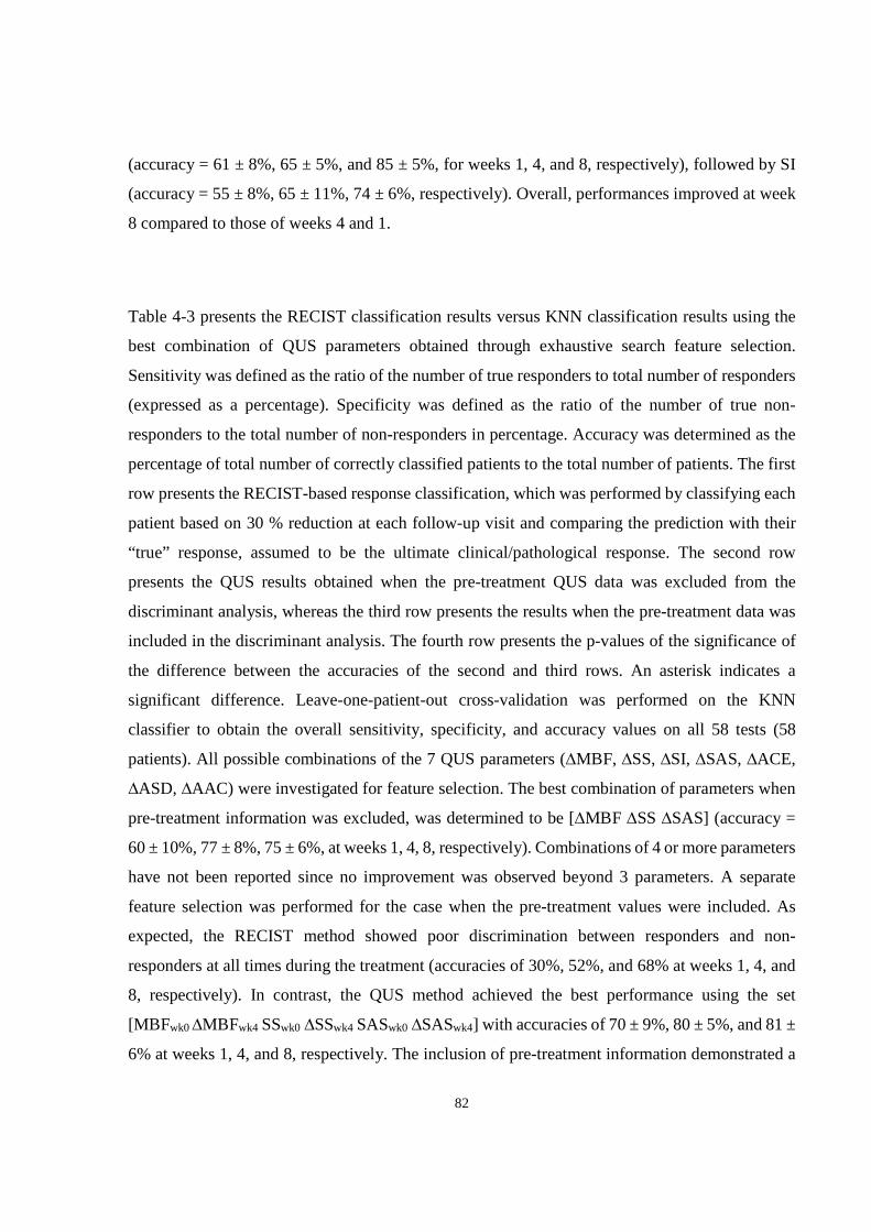
82

(accuracy = 61 ± 8%, 65 ± 5%, and 85 ± 5%, for weeks 1, 4, and 8, respectively), followed by SI

(accuracy = 55 ± 8%, 65 ± 11%, 74 ± 6%, respectively). Overall, performances improved at week

8 compared to those of weeks 4 and 1.

Table 4-3 presents the RECIST classification results versus KNN classification results using the

best combination of QUS parameters obtained through exhaustive search feature selection.

Sensitivity was defined as the ratio of the number of true responders to total number of responders

(expressed as a percentage). Specificity was defined as the ratio of the number of true non-

responders to the total number of non-responders in percentage. Accuracy was determined as the

percentage of total number of correctly classified patients to the total number of patients. The first

row presents the RECIST-based response classification, which was performed by classifying each

patient based on 30 % reduction at each follow-up visit and comparing the prediction with their

“true” response, assumed to be the ultimate clinical/pathological response. The second row

presents the QUS results obtained when the pre-treatment QUS data was excluded from the

discriminant analysis, whereas the third row presents the results when the pre-treatment data was

included in the discriminant analysis. The fourth row presents the p-values of the significance of

the difference between the accuracies of the second and third rows. An asterisk indicates a

significant difference. Leave-one-patient-out cross-validation was performed on the KNN

classifier to obtain the overall sensitivity, specificity, and accuracy values on all 58 tests (58

patients). All possible combinations of the 7 QUS parameters (∆MBF, ∆SS, ∆SI, ∆SAS, ∆ACE,

∆ASD, ∆AAC) were investigated for feature selection. The best combination of parameters when

pre-treatment information was excluded, was determined to be [∆MBF ∆SS ∆SAS] (accuracy =

60 ± 10%, 77 ± 8%, 75 ± 6%, at weeks 1, 4, 8, respectively). Combinations of 4 or more parameters

have not been reported since no improvement was observed beyond 3 parameters. A separate

feature selection was performed for the case when the pre-treatment values were included. As

expected, the RECIST method showed poor discrimination between responders and non-

responders at all times during the treatment (accuracies of 30%, 52%, and 68% at weeks 1, 4, and

8, respectively). In contrast, the QUS method achieved the best performance using the set

[MBFwk0 ∆MBFwk4 SSwk0 ∆SSwk4 SASwk0 ∆SASwk4] with accuracies of 70 ± 9%, 80 ± 5%, and 81 ±

6% at weeks 1, 4, and 8, respectively. The inclusion of pre-treatment information demonstrated a

83

statistically significant up to 10 % improvement in the accuracies at weeks 1 and 8 (p-value = 0.03,

0.04, respectively).

In order to compare the predictions of QUS and histopathology on the recurrence free survival

(RFS) of the patients, Kaplan-Meier survival analysis was performed and the results are presented

in Figure 4-4. The median follow-up time was 25 months. The RFS curves were divided into

responder and non-responder groups. A log-rank test was performed to compare the RFS rates

between the responders and non-responders using the method described in [80]. The RFS curves

obtained from QUS biomarkers demonstrated statistically significant differences between the

response groups at weeks 1 and 4 (log-rank p-value = 0.035, 0.027, respectively) as did the RFS

curves obtained from histopathology information (log-rank p-value = 0.0002). However, RFS

curves obtained from QUS biomarkers at week 8 did not show significant difference between the

response groups (log-rank p-value = 0.26).

84

Table 4-1. Summary of patient characteristics. IDC = invasive ductal carcinoma, ILC = Invasive

lobular carcinoma, BTS = bulk tumour shrinkage (percent change in tumour size).

Characteristic Total (N=58) No. %

Age (y) 49 ± 10 Tumour subtype

IDC 52 90 ILC 3 5 Other 3 5

Responders 42 72 BTS (%) 68 ± 47

Non-responders 16 28 BTS (%) -16 ± 57

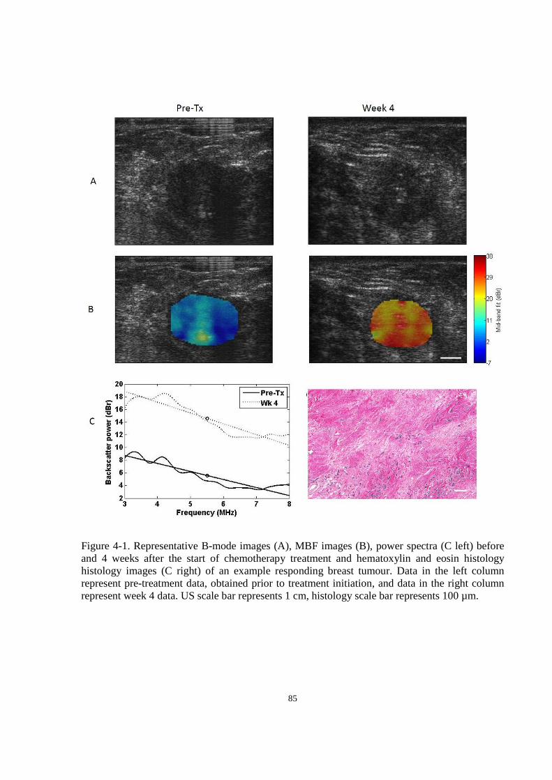
85

Figure 4-1. Representative B-mode images (A), MBF images (B), power spectra (C left) before and 4 weeks after the start of chemotherapy treatment and hematoxylin and eosin histology histology images (C right) of an example responding breast tumour. Data in the left column represent pre-treatment data, obtained prior to treatment initiation, and data in the right column represent week 4 data. US scale bar represents 1 cm, histology scale bar represents 100 µm.

86

Figure 4-2. Representative B-mode images (A), MBF images (B), power spectra (C left) before and 4 weeks after the start of chemotherapy treatment and hematoxylin and eosin histology histology images (C right) of an example nonresponding breast tumour. Data in the left column represent pre-treatment data, obtained prior to treatment initiation, and data in the right column represent week 4 data. US scale bar represents 1 cm, histology scale bar represents 100 µm.

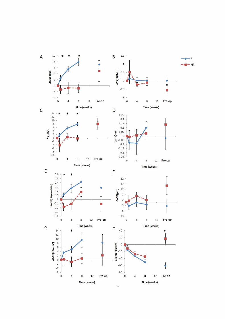
87

88

Figure 4-3. Comparison between QUS parameters (A-G) and the RECIST-based tumour size reduction (H) for tracking patient tumours during chemotherapy. QUS and RECIST values were averaged over responder (blue diamond) and non-responder (red square) groups, and plotted over the treatment time. Patients were grouped based on their pathological clinical response determined post-chemotherapy. All values were normalized to week 0 by subtraction. Error bars represent standard error of the mean.

Table 4-2. A comparison of the classification performances (accuracy) of different QUS parameters using the KNN classifier, at weeks 1, 4 and 8. The bold entry indicates the best performance. Reported values are mean and standard deviation of the accuracies obtained by running the classification 10 times using 10 random samples of responders.

Week 1 Accuracy Week 4 Accuracy Week 8 Accuracy ∆MBF 61 ± 8 65 ± 5 85 ± 5 ∆SS 53 ± 8 62 ± 7 63 ± 15 ∆SI 55 ± 8 65 ± 11 74 ± 6 ∆ACE 54 ± 8 64 ± 4 60 ± 10 ∆SAS 62 ± 7 58 ± 8 69 ± 7 ∆ASD 54 ± 9 61 ± 9 60 ± 13 ∆AAC 58 ± 8 64 ± 9 69 ± 8

Table 4-3. A comparison of the classification results obtained based on tumour size alone (RECIST criteria), based on changes in QUS parameters, and based on changes in QUS parameters plus week 0 QUS parameters. ∆QUS represents [∆MBF ∆SS ∆SAS] and QUSw0 represents [MBFw0 SSw0 SASw0]. The last row presents the p-value significance of the difference between the mean accuracies of ∆QUS and ∆QUS + QUSw0 models. Reported values are mean and standard deviation of the accuracies obtained by running the classification 10 times using 10 bootstrap samples from responder group. For QUS results, sensitivity and specificity numbers have denominator of 16 and accuracy numbers have denominator of 32.

Week 1 Week 4 Week 8

Sens Spec Acc Sens Spec Acc Sens Spec Acc

RECIST No. 5/32 9/15 14/47 19/36 6/12 25/48 26/33 4/11 30/44

% 16 60 30 53 50 52 79 36 68

∆QUS No. 10 ± 2 9 ± 1 19 ± 3 13 ± 2 12 ± 2 25 ± 3 12 ± 1 12 ± 1 24 ± 2

% 61 ± 13 59 ± 9 60 ± 10 79 ± 10 76 ± 11 77 ± 8 78 ± 8 72 ± 9 75 ± 6

∆QUS + QUSw0

No. 12 ± 2 10 ± 2 11 ± 1 13 ± 1 13 ± 1 26 ± 2 12 ± 1 13 ± 1 26 ± 2

% 76 ± 11 64 ± 11 70 ± 9 80 ± 9 79 ± 5 80 ± 5 78 ± 9 83 ± 7 81 ± 6

p-value 0.03* 0.33 0.04*

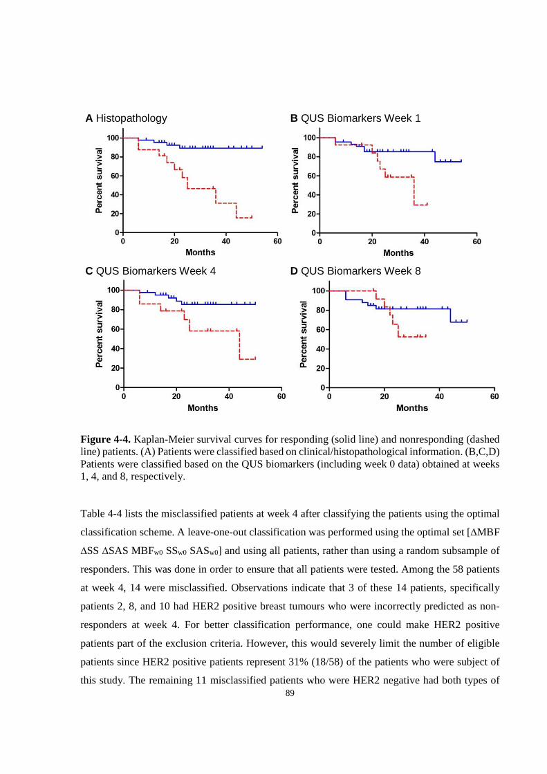
89

Figure 4-4. Kaplan-Meier survival curves for responding (solid line) and nonresponding (dashed line) patients. (A) Patients were classified based on clinical/histopathological information. (B,C,D) Patients were classified based on the QUS biomarkers (including week 0 data) obtained at weeks 1, 4, and 8, respectively. Table 4-4 lists the misclassified patients at week 4 after classifying the patients using the optimal

classification scheme. A leave-one-out classification was performed using the optimal set [∆MBF

∆SS ∆SAS MBFw0 SSw0 SASw0] and using all patients, rather than using a random subsample of

responders. This was done in order to ensure that all patients were tested. Among the 58 patients

at week 4, 14 were misclassified. Observations indicate that 3 of these 14 patients, specifically

patients 2, 8, and 10 had HER2 positive breast tumours who were incorrectly predicted as non-

responders at week 4. For better classification performance, one could make HER2 positive

patients part of the exclusion criteria. However, this would severely limit the number of eligible

patients since HER2 positive patients represent 31% (18/58) of the patients who were subject of

this study. The remaining 11 misclassified patients who were HER2 negative had both types of

A Histopathology B QUS Biomarkers Week 1

C QUS Biomarkers Week 4 D QUS Biomarkers Week 8

90

misclassifications (responder and non-responder). Again, making HER2 negative patients (69%)

part of the exclusion criteria would severely limit the number of eligible patients. No other pattern

was observed about the misclassified patients. A larger cohort of patients should be analyzed (100+

patients) in order to better understand the outliers.

Table 4-4. Clinical/histopathological characteristics of misclassified patients at week 4. The majority were HER2 negative patients (indicated in bold), and the few HER2 positive patients (indicated in italics) all received HER2 receptor-targeted treatments such as Herceptin and Trastuzumab.

Pt No.

Initial Tumour dimensions

(AP x ML x SI) Histology Grade ER PR HER2 Treatment Predicted

Response

1 13 x 11 IDC III - - - AC + paclitaxel NR

2 6x7x3 IMC NA + + + AC +

paclitaxel + Herceptin

NR

3 3x3.5x1.5 IDC III - - - FEC-D NR

4 4.9 x 4.9 x 4.1 IDC III + + - AC +

docetaxel NR

5 5.2 x 4 x 4 IDC II + + - FEC +

docetaxel NR

6 8 x 10 IDC II + + - Dose-dense

AC + paclitaxel

R

7 4.4 x 3.9 x 5.8 IDC II + + - AC + paclitaxel R

8 2.4 x 2.7 x 3.2 IDC II - - + AC +

paclitaxel, trastuzumab

NR

9 6.4 x 3.2 x 8.7 ILC II + + - FEC-D R

10 5.4 x 5 x 8 IDC II + + +

AC + docetaxel, paclitaxel,

trastuzumab

NR

11 3.3 x 3.4 x 3.4 IDC III - - - TC NR

12 2.7 x 3.2 x 2.0 IDC III + + - ACT R

13 2.3 x 2.5 x 2.5 & 1.0 x 1.0 x

0.7 IDC III - - -

AC + paclitaxel R

14 10 x 5 x 10.5 IDC III - - - dose dense AC + taxol

NR

91

4.5 Discussion

This study demonstrated, for the first time, using a relatively large patient database and using a

leave-one-patient out classifier evaluation, that multi-parametric quantitative ultrasound applied at

a clinically relevant frequency range (<10 MHz) can be used to non-invasively predict breast

tumour response to chemotherapy as early as after 1-2 cycles (1-4 weeks) with reasonable accuracy

(80%), long before a tumour size change provided discriminative information (many months later

(pre-op)). Additionally, RFS analyses performed demonstrated that when the ultrasound

biomarkers [MBF, SS, SAS], which include pre-treatment values along with the change at a

specified time during treatment, were used to predict the RFS, responder and non-responder RFS

rates were statistically significantly different when classifying patients based on data at weeks 1

and 4. Although the results of this study were not used to modify the treatments of the patients, the

findings suggest that ultrasound biomarkers can predict the RFS rates of responding and

nonresponding patients within weeks almost as accurately as patient ultimate clinical response

based on clinical and histopathology information obtained many months later. The reason for the

poor separation of the RFS rates of the groups predicted from week 8 QUS data was likely due to

initial responses to chemotherapy challenge inherently being more predictive but could be

influenced due to the relatively small sample size or other physiological changes.

Previously developed theories about ultrasound detection of cell death support the findings in this

study, where just as the parameters related to the backscatter intensity and acoustic concentration

(i.e. MBF and SI) increased in tumours undergoing cell death in vivo [27], MBF, SI, and AAC

values increased in clinically responding tumours in this study. Classification analysis determined

that MBF was the most effective parameter in the classification at weeks 4 and 8 (Table 4-2). This

is likely due to the fact that MBF is affected by frequency-dependent attenuation whereas SI and

AAC are not (they are affected by depth-dependent attenuation). Since changes in ACE obtained

at weeks 1 and 4 were statistically significant in responders compared to those of non-responders

(p = 0.004 and 0.039, respectively), it is likely that the attenuation correction of the tumour spectra

helped in accentuating the MBF parameter to response detection. Furthermore, the MBF changes

in the responding-tumour patient population became highly statistically different from those of

nonresponding tumours at week 8 (p < 0.005). The increase in the ACE observed in responding

tumours over treatment time was concordant with the increase in attenuation coefficient with cell

death extent observed in previous high-frequency QUS cell treatment characterization studies [62].

92

Classification analysis demonstrated that increasing the number of QUS parameters submitted to

the classification scheme improved the classification, but not beyond three parameters. Whereas

previous studies found classical parameters (MBF and SI) to be sensitive to detecting breast tumour

response at 4 weeks, I found that MBF, SI, ACE, and AAC all have comparable accuracies in

predicting tumour response (65 %, 65 %, 64 %, and 64 % respectively at week 4). Combining the

changes and pre-treatment values of MBF, SS, and SAS provided the best prediction of response

(70 ± 9% at week 1, 80 ± 5% at week 4, and 81 ± 6 and week 8). This may be due to structural

tumour properties before chemotherapy being linked to tumour aggressiveness and consequently

the likelihood of not responding to chemotherapy.

Other imaging methods have been used in research to assess the therapeutic responses of locally

advanced breast tumours, including diffuse optical spectroscopy (DOS) [12], positron emission

tomography (PET) [7], and dynamic contrast-enhanced magnetic resonance imaging (DCE-MRI)

[7]. Despite a favorable sensitivity in detecting breast tumour response at 4 weeks, DOS has limited

tissue penetration depth without complex reconstruction methods, thereby limiting its application

to superficial tumours. DCE-MRI remains expensive and requires a contrast agent which can be

toxic to patients with kidney diseases and PET requires the injection of radioactive tracer isotopes,

limiting repeated usability and imparting potential long term health complications. On the other

hand, ultrasound is relatively inexpensive and safe and its imaging methods with respect to

quantitative ultrasound rely on the inherent changes in tissue microstructure to generate tissue

contrast, requiring no external contrast agents. Recently, a genetic method of monitoring metastatic

breast cancer has been proposed, demonstrating circulating tumour DNA as an effective biomarker

for this purpose [81]. However, the method is invasive in its nature, and DNA quantification and

genetic sequencing are costly and time consuming. The method here does not rely on tumour

specific genetic markers but is sensitive to the biophysical changes which accompany cell death –

the induction of which is the goal of cancer chemotherapy. Evidence demonstrates that patients

who respond well to chemotherapy may benefit from longer regimens of efficacious chemotherapy

and suggest that ineffective treatments should be changed [82].

93

Limitations

Currently the standard of care for patients receiving neoadjuvant chemotherapy only includes pre-

treatment and post-treatment imaging, using typically DCE-MRI, but does not routinely include

intra-treatment imaging for tumour size assessment. Furthermore, ultrasound imaging is not

reliable for tumour size measurement due to attenuation artefacts which cast shadows on the distal

end of deep-set tumours. However, this had minimal effect on QUS assessment, since the ROIs

were selected in the center of the tumour (~ 90 % coverage), avoiding regions of artefacts.

Although tumour size was recorded in this study as measured by the physician during follow-up

physical examinations, this method has limited reproducibility since measurements were made by

different physicians. Thus, measurements reported here should be assumed approximate.

A point of note is that within the six optimal parameters which were found for treatment response

discrimination, ∆MBF (week 0 and 4) parameter was the most accurate single classifying

parameter, but ∆SS (week 0 and 4) and ∆SAS (week 0 and 4), were less accurate than other

parameters investigated, according to data in Table 4-2. However, since each of these parameters

describe independent features of the underlying tissue microstructure, the discriminating power

increased when these parameters were combined. Particularly, MBF describes the acoustic

concentration, SS describes the size of the scatterers, and SAS describes the distance between

regularly-spaced scatterers. Although the large number of selected features (six) compared to the

number of observations (N=58) may raise concerns of overfitting, the leave-one-patient-out

analysis performed on the data has been known to minimize overfitting [83].

The QUS results obtained indicated poor separation between responders and non-responders at the

pre-operative scan time. This is expected and likely due to the large time gap between the end of

neoadjuvant treatment and surgery (usually several weeks), where minimal or no cell death had

occurred at the time of data acquisition. Additionally, tumour ROI selection in pre-operative

images was difficult in complete pathologic responders who had no residual tumour, and were

therefore excluded from the analysis. As expected the early investigated times at weeks 1 and 4

indicated the best separation between responders and non-responders. These were selected to span

cycles of chemotherapy and it remains unknown if other times sooner or later would be useful for

analyses. Despite this the sensitivity and specificity and consequent accuracy were significant for

predicting ultimate patient clinical response.

94

Conclusions

In summary, this study demonstrated for the first time, using a relatively large patient cohort and

leave-one-out classifier evaluation, that the hybrid QUS biomarker [∆MBF, ∆SS, ∆SAS] can, with

good sensitivity and specificity, detect the response of LABC tumours to neoadjuvant

chemotherapy as early as after 1 cycle (1 week) of administration. Extending efficacious treatments

and switching ineffective ones early based on indications of QUS biomarkers may likely result in

improved RFS. The findings of this study also provided insight into pre-treatment ultrasonic

scattering properties of a tumour potentially contributing to a prediction about its therapeutic

resistance before the initiation of therapy.

95

5 Summary and future directions

96

5.1 Summary and conclusions of thesis

Breast cancer is the most common cancer among Canadian women [1] and its heterogeneity of

response necessitates personalization of therapy [73]. Although neoadjuvant chemotherapy prior

to surgery is the clinically favourable option for patients with locally advanced breast cancer,

different patients respond differently to the same chemotherapy and currently, the response is not

known until completion of a therapy spanning several months. Various chemical- and image-based

biomarkers have been developed to probe early changes in tumour function/metabolism.

Biochemical methods include analysis of aoptotic index, Ki-67, and Bcl-2 from tumour biopsy

samples. Image-based methods include DW-MRI, FDG-PET, and DOI imaging. This thesis

evaluated—for the first time—the capacity of ultrasound (particularly quantitative ultrasound) in

detecting early changes in tumour microstructure related to cell death response to chemotherapy

in a clinical setting. Ultrasound has a number of advantages including relatively low cost, short

imaging time, high resolution, radiation-free nature, and intrinsic tumour contrast which does not

require injection of any contrast agents.

Chapter 2 demonstrated in vivo that certain ultrasonic scattering properties estimated from

backscatter coefficients are linearly correlated to the cell death fraction (CDF). Whereas previous

studies had demonstrated a correlation between linear regression spectral parameters (i.e. MBF

and SI) and CDF at the clinically relevant frequency range [27], this thesis demonstrated, in the

same frequency range, that normalizing advanced QUS parameters such as AAC to initial tumour

volume will result in improved correlation to CDF (r2 for ∆AAC was 0.399, for ∆AACVN was

0.639). This suggests that QUS parameters are affected by initial tumour volume, which is

associated with the presence and prevalence of hypoxic and/or necrotic cores within the tumour

(larger tumours often have hypoxic, necrotic cores). The findings of this study provided a

framework for QUS analysis in the subsequent clinical studies in Chapters 3 and 4. Specifically,

the scattering model to use for estimating ASD and AAC was determined (the spherical Gaussian

model), and the CDF related to QUS changes was evaluated early (4 to 48 hours) from

chemotherapy onset, in order to mimic the changes expected in clinical breast tumours within a

few days of initiating a course of chemotherapy.

In Chapter 3, the QUS characteristics of clinical breast tumours versus normal breast tissue and

different grades of breast tumours were investigated. The true labels were obtained from biopsy

97

information. It was demonstrated that the combination of AAC and SAS can be used to

differentiate breast tumours from surrounding breast tissue with 88% using a quadratic

discriminant function. Furthermore, grade I breast tumours could be differentiated from grade II-

III tumours using the combination of means and textures of QUS parametric images of MBF, SS,

SI, SAS, ACE, ASD, and AAC with an accuracy of 86%. The accuracy was based on leave-one-

patient-out cross-validated classification results. In a clinical setting, the incorporation of QUS

assessment of the breast during or after an ultrasound-guided breast biopsy session potentially may

permit cross-verification of the histological findings.

In Chapter 4, the QUS characteristics of LABC patients undergoing neoadjuvant chemotherapy

were investigated using a multiparameter approach employing machine learning methods. Patients

were classified as responders or nonresponders, where the true response was based on

clinical/histopathological information obtained at the end of the treatment. Employing the k-

nearest neighbour classifier and leave-one-patient-out evaluation, it was determined that the

combination of MBF, SS, and SAS can be used to differentiate responders and nonresponders with

accuracies of 60 ± 10%, 77 ± 8%, and 75 ± 6% at weeks 1, 4, and 8 respectively. Furthermore,

when pre-treatment QUS measurements were included in the classification, the accuracies

improved (70 ± 9%, 80 ± 5%, and 81 ± 6%, at weeks 1, 4, and 8 respectively). Tumour biomarker

studies have demonstrated that increased tumour apoptosis is associated with positive response,

which is associated with improved patient survival. Thus, the clinical implication of this finding is

that patients undergoing neoadjuvant chemotherapy of LABC can potentially benefit from a

weekly QUS assessment in order to evaluate the early response of the tumour and alter the regimen

if the tumour was nonresponsive.

There are, however, limitations to the proposed method which clinicians should be aware of. First,

the method is not 100% sensitive nor 100% specific at classifying responding patients versus

nonresponding patients. It was shown in Chapter 4 that patients with HER2-negative breast cancers

and those receiving HER2-targeted treatments may not benefit from this approach as our

investigated QUS parameters are not sensitive nor specific to this type of cancer or treatment type.

Investigation is underway to discover new QUS features that may be more sensitive and specific

to response prediction. Some potentially effective approaches are GLCM-based texture analysis

which were demonstrated in chapter 3 to be effective in characterizing LABC tumour subtypes

when combined with mean QUS features. Additionally, increasing the number of patients in such

98

a study may permit the classifier to better learn the data and result in higher sensitivity and

specificity. If performance does not improve, our QUS methods may be used in conjunction with

other methods such as DW-MRI, PET, and/or DOS to potentially improve the response detection

performance compared to using any one method alone.

Another limitation of our proposed technique is that the definition of true response is based on

bulk tumour shrinkage post-treatment as well as residual tumour cellularity. However, accurate

measurement of tumour shrinkage requires accurate delineation of tumour boundaries, which

becomes especially difficult as the tumour undergoes morphological changes in response to

treatment. Additionally, tumour cellularity (high or low) can be subjective depending on the

pathologist examining the specimen. Researchers are developing more accurate and functional

response markers such as Ki-67 and AI, which have been demonstrated as predictive of both

response and disease-free survival [8][9]. Thus, a better understanding of the relation between our

measured QUS features and the tumour’s biological changes may be gained if correlation analyses

were performed between QUS features and these biomarkers.

5.2 Future directions

The idea of extending QUS-based response monitoring to other cancer sites is promising. One

potential site would be the prostate. The standard of care for patients with hormone refractory

prostate cancer is chemotherapy, due to its demonstrated prolonged survival [84]. However, no

imaging method for monitoring the response of these patients to chemotherapy is available in the

clinical setting, although molecular analysis based on circulating tumour cells has been proposed

as a potential method [85]. Quantitative ultrasound imaging has demonstrated superior capability

in delineating prostate cancers compared to conventional B-mode images, for guidance of prostate

biopsies and treatments [86]. Thus, there is promise that similar QUS techniques can also be used

to track changes in the prostate tumour during chemotherapy.

One of the challenges in this thesis was the lack of three-dimensional ultrasound data. Three-

dimensional (3D) imaging is important in medicine for visualizing the extent of disease and its

surrounding anatomy. Availability of 3D ultrasound data from the whole breast would facilitate

identification and tracking of the tumour from one scan session to another, especially when

substantial changes in tumour morphology occur during treatment. 3D reconstruction from

99

freehand ultrasound scanners is difficult due to the irregular spacing and orientation of the image

planes. Reconstruction algorithms have been proposed with limited success [87]. An alternative

solution is the use of 3D ultrasound imaging systems, such as ultrasound computed tomography

(Figure 5-1) and rotating concave transducer technologies (Figure 5-2).

The issue of variability in ROI selection arose on multiple occasions during the manuscript review

processes. Since tumour ROIs were selected manually, the user variation of the ROI selection

results in variations in QUS features and difficult reproducibility. An automated breast tumour

segmentation process might alleviate such issues. Numerous algorithms have been proposed, such

as local texture analysis and clustering approaches [88], [89]. Such approaches have demonstrated

high sensitivity and specificity in terms of similarity to the radiologist's manual delineations (92%

sensitivity and 93% specificity for the clustering approach, 95% sensitivity and 92% specificity

for the local texture approach). However, these methods were tested on high-contrast tumours in

ultrasound images. Some breast tumours have low ultrasound contrast, for which segmentation

results were not reported in those studies, and will likely fail. Perhaps the optimal choice would be

to have a semiautomated tumour ROI selection, where the low-contrast tumours are selected

manually.

In regards to the ground truth determinations of patient responses, a limitation exists: the ground

truth is based on preoperative MRI and histopathological findings on the postsurgical breast

specimen. These data are obtained at the end of the several-month neoadjuvant treatment whose

effectiveness is under assessment. No ground truth is available at times concordant with QUS

assessment (i.e. weeks 1, 4, and 8). One way to address this issue and improve the experimental

design is to use existing molecular biomarkers such as apoptotic index (AI) and proliferation (Ki-

67) as reference measures of response, as suggested in one study [8]. One can measure Ki-67 by

immunocytochemical analysis and AI by flow cytometric analysis of fine needle aspiration biopsy

samples obtained coincident with the QUS imaging sessions. This can help identity the biological

changes occurring in the tumour to which QUS parameters are sensitive. If the changes in QUS

parameters were correlated with AI, then the expectation that QUS changes are correlated with

therapy-induced tumour cell death in the human breast will be confirmed.

The quantitative ultrasound treatment monitoring technique used in this thesis has recently

received interest from the health care and research communities and fundraising is underway to

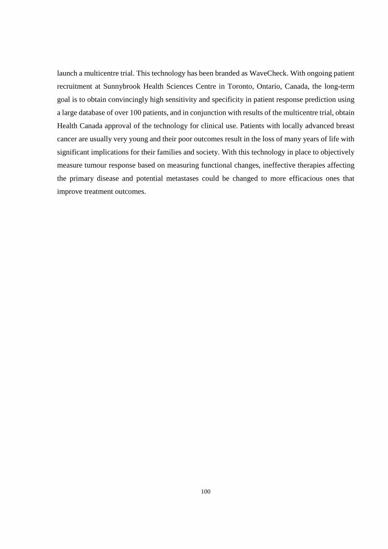
100

launch a multicentre trial. This technology has been branded as WaveCheck. With ongoing patient

recruitment at Sunnybrook Health Sciences Centre in Toronto, Ontario, Canada, the long-term

goal is to obtain convincingly high sensitivity and specificity in patient response prediction using

a large database of over 100 patients, and in conjunction with results of the multicentre trial, obtain

Health Canada approval of the technology for clinical use. Patients with locally advanced breast

cancer are usually very young and their poor outcomes result in the loss of many years of life with

significant implications for their families and society. With this technology in place to objectively

measure tumour response based on measuring functional changes, ineffective therapies affecting

the primary disease and potential metastases could be changed to more efficacious ones that

improve treatment outcomes.

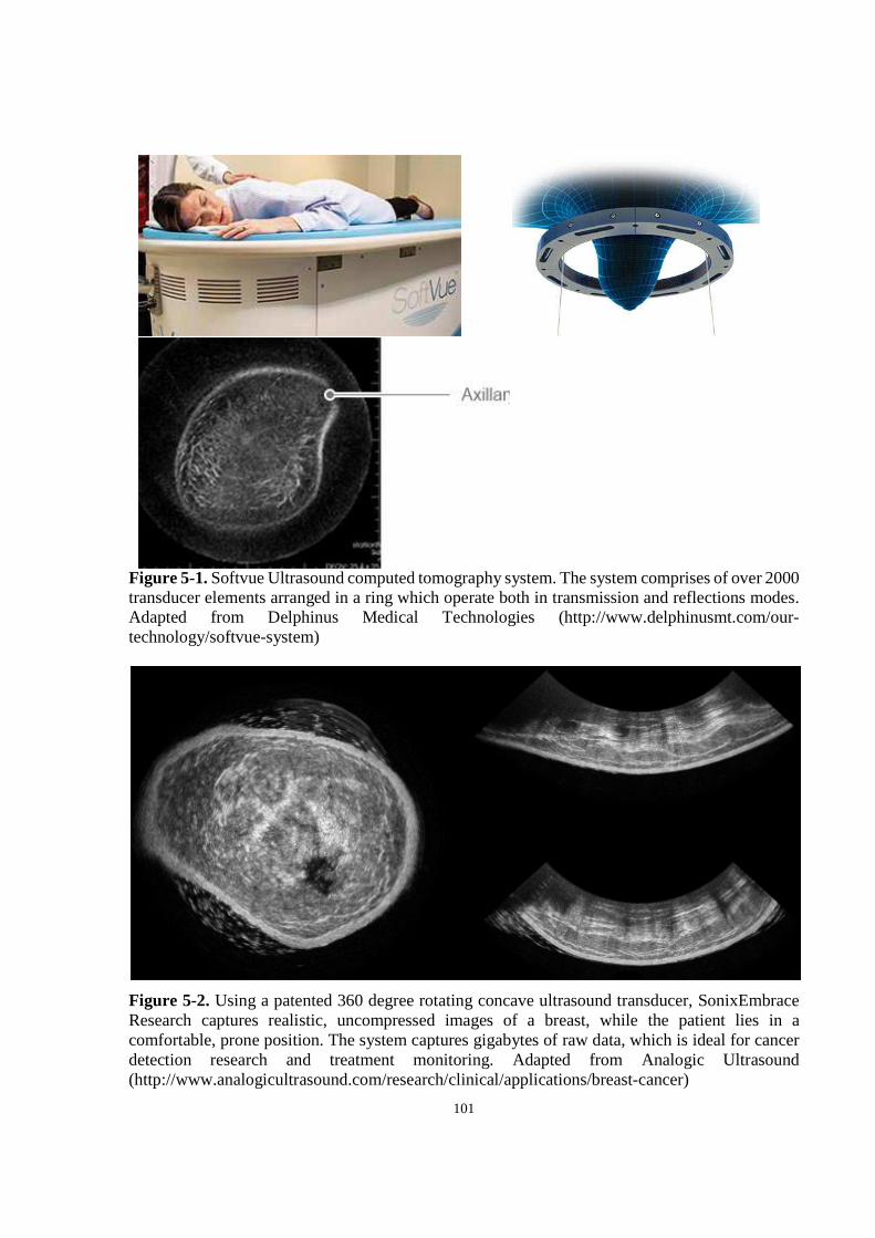
101

Figure 5-1. Softvue Ultrasound computed tomography system. The system comprises of over 2000 transducer elements arranged in a ring which operate both in transmission and reflections modes. Adapted from Delphinus Medical Technologies (http://www.delphinusmt.com/our-technology/softvue-system)

Figure 5-2. Using a patented 360 degree rotating concave ultrasound transducer, SonixEmbrace Research captures realistic, uncompressed images of a breast, while the patient lies in a comfortable, prone position. The system captures gigabytes of raw data, which is ideal for cancer detection research and treatment monitoring. Adapted from Analogic Ultrasound (http://www.analogicultrasound.com/research/clinical/applications/breast-cancer)

102

Appendix

103

Analytical solution for the scattering from solid spheres

James Faran derived the equation of the scattered pressure by a solid sphere of radius � in a

fluid-like medium that is insonified by a plane harmonic wave, ©] = © e�«¬­5���®. With the

assumption of distant observation point (g ≫ �), the solution was obtained by spherical wave

decomposition, yielding,

where �� is the wave number defined as ����­ , where �is the speed of sound in the medium

surrounding the scatterer, r is the observation point, n is the order number, ° is the angle of

incidence, ©X is the Legendre polynomial, and ±X is defined by,

±X = tan�� tan�UX(\�)� Mtan(²X) + tan(7X(\�))OMtan(²X) + tan(³X(\�))O A2

UX = tan��M− }X(\�)%X(\�)O A3

7X = tan�� ´− \}Xµ (\�)}X(\�) ¶ A4

³X = tan�� ´− \%Xµ (\�)%X(\�) ¶ A5

²X = tan��M−·�·� N�%¸X(\�, #)O A6

ξº(x�, σ) = tan��−x��2 ½ \�}Xµ (\�)\�}Xµ (\�) − }X(\�) − 2(%� + %)}X(\�)(%� + % − 2)}X(\�) + \��}X′′(\�)¿\�� À σ1 − 2σ }X(\�) − }Xµµ(\�)Á\�}Xµ (\�) − }X(\�) − 2(%� + %)M}X(\�) − \�}Xµ (\�)O(%� + % − 2)}X(\�) + \��}Xµµ(\�)

A7

|©����, g| ≈ © ��g Ã>�2% + 1 sin�±X �WÆy©X uÇ°ÈXG à for g ≫ � A1

104

\� = ���

\� = ���

\� = ���

A8

where σ is the Poisson’s ratio of the scatterer, }Xand %X are the spherical Bessel functions of the

first and second kind, respectively, the primes denote derivatives, � is the scatterer radius, �� is

the wavenumber calculated from the compressional wave speed in the scatterer, and �� is the

wavenumber calculated from the shear wave speed in the scatterer. Note that equation A7

includes Hickling’s correction [90] where the factor É

���É is placed inside the brackets rather

than outside. Using the definition of the backscatter coefficient,

A9

where R is the distance to the scattering volume, and V is the scattering volume. Knowing the

number of scatterers per unit volume, %&, average scattered intensity, < IË0>, and incident

intensity, Iͺ0, A10

A11

2sc

bscinc

IR

V Iσ =

2

02sc

sc

pI nV

cρ=

20

02inc

PI

cρ=

105

One can obtain an expression of the backscatter coefficient of a solid spherical scattering sample

as,

#$ = %&�� Ã>(2% + 1) sin(±X) �WÆy©X uÇ°È

XG �

A12

106

Patient characteristics

Table A-1. Patient characteristics and administered chemotherapy regimens

Pt No.

Age Initial tumour

Dimensions (AP x ML x SI)

Histology Grade ER PR HER2 Treatment

1 55 5.4 x 5 x 2.3 cm IDC I - + + FEC and Taxol,

Herceptin

2 53 7.4 x 7 cm IDC with

mucineous features

I + + - Epi and Taxotere

3 41 5.3 x 4.4 x 4.7

cm IDC II + + +

Docetaxel, carboplatin, trastuzumab

4 65 RB 10x10cm IDC I - - - AC & Taxotere

5 50 NA IDC III + + + AC +

docetaxel, trastuzumab

6 33 3x3cm IDC I + + - AC & Taxol

7 33 5.4 x 5 x 8 IDC II + + +

AC + docetaxel, paclitaxel,

trastuzumab 8 48 4.9 x 4.9 x 4.1 IDC III + + - AC + docetaxel 9 36 4.4 x 3.9 x 5.8 IDC II + + - AC + paclitaxel

10 40 4.4 x 3.4 IDC III - - - AC + paclitaxel

11 62 12 x 14 IDC II-III - - - FEC +

docetaxel 12 59 6 x 2.3 x 4.3 IDC III - - - AC + paclitaxel

13 53 8.4 x 9.4 x 12.7 Metaplastic carcinoma

III - - -

AC + cisplatinum, gemcitabine

platinum

14 48 7 x 9 cm IDC II + + + AC-Taxol and

Herceptin 15 50 13 x 11 IDC III - - - AC + paclitaxel

16 49 7.1 x 5.5 x 8.9 IDC III - - + Docetaxel,

trastuzumab

17 40 3 x 2.4 x 3 IDC III + + + AC +

paclitaxel, trastuzumab

18 56 2.4 x 2.7 x 3.2 IDC II - - + AC +

paclitaxel, trastuzumab

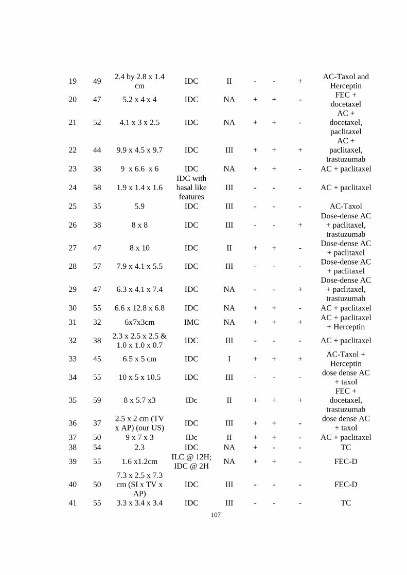
107

19 49 2.4 by 2.8 x 1.4

cm IDC II - - +

AC-Taxol and Herceptin

20 47 5.2 x 4 x 4 IDC NA + + - FEC +

docetaxel

21 52 4.1 x 3 x 2.5 IDC NA + + - AC +

docetaxel, paclitaxel

22 44 9.9 x 4.5 x 9.7 IDC III + + + AC +

paclitaxel, trastuzumab

23 38 9 x 6.6 x 6 IDC NA + + - AC + paclitaxel

24 58 1.9 x 1.4 x 1.6 IDC with basal like features

III - - - AC + paclitaxel

25 35 5.9 IDC III - - - AC-Taxol

26 38 8 x 8 IDC III - - + Dose-dense AC

+ paclitaxel, trastuzumab

27 47 8 x 10 IDC II + + - Dose-dense AC

+ paclitaxel

28 57 7.9 x 4.1 x 5.5 IDC III - - - Dose-dense AC

+ paclitaxel

29 47 6.3 x 4.1 x 7.4 IDC NA - - + Dose-dense AC

+ paclitaxel, trastuzumab

30 55 6.6 x 12.8 x 6.8 IDC NA + + - AC + paclitaxel

31 32 6x7x3cm IMC NA + + + AC + paclitaxel

+ Herceptin

32 38 2.3 x 2.5 x 2.5 & 1.0 x 1.0 x 0.7

IDC III - - - AC + paclitaxel

33 45 6.5 x 5 cm IDC I + + + AC-Taxol + Herceptin

34 55 10 x 5 x 10.5 IDC III - - - dose dense AC

+ taxol

35 59 8 x 5.7 x3 IDc II + + + FEC +

docetaxel, trastuzumab

36 37 2.5 x 2 cm (TV x AP) (our US)

IDC III + + - dose dense AC

+ taxol 37 50 9 x 7 x 3 IDc II + + - AC + paclitaxel 38 54 2.3 IDC NA + - - TC

39 55 1.6 x1.2cm ILC @ 12H; IDC @ 2H

NA + + - FEC-D

40 50 7.3 x 2.5 x 7.3 cm (SI x TV x

AP) IDC III - - - FEC-D

41 55 3.3 x 3.4 x 3.4 IDC III - - - TC

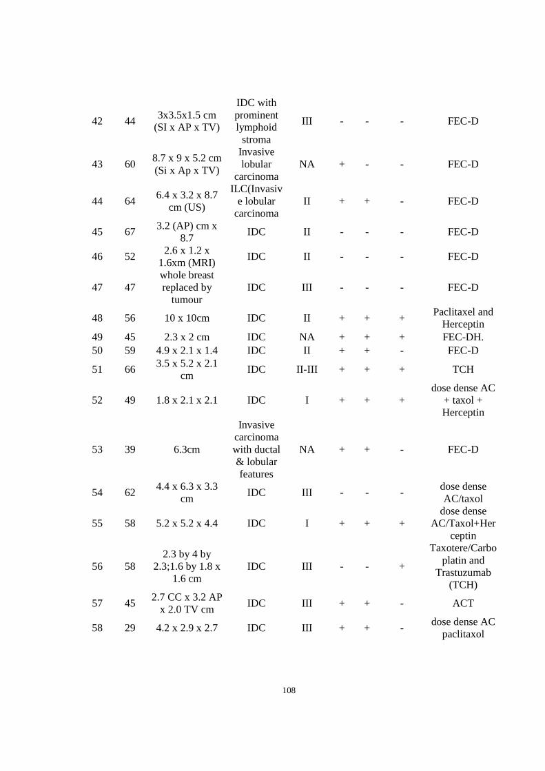
108

42 44 3x3.5x1.5 cm

(SI x AP x TV)

IDC with prominent lymphoid stroma

III - - - FEC-D

43 60 8.7 x 9 x 5.2 cm (Si x Ap x TV)

Invasive lobular

carcinoma NA + - - FEC-D

44 64 6.4 x 3.2 x 8.7

cm (US)

ILC(Invasive lobular

carcinoma II + + - FEC-D

45 67 3.2 (AP) cm x

8.7 IDC II - - - FEC-D

46 52 2.6 x 1.2 x

1.6xm (MRI) IDC II - - - FEC-D

47 47 whole breast replaced by

tumour IDC III - - - FEC-D

48 56 10 x 10cm IDC II + + + Paclitaxel and

Herceptin 49 45 2.3 x 2 cm IDC NA + + + FEC-DH. 50 59 4.9 x 2.1 x 1.4 IDC II + + - FEC-D

51 66 3.5 x 5.2 x 2.1

cm IDC II-III + + + TCH

52 49 1.8 x 2.1 x 2.1 IDC I + + + dose dense AC

+ taxol + Herceptin

53 39 6.3cm

Invasive carcinoma with ductal & lobular features

NA + + - FEC-D

54 62 4.4 x 6.3 x 3.3

cm IDC III - - -

dose dense AC/taxol

55 58 5.2 x 5.2 x 4.4 IDC I + + + dose dense

AC/Taxol+Herceptin

56 58 2.3 by 4 by

2.3;1.6 by 1.8 x 1.6 cm

IDC III - - +

Taxotere/Carboplatin and

Trastuzumab (TCH)

57 45 2.7 CC x 3.2 AP

x 2.0 TV cm IDC III + + - ACT

58 29 4.2 x 2.9 x 2.7 IDC III + + - dose dense AC

paclitaxol

109

Table A-2. Response of patients to administered regimens

Pt no. Residual tumour

size DCIS Extent Notes Response

1 no residual absent Complete pathological response good

2 7 x 5 x 3 cm absent Carcinoma with mucinous features; Very low cellularity good

3 2.7 x 2.5 x 2.4 5 to 10 Tumour cellularity remains very high poor

4 1.6 x 0.8 x 0.5 cm <5 good 5 No residual absent Complete pathological response good 6 1.4cm NA Good response good 7 no residual NA Complete pathological response good

8 1.4 x 1 x 1 20 Small volume of invasive tumour remaining good

9 11.4 <5 Extensive residual disease poor

10 no residual NA

Complete pathological response, with only fibrous tumour bed remaining good

11 No residual NA Complete pathological response good

12 2.6 x 2.5 x 2.5 absent Good response good

13 whole breast NA Residual tumour took up all the breast; no response poor

14 5cm NA she did not respond to first drug poor 15 4cm absent Good response good

16 no residual 100 (2 x 1.5 x 1cm)

Complete pathological response, with only in situ disease remaining good

17 no residual 100%(0.2 x 0.2 cm)

Complete pathological response, with only in situ disease remaining good

18 0.2 x 0.2 absent Very good response good 19 1.4 x 2.4 x 1.4 cm 90 0.1 cm good

20 6.5 5 to 10

Invasive carcinoma grows in single cells and nest of few cells. Although the overall size of invasive carcinoma is 6.5 cm, the cellularity is exceedingly low thus the overall volume of the tumour is also very low. Probable or definite response good

21 no residual 100%(1x0.7x0.6cm)

Complete pathological response, with only in situ disease remaining good

110

22 2 x 1 x 1 & 1.6 x 1 x

0.5 80 Good response, tumour cellularity is low good

23 2.9 x 2 x 1.5 & 2 x

1.5 x 1 60 Tumour cellularity is low good

24 0.15 100%(1.5mm)

Complete pathological response, with only fibrous tumour bed remaining good

25 no residual absent complete response good 26 No residual absent Complete pathological response good 27 12.5 x 4.5 x 3.5 <5 No definite response poor

28 no residual absent

No residual invasive carcinoma in the breast, only lymphovascular invasion remaining good

29 scattered (small

amnt)

Complete pathological response, only scattered in-situ component remaining good

30 17 <5% No definite response poor

31 7.4cm 5 to 10

bed of sscattered microscopic cancer foci; tumour focus is 0.6cm good

32

2.8(3.8) x 3.02.2) x 2.3(2.2) & 1.5 x 1.6

x 1.1 <5% No definite response poor

33 2.8 + 2 cm 30 multiple foci of invasive carcinoma poor

34 2foci (0.3+0.5mm) absent good 35 No residual absent no residual good

36 2.2 x 1.5 x 1.1 cm,

single focus <5 poor

37 1.2 14.54545455 Small volume of invasive tumour remaining good

38 5.5 6.666666667 scattered clusters good

39 1.2 x 0.9 x 0.7 cm <5 multiple foci of invasive carcinoma poor

40 2.1cm 60 cellularity 20%; scattered small clusters of tumour cells good

41 1.8 cm absent Single focus of invasive carcinoma; no def rep good

42 no residual carcinoma absent good

43

2 foci of invasive carcinoma; 8.0 x 5.0 x 4.5 cm and 3.0 x

2.5 x 1.7 cm absent poor 44 19cm absent poor

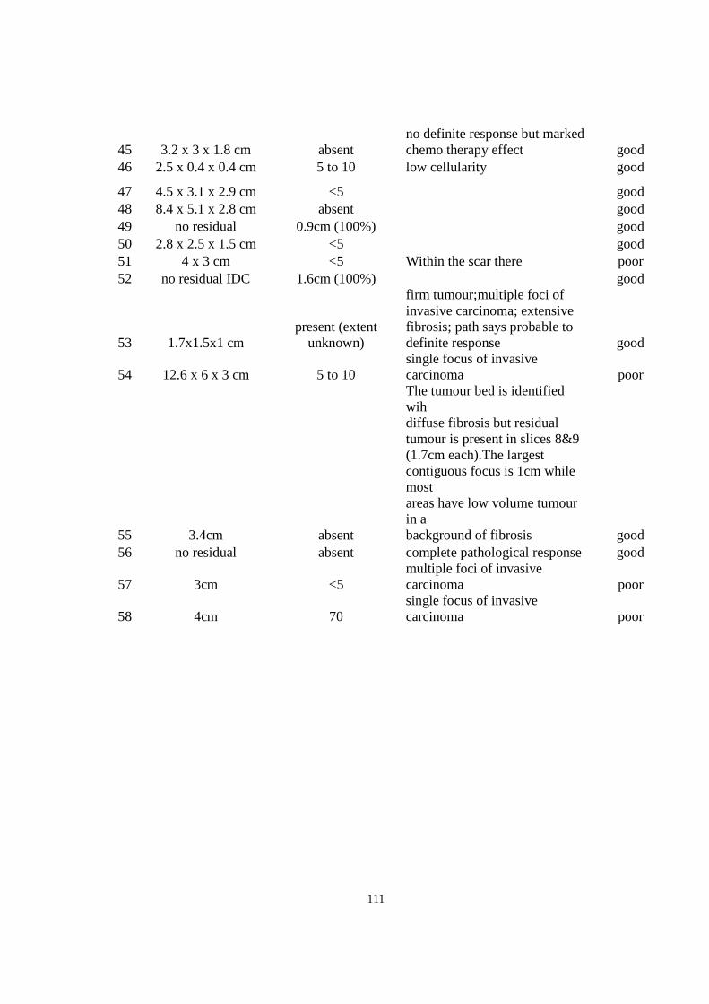
111

45 3.2 x 3 x 1.8 cm absent no definite response but marked chemo therapy effect good

46 2.5 x 0.4 x 0.4 cm 5 to 10 low cellularity good

47 4.5 x 3.1 x 2.9 cm <5 good 48 8.4 x 5.1 x 2.8 cm absent good 49 no residual 0.9cm (100%) good 50 2.8 x 2.5 x 1.5 cm <5 good 51 4 x 3 cm <5 Within the scar there poor 52 no residual IDC 1.6cm (100%) good

53 1.7x1.5x1 cm present (extent

unknown)

firm tumour;multiple foci of invasive carcinoma; extensive fibrosis; path says probable to definite response good

54 12.6 x 6 x 3 cm 5 to 10 single focus of invasive carcinoma poor

55 3.4cm absent

The tumour bed is identified wih diffuse fibrosis but residual tumour is present in slices 8&9 (1.7cm each).The largest contiguous focus is 1cm while most areas have low volume tumour in a background of fibrosis good

56 no residual absent complete pathological response good

57 3cm <5 multiple foci of invasive carcinoma poor

58 4cm 70 single focus of invasive carcinoma poor

112

Transducer characterization and validation of scatterer size and attenuation estimation

Overview and background

This chapter is intended to address two aims: to characterize the imaging transducers and to

develop algorithms for in vivo estimation of BSC, ASD, and ACE using a reference phantom. The

transducers were characterized by computing their point-spread functions to estimate their beam

width, depth of focus, and frequency response (i.e. center frequency and bandwidth).

Average scatterer diameter is an important parameter in tissue characterization and has been used

to characterize various tumours in mouse models, including mouse mammary carcinomas, rat

mammary fibroadenomas, and sarcomas [21], [57]. There, the BSC was estimated from the

normalized power spectrum using a quartz plate as the calibration material. ASD was then

estimated by minimizing the average standard deviation (MASD) between the estimated BSC and

the theoretical BSC (based on the Gaussian form factor) as the method was described in section

1.6 of the thesis. Such method of ASD estimation may be ideal for single-element focused

transducers (as was the case for those studies) where placement of tumour ROIs in the focal zone

of the transducer is always possible. However, in the case of clinical ultrasound assessment of

breasts with large tumours with variable locations, a quartz plate-based spectral calibration may

be less accurate. Alternatively, I used a reference phantom to perform spectral calibration

(normalization), which better compensates for depth-dependent instrumentation factors [74].

There are mainly four spectral analysis-based methods of attenuation estimation in vivo, namely

the centroid shift method, hybrid method, reference phantom method, and spectral log difference

method [91], [92]. The centroid shift and hybrid methods involve computing the downshift in

centre frequency of the power spectrum with depth. The reference phantom method involves

computing the spectral difference (i.e. log difference between the sample and a reference phantom

with known attenuation coefficient) at different depths (windows) within the ROI at each

frequency within the transducer bandwidth and averaging over the frequency points. The spectral

log difference method is similar to the reference phantom method, except, instead of using the

spectra from windows within the ROI, only the spectra from the proximal and distal windows of

the ROI are used to estimate the attenuation coefficient. The centroid method requires depth-

dependent spectral calibration using a planar reflector, which can be a difficult task. On the other

113

hand, reference phantom methods are more practical for use with clinically-relevant frequency

(below 10 MHz) array transducers where a large range of depths need to be covered (up to 5 cm).

In the literature, the reference phantom method has been frequently applied for characterization of

tissues such as the breast and cervix [22], [46]. For this reason, the reference phantom method was

employed in this thesis work for in vivo estimation of attenuation coefficients in breast ultrasound

data.

Methods

Ultrasound imaging systems

For all work completed for this thesis, two standard commercially available ultrasound imaging

systems were used. All phantom validation data covered here, and clinical breast data covered in

chapters 3 and 4, were acquired with the Sonix RP system (Ultrasonix, Vancouver, Canada),

employing a 6 MHz linear array transducer (L14-5W/60). This will be referred to as the clinical

transducer. The low-frequency imaging of tumour-bearing mice covered in Chapter 2 was

performed using the Sonix RP system employing a 7 MHz transducer (L14-5W/38). The high-

frequency data covered in chapter 2 were acquired with a small-animal imaging system, Vevo 770

(Visual Sonics, Toronto, Canada) employing a 25-MHz single-element focused transducer (RMV

710B).

Transducer characterization

The point-spread function of the transducers were computed using Field II Ultrasound Simulation

Program (http://field-ii.dk/). The point-spread function was obtained by placing an ideal point

target at the focus of the transducer and computing the received sound field. From this field, one

can compute the beam width (lateral resolution) from the lateral beam profile, as well as the

frequency response by analysis of the Fourier transform of the axial waveform. In order to obtain

the depth of focus, pulse-echo measurements were obtained at several locations along the depth of

the sound field using a Plexiglas surface.

114

Phantom construction

Note that a different phantom with smaller size of glass beads was used for animal imaging

(chapter 2) than human imaging, since the animal study involved high-frequency ultrasound that

required smaller glass beads as reference. For human imaging studies, a reference phantom was

constructed in-house, using 20 % gelatin medium and soda-lime glass beads adapted from [93].

The glass beads were purchased from Cospheric (Santa Barbara, CA) and had a size range of 53-

63 µm with density of 2.52 g/cc (model: SLGMS-2.52 53-63um). The bead radius was optically

measured to be 35 ± 1.7 µm (Figure A-1). Figure A-1 depicts the size distribution of the beads

using a size histogram, with a best-fit normal distribution superimposed on the graph. The bead

size data passed the Shapiro-Wilk normality test, and therefore a normal distribution was assumed.

Glass beads were suspended with concentration of 2.2 grams per litre of gelatin medium, and the

phantom was left to rotate in a rotisserie overnight to allow the beads to mix uniformly in the gel.

Material properties of the phantom and its ingredients are presented Table A-3. The size of the

glass beads was selected based on the minimum scatterer size that can be detected by the transducer

(6 MHz center frequency) and the expected size of the scattering structures in the human breast.

The minimum detectable scatterer size has been reported in the literature to be �� = 0.5 [34],

where � is the scatterer radius and � is the wavenumber. For a 6 MHz transducer �� = 0.5

corresponds to � =17.5µm. The beads (� = 35μ[) for the phantom were selected such that they

would be large enough to be ultrasonically detectable and simultaneously small enough to reflect

tissue microstructure (i.e. glands or cell aggregates in the breast). For convenience, henceforth,

this phantom will be referred to as the CS57 (bead manufacturer initials followed by mean bead

size).

Table A-3. Material properties of CS57 phantom and its ingredients. Concentration is relative to

agar solution.

Material Sound speed (m/s) Mass

density (g/cc)

Concentration (g/L)

Soda lime 5572 2.52 2.2

Agar 1540 1.04 NA

Phantom 1540 1.04 NA

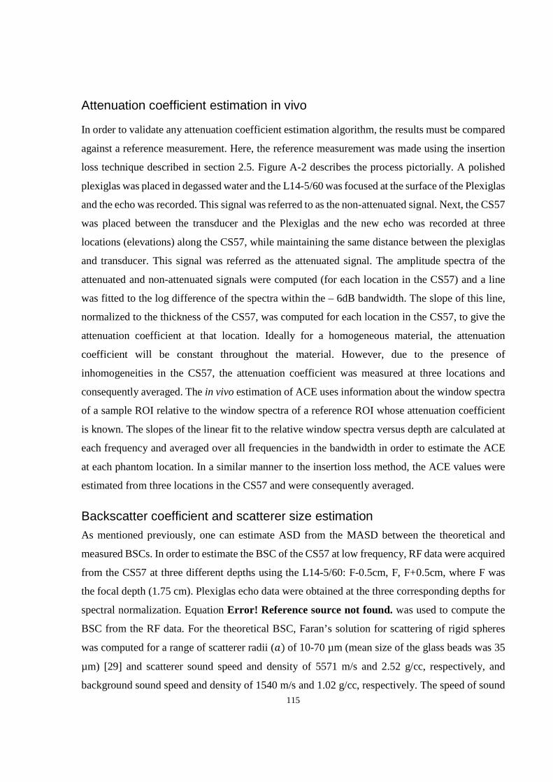
115

Attenuation coefficient estimation in vivo

In order to validate any attenuation coefficient estimation algorithm, the results must be compared

against a reference measurement. Here, the reference measurement was made using the insertion

loss technique described in section 2.5. Figure A-2 describes the process pictorially. A polished

plexiglas was placed in degassed water and the L14-5/60 was focused at the surface of the Plexiglas

and the echo was recorded. This signal was referred to as the non-attenuated signal. Next, the CS57

was placed between the transducer and the Plexiglas and the new echo was recorded at three

locations (elevations) along the CS57, while maintaining the same distance between the plexiglas

and transducer. This signal was referred as the attenuated signal. The amplitude spectra of the

attenuated and non-attenuated signals were computed (for each location in the CS57) and a line

was fitted to the log difference of the spectra within the – 6dB bandwidth. The slope of this line,

normalized to the thickness of the CS57, was computed for each location in the CS57, to give the

attenuation coefficient at that location. Ideally for a homogeneous material, the attenuation

coefficient will be constant throughout the material. However, due to the presence of

inhomogeneities in the CS57, the attenuation coefficient was measured at three locations and

consequently averaged. The in vivo estimation of ACE uses information about the window spectra

of a sample ROI relative to the window spectra of a reference ROI whose attenuation coefficient

is known. The slopes of the linear fit to the relative window spectra versus depth are calculated at

each frequency and averaged over all frequencies in the bandwidth in order to estimate the ACE

at each phantom location. In a similar manner to the insertion loss method, the ACE values were

estimated from three locations in the CS57 and were consequently averaged.

Backscatter coefficient and scatterer size estimation As mentioned previously, one can estimate ASD from the MASD between the theoretical and

measured BSCs. In order to estimate the BSC of the CS57 at low frequency, RF data were acquired

from the CS57 at three different depths using the L14-5/60: F-0.5cm, F, F+0.5cm, where F was

the focal depth (1.75 cm). Plexiglas echo data were obtained at the three corresponding depths for

spectral normalization. Equation Error! Reference source not found. was used to compute the

BSC from the RF data. For the theoretical BSC, Faran’s solution for scattering of rigid spheres

was computed for a range of scatterer radii (�)of 10-70 µm (mean size of the glass beads was 35

µm) [29] and scatterer sound speed and density of 5571 m/s and 2.52 g/cc, respectively, and

background sound speed and density of 1540 m/s and 1.02 g/cc, respectively. The speed of sound

116

and density values were based on values reported in previous studies involving a similar phantom

[32]. Finally, the MASD between each theoretical BSC and measured BSC was computed.

Results

Transducer characterization

Results of sound field simulations and experiments on the clinical transducer are presented in

Figure A-3. The detected image (Figure A-3A) shows a diffuse structure radiating from the focus

(14 mm). The lateral beam profile (Figure A-3B) shows a peak at the lateral center of the sound

field and a - 6dB line shows a -6 dB beamwidth of 0.36 mm (-0.18 to 0.18 mm). The axial

waveform (Figure A-3C) was used to obtain the reference power spectrum (Figure A-3D), from

which a Gaussian-fitted center frequency of 6.3 MHz and a -6 dB bandwith of 3-9 MHz were

obtained. The actual bandwidth used for data analysis was later adjusted to 3-8 MHz since the

experimentally measured phantom spectra showed large fluctuations above 8 MHz which was

likely related to noise. The depth of focus plot (Figure A-3E) shows the axial location of maximum

pressure (30 mm) and the -6 dB depth of focus is shown to start at 18 mm and extend beyond the

maximum depth of the image (4 mm). Pulse-echo measurements were limited to the most

commonly used imaging depth for data collections (clinical and phantom), which was 40 mm.

Sound fields were computed similarly for the other transducers using Field II and the resulting

parameters including center frequency, bandwidth, and lateral resolution are provided in Table A-

4.

Table A-4. Transducer specifications obtained from manufacturer and from simulations. Entries

with asterisks represents data obtained from simulations and entries without asterisks represent

data obtained from manufacturer specifications. DF = dynamic focusing.

Transducer

model

Number of

Elements

Center

Frequency

(MHz)

-6 dB

Bandwidth

(MHz)

Axial

Resolution

(µm)

Lateral

Resolution

(µm)

Focal

Length

(mm)

L14-5W/38 128 ~7* 3-9* 220* 360* DF

L14-5W/60 128 ~6* 3-8* 260* 360* DF

RMV 710B 1 ~25* 16-31* 70 140 15

117

Attenuation coefficient estimation in vivo

Results of attenuation coefficient estimation using insertion-loss and reference phantom methods

are presented in Figure A-4 and Figure A-5, respectively. Figure A-4 B and C present the echo

signals versus time for the non-attenuated and attenuated cases, respectively. As expected, it can

be observed that the insertion of the CS57 in the ultrasound propagation path has resulted in

amplitude diminishment (increased attenuation) as well as earlier echo arrival (increased speed of

sound). In terms of the spectra (Figure A-4 D and E) the attenuated spectrum is smaller in

amplitude and downshifted in center frequency compared to that of the non-attenuated case, which

is another effect of attenuation. From the linear fit on the log difference between the two amplitude

spectra and the known thickness of the CS57, the attenuation coefficient can be computed,

following equation 1.18. This value was determined to be 0.40 ± 0.03 dB/cm-MHz. The mean and

standard deviation were obtained by averaging the ACE values obtained from three different

locations (elevations) in the phantom.

Results of the attenuation coefficient estimation using the reference phantom method are presented

in Figure A4. In Figure A-4A a B-mode image of the CS57, with the transducer focus placed at

the center of the phantom, and the ROI used for attenuation estimation can be observed. The ROI

was segmented into 2×2mm windows (Figure A-4B) and depth-dependent changes in spectral

amplitude were computed. As expected from a homogeneous material, a reasonably strong linear

correlation was found between the spectral difference and depth at 5.5MHz, with R2=0.74, as

shown in Figure A-4C. The ACE of this CS57 was determined to be 0.47 ± 0.08 dB/cm-MHz. The

mean and standard deviation were obtained by averaging the ACE values obtained from three

different locations (elevations) in the CS57.

The obtained attenuation coefficient values of the CS57 using the two methods are shown in a bar

plot in Figure A-5. An unpaired t-test (two-tailed, 95% confidence interval) was performed to

compare the means of the ACEs obtained using the two methods, which revealed no statistically

significant difference (p=0.23).

118

Backscatter coefficient and scatterer size estimation in vivo

Results of measurement and theoretical prediction of the BSC and estimation of ASD of the CS57

are presented in Figure A-6. Before performing the MASD fitting, a scaling factor was applied to

the theoretical BSC in order to the match frequency-averaged values of the measured and

theoretical BSCs, as follows,

#$�(�]) = Ï#$(�]) = Ï %&9 �(�)*��(�, �)

where,

Ï = ∑ #$n(�])F]G�∑ #$(�])F]G�

As observed in Figure A-6A, the theoretical prediction of the BSC for 35 µm rigid spherical

scatterers fits the measured BSC with a R2 of 0.74. The BSC measurement shown here was

computed from RF echo data collected from the center of the CS57, however BSCs were computed

from two other locations (elevations) in the CS57 in order to estimate standard deviations in ASD

estimates. Figure A-6B presents a plot of R2 versus input scatterer radius (model input) for a range

of 10-70µm, demonstrating that the best fit (maximum R2) between the theoretical prediction and

measurement of the BSC occur when the scatterer radius is 36µm. Note that in the reference

phantom technique (equation 1.14) of BSC estimation, the MASD metric is used to determine the

ASD rather than R2. Nevertheless, both metrics result in the same ASD. The R2 value was shown

here since the values always range between 0 and 1 and therefore are more intuitive, compared to

the MASD metric.

119

A

B

Figure A-1. (A) Microphotograph of glass beads embedded in the gelatin-based phantom. Diameters were measured manually using the ruler in ImageJ software (National Institutes of Health, USA). Scale bar: 20 µm. (B) Bead size (radius) distribution with a least-squares-fitted normal distribution (black line). Bin size: 0.77µm (to obtain 10 equally spaced bins in the measurement range)

120

A

Figure A-2. Process of attenuation coefficient measurement using the insertion-loss technique in reflection mode. (A) Diagrams showing (left) reflection from a polished Plexiglas surface inside water medium and (right) reflection from the Plexiglas after passing through the attenuating medium (the phantom). (B) Non-attenuated pulse versus time, (C) Attenuated pulse versus time, (D) amplitude log spectra of the two pulses, and (E) Difference between attenuated log spectrum and non-attenuated log spectrum (dashed plot) with linear fit (solid plot) applied to the – 6 dB bandwidth (3-8 MHz).

121

A

B

lateral position, mm

axia

l dis

tan

ce, m

m

Detected image, log-compressed

-1 -0.5 0 0.5 1

13

14

15

16

17

18

-1 -0.5 0 0.5 1-40

-35

-30

-25

-20

-15

-10

-5

0

lateral position, mm

Max

imu

m P

ress

ure

Val

ue

(dB

re

max

imu

m)

TX/RX Lateral Beam Plot

122

C

D

E

17 18 19 20 21 22

-0.8

-0.6

-0.4

-0.2

0

0.2

0.4

0.6

0.8

1

time after transmit, microseconds

no

rmal

ized

pre

ssu

re

TX/RX Pressure vs. Time, at Lateral Location of Peak Pressure

0 2 4 6 8 10 12 14 16-120

-100

-80

-60

-40

-20

0

Frequency (MHz)

Ref

eren

ce P

ow

er S

pec

tru

m (

dB

re

max

)

SimulatedGaussian Fit

10 15 20 25 30 35-25

-20

-15

-10

-5

0

Depth (mm)

Max

imu

m P

ress

ure

Val

ue

(dB

re

max

imu

m)

MeasurementsCubic Spline Interpolation

123

Figure A-3. Point spread function of the L14-5W/60 transducer using a one-cycle 10 MHz square pulse excitation. (A) Detected B-mode image. (B) Plot of maximum pressure value versus lateral position at the focal depth (14 mm). The transient line indicates the - 6B beam width. (C) Received pressure versus time at the lateral center of the sound field. (D) Power spectrum of the plot in (C), with Gaussian fit shown in red and -6 dB bandwidth (3-8 MHZ) shown by the transient line. (E) Maximum pressure versus depth obtained by translating the transducer axially through the sound field. The data for this plot were obtained experimentally using a Plexiglas surface to generate the echoes. A

C

B

Figure A-4. Reference phantom method for estimation attenuation coefficient. (A) B-mode image of the phantom and ROI. (B) Magnified view of the ROI showing the windows in spectra are computed. (C) A plot of spectral difference versus depth at 5.5 MHz (center of the 3-8 MHz bandwidth). The spectral difference is averaged laterally.

124

Figure A-5 Comparison of attenuation coefficients values of the reference phantom estimated using the insertion-loss and reference phantom methods. Error bars represent standard deviation.

0.47

0.4

0

0.1

0.2

0.3

0.4

0.5

0.6

Spectral Difference Insertion-loss

Att

en

ua

tio

n c

oe

ffic

ien

t (d

B/c

m-M

Hz)

125

A

B

Figure A-6. BSC and scatterer size estimation of glass beads in a phantom. (A) Theoretical prediction (red) and measurement (blue) of the BSC as a function of frequency. (B) Coefficient of determination (R2) versus scatterer radius (model input).

10 20 30 40 50 60 70-2

-1.5

-1

-0.5

0

0.5

1 X: 36Y: 0.7421

Scatterer radius (µm)

R2

126

Discussion

In this chapter, sound field characterization was described, construction of a reference scattering

phantom was described, the reference phantom method was implemented and validated for in vivo

estimation of tissue attenuation coefficients, and the scatterer size estimation algorithm was

validated. Whereas the axial resolution of the clinical transducer is approximately 260 µm, it was

demonstrated that sub-resolution scatterers (35 µm) could be detected from measurement of the

frequency-dependence of the backscatter signal from a glass microsphere-embedded phantom. It

must be noted that the estimations of ACEs and ASDs are based on a homogeneous acoustic

scattering region, and in general, breast tumours present as non-homogeneous acoustic scattering

in ultrasound. In such cases, there will be large fluctuations in the spectral amplitude difference

with depth, which may result in negative attenuation coefficient estimates (which is physically

impossible), and the inclusion of tissue interfaces may result in poor scatterer model fits for ASD

estimation. One way to avoid negative ACE is to select multiple smaller ROIs within the tumour,

where the backscatter intensities are relatively homogeneous, and use the average ACE obtained

from the smaller ROIs. However, ASDs are estimated from 2 x 2 mm windows that make up the

tumour ROI. Thus, it is assumed that the windows are small enough to have homogeneous

scattering properties for ASD estimation.

127

References

[1] Canadian Cancer Society’s Advisory Committee on Cancer Statistics, “Canadian Cancer

Statistics 2013,” Toronto, 2013.

[2] B. Yalcin, “Overview on locally advanced breast cancer: defining, epidemiology, and

overview on neoadjuvant therapy.,” Exp. Oncol., vol. 35, no. 4, pp. 250–2, Dec. 2013.

[3] A. Kornecki, “Current status of breast ultrasound.,” Can. Assoc. Radiol. J., vol. 62, no. 1,

pp. 31–40, Feb. 2011.

[4] A. Karellas and S. Vedantham, “Breast cancer imaging: A perspective for the next

decade,” Med. Phys., vol. 35, no. 11, p. 4878, 2008.

[5] G. J. Whitman and E. A. Strom, “Workup and Staging of Locally Advanced Breast

Cancer,” Seminars in Radiation Oncology, vol. 19, no. 4. pp. 211–221, Oct-2009.

[6] E. A. Eisenhauer, P. Therasse, J. Bogaerts, L. H. Schwartz, D. Sargent, R. Ford, J.

Dancey, S. Arbuck, S. Gwyther, M. Mooney, L. Rubinstein, L. Shankar, L. Dodd, R.

Kaplan, D. Lacombe, and J. Verweij, “New response evaluation criteria in solid tumours:

revised RECIST guideline (version 1.1).,” Eur. J. Cancer, vol. 45, no. 2, pp. 228–47, Jan.

2009.

[7] K. Brindle, “New approaches for imaging tumour responses to treatment.,” Nat. Rev.

Cancer, vol. 8, no. 2, pp. 94–107, Feb. 2008.

[8] J. Chang, M. Ormerod, T. J. Powles, D. C. Allred, S. E. Ashley, and M. Dowsett,

“Apoptosis and proliferation as predictors of chemotherapy response in patients with

breast carcinoma.,” Cancer, vol. 89, no. 11, pp. 2145–52, Dec. 2000.

[9] R. Nishimura, T. Osako, Y. Okumura, M. Hayashi, Y. Totoyozumi, and N. Arima, “Ki-67

as a prognostic marker according to breast cancer subtype and a predictor of recurrence

time in primary breast cancer,” Exp. Ther. Med., vol. 1, no. 5, pp. 747–754, 2010.

[10] U. Sharma, K. K. A. Danishad, V. Seenu, and N. R. Jagannathan, “Longitudinal study of

the assessment by MRI and diffusion-weighted imaging of tumor response in patients with

128

locally advanced breast cancer undergoing neoadjuvant chemotherapy,” NMR Biomed.,

vol. 22, no. 1, pp. 104–113, 2009.

[11] M. Schelling, N. Avril, J. Nährig, W. Kuhn, W. Römer, D. Sattler, M. Werner, J. Dose, F.

Jänicke, H. Graeff, and M. Schwaiger, “Positron emission tomography using

[(18)F]Fluorodeoxyglucose for monitoring primary chemotherapy in breast cancer.,” J.

Clin. Oncol., vol. 18, no. 8, pp. 1689–95, Apr. 2000.

[12] O. Falou, H. Soliman, A. Sadeghi-Naini, S. Iradji, S. Lemon-wong, J. Zubovits, J. Spayne,

R. Dent, M. Trudeau, J. F. Boileau, F. C. Wright, M. J. Yaffe, and G. J. Czarnota, “Diffuse

Optical Spectroscopy Evaluation of Treatment Response in Women with Locally

Advanced Breast Cancer Receiving Neoadjuvant Chemotherapy,” Transl. Oncol., vol. 5,

no. 4, pp. 238–246, 2012.

[13] D. J. Coleman, F. L. Lizzi, R. H. Silverman, L. Helson, J. H. Torpey, and M. J. Rondeau,

“A model for acoustic characterization of intraocular tumors.,” Invest. Ophthalmol. Vis.

Sci., vol. 26, no. 4, pp. 545–50, Apr. 1985.

[14] E. J. Feleppa, A. Kalisz, J. B. Sokil-Melgar, F. L. Lizzi, T. Liu, A. L. Rosado, M. C. Shao,

W. R. Fair, Y. Wang, M. S. Cookson, V. E. Reuter, and W. D. W. Heston, “Typing of

prostate tissue by ultrasonic spectrum analysis,” IEEE Trans. Ultrason. Ferroelectr. Freq.

Control, vol. 43, no. 4, pp. 609–619, Jul. 1996.

[15] M. Yang, T. M. Krueger, J. G. Miller, and M. R. Holland, “Characterization of anisotropic

myocardial backscatter using spectral slope, intercept and midband fit parameters,”

Ultrason. Imaging, vol. 29, no. 2, pp. 122–34, Apr. 2007.

[16] J. Mamou, A. Coron, M. L. Oelze, E. Saegusa-Beecroft, M. Hata, P. Lee, J. Machi, E.

Yanagihara, P. Laugier, and E. J. Feleppa, “Three-dimensional high-frequency backscatter

and envelope quantification of cancerous human lymph nodes.,” Ultrasound Med. Biol.,

vol. 37, no. 3, pp. 345–57, Mar. 2011.

[17] F. L. Lizzi, M. Ostromogilsky, E. J. Feleppa, M. C. Rorke, and M. M. Yaremko,

“Relationship of Ultrasonic Spectral Parameters to Features of Tissue Microstructure,”

129

IEEE Trans. Ultrason. Ferroelectr. Freq. Control, vol. UFFC-33, no. 3, pp. 319–329,

May 1986.

[18] F. L. Lizzi, D. L. King, M. C. Rorke, J. Hui, M. Ostromogilsky, M. M. Yaremko, E. J.

Feleppa, and P. Wai, “Comparison of theoretical scattering results and ultrasonic data

from clinical liver examinations,” Ultrasound Med. Biol., vol. 14, no. 5, pp. 377–385, Jan.

1988.

[19] E. J. Feleppa, F. L. Lizzi, D. J. Coleman, and M. M. Yaremko, “Diagnostic spectrum

analysis in ophthalmology: a physical perspective.,” Ultrasound Med. Biol., vol. 12, no. 8,

pp. 623–31, Aug. 1986.

[20] C. J. Bruce, C. Pislaru, and J. F. Greenleaf, “Characterization of reperfused infarcted

myocardium from high-frequency intracardiac ultrasound imaging using homodyned K

distribution,” IEEE Trans. Ultrason. Ferroelectr. Freq. Control, vol. 49, no. 11, pp. 1530–

1542, Nov. 2002.

[21] M. L. Oelze, W. D. O’Brien, Jr, J. P. Blue, and J. F. Zachary, “Differentiation and

Characterization of Rat Mammary Fibroadenomas and 4T1 Mouse Carcinomas Using

Quantitative Ultrasound Imaging,” IEEE Trans. Med. Imaging, vol. 23, no. 6, pp. 764–

771, Jun. 2004.

[22] K. Nam, J. A. Zagzebski, and T. J. Hall, “Quantitative assessment of in vivo breast masses

using ultrasound attenuation and backscatter.,” Ultrason. Imaging, vol. 35, no. 2, pp. 146–

61, Apr. 2013.

[23] L. Sannachi, H. Tadayyon, A. Sadeghi-Naini, W. Tran, S. Gandhi, F. Wright, M. Oelze,

and G. Czarnota, “Non-invasive evaluation of breast cancer response to chemotherapy

using quantitative ultrasonic backscatter parameters.,” Med. Image Anal., vol. 20, no. 1,

pp. 224–236, Nov. 2014.

[24] H. Tadayyon, A. Sadeghi-Naini, L. Wirtzfeld, F. C. Wright, and G. Czarnota,

“Quantitative ultrasound characterization of locally advanced breast cancer by estimation

of its scatterer properties.,” Med. Phys., vol. 41, no. 1, p. 012903, Jan. 2014.

130

[25] B. Banihashemi, R. Vlad, B. Debeljevic, A. Giles, M. C. Kolios, and G. J. Czarnota,

“Ultrasound imaging of apoptosis in tumor response: novel preclinical monitoring of

photodynamic therapy effects.,” Cancer Res., vol. 68, no. 20, pp. 8590–6, Oct. 2008.

[26] R. M. Vlad, S. Brand, A. Giles, M. C. Kolios, and G. J. Czarnota, “Quantitative ultrasound

characterization of responses to radiotherapy in cancer mouse models.,” Clin. cancer Res.

an Off. J. Am. Assoc. Cancer Res., vol. 15, no. 6, pp. 2067–75, Mar. 2009.

[27] A. Sadeghi-Naini, O. Falou, H. Tadayyon, A. Al-Mahrouki, W. Tran, N. Papanicolau, M.

C. Kolios, and G. J. Czarnota, “Conventional Frequency Ultrasonic Biomarkers of Cancer

Treatment Response In Vivo,” Transl. Oncol., vol. 6, no. 3, pp. 234–243, Jun. 2013.

[28] A. Sadeghi-Naini, N. Papanicolau, O. Falou, J. Zubovits, R. Dent, S. Verma, M. Trudeau,

J. F. Boileau, J. Spayne, S. Iradji, E. Sofroni, J. Lee, S. Lemon-Wong, M. Yaffe, M. C.

Kolios, and G. J. Czarnota, “Quantitative ultrasound evaluation of tumor cell death

response in locally advanced breast cancer patients receiving chemotherapy.,” Clin.

Cancer Res., vol. 19, no. 8, pp. 2163–74, Apr. 2013.

[29] J. J. Faran, “Sound Scattering by Solid Cylinders and Spheres,” J. Acoust. Soc. Am., vol.

23, no. 4, p. 405, Jul. 1951.

[30] V. C. Anderson, “Sound Scattering from a Fluid Sphere,” J. Acoust. Soc. Am., vol. 22, no.

4, pp. 426–431, Jul. 1950.

[31] M. F. Insana, R. F. Wagner, D. G. Brown, and T. J. Hall, “Describing small-scale structure

in random media using pulse-echo ultrasound,” J. Acoust. Soc. Am., vol. 87, no. 1, pp.

179–192, Jan. 1990.

[32] J. J. Anderson, M. Herd, M. R. King, A. Haak, Z. T. Hafez, J. Song, M. L. Oelze, E. L.

Madsen, J. Zagzebski, W. D. O’Brien, and T. J. Hall, “Interlaboratory comparison of

backscatter coefficient estimates for tissue-mimicking phantoms.,” Ultrason. Imaging, vol.

32, no. 1, pp. 48–64, Jan. 2010.

[33] R. S. C. Cobbold, Foundations of Biomedical Ultrasound. Oxford University Press, 2006.

131

[34] M. F. Insana and T. J. Hall, “Parametric ultrasound imaging from backscatter coefficient

measurements: Image formation and interpretation,” Ultrason. Imaging, vol. 12, no. 4, pp.

245–267, Oct. 1990.

[35] L. X. Yao, J. A. Zagzebski, and E. L. Madsen, “Backscatter coefficient measurements

using a reference phantom to extract depth-dependent instrumentation factors,” Ultrason.

Imaging, vol. 12, no. 1, pp. 58–70, 1990.

[36] A. Sadeghi-Naini, N. Papanicolau, O. Falou, H. Tadayyon, J. Lee, J. Zubovits, A.

Sadeghian, R. Karshafian, A. Al-Mahrouki, A. Giles, M. C. Kolios, and G. J. Czarnota,

“Low-frequency quantitative ultrasound imaging of cell death in vivo.,” Med. Phys., vol.

40, no. 8, p. 082901, Aug. 2013.

[37] T. Varghese and K. D. Donohue, “Characterization of tissue microstructure scatterer

distribution with spectral correlation.,” Ultrason. Imaging, vol. 15, no. 3, pp. 238–54, Jul.

1993.

[38] K. Suzuki, N. Hayashi, Y. Sasaki, M. Kono, A. Kasahara, Y. Imai, H. Fusamoto, and T.

Kamada, “Evaluation of structural change in diffuse liver disease with frequency domain

analysis of ultrasound.,” Hepatology, vol. 17, no. 6, pp. 1041–6, Jun. 1993.

[39] U. R. Abeyratne and X. Tang, “Ultrasound scatter-spacing based diagnosis of focal

diseases of the liver,” Biomed. Signal Process. Control, vol. 2, no. 1, pp. 9–15, Jan. 2007.

[40] C. B. Machado, W. C. A. Pereira, M. Meziri, and P. Laugier, “Characterization of in vitro

healthy and pathological human liver tissue periodicity using backscattered ultrasound

signals.,” Ultrasound Med. Biol., vol. 32, no. 5, pp. 649–57, May 2006.

[41] S. M. Kay, Modern Spectral Estimation-Theory and Application. Prentice-hall, 1998.

[42] Y. Bige, Z. Hanfeng, and W. Rong, “Analysis of microstructural alterations of normal and

pathological breast tissue in vivo using the AR cepstrum.,” Ultrasonics, vol. 44, no. 2, pp.

211–5, Feb. 2006.

[43] C. Li, N. Duric, P. Littrup, and L. Huang, “In vivo breast sound-speed imaging with

ultrasound tomography.,” Ultrasound Med. Biol., vol. 35, no. 10, pp. 1615–28, Oct. 2009.

132

[44] F. T. D’Astous and F. S. Foster, “Frequency dependence of ultrasound attenuation and

backscatter in breast tissue.,” Ultrasound Med. Biol., vol. 12, no. 10, pp. 795–808, Oct.

1986.

[45] L. R. Taggart, R. E. Baddour, A. Giles, G. J. Czarnota, and M. C. Kolios, “Ultrasonic

characterization of whole cells and isolated nuclei.,” Ultrasound Med. Biol., vol. 33, no. 3,

pp. 389–401, Mar. 2007.

[46] Y. Labyed, T. a Bigelow, and B. L. McFarlin, “Estimate of the attenuation coefficient

using a clinical array transducer for the detection of cervical ripening in human

pregnancy.,” Ultrasonics, vol. 51, no. 1, pp. 34–9, Jan. 2011.

[47] M. L. Oelze and W. D. O’Brien, Jr, “Frequency-dependent attenuation-compensation

functions for ultrasonic signals backscattered from random media,” J. Acoust. Soc. Am.,

vol. 111, no. 5, pt1, p. 2308, 2002.

[48] R. M. Haralick, K. Shanmugam, and I. Dinstein, “Textural Features for Image

Classification,” IEEE Trans. Syst. Man. Cybern., vol. SMC-3, no. 6, pp. 610–621, Nov.

1973.

[49] “Graycomatrix: Create gray-level co-occurrence matrix from image,” 2015. [Online].

Available: http://www.mathworks.com/help/images/ref/graycomatrix.html.

[50] R. M. Vlad, N. M. Alajez, A. Giles, M. C. Kolios, and G. J. Czarnota, “Quantitative

ultrasound characterization of cancer radiotherapy effects in vitro.,” Int. J. Radiat. Oncol.

Biol. Phys., vol. 72, no. 4, pp. 1236–43, Nov. 2008.

[51] J. W. Hunt, A. E. Worthington, A. Xuan, M. C. Kolios, G. J. Czarnota, and M. D. Sherar,

“A model based upon pseudo regular spacing of cells combined with the randomisation of

the nuclei can explain the significant changes in high-frequency ultrasound signals during

apoptosis.,” Ultrasound Med. Biol., vol. 28, no. 2, pp. 217–26, Feb. 2002.

[52] M. C. Kolios, G. J. Czarnota, M. Lee, J. W. Hunt, and M. D. Sherar, “Ultrasonic spectral

parameter characterization of apoptosis.,” Ultrasound Med. Biol., vol. 28, no. 5, pp. 589–

97, May 2002.

133

[53] G. J. Czarnota, M. C. Kolios, H. Vaziri, S. Benchimol, F. P. Ottensmeyer, M. D. Sherar,

and J. W. Hunt, “Ultrasonic biomicroscopy of viable, dead and apoptotic cells.,”

Ultrasound Med. Biol., vol. 23, no. 6, pp. 961–5, Jan. 1997.

[54] G. J. Czarnota, M. C. Kolios, J. Abraham, M. Portnoy, F. P. Ottensmeyer, J. W. Hunt, and

M. D. Sherar, “Ultrasound imaging of apoptosis: high-resolution noninvasive monitoring

of programmed cell death in vitro, in situ and in vivo,” Br. J. Cancer, vol. 819, no. 3, pp.

520–527, Oct. 1999.

[55] S. Brand, E. C. Weiss, R. M. Lemor, and M. C. Kolios, “High frequency ultrasound tissue

characterization and acoustic microscopy of intracellular changes.,” Ultrasound Med.

Biol., vol. 34, no. 9, pp. 1396–407, Sep. 2008.

[56] R. H. Silverman, R. Folberg, M. J. Rondeau, H. C. Boldt, H. O. Lloyd, X. Chen, F. L.

Lizzi, T. A. Weingeist, and D. J. Coleman, “Spectral parameter imaging for detection of

prognostically significant histologic features in uveal melanoma.,” Ultrasound Med. Biol.,

vol. 29, no. 7, pp. 951–9, Jul. 2003.

[57] M. L. Oelze and W. D. O’Brien, “Application of three scattering models to

characterization of solid tumors in mice.,” Ultrason. Imaging, vol. 28, no. 2, pp. 83–96,

Apr. 2006.

[58] G. J. Czarnota and M. C. Kolios, “Ultrasound imaging of apoptosis: role of chromatin

structure and membrane configuration,” in Proc Am Inst Ultra Med Annu Meeting, 2001,

p. 117.

[59] K. A. Topp, J. F. Zachary, and W. D. O’Brien, Jr, “Quantifying B-mode images of in vivo

rat mammary tumors by the frequency dependence of backscatter,” J. ultrasound Med.,

vol. 20, no. 6, pp. 605–612, Jun. 2001.

[60] J. J. Anderson, M.-T. Herd, M. R. King, A. Haak, Z. T. Hafez, J. Song, M. L. Oelze, E. L.

Madsen, J. a Zagzebski, W. D. O’Brien, and T. J. Hall, “Interlaboratory comparison of

backscatter coefficient estimates for tissue-mimicking phantoms.,” Ultrason. Imaging, vol.

32, no. 1, pp. 48–64, Jan. 2010.

134

[61] K. Shung, Diagnostic ultrasound: Imaging and blood flow measurements. CRC Press,

2005.

[62] S. Brand, B. Solanki, D. B. Foster, G. J. Czarnota, and M. C. Kolios, “Monitoring of cell

death in epithelial cells using high frequency ultrasound spectroscopy.,” Ultrasound Med.

Biol., vol. 35, no. 3, pp. 482–93, Mar. 2009.

[63] T. M. Kolb, J. Lichy, and J. H. Newhouse, “Comparison of the Performance of Screening

Mammography , Physical Examination , and Breast US and Evaluation of Factors that

Influence Them : An Analysis of 27,825 Patient Evaluations,” Radiology, vol. 225, no. 1,

pp. 165–175, 2002.

[64] W. A. Berg, J. D. Blume, J. B. Cormack, E. B. Mendelson, D. Lehrer, M. Böhm-Vélez, E.

D. Pisano, R. A. Jong, W. P. Evans, M. J. Morton, M. C. Mahoney, L. H. Larsen, R. G.

Barr, D. M. Farria, H. S. Marques, K. Boparai, and I. A. 6666, “Combined screening with

ultrasound and mammography vs mammography alone in women at elevated risk of breast

cancer: Results of the First-Year Screen in ACRIN 6666,” JAMA, vol. 299, no. 18, pp.

2151–63, May 2008.

[65] A. V. Alvarenga, W. C. A. Pereira, A. F. C. Infantosi, and C. M. Azevedo, “Complexity

curve and grey level co-occurrence matrix in the texture evaluation of breast tumor on

ultrasound images,” Med. Phys., vol. 34, no. 2, pp. 379–387, Feb. 2007.

[66] Y.-Y. Liao, P.-H. Tsui, C.-H. Li, K.-J. Chang, W.-H. Kuo, C.-C. Chang, and C.-K. Yeh,

“Classification of scattering media within benign and malignant breast tumors based on

ultrasound texture-feature-based and Nakagami-parameter images,” Med. Phys., vol. 38,

no. 4, pp. 2198–207, 2011.

[67] W. J. Krzanowski, Principles of Multivariate Analysis: A User’s Perspective. New York:

Oxford University Press, 1988.

[68] E. L. Madsen, J. A. Zagzebski, R. A. Banjavie, and R. E. Jutila, “Tissue mimicking

materials for ultrasound phantoms.,” Med. Phys., vol. 5, no. 5, pp. 391–4, 1978.

135

[69] S. Tadjudin and D. A. Landgrebe, “Covariance estimation for limited training samples,” in

IGARSS ’98. Sensing and Managing the Environment. 1998 IEEE International

Geoscience and Remote Sensing. Symposium Proceedings. (Cat. No.98CH36174), 1998,

vol. 5, pp. 2688–2690 vol.5.

[70] H. Nasief, I. Rosado-Mendez, J. Zagzebski, and T. Hall, “Quantitative Ultrasound as an

Aid to Differentiate Benign From Malignant Breast Masses,” in AIUM (American Institute

of Ultrasound in Medicine) Annual Convention, 2013, p. S62.

[71] E. Franceschini, R. Guillermin, F. Tourniaire, S. Roffino, E. Lamy, and J.-F. Landrier,

“Structure factor model for understanding the measured backscatter coefficients from

concentrated cell pellet biophantoms.,” J. Acoust. Soc. Am., vol. 135, no. 6, pp. 3620–31,

2014.

[72] H. Tadayyon, L. Sannachi, and G. J. Czarnota, “Quantitative ultrasound monitoring of

breast tumor response to chemotherapy by analysis of frequency-dependent attenuation

and backscattered power,” in SPIE Medical Imaging, 2014, p. 904009.

[73] S. H. Giordano, “Update on locally advanced breast cancer,” ’The Oncol., vol. 8, no. 6,

pp. 521–530, Jan. 2003.

[74] L. X. Yao, J. A. Zagzebski, and E. L. Madsen, “Backscatter Coefficient Measurements

Using a Reference Phantom to Extract Depth-Dependent Instrumentation Factors,”

Ultrason. Imaging, vol. 12, no. 1, pp. 58–70, Jan. 1990.

[75] L. L. Fellingham and F. G. Sommer, “Ultrasonic Characterization of Tissue Structure in

the In Vivo Human Liver and Spleen,” IEEE Trans. Sonics Ultrason., vol. SU-31, no. 4,

pp. 418 – 428, 1984.

[76] K. A. Wear, R. F. Wagner, and B. S. Garra, “High resolution ultrasonic backscatter

coefficient estimation based on autoregressive spectral estimation using Burg’s

algorithm.,” IEEE Trans. Med. Imaging, vol. 13, no. 3, pp. 500–7, Jan. 1994.

[77] T. Cover and P. Hart, “Nearest neighbor pattern classification,” IEEE Trans. Inf. Theory,

vol. 13, no. 1, pp. 21–27, Jan. 1967.

136

[78] R. Rajan, A. Poniecka, T. L. Smith, Y. Yang, D. Frye, L. Pusztai, D. J. Fiterman, E. Gal-

Gombos, G. Whitman, R. Rouzier, M. Green, H. Kuerer, A. U. Buzdar, G. N. Hortobagyi,

and W. F. Symmans, “Change in tumor cellularity of breast carcinoma after neoadjuvant

chemotherapy as a variable in the pathologic assessment of response.,” Cancer, vol. 100,

no. 7, pp. 1365–73, Apr. 2004.

[79] A. K. Jain, R. P. W. Duin, and J. Mao, “Statistical pattern recognition: a review,” IEEE

Trans. Pattern Anal. Mach. Intell., vol. 22, no. 1, pp. 4–37, 2000.

[80] R. Peto and J. Peto, “Asymptotically Efficient Rank Invariant Test Procedures,” J. R. Stat.

Soc. Ser. A, vol. 135, no. 2, p. 185, 1972.

[81] S.-J. Dawson, D. W. Y. Tsui, M. Murtaza, H. Biggs, O. M. Rueda, S.-F. Chin, M. J.

Dunning, D. Gale, T. Forshew, B. Mahler-Araujo, S. Rajan, S. Humphray, J. Becq, D.

Halsall, M. Wallis, D. Bentley, C. Caldas, and N. Rosenfeld, “Analysis of circulating

tumor DNA to monitor metastatic breast cancer.,” N. Engl. J. Med., vol. 368, no. 13, pp.

1199–209, Mar. 2013.

[82] G. von Minckwitz, J. U. Blohmer, S. D. Costa, C. Denkert, H. Eidtmann, W. Eiermann, B.

Gerber, C. Hanusch, J. Hilfrich, J. Huober, C. Jackisch, M. Kaufmann, S. Kümmel, S.

Paepke, A. Schneeweiss, M. Untch, D. M. Zahm, K. Mehta, and S. Loibl, “Response-

guided neoadjuvant chemotherapy for breast cancer.,” J. Clin. Oncol., vol. 31, no. 29, pp.

3623–30, Oct. 2013.

[83] T. Hastie, R. Tibshirani, and J. Friedman, The Elements of Statistical Learning: Data

Mining, Inference, and Prediction, 2nd ed. Springer, 2011.

[84] D. P. Petrylak, C. M. Tangen, M. H. A. Hussain, P. N. Lara, J. A. Jones, M. E. Taplin, P.

A. Burch, D. Berry, C. Moinpour, M. Kohli, M. C. Benson, E. J. Small, D. Raghavan, and

E. D. Crawford, “Docetaxel and estramustine compared with mitoxantrone and prednisone

for advanced refractory prostate cancer.,” N. Engl. J. Med., vol. 351, no. 15, pp. 1513–20,

Oct. 2004.

137

[85] D. T. Miyamoto, L. V Sequist, and R. J. Lee, “Circulating tumour cells-monitoring

treatment response in prostate cancer.,” Nat. Rev. Clin. Oncol., vol. 11, no. 7, pp. 401–12,

Jul. 2014.

[86] E. J. Feleppa, “Ultrasonic tissue-type imaging of the prostate: implications for biopsy and

treatment guidance.,” Cancer Biomark., vol. 4, no. 4–5, pp. 201–12, Jan. 2008.

[87] P. Coupé, P. Hellier, X. Morandi, and C. Barillot, “Probe trajectory interpolation for 3D

reconstruction of freehand ultrasound,” Med. Image Anal., vol. 11, no. 6, pp. 604–15, Dec.

2007.

[88] B. Liu, H. D. Cheng, J. Huang, J. Liu, and T. XIanglong, “Fully automatic and

segmentation-robust classification of breast tumors based on local texture analysis,” Proc.

11th Jt. Conf. Inf. Sci., pp. 1–7, 2008.

[89] J. Shan, H. D. Cheng, and Y. Wang, “A novel segmentation method for breast ultrasound

images based on neutrosophic l-means clustering.,” Med. Phys., vol. 39, no. 9, pp. 5669–

82, Sep. 2012.

[90] R. Hickling, “Analysis of Echoes from a Solid Elastic Sphere in Water,” J. Acoust. Soc.

Am., vol. 34, no. 10, pp. 1582–1592, 1962.

[91] T. A. Bigelow, B. L. McFarlin, W. D. O’Brien, and M. L. Oelze, “In vivo ultrasonic

attenuation slope estimates for detecting cervical ripening in rats: Preliminary results,” J

Acoust Soc Am., vol. 123(3), no. 3, pp. 1794–1800, Mar. 2008.

[92] Y. Labyed and T. a Bigelow, “A theoretical comparison of attenuation measurement

techniques from backscattered ultrasound echoes.,” J. Acoust. Soc. Am., vol. 129, no. 4,

pp. 2316–24, Apr. 2011.

[93] D. P. Hruska and M. L. Oelze, “Improved parameter estimates based on the homodyned K

distribution.,” IEEE Trans. Ultrason. Ferroelectr. Freq. Control, vol. 56, no. 11, pp.

2471–81, Nov. 2009.