QUANTITATIVE NON-DESTRUCTIVE EVALUATION OF REBAR …
167
QUANTITATIVE NON-DESTRUCTIVE EVALUATION OF REBAR DIAMETER AND CORROSION DAMAGE IN CONCRETE USING GROUND PENETRATING RADAR by MD ISTIAQUE HASAN Presented to the Faculty of the Graduate School of The University of Texas at Arlington in Partial Fulfillment of the Requirements for the Degree of DOCTOR OF PHILOSOPHY THE UNIVERSITY OF TEXAS AT ARLINGTON MAY 2015
Transcript of QUANTITATIVE NON-DESTRUCTIVE EVALUATION OF REBAR …
QUANTITATIVE NON-DESTRUCTIVE EVALUATION OF REBAR DIAMETER AND
CORROSION DAMAGE IN CONCRETE USING
GROUND PENETRATING RADAR
by
MD ISTIAQUE HASAN
Presented to the Faculty of the Graduate School of
The University of Texas at Arlington in Partial Fulfillment
of the Requirements
for the Degree of
DOCTOR OF PHILOSOPHY
THE UNIVERSITY OF TEXAS AT ARLINGTON
MAY 2015

ii
Copyright © by Md Istiaque Hasan
All Rights Reserved

iii
Acknowledgements
I would like to express my profound appreciation to those who have contributed
to the completion of this dissertation. First and foremost, I would like to express my
utmost gratitude to my advisor and supervisor Dr. Nur Yazdani, who supported and
motivated me all through the time span of my PhD study and research. Without his
continuous support, guidance and mentoring, this work would not have been possible.
Also, thanks go to the members of my advisory committee, Dr. Shih-ho Chao, Dr.
Sahadat Hossain and Dr. Haiying Huang for their valuable time, guidance and
suggestions.
I will be always grateful to the Department of Civil Engineering at UT Arlington for
providing me with supports and facilities to perform my research work. I would like to
thank Dr. Yeonho Park and Eric Goucher for helping me acquiring materials and
experimental setup. Special thanks go to Paul Shover, Joseph Williams and Hram Mang
for helping me through the experimental phases of my research. I would like to thank my
friends at UT Arlington for making me feel at home at UT Arlington campus.
April 15, 2015
iv
Abstract
QUANTITATIVE NON-DESTRUCTIVE EVALUATION OF REBAR DIAMETER AND
CORROSION DAMAGE IN CONCRETE USING
GROUND PENETRATING RADAR
Md Istiaque Hasan, PhD
The University of Texas at Arlington, 2015
Supervising Professor: Nur Yazdani
The purpose of this study is to develop new methods for quantitative estimation
of rebar diameter and loss of area of rebar due to corrosion using Ground Penetrating
Radar (GPR). The existing methods of determining the rebar diameter using GPR are not
accurate and the existing methods for evaluating corrosion using GPR are qualitative.
The study included in this dissertation uses a 2.6 GHz antenna to estimate the diameter
of rebar using two different approaches. The approaches use digital image processing of
GPR ragargrams and maximum normalized reflection amplitude form the rebar to
estimate the diameter. A novel method to simulate corroded concrete beam specimen in
the lab at different level of corrosion using oil water emulsion and accelerated corrosion
of rebar in salt water solution.
The results of the diameter estimation using digital image processing shows that
the 2.6 GHz antenna can estimate the size of #4 (12 mm) and # 5 (16 mm) rebar with a
maximum error of 6.4%. Any diameter that is smaller than #4 (12 mm) and or larger than
#5 (16 mm) shows error of at least 18.4%. A relationship between the maximum
normalized reflection amplitudes from the GPR signal and the rebar diameter is

v
established. The relationship was verified using numerical modeling by using the
software GPRMAX.
Linear regression equations are developed to find the quantitative loss of area of
the rebar at different stages of corrosion from the accelerated corrosion test in the
laboratory. The regression equations are developed at three different dielectric constant
of the medium and three different depth of concrete cover. A guideline is proposed on
how to use the regression equation in the field to estimate the amount of area loss due to
corrosion.

vi
Table of Contents
Acknowledgements .............................................................................................................iii
Abstract .............................................................................................................................. iv
List of Illustrations ............................................................................................................... x
List of Tables ..................................................................................................................... xv
Chapter 1 Introduction......................................................................................................... 1
1.1 Introduction ............................................................................................................... 1
1.2 Problem Statement ................................................................................................... 3
1.3 Objectives ................................................................................................................. 4
1.4 Scope of the study .................................................................................................... 4
1.5 Organization of the Study ......................................................................................... 5
Chapter 2 Theory of GPR and Electromagnetic Theory ..................................................... 6
2.1 Introduction of GPR .................................................................................................. 6
2.2 System Design .......................................................................................................... 7
2.2.1 Range ................................................................................................................ 7
2.2.2 Velocity of propagation ...................................................................................... 8
2.2.3 Clutter ................................................................................................................ 8
2.2.4 Depth resolution ................................................................................................ 8
2.2.5 Plan resolution ................................................................................................... 9
2.3 Material properties and electromagnetic waves ....................................................... 9
2.4 GPR antenna .......................................................................................................... 10
Chapter 3 Literature Review ............................................................................................. 11
3.1 GPR Theory ............................................................................................................ 11
3.1.1 GPR Data Collection ....................................................................................... 12
3.1.2 Property of the medium ................................................................................... 15
vii
3.1.3 GPR Scan output............................................................................................. 16
3.1.4 Horizontal and Depth Resolution..................................................................... 18
3.2 Non-Destructive methods for measuring rebar diameter in concrete ..................... 19
3.2 Use of GPR is measuring diameter of rebar .......................................................... 21
3.3.1 Half Cell Potential Method (ASTM C876-09, 2014) ........................................ 29
3.3.2 Concrete Resistivity Method (ASTM WK-37880, 2012) .................................. 30
3.3.3 Linear Polarization Resistance (LPR) Method (ASTM G59-97,
2009)......................................................................................................................... 31
3.4 Corrosion Detection with GPR ................................................................................ 32
3.5 Other methods on corrosion detection ................................................................... 37
3.6 Limitation of previous study and significance of the research ................................ 39
Chapter 4 Effect of various GPR parameters on rebar diameter estimation .................... 41
4.1 Introduction ............................................................................................................. 41
4.2 Materials and Equipment Used .............................................................................. 41
4.2.1 Rebars ............................................................................................................. 41
4.2.2 GPR System .................................................................................................... 42
4.3 Casting of the Beams ............................................................................................. 44
4.4 GPR scanning and data collection ......................................................................... 46
4.5 GPR Data Processing ............................................................................................ 49
4.6 Effect of maximum amplitude on rebar diameter .................................................... 51
4.6.1 Effect of maximum amplitude on rebar diameter ............................................ 53
4.6.2 Effect of maximum amplitude on rebar diameter at different depth ................ 54
4.6.3 Effect of maximum amplitude ratio on rebar diameter .................................... 55
4.6.4 Diameter Estimation from maximum positive amplitude ................................. 58
4.7 Diameter Estimation using Empirical Approach ..................................................... 60

viii
4.7 Discussion .............................................................................................................. 67
Chapter 5 Effect of various GPR parameters on corroded rebar in concrete ................... 69
5.1 Introduction ............................................................................................................. 69
5.2 Oil Tank as a substitute of concrete beam specimen............................................. 69
5.2.1 Preparation of oil tank ..................................................................................... 70
5.2.2 Dielectric Constant of Different Tanks ............................................................. 73
5.3 Validation of oil tank as a substitute of concrete beam .......................................... 75
5.4 Plot of the collected data to verify the performance of the oil tanks ....................... 76
5.5 Accelerated corrosion test ...................................................................................... 82
5.6 Corrosion Tank ....................................................................................................... 84
5.7 Collected Data from the corroded rebars ............................................................... 87
5.8 Effect of corrosion on GPR responses ................................................................... 91
5.9 Relationship between amount of corrosion and GPR responses ........................... 95
5.10 Proposed method to estimate the amount of corrosion........................................ 98
5.11 Monitoring accelerated corrosion process in a real concrete beam ..................... 99
5.12 Results of accelerated corrosion in a real concrete beam ................................. 102
5.13 Discussion .......................................................................................................... 105
Chapter 6 Numerical modeling ....................................................................................... 107
6.1 Introduction ........................................................................................................... 107
6.2 Basic concepts of GPR modeling ......................................................................... 107
6.3 Assumption of GPR modeling using GPRMAX .................................................... 111
6.4 Input file commands ............................................................................................. 111
6.4.1 Units .............................................................................................................. 112
6.4.2 Media and object construction ....................................................................... 112
6.4.3 Antenna modeling.......................................................................................... 113

ix
6.4.4 Domain and time window .............................................................................. 114
6.5 Creating command file and running the model ..................................................... 115
6.6 Output of Simulation ............................................................................................. 118
6.7 Effect of size of the rebar and dielectric permittivity on simulated GPR
Response .................................................................................................................... 121
6.8 Validation of the numerical model compared to real GPR data ........................... 123
6.8 Effect of dielectric permittivity on simulated GPR Response ............................... 125
6.8 Effect of frequency and the size of the element ................................................... 128
6.9 Discussion ............................................................................................................ 133
Chapter 7 Conclusions and Recommendations ............................................................. 135
7.1 Introduction ........................................................................................................... 135
7.2 Conclusions .......................................................................................................... 135
7.3 Future Research ................................................................................................... 139
Appendix A GPRMAX2D Output Signal .......................................................................... 141
Appendix B MATLAB CODES FOR GPRMAX2D .......................................................... 146
References ...................................................................................................................... 148
Biographical Information ................................................................................................. 152

x
List of Illustrations
Figure 3-1 Schematic diagram of generic GPR system .................................................... 11
Figure 3-2 Ground coupled and air-launched antenna
(GSSI Concrete Handbook, 2015) .................................................................................... 12
Figure 3-3 GPR Surveying methods (Warren, 2009) ........................................................ 13
Figure 3-4 Antenna polarization (GSSI Concrete Handbook, 2015) ................................ 14
Figure 3-5 Direct coupling or direct wave form the surface
(GSSI Concrete Handbook, 2015) .................................................................................. 16
Figure 3-6 GPR A-Scan .................................................................................................... 17
Figure 3-7 GPR B-Scan or radargram .............................................................................. 17
Figure 3-8 GPR C-Scan or 3-D view (GSSI Concrete Handbook, 2015) ......................... 18
Figure 3-9 Reluctance based and eddy current based cover meters
(Washer, G. A. 2013) ...................................................................................................... 19
Figure 3-10 Radiograph of spiral steel in concrete encircling high strength tendons ....... 20
Figure 3-11 GPR hyperbola traces (Shihab and Al-Nuaimy, 2005) .................................. 21
Figure 3-12 Relationship between rebar diameter and maximum normal amplitude
at different depths (Utsi and Utsi, 2004) ......................................................................... 23
Figure 3-13 Physical model of GPR scan of rebar in concrete (Chang et al. 2009) ...... 24
Figure 3-14 Antenna orientations: (a) co-polarized;
(b) cross-polarized (Leucci, G. 2012) .............................................................................. 25
Figure 3-15 Correlation between bar diameter and amplitude ratio (Leucci, G. 2012) .... 26
Figure 3-16 RCS ratio for three different antenna
frequencies (Zanzi and Arosio, 2013) ............................................................................. 27
Figure 3-17 Electrochemical Reactions during corrosion of reinforcing steel in
concrete (Ahmad, 2003).................................................................................................. 28

xi
Figure 3-18 Corrosion of steel reinforcement in concrete
(The Helpful Engineer, 2010) .......................................................................................... 29
Figure 3-19 Half cell potential mapping (Millard and Sadowski, 2009) ............................. 30
Figure 3-20 Concrete resistivity method (Millard and Sadowski, 2009) ........................... 31
Figure 3-21 Linear polarization resistance measurement
(Millard and Sadowski, 2009 ........................................................................................... 31
Figure 3-22 Accelerated corrosion set up, (a) plan, (b) section (Lai et al. 2012).............. 33
Figure 3-23 Specimen in corrosion tank with anode
and cathode rebars (Lai et al. 2012) ............................................................................... 33
Figure 3-24 GPR A-Scan in time domain with one in. (25 mm) concrete cover: (a) 2.6
GHz antenna; (b) 1.5 GHz antenna (Lai et al. 2012) ........................................................ 34
Figure 3-25 Increase in rebar amplitude with time (Lai et al., 2012) ................................ 35
Figure 3-26 DW, RW and peak to peak amplitude (Hong et al., 2014) ........................... 36
Figure 3-27 Changes in peak to peak amplitude for
RW from rebar (Hong et al., 2014) .................................................................................. 36
Figure 3-28 Correlation between normalized amplitude and the amount of
mass loss (Zhan el a. 2011) ............................................................................................ 37
Figure 3-29 Change of dielectric permittivity ɛ′ (a) and ɛ″ (b) of different corrosion
product with increasing frequency (Kim et al., 2010) ...................................................... 38
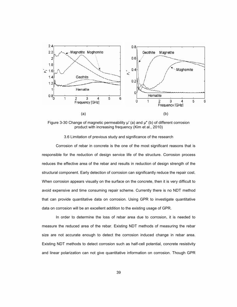
Figure 3-30 Change of magnetic permeability μ′ (a) and μ″ (b) of different
corrosion product with increasing frequency (Kim et al., 2010) ...................................... 39
Figure 4-1 Different diameters of the rebar ....................................................................... 42
Figure 4-2 GPR System used in this study ....................................................................... 44
Figure 4-3 Schematic diagram of the beam specimen .................................................... 45
Figure 4-4 Casting of the beam specimens ...................................................................... 46
xii
Figure 4-5 Antenna orientation, (a) Normal, (b) Parallel ................................................... 47
Figure 4-6 GPR scanning of beam specimen with #8 (25 mm) diameter rebar ............... 47
Figure 4-7 Steps of GPR data processing in RADAN ....................................................... 50
Figure 4-8 Amplitude vs rebar size at 1 in. (25 mm) cover ............................................... 53
Figure 4-9 Amplitude vs rebar size at 2 in. (50 mm) cover ............................................... 54
Figure 4-10 Amplitude vs rebar diameter at different depths [1 in. (25 mm),
2 in. (50 mm), and 3 in.(75 mm)] ..................................................................................... 55
Figure 4-11 Amplitude ratio vs rebar diameter for 1 in. (25 mm) concrete cover ............. 56
Figure 4-12 Amplitude ratio vs rebar diameter for 2 in. (50 mm) concrete cover ............. 57
Figure 4-13 Amplitude ratio vs rebar diameter for 3 in. (75 mm) concrete cover ............. 57
Figure 4-14 Rebar diameter vs maximum normalized amplitude for
numerical and experimental data .................................................................................... 60
Figure 4-15 Elliptical cone and the radius of energy footprint E (Chang et al. 2009) ....... 61
Figure 4-16 GPR radargram in Matlab .............................................................................. 63
Figure 4-17 Digitized image in Matlab .............................................................................. 63
Figure 4-18 Conversion of digital image to alpha numeric codes ..................................... 64
Figure 5-1 Oil tank as a substitute of concrete beam ....................................................... 70
Figure 5-2 Arrangement to hold rebars in oil tank to simulate concrete cover ................. 71
Figure 5-3 Oil water emulsion tank ................................................................................... 72
Figure 5-4 Determination of Dielectric Constant of oil tank with steel plate ..................... 73
Figure 5-5 Radargrams of the three tanks ........................................................................ 74
Figure 5-6 GPR Radargram data collected form oil tank. ................................................. 76
Figure 5-7 Rebars used in the oil and emulsion tanks ...................................................... 77
Figure 5-8 Amplitude vs cover depth for #3 (10 mm) rebar .............................................. 79
Figure 5-9 Amplitude vs cover depth for #4 (12 mm) rebar .............................................. 79

xiii
Figure 5-10 Amplitude vs cover depth for #5 (16 mm) rebar ............................................ 80
Figure 5-11 Amplitude vs dielectric constant for #3 (10 mm) rebar .................................. 81
Figure 5-12 Amplitude vs dielectric constant for #4 (12 mm) rebar .................................. 81
Figure 5-13 Amplitude vs dielectric constant for #5 (16 mm) rebar .................................. 82
Figure 5-14 Schematic diagram of GPR scanning of corroded rebar ............................... 84
Figure 5-15 Corrosion tank for accelerated corrosion ...................................................... 85
Figure 5-16 DC power source and 10 KΩ resistor ............................................................ 86
Figure 5-17 Three corroded rebars with a non-corroded rebar on the left ....................... 87
Figure 5-18 Oil emulation tanks for corroded rebar .......................................................... 89
Figure 5-19 GPR Data collection from the corroded rebar in oil emulsion tank ............... 89
Figure 5-20 TWTT vs cover depth for different corroded rebar in tank-1(ε=2.73) ............ 91
Figure 5-21 TWTT vs cover depth for different corroded rebar in tank-2 (ε=5.47) ........... 92
Figure 5-22 TWTT vs cover depth for different corroded rebar in tank-3 (ε=9.3) ............. 92
Figure 5-23 Maximum amplitude vs cover depth for different corroded
rebar in tank-1 (ε=2.73) ................................................................................................... 93
Figure 5-24 Maximum amplitude vs cover depth for different
corroded rebar in tank-2 (ε=5.47) ................................................................................... 94
Figure 5-25 Maximum amplitude vs cover depth for different
corroded rebar in tank-3 (ε=9.3)...................................................................................... 94
Figure 5-26 Maximum amplitude vs percentage area loss in tank-1 (ε = 2.73) ................ 96
Figure 5-27 Maximum amplitude vs percentage area loss in tank-2 (ε = 5.47) ................ 97
Figure 5-28 Maximum amplitude vs percentage area loss in tank-3 (ε = 9.3) .................. 97
Figure 5-29 Concrete beam with four #5 (16 mm) rebar in 5% salt water solution ........ 100
Figure 5-30 Experimental set-up of accelerated corrosion ............................................. 101
Figure 5-31 Daily data collection to monitor corrosion .................................................... 101

xiv
Figure 5-32 Typical GPR Scan of the sample beam ...................................................... 102
Figure 5-33 The corroded state of the two rebars in the middle after 30 days ............... 102
Figure 5-34 Maximum amplitude vs time for rebar-1 ...................................................... 104
Figure 5-35 Maximum amplitude vs time for rebar-2 ..................................................... 104
Figure 6-1 Yee cell used in FTDT method (Giannopoulos, 2005) .................................. 109
Figure 6-2 GPRMAX model of a half space with ABC (Giannopoulos, 2005) ................ 110
Figure 6-3 Normalized ricker excitation function (Giannopoulos, 2005) ......................... 116
Figure 6-4 Geometry of the physical model generated in MATLAB ............................... 119
Figure 6-5 B-Scan of the model generated in MATLAB ................................................ 120
Figure 6-6 The A-Scan trace form the GPR Simulation of a rebar in concrete .............. 121
Figure 6-7 Simulated GPR traces from six different rebars by GPRMAX ...................... 122
Figure 6-8 Normalized amplitude traces from rebars of
different sizes from numerical model ............................................................................ 123
Figure 6-9 Simulated GPR traces of 16 mm (#5) rebar
at different dielectric medium ........................................................................................ 127
Figure 6-10 Simulated normalized GPR traces of 16 mm (#5) rebar
at different dielectric medium ........................................................................................ 128
Figure 6-11 Amplitude vs travel time for different frequencies ....................................... 129
Figure 6-12 Maximum amplitude vs antenna frequency from the numerical model ....... 130
Figure 6-13 Amplitude vs time traces for different
mesh sizes of the numerical model ............................................................................... 131
Figure 6-14 Reflection amplitudes from rebar for different sizes of
elements in the numerical model .................................................................................. 132
Figure 6-15 Maximum amplitudes vs size of the element in numerical model ............... 133
xv
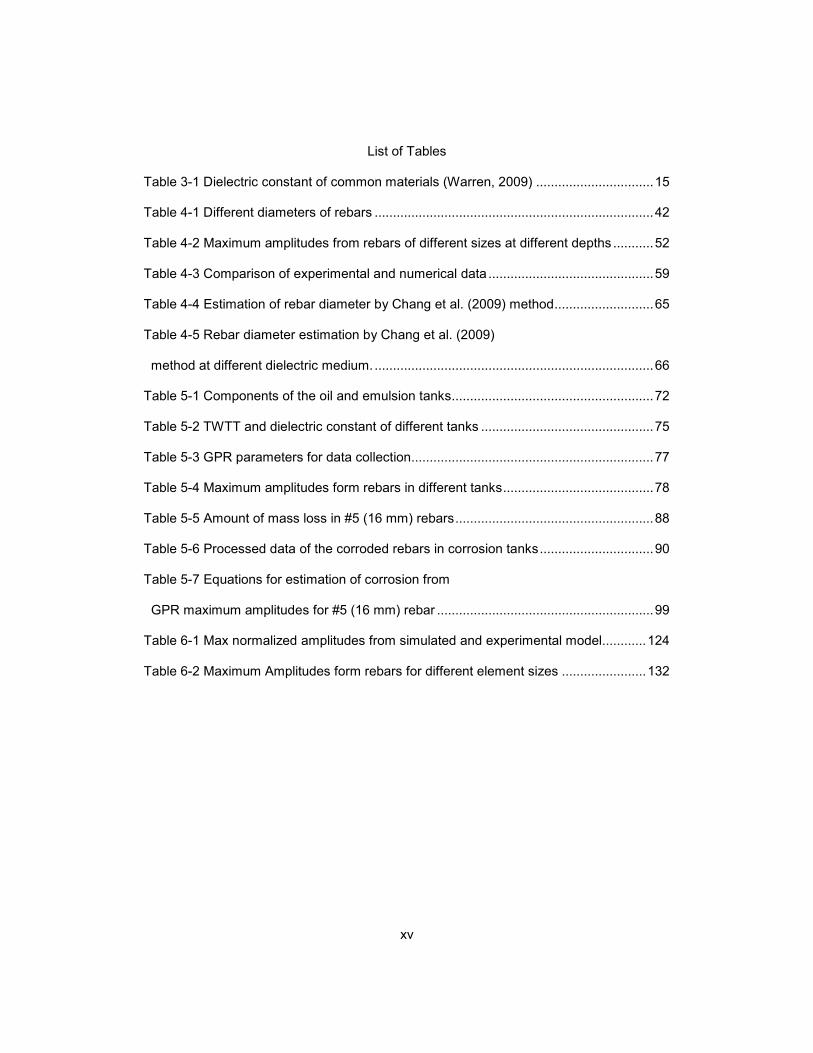
List of Tables
Table 3-1 Dielectric constant of common materials (Warren, 2009) ................................ 15
Table 4-1 Different diameters of rebars ............................................................................ 42
Table 4-2 Maximum amplitudes from rebars of different sizes at different depths ........... 52
Table 4-3 Comparison of experimental and numerical data ............................................. 59
Table 4-4 Estimation of rebar diameter by Chang et al. (2009) method ........................... 65
Table 4-5 Rebar diameter estimation by Chang et al. (2009)
method at different dielectric medium. ............................................................................ 66
Table 5-1 Components of the oil and emulsion tanks ....................................................... 72
Table 5-2 TWTT and dielectric constant of different tanks ............................................... 75
Table 5-3 GPR parameters for data collection.................................................................. 77
Table 5-4 Maximum amplitudes form rebars in different tanks ......................................... 78
Table 5-5 Amount of mass loss in #5 (16 mm) rebars ...................................................... 88
Table 5-6 Processed data of the corroded rebars in corrosion tanks ............................... 90
Table 5-7 Equations for estimation of corrosion from
GPR maximum amplitudes for #5 (16 mm) rebar ........................................................... 99
Table 6-1 Max normalized amplitudes from simulated and experimental model............ 124
Table 6-2 Maximum Amplitudes form rebars for different element sizes ....................... 132

1
Chapter 1
Introduction
1.1 Introduction
Ground Penetrating Radar (GPR) is a non-destructive testing equipment
normally used for geophysical investigation. However, use of GPR in concrete structure
investigation has progressed substantially. GPR can produce 2D and 3D images of the
concrete subsurface and different features, such as rebars, conduits, cracks and voids.
Such hidden features in the subsurface can be detected from the GPR data output. As
non-destructive testing (NDT) is becoming popular in the field of structural and materials
engineering, researchers worldwide are exploring additional usage of GPR. Every year,
billions of dollars are being spent on repair and rehabilitation of existing structures,
especially highways and bridges. According to ASCE 2013 report card for America’s
infrastructure, one in nine of the nation’s bridges are structurally deficient. Every year
12.8 billion dollars are being spent for the repair and maintenance of the bridges in the
U.S.A.. To determine the repair scheme of an existing structure, accurate and robust
condition assessment is necessary. The repair cost can be substantially reduced and
service life and safety can be increased, if potential damage or failure threat to a
structure can be predicted ahead of time .
GPR has been widely used to map concrete deterioration of bridge decks (Parillo
and Haggan, 2005). GPR is also used to find location and depth of rebar in concrete. As
RADAR wave is very sensitive to moisture, GPR is also used to find location of high
moisture content area on a concrete surface. So far, the existing usages of GPR
produces mainly qualitative data. Now attention of the GPR practitioners are focused on
retrieving more quantitative data from GPR scan to extend its efficiency on NDT of
concrete. GPR can easily detect rebar locations embedded in concrete, but more
2
quantitative information about rebars, such as mass loss of the rebar due to corrosion,
cannot be directly measured form direct GPR scan output. GPR can collect data quicker
than any other existing NDT methods. If quantitative data, such as amount of corrosion
and rebar diameter, can be retrieved from GPR scan, it will be an excellent addition to the
usage of GPR in practical applications. When engineers work on addition or renovation
projects, the as-built drawings are sometimes not available or reliable. Having additional
information on rebars from non-destructive manner would surely be helpful in evaluating
the existing strength of the structure.
Concrete structures could be exposed to exterior environment which could be
very aggressive due to the presence of high temperature, chloride, carbon dioxide,
water, sulphides and other chemicals. These aggressive agents may cause rebar
corrosion and ultimately damage the structural integrity. Repair costs of such damages
are normally very high. That is why preemptive repair and retrofitting is necessary to
prevent the structure from corrosion damage and extend the service life of the structure.
Several rebar locators are commercially available to determine the concrete
cover and rebar diameter. These rebar locators are designed according to the magnetic
pulse induction method. The application of such techniques are limited to smaller rebar
diameters and smaller concrete covers. Moreover, the magnetic pulse rebar locator
cannot collect data as quickly as GPR. A few past research studies e concentrated on
rebar diameter determination form GPR scan in a number of different ways. Utsi (2004),
Leucci (2012) and Zanzi and Arosio (2013) have tried to find rebar diameter in concrete
by comparing GPR responses from two orientations of the antenna polarized by 90
degree angle. These methods can predict rebar diameter with an accuracy of 20%.
Shihab and Al-Nuaimy (2005) tried to find GPR rebar diameter by mathematical model
based on hyperbola fitting to GPR data; this method has limited field application. Chang

3
(2009) developed an algorithm and tried to find rebar diameter using digital image
processing. However, this method is similar to an empirical approach and only limited
number of variables were considered. From the existing literature, it is clear that the GPR
based method of rebar diameter estimation can be greatly improved by considering a
number of variables that can affect calculation. The GPR parameters that affect the
diameter of the rebar can be used to study the thinning of the rebar in concrete due to
corrosion. In this study, the electrochemical corrosion process will be simulated in the
laboratory in an accelerated environment whereas real corrosion takes years to happen.
The GPR response from those corroded rebar with be studied to establish a relationship
between a GPR parameter and the amount of corrosion.
1.2 Problem Statement
Current GPR technology can be used to determine the presence of corrosion.
The relation between the corrosion process and GPR response is studied by Lai et al.
(2010). GPR parameters, such as two way travel time, maximum rebar amplitude were
changed with the progress of corrosion (Lai et al., 2010). GPR had been used to detect
the presence of corrosion but the results of such studies were qualitative (Martino el at.,
2014). No significant study on the quantitative estimation of corrosion was performed.
Moreover majority of the existing study are based on lower frequency antennas, i. e. 1.6
GHz or 2 GHz. It is imperative to determine a quantitative relationship between the GPR
parameter and the amount of corrosion using a higher frequency antenna.

4
1.3 Objectives
The main objectives of the study are as follows:
• Determination of GPR parameter that can detect decrease of diameter of
rebar due to corrosion induced mass loss.
• Effect of dielectric constant of the concrete on the GPR corrosion
parameter
• Effect of concrete cover of the rebar on GPR corrosion parameter
• Perform accelerated corrosion on rebar in salt water tank
• The GPR response of corroded rebar in oil emulsion tank
• Verification of the emulsion tank data by performing corrosion on real
reinforced concrete beam
• Proposing a relation between amount of corrosion and corresponding
GPR parameter
• Numerical modeling of the experimental data to verify the performance in
the experimental phase
1.4 Scope of the study
The results presented in this study have some limitations. The only antenna used
in the study is GSSI (Geophysical Survey System, Inc.) 2600 MHz antenna. So the effect
of antenna frequency on GPR response is not included in this study. The amount of
energy dissipated by an antenna depends on the design of the antenna, which is
designer specific. So, two antennas of same frequency from different providers can
produce differences in output. This study is only valid for the antenna manufactured my
GSSI. The corrosion study is done based on a number of assumptions which may not be
the actual scenario. GPR wave can illuminate only one side of the rebar during a scan.
So, if the corrosion is present on the other side of the rebar, GPR response will not be

5
able to detect it. However, in most cases, corrosion is supposed to happen on the side
with the least amount of cover, typically facing the GPR. The numerical study was
performed to verify the behavior of the experimental results. The numerical models were
not calibrated exactly with the experimental model. In this study, the different factors that
can be influential in calculating rebar diameter through GPR scan will be studied. The
factors that affect the change of size of the rebar will be used to detect the amount of
corrosion damage of the rebar.
1.5 Organization of the Study
The organization of the remainder of this dissertation is as follows. Theory of
GPR and electromagnetic theory is discussed in brief in Chapter 2. The literature review
on the usage of GPR on diameter estimation and detection are discussed in Chapter 3.
The review of existing work on the application of GPR on detecting and assessing
corrosion damage is also discussed in Chapter 3. In Chapter 4, the parameters that affect
the diameter estimation of rebar in concrete are presented. In Chapter 5, oil emulsion
tanks are presented as a substitute of concrete beams. The emulsion tanks are used to
investigate the effect of dielectric property on GPR response. The GPR response from
corroded rebar obtained from accelerated corrosion tests are also presented. The
changes of GPR response with the progress of corrosion in a real concrete beam are
studied as well. Chapter 6 discusses the numerical modeling of a rebar in concrete using
Finite Difference Time Domain FDTD method. The electromagnetic simulation of the
rebar embedded in concrete is presented in this chapter. The response of the numerical
value are used to support the experimental values obtained in Chapter 5. Finally,
conclusions and recommendations are presented in Chapter 7.

6
Chapter 2
Theory of GPR and Electromagnetic Theory
2.1 Introduction of GPR
There are several methods to create an image of the subsurface in order to
detect and locate buried objects. The methods that are already being used as subsurface
detection techniques are seismic, electric resistivity, nucleonic, gravity surveying,
thermographic and electromagnetic methods. Among all these methods, GPR is most
popular among the engineers and practicing scientists because of its range of
specializations. The term GPR refers to a range of electromagnetic techniques which is
designed primary for locating objects of interface. The design philosophy primarily
depends on type of the target and the material properties. The range of application of
GPR is very diverse and the quality of this technique is increasing with the development
of more sophisticated signal recovery techniques, system design and operating practices.
GPR can detect dielectric discontinuity and the target can be classified according
to the geometry of the target such as planner surface, cylindrical object, cuboidal objects
etc. GPR system can be preferentially designed to detect a particular type of target. The
signal attenuation and the frequency of the antenna are the two major factors in GPR
system design for a particular application. The material that possesses a high magnitude
of low frequency conductivity will have higher degree of signal attenuation. The
attenuation can be decreased by using a lower frequency but compromising with the
resolution. According to Daniels (2004), successful operation of GPR depends on the
following factors:
(a) efficient coupling of GPR waves to the ground
(b) adequate penetration of the GPR wave to the target with least attenuation
(c) a significant amount of backscattered signal from the target

7
(d) an adequate bandwidth of the detected signal for good resolution and low
noise levels.
GPR technique is usually used to detect backscattered radiation from the target
although forward scattering is also possible in some application but at least one antenna
needs to be buried into the ground. The depth and resolution needs to be clearly defined
according to the application because this controls the frequency and the bandwidth of the
antenna.
2.2 System Design
The design of GPR depends on a number of factors that influence the ability to
detect and the resolution. For successful operation of GPR, an adequate signal to clutter
ratio, signal to noise ratio, adequate spatial resolution and adequate depth resolution
must be confirmed. The main factors in system design are range, velocity of
propagation, clutter, depth resolution and plan resolution.
2.2.1 Range
The range of GPR depends on three factors. They are material loss, spreading
loss and reflection loss. The signal that is detected by the receiver antenna goes through
several types of losses. For a particular distance from the antenna to the target, the total
path loss (LT) is shown in the following Eq. (2.1) (Daniels, 2004).
�� = �� + �� + ��� + �� + � + �� + ��� (2.1)
Where,
��= antenna efficiency loss
��= antenna mismatch loss
���= transmission loss from air to material
��= retransmission loss from material to air
��= antenna spreading loss
8
�= attenuation loss from material
���= target scattering loss
2.2.2 Velocity of propagation
If the velocity of the propagation of the electromagnetic wave is known, it is
possible to measure the depth of thickness of the target. If the material is homogenous
and isotropic, the relative propagation velocity � can be found from Eq. (2.2)
� = �√ɛ� (2.2)
The depth or thickness d can be found from the following Eq. (2.3)
� = � � (2.3)
where, ɛ� is the relative permittivity and t is the two way travel time. The velocity
can be measured from a hyperbolic signature or from common depth point method.
Propagation velocity increases with increasing relative dielectric permittivity. The velocity
slows down in a material and the wavelength also decreases.
2.2.3 Clutter
Cutter is unwanted signals in the GPR scan that have similar scattering
characteristics to the real target. Clutter can be caused by breakthrough between the
transmitter and the receiver antenna. The multiple reflections between the ground surface
and the antenna also create clutter. The amount of clutter varies on the type of antenna
configurations.
2.2.4 Depth resolution
Depth resolution is important where a number of different types of targets are
targeted with the GPR within a given depth. A signal with a wider bandwidth is required to
distinguish between the different types of targets. The bandwidth of the received signal is

9
more important than that of the transmitting signal. The receiver bandwidth can be
determined by the power spectrum of the received signal.
2.2.5 Plan resolution
Plan resolution of radar is important when there are multiple targets at the same
depth. A high gain antenna is needed to get an improved plan resolution. It requires a
significant aperture of the antenna at a low transmitting frequency, small antenna
dimension and high frequency. Plan resolution improves with attenuation.
2.3 Material properties and electromagnetic waves
The electromagnetic wave propagation can be expressed by the following one
dimensional Eq. (2.4) where the electrical and magnetic fields work along X and Y axis
and the propagation is taken along Z axis.
������ = �ɛ ������ (2.4)
Where, E is electric field, ɛ is absolute material permittivity and μ is absolute
material magnetic permittivity. Both the electrical and magnetic part of the
electromagnetic wave goes through losses when it travels through a material which
causes attenuation to the original wave. For most engineering material, the magnetic
permeability is not a significant factor because the magnetic response is very weak. But
the conductivity and the permittivity are very important because these properties are
responsible for the losses of the electric field of the wave. It is difficult to differentiate the
loss form material conductivity and loss from material dielectric permittivity. The
conductivity and the permittivity are both frequency dependent complex numbers. The
permittivity ɛ and the conductivity σ can be expressed as Eq. (2.5) and Eq. (2.6).
ɛ = ɛ� − �ɛ″ (2.5)
� = �� − ��″ (2.6)

10
Where ɛ� and �� are real parts, and ɛ″ and �″ are imaginary parts. The first part
of Eq. (2.5) ɛ� refers to the dielectric constant and the second part ɛ″ refers to losses due
to conductivity and changing frequency.
2.4 GPR antenna
The size of a radar antenna is normally dependent on the wavelength of the
wave frequency. The larger is the wavelength, the larger is the size of the antenna. In
GPR application, for the sake of portability purpose, the size of the antenna cannot be
electrically too big. Because of this limitation on the size, the gain is normally very low in
GPR antennas compared to conventional radar antennas. However the bandwidth of
GPR antenna is normally much higher than conventional radar antenna. Because of the
high bandwidth, the resolution is also much better for GPR antennas. For impulse based
radar, the types of antennas are resistively loaded dipole, bow-tie and TEM travelling
wave antenna.
11
Chapter 3
Literature Review
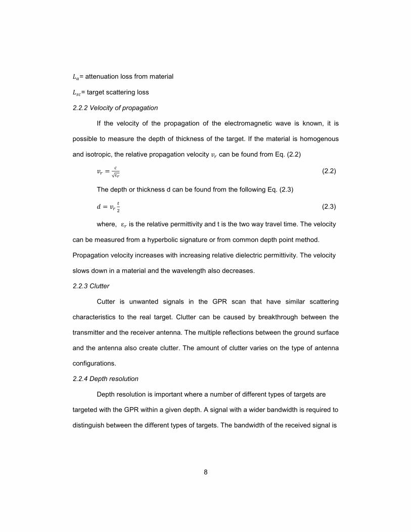
3.1 GPR Theory
GPR is a non-destructive electromagnetic technique that is used to investigate
the features buried under ground. The operating principal of GPR is similar to
conventional radar but it is used in opaque medium such as ground, concrete etc. The
propagation of GPR wave into a medium is governed by Maxwell’s equations. GPR
system normally works using a control unit and a transmitting and receiving antenna. The
transmitter sends signal into the ground. The transmitting signal gets reflected from the
target and the reflected signal is received by the receiver antenna. The received data is
then processed and displayed. A typical GPR system is shown in Fig. 3.1. GPR wave
gets reflected if there is a new material in the path of propagation of the wave. The
reflection wave is the function of the permittivity (ε), the magnetic permeability (μ) and the
electrical conductivity (σ) of the reflection surface (Bostanudin, 2013). A medium with
high conductivity reduces the penetration of the GPR wave because it absorbs the radar
signal. The magnetic permeability is very low for most of the engineering materials. GPR
signal is most susceptible to the permittivity of the medium.
TX RX
Material-2
Material-1
Figure 3-1 Schematic diagram of generic GPR system

12
When GPR wave encounters a change in the manganite of permittivity in its path
of propagation, the following things happen. First, some part of the signal gets absorbed
at the surface. Second, some part of the signal travels through the new surface. Third,
the remaining part of the signal reflected from the surface. This reflected signal is
recorded by the receiver antenna of the GPR system. The amplitude and wavelength
and the travel time of the signal is recorded by GPR. This recorded information consists
of valuable information about the reflection surface or target.
3.1.1 GPR Data Collection
The data collection of GPR on soil or concrete can be done in two different
methods depending on antenna position. If the antenna is in contact with the ground or
concrete surface, then it is called a ground coupled antenna. If the antenna is positioned
at a distance away from the ground, then it is called air-launched antenna. Figure 3.2
shows ground coupled and air-launched antenna.
(a) Ground coupled (b) Air-launched
Figure 3-2 Ground coupled and air-launched antenna (GSSI Concrete Handbook, 2015)
13
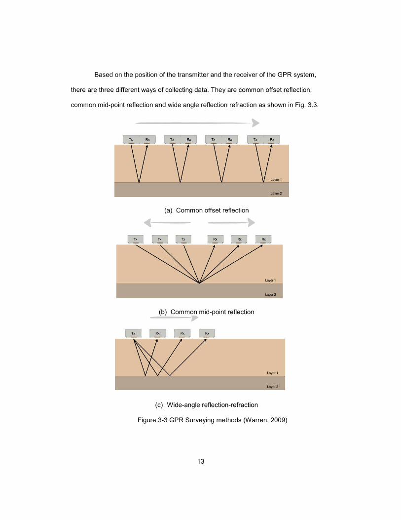
Based on the position of the transmitter and the receiver of the GPR system,
there are three different ways of collecting data. They are common offset reflection,
common mid-point reflection and wide angle reflection refraction as shown in Fig. 3.3.
(a) Common offset reflection
(b) Common mid-point reflection
(c) Wide-angle reflection-refraction
Figure 3-3 GPR Surveying methods (Warren, 2009)

14
In common offset method, the antenna travels over the surface to perform a scan
and the distance between the transmitter and receiver is constant. The transmitter and
the receiver both moves together during a scan. In common midpoint method, a particular
point in the subsurface is targeted. The transmitter and the receiver move away from
each other at a constant rate. In wide-angle reflection-refraction method, the transmitter
is stationary but the position of the receiver is varied and data is collected from each of
the positions of the receiver. In this study, the common offset method was used to collect
the data.
Data collection can be classified based on the orientation of the antenna as well.
Normally in an antenna, the transmitter is positioned at the front and the receiver is
positioned at the back. When the transmitter and the receiver are along the line of the
scan, then it is called normal orientation of the antenna. When the transmitter and
receiver are perpendicular to the direction of scan, then it is called cross-polarized
orientation of the antenna. Figure 3.4 shows the normal and cross polarized antenna.
Figure 3-4 Antenna polarization (GSSI Concrete Handbook, 2015)

15
3.1.2 Property of the medium
The propagation of the electromagnetic wave through a medium depends on the
electromagnetic constitutive properties of the medium. The constitutive properties are
electrical conductivity, magnetic permeability and electrical permittivity. A medium that
has high electrical conductivity such as clay attenuates the GPR signal. Presence of
water also increases the conductivity and creates absorption of energy from the signal.
The most important material property that controls the speed of radar wave is the
permittivity of the medium. The ratio of the permittivity of a material to the permittivity of
free space is called the dielectric constant of the material. The higher the dielectric
constant of a material, the slower the speed of radar wave through it. If the dielectric
constant of a material is known, the depth of the target can be measured. Radar wave
travels faster in materials having low dielectric constant. Therefore, to produce a better
GPR scan, a low dielectric medium is expected. Table 3.1 show the dielectric constant of
some common materials.
Table 3-1 Dielectric constant of common materials (Warren, 2009)
Materials εr
Air 1
Clay (dry) 2-20
clay (wet) 15-40
Concrete (dry) 4-10
Concrete (wet) 10-20
Fresh Water 81
Fresh water ice 3-4
Granite (dry) 5-8
Granite (wet) 5-15
Limestone (dry) 4-8
Limestone (wet) 6-15
Sand (dry) 4-6
Sand (wet) 10-30
Soil (average) 16
Iron Oxides 14

16
3.1.3 GPR Scan output
The output signal of GPR scan possesses valuable information about the
subsurface. The output of the GPR scan is not the real image of the subsurface. Rather it
is a type of signature depends on the size, shape and dielectric constant of the target.
The first reflection of the GPR wave is called direct wave or direct coupling. This direct
wave indicates the top surface. Figure 3.5 shows a GPR reflection signal with direct
coupling at the top of it.
Figure 3-5 Direct coupling or direct wave form the surface (GSSI Concrete Handbook, 2015)
GPR scan data can be collected and presented in one, two and three dimensions
as discussed below.
(1) A-Scan
An A-Scan is a one dimensional scan where the travel time of the GPR wave is
in the x-axis and the amplitude of the reflection is in the y-axis. The transmitter and the
receiver are both kept to an stationary position. A-Scan is also called line-scan or
oscilloscope scan. Figure 3.6 shows an A-Scan.

17
Figure 3-6 GPR A-Scan
(2) B-scan
GPR B-scan is a two dimensional image of the subsurface. When the antenna is
moved on the surface, series of A-Scans are recorded by GPR. By combining all the A-
Scans side by side, the B-scan is produced. Most GPR scanning is done to produce a B-
scan. B-Scans are sometimes called radargram. Figure 3.7 shows a B-scan with a A-
Scan on the right. The x-axis can be distance or number of A-Scans and the y-axis is
time.
Figure 3-7 GPR B-Scan or radargram
-1,500
-1,000
-500
0
500
1,000
1,500
0.00 1.00 2.00 3.00 4.00 5.00 6.00
Am
pli
tud
e
nanoseconds

18
(3) C-Scan
C-Scan is three dimensional scan. The B-Scans or the radargrams can be
collected in a grid and all the B-Scans can be combined together to produce a 3-D map
of the subsurface . Figure 3.8 shows a C-Scan of concrete slab. The grid of
reinforcement is visible.
Figure 3-8 GPR C-Scan or 3-D view (GSSI Concrete Handbook, 2015)
3.1.4 Horizontal and Depth Resolution
The number of scans per unit length of the survey direction control the horizontal
resolution of the B-Scan or radargram. The vertical penetration depth depends on the
frequency of the antenna. The lower is the frequency, the higher the penetration depth.
Similarly, the higher is the frequency, the lower the penetration depth. But at the same
time, the higher is the frequency, the higher the vertical resolution of the B-Scan. So,
selecting an appropriate antenna is very important depending on the type of investigation.
19
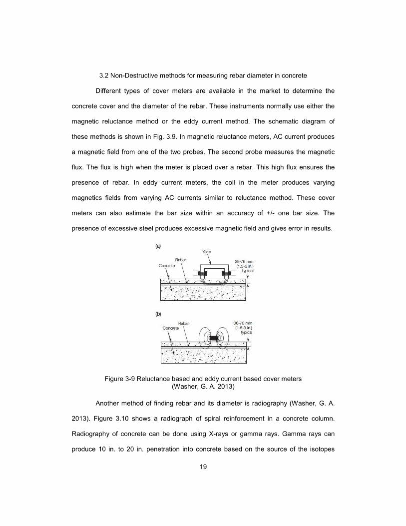
3.2 Non-Destructive methods for measuring rebar diameter in concrete
Different types of cover meters are available in the market to determine the
concrete cover and the diameter of the rebar. These instruments normally use either the
magnetic reluctance method or the eddy current method. The schematic diagram of
these methods is shown in Fig. 3.9. In magnetic reluctance meters, AC current produces
a magnetic field from one of the two probes. The second probe measures the magnetic
flux. The flux is high when the meter is placed over a rebar. This high flux ensures the
presence of rebar. In eddy current meters, the coil in the meter produces varying
magnetics fields from varying AC currents similar to reluctance method. These cover
meters can also estimate the bar size within an accuracy of +/- one bar size. The
presence of excessive steel produces excessive magnetic field and gives error in results.
Figure 3-9 Reluctance based and eddy current based cover meters (Washer, G. A. 2013)
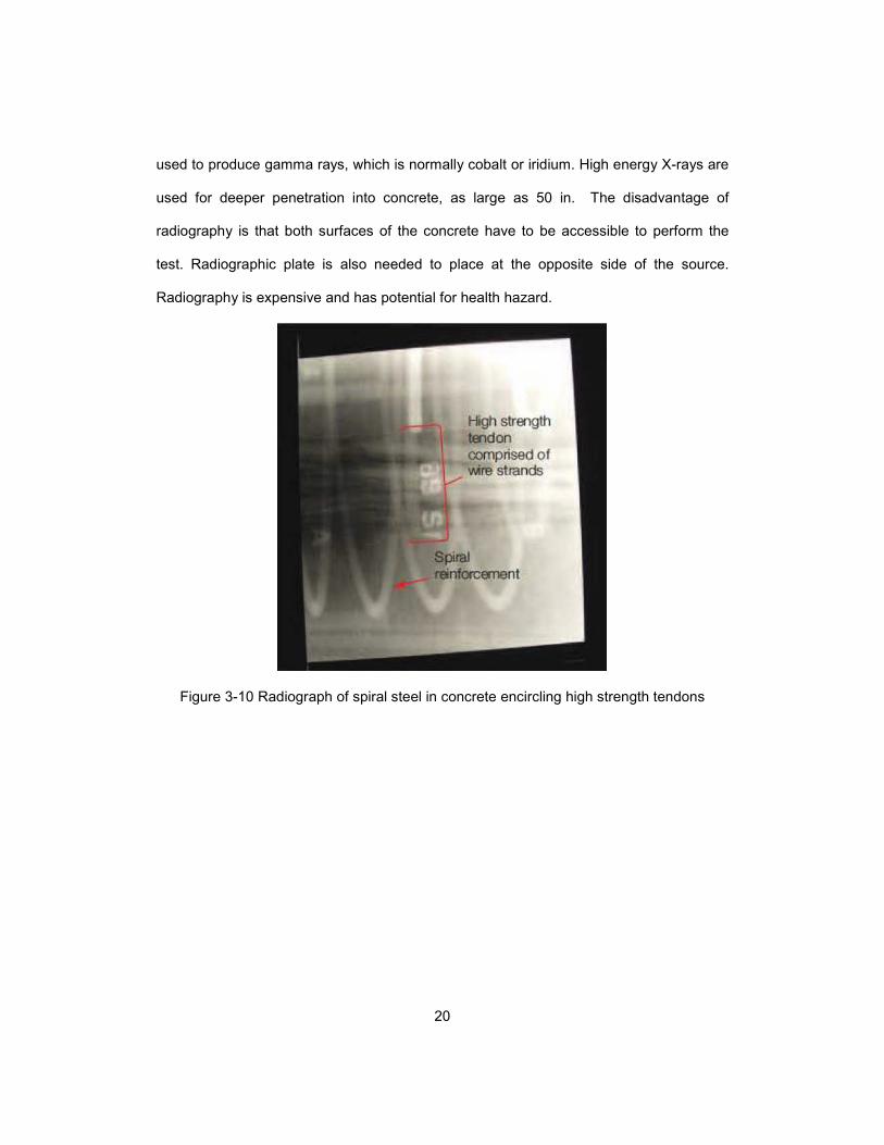
Another method of finding rebar and its diameter is radiography (Washer, G. A.
2013). Figure 3.10 shows a radiograph of spiral reinforcement in a concrete column.
Radiography of concrete can be done using X-rays or gamma rays. Gamma rays can
produce 10 in. to 20 in. penetration into concrete based on the source of the isotopes
20
used to produce gamma rays, which is normally cobalt or iridium. High energy X-rays are
used for deeper penetration into concrete, as large as 50 in. The disadvantage of
radiography is that both surfaces of the concrete have to be accessible to perform the
test. Radiographic plate is also needed to place at the opposite side of the source.
Radiography is expensive and has potential for health hazard.
Figure 3-10 Radiograph of spiral steel in concrete encircling high strength tendons
21
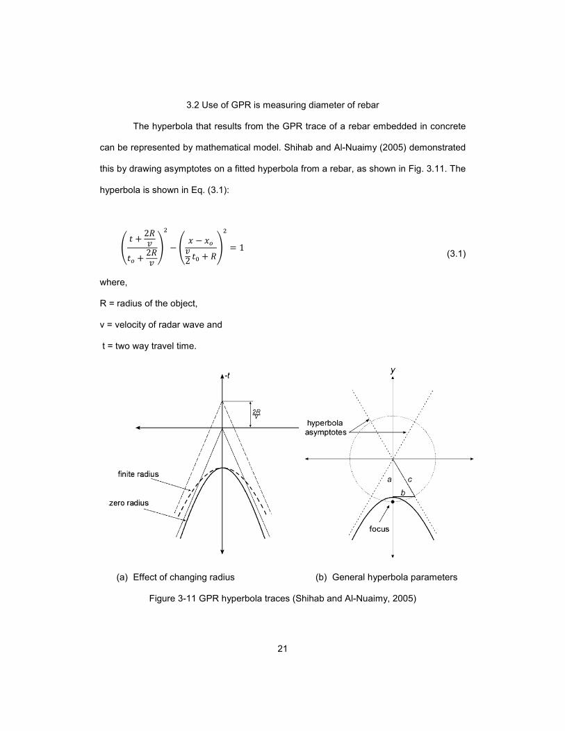
3.2 Use of GPR is measuring diameter of rebar
The hyperbola that results from the GPR trace of a rebar embedded in concrete
can be represented by mathematical model. Shihab and Al-Nuaimy (2005) demonstrated
this by drawing asymptotes on a fitted hyperbola from a rebar, as shown in Fig. 3.11. The
hyperbola is shown in Eq. (3.1):
� � + 2! �" + 2! #
− � $ − $" 2 �% + !#
= 1 where,
R = radius of the object,
v = velocity of radar wave and
t = two way travel time.
(3.1)
(a) Effect of changing radius (b) General hyperbola parameters
Figure 3-11 GPR hyperbola traces (Shihab and Al-Nuaimy, 2005)

22
The radius can be estimated by the following equations (Eq. 3.2 to Eq. 3.5):
' = �" + 2! (3.2)
( = 2 )�" + 2! * (3.3)
= 2(' (3.4)
! = ((' − �%)' (3.5)
where,
a = distance from the tip of hyperbola to surface,
b = distance from the tip of the hyperbola to the asymptotes as in Figure 3.11,
t = two way travel time of radar wave,
v = velocity of radar wave and
R = radius of the object

23
Utsi and Utsi (2004) used 2 GHz and 4 GHz GPR antenna and found the
correlation between the rebar diameter and the maximum amplitude from rebar with two
different antenna orientation. It was shown that the maximum amplitude increased with
the increase of rebar diameter as shown in Fig. 3.12.
Figure 3-12 Relationship between rebar diameter and maximum normal amplitude at different depths (Utsi and Utsi, 2004)
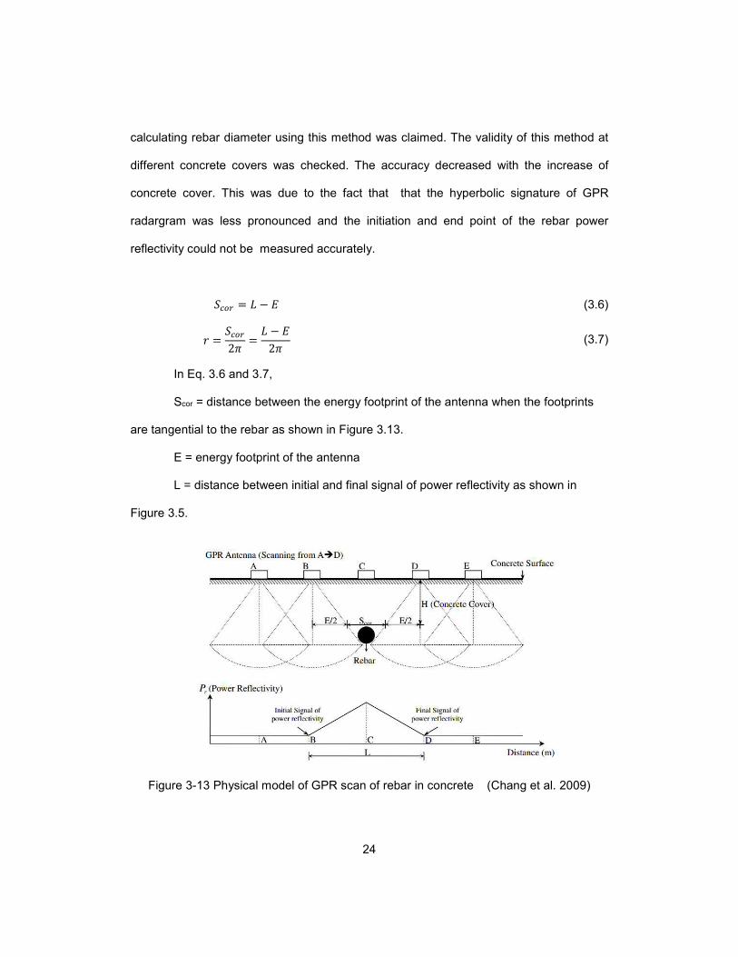
Chang et al. (2009) proposed a physical model of rebar scanning embedded in
concrete with a GPR antenna, as shown in Fig. 3.13. The model considered the radius of
the rebar. The power reflectivity from the rebar was plotted against the distance traveled
by the GPR antenna. The initiation and the end of power reflectivity along the scan
direction were determined from the radargram. The distance between the beginning and
end point of power reflectivity was measured by converting the B-Scan of the image to an
alpha-numeric code using MATLAB. Once the parameters shown in Fig. 3.13 were
determined; the diameter was calculated using Eqs. 2.6 and 2.7. An accuracy of 7% in
0
500
1000
1500
2000
2500
3000
3500
4000
4500
5000
-5 5 15 25 35 45
Am
pli
tud
e
Diameter (mm)
24
calculating rebar diameter using this method was claimed. The validity of this method at
different concrete covers was checked. The accuracy decreased with the increase of
concrete cover. This was due to the fact that that the hyperbolic signature of GPR
radargram was less pronounced and the initiation and end point of the rebar power
reflectivity could not be measured accurately.
-�"� = � − . (3.6)
/ = -�"�20 = � − .20 (3.7)
In Eq. 3.6 and 3.7,
Scor = distance between the energy footprint of the antenna when the footprints
are tangential to the rebar as shown in Figure 3.13.
E = energy footprint of the antenna
L = distance between initial and final signal of power reflectivity as shown in
Figure 3.5.
Figure 3-13 Physical model of GPR scan of rebar in concrete (Chang et al. 2009)

25
Leucci, G. (2012) used two different antenna orientations to scan the rebar in
concrete, as shown in Fig. 3.14. First, the transmitter and receiver of the antenna were
perpendicular to the rebar during the scan, and second, the antennae were rotated by 90
degrees so that the transmitter and receiver became parallel to the rebar during the GPR
scan. It was shown that the perpendicular orientation gave a stronger amplitude response
than the parallel orientation of the rebar. A correlation of the ratio of maximum amplitude
from the rebar in both antenna orientations was tried, with the diameter of the rebar as
shown in Fig. 3.15.
Figure 3-14 Antenna orientations: (a) co-polarized; (b) cross-polarized (Leucci, G. 2012)
(a) (b)

26
Figure 3-15 Correlation between bar diameter and amplitude ratio (Leucci, G. 2012)
Zanzi and Arosio (2013) used the concept of Radar Cross Section (RCS) of the
rebar. RCS is a quantity which indicates the relation between amount of energy going to
a target form the GPR antenna and the reflected energy from the antenna. This study
showed that the ratio of RCS in co-polar and cross polar direction was related with the
rebar diameter. But sensitivity and accuracy of the method was dependent on the
frequency of the antenna. It was demonstrated that RCS ratio of different rebar
diameters had different sensitive zones based on the frequency of the antenna used in
scanning (Fig. 3.16). A finite difference time domain (FDTD) model was established to
compare the test results with theoretical results. Figure 3.16 shows that for smaller
diameter of rebar, the higher antenna frequency found a steady relation between RCS
0
2
4
6
8
10
12
14
16
18
20
22
24
26
28
30
32
0 0.2 0.4 0.6 0.8 1 1.2 1.4 1.6
Ba
r D
iam
ete
r (m
m)
Amplitude Ratio (Ar)
d = 4.482Ar4.7241
R=0.8873

27
ratio and diameter. As the diameter of the rebar increased, the lower frequency antenna
was steady but the higher frequency RCS ratios started fluctuating.
Figure 3-16 RCS ratio for three different antenna frequencies (Zanzi and Arosio, 2013)
3.3 Corrosion Background
Corrosion happens when the passive film on the rebar surface in reinforced
concrete breaks down mostly by chloride ions (Bertolini el al., 1996). Corrosion is an
electrochemical process and electrochemical galvanic cell forms in concrete during
corrosion process. The rebars in concrete acts as anode and also as cathode. The pore
water in concrete acts as an aqueous medium and carries the chloride ions to the rebar.
The pH level of concrete surrounding the rebar is very high (12 to 13) due to the
presence of alkaline oxides as Ca(OH)2 . Due to carbonation of concrete or ingress of
chloride ions, the pH level goes down close to 7 and the anodic and catholic reactions of
corrosion initiates. The following possible anodic reactions (Eq. 3.8 t0 Eq. 3.13) can
happen based on the pH of concrete, presence of aggressive anions, and presence of
adequate electrical potentials at the vicinity of steel surface (Ahmad, 2003).
28
3Fe + 4H2O → Fe3O4 + 8H+ + 8e- (3.8)
2Fe + 3H2O → Fe2O3 + 6H+ + 6e- (3.9)
Fe + 2H2O → HFeO2- + 3H+ + 2e- (3.10)
Fe → Fe2+ + 2e- (3.11)
The following are the possible cathodic reactions
2H2O + O2 +4e- → 4OH- (3.12)
2H+ + 2e- →H2 (3.13)
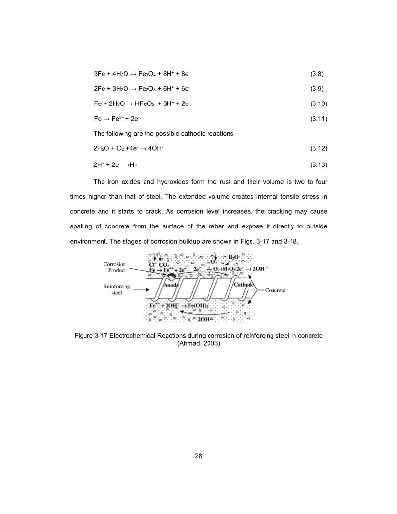
The iron oxides and hydroxides form the rust and their volume is two to four
times higher than that of steel. The extended volume creates internal tensile stress in
concrete and it starts to crack. As corrosion level increases, the cracking may cause
spalling of concrete from the surface of the rebar and expose it directly to outside
environment. The stages of corrosion buildup are shown in Figs. 3-17 and 3-18.
Figure 3-17 Electrochemical Reactions during corrosion of reinforcing steel in concrete (Ahmad, 2003)

29
Before Corrosion Build-up of
Corrosion Products
Further Corrosion, Surface Cracks,
Stains.
Eventual Spalling, Corroded
Bar,Exposed.
Figure 3-18 Corrosion of steel reinforcement in concrete (The Helpful Engineer, 2010)
The detection of concrete corrosion is very important for the repair and
maintenance of an existing structure. It is also important for the strength evaluation and
service life prediction of an existing structure. The testing method is desired to be non-
destructive in order to ensure minimum physical damage and minimum disruption of
service. The purpose of corrosion testing is to determine the presence of corrosion
process and also the intensity and rate of corrosion damage. Three main methods of
non-destructive evaluation (NDE) of concrete corrosion are currently available: half-cell
potential method, concrete resistivity method and the linear polarization resistance
method.
3.3.1 Half Cell Potential Method (ASTM C876-09, 2014)
The corrosion potential of the steel can be measured from the surface of the
concrete using a standard half-cell. The measured potential indicates the portability of
corrosion at the point of measurement. No quantitative information can be obtained by
this method as the output is probability based. The schematic diagram of the half-cell
potential method is shown in Fig. 3.19. This method is not totally non-destructive because
it needs at least one rebar to be physically exposed for direct electrical connection.
30
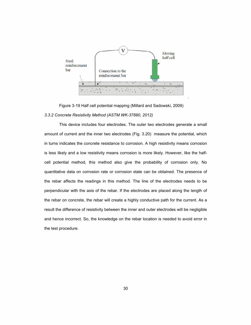
Figure 3-19 Half cell potential mapping (Millard and Sadowski, 2009)
3.3.2 Concrete Resistivity Method (ASTM WK-37880, 2012)
This device includes four electrodes. The outer two electrodes generate a small
amount of current and the inner two electrodes (Fig. 3.20) measure the potential, which
in turns indicates the concrete resistance to corrosion. A high resistivity means corrosion
is less likely and a low resistivity means corrosion is more likely. However, like the half-
cell potential method, this method also give the probability of corrosion only. No
quantitative data on corrosion rate or corrosion state can be obtained. The presence of
the rebar affects the readings in this method. The line of the electrodes needs to be
perpendicular with the axis of the rebar. If the electrodes are placed along the length of
the rebar on concrete, the rebar will create a highly conductive path for the current. As a
result the difference of resistivity between the inner and outer electrodes will be negligible
and hence incorrect. So, the knowledge on the rebar location is needed to avoid error in
the test procedure.
31
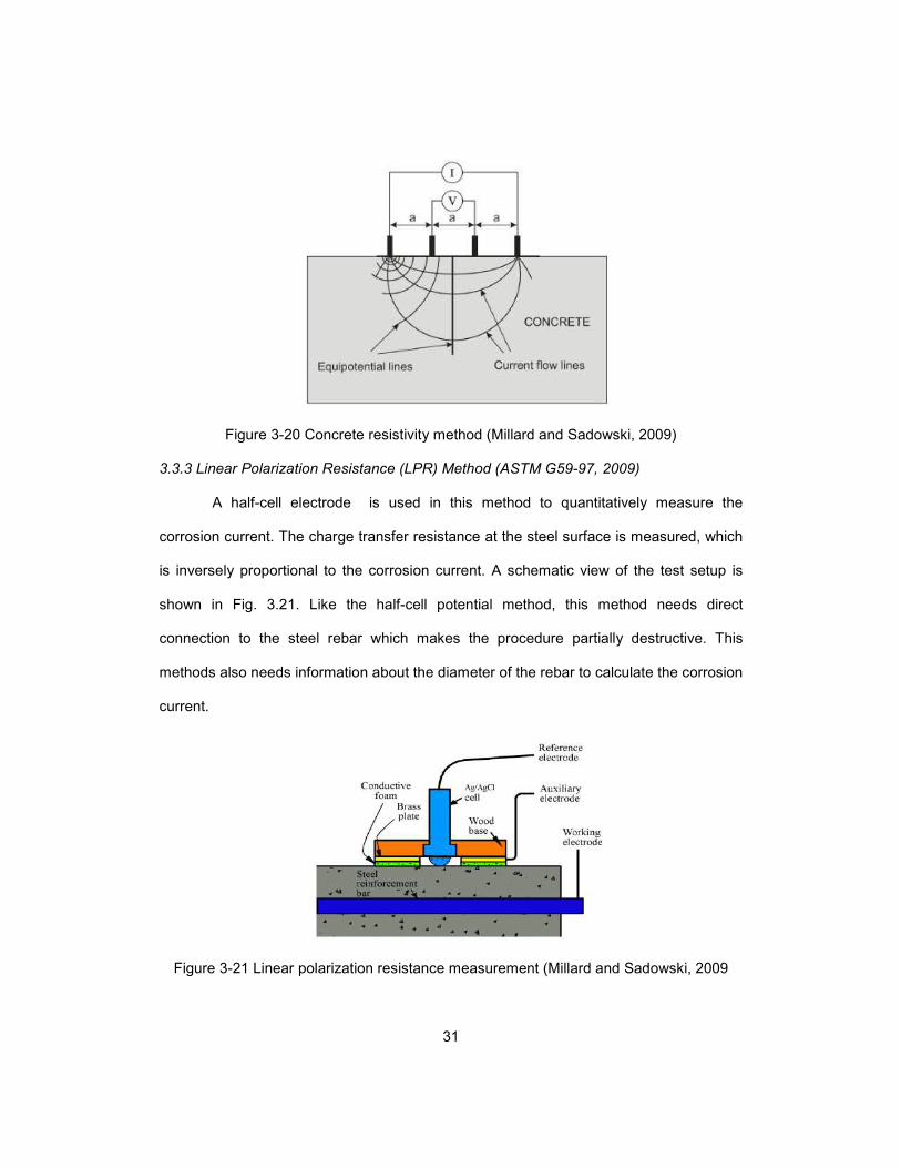
Figure 3-20 Concrete resistivity method (Millard and Sadowski, 2009)
3.3.3 Linear Polarization Resistance (LPR) Method (ASTM G59-97, 2009)
A half-cell electrode is used in this method to quantitatively measure the
corrosion current. The charge transfer resistance at the steel surface is measured, which
is inversely proportional to the corrosion current. A schematic view of the test setup is
shown in Fig. 3.21. Like the half-cell potential method, this method needs direct
connection to the steel rebar which makes the procedure partially destructive. This
methods also needs information about the diameter of the rebar to calculate the corrosion
current.
Figure 3-21 Linear polarization resistance measurement (Millard and Sadowski, 2009
32
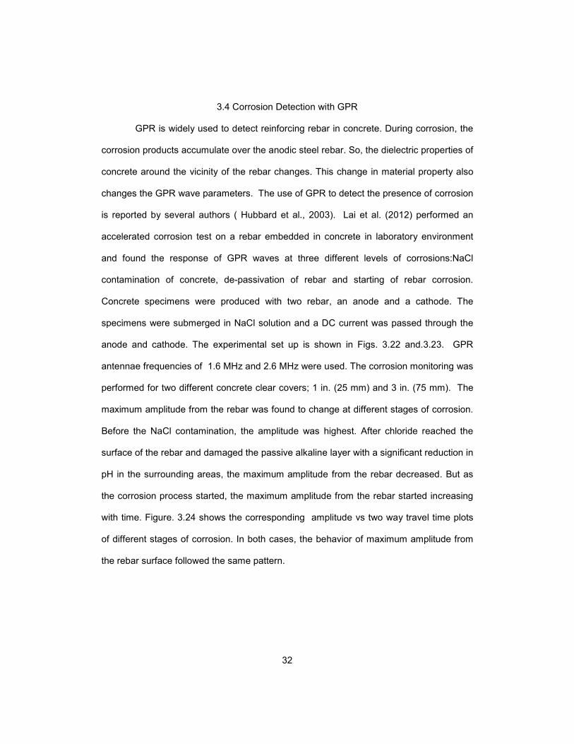
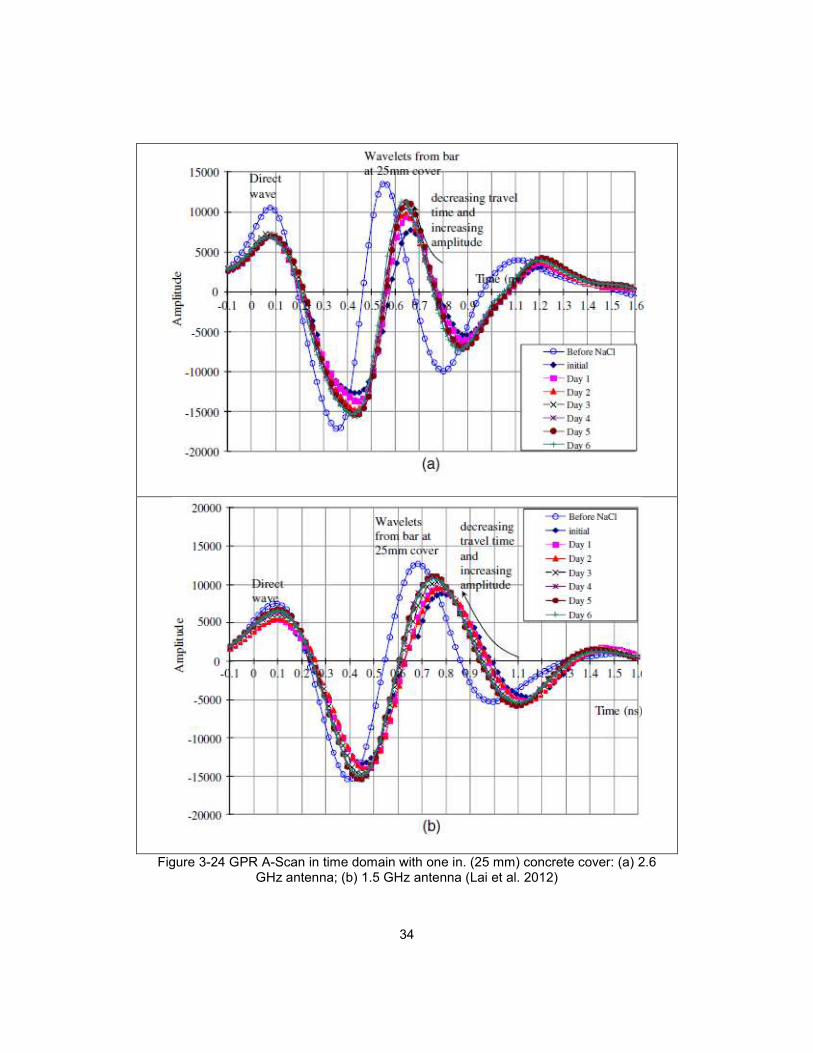
3.4 Corrosion Detection with GPR
GPR is widely used to detect reinforcing rebar in concrete. During corrosion, the
corrosion products accumulate over the anodic steel rebar. So, the dielectric properties of
concrete around the vicinity of the rebar changes. This change in material property also
changes the GPR wave parameters. The use of GPR to detect the presence of corrosion
is reported by several authors ( Hubbard et al., 2003). Lai et al. (2012) performed an
accelerated corrosion test on a rebar embedded in concrete in laboratory environment
and found the response of GPR waves at three different levels of corrosions:NaCl
contamination of concrete, de-passivation of rebar and starting of rebar corrosion.
Concrete specimens were produced with two rebar, an anode and a cathode. The
specimens were submerged in NaCl solution and a DC current was passed through the
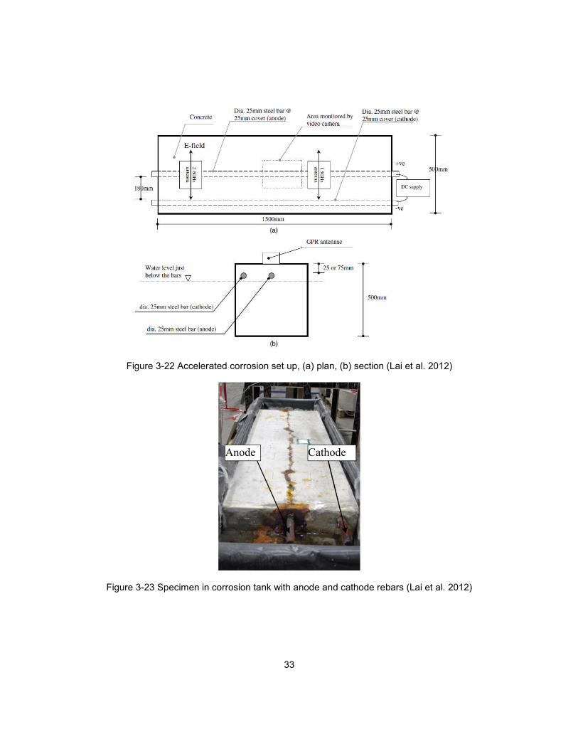
anode and cathode. The experimental set up is shown in Figs. 3.22 and.3.23. GPR
antennae frequencies of 1.6 MHz and 2.6 MHz were used. The corrosion monitoring was
performed for two different concrete clear covers; 1 in. (25 mm) and 3 in. (75 mm). The
maximum amplitude from the rebar was found to change at different stages of corrosion.
Before the NaCl contamination, the amplitude was highest. After chloride reached the
surface of the rebar and damaged the passive alkaline layer with a significant reduction in
pH in the surrounding areas, the maximum amplitude from the rebar decreased. But as
the corrosion process started, the maximum amplitude from the rebar started increasing
with time. Figure. 3.24 shows the corresponding amplitude vs two way travel time plots
of different stages of corrosion. In both cases, the behavior of maximum amplitude from
the rebar surface followed the same pattern.
33
Figure 3-22 Accelerated corrosion set up, (a) plan, (b) section (Lai et al. 2012)
Figure 3-23 Specimen in corrosion tank with anode and cathode rebars (Lai et al. 2012)
Anode Cathode
34
Figure 3-24 GPR A-Scan in time domain with one in. (25 mm) concrete cover: (a) 2.6 GHz antenna; (b) 1.5 GHz antenna (Lai et al. 2012)

35
Lai et al. (2012) also plotted the increase in amplitude from the rebar with the
progress of corrosion time, as shown in Fig 3.25.
Figure 3-25 Increase in rebar amplitude with time (Lai et al., 2012)
Hong et al. (2014) performed a similar study on accelerated corrosion. The peak
to peal amplitude of the direct wave (DW) and the reflected wave (RW) were taken as
GPR parameters, as shown in Fig. 3.26. The change of peak to peak amplitude of DW
and RW was monitored with the progress of corrosion in the specimen. It was observed
that the peak to peak amplitude was increased with time, as shown in Fig. 3.27. As
shown in Fig. 3.27, the changes in amplitude in anode rebar were found to be more
prominent than in the cathode rebar. This is reasonable because all the corrosion
products accumulated around the anode.

36
.
Figure 3-26 DW, RW and peak to peak amplitude (Hong et al., 2014)
Figure 3-27 Changes in peak to peak amplitude for RW from rebar (Hong et al., 2014)
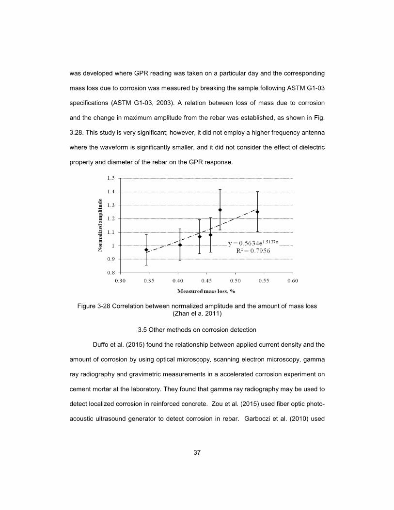
Zhan et al. (2011) performed accelerated corrosion testing using a one GHz
antenna and 20 mm (0.80 in.) diameter steel rebar embedded in concrete. A test matrix
Pea
k t
o p
eak A
mp
.
37
was developed where GPR reading was taken on a particular day and the corresponding
mass loss due to corrosion was measured by breaking the sample following ASTM G1-03
specifications (ASTM G1-03, 2003). A relation between loss of mass due to corrosion
and the change in maximum amplitude from the rebar was established, as shown in Fig.
3.28. This study is very significant; however, it did not employ a higher frequency antenna
where the waveform is significantly smaller, and it did not consider the effect of dielectric
property and diameter of the rebar on the GPR response.
Figure 3-28 Correlation between normalized amplitude and the amount of mass loss (Zhan el a. 2011)
3.5 Other methods on corrosion detection
Duffo et al. (2015) found the relationship between applied current density and the
amount of corrosion by using optical microscopy, scanning electron microscopy, gamma
ray radiography and gravimetric measurements in a accelerated corrosion experiment on
cement mortar at the laboratory. They found that gamma ray radiography may be used to
detect localized corrosion in reinforced concrete. Zou et al. (2015) used fiber optic photo-
acoustic ultrasound generator to detect corrosion in rebar. Garboczi et al. (2010) used

38
electromagnetic wave on the order of 100 GHz or higher to detect two different types of
corrosion product on the surface of the rebar.
Kim et al. (2011) used four different types of corrosion products and tested their
permittivity and magnetic permeability with increasing frequency of the electromagnetic
wave ranging from 1 GHz to 6 GHz. Figure 3.29 shows the change in dielectric
permittivity of different corrosion products with increasing frequency. It was observed that
the dielectric permittivity of the corrosion products do not significantly change with
frequency.
(a) (b)
Figure 3-29 Change of dielectric permittivity ɛ′ (a) and ɛ″ (b) of different corrosion product with increasing frequency (Kim et al., 2010)
Figure 3.29 shows the change in magnetic permeability of different corrosion
products with increasing frequency. It was observed that the magnetic permeability of the
corrosion products significantly change with frequency especially in the range of 0 to 2
GHz. This change can be used to detect the presence of corrosion in the rebar.
39
(a) (b)
Figure 3-30 Change of magnetic permeability μ′ (a) and μ″ (b) of different corrosion product with increasing frequency (Kim et al., 2010)
3.6 Limitation of previous study and significance of the research
Corrosion of rebar in concrete is the one of the most significant reasons that is
responsible for the reduction of design service life of the structure. Corrosion process
reduces the effective area of the rebar and results in reduction of design strength of the
structural component. Early detection of corrosion can significantly reduce the repair cost.
When corrosion appears visually on the surface on the concrete, then it is very difficult to
avoid expensive and time consuming repair scheme. Currently there is no NDT method
that can provide quantitative data on corrosion. Using GPR to investigate quantitative
data on corrosion will be an excellent addition to the existing usage of GPR.
In order to determine the loss of rebar area due to corrosion, it is needed to
measure the reduced area of the rebar. Existing NDT methods of measuring the rebar
size are not accurate enough to detect the corrosion induced change in rebar area.
Existing NDT methods to detect corrosion such as half-cell potential, concrete resistivity
and linear polarization can not give quantitative information on corrosion. Though GPR

40
has been used to detect the presence of corrosion, it has not been used to quantify loss
of area or mass due to corrosion.
Currently GPR is used extensively to locate rebar and detect deteriorated area of
concrete especially on a bridge deck. The same data for locating rebar and detecting
concrete deterioration can be used to perform the quantitative measurement of corrosion
in concrete. If done so, significant amount of time and resources can be saved. Collecting
data using GPR is much quicker than any existing method of detecting corrosion such as
half-cell potential. GPR is also totally non-destructive whereas half-cell potential is
partially destructive.
In this research a higher frequency GPR antenna was used which is not used
previously to study the quantitative measurement of corrosion. No study is done so far to
relate the GPR parameters to actual physical loss of mass of rebar. A novel approach to
use in oil-emulsion tank with submerged rebar as a substitute of actual reinforced
concrete is used in this study. Existing studies to detect corrosion using GPR do not
consider the effect of dielectric permittivity of the medium. In this study, the effect of
dielectric permittivity on corrosion data of GPR is addressed. Finally a method is
proposed to determine the amount of corrosion using GPR.
41
Chapter 4
Effect of various GPR parameters on rebar diameter estimation
4.1 Introduction
In this chapter the effect of various GPR parameters on the diameter of rebar in
concrete are tested and the results are discussed. The size of the rebar was estimated
based on the GPR parameters. The size of the rebar or rebar diameter is a function of
number of GPR parameters and number of physical parameters associated with the
rebar. Currently there are no well-established methods to determine the diameter of rebar
using GPR with expected degree of accuracy. In this phase of the study, six different
diameters of rebar were used to make the concrete beam sample. Concrete beam
specimens were cast and subsequently scanned by GPR. The GPR readings were then
taken into post-processing software called RADAN (RADAN 7, 2014). Basic post
processing of raw GPR data were done using RADAN and the important parameters
related to rebar diameter were retrieved from the processed data. The parameters were
plotted against rebar diameter and discussions were made on the observed results. The
GPR scans and the parameters were used to estimate the rebar diameter and the
accuracy of the methods were discussed.
4.2 Materials and Equipment Used
Commercially available deformed steel rebars were used in this study. The
concrete beams were made of plain concrete with no admixtures with ordinary Portland
cement. The GPR system was acquired from Geophysical Survey System Inc. (GSSI).
4.2.1 Rebars
Six different diameters of rebars were selected for the study. The diameters were
ranging from #3 (10 mm) to #11 (36 mm) as showed in the following Table 4.1. Figure 4.1
shows the different diameter of rebars that were used in this study before casting them
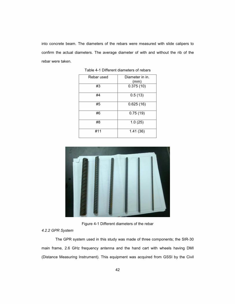
42
into concrete beam. The diameters of the rebars were measured with slide calipers to
confirm the actual diameters. The average diameter of with and without the rib of the
rebar were taken.
Table 4-1 Different diameters of rebars
Rebar used Diameter in in. (mm)
#3 0.375 (10)
#4 0.5 (13)
#5 0.625 (16)
#6 0.75 (19)
#8 1.0 (25)
#11 1.41 (36)
Figure 4-1 Different diameters of the rebar
4.2.2 GPR System
The GPR system used in this study was made of three components; the SIR-30
main frame, 2.6 GHz frequency antenna and the hand cart with wheels having DMI
(Distance Measuring Instrument). This equipment was acquired from GSSI by the Civil
43
Engineering Department of UT Arlington. The SIR-30 main frame was made of radar
boards and operating computer to generate the radar wave through its channels. The
SIR-30 had four channels for antenna output which means four antennas can be
connected with it at a time. The SIR-30 was able to generate a wide range of frequencies
depending on the antenna connected to it. The frequency of the antenna used in this
study was 2.6 GHz. This was the highest frequency that was commercially available in
the GPR industry. As per GPR theory, the resolution of a GPR subsurface image is
proportional to the magnitude of the frequency of the antenna. So this antenna was
supposed to give the best resolution of GPR image for our study. The penetration depth
of this antenna was 1 ft. (0.3 m) which was adequate because most rebars normally
locate within a few inches from the surface of the concrete. The antenna was attached
with the hand cart which can measure distance. The SIR-30 can simultaneously collect
the scan form the antenna and the distance reading from the cart wheels. A total GPR
system is shown the following Fig. 4.2.
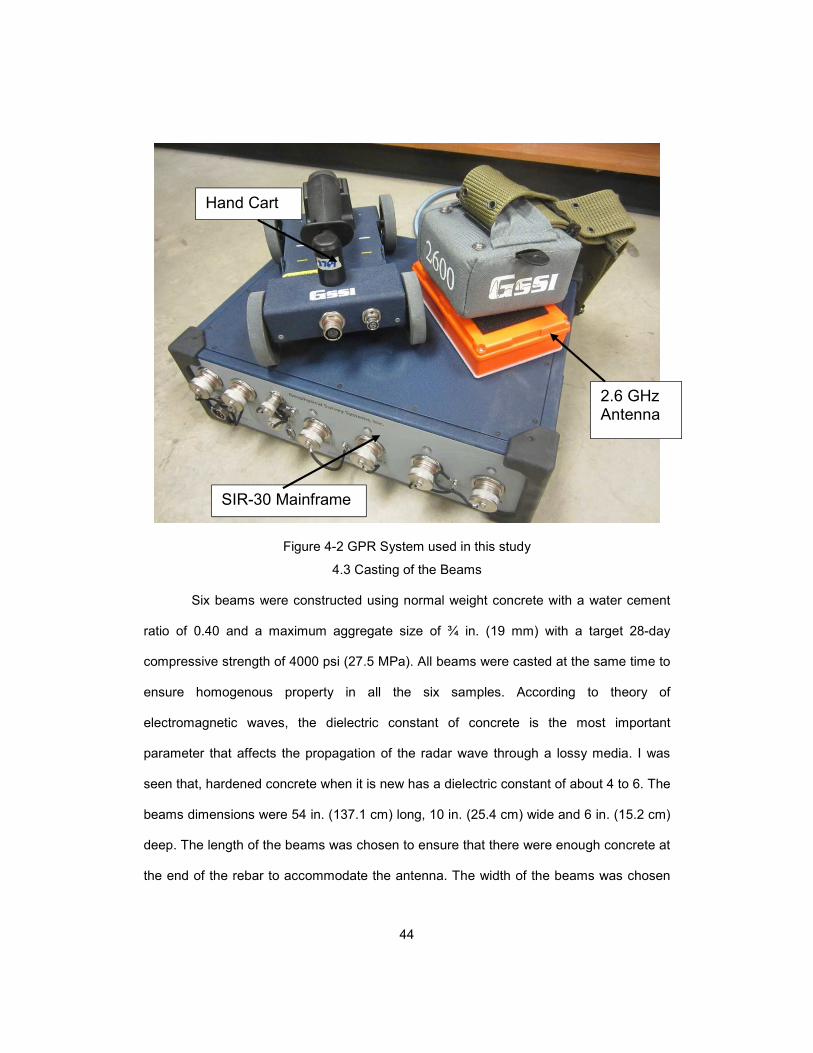
44
Figure 4-2 GPR System used in this study
4.3 Casting of the Beams
Six beams were constructed using normal weight concrete with a water cement
ratio of 0.40 and a maximum aggregate size of ¾ in. (19 mm) with a target 28-day
compressive strength of 4000 psi (27.5 MPa). All beams were casted at the same time to
ensure homogenous property in all the six samples. According to theory of
electromagnetic waves, the dielectric constant of concrete is the most important
parameter that affects the propagation of the radar wave through a lossy media. I was
seen that, hardened concrete when it is new has a dielectric constant of about 4 to 6. The
beams dimensions were 54 in. (137.1 cm) long, 10 in. (25.4 cm) wide and 6 in. (15.2 cm)
deep. The length of the beams was chosen to ensure that there were enough concrete at
the end of the rebar to accommodate the antenna. The width of the beams was chosen
Hand Cart
SIR-30 Mainframe
2.6 GHz Antenna

45
as 10 in. (25.4 cm) which is enough to accommodate the wheels of the hand cart for the
scanning. The depths of the specimens were 6 in. (15.2) so that the antenna could reach
the bottom of the beam to indicate it in the scan output. The spacing of the rebar was 15
in. (38.1 cm) so that the GPR response from one rebar would not interfere with the GPR
response of and adjacent rebar. Three different concrete covers were used [1 in. (25
mm), 2 in. (50 mm) and 3 in. (75 mm)] in the beams to see the variation of GPR
response with the depth of rebar in concrete. A schematic diagram of the concrete beam
sample is shown in Fig. 4.3.
The
The concrete were mixed according to the mix design. After the mix was ready,
the concrete was immediately poured into the forms as shown in Fig. 4.4. After the
casting was done, the beams were placed in a 100% humidity chamber for 28 days to
finish the hydration process and to get ready for scanning with the GPR.
1″ Cover
15″ 15″ 54″
6″ 2″ Cover 3″ Cover
Figure 4-3 Schematic diagram of the beam specimen
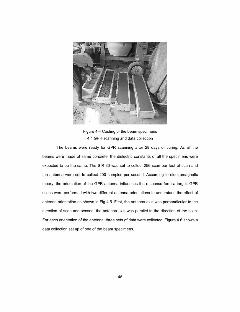
46
Figure 4-4 Casting of the beam specimens
4.4 GPR scanning and data collection
The beams were ready for GPR scanning after 28 days of curing. As all the
beams were made of same concrete, the dielectric constants of all the specimens were
expected to be the same. The SIR-30 was set to collect 256 scan per foot of scan and
the antenna were set to collect 200 samples per second. According to electromagnetic
theory, the orientation of the GPR antenna influences the response form a target. GPR
scans were performed with two different antenna orientations to understand the effect of
antenna orientation as shown in Fig 4.5. First, the antenna axis was perpendicular to the
direction of scan and second, the antenna axis was parallel to the direction of the scan.
For each orientation of the antenna, three sets of data were collected. Figure 4.6 shows a
data collection set up of one of the beam specimens.

47
(a) (b)
Figure 4-5 Antenna orientation, (a) Normal, (b) Parallel
Figure 4-6 GPR scanning of beam specimen with #8 (25 mm) diameter rebar
The radargram data that was collected from different rebar diameters are
presented in Fig. 4.7.

48
(a) GPR scan of #3 (10 mm) rebar (b) GPR scan of #4 (12 mm) rebar
(c) GPR scan of #5 (16 mm) rebar (d) GPR scan of #6 (19 mm) rebar
(e) GPR scan of #8 (25 mm) rebar (f) GPR scan of #11 (35 mm) rebar
Fig. 4.7 GPR Scan of rebar of different sizes for normal antenna orientation

49
4.5 GPR Data Processing
From the GPR scan of the beams in Fig. 4.7, it was seen that the rebars in the
concrete were showing up as hyperbola. When the diameters were larger, the hyperbolic
signatures from the rebar became brighter. However it was very difficult to differentiate
among these hyperbolas without further processing. To harvest more information, the
collected data were taken into post-processing software RADAN by GSSI. RADAN can
improve the quality of the data as well as it can look into other parameters of GPR scan.
The following three easy steps were performed on the collected data.
a) Time Zero (to locate the top surface of concrete)
b) Background Removal ( to remove noise from the scan background)
c) Applying filter ( to remove further noise form the data)
The time zero correction for ground coupled data was not significant. Because
the antenna was already in contact with ground and the gap between the antenna and
the ground was negligible. Time zero correction is very important step when the data is
collected with an air launched antenna. The GPR data processing using RADAN is
shown is Fig. 4.7. Figure 4.7(a) shows the raw GPR radargram without any processing.
The normalized amplitude of the maximum reflective amplitude of the rebar is also shown
with the radargram. Figure 4.7 (b) shows the data after background removal filter was
applied. Background removal eliminated the noise generated by direct coupling at the
interface of concrete and air. The first peak that is observed near the surface is called
direct coupling. It is shown in Fig. 4.7 (b) that the direct coupling was removed after
background removal filter was applied. The data was further smoothened and the
brightness of parabola was amplified by applying FIR (Finite Impulse Response) filter as
shown in Fig. 4.7 (b)
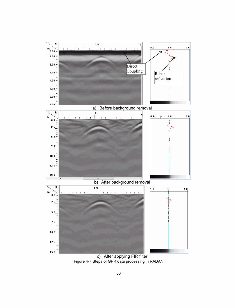
50
a) Before background removal
b) After background removal
c) After applying FIR filter
Figure 4-7 Steps of GPR data processing in RADAN
Direct
Coupling Rebar
reflection

51
Each hyperbolic signature of the GPR data was consisted of many information
about the embedded rebar. When the antenna was not exactly above the rebar, the
amplitude of the reflected signal was smaller. But when the antenna was directly above
the rebar the amplitude of the reflected signal was the maximum. This observation
indicated that the diameter of the rebar was related to the maximum reflected amplitude
of the GPR wave. This maximum amplitude was taken as a main parameter affecting the
size of rebar in concrete in this study. As mentioned previously, each data was taken
three times, therefore the maximum amplitude from a rebar was taken from the average
of three scans for the same beam.
4.6 Effect of maximum amplitude on rebar diameter
The maximum amplitude data were collected from data processing through
RADAN. Table 4.2 shows the collected data from all of beams. These data were plotted
to understand the effect of maximum amplitude on rebar size. The unit of the amplitudes
in the table was GSSI specified data units.

52
Table 4-2 Maximum amplitudes from rebars of different sizes at different depths
Dia Cover Depth
(in.) Normal Amp Polarized Amp
Normal vs Polarized
Ratio
#3
3 141763 497653 0.2848
2 1867737 1014792 1.8405
1 2705771 1697363 1.5941
#4
3 229560 561986 0.4085
2 1940846 1232674 1.5745
1 2715313 1993648 1.3619
#5
3 694691 806327 0.8615
2 1752673 1511943 1.1592
1 2116602 2884789 0.7337
#6
3 226166 791981 0.2855
2 2455797 1634993 1.5020
1 2861853 2569244 1.1138
#8
3 554706 984783 0.5633
2 2635761 2083280 1.2652
1 2496558 3013644 0.8284
#11
3 382871 840632 0.4554
2 2810811 2243191 1.2530
1 3235239 3711821 0.871604261
From radar theory, the ratio of maximum amplitude form two different antenna
orientation can be related to the diameter of the target rebar. The effect of the ratio of
maximum reflected amplitude of two different antenna orientation differed by 90˚ angle, is
discussed in the following section for different concrete covers.

53
4.6.1 Effect of maximum amplitude on rebar diameter
The maximum amplitudes reflected from the rebars of each of the beam
specimens were plotted against the corresponding diameters for different clear cover.
Figure 4.8 showed the variation of maximum amplitude of two different antenna
orientations with the rebar size at a concrete cover depth of 1 in. (25 mm). The amplitude
was increasing with the rebar diameter in both antenna orientation. It was observed that
the amplitudes from polarized orientation of the antenna were more sensitive to change
of diameters as opposed to normal orientation of the antenna.
Figure 4-8 Amplitude vs rebar size at 1 in. (25 mm) cover
Figure 4.9 showed the variation of maximum amplitude of two different antenna
orientations with the rebar size at a concrete cover depth of 2 in (50 mm). The amplitudes
were increasing with the rebar diameters in both antenna orientation. It was observed
that the amplitudes from normal orientation of the antenna were more sensitive to change
of diameters as opposed to polarized orientation of the antenna. The results of amplitude
vs diameter at a concrete cover of 3 in. (75 mm) did not show any consistency. This was
0
2000
4000
6000
8000
10000
12000
14000
0 0.5 1 1.5
Diameter (in.)
1 in. 1 in. Polarized
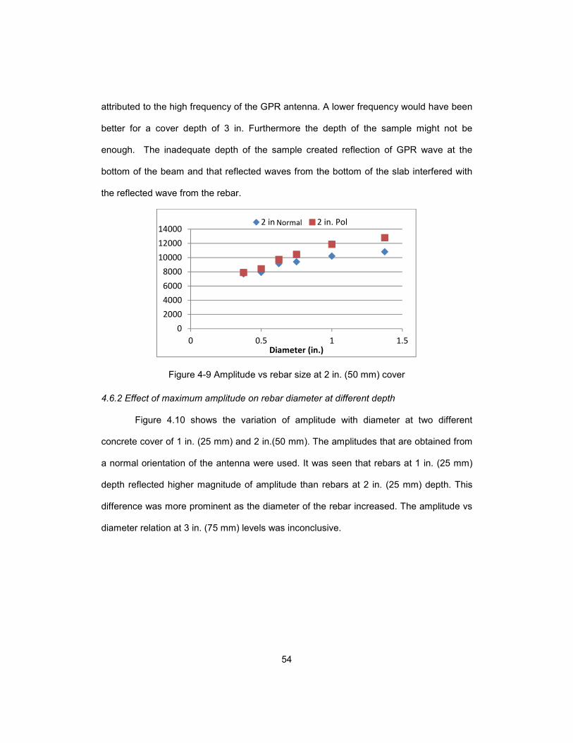
54
attributed to the high frequency of the GPR antenna. A lower frequency would have been
better for a cover depth of 3 in. Furthermore the depth of the sample might not be
enough. The inadequate depth of the sample created reflection of GPR wave at the
bottom of the beam and that reflected waves from the bottom of the slab interfered with
the reflected wave from the rebar.
Figure 4-9 Amplitude vs rebar size at 2 in. (50 mm) cover
4.6.2 Effect of maximum amplitude on rebar diameter at different depth
Figure 4.10 shows the variation of amplitude with diameter at two different
concrete cover of 1 in. (25 mm) and 2 in.(50 mm). The amplitudes that are obtained from
a normal orientation of the antenna were used. It was seen that rebars at 1 in. (25 mm)
depth reflected higher magnitude of amplitude than rebars at 2 in. (25 mm) depth. This
difference was more prominent as the diameter of the rebar increased. The amplitude vs
diameter relation at 3 in. (75 mm) levels was inconclusive.
0
2000
4000
6000
8000
10000
12000
14000
0 0.5 1 1.5Diameter (in.)
2 in 2 in. PolNormal

55
Figure 4-10 Amplitude vs rebar diameter at different depths [1 in. (25 mm), 2 in. (50 mm), and 3 in.(75 mm)]
4.6.3 Effect of maximum amplitude ratio on rebar diameter
The variation of maximum amplitude ratio from two different antenna orientations
is shown in following Fig. 4.11. It was seen that the ratio gradually decreased for rebar
diameter was 1 in. (25 mm) or smaller. The ratio started increasing when the rebar
diameter was greater than 1 in. (25 mm) Therefore, without a prior knowledge about the
diameter, this curve will not be useful to find the relation between diameter and
amplitude.
0
5000
10000
15000
0 0.5 1 1.5
1 2 3in.
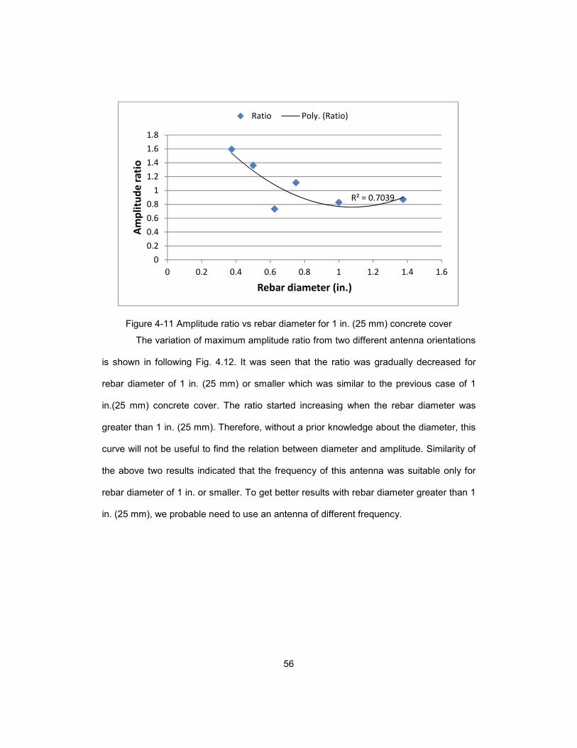
56
Figure 4-11 Amplitude ratio vs rebar diameter for 1 in. (25 mm) concrete cover
The variation of maximum amplitude ratio from two different antenna orientations
is shown in following Fig. 4.12. It was seen that the ratio was gradually decreased for
rebar diameter of 1 in. (25 mm) or smaller which was similar to the previous case of 1
in.(25 mm) concrete cover. The ratio started increasing when the rebar diameter was
greater than 1 in. (25 mm). Therefore, without a prior knowledge about the diameter, this
curve will not be useful to find the relation between diameter and amplitude. Similarity of
the above two results indicated that the frequency of this antenna was suitable only for
rebar diameter of 1 in. or smaller. To get better results with rebar diameter greater than 1
in. (25 mm), we probable need to use an antenna of different frequency.
R² = 0.7039
0
0.2
0.4
0.6
0.8
1
1.2
1.4
1.6
1.8
0 0.2 0.4 0.6 0.8 1 1.2 1.4 1.6
Am
pli
tud
e r
ati
o
Rebar diameter (in.)
Ratio Poly. (Ratio)
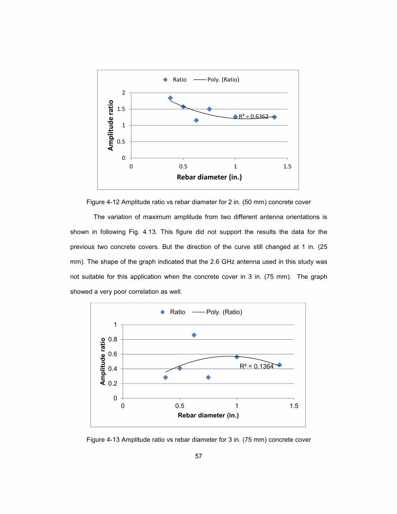
57
Figure 4-12 Amplitude ratio vs rebar diameter for 2 in. (50 mm) concrete cover The variation of maximum amplitude from two different antenna orientations is
shown in following Fig. 4.13. This figure did not support the results the data for the
previous two concrete covers. But the direction of the curve still changed at 1 in. (25
mm). The shape of the graph indicated that the 2.6 GHz antenna used in this study was
not suitable for this application when the concrete cover in 3 in. (75 mm). The graph
showed a very poor correlation as well.
Figure 4-13 Amplitude ratio vs rebar diameter for 3 in. (75 mm) concrete cover
R² = 0.6362
0
0.5
1
1.5
2
0 0.5 1 1.5
Am
pli
tud
e r
ati
o
Rebar diameter (in.)
Ratio Poly. (Ratio)
R² = 0.1364
0
0.2
0.4
0.6
0.8
1
0 0.5 1 1.5
Am
plitu
de r
ati
o
Rebar diameter (in.)
Ratio Poly. (Ratio)

58
4.6.4 Diameter Estimation from maximum positive amplitude
The maximum positive amplitude from the normal orientation of the antenna can
be used to estimate the diameter of the rebar. The maximum positive amplitude form the
90⁰ polarized position of the rebar cannot be used as a parameter to estimate rebar
because of its change of behavior with cover depth was not consistent as shown in Fig.
4.8 and 4.9. The ratio of maximum amplitude also cannot be used a parameter to
estimate the rebar diameter due to inconsistent shape of the amplitude ratio vs diameter
curve as shown in Fig. 4.10, 4.11 and 4.12. Utsi et al. (2004) used numerical model to
establish a relationship between the maximum amplitudes and the diameter of the rebar
but their numerical model were not verified by experimental data. They also did not
consider the effect of changing dielectric constant on amplitude vs diameter relationship.
A numerical model was developed to establish a relationship between the
maximum positive amplitude and the rebar diameter. Six different numerical models were
run to obtain maximum positive amplitude from six different diameters that were used in
the beam specimen. GPRMAX 2D (Giannopoulos, 2003) was used as a software
package to run the electromagnetic simulation. The model was run with a dielectric
constant of 7 which was similar to the beam specimen. The rebar were placed at a cover
depth of 2 in. (50 mm) in the numerical model. The normalized maximum positive
amplitudes were recorded form the numerical modeling data for each different diameter
of the rebar. The raw GPR data were taken into RADAN and only background removal
filter were applied on the data. After applying the background removal filter, the maximum
positive normalized amplitudes were recorded from RADAN for each of the different
diameters of the rebars at 2 in. (50 mm) concrete cover. The normalized amplitudes were
collected in a scale between 0 to 1. A normalized amplitude of 0.15 means that the
maximum positive amplitude from the rebar is 15% of the overall maximum amplitude of

59
the scan. The normalized amplitudes were also converted to normalized decibel using
the equation dB=20log10(Normalized Amplitude). Table 4.3 shows the experimental and
the numerical data of maximum positive amplitudes. It was observed that the numerical
values of maximum amplitudes very close but less than the experimental values of
maximum amplitudes. The minimum change in normalized dB was 2.96% for #5 rebar
and the minimum change in normalized dB was 12.32% for #8 rebar. Both the
experimental and numerical values of maximum normalized amplitudes were increasing
with the increase in rebar diameter. The detail information of numerical modeling of GPR
wave is discussed in chapter 5.
Table 4-3 Comparison of experimental and numerical data
Rebar Dia
Dia (in.) GPRMAX
Data GPRMAX
(dB) Experimental Data(RADAN)
Experimental Data (dB)
% dB Change
#3 0.375 0.1335 -17.4904 0.149108 -16.53 5.81
#4 0.5 0.15332 -16.2878 0.161808 -15.82 2.96
#5 0.625 0.1714 -15.3198 0.201372 -13.92 10.06
#6 0.75 0.19607 -14.1518 0.231473 -12.71 11.34
#8 1 0.23741 -12.49 0.277971 -11.12 12.32
#11 1.375 0.30972 -10.1808 0.298882 -10.49 2.95
The maximum normalized positive amplitudes from the rebars from numerical
model and the experimental data are plotted in Fig. 4.14.

60
Figure 4-14 Rebar diameter vs maximum normalized amplitude for numerical and experimental data
In Fig. 4.14, the linear regression equations for both numerical and the
experimental data for rebar diameter vs maximum normalized amplitudes are shown. The
numerical data was showing a correlation of 99.81% which indicated an almost perfect
linear correlation between the rebar diameter and the maximum positive amplitude. The
experimental data were very close to numerical data with a correlation coefficient of
93.02%. The linear regression equation for experimental data were also developed and
shown on Fig. 4.14. The numerical and the experimental regression curves, both can be
used to estimate the rebar diameter within an accuracy of 20%.
4.7 Diameter Estimation using Empirical Approach
The existing techniques of diameter estimation using GPR are discussed in
chapter 2. In this part of the study, the empirical approach using digital numeric image by
Chang et al. (2009) was used to estimate the diameter of the rebar. According to Chang
GPRMAX Numerical data
y = 0.1764x + 0.0642
R² = 0.9981
Experimental Data
y = 0.1602x + 0.0966
R² = 0.9302
0
0.05
0.1
0.15
0.2
0.25
0.3
0.35
0 0.2 0.4 0.6 0.8 1 1.2 1.4 1.6
GPRMAX Data Read GPR Data
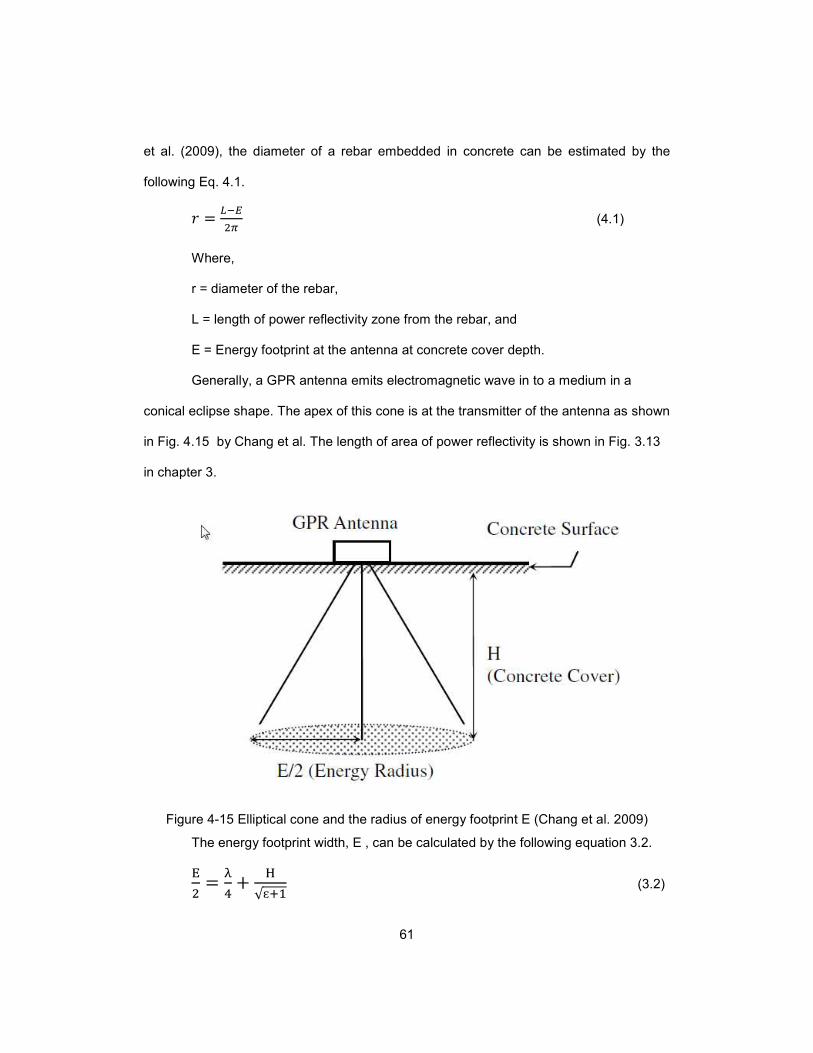
61
et al. (2009), the diameter of a rebar embedded in concrete can be estimated by the
following Eq. 4.1.
/ = ;<�= (4.1)
Where,
r = diameter of the rebar,
L = length of power reflectivity zone from the rebar, and
E = Energy footprint at the antenna at concrete cover depth.
Generally, a GPR antenna emits electromagnetic wave in to a medium in a
conical eclipse shape. The apex of this cone is at the transmitter of the antenna as shown
in Fig. 4.15 by Chang et al. The length of area of power reflectivity is shown in Fig. 3.13
in chapter 3.
Figure 4-15 Elliptical cone and the radius of energy footprint E (Chang et al. 2009)
The energy footprint width, E , can be calculated by the following equation 3.2.
> = ?@ + A√ɛB� (3.2)
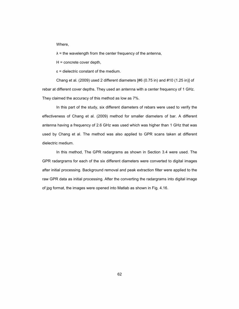
62
Where,
λ = the wavelength from the center frequency of the antenna,
H = concrete cover depth,
ɛ = dielectric constant of the medium.
Chang et al. (2009) used 2 different diameters [#6 (0.75 in) and #10 (1.25 in)] of
rebar at different cover depths. They used an antenna with a center frequency of 1 GHz.
They claimed the accuracy of this method as low as 7%.
In this part of the study, six different diameters of rebars were used to verify the
effectiveness of Chang et al. (2009) method for smaller diameters of bar. A different
antenna having a frequency of 2.6 GHz was used which was higher than 1 GHz that was
used by Chang et al. The method was also applied to GPR scans taken at different
dielectric medium.
In this method, The GPR radargrams as shown in Section 3.4 were used. The
GPR radargrams for each of the six different diameters were converted to digital images
after initial processing. Background removal and peak extraction filter were applied to the
raw GPR data as initial processing. After the converting the radargrams into digital image
of jpg format, the images were opened into Matlab as shown in Fig. 4.16.

63
Figure 4-16 GPR radargram in Matlab
The GPR images were converted in to alpha numeric code as shown in Fig. 4.17.
Figure 4-17 Digitized image in Matlab
The box area as shown in Fig. 4.17 was zoomed out to see the numeric codes as
shown in Fig. 4.18. These numeric codes were used as the basis of estimating the initial
point of power reflectivity. Where there was a significant difference in the numeric values
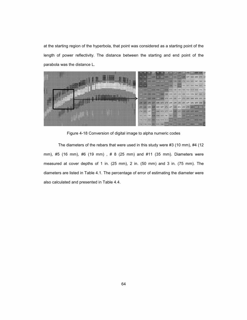
64
at the starting region of the hyperbola, that point was considered as a starting point of the
length of power reflectivity. The distance between the starting and end point of the
parabola was the distance L.
Figure 4-18 Conversion of digital image to alpha numeric codes
The diameters of the rebars that were used in this study were #3 (10 mm), #4 (12
mm), #5 (16 mm), #6 (19 mm) , # 8 (25 mm) and #11 (35 mm). Diameters were
measured at cover depths of 1 in. (25 mm), 2 in. (50 mm) and 3 in. (75 mm). The
diameters are listed in Table 4.1. The percentage of error of estimating the diameter were
also calculated and presented in Table 4.4.

65
Table 4-4 Estimation of rebar diameter by Chang et al. (2009) method
Rebar Dia
Cover (in.)
E (in) L (in) Dia (in.) Error(%)
#3
1 1.139 4.03 0.46 22.7
2 1.944 4.6 0.42 12.7
3 2.7 4.7 0.32 15.1
#4
1 1.139 4.41 0.52 4.1
2 1.944 5.28 0.53 1.5
3 2.7 6.52 0.61 5.4
#5
1 1.139 4.8 0.58 6.8
2 1.944 5.86 0.62 0.3
3 2.7 6.75 0.64 3.1
#6
1 1.139 6.72 0.89 18.4
2 1.944 7.2 0.84 11.5
3 2.7 7.39 0.75 0.5
#8
1 1.139 5.95 0.77 23.4
2 1.944 7.77 0.93 7.3
3 2.7 8.35 0.90 10.1
#11
1 1.139 7.3 0.98 28.7
2 1.944 8.06 0.97 29.2
3 2.7 9.6 1.10 20.1
Table 4.4 showed that for #3 (10 mm) rebar, the error of estimating the diameter
was 22.7%. For #4 (12 mm) and #5 (16 mm) rebar, the error was 5.4% and 6.8%
respectively. But for #6 (19 mm), #8 (25 mm) and # 11 (35 mm) rebars, the error
percentages were 18.4%, 23.4% and 29.2% respectively. From the above data, it was
concluded that the 2.6 GHz antenna was useful for estimating diameter for #4 (12 mm)
and #5 (16 mm) dia rebars. Any diameters greater or less than these two diameters were
not accurate enough. Chang et al. (2009) found a good accuracy of 7% for #6 (19 mm)
and #10 (32 mm) rebars using 1 GHz antenna. So, to estimate diameter of rebars greater
than #5 (16 mm) dia, 1 GHz antenna was the better option. For diameters of #3 (10 mm)
and smaller bars, a higher frequency greater than 2.6 GHz is recommended.
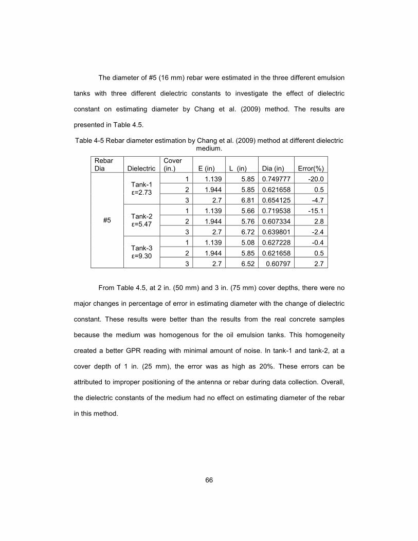
66
The diameter of #5 (16 mm) rebar were estimated in the three different emulsion
tanks with three different dielectric constants to investigate the effect of dielectric
constant on estimating diameter by Chang et al. (2009) method. The results are
presented in Table 4.5.
Table 4-5 Rebar diameter estimation by Chang et al. (2009) method at different dielectric medium.
Rebar Dia Dielectric
Cover (in.) E (in) L (in) Dia (in) Error(%)
#5
Tank-1 ε=2.73
1 1.139 5.85 0.749777 -20.0
2 1.944 5.85 0.621658 0.5
3 2.7 6.81 0.654125 -4.7
Tank-2 ε=5.47
1 1.139 5.66 0.719538 -15.1
2 1.944 5.76 0.607334 2.8
3 2.7 6.72 0.639801 -2.4
Tank-3 ε=9.30
1 1.139 5.08 0.627228 -0.4
2 1.944 5.85 0.621658 0.5
3 2.7 6.52 0.60797 2.7
From Table 4.5, at 2 in. (50 mm) and 3 in. (75 mm) cover depths, there were no
major changes in percentage of error in estimating diameter with the change of dielectric
constant. These results were better than the results from the real concrete samples
because the medium was homogenous for the oil emulsion tanks. This homogeneity
created a better GPR reading with minimal amount of noise. In tank-1 and tank-2, at a
cover depth of 1 in. (25 mm), the error was as high as 20%. These errors can be
attributed to improper positioning of the antenna or rebar during data collection. Overall,
the dielectric constants of the medium had no effect on estimating diameter of the rebar
in this method.
67
4.7 Discussion
In this chapter, first, three GPR parameters were investigated and their effect on
the size of the rebar was studied. The three parameters were:
a) Maximum positive reflection amplitude of GPR wave form normal antenna
orientation,
b) Maximum positive reflection amplitude of GPR wave form 90˚ polarized
antenna orientation,
c) Ratio of amplitude mentioned in (a) and (b) above.
The results presented in this chapter showed that the normal antenna orientation
displayed a steady relation between the maximum amplitude and the size of the rebar at
1 in. (25 mm) and 2 in. (25 mm) depth. The polarized orientation of the antenna showed
inconsistent response at 1 in. (25 mm) and 2 in. (25 mm) depth. The parameter of ratio
between maximum amplitude in two perpendicular antenna orientations was not suitable
for the ranges of diameter that was used. It was showing consistent behavior at deeper
concrete cover.
The diameter of the rebar was estimated using two different methods. First, the
rebar diameters were measured by establishing a relationship between the maximum
positive amplitude from the rebar and the rebar diameter. Both the numerical and
experimental data were very close and showed good correlations. Second, the rebar
diameters were measured using an empirical approach using digital image processing. It
was observed that this method is sensitive to the antenna frequency and the antenna
used in this study was good for the diameter of #4 (12 mm) and #5 (16mm). For rebar
diameter greater than #5 (16mm), a lower frequency antenna was recommended. For
rebar diameter less than #4 (12 mm), a higher frequency antenna was recommended.

68
In next phase of this study, the change in cross sectional area in a rebar due to
corrosion in investigated using GPR. Based on the results shown in this chapter, the
maximum positive amplitude of the reflected wave form rebar was taken as the principal
GPR parameter that was sensitive to size of the rebar.

69
Chapter 5
Effect of various GPR parameters on corroded rebar in concrete
5.1 Introduction
In this phase of the study, the variation of GPR response over the different
corrosion state of rebar embedded in concrete was investigated. Rebars were corroded
in an accelerated environment and a novel method of simulating the corrosion in
laboratory using oil tank was developed. The effect of concrete dielectric constant on
GPR response was also investigated. The dielectric constant of concrete at different
stages of its service life was also simulated in the laboratory using oil water emulsions as
a substitute of concrete. Eventually the amount of loss of mass from rebar due to
corrosion was related to maximum amplitude of GPR response from the corroded bar.
5.2 Oil Tank as a substitute of concrete beam specimen
In the previous chapter, the change of GPR response for different diameter of
rebars was discussed. But one parameter was not investigated, which was the
electromagnetic property of concrete. According to RADAR theory, speed and
characteristics of the propagation of electromagnetic wave through any medium depends
on the dielectric constant of the medium. The value of dielectric constant of a medium
can range from 1 (air) to 81 (water) and every other material falls in between. The
dielectric constants of normal cooking oils (canola, vegetable, sunflower seeds etc.) are
close to dielectric constant of concrete. Maser (2003) showed in a study that an oil tank
with a particular thickness could be used as a substitute of a concrete sample with
equivalent thickness. Moreover the dielectric constant of the oil could be manipulated by
adding water to the oil with the help of emulsifying agent.

70
5.2.1 Preparation of oil tank
Three oil tanks were made to conduct this study. The dielectric properties of oil of
these three tanks were different. This first tank was filled with oil only. The second and
third tank was filled with oil water emulsion of different proportions to simulate different
dielectric property. The emulsion of tank-3 had more water content than tank-2, which
made the tank-3 dielectric constant higher than that in tank-2. The thickness of the oil and
emulsions in the three tanks was 5 in. (125 mm). A plexiglas cover was placed over the
oil surface of each tank to facilitate the movement of radar antenna and to make the
antenna ground coupled with the oil surface. An oil tank, representative of a 5 in. (125
mm) thick concrete beam is shown in Fig. 5.1.
Figure 5-1 Oil tank as a substitute of concrete beam
An arrangement was made, as shown in Fig. 5.2, to support the plexiglas cover
over the oil surface and to accommodate the rebars into the oil tank at a different depth.
Three different depth of 1 in. (25 mm), 2 in. (50 mm), and 3 in. (75 mm) were taken as
concrete clear cover as it was for the real concrete beam specimen in the previous
chapter.

71
Figure 5-2 Arrangement to hold rebars in oil tank to simulate concrete cover
Two other tanks were prepared using oil emulsion. The emulsions were made by
adding water with the oil. Water has a very high dielectric constant of 81. So adding a
small amount of water could increase the dielectric constant of the emulsion by a
significant amount. When concrete is dry and sound, amount of free water in concrete is
almost zero, and the concrete has a very high resistivity resulting in a very low dielectric
constant. As concrete gets older, water can enter into the interstitial spaces into concrete
through cracks or damages caused by weathering and deteriorating effects. This
presence of water into concrete increases it dielectric constant. So if an oil-only tank
represents a dry concrete beam, then an oil water emulsion tank with particular
consistency will be representative of old concrete. When GPR scan is performed to
investigate an old structure, it is important to know how the behavior of GPR response
change under this variable dielectric constants of the concrete.
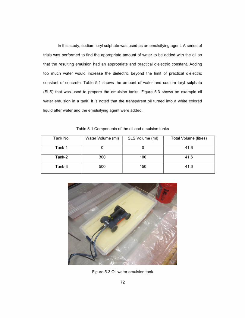
72
In this study, sodium loryl sulphate was used as an emulsifying agent. A series of
trials was performed to find the appropriate amount of water to be added with the oil so
that the resulting emulsion had an appropriate and practical dielectric constant. Adding
too much water would increase the dielectric beyond the limit of practical dielectric
constant of concrete. Table 5.1 shows the amount of water and sodium loryl sulphate
(SLS) that was used to prepare the emulsion tanks. Figure 5.3 shows an example oil
water emulsion in a tank. It is noted that the transparent oil turned into a white colored
liquid after water and the emulsifying agent were added.
Table 5-1 Components of the oil and emulsion tanks
Tank No. Water Volume (ml) SLS Volume (ml) Total Volume (litres)
Tank-1 0 0 41.6
Tank-2 300 100 41.6
Tank-3 500 150 41.6
Figure 5-3 Oil water emulsion tank
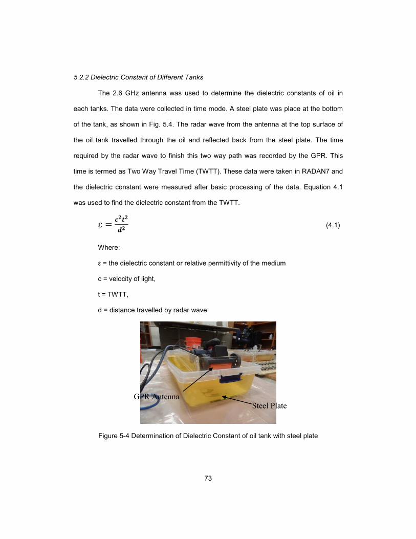
73
5.2.2 Dielectric Constant of Different Tanks
The 2.6 GHz antenna was used to determine the dielectric constants of oil in
each tanks. The data were collected in time mode. A steel plate was place at the bottom
of the tank, as shown in Fig. 5.4. The radar wave from the antenna at the top surface of
the oil tank travelled through the oil and reflected back from the steel plate. The time
required by the radar wave to finish this two way path was recorded by the GPR. This
time is termed as Two Way Travel Time (TWTT). These data were taken in RADAN7 and
the dielectric constant were measured after basic processing of the data. Equation 4.1
was used to find the dielectric constant from the TWTT.
ɛ = CDEDFD (4.1)
Where:
ε = the dielectric constant or relative permittivity of the medium
c = velocity of light,
t = TWTT,
d = distance travelled by radar wave.
Figure 5-4 Determination of Dielectric Constant of oil tank with steel plate
Steel Plate GPR Antenna

74
In Fig. 5.5, the radargram of the three tanks are shown. The horizontal axis is the
number of scans and the vertical axis isthe two way travel time.The bright reflection in
each of the radar gram was the reflection from the steel plate. It is obvious that the radar
wave was taking more time to travel the same distance as it proceeded from tank-1 to
tank-3. So it is obvious that the velocity of GPR wave was highest in tank-1 because the
TWTT for the GPR wave is lowest. Similarly the speed of radar wave was slowest in
tank-3 because the TWTT was highest. The TWTTs for the tanks were converted to
dielectric constants using the conversion equation. The values are listed in Table 5.2.
Tank-1 Tank-2 Tank-3
Figure 5-5 Radargrams of the three tanks
Bottom of the
tank
Bottom of the
tank
Bottom of the
tank

75
Table 5-2 TWTT and dielectric constant of different tanks
Tank TWTT (nS) Dielectric Constant
1 1.4 2.73
2 1.98 5.47
3 2.58 9.3
5.3 Validation of oil tank as a substitute of concrete beam
The three oil tanks were representative of concrete beams with dielectric
constants of 2.73, 5.47 and 9.3, respectively. Steel rebars of three different diameters
were placed in each tank. The diameters of the rebars were #3, #4 and #5 (10, 12 and 16
mm dia). The rebars were placed at three different depths of 1 in. (25 mm), 2 in. (50 mm),
and 3 in.(75 mm) in the liquid. GPR scans were performed for each depth of the rebar
into the tanks. It was expected that the GPR radargram of the rebar in oil tank would be
similar to GPR radargram of rebar embedded in real concrete beam, as observed in the
previous phase of this study.
There were two major advantages of using the oil tanks instead of real concrete
beam. First, it is really difficult to make concrete with variable dielectric constants. So,
using water emulsion was very helpful to see the effect of dielectric constant on GPR
response. Second, concrete is a heterogeneous material and its dielectric constant is not
exactly same everywhere. The dielectric constant of concrete is the resultant of the
dielectric constants of its components, which are coarse/fine aggregates and cement
paste. Using oil or oil-water emulsion was helpful to eliminate the uncertainty due to
spatial variability of dielectric constant of concrete. Third, there was great flexibility of
placing the rebar of different diameters and for different cover depths in a single water

76
tank. If concrete sample were made, lots of beams should have been constructed. The oil
tanks eliminated the use of additional time and resources for making real concrete
samples. So, the repetitive use of the tank for different rebar size and different cover
depth was a great advantage. Figure 5.6 shows a GPR plot that was collected from the
oil tank-1 with a #4 (12 mm dia) rebar at 2 in. (50 mm) depth from the top surface of the
oil. It is observed that the radargram is exactly similar to a radargram of a real concrete
specimen. The oscilloscope view was also obtained for the trace having maximum
amplitude. As oil was a homogenous material, the amount of noise in the data was much
less compare to data collected from real concrete sample. Therefore, it was validated that
the oil tanks could be used as a substitute of concrete beams.
Figure 5-6 GPR Radargram data collected form oil tank.
5.4 Plot of the collected data to verify the performance of the oil tanks
As mentioned earlier, three different diameters of rebars were used in each of the
three tanks at three different cover depths. The maximum amplitudes from the radargram
were recorded. Figure 5.7 shows the rebars that were used in the tank to record the GPR
Peak normalized
amplitude from
rebar

77
data. The GPR parameters of data collection are listed in Table 5.3. The collected data
are tabulated in Table 5.4.
Figure 5-7 Rebars used in the oil and emulsion tanks
Table 5-3 GPR parameters for data collection
Scan per second (horizontal direction) 325
Scan per unit inch (horizontal direction) 20.38
Sample per scan (vertical direction) 256
Time range in vertical Direction 7 nS
#5 #4 #3
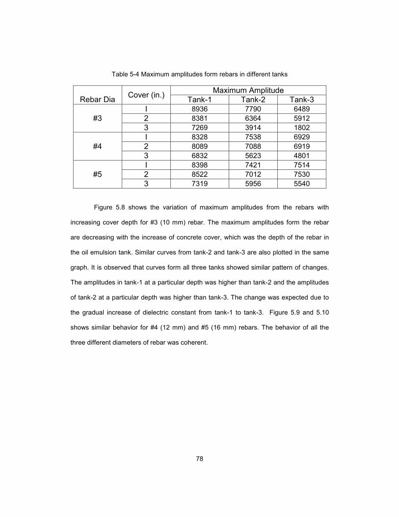
78
Table 5-4 Maximum amplitudes form rebars in different tanks
Rebar Dia
Cover (in.) Maximum Amplitude
Tank-1 Tank-2 Tank-3
#3
I 8936 7790 6489
2 8381 6364 5912
3 7269 3914 1802
#4
I 8328 7538 6929
2 8089 7088 6919
3 6832 5623 4801
#5
I 8398 7421 7514
2 8522 7012 7530
3 7319 5956 5540
Figure 5.8 shows the variation of maximum amplitudes from the rebars with
increasing cover depth for #3 (10 mm) rebar. The maximum amplitudes form the rebar
are decreasing with the increase of concrete cover, which was the depth of the rebar in
the oil emulsion tank. Similar curves from tank-2 and tank-3 are also plotted in the same
graph. It is observed that curves form all three tanks showed similar pattern of changes.
The amplitudes in tank-1 at a particular depth was higher than tank-2 and the amplitudes
of tank-2 at a particular depth was higher than tank-3. The change was expected due to
the gradual increase of dielectric constant from tank-1 to tank-3. Figure 5.9 and 5.10
shows similar behavior for #4 (12 mm) and #5 (16 mm) rebars. The behavior of all the
three different diameters of rebar was coherent.

79
Figure 5-8 Amplitude vs cover depth for #3 (10 mm) rebar
Figure 5-9 Amplitude vs cover depth for #4 (12 mm) rebar
0
1000
2000
3000
4000
5000
6000
7000
8000
9000
10000
0 0.5 1 1.5 2 2.5 3 3.5
Am
pli
tud
es
Concrete Cover (in.)
Tank-1 Tank-2 Tank-3
4000
4500
5000
5500
6000
6500
7000
7500
8000
8500
9000
0 1 2 3 4
Am
pli
tud
es
Concrete Cover (in.)
Tank-1 Tank-2 Tank-3

80
Figure 5-10 Amplitude vs cover depth for #5 (16 mm) rebar
Figure 5.11 shows the change of maximum amplitude from a #3 (10 mm) rebar
with different dielectric constants. Similar graphs are produced for #4 (12 mm) rebar and
#5 (16 mm) rebar, as shown in Fig. 5.12 and Fig. 5.13. The amplitudes decreased with
the increase of dielectric constant at different depths. All three different diameters of
rebar showed coherent behavior as displayed in in Fig. 5.11 to Fig. 5.13.
4000
5000
6000
7000
8000
9000
10000
0 1 2 3 4
Am
pli
tud
es
Concrete Cover (in.)
Tank-1 Tank-2 Tank-3

81
Figure 5-11 Amplitude vs dielectric constant for #3 (10 mm) rebar
Figure 5-12 Amplitude vs dielectric constant for #4 (12 mm) rebar
0
1000
2000
3000
4000
5000
6000
7000
8000
9000
10000
0 2 4 6 8 10
Am
pli
tud
e
Dielectric constant
1 in.
2 in.
3 in.
0
1000
2000
3000
4000
5000
6000
7000
8000
9000
0 2 4 6 8 10
Am
pli
tud
e
Dielectric constant
1 in.
2 in.
3 in.
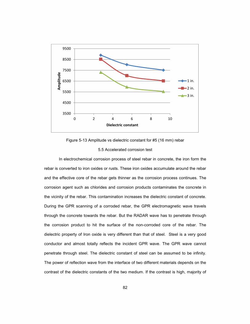
82
Figure 5-13 Amplitude vs dielectric constant for #5 (16 mm) rebar
5.5 Accelerated corrosion test
In electrochemical corrosion process of steel rebar in concrete, the iron form the
rebar is converted to iron oxides or rusts. These iron oxides accumulate around the rebar
and the effective core of the rebar gets thinner as the corrosion process continues. The
corrosion agent such as chlorides and corrosion products contaminates the concrete in
the vicinity of the rebar. This contamination increases the dielectric constant of concrete.
During the GPR scanning of a corroded rebar, the GPR electromagnetic wave travels
through the concrete towards the rebar. But the RADAR wave has to penetrate through
the corrosion product to hit the surface of the non-corroded core of the rebar. The
dielectric property of Iron oxide is very different than that of steel. Steel is a very good
conductor and almost totally reflects the incident GPR wave. The GPR wave cannot
penetrate through steel. The dielectric constant of steel can be assumed to be infinity.
The power of reflection wave from the interface of two different materials depends on the
contrast of the dielectric constants of the two medium. If the contrast is high, majority of
3500
4500
5500
6500
7500
8500
9500
0 2 4 6 8 10
Am
pli
tud
e
Dielectric constant
1 in.
2 in.
3 in.

83
the incident wave get reflected and a small part of the wave go through the interface. IF
the dielectric contrast is low, a small part of the incident wave gets reflected and the
majority of the incident wave travels through the interface into the second medium. The
dielectric constant of Iron Oxide is 14 which is very close to the dielectric constant of
concrete. This close difference of dielectric constant between the steel and concrete
indicates that radar wave does not totally reflect from the surface of Iron Oxide. Rather it
penetrates through the Iron Oxides (corrosion product) and eventually get reflected from
the surface of non-corroded core of the rebar. Therefore It can be concluded that GPR
wave can travel through the corrosion products. The changed environment in the vicinity
of a corroded rebar can be monitored using GPR. In this phase of the research, the
change in GPR responses with respect to the amount of corrosion was studied.
The schematic diagram of GPR scanning of a corroded rebar in concrete is
shown in Fig. 5.14. The dielectric constant of the space between the GPR antenna and
the non-corroded core of the rebar increases due to the contamination of the concrete by
external corrosion agents and the internal development of corrosion products. The
thinning of rebar and the increase of the dielectric constant of the concrete are the two
major factors that can differentiate the GPR response form a corroded rebar from that of
a non-corroded rebar. It was expected that the increase of dielectric constant and
decrease of size of the rebar would result in a decrease in the maximum amplitude form
the rebar.

84
Figure 5-14 Schematic diagram of GPR scanning of corroded rebar
5.6 Corrosion Tank
A corrosion tank was prepared to perform the accelerated corrosion of three #5
dia (16 mm) rebars. The tank was filled with 5% sodium chloride solution. Regular table
salt was used for sodium chloride and tap water was used to prepare the solution. The #5
(16 mm) rebars were submerged into the solution to act as anode of an electrochemical
cell. Some extra rebar were also submerged in the salt water solution to act as a
cathode. A switch board was used to give electrical connections to the cathode. The
switches of the switch board were in a parallel connection. The three #5 (16 mm) rebars
were connected in series. The series connection ensured that the first of the three rebar
will attract more electrical current which created the most amount of electrochemical
reaction in the first rebar. The other two rebars, as they were connected in series
connection, were having less electrical current resulting in less amount of corrosion. That
GPR
Antenna
non-corroded
Core of Rebar Corrosion
Product
(Iron Oxides)
T R

85
was how difference in amount of corrosion in the three different rebars was ensured. A
DC current source was used to supply electrical current to the electrochemical cell
through anodes and the cathodes. The positive end from the DC source was connected
to the anode which is the three #5 (16 mm) rebars that were connected in series. The
negative end of the DC power source was connected with the cathode rebars through the
switch boards. A 12 Volt potential difference was created between the anode and the
cathode rebars using the DC power source. The experimental setup of the accelerated
corrosion of the rebars in salt water is shown in Fig. 5.15. The corrosion products are
seen floating on the salt water solution. The cathode rebars were connected with 10 KΩ
resistors to protect the circuit. The DC power source and the resistors are shown in Fig
5.16.
Figure 5-15 Corrosion tank for accelerated corrosion

86
Figure 5-16 DC power source and 10 KΩ resistor
The corrosion process was run for a week. After one week the current flow was
stopped and the anode rebars were taken out of the corrosion tank. They were
thoroughly cleaned. Figure 5.17 shows the three #5 (16 mm) rebars with a non-corroded
rebar on the left side for comparison. It was obvious that the three #5 (16 mm) rebars
were corroded in different amount due to the difference in amount of current flow among
the rebars.
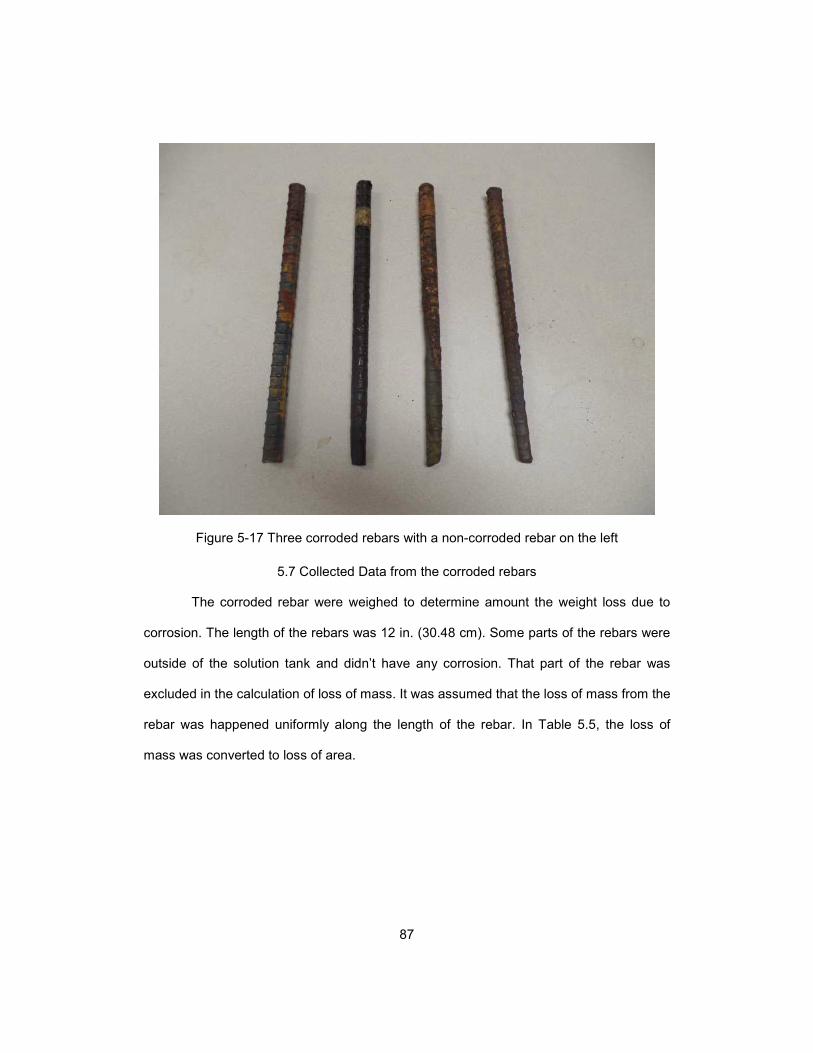
87
Figure 5-17 Three corroded rebars with a non-corroded rebar on the left
5.7 Collected Data from the corroded rebars
The corroded rebar were weighed to determine amount the weight loss due to
corrosion. The length of the rebars was 12 in. (30.48 cm). Some parts of the rebars were
outside of the solution tank and didn’t have any corrosion. That part of the rebar was
excluded in the calculation of loss of mass. It was assumed that the loss of mass from the
rebar was happened uniformly along the length of the rebar. In Table 5.5, the loss of
mass was converted to loss of area.

88
Table 5-5 Amount of mass loss in #5 (16 mm) rebars
Rebar Initial Mass
(g)
Mass after corrosion (g)
Loss (g)
Length of Corroded part of 12 in. long
rebar (in.)
Avg. Area
Loss %
Rebar-1 472 472 0 0 0
Rebar-2 472 394 78 7 22
Rebar-3 472 363 109 6 31
Reabr-4 472 310 162 6 45
After weighing the rebars, each of them were taken to the oil emulsion tanks as
shown in Fig. 4.18. The data collection parameters were similar to as listed in Table 5.3.
Each rebar was placed in the emulsion tanks. The placement of the corroded rebar in an
emulsion tank was assumed to be similar to a real corroded rebar embedded in
concrete. The GPR scanning was performed on each of the corroded rebar as shown in
Fig. 5.19. The B-Scans or radargrams for each rebar were recorded for different tanks
and different depth at each tank. For each rebar, 9 sets of data were collected. A total of
27 sets of scanning were performed on the corroded rebars. Data were also taken for the
non-corroded rebar to compare with the corroded rebars. The GPR B-Scans were taken
into RADAN to post-process the data.

89
Figure 5-18 Oil emulation tanks for corroded rebar
Figure 5-19 GPR Data collection from the corroded rebar in oil emulsion tank

90
Background removal function was applied to all the data. The maximum
amplitude and the corresponding two way travel times were recorded for each of the
scans. The collected data are presented in Table 5.6. According to Table 5.5, Rebar-1
was without any corrosion and the amount of corrosion gradually increased from Rebar-2
to Rebar-4.
Table 5-6 Processed data of the corroded rebars in corrosion tanks
Rebar-1
Rebar-2
Scan TWTT(nS) Amplitude Depth(in)
Scan TWTT(nS) Amplitude
Depth (in)
Tank-1
71 0.36 17861 1
Tank-1
2267 0.39 13363 1
460 0.64 11194 2 2681 0.64 8514 2
871 0.89 7252 3 3095 0.89 5642 3
Tank-2
1153 0.45 13343 1
Tank-2
1159 0.54 8570 1
1543 0.76 7424 2 1560 0.86 4845 2
1944 1.08 3153 3 1960 1.14 2560 3
Tank-3
2211 0.57 9326 1
Tank-3
92 0.64 7728 1
2558 0.98 4960 2 504 1.04 3990 2
2945 1.42 3506 3 925 1.42 2317 3
Rebar-3
Rebar-4
Scan TWTT(nS) Amplitude Depth(in)
Scan TWTT(nS) Amplitude Depth(in)
T
ank-1
93 0.42 13215 1
Tank-1
2263 0.43 10696 1
518 0.67 8130 2 2696 0.67 6922 2
899 0.92 5583 3 3116 0.93 4716 3
Tank-2
1131 0.54 7662 1
Tank-2
1192 0.51 7586 1
1500 0.86 4955 2 1580 0.82 4347 2
1849 1.11 2665 3 1971 1.17 1685 3
Tank-3
2119 0.7 6654 1
Tank-3
98 0.73 5972 1
2520 1.08 3848 2 508 1.11 3263 2
2930 1.48 2028 3 901 1.48 1503 3
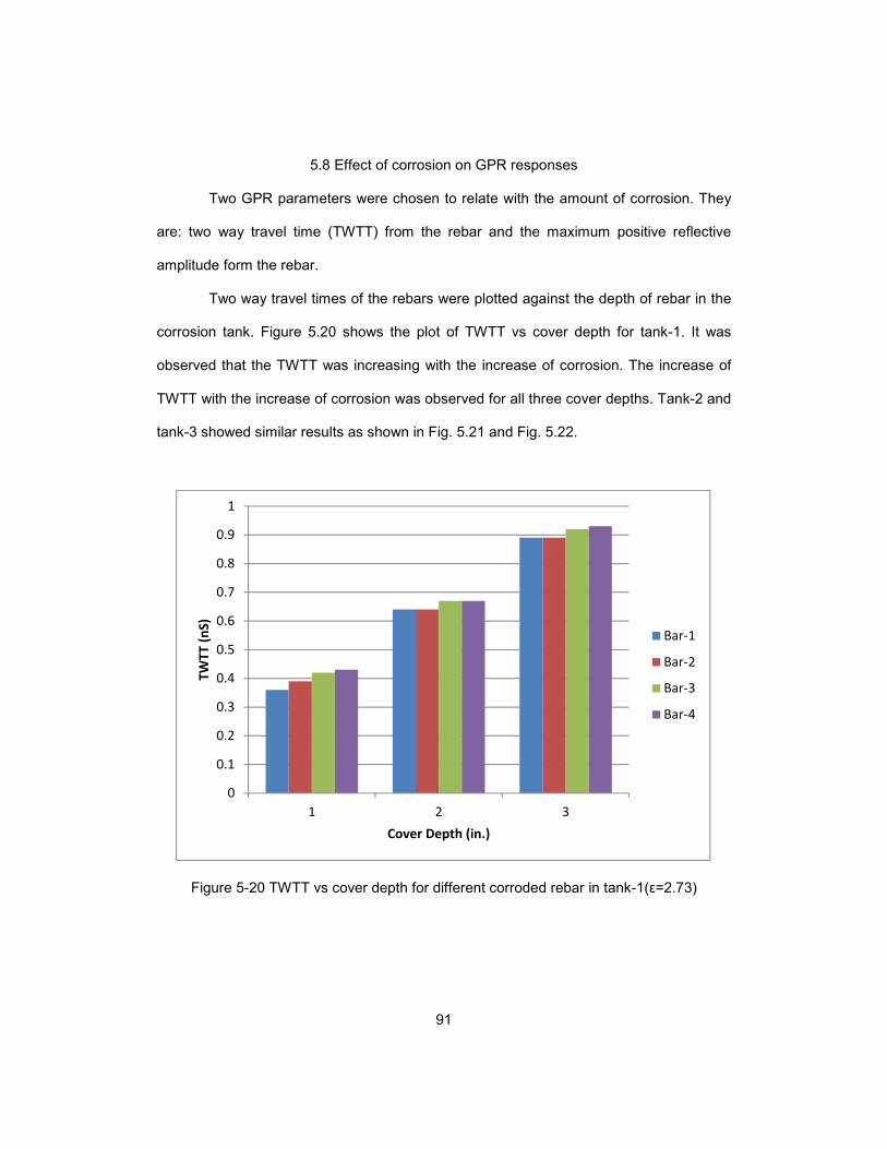
91
5.8 Effect of corrosion on GPR responses
Two GPR parameters were chosen to relate with the amount of corrosion. They
are: two way travel time (TWTT) from the rebar and the maximum positive reflective
amplitude form the rebar.
Two way travel times of the rebars were plotted against the depth of rebar in the
corrosion tank. Figure 5.20 shows the plot of TWTT vs cover depth for tank-1. It was
observed that the TWTT was increasing with the increase of corrosion. The increase of
TWTT with the increase of corrosion was observed for all three cover depths. Tank-2 and
tank-3 showed similar results as shown in Fig. 5.21 and Fig. 5.22.
Figure 5-20 TWTT vs cover depth for different corroded rebar in tank-1(ε=2.73)
0
0.1
0.2
0.3
0.4
0.5
0.6
0.7
0.8
0.9
1
1 2 3
TW
TT
(n
S)
Cover Depth (in.)
Bar-1
Bar-2
Bar-3
Bar-4

92
Figure 5-21 TWTT vs cover depth for different corroded rebar in tank-2 (ε=5.47)
Figure 5-22 TWTT vs cover depth for different corroded rebar in tank-3 (ε=9.3)
0
0.2
0.4
0.6
0.8
1
1.2
1.4
1 2 3
TW
TT
(n
S)
Cover Depth (in.)
Bar-1
Bar-2
Bar-3
Bar-4
0
0.2
0.4
0.6
0.8
1
1.2
1.4
1.6
1 2 3
TW
TT
(n
S)
Cover Depth (in.)
Bar-1
Bar-2
Bar-3
Bar-4

93
The maximum positive reflection amplitudes of the rebars were plotted against
the depth of rebar for each of the corrosion tank. Figure 5.23 shows the plot of maximum
amplitude vs cover depth for tank-1. It is observed that the maximum amplitude was
decreasing with the increase of corrosion. The decrease of maximum amplitude with the
increase of corrosion was observed for all three cover depths. Tank-2 and tank-3 showed
similar results as shown in Fig. 5.24 and Fig. 5.25.
Figure 5-23 Maximum amplitude vs cover depth for different corroded rebar in tank-1 (ε=2.73)
0
2000
4000
6000
8000
10000
12000
14000
16000
18000
20000
1 2 3
Am
pli
tud
e
Cover Depth (in.)
Bar-1
Bar-2
Bar-3
Bar-4
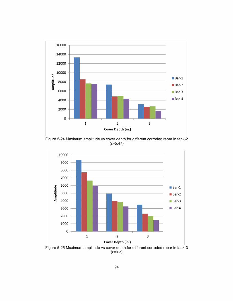
94
Figure 5-24 Maximum amplitude vs cover depth for different corroded rebar in tank-2
(ε=5.47)
Figure 5-25 Maximum amplitude vs cover depth for different corroded rebar in tank-3
(ε=9.3)
0
2000
4000
6000
8000
10000
12000
14000
16000
1 2 3
Am
pli
tud
e
Cover Depth (in.)
Bar-1
Bar-2
Bar-3
Bar-4
0
1000
2000
3000
4000
5000
6000
7000
8000
9000
10000
1 2 3
Am
pli
tud
e
Cover Depth (in.)
Bar-1
Bar-2
Bar-3
Bar-4
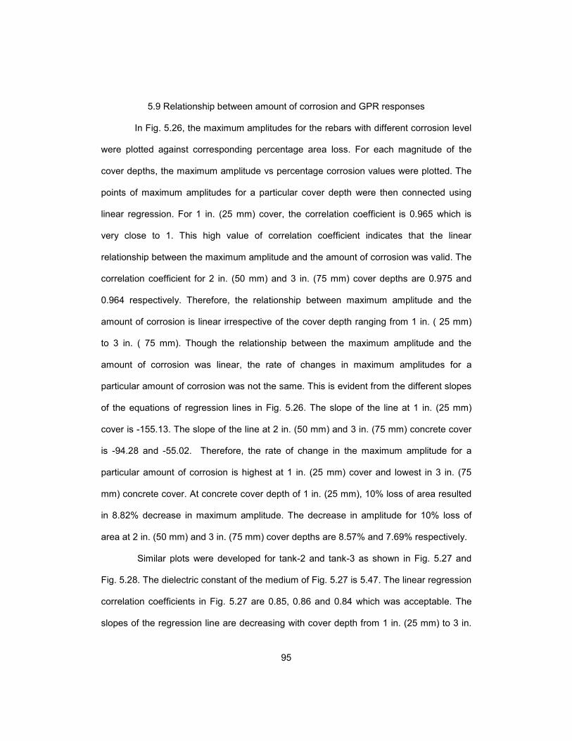
95
5.9 Relationship between amount of corrosion and GPR responses
In Fig. 5.26, the maximum amplitudes for the rebars with different corrosion level
were plotted against corresponding percentage area loss. For each magnitude of the
cover depths, the maximum amplitude vs percentage corrosion values were plotted. The
points of maximum amplitudes for a particular cover depth were then connected using
linear regression. For 1 in. (25 mm) cover, the correlation coefficient is 0.965 which is
very close to 1. This high value of correlation coefficient indicates that the linear
relationship between the maximum amplitude and the amount of corrosion was valid. The
correlation coefficient for 2 in. (50 mm) and 3 in. (75 mm) cover depths are 0.975 and
0.964 respectively. Therefore, the relationship between maximum amplitude and the
amount of corrosion is linear irrespective of the cover depth ranging from 1 in. ( 25 mm)
to 3 in. ( 75 mm). Though the relationship between the maximum amplitude and the
amount of corrosion was linear, the rate of changes in maximum amplitudes for a
particular amount of corrosion was not the same. This is evident from the different slopes
of the equations of regression lines in Fig. 5.26. The slope of the line at 1 in. (25 mm)
cover is -155.13. The slope of the line at 2 in. (50 mm) and 3 in. (75 mm) concrete cover
is -94.28 and -55.02. Therefore, the rate of change in the maximum amplitude for a
particular amount of corrosion is highest at 1 in. (25 mm) cover and lowest in 3 in. (75
mm) concrete cover. At concrete cover depth of 1 in. (25 mm), 10% loss of area resulted
in 8.82% decrease in maximum amplitude. The decrease in amplitude for 10% loss of
area at 2 in. (50 mm) and 3 in. (75 mm) cover depths are 8.57% and 7.69% respectively.
Similar plots were developed for tank-2 and tank-3 as shown in Fig. 5.27 and
Fig. 5.28. The dielectric constant of the medium of Fig. 5.27 is 5.47. The linear regression
correlation coefficients in Fig. 5.27 are 0.85, 0.86 and 0.84 which was acceptable. The
slopes of the regression line are decreasing with cover depth from 1 in. (25 mm) to 3 in.

96
(75 mm). For 10% loss of area at 1 in. (25 mm), the maximum amplitude decreased by
10.64%. The change in amplitude for 10% loss of area at 2 in. (50 mm) and 3 in. (75 mm)
are 9.63% and 9.16%. The dielectric constant of the medium is 9.3 at Fig. 5.28 In Fig.
5.28, correlation coefficient of the linear regression lines at 1 in. (25 mm), 2 in. (50 mm)
and 3 in. (75 mm) concrete cover are 0.984, 0.986 and 0.986 respectively. This high
value of correlation coefficient confirms that the relation between the maximum
amplitudes and the loss of area is linear. The slope of the regression line at 1 in. (25 mm)
depth is highest. The change of maximum amplitudes for 10% loss of area at 1 in. (25
mm), 2 in. (50 mm) and 3 in. (75 mm) cover depths are 8.26%, 7.52% and 12.99%
respectively.
Figure 5-26 Maximum amplitude vs percentage area loss in tank-1 (ε = 2.73)
y = -155.13x + 17584
R² = 0.965
y = -94.286x + 11000
R² = 0.9757
y = -55.015x + 7146.1
R² = 0.9643
0
2000
4000
6000
8000
10000
12000
14000
16000
18000
20000
0 10 20 30 40 50
Am
pli
tud
e
Percentage Area Loss (%)
1 in.
2 in.
3 in.

97
Figure 5-27 Maximum amplitude vs percentage area loss in tank-2 (ε = 5.47)
Figure 5-28 Maximum amplitude vs percentage area loss in tank-3 (ε = 9.3)
y = -133.78x + 12568
R² = 0.8504
y = -67.988x + 7058.5
R² = 0.8652
y = -29.732x + 3244.2
R² = 0.8434
0
2000
4000
6000
8000
10000
12000
14000
16000
0 10 20 30 40 50
Am
pli
tud
e
Percentage Area Loss (%)
1 in.
2 in.
3 in.
y = -76.829x + 9302.3
R² = 0.9842
y = -37.036x + 4922.6
R² = 0.9861
y = -44.617x + 3431.6
R² = 0.9861
0
1000
2000
3000
4000
5000
6000
7000
8000
9000
10000
0 10 20 30 40 50
Am
pli
tud
e
Percentage Area Loss (%)
1 in.
2 in.
3 in.

98
5.10 Proposed method to estimate the amount of corrosion
Figure 5.26 to 5.28 are very important relationship between GPR maximum
amplitude and the amount of corrosion of the rebar. This relationship can be used to
predict the existing amount of corrosion in a damaged structure with the help of GPR
scan. The following steps are recommended to estimate the amount of corrosion:
Step-1: Finding the in-situ dielectric constant of the concrete my investigative
drilling along with GPR scanning. The TWTT and the depth from drilling with provide the
in situ dielectric constant of the concrete.
Step-2: Finding the diameter of the rebar from as built drawing or ferro-scanner.
The regression equations of corrosion are given for particular diameter of rebar. This is
why knowing the diameter of the rebar is necessary to select the appropriate equation.
Step-2: Performing GPR scan on the concrete and determine the cover depth of
concrete and the maximum amplitude form the processed data.
Step-4: Estimating the amount of corrosion for pre-established linear regression
equation. Table 5.7 shows The linear regression equations for #5 (16 mm) rebar. Linear
interpolation can be applied between two cover depths and two dielectric constants in
Table 5.7.
The inputs for estimating the amount of corrosion are:
1. Concrete Cover Depth of the rebar
2. Dielectric Constant of the rebar
3. The variable ‘y’ in the regression equation which denotes the maximum
amplitude form the rebar.
The output of estimating the amount of corrosion is the variable ‘x’ which means
the percentage of mass loss from the rebar.
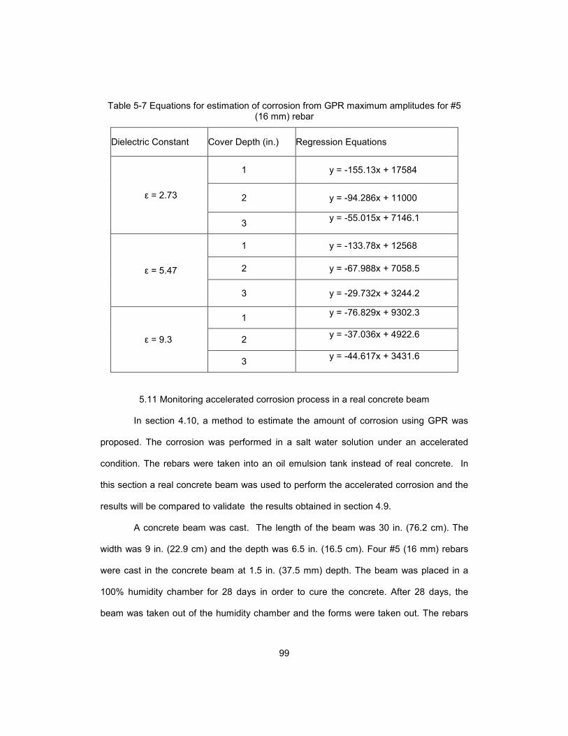
99
Table 5-7 Equations for estimation of corrosion from GPR maximum amplitudes for #5 (16 mm) rebar
Dielectric Constant Cover Depth (in.) Regression Equations
ε = 2.73
1 y = -155.13x + 17584
2 y = -94.286x + 11000
3 y = -55.015x + 7146.1
ε = 5.47
1 y = -133.78x + 12568
2 y = -67.988x + 7058.5
3 y = -29.732x + 3244.2
ε = 9.3
1 y = -76.829x + 9302.3
2 y = -37.036x + 4922.6
3 y = -44.617x + 3431.6
5.11 Monitoring accelerated corrosion process in a real concrete beam
In section 4.10, a method to estimate the amount of corrosion using GPR was
proposed. The corrosion was performed in a salt water solution under an accelerated
condition. The rebars were taken into an oil emulsion tank instead of real concrete. In
this section a real concrete beam was used to perform the accelerated corrosion and the
results will be compared to validate the results obtained in section 4.9.
A concrete beam was cast. The length of the beam was 30 in. (76.2 cm). The
width was 9 in. (22.9 cm) and the depth was 6.5 in. (16.5 cm). Four #5 (16 mm) rebars
were cast in the concrete beam at 1.5 in. (37.5 mm) depth. The beam was placed in a
100% humidity chamber for 28 days in order to cure the concrete. After 28 days, the
beam was taken out of the humidity chamber and the forms were taken out. The rebars

100
were placed in the beam in such a way that some part of the rebar would extend out of
the concrete. This was done intentionally to facilitate electrical connection to the rebar.
The beam was placed in a 5% sodium chloride solution as shown in Fig. 5.29.
Figure 5-29 Concrete beam with four #5 (16 mm) rebar in 5% salt water solution
The beam was fully submerged into sodium chloride solution for 3 days. After 3
days, the level of water was lowered just below the rebar. An accelerated corrosion
scheme was developed. Out of the 4 rebars in the beam, the middle two rebars were
used as anode and the rebars at the corners were used as cathode. As the middle two
rebar were anode, corrosion occurred in these two rebars. A 15 V DC current was
passed though the anode and the cathode. The positive end of the power source was
connected with the middle two rebars that were acting as anode. The negative end of the
power source was connected to the cathode through the switch board as discussed in
section 4.8. The experimental set-up for the accelerated corrosion is shown in Fig. 5.30.
After the corrosion started, GPR scanning of the concrete beam was performed
every 24 hours for 25 days continuously. Figure 5.31 shows the GPR scanning of the
beam using the GSSI 2600 MHz antenna. A typical B-Scan that was recorded on daily

101
basis is shown in Fig. 5.31. The four rebars were seen as hyperbolic signature in the
radargram.
Figure 5-30 Experimental set-up of accelerated corrosion
Figure 5-31 Daily data collection to monitor corrosion

102
Figure 5-32 Typical GPR Scan of the sample beam
5.12 Results of accelerated corrosion in a real concrete beam
The corrosion products were accumulating around the rebars. The concrete was
also getting damaged and its color was changed with time possibly due to chloride ion
ingression. The corroded state of the rebars at the end of 30 days is shown in Fig. 5.33.
Figure 5-33 The corroded state of the two rebars in the middle after 30 days
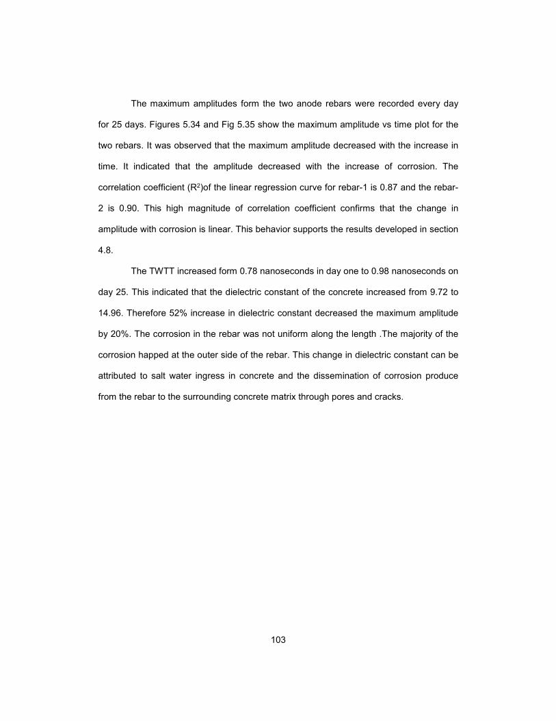
103
The maximum amplitudes form the two anode rebars were recorded every day
for 25 days. Figures 5.34 and Fig 5.35 show the maximum amplitude vs time plot for the
two rebars. It was observed that the maximum amplitude decreased with the increase in
time. It indicated that the amplitude decreased with the increase of corrosion. The
correlation coefficient (R2)of the linear regression curve for rebar-1 is 0.87 and the rebar-
2 is 0.90. This high magnitude of correlation coefficient confirms that the change in
amplitude with corrosion is linear. This behavior supports the results developed in section
4.8.
The TWTT increased form 0.78 nanoseconds in day one to 0.98 nanoseconds on
day 25. This indicated that the dielectric constant of the concrete increased from 9.72 to
14.96. Therefore 52% increase in dielectric constant decreased the maximum amplitude
by 20%. The corrosion in the rebar was not uniform along the length .The majority of the
corrosion happed at the outer side of the rebar. This change in dielectric constant can be
attributed to salt water ingress in concrete and the dissemination of corrosion produce
from the rebar to the surrounding concrete matrix through pores and cracks.
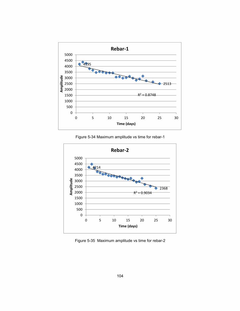
104
Figure 5-34 Maximum amplitude vs time for rebar-1
Figure 5-35 Maximum amplitude vs time for rebar-2
2513
4195
R² = 0.8748
0
500
1000
1500
2000
2500
3000
3500
4000
4500
5000
0 5 10 15 20 25 30
Am
pli
tud
e
Time (days)
Rebar-1
2368
4214
R² = 0.9034
0
500
1000
1500
2000
2500
3000
3500
4000
4500
5000
0 5 10 15 20 25 30
Am
pli
tud
e
Time (days)
Rebar-2

105
5.13 Discussion
In this chapter, a novel method to simulate long term corrosion in laboratory was
discussed. Oil emulsion tank was used as a substitute of concrete specimen. The
performance of oil emulsion tanks as s substitute of concrete beam specimen was
verified from the GPR scans. The performane of the oil tank under different diameter of
the rebar and at different concrete depth was simiar to real concrete beam. The dielectric
property of the tank was varied by controlling the amount of water in the emulsion. Three
oil water emulsion tanks were prepared with dielectric constants of 2.73, 5.47 and 9.3.
These tanks were used to observe the effect of dielectric constant on GPR response.
Accelerated corrosion of the rebar was performed in a 5% NaCl solution using
electrochemical method. The rebars were corroded at different corrosion level ranging
form 0% to 45%. The corroded rebars were placed in the oil emulsion tanks and GPR
scan was performed.
It was observed that the maximum amplitudes from the rebar decreased with the
increase of the amount of corrosion. Linear regression models were developed to
correlate between the maximum amplitudes and the percentage loss of area or corrosion.
The linear regression models were developed for three different dielectric constants
(2.73, 5.47 and 9.3) and thre different concrete cover depths [1 in. (25 mm), 2 in. (50 mm)
and 3 in. (75 mm)].
For dielectric constant of 2.73 and at concrete cover depth of 1 in. (25 mm), 10%
loss of area resulted in 8.82% decrease in maximum amplitude. The decrease in
amplitude for 10% loss of area at 2 in. (50 mm) and 3 in. (75 mm) cover depths are
8.57% and 7.69% respectively. For dielectric constant of 5.47 and for 10% loss of area at
1 in. (25 mm), the maximum amplitude decreased by 10.64%. The change in amplitude
106
for 10% loss of area at 2 in. (50 mm) and 3 in. (75 mm) are 9.63% and 9.16%. For
dielectric constant of 9.3, the change of maximum amplitudes for 10% loss of area at 1 in.
(25 mm), 2 in. (50 mm) and 3 in. (75 mm) cover depths are 8.26%, 7.52% and 12.99%
respectively.
Based on the regression model developed in this study, a method was
proposed to determine the amount of corrosion in the field. By using the cover depth,
dielectric constant and the maximum GPR amplitude as input, the quantitative amount of
corrosion can be calculated using the regression equations.
The behavior of the simulated corrosion experiment was studied by performing
another accelerated corrosion experiment using a real concrete beam. GPR maximum
amplitudes were collected for 25 days. It was observed that the maximum amplitude
decreased with time. Fifty two percent increase in dielectric constant decreased the
maximum amplitude by 20%.
107
Chapter 6
Numerical modeling
6.1 Introduction
GPR numerical modeling is very useful to develop understanding of the buried
object before actual scan is performed. The main purpose in GPR numerical modeling is
to solve the Maxwell’s electromagnetic equations. The Finite Difference Time Doman
(FTDT) method is one of the popular methods in solving the Maxwell’s equation
(Giannopoulos, 1997, 2005; Taflov, A (1995); Kunz, K.S. (1993) & Yee, K.S. (1966). The
software package used in this study is called GPRMAX (Giannopoulos, 2005). This
software package uses the FTDT method to simulate the GPR Scan. This software is
open source and available free of cost for research purposes. The experimental data
presented in chapter 3 are from complex and heterogeneous material of concrete. The
GPR responses can be affected due to this heterogeneity of concrete. In order to
understand the GPR responses in a simplistic manner, numerical modeling was
performed for the rebar in concrete where the properties of concrete were homogenous
and isotropic.
6.2 Basic concepts of GPR modeling
Any electromagnetic wave such as the RADAR wave can be expressed by the
Maxwell equations. These equations are differential equations that describe the
relationship between electrical and magnetic field quantities and their variation with
respect to the distance from the source of the electromagnetic wave. The equations are
presented in Eq. 6.1 to Eq. 6.4:

108
∇ × . = − IJI� (6.1)
∇ × K = − ILI� + M� + M� (6.2)
∇. K = 0 (6.3)
∇. L = PQ (6.4)
where,
E = electric field,
B = magnetic field,
J = current density,
t = time ,
qv = electric charge density,
D = displacement field, and
H = magnetizing field.
In order to simulate the GPR responses of a rebar embedded in concrete, the
above numerical equations need to be solved. The geometry of the medium and the
boundary conditions are also required for solution. The nature of the problem of the
above differential equations is initial value- open boundary problem (Giannopoulos,
2005). In order to perform the solution, an excitation function of the GPR antenna has to
be defined. The excitation function will define the initial condition. The resulting
electromagnetic field has to be continued until it reaches a value of zero. So there is no
specific boundary that limits the geometry of the problem. There is no known value of
electromagnetic field at any distance from the source. So this is a challenge perform the
solution within a finite space.

109
GPRMAX uses the finite difference time domain (FDTD) approach to solve the
Maxwell equations. This method discretizes the space and time. The space is discretized
spatially into elements having finite dimensions of Δx, Δy and Δz and the time is
discretized into finite Δt time units. The smaller are the spatial and temporal units; the
closer is the FDTD solution to the real solution. The FTDT approach reduces the
problem into a finite space and finite time window. The discretized elements are modeled
according to Kane Yee who introduces this method. The element that is used to mesh the
geometry of the model is called Yee cell (Yee, 1966) as show in Fig. 6.1.
Figure 6-1 Yee cell used in FTDT method (Giannopoulos, 2005)
Appropriate constitutive properties are assigned in each of the joints of Yee cell.
Complex types of shapes can be included in the model. Any curved shape will be a
staircase model as the elements are rectangular. The numerical solution is obtained by
using a discretized version of Maxwell equation. As the electromagnetic field advances
through each of the FDTD grid, a corresponding time if Δt is assumed to be elapsed.
Thus the FDTD solution simulates the electric and magnetic field for a given time window.
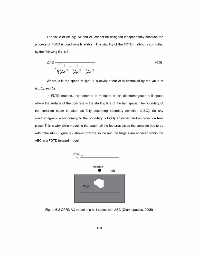
110
The value of Δx, Δy, Δz and Δt cannot be assigned independently because the
process of FDTD is conditionally stable. The stability of the FDTD method is controlled
by the following Eq. 6.5;
( ) ( ) ( )2 2 2
1
1 1 1t
cx y z
∆ ≤+ +
∆ ∆ ∆
(6.5)
Where, c is the speed of light. It is obvious that Δt is controlled by the value of
Δx, Δy and Δz.
In FDTD method, the concrete is modeled as an electromagnetic half space
where the surface of the concrete is the starting line of the half space. The boundary of
the concrete beam is taken as fully absorbing boundary condition (ABC). So any
electromagnetic wave coming to the boundary is totally absorbed and no reflection take
place. This is why while modeling the beam, all the features inside the concrete has to be
within the ABC. Figure 6.2 shows how the souce and the targets are encased within the
ABC in a FDTD forward model.
Figure 6-2 GPRMAX model of a half space with ABC (Giannopoulos, 2005)

111
6.3 Assumption of GPR modeling using GPRMAX
THe following assumptions are made while doing numerical simulation of GPR
using GPRMAX. These assumptions are mainly based on saving computational space.
• The media is linear and isotropic
• The antenna that transmits the radar wave is a line source
• The constitutive properties of the medium (dielectric property, electrical
conductivity etc.) do not vary with the frequency of the antenna.
Concrete is not an isotropic material. So modeling of concrete using GPRMAX
has limitation on this regard. The antenna is assumed as a line source which is not true
for a real antenna. Real antenna transmits a cone shaped beam of electromagnetic wave
where the apex of the cone is at the point of transmitting antenna. For constructing the
model in 2D, line source is a good assumption.
Choosing the size of mesh in FDTD method can be done by using a rule of
thumb (Giannopoulos, 2005). The rule states that the discretization step will be one tenth
of the wavelength of the antenna as shown in the following Eq. 6.6;
10l
λ∆ = (6.6)
So if the frequency of the antenna is 2600 GHz, then the minimum size of the
element used in the FDTD model will be at least 12 mm. A free space of at last 15 to 20
cells above the source is needed to ensure the absorbing boundary condition.
6.4 Input file commands
In order to build a model, a input file command is required. This file can be in
notepad or similar text file format. The input file consists of the commands that is needed
to build the geometry of the problem, defining the source antenna, assigning appropriate
constitutive properties to the geometry and commands that is needed to run the model
112
and to get desired types of output. The file then can be run in any windows operating
system using the ‘run’ command. The output is normally as ASCI file format. The main
commands to write an input file are discussed in the following sections.
6.4.1 Units
All the units that are used to express a physical dimension in GPRMAX are in
meters. The unit of time used in the input file will be in seconds. The frequency of the
source antenna will be Hertz. The origin of the coordinate system that defines the
geometry of the problem is (0, 0) and it is the lower left corner of the model.
6.4.2 Media and object construction
The medium of the model, i.e. concrete is defined by the following command.
# medium: f1 f2 f3 f4 f5 f6 str1
• f1 = Dielectric constant or relative permittivity of the medium
• f2 = relative permittivity at infinite frequency
• f3 = relaxation time of the medium
• f4 = DC conductivity of the medium
• f5 = relative permittivity of the medium
• f6 = magnetic conductivity of the medium
• str1 is used to name the medium or as a identifier of the defined medium.
If water is a medium, then by using the electric and magnetic property of water,
the GPRMAX media command can be written as:
#medium: 82.3 5.5 10.9e-12 0.0 1.0 0.0 water
To define a rectangular concrete beam, the #box command is used. The syntax
of #box command is written as:
#box: f1 f2 f3 f4 str1
where f1 and f2 is the lower left coordinates of the medium in meters. Similarly the upper
113
left of the medium is defined by the coordinate f3 and f4. The command str1 is used here
to assign property of the box that is already assigned using a medium command.
Any rebar or cylindrical object can be modeled using the # cylinder command.
The cylinder command is written as:
#cylinder: f1 f2 f3 str1
where f1 and f2 are the x and y coordinate of the center of the cylinder and f3 is the
radius of the cylinder. The command str1 is the medium identifier. If the object is a
perfectly conducting metal target like a rebar in concrete then the str1 command is written
as ‘pec’.
6.4.3 Antenna modeling
The modeling of the antenna can be done by the #line-source command as
shown below:
#line_ource: f1 f2 str1 str2
where f1 and f2 are the amplitude in amperes of the line source’s current and the
frequency in Hertz of the antenna. The parameter str1 indicates the type of excitation
function. The command str2 is used to give a user defined name to the excitation
function. The excitation function can be of many types which includes sine, Gaussian,
ricker or user defined function. The help file of the GPRMAX has the detail of the
excitation functions. An example of the excitation function command or antanna
command is:
#line_source 1.0 600e6 ricker Mysource
which specifies that the name of the antenna is Mysource. It has a frequency of
600 MHz and it produces a ricker wavelet with a amplitude of 1. In this study the ricker
excitation function is used.
The #tx command is used to define the transmitter of the antenna. It is written as:
114
#tx: f1 f2 str1 f3 f4
where f1 and f2 are the x and y coordinates in meters of the transmitter source of
the antenna. The str1 command is used to define the type of the source as discussed
earlier as ricker wavelet. The command f3 ad f4 indicate delay and removal of the source.
The #rx command indicates the receiver of the antenna and it is written as:
#rx: f1 f2
where f1 and f2 indicates the coordinate of the receiver of the antenna.
6.4.4 Domain and time window
The command #domain is used to indicate the size of the model in meters. The
command in written as:
# domain: f1 f2
where f1 and f2 are the x and y dimension of the domain in meters. The command
#dx_dy is used to define the size of the mesh of the discretized model. The #dx_dy
command is written as:
#dx_dy: f1 f2
where f1 and f2 are dimension of the mesh in x and y direction.
The command #time_window indicates the duration of the simulation. The syntax
used to define the time window is:
#time_window: f1
where f1 is the time of the simulation in seconds. Because of the very high speed of
electromagnetic wave, this quantity is normally very small and often falls within the range
of nanoseconds.
The command #analysis is used to run the analysis and save the output file. The
termination of the simulation is done using the #end_analysis command. The output
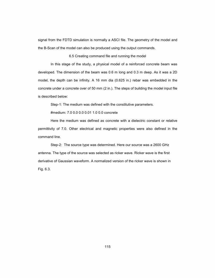
115
signal from the FDTD simulation is normally a ASCI file. The geometry of the model and
the B-Scan of the model can also be produced using the output commands.
6.5 Creating command file and running the model
In this stage of the study, a physical model of a reinforced concrete beam was
developed. The dimension of the beam was 0.6 m long and 0.3 m deep. As it was a 2D
model, the depth can be infinity. A 16 mm dia (0.625 in.) rebar was embedded in the
concrete under a concrete over of 50 mm (2 in.). The steps of building the model input file
is described below:
Step-1: The medium was defined with the constitutive parameters.
#medium: 7.0 0.0 0.0 0.01 1.0 0.0 concrete
Here the medium was defined as concrete with a dielectric constant or relative
permittivity of 7.0. Other electrical and magnetic properties were also defined in the
command line.
Step-2: The source type was determined. Here our source was a 2600 GHz
antenna. The type of the source was selected as ricker wave. Ricker wave is the first
derivative of Gaussian waveform. A normalized version of the ricker wave is shown in
Fig. 6.3.

116
Figure 6-3 Normalized ricker excitation function (Giannopoulos, 2005)
The ricker wavelet is stored in the GPRMAX as a built in function. Choosing the
frequency of the antenna is also crucial to indicate the size of the discretized elements as
discussed in section 5.2. The minimum size of the element has to be at least one tenth of
the minimum wavelength of the excitation function. The frequency that is attributed to a
GPR antenna is normally the center frequency of the band of frequencies emanating from
the antenna. The maximum frequency from an antenna is normally three times the center
frequency. So the maximum frequency of a 2600 MHz antenna will be 3X2600 = 7800
MHz. The corresponding wavelength will be 14.5 mm. So each of the element has to be
at least 1.45 mm. But in order to smoothen the curved surface of the cylinder, 1 mm was
used as the dimension of the discretized element in both x and y direction.
Step-3: The dimensions of the discretized element was
Δx =Δy = 0.001m
Step-4: The discretized time was determined.

117
0.0012.36
3 8 2t ps
e∆ = =
The value of Δt was 2.36 picoseconds. Therefore a 6 nanoseconds time window
produced 2542 iterations.
Step-5: The domain and the time window command were written.
#domain: 0.6 0.3
#dx_dy: 0.001 0.001
#time_window: 6.0e-9
The concrete box and the cylindrical rebar commands were also written. #box: 0.0 0.0 0.6 0.25 concrete
#cylinder: 0.3 0.192 0.00695 pec
Step-6: The antenna was defined using the appropriate command. The distance
between transmitter and receiver were also provided according to GSSI antenna
specification. The command to run the input file and to end the analysis was also
included.
After finishing up all the input commands, the input file was written on a notepad
file. The complete input file for the modeling of a concrete beam with a 16 mm (0.625 in.)
rebar embedded in it was composed as:
#medium: 7.0 0.0 0.0 0.01 1.0 0.0 concrete
---------------------------------------------------------------------------
#domain: 0.6 0.3
#dx_dy: 0.001 0.001
#time_window: 6.0e-9

118
---------------------------------------------------------------------------
#box: 0.0 0.0 0.6 0.25 concrete
#cylinder: 0.3 0.192 0.00695 pec
---------------------------------------------------------------------------
#line_source: 1.0 2600e6 ricker MyLineSource
#analysis: 1 rebar.txt a
#tx: 0.155 0.2525 MyLineSource 0.0 6.0e-9
#rx: 0.195 0.2525
#end_analysis:
#title: Model of rebar in concrete
#messages: y
#geometry_file: rebar.geo
6.6 Output of Simulation
The input file as shown in the previous chapter was run using GPRMAX2D. The
output signal was as ASCI file in text format. The geometry of the simulation was stored
using .geo file. The simulation was run multiple times horizontally simulating a typical
GPR scan. The resulting B-Scan was also saved in the output as .sca file. The output
ASCII file is included in Appendix A. MATLAB code were used to plot the geometry of
the model form .geo file and the B-Scan of the simulation from the .sca file. The MATLAB
code that was used in this study was generated by Bostanudin (2013). The MATLAB
codes are given in Appendix B as generated by Bostanudin (2013). The MATLAB file in
Appendix B was used in conjunction with the MATLAB file provided with GPRMAX2D
software package to generate the geometry and the B-Scan.
Figure 6.4 shows the geometry of the model. The rendition of the model
confirmed that the dimensions were correct and the rebar were placed at correct location
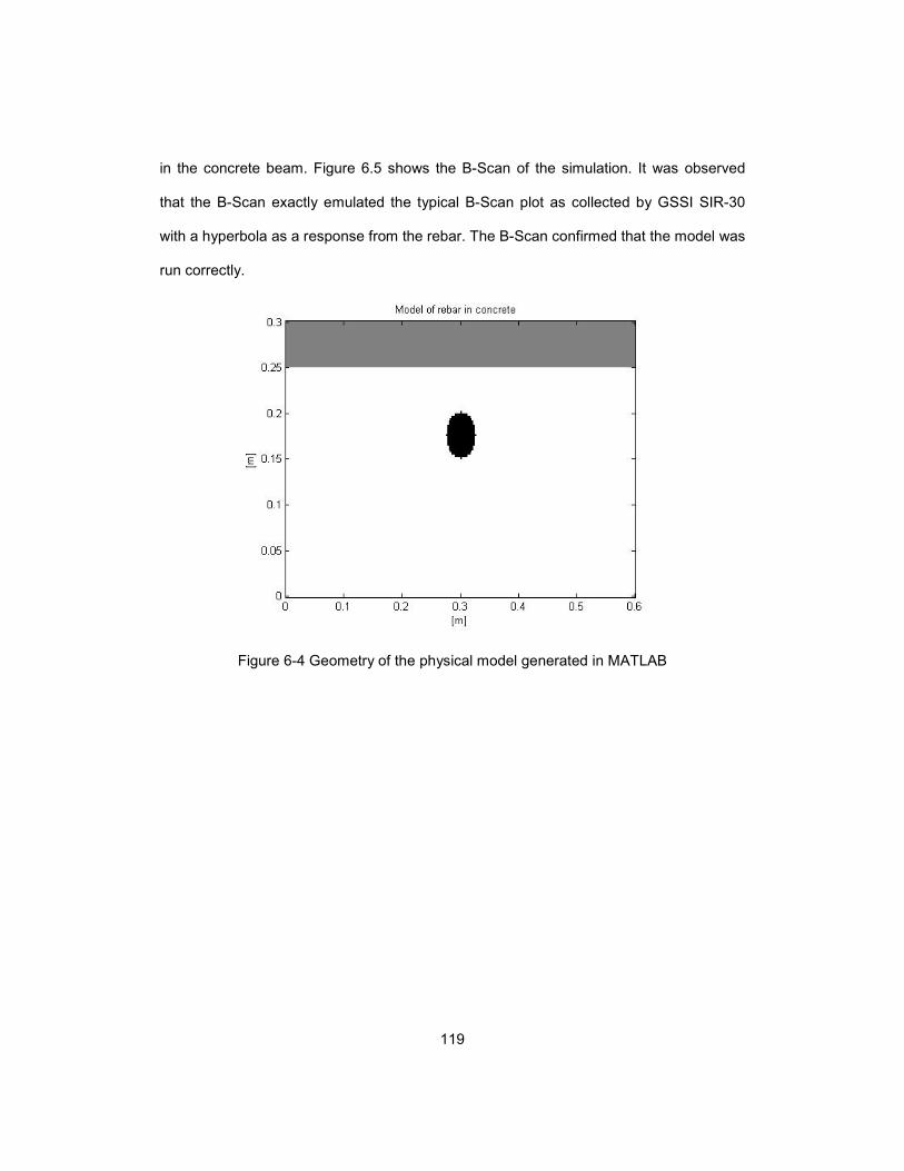
119
in the concrete beam. Figure 6.5 shows the B-Scan of the simulation. It was observed
that the B-Scan exactly emulated the typical B-Scan plot as collected by GSSI SIR-30
with a hyperbola as a response from the rebar. The B-Scan confirmed that the model was
run correctly.
Figure 6-4 Geometry of the physical model generated in MATLAB
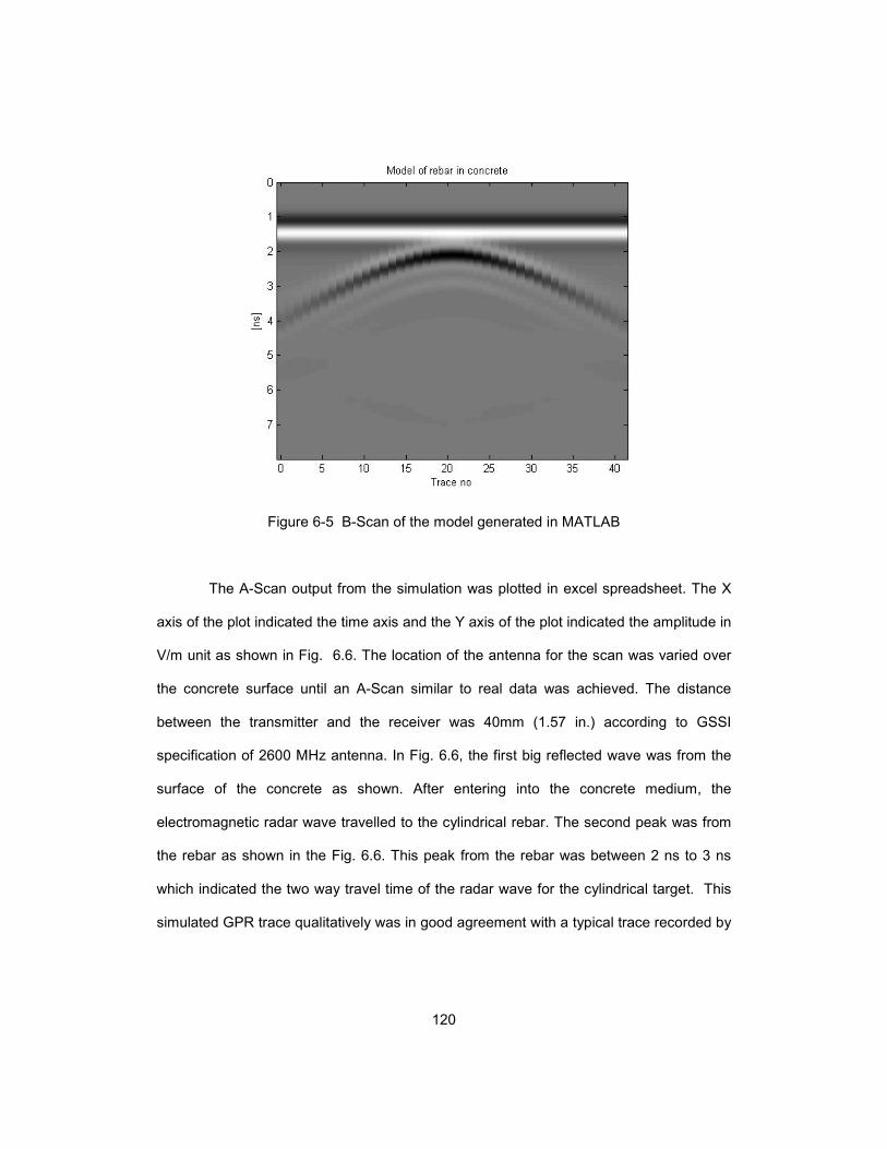
120
Figure 6-5 B-Scan of the model generated in MATLAB
The A-Scan output from the simulation was plotted in excel spreadsheet. The X
axis of the plot indicated the time axis and the Y axis of the plot indicated the amplitude in
V/m unit as shown in Fig. 6.6. The location of the antenna for the scan was varied over
the concrete surface until an A-Scan similar to real data was achieved. The distance
between the transmitter and the receiver was 40mm (1.57 in.) according to GSSI
specification of 2600 MHz antenna. In Fig. 6.6, the first big reflected wave was from the
surface of the concrete as shown. After entering into the concrete medium, the
electromagnetic radar wave travelled to the cylindrical rebar. The second peak was from
the rebar as shown in the Fig. 6.6. This peak from the rebar was between 2 ns to 3 ns
which indicated the two way travel time of the radar wave for the cylindrical target. This
simulated GPR trace qualitatively was in good agreement with a typical trace recorded by
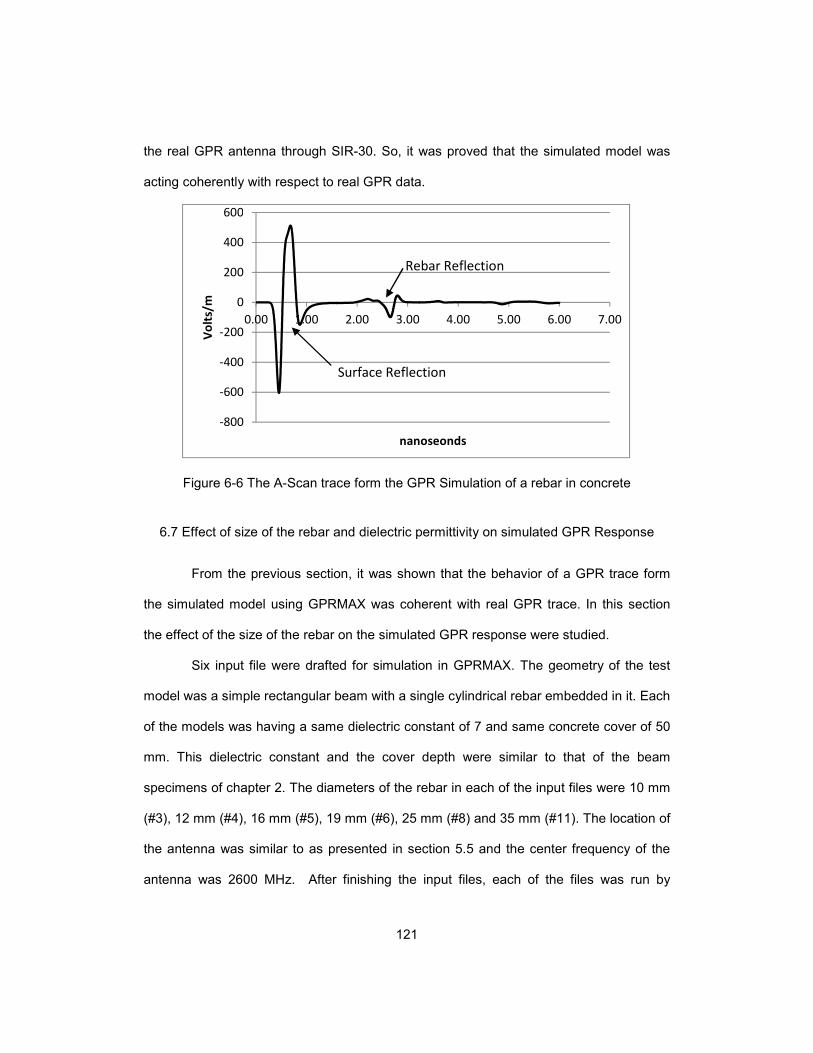
121
the real GPR antenna through SIR-30. So, it was proved that the simulated model was
acting coherently with respect to real GPR data.
Figure 6-6 The A-Scan trace form the GPR Simulation of a rebar in concrete
6.7 Effect of size of the rebar and dielectric permittivity on simulated GPR Response
From the previous section, it was shown that the behavior of a GPR trace form
the simulated model using GPRMAX was coherent with real GPR trace. In this section
the effect of the size of the rebar on the simulated GPR response were studied.
Six input file were drafted for simulation in GPRMAX. The geometry of the test
model was a simple rectangular beam with a single cylindrical rebar embedded in it. Each
of the models was having a same dielectric constant of 7 and same concrete cover of 50
mm. This dielectric constant and the cover depth were similar to that of the beam
specimens of chapter 2. The diameters of the rebar in each of the input files were 10 mm
(#3), 12 mm (#4), 16 mm (#5), 19 mm (#6), 25 mm (#8) and 35 mm (#11). The location of
the antenna was similar to as presented in section 5.5 and the center frequency of the
antenna was 2600 MHz. After finishing the input files, each of the files was run by
-800
-600
-400
-200
0
200
400
600
0.00 1.00 2.00 3.00 4.00 5.00 6.00 7.00
Vo
lts/
m
nanoseonds
Rebar Reflection
Surface Reflection

122
GPRMAX and the output traces were recorded. The output ASCI files were then
converted to excel files and each of the A-Scan traces was normalized and plotted in a
single graph. The two way travel time was on X axis and the normalized amplitude was
on the Y axis in the plot. The resulting plot is shown in Fig. 6.7. It was observed that the
amplitude of the surface reflections or direct waves were same for all six traces. But the
differences in reflections from the rebars were prominent. The part from Fig. 6.7 that
shows the reflection from the rebar is highlighted by a circle. The circled part of Fig. 6.7 is
blown up and shown in Fig. 6.8. From Fig. 6.8 it was obvious that the higher was the
diameter of the rebar, the higher was the normalized reflection amplitude. The 35 mm
(#11) rebar was showing larger reflection amplitude than the 25 mm (#8) rebar. Similarly
the 25 mm (#8) rebar was showing larger reflection amplitude than the 19 mm (#6) rebar
and so forth. These responses form the simulated model were in good agreement with
real GPR traces as discussed in chapter 3 and chapter 4.
Figure 6-7 Simulated GPR traces from six different rebars by GPRMAX
-1.50
-1.00
-0.50
0.00
0.50
1.00
0.0 1.0 2.0 3.0 4.0 5.0 6.0 7.0
No
rma
lize
d A
mp
litu
de
Time (nS)
#3 Rebar #4 Rebar #5 Rebar
#6 Rebar #8 Rebar #11 Rebar
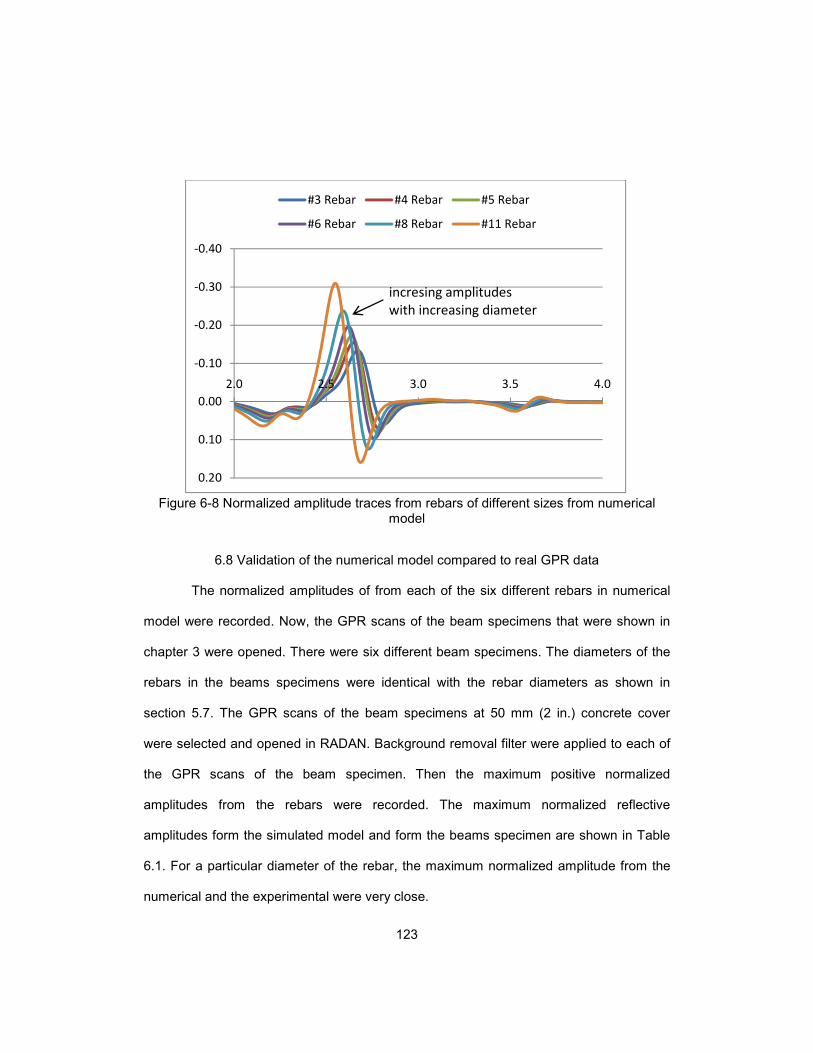
123
Figure 6-8 Normalized amplitude traces from rebars of different sizes from numerical
model
6.8 Validation of the numerical model compared to real GPR data
The normalized amplitudes of from each of the six different rebars in numerical
model were recorded. Now, the GPR scans of the beam specimens that were shown in
chapter 3 were opened. There were six different beam specimens. The diameters of the
rebars in the beams specimens were identical with the rebar diameters as shown in
section 5.7. The GPR scans of the beam specimens at 50 mm (2 in.) concrete cover
were selected and opened in RADAN. Background removal filter were applied to each of
the GPR scans of the beam specimen. Then the maximum positive normalized
amplitudes from the rebars were recorded. The maximum normalized reflective
amplitudes form the simulated model and form the beams specimen are shown in Table
6.1. For a particular diameter of the rebar, the maximum normalized amplitude from the
numerical and the experimental were very close.
-0.40
-0.30
-0.20
-0.10
0.00
0.10
0.20
2.0 2.5 3.0 3.5 4.0
#3 Rebar #4 Rebar #5 Rebar
#6 Rebar #8 Rebar #11 Rebar
incresing amplitudes
with increasing diameter
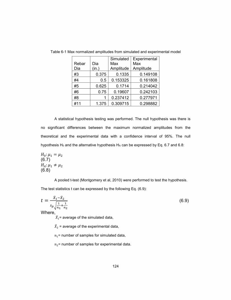
124
Table 6-1 Max normalized amplitudes from simulated and experimental model
Rebar Dia
Dia (in.)
Simulated Max Amplitude
Experimental Max Amplitude
#3 0.375 0.1335 0.149108
#4 0.5 0.153325 0.161808
#5 0.625 0.1714 0.214042
#6 0.75 0.19607 0.242103
#8 1 0.237412 0.277971
#11 1.375 0.309715 0.298882
A statistical hypothesis testing was performed. The null hypothesis was there is
no significant differences between the maximum normalized amplitudes from the
theoretical and the experimental data with a confidence interval of 95%. The null
hypothesis H0 and the alternative hypothesis HA can be expressed by Eq. 6.7 and 6.8:
K%: �� = � (6.7) KS: �� ≠ � (6.8)
A pooled t-test (Montgomery et al, 2010) were performed to test the hypothesis.
The test statistics t can be expressed by the following Eq. (6.9):
� = UVW<UV��XY WZWB WZ� (6.9)
Where, [V�= average of the simulated data,
[V = average of the experimental data,
\�= number of samples for simulated data,
\= number of samples for experimental data.
125
The pooled variance ]̂ is expressed by the following Eq. 6.11:
]̂ = (_W<�)�W�B(_�<�)���_WB_�< (6.11)
Where, ]�= variance of the simulated data,
]= variance of the experimental data.
The test statistics t was calculated as -0.54 from Eq. 6.9. The rejection criteria
was determined from the t-table (Montgomery et al, 2010) for the degree of freedom and
expected level of significance. The rejection criteria for the null hypothesis was 2.228t >
and 2.228t < − .
The test statistics t, was not falling in the rejection region. So we failed to reject
the null hypothesis.
Therefore we accept the null hypothesis.
Based on the pooled t-test, it was concluded that there was no significant
difference between the numerical and the experimental data with a confidence interval of
95%.
6.8 Effect of dielectric permittivity on simulated GPR Response
To test the effect of dielectric constant on simulated GPR model, three input files
were prepared. The geometry of the file consisted of rectangular concrete space with 16
mm (#5) rebar embedded in it. The antenna was having a frequency of 2600 MHz. The
only differences among the three input files were the dielectric constant. The three input
files were having a dielectric constant of 7, 10 and 13 respectively. After running the input
files in GPRMAX, the output traces were plotted. All three traces were plotted in a single
126
plot to understand the effect of dielectric constant. The resulting plot is shown in Fig. 6.9.
It was obvious that the higher is the dielectric constant, the higher was the two way travel
time and the reflection amplitude of the rebar had shifted to the right with the increase of
dielectric constant. The magnitude of the maximum amplitude from the rebar for a
dielectric constant of 7 was 69 V/m. The maximum amplitude for dielectric constant of 7
and 10 was 43 V/m and 30 V/m respectively. Though physically all three rebar were
placed at a same location, their traces are appeared at different time space in the plot.
This behavior of the simulated trace was perfectly consistent with real GPR traces.
Because the higher the dielectric constant, the slower is the speed of electromagnetic
wave. The slower velocity of the wave resulted in higher two way travel time. The
reflected amplitude of the rebars were also decreasing with increasing dielectric constant.
The surface reflection amplitude was also different for different dielectric constant. The
smaller was the dielectric constant, the higher was the surface reflection amplitude.

127
Figure 6-9 Simulated GPR traces of 16 mm (#5) rebar at different dielectric medium
In fig. 6.10, the amplitudes in Fig. 6.9 were normalized. The normalized surface
reflection or direct wave amplitudes were different in Fig. 6.10 but there were no changes
in the normalized maximum amplitudes form the rebars.
From the results that is displayed in Fig. 6.10, it was concluded that there was no
effect of the dielectric constant of the medium in the value of normalized maximum
amplitudes when the concrete cover depth and the bar diameters were constant.
-800
-600
-400
-200
0
200
400
600
0 1 2 3 4 5
Am
pli
tud
e (
V/m
)
nanoseconds
ɛ = 7 ɛ = 10 ɛ = 13
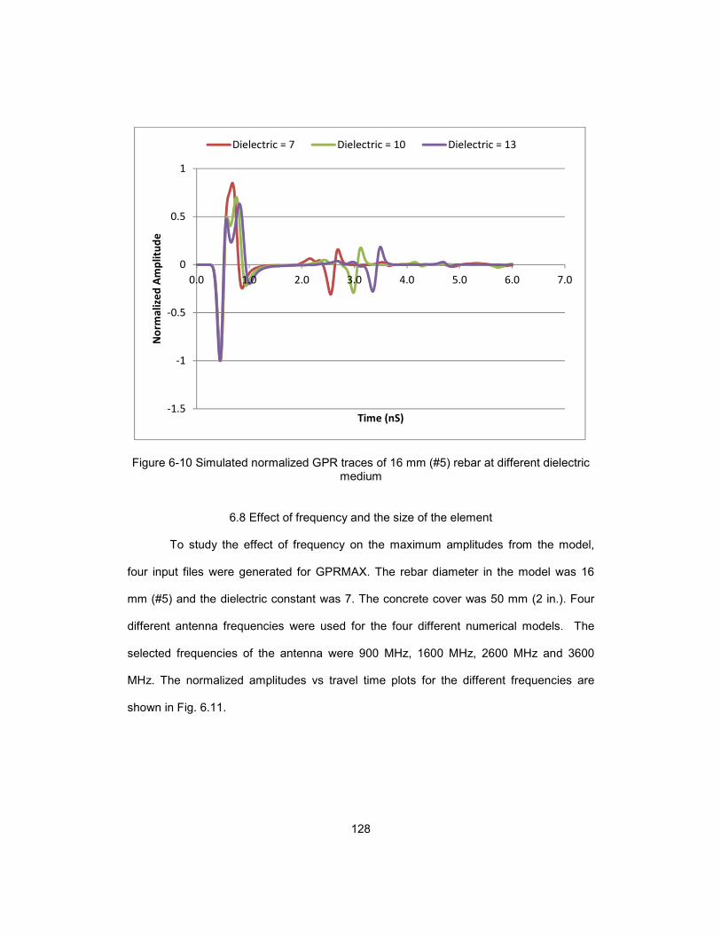
128
Figure 6-10 Simulated normalized GPR traces of 16 mm (#5) rebar at different dielectric medium
6.8 Effect of frequency and the size of the element
To study the effect of frequency on the maximum amplitudes from the model,
four input files were generated for GPRMAX. The rebar diameter in the model was 16
mm (#5) and the dielectric constant was 7. The concrete cover was 50 mm (2 in.). Four
different antenna frequencies were used for the four different numerical models. The
selected frequencies of the antenna were 900 MHz, 1600 MHz, 2600 MHz and 3600
MHz. The normalized amplitudes vs travel time plots for the different frequencies are
shown in Fig. 6.11.
-1.5
-1
-0.5
0
0.5
1
0.0 1.0 2.0 3.0 4.0 5.0 6.0 7.0
No
rma
lize
d A
mp
litu
de
Time (nS)
Dielectric = 7 Dielectric = 10 Dielectric = 13
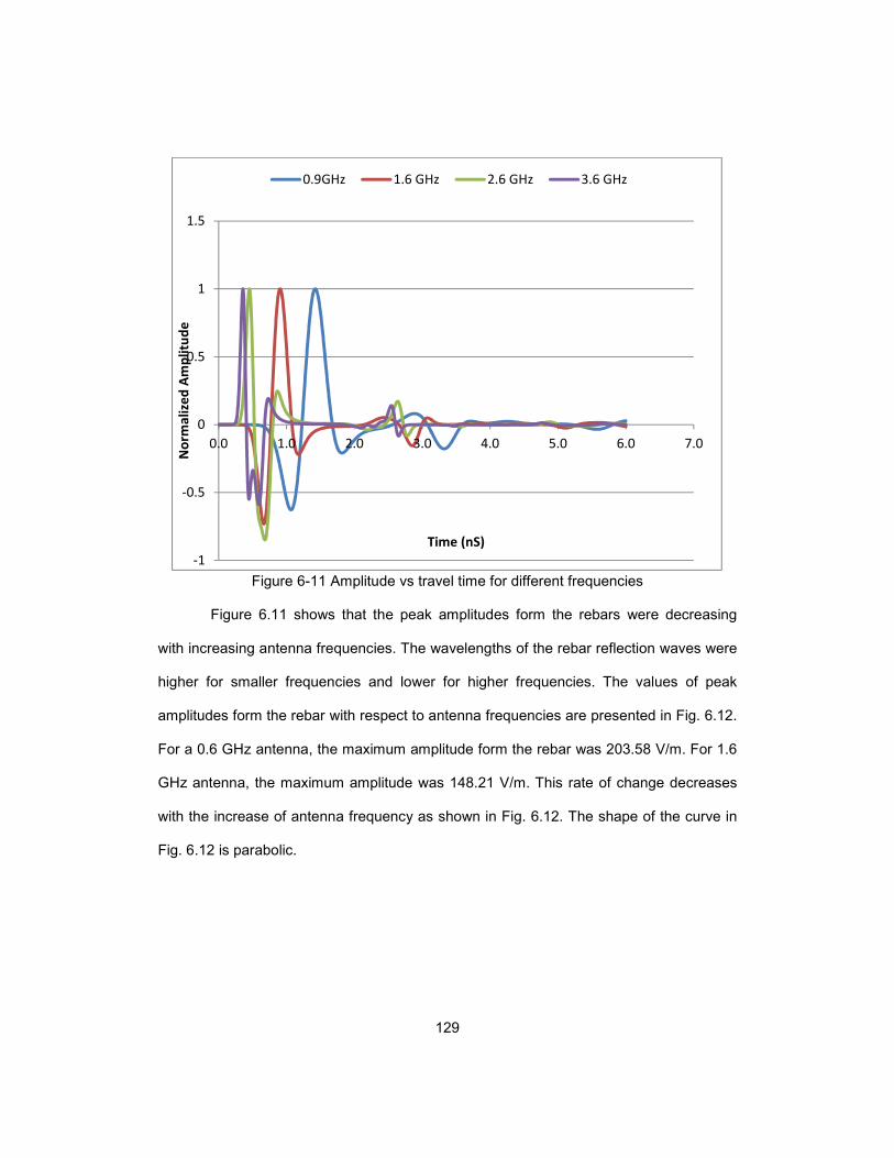
129
Figure 6-11 Amplitude vs travel time for different frequencies
Figure 6.11 shows that the peak amplitudes form the rebars were decreasing
with increasing antenna frequencies. The wavelengths of the rebar reflection waves were
higher for smaller frequencies and lower for higher frequencies. The values of peak
amplitudes form the rebar with respect to antenna frequencies are presented in Fig. 6.12.
For a 0.6 GHz antenna, the maximum amplitude form the rebar was 203.58 V/m. For 1.6
GHz antenna, the maximum amplitude was 148.21 V/m. This rate of change decreases
with the increase of antenna frequency as shown in Fig. 6.12. The shape of the curve in
Fig. 6.12 is parabolic.
-1
-0.5
0
0.5
1
1.5
0.0 1.0 2.0 3.0 4.0 5.0 6.0 7.0
No
rma
lize
d A
mp
litu
de
Time (nS)
0.9GHz 1.6 GHz 2.6 GHz 3.6 GHz
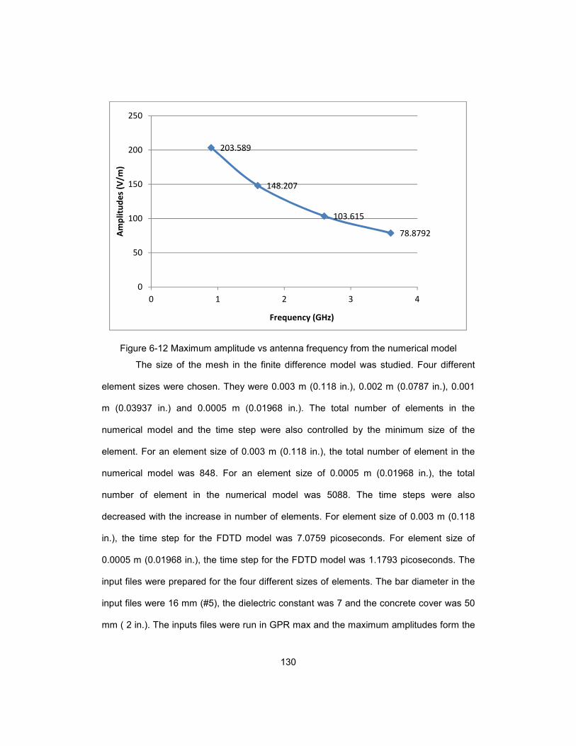
130
Figure 6-12 Maximum amplitude vs antenna frequency from the numerical model
The size of the mesh in the finite difference model was studied. Four different
element sizes were chosen. They were 0.003 m (0.118 in.), 0.002 m (0.0787 in.), 0.001
m (0.03937 in.) and 0.0005 m (0.01968 in.). The total number of elements in the
numerical model and the time step were also controlled by the minimum size of the
element. For an element size of 0.003 m (0.118 in.), the total number of element in the
numerical model was 848. For an element size of 0.0005 m (0.01968 in.), the total
number of element in the numerical model was 5088. The time steps were also
decreased with the increase in number of elements. For element size of 0.003 m (0.118
in.), the time step for the FDTD model was 7.0759 picoseconds. For element size of
0.0005 m (0.01968 in.), the time step for the FDTD model was 1.1793 picoseconds. The
input files were prepared for the four different sizes of elements. The bar diameter in the
input files were 16 mm (#5), the dielectric constant was 7 and the concrete cover was 50
mm ( 2 in.). The inputs files were run in GPR max and the maximum amplitudes form the
203.589
148.207
103.615
78.8792
0
50
100
150
200
250
0 1 2 3 4
Am
pli
tud
es
(V/m
)
Frequency (GHz)
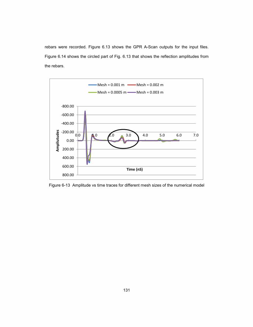
131
rebars were recorded. Figure 6.13 shows the GPR A-Scan outputs for the input files.
Figure 6.14 shows the circled part of Fig. 6.13 that shows the reflection amplitudes from
the rebars.
Figure 6-13 Amplitude vs time traces for different mesh sizes of the numerical model
-800.00
-600.00
-400.00
-200.00
0.00
200.00
400.00
600.00
800.00
0.0 1.0 2.0 3.0 4.0 5.0 6.0 7.0
Am
pli
utu
de
s
Time (nS)
Mesh = 0.001 m Mesh = 0.002 m
Mesh = 0.0005 m Mesh = 0.003 m

132
Figure 6-14 Reflection amplitudes from rebar for different sizes of elements in the numerical model
The maximum reflection amplitudes from the rebar for different element sizes are
listed in Table 6.2. The maximum amplitudes were plotted against the size of the
elements and shown in Fig. 6.15. It was observed that the maximum amplitudes from the
rebars were increasing linearly with the decreasing size of the rebar. But after the
element size was 0.001 m ( 0.03937 in.), the maximum amplitude was not increasing with
decreasing size of the element. Therefore, it was concluded that the model converged
once the size of the element is 0.001 m ( 0.03937 in.) or smaller.
Table 6-2 Maximum Amplitudes form rebars for different element sizes
Element Size (m)
Total Elements
Time Steps (picoseconds)
Max Amp V/m
0.003 848 7.0759 65.14
0.002 1272 4.7173 90.3
0.001 2544 2.3586 118.53
0.0005 5088 1.1793 118.81
-150.00
-100.00
-50.00
0.00
50.00
100.00
2.0 2.2 2.4 2.6 2.8 3.0 3.2 3.4
Mesh = 0.001 m Mesh = 0.002 m
Mesh = 0.0005 m Mesh = 0.003 m
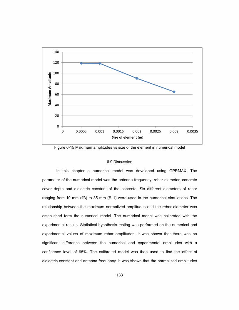
133
Figure 6-15 Maximum amplitudes vs size of the element in numerical model
6.9 Discussion
In this chapter a numerical model was developed using GPRMAX. The
parameter of the numerical model was the antenna frequency, rebar diameter, concrete
cover depth and dielectric constant of the concrete. Six different diameters of rebar
ranging from 10 mm (#3) to 35 mm (#11) were used in the numerical simulations. The
relationship between the maximum normalized amplitudes and the rebar diameter was
established form the numerical model. The numerical model was calibrated with the
experimental results. Statistical hypothesis testing was performed on the numerical and
experimental values of maximum rebar amplitudes. It was shown that there was no
significant difference between the numerical and experimental amplitudes with a
confidence level of 95%. The calibrated model was then used to find the effect of
dielectric constant and antenna frequency. It was shown that the normalized amplitudes
0
20
40
60
80
100
120
140
0 0.0005 0.001 0.0015 0.002 0.0025 0.003 0.0035
Ma
xim
um
Am
pli
tud
e
Size of element (m)

134
from the rebar did not change with the change of dielectric constants from 7 to 13 at a
particular cover depth of 50 mm (2in.). The maximum amplitudes from the rebar were
decreasing when the frequency of the antenna was increased from 0.9GHz to 3.6 GHz.
An element size analysis was also done to ensure the convergence of the numerical
model. It was found that the model converged when the element size of 0.001 m
(0.03937 in.) was used in the numerical model.

135
Chapter 7
Conclusions and Recommendations
7.1 Introduction
In this chapter, the summary of the findings of the research is presented and the
recommendation of the future study is made. In this study GPR was used as non-
destructive testing equipment to estimate the diameter of the rebar and to estimate the
quantitative loss of rebar area at different stages of corrosion. The diameters of the rebar
in concrete from GPR scan was estimated using two different approaches. The effects of
parameters such as rebar size, dielectric constant of concrete and concrete cover depth
were investigated in estimating the rebar diameter. Accelerated electrochemical corrosion
of steel rebars was performed in the laboratory at different level of corrosion. The loss of
mass from the rebars at different corrosion levels was estimated. The relation between
the GPR responses and quantitative amount of corrosion was established. The effect of
concrete dielectric constant and cover depth on the estimation of corrosion was also
studied. A FDTD numerical model of rebar in concrete was developed. The numerical
model was used to verify the experimental GPR data.
7.2 Conclusions
In this study, two methods were used to estimate the rebar diameter using GPR.
First, three GPR parameters were investigated and their effect on the size of the rebar
was studied. The three parameters were:
a) Maximum positive reflection amplitude of GPR wave form normal antenna
orientation,
b) Maximum positive reflection amplitude of GPR wave form 90˚ polarized
antenna orientation,

136
c) Ratio of amplitude mentioned in (a) and (b) above.
The results presented in this chapter showed that the normal antenna orientation
displayed a steady relation between the maximum amplitude and the size of the rebar at
1 in. (25 mm) and 2 in. (25 mm) depth. The polarized orientation of the antenna showed
inconsistent response at 1 in. (25 mm) and 2 in. (25 mm) depth. The parameter of ratio
between maximum amplitude in two perpendicular antenna orientations was not suitable
for the ranges of diameter that was used. It was showing consistent behavior at deeper
concrete cover.
The diameter of the rebar was estimated using two different methods. First, the
rebar diameters were measured by establishing a relationship between the maximum
positive amplitude from the rebar and the rebar diameter. Both the numerical and
experimental data were very close and showed good correlations. Second, the rebar
diameters were measured using an empirical approach using digital image processing. It
was observed that this method is sensitive to the antenna frequency and the antenna
used in this study was good for the diameter of #4 (12 mm) and #5 (16mm). For rebar
diameter greater than #5 (16mm), a lower frequency antenna was recommended. For
rebar diameter less than #4 (12 mm), a higher frequency antenna was recommended.
In next phase of this study, the change in cross sectional area in a rebar due to
corrosion in investigated using GPR. Based on the results shown in this chapter, the
maximum positive amplitude of the reflected wave form rebar was taken as the principal
GPR parameter that was sensitive to size of the rebar.
A novel method to simulate long term corrosion in laboratory was discussed. Oil
emulsion tank was used as a substitute of concrete specimen. The performance of oil
emulsion tanks as s substitute of concrete beam specimen was verified from the GPR
scans. The performane of the oil tank under different diameter of the rebar and at

137
different concrete depth was simiar to real concrete beam. The dielectric property of the
tank was varied by controlling the amount of water in the emulsion. Three oil water
emulsion tanks were prepared with dielectric constants of 2.73, 5.47 and 9.3. These
tanks were used to observe the effect of dielectric constant on GPR response.
Accelerated corrosion of the rebar was performed in a 5% NaCl solution using
electrochemical method. The rebars were corroded at different corrosion level ranging
form 0% to 45%. The corroded rebars were placed in the oil emulsion tanks and GPR
scan was performed.
It was observed that the maximum amplitudes from the rebar decreased with the
increase of the amount of corrosion. Linear regression models were developed to
correlate between the maximum amplitudes and the percentage loss of area or corrosion.
The linear regression models were developed for three different dielectric constants
(2.73, 5.47 and 9.3) and thre different concrete cover depths [1 in. (25 mm), 2 in. (50 mm)
and 3 in. (75 mm)].
For dielectric constant of 2.73 and at concrete cover depth of 1 in. (25 mm), 10%
loss of area resulted in 8.82% decrease in maximum amplitude. The decrease in
amplitude for 10% loss of area at 2 in. (50 mm) and 3 in. (75 mm) cover depths are
8.57% and 7.69% respectively. For dielectric constant of 5.47 and for 10% loss of area at
1 in. (25 mm), the maximum amplitude decreased by 10.64%. The change in amplitude
for 10% loss of area at 2 in. (50 mm) and 3 in. (75 mm) are 9.63% and 9.16%. For
dielectric constant of 9.3, the change of maximum amplitudes for 10% loss of area at 1 in.
(25 mm), 2 in. (50 mm) and 3 in. (75 mm) cover depths are 8.26%, 7.52% and 12.99%
respectively.
Based on the regression model developed in this study, a method was
proposed to determine the amount of corrosion in the field. By using the cover depth,
138
dielectric constant and the maximum GPR amplitude as input, the quantitative amount of
corrosion can be calculated using the regression equations.
The behavior of the simulated corrosion experiment was studied by performing
another accelerated corrosion experiment using a real concrete beam. GPR maximum
amplitudes were collected for 25 days. It was observed that the maximum amplitude
decreased with time. Fifty two percent increase in dielectric constant decreased the
maximum amplitude by 20%.
A numerical model was developed using GPRMAX. The parameter of the
numerical model was the antenna frequency, rebar diameter, concrete cover depth and
dielectric constant of the concrete. Six different diameters of rebar ranging from 10 mm
(#3) to 35 mm (#11) were used in the numerical simulations. The relationship between
the maximum normalized amplitudes and the rebar diameter was established form the
numerical model. The numerical model was calibrated with the experimental results.
Statistical hypothesis testing was performed on the numerical and experimental values of
maximum rebar amplitudes. It was shown that there was no significant difference
between the numerical and experimental amplitudes with a confidence level of 95%. The
calibrated model was then used to find the effect of dielectric constant and antenna
frequency. It was shown that the normalized amplitudes from the rebar did not change
with the change of dielectric constants from 7 to 13 at a particular cover depth of 50 mm
(2in.). The maximum amplitudes from the rebar were decreasing when the frequency of
the antenna was increased from 0.9GHz to 3.6 GHz. An element size analysis was also
done to ensure the convergence of the numerical model. It was found that the model
converged when the element size of 0.001 m (0.03937 in.) was used in the numerical
model.
139
7.3 Future Research
In this study, the diameter of the rebar in concrete and the quantitative amount of
corrosion in terms of loss of mass was estimated. The following recommendations are
proposed for future research:
• The frequency of the antenna in this study was 2.6 GHz manufactured by
GSSI. The emission properties of the antenna are manufacturer specific.
It is suggested to use antennas from other providers and establish a
method that is independent of the antenna design or manufacturer.
• The behavior of the GPR response depends greatly on the frequency of
the antenna. For diameter estimation, it is suggested to use antennas
with a practical range of frequencies. For corrosion damage estimation it
is suggested to use an antenna with a frequency higher than 2.6 GHz.
• The relationship between the GPR responses and the amount of
corrosion that is presented in this study was performed in the laboratory.
It is suggested to apply the proposed method in a real structure
preferably an old bridge deck right before demolition. The physical
amount of corrosion can be determined after the demolition. This actual
amount of corrosion can be used to determine the accuracy of the
proposed method in this study.
• The numerical model that is developed in this study is based on some
assumptions such as homogenous property of concrete. It is suggested
to develop a heterogeneous numerical model for concrete with separate
dielectric properties for aggregates and cement paste matrix. The
numerical simulation of corroded rebar and the surrounding cracked and
140
damaged concrete will also be an excellent addition to understand the
GPR responses from corroded concrete.

141
Appendix A
GPRMAX2D Output Signal
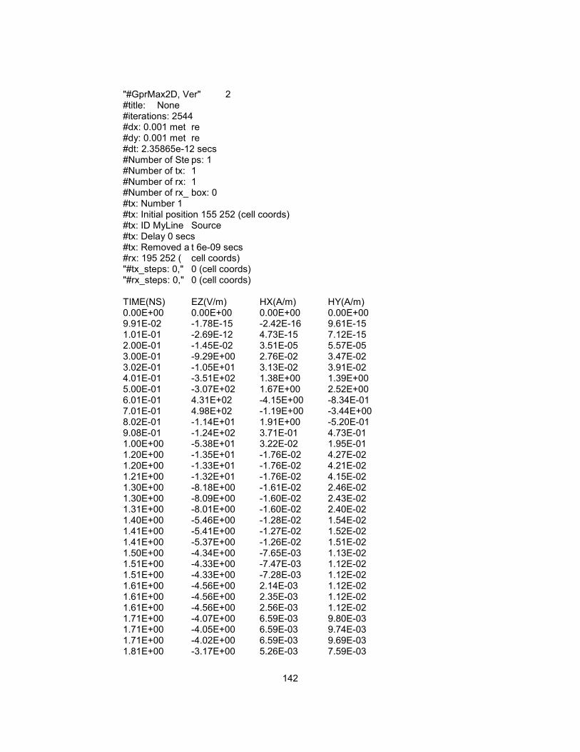
142
"#GprMax2D, Ver" 2 #title: None #iterations: 2544 #dx: 0.001 met re #dy: 0.001 met re #dt: 2.35865e-12 secs #Number of Ste ps: 1 #Number of tx: 1 #Number of rx: 1 #Number of rx_ box: 0 #tx: Number 1 #tx: Initial position 155 252 (cell coords) #tx: ID MyLine Source #tx: Delay 0 secs #tx: Removed a t 6e-09 secs #rx: 195 252 ( cell coords) "#tx_steps: 0," 0 (cell coords) "#rx_steps: 0," 0 (cell coords) TIME(NS) EZ(V/m) HX(A/m) HY(A/m) 0.00E+00 0.00E+00 0.00E+00 0.00E+00 9.91E-02 -1.78E-15 -2.42E-16 9.61E-15 1.01E-01 -2.69E-12 4.73E-15 7.12E-15 2.00E-01 -1.45E-02 3.51E-05 5.57E-05 3.00E-01 -9.29E+00 2.76E-02 3.47E-02 3.02E-01 -1.05E+01 3.13E-02 3.91E-02 4.01E-01 -3.51E+02 1.38E+00 1.39E+00 5.00E-01 -3.07E+02 1.67E+00 2.52E+00 6.01E-01 4.31E+02 -4.15E+00 -8.34E-01 7.01E-01 4.98E+02 -1.19E+00 -3.44E+00 8.02E-01 -1.14E+01 1.91E+00 -5.20E-01 9.08E-01 -1.24E+02 3.71E-01 4.73E-01 1.00E+00 -5.38E+01 3.22E-02 1.95E-01 1.20E+00 -1.35E+01 -1.76E-02 4.27E-02 1.20E+00 -1.33E+01 -1.76E-02 4.21E-02 1.21E+00 -1.32E+01 -1.76E-02 4.15E-02 1.30E+00 -8.18E+00 -1.61E-02 2.46E-02 1.30E+00 -8.09E+00 -1.60E-02 2.43E-02 1.31E+00 -8.01E+00 -1.60E-02 2.40E-02 1.40E+00 -5.46E+00 -1.28E-02 1.54E-02 1.41E+00 -5.41E+00 -1.27E-02 1.52E-02 1.41E+00 -5.37E+00 -1.26E-02 1.51E-02 1.50E+00 -4.34E+00 -7.65E-03 1.13E-02 1.51E+00 -4.33E+00 -7.47E-03 1.12E-02 1.51E+00 -4.33E+00 -7.28E-03 1.12E-02 1.61E+00 -4.56E+00 2.14E-03 1.12E-02 1.61E+00 -4.56E+00 2.35E-03 1.12E-02 1.61E+00 -4.56E+00 2.56E-03 1.12E-02 1.71E+00 -4.07E+00 6.59E-03 9.80E-03 1.71E+00 -4.05E+00 6.59E-03 9.74E-03 1.71E+00 -4.02E+00 6.59E-03 9.69E-03 1.81E+00 -3.17E+00 5.26E-03 7.59E-03

143
1.81E+00 -3.15E+00 5.22E-03 7.55E-03 1.81E+00 -3.13E+00 5.18E-03 7.51E-03 1.91E+00 -1.93E+00 1.82E-03 8.18E-03 1.91E+00 -1.87E+00 1.60E-03 8.33E-03 1.92E+00 -1.81E+00 1.37E-03 8.48E-03 2.01E+00 4.15E+00 -2.51E-02 2.79E-02 2.01E+00 4.35E+00 -2.61E-02 2.87E-02 2.02E+00 4.55E+00 -2.71E-02 2.95E-02 2.11E+00 1.33E+01 -5.58E-02 7.63E-02 2.12E+00 1.36E+01 -5.59E-02 7.80E-02 2.12E+00 1.38E+01 -5.59E-02 7.97E-02 2.21E+00 2.27E+01 6.51E-03 1.45E-01 2.22E+00 2.26E+01 9.41E-03 1.45E-01 2.22E+00 2.26E+01 1.23E-02 1.45E-01 2.32E+00 1.11E+01 4.27E-02 7.45E-02 2.32E+00 1.09E+01 4.06E-02 7.32E-02 2.32E+00 1.08E+01 3.85E-02 7.20E-02 2.42E+00 1.01E+01 -6.07E-03 8.08E-02 2.42E+00 9.73E+00 -3.93E-03 8.07E-02 2.42E+00 9.36E+00 -1.58E-03 8.05E-02 2.52E+00 -1.86E+01 2.40E-01 3.72E-03 2.52E+00 -1.95E+01 2.47E-01 -2.20E-04 2.52E+00 -2.03E+01 2.55E-01 -4.34E-03 2.62E+00 -8.20E+01 2.80E-01 -4.07E-01 2.62E+00 -8.38E+01 2.68E-01 -4.20E-01 2.63E+00 -8.55E+01 2.55E-01 -4.33E-01 2.72E+00 -3.23E+01 -4.59E-01 -2.41E-01 2.72E+00 -2.83E+01 -4.64E-01 -2.18E-01 2.73E+00 -2.43E+01 -4.67E-01 -1.95E-01 2.82E+00 3.98E+01 -3.26E-02 2.31E-01 2.83E+00 3.88E+01 -2.42E-02 2.26E-01 2.83E+00 3.77E+01 -1.64E-02 2.20E-01 2.92E+00 4.89E+00 2.82E-02 3.00E-02 2.93E+00 4.62E+00 2.71E-02 2.83E-02 2.93E+00 4.37E+00 2.61E-02 2.68E-02 3.03E+00 1.01E+00 3.65E-03 5.38E-03 3.03E+00 9.89E-01 3.47E-03 5.24E-03 3.03E+00 9.69E-01 3.30E-03 5.11E-03 3.13E+00 3.57E-02 -1.89E-03 -1.44E-03 3.13E+00 1.88E-02 -2.07E-03 -1.57E-03 3.13E+00 2.89E-03 -2.25E-03 -1.69E-03 3.23E+00 1.12E-01 -5.23E-03 -1.02E-03 3.23E+00 1.15E-01 -5.11E-03 -9.79E-04 3.23E+00 1.17E-01 -4.99E-03 -9.39E-04 3.33E+00 8.28E-02 -2.55E-03 -2.64E-03 3.33E+00 1.05E-01 -2.69E-03 -2.65E-03 3.34E+00 1.30E-01 -2.85E-03 -2.67E-03 3.43E+00 2.04E+00 -1.89E-02 8.82E-05 3.43E+00 2.09E+00 -1.94E-02 2.03E-04 3.44E+00 2.14E+00 -1.99E-02 3.23E-04 3.53E+00 5.40E+00 -3.07E-02 1.63E-02 3.54E+00 5.54E+00 -3.05E-02 1.71E-02

144
3.54E+00 5.67E+00 -3.02E-02 1.79E-02 3.63E+00 6.98E+00 1.45E-02 2.95E-02 3.64E+00 6.81E+00 1.58E-02 2.86E-02 3.64E+00 6.62E+00 1.70E-02 2.76E-02 3.74E+00 -1.18E+00 1.30E-02 -2.07E-02 3.74E+00 -1.22E+00 1.22E-02 -2.11E-02 3.74E+00 -1.25E+00 1.13E-02 -2.14E-02 3.84E+00 1.86E-01 -1.42E-03 -1.33E-02 3.84E+00 2.07E-01 -1.38E-03 -1.32E-02 3.84E+00 2.27E-01 -1.35E-03 -1.30E-02 3.94E+00 4.18E-01 -1.43E-03 -9.92E-03 3.94E+00 4.23E-01 -1.47E-03 -9.84E-03 3.94E+00 4.29E-01 -1.50E-03 -9.76E-03 4.04E+00 8.14E-01 -1.63E-03 -5.45E-03 4.04E+00 8.22E-01 -1.60E-03 -5.35E-03 4.05E+00 8.30E-01 -1.57E-03 -5.26E-03 4.14E+00 1.01E+00 -7.01E-04 -2.54E-03 4.14E+00 1.01E+00 -6.97E-04 -2.48E-03 4.15E+00 1.01E+00 -6.94E-04 -2.43E-03 4.24E+00 1.11E+00 -3.18E-04 -4.31E-04 4.25E+00 1.11E+00 -2.90E-04 -3.94E-04 4.25E+00 1.11E+00 -2.60E-04 -3.58E-04 4.34E+00 9.39E-01 1.73E-03 2.84E-04 4.35E+00 9.33E-01 1.78E-03 2.80E-04 4.35E+00 9.27E-01 1.83E-03 2.75E-04 4.45E+00 5.31E-01 2.91E-03 -1.28E-03 4.45E+00 5.17E-01 2.89E-03 -1.35E-03 4.45E+00 5.03E-01 2.87E-03 -1.42E-03 4.55E+00 3.05E-01 -6.67E-04 -2.43E-03 4.55E+00 3.15E-01 -7.57E-04 -2.36E-03 4.55E+00 3.27E-01 -8.42E-04 -2.28E-03 4.65E+00 4.67E-01 -8.14E-04 1.20E-03 4.65E+00 4.41E-01 -8.13E-04 1.22E-03 4.65E+00 4.14E-01 -8.20E-04 1.24E-03 4.75E+00 -3.51E+00 -1.06E-02 2.08E-03 4.75E+00 -3.69E+00 -1.12E-02 2.15E-03 4.76E+00 -3.88E+00 -1.17E-02 2.23E-03 4.85E+00 -1.22E+01 -3.46E-02 5.50E-03 4.85E+00 -1.22E+01 -3.49E-02 5.52E-03 4.86E+00 -1.23E+01 -3.51E-02 5.54E-03 4.95E+00 -7.05E+00 -2.20E-02 2.31E-03 4.96E+00 -6.81E+00 -2.14E-02 2.18E-03 4.96E+00 -6.56E+00 -2.07E-02 2.06E-03 5.05E+00 1.48E+00 -7.88E-04 -1.98E-03 5.06E+00 1.61E+00 -4.56E-04 -2.04E-03 5.06E+00 1.74E+00 -1.29E-04 -2.10E-03 5.16E+00 4.78E+00 9.00E-03 -2.96E-03 5.16E+00 4.81E+00 9.14E-03 -2.94E-03 5.16E+00 4.84E+00 9.28E-03 -2.92E-03 5.26E+00 5.23E+00 1.20E-02 -3.39E-04 5.26E+00 5.24E+00 1.20E-02 -2.26E-04 5.26E+00 5.24E+00 1.20E-02 -1.09E-04

145
5.36E+00 5.53E+00 1.10E-02 6.98E-03 5.36E+00 5.55E+00 1.10E-02 7.20E-03 5.36E+00 5.56E+00 1.11E-02 7.42E-03 5.46E+00 5.56E+00 1.72E-02 1.46E-02 5.46E+00 5.53E+00 1.75E-02 1.47E-02 5.47E+00 5.50E+00 1.77E-02 1.47E-02 5.56E+00 2.91E+00 2.74E-02 1.03E-02 5.56E+00 2.82E+00 2.75E-02 1.01E-02 5.57E+00 2.72E+00 2.76E-02 9.99E-03 5.66E+00 -1.89E+00 2.87E-02 1.01E-02 5.67E+00 -2.01E+00 2.86E-02 1.03E-02 5.67E+00 -2.13E+00 2.85E-02 1.04E-02 5.76E+00 -5.91E+00 1.73E-02 1.31E-02 5.77E+00 -5.94E+00 1.69E-02 1.30E-02 5.77E+00 -5.98E+00 1.65E-02 1.28E-02 5.87E+00 -5.35E+00 4.33E-03 3.92E-03 5.87E+00 -5.31E+00 4.16E-03 3.68E-03 5.87E+00 -5.27E+00 3.99E-03 3.44E-03 5.97E+00 -3.42E+00 7.96E-04 -4.42E-03 5.97E+00 -3.38E+00 7.73E-04 -4.55E-03 5.97E+00 -3.33E+00 7.50E-04 -4.68E-03

146
Appendix B
MATLAB CODES FOR GPRMAX2D

147
These Matlab codes were generated by Bostanudin, N. (2013) filename = 'beam1.txt; geo = '.geo'; sca = '.sca'; geofile = [filename geo]; scafile = [filename sca]; [mesh,header,media] = gprmax2g(geofile); modeltitle = header.title; dx = header.dx; % cell size in x direction - horizontal for GprMax dy = header.dy; % cell size in y direction - vertical for GprMax nx = header.nx; ny = header.ny; x = nx*dx; y = ny*dy; % Scan data [Header,Fields]=gprmax(scafile); modeltitle = Header.title;
Nsteps = Header.NSteps;
figure(1); imagesc(0:dx:x, 0:dy:y, mesh); set(gca,'YDir','normal') colormap(gray); xlabel('[m]'); ylabel('[m]'); title(modeltitle); % Scan figure(2); imagesc(0:Nsteps, (0:dt:timew)*10^9, ez); % *10^9 to get time in ns colormap(gray); xlabel('Trace no'); ylabel('[ns]'); title(modeltitle); %% Display GPR scan image after mean removal ezmr = mrem(ez); figure(3); imagesc(ezmr); colormap(gray); xlabel('[m]'); ylabel('[ns]'); %

148
References
Ahmad, S. (2003). Reinforcement corrosion in concrete structures, its monitoring and
service life prediction––a review. Cement and Concrete Composites, 25(4), 459-
471.
ASTM C876-09. (2014). Standard test method for half-cell potentials of uncoated
reinforcing steel in concrete. West Conshohocken: American Society for Testing
and Materials.
ASTM WK-37880. (2012). New Test Method for Measuring the Surface Resistivity of
Hardened Concrete Using the Wenner Four-Electrode Method. West
Conshohocken: American Society for Testing and Materials.
Bertolini, L., Bolzoni, F., Pastore, T., & Pedeferri, P. (1996). Behaviour of stainless steel
in simulated concrete pore solution. British Corrosion Journal,31(3), 218-222.
Bostanudin, N. (2013). Computational methods for processing ground penetrating radar
data (Doctoral dissertation, University of Portsmouth).
Chang, C. W., Lin, C. H., & Lien, H. S. (2009). Measurement radius of reinforcing steel
bar in concrete using digital image GPR. Construction and Building
Materials, 23(2), 1057-1063.
Duffó, G., Gaillard, N., Mariscotti, M., & Ruffolo, M. (2015). Application of gamma-ray
radiography and gravimetric measurements after accelerated corrosion tests of
steel embedded in mortar. Cement and Concrete Research,74, 1-9.
Garboczi, E. J., Stutzman, P. E., Wang, S., Martys, N. S., Hassan, A., Duthinh, D., &
Stiles, M. D (2010). Corrosion Detection in Concrete Rebars Using a
Spectroscopic Technique.
Giannopoulos A. (2005) GprMax2D/3D: /http://www.gprmax.orgS.
149
Giannopoulos, A. (1997) The investigation of transmission-line matrix and finite-
difference time-domain methods for the forward problem of ground probing radar.
Ph.D. thesis, University of York, UK.
Giannopoulos, A. (2005). “Modelling ground penetrating radar by GprMax."Construction
and building materials 19.10 (2005): 755-762.
Hong, S., Lai, W. W. L., Wilsch, G., Helmerich, R., Helmerich, R., Günther, T., &
Wiggenhauser, H. (2014). Periodic mapping of reinforcement corrosion in
intrusive chloride contaminated concrete with GPR. Construction and Building
Materials, 66, 671-684.
Hubbard, S. S., Zhang, J., Monteiro, P. J., Peterson, J. E., & Rubin, Y. (2003).
Experimental detection of reinforcing bar corrosion using nondestructive
geophysical techniques. ACI Materials Journal, 100(6).
Kim, S., Surek, J., & Baker-Jarvis, J. (2011). Electromagnetic metrology on concrete and
corrosion. Journal of Research of the National Institute of Standards and
Technology, 116(3), 655-669.
Kunz, K.S., Luebbers RJ (1993). The finite-difference time-domain method for
electromagnetics. Boca Raton: CRC Press.
Lai, W. L., Kind, T., Stoppel, M., & Wiggenhauser, H. (2012). Measurement of
accelerated steel corrosion in concrete using ground-penetrating radar and a
modified half-cell potential method. Journal of Infrastructure Systems, 19(2), 205-
220.Leucci, G. (2012). Ground Penetrating Radar: an Application to Estimate
Volumetric Water Content and Reinforced Bar Diameter in Concrete
Structures.Journal of Advanced Concrete Technology, 10(12), 411-422.
Martino, N., Maser, K., Birken, R., & Wang, M. (2014). Determining Ground Penetrating
Radar Amplitude Thresholds for the Corrosion State of Reinforced Concrete

150
Bridge Decks. Journal of Environmental and Engineering Geophysics,19(3), 175-
181.
Millard, S., & Sadowski, L. (2009). Novel method for linear polarisation resistance
corrosion measurement. e-Journal of Nondestructive Testing & Ultrasonics, 14.
Montgomery, D. C., & Runger, G. C. (2010). Applied statistics and probability for
engineers. John Wiley & Sons.
Parrillo, R., Roberts, R.L., and Haggan, A. (2005) “Bridge Deck Condition Assessment
Using Ground Penetrating Radar”, International Bridge Conference, Pittsburgh,
PA, June 13-15
RADAN 7 (2014 ) [Computer software]. Salem, NH, Geophysical Survey Systems
(GSSI).
Shihab, S., & Al-Nuaimy, W. (2005). Radius estimation for cylindrical objects detected by
ground penetrating radar. Subsurface Sensing Technologies and
Applications, 6(2), 151-166.
Standard, A. S. T. M. (2003). G1-03. Standard Practice for preparing, cleaning, and
evaluating corrosion test specimens, Annual Book of ASTM Standards, 3, 17-25.
Standard, A. S. T. M. (2009). G59–97: Standard Test Method for Conducting
Potentiodynamic Polarization Resistance Measurements. West Conshohocken,
PA: ASTM International.
Taflove, A. (1995). Computational electrodynamics: the finite-difference timedomain
method. Artech House.
The Helpful Engineer (2010), “Carbonation of concrete(corrosion)”
http://thehelpfulengineer.com /index.php/2010/10/carbonation-of-concrete-
corrosion accessed Nov, 2014.

151
Utsi, V., & Utsi, E. (2004, June). Measurement of reinforcement bar depths and
diameters in concrete. In Ground Penetrating Radar, 2004. GPR 2004.
Proceedings of the Tenth International Conference on (pp. 659-662). IEEE.
Washer, G. A. (2013). Concrete reinforcement detection and assessment. The NDT
Technician, 12(2), 1-5.
Yee K. S., (1966),.Numerical Solution of Initial Boundary Value Problems Involving
Maxwell's equations in Isotropic Media., IEEE Transactions on Antennas and
Propagation, Vol. 14, pp. 302-307
Zanzi, L., & Arosio, D. (2013). Sensitivity and accuracy in rebar diameter measurements
from dual-polarized GPR data. Construction and Building Materials, 48, 1293-
1301.
Zhan, B. J., Lai, W. L., Kou, S. C., Poon, C. S., & Tsang, W. F. (2011). Correlation
between accelerated steel corrosion in concrete and ground penetrating radar
parameters. In C. Leung, & K. WAN (Eds.), International RILEM Conference on
Advances in Construction Materials Through Science and Engineering (pp. 563-
571). RILEM Publications SARL.
Zou, X., Schmitt, T., Perloff, D., Wu, N., Yu, T. Y., & Wang, X. (2015). Nondestructive
corrosion detection using fiber optic photoacoustic ultrasound
generator. Measurement, 62, 74-80.

152
Biographical Information
Md Istiaque Hasan has received his BS degree in Civil Engineering from
Bangladesh University of Engineering and Technology. After graduation, he worked as a
site engineer for CESD Consultants in Dhaka, Bangladesh for one year. He graduated
from Louisiana Tech University at Ruston, Louisiana with a MS degree on Civil and
Structural Engineering in 2011. After completing his MS degree, he started his PhD in the
department of Civil Engineering at UT Arlington in 2011. He worked with Dr. Nur Yazdani
as a teaching as research assistant through the duration of his PhD study. His research
interests are non-destructing testing and evaluation, design of reinforced concrete
structures, finite element modeling and retrofitting of old or damaged concrete structures.