Quantitative Methods for Sampling of

Germplasm Collections

Getting the best out of molecular markers when creating

core collections

Thomas L. Odong

ii

Thesis committee

Thesis supervisor

Prof dr. F.A. van Eeuwijk Professor of Applied Statistics Wageningen University

Thesis co-supervisors

Dr.ir. T.J.L. van Hintum Head methodology and documentation, Centre for Genetic Resources, The Netherlands Wageningen UR

Dr.ir. J. Jansen Senior Research Scientist, Biometris Wageningen UR

Other members

Prof. dr. B.J. Zwaan, Wageningen University Dr. J. Engels, Bioversity International, Rome Dr. J.L. Crossa, International Maize and Wheat Improvement Centre (CIMMYT), Mexico Dr. M.J.M. Smulders, Wagenigen UR

This research was conducted under the auspices of the C.T. de Wit Graduate School of Production Ecology and Resource Conservation.

iii

Quantitative Methods for Sampling of

Germplasm Collections

Getting the best out of molecular markers when creating

core collections

Thomas L. Odong

Thesis submitted in fulfillment of the requirements for the degree of doctor

at Wageningen University by the authority of the Rector Magnificus

Prof. dr. M.J. Kropff, in the presence of the

Thesis Committee appointed by the Academic Board to be defended in public

on Wednesday 13 June 2012 at 4 p.m. in the Aula.

iv

Thomas L. Odong Quantitative Methods for Sampling of Germplasm Collections. Getting the best out of molecular markers when creating core collections, 152 pages.

PhD thesis Wageningen University, Wageningen, The Netherlands (2012) With references, with summaries in Dutch and English

ISBN 978-94-6173-209-5

v

To my father, Mr. Kamilo Oyaro Orik (RIP) and my mother Balbina Atyang Oyaro.

Father you always took pride in my academic success, it is a pity that you did not live to

see this day; mum (oma) we are what we are today because of the sacrifices that you

made.

vi

vii

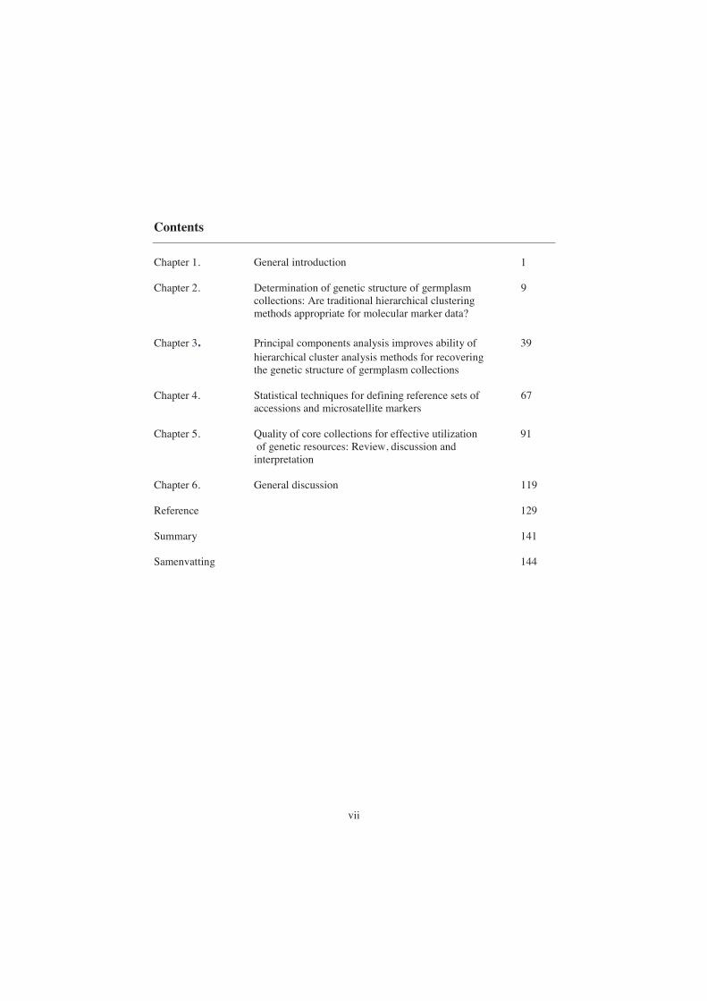
Contents

Chapter 1. General introduction 1

Chapter 2. Determination of genetic structure of germplasm 9 collections: Are traditional hierarchical clustering methods appropriate for molecular marker data?

Chapter 3 Principal components analysis improves ability of 39 hierarchical cluster analysis methods for recovering the genetic structure of germplasm collections

Chapter 4. Statistical techniques for defining reference sets of 67 accessions and microsatellite markers

Chapter 5. Quality of core collections for effective utilization 91 of genetic resources: Review, discussion and interpretation

Chapter 6. General discussion 119

Reference 129

Summary 141

Samenvatting 144

1

Chapter 1

General Introduction

1.1 Background

Ex-situ germplasm collections have increased enormously in number and size over the

last three to four decades as a result of global efforts to conserve plant genetic resources

for food and agriculture. Globally, over seven million accessions of different crop species

are conserved in about 1750 genebanks (Upadhyaya et al. 2010). These accessions are of

a diverse nature and include landraces, selected lines from landraces, elite breeding lines,

released varieties, wild and weedy relatives of cultigens, and genetic stocks from

different areas of origin. Because of this diverse nature, they can provide all relevant

allelic diversity necessary for plant improvement. However, the large sizes of these

collections hinder full exploitation of all available genetic resources. The idea of picking

an accession with genes of interest from say a collection of 80,000 rice accessions is

simply mind boggling for a breeder and this is one of the reasons that the potentials of

plant genetic resources in genebanks have remain largely unexploited. The approach of

forming core collections (core sub-sets) was introduced to ensure efficient and effective

management and utilization of all accumulated plant genetic resources. Frankel (1984)

defined a core collection as a limited set of accessions representing, with minimum

repetitiveness, the genetic diversity of a crop species and its wild relatives. The idea of

core collections is a radical departure from first generation genetic resource conservation

thinking which stresses accumulation without much concern about utilization. From the

original definition, several operational definitions have since been coined (see Brown,

1995; van Hintum et al. 2000).

Core collections have many roles to play in the management and use of genetic resources.

Genebank curators have the responsibility for conservation, regeneration, safety

duplication, documentation, evaluation and characterisation of the genetic resources in

2

their collections. These activities of the genebank often require the curators to make

choices or set priorities among accessions because of limited resources (Brown, 1995).

Because a core collection is smaller in size compared to the whole collection, it enables

some operations of the genebank, such as evaluation, to be handled more efficiently and

effectively. The limited size of a core is key to its manageability, and in many cases the

representation of the collection’s diversity enables the core to function as a reference set

of accessions for the whole collection (Brown and Spillane, 1999). On the other hand,

having a small sample of accessions (core collection) representing the diversity exhibited

by a crop species coupled with evaluation or characterization data would greatly

encourage the breeders to effectively exploit the potential of these genetic resources.

Since the inception of the idea of core collections almost three decades ago, a vast body

of literature on the theory and practice of core collections has accumulated. Very many

approaches for selecting core collections have been proposed and used (e.g. M-Strat

(Gouesnard et al. 2001), Genetic distance sampling (Jansen and van Hintum 2007),

PowerCore (Kim et al. 2007) and Core Hunter (Thachuk et al. 2009)). For several plant

species, core collections have been established using different approaches: sweet potato

(Huaman et al. 1999), maize (Malosetti and Abadie 2001), chickpea (Upadhyaya et al.

2001), peanut (Upadhyaya et al. 2002), rice (Li et al. 2002), soybean (Wang et al. 2006),

bread wheat (Balfourier et al. 2007) and Chilean common bean (Mario et al. 2010).

However, several challenges still exist when it comes to making decisions on

methodologies for selection of core collections.

Designation of a core collection involves a number of decisions especially on quantitative

sampling methodologies. The key issues include amongst others: a) choice of the size of

core collection b) determination of the genetic structure of germplasm collections

(stratification/grouping) c) determination of the number of accession to be selected from

each group d) method to select accessions from the different groups and e) evaluating the

quality of core collections. Each of the key issue mentioned above have received research

attention to a varying degree but a lot still need be done. In the following section we give

3

brief descriptions of the challenges that motivated the different aspects of the research that

led to this thesis.

1.2 Determination of the genetic structure of germplasm collections

Determination of the genetic structure (partitioning) of heterogeneous germplasm

collections is an essential component of the sampling of core collections. Partitioning of

germplasm collections before sampling ensures that both the genetic and the ecological

spectra of germplasm collections are fully represented in core collections (Brown 1995;

van Hintum et al. 2000). In addition, even in cases where core collections were selected

without stratification it may be necessary to associate an accession in the core collection

with accessions in the entire collection; this association can be based on the group

structure of the germplasm collection. The determination of genetic structure is also an

important aspect of association studies (Wang et al. 2005; Shriner et al. 2007); general

agreements exist among researchers that incorporating population structure into statistical

models used in association studies is necessary to avoid false positives (Pritchard et al.

2000b; Flint-Garcia et al. 2003; Zhu et al. 2008).

Whether the genetic structure is needed for use in sampling core collections or for

association studies, an important challenge still is the choice of a method for determining

the genetic structure. In the past, determination of the genetic structure of germplasm

collections has mainly been done using passport data (van Hintum 2000) or multivariate

statistical methods such as cluster analysis, principal component analysis, and

multidimensional scaling, usually based on agronomic data (Peeters and Martinelli 1989;

Franco et al. 1997, 2005, 2006). However, in recent years, many new methods have been

developed especially for studying the genetic structure of natural populations using

molecular markers, e.g. STRUCTURE (Pritchard et al. 2000), PCA (Patterson et al.

2006) and PCO-MC (Reeves and Richards 2009). Despite the introduction of these

approaches, most researchers in the plant sciences still use traditional methods especially

hierarchical clustering techniques for studying genetic diversity in crop species (see

Folkertsma et al. 2005; Perumal et al. 2007; Barro-Kondombo et al. 2010; D'hoop et al.

4

2010). The popularity of traditional hierarchical clustering techniques such as Ward’s

method stems from the fact that they a) require little computer time compared to other

methods, b) are available in many general statistical packages, c) are frequently used in

different types of applications and d) the output is easy to interpret. Moreover, traditional

hierarchical clustering techniques do not require genetic assumptions such as Hardy-

Weinberg or linkage equilibrium. However, with the changes in types, quality and

quantity of data used for studying genetic structure of germplasm collections, the

performance of traditional hierarchical clustering techniques ought to be evaluated. For

example, most evaluations of the performance of hierarchical clustering methods were

based on data sets of very limited sizes (Milligan and Cooper 1985). In addition, most

studies carried out to evaluate the performance of hierarchical clustering methods with

respect to germplasm collections were not carried out molecular marker data (Peeters and

Martinelli, 1989; Franco et al. 1997, 2005, 2006). Currently, we are not aware of any

study in which the performance of hierarchical clustering techniques was evaluated

specifically using molecular marker data. With the expected reduction in the cost of

genotyping, researchers will be faced with datasets of thousands of accessions genotyped

with many molecular markers so there is strong need to evaluate the performance of the

traditional hierarchical clustering techniques using large sets of molecular marker data. In

general it is not clear how traditional clustering will perform under different factors

affecting genetic diversity like migration and reproductive system of the materials that

constitute germplasm collections. The response received on a recent paper (Odong et al.

2011; Chapter 2) on cluster analysis using molecular markers is a good indication of the

growing interest of researchers in this topic. This paper was consistently the most

downloaded paper from Theoretical and Applied Genetics for a period seven months

(April - November 2011) with over 300 downloads per month. In addition, it has been

suggested in the literature (Patterson et al. 2006) that the use of principal component

analysis (PCA) could boost the performance the traditional clustering technique for

determining the population genetic structures. The integration of PCA and cluster

analysis is likely to contribute tremendously to improving the ability of the traditional

cluster analysis when determining the genetic structure of germplasm collections

(Chapter 3).

5

1.3 Connecting germplasm collections in different genebanks : Reference sets of

accessions and molecular markers

The exploitation of the full potential of plant genetic resources cannot be complete

without linking information on genetic diversity from the different germplasm collections

(genebanks) around the world. It is possible to establish relations between genebank

collections by defining for each crop a small but informative set of accessions, together

with a small set of reliable molecular markers, that can be used as reference material

(reference sets). The reference material should be an adequate representation of the

genetic diversity of that crop as stored in genebanks around the world. In that case,

molecular marker information can be used to place new accessions in the spectrum of

current accessions. The designation of reference sets will help in the identification of

overlaps between germplasm collections and this will allow these collections to be

analyzed together thus enlarging the space of our inference. The reference sets can also

be used to connect different population genetic and quantitative genetic studies, including

association studies. However, defining statistical methods for selecting such a

representative subsets of accessions and molecular markers is a challenge. The

Generation Challenge Programme –CGP (GCP; http://www.generationcp.org) initiated

the process of constructing reference sets by genotyping large numbers of accessions of

important agricultural crops using microsatellite markers.

For the selection of such a representative subset of accessions, the ideal method should be

based on the relationship between the selected accessions (entries) and the accessions not

selected in the subset. Most existing algorithms for selection of core collection

(MSTRAT (Gouesnard et al. 2001), PowerCore (Kim et al. 2007) and Core Hunter

(Thachuk et al. 2009)) pay more attention to the content of the core collections but tend to

ignore the relationships between the selected entries and those accessions not included in

the subset. In addition, by aiming at maximizing genetic diversity parameters such as

allelic richness, average distances between selected accessions, methods such as

MSTRAT (Gouesnard et al. 2001) are likely to select mainly non-representative

6

accessions (“outliers”). In other words, none of the existing algorithms for selecting core

collections was developed to select accessions to serve as representatives around which

the other accessions can be positioned.

For the selection of a subset of molecular markers, the aim is to obtain a subset of

markers that would preserve the major population genetic structure in the data. Currently

the most common criterion used for selection of molecular markers in plant germplasm

studies is the polymorphic information content – PIC (Botstein et al. 1980). It should be

noted that PIC favors molecular markers with very many alleles of equal frequencies.

Although molecular markers with high PIC may be good for differentiating between

individual accessions, those markers are likely to perform poorly with respect to detecting

differences between groups (population structure). In addition, two markers with high

PIC may contain similar information and thus introduce redundancy in the subset of

selected markers. Consequently, there is a need to come up with methods for the

selection of subsets of molecular markers which describe the major genetic structure in

the data with minimum redundancy.

1.4 Quality criteria for evaluation of core collection

When comparing the options for assembling core collections, one of the challenges is to

choose the right evaluation criteria for gauging the quality of the result. Various criteria

for determining the suitability of a core collection have been suggested in the literature,

yet very little attention has been given to the analysis of these quality criteria. In fact most

researchers appear to choose quality evaluation criteria simply because they were used in

earlier publications. There is a need to clearly define criteria for the evaluation of the

quality of core collections and to determine the conditions under which these criteria are

suitable. For example, a core subset formed for the purpose of capturing rare or extreme

traits (e.g. high resistance to pest or high yield) should be evaluated differently from one

formed with the intention of representing the pattern of genetic diversity in the collection.

7

1.5 Study objectives and outline of the thesis

The work in this thesis aims at improving knowledge associated with the sampling of

core collections and the roles that core collections have to play in the utilization of plant

genetic resources. This thesis looked at three key aspects of core collection development

and its roles in utilization of plant genetic resources: a) determination of the genetic

structure of germplasm collections and the relevance of the genetic structure in core

selection and utilization of germplasm resources in general b) creating links between

genetic resources stored in different parts of the world and c) critical examination of

criteria for evaluating the quality of core collections.

In chapter 2 we study the appropriateness of traditional hierarchical clustering techniques

(Ward’s method and UPGMA) for determining the structure of germplasm collections

using molecular marker data. The relationships between criteria used for evaluating the

output of cluster analysis (co-phenetic correlation coefficient and agglomerative

coefficient) and population genetic structure parameters (F-statistic) will be explored.

The performance of hierarchical clustering techniques will be compared amongst

themselves and with STRUCTURE (Pritchard et al. 2000). STRUCTURE is a computer

program especially developed for studying the population structure of natural

populations. Real and simulated data sets were used in the study.

Chapter 3 we look at the possibilities of using principal component analysis (PCA) to

boost the performance of traditional hierarchical clustering techniques for determining

the genetic structure of germplasm collections. In this chapter we will study the ability of

the Tracy-Widom distribution to accurately determine the number of genetically

differentiated groups in germplasm collections. The significant principal components

(PCs) based on the Tracy-Widom distribution will be used for the grouping of accessions

usinga traditional hierarchical clustering technique (Ward’s method) and a model-based

clustering method (Mclust). The performance of Ward’s clustering technique using

Euclidean distance based on significant PCs (reduced data set) will be compared with

clustering based on several other distances measures calculated using the full data set.

8

In chapter 4 we propose and discuss several statistical techniques for defining a

representative subset of accessions and molecular markers that can be used for

connecting genetic resources in different genebanks. We will study Genetic Distance

Optimization (GDOpt) as a suitable method for the selection of a representative set of

accessions. For the selection of molecular markers we will evaluate backward elimination

methods as well as methods based on principal component analysis. The current practice

of using the polymorphic information content (PIC) as a criterion for selecting molecular

markers will be used as a baseline against which the other methods will be compared.

Chapter 5 we critically examine criteria for quality evaluation of core collections. We

will define different types of core collections and relate each type of core collection with

suitable quality evaluation criteria. We propose distance-based evaluation criteria and

evaluated their performance using real data sets.

Finally chapter 6 provide a general discussion and draw conclusions.

T.L. Odong • J. van Heerwaarden • J. Jansen • Th.J.L. van Hintum • F.A. van Eeuwijk (2011) Determination of genetic structure of germplasm collections: Are traditional hierarchical clustering methods appropriate for molecular marker data? Theor Appl Genet 123(2):195-205: doi 10.1007/s00122-011-1576-x

Chapter 2

Determination of genetic structure of germplasm collections: Are traditional

hierarchical clustering methods appropriate for molecular marker data?

Abstract

Despite the availability of newer approaches, traditional hierarchical clustering remains

very popular in genetic diversity studies in plants. However, little is known about its

suitability for molecular marker data. We studied the performance of traditional

hierarchical clustering techniques using real and simulated molecular marker data. Our

study also compared the performance of traditional hierarchical clustering with model-

based clustering (STRUCTURE). We showed that the co-phenetic correlation coefficient

is directly related to subgroup differentiation and can thus be used as an indicator of the

presence of genetically distinct subgroups in germplasm collections. Whereas UPGMA

performed well in preserving distances between accessions, Ward excelled in recovering

groups. Our results also showed a close similarity between clusters obtained by Ward and

by STRUCTURE. Traditional cluster analysis can provide an easy and effective way of

determining structure in germplasm collections using molecular marker data, and, the

output can be used for sampling core collections or for association studies.

10

2.1 Introduction

Information about the structure of germplasm collections is of great importance for both

the conservation and utilization of genetic resources collected in genebanks. Because of

the diverse nature of genebank germplasm materials (landraces, selected lines from

landraces, elite breeding lines, released varieties, wild and weedy relatives of the

cultigen, and genetic stocks from different areas of origin), they provide all relevant

allelic diversity necessary for plant improvement. These materials are therefore very

suitable for example for association studies (D’hoop et al. 2010). However, the large

numbers of accessions accumulated in genebanks reduce the efficiency and effectiveness

with which these genetic resources can be exploited. The approach of forming core

collections (core sub-sets) was introduced to solve the above problem. Frankel (1984)

defined a core collection as a limited set of accessions representing, with minimum

repetitiveness, the genetic diversity of a crop species and its wild relatives.

Determination of the genetic structure (partitioning) of heterogeneous germplasm

collections is an essential component in the sampling of core collections since

partitioning of germplasm collections before sampling ensures that both the genetic and

the ecological spectra of germplasm collections are fully represented in core collections

(Brown 1995; van Hintum et al. 2000). In addition, it may be necessary to associate a

accessions in the core collection with the entire collection; the association can be based

on the group structure.

The determination of genetic structures of germplasm collections is also an important

aspect of association studies (Wang et al. 2005; Shriner et al. 2007). General agreement

exist among researchers that incorporating population structure into statistical models

used in association mapping is necessary to avoid false positives (Pritchard et al. 2000b;

Flint-Garcia et al. 2003; Zhu et al. 2008). The general model for association mapping can

be written as “phenotype = marker + genotype + error”, and test for a marker effect is

equivalent to testing for a QTL. Typically genotype is a random factor whose effects are

structured by kinship or population structure. This simple model can be improved by

incorporating information on the relationships between the genotypes a.k.a. population

11

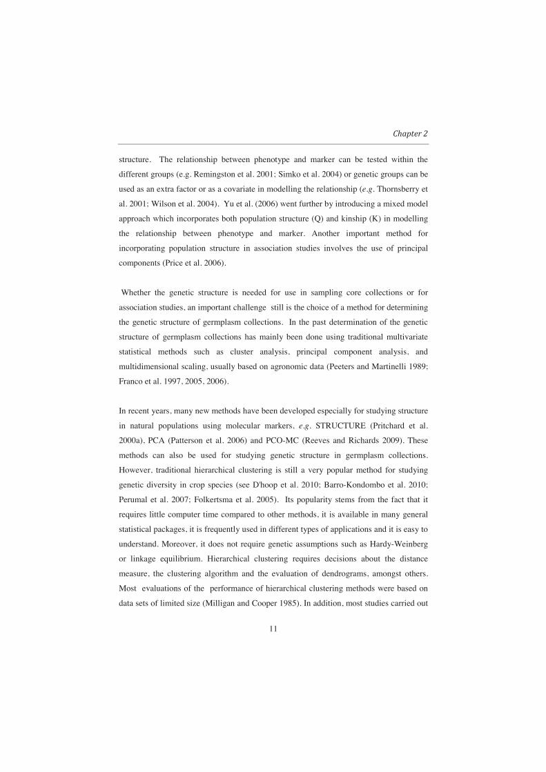
structure. The relationship between phenotype and marker can be tested within the

different groups (e.g. Remingston et al. 2001; Simko et al. 2004) or genetic groups can be

used as an extra factor or as a covariate in modelling the relationship (e.g. Thornsberry et

al. 2001; Wilson et al. 2004). Yu et al. (2006) went further by introducing a mixed model

approach which incorporates both population structure (Q) and kinship (K) in modelling

the relationship between phenotype and marker. Another important method for

incorporating population structure in association studies involves the use of principal

components (Price et al. 2006).

Whether the genetic structure is needed for use in sampling core collections or for

association studies, an important challenge still is the choice of a method for determining

the genetic structure of germplasm collections. In the past determination of the genetic

structure of germplasm collections has mainly been done using traditional multivariate

statistical methods such as cluster analysis, principal component analysis, and

multidimensional scaling, usually based on agronomic data (Peeters and Martinelli 1989;

Franco et al. 1997, 2005, 2006).

In recent years, many new methods have been developed especially for studying structure

in natural populations using molecular markers, e.g. STRUCTURE (Pritchard et al.

2000a), PCA (Patterson et al. 2006) and PCO-MC (Reeves and Richards 2009). These

methods can also be used for studying genetic structure in germplasm collections.

However, traditional hierarchical clustering is still a very popular method for studying

genetic diversity in crop species (see D'hoop et al. 2010; Barro-Kondombo et al. 2010;

Perumal et al. 2007; Folkertsma et al. 2005). Its popularity stems from the fact that it

requires little computer time compared to other methods, it is available in many general

statistical packages, it is frequently used in different types of applications and it is easy to

understand. Moreover, it does not require genetic assumptions such as Hardy-Weinberg

or linkage equilibrium. Hierarchical clustering requires decisions about the distance

measure, the clustering algorithm and the evaluation of dendrograms, amongst others.

Most evaluations of the performance of hierarchical clustering methods were based on

data sets of limited size (Milligan and Cooper 1985). In addition, most studies carried out

12

to evaluate the performance of hierarchical clustering methods with respect to germplasm

collections were on non-molecular marker data (Peeters and Martinelli, 1989; Franco et

al. 1997, 2005, 2006). We are not aware of any study in which the performance of

hierarchical clustering techniques were evaluated specifically using molecular marker

data. With the expected reduction in the cost of genotyping, we will be faced with

datasets of thousands of accessions genotyped with several molecular markers so there is

strong need to evaluate the performance of the traditional hierarchical clustering

techniques using large sets of molecular marker data. The structure of genetic diversity in

germplasm collections is totally different compared to natural populations. It is not clear

how traditional clustering will perform under different factors affecting genetic diversity

like migration and reproductive system of the materials that constitute germplasm

collections. As pointed out by Mohammadi (2003), very few studies in plant genetic

diversity have critically analyzed the performance of different clustering procedures

especially with respect to molecular markers.

Several methods for evaluating the results of hierarchical clustering techniques exist.

When performing hierarchical cluster analysis, we are interested in answering some of

the following questions: 1) is there agreement between the original distances and the

distances between individuals as represented by the dendrogram 2) what can the

dendogram tell us about structure in the data set and 3) what is the optimum number of

clusters for a given data set? One of the most popular measures of agreement between

the original distances and the distances in dendrogram is the co-phenetic correlation

coefficient (CPCC) (Sokal and Rohlf 1962); another measure is the stress criterion of

Kruskal (1964). Only a few measures for the presence of hierarchical structure can be

found in the literature. Kaufman and Rousseeuw (1990) proposed the agglomerative

coefficient (AC) as a criterion for measuring the amount of hierarchical structure in the

data. A large number of methods have been proposed to deal with the optimum-number-

of-clusters problem. A classical study is that of Milligan and Cooper (1985) who

examined the performance of 30 of such criteria. Since then many criteria for determining

the optimal number of clusters were introduced: the silhouette statistic (Rousseeuw

1987), Krzanowski and Lai’s index (Krzanowski and Lai 1988), the gap method

13

(Tibshirani and Walther 2001), the Clest method (Dudoit and Fridlyand 2002), the jump

method (Sugar and James 2003) and the weighted gap method (Yan and Ye 2007). In

general, little attention has been paid to the behaviour of the above measures and methods

in relation to molecular marker data from germplasm collections. A literature search

indicated that so far no study tried to relate the amount of genetic structure in a

germplasm collections to the performance of hierarchical cluster analysis techniques. The

main objective of our study is to determine a relationship between dendogram evaluation

criteria such as CPCC, AC to subgroup differentiation (genetic structure). In addition, we

also compared the performance of hierarchical clustering techniques with model-based

clustering methods.

In this paper, the merits of hierarchical clustering techniques for application in

germplasm collections will be considered. The materials and methods section contains a

brief description and overview of clustering techniques, the evaluation criteria and the

methods used for generating simulated data. The real data set used for illustration in this

paper is also described. In the results section, we present results of cluster analysis of

both real and simulated data sets. We compare the results of two traditional hierarchical

clustering techniques (UPGMA and Ward) with the model-based cluster analysis

program STRUCTURE (Pritchard et al. 2000a), and show using simulated data how

different evaluation criteria of hierarchical cluster analysis are related to subpopulation

differentiation.

14

2.2 Material and Methods

2.2.1 Motivation of the study

This study was motivated by the need to study genetic diversity of several important food

crops under the Generation Challenge Programme-GCP (www.generationcp.org). The

Generation Challenge Programme is a broad network of partners from international

agricultural research institutes and national agricultural research programs collectively

working to improve crop productivity in the developing world, especially environments

prone to drought, low soil fertility, pests and diseases. All the real data sets used in this

study were generated under GCP subprogram I – Crop Genetic Diversity.

2.2.2 Data

Real data: The real data that will be used to illustrate methods consist of 1014 accessions

of coconut (Cocos nucifera) genotyped with 30 SSR markers. The accessions were

collected from different regions of the world: West Africa (32), North America (52),

South Asia (62), Latin America (72), Central America & the Caribbean (109), East Africa

(124), South East Asia (183) and the Pacific Islands (380). Coconut is a diploid, mainly

out-crossing species. Most of the accessions in this collection were indicated as tall; 43

dwarf accessions were present mainly from South East Asia. Dwarf coconuts have a high

degree of self-fertilization. Because of its usefulness, coconut has been extensively

distributed around the world. For this study, the coconut data were selected because it

contained larger numbers of accessions of each of the diverse origins (a typical genebank

germplasm collection).

Two additional data sets, on potato (Solanum species) and common bean (Phaseolus

vulgaris), are described, analyzed and discussed in Appendix 1. The potato data (233

accessions; 50 SSR markers) contained several unique accessions which act like outliers.

All accessions used in this study are diploid. Unlike coconut and potato, common bean is

a predominantly selfing species. The common bean data (603 accessions; 36 SSR

markers) consist of accessions of two distinct types, Mesoamerican and Andean.

Simulated data Marker data were simulated by SimuPOP (Peng and Kimmel

2005), a forward-time population genetic simulation environment. We used a finite

15

island (Wright, 1931) and a stepping stone (Kimura, 1953) migration models. In each

generation, random mating (with 2% selfing) was assumed to produce a diploid genotype

for 30 unlinked loci for each individual, which had a certain probability of migrating to

another subpopulation. We simulated 1000 individuals in five subpopulations of varying

subpopulation differentiation levels (differentiation between subpopulations was

determined by migration rates and number of generations). The migration rates used in

this study were 0, 1 and 2 migrants per subpopulation. At each of the 30 loci, the average

allele frequency of coconut data was used as the starting allele frequency for the

simulation. Within each parameter set, all the loci had the same mutation dynamics,

which occurs according to a K-allele model (KAM). Under the KAM model, there are K

possible allelic states, and any allele has a constant probability of mutating into any of the

other K–1 allelic states (Crow and Kimura 1970). A mutation rate of 2 x 10-5 with 50

possible allelic states was used in the simulation. The mutation parameters were set to

mimic highly polymorphic markers such as SSR markers. However, in this case the role

of mutation is very limited since we used a limited number of generations in the

simulation. In addition to using alleles from real data as starting frequencies for

simulation, the numbers of generations for the simulations were restricted (from 5 to 200

generations) to mimic the situation of agricultural crops in the genebanks.

2.2.3 Distance

In this paper, we used genetic distances (D) based on the proportion of shared alleles

(PSA) where

D = 1 - PSA, and

MffPSA ma

M

m

A

ama

m

/),min( 21 1

1== =

,

where in diploids maf 1 and maf 2 are the frequencies of allele a ( a =1, 2… mA ; mA is the

total number of alleles for molecular marker m ( m =1, 2… M )) in individuals 1 and 2,

respectively, and 1or0 21

21 ,f,f mama = . For more information on the proportion of shared

alleles as similarity measure, see Bowcock et al. (1994), Chakraborty and Jin (1994) and

16

Chang et al. (2009). The effect of distance measures on the grouping of accessions will be

considered in another paper.

2.2.4 Clustering Techniques

Hierarchical clustering techniques From the literature on determination of the

structure of plant germplasm collections, the most popular clustering methods are

Unweighted Pair Group Method with Arithmetic Mean (UPGMA; (Sokal and Michener

1958)) and Ward’s method (Ward 1963). For the purpose of this study, only these two

hierarchical clustering methods (hereafter referred to as UPGMA and Ward) will be

discussed; both methods are well described in Kaufman and Rousseeuw (1990) and

Johnson and Wichern (2002).

The differences between hierarchical clustering algorithms lie mainly in how the

distances between pairs of objects or clusters are defined. In UPGMA the distance

between two clusters is defined as the unweighted mean of the distances between all pairs

of accessions, one from each cluster. At each step, the two nearest clusters are joined.

Ward employs analysis of variance (ANOVA) approach for calculating the distances

between clusters. For each pair of clusters, the sum of squared deviations between each

accession and the centre of the new cluster (error sum of squares) is calculated and the

pair of clusters that yields the lowest error sum of squares are merged. In other words at

each step in the clustering process, the effect of the union of every possible pair of

clusters is considered, and the two clusters that produce the smallest increase in error sum

of squares are joined. It should be noted that both UPGMA and Ward use Lance and

William’s recurrence formula (Lance and Williams 1967) to operate directly on any

distance matrix.

Model-based clustering techniques The most popular model-based clustering

technique is STRUCTURE (Pritchard et al. 2000a; Falush et al. 2003, 2007).

STRUCTURE assumes a model with K populations; K may be unknown. It is assumed

17

that within populations loci are in linkage equilibrium and Hardy-Weinberg equilibrium;

STRUCTURE assigns individuals to populations to achieve this.

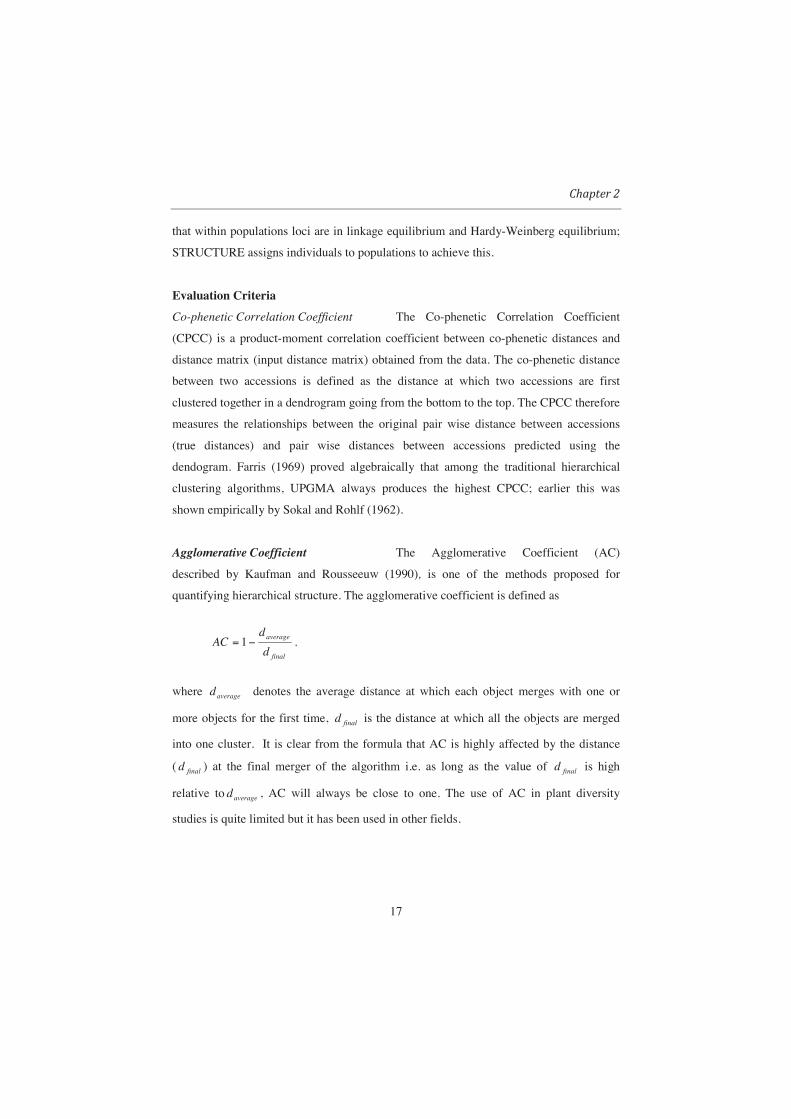
Evaluation Criteria

Co-phenetic Correlation Coefficient The Co-phenetic Correlation Coefficient

(CPCC) is a product-moment correlation coefficient between co-phenetic distances and

distance matrix (input distance matrix) obtained from the data. The co-phenetic distance

between two accessions is defined as the distance at which two accessions are first

clustered together in a dendrogram going from the bottom to the top. The CPCC therefore

measures the relationships between the original pair wise distance between accessions

(true distances) and pair wise distances between accessions predicted using the

dendogram. Farris (1969) proved algebraically that among the traditional hierarchical

clustering algorithms, UPGMA always produces the highest CPCC; earlier this was

shown empirically by Sokal and Rohlf (1962).

Agglomerative Coefficient The Agglomerative Coefficient (AC)

described by Kaufman and Rousseeuw (1990), is one of the methods proposed for

quantifying hierarchical structure. The agglomerative coefficient is defined as

final

average

d

dAC = 1 ,

where averaged denotes the average distance at which each object merges with one or

more objects for the first time, finald is the distance at which all the objects are merged

into one cluster. It is clear from the formula that AC is highly affected by the distance

( finald ) at the final merger of the algorithm i.e. as long as the value of finald is high

relative to averaged , AC will always be close to one. The use of AC in plant diversity

studies is quite limited but it has been used in other fields.

18

Determining the optimal number of clusters

Milligan and Cooper (1985) evaluated 30 rules for determining the optimal number of

clusters. For illustration, one of the best six methods according to Milligan and Cooper

(1985), the point biserial correlation, will be compared with the average silhouette

coefficient proposed by Rousseew (1987). The two criteria were chosen because of their

easy interpretation. The Point-Biserial Correlation (PBC) (Milligan 1981) is defined as

the correlation between corresponding entries in the original distance matrix and a matrix

consisting of zeros and ones indicating whether two objects are in the same cluster or not.

This is an easy measure of the resemblance between the distance matrix and the resulting

tree.

The Average Silhouette Coefficient (ASC) (Rousseeuw 1987) combines the concepts of

cluster cohesion and separation; it relates distances between objects within the same

cluster with distances between objects in different clusters. The silhouette coefficient ( s )

of an object is calculated as:

),max(/)( ababs = , where a is the average distance of an object to all the objects in

the same cluster and b is the minimum average distance between an object to objects in

any of the other clusters.

The average silhouette coefficient for each cluster is calculated by averaging the

silhouette coefficients of all the objects in the cluster. An overall measure of the quality

of the clustering is obtained by computing the average silhouette coefficient over of all

objects in the data. Two other criteria (C-Index (Hubert, 1976) and method based on FST)

for determining the optimum number of clusters are discussed in Appendices 2. In

applying the criteria for determining optimum numbers of clusters, each dendrogram was

cut into a specified number of clusters K( = 2, 3 … 10) and values of the criteria for

determining the number of clusters were calculated and plotted against K. For both PBC

and ASC, the number of clusters (K) at which the plot of K versus the value of the

criterion is maximum is considered as the optimum number of cluster for a given data

set. It should be noted that all these criteria do not directly test for the presence of one

cluster (K =1).

19

2.2.5 Data analysis

Real data. After performing cluster analysis using UPGMA and Ward,

CPCC and AC were calculated. The results from hierarchical cluster analysis were also

compared with the results from STRUCTURE with regard to cluster composition and

appropriate number of clusters.

STRUCTURE was run under the assumption of an admixture model with independent

allele frequency model. No prior information was used. Calculations were carried with

the number of subgroups K ranging from two to 10 with three independent repeats for

each K and with 100,000 iterations of which the first 30,000 were used as burn-in.

Simulated data In this paper the analysis of variance (ANOVA) approach

(algorithm described by (Yang 1998)) and implemented in Hierfstat package in R by

(Goudet 2005) was used to calculate subgroup differentiation (FST). To explore the

relationships between FST and clustering evaluation criteria, datasets from different

simulations were pooled together and then grouped based on the strength of subgroup

differentiation into groups (each containing 100 datasets) with similar realized values of

FST. Hierarchical cluster analysis was performed using Agglomerative Nesting (Agnes)

procedure (Kaufman and Rousseeuw 1990) of the package Cluster of R.

The ability of UPGMA and Ward to recover the subpopulations in the simulated data was

evaluated using overall cluster purity (Zhao and Karypis 2004). Overall purity was

calculated as follows. Let i

ijij m

mp = be the probability that a member of cluster i (i =

1,2,…, I) belongs in reality to subpopulation j (j = 1, 2,…., J), ijm is the number of

members of subpopulation j allocated to cluster i and im is the number of members of

cluster i . The purity for each cluster ( ip ) is defined as the maximum probability of

correct assignment of cluster i to one of the subpopulations, i.e. ( ),pmaxp ijj

i = and over

all purity is defined as =

k

ii

i pm

m

1

.

20

2.3 Results

2.3.1 Coconut

Both dendrograms (UPGMA and Ward) resulted into two major clusters (Fig 1), but

clear differences were evident within these clusters. For example, any attempt to produce

more than two clusters from each dendogram result into groups of very different

structures with UPGMA resulting into highly unbalanced clusters in terms of sizes,

(many of the clusters contained one or two accessions) compared to Ward. UPGMA

(CPCC = 0.82) preserved the original distance matrix better than Ward (CPCC = 0.74).

The two dendrograms had very different values of AC (Ward: 0.97; UPGMA: 0.58).

Fig 1: Dendrograms for the coconut data a) Ward; b) UPGMA. Dendrograms produced by Ward and UPGMA are clearly different with respect to branching. Ward dendrogram had Cophenetic Correlation Coefficient (CPCC) of 0.74 and Agglomerative Coefficient (AC) of 0.97 while UPGMA had CPCC of 0.82 and AC of 0.58. The two major clusters in the two dendrograms had similar compositions (Accessions associated with Indian and Atlantic Oceans versus those associated with the Pacific Ocean)

a) b)

21

When applied to the Ward dendogram, both criteria for determining the optimum number

of clusters (PBC and ASC) identified two as the optimal number of clusters for the

coconut data (Fig 2 a) and b)). However, when applied to UPGMA dendrogram, PBC

was not able to identify an optimum number of clusters i.e. changing the number clusters

from two to ten produced very similar correlations (Fig 2 a). STRUCTURE (method by

Evanno et al. 2005) also showed two as the optimum number of clusters (see Appendix

1).

Fig 2: a) Plot of the Point-Biserial Correlation (PBC) versus the number of groups for the UPGMA and Ward dendograms for the coconut data. b) Plot of the Average Silhouette Coefficient (ASC) versus the number of groups for the UPGMA and Ward dendograms for the coconut data. For both criteria, the number of groups (K) for which the criterion is maximum (or point where the plot flattens off) indicates the optimum number of clusters. Both criteria show two as the optimum number of clusters

Composition of clusters

The two major groups identified by both UPGMA and Ward contained accessions

associated with the Pacific Ocean versus accessions associated with the Atlantic and

Indian oceans. These two major groups were also observed when clustering was done

using STRUCTURE (K=2) (see Fig 3). While further subdivision obtained from Ward’s

dendogram led to formation of clusters/groups which coincided with groups based on

22

passport data (region of origin), this was not possible with UPGMA. In terms of

grouping of accessions, the results from STRUCTURE are quite similar to those of Ward.

In fact, for the number of groups (K) equal two, three or four, the groups formed by

STRUCTURE were almost identical to those produced by cutting Ward’s tree to produce

the same number of clusters (Fig 3). For example, by specifying (K = 3), both

STRUCTURE and Ward resulted into the following three groups: 1) accessions

associated with the Atlantic and Indian oceans 2) accessions from Central America

(Panama) and 3) other accessions associated with the Pacific ocean. Similarity between

groups formed by STRUCTURE and Ward was also observed for the potato data (see

Appendix 1).

2.3.2 Simulated data

The two migration models (Island and Stepping stone) yielded identical results so only

the results of the Island model will be shown. The simulated data sets varied greatly with

respect to subpopulation differentiation with realized FST ranging from 0.010 to 0.431. In

general, the values of CPCC increased with subgroup differentiation (expressed as FST);

UPGMA produced a consistently higher CPCC than Ward (Fig. 4). The difference in

CPCC between UPGMA and Ward decreased with increasing subgroup differentiation.

AC also increased with subpopulation differentiation for both UPGMA and Ward (Fig.

4). In this case Ward showed a higher AC than UPGMA; Ward reached the maximum

value of one with FST just over 0.1, i.e. the curve flattens off much quickly.

23

Fig 3: A) Bar plots for individual coconut accessions generated by cutting the Ward dendogram into a specified number of clusters/groups; the numbers of clusters from top to bottom were 2, 3, 4 and 5. The clusters are represented by different colours. Each column represents one accession. The labels below the bar plots indicate the regions of origin of the coconut accessions. B) Bar plots for individual coconut accessions generated by STRUCTURE 2.2 using the admixture model with independent allele frequency model based on 30 SSR markers; the numbers of clusters from top to bottom were 2, 3, 4 and 5. The groups are represented by different colours. Each bar is partitioned into segments indicating its genetic composition, the longer the segment the more an accession resembles one of the groups. The labels below the bar plots indicate the regions of origin of accessions.

24

Fig 4: A) Relationship between Cophenetic Correlation Coefficient (CPCC) and subgroup differentiation (FST) for the simulated data A) Relationship between Agglomerative Coefficient (AC) and subgroup differentiation (FST) for the simulated data. Each data point is the average of 100 datasets with similar subgroup differentiation.

Identification of the optimum number of groups

Cutting of UPGMA trees resulted into highly unbalanced clusters (one or two clusters

containing the majority of accessions with several other clusters with 1 or 2 accessions

like in real data); only results for Ward is presented. The performance of the criteria for

determining optimum number of clusters also depended on the amount of subgroup

differentiation (Fig. 5). With relatively weak population differentiations (FST <0.08), all

methods performed quite poorly in identifying the correct number of groups. At low

differentiation levels, most criteria for determining optimum number of clusters gave two

as the appropriate number of clusters. We also noticed that for a number of data sets

with weak subgroup differentiations the values of criteria for determining optimum

number of clusters either kept rising or falling, or kept fluctuating to an extent which did

not allow determination of an optimum number of clusters. At higher levels of

population differentiation (FST > 0.2) the performances of became similar.

25

Fig 5: Percentages of simulated data sets for which the Point Biserial Correlation (PBC) and the Average Silhouette Coefficient (AC) identified the correct number of clusters versus the subgroup differentation (FST) (results from Ward only). Each point is based on 30 simulated data sets.

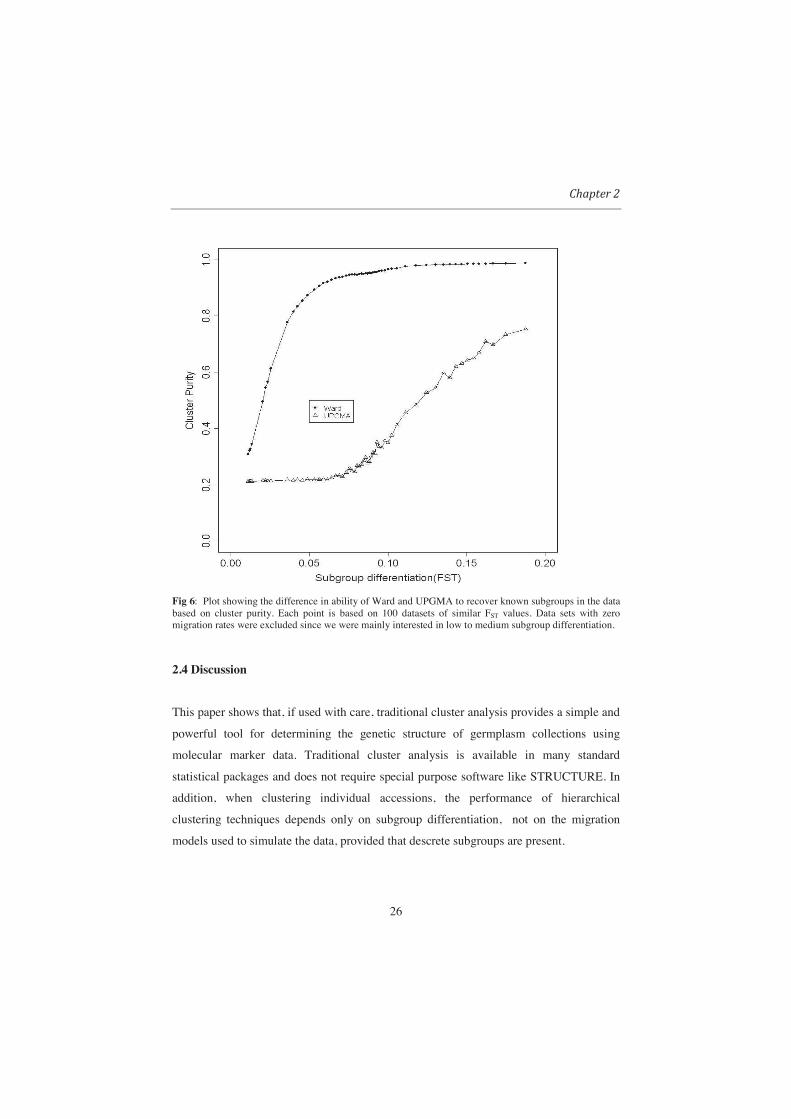
From Fig 6 it can be observed that Ward performed well in recovering the

subpopulations. Except for relatively weak subpopulation differentiation (FST < 0.05), by

cutting the trees into five groups, Ward produced clusters of which over 90% of the

members were from one subpopulation. The poor performance of UPGMA methods in

recovering the original subpopulations, even with high subgroup differentiation, is due to

the fact that UPGMA produced highly unbalanced clusters.

26

Fig 6: Plot showing the difference in ability of Ward and UPGMA to recover known subgroups in the data based on cluster purity. Each point is based on 100 datasets of similar FST values. Data sets with zero migration rates were excluded since we were mainly interested in low to medium subgroup differentiation.

2.4 Discussion

This paper shows that, if used with care, traditional cluster analysis provides a simple and

powerful tool for determining the genetic structure of germplasm collections using

molecular marker data. Traditional cluster analysis is available in many standard

statistical packages and does not require special purpose software like STRUCTURE. In

addition, when clustering individual accessions, the performance of hierarchical

clustering techniques depends only on subgroup differentiation, not on the migration

models used to simulate the data, provided that descrete subgroups are present.

27

Based on our results, CPCC can be used as an indicator for the strength of subgroup

differentiation. A high CPCC ( 8.0CPCC ) with both UPGMA and Ward is an

indication of the presence of reliable population structure in the data. Although it has

been shown theoretically and empirically that UPGMA always produce dendograms with

a higher CPCC than other clustering algorithms (Farris 1969), our simulation results

showed that, if distinct groups exist, the difference in CPCC between UPGMA and Ward

is expected to be small and this difference gets smaller as subgroup differentiation

increases. The differences in CPCC between Ward and UPGMA in real data also appear

to reflect the degree of distinction between the groups in the data. For example, the

common bean data with two distinct groups (Mesoamerican versus Andean) had a much

smaller difference (0.07) in CPCC between Ward and UPGMA compared to potato data

(0.17) with many unique accessions. For taxonomic applications (see Rohlf (1992)), it is

recommended that CPCC should be very high ( 9.0>CPCC ) for a dendogram to be

useful. Our results indicate that when clustering large numbers of accessions the CPCC

obtained using Ward is not likely to be greater than 0.85 unless the subpopulations are

highly differentiated (FST >0.25). This is due to the fact that Ward tends to form balanced

clusters which may include outlying accessions (Jobson 1992); UPGMA tends to form

unbalanced clusters assigning outlying accessions to separate clusters.

The usefulness of AC as a method for quantifying the amount of hierarchical structure in

the data appears to be quite limited especially when applied to Ward. For Ward, the

distance at which all clusters finally join is often much larger than the distance at which

objects are joined in a cluster for the first time. All the three real data sets show very

similar AC (0.97, 0.94, and 0.90 for coconut, potato and common beans respectively)

with Ward but marked differences observed for UPGMA (0.58, 0.77, and 0.67 for

coconut, potato and common beans respectively). Several studies in the literature have

also obtained high AC values ( 95.0 ) with Ward and have used these results to either

justify the use of Ward clustering algorithms or to conclude that there is substantial

amount of structure in the data (Fan et al. 2004, Cushman et al. 2010, Negro et al. 2010).

Based on our results which showed that Ward can result in a high AC even for a

homogenuous population, these conclusions can be misleading. We suggest that further

28

modification should be made before AC can be used in conjunction with Ward. It should

be noted that AC was initially proposed to describe the strength of the hierarchical

structure as obtained by UPGMA (Kaufman and Rousseeuw 1990). The rather low values

of AC ( 75.0< ) obtained from UPGMA dendograms even for highly differentiated

subgroups could be attributed to a chaining effect (tendency of a clustering algorithm to

pick out long string-like clusters (see Johnson and Wichern (2002)) caused by outliers.

UPGMA dendrograms with high CPCC but a very low AC value ( 6.0< ) often indicate

the presence of many unique accessions or small groups of accessions (together with two

or more large groups). The use of CPCC and AC (only with UPGMA) together can

roughly tell us the degree of fit, the presence and strength of subgroup differentiation.

The poor performance of criteria for determining the number of clusters may be

explained by the presence of weak subgroup differentiation found in many germplasm

collections. Accessions in genebanks are not random samples but selections based on

factors such as geographical distribution/location, accessibility or even perceived

uniqueness. The inability of criteria to determine the optimum number of groups or

clusters in a dataset is not limited to hierarchical cluster analysis techniques. Falush et al.

(2003, 2007) stated that the method for determining the number of populations in

STRUCTURE most often fails in real-world data sets due to various reasons (e.g.

isolation by distance or inbreeding). The tendency for these criteria to show two as an

optimal number clusters for the real data could be attributed to the presence of dominant

groups (Evanno et al. 2005; Yan and Ye 2007). In the cases where dominant groups

overshadow minor subdivision, sequential detection of structure as described by Yan and

Ye (2007) could offer solutions. Based on the poor performance of criteria for

determining optimum number of clusters with UPGMA, it is clear that when the cluster

sizes are highly unequal, as will often be the case in germplasm collections, applying

criteria for determining optimum number of clusters makes little sense. In the case of

association studies, one way of getting around the problem of identifying optimal number

of clusters could be to use the relatedness based on co-phenetic distances (predicted pair

wise distances between accessions) directly to correct for population structure just like

kinship or other relatedness information is used (K matrix). Studies have shown that

29

correcting for population structure using the K matrix may be sufficient (see Zhao et al.

2007, Stich et al. 2008, Astle and Balding 2009). Our analysis show a high correlation

between co-phenetic distances and dissimilarity between accessions based on the first two

axes of principal coordinate analysis (see Appendix 2). However, further study is

required to assess the usefulness of co-phenetic distance in association mapping studies.

Our simulation results showed that Ward was very successful in recovering the original

subgroups in the data if they were present and distinctly separated. In addition, because

the nature of groups formed by Ward, the dendrograms can be evaluated using standard

criteria such as those for determining the number of clusters. However, in the presence of

many unique or intermediate accessions the groups formed by Ward will not be

homogeneous. In this case, the differences in CPCC between UPGMA and Ward can be

quite helpful in deciding which method to select. In situations in which both UPGMA and

Ward have high CPCC ( 8.0 ), Ward will have many advantages over UPGMA.

However, in a situation in which only UPGMA has CPCC 8.0 and there is a big

difference (>0.1) in the values of CPCC between UPGMA and Ward, it will be preferable

to use the groups formed by UPGMA.

In conclusion, traditional cluster analysis (UPGMA and Ward) provides an easy and

effective way for determining structure in germplasm collections. In addition to being

simple to apply (using standard statistical software) and simple to interpret, it is possible

to determine the presence and strength of subgroup differentiation as well as the presence

and influence of unique accessions in the collection. It provides a good alternative for

STRUCTURE or PCA in association analyses. It can be combined easily with mixed

model facilities that are available in standard statistical packages. Although our

simulations were based on random mating, similarity of results between the real data

from both out-crossing (coconut and potato) and selfing species (common bean) clearly

indicate that traditional cluster analysis can be applied in both mating systems.

30

Appendices

Appendix 1: Results of additional real data

a) Coconut

Fig 7: Detection of true number of groups (K) in the coconut data using method described by Evanno et al 2005. The programme was run for K=1 to 10 and for each K value, STRUCTURE was run 20 times. With this method, it is only possible to test for presence of more than one (K>1).

31

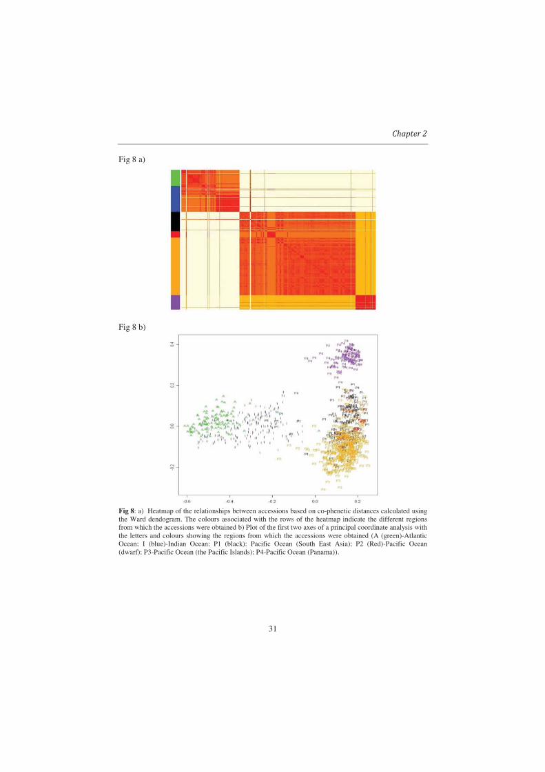
Fig 8 a)

Fig 8 b)

Fig 8: a) Heatmap of the relationships between accessions based on co-phenetic distances calculated using the Ward dendogram. The colours associated with the rows of the heatmap indicate the different regions from which the accessions were obtained b) Plot of the first two axes of a principal coordinate analysis with the letters and colours showing the regions from which the accessions were obtained (A (green)-Atlantic Ocean; I (blue)-Indian Ocean; P1 (black): Pacific Ocean (South East Asia); P2 (Red)-Pacific Ocean (dwarf); P3-Pacific Ocean (the Pacific Islands); P4-Pacific Ocean (Panama)).

32

b) Potato

Data The data used in this study consisted of 233 diploid accessions genotyped

with 50 SSR markers. The accessions were collected from different regions of South America

(Bolivia – 44; Colombia – 80; Ecuador – 16 and Peru - 91). Potato is an out-crossing species

with a substantial level of self-pollination. The 233 diploid accessions came from four species (S.

ajanhuri (22); S. goniocalix (47); S. phureja (105) and S. stenotomum (59)).

Dendrogram, CPCC and AC Dendrograms are given in Fig 9. The potato data

showed many more differences between the results of the different clustering algorithms than the

coconut data. Ward (CPCC = 0.62) performed poorly in preserving the original pair wise

distances between accessions compared to UPGMA (CPCC = 0.89). With regard to quantification

of the hierarchical structure the difference between Ward (AC = 0.94) and UPGMA (AC = 0.77)

was smaller than for the coconut data (0.97 for Ward versus 0.58 for UPGMA).

Fig. 9: Dendrograms for potato for Ward (A) and UPGMA (B). Clear differences can be observed amongst the clustering techniques. Ward dendrogram had Cophenetic Correlation Coefficient (CPCC) of 0.62 and Agglomerative Coefficient (AC) of 0.94 while UPGMA had CPCC of 0.89 and AC of 0.77.

Determining the optimum number of clusters The criteria for determining the number

of clusters applied to the Ward did not agree on the optimum number of clusters (PBC: 4; C-

index: 2; ASC: 6 and FST-based method: 3). C-index had local optima at four and three clusters

(Fig. 10). A similar disagreement was observed with the UPGMA dendrogram (PBC: 3; C-Index,

FST and ASC: 2). It should be noted that the groups resulting from the two dendrograms were of

33

different sizes and compositions. For STRUCTURE, the plot of log-likelihood versus the number

of groups K did not provide a clear indication of the optimum number of clusters. However, for

potato it is clear that the number of clusters is less than eight (there is a sharp drop after k=5).

Fig 10: Plot of the criteria for determining the optimum numbers of clusters for UPGMA and Ward dendrograms for potato data. For PBC (A), ASC (B) and FST-based criteria (D), the number of clusters with the maximum value of the criteria (or the number where the graph starts leveling off) is the optimum; the opposite applies to C-index (C).

Composition of clusters While Ward split accessions into two major clusters S. ajanhuri

(mainly accessions from Bolivia and Peru) versus the other species (S. goniocalix, S. phureja and

S. stenotomum; accessions from Colombia and Ecuador), UPGMA first isolated three accessions

of S. ajanhuri (all from Bolivia) from all other accessions. As for coconut, most clusters formed

by cutting UPGMA trees consisted of 1 or 2 accessions.

In terms of composition of clusters, results of STRUCTURE and Ward showed a good agreement

(see Fig. 11). For example, for K =2 STRUCTURE and Ward both split the accessions into S.

ajanhuri (from Bolivia and Peru) versus S. goniocalix, S. phureja and S. stenotomum (from

Colombia and Ecuador).

34

Fig 11 a) Bar plots for individual potato accessions generated by cutting the Ward dendrogram into 2, 3, 4 or 5 groups (from top to bottom). Groups are represented by different colours. Each column represents one accession. The labels below indicate the potato species.

Fig 11 b) Bar plot for individual potato accessions generated by STRUCTURE 2.2 using the admixture model with independent allele frequencies based on 50 SSR markers for 2, 3, 4 or 5 groups (from top to bottom). Groups are represented by different colours. Each column represents one accession. Bars may consist of different segments representing its composition; the longer a segment the more an accession resembles the corresponding cluster. The labels below indicate the potato species.

35

c) Common Bean (Phaseolus vulgaris)

Data The data consisted of 603 accessions with 296 being described as

Andean and 307 as Mesoamerican types genotyped with 36 SSR markers. These accessions

originated from 24 different countries, most of them coming from Peru (184), Mexico (183),

Guatemala (62), Ecuador (37), Colombia (30) and Brazil (24).

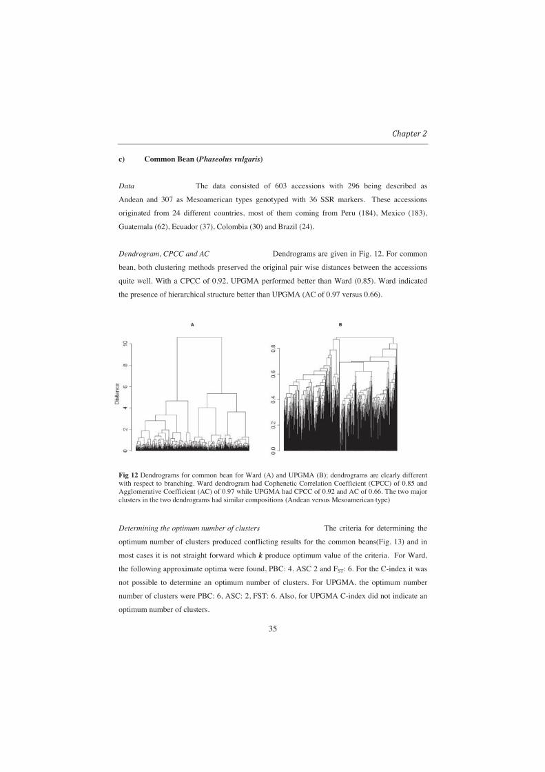
Dendrogram, CPCC and AC Dendrograms are given in Fig. 12. For common

bean, both clustering methods preserved the original pair wise distances between the accessions

quite well. With a CPCC of 0.92, UPGMA performed better than Ward (0.85). Ward indicated

the presence of hierarchical structure better than UPGMA (AC of 0.97 versus 0.66).

Fig 12 Dendrograms for common bean for Ward (A) and UPGMA (B); dendrograms are clearly different with respect to branching. Ward dendrogram had Cophenetic Correlation Coefficient (CPCC) of 0.85 and Agglomerative Coefficient (AC) of 0.97 while UPGMA had CPCC of 0.92 and AC of 0.66. The two major clusters in the two dendrograms had similar compositions (Andean versus Mesoamerican type)

Determining the optimum number of clusters The criteria for determining the

optimum number of clusters produced conflicting results for the common beans(Fig. 13) and in

most cases it is not straight forward which k produce optimum value of the criteria. For Ward,

the following approximate optima were found, PBC: 4, ASC 2 and FST: 6. For the C-index it was

not possible to determine an optimum number of clusters. For UPGMA, the optimum number

number of clusters were PBC: 6, ASC: 2, FST: 6. Also, for UPGMA C-index did not indicate an

optimum number of clusters.

36

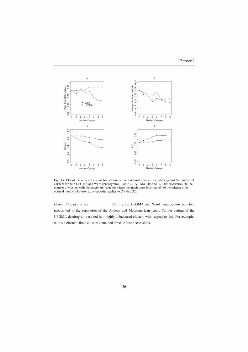
Fig: 13: Plot of the values of criteria for determination of optimal number of clusters against the number of clusters for both UPGMA and Ward dendrograms. For PBC (A), ASC (B) and FST-based criteria (D), the number of clusters with the maximum value (or where the graph starts leveling off) of the criteria is the optimal number of clusters; the opposite applies to C-index (C).

Composition of clusters Cutting the UPGMA and Ward dendrograms into two

groups led to the separation of the Andean and Mesoamerican types. Further cutting of the

UPGMA dendrogram resulted into highly unbalanced clusters with respect to size. For example,

with six clusters, three clusters contained three or fewer accessions.

37

Appendix 2: Additional results from simulated data

Fig. 14 shows a sample of dendrograms for Ward and UPGMA obtained using simulated data

sets. These dendrograms show again that usually Ward dendrograms are highly balanced,

dividing objects in major groups, whereas UPGMA dendrograms are usually highly unbalanced,

forming small groups of objects.

Fig 14: UPGMA and Ward dendrograms for three simulated data sets of different subpopulation differentiations (FST = 0.009 (A), 0.05(B) and 0.1(C)). The dendrograms show changes in CPCC, AC and branching patterns as subgroup differentiation increase from A to C.

Determining the optimum number of clusters From the simulations, it was

only possible to get sensible results when the criteria for determination of optimum number of

clusters were applied to Ward. Cutting of UPGMA dendrograms resulted into highly unbalanced

38

groups. The performance of the criteria for determining the optimum number of clusters rules also

depended on the level of differentiation between subpopulations(see Table 2). The simulation

results indicated that with weak population differentiation (FST <0.08), all methods performed

quite poorly in identifying the correct number of groups. With relatively weak differentiation

between subpopulations, most criteria for determination of optimum number of clusters indicated

two as the appropriate number of clusters. We also noticed that with weak differentiation between

subgroups values of the criteria kept fluctuating to the extent that it was not possible to determine

a knee or a dip indicating an optimal number of clusters. Beyond a certain level of population

differentiation (FST > 0.2) the performance of all criteria become quite similar (see Table 2).

Table 2 Percentage of simulated data sets (based on 30 datasets per group) in each category for which each criteria for determining the number of clusters identified the correct number of clusters (results from Ward only) Criteria

Group mean FST ASC (%) PBC (%) C-index (%)* FST (%)**

0.0123 0 0 3.3 20 0.0347 23 43 27 20 0.0637 73 80 50 77 0.0836 87 90 53 97 0.1335 93 93 67 100 0.1998 93 93 77 100 0.2503 100 93 100 100 0.3039 100 100 100 100 0.3528 100 100 100 100

*C-Index: This criterion is only based on distances between objects within clusters and is calculated as

follows: )/()( minmaxmin SSSSIndexC =in which S is the sum of pair wise distances between objects within the same cluster summed over all

clusters. If l is the number of pairs of objects used to calculate S, then minS and maxS are the sum of the l

smallest and the l largest distances between all pairs of objects (i.e. ignoring the presence of clusters). **FST-based criterion: FST directly measures genetic divergence among clusters. Wright (1951; 1965) defined FST as the correlation between two alleles chosen at random within a subpopulation relative to alleles sampled at random from the total population. In this case, FST is calculated between clusters obtained by cutting dendrograms into specified numbers of clusters. Theoretically, the optimum number of clusters should result in the highest FST-value. In this paper the analysis of variance (ANOVA) approach was used to calculate FST, more specifically the algorithm of Yang (1998) as implemented in the Hierfstat package of R (Goudet 2005).

T.L. Odong • J. van Heerwaarden • J. Jansen • Th.J.L. van Hintum • F.A. van Eeuwijk Principal components analysis improves ability of hierarchical cluster analysis methods for recovering the genetic structure of germplasm collections

Chapter 3

Principal components analysis improves ability of hierarchical cluster analysis

methods for recovering the genetic structure of germplasm collections

Abstract

Understanding the genetic structure of germplasm collections is a prerequisite for effective and

efficient utilization of genetic resources stored in genebanks. Although recent developments in

genetics and statistics have led to the development of new tools for studying genetic structure of

populations, the old, and usually simpler approaches such as hierarchical cluster analysis are still

very popular with scientists. Our study explores the potential of combining two classical

multivariate statistical techniques, cluster analysis and principal component analysis (PCA), for

understanding the genetic structure of germplasm collections. The two-step approach involves

first applying PCA to molecular marker data followed by cluster analysis using significant

principal components (PC) only. The determination of the number of significant PC is done

using the Tracy-Widom (TW) distribution. The parameters of the TW distribution only depend

on the dimensions of the allele frequency matrix. In this study we compared the performance of

cluster analysis (Ward and model-based hierarchical clustering) using reduced sets of significant

PC with cluster analysis using the full data set. For reduced sets of PC, Ward’s clustering was

performed on Euclidean distances, while for the full data sets three other distance measures

(proportion of shared alleles, Jaccard and simple matching) were used. Clustering (Ward and

model-based clustering) using reduced sets of PC performed much better than clustering using

full data sets both in terms of recovering groups as well as in determining the exact number of

groups. The improvement in performance was most noticeable in cases with low population

structure. In conclusion, PCA in combination with cluster analysis provides a very useful tool for

studying genetic structure of heterogeneous germplasm collections, which can be carried out

using standard statistical software.

40

3.1 Introduction

Knowledge of the genetic structure of heterogeneous germplasm collections is essential

when forming core collections (Brown 1995; van Hintum et al. 2000), and in association

studies (Wang et al. 2005; Shriner et al. 2007). Hierarchical clustering techniques such as

Ward and UPGMA are still among the most-used methods for determining structure, and

a recent study by Odong et al. (2011) indicates that they are also very useful when

molecular markers have been used to characterise the collection. Unlike programs such

as STRUCTURE (Pritchard et al. 2001), hierarchical clustering techniques require little

computer time, and moreover, they are simple to use. However, both traditional

clustering algorithms and programs such as STRUCTURE do not always perform very

well with germplasm data especially when it comes to the determination of the number of

clusters. Principal component analysis (PCA) has been suggested to enhance the

performance of clustering techniques (Patterson et al. 2006, Lee et al. 2009). In this

study, we explore the possibility of boosting the performance of hierarchical cluster

analysis using PCA.

Recent developments in population genetics theory have provided interesting avenues for

exploiting the information that molecular markers contain about population

differentiation. It has been shown that there is a direct theoretical relationship between

population genetic structure and principal components (Patterson et al. 2006, McVean,

2009). In particular, the distribution of eigenvalues associated with principal components

is determined by the number of independent sources of differentiation (i.e.

subpopulations) present in the dataset. Moreover, the distance between groups along the

major PCs has been shown to be proportional to the level of genetic differentiation

(McVean, 2009). PCA has been successfully used with SNP data for determining the

number of different populations (Patterson et al. 2006) and to assign individuals to these

populations (Lee et al. 2009). The usefulness of this novel application of PCA in

understanding the genetic structure of germplasm collections is yet to be exploited,

especially using multi-allelic markers such as Single Sequence Repeat (SSR) markers.

SSR markers are still among the most commonly used molecular markers for germplasm

41

characterization. For PCA to be useful for determining the number of subpopulations, the

assumptions are a) the number of markers is greater than the number of individuals and b)

the molecular markers used should be independent or unlinked (Patterson et al. 2006). It

should be noted that unlike the SNP data used in previous studies (Patterson et al. 2006;

Lee et al. 2009 ) in which the markers are usually much greater in number than the

individuals, in most germplasm collection data, this difference (between number of

individuals and number of markers) is much smaller. In addition, when SSR markers are

treated as binary markers (each allele is coded 0 (absent) or 1 (present)), the assumptions

of independence of the different columns in the data matrix is violated.

Because of the multi-allelic nature of SSR markers, various methods for determining the

(dis)similarity (hereafter referred to as distances) between individuals or subgroups exist;

there is no standard way of handling SSR markers. For example, when SSR markers are

treated as binary markers (each allele is coded for presence or absence), a binary-based

distance measure such as Jaccard (Jaccard 1908) can be applied (Anthony et al. 2002;

Cordeiro et al. 2003; Balestre et al. 2008). Another common distance measure for SSR

markers is based on the proportion of shared alleles (Chakraborty and Jin 1994; Chang et

al. 2009). The performance of different distance measures for cluster analysis has not yet

been extensively evaluated. In this study, we use real and simulated data sets to explore

the effect of data reduction using PCA on the clustering of germplasm collections using a

traditional hierarchical clustering technique (Ward’s method) and a model-based

hierarchical clustering technique (Mclust, mixture of normal distributions; Fraley and

Raftery 2002; Fraley 2006). Ward and UPGMA are the two most commonly used

hierarchical clustering techniques in plant germplasm studies. Ward was selected for this

study because it has been shown to perform much better with molecular marker data than

UPGMA (Odong et al. 2011). Model-based clustering was used previously with SNP

data and shown to perform quite well (Lee et al. 2009). We also evaluated the effect of

different distances measures (Euclidean, proportion of shared alleles (Bowcock et al.

1994, Chang et al. 2009), Jaccard (Jaccard 1908) and simple matching (Sokal and

Michener 1958) for clustering germplasm collections using SSR markers.

42

3.2 Materials and Methods

3.2.1 Description of data sets

Real data

A coconut (Cocos nucifera) data consist of 1014 accessions genotyped with 30 SSR

markers. The accessions were collected from different regions of the world (West Africa

– 32; North America – 52; South Asia – 62; Latin America – 72; Central America & the

Caribbean – 109; East Africa – 124; South East Asia – 183; the Pacific Islands - 380).

Coconut is a diploid, mainly out-crossing species. Most of the accessions in this

collection are described as tall; only 43 dwarf accessions mainly from South East Asia

were present. Dwarf coconuts have a high degree of self-fertilization. More than half (19)

of the 30 SSR markers have known positions on the linkage map; they are well spread

across the genome.

Simulated data

Marker data were simulated using SimuPOP (Peng and Kimmel 2005), a forward-time

population genetic simulation environment. We used a finite island model (Wright 1931)

and a stepping stone (Kimura 1953) migration model. In each generation, random mating

(with 2% selfing) was assumed to produce diploid genotypes for 30 unlinked loci. We

simulated 1000 individuals in five and eight subpopulations and 750 individuals in 15

subpopulation with varying levels of subpopulation differentiation (differentiation

between subpopulations is determined by migration rate and number of generations). The

migration rates used in this study were 0, 1 and 2 migrants per subpopulation per

generation . At each of the 30 loci, the average allele frequencies of the coconut data

were used as the starting allele frequencies for the simulation. Within each parameter set,

all loci had the same mutation dynamics, according to a K-allele model (KAM). Under

the KAM model, there are K possible allelic states, and any allele has a constant

probability of mutating into any of the other K–1 allelic states (Crow and Kimura 1970).

A mutation rate of 2 x 10-5 with 50 possible allelic states was used in the simulation.

The mutation parameters were set to mimic highly polymorphic markers such as SSR

43

markers. However, in this case the role of mutation is very limited since we used a

limited number of generations in the simulation. In addition to using alleles from real

data as starting frequencies for simulation, the numbers of generations for the simulations

were restricted (from 5 to 200 generations) to mimic the situation of agricultural crops in

genebanks.

3.2.1 Genetic distance measures

Because SSR markers are multi-allelic in nature genetic similarities or dissimilarities

(hereafter referred to as distances) between individuals or groups are calculated in several

ways. In this paper, four different types of genetic distances between accessions were

used.

a) Distance based on proportion of shared alleles

The genetic distance (D) between individuals (accessions) i and j based on the proportion

of shared alleles (PSA) was calculated as

D_PSA ij = 1 – PSAij,

Where LffPSA jla

L

l

A

ailaij

l

/),min(1 1= =

= .

In diploids ilaf and jlaf represent the frequencies of allele a ( a =1, 2… lA ; lA is the total

number of alleles for molecular marker l ( l =1, 2… L ) in individuals i and j, respectively;

i j = 1, 2 … N). It should be noted that in this paper PSAij refers to proportion of shared

alleles between (diploid) individuals rather than populations; as a consequence

1or,0, 21=jlaila ff . For more information on the proportion of shared alleles as

similarity measure between populations, see Bowcock et al. (1994), Chakraborty and Jin

(1994) and Chang et al. (2009).

44

b) Euclidean distance

The Euclidean or straight line distance between two individuals i and j , having

observations on P quantitative variables denoted as iPii xxx ,...,, 21 and jPjj xxx ,...,, 21 is

given by

2222

211 )(...)()(_ jpiPjijiij xxxxxxEuclD +++= .

In this study the variables Pxxx ,...,, 21 are the principal components obtained from the

molecular marker data.

c) Distances based on coding SSR markers as binary data

For the calculation of genetic distances between individuals, it is common practice to

treat SSR markers as binary markers (Anthony et al. 2002; Cordeiro et al. 2003; Balestre

et al. 2008). In this case, each allele is treated as a binary variable (0 = absence,

1=presence). Because they are among the most frequently used distances in the genetic

diversity studies, the Jaccard (Jaccard 1908) and simple matching (Sokal and Michener

1958) distances have been selected for this study. The major difference between the two

distances is that for Jaccard double-absent matches are ignored, while for simple

matching they are included. It should be noted that the double-absent matches do not

contain useful information in the case of multi-allelic SSR markers. However, simple

matching distance is included in this study for reference purposes. For each allele, the

results of individuals i and j can be summarized in a contingency table:

Individual i

In

divi

dual

j

Present Absent

Present aij bij

Absent cij dij

45

where aij + bij + cij + dij = A (A is total number of alleles for all the L SSR markers).

The distances based on binary coding of SSR markers are calculated as follows

i) Jaccard distance

ijijij

ijij cba

aJACD

++= 1_

ii) Simple matching distance

ijijijij

ijijij dcba

daSMD

+++

+= 1_

It is common to convert similarity measures into distances without using the square root,

but the square root gives distances the Euclidean property (Gower and Legendre, 1986).

The Euclidean property is important, because it is a requirement of many multivariate

analysis methods such as principal coordinate analysis, hierarchical cluster analysis,

hierarchical classification, and graph theory (Gower, 1985). However, empirically we

found that conversion of similarity measures into distance measures with or without using

the square root had no effect on the formation of clusters.

3.2.3 Principal component analysis

PCA does not attempt to classify individuals into discrete subgroups but instead it

characterizes each individual by coordinates (PC) along the major axes of variation. In

this paper we investigate how these coordinates can be used to improve the results of both

hierarchical and model-based clustering methods.

We treat each allele from an SSR marker l as a bi-allelic marker. The data can be

represented as a rectangular matrix G of which the number of rows is equal to number of

individual accessions N and the number of columns is equal to the total number of alleles

(A) (=

=L

llAA

1

, where lA is the number of alleles from SSR marker l (l= 1, 2 …, L )).

46

The matrix G contains allele counts 0, 1 or 2. Before performing PCA, the matrix G is

standardized by subtracting column means followed by dividing columns by their

standard deviation (see Patterson et al. 2006). We performed PCA using the function

prcomp in R.

Determination of eigenvalues and the Tracy Widom test

Eigenvalues

It has been shown recently that, in the absence of genetic structure and for independent

markers, the leading eigenvalue of the covariance matrix of a normalized G matrix

follows a Tracy-Widom (TW) distribution (Tracy 1994; Patterson et al. 2006). This fact

has been exploited to determine the number of genetically different groups in genotypic

datasets (Patterson et al. 2006). If there are k genetically different groups in a dataset, the

number of significant eigenvalues based on TW distribution is expected to be k-1

(Patterson et al. 2006). In performing the TW test, Patterson et al. (2006) assumed that

the SNP being analyzed were independent. It is clear that this assumption will be

violated when the TW test is applied to SSR data since alleles from the same SSR marker

are not independent. To get around this problem, we have adapted the procedure to

handle SSR markers as follows:

a) Perform PCA on a matrix Gl (l =1,2,...L, L is the number of SSR), the sub-matrix of

matrix G containing only alleles from SSR marker l. Let Gl* (l=1, 2, ….., L) be the

matrix of which the columns consist of PC (from matrix Gl) explaining more than

0.5% of the variance. Removing PC which explain less than 0.5% of the variance

eliminates noise so that it will become easier to detect the correct number of major

groups. Removing non-important PC is similar to the idea of determination of the

effective number of alleles.

b) Form a matrix G* of which the columns consist of the columns of the matrices

G1*, G2*,..., GL* obtained from step (a) above. The columns of the matrix G* are

thus effectively independent (when the loci (SSR markers) are independent)

47

leading to an approximate TW distribution of eigenvalues (Tracy, 1994). The

assumptions that markers are independent still holds.

c) Perform an eigenvalue decomposition on the matrix X =n

1 where

G** is obtained by standardizing the matrix G* (from each column of matrix

G*, we subtract the column mean and divide by its standard deviation) and n is

the number of columns of matrix G* .

Tracy-Widom distribution

Patterson et al. (2006) provided a detailed description of the TW distribution and its

application for the detection of population structure. A brief review is provided below.

Following the notation of Patterson et al. (2006), consider an m × n matrix M with

( nm < ),of which each entry contains an independent standard normal random variable.

Let '1MMX

n= , and let { } mkk <<1 be the eigenvalues of X. For ordered eignenvalues

( m>> ...21 ) Johnstone (2001) showed that for a suitably normalized matrix M, and

for large m and n the largest eigenvalue 1 approximately follows a TW distribution

(Tracy and Widom, 1994) with mean ),( nm and standard deviation ),( nm in which

n

mnnm

2)1(),(

+=

3/11

1

1)1(),( +

+=

mnn

mnnm

i.e. the statistic (),(

),(1

nm

nmz = ) follows approximately a standard TW distribution.

Patterson et al. (2006) state, that if the first k eigenvalues have been declared significant,

48

the test for mkk >> ++ ...21 can be carried out as X having dimension )( km x

)( km , and changing mean and variance of the TW distribution accordingly.

When analysing data from germplasm collections, the number of markers (n) is usually

less than the number of individuals ( nm > ) so based on Johnstone (2001), we suggest

that the above formulae must be adapted before performing the TW test (i.e. m =

min(nrow(M), ncol(M)) and n = max(nrow(M), ncol(M)) where nrow(M) and ncol(M)

are the number of rows and columns of the matrix M respectively).

Additional methods for determination of the number of groups

In addition to the TW test we also used two other criteria frequently used for determining

the number of clusters in hierarchical cluster analysis: the point biserial correlation (PBC)

and the average silhouette coefficient (ASC).

PBC (Milligan 1981) is defined as the correlation between the original distance matrix

and a matrix consisting of zeros and ones indicating whether two objects are in the same

cluster or not. This is an easy measure of the resemblance between the distance matrix

(observed relationships) and the resulting tree (fitted relationships).

ASC (Rousseeuw 1987) combines the concepts of cluster cohesion and separation; it

relates distances between objects within the same cluster with distances between objects

in different clusters. The silhouette coefficient ( is ) of an object i is calculated as:

),(max)/( b(i))w(i)b(i))w(i) ddddsi = , where w(i)d is the average distance of an object i to

all the individuals in the same cluster and )(ibd is the minimum of the average distance

between an object i and objects in another single cluster (i.e. for every cluster to which

object i does not belong, the average distance between an object i and objects in that

cluster is calculated (separately), and the minimum of those averages is )(ibd ). The

average silhouette coefficient for a cluster is calculated by averaging the silhouette

coefficients of all the objects in the cluster. The overall measure of the quality of the

clustering (ASC) is obtained by computing the average silhouette coefficients over of all

objects in the data.

49

3.2.4 Cluster analysis results

We explored the potential of using significant PC (expected to be the first k-1 PC in a

situation with k subpopulations) to improve the performance of hierarchical clustering.

Ward’s clustering algorithm (Ward, 1963; Johnson and Wichern, 2002) was selected for

this study because it is one of the most used clustering methods and has been shown to

perform relatively well (see Odong et al 2011). Ward’s method employs an analysis of

variance (ANOVA) approach for calculating distances between clusters. For each pair of

clusters, at each step in the clustering process, the effect of the union of every possible

pair of clusters is considered, and the two clusters that produce the smallest increase in

within group sum of squares are joined. Ward’s method was used with a) Euclidean

distances based on different numbers of PC b) distances based on the proportion of

shared alleles c) distances based on SSR markers coded as binary markers (Jaccard and

Simple matching).

The performance of cluster analysis using Ward’s method was compared with that of

model-based Gaussian hierarchical clustering (Fraley, 1998) using significant PCs. This

method assigns individuals to groups by fitting a mixture of multivariate normal

distributions to the data. The estimation of model parameters and assignment of

accessions to groups is done by the Expectation Maximization (EM) algorithm (Banfield

and Raftery, (1993)). In this case the geometric features (shape, volume and orientation)

of the clusters are determined by the covariance structures. We used the implementation

provided by the R package mclust (Fraley and Raftery, 2006). Several covariance models

were tested and the spherical variable volume was found to fit our data best, and this

model was used for all subsequent analyses. In this model, all clusters are assumed to

have a spherical shape with different volumes depending on the variance within each

cluster (see review by Fraley and Raftery, 2002).

50

Evaluating the performance of cluster analysis based on different genetic distances

In this study, the success of cluster analysis was measured using i) cluster purity and ii)

the adjusted rand index (see below). The adjusted rand index was also used to compare

the similarity of groups formed by clustering using different distance measures. To

explore the effect of the number of PCs used in cluster analysis, we looked at the

correlation between the group membership matrix and Euclidean distances between

accessions based on the first n PC (only for simulated data). The performances of the two

criteria for evaluation of the number of clusters were compared with testing for the

number of subgroups using the TW distribution.

Cluster purity

For the simulated data, the ability of clustering techniques to recover the subpopulations

was evaluated using overall cluster purity (Zhao and Karypis 2004). Overall cluster purity

is calculated as follows. Let r

rqrq w

wp = be the probability that an accession is allocated to

cluster r (r = 1,2, …, R) belongs in reality to subpopulation q (q = 1, 2,…., Q), rqw is

the number of members of subpopulation q allocated to cluster r and rw is the number

of objects in cluster r . The purity for each cluster ( rp ) is defined as the maximum

probability of correct assignment of objects in cluster r to one of the subpopulations, i.e.

( ),max rqq

r pp = and over all purity is defined as =

R

rr

r pw

w

1

. For the coconut data, the

groups formed by clustering using different genetic distances were related to their

passport data (country of origin).

Adjusted rand index

The adjusted rand index (Hubert and Arabie, 1985) assesses the degree of agreement

between two partitions of the same objects. In this study the adjusted rand index was

used to compare the grouping based on cluster analysis to known groups (obtained

51

through simulation). We also used the adjusted rand index to study the similarities

between groups formed using Ward’s method with different genetic distance measures.

A brief description of adjusted rand index is given below (detailed mathematical

description see Santos and Embrechts, 2009).

Consider a set of N objects (or individuals) { }NOOOS ,...,, 21= (Oi = object i; i =1,

2,...,N) and suppose that },...,,{ 21 RuuuU = and { }QvvvV ,...,, 21= represent two different

partitions (e.g. cluster analysis groupings versus true simulated subpopulations) of the

individuals in S such that qQqr

Rr vSu 11 == == and qqrr vvuu == for

Rrr'1 and Qqq1 . Given two different partitions U and V, with R and Q

subsets, respectively, the contingency table can be formed to indicate group overlap

between U and V (see Table 1).

Table 1: Contingency table for comparing partitions U and VPartition* V Group

1v 2v ...Qv Total

1u 11t 12t ...Qt1 .1t

U 2u 21t 22t ...

Qt2 .2t.. .

.

.

... .

.

.

... .

.

.

.

Ru 1Rt 2Rt ...RQt .Rt

Total 1.t 2.t ...

Qt. Nt =..

* trq, represents the number of individuals that were classified in the rth subset of partition U and in the qth subset of partition V.

The total number of possible combinations of pairs 2

N from a given set of individuals

can be divided into in four different types of pairs:

2/1 1

21 =

= =

R

r

Q

qrq Ntg - number of pairs of individuals placed in the same group by

using methods U and V (e.g. using cluster analysis and according to the groups used for

simulating the marker data );

52

2/1 1 1

22.2 =

= = =

R

r

R

r

Q

qrqr ttg - number of pairs of individuals put in same group by method

U and different groups by methods V;

2/1 1 1

22.3 =

= = =

Q

q

R

r

Q

qrqq ttg -number of pairs of individuals that are put in the same group

by method V but in different groups by method U and, finally,

3214 2ggg

Ng = - number of pairs of individuals that are put in different groups

by both methods U and V.

The rand index R_index is given by

+=

2

_ 21

N

ggindexR ,

Hubert and Arabie (1985) introduced the correction for chance so that the expected value

of the rand index is zero for random partitions.

The adjusted rand index (AR_index) is given by

)])(())([(2

)])(())([()(2

)_()_(

)_(__

42433121

2

4243312141

ggggggggN

ggggggggggN

indexREindexRMax

indexREindexRindexAR

+++++

++++++

==

,

where )_( indexRE represents the expected value of R_index and )_( indexRMax the

maximum value of R_index (see Hubert and Arabie, 1985 for details); AR_index has

expectation zero and maximum 1.

Correlation between the group membership matrix and genetic distances

This correlation is used to determine the effect of the number of PC (used for calculating

distances) on the distortion of relationship between individuals both within and between

groups. Elements of the group membership matrix are either one (if two accessions

53

belong to the same population) or zero (if two accessions belong to different

populations). This correlation was only used for the simulated data when group

membership is known exactly .

3.3 Results:

3.3.1 Coconut data

A PCA of the coconut data reveals the presence of significant population structure. The

total number of significant PC is 14, explaining 21.3 percent of variance. The correlation

between Euclidean distances based on the first 14 PC with other genetic distances ranged

from 0.512 (with simple matching) to 0.700 (with proportion of shared alleles).

Distances based on SSR coded as binary markers (Jaccard and simple matching) are

highly correlated (0.884) among themselves but also with distances based on the

proportion of shared alleles (0.869 and 0.919 with simple matching and Jaccard,

respectively).

Clustering using Ward’s method and model-based clustering using the first 14 PC

resulted into 15 groups which coincided well with the region of origin of the accessions

(see Table 2). The large group of Pacific accessions (PCF) were clustered into seven

groups (six for model-based clustering), whereas accessions from Central America (CA)

and South East Asia were each clustered into two groups. Accessions from West Africa

(WA), Latin America (LA), South Asia and East Africa each formed one group, with

both Ward’s method and model-based clustering. The South East Asian Dwarf accessions

(SEA2) also formed a single cluster with Ward’s method but two with model-based

clustering. Analysis of the seven groups of accessions from the Pacific formed by Ward

(using Euclidean distance) showed good associations with specific islands or groups of

islands. For example, the largest group (135) has 80% of the accessions coming from

Papua New Guinea; accessions from the South Pacific (Fiji, Cook Island, Tonga and

French Polynesia) form one group, accessions from the Mid Pacific (Marshall Islands,

Kirivatu and Tuvalu) form their own group too (see Appendix 1).

54

Groups formed with Ward’s method using other distance measures (proportion of shared

alleles, Jaccard and simple matching) differ from groups formed with Ward’s method

using Euclidean distances (based on the 1st 14 PC) in the grouping of accessions from

the Pacific, South Asia and South East Asia. It can be seen from Table 2 that accessions

from South Asia and South East Asia form more than one group when clustering is done

using Ward’s method with distances based on proportion of shared alleles. For the

accessions from the Pacific Islands the correspondence between the islands as origins of

accessions and the groups formed by Ward’s method with distances based on the

proportion of shared alleles distances is poor (see Appendix 1). For example, accessions

from Papua New Guinea and Vanuatu no longer form their own separate groups when

clustering is done using Ward’s method with distances based on the proportion of shared

alleles.

The level of agreement between groups formed by Ward’s method using different

distance measures depends on the number of groups the accessions are clustered into.

When the dendrogram is cut into two or three groups (major groups in the data), all

values of the adjusted rand index are above 0.96. However, when dendrogram is cut into

fifteen clusters (number of clusters predicted by the TW test), the agreements between the

groups formed using different distances are considerably smaller (values range from

0.468 to 0.771) (see Table 3).

55

Table 2: The distribution of accessions from different origins into the 15 clusters formed

using Ward’s method with Euclidean distance (14 PCs) and, distance based on proportion

of shared alleles and model-based clustering . Cluster numbering is arbitrary

Euclidean distances based on 1st 14 PCs (E-r) Origin1 1 2 3 4 5 6 7 8 9 10 11 12 13 14 15 CA 80 23 - - - - - - - - - - 2 - - CAR - - - - - - - - - - - 2 - - 2 EA - - 115 - - - - - - - - 9 - - - LA - - - 69 - - - - - - - - 1 - 2 NAM1 - - - - 2 3 9 - - - - - 29 - - NAM2 - - 1 - - - - - - - - 8 - - - PFC - - - - 135 18 114 27 15 20 41 - 3 3 - PFC2 - - - - 2 - - - - - - - - 2 - SA - - 7 1 1 - - - - - - 41 - 3 9 SEA - - 1 - 13 5 - - - - - 5 115 4 - SEA2 - - - - - - - - - - - - 5 35 - WA - - - - - - - - - - - - - 3 29

Model-based clustering using 1st 14 PCs (MC) Origin 1 2 3 4 5 6 7 8 9 10 11 12 13 14 15 CA 79 23 1 - - - - - - - - - 1 1 - CAR - - - - - - - - - - 3 - - - 1 EA - - 116 - - - - - - - 8 - - - - LA - - 6 63 - - - - - - 3 - - - - NAM1 - - - - - 1 9 1 - - - - 31 1 - NAM2 - - - - - - - - - - 9 - - - - PFC - - - - 111 65 115 14 25 36 - 3 5 2 - PFC2 - - - - 1 - - - - - - 2 - 1 - SA - - 7 2 - - - - - - 49 1 - 2 1 SEA2 - - - - - - - - - - - 22 1 17 - SEA - - 3 - 5 7 2 - - - 5 1 104 16 - WA - - - 2 - - - - - - 6 - - 3 21

Distances based proportion of shared alleles (PS) Origin 1 2 3 4 5 6 7 8 9 10 11 12 13 14 15 CA 102 1 - - - - - - - - - 1 - 1 - CAR - - 1 - - - - - - - - - - - 3 EA - 116 - - - - - - - 2 6 - - - - LA - 5 66 - - - - - - - 1 - - - - NAM1 - - - 1 - 7 - - - 6 - 1 - 28 - NAM2 - - - - - - - - - - 9 - - - - PFC - 1 - 85 78 69 24 14 32 61 - 7 3 2 - PFC2 - - - - - - - - - 2 - - 2 - - SA - 12 - - - - - - - - 30 - 3 - 17 SEA - 6 - 1 3 3 - - - 27 - 54 10 39 - SEA2 - - - - - - - - - - - 1 39 - - WA - - - - - - - - - - - - 3 - 29 1CA: Central America (Panama), CAR: Caribbean, EA: East Africa, LA: South America (Brazil), NAM1: North America (Pacific), NAM2: North America (Atlantic), PFC: Pacific Islands, PFC2: Pacific Islands (dwarf), SEA: South East Asia, SEA2: South East Asia (dwarf), WA: West Africa

56

Table 3: Adjusted rand index showing the agreement between groups formed by Ward’s method using different genetic distances. The groups are formed by cutting the dendrogram into 2, 3, 4 and 15 clusters. The agreement between groups formed by different distance measures reduces when the number of clusters increases Two clusters Three clusters

E-r1 1.000 1.000

PS 0.968 1.000 0.974 1.000

Jaccard 0.984 0.976 1.000 0.983 0.979 1.000

SM 0.980 0.972 0.980 1.000 0.984 0.975 0.982 1.000

Four clusters Fifteen clusters

E-r 1.000 1.000

PS 0.693 1.000 0.468 1.000

Jaccard 0.704 0.965 1.000 0.456 0.500 1.000

SM 0.880 0.687 0.693 1 0.545 0.578 0.573 1.000

E-r PS Jaccard SM E-r PS Jaccard SM 1E-r - Euclidean distance based on the first k-1 PCs, PSA: distance based on proportion of shared alleles, SM: simple matching distance

3.3.2 Simulated data

Relationship between different genetic distances

Euclidean distances based on the first k-1 PC (k is the number of subpopulations in the data)

have a low to moderate correlation with the other genetic distances (proportion of shared

alleles, Jaccard and simple matching). This correlation increases with the strength of subgroup

differentiation (see Fig 1). The distances based on SSR markers coded as binary markers

(Jaccard and simple matching) are highly correlated (on average 0.917) among themselves

and this correlation is less affected by the strength of subgroup differentiation. Distances

based on proportion of shared alleles also have a high correlation with distances based on SSR

coded as binary markers (on average 0.876 and 0.845 with Jaccard and simple matching,

respectively).

57

Fig 1: A plot of the correlations between Euclidean distances based on the first k-1 PC (k is the number of subpopulations in the data) and other genetic distances (PSA: distances based on the proportion of shared alleles, SM: simple matching distance) against the population differentiation (FST) for a data set with five (k = 5) subgroups.

Clustering success (Cluster purity and Adjusted Rand Index)

The ability of Ward’s method to recover the original groups in the data (based on cluster

purity and adjusted rand index) increases with the number of PC used for calculating

distances between accessions before levelling off at the first k-1 PC (see Fig 2). For data sets

with the highest number (15) of subgroups, the levelling off takes place at a number of PC

less than k-1 when subgroup differentiation is high. The increase in cluster purity and

adjusted rand index was also observed for model-based clustering (result not shown).

However for model-based clustering, as the number of PCs increases beyond k-1 the results

(cluster purity and adjusted rand index) become more erratic.

58

Fig 2: Plot of cluster purity verses the number of PC used for performing cluster analysis using Ward’s method for simulated data with different number of subgroups (5, 8 and 15) and different levels of genetic differentiation (FST).

Clustering with Ward’s method using Euclidean distances calculated using the first k-1 PC

performs much better than clustering using other genetic distances especially at low levels of

subgroup differentiation. Results of Ward’s method using the first k-1 PC are similar to those

of model-based clustering for all levels of subgroup differentiation. Euclidean distances

based on all PC produced the worst results (see Fig 3).

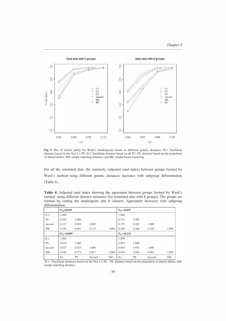
59

Fig 3: Plot of cluster purity for Ward’s dendrograms based on different genetic distances (E-r: Euclidean distance based on the first k-1 PC; E-f: Euclidean distance based on all PC; PS: distance based on the proportion of shared alleles; SM: simple matching distance) and MC: model-based clustering

For all the simulated data, the similarity (adjusted rand index) between groups formed by

Ward’s method using different genetic distances increases with subgroup differentiation

(Table 4).

Table 4: Adjusted rand index showing the agreement between groups formed by Ward’s method using different distance measures (for simulated data with 8 groups). The groups are formed by cutting the dendrogram into 8 clusters. Agreement increases with subgroup differentiation

FST=0.025 FST =0.037

E-r1 1.000 1.000

PS 0.106 1.000 0.323 1.000

Jaccard 0.113 0.093 1.000 0.375 0.265 1.000

SM 0.109 0.091 0.132 1.000 0.369 0.264 0.356 1.000

FST =0.069 FST =0.121

E-r 1.000 1.000

PS 0.810 1.000 0.957 1.000

Jaccard 0.827 0.763 1.000 0.963 0.953 1.000

SM 0.838 0.772 0.817 1.000 0.963 0.956 0.963 1.000

E-r PS Jaccard SM E-r PS Jaccard SM 1E-r – Euclidean distances based on the first k-1 PC, PS: distance based on the proportion of shared alleles, SM: simple matching distance

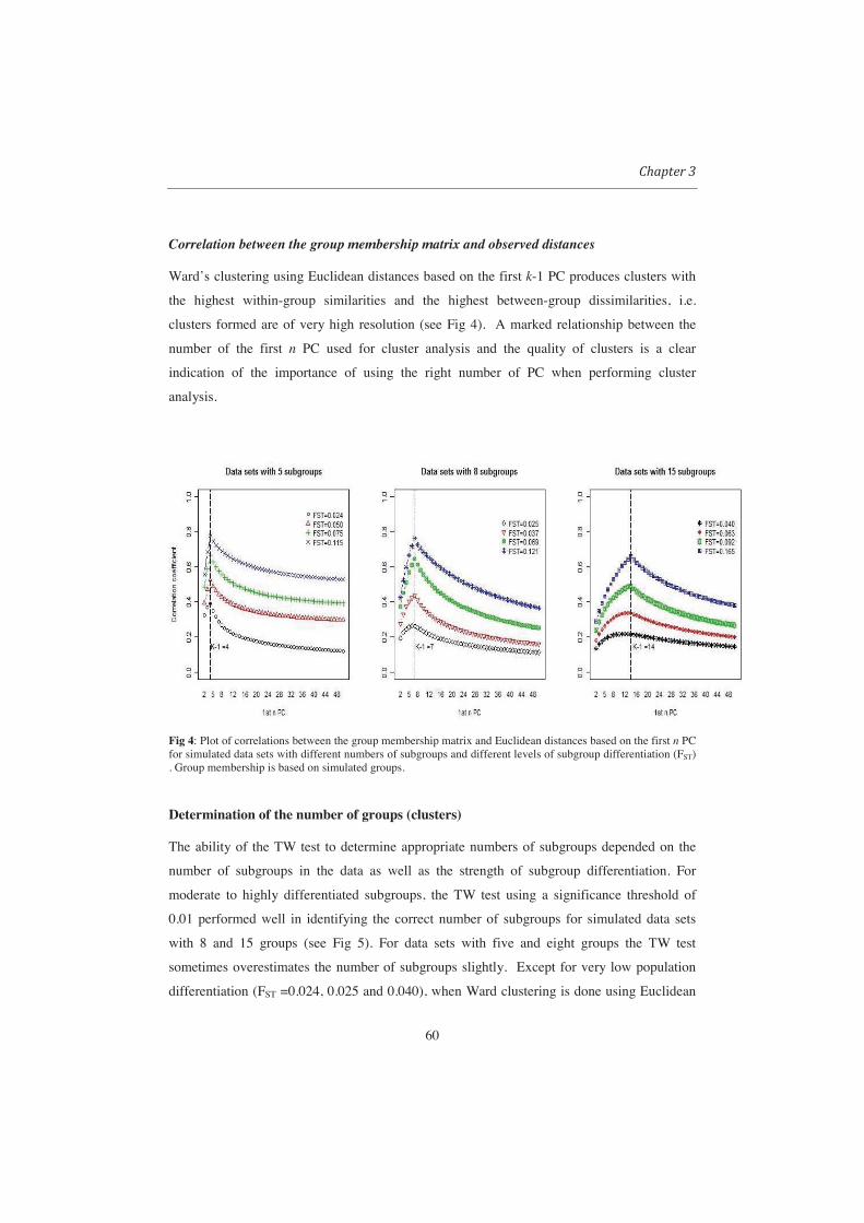
60

Correlation between the group membership matrix and observed distances

Ward’s clustering using Euclidean distances based on the first k-1 PC produces clusters with

the highest within-group similarities and the highest between-group dissimilarities, i.e.

clusters formed are of very high resolution (see Fig 4). A marked relationship between the

number of the first n PC used for cluster analysis and the quality of clusters is a clear

indication of the importance of using the right number of PC when performing cluster

analysis.

Fig 4: Plot of correlations between the group membership matrix and Euclidean distances based on the first n PC for simulated data sets with different numbers of subgroups and different levels of subgroup differentiation (FST) . Group membership is based on simulated groups.

Determination of the number of groups (clusters)

The ability of the TW test to determine appropriate numbers of subgroups depended on the

number of subgroups in the data as well as the strength of subgroup differentiation. For

moderate to highly differentiated subgroups, the TW test using a significance threshold of

0.01 performed well in identifying the correct number of subgroups for simulated data sets

with 8 and 15 groups (see Fig 5). For data sets with five and eight groups the TW test

sometimes overestimates the number of subgroups slightly. Except for very low population

differentiation (FST =0.024, 0.025 and 0.040), when Ward clustering is done using Euclidean

61

distance based on significant PC (even when TW test failed to predict the true number of

subgroups), ASC and PBC always identified the correct number of groups (see Fig 6). When

model-based clustering was done using significant PCs, the clustering process converge on

the right number of clusters except for data sets with low subgroup differentiation (result not

shown).

Fig 5: Distributions of the number of groups determined using Tracy-Widom distribution (test) for data sets with different numbers of groups (5, 8 and 15) and different levels of population structure (FST). Box plots are based on 20 data sets with similar FST values .

When other distance measures (proportion of shared alleles, Jaccard and Simple matching)

were used in combination with Ward’s clustering there were no differences in the

performance of the two criteria (ASC and PBC) for determining the number of clusters.

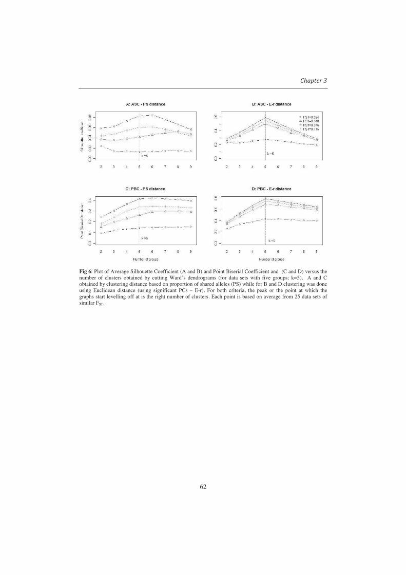
62

Fig 6: Plot of Average Silhouette Coefficient (A and B) and Point Biserial Coefficient and (C and D) versus the number of clusters obtained by cutting Ward’s dendrograms (for data sets with five groups; k=5). A and C obtained by clustering distance based on proportion of shared alleles (PS) while for B and D clustering was done using Euclidean distance (using significant PCs – E-r). For both criteria, the peak or the point at which the graphs start levelling off at is the right number of clusters. Each point is based on average from 25 data sets of similar FST.

63

3.4 Discussion

In this paper we have shown that cluster analysis in conjunction with PCA can be a very

useful combination of tools for studying the genetic structure of heterogeneous germplasm

collections. By emphasizing differences between populations, PCA provides a good

description of the genetic structure (McVean2009; Patterson et al 2009). It is clear from this

study that the identification of the correct number of PC to be used in cluster analysis is very

important. Although there are many statistical criteria for deciding on the optimum number

of clusters (Milligan and Cooper, 1985), their performance with real data from germplasm

collections is not always good (Odong et al. 2011). Our simulations show that testing the

significance of the eigenvalues against the TW distribution, as pioneered by Patterson et al.

(2006), works well for SSR data as long as each locus is properly normalized (van

Heerwaarden et al. 2010). The decision on the number of PC to be included can therefore be

based on a statistic that has a direct population genetic interpretation. We have also noted that

sometimes the number of significant PC (based on TW test) over- or underestimates the

number of groups in the data. In our simulation study, for data sets with FST > 0.05 the

difference between the numbers of significant PC and the expected number (k-1) is only one.

An earlier study performed using SNP (Lee et al. 2009) showed a very big difference (> 60)

between the number of significant PC and the number of groups in the data. For simulated

data, we noted that even in cases where the TW test failed to identify the correct number of

groups in the data, performing cluster analysis (with both Ward’s method and model-based

clustering) using significant PC we are still able to recover the groups well. It is also worth

noting that the performances of other methods for determination of the number of clusters

(ASC and PBC) are highly improved when clustering is based on significant PC only.

In our simulated data, PCA-based clustering outperformed clustering using other distances in

terms of recovering groups from the data. This is mainly due to the fact that PCA emphasizes

between-population differences (McVean 2009; Patterson et al. 2009) while smoothing out

within-population differences. The high correlation between Euclidean distances based on k-

1 PC and the group membership matrix is a clear indication of the effect of PCA in

elucidating between-population differences while smoothing within-population differences.

64

For the coconut data -, the number of groups (15) predicted by TW test is far larger than the

number of groups (2) suggested by STRUCTURE and Ward’s method using distances based

on proportion of shared alleles (see Odong et al. 2011). We speculate that this increase in the

number of groups detected is a result of a reduction in noise leading to a better detection of

subgroups within the two large groups (Pacific versus Indian and Atlantic Ocean accessions)

detected earlier. The 15 groups appear to be quite reasonable since they coincide nicely with

the origin of the accessions.

Not surprisingly, the high correlations between genetic distance measures could not always be

translated into a high levels of agreement between the groups formed by cluster analysis using

those distance measures, especially for data with low levels of subgroup differentiation. The

main reason for this is that the correlation coefficient mainly reflects the major group

structure in the data and ignores finer details. For real data we noted that although the

correlation between Euclidean distance based on k-1 PC and other genetic distances are

relatively low (0.512 - 0.700) compared to correlations between binary based distance

measures (0.884), the major groups in the data were captured well with Ward’s clustering

using all genetic distance measures. However, cutting the dendrogram into many groups (4 or

more), the different genetic distance measures produce groups with low level of agreement

(low adjusted rand index). In all cases, Ward’s method using Euclidean distance based on

significant PC, produces groups that are much more similar to those produced by model-

based clustering. In terms of recovering groups in the data, the performances of the distance

measures based on SSR markers coded as binary markers are similar. The handling of SSR

markers as binary markers has been criticized by Kosman and Leonard, (2005) who proposed

a distance similar to distance based on proportion of shared alleles. According to Kosman and

Leonard (2005) for diploid organisms, coding alleles as 0 or 1 and using common measures of

dissimilarity do not result into an adequate assessment of the genetic dissimilarity between

homozygous and heterozygous individuals. They pointed out that for a locus with four alleles

A, B, C and D, there is no justification why the distance between genotypes AA and AB

should not be the same as the distance between genotypes AB and AC since in both pairs the

genotypes only have one allele in common. Both Jaccard and simple matching result into

different distances ( 2/1 versus 4/3 ). The distance based on proportion of shared alleles

does not have the above problem. However for practical purposes of grouping of accessions,

these differences are not a problem because the interest is only to recover the major groups in

the data. However, for a better unraveling of the details of genetic structure, Euclidean

65

distance based significant PC should be preferred. One weakness for the use of Euclidean

distance based on only significant PC is that it smoothens out within-group relationships

between accessions.

We have shown that appropriately accounting for population structure using PCA, the ability

of both hierarchical clustering methods such as Ward’s method and model-based clustering to

recover subgroups in the data is highly improved.

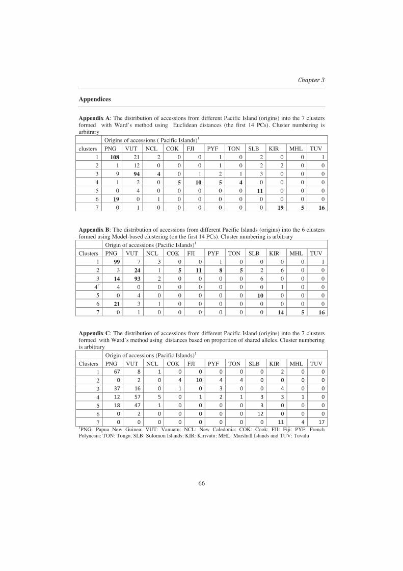
66

Appendices

Appendix A: The distribution of accessions from different Pacific Island (origins) into the 7 clusters formed with Ward’s method using Euclidean distances (the first 14 PCs). Cluster numbering is arbitrary

Origins of accessions ( Pacific Islands)1

clusters PNG VUT NCL COK FJI PYF TON SLB KIR MHL TUV

1 108 21 2 0 0 1 0 2 0 0 1

2 1 12 0 0 0 1 0 2 2 0 0

3 9 94 4 0 1 2 1 3 0 0 0

4 1 2 0 5 10 5 4 0 0 0 0

5 0 4 0 0 0 0 0 11 0 0 0

6 19 0 1 0 0 0 0 0 0 0 0

7 0 1 0 0 0 0 0 0 19 5 16

Appendix B: The distribution of accessions from different Pacific Islands (origins) into the 6 clusters formed using Model-based clustering (on the first 14 PCs). Cluster numbering is arbitrary

Origin of accessions (Pacific Islands)1

Clusters PNG VUT NCL COK FJI PYF TON SLB KIR MHL TUV

1 99 7 3 0 0 1 0 0 0 0 1

2 3 24 1 5 11 8 5 2 6 0 0

3 14 93 2 0 0 0 0 6 0 0 0

42 4 0 0 0 0 0 0 0 1 0 0

5 0 4 0 0 0 0 0 10 0 0 0

6 21 3 1 0 0 0 0 0 0 0 0

7 0 1 0 0 0 0 0 0 14 5 16

Appendix C: The distribution of accessions from different Pacific Island (origins) into the 7 clusters formed with Ward’s method using distances based on proportion of shared alleles. Cluster numbering is arbitrary

Origin of accessions (Pacific Islands)1

Clusters PNG VUT NCL COK FJI PYF TON SLB KIR MHL TUV

1

2

3

4

5

6

71PNG: Papua New Guinea; VUT: Vanuatu; NCL: New Caledonia; COK: Cook; FJI: Fiji; PYF: French Polynesia; TON: Tonga, SLB: Solomon Islands; KIR: Kirivatu; MHL: Marshall Islands and TUV: Tuvalu

T.L. Odong • J. van Heerwaarden • J. Jansen • Th.J.L. van Hintum • F.A. van Eeuwijk 2011 Statistical techniques for defining reference sets of accessions and microsatellite markers. Crop Sci 51 (6) 2401 -2411

Chapter 4

Statistical techniques for defining reference sets of accessions and microsatellite

markers

Abstract

Exploitation of the available genetic resources around the world requires information about

the relationships and genetic diversity present among genebank collections. These relations

can be established by defining for each crop a small but informative set of accessions,

together with a small set of reliable molecular markers, that can be used as reference material.

In this study, various strategies to arrive at small but informative reference sets are discussed.

For selection of accessions, we proposed Genetic Distance Optimization method (GDOpt),

which selects a subset of accessions that optimally represent the accessions not included in the

core collection. The performance of GDOpt was compared with Core Hunter, an advanced

stochastic local search algorithm for selecting core subsets. For the selection of molecular

markers, we evaluated a) backward elimination method (BE) and b) methods based on

principal component analysis (PCA). We examined the performance of the proposed

methodologies using five real datasets. Relative to average distance between an accession and

the nearest selected accession (representativeness), GDOpt outperformed Core Hunter.

However, Core Hunter outperformed GDOpt with respect to allelic richness. The BE

performed much better than other methods in selecting subsets of markers. Methods based on

PCA showed that, for practical purposes, the inclusion of the first few (two or three) PCs was

often sufficient. In order to obtain robust and high-quality reference sets of accessions and

markers we advise a combination of GDOpt (for accessions) and BE or methods based on

principal component analysis using a few PCs (for subsets of markers).

68

4.1 Introduction

Plant genetic resources stored in genebanks offer great opportunities for improving

and securing crop production, especially in marginal environments. Exploitation of

the full potential of all available genetic resources around the world requires

knowledge about the relationships relative to genetic diversity among genebank

collections stored in different centers. The relations between genebank collections

can be established by defining for each crop a small but informative set of accessions,

together with a small set of reliable molecular markers, that can be used as reference

material. Hereafter, the reference material will be referred to as “reference sets.”

A reference set of a crop should be an adequate representation of the genetic diversity

of that crop as stored in genebanks around the world. In that case, markers can be

used to place new accessions in the spectrum of current accessions. The reference sets

can also be used to connect different population genetic and quantitative genetic

studies, including association studies.

To obtain reliable reference sets, large numbers of accessions have to be genotyped

with markers. Under the auspices of the Generation Challenge Programme (GCP;

http://www.generationcp.org), large numbers of accessions of important agricultural

crops were genotyped with 15 to 50 microsatellite markers. The GCP is a broad

network of partners from international agricultural research institutes and national

agricultural research programs collectively working to improve crop productivity in

the developing world, especially environments prone to drought and having low soil

fertility, and high incidences of pests and diseases.

The general philosophy underlying the current study is that molecular markers, such

as microsatellites, can be used to represent accessions as points in a multi-dimensional

genetic space. A strategy for selecting accessions may consist of choosing accessions

in such a way that the whole of the original genetic space is covered by a pre-defined

number of accessions. With regard to molecular markers, the reference set should be

able to approximate the full genetic space by preserving the distances between the

accessions. It may be useful to identify clusters of accessions and use them as a basis

for choosing accessions in a stratified way. In addition to statistical principles,

69

molecular genetic requirements should be taken into account, especially the ease of

generating markers and marker quality.

The concept of reference sets of accessions and markers is quite similar to the concept

of forming core collections using marker information. The reference sets, unlike core

collections, place emphasis on the selection of both accessions and molecular

markers. In this case, the selected accessions are not linked to a specific genebank

collection but taken from collections assembled from many centers. Brown (1995)

referred to such a subset of accessions as synthetic core.

In this paper, various strategies to arrive at small but informative reference sets will be

discussed. For selection of accessions, we propose a method based on optimization of

the spacing of a fixed number of accessions within the genetic space; this method will

be referred to as Genetic Distance Optimization method, hereafter referred to as

GDOpt. To the best of our knowledge, currently, no method exists for the selection of

core collections that aims at obtaining a set of entries to maximize the representation

of the accessions in the whole collection. Compared to GDOpt, most existing

algorithms for selection of core collections (e.g., Mstrat (Gouesnard et al., 2001),

PowerCore (Kim et al. 2007) and Core Hunter (Thachuk et al. 2009)) pay more

attention to the content of the core collections but tend to ignore the relationships

between the selected entries and those not included in the core collection. The D-

method (Franco et al. 2006) maximizes the representation of the groups with the

assumption that the groups are known. The GDOpt aims specifically at the selection

of core entries that optimally represent accessions not included in the core collection.

For the selection of molecular markers, we examined a) a backward elimination

method and b) methods based on principal component analysis (PCA). Section 4.2

(Materials and methods) contains a description of the proposed methods and of five

datasets used for illustration in this paper. In section 4.3 (Results), the results of the

application of the proposed methodologies to five datasets will be presented.

70

4.2 Materials and Methods

4.2.1 Data

Coconut (Cocos nucifera): The coconut data consist of 1014 accessions genotyped

with 30 SSR markers. The accessions were collected from different regions of the

world (see Table 1) Coconut is a diploid, mainly outcrossing species. Most of the

accessions in this collection were described as tall; only 43 dwarf accessions mainly

from South East Asia were present. Dwarf coconuts have a high degree of self-

fertilization. More than half (19) of the 30 SSR markers used in this study have

known positions on the linkage map; they are well-spread across the genome.

Potato (Solanum species): The potato data consisted of 233 diploid accessions from

four species (S. ajanhuri (22); S. goniocalix (47); S. phureja (105) and S. stenotomum

(59)) genotyped with 50 SSR markers (see Table 1). Potatoes are mainly outcrossing,

with a substantial amount of self-fertilization. The linkage group of 42 of the 50 SSR

markers used in study is currently known.

Common bean (Phaseolus vulgaris): Genotyped with 36 SSR markers, the common

bean dataset consisted of 603 accessions with 296 being described as Andean and 307

as Mesoamerican types (see Table 1). Common bean is a self-pollinating diploid

species. Twenty-nine of the 36 SSR markers used in study belong to known linkage

groups.

Rice (Oryza sativa): The rice dataset consisted of 1998 accessions genotyped with 37

markers (see Table 1). Rice is a self-pollinating diploid species. The linkage map

positions of all 37 SSR markers used in study are known.

Chickpea (Cicer arietinum): The chickpea data consisted of 3000 accessions

genotyped with 50 SSR markers. The accessions originated from more than 60

countries (mainly from the Middle East and other parts of Asia), with germplasm

collections maintained at two international centers (ICRISAT in India and ICARDA

in Syria) and at several national gene banks (see Table 1). Chickpea is a self-

pollinating diploid species. Thirty-two of the 50 SSR markers used in study have

71

known linkage groups but the positions of the markers on the linkage map were not

available.

Table 1: Summary information on the five data sets used in this study Crop Number

of accessions

Origins of Accessions* Number of SSR markers

Coconut 1014

West Africa(32); North America(52); South Asia(62); Latin America(72); Central America & the Caribbean(109); East Africa(124); South East Asia(183); the Pacific Islands(380)

30

Potato 233

Peru(91); Colombia(80); Bolivia(44); Ecuador(16); Argentina(1) and Chile(1)

50

Common bean

603

Peru(184); Mexico(178); Guatemala(6); Ecuador(1 35); Colombia(29); Brazil(22) and others (18 countries)(94) 36

Rice 1988

India(320); Bangladesh(210); China(167); Indonesia(166); Philippines(139); Liberia(137); Sri Lanka (124); Thailand(122); USA (99); Malaysia (97); Madagascar (87); Nigeria (80) and others (250)

37

Chickpea 3000

India(820); Iran(552); Syria (183); Turkey(160); Afghanistan(147); ICRISAT collections of mixed origin(138), and Ethiopia(124) and others(876).

50

*The numbers in the parentheses indicate the number of accessions from each area of origin

72

4.2.2 Strategies for selecting representative accessions

A number of strategies for selecting subsets from large collections of accessions (with

special reference to the forming of core collections) have been proposed: MSTRAT

(Gouesnard et al. 2001), Genetic Distance Sampling (Jansen and Van Hintum, 2007),

PowerCore (Kim et al. 2007) and Core Hunter (Thachuk et al. 2009). With the

exception of Genetic Distance Sampling, all methods mentioned above apply the M-

strategy (Schoen and Brown, 1993) in some way; the M-strategy aims at maximising

the number of observed alleles of the markers in the subset of selected accessions. In

Genetic Distance Sampling, accessions are selected in such a way that selected

accessions are always a pre-defined distance (selection radius) away from each other.

This ensures that no duplicates or similar accessions are selected. A disadvantage of

the M-strategy is that it is likely to select non-representative accessions ("outliers").

None of the above methods was developed to select accessions to serve as

representatives, around which the other accessions can be positioned. In this paper, we

propose Genetic Distance Optimization (GDOpt) for selecting representative

accessions.

Genetic Distance Optimization:

The aim of GDOpt is to select a fixed number (say K) of representative accessions. It

is a form of K-medoids clustering (Kaufman and Rousseeuw, 1990), in which one

accession in each of K clusters acts as center of the cluster. Clusters are formed by

minimizing the total distance of all accessions to the nearest of the K accessions

designated as cluster centers. The current algorithm utilizes simulated annealing

(Kirkpatrick et al. 1983). To obtain a good starting point, the initial configuration of

cluster centers is provided by a modified version of Genetic Distance Sampling

(Jansen and Van Hintum, 2007). Genetic distance sampling was modified to select a

fixed number of accessions by adjusting the selection radius until the number of

accessions selected by genetic distance sampling was equal to or greater than the

required size of the reference set. If the number of accessions selected by genetic

distance sampling is greater than the intended size of the reference set, random

sampling is used to delete the extras. Eventually, the algorithm will be made

available as a procedure in the Biometris Genstat Library (http://www.biometris.nl/),

but at the moment it is available on request from the authors.

73

Comparison with Core Hunter:

In this paper, the results obtained with GDOpt are compared with those obtained with

Core Hunter (Thachuk et al. 2009). Core Hunter was selected because the authors

have demonstrated its superiority over other existing methods of core selection. In

Core Hunter, the weights attached to two optimization criteria (Modified Rogers

Distance and Shannon Diversity Index) were varied. By assigning all the weight to the

Modified Rogers Distance, Core Hunter maximizes the average genetic distance

between selected accessions, whereas by assigning all the weight to Shannon

Diversity Index, it maximizes the number of alleles in the selected accessions. The

comparison was based on two criteria: a) the distance between accessions and the

nearest entry in the reference set (representativeness) and b) the proportion of alleles

captured in a subset of a specified sample size selected by each method. This

comparison was done to show that forming core collections with the intention to

maximize either allelic richness or distances between entries (e.g., using Core Hunter

settings in this study) compromises the ability to represent the contents of the whole

collection.

The results from GDOpt and Core Hunter were also compared with those from simple

random sampling (for real data) and stratified random sampling for simulated data.

The results for the simulated datasets are presented in Appendix 1.

4.2.3 Selecting subsets of molecular markers

Criterion:

In the current context, the criterion used for comparing different methods of selecting

subsets of molecular markers is based on the preservation of genetic distances

between accessions. The key assumption is that by preserving genetic distances

between accessions, population structure (if present) will be preserved. The criterion

applied in all cases is the correlation between genetic distances between accessions

based on a subset of molecular markers and genetic distances based on all available

markers.

74

Polymorphism information content (PIC):

The PIC (Botstein et al. 1980) depends on the number and frequencies of alleles.

According to this criterion, a marker with many alleles with small frequencies is more

informative than a marker with two alleles with equal frequencies. The PIC does not

take into account the dependencies between markers. Because it is one of the most

frequently used criteria for selecting sets of molecular markers, the performance of

other methods will be compared with that based on PIC.

Methods based on Principal Component Analysis (PCA):

These methods use the dimension reduction ability of PCA to identify a subset of

molecular markers that should be retained to achieve minimum loss of information.

Recently, the use of PCA for selecting subsets of molecular markers (especially single

nucleotide polymorphisms (SNPs)) has been discussed by Paschou et al. (2007) and

Zhang et al. (2009).

Molecular markers are selected based on the weighted sum of squared loadings on all

principal components (PCs) designated as important, using the corresponding

eigenvalues as weights. The method will be referred to as ‘Weighted principal

component analysis WPCA’. The steps are (1) Perform PCA on the accession-by-

marker matrix; (2) Decide on the number of PCs to be designated as important; (3)

Calculate the weighted sum of squares of the loadings of each marker on the PCs

designated as important; (4) The markers are ranked in descending order based on

their weighted sums of squared loadings. The molecular markers are then included in

the subset based on their ranks. For weighted PCA, we compared (1) ranking based on

the first PC (WPCA1); (2) ranking based on the first two PCs (WPCA2); (3) ranking

based on the first three PCs (WPCA3) and (4) ranking based on the first 20 PCs

(WPCA20) when selecting a subset of markers.

Patterson et al. (2006) discussed the use of the Tracy-Widom distribution for

determining the number of significant principal components for SNP data. This is

done by comparing standardized eigenvalues with the Tracy-Widom distribution. If n

differentiated groups of genotypes are present in the data, one expects to find k = n-1

significant eigenvalues. However, in practice it has become standard to designate the

75

first two or three principal components as important and discard the rest without

performing any statistical test. Formal testing usually leads to many statistically

significant PCs.

Application of PCA to SSR data requires special attention. The SSR markers were

first recoded as 0, 1 or 2 based on the number of copies of the allele with frequency

closest to 0.5. The advantage of treating SSR markers in this way lies in its

simplicity. We expect the loss of information associated with coding SSR markers in

this way to be small in most cases. The SSR-marker data were recoded as described

above to reduce the information from each SSR marker into a single column, which

can then be easily related to PCs.

Backward Elimination (BE):

This method is similar to the backward elimination method used for variable selection

in multiple regression. It uses the correlation between the genetic distances (between

accessions) based on all molecular markers and the genetic distances based on a

subset of markers as the criterion for deleting markers. In a stepwise approach, at

each step, the molecular marker whose exclusion leads to the smallest reduction in

correlation between the two sets of distances is removed until a specified level of

correlation or a desired number of molecular markers is reached.

The BE method can be summarized as follows:

Step 1: Calculate the distances between accessions using all the molecular markers.

Let 0D be the matrix of those distances ( )(0 ijdD = , where ijd is the distance between

accession i and j.

Step 2: For each of the m markers, calculate the distances between accessions by

leaving out one marker at a time. Let eD ( me ,...,2,1= ) be the matrix of distances

between accessions constructed with marker e left out ( )( ijee dD = , where ijed is the

distance between accessions i and j calculated when marker e is left out). Denote er

as the correlation between 0D and eD .

76

=

< <

<

ji jiijeijeij

n

jiijeijeij

e

dddd

dddd

r22 )()(

))((

Step 3: Select marker with the largest er value, and eliminate it (the marker) from

the dataset and repeat Step 2 with the remaining markers. Each time, the maximum

value of er is recorded.

Step 4: Repeat steps 2 and 3 until either the maximum value of er reaches the

stopping value set or until the desired number of markers is achieved.

Similarity measures

In this paper, we used genetic distances (D) based on the proportion of shared alleles

(PSA) applied to the original SSR marker data and the recoded data, where D = 1 -

PSA, and

MffPSA ma

M

m

A

ama

m

/),min( 21 1

1== =

,

where maf 1 and maf 2 are the frequencies of allele a ( a =1, 2… mA ) for molecular

marker m ( m =1, 2… M ) in individuals 1 and 2, respectively. For more information

on the proportion of shared alleles as similarity measure, see Bowcock et al. (1994),

Chakraborty and Jin (1994) and Chang et al. (2009).

Other important aspects of selecting subsets of molecular markers

In addition to the statistical criteria used for selecting molecular markers, a number of

important issues should also be examined. The non-statistical issues of importance in

marker selection are quality relative to clarity and repeatability of banding pattern,

ease of automation of allele calling and genome coverage and linkage between

markers. The markers selected should be of high quality with highly reproducible

alleles.

77

4.3 Results

4.3.1 Selection of accessions

General results: In the following, representativeness is measured as average distance

between each accession to the nearest selected entry in the subset of accessions (Table

2). The GDOpt produces subsets of accessions that are much more representative

compared with Core Hunter. In all the crops, the average distance from accessions to

its nearest entry in the subset of accessions is smaller for GDOpt compared with all

settings of Core Hunter. Random sampling also performed much better than all the

different settings of Core Hunter relative to representativeness of the whole collection.

Table 2: Average distances between accessions and their nearest entry in the selected subset of accessions obtained using Genetic Distance Optimization (GDOpt), Random sampling and Core Hunter with five (CH1 – CH5) different parameter settings in terms of Modified Rogers distance (MR) and Shannon diversity index (SH). Random sampling values were obtained from 100 samples

CropMethod Coconut Potato Common bean Rice Chickpea

GDOpt 0.389 0.216 0.359 0.472 0.646

Random sampling 0.463 0.274 0.443 0.548 0.729 CH1 (MR=1.0;SH= 0.0)* 0.490 0.307 0.467 0.547 0.760CH2 (MR= 0.7;SH=0.3) 0.522 0.325 0.476 0.551 0.775 CH3 (MR=0.5;SH=0.5) 0.531 0.327 0.478 0.542 0.760 CH4 (MR=0.3;SH=0.7) 0.527 0.326 0.474 0.534 0.748 CH5 (MR=0.0;SH=1.0) 0.521 0.321 0.483 0.537 0.766 *The values in the parentheses show the different weights given to modified Rogers distance (MR) and Shannon diversity index (SH) used when selecting a subset of accessions using Core Hunter

With regard to the total number of alleles captured by subsets of 15 selected

accessions (Table 3), all parameter settings of Core Hunter performed better than

GDOpt. However, major differences were found in the retention of alleles with

different frequencies (see Fig. 1). For ease of interpretation, we have classified alleles

into three categories based on their frequencies ( p ): a) common alleles-CA

( 05.0p ) b) rare alleles-RA ( 05.0005.0 <p ) and c) very rare alleles-VRA

( 005.0<p ). The proportion of common alleles captured by GDOpt and different

settings of Core Hunter were comparable. For all five crops, subsets of 15 accessions

selected using GDOpt performed well in capturing common alleles. With the

78

exception of chickpea, subsets selected via GDOpt captured more than 85% of all

common alleles. In potato and common bean, subsets of accessions obtained by

GDOpt showed a higher frequency of common alleles compared with subsets of

accessions obtained by the different settings of Core Hunter. Core Hunter performed

much better than GDOpt in capturing rare and very rare alleles. However, with

simulated data, GDOpt performed better than Core Hunter with all the weights given

to Modified Roger’s distance relative to proportion of captured alleles (see Appendix

1).

Table 3: Numbers of alleles in the whole datasets and proportions of alleles in subsets of 15 accessions obtained using Genetic Distance Optimization, Random sampling and Core Hunter with five (CH1 – CH5) different parameter settings in terms of Modified Rogers distance (MR) and Shannon diversity index (SH). Random sample values were obtained from 10 samples

Crop Method Coconut Potato Common bean Rice Chickpea

Whole dataset 469 367 1089 566 1605 GDOpt 0.422 0.635 0.255 0.339 0.318 Random sampling 0.430 0.554 0.254 0.344 0.264 CH1 (MR=1.0;SH= 0.0)* 0.388 0.700 0.298 0.426 0.318 CH2 (MR= 0.7;SH=0.3) 0.527 0.796 0.332 0.459 0.338 CH3 (MR=0.5;SH=0.5) 0.563 0.820 0.341 0.466 0.336 CH4 (MR=0.3;SH=0.7) 0.569 0.837 0.346 0.463 0.333 CH5 (MR=0.0;SH=1.0) 0.569 0.839 0.350 0.482 0.343

*The values in the parentheses show the different weights given to modified Rogers distance (MR) and Shannon diversity index (SH) used when selecting a subset of accessions using Core Hunter

79

Fig 7: Proportions of alleles in different classes in the whole dataset (Whole_Col) and in subsets of 15 accessions obtained using Genetic Distance Optimization (GOpt), random sampling and different parameter settings for Core Hunter (CH1-RD(1)SH(0); CH2-RD(0.7)SH(0.3); CH3-RD(0.5)SH(0.5); CH4-RD(0.3)SH(0.7); CH5-RD(0)SH(1)). The parameter settings refer to weights assigned to Modified Rogers Distance (RD) and Shannon diversity Index (SH). Classes are based on the frequencies of the alleles in whole collection (Common alleles-CA ( 05.0P ); Rare alleles-RA

( 05.0005.0 <p ) and Very rare alleles-VRA ( 005.0<p ))

4.3.2 Selection of markers

General Results: In the following, the preservation of pairwise distances between

accessions by a subset of SSR markers is measured by the correlation between the

distances based on the subset of SSR markers and the distances based on the whole set

of SSR markers (Table 4).

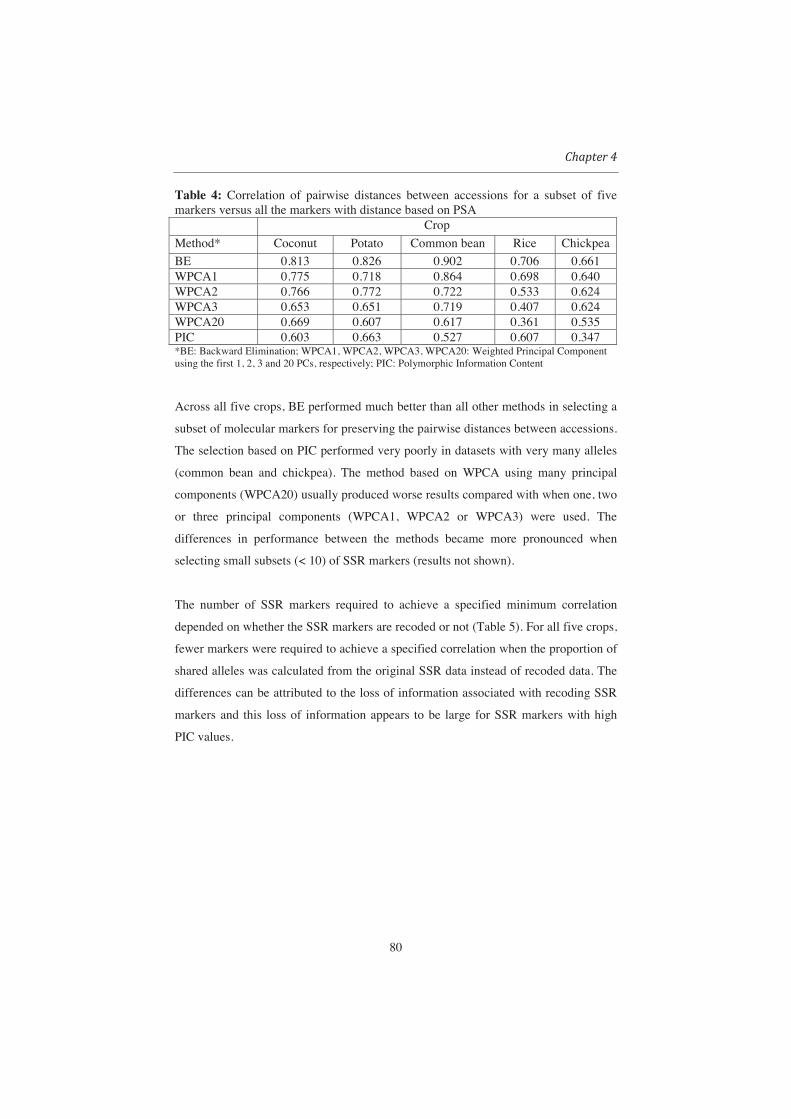
80

Table 4: Correlation of pairwise distances between accessions for a subset of five markers versus all the markers with distance based on PSA

Crop

Method* Coconut Potato Common bean Rice Chickpea

BE 0.813 0.826 0.902 0.706 0.661 WPCA1 0.775 0.718 0.864 0.698 0.640 WPCA2 0.766 0.772 0.722 0.533 0.624 WPCA3 0.653 0.651 0.719 0.407 0.624 WPCA20 0.669 0.607 0.617 0.361 0.535 PIC 0.603 0.663 0.527 0.607 0.347 *BE: Backward Elimination; WPCA1, WPCA2, WPCA3, WPCA20: Weighted Principal Component using the first 1, 2, 3 and 20 PCs, respectively; PIC: Polymorphic Information Content

Across all five crops, BE performed much better than all other methods in selecting a

subset of molecular markers for preserving the pairwise distances between accessions.

The selection based on PIC performed very poorly in datasets with very many alleles

(common bean and chickpea). The method based on WPCA using many principal

components (WPCA20) usually produced worse results compared with when one, two

or three principal components (WPCA1, WPCA2 or WPCA3) were used. The

differences in performance between the methods became more pronounced when

selecting small subsets (< 10) of SSR markers (results not shown).

The number of SSR markers required to achieve a specified minimum correlation

depended on whether the SSR markers are recoded or not (Table 5). For all five crops,

fewer markers were required to achieve a specified correlation when the proportion of

shared alleles was calculated from the original SSR data instead of recoded data. The

differences can be attributed to the loss of information associated with recoding SSR

markers and this loss of information appears to be large for SSR markers with high

PIC values.

81

Table 5: Numbers of selected markers required to achieve a minimum correlation of 0.85 between distances between accessions based on markers selected using different methods and distances between accessions based on all markers. The numbers in the parenthesis is obtained when the distances between accessions were based on SSR data recorded as 0,1 or 2.

Crop

Method* Coconut Potato Common bean Rice Chickpea

BE 7(12) 6(13) 2(3) 13(18) 16(23) WPCA1 9(16) 16(23) 2(2) 13(18) 18(26) WPCA2 9(14) 11(24) 7(11) 13(18) 17(26) WPCA3 11(15) 15(24) 9(12) 15(19) 17(24) WPCA20 11(16) 15(28) 11(14) 20(22) 21(25) PIC 14(20) 18(31) 13(17) 18(22) 40(40) *BE: Backward Elimination; WPCA1, WPCA2, WPCA3, WPCA20: Weighted Principal Component using the first 1, 2, 3 and 20 PCs, respectively; PIC: Polymorphic Information Content

Evaluation of subsets of five SSR markers indicated that BE and WPCA-based

methods tended to select markers whose major alleles had frequencies close to 0.5

(Table 6). These SSR markers separated major groups of accessions. The PIC

criterion favored SSR markers with very many alleles. These SSR markers

differentiated between individual accessions or small groups of accessions thus played

a minimal role in separating major groups.

Table 6: Average frequencies of major alleles in a subset of five SSR markers selected by different methods

Crop Method* Coconut Potato Common bean Rice ChickpeaBE 0.501 0.511 0.484 0.311 0.420 WPCA1 0.515 0.566 0.515 0.459 0.435 WPCA2 0.562 0.541 0.320 0.411 0.461 WPCA3 0.388 0.482 0.455 0.440 0.461 WPCA20 0.367 0.428 0.386 0.414 0.209 PIC 0.241 0.357 0.122 0.201 0.070 *BE: Backward Elimination; WPCA1, WPCA2, WPCA3, WPCA20: Weighted Principal Component using the first 1, 2, 3 and 20 PCs, respectively; PIC: Polymorphic Information Content

82

Crop-specific results

Coconut: The best method for selection of a subset of markers was BE, followed by

WPCA1 and WPCA2 (see Fig 2). For example, when distances were based on PSA,

using the original SSR marker data we only required seven out 30 markers using BE,

compared with 14 using PIC criterion to achieve a correlation of 0.85. The results

obtained for WPCA3 and WPCA20 were quite similar to random sampling of marker

subsets but better than those for PIC. A similar pattern in the number of molecular

markers required to achieve a correlation of 0.85 was observed when distances were

calculated using the recoded data, except that the numbers of required markers were

much higher.

Potato: BE outperformed all other methods in selecting a subset of molecular markers

(see Fig. 2). When pairwise distances between accessions were calculated using PSA

based on the original SSR marker data, we only needed six out of 50 markers to

achieve a correlation of 0.85, which is less than half the number required by other

methods. For the number of molecular markers needed to achieve a correlation of

0.85 (with the exception of WPCA2), the performances of the other methods were

quite similar. Only BE, WPCA1 and WPCA2 performed better than random selection.

Common bean: For common bean, a much greater difference in the performance of

BE, compared with the other methods (except WPCA1), was found than for the other

crops, especially in subsets of markers of small size (see Fig. 2). The PIC performed

very poorly in this dataset. The BE and WPCA1 required only two out 33 of SSR

markers to achieve a correlation of 0.85 compared with 13 markers for PIC. The

performance of WPCA20 was quite similar to that of PIC.

Rice: The BE performed better than the other methods, except WPCA1 (see Fig. 2).

The performances of BE, WPCA1 and WPCA2 were very similar for subsets of

markers with sizes greater than 10. For subsets of markers of sizes less than 10,

random selection of markers performed much better than WPCA3 and WPCA20.

With the exception of BE and WPCA1, the method based on PIC performed better

than other methods for subsets of size less than 5. When correlation was based on

recoded SSR data, WPCA20 and PIC required the same number of markers (22) to

achieve a correlation of 0.85.

83

Chickpea: Although BE method performed better than all the other methods, the

differences in performance were not prominent, especially with WPCA-based

methods (see Fig. 2). The selection based on PIC performed very poorly compared

with the other methods. The PIC required 40 out of 50 markers to achieve a

correlation of 0.85. In this case, randomly selecting a subset of SSR markers produced

much better results than PIC.

4.4 Discussion and Conclusions

Understanding the current status of genetic diversity and finding links between

genetic resources stored in different institutions are essential for a successful,

worldwide exploitation of genetic resources for crop improvement. The concept of

reference sets of accessions and markers provides an efficient way to relate new

materials to existing ones and set up different crop-specific study panels that can be

used by plant breeders worldwide, with just a few representative accessions and a few

84

molecular markers covering the genetic diversity in each crop. For example, selected

accessions can be used for creating the so-called MAGIC (Multiparent Advanced

Generation Inter-Cross) population, which can be used for QTL analysis. Kover et al.

(2009) demonstrated the utility of MAGIC population in improving the precision of

QTL mapping.

In this study, representative accessions were selected using GDOpt, which aims at

optimizing the spacing of a fixed number of accessions within the genetic space

defined by all available markers. By performing selection and clustering of accessions

simultaneously, this method can avoid the tedious process of determining population

structure of the collection. Determination of population structure is quite challenging,

especially in the case of germplasm collections where most often no clearly defined

groups exist (Odong et al. 2011). In highly diverse collections, it may only be possible

to isolate subsets of closely related individuals rather than obtaining large

homogenous groups (Hamblin et al. 2007). It is from these closely related individuals

that GDOpt selects a representative. Results from simulations have shown that if

groups are known, stratified sampling does give improvement over simple random

sampling, but its performance is still worse than that of GDOpt (Appendix 1).

However, in situations where distinct groups of accessions exist (e.g., the Andean and

Mesoamerican types of common beans), the selection can be performed separately for

each group. Most methods that aim at optimizing either allelic richness or maximum

genetic distances between selected accessions are quite capable of covering the full

range of genetic diversity, including extremes, but may not produce representative

subsets of accessions. For example, by simply selecting extremes, it would be

possible to produce a subset with maximum genetic distances between accessions or

maximum number of alleles although the selected accessions are not fully

representative of the whole collection. Moreover, according to Zhang et al. (2010), the

majority of very rare alleles would not contribute to the genetic diversity needed to

develop elite cultivars and therefore their inclusion in the core collection may not be

worthwhile. Some scientists (Allard, 1992; Frankel et al. 1995) have argued that less

frequent alleles only occasionally affect quality or other traits and are generally

unlikely to be of future use. In a situation where a representative subset is required,

GDOpt has great advantages over all other methods, as shown in this study.

85

One of the key challenges in selecting representative sets of accessions based on

distances between accessions is the effect of (random) errors in the data. In general,

(random) errors will inflate dissimilarities between individuals, with smaller

dissimilarities being relatively more inflated than larger ones. The inflation of

dissimilarities consequently results in an overall greater dispersion of accessions in

the genetic space, making it more difficult to obtain representative sets of accessions.

The use of SSR markers with very many alleles (and consequently high PIC values)

aggravates this problem. It is thus clear that if we are interested in a stable relationship

between accessions, then the distances obtained from all the available markers and/or

all alleles may be unsuitable. Markers with very high PIC (or very many alleles), in

addition to inflating the distances between accessions, are likely to provide

inconsistent relationships because of the fact that some of the alleles are as a result of

misreading bands and are not repeatable. A much more stable relationship (distance)

between accessions can be obtained by discarding some markers. Our results show

that for all the five crops, 10 or more markers can be discarded without much

distortion of pairwise distances between accessions. Another alternative for obtaining

a stable relationship between accessions or group of accessions would be to calculate

distances using important PCs, but additional studies are needed.

For the selection of subsets of molecular markers, we have shown that if one is

interested in selecting a subset that preserves pairwise distances between accessions,

BE provides the best option. The BE tends to remove markers with very many alleles

and lots of missing values because they tend to contribute less to pairwise distances

between accessions. The first markers included in the subset using BE mainly separate

the major groups present in the data but could have the weakness of not differentiating

well between accessions within groups. For example, for the common bean data, only

two markers are required to achieve a correlation of 0.85 and those two markers

separate Mesoamerican and Andean types quite well. A similar situation was

observed for coconut where the first five markers separated accessions associated with

the Pacific Ocean from those associated with Indian and Atlantic Oceans.

Simulations (results not shown) indicated that the correlation between pairwise

distances between accessions based on a subset of markers and distances based on the

entire set of markers depended on the level of group structure in the data. The stronger

the group structure, the fewer the number of markers required to preserve the pairwise

86

distances between accessions. The performance of BE could be improved by

performing marker selections in two steps, i.e., first perform BE based on the whole

dataset and subsequently perform it within the major groups. For rice and chickpea,

the difference in performance between BE and other methods was smaller compared

to common bean, coconut and potatoes. This could be attributed to nature of group

structure present in these datasets. Both multidimensional scaling and cluster analysis

showed the presence of strong structure that was consistent with passport data in the

three datasets (common bean, coconut and potato), which indicated a large difference

between BE and other methods of selection of subset of markers compared to rice and

chickpea.

The performances of the PCA-based methods were quite good and in some cases

comparable with that of BE. Our study revealed one interesting aspect about the

number of important principal components to be included in the selection process. In

all our datasets, the first few (1 to 3) principal components appeared to be sufficient.

For most datasets, the eigenvalues revealed a big difference between the first two or

three principal components compared with the rest; which made the contribution of

the later PCs of minor importance. The practice of determining the number of

important PCs through rigorous statistical testing most often leads to inclusion of too

many principal components, which in turn introduces noise. A recent study by Lee et

al. (2009) noted a negative effect of including all significant PCs when performing

distance-based cluster analysis.

Subsets of markers selected using PIC performed very poorly in preserving pairwise

distances between the accessions, especially with common bean and chickpea. The

poor performance with common bean and chickpea could be attributed to the poor

quality of the data. Both datasets contained many markers with a very large number of

alleles with more than 50% of the alleles having frequencies of less than 0.01 (see

Appendix 2 for diversity statistics of the SSR markers for common bean data used in

this study). In both crop species, the average frequency of major alleles for the five

SSR markers with the highest PIC is much smaller compared with subsets formed by

BE and PCA-based method. A large of number of alleles with frequencies of less

than 0.01 could be because of poor binning of alleles. The presence of error (random)

in the data was thus more likely to affect selection of markers based on PIC compared

with BE and WPCA-based methods. The BE and WPCA-based methods (especially

87

WPCA1, WPCA2 and WPCA3) were more robust for detecting errors because those

methods only picked out the key features of the data. Although PIC is the most

common criterion used for selection of molecular markers, we have shown in this

study that it performed poorly with respect to preserving major relationships between

groups of individuals. Because PIC measures genetic diversity within a population, its

poor performance with respect to identifying major features in the data is not

surprising.

When SSR markers were recoded, the difference in performance between the different

methods was smaller compared with the results obtained using the original SSR

marker scores. This may be because of a loss of information; forcing alleles into just

two categories (allele with frequency closest to 0.5 versus others) tends to smooth out

differences between accessions. It is clear from literature that one needs more bi-

allelic markers to achieve the same level of genetic distance accuracy as a set of

multi-allelic markers, such as microsatellites (see Laval et al. 2002). As noted from

the results in this study, recoding affected markers with a high PIC much more than

other markers. The correlation between distances between the accessions based on the

original SSR markers and distances based on recoded SSR markers indicated some

loss of information. The correlations for chickpea, coconut, rice, common beans and

potatoes were 0.42, 0.69, 0.71, 0.82 and 0.88, respectively. The low correlation for

chickpea (0.42) is an indication that recoding SSR data can sometimes lead to a

substantial loss of information, and therefore it should be applied cautiously. Other

methods, such as performing PCA on allele frequencies from each SSR marker

separately and later combining the information across all markers, can be explored.

One of the key advantages of BE and PCA-based method is that the selected

molecular markers are likely to be independent. For PIC, unless sets of markers on

which selection is done are known to be independent, there is no guarantee that the

selected markers will be independent. For the datasets used in this study, several of

the markers provided were on different linkage groups and those for which the

positions on the chromosomes were given showed wide spacing between the markers

(independence).

88

It is clear from our study that using both BE and PCA-based methods, several good

subsets of markers can be obtained. Other (quality aspects) of the chosen molecular

markers (e.g., the possibilities for multiplexing) can be used to identify the most

appropriate set. In the same way, alternative sets of accessions also exist and suitable

accessions can be selected to replace less desirable ones. For example, accessions

with missing values or those known to have propagation problems can be replaced.

Discussion with genebank curators, crop specialists and laboratory technicians can

provide information that can be used as a basis of determining which of the selected

accessions and molecular markers should be retained or dropped. The use of

multivariate statistical techniques, such as multidimensional scaling, can assist in

visualizing the selected accession in the space defined by the selected subset of

markers.

In summary, for the selection of subsets of both accessions and markers, several

methods exist, each with their own advantages and disadvantages, i.e., there is no

perfect core collection suitable for all purposes. Although GDOpt performs very well

with respect to representativeness of non-selected accessions, its performance with

respect to maximizing genetic diversity parameters, such as allelic richness or

distances between selected accessions, is slightly compromised – i.e., there is a trade-

off. Methods such as Mstrat (Gouesnard et al., 2001) PowerCore (Kim et al. 2007)

and Core Hunter (Thachuk et al. 2009) should be used when the interest is in selecting

subsets of accessions by maximizing diversity parameters, such as allelic richness or

distance between entries in the core collection. For the selection of subsets of

molecular markers, both BE and methods based on the first few (two or three) PCs

gave rise to subsets of markers that preserved the major structure in the data but may

have performed poorly for discriminating between individuals within the groups

compared with markers with a high PIC.

89

Appendices

Appendix 1

Result of simulated data

a)

b)

Figure 3: Boxplot of a) distance between each accession and the nearest entry in the core collection (A-NE distance) and b) Proportion of alleles captured by core collections (of size 15) obtained by GDOpt, different settings of Core Hunter (CH-0/1, CH-0.7/0.3, CH-0.5/0.5, CH-0.3/0.7, CH-0/1), Random sampling (Random) and Stratified Random sampling (StrRandom) from 10 simulated data sets. For both random and stratified sampling, for each data set sampling was performed 100 times.

90

Appendix 2

Table 6: Values of diversity statistics for each molecular marker – Common beans

Marker No. of Alleles Frequency of Major alleles No. of Genotypes Gene Diversity Heterozygosity PIC

PV_at001 121 0.0540 181 0.9814 0.6945 0.9810

BM187 95 0.1317 137 0.9533 0.3034 0.9516

GATS91 48 0.0825 79 0.9523 0.0846 0.9502

BM143 65 0.1594 109 0.9394 0.1299 0.9366

BM156 62 0.1817 93 0.9310 0.1044 0.9276

BMd01 40 0.1491 99 0.9253 0.7059 0.9208

BM200 58 0.1706 90 0.9213 0.1983 0.9166

BM188 49 0.1653 91 0.9191 0.8152 0.9140

PV_ctt001 23 0.1690 38 0.8860 0.0716 0.8752

BM141 38 0.2527 75 0.8740 0.2602 0.8642

BM175 39 0.2888 58 0.8707 0.0510 0.8616

BM183 41 0.2755 62 0.8695 0.1216 0.8589

BM172 47 0.3489 83 0.8580 0.1470 0.8527

BM160 59 0.3705 83 0.8497 0.0936 0.8460

BM205 19 0.3296 37 0.8219 0.2480 0.8035

BM139 27 0.4534 46 0.7679 0.0769 0.7564

BM201 16 0.3004 29 0.8152 0.0576 0.7920

BMd16 22 0.3096 35 0.7798 0.1743 0.7481

PV_ag003 12 0.3153 17 0.7685 0.0196 0.7329

BMd15 22 0.3476 33 0.7423 0.3111 0.6996

BMd18 15 0.3877 19 0.7111 0.3475 0.6663

BM149 10 0.5764 15 0.6328 0.0238 0.6086

PV_cct001 14 0.5000 17 0.6533 0.0724 0.6002

BMd08 14 0.5114 18 0.6716 0.0207 0.6345

BMd20 10 0.5397 13 0.6412 0.0146 0.5997

BMd47 10 0.4615 14 0.6554 0.0243 0.5952

BMd17 9 0.4892 12 0.6390 0.0784 0.5735

AG01 10 0.5780 17 0.5971 0.1951 0.5499

BMd02 12 0.5539 15 0.6012 0.0294 0.5420

PV_at003 14 0.4567 19 0.6056 0.1333 0.5258

BMd46 7 0.4930 10 0.5362 0.0099 0.4286

GATS54 9 0.6815 11 0.4555 0.0643 0.3811

BMd51 3 0.9894 3 0.0211 0.0000 0.0209

Only summary for 33 SSR markers shown

This chapter is submitted (under revision) to Theoretical and Applied Genetics as: T.L. Odong J. Jansen F.A. van Eeuwijk -- T.J.L. van Hintum Quality of Core Collections for Effective Utilization of Genetic Resources Review, Discussion and Interpretation

Chapter 5

Quality of core collections for effective utilization of genetic resources

Review, discussion and interpretation

ABSTRACT

Defining proper criteria for evaluating the quality of core collections is a prerequisite

for selecting high-quality cores. However, a critical examination of the different

methods used in literature for evaluating of the quality of core collections shows that

there are no clear guidelines on the choices of quality evaluation criteria and as a

result, inappropriate analyses are sometimes made leading to many false conclusions

being drawn regarding the quality of core collections and the methods to select them.

The choice of criteria for evaluating core collections appear to be based mainly on

criteria being used in earlier publications rather than on the objectives of the core

collection. In this study, an insight in the different criteria used for evaluating core

collections is provided. We also discuss the different types of core collections and

relate each type of core collection to possible evaluation criteria. Two new criteria

based on genetic distance are introduced. The consequences of the different

evaluation criteria are illustrated using simulated and experimental data. We strongly

recommend the use of the distance-based criteria since they not only allow the

simultaneous evaluation of all variables describing the accessions, but they also

provide intuitive and interpretable criteria, as compared with the univariate criteria

generally used for the evaluation of core collections. The results presented allow

genebank curators and researchers to make informed choices when creating,

comparing and using core collections.

92

5.1 Introduction

Ex-situ germplasm collections have increased enormously in number and size over the

last three to four decades as a result of global efforts to conserve plant genetic

resources for food and agriculture. The large sizes of these collections complicate the

characterization, evaluation, utilization and maintenance of the conserved germplasm.

The approach of forming core collections (core sub-sets) was introduced to increase

the efficiency of characterization and utilization of collections stored in the gene

banks, while preserving as much as possible the genetic diversity of the entire

collection (Frankel, 1984; Brown 1989). Frankel (1984) defined a core collection as a

limited set of accessions representing, with minimum repetitiveness, the genetic

diversity of a crop species and its wild relatives. From the original definition, several

operational definitions have been coined (see Brown, 1995 and Van Hintum et al.

2000).

Core collections have many roles to play in the management and use of genetic

resources. Gene bank curators have the responsibility for conservation, regeneration,

safety duplication, documentation, evaluation and characterization of the genetic

resources in their collections. These activities often require them to make choices or

set priorities among accessions because of limited resources (Brown, 1995). Because

a core collection is smaller in size compared to the whole collection, it enables some

operations of the genebank, such as evaluation, to be handled more efficiently and

effectively. The limited size of a core is key to its manageability, and in many cases

the representation of the collection’s diversity enables the core to function as a

reference set of accessions for the whole collection (Brown and Spillane, 1999).

Since the inception of the idea of core collections over two decades ago, a body of

literature on the theory and practice of core collections has accumulated. Very many

approaches for selecting core collections have been proposed and used (e.g. M-Strat

(Gouesnard et al. 2001), Genetic distance sampling (Jansen and van Hintum 2007),

Power Core (Kim et al. 2007) and Core Hunter (Thachuk et al. 2009)). In comparing

the options for assembling a core collection, one of the challenges is to decide on the

evaluation criteria for the quality of the result. Various criteria for determining the

suitability of a core collection have been suggested in the literature, yet very little

93

attention has been given to the analysis of these quality criteria. In fact every

researcher appears to have his/her own criteria for the evaluation of core collections.

There is a need to clearly define criteria for the evaluation of the quality of core

collections and to determine the conditions under which these are suitable. For

example, a core subset formed for the purpose of capturing rare or extreme traits (e.g.

high resistance to pest or high yield) should be evaluated differently from one formed

with the intention of representing an overview of the pattern of genetic diversity in

the collection. By the pattern of genetic diversity we refer to the differences in the

genetic constitutions of the accessions which have been accumulated as a result of

natural processes, species characteristics and historical events.

In this paper, we will i) discuss the different types of core collections and proposed

criteria suitable for quality evaluation of each type of core collection ii) discuss the

different criteria used in the literature for evaluating the quality of core collections and

relate each criterion to the different types of core collections iii) use real data sets

(molecular marker data) to illustrate the performance of the proposed quality

evaluation criteria with respect to the different types of core collections. The outcome

of our study will allow researchers and curators to make informed choices from a set

of alternative approaches.

5.2 What is a good core collection?

One of the key goals of defining a core collection is efficient utilization of available

genetic resources and this is best achieved by having clear objectives in mind when

selecting entries for the core (Mackay, 1995). The answer to the question “what is a

good core collection” therefore depends on the objectives for making the core. This

can be “storing as much variation as possible”, “optimizing the chance of finding a

new allele” but also “obtaining a few accessions that represent the spectrum of

phenotypes in the collection”. A second question is how to measure quality, and this

will depend on the type of data available for evaluation.

According to Brown (1989), a good core collection should have no redundant entries

(an entry is an accession included in the core), represent the whole collection with

94

regards to species, subspecies and geographical regions and should be small enough to

be easily managed. It was suggested by Marita et al. (2000) that selection of core

collections can be performed with two general purposes i) maximizing the total

genetic diversity(as sometimes favoured by taxonomists and geneticists) and ii)

maximizing the representativeness of genetic diversity in the whole collection (as

sometimes favoured by plant breeders). Accordingly, maximizing the

representativeness of genetic diversity implies the inclusion of broadly adapted and

heterotic materials containing ‘generalist’ alleles in a core collection. Earlier, Galwey

(1995) stated these two purposes of core collections in a slightly different way as: (i)

maximizing the representativeness of the full range of variation in whole collection;

(ii) maximizing the representativeness of the pattern of variation in the whole

collection.

There is also an aspect of balance between representing total diversity and the

usefulness of the core to the intended user (Brown 1995). This can be illustrated with

some examples. If a breeder searches for a particular trait, it is likely that the best core

collection should contain relatively more material from the primary genepool as

compared to the secondary genepool, irrespective of the amount of diversity in it, and

within the primary genepool there will be a strong preference for material in an

adapted genetic background. If a core collection is created in the search for new

resistances, the part of the genepool that in the past has shown to contain resistances

should obviously be overrepresented. This implies that the user is often not primarily

interested in maximising diversity per sé (which would result in core collections with

mainly wild and exotic material), but rather in optimising the chance of finding what

he/she is looking for in material which is relatively easy to use in, say, a breeding

programme. To achieve this, the selection of a core collection often starts with

stratifying accessions into homogeneous groups, followed by an arbitrary

determination of the number of accessions to be selected from each group, the so-

called allocation. When a core collection is being formed for a specific user, the

stratification and allocation process can be used to ensure that accessions from (a)

particular group(s) (e.g. primary gene pool, modern varieties or Ethiopian landraces)

are given more priority than justified by the genetic variation contained in that group.

Since this stratification and especially the allocation process is sometimes arbitrarily

defined by curators or users, it is difficult to incorporate this aspect into quality

95

criteria. The rest of this paper will therefore concentrate on non-stratified groups of

accessions. However, it should be noted that when grouping of accessions is

necessary and/or when the groups can be appropriately determined, the quality

criteria should be applied within the different groups.

From the literature, it is not clear how to relate the purpose of the core collections

with the various quality evaluation criteria, and only very few authors have attempted

this (e.g. Thachuk et al. 2009). Based on the purposes of core collections as suggested

by Galwey (1995) and Marita et al. (2000), we have identified three broad types of

core collection which will be discussed in the next section.

5.3 Types of Core Collections

Based on the purposes for which they are formed core collections can generally be

classified into three categories. In defining the types of core collections, the term

accessions refers to elements that constitute the whole collection (population) and

entries are elements of the core collection (sample). Since the core collection is a

selection from the whole collection, all entries are accessions, but only few accessions

are entries.

Type 1: A core collection representing the individual accessions of the whole

collection (CC-I).

Implication: each accession of the whole collection is represented by an entry of the

core collection (usually by the closest entry).

This type of core collection (CC-I) aims at a uniform representation of the original

genetic space, with equal weights across this space and is the most intuitive way of

looking at core collection (see Fig 1). A core collection of type CC-I is especially

suitable, for situations requiring an overview of the diversity of the accessions of the

whole collection. Core collections formed for the purposes of maximizing the

representativeness of genetic diversity as suggested by Marita et al. (2000) can be

placed in type CC-I.

96

Type 2: A core collection representing the extremes of the whole collection (CC-X).

Implication: the diversity of the traits of the entries of the core collection is

maximized.

A core collection of type CC-X is geared towards representing the ranges of

phenotypes or alleles of the whole collection. A good core collection of type CC-X

has entries that are as different as possible from each other. A core collection

representing the total genetic diversity, as suggested by Marita et al. (2000), can be

considered as a core collection of type CC-X.

Type 3: A core collection representing the distribution of accessions of the whole

collection (CC-D).

Implication: the distributions of all relevant traits with regard to the entries of the core

are similar (in terms of mean, variance, quartiles, frequencies) to those of the whole

collection.

This core collection of type CC-D is hardly ever of interest; only if the aim is to give

an overview of a the composition of the whole collection using only a part of the

collection, this type should be considered. This type of core collection will be

obtained by maximizing the representativeness of the pattern of variation of traits in

the whole collection, as suggested by Galwey (1995).

Although a CC-D core collection is hardly of interest, the criteria used for evaluating

most core collections in the literature suggest that most core collections are of type

CC-D (e.g. annual medicago (Diwan et al. 1994), sesame core collection - China

(Xiurong et al. 1998), Iberia Peninsula common bean (Rodino et al. 2003), groundnut

(Upadhyaya et al. 2003), peanut (Valencia) (Dwivedi et al. 2008), USDA soybean

core (Oliveira, et al. 2010) ).

The different types of core collections have been illustrated graphically using a

multimodal univariate distribution for the whole collection (Fig 1).

97

Fig 1: A. Multimodal trait distribution of for whole collection; B. Distribution of the same trait for a collection of type CC-I; C. Distribution of the same trait for a core collection of type CC-X ; D. Distribution of the same distribution for a collection of type CC-D

5.4 Quality criteria for evaluating core collections

The process of evaluating a core collection usually involves a comparison with the

whole collection from which it has been obtained, or a comparison with alternative

core collections. This requires clear and objective criteria for assessing the quality of

the different types of core collections.

Irrespective of the type of core collection and the quality criterion used, the evaluation

of quality should be based if possible on data that were not used in the selection of the

core (van Hintum et al. 2000). This might sound like an obvious statement, but it is

very often neglected (e.g. Tai and Miller 2001 and Wang et al. 2007). For example,

one has a dataset of 1000 accessions each genotyped with 50 markers, and the

objective is to create a core collection of 20 entries with maximal allelic richness. If it

would concern only the current 50 markers, this would be a simple optimisation

problem. However, the question is, “what if the core collection should also be ‘allelic

rich’ for all loci that were not genotyped?” One option would be to use half the

98

markers for creating core collections using different methods, and the other half for

evaluating the quality of the result of each method (for a good examples see Mckhann

et al. (2004), Ronfort et al. (2006) and Balfourier et al. (2007)). Once the best strategy

has been determined this strategy could then be used on the entire set of markers to

create the final core collection. Since often molecular data will be used to select a core

that is also supposed to optimize the phenotypic diversity, relevant phenotypic traits

should be used for the validation.

In this article, we place emphasis on evaluation criteria based on genetic distances

between accessions. The main advantage of using genetic distance for evaluation of

core collections is that unlike the other criteria used in literature which handle one

variable at a time, all the variables are used simultaneously. It is also easier and more

intuitive to link distances to the concept of genetic diversity.

Evaluation of type CC-I

A good criterion for evaluation CC-I core should relate each accession of the whole

collection with the entries of the core collection. For CC-I, we proposed criteria based

on distances between each accession in the whole collection and the nearest entry in

the core collection (A-NE) (see Fig 2).

Fig 2: A) Eight accessions (1,2,..,8) in a 2D space with all pairwise distances (the distance between accession n and m is indicated as Dn-m). B) The three selected entries (highlighted accessions) based on the A-NE criterion, minimising the average distance between each accession and it nearest neighbouring entry (D1-2 + D2-2 + D3-3+ D4-2 + D5-6 + D6-6 + D7-6 + D8-6)/8

99

Average distance between each accession and the nearest entry (A-NE) (Odong et al

2011b): In this case, the distance between each accession and the nearest entry in the

core is calculated and averaged over all the accessions. For the selected accessions

(entries) these distances are taken as zero (they are closest to themselves). For

example, the value A-NE for Fig 2 is given as

Where the distance between accession n and m is indicated as Dn-m.

For core collections of type CC-I, the value of A-NE should be as small as possible;

the maximum representation (A-NE = 0) is obtained when each accession is

represented by itself or by an identical duplicate accession in the core. In core

collections that optimize the values of A-NE (CC-I type of core), the accessions

selected as entries tend to be centres of clusters(groups) rather peripheral objects (see

Fig 4).

Evaluation of type CC-X

A good criterion for a core collection of type CC-X (representing the extreme values)

should be able to quantify differences between entries of the core collection as well as

being able to measure the inclusion or exclusion of accessions with extreme traits in

the core. The most intuitive criteria for determining differences between entries in the

core collection are those criteria based on pair-wise distances. The exclusion or

inclusion of accessions with extremes values in the core can be assessed using

frequencies of traits or alleles captured (see Thachuk et al. 2009). Below we propose a

new criterion based on distances between an entry and the nearest neighbouring entry

(E-NE) and compare it with criteria based on average pair wise distances between all

entries.

8

)( 6867666524332221 +++++++=

DDDDDDDDNEA

100

Fig 3: A) Eight accessions (1,2,..,8) in a 2D space with all pairwise distances (the distance between accession n and m is indicated as Dn-m). B) The three selected entries (highlighted accessions) based on the E-NE criterion maximizing distances between each entry and the nearest neighbouring (D1-3 + D3-1 + D7-1)/3

Average distance between each entry and the nearest neighbouring entry (E-NE):

According to this criterion (E-NE), a good core collection is one that maximizes the

average distance between each entry and the nearest neighbouring entry in the core

collection. For this criterion, each entry should be as different as possible from the

most similar entry. This avoids selecting a few clusters of similar accessions at the

extreme ends of the distribution, that might occur if one chooses a set of entries that

maximizes the average of all pair-wise distances between the entries in the core (E-

E) (see Fig 4). Using example in Fig 3, if accessions 1,3 and 7 are selected as entries

in the core collection, and if 1 is the nearest neighbouring entry to both 3 and 7

(reverse is also true) then E-NE is given as

3

)( 171331 ++=

DDDNEE

where the distance between accession n and m is indicated as Dn-m.

Average genetic distances between entries (E-E): Maximizing the average genetic

distance between entries of a core collection has been suggested as a desired quality

criterion for evaluating core collections intended for plant breeders (Franco, 2006,

Thachuk et al. 2009). Using example in Fig 3, E-E are given as

3

)( 737131 ++=

DDDEE .

101

Fig 4 provides a simple numeric and graphical comparisons of the three distance-

based criteria discussed above. Although both E-E and E-NE are suitable for CC-X

type of core, as illustrated in Fig 4C core collection with a high average distance

between the entries (E-E) can still have a high level of redundancies. It is clear from

Fig 4 that despite having the highest E-E (0.573 versus 0.491 and 0.467) the core

collection in Fig 4C, some entries in Fig 4C are too close to each other to be included

in a core collection as reflected by a low value of E-NE. Fig 4 A indicates that

minimization of A-NE leads to selection of accessions from the centres of clusters

compared to E-E and E-NE which select accession at the periphery of clusters.

Fig 4 Examples of core collections, showing the effect of optimization of different criteria on the positioning of entries (red stars) within the distribution of accessions (circle) for each core collection, the value of all three evaluation criteria are given: A) The average distance between each accession and the nearest entry (A-NE) is minimized (E-E =0.467; E-NE=0.180; A-NE=0.038) B) The average distance between an entry and the nearest other entry (E-NE) is maximized (E-E =0.491; E-NE=0.241; A-NE =0.056) C)The average distance between entries (E-E) is maximized (E-E =0.573; E-NE=0.118; A-NE=0.094). Thus, for E-E and E-NE, the larger the value the higher the quality of the core collection, the opposite is true for A-NE.

102

Evaluation of type CC-D

Ideal criteria for evaluating a core collection of type CC-D should be able to compare

many distributional aspects simultaneously: centre (mean, mode), spread (variance,

range), shape (symmetry, skewness, number of modes) and unusual features (gaps,

presence of outliers) of all data simultaneously. For continuous data, we propose the

use of quantile-quantile plots (Gnanadesikan and Wilks 1968) which provide a visual

comparison for two data sets using several distributional aspects of the data

simultaneously. We also recommend the use of Kullback-Leibler distance (Kullback

and Leibler, 1951) which measures the distance between probability distributions, can

be used to compare the difference in probability distribution between the core

collection and the whole collection.

QQ plot: Compared to simple comparison of means or variances the QQ plot gives a

much better overall visual view of how the distribution of a given trait differs between

the core collection and the whole collection. A QQ plot is a graphical method for

comparing two probability distributions by plotting corresponding quantiles against

each other. If the two distributions are similar, the points in the QQ plot will lie

approximately on a straight line. A QQ plot is generally a more powerful approach for

comparing distributions than the common technique of comparing histograms of the

two samples, but requires more skill of interpretation. A more quantitative approach

for comparing the distribution of the traits in the whole collection and the core would

be to calculate the Kullback-Leibler distance between the core collection and the

whole collection. Fig 5 below shows QQ plots for the three core collections shown in

Fig 1. We have also used the information from QQ plot to calculate the Kullback-

Leibler distance between the different core collections in Fig 1 and the whole

collection. A brief description of Kullback-Leibler distance is presented in Appendix

1.

103

Fig 5: Q-Q-plots for different types of core collections shown in Fig 1. From both the qq-plots and Kullback distance (Kullback Dist), it is clear that the distribution of whole collection is best represented by type 1 (CC-D) core. The Kullback-Leibler distance was calculated based on values generated by the Q-Q plot. Random sampling core collection is only based on one data set. The minimum value of Kullback-Leibler distance is zero (for a core collection with identical distribution to that of the whole collection).

5.5 Common methods used for evaluating core collections in the literature

Below we give an overview of the various criteria for evaluating core collections used

in the literature and relate them to the three types of core collection. Given that the

type of data determines how diversity in the whole collection or the core collection

should be quantified, we will also try to relate the evaluation criteria to the different

types of data (see Appendix 2 for brief descriptions of different types of data used for

selecting and evaluating the quality of core collections). It should be noted that when

evaluating the quality of core collections, most authors apply several evaluation

criteria despite the fact that those criteria are only suitable for different aspects of core

collections. The most common criteria used for evaluating core collections include

summary statistics, the Shannon diversity index, class/category coverage and chi-

square tests of association (see table 1 below for summary).

104

Tab

le 1

: Sum

mar

y of

com

mon

cri

teri

a us

ed f

or e

valu

atio

n of

the

qual

ity

of c

ore

colle

ctio

ns in

lite

ratu

re

Cri

teri

a T

ype

of v

aria

bles

G

ener

al c

omm

ents

1

Sum

mar

y st

atis

tics

C

onti

nuou

s

-C

ompa

re th

e m

ean,

var

ianc

e, e

tc. o

f th

e co

re w

ith th

at o

f w

hole

col

lect

ion

-

Com

pari

son

is d

one

for

one

vari

able

at a

tim

e an

d la

ter

com

bine

d -

Mai

nly

suita

ble

for

CC

-D ty

pe o

f co

re c

olle

ctio

ns

Prin

cipa

l com

pone

nt a

naly

sis

Con

tinu

ous

-Pl

ot o

f th

e co

ordi

nate

s of

the

ent

ries

on

the

mai

n pr

inci

pal

com

pone

nts

(exp

lora

tory

) to

sh

ow s

patia

l dis

trib

utio

n of

ent

ries

and

acc

essi

ons

-C

ompa

re tw

o co

re c

olle

ctio

ns u

sing

sum

of

squa

res

of th

e th

eir

scor

es a

long

the

maj

or P

Cs

(Sui

tabl

e fo

r C

C-X

cor

e ty

pe)

Sh

anno

n di

vers

ity I

ndex

(SH

)2 C

ateg

oric

al

-T

he

high

est

valu

e is

ob

tain

ed

whe

n al

l th

e ca

tego

ries

in

th

e w

hole

co

llect

ion

are

repr

esen

ted

in e

qual

pro

port

ion

(pen

aliz

es r

edun

danc

y at

the

cate

gory

leve

l).

-T

he v

alue

of

SH

of

a gi

ven

core

col

lect

ion

shou

ld b

e co

mpa

red

wit

h th

e m

axim

um

poss

ible

val

ue (

log

(n),

whe

re n

is th

e nu

mbe

r of

cla

sses

in th

e w

hole

col

lect

ion)

-

Mos

t au

thor

s ap

ply

this

cri

teri

on i

napp

ropr

iate

ly b

y co

mpa

ring

SH

val

ue o

f th

e co

re

colle

ctio

n w

ith th

at o

f th

e w

hole

col

lect

ion.

-

Suita

ble

for

CC

-I c

ore

type

C

lass

cov

erag

e2 C

ateg

oric

al

-T

he h

ighe

st v

alue

(1

or 1

00%

) is

obt

aine

d w

hen

all

the

cate

gori

es i

n th

e w

hole

col

lect

ion

repr

esen

ted

in th

e co

re

-U

nlik

e SH

it d

oes

not c

orre

ct f

or r

edun

danc

y in

the

core

col

lect

ion

-

Suita

ble

for

CC

-I c

ore

type

C

hi-s

quar

e go

odne

ss-o

f-fi

t2 C

ateg

oric

al

-T

his

crite

rion

has

bee

n us

ed t

o te

st f

or t

he d

evia

tion

of t

he f

requ

ency

dis

trib

utio

ns o

f im

port

ant c

ateg

oric

al tr

aits

bet

wee

n co

re c

olle

ctio

n an

d th

e w

hole

col

lect

ion

-A

goo

d co

re c

olle

ctio

n is

one

in

whi

ch t

he f

requ

ency

dis

trib

utio

n of

the

ca

tego

ries

of

the

core

is n

ot s

tatis

tical

ly d

iffe

rent

fro

m th

at o

f th

e w

hole

col

lect

ion

-Su

itabl

e fo

r C

C-D

cor

e ty

pe

Chapter 5

105

5.5.1 Summary statistics: Criteria based on mean, variance and other summary statistics such

as coefficient of variation, range, inter-quartile range have been used mainly to evaluate the

quality of core collections based on continuous traits (Hu and Xu 2000; Tai and Miller, 2000). It

involves statistical tests of differences between means, variances and other summary statistics of

the core and the whole collection. Based on the results of statistical tests (mainly t-tests and F-

tests) performed on each trait separately, several evaluation criteria (mean difference percentage,

variance difference percentage, coincidence rate of change and variable rate of coefficient of

variation, sign test) have been suggested (see Table 2). Criteria based on means and variances

are probably suitable for the evaluation of a core collection of type CC-D and will perform very

poorly with core collections of type CC-I and CC-X.

Some authors have questioned the use of differences between means and variances of core and

whole collection as criteria for evaluating the quality of core collections (e.g. Kim et al. 2007).

There is also a conceptual problem when comparing a core collection (a sample) and a whole

collection (population). Thus the question is not whether these two samples are different, but

could this sample have come from this distribution? So we should be dealing with a one-sample

test and not a two-sample test. It is thus clear that the use of QQ plot (Gnanadesikan and Wilks

1968) and probability distribution based methods such as the Kullback-Leibler distance

(Kullback and Leibler 1951) would be the best option for evaluation of CC-D types of core

collections.

Chapter 5

106

Table 2: Common criteria for evaluating the quality of core collections based on summary

statistics

Criteria Description

Mean difference percentage (MD) (Hu et al. 20003)

100xn

SMD t=

where St is the number of traits with a significant difference between the means of the whole collection and the core collection; n is the total number of traits. The lower (<20%) the value of MD the more representative the core collection.

Variance difference percentage (VD) (Hu et al. 2000)

100xn

SVD t=

where St is the number of traits with a significant difference between the variances of the whole collection and the core collection; n is the total number of traits. The larger (>80%) the value of VD, the more diverse the core collection.

Coincidence rate of range (CR) (Diwan 1995)

1001

1

xR

R

nCR

n

i )i(W

)i(C

=

=

where )(iCR and )i(WR represent the ranges of the thi trait in the core collection and

the whole collection, respectively; n is the total number of traits.

Variable rate of coefficient of variation (VR) (Hu et al. 2000)

1001

1

xCV

CV

nVR

n

i )i(W

)i(C

=

= ,

where )(iCCV and )i(WCV represent the coefficients of variation of the thi trait in the

core collection and the whole collection, respectively; n is the total number of traits.

The Sign test (Basigalup et al. 1995, Tai and Miller, 2001)

( ) ( )212

212 NN/NNX += .

where N1 is the number of variables for which the mean or variance of the core core collection is greater than the mean or variance of the whole collection (plus); N2 is the number of variables for which the mean or variance of the core collection is less than the mean or variance of the whole collection (minus). The values of X2 should be compared with a chi-square distribution with 1 degree of freedom.

Chapter 5

107

Apart from the criteria described in Table 2, the correlation coefficient has also been used as a

criterion for evaluating the quality of core collections (Reddy et al. 2005; Mahajan et al. 2007).

The pairwise phenotypic correlation coefficients between different traits are calculated separately

for the core collection and whole collection and the values are then compared in order to

determine whether the associations between traits have between conserved well enough in the

core collection.

5.5.2 Principal component analysis

Another exploratory criterion for evaluating core collections involves the inspection of the

spatial distribution of the entries in plots of principal components ( Bisht, Mahajan and Patel,

1998; Kang et al. 2006, Mahajan et al. 2007). Based on the method suggested by Noirot et al.

(1996), it is possible to compare two core collections or relate the core collection with the whole

collection based on the sum of squares of the scores of the entries on the major principal

components: the greater the value, the more diverse the core collection. This criterion would be

suitable for evaluation of core collections of type CC-X. However, it should be noted that a core

with a higher value for this criterion can still have a high level of redundancy resulting from the

inclusion of two or more similar accessions from the extreme ends of the distribution.

5.5.3 Shannon diversity Index (SH):

This criterion is suitable for evaluating core collections using categorical data; it has been used

extensively in the literature. For a given trait, the Shannon diversity index (Shannon, 1948) is

calculated as follows:

)log(1

i

n

ii ppSH

=

=

where ip is the frequency of the category i and n is the total number of categories. The SH

penalizes redundancy at the category level and its maximum value (log(n)) is obtained when all

classes are represented in equal proportions (i.e. nppp n /1...21 ==== ). Therefore, in terms

Chapter 5

108

of SH, the best core collection should be the one with the maximum attainable value which

makes SH a suitable criterion for core collections of type CC-I. It is completely meaningless to

make comparisons of SH values of the core collection and the whole collection as often done in

the literature (e.g. Bisht, Mahajan and Patel (1998), Upadhyaya et al. (2003), Mahalakshmi et al.

(2007), Dwivedi et al. (2008) and Upadhyaya et al. (2009)) since SH of the whole of collection is

often affected by high level of redundancy which we would not want to have in the core

collection.

To apply SH or other measures of diversity to continuous agronomic data, the data should first

be converted into categorical data by putting them into a specific number of classes. McKhann et

al. (2004) suggested that instead of calculating SH for each trait separately, traits (any type of

traits) should be used to calculate distances between each accession and the centre of the

distribution represented by multi-trait mean values after which, the observed range of the

distances is divided into several discrete classes of equal length. One of the main problem with

this approach is that two accessions with equal distances from the centre of the distribution but

on the opposite sides are put in the same category.

5.5.4 Class Coverage (Coverage):

This reports the percentage or proportion of the categories in the whole collection that have been

retained in a core collection (Kim et al. 2007). It is defined by

1001

1

xA

A

KCoverage

K

k Wcol

Core==

where CoreA is the sets of categories in the core collection and WcolA is the sets of classes found

in the whole collection and K is the number of traits. According to this criterion, a good core

collection should retain all categories of a given variable in the whole collection. For the case of

molecular marker data, the categories represent the number of distinct alleles (akin to allelic

richness) in the whole collection. Class coverage is also a suitable quality criterion for core

collections formed with the purpose of representing the accessions in the whole collection (type

Chapter 5

109

CC-I) and when applied to molecular markers it will be suitable for core collections aimed at

capturing accessions with rare alleles (type CC-X).

It should be noted that unlike SH, coverage does not take into consideration the differences in

frequency of the categories represented in the core collection so a core collection with high

coverage can still have high redundancy. Just like with SH, deciding on the number of categories

(intervals for continuous data) is a major challenge when calculating coverage.

5.5.5 Chi-square goodness-of-fit:

This criterion has been used to test for the deviation of the frequency distributions of important

categorical traits between core collection and the whole collection (Tai and Miller 2001, Grenier

et al. 2000, Zeuli and Qualset 1993). Chi-square goodness-of-fit can also be used for continuous

agronomic data converted into categorical data. The chi-square values can be computed as:

=

=k

i i

ii

WCFreq

WCFreqCFreq

1

22

)(

)(

where iCFreq is the relative frequency of accession from category i ( ki ,....,2,1= ) in the core

collection and iWCFreq is the relative frequency of accessions from category i in the whole

collection. The number of degrees of freedom being the number categories (classes) minus one.

This test (chi-square) is only suitable when the interest is in representing the distribution of

accessions in the whole collection (type CC-D).

From the literature, it clear that criteria based on summary statistics and SH are the most

frequently used (see Table 3). Because of the similarities of criteria used to evaluate those core

collections, it appears that all those cores were obtained with the same objective(s) in mind.

Chapter 5

110

Table 3: Samples of Core collections from literature showing data and criteria used for their evaluating them Paper (Core) Data use for

selection Data use for evaluation

Criteria use for evaluation

Soybean core collection (Oliveria et al. 2010)

P, A ,M A, M Summary statistics, chi-square, Correlations

Sorghum mini core (Upadhyaya et al. 2009)

P, A, M P, A ,M Summary Statistics, Chi-square, SH, Correlation

Mini core Japanese rice landraces (Ebana et al. 2008)

Markers Markers, A Percentage of alleles retained, Summary Statistics

Peanut (Valencia) (Dwivedi et al. 2008)

P, A, M P, A, M Summary statistics, Chi-square SH Correlation

A worldwide bread wheat (Balfourier et al. 2007)

P, Markers P, Markers* Alleles captured , countries of origins represented

Pearl millet (Bhattacharjee et al. 2007)

P, A, M P, A, M Summary Statistics, Chi-square, SH, Correlation

World sesame (Mahajan et al. 2007)

P, A, M A, M Summary statistics, Correlations, SH, PCA

West African yam Dioscorea spp. (Mahalakshmi, et al. 2007)

P, A, M A Summary Statistics , Correlation Chi-square, SH

USDA rice (Yan et al. 2007) P A, M* Summary Statistics, Correlation Korean Sesame core (Kang et al. 2006)

P, A, M A, M Summary Statistics, Chi-square PCA

Pigeon pea (Reddy et al. 2005)

P, A, M P, A, M Summary Statistics, Chi-square, SH, Correlation

Iberia Penisula common beans (Rodino et al. 2003)

P A, M Summary statistics, Chi-square

Groundnuts (Upadhyaya et al. 2003)

P, M M Summary statistics, chi-square, SH, Correlation

Sesame -China (Xiurong, et al. 2000)

P, A, M A, M Summary Statistics

Indian Mung Beans (Bisht, Mahajan and Patel, 1998)

A, M M* Summary Statistics, PC, SH

Perennial Medicago (Basigalup et al. 1995)

P , A, M A, M Summary Statistics

Annual Medicago (Diwan et al. 1994)

P, A, M P, A, M* Summary Statistics

A: Agronomic data, M: Morphological data, P: Passport data, PCA: Principle component analysis, SH: Shannon Diversity Index *Part or all the data used for evaluation was different from the one used for forming the core collection

Chapter 5

111

5.6 Illustration using real data sets

We used two published data sets (Coconut and Common bean (Odong et al. 2011)) to show the

importance of choosing the right criteria for each type of core collection (see chapters 2 and 4 for

detail description of the data). Core collections of different sizes (5 to 100) were formed by

optimizing (minimizing or maximizing) each of the three criteria (A-NE, E-NE and E-E) and

later evaluated using the other two criteria.

For both coconut and common bean data, Fig 6 shows that in terms of A-NE (representing

accessions in the whole collection), core collections formed by maximization of E-NE or E-E

perform even poorer than random sampling. On the other hand the performance of core

collections formed by minimizing A-NE performed poorly when evaluated using E-NE or E-E

criteria (see Fig 7 and 8). This shows that when selecting a core collection, it is essential to

define the objectives clearly and the objectives should be the basis for choosing the evaluation

criteria.

Fig 6: Plot of Average distance between each accessions and its nearest entry in the core (A-NE) against different sizes of collections formed by optimizing (minimizing or maximizing) different criteria (E-E, E-NE, A-NE and Random sampling) using Coconut (A) and Common beans (B).

Chapter 5

112

We have shown in Fig 7 and Fig 8 that for both crops a core collection that maximizes E-NE also

perform (maximizes) very well with respect to E-E but the reverse is not always true (i.e.

maximizing E-E can results in a much lower value of E-NE since similar accessions at the

extreme ends of the distributions can be included in the core). In general, for both coconut and

common beans data sets comparison based on E-E is less responsive to changes within the core

collection introduced by either changing the number entries (5 - 100) or changes in the

optimization methods used for forming core collection. For example for both crops (Fig 7 and 8)

the changes in E-E between a core of size 5 and that of size 100 range between 1.5 to 12%

compared to the changes in E-NE which lies between 18 to 54%. The little response of E-E to

changes within core collection is due to the fact that as the core (sample) size increases, the

average distance between entries (E-E) tends towards the overall mean of distances between

accessions in the whole collection (the E-E line of random sampling – Fig 7 A and Fig 8A).

Fig 7: Plot of average distances between the entries in the core collection (E-E) (A) and average distance between an entry and the nearest neighbouring entry (E-NE) (B) against the size of core collection for cores formed by optimizing different criteria (E-E, E-NE, A-NE and random sampling) for Coconut data (1014 accessions)

Chapter 5

113

Fig 8: Plot of average distances between the entries in the core collection (E-E) (A) and average distance between an entry and the nearest neighbouring entry (E-NE) (B) against the size of core collection for cores formed by optimizing different criteria (E-E, E-NE, A-NE and random sampling) for Common bean (515 accessions) data

Use of different data sets for evaluating core collections

A core collection obtained by optimizing one set of variables may not be optimal for another set

of variables. The evaluation of a core collection with the same data set that was used to create it

ignores this simple but very important point. This is quite important especially in the case of

molecular markers data where the key assumption is that by maximizing diversity in a given set

of markers loci, the diversity at genes of interest will also be maximized. Fig 9 shows the result

obtained by dividing the common bean data into two sets; one set (random sample of 18 SSR

markers) was used to form the core collections (training set) and the other set (the remaining 18

SSR markers) was used to evaluate the resulting cores (evaluation set). It is clear from Fig 9 that

major differences may occur between the unknown value we intend to optimize (Target –

obtained by optimizing evaluation set) and the actual value obtained when the core is formed

using training set and evaluated using another set of data (Actual – obtained by optimizing

training set and evaluated using evaluation set). Although the core collections obtained by

optimizing both E-NE and A-NE performed better than random sampling in capturing unknown

Chapter 5

114

diversity, the differences are quite small (5 -15% for E-NE and 1-5% for A-NE). Ronfort et al.

(2006) found very little gain in the total number of alleles captured using the H and M strategy

(Schoen and Brown, 1995) over random sampling when evaluation was done using a different

set of data. Their (Ronfort et al. 2006) major explanation was that the set of inbred lines used in

their study had no redundancy leaving little room for optimization to improve the results over

and above random sampling. The relatively small gain in our case is probably due to limited size

(number of markers) and questionable quality of the data. For data set with limited structure, we

expect little gain by minimizing A-NE compared to random sampling and this could explain the

small difference observed in the common bean data i.e. splitting the common bean data into two

weakened the group structure in data resulting into very little gain.

Fig 9: Plot of average distance between an entry and the nearest neighbouring entry (E-NE) (A) and average distance between each accessions and its nearest entry in the core (A-NE) (B) against the size of core collection for bean data set. The bean data set was split into two halves with one half used to form collection and the other half used for evaluation of the core. Target (E-NE and A-NE) values are the maximum (E-ENE) or minimum (A-NE) possible values for each criterion for the half of the data used for evaluation (evaluation set), while actual (E-ENE and A-NE) values are obtained from a core collections that were created using one half (training set) and evaluated using the quality evaluation half of the data (evaluation set).

Chapter 5

115

5.7 Conclusions and recommendations

A critical examination of the different methods for evaluating the quality of core collections used

in the literature shows that the choices of criteria for evaluating core collections are sometimes

meant arbitrarily resulting in false conclusions regarding the quality of core collections and the

methods to select them. The criterion of choice for evaluating the quality of core collections

should be determined by the objectives or type of the core collection. If the core collection is

made to represent the accessions in the collection (CC-I), the evaluation criterion should reflect

that, and a criterion such as the A-NE criterion proposed in this paper should be used. If the core

is to represent the range of genotypes and/or phenotypes in the collection (CC-X), a criterion

such as the E-NE criterion should be used. In addition, we stress that where possible or

appropriate the evaluation of core collections should be based on data that are not used for the

selecting the core collection. When the core collection is intended for a specific user, the quality

will have to be determined in terms of fitness-for-use such as the ease with which certain groups

of material can be used or the likelihood of finding traits of interest.

In summary, we introduced two distance-based criteria (A-NE and E-NE) for evaluating the

quality of core collections. We strongly recommend distance-based criteria mainly for two

reasons a) they combine information from all traits simultaneously, instead of using one trait at a

time as most of the evaluation criteria used in literature do, b) they are intuitive, easy to interpret

and relate to the concept of representation of genetic diversity. The new distance based criteria,

we proposed in this paper, are suitable for evaluating the two important types of core collections

(CC-I and CC-X) These evaluation criteria can also be used as optimisation criteria when

creating the core collections.

Chapter 5

116

Appendices

Appendix 1: brief description of types of data used for selection of core collections

Several types of information can be used for selecting core collections. The most common

type of data used include i) passport data ii) agronomic data and iii) molecular marker data.

Passport data

Passport data are data about the identity and origin of the accession, including its taxonomic

classification, with connected knowledge about domestication, distribution, breeding history,

cropping pattern and utilization. Example of passport data include the country of origin, the

crop type (e.g. winter versus summer wheat), and pedigree.

Agronomic data

Agronomic data can be continuous, discrete or categorical. Examples of continuous variables

include grain yield, plant height, leaf area, etc. Discrete variables mainly deal with counts

such as the number of fruits or the number of seeds in a pod. Categorical variables may be

defined as binary (presence or absence of a given characteristic), nominal (colour or shape of

an organ) or ordinal (a visual scale arranged to represent intensity, color or size) (Crossa and

Franco 2004). Agronomic traits are usually controlled by multiple genes as well as by

environmental factors.

Molecular data

Data from molecular or biochemical marker systems can be treated as either continuous

(allele frequency) or categorical (presence or absence of band or allele). Examples of popular

molecular data types include single nucleotide polymorphism (SNP), amplified fragment

polymorphism (AFLP), random amplified polymorphic DNA (RAPD), and simple sequence

repeats (SSR).

Chapter 5

117

Appendix 2: Description of Kullback-Liebler distance

In probability theory and information theory, the Kullback–Leibler distance (KL) is a non-symmetric

measure of the difference between two probability distributions P and Q (Kullback and Leiber, 1951).

For two probability distributions P and Q, KL distance is defined as

=P

QEQPK p log),(

where [].pE indicates the expectation value with respect to the probability distribution P(the expectation

is evaluated with respect to distribution P).

Typically P represents the "true" distribution of data, observations, or a precise calculated theoretical

distribution. The measure Q typically represents a theory, model, description, or approximation of P. KL

is always non negative and is zero only if the two distributions are identical. In core collection

application, the distribution of a particular trait in the whole collection represents true distribution (P)

which is approximated by the distribution of the trait in the core collection. KL distance would therefore

be a suitable criterion for evaluating core collections selected for representing the distribution of the traits

in the whole collection.

For normally distributed variables, KL distance can be calculated for univariate as well as multivariate

data. For two multivariate normal densities KL is an explicit function of only their covariance

(correlation) matrices ( 1 and 2 ) and the only necessary condition is that the two covariance matrices be

positive definite (Tumminello et al. 2007, Chen et al. 2008). Given two probability density functions

( )XP ,1 and ( )XP ,2 KL is defined as

( ) ( )( ) ( )+= ntrXPXPK 11

21

221 log

2

1,,, ,

where n is the dimension of the space spanned by the X variable and indicates the determinant of .

There are several other distance (probability) based criteria that can be used to compare the two

distribution (example: Kolmogorov-Sminov test; Anderson-Darling distance ( see Stephens, 1977)).

Chapter 5

118

119

Chapter 6

General discussion

6.1 Introduction

Since its inception about three decades ago, the core collection concept has been fully accepted,

and made operational in many genebanks around the world (see Huaman et al. (1999), Malosetti

and Abadie (2001), Upadhyaya et al. (2001), Li et al. (2002), Wang et al. (2006), Balfourier et

al. (2007) and Mario et al. (2010)). In this thesis efforts have been made to combine existing

knowledge on core collections and statistical-genetic concepts to aid the efficient and effective

utilization of genetic resources. The research was aimed at filling knowledge gaps in the

development and utilization of core collections. In this final chapter, the main findings of the

thesis and their implications will be discussed and suggestions will be made for future research.

In this thesis three key aspects of core collection development and plant genetic resources

utilization have been considered:

a) methods for the determination of the genetic structure of germplasm collections and the

relevance of genetic structure for the selection of core collections and the utilization of

germplasm resources (Chapters 2 and 3)

b) methods for connecting germplasm collections stored in different genebanks around the

world using molecular marker data (Chapter 4) and

c) a critical examination of criteria for evaluating the quality of core collections (Chapter 5).

120

6.2 Methods for the determination of the genetic structure of germplasm collections and the

relevance of genetic structure for genetic resource utilization

Understanding the structure and nature of genetic diversity in germplasm collections is important

for the efficient conservation and exploitation of plant genetic resources. The importance of

using the genetic structure of germplasm collections in the selection of core collections has been

stressed by several authors (Brown, 1989; Spagnoletti-Zeuli, 1993; van Hintum, 2000; Franco et

al. 2006). Grouping accessions according to agro-ecological criteria is expected to enhance the

possibility of recovering alleles responsible for local adaptability (Cordeiro et al. 1995).

Knowledge of the structure of a germplasm collection can also be very useful for the

optimization of its composition. Many collections of crop genetic resources have been

established without a clearly defined conservation goal or mandate, which resulted in collections

of considerable sizes, unbalanced compositions and high levels of duplication. Based on

knowledge of the genetic structure, the representation of the different components of a crop’s

genepool can be adjusted to take care of over- or underrepresentation (van Treuren et al. 2009),

thus ensuring that a genebank collection is not overburdened with large numbers of accessions

that add little to the overall objective of conserving the maximum possible variation present in a

gene pool. Based on groups formed by molecular markers, it is clear from this thesis (chapter 2

and 3) that there is an overlap in genetic diversity between coconut accessions from West Africa

and those from Latin America and this information can be used for rationalization of the coconut

collections in genebanks.

Genetic structure is also very important in association studies (Wang et al. 2005; Shriner et al.

2007). Correcting for population genetic structure or cryptic relatedness (unknown kinship

among individuals) reduces rates of false positives in association studies (Pritchard et al. 2000b;

Flint-Garcia et al. 2003; Zhu et al. 2008).

It should be noted, that genetic structures serve different purposes in core collection designation

and in association studies. For designation of core collections, genetic structure guides the

allocation of entries over the different groups (clusters), in which case it may be critical that

accessions are clustered into discrete groups. Although the requirement for discrete grouping is

often seen as convenient, in reality genetic diversity occurs in a continuum. However, many

121

authors agree that stratification of germplasm collections leads to improvements of the quality of

core collections (see Cordeiro et al. 1995; Franco et al. 2006). In association studies, fuzzy

grouping can easily be accommodated since the main role of genetic structure is to indicate the

relationships between individuals. In fuzzy grouping each accession is allowed to belong to

more than one group, and associated with each accession is a set of membership probabilities

(usually referred to as the Q-matrix) for the different groups. In association studies, the

membership probability is used as an estimate of the contribution of each group to the to the

genome of a given accession. Thus the Q-matrix allows modelling of the contributions of

different groups to the genomes of individual accessions (Pritchard et al. 2000, Yu et al. 2006).

In this thesis we proposed the use of co-phenetic distances between accessions as an alternative

for incorporating relatedness information obtained from traditional clustering techniques in

association studies (Chapter 2). The co-phenetic distance is the distance at which two accessions

are clustered for the first time in a hierarchical cluster analysis. Co-phenetic distances may be

considered as ‘fitted’ distances based on the dendrogram and as a consequence will contain less

noise compared to observed, ‘crude’ distances. Relatedness based on co-phenetic distances can

be used directly to correct for population structure or cryptic relatedness without a need for

obtaining discrete groups. Studies need be carried out to establish the usefulness of co-phenetic

distances in association studies. We need to answer questions such as: ”is the co-phenetic

distance a suitable estimate of kinship (usually referred to as the K-matrix) matrix in association

studies?”

In the selection of core collections, a grouping is relevant only if it is meaningful in relation to

evolutionary forces (e.g. natural selection, domestication, plant breeding etc.) that shaped the

structure of genetic diversity. It is clear from the literature that when forming core collections

most curators prefer to structure germplasm collections using passport data by means of a

hierarchical branching method (see Brown, 1989a; van Hintum et al. 1995, 2000). This approach

is simple and intuitive. In the hierarchical branching method, assumptions about and knowledge

of the structure of a genepool is systematically used to split germplasm collections into smaller

and smaller subgroups based on passport data until further splitting is not possible or is no longer

relevant. Hierarchical branching is a form of a classification and regression tree - CART (see

Berk 2008 for a detail description of CART). This approach was beautifully illustrated by van

122

Hintum et al. (2000) using the lettuce collection of the Center of Genetic resources, the

Netherland (CGN) in which accessions were first grouped using domestication level (cultivated

or wild), cultivated lettuces were further divided according to crop types (butterhead lettuce, cos

lettuce, crisp lettuce etc.) and within each crop type accessions were divided based on area of

origin (e.g. butterhead lettuce from Western Europe) and so on. However, often passport data

are lacking or are of poor quality. We hope that the similarities between the groups formed by

cluster analysis using molecular markers and groups based on passport data shown in chapters 2

and 3 provide assurance, and encourage researchers and curators to exploit the potential of

molecular markers for understanding the genetic structure of germplasm collections. However,

we do admit that there is still a big challenge in interpreting the meaning of the groups formed

by molecular markers in their own right without making reference to other information such as

passport data. At the moment it appears that the validity of groups formed by molecular markers

depends on the ability of those groups to reflect the groups formed using other information

sources (e.g. D’Hoop et al. 2010). We believe that as entire genomes get sequenced, the

relevance of groups formed by molecular markers can be obtained without a need for comparison

with other sources of information (we will come back to this point later). At this stage it would

be interesting to determine how we can use different types of information (passport data,

molecular markers etc.) simultaneously when studying genetic structure of germplasm

collections. Through personal experiences and feedbacks from genetic resources users, most

curators have accumulated a vast amount of knowledge which can be very valuable for

understanding the genetic structure of germplasm collections and for the selection of core

collections. How can such valuable information from curators be integrated with molecular and

passport data? One way of integrating information from the different sources could be achieved

by the use of a Bayesian approach. One could use passport data and information from curators as

prior information when determining the genetic structure of germplasm collections using

molecular marker data. Another possible alternative could be to use an approach similar to

classification and regression trees (CART). In this case rather than using only passport data as a

basis for hierarchically splitting germplasm collections in groups, one could also incorporate

molecular marker information in the process. For example, in the case of the CGN lettuce

collection, molecular marker information could be used to decide on whether the cultivated

lettuce should first be split using crop types or using origin of accessions. By using molecular

123

marker information it will be possible to determine which of the alternative splittings would lead

to formation of groups which are genetically more distinct. Molecular marker information can

also be used to determine when to stop further splitting in hierarchical branching process (i.e.

molecular markers can be used for determining within group genetic diversity which can be used

as a criteria for stopping further splitting).

The key question often asked after forming groups is what strategy should be adopted for

deciding on the number of accessions to be selected from each group (i.e. allocation problem)?

Different methods of allocation of entries over the different groups have been proposed and

discussed in the literature (Brown 1989b). In general the importance of groups with respect to

the purpose of core collections should determine the proportion of accessions to be selected from

each group. For example if diversity associated with a given trait is suspected to be higher in a

certain group then that particular group should be given more priority in allocation. In cases

where allocation is based on genetic diversity within each group, there has to be a clear method

for quantifying genetic diversity. Quantifying genetic diversity is much easier if the groups are

formed using molecular markers than when using other types of data. When groups are based on

passport data, genetic diversity is usually estimated using the history of domestication and

dispersion of the crop (e.g. area of origins are thought to have more diversity than other areas).

One could also use molecular marker information to quantify genetic diversity in groups formed

using passport data.

6.3 Reference sets: Connections between germplasm collections in different genebanks

using molecular marker data

Currently there are several international efforts (e.g. Generation Challenge Programme – GCP;

http://www.generationcp.org) aimed at solving the problem of food insecurity using genetic

resources available in genebanks around the world. The concept of reference sets of accessions

and markers discussed in this thesis (chapter 4) can serve as a powerful method for connecting

germplasm collections in different places and provide a global map of genetic diversity of a

given crop leading to more efficient utilization of genetic resources. Through definition of

overlaps between germplasm collections using molecular marker data, reference sets will allow

124

these collections to be analyzed together, thus enlarging the space of inference. With just a few

selected accessions and molecular markers, a reference set can provide an efficient way to relate

new materials to existing collections and set up different crop-specific study panels that can be

used by plant breeders worldwide. The method for selecting reference sets (GDOpt) discussed

in this thesis can be applied in selecting subsets of accessions for creating the so-called MAGIC

(Multiparent Advanced Generation Inter-Cross) population for QTL identification. Unlike the

traditional mapping populations (e.g. RIL) which are obtained by crossing two lines only,

MAGIC populations are established by crossing multiple founder lines. MAGIC populations are

therefore more genetically diverse compared to the traditional mapping populations and are more

suitable for QTL studies (see Kover et al. 2009). Since GDOpt selects a subset of accessions that

maximally represent (based on the average distance between each accessions and the nearest

entry) all the accessions in the collection, there is high probability that a subset selected using

this method (GDOpt) captures multiple QTL alleles present in the germplasm collection.

Another possible area of application of GDOpt could be in allele mining using the focused

identification of germplasm strategy (FIGS (Mackay and Street 2004)). Based on information

about the different groups of accessions in a germplasm collection, FIGS identifies a group or

groups of accessions as candidates to be screened for alleles influencing a particular trait

(Mackay and Street 2004). For example, to maximize the chances of finding functional diversity

for powdery mildew resistance while limiting the number of wheat landrace accessions to a

workable size, Bhullar et al. (2009) used FIGS to defined a subset of accessions for screening.

The first step in identification of useful alleles can be done by screening a subset of accessions

selected using GDOpt. The information obtained from screening a subset of accessions selected

using GDOpt can then be used to identify other accessions (potential sources of desired alleles)

from the whole collection to be screened (since each selected accession can be linked to non-

selected accessions).

In attempting to setup a reference set (or core collection) using molecular markers a number of

interesting questions will come up. Since different types of markers (SSRs, SNPs) often provide

different types of information (see review by Vignal et al. 2002), how can we come up with

robust reference sets? To what extent does a reference set or core collection formed using neutral

diversity represent functional diversity? Functional genetic diversity is diversity that is directly

125

associated with important traits. It is clear from the literature that in addition to crop

evolutionary forces such as natural selection and domestication that affect neutral diversity,

functional diversity is also shaped by plant responses to different environments as a form of local

adaptation (see review on crop evolution by Burger et al. 2008). Can information accumulated

from QTL mapping and allele mining studies be incorporated in the selection of reference sets

(or core collection)? A number of allele-specific markers have been developed for marker-

assisted selection in major crops such as rice and barley (see review by Kumar et al. 2010) and

this information could potentially be used for the selection of reference sets/core collections or

for the determination of the genetic structure of germplasm collections. In the light of our

increasing knowledge of germplasm collections and diversifying interest of genetic resource

users, we strongly believe that for a given crop, the concept of core collections or reference sets

should be flexible so as to fulfill particular interests or roles in a changing environment. For

example, as the genomes of different crops get sequenced, it should be possible to use GDOpt or

other core collection algorithms to select subsets of accessions targeting specific sections of the

genome say by giving more weights to molecular markers from those sections. However, such

markers coming from specific sections of the genomes may sometimes show different levels of

linkage equilibrium (correlation). At the moment most methodologies for analysis molecular

marker data use the assumptions that markers are independent, and markers that are in linkage

equilibrium are discarded. It is certainly interesting to quantity the amount of information that

is lost by simply throwing away markers that show some evidence of correlation. For the case of

functional markers, the loss of information caused by discarding correlated markers is likely to

be higher than for neutral markers due to epistasis.

The concept of maximizing the representativeness of accessions in the whole collection which

we emphasized in this thesis has largely been ignored by available methods for selecting core

collections. We believe that core collections that maximize representativeness in relation to

whole collection are often more robust and can serve multiple roles compared to core collections

which are selected by maximizing specific genetic diversity parameters such as allelic richness

or average distance between entries. For example, maximizing diversity could simply mean

selecting accessions with extreme characteristics. Although these types of core collections

(representing extremes) may be good for the specific roles for which they are created, a number

126

of important questions should be answered before any attempt is made to use them for other

purposes. Is it wise to put more or equal emphasis on outliers than common accessions? In

general what would such a subset represent? With subsets of accessions that put much emphasis

on extremes (which could be due to error), we risk representing a world that never existed in the

first place. A breeder would certainly be interested in a subset of accessions with maximum

number of functional alleles (preferably in an adapted background) but he/she is not interested in

neutral alleles. For germplasm collections with a strong group structure, one question that is

still open to debate is whether the selection of subsets of accessions should be based on richness

of diversity within a group or on the degree of divergence between groups? Definitely further

research is needed to determine the usefulness of subsets of accessions selected using different

methods for mapping and breeding purposes. For example, if we are interested in selecting

founder lines for establishing a MAGIC population which criteria (number of alleles, pair-wise

distances between accessions, etc.) should a subset of accessions optimize? In addition, as more

knowledge about the genomes of plants become available should the existing core collections be

re-evaluated e.g. using functional markers, and their content modified?

6.4 Criteria for evaluation of core collections

In comparing the options for assembling core collections, one of the challenges is in deciding on

the criteria for evaluating the quality of the resulting core collections. Of all aspects of core

collection methodology, criteria for evaluating the quality of core collections has been given the

least research attention. Apparently there are no clear guidelines for the choice of criteria for

evaluating the quality of core collections and most researchers seem to choose criteria simply

because those criteria were used in earlier publications. By relating evaluation criteria to the

different types (objectives) of core collections, this thesis (chapter 5) hopes to help researchers to

make appropriate decisions when selecting evaluation criteria. Since there is no one perfect core

collection suitable for all purposes, it is important that one uses appropriate criteria if he/she is

to get the best core collection for a given objective and avoid drawing false conclusions. In most

cases once the criteria for the desired core subset is well defined, the selection of accessions can

effectively and efficiently be handled as an optimization problem using algorithms such as

MSTRAT (Gouesnard et al. 2001), PowerCore (Kim et al. 2007), Core Hunter (Thachuk et al.

127

2009) or GDOpt (Odong et al. 2011)). When a germplasm collection has been structured, the

selection of accessions can be done by optimizing the desired criteria in the different groups and

in that case the number of accessions to be selected from each group (allocation) will be

determined by the relative importance of that group.

When evaluating the quality of core collections, most often the evaluation is done for each trait

separately and later the results are combined with traits given equal weight (see Hu and Xu 2000;

Tai and Miller, 2000). In this thesis we advocated the use of multivariate approaches (distance-

based criteria). The distance-based criteria presented in this thesis are intuitive, easy to interpret

and relate to the concept of representation of genetic diversity. When evaluating the quality of

core collections we believe that not all traits or markers may deserve to be given equal weight.

For example when evaluating core collections using phenotypic data, should traits with high

heritability be given the same weight as traits with low heritability?

The most common criteria used in literature for evaluating core collections are based on

summary statistics (means, variances, range etc.) (see Hu and Xu 2000; Tai and Miller, 2000).

The main idea behind the use of criteria based on summary statistics is that the distribution of the

traits in the core collection should reflect that of the whole collection. There is a conceptual

problem with the statistical test used for comparing a core collection (sample) and a whole

collection (population) in the literature. In a statistical comparison of the core and the whole

collection, the question is not whether two samples are different, but could a sample (core) have

been obtained from a particular population distribution (whole collection)? So we should be

dealing with a one-sample test, and not a two-sample test.

6.5 Concluding remarks

The concept of core collections has finally come of age and the contributions of core collections

to the utilization of plant genetic resources has been demonstrated. However, with increasing

amounts of information being obtained from plant genome sequencing, new questions about the

idea of core collections will certainly come up, and answers must be given. For example, will

complete sequencing of genomes of crop species make the idea of core collections more or less

relevant? This thesis has addressed among others the challenges faced when determining the

structure of germplasm collections using molecular markers. We conclude from this thesis that a

128

two-step approach (principal component analysis followed by Ward’s cluster analysis) is

suitable for unraveling the genetic structure of germplasm collections. We believe that the idea

of reference sets of accessions and molecular markers will open a new avenue for sharing

information between genebanks which will lead to a better utilization of genetic resources. The

method of selection of accessions (GDOpt) proposed in this thesis will likely have extensive

applications especially for the selection of lines for multi-parent crosses and allele mining.

Finally we would like to stress that when selecting core collections or reference sets it is

important that the objectives are clearly defined and such objectives should be the basis for

evaluating the selected set.

129

References

Allard RW (1992) Predictive methods for germplasm identification. In: Stalker HT, Murphy JP

(eds) Plant breeding in the 1990’s. CAB International, Wallingford, pp 119–146.

Astle W and Balding DJ 2009 Population Structure and Cryptic Relatedness in Genetic

Association Studies. Statist Sci 24(4) 451-471.

Barro-Kondombo C, Sagnard F, Chantereau J, vom Brocke K, Durand P, Goze´ E and Zong JD

(2010) Genetic structure among sorghum landraces as revealed by morphological

variation and microsatellite markers in three agroclimatic regions of Burkina Faso. Theor

Appl Genet 120: 1511-1523.

Balfourier F, Roussel V, Strelchenko P, Exbrayat-Vinson F, Sourdille P, Boutet G, Koenig J,

Ravel C, Mitrofanova O, Beckert M, Charmet G (2007) A worldwide bread wheat core

collection arrayed in a 384-well plate. Theor Appl Genet. 114(7), 1265-1275

Banfield JD, Raftery AE (1993) Model-based Gaussian and non-Gaussian clustering. Biometrics

49:803–821.

Basigalup DH, Barnes DK and Stucker RE (1995) Development of a core collection for

perennial Medicago plant introductions. Crop Sci. 35:1163-1168.

Berk, Richard A. (2008). Statistical Learning from a Regression Perspective. Springer Series in

Statistics. New York: Springer-Verlag.

Bhattacharjee R (2007) Establishment of a pearl millet (Pennisetum glaucum (L.) R. Br.) core

collection based on geographical distribution and quantitative traits. Euphytica 155:35-

45.

Bisht, IS, Mahajan RK and Patel DP (1998) The use of characterisation data to establish the

Indian mungbean core collection and assessment of genetic diversity. Genet Resour Crop

Evol 45(2): 127-133.

Botstein D, White RL, Skolnick M, Davis RW (1980) Construction of a Genetic-linkage map in

Human using Restriction Fragment Length Polymorphisms. Am J Hum Genet 32:314-

331.

Bowcock, AM, Ruiz-Linares A, Tomfohrde J, Minch E, Kidd JR and Cavalli-Sforza LL (1994)

High-resolution of human evolutionary trees with polymorphic microsatellites. Nature

368:455-457.

130

Brown, AHD (1989) Core collections - a practical approach to genetic-resources management.

Genome 31:818-824.

Brown AHD (1995) The core collection at the crossroads. Pp. 3-19 in Core Collections of Plant

Genetic Resources (T. Hodgkin, A.H.D. Brown, T.J.L. van Hintum and E.A.V. Morales,

eds.). John Wiley and Sons, Chichester, UK.

Brown AHD and Spillane C (1999) Implementing core collections - principles, procedures,

progress, problems and promise. In: Johnson RC and Hodgkin T (Eds) Core Collections

for Today and Tomorrow, Crop Science Society of America: Madison, Wisconsin, p1-10.

Cavalli-Sforza L, Edwards A: Phylogenetic analysis. Models and estimation procedures. Am J

Hum Genet 1967, 19(3):233-257.

Chakraborty R, Jin L (1994) Determination of Relatedness Between Individuals using DNA-

Fingerprinting (VOL 65, PG 875, 1993). Human Biol 66:363-363.

Chang WH, Chu HP, Jiang YN, Li SH, Wang Y, Chen CH, Chen KJ, Lin CY, Ju YT (2009)

Genetic variation and phylogenetics of Lanyu and exotic pig breeds in Taiwan analyzed

by nineteen microsatellite markers. J Anim Sci 87:1-8.

Cordeiro CMT, Morales EAV, Ferreira P, Rocha DMS, Costa IRS, Valois ACC and Silva S

(1995) Towards a Brazilian core collection of cassava. Pp. 155-168 in Core Collections

of Plant Genetic Resources (T. Hodgkin, A.H.D. Brown, T.J.L. van Hintum and E.A.V.

Morales, eds.). John Wiley and Sons, Chichester, UK.

Crossa J and Franco J (2004) Statistical methods for classifying genotypes. Euphytica 137:19-

37.

Crow JF and Kimura M (1970) An introduction to population genetics theory. Harper and Row,

New York.

Cushman SA, McKelvey KS, Noon BR and McGarigal K, (2010) Use of abundance of one

species as a surrogate for abundance of others. Conserv Biol 24: 830–840.

Diwan N, Gary Bauchan GR and McIntosh MS (1994) A core collection for the United States

Annula Medicago Germplasm collection. Crop Sci 34:279-285.

D’hoop BB, Paulo MJ, Kowitwanich K, Senger M, Visser RGF, van Eck HJ and van Eeuwijk

FA (2010) Population structure and linkage disequilibrium unravelled in tetraploid

potato. Theor Appl Genet 121:1151-1170.

131

Dudoit S and Fridlyand J (2002) A prediction-based resampling method for estimating the

number of clusters in a dataset. Genome Biol 3: research0036-research0036.21;

doi:10.1186/gb-2002-3-7-research0036.

Dwivedi SL, Puppala N, Upadhyaya HD, Manivannan N, Singh S (2008) Developing a core

collection of peanut specific to Valencia market type. Crop Sci 48:625-632.

Ebana K, Kojima Y, Fukuoka S, Nagamine T, Kawase M (2008) Development of mini core

collection of Japanese rice landrace. Breeding Sci 58:281-291.

Evanno G, Regnaut S, and Goudet J (2005) Detecting the number of clusters of individuals using

the software STRUCTURE: a simulation study. Molecular Ecology 14:2611-2620.

Falush D, Stephens M and Pritchard JK (2003) Inference of population structure using

multilocus genotype data: linked loci and correlated allele frequencies. Genetics

164:1567-1587.

Falush D, Stephens M and Pritchard JK (2007) Inference of population structure using

multilocus genotype data: dominant markers and null alleles. Molecular Ecology Notes

7:574-578.

Fan JB, Yeakley JM, Bibikova M, Chudin E, Wickham E, Chen J, Doucet D, Rigault P, Zhang

B,. Shen R, McBride C, Li HR, Fu XD, Oliphant A, Barker DL and Chee MS, (2004) A

versatile assay for high-throughput gene expression profiling on universal array matrices.

Genome Res. 14: 878–885.

Farris, J. S. (1969) On Cophenetic Correlation Coefficients. Systematic Zoology 18(3): 279-

285.

Flint-Garcia SA, Thornsberry JM, Buckler ES (2003) Structure of linkage disequilibrium in

plants. Annual Rev Plant Biol 54:357-374.

Folkertsma RT, Rattunde FH, Chandra S, Raju GS and Hash CT (2005) The pattern of genetic

diversity of guinea-race Sorghum bicolor (L.) Moench landraces as revealed with SSR

markers. Theor Appl Genet 111:399–409.

Fraley C (1998) Algorithms for model-based Gaussian hierarchical clustering. SIAM Journal on

Scientific Computing 20:270–281.

132

Fraley C and Raftery AE (2006) MCLUST Version 3 for R: Normal Mixture Modeling and

Model-Based Clustering. Technical Report No. 504, Department of Statistics University

of Washington, Seattle, USA.

Fraley C, Raftery AE (2002) Model-based clustering, discriminant analysis, and density

estimation. J Am Stat Assoc 97:611–631.

Franco J, Crossa J, Villaseñor J, Taba S, Eberhart SA (1997) Classifying Mexican maize

accessions using hierarchical and density search methods. Crop Sci 37:972-980.

Franco J, Crossa J, Villaseñor J, Taba S, Eberhart SA. (2005) A sampling strategy for

conserving genetic diversity when forming core subsets. Crop Sci 45:1035-1044.

Franco J, Crossa J, Warburton ML, Taba S, Eberhart SA (2006) Sampling strategies for

conserving maize diversity when forming core subsets using genetic markers. Crop Sci

46:854-864.

Frankel, OH (1984) Genetic perspectives of germplasm conservation. WK Arber et al. (ed.)

Genetic manipulation: impact on man and society. Cambridge Univ. Press. Cambridge,

England, p 161-170.

Frankel OH, Brown AHD and Burdon JJ (1995) The conservation of plant biodiversity.

Cambridge University Press, UK.

Galwey, NW (1995) Verifying and validating the representativeness of a core collection. Pp.

187-198 in Core Collections of Plant Genetic Resources (T. Hodgkin, A.H.D. Brown,

T.J.L. van Hintum and E.A.V. Morales, eds.). John Wiley and Sons, Chichester, UK.

Gnanadesikan R., Wilk MB (1968) Probability plotting methods for the analysis of data.

Biometrika 55 (1): 1–17.

Goldstein DB, Linares AR, Cavallisforza LL, Feldman MW (1995) An evaluation of genetic

distances for use with microsatellite loci. Genetics 139:463–471.

Goodman MM and Stuber CW (1983) Races of maize: VI. Isozyme variation among races of

maize in Bolivia. Maydica 28:169–187.

Goudet J (2005) HIERFSTAT, a package for R to compute and test hierarchical F-statistics.

Molecular Ecology 5:184-186.

Gouesnard B, Bataillon TM, Decoux G, Rozale C, Schoen DJ, David JL (2001) MSTRAT: An

algorithm for building germ plasm core collections by maximizing allelic or phenotypic

richness. J Hered 92:93-94.

133

Gower JC (1971) A general coefficient of similarity and some of its properties. Biometrics 27,

857–874.

Gower JC (1973) Classification Problems. Bull International Statistical Inst, 45:471-477.

Gower JC (1985) Measures of similarity, dissimilarity and distances. p. 397–405. In S. Kotz, et

al. (ed.) Encyclopedia of statistical sciences. Vol. 5. Wiley, New York.

Grenier C, P Hamon and PJ Bramel-Cox (2000) Assessment of genetic diversity in three subsets

constituted from the ICRISAT sorghum collection using random vs non-random

sampling procedures A. Using morpho-agronomical and passport data. Theor Appl Genet

101(1-2): 190-196.

Hamblin MT, Warburton ML and Buckler ES (2007) Empirical comparison of simple sequence

repeats and single nucleotide polymorphisms in assessment of maize diversity and

relatedness. PLoS ONE 2 (12):e1367. doi: 10.1371/journal.pone.0001367.

Hintum TJL van, Brown AHD, Spillane C and Hodgkin T (2000) Core collections of plant

genetic resources. IPGRI Technical Bulletin No.3. International Plant Genetic Resources

Institute, Rome, Italy.

Hu JJ and H H M Xu (2000) Methods of constructing core collections by stepwise clustering

with three sampling strategies based on the genotypic values of crops. Theor Appl Genet

101(1-2): 264-268.

Hutcheson K (1970) A Test for Comparing Diversities based on the Shannon Formula. J Theor

Biol 29: 151-154.

Jaccard P (1908) Nouvelles recherches sur la distribution florale. Bull Soc Vaud Sci Nat 44:223–

269.

Jansen J and van Hintum TJL (2007) Genetic distance sampling: a novel sampling method for

obtaining core collections using genetic distances with an application to cultivated

lettuce. Theor Appl Genet 114:421-428.

Jobson JD (1992) Applied multivariate data analysis, Vol. 2: Categorical and multivariate

methods. Springer, New York.

Johnson, AR and Wichern DW (2002) Applied multivariate statistical analysis, 5th edition.

Prentice Hall, New Jersey.

134

Kang CW, Kim SY, Lee SW, Mathur PN, Hodgkin T, Zhou MD, Lee RJ (2006) Selection of a

core collection of Korean sesame germplasm by a stepwise clustering method. Breeding

Sci, 56(1):85-91.

Kaufman, L and Rousseeuw PJ (1990) Finding groups in data. an introduction to cluster

analysis. Wiley, New York.

Kim KW, Chung HK, Cho GT, Ma KH, Chandrabalan D, Gwag JG, Kim TS, Cho EG, Park YJ

(2007) PowerCore: a program applying the advanced M strategy with a heuristic search

for establishing core sets. Bioinformatics 23:2155-2162.

Kimura M (1953) "Stepping Stone" model of population. Ann. Rept. Nat. Inst. Genetics, Japan

3:62-63.

Kirkpatrick S, Gelatt CD, Vecchi MP (1983) Optimization by Simulated Annealing. Science

220:671-680.

Kosman E, Leonard KJ (2005) Similarity coefficients for molecular markers in studies of genetic

relationships between individuals for haploid, diploid, and polyploid species. Molecular

Ecology 14: 415-424.

Kover PX, Valdar W, Trakalo J,Scarcelli N, Ehrenreich IM, Micheal, Purugganan MD, Durrant

C and Mott R (2009) A multiparent advanced generation inter-cross to fine-map

quantitative traits in Arabidopsis thaliana. PLoS Genet. 5: e1000551.

Kruskal JB (1964) Nonmetric multidimensional-scaling - a numerical method. Psychometrika

29:115-129.

Krzanowski WJ and Lai YT (1988) A criterion for determining the number of groups in a data

set using sum-of-squares clustering. Biometrics 44:23-34.

Kullback S, Leibler RA (1951) On Information and Sufficiency. Annals of Mathematical

Statistics 22 (1): 79–86.

Lance GN and Williams WT (1967) A general theory of classificatory sorting strategies I.

Hierarchical system. The Computer Journal 9: 373 - 380.

Laval G, San Cristobal M, Chevalet C (2002) Measuring genetic distances between breeds: use

of some distances in short term evolution models. Genet Sel Evol 34: 481-507.

Lee C, Abdool A, Huang CH (2009) PCA-based population structure inference with generic

clustering algorithms. BMC Bioinformatics 10 (Suppl. 1):S73. doi:10.1186/1471-2105-

10-S1-S73.

135

Mackay MC (1995) One core or many? Pp. 199-209 in Core Collections of Plant Genetic

Resources (T. Hodgkin, A.H.D. Brown, T.J.L. van Hintum and E.A.V. Morales, eds.).

John Wiley and Sons, Chichester, UK.

Mahajan RK, Bisht IS and Dhillon BS (2007) Establishment of a core collection of world

sesame (Sesamum indicum L.) germplasm accessions. Sabrao Journal of Breeding and

Genetics 39:53-64.

Mahalakshmi V, Ng Q, Atalobhor J, Ogunsola D, Lawson M and Ortiz R (2007) Development of

a West African yam Dioscorea spp. core collection. Genet Resour Crop Evol 54:1817-

1825.

Mario PC, Viviana BV, Juan Tay U, Mathew WB and Gabriel BB (2010) Selection of a

representative core collection from the Chilean common bean germplasm. Chilean J

Agric Res 70(1) http://www.chileanjar.cl/files/V70_I1_2010_ENG_MarioParedesC.pdf

Marita, JM, Rodriguez JM and Nienhuis JM (2000) Development of an algorithm identifying

maximally diverse core collections. Genet Resour Crop Evol 47(5): 515-526.

McKhann HI, Camilleri C, Bérard A, Bataillon T, David JL, Reboud X, Le Corre V, Caloustian

C, Gut IG and Brunel D (2004) Nested core collections maximizing genetic diversity in

Arabidopsis thaliana. Plant Journal 38(1): 193-202.

McVean G (2009) A genealogical interpretation of principal components analysis. PLoS Genet

5:e1000686.

Milligan GW(1981) A Monte Carlo study of thirty internal criterion measures for cluster

Analysis. Psychometrika 46:187-199.

Milligan, GW and Cooper MC (1985) An examination of procedures for determining the

number of clusters in a data set. Psychometrika 50:159-179.

Mohammadi SA (2003) Analysis of genetic diversity in crop plants - Salient statistical tools and

considerations. Crop Sci 43:1235-1248.

Negro SS, Caudron AK, Dubois M, Delahaut P, Gemmell NJ (2010) Correlation between male

social status, testosterone levels, and parasitism in a dimorphic polygynous mammal.

PLoS ONE 5(9): e12507. doi:10.1371/journal.pone.0012507.

Noirot M, Hamon S and Anthony F (1996) The principal component scoring: a new method of

constituting a core collection using quantitative data. Genet. Res. Crop Evol. 43: 1-6

136

Odong TL, van Heerwaarden J, Jansen J, van Hintum ThJL, and van Eeuwijk FA (2011a)

Statistical techniques for defining reference sets of accessions and microsatellite markers.

Crop Sci

Odong TL, van Heerwaarden J, Jansen J, van Hintum ThJL, and van Eeuwijk FA (2011b)

Determination of genetic structure of germplasm collections: are traditional hierarchical

clustering methods appropriate for molecular marker data? Theor Appl Genet

123(2):195-205: doi 10.1007/s00122-011-1576-x.

Oliveira MF, Nelson RL, Geraldi IO, Cruz CD, de Toledo JFF (2010) Establishing a soybean

germplasm core collection. Field Crops Research 119:277-289.

Paschou P, Ziv E, Burchard EG, Choudhry S, Rodriguez-Cintron W, Mahoney MW, Drineas P

(2007) PCA-correlated SNPs for structure identification in worldwide human

populations. PloS Genetics 3:1672-1686.

Patterson N, Price AL and Reich D (2006) Population structure and eigenanalysis. PloS

Genetics 2:e190.

Peeters JP and Martinelli JA (1989) Hierarchical cluster analysis as a tool to manage variation in

germplasm collections. Theor Appl Genet 78: 42-48.

Peng B and Kimmel M (2005) SimuPOP: a forward-time population genetics simulation

environment. Bioinformatics 21:3686-3687.

Perumal R, Krishnaramanujam R, Menz MA, Katile S, Dahlberg J, Magill CW and Rooney WL

(2007) Genetic diversity among sorghum races and working groups based on AFLPs and

SSRs. Crop Sci 47:1375-1383.

Price A, Patterson N, Plenge R, Weinblatt M, Shadick N and Reich D (2006) Principal

components analysis corrects for stratification in genome-wide association studies. Nat

Genet 38: 904–909.

Pritchard JK, Stephens M and Donnelly P (2000a) Inference of population structure using

multilocus genotype data. Genetics 155:945-959.

Pritchard JK, Stephens M, Rosenberg NA and Donnelly P (2000b) Association mapping in

structured populations. Am J Hum Genet 67:170-181.

Reddy LJ, Upadhyaya HD, Gowda CLL, Singh S (2005) Development of core collection in

pigeonpea [Cajanus cajan (L.) Millspaugh] using geographic and qualitative

morphological descriptors. Genet Resour Crop Evol 52:1049-1056.

137

Reeves PA and Richards CM (2009) Accurate inference of subtle population structure (and other

genetic discontinuities) using principal coordinates. PLoS ONE 4:e4269.

Reif JC, Melchinger AE and Frisch M (2005) Genetical and mathematical properties of

similarity and dissimilarity coefficients applied in plant breeding and seed bank

management. Crop Sci 45(1):1-7.

Remington DL, Thornsberry JM, Matsuoka Y, Wilson LM, Whitt SR, Doebley J, Kresovich S,

Goodman MM, and Buckler ES (2001) Structure of linkage disequilibrium and

phenotypic associations in the maize genome. Proc Natl Acad Sci USA 98: 11479–

11484.

Rodino AP, Santalla M, Ron AMD, Singh SP (2003) A core collection of common bean from

the Iberian peninsula. Euphytica 131, 165–175.

Rogers DJ and Tanimoto TT (1960) A computer programming for classical plants. Science

132:1115–1118.

Roger KB (1976) Mixture model tests for cluster analysis: accuracy of four agglomerative

hierarchical methods. Psychological Bull 83:377-388.

Rohlf FJ (1992) NTSYS-pc (Numerical Taxonomy and Multivariate Analysis System). Version

1.70. Exeter, Setauket, NY.

Ronfort J, Bataillon T, Santoni S, Delalande M, David J, Prosperi JM (2006) Microsatellite

diversity and broad scale geographic structure in a model legume: building a set of nested

core collections for studying naturally occurring variation in Medicago truncatula. BMC

Plant Biol 6:28 doi:10.1186/1471-2229-6-28.

Rosenberg NA, Li L, Ward R, Pritchard JK (2003) Informativeness of genetic markers for

inference of ancestry. Am J Hum Genet 73:2653.

Rousseeuw PJ (1987) Silhouettes: a graphical aid to the interpretation and validation of cluster

analysis. J Comput Appl Math 20:53–65.

Santos JM and Embrechts M (2009) On the use of the Adjusted Rand Index as a metric for

evaluating supervised classification. In Proceedings of ICANN (2): 175–184.

Schoen DJ and Brown AHD (1993) Conservation of allelic richness in wild crop relatives is

aided by assessment of genetic markers. Proc Natl Acad Sci USA 90:10623 - 10627.

Schoen DJ and Brown AHD (1995) Maximising genetic diversity in core collections of wild

relatives of crop species. Pp. 55-76 in Core Collections of Plant Genetic Resources (T.

138

Hodgkin, A.H.D. Brown, T.J.L. van Hintum and E.A.V. Morales, eds.). John Wiley and

Sons, Chichester, UK.

Shannon CE (1948) A mathematical theory of communication. Bell System Technical Journal

27, 379–423.

Shriner D, Vaughan LK, Padilla MA and Tiwari HK (2007) Problems with genome-wide

association studies. Science 316:1840-1842.

Simko I, Haynes KG, Ewing EE, Costanzo S, Christ BJ and Jones RW (2004) Mapping genes

for resistance to Verticillium albo-atrum in tetraploid and diploid potato populations

using haplotype association tests and genetic linkage analysis. Mol Genet Genomics 271:

522–531.

Sokal RR and Michener C (1958) A statistical method for evaluating systematic relationships.

Univ Kansas Sci Bull 38: 1409-1438.

Sokal, RR and Rohlf FJ (1962) The comparison of dendrograms by objective methods. Taxon

11: 33 - 40.

Spagnoletti Zeuli, PL, and CO Qualset (1993) Evaluation of 5 strategies for obtaining a core

subset from a large genetic resource collection of Durum wheat. Theor Appl Genet 87(3):

295-304.

Stephens M A (1977) Goodness of Fit for the Extreme Value Distribution. Biometrika, 64: 583-

588.

Stich B, Möhring J, Piepho Hans-Peter, Heckenberger M, Buckler ES and Melchinger AE

(2008) Comparison of mixed-model approaches for association mapping. Genetics 178:

1745–1754.

Sugar CA and James GM (2003) Finding the number of clusters in a dataset: an information-

theoretic approach. J Amer Stat Assoc 98: 750-763.

Tai P and Miller JD (2001) A core collection for Saccharum spontaneum L. from the world

collection of sugarcane. Crop Sci 41(3): 879-885.

Thachuk C, Crossa J, Franco J, Dreisigacker S, Warburton M, Davenport GF (2009) Core

Hunter: an algorithm for sampling genetic resources based on multiple genetic measures.

BMC Bioinformatics 10:243.

139

Thornsberry JM, Goodman MM, Doebley J, Kresovich S, Nielsen D, and Buckler ES (2001)

Dwarf8 polymorphisms associate with variation in flowering time. Nat Genet 28:286–

289.

Tibshirani R, Walther G and Hastie T (2001) Estimating the number of clusters in a data set via

the gap statistic J Roy Stat Soc B 63:411-423.

Tracy CA, Widom H (1994) Level-spacing distributions and the airy kernel. Communications in

Mathematical Physics 159:151–174.

Upadhyaya HD (2003) Development of a groundnut core collection using taxonomical,

geographical and morphological descriptors. Genetic resources and crop evolution

50:139-148.

Upadhyaya HD, Pundir RPS, Dwivedi SL, Gowda CLL, Reddy VG., Singh S (2009) Developing

a Mini Core Collection of Sorghum for Diversified Utilization of Germplasm. Crop Sci

49:1769-1780.

Van Heerwaarden J, Ross-Ibarra J, Doebley J, Glaubitz JC, DE Jesus Sanchez Gonzalez J, Gaut

BS, Eguiarte LE (2010) Fine scale genetic structure in the wild ancestor of maize (Zea

mays ssp. parviglumis). Mol Ecol 19(6):1162-1173.

Wang WYS, Barrat BJ, Clayton GG and Todd JA (2005) Genome-wide association studies:

theoretical and practical concerns. Nat Rev Genet 6:109-118.

Wang JC, Hu J, Xu HM and Zhang S (2007) A strategy on constructing core collections by least

distance stepwise sampling. Theor Appl Genet 115(1): 1-8.

Warburton ML, Xianchun X, Crossa J, Franco J, Melchinger AE, Frisch M, Bohn M and

Hosington D (2002) Genetic characterization of CIMMYT inbred maize lines and open

pollinated populations using large scale fingerprinting methods. Crop Sci 42: 1832-1840.

Ward JH (1963) Hierarchical groupings to optimize an objective function. J Amer Stat Assoc

58:236-244.

Wilson LM, Whitt SR, Ibanez AM, Rocheford TR, Goodman MM, and Buckler ESIV (2004)

Dissection of maize kernel composition and starch production by candidate gene

association. Plant Cell 16: 2719–2733.

Wright S (1931) Evolution in Mendelian populations. Genetics 16: 97-159.

Wright S (1951) The genetical structure of populations. Annals of Eugenics 15:323–354.

140

Wright S (1978) Evolution and the Genetics of Populations: A treatise in four volumes Volume

IV. University of Chicago Press.

Xiurong Z, Yingzhong Z, Yong C, Xiangyun F, Qingyuan G, Mingde Z andHodgkin T (2000)

Establishment of sesame germplasm core collection in China. Genet Resour Crop Evol

47:273-279.

Yan M and Ye K (2007) Determining the number of clusters using the weighted gap statistic.

Biometrics 63:1031-1037.

Yan W, Rutger JN, Bryant RJ, Bockelman HE, Fjellstrom RG, Chen MH, Tai TH and McClung

AM (2007) Development and evaluation of a core subset of the USDA rice germplasm

collection. Crop Sci 47:869-878.

Yang R (1998) Estimating hierarchical F-statistics. Evolution 52: 950-956.

Yu J, Pressoir G, Briggs WH, Vroh BI, I, Yamasaki M, Doebley JF, McMullen MD, Gaut BS,

Nielsen DM, Holland JB, Kresovich S and Buckler ES (2006) A unified mixed-model

method for association mapping that accounts for multiple levels of relatedness. Nat.

Genet. 38: 203–208.

Zhang F, Zhang L, Deng HW (2009) A PCA-based method for ancestral informative markers

selection in structured populations. Sci China C-Life Sci 52 (10):972-976.

Zhang H, Zhang D, Wang M, Sun J, Qi Y, Li J, Wei X, Han L, Qiu Z, Tang S and Li Z (2010) A

core collection and mini core collections of Oryza Sativa L. in China. Theor Appl Genet

DOI: 10.1007/s00122-010-1421-7.

Zhao K, Aranzana MJ, Kim S, Lister C, Shindo C, Tang C, Toomajian C, Zheng H, Dean C,

Marjoram P, and Nordborg M (2007) An Arabidopsis example of association mapping in

structured samples. PLoS Genetics. 3 : e4.

Zhao Y and Karypis G (2004) Empirical and theoretical comparisons of selected criterion

functions for document clustering. Machine Learning 55:311-331.

Zhu C, Gore M, Buckler ES, Yu J (2008) Status and prospects of association mapping in plants.

Plant Genomes 1:5-20.

141

Summary

Genetic diversity of crop species stored in genebanks will play a vital role in addressing future, global

challenges, especially those associated with the expected food crisis as a result of climate change and the

fast growing world population. The effective and efficient management and exploitation of all available

genetic resources depends largely on genebank managers and users (e.g. plant breeders) having a clear

insight on the quantity and the structure of genetic diversity present in germplasm collections worldwide.

The choice of methods for determining the genetic structure of germplasm collections using molecular

markers is one of the challenges addressed in this thesis. In addition, the resources required for

assembling, managing, conserving and providing access to the usually very large germplasm collections

are limited. It is about three decades ago since the idea of core collections (i.e. a limited set of accessions

representing the genetic diversity of a whole collection) was introduced to ensure efficient and effective

management and utilization of the accumulated plant genetic resources with limited resources. In this

thesis we expanded the idea of core collection from being a subset of accessions representing genetic

diversity in a single genebank to a subset of accessions and molecular markers (reference set) for linking

genetic diversity in different genebanks. The subset of accessions are selected from several genebanks.

This thesis provides an extensive account of how to exploit the potential of molecular marker data for

creating and evaluating core collections.

In chapter 2 we evaluated the appropriateness of traditional hierarchical clustering techniques (Ward and

UPGMA) for determining the genetic structure of germplasm collections using molecular marker data.

The performance of hierarchical clustering techniques was compared with that of STRUCTURE, a special

model-based package designed for studying the genetic structure of natural populations. Based on our

results, Ward performed much better than UPGMA in all aspects of determining genetic structure. In

addition, groups formed by Ward were in agreement with groups formed by STRUCTURE and passport

data. Using simulated data we showed that the co-phenetic correlation coefficient (one of the criteria for

evaluating cluster analysis) is directly related to subgroup differentiation and consequently this criterion is

a good indicator of the presence of genetically distinct subgroups in germplasm collections. However, our

results also showed that for real data sets, the problem of determining the number of groups in the data set

cannot be solved completely with traditional hierarchical clustering methods. The two-step approach we

proposed and discussed in chapter 3 (see below) solved the problem of determination of number of

groups in the data set.

142

Chapter 3 deals with a two-step approach for determining the genetic structure of germplasm

collections. The first step involves applying principal component analysis to allele frequency data and

using the Tracy-Widom distribution to determine the number of significant principal components. We

then perform cluster analysis (Ward and model- based hierarchical clustering) using significant principal

components only. This provided a tremendous boost in the performance of cluster analysis. No difference

was found between Ward and model-based hierarchical cluster analysis. The two-step approach is very

effective especially for determining the number of groups in the data.

In chapter 4 we studied statistical techniques for constructing representative subsets of accessions and

accompanying sets of molecular markers that can be used to connect genetic resources from different

genebanks. For the selection of accessions, we proposed Genetic Distance Optimization (GDOpt), a

method which selects subsets of accessions that optimally represent all accessions. In terms of

representing accessions not included in the subset, GDOpt performed better than existing core selection

algorithms. However, by ensuring that the non-selected accessions are maximally represented by the

selected accessions, the ability of GDOpt to obtain subsets which maximize genetic diversity parameters

(for example allelic richness) is slightly compromised. For the selection of molecular markers we

suggested the use of the backward elimination method (BE) or methods based on the first few principal

component. In this thesis the ideal subset of molecular markers is defined as the one which maximally

preserves the pair-wise relationships between accessions based on all molecular markers i.e. the pair-wise

distances based on a selected subset of markers should have a high correlation with the pair-wise

distances based on all the markers. In a fashion similar to the backward elimination method in multiple

regression analysis, BE as defined for our purposes uses this correlation directly as the criterion for

selecting markers. In the method based on principal components, molecular markers are selected based

on their weighted sum of squared loadings on all principal components designated as important, in which

the corresponding eigenvalues are used as weights. The current practice of using polymorphic information

content (PIC) as a criterion for selecting molecular markers is insufficient when the interest is in a subset

that preserves the main features of the genetic structure in the data.

Chapter 5 presents a critical examination of criteria for the evaluation of the quality of core collections.

This chapter highlights the importance of selecting the right criteria when evaluating core collections. We

defined different types of core collections and related each type with suitable evaluation criteria for

quality. We proposed distance-based evaluation criteria and evaluated their performance using real data

sets. The distance-based criteria not only allow the simultaneous evaluation of all variables describing the

143

accessions, but are also intuitive and interpretable, in contrast with the univariate approaches generally

used for determining the quality of core collections.

Chapter 6 provides a general discussion that critically reflects on the concepts and methods used in this

thesis and puts them into a broader perspective.

144

Samenvatting

De genetische diversiteit van gewassen zoals die wordt geconserveerd in genenbanken, is van cruciaal

belang voor het aanpakken van problemen die in de nabije toekomst op wereldschaal zullen gaan spelen,

vooral problemen die betrekking hebben op de verwachte voedselcrisis als gevolg van

klimaatveranderingen en de sterke groei van de wereldbevolking. Het doelgericht en doelmatig beheer en

gebruik van alle beschikbare genetische bronnen is in hoge mate afhankelijk van het inzicht dat curatoren

en gebruikers van genenbanken hebben in de hoeveelheid en de structuur van de genetische diversiteit

zoals die wereldwijd aanwezig is in genenbankcollecties. De keuze van methoden voor het in kaart

brengen van de genetische structuur van collecties door het gebruik van moleculaire merkers, is één van

de uitdagingen van dit proefschrift. Er zijn beperkte middelen beschikbaar voor het opzetten, beheren en

conserveren, alsmede het toegankelijk maken van de veelal zeer grote gewascollecties. Om met beperkte

middelen een doelgericht en doelmatig gebruik van al het verzamelde, genetische materiaal te garanderen

is ongeveer dertig jaar geleden het idee van de ‘core-collectie’ geïntroduceerd. Een ‘core-collectie’ is een

collectie van beperkte omvang die de genetische diversiteit van een gehele gewascollectie in een

genenbank moet representeren. In dit proefschrift wordt het idee van ‘core-collectie’ uitgebreid van een

representatieve deelverzameling van een gewascollectie in één genenbank naar een representatieve

deelverzameling van gewascollecties van meerdere genenbanken. Hierbij worden moleculaire merkers

gebruikt om de samenhang tussen de genetische diversiteit in de verschillende genenbanken te bepalen. In

dit proefschrift wordt uitgebreid aandacht besteed aan het gebruik van het potentieel dat beschikbaar is in

data van moleculaire merkers voor het opzetten en evalueren van ‘core-collecties’.

In Hoofdstuk 2 wordt de geschiktheid onderzocht van traditionele, hiërarchische cluster technieken

(Ward, UPGMA) voor het vastleggen van de genetische structuur van gewascollecties met behulp van

moleculaire merkers. De resultaten van hiërarchische cluster technieken worden vergeleken met die van

“STRUCTURE”, een computer programma, gebaseerd op een statistisch model, dat speciaal is

geschreven voor het bestuderen van de genetische structuur van natuurlijke populaties. Op basis van onze

resultaten is duidelijk geworden dat Ward in alle aspecten van het vastleggen van genetische structuur

veel beter

145

presteerde dan UPGMA. Bovendien kwamen de clusters verkregen met Ward overeen met die verkregen

met “STRUCTURE”, en met de paspoortgegevens van het geanalyseerde materiaal. Met behulp van

computer simulatie laten we zien dat de co-phenetische correlatie coëfficiënt (één van de criteria voor het

evalueren van cluster analyses) direct gerelateerd is aan de mate van differentiatie binnen gewascollecties,

en daarmee een goede indicator van de aanwezigheid van genetisch te onderscheiden groepen in

gewascollecties. Echter, onze resultaten laten ook zien dat voor praktijkdata, het probleem van het

vaststellen van het aantal clusters niet volledig kan opgelost worden met traditionele hiërarchische cluster

technieken. Als alternatief wordt hiervoor een twee-stappen benadering voorgesteld en besproken in

Hoofdstuk 3.

In Hoofdstuk 3 wordt een twee-stappen benadering voor het vaststellen van de genetische structuur van

gewascollecties gepresenteerd. De eerste stap betreft de toepassing van principale componenten analyse

(PCA) op allel frequenties gevolgd door het vaststellen van het statistisch significante aantal principale

componenten met behulp van de Tracy-Widom verdeling. De tweede stap betreft een cluster analyse

(Ward en hiërarchische cluster analyse gebaseerd op een statistisch model), waarbij alleen gebruik wordt

gemaakt van de statistisch significante principale componenten. Deze twee-stappen benadering leidt tot

een enorme verbetering van de prestatie van cluster analyse, en laat geen verschil zien tussen Ward en

hiërarchische cluster analyse gebaseerd op een statistisch model. De twee-stappen benadering is erg

effectief, vooral in het vaststellen van het aantal groepen in gewascollecties op basis van data van

moleculaire merkers.

In Hoofdstuk 4 worden statistische technieken onderzocht voor het construeren van kleine representatieve

‘core-collecties’ in combinatie met specifieke moleculaire merkers, die kunnen worden gebruikt om

gewascollecties van verschillende genenbanken te verbinden. Voor het selecteren van accessies wordt

“Genetic Distance Optimization” (GDOpt) geïntroduceerd, een methode die op zodanige wijze ‘core-

collecties’ selecteert dat alle accessies optimaal gerepresenteerd worden. Vooral in de representatie van

niet geselecteerde accessies presteert GDOpt veel beter dan bestaande methoden voor het selecteren van

‘core-collecties’. Echter, door het accent te leggen op de optimale representatie van niet-geselecteerde

accessies, is GDOpt minder geschikt voor het selecteren van ‘core-collecties’, maximale genetische

diversiteit (zoals “allelic richness”). Voor het selecteren van moleculaire merkers wordt achterwaartse

selectie voorgesteld of methoden gebaseerd op de eerste paar principale componenten. In dit proefschrift

wordt de ideale deelverzameling van moleculaire merkers gedefinieerd als die deelverzameling waarmee

de paarsgewijze relaties tussen accessies gebaseerd op alle moleculaire merkers wordt behouden. In de

praktijk betekent dit dat de paarsgewijze afstanden gebaseerd op een deelverzameling van merkers een

146

hoge correlatie moet hebben met de paarsgewijze afstanden op basis van alle merkers. Net als bij de

toepassing in multipele regressie, maakt achterwaartse eliminatie direct gebruik van de

correlatiecoëfficiënt als criterium voor het selecteren van merkers. Bij de methoden gebaseerd op

principale componenten worden de moleculaire merkers geselecteerd op basis van de gewogen som van

gekwadrateerde ladingen van alle als belangrijk aangemerkte principale componenten, waarbij de

corresponderende eigenwaarden worden gebruikt als gewichten. De huidige praktijk om de

“polymorphic information content” (PIC) te gebruiken voor het selecteren van moleculaire merkers werkt

onvoldoende als het gaat om het behouden van de belangrijkste aspecten van genetische structuur.

Hoofdstuk 5 bevat een kritische beschouwing van criteria voor het evalueren van de kwaliteit van ‘core-

collecties’. Dit hoofdstuk appelleert aan het belang van het gebruik van juiste criteria. Verschillende

types ‘core-collecties’ worden gedefinieerd en aan elk type worden evaluatiecriteria gekoppeld. In dit

hoofdstuk wordt voorgesteld om evaluatiecriteria te baseren op (genetische) afstanden tussen accessies;

deze op afstanden gebaseerde criteria worden geëvalueerd op basis van hun prestaties met

praktijkgegevens. De criteria gebaseerd op afstanden maken niet alleen simultaan gebruik van alle

variabelen, zij berusten op intuïtie en zijn interpreteerbaar. Dit in tegenstelling tot benaderingen waarbij

elke kenmerk apart wordt behandeld; deze worden in de huidige praktijk nog veel gebruikt voor het

vaststellen van de kwaliteit van ‘core-collecties’.

Hoofdstuk 6 bevat een algemene discussie waarin een kritische beschouwing wordt gegeven van de

concepten en methoden die in dit proefschrift worden gebruikt, en waarin deze ook in breder perspectief

worden geplaatst.

147

Acknowledgements

The importance of combined efforts in any undertaking is nicely summarized in a Luo proverb “cing acel

pe yabo dero” which loosely translates as “one hand cannot open a granary”. The completion of this

thesis was possible through generous professional, social, emotional and financial supports of many

individuals and institutions to whom I owe much credit. I am highly indebted to my promotor Fred van

Eeuwijk and daily supervisors Hans Jansen and Theo van Hintum for guiding the whole process to a

successful conclusion. This is a supervision team that any PhD student would envy. With each of the

supervisors looking at the research problem from a different point of view, our meetings were always

very lively, resourceful and truly in 3D. Fred, despite your very busy schedules you always found time

for my work. Hans and Theo always left their door open for me; it was truly daily supervision. I would

also like to thank Joost van Heerwaarden for all the academic and moral support he provided me during

this period. I would also like to thank Marco Bink and Fred for giving me the opportunity of working

with next generation sequencing data under the Ecological and Evolutionary Functional Genomic project.

To all the colleague at Biometris, I would like to say that there could have been no better place to do my

PhD than at Biometris. I was positively overwhelmed by all the support I got at Biometris and I am truly

grateful for that. When I was preparing to receive my family I received lots of support from Hans Jansen,

Paul Goedhart, Evert Jan Bakker, Lia Hemerik, Waldo de Boer, Gerrit Gort, Marcos Malosetti and many

others. Thank you very much for your support. I always had very useful discussions with Marcos,

Martin, Marco, Dindo, Sabine, Caroline, Timo and Patricia. I am also very grateful to my fellow PhD

students who included Alba, Apri, Diana, Tahira and her husband Muhammad Jamil, Isaak, Maggie,

Nurudin, Paulo, Santosh, Simon and Nome with whom I shared so much experiences. I am also very

grateful to the two secretaries (Hanneke van Ommeren and Dinie Verbeek) at Biometris for all the

assistance they provided.

I would also like to thank the people at the Centre for Genetic Resources, the Netherlands (CGN)

especially Rob van Treuren and Roel Hoekstra for all the support they gave me. Rob thank you for the

useful advice you has always offered me. The CGN provided part of the funding for this work. Great

thanks also goes to colleagues at the Bioinformatics group for the support I am getting from them.

The data sets used for illustration in this thesis were obtained from the Generation Challenge Programme

(GCP) and for that I am very grateful. In particular I would like to acknowledge the contributions of

Carmen de Vicente, Patricia Lebrun-Turquay (PI - coconut), Matthew Blair (PI – Common bean), Marc

148

Ghislain (PI - Potato), D. Hoisington, H.D. Upadhyaya and R. Varshney (PIs - Chickpea) and Kenneth

McNally, Claudio Brondani, Claire Billot, Mathias Lorieux and Adam Famoso (PIs- Rice). In a special

way I would like to thank Carmen de Vicente, leader of subprogram 5 (Capacity Building and Enabling

Delivery), for providing some additional financial support.

In a special way I would like to thank Makerere University for giving me a study leave and supporting my

family while I was away. Great thanks also go all my colleagues at the school of Agricultural Sciences,

Makerere University, especially Dr M. Nabasirye, Prof D.S.O. Osiru, Dr James Ssebuliba and Dr J.

Bisikwa for their unwavering support. To Prof Adipala Ekwamu (Regional Coordinator RUFORUM):

thank you very much mentoring me and for making me believe in myself; without you I would have taken

the easier and less significant paths.

I would like to thank my parents, relatives and friends who have always given me unconditional love and

support. To my elder brother Fr. Samuel Mwaka Okidi: your relentless support and guidance made my

education possible. Bernadette, Mary, George (RIP), Pius, Fabio, Clara (RIP), Richard, Francis, Irene:

thank you very much for being part and parcel of my life. To my nephew Okot Francis (“acting

household head”): thank you very much for taking care of my family while I was away. Francis, because

you took care of most of my worries outside academics, I was able to concentrate on my thesis research.

To my friends: Okidi Joseph, Oneka Joseph, Otim Michael, Omwony Jimmy & Marriele, Okello Cyrus

Ognom, Mwaka Amos, Owour Charles, Taulya Godfrey, Olupot Gregory, Blaise Alako and others many

thanks for making me always feel wanted and loved. Dr Mwaka, thank you for standing by us whenever

my family needed any medical attention.

Finally to my beloved wife Agnes Akwero Odong, it was very sad indeed to have left you alone with a 3-

month old baby and your field research to carry out. Agnes thank you so much for giving up everything to

enable me to achieve my dreams, without you, it would have not been possible. To my lovely daughter

Cynthia, you have always been an instant stress reliever after a hard day’s work, thank you very much for

that. It is a now payback time to you two!

149

List of Publications

Odong TL, van Heerwaarden J, Jansen J, van Hintum ThJL, and van Eeuwijk FA (2011a) Statistical

techniques for defining reference sets of accessions and microsatellite markers. Crop Science

Odong TL, van Heerwaarden J, Jansen J, van Hintum ThJL, and van Eeuwijk FA (2011b) Determination

of genetic structure of germplasm collections: are traditional hierarchical clustering methods

appropriate for molecular marker data? Theoretical Applied Genetics 123(2):195-205: doi

10.1007/s00122-011-1576-x.

Odong TL, Jansen J, van Eeuwijk FA and van Hintum ThJL Quality of Core Collections for Effective

Utilization of Genetic Resources Review, Discussion and Interpretation. Theoretical and Applied

Genetics (Under revision)

Joost van Heerwaarden, TL Odong, FA van Eeuwijk Genetic differentiation and the use of PCA-

based clustering for genotypic core selection. Theoretical and Applied Genetics (Under

revision )

150

PE&RC PhD Education Certificate

With the educational activities listed below the PhD candidate has complied

with the educational requirements set by the C.T. de Wit Graduate School for

Production Ecology and Resource Conservation (PE&RC) which comprises

of a minimum total of 32 ECTS (= 22 weeks of activities)

Review of literature (5.6ECTS) - Structuring of genetic diversity of germplasm collections (2008)

Writing of project proposal (3.5 ECTS) - Quantitative methods for sampling germplasm collections (2007/2008)

Post-graduate courses (3 ECTS) - Genetic linkage mapping; Kyazma (2008)

- QTL Analysis: Kyazma (2008)

- Course: quantitative genetics with focus on selection theory ;the Graduate School, Wageningen Institute of

Animal Science (2010)

Deficiency, refresh, brush-up courses (11.2ECTS) - Modern statistics for life sciences (2008)

- Population and quantitative genetics (2008)

Competence strengthening / skills courses (3.9 ECTS) - Endnote; personal study (2008)

- Interdisciplinary research: crucial knowledge and skills; WGS (2010)

- Mobilising your scientific network; WGS (2011)

- Project and time management; WGS (2011)

PE&RC Annual meetings, seminars and the PE&RC weekend (2.1 ECTS) - PE&RC Weekend (2008, 2009)

- PE&RC Day (2008-2011)

Discussion groups / local seminars / other scientific meetings (11.2 ECTS) - Statistical genetic colloquia (2008-2011)

- Biometris colloquium (2008-2011)

International symposia, workshops and conferences (10.7 ECTS) - Generation challenge programme (GCP) workshop: reference sets of food crop germplasm for international

collaboration; oral presentation; Montpellier (2008)

- Second IBS Channel network conference; oral presentation and one day pre-conference course (2009)

- Biometric section of Eucarpia; oral presentation and one day pre-conference course; Dundee, Scotland

(2009)

- GCP Annual research meeting; oral presentation; Bamako, Mali (2009)

- Arabis alpina pereniality; annual research meeting; oral presentation; Grenoble, France (2012)

151

Curriculum Vitae

Thomas Lapaka Odong was born on 29th December, 1974 in Kalongo, Uganda. He attended Sacred Heart

Seminary, Lacor (Gulu) and St. Peter’s college (Tororo) for Ordinary (1990-1993) and Advanced (1994-

1996) level education, respectively. Thomas graduated with BSc in Agriculture (1st class honours) from

Makerere University, Uganda in 2000. Because of his love for Statistics he opted to do MSc in Applied

Statistics (Biometry) from University of Kwa-Zulu Natal (by then University of Natal), South Africa

which he completed in 2003. For his MSc thesis he worked on statistical methods for assessing variability

in on-farm trials. In the academic year 2005/2006, he was a visiting Scholar at Michigan State University,

USA where he took advanced level courses in theoretical and applied statistics. In December 2007, he

started a PhD project which formed the basis of this thesis. Since 2005, he has attended several short

courses mainly in statistical modelling, Linkage mapping, QTL analysis and analysis of next generation

sequencing data. Thomas was involved in teaching Biometry and research methods at the school of

agricultural sciences, Makerere University since 2003. At the same time he was also involved in

providing technical backstopping in the area of study design and data analysis to both academic staff and

postgraduate students. He also lectured at Uganda martyrs University, Nkosi and Gulu University. In

October/November 2007 he was a visiting lecturer at the University of Zimbabwe where he taught

applied statistics to postgraduate students in the department of Soil Science. Under the Regional

University Forum for Capacity building in Agriculture (RUFORUM), Thomas was involved in

training/re-tooling of academic staff in universities from East, Central and Southern Africa in research

methods and applied statistics (2006/2007). He has participated in developing RUFORUM regional

masters of science in Research Methods course currently being hosted by Jomo Kenyatta University of

Agriculture and Technology (Kenya). He has also developed three training manuals in research methods

and applied statistics. Since 2003, he has done consultancy work for several local and international

research and development organisations including ASERECA, AT-Uganda, FAO-Sudan, International

Potato Center (CIP Uganda office), PRAPACE (Uganda office) and RUFORUM amongst others. Since

December 2011, Thomas has been a postdoc researcher in the Ecological and Evolutionary Functional

Genomics Project, working on SNP discovery in Arabis alpina using next generation sequencing data.

152

Funding

The research in thesis was funded by Wageningen University and Research Center