Quantitative genetics and breeding theory Mini-course by Dag Lindgren [email protected]...
68
Quantitative genetics and breeding theory Mini-course by Dag Lindgren [email protected] Acknowledgements to Darius Danusevicius for assistance in the lay out
-
date post
18-Dec-2015 -
Category
Documents
-
view
217 -
download
0
Transcript of Quantitative genetics and breeding theory Mini-course by Dag Lindgren [email protected]...

Quantitative genetics and breeding theory
Mini-course by Dag [email protected]
Acknowledgements to Darius Danusevicius for assistance in the lay out

Message from a senior and old professor of Forest Genetics
At least one week attention on the concepts behind TBT is needed each five years:
• For all who call themselves forest tree breeders
• For all who get the doctors title in forest genetics in the future
• For most professional forest geneticists

General website:http://www.genfys.slu.se/staff/dagl/
In particular “Tree Breeding Tools” (TBT)
http://www.genfys.slu.se/staff/dagl/Breed_Home_Page/
The start of this course is almost identically given at
http://www.genfys.slu.se/staff/dagl/Breed_Home_Page/Tutorials/Quant_Gen/Kurs01A_for_site.htm
This mini-course is much my personal view of the use of quantitative genetics applied to forest tree breeding. Other “schools” have other emphases.
Some concepts are established. Other I, or collaborators, have coined. Most, but not all, stuff presented is published somewhere,

Common assumptions
• One character – but may be composite!
• Diploid zygotes and haploid gametes
Meiosis
Mitosis
Haploid gametes
Diploid zygote
Diploid progeny

Semantics• Many misunderstandings and conflicts are semantic (a
matter of definitions)• Important to speak the same language – and use the
same symbols – at least within group. The second best is to understand that people speak different languages.
This is a tree
No it’s a plant

The art of breeding is combining a lot of things in a good way!
Cost
Interactions
Technique
Gene diversity
Environments
Genetic parameters
Coancestry
InbreedingGain(BV)

To do that effectively, we must have quantitative concepts and
measures
To optimize, a quantitative measure must be defined and maximized!

Some concepts useful for quantitative genetics
Identical by descent (IBD) means that genes at the same locus are copies of the same original gene in some ancestor.
The chance that both homologous genes in the same zygote are identical by descent is called inbreeding (F) (or coefficient of inbreeding).

Self-coancestry: An individual's coancestry with itself is 0.5(1+F).
This can be realised e.g. by considering that coancestry in the previous generation becomes inbreeding in next, and then consider selfing.
Note that inbreeding and coancestry are relative to a situation with no inbreeding or relatedness.
If two individuals mate, their coancestry becomes the inbreeding of their offspring.
Coancestry (, f) between pair of individuals is the probability that genes, taken at random from each of the concerned individuals, are identical by descent (=coefficient of coancestry). A quantification of relatedness. We will widen that concept!

Founder population is the starting point of calculations. If all inbreeding and coancestry of the founder population is known, inbreeding and coancestry can be calculated from a pedigree. It is usually practical and convenient to set inbreeding and coancestry to zero in the "wild forest" (or source population) and see the founders (plus trees) as a sample from the wild forest.
Inbreeding and coancestry are relative to some real or imaginary "base" or "reference" or "source" population. Most conveniently this is the founder population or the wild forest.
Self-coancestry: An individual's coancestry with itself is 0.5(1+F).
This can be realised e.g. by considering that coancestry in the previous generation becomes inbreeding in next, and then consider selfing.

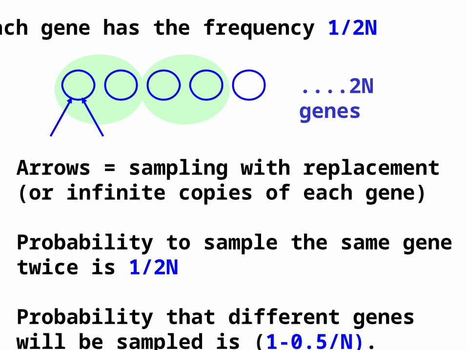
Gene poolA population with N zygotes has 2N genes in the gene pool
....2N
Gene pool means all genes in a population. It is convenient to consider genes at one locus. The gene pool is independent on how (or if) a population is organised in zygotes.
e.g 2 zygotes with 4 genes in the picture above
....2N genes
Each gene has the frequency 1/2N
Arrows = sampling with replacement (or infinite copies of each gene) Probability to sample the same gene twice is 1/2N Probability that different genes will be sampled is (1-0.5/N).

Genes can be IBD (identical by descent). The probability is the coancestry (f).
f= coancestry

The gene pool is often structured in individuals
The probability that the genes in two specific individuals are IBD is the coancestry between these two individuals.
f = coancestry
Individual A Individual B

F= inbreeding
For self-coancestry, the genes need not to be different. If they are different f=F; if the same f=1; average f=(1+F)/2.
The probability that the two different genes in the same zygote are IBD is the coefficient of inbreeding (F).

Different mechanisms genes sampled from a population may be IBD:
1. The same gene sampled twice (drift);
2. The genes are homologous genes from the same individual (inbreeding),
3. The genes originate from different individuals (relatedness).

Coancestries arranged in a coancestry matrix
Ind 1 2 3
1 0.5 0.25 0
2 0.25 0.5 0
3 0 0 1
The values along the diagonal (self-coancestries) appear only once.
Symmetric, thus f2,1= f1,2
Coefficient of relationship are often arranged in such a matrix, (numerator matrix), in absence of inbreeding these values are double as large.
We denote a certain value by f2,1=0.25

Relative Coancestry (f,)
Unrelated 0
Half sibs 0.125
Full sibs 0.25
Parent-offspring 0.25
Cousin 0.0625
Itself (self-coancestry)
0.5
Coancestries are probabilities, thus 0 f 1.
Examples of coancestry

Group coancestry
mother
sister
aunt
uncle
cousin
What is the average relatedness (group coancestry) of this ”family”?

To get overall probability; average over all individual probabilities, f.Group coancestry equals the average of all N2 coancestry values among all combinations of the N individuals in a population (or the average of all 4N2 combinations of individual genes). We could as well define group coancestry as this average, the advantage of the probabilistic definition appears in more complex situations.
f
Group coancestry
Let's put all homologous genes in a big pool and select two (at random with replacement). The probability that two are IBD we define as group coancestry. (, this term was introduced by Cockerham 1967).

Ind 1 2 3
1 0.5 0.25 0
2 0.25 0.5 0
3 0 0 1
Sum of the 9 values in matrix= 2.5; Average = group coancestry = 2.5/9 = 0.278
Note that self-coancestries appear once, while other coancestries appear twice (reciprocals).

If all individuals in a population are related in the same pattern, it is enough to calculate the N coancestries for a single individual. Self-coancestry is the group coancestry for a population with a single member. All members in a full sib family have equal coancestries to all other individuals. Thus it is enough to construct the coancestry matrix for full sib families (and make some thinking). Group coancestry depends on relatedness, not how uniting gametes are arranged. A brother is equally related to his brother as to his sister, in spite of that his gametes are able to unite only with those of his sister.

Group coancestry for families
Half sibs
Full sibs
Self sibs
Family size = n, no inbreeding
n
n
8
3
n
n
4
1
n
n
4
12

Group Coancestry may be expressed
2
1 1
N
N
i
N
jij

The term pair-coancestry is used here for the average of all coancestry-values among different individuals excepting self-coancestry. Using “Coancestry” for “pair-coancestry” invites to misunderstandings.
Group-coancestry can be separated in two types: Self-coancestry and pair-coancestry.
The term pair-coancestry (or avearage pair coancestry) is my own construct, I am not sure it is best or has not been better coined by someone else. I have used cross-coancestry earlier and Ola used pair-wise-coancestry, but I did not see what ”wise” was good for.
Pair-coancestry and Self-coancestry

Ind 1 2 3
1 0.5 0.25 0
2 0.25 0.5 0
3 0 0 1
Pair-coancestry for this matrix is 2*0.25/6=0.083
22
1
n
1
3
25.025.015.05.0
n
n
i ijij
n
iii
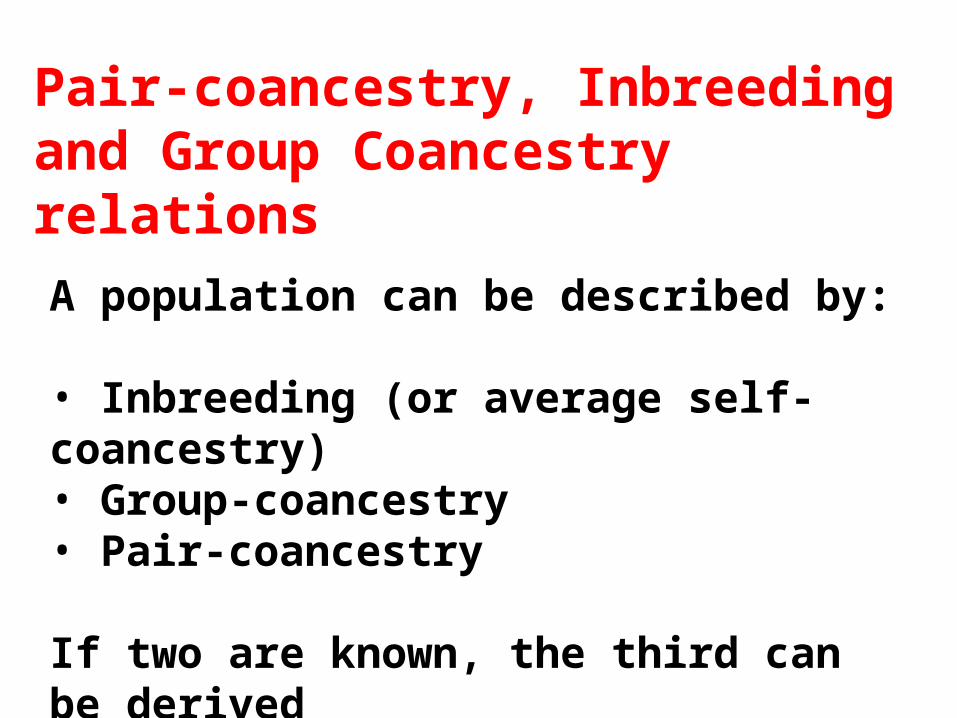
A population can be described by:
• Inbreeding (or average self-coancestry)• Group-coancestry• Pair-coancestry
If two are known, the third can be derived
Pair-coancestry, Inbreeding and Group Coancestry relations

N
fNF
2
)22(1
1
)1(5.0
N
FNf
Using the following relationships, group coancestry and average pair-coancestry can be derived
where: = group coancestry; N = individuals; f = average pair-coancestry; F = average inbreeding.

Linking generations Group coancestry changes at generation shifts can be calculated retrospectively from a known pedigree linking to the founders. Future group coancestry can be calculated with knowledge or assumptions about future pedigrees. For other cases predictions may be made, but this is often far from trivial. Note that there may be doubt if assumptions are realistic (neutral selection, many genes with infinitesimal action etc.)

The link between generations is the gametes.
The gene pool of the offspring is identical to the gene pool of the successful gametes of the parents.
offspring
parents

Consider a pair of genes, which may equivalently be regarded as in offspring zygotes or in parental successful gametes!
A pair of genes in offspring may be IBD as they are copies of the same gene in the parent population. This may happen if a parent has more than one offspring.
2Noffspring offspring
2Nparents parents
2Noffspring offspring

A pair of genes may originate from homogenous genes of the same parental zygote in the parental generation, if that was inbred, the considered genes may be IBD.
F
2Nparents parents
2Noffspring offspring
Different gametes from a parent get coancestry (1+Fparent)/2
Sibs sharing that parent (half sib) get coancestry (1+Fparent)/8.
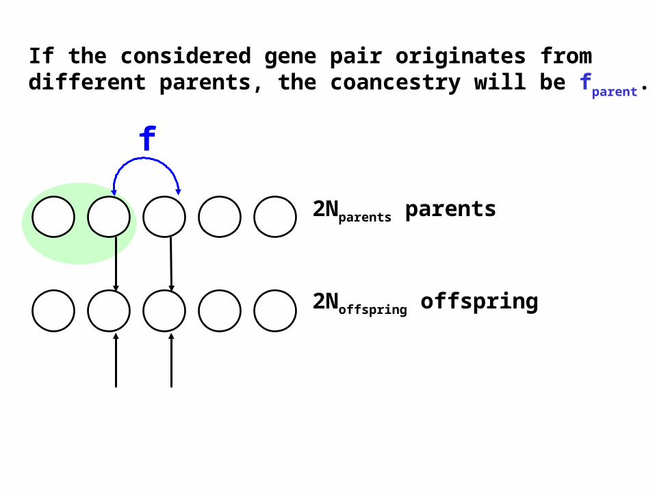
If the considered gene pair originates from different parents, the coancestry will be fparent.
f
2Nparents parents
2Noffspring offspring

IBD may occur by the following mechanisms:
1. The same gene in the current generation is sampled twice,
2. The genes are copies of the same gene in the parental generation,
3. The genes origin from homologous genes in the same inbred parent,
4. The genes come from different, but related, parents.

Gene diversity!

• Evidently 1 - group coancestry is the probability that the genes are non-identical, thus diverse.
Group coancestry and gene diversity
• Group coancestry is the probability that two genes are IBD;
• Diversity means that things are different; • Gene Diversity means that genes are different.

GD = 1 - group coancestry is the probability that the genes are non-identical, thus diverse.
1GD
GD is Gene Diversity!
Group coancestry is a measure of gene diversity lost!
That seems to be something worth knowing!

This way of thinking sees all genes in the source (reference) populations as unique (“tagged”).
GD is similar to expected average heterozygosity (the chance that two genes are different).
Group coancestry based measures are (like inbreeding) relative to some reference population. For forest tree breeding the wild forest usually constitutes a good reference. The gene diversity of the wild forest is 1, and the group coancestry is the share of the initial gene diversity lost.
Monitor group coancestry in tree improvement operations! That says how much gene diversity has been lost since the initiation of the breeding program!

Deriving coancestry and group coancestry
An algorithm for calculation of coancestry and group coancestry (example from Lindgren et al 1997).

Ind
Parent A
Parent B
1 .
.
2 .
.
3 .
.
4 .
.
5 1
1
6 2
3
7 2
3
8 3
4
9 .
.
10+ 5
6
11+ 7
8
12+ 8
9
13+ 9
.
Tabulate pedigree for the population, points (.) for founders. Parents always defined before used as parents.Task: Calculate group coancestry of reds!
4
9
13
8
12
11
10
321
6 75
1,2,3,4,9 and one parent to 13 can be considered founders.

Calculation of the coancestry matrix.
Pedigree for population in the example.Fill the matrix (thus the coancestry of all pair of the 13 individuals) using the pedigree information.This can be done step by step. Fill rows from left to right Start with the diagonal element Proceed leftwards to the row’s end
Ind
1
2
3
4
5
6
7
8
9
10+
11+
12+
13+
1
0.5
0
0
0
0.5
Ind
Parent A
Parent B
1
.
.
2
.
.
3
.
.
4
.
.
5
1
1

Ind
1
2
3
4
5
6
7
8
9
10+
11+
12+
13+
1
0.5
0
0
0
0.5
0
0
0
0
0.25
0
0
0
2
0
0.5
As the matrix is symmetric, column values can be filled from the row
Start with next diagonal

Ind
1
2
3
4
5
6
7
8
9
10+
11+
12+
13+
1
0.5
0
0
0
0.5
0
0
0
0
0.25
0
0
0
2
0
0.5
0
0
0
0.25
0.25
0
0
0.125
0.125
0
0
3
0
0 0.5
0
0
0.25
0.25
0.25
0
0.125
0.25
0.125
0
4
0
0
0
0.5
0
0
0
0.25
0
0
0.125
0.125
0
5
0.5
0
0
0
0.75
0
0
0
0
0.375
0
0
0
6 0
0.25
0.25
0
0
0.5
The matrix below has been filled to element (6,6). Individual 6 has parents 2 and 3, it is demonstrated how diagonal element (6,6) is filled.
The diagonal (6,6)=0.5+(3,2)=0.5+0Self-coancestry = (1+F)/2 = average of 0.5 and coancestry for parents 2 and 3.
Ind
Parent A
Parent B
1
.
.
2 .
.
3 .
.
4 .
.
5 1
1
6 2
3

Ind
1
2
3
4
5
6
7
8
9
10+
11+
12+
13+
1
0.5
0
0
0
0.5
0
0
0
0
0.25
0
0
0
2
0
0.5
0
0
0
0.25
0.25
0
0
0.125
0.125
0
0
3
0
0 0.5
0
0
0.25
0.25
0.25
0
0.125
0.25
0.125
0
4
0
0
0
0.5
0
0
0
0.25
0
0
0.125
0.125
0
5
0.5
0
0
0
0.75
0
0
0
0
0.375
0
0
0
6 0
0.25
0.25
0
0
0.5
The matrix below has been filled to element (6,7). Individual 8 has parents 3 and 4, it is demonstrated how off-diagonal element (6,8) is filled.
0.25
0.125
The off diagonalthe average of coancestry with 6 and the parents to eight (3 and 4) (6,8)=0.5[(6,3)+(6,4)]=0.5[0.25+0]=0.125The average of the parents to 7’s coancestry with 6.
3
.
.
4
.
.
5
1
1
6
2
3
7
2
3
8
3
4
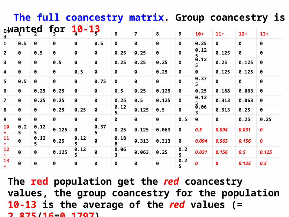
The full coancestry matrix. Group coancestry is wanted for 10-13
Ind 1
2
3
4
5
6
7
8
9
10+
11+
12+
13+
1
0.5
0
0
0
0.5
0
0
0
0
0.25
0
0
0
2
0
0.5
0
0
0
0.25
0.25
0
0
0.125
0.125
0
0
3
0
0
0.5
0
0
0.25
0.25
0.25
0
0.125
0.25
0.125
0
4
0
0
0
0.5
0
0
0
0.25
0
0
0.125
0.125
0
5
0.5
0
0
0
0.75
0
0
0
0
0.375
0
0
0
6
0
0.25
0.25
0
0
0.5
0.25
0.125
0
0.25
0.188
0.063
0
7
0
0.25
0.25
0
0
0.25
0.5
0.125
0
0.125
0.313
0.063
0
8
0
0
0.25
0.25
0
0.125
0.125
0.5
0
0.063
0.313
0.25
0
9
0
0
0
0
0
0
0
0
0.5
0
0
0.25
0.25
10+
0.25
0.125
0.125
0
0.375
0.25
0.125
0.063
0
0.5
0.094
0.031
0
11+
0
0.125
0.25
0.125
0
0.188
0.313
0.313
0
0.094
0.563
0.156
0
12+
0
0
0.125
0.125
0
0.063
0.063
0.25
0.25
0.031
0.156
0.5
0.125
13+
0
0
0
0
0
0
0
0
0.25
0
0
0.125
0.5
The red population get the red coancestry values, the group coancestry for the population 10-13 is the average of the red values (= 2.875/16=0.1797).

Status number • Status number is half the inverse of
group coancestry
2
1SN

Or, equivalently
• Status number is half the inverse of the probability that two genes drawn at random are IBD.
2
1SN

An attractive property of the status number is that it is the same as the census number for a population of unrelated, non-inbred trees.
Status Number
Status number is an effective number. It relates a real population to an ideal population. The ideal population consists of unrelated, non-inbred trees with the same probability of IBD.
Status number is an intuitively appealing way of presenting group coancestry, as it connects to the familiar concept of number (population size).
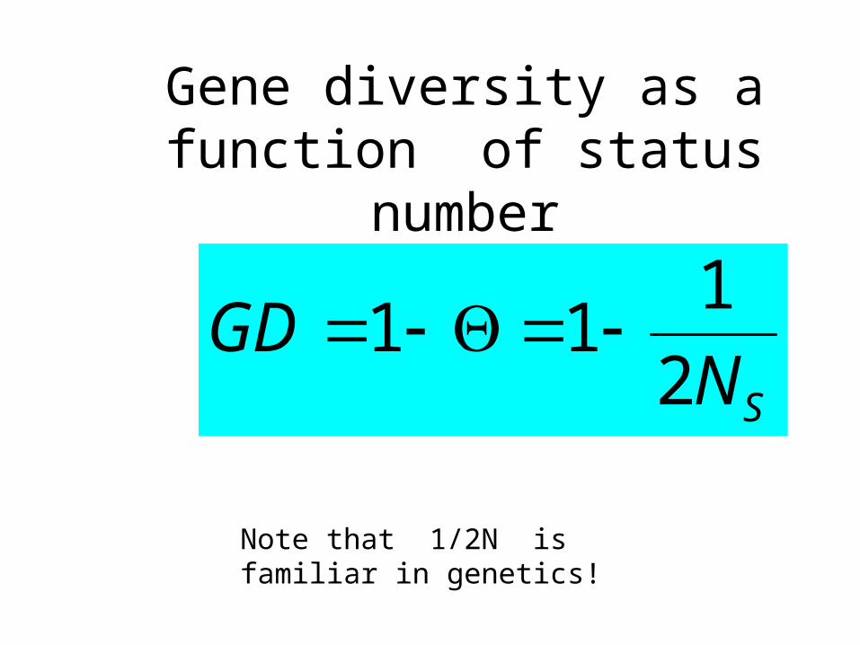
SNGD
2
111
Gene diversity as a function of status number
Note that 1/2N is familiar in genetics!

The status number says that the probability to draw two genes IBD is the same as if it were so many unrelated non-inbred individuals contributing to the gene pool. Therefore we can call it an effective number.
The ratio of the status number and the census number is useful, thus Nr=Ns/N. I call this the relative status number.

An example of the predicted drop of status number over time in a breeding program POPSIM simulation; BP=100; four controlled matings made for each member of the breeding population, the family size was 40, the next generation was recruited from the previous by phenotypic selection, the initial heritability was 0.2.
(Lindgren et al 1997).

The drop of Gene DiversityThe same data looks less drastic when considering gene diversity!This is to exemplify what may happen to Gene Diversity during breeding (from Lindgren et al 1997). Data from a simulated breeding program. POPSIM simulation; Breeding Population=100; four controlled matings made for each member of the breeding population, the family size was 40, the next generation was recruited from the previous by phenotypic selection (selecting the best 100 among the offspring considering only the phenotype), the initial heritability was 0.2.

0
5
10
15
20
25
30
35
40
45
50
1 2 3 4 5 6 7 8 9 10
Generation
Sta
tus
num
ber
From Lindgren et al 1996, Silvae Genetica
Breeding population size 50, differently managed over generations
Mating Offspring/parentSelfing 2 (1=2) Full sibbing 2random 2random random

Some properties of status number
• NS can never be higher than the census number (N);
NS can never be lower than 0.5 (NS of a gamete);
NS considers relatedness and inbreeding;
NS may be derived for any hypothetical population (with known relatedness
patterns to a known source population). It is irrelevant if "population members" belong to the same generation or the same “subpopulation”; NS cannot exceed the minimum N in any of the preceding generations, if all
ancestors are confined to a range of discrete generations; NS does not care about the gender of the population members;
NS after a generation shift depends only on the number of offspring for each
parent; NS is independent on the mating patterns of the parents it is derived from;
NS describes a gene pool, not how it is organised;
NS usually declines at generation shifts, but it can rise if the initial genomes
may get a more equal representation after a generation shift than before. Mating patterns matters for development of NS in later generations, and they are constraining for
possible values of NS, thus they are a relevant matter, even if not formally.
NS is closely associated to inbreeding, but the associations become cleared with the concept group
coancestry, they are better developed in connection to that concept.

Status number and group coancestry measure gene dispersion!
Cockerham (1969) concluded that the variance of the gene frequency (that’s the mean of the occurrence of a gene) is
p
p p2 1 ( )
this can equivalently be expressed
p
p pN s
2 12
( )
This is the binomial expression of the variance for the gene frequency in a population with Ns non-
inbred non-related members!

Status number is the size of unrelated non inbred trees sampled from the reference population, which have the same drift as the accumulated drift of the population under study (compared to the reference population).
Gene frequency
Generations
Gene frequency over generations
Status number

Effective number An effective number (size) is an effort to characterise a complicated system by the number of individuals in a simpler and more ideal system, which have the same characteristic value or behaviour from some important respect. Effective population size in the inbreeding or variance sense To understand how these concepts are usually used in genetics one has to understand that they compare population dynamics to that of an "ideal population". (Caballero, 1994 p 658 from Fisher 1930) “An idealized population consists of infinite, randomly mated base populations subdivided into infinitely many subpopulations, each with a constant number, N, of breeding individuals per generation. In each subpopulation, parents produce an infinite number of male and female gametes into a large pool from which only 2N are sampled and united to produce the N zygotes of the following generation...Both the sampling of the gametes and their union (including self-fertilization) are random, so that all parents have an equal chance of producing offspring.... Generations do not overlap.”(there are some less important omissions)

Based on this “The effective size of a population is defined as the size of an idealized population which would give rise to the variance of change in gene frequency or the rate of inbreeding observed in the actual population under consideration”
Thus, effective population size says how a studied population develops over generations compared to the development of the ideal population. Note that the number is not associated to any particular generation.

Usually two variants of effective population sizes are recognised, the inbreeding sense and the variance sense (there are more).
The classical effective population size is the size of an ideal population, which accumulates inbreeding or widen variance at the same rate as the ideal population. The status number does not do that. The status number measures a state, the classical effective population size measure a rate.

The status number and the "traditional" effective population size are sometimes similar when studied after respectively over the first generation turn over, in particular when large progenies are considered. An analogy: Distance and a speed may appear the same, if studied over a unit time from a common starting point.
E.g. many results concerning diversity from Lindgren and Wei (e.g. Wei 1995) and others can be considered as status number results even if different variants of effective numbers or diversity has been used. But then families are limited there is no equivalence.

Currently I believe effective population size in the inbreeding sense is a concept we have better to forget about in forest tree improvement, it is much better just to try to predict the inbreeding than stray around in never needed - but complex - calculations of an abstract and often misleading entity.
I have easier to see the need and accept some intuitively odd characteristics for the effective population size in the variance sense, there may be a need for such calculations, and status number may be viewed as a complement.

Status number, group coancestry and variance effective number
These concepts may (in an over-simplified world) be linked
Where NS = status number, NV variance effective number and t
generations Can also be expressed:
))/5.01(1/(5.0 tVS NN
tNN
NV
V
S /lim
))/5.01(1( tVt N

Gene frequency
Generations
Gene frequency over generationsVariance effective numberStatus number
The initial founders matters, so the formulas are more relevant for the development over generations that the absolute values.

Different effective numbers for the same object It may be of interest to see how different effective numbers compare for the same object, this has been done by Kjaer and Wellendorf (1998) for a Norway spruce seed orchard and its crop:
Entity Value
Number of clones in seed orchard 100
Variance effective population size 236.7
Inbreeding effective population size 18.1
Status number of the crop 70.4
Note that the effective population size expresses changes between the 100 parental clones and their progeny, while the status number expresses the relationship between the orchard seeds and the base population with unrelated non inbred trees (the “wild forest”) the seed orchard clones were drawn from.

Status number is the number of clones drawn from the wild forest which has the same group coancestry and gene diversity as the seeds harvested in the orchard. Inbreeding interpretationStatus number is the number of clones drawn from the wild forest which following random mating would produce as much inbreeding as expected in the seed crop of the forest created with the seed orchard crop. Drift interpretationStatus number is the number of clones drawn from the wild forest, which has the same expected drift in gene frequencies as the seeds harvested in the orchard. Note that the variance effective population size is a measure of the drift between the seed orchard and its seed,
Status number may be interpreted
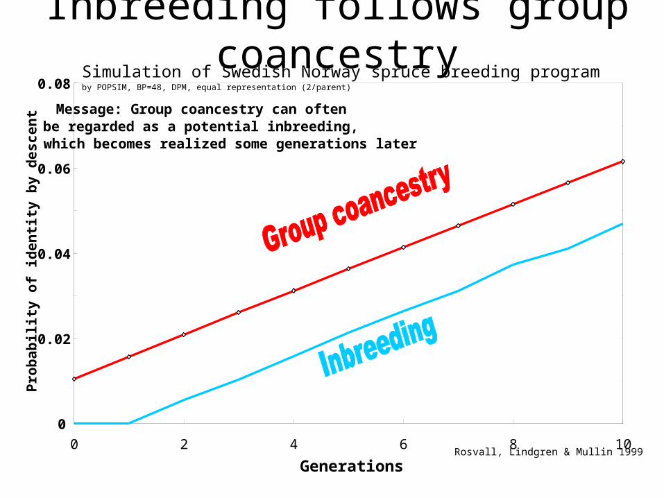
Inbreeding follows group coancestrySimulation of Swedish Norway spruce breeding program by POPSIM, BP=48, DPM,
equal representation (2/parent)
0
0.02
0.04
0.06
0.08
0 2 4 6 8 10
Generations
Pro
ba
bil
ity
of
ide
nti
ty b
y d
es
ce
nt
f
Rosvall, Lindgren & Mullin 1999
Message: Group coancestry can often be regarded as a potential inbreeding, which becomes realized some generations later

What is called FIS is the difference between inbreeding and
cross-coancestry. If Hardy-Weinberg balance they are equal (the same chance of IBD if the genes are in the same as in different individuals).
I have developed the relations with as follows:
NF
NFFFIS /)1(5.01
/)1(5.0
Group coancestry and Wright's F-statistics

Forest tree breeding and status number
• are still very close to the founders
• thus close to the "wild forest“, a natural reference point for evaluating impact of breeding
• deal with few generations
• change strategy between generations
• structure population in sublines
• "own" and control the breeding population
The status number concept is more useful to forest tree breeders than other breeders or geneticists. Forest tree breeders :