1

Dr. James Brown

Quantitative evaluation of probabilistic prediction systems

with observations

HYACINTS seminar: 09/10/09

james.d.brown@noaa.gov

Hydrologic Ensemble Prediction Group, NOAA/NWS

2

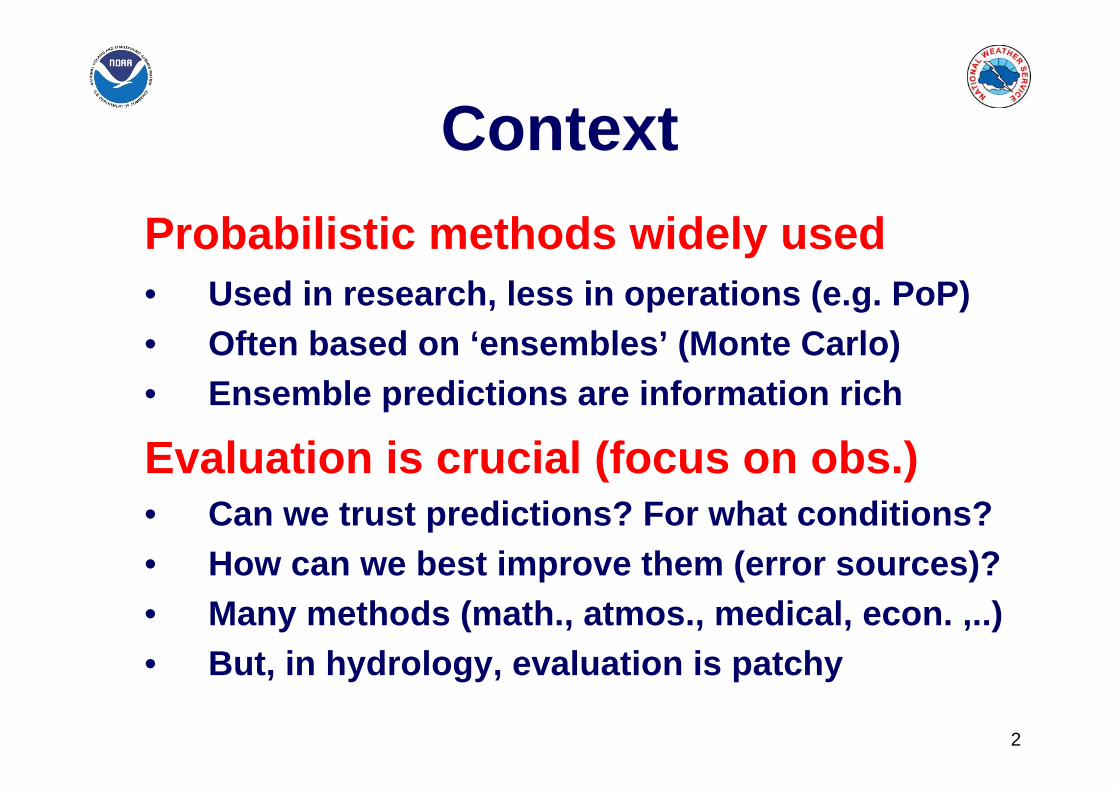
Probabilistic methods widely used• Used in research, less in operations (e.g. PoP)• Often based on ‘ensembles’ (Monte Carlo)• Ensemble predictions are information rich

Evaluation is crucial (focus on obs.)• Can we trust predictions? For what conditions?• How can we best improve them (error sources)?• Many methods (math., atmos., medical, econ. ,..)• But, in hydrology, evaluation is patchy

Context

3

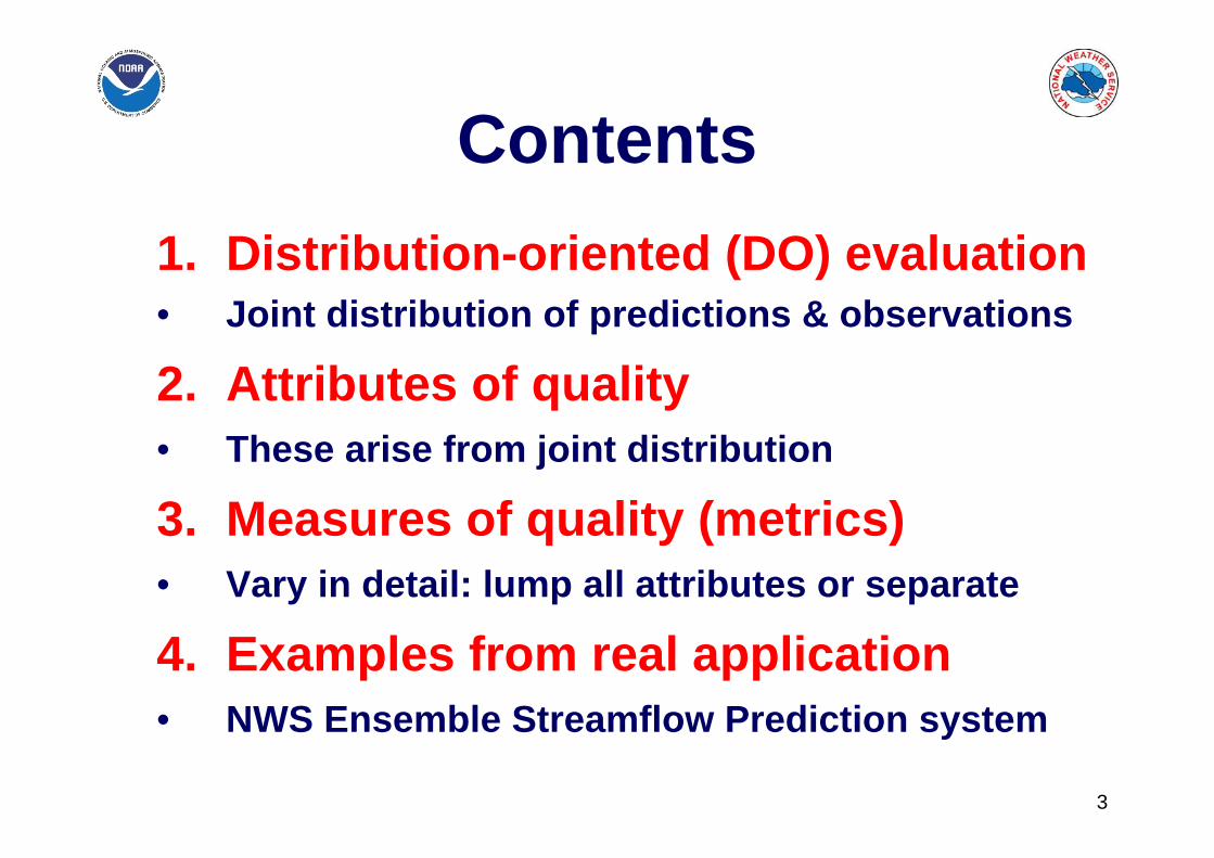
1. Distribution-oriented (DO) evaluation • Joint distribution of predictions & observations

2. Attributes of quality • These arise from joint distribution

3. Measures of quality (metrics)• Vary in detail: lump all attributes or separate

4. Examples from real application• NWS Ensemble Streamflow Prediction system

Contents

4

1. Distribution-oriented approaches

5

Predictions and observations• Q, cont. (e.g. flow). We forecast and observe. • Consider a discrete event (e.g. flood): {Q > qv}. • Prob. prediction (y) and observation (x).

How good is our model for {Q>qv}?• Two ways to look at joint distribution:• “calibration-refinement”• “likelihood-base-rate”

DO evaluation

n1,..., i 0} else ,q Q if {1 x],qPr[Qy vivi =>=>=

b(y)y)|a(xy)f(x, ⋅=d(x)x)|c(yy)f(x, ⋅=

6

What does f(x,y) represent?• Is Q variable in space and time? What support?• What about forecast lead-time?

Can we estimate its properties?• Pairs: time and/or space substitutes as repetition• …if max. daily flow, 1-day ahead, at Station A…• …over 1 year:• In this case, pool data in time• Try to avoid model calibration period (split?)

Considerations

]}y,[x],...,y,{[x 36536511

7

2. (Some) quality attributes

8

Calibration-refinement: a(x|y)·b(y)• Reliable if (e.g.):• “When , should observe 20% of time”• Sharp if:• Aim: “maximize sharpness subject to reliability”

Likelihood-base-rate: c(y|x)·d(x)• Discriminatory if (e.g.):

• “Forecasts easily separate flood from no flood”

(Some) attributes of quality

p pp]y|E[x ∀==

1 or 0y →0.2y =

0]x|E[y1]x|E[y =>>=

9

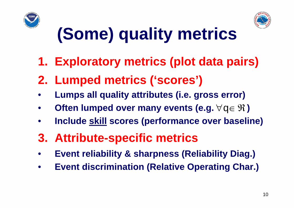
3. (Some) quality metrics

10

1. Exploratory metrics (plot data pairs)2. Lumped metrics (‘scores’)• Lumps all quality attributes (i.e. gross error)• Often lumped over many events (e.g. )• Include skill scores (performance over baseline)

3. Attribute-specific metrics• Event reliability & sharpness (Reliability Diag.)• Event discrimination (Relative Operating Char.)

(Some) quality metrics

∀ ∈q ℜ

11

Highest member

90 percent.80 percent.

50 percent.

20 percent.10 percent.

‘Error’ for 1 forecast

Lowest member

Zero error line

Observed precipitation [mm]

A ‘conditional bias’, i.e. a bias that depends uponthe observed precipitation value.

0 10 20 30 40 50 60 70 80

EPP precipitation ensembles (1 day ahead total)

Erro

r (en

sem

ble

mem

ber -

obse

rved

) [m

m]

Precipitation is bounded at 0

Exploratory metric: box plots5

4

3

2

1

0

-1

-2

-3

-4

-5

“Blown forecasts”

12

0.0 10 20 30 40 50 60

Cum

ulat

ive

prob

abili

ty

Flow (Q) [cms]

1.0

0.8

0.6

0.4

0.2

0.0

Forecast: FY(q)=Pr[Y ≤q]

Observed: FX(q)=Pr[X≤q]

• Then average acrossmultiple forecasts

• Small scores = better• Note quadratic form:- can decompose- extremes count less

Lumped metric: Mean CRPS

dq(q)}F(q){FCRPS 2XY∫

∞

∞−

−=

13

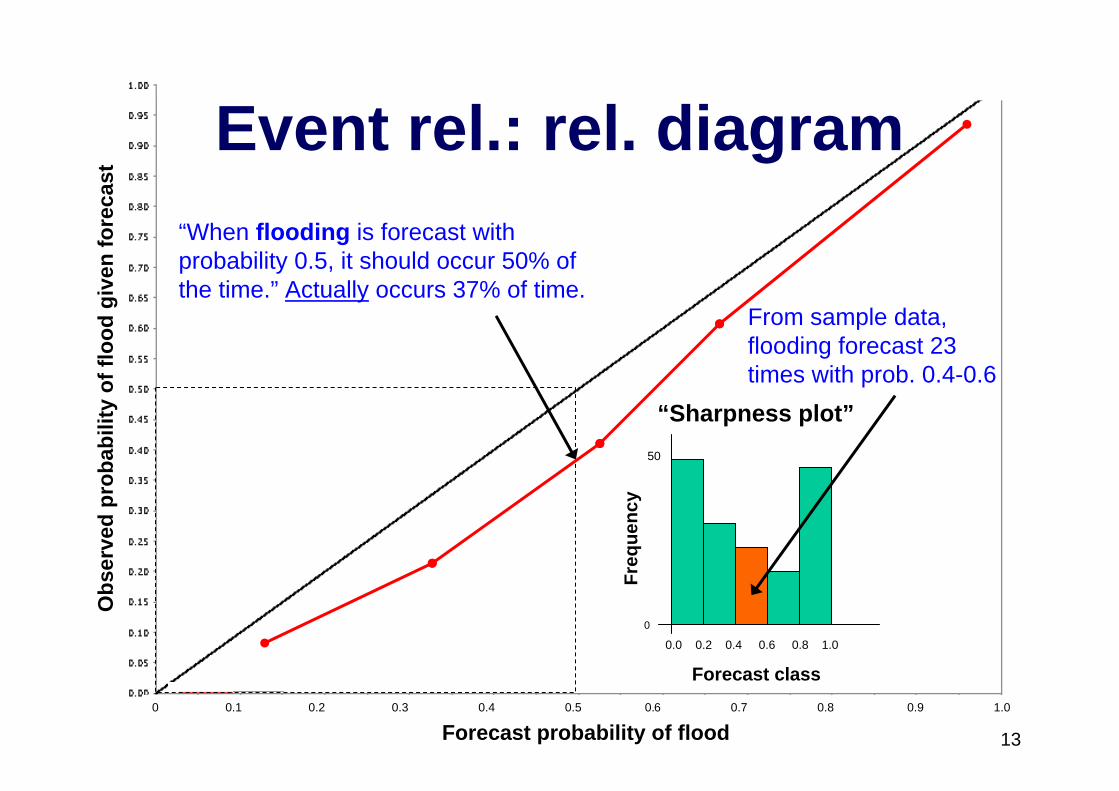
Event rel.: rel. diagramO

bser

ved

prob

abili

ty o

f flo

od g

iven

fore

cast

“Sharpness plot”

0 0.1 0.2 0.3 0.4 0.5 0.6 0.7 0.8 0.9 1.0

Forecast probability of flood

“When flooding is forecast withprobability 0.5, it should occur 50% of the time.” Actually occurs 37% of time.

0.0 0.2 0.4 0.6 0.8 1.0

50

0

From sample data, flooding forecast 23 times with prob. 0.4-0.6

Freq

uenc

y

Forecast class

14

Event disc.: ROC (decision)Pr

obab

ility

of D

etec

tion

[TP/

(TP+

FN)]

Probability of False Detection [FP/(FP+TN)]

0.00 1.0

1.0

Climatological prob. forecast“sitting on the fence”

W TP FP

!W FN TN

flood !flood

Warn flood (W) when y>0.1“OK to cry wolf!”

Perfect

Warn flood (W) when y>0.9“Must not cry wolf!”

15

4. Real example

16

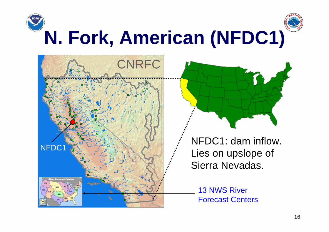
N. Fork, American (NFDC1)

13 NWS River Forecast Centers

CNRFC

NFDC1NFDC1: dam inflow.Lies on upslope of Sierra Nevadas.

17

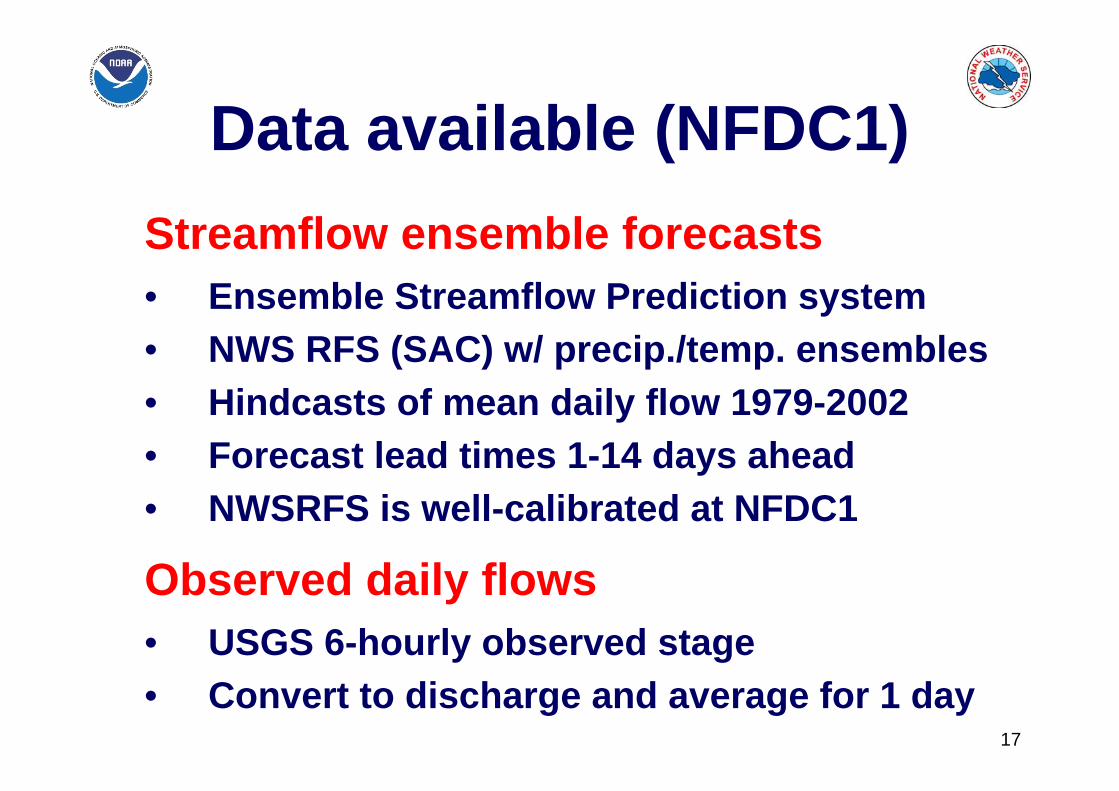
Streamflow ensemble forecasts• Ensemble Streamflow Prediction system• NWS RFS (SAC) w/ precip./temp. ensembles• Hindcasts of mean daily flow 1979-2002• Forecast lead times 1-14 days ahead• NWSRFS is well-calibrated at NFDC1

Observed daily flows• USGS 6-hourly observed stage• Convert to discharge and average for 1 day

Data available (NFDC1)

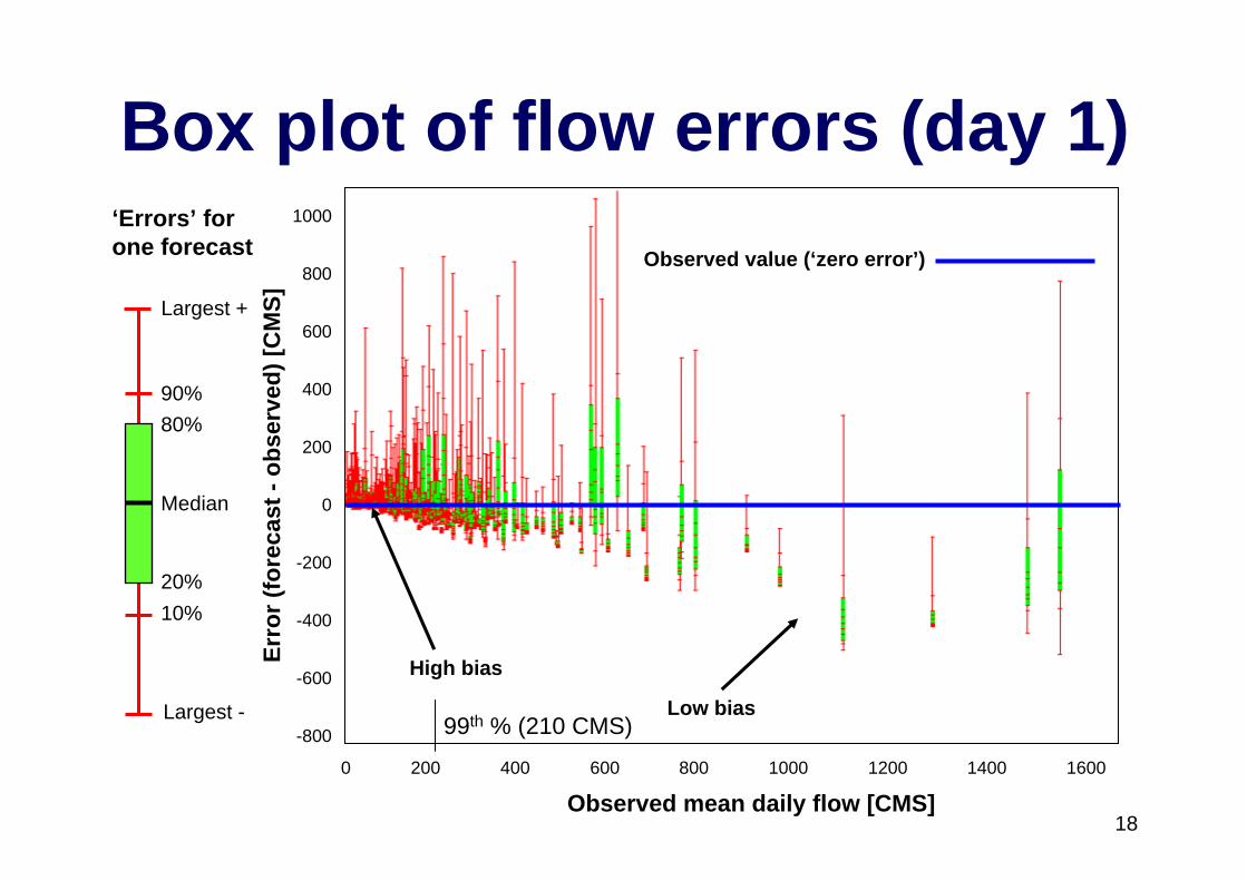
Box plot of flow errors (day 1)

18

Largest +

90%80%

Median

20%10%

‘Errors’ forone forecast

Largest -

Observed value (‘zero error’)

Observed mean daily flow [CMS]

1000

800

600

400

200

0

-200

-400

-600

-800

Erro

r (fo

reca

st -

obse

rved

) [C

MS]

Low bias

High bias

0 200 400 600 800 1000 1200 1400 1600

99th % (210 CMS)

Lumped error statistics

19

Tests ofensemble mean

Lumped error in probability

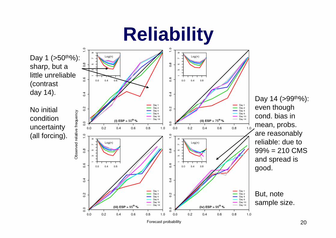
Reliability

20

Day 1 (>50th%):sharp, but a little unreliable(contrast day 14).

No initial conditionuncertainty(all forcing).

Day 14 (>99th%):even thoughcond. bias in mean, probs. are reasonably reliable: due to99% = 210 CMSand spread isgood.

But, note sample size.

ROC

21

Forecast easily beat climatologyrepresented bydiagonal (climatology system: forecast prob.is long-term averagefrequency)

Forcing verygood for large events(orographiclifting = predictable).

22

Public download soon at: http://www.nws.noaa.gov/iao/iao_hydroSoftDoc.php

“Ensemble Verification System”

Literature

23

• Bradley, A. A., Schwartz, S. S. and Hashino, T., 2004: Distributions-Oriented Verification of Ensemble Streamflow Predictions. Journal of Hydrometeorology, 5(3), 532-545.

• Brown, J.D., Demargne, J., Liu, Y. and Seo, D-J (submitted) The Ensemble Verification System (EVS): a software tool for verifying ensemble forecasts of hydrometeorological and hydrologic variables at discrete locations. Submitted to Environmental Modelling and Software. 52pp.

• Gneiting, T., F. Balabdaoui, and Raftery, A. E., 2007: Probabilistic forecasts, calibration and sharpness. Journal of the Royal Statistical Society Series B: Statistical Methodology, 69(2), 243 – 268.

• Hsu, W.-R. and Murphy, A.H., 1986: The attributes diagram: A geometrical framework for assessing the quality of probability forecasts. International Journal of Forecasting, 2, 285-293.

• Jolliffe, I.T. and Stephenson, D.B. (eds), 2003: Forecast Verification: A Practitioner’s Guide in Atmospheric Science. Chichester: John Wiley and Sons, 240pp.

• Mason, S.J. and Graham N.E., 2002: Areas beneath the relative operating characteristics (ROC) and relative operating levels (ROL) curves: Statistical significance and interpretation, Quarterly Journal of the Royal Meteorological Society, 30, 291-303.

• Murphy, A. H. and Winkler, R.L., 1987: A general framework for forecast verification. Monthly Weather Review, 115, 1330-1338.

• Wilks, D.S., 2006: Statistical Methods in the Atmospheric Sciences, 2nd ed. Academic Press, 627pp.