
Quantitative Confocal Microscopy of Dense Colloidal Systems ...
296
Quantitative Confocal Microscopy of Dense Colloidal Systems Matthew Jenkins Thesis submitted for the degree of Doctor of Philosophy School of Physics University of Edinburgh 2005
Transcript of Quantitative Confocal Microscopy of Dense Colloidal Systems ...

Quantitative Confocal Microscopy of DenseColloidal Systems
Matthew Jenkins
Thesis submitted for the degree of Doctor of Philosophy
School of Physics
University of Edinburgh
2005


Abstract
This document describes an experimental investigation into dense collections of hardspherical particles just large enough to be studied using a light microscope. These parti-cles display colloidal properties, but also some similarities with granular materials. Weimprove the quantitative analysis of confocal micrographs of dense colloidal systems,which allows us to show that methods from simulations of granular materials are use-ful (but not sufficient) in analysing colloidal systems, in particular colloidal glasses andsediments.
Collections of spheres are fascinating in their own right, but also make convincing modelsfor real systems. Colloidal systems undergo an entropy-driven fluid-solid transition for hardspheres and a liquid-gas transition for suitable inter-particle attraction. Furthermore, experi-mental colloidal systems display a so far not well-understood glass transition at high densi-ties, so that the equilibrium state is not achieved. This may be due to limited experimentaltimescales, but experiments under reduced gravity (both using the Space Shuttle and density-matching solvents) suggest that it is not.
Most colloidal studies have used scattering (i.e. non-microscopical) techniques, which pro-vide no local information. Microscopy (particularly confocal) allows individual particles andtheir motion to be followed. However, quantitative microscopy of densely-packed, solidly-fluorescent particles, such as colloidal glasses, is challenging. We report, to our knowledge forthe first time, a quantitative measure of confidence in individual particle locations and use thismeasure in an iterative best-fit procedure. This method was crucial for the investigation of thecolloidal samples reported in this thesis.
One of the disadvantages of microscopy is that it requires particles too large to be truly col-loidal; gravity is no longer negligible. The particles used here rapidly sediment to form solid”plugs”, which are supposedly ”random close packed” (RCP). At least in some cases, this isnot the case, since some particles remain free to move. This observation, as well as some liter-ature results, suggest that gravity has some influence on the structure of the sediment. In thisdocument we consider some ideas from literature not normally considered in colloidal studies.Firstly, we discuss the RCP state, and the preferred Maximally Random Jammed state. Sec-ondly, we borrow a technique designed to identify structures known as bridges in simulationsof granular materials.
Finding bridges, i.e. structures stable against gravity, in colloidal samples is the primary aim ofthis thesis. Gravity is important in colloidal sphere packings both in sediments and in glasses;its effect is not known but the best available candidate is bridging. The basic results of thisanalysis, the bridge size distributions, are close to those for granular systems, but differ littlefor samples of different volume fractions. We identify important stages of the analysis whichrequire more investigation. Whilst questioning the usefulness of the bridge properties, we iden-tify some related packing properties which show interesting trends. No theoretical predictionsexist for these quantities. We investigated initially a non-density-matched system, but compareour results with a nearly density-matched system. The results from both systems are similar,despite the particles apparently acquiring a charge in the latter case.
This thesis shows that reliable confocal microscopy of very dense systems of solidly-fluorescentparticles is possible, and provides a range of unreported properties of dense sedimenting andsedimented nearly-Brownian sphere packings. It provides several suggestions for further anal-ysis of these experimental systems, as well as some to be performed by those who simulategranular matter.


Declaration
The experiments, analysis and interpretation described in this work have been my own, incollaboration with my colleagues.
I declare that I composed entirely this thesis, and that it has not been submitted in any previousapplication for a degree.
Matthew JenkinsDecember 2005


Acknowledgements
There are a number of people who were very helpful to me while I undertook this thesis.
Firstly, my now main supervisor Stefan, who is famously optimistic and never objects to ex-plaining the most trivial things.
My second supervisor Mark Haw doesn’t miss much, and always has good ideas for things Icould try. He has also commented very carefully and diplomatically on a number of things Ihave written.
I would like to thank Mike Cates for a consistent interest in my work, as well as keeping acareful eye on my project.
If it weren’t for Wilson Poon, I would never have started in Soft Matter, and I am grateful thathe accepted me back to undertake this PhD.
Gary Barker at the Institute for Food Research in Norwich was responsible for the bridginganalysis in the first place. He has been very helpful, both in his comments and by providingraw data and sample analysis.
This work was done in conjunction with Rhodia. I would like to thank all of those involvedwith this project for showing me the interesting work and facilities at Aubervilliers, as well asfor providing the motivation for this project. Most importantly, thanks to Steve Meeker for hisinterest and involvement in the project, and a few good beers.
It goes without saying that any Edinburgh Soft Matter thesis requires acknowledgement ofAndy Schofield, not just for experimentalists (for the particles, of course), but for everyoneelse for their inevitably more interesting social lives.
For technical advice, Jochen Arlt and the users of COSMIC have been very helpful. For con-focal and IDL support, particularly at first, I acknowledge Paul Smith. I should also mentionEric Weeks, who very kindly made the particle location code available to us in the first place.
I would like to mention all my friends from the list of past and present members of the Physicsdepartment, not least those on the squash ladder, for their consistent interest in and support ofmy work.
Most importantly, of course, are my parents, my brother, and Alice. Thank you very much foryour continued support.


Contents
1 Introduction 1
1.1 Sphere Packings are Interesting . . . . . . . . . . . . . . . . . . . . . . . . . . 1
1.1.1 Colloidal Systems . . . . . . . . . . . . . . . . . . . . . . . . . . . . 3
1.1.2 Granular Systems . . . . . . . . . . . . . . . . . . . . . . . . . . . . . 6
1.2 “Nearly Thermal” Systems . . . . . . . . . . . . . . . . . . . . . . . . . . . . 7
1.3 Thesis Layout . . . . . . . . . . . . . . . . . . . . . . . . . . . . . . . . . . . 8
2 Hard Spheres 11
2.1 Packings . . . . . . . . . . . . . . . . . . . . . . . . . . . . . . . . . . . . . . 11
2.1.1 Packing Fraction . . . . . . . . . . . . . . . . . . . . . . . . . . . . . 12
2.1.2 Important Packings . . . . . . . . . . . . . . . . . . . . . . . . . . . . 13
2.1.3 Radial Distribution Function, g(r) . . . . . . . . . . . . . . . . . . . . 15
2.1.4 Volume per Particle: Voronoı Construction . . . . . . . . . . . . . . . 17
2.1.5 Other structural descriptors . . . . . . . . . . . . . . . . . . . . . . . . 18
2.1.6 Is Random Close Packing Well Defined? . . . . . . . . . . . . . . . . 19
2.2 Thermal Systems . . . . . . . . . . . . . . . . . . . . . . . . . . . . . . . . . 22
2.2.1 Phase behaviour of ideal hard sphere systems . . . . . . . . . . . . . . 22
2.2.2 Hard sphere model systems . . . . . . . . . . . . . . . . . . . . . . . 25
2.2.3 Limitations of colloidal systems . . . . . . . . . . . . . . . . . . . . . 29
2.2.4 Evidence for nearly-hard-sphere behaviour in colloidal systems . . . . 30
2.3 Athermal Systems . . . . . . . . . . . . . . . . . . . . . . . . . . . . . . . . . 32
2.3.1 Granulars: a very brief introduction . . . . . . . . . . . . . . . . . . . 33
2.3.2 Geometry and Packings Relevant to Granular Systems . . . . . . . . . 34
2.3.3 Bridges . . . . . . . . . . . . . . . . . . . . . . . . . . . . . . . . . . 37
2.4 Intermediate Systems . . . . . . . . . . . . . . . . . . . . . . . . . . . . . . . 39
2.4.1 Gravitational Peclet Number . . . . . . . . . . . . . . . . . . . . . . . 39
2.4.2 Some intermediate colloidal systems . . . . . . . . . . . . . . . . . . . 40
2.5 Broader Context: A Jamming Phase Diagram? . . . . . . . . . . . . . . . . . . 41
2.6 Summary and Motivation . . . . . . . . . . . . . . . . . . . . . . . . . . . . . 42
ix

3 Confocal Microscopy of Spherical Colloids 43
3.1 Image formation . . . . . . . . . . . . . . . . . . . . . . . . . . . . . . . . . . 43
3.1.1 The Imaging Process . . . . . . . . . . . . . . . . . . . . . . . . . . . 43
3.1.2 Magnification . . . . . . . . . . . . . . . . . . . . . . . . . . . . . . . 45
3.1.3 Aberrations . . . . . . . . . . . . . . . . . . . . . . . . . . . . . . . . 45
3.2 Resolution . . . . . . . . . . . . . . . . . . . . . . . . . . . . . . . . . . . . . 47
3.2.1 Detector Fidelity: Segmentation and Sampling Theory . . . . . . . . . 47
3.2.2 Imaging System Aperture . . . . . . . . . . . . . . . . . . . . . . . . 49
3.2.3 Coherence of Illumination . . . . . . . . . . . . . . . . . . . . . . . . 51
3.2.4 The Microscope . . . . . . . . . . . . . . . . . . . . . . . . . . . . . 52
3.3 Improvement in Resolution Using Point Scanning Microscopes . . . . . . . . . 55
3.4 The Confocal Microscope in Practice . . . . . . . . . . . . . . . . . . . . . . . 57
3.5 A Mathematical Description of the Imaging Process . . . . . . . . . . . . . . 63
3.6 Modelling the Confocal Image of a Spherical Fluorescent Particle . . . . . . . 70
3.6.1 A model of the system PSF . . . . . . . . . . . . . . . . . . . . . . . . 70
3.6.2 A model of the image of a spherical colloidal particle . . . . . . . . . . 71
3.6.3 A comparison of the modelled SSFs with real data . . . . . . . . . . . 73
3.7 Noise in Images . . . . . . . . . . . . . . . . . . . . . . . . . . . . . . . . . . 76
3.7.1 Signal-to-Noise Ratio (SNR) . . . . . . . . . . . . . . . . . . . . . . . 76
3.7.2 Dealing with noise in images . . . . . . . . . . . . . . . . . . . . . . . 78
3.8 Deconvolution of the Point Spread Function . . . . . . . . . . . . . . . . . . . 78
4 Particle Coordinates from the Confocal Microscope 85
4.1 Achieving suitable images . . . . . . . . . . . . . . . . . . . . . . . . . . . . 86
4.1.1 Digital Representation of Detected Light . . . . . . . . . . . . . . . . 86
4.1.2 Pixel pitch and image size . . . . . . . . . . . . . . . . . . . . . . . . 90
4.1.3 A recipe for capturing good quality images . . . . . . . . . . . . . . . 92
4.1.4 Noise . . . . . . . . . . . . . . . . . . . . . . . . . . . . . . . . . . . 94
4.2 Dealing with noise . . . . . . . . . . . . . . . . . . . . . . . . . . . . . . . . 95
4.2.1 Contrast Gradients . . . . . . . . . . . . . . . . . . . . . . . . . . . . 96
4.2.2 Noise . . . . . . . . . . . . . . . . . . . . . . . . . . . . . . . . . . . 97
4.2.3 Performing the Convolutions . . . . . . . . . . . . . . . . . . . . . . . 98
4.3 Strategies for finding particle centres . . . . . . . . . . . . . . . . . . . . . . . 103
4.3.1 Identify Local Brightness Maxima and Refine . . . . . . . . . . . . . . 104

4.3.2 Particle Location by Deconvolution of the SSF . . . . . . . . . . . . . 108
4.3.3 Many Spheres . . . . . . . . . . . . . . . . . . . . . . . . . . . . . . . 109
4.3.4 The Problem . . . . . . . . . . . . . . . . . . . . . . . . . . . . . . . 110
4.4 Tests of Accuracy . . . . . . . . . . . . . . . . . . . . . . . . . . . . . . . . . 111
4.5 Centroiding . . . . . . . . . . . . . . . . . . . . . . . . . . . . . . . . . . . . 115
4.5.1 A brief literature review . . . . . . . . . . . . . . . . . . . . . . . . . 116
4.5.2 Basic technique and parameters . . . . . . . . . . . . . . . . . . . . . 116
4.5.3 Parameter Optimisation . . . . . . . . . . . . . . . . . . . . . . . . . 117
4.5.4 An Appraisal of the Centroiding Technique . . . . . . . . . . . . . . . 122
4.6 Why the Centroid is not the Particle Centre . . . . . . . . . . . . . . . . . . . 123
4.6.1 Illustration of the problem . . . . . . . . . . . . . . . . . . . . . . . . 124
4.7 SSF refinement: Using the SSF to refine particle coordinates . . . . . . . . . . 128
4.7.1 Achieving a satisfactory SSF . . . . . . . . . . . . . . . . . . . . . . . 129
4.7.2 Assessing the accuracy of each particle location . . . . . . . . . . . . . 130
4.7.3 Establishing the chi-square hypersurface . . . . . . . . . . . . . . . . . 131
4.7.4 Finding the chi-square hypersurface minimum . . . . . . . . . . . . . 132
4.7.5 Some examples of the SSF refinement . . . . . . . . . . . . . . . . . . 136
4.7.6 A closer look at fitting . . . . . . . . . . . . . . . . . . . . . . . . . . 138
4.8 A Comparison of Centroiding and SSF Refinement . . . . . . . . . . . . . . . 143
4.9 Tracking . . . . . . . . . . . . . . . . . . . . . . . . . . . . . . . . . . . . . . 145
5 Sample Preparation and Characterisation 147
5.1 System . . . . . . . . . . . . . . . . . . . . . . . . . . . . . . . . . . . . . . . 148
5.2 Sample Preparation . . . . . . . . . . . . . . . . . . . . . . . . . . . . . . . . 151
5.2.1 Washing the Colloid . . . . . . . . . . . . . . . . . . . . . . . . . . . 151
5.2.2 Charge Stabilisation of Density-Matched Samples . . . . . . . . . . . 153
5.2.3 Particle Radius . . . . . . . . . . . . . . . . . . . . . . . . . . . . . . 154
5.2.4 Determining Volume Fraction . . . . . . . . . . . . . . . . . . . . . . 155
5.2.5 Preparing Samples of Known Volume Fraction . . . . . . . . . . . . . 162
5.3 Experimental equipment . . . . . . . . . . . . . . . . . . . . . . . . . . . . . 163
5.3.1 Sample Mountings . . . . . . . . . . . . . . . . . . . . . . . . . . . . 163
5.3.2 Sample Cell 1 . . . . . . . . . . . . . . . . . . . . . . . . . . . . . . . 165
5.3.3 Sample Cell 2 . . . . . . . . . . . . . . . . . . . . . . . . . . . . . . . 168
5.3.4 Oil Immersion . . . . . . . . . . . . . . . . . . . . . . . . . . . . . . 169

6 Bridges 171
6.1 Identifying bridges . . . . . . . . . . . . . . . . . . . . . . . . . . . . . . . . 171
6.1.1 Stability criterion for spherical particles . . . . . . . . . . . . . . . . . 172
6.1.2 Identifying cooperative stabilisations: mutual stabilisations . . . . . . . 174
6.1.3 An algorithm for identifying bridges . . . . . . . . . . . . . . . . . . . 175
6.2 Bridging Basic Results . . . . . . . . . . . . . . . . . . . . . . . . . . . . . . 186
7 Stability and Bridging Results for Pe grav∼1 195
7.1 Introduction . . . . . . . . . . . . . . . . . . . . . . . . . . . . . . . . . . . . 195
7.2 Description of the Samples Used . . . . . . . . . . . . . . . . . . . . . . . . . 195
7.3 Basic Sample Properties . . . . . . . . . . . . . . . . . . . . . . . . . . . . . 197
7.3.1 Comparison of nominal volume fraction with actual volume fraction . . 198
7.3.2 Radial distribution functions . . . . . . . . . . . . . . . . . . . . . . . 199
7.3.3 Relationship between Mean Coordination Number andΦ . . . . . . . . 201
7.3.4 Sample Evolution . . . . . . . . . . . . . . . . . . . . . . . . . . . . . 202
7.4 Stability Results . . . . . . . . . . . . . . . . . . . . . . . . . . . . . . . . . . 208
7.4.1 An interesting observation . . . . . . . . . . . . . . . . . . . . . . . . 209
7.4.2 Stability Properties . . . . . . . . . . . . . . . . . . . . . . . . . . . . 210
7.4.3 Stabilisation properties for stable particles . . . . . . . . . . . . . . . . 215
7.5 Bridge Results . . . . . . . . . . . . . . . . . . . . . . . . . . . . . . . . . . . 220
7.5.1 Bridge Size Distributions . . . . . . . . . . . . . . . . . . . . . . . . . 220
7.6 Testing for Bridges in Other Directions . . . . . . . . . . . . . . . . . . . . . . 222
8 Stability and Bridging Results for Pe grav∼10−3 225
8.1 Introduction . . . . . . . . . . . . . . . . . . . . . . . . . . . . . . . . . . . . 225
8.2 Description of the Samples Used . . . . . . . . . . . . . . . . . . . . . . . . . 225
8.3 Basic Sample Properties . . . . . . . . . . . . . . . . . . . . . . . . . . . . . 226
8.3.1 Comparison of nominal volume fraction with actual volume fraction . . 226
8.3.2 Phase Diagram . . . . . . . . . . . . . . . . . . . . . . . . . . . . . . 227
8.3.3 Radial distribution functions . . . . . . . . . . . . . . . . . . . . . . . 228
8.3.4 Relationship between Mean Coordination Number andΦ . . . . . . . . 230
8.3.5 Sample Evolution . . . . . . . . . . . . . . . . . . . . . . . . . . . . . 231
8.4 Stability Results . . . . . . . . . . . . . . . . . . . . . . . . . . . . . . . . . . 235
8.4.1 Stability Properties . . . . . . . . . . . . . . . . . . . . . . . . . . . . 235
8.4.2 Stabilisation properties for stable particles . . . . . . . . . . . . . . . . 237
8.5 Bridge Results . . . . . . . . . . . . . . . . . . . . . . . . . . . . . . . . . . . 240
8.5.1 Bridge Size Distributions . . . . . . . . . . . . . . . . . . . . . . . . . 240
8.6 A Discussion of Stability and Bridging in Both Systems . . . . . . . . . . . . . 244

9 Future Work 247
9.1 Further ideas for Particle Location via SSF Refinement . . . . . . . . . . . . . 247
9.2 Stability and Bridging Results . . . . . . . . . . . . . . . . . . . . . . . . . . 248
9.2.1 Routine bridge properties . . . . . . . . . . . . . . . . . . . . . . . . . 249
9.2.2 An untested prediction . . . . . . . . . . . . . . . . . . . . . . . . . . 250
9.3 Suggestions for simulations . . . . . . . . . . . . . . . . . . . . . . . . . . . . 251
10 Conclusion 253
10.1 Particle Location . . . . . . . . . . . . . . . . . . . . . . . . . . . . . . . . . 253
10.2 Stability and Bridging . . . . . . . . . . . . . . . . . . . . . . . . . . . . . . . 253
10.2.1 Stability . . . . . . . . . . . . . . . . . . . . . . . . . . . . . . . . . . 254
10.2.2 Bridging . . . . . . . . . . . . . . . . . . . . . . . . . . . . . . . . . 254
10.3 Comparison of Systems of DifferentPegrav . . . . . . . . . . . . . . . . . . . 255
A A closer look at the system PSF 257
A.1 Some remarks on the model of the system PSF . . . . . . . . . . . . . . . . . 257
A.1.1 Convolution of Two One-dimensional Gaussians . . . . . . . . . . . . 258
A.1.2 Convolution of a one-dimensional Gaussian with itself . . . . . . . . . 259
A.1.3 Recovering a Gaussian from its Autoconvolution . . . . . . . . . . . . 259


Chapter 1
Introduction
This document describes an experimental study into samples of micrometer-sized spheres sus-
pended in a solvent. In it, we discuss improvements to the established (published) techniques
of quantitative confocal microscopy of these systems. We also consider general properties of
dense collections (“packings”) of spheres, and use these to argue that ideas from the realm of
granular matter may be appropriate to colloidal systems. To illustrate the relationship between
these apparently very different systems, we begin with a broad discussion of the collections of
spheres and their behaviour under some important forces.
1.1 Sphere Packings are Interesting
We start from the point of view of the simulationist imaging a favourite pastime of the physicist:
billiards. Almost every first year university physics lecture seems to have some topic that is
well approximated by billiard balls; perhaps it is this fact that instills in physicists a lasting
fascination with hard sphere interactions.
Hard spheres have more than just intrinsic interest, however; they have serious cachet. Ever
since Isaac Newton and David Gregory argued over whether a sphere in three dimensions could
have12 contacting (“kissing”) neighbours or13, hard spheres have been fashionable [1]. Sim-
ilarly impressively, in 1611 Kepler famously contended that the cannon-ball (or greengrocer’s
oranges) packing of spheres is the most efficient way of stacking spheres [1]. This “Kepler
conjecture” confounded mathematicians until 1997, when Thomas Hales finally produced a
much celebrated proof [2]. More recently, the importance of hard spheres as physical models
1
2 CHAPTER 1. INTRODUCTION
was reaffirmed by Bernal, who posited them as models of the liquid state [3]. Since then, the
notoriously difficult experiments have been largely replaced by a very large number of compu-
tational studies in both hard discs and hard spheres.
Hard spheres are much more interesting when subject to forces. In simulations, it is easy to
provide each particle with a motivating force. Simulations have shown that, given the right
impetus, hard spheres behave at very low densities as ideal gases (as they should) [4], that
they can display a fluid-solid freezing transition, and that they can serve as models for gran-
ular materials. By addition of suitable inter-particle forces, the behaviour of collections of
spheres becomes much richer, to include the appearance of a liquid-gas transition for suitable
inter-particle attraction, as well as introducing more exotic states such as gels and the recently
fashionable attractive glasses. Only hard spheres are considered in this thesis; there is still
plenty of interest in even these simple systems.
The theme of this thesis concerns two explicit external forces. These are randomly acting
“Brownian” force, which motivates the particles to wander with no particular preferred direc-
tion through the sample, and the force due to gravity, which acts uniaxially downwards. The
hard sphere interactions between the particles are also very important. As the system density
increases, of course these become much more important. As we will see, cooperative sphere–
sphere interactions are crucial in this thesis.
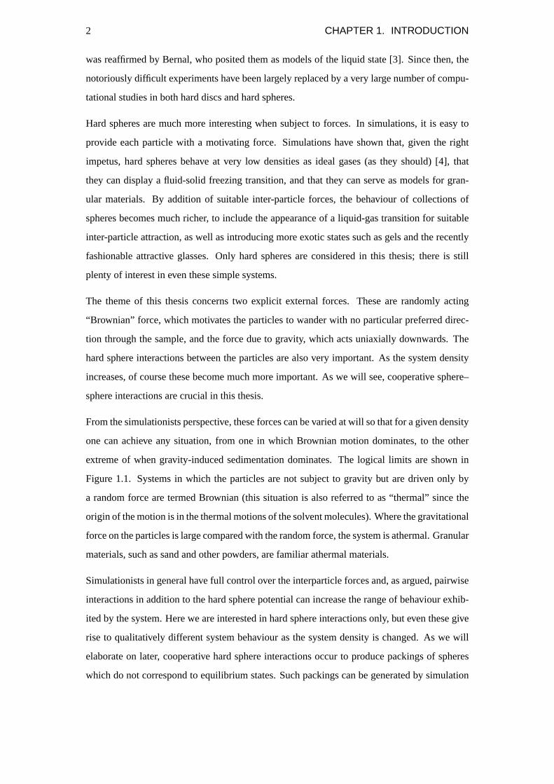
From the simulationists perspective, these forces can be varied at will so that for a given density
one can achieve any situation, from one in which Brownian motion dominates, to the other
extreme of when gravity-induced sedimentation dominates. The logical limits are shown in
Figure 1.1. Systems in which the particles are not subject to gravity but are driven only by
a random force are termed Brownian (this situation is also referred to as “thermal” since the
origin of the motion is in the thermal motions of the solvent molecules). Where the gravitational
force on the particles is large compared with the random force, the system is athermal. Granular
materials, such as sand and other powders, are familiar athermal materials.
Simulationists in general have full control over the interparticle forces and, as argued, pairwise
interactions in addition to the hard sphere potential can increase the range of behaviour exhib-
ited by the system. Here we are interested in hard sphere interactions only, but even these give
rise to qualitatively different system behaviour as the system density is changed. As we will
elaborate on later, cooperative hard sphere interactions occur to produce packings of spheres
which do not correspond to equilibrium states. Such packings can be generated by simulation

1.1. SPHERE PACKINGS ARE INTERESTING 3
Figure 1.1: A schematic representation of the various sphere packings considered in this thesis. Thehorizontal axis represents changes in system density. The vertical axis represents difference importanceof gravity. Also shown is a tentative link between the solid-like “colloidal” glass and sediments of systemsthat are not truly thermal.
methods such as molecular dynamics, but obviously are not predicted by equilibrium methods.
In particular, changes in system number density (“density quenches”) are important. This is
also shown schematically in Figure 1.1.
Sphere packings in all regions of Figure 1.1, as well as for more general potentials (not least
the emerging interesting cases of externally applied fields, for example, shear, optical and con-
fining walls) are interesting. However, there are two experimentally realisable sets of systems
which are particularly relevant here. The first is that of colloidal systems, a relatively new field
which provides a rich and exciting series of highly tunable model systems. The second is that
of granular matter, which, despite its venerability, still presents considerable theoretical and
experimental challenges. We discuss each below.
1.1.1 Colloidal Systems
Colloidal systems, or colloids, are usually described as being complex fluids in which at least
one constituent phase has a “mesoscopic” lengthscale; meso- implies middle, and is usually
taken to mean midway between the nanometer and micrometer scales. This condition and
these lengthscales are not themselves crucial; they ensure that

4 CHAPTER 1. INTRODUCTION
Dispersion Disperse Examples
medium phase TermNatural Biological Industrial
Clouds, mist, Hair spray,Liquid Aerosol
tobacco smokeCough
smogGas
Solid Aerosol Volcanic smoke Pollen Inhalation
Vacuoles, Shaving foam,Gas Foam Polluted rivers
insect excretions whipped cream
Biological Margarine, paint,Liquid Emulsion Milk
membranes vinaigretteLiquid
River water, Paint, ink,Solid Colloidal sol
mudBlood
toothpaste
Gas Solid foam Pumice, zeolites Loofah Styrofoam, zeolites
High impact plastics,Liquid Porous material Opals Pearls
ice creamSolid
Solid Solid suspension Wood Bone Pigmented plastics
Table 1.1: Types of colloids with some familiar examples. From [5].
(i) the colloidal particles are sufficiently large that individual interactions between
them and the solvent molecules are not significant (the solvent is considered
continuous) and that quantum effects can be neglected, and
(ii ) the force due to gravity is insignificant when compared with those imposed on
the particle by the solvent.
In the light of the introductory discussion above, we recognise that colloidal systems are any
real systems in which the particulate (mesoscopic) phase displays only Brownian motion. In
practice, this means the conditions above hold. It says nothing of the phase of the disperse or
dispersion media, which may in general consist of any combination of solid, liquid, or gas. To
illustrate the range and applicability of colloidal systems, and as is now traditional in theses
of this sort, Table 1.1 shows a variety of colloidal systems. Although in general any shape of
particle can be colloidal, in this thesis we consider only spheres. We hereinafter refer to these
spheres as colloids. Furthermore, we will study only solid spheres in a liquid medium.
1.1. SPHERE PACKINGS ARE INTERESTING 5
Interestingly, the word “colloid” is derived from the Greekκoλλα, which means glue. This
is a reflection of the fact that many practical colloids aggregate readily and is only barely
appropriate to their current accepted definition. We will discuss colloidal aggregation, and
particularly how it is avoided, shortly.
Why Study Colloids?
The most prosaic justification for studying colloids is that they provide a real system against
which the predictions of simulations can be judged. As we have argued, these are interesting in
their own right. As a specific example, it is hard not to be impressed when watching, directly
with the aid of a microscope, the emergence of crystallites in a seething supercooled sample of
spherical particles.
Perhaps more interestingly, colloids make good models of atomic systems. It has been shown
that with relatively modest assumptions (especially that the solvent is continuous), thermody-
namic properties are formally the same as for atomic systems [6]. This presents one very clear
advantage. Colloids are very much larger than atoms but carry the same energy per particle.
They can therefore not only be seen directly (by optical microscopy) or indirectly (by light scat-
tering)1, but also have much longer structural relaxation times. Processes such as crystallisation
which occur on the pico-second timescale in atomic substances occur on laboratory timescales
(seconds to months) in colloidal systems. These processes can be followed in colloidal systems
where they could not possibly in atomic systems.
Colloids are therefore interesting and useful as models of fundamental processes. As Table 1.1
shows, they are also relevant in many industrial and everyday situations. They are important in,
for example, developing water-based paints which are safe and environmentally more palatable,
but whose properties as paints (for example, in ease of application and quality of coverage) have
not been as good as for oil-based paints. Similar stories exist for a range of products such as
cements and glues. They are important for hygiene and beauty products; creating ever more
effective beauty products at a rate even close to that of the hype provides ample promise of
funding for colloid scientists. Recently, food colloids have become more fashionable: where
anti-wrinkle, anti-aging creams have led, miraculous pro-biotic yoghurts have followed. In
particular, issues such as shelf life have become important, since separation of contents are
1Atoms can of course be visualised by analagous means, by electron microscopy and by neutron/x-ray scattering,but this is difficult, impractical and expensive.

6 CHAPTER 1. INTRODUCTION
Context Examples
Everyday nuts, rice, coffee (both beans and instant!), corn flakes, and coal
Industrial powders, pharmaceuticals, agricultural (cereals, fertilisers), traffic jams
Terrestrial sand dunes, avalanches, ice floes, tectonics
Cosmic ice and rock collisions in planetary rings
Table 1.2: Some examples of granular materials.
unpalatable to consumers even if the product remains viable.
Lastly, to satisfy even the most pragmatic, there are many natural processes which are inher-
ently colloidal. Amazingly, we now know Brownian motion is crucial in a variety of biological
processes, for example protein folding, and molecular motors [7]. Rather than simply being a
nice model system against which to test simulations and theories of atomic systems, or even as
guiding models for development of industrial and consumer products, colloidal processes are
vital in many processes fundamental to sustaining life.
1.1.2 Granular Systems
Granular systems are ones in which there is no thermal motion, so that other forces dominate.
In this thesis, and many practical situations, the other force is always gravity. Granular systems
comprise a large collection of discrete macroscopic particles, and are characterised by a loss of
energy during collisions between particles.
Granular matter can display properties similar to solids, liquids, or gases. For example, when
poured, dry sand appears much like a liquid; when shaken vigorously, it behaves as a gas. A
dune, however, is more nearly solid than anything else. Granular matter is therefore sometimes
referred to as a state in its own right.
The applicability of granular matter is staggering, ranging from everyday examples to galactic
ones (Table 1.2).
In this thesis, we really only discuss the “solid” granular materials, similar to the pile of sand
in the bottom of an hourglass. However, even these display very complex behaviour. Not only
is the nature in which the load is borne in the packing complicated (the stress distribution is
highly inhomogeneous), but they display “fragility”, or an extreme sensitivity to loads other

1.2. “NEARLY THERMAL” SYSTEMS 7
than gravity (piles of dry sand are liable to avalanche in response to a very slight mechanical
disturbance) [8, 9].
Why Study Granular Matter?
The question of why to study granular matter almost answers itself; its broad applicability
makes it inevitably interesting. To be more specific, we note some remarkable facts [10].
Firstly, it is estimated that half of all products and three quarters of raw materials in the chem-
ical industry are in granular form, and that tens of billions of dollars are directly involved in
the technology required to handle these substances. Phenomena such as jamming in pipes
mean that a better understanding of these materials could make these tasks substantially more
efficient.
Moreover, the peculiar properties of granular materials are heavily implicated in their safe han-
dling. More than1000 hoppers, silos and bins fail annually in North America alone. More
disturbingly, the unpredictable nature granular piles results in frequent deaths from asphyxia-
tion, as workers walking on them trigger sudden rearrangements.
In addition to the clear industrial benefits that a better understanding of granular materials
would bring, it also has an inevitable draw for the physicist, who remains fascinated by hard
sphere systems. As de Gennes says in an article which describes well the interest for physicists
in granular matter, “granular matter, in 1998, is at the level of solid-state physics in 1930.”[8]
In other words, there is plenty of interest in even these apparently simple systems.
We do not actually study any granular systems in this thesis, but we do investigate how methods
used in their study are appropriate to our colloidal systems.
1.2 “Nearly Thermal” Systems
Although theories and simulations on sphere packings can explore any balance of thermal and
gravitational forces, most studies have concentrated on systems which are firmly in one regime
or the other. This is because there are relatively few real systems which lie part way between
the two. In most practical situations, the transition from thermal to athermal systems occurs for
a surprisingly small increase in particle size (an order of magnitude increase in particle radius
typically spans this crossover).
8 CHAPTER 1. INTRODUCTION
As we will discuss, however, practical colloidal systems often show behaviour which cannot
be explained by Brownian forces alone. Recently, some authors have begun to suggest that
applied forces on colloidal systems can induce arrested states of the sort seen in experiments.
This thesis considers a particular aspect of this suggestion by applying ideas from simulations
of granular matter to both some truly colloidal and “nearly colloidal” samples.
1.3 Thesis Layout
In general outline, this thesis first discusses the application of quantitative confocal microscopy
to a particular experimental system of small spheres. It then describes a technique used in sim-
ulations of granular matter, and applies this to some sphere packings under varying conditions
of density and buoyant mass.
To be more specific, Chapter 2 describes in detail the current state of knowledge for sphere
packings under the two extremes of applied forces we have discussed, that is colloid physics,
and granular physics. It then discusses aspects of the, much smaller, body of work which
applies to systems intermediate between these limits.
Chapter 3 concerns the quantitative confocal microscopy of spherical colloids, and builds a
case for the image of a just-resolvable spherical particle by describing the imaging process in
detail. This includes practical considerations such as noise.
Chapter 4 uses this knowledge to discuss how to identify particle centres reliably, even in dense
collections of solidly-fluorescent particles. This involves all aspects from optimising image
capture parameters to obtaining best results from the established techniques. A major result
of this thesis, an objective quantitative measure of the reliability of each determined particle
coordinate, is developed here, and it is demonstrated that an iterative best-fit technique devel-
oped around this measure, though still not necessarily optimised fully, can provide substantial
improvement to real images.
Chapter 5 is a straightforward description of the samples used and experimental conditions. It
also provides some simple characterisation of the particles used here.
Chapter 6 describes how to find bridges, the central analysis tool that is used in exploring the
thesis. It discusses some important parameters and elaborates on the basic results.
Chapter 7 presents the results of the bridging analysis on samples subject to normal gravity.

1.3. THESIS LAYOUT 9
Chapter 8 presents the same analysis as in Chapter 7, but for a system in which the effect of
gravity has been reduced by∼103, by nearly-matching the density of the solvent with that of
the particles.
In Chapter 9 we discuss fairly extensively further work which could be done on characterising
the bridges, but also note several key problems which must be considered in the bridging analy-
sis. In light of these, which follow from the results of Chapters 7 and 8, we suggest experiments
which those who simulate granular matter may be interested to try.

10 CHAPTER 1. INTRODUCTION

Chapter 2
Hard Spheres
In this Chapter we discuss all of the relevant properties of hard spheres, as used in this the-
sis. We first discuss collections of spheres, orpackings; this is a very general description,
and, to set the tone for this thesis, is a description of purely geometric properties of these sys-
tems. Next we discuss the behaviour of thermal systems, and some colloidal systems which
approximate these well. Following this we consider the other extreme of athermal (granular)
systems. We discuss how real systems fall between these limits, and how this is useful in some
circumstances. Lastly, we outline some speculative ideas which have been posited to explain
the apparent similarity of phenomena from all of these hard sphere regimes.
The hard sphere interaction
In all of what follows, we consider the spheres to interact with a purely hard sphere interaction
(although we discuss at times how real systems can vary from this idealisation). Figure 2.1
shows the interaction potential for genuine hard spheres. Spheres for which this pair potential
holds exert no influence on one another except when really in contact. When they do so, their
perfect rigidity ensures no deformation or overlap.
2.1 Packings
We almost manage to limit this discussion of the properties of packings of spheres to only
what is directly relevant to this thesis, although it is almost impossible not to discuss some
important and fascinating related results on packings of hard spheres. It never fails to amaze
11

12 CHAPTER 2. HARD SPHERES
0 2R
U(r)
r
∞
Figure 2.1: Ideal hard (monodisperse) sphere pair potential U(r) where r is the centre-centre separationand R is the particle radius.
the author that there have been vast numbers of experimental and numerical investigations into
these seemingly simplest of systems, yet their behaviour under even the simplest circumstances
is barely understood.
In this Section, we introduce some generic measures which are used to describe sphere pack-
ings, as well as some relevant alternative measures. We then discuss the important Random
Close Packed state, or more correctly, how it has been superseded, and extend upon this to
discuss in more detail what is required for a collection of spheres to be considered “jammed”.
2.1.1 Packing Fraction
The single most important parameter in packings of spheres, and the one jargon word most
likely not to be explained, is thevolume fraction, or packing fraction, denotedΦ. This is a
very simple concept, and is the total volume of the available volume which is occupied by the
particles:
Φ =Vparticles
Vavailable.
In the case where the particles are spheres, the volume fraction is
Φ =4πR3N
3V,
whereN is the number of particles,R is their radius, andV represents the volume available to
them.
In systems of hard spheres, the pair potential is not dependent on temperature; temperature
therefore has no effect on the phase behaviour, and from this point of view,Φ is the sole
important parameter.

2.1. PACKINGS 13
2.1.2 Important Packings
While Φ is the only important parameter in determining equilibrium phase behaviour, it cer-
tainly does not describe the system fully. In this Section we discuss two particularly important
types of packing.
Crystalline Packings
The first is where the particles adopt a crystalline arrangement. This is a familiar arrangement,
and turns out to be the stable state in a number of situations. The close-packed crystal, or
cannonball (or greengrocer’s oranges, if you prefer) stacking arrangement has the distinguished
status of having simultaneously the highest possible density,Φ = π3√
2' 0.7405, of any sphere
packing in three dimensions1 [11, 2], and the maximum number of contacting neighbours in
three dimensions (12). This latter requirement has also been a controversial one; Isaac Newton
and David Gregory debated this, also in the 17th century (Newton was right in this instance)
[1].
Crystalline packings need not be close packed; they can exist down to arbitrarily low densities.
Remarkably, crystallisation atΦ < 0.74 does not require anything other than a hard sphere
repulsion , although very low volume fraction crystals do require a repulsive component in the
pair potential (see Section 2.2.1 for an explanation). We do not need for this thesis to consider
crystals in any more detail; for further information see [5], or any standard crystallography text.
Random Close Packing
Much more interesting to us are random packings, and in particular, very dense random pack-
ings. The most dense random packing of spheres possible has traditionally been known as
Random Close Packing, or RCP, and has been studied to a quite remarkable extent.
The RCP state became famous through the work of Bernal and his co-workers. The most
famous of these is the Bakerian lecture of 1962 [3], in which he described a random close
packing as a “heap”, as opposed to a “pile”, his designation for an ordered packing. A heap is
in his description a “casual and unstable” packing. The focus of the article is in attempting to
1As Kepler said: “The packing will be the tightest possible, so that in no other arrangement could more pelletsbe stuffed into the same container.” [2] It took more than350 years for this fairly inoffensive assertion to be provedcorrect.

14 CHAPTER 2. HARD SPHERES
explain the structures of liquids, and this article is a fairly good review of some of the at that
time state of the art computer simulations and experiments which he and others performed.
These included the first paper on this topic [12, also [13]], in which he investigates heaps which
are necessarily liquid due to their substantial regions of five-fold symmetry (which precludes
long-range order). This paper sets a precedent for eye-wateringly painstaking experiments, typ-
ified by the experiments of his PhD student Mason, who stuck thousands of 1/4” ball bearings
arranged in a near-RCP state in paint, then prised the arrangement apart, noting the number of
contacts and near contacts for each sphere [14]. For an interesting machine for determining
sphere coordinates in random packings, see [15]. Amongst Bernal’s many other papers are one
on the emergence of order from random packings under shear [16], and an explanation of the
heat of fusion of Argon based on its being well-modelled by a random hard sphere packing
[17].
Other prominent papers from the early days of random packings include those of Scott and
(separately) Mason, who attempted to find the structural properties of (that is, quantify spatial
distributions of spheres in) these packings [18, 19, 20]. The papers of Finney provide more
detail of this work on liquid structure and heats of fusion, [21] and [22] respectively.
The above list is a very short one, and certainly misses out many deserving papers. For a
respected review, please see [23]; also [24] is useful.
As computers have become more powerful, simulations have become more useful. The work
of Jodrey and Tory deserves mention, [25, 26, 27, 28]; their simulations and analysis are a
significant advance over the earlier papers.
However, the most widely used and best option for generating sphere packings is the algorithm
of Lubachevsky and Stillinger, which produces large random packings efficiently using an
event-driven molecular dynamics procedure [29, 30, 31]. Briefly, this algorithm starts with
randomly-positioned point particles (that is, an ideal gas) which move around with random
velocites, and interact purely via a hard-sphere potential. It then grows the particles in time,
thereby increasing the system density. Ultimately the system becomes jammed into a final
state which depends on the particle growth rate; fast growth results in a final volume fraction
of Φ'0.64. For some further details on our implementation of the Lubachevsky-Stillinger
algorithm, please see [32], although this is not used in this thesis.
Scott is the first author of whom we are aware to identify explicitly an important counterpoint
to RCP, namelyRandom Loose Packing, RLP [33]. The arguments which lead to the no-

2.1. PACKINGS 15
tion of RCP lead to an intuitive understanding of what RLP is; essentially it is a “heap”, as
Bernal would have it, which is minimally dense whilst remaining mechanically stable (against
gravity). This is as opposed to RCP, which is the densest possible random packing, and is to
some extent incidentally able to bear a load. RLP is even less well understood than RCP, but it
seems somehow less general than RCP, being presumably stable against only gravity, whereas
RCP packings are presumably stable against a broader range of forces. (As an example, the
Lubachevsky-Stillinger algorithm, for which the forces are random and isotropic, cannot pro-
duce random loose packings, only dense ones.) That there can be more than one sense in which
a sphere packing is stable is an important point, and we return to this later.
Despite the huge number of publications on the RCP state, it is still an unsatisfying concept,
and the variability reported in the various studies described above rightly suggest that it is not
a well founded concept. We return to this later in this Chapter, but first discuss how we can
distinguishing between different packing types.
2.1.3 Radial Distribution Function, g(r)
The most widely-used structural descriptor of packings of spheres whose coordinates are known
is the radial distribution function , also known as thepair distribution function , the pair
correlation function or simply g(r). It describes the probability of finding other particles at
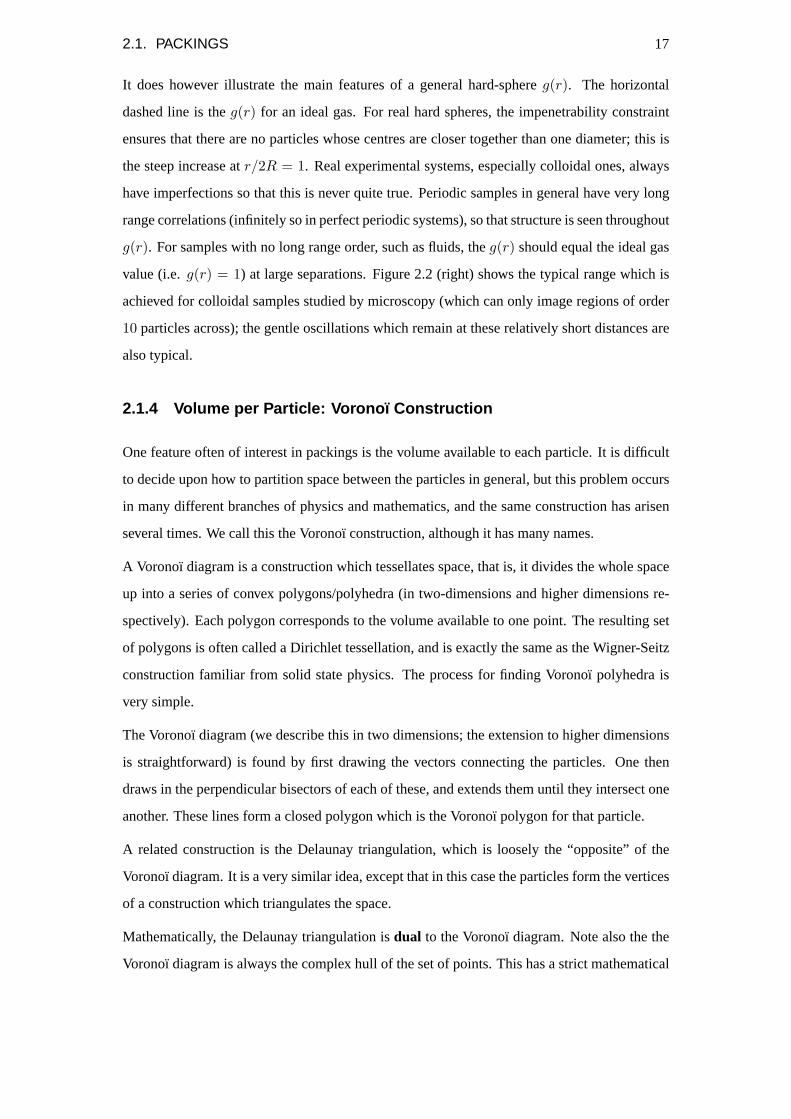
a given centre-to-centre separation from any randomly-chosen particle. Figure 2.2 helps to
explain this. Figure 2.2 is a two-dimensional representation of a fairly dilute and apparently
i ijjr
drg(r)
10
1
r / 2R
Figure 2.2: Explanation of how g(r) is constructed (left), and a schematic example illustrating its importantfeatures (right).
amorphous collection of spheres. This corresponds to a colloidal hard sphere (relatively dense)
gas. The pair distribution function g(r) is the probability of finding a particle at a given sepa-
ration r, that is, it is the number of particles at a given distance from a test particle normalised

16 CHAPTER 2. HARD SPHERES
by the same quantity in the ideal gas (i.e. non-interacting particles) of the same density. The
number of particles in a thin shell of widthdr as indicated is (in three dimensions):
Nshell = ρVshell × g(r) = 4πr2ρg(r)dr.
In practice, g(r) is calculated by finding the distance between each pair of particles and placing
these into a correct bin (choosing the size of the bins specifies the precision to which g(r) is
found). The number of particles that would be in this shell in the ideal gas is then4πr2ρdr,
whereρ is the number density of the colloids and is known (the volume of and the number of
particles in the sample are both known). The pair correlation function is then
g(r) =Number in shell at current r
4πr2ρdr.
It is worth noting that the essential information in g(r) is present even if the distribution is
not normalised. An attempt to show this is given in Figure 2.3. The normalisation is essen-
g(r)
10 r / 2R
Figure 2.3: Schematic illustration of unnormalised version of g(r), which is simply the number of particles,N(r), found in a spherical shell of thickness dr and radius r. The dashed line represents the “ideal gas”r3 dependence.
tially simply dividing g(r) byr3, so omitting the normalisation gives the “useful” distribution
superimposed on anr3 curve. In this representation, it is more difficult to discern structural
information, and it is considered less useful here. Some authors distinguish these two repre-
sentations by reserving one of “pair correlation function” and “pair distribution function” for
each2. This makes sense, but there is some confusion. In this thesis, only the normalised
version is considered, and the terminology used interchangeably.
The right-hand image in Figure 2.2 is an exampleg(r). It is not meant to represent any real
system, particularly it is not meant to be close to theg(r) for the left-hand image in this Figure.
2Specifically, “pair correlation function” is more often the normalised version, whereas “pair distribution func-tion” is the unnormalised one.
2.1. PACKINGS 17
It does however illustrate the main features of a general hard-sphereg(r). The horizontal
dashed line is theg(r) for an ideal gas. For real hard spheres, the impenetrability constraint
ensures that there are no particles whose centres are closer together than one diameter; this is
the steep increase atr/2R = 1. Real experimental systems, especially colloidal ones, always
have imperfections so that this is never quite true. Periodic samples in general have very long
range correlations (infinitely so in perfect periodic systems), so that structure is seen throughout
g(r). For samples with no long range order, such as fluids, theg(r) should equal the ideal gas
value (i.e.g(r) = 1) at large separations. Figure 2.2 (right) shows the typical range which is
achieved for colloidal samples studied by microscopy (which can only image regions of order
10 particles across); the gentle oscillations which remain at these relatively short distances are
also typical.
2.1.4 Volume per Particle: Voronoı Construction
One feature often of interest in packings is the volume available to each particle. It is difficult
to decide upon how to partition space between the particles in general, but this problem occurs
in many different branches of physics and mathematics, and the same construction has arisen
several times. We call this the Voronoı construction, although it has many names.
A Voronoı diagram is a construction which tessellates space, that is, it divides the whole space
up into a series of convex polygons/polyhedra (in two-dimensions and higher dimensions re-
spectively). Each polygon corresponds to the volume available to one point. The resulting set
of polygons is often called a Dirichlet tessellation, and is exactly the same as the Wigner-Seitz
construction familiar from solid state physics. The process for finding Voronoı polyhedra is
very simple.
The Voronoı diagram (we describe this in two dimensions; the extension to higher dimensions
is straightforward) is found by first drawing the vectors connecting the particles. One then
draws in the perpendicular bisectors of each of these, and extends them until they intersect one
another. These lines form a closed polygon which is the Voronoı polygon for that particle.
A related construction is the Delaunay triangulation, which is loosely the “opposite” of the
Voronoı diagram. It is a very similar idea, except that in this case the particles form the vertices
of a construction which triangulates the space.
Mathematically, the Delaunay triangulation isdual to the Voronoı diagram. Note also the the
Voronoı diagram is always the complex hull of the set of points. This has a strict mathematical

18 CHAPTER 2. HARD SPHERES
definition, but is basically the largest volume which drawn using points in the packing. For a
comprehensive book on Voronoı diagrams and their application in the field of computational
geometry, see [34].
2.1.5 Other structural descriptors
The radial distribution function is a useful and widely used measure of the structure of a pack-
ing, not least because it is closely related to the structure factor, a property which is readily
available in scattering experiments. Although we use it here, it is not ideal, since it is an av-
erage property; it describes the probability of finding a particle at a given radial distance from
another particle, but contains no angular information. Moreover, it is reasonably insensitive to
structural changes (as we show later, g(r) for a glass atΦ ' 0.62, say, is very similar to that for
a (supercooled) liquid atΦ ' 0.55, say; this is especially true when small experimental errors
are present).
Local Bond Order Parameters
Local structural information is often desired. Some studies have been done on the angular ori-
entation of nearest neighbour bonds in RCP [25, 26, 19], but these have not been widely used.
One particular set of orientational order parameters which have been used quite extensively
are those introduced by Steinhardtet al. [35, 36]. These are rotationally invariant (so that the
relative orientation of any structures within the sample, and their overall orientation with re-
spect to the laboratory, is not important) combinations of spherical harmonics. There are many
possible combinations, and typically the so-calledq4, q6, andw6 are sufficient. It turns out
that these have different values for different structures, and they can be used to differentiate be-
tween crystal types using an essentially fingerprinting method. These are useful and powerful
measures, and have been useful in investigating crystallisation in colloidal systems [37, 38].
Void Space and Remoteness
Although we do not consider it in detail in this thesis, it is worth mentioning the concept of
void space. In sphere packings, the volume fraction never exceedsΦ ' 0.74; the remaining
space isvoid space. Rather than the volume fraction, some authors prefer to try to explain
sphere packing phenomena in terms of the space available in the packing [39]; this makes

2.1. PACKINGS 19
intuitive sense since presumably dynamical arrest is related to how much space is available for
individual particles to move.
It is in general difficult to define void space since although the narrow channels between par-
ticles are clearly void space, they are not usually as interesting as larger voids, for example
those into which a particle could fit. The distinction is somewhat arbitrary, but the quantityre-
motenessgoes some way to helping this. The remoteness of a point in the sample is simply the
distance from it to the surface of the nearest particle. The remoteness is set to zero for all points
inside the particles. In practice, remoteness is calculated for a large number of randomly-placed
points in the sample. The resulting distribution gives information on the distribution of void
space in the sample.
Remoteness has been used to investigate simulated aggregates [40], and in studying local den-
sity fluctuations during hard sphere crystallisation [41]. Note also that remoteness is very
similar to the measure of void space distribution (“Pore-Size Functions”) introduced by Prager
([42], §5.1.6)
2.1.6 Is Random Close Packing Well Defined?
This Section shares its name with a paper by Torquatoet al. [43], which, along with many
other papers from his group, discusses dense random packings in considerable detail. Here we
discuss briefly how the notion of RCP is inadequate in describing very dense random packings.
In this paper, Torquato reiterates the traditional view of RCP as being the following: “ball
bearings and similar objects have been shaken, settled in oil, stuck with paint, kneaded inside
rubber balloons—and all with no better result than (a packing fraction of) ...0.636 [44, cited
in [43]]. They also note the large variation in density that these methods have suggested for the
random close packed volume fractionΦRCP .
Their conclusion to this is that RCP is not well defined. One of the examples they cite helps
to explain this. Scott and Kilgour, in one classic experiment, expressly vibrated their system
as they poured ball bearings into a container [45]. The vibration, particularly when bearing in
mind the observation cited earlier that shear induces order [16], reveals the important point that
the terms “random” and “close packed” are at odds
with one another.

20 CHAPTER 2. HARD SPHERES
Imagine a RCP sample, at volume fractionΦ ' 0.64, as envisaged by Bernal. One can then
easily imagine introducing a small amount of order (a small crystallite). Such a region can
be arbitrarily small, but will always increase the volume fraction. Rather than random close
packing, Torquatoet al. [43, 46] suggest that what we really seek is theMaximally Random
Jammedstate. They suggest that there is anorder parameter–volume fraction plane, Figure
2.4, in which all sphere packings reside.
Figure 2.4: The order parameter versus volume fraction plane. The black line is the locus of jammedstates. Point A is the lowest volume fraction jammed structure, B the close-packed crystal, and MRJ themaximally-random jammed state. Taken from [43].
In these papers, Torquatoet al. argue that it should be possible to define a measure of order
(designatedψ in Figure 2.4) which places any packing somewhere along the vertical axis. They
do not have a perfect order parameter, although they discuss a number of options including
the bond order parameters (particularlyq6) described above. They then classify a system as
jammed with the two statements (quoting [43]):
• a particle is jammed if it cannot be translated while fixing the positions of all of the other
particles in the system, and
• the system itself is jammed if each particle (and each set of contacting particles) is
jammed.
This definition of jammed gives rise to a locus of jammed states, as indicated in Figure 2.4.
Note that this is schematic and almost certainly not right. For example, it is possible to get a
mechanically stable (and therefore jammed) packing of volume fraction as low as0.055 [1].
The point is well made by Figure 2.4, however. Note also that this locus is exclusively for hard
spheres; it does not consider jammed systems with additional interactions (for example gels).

2.1. PACKINGS 21
In this Figure, three important points are illustrated. The first is Point B, which is the close-
packed crystal. This is straightforwardly jammed, and is both dense and highly ordered, so
occupies the upper right of the plane. Point A is the lowest volume fraction which is jammed,
and may represent the RLP state (although the RLP state usually is reserved for packings stable
against a very particular applied force, namely gravity, rather than being “truly” jammed). The
point marked “MRJ” is the least ordered jammed state which can occur; this seems to me to be
fairly self-evidently associated with what others have sought when describing RCP.
We should note that despite the sense which papers seem to make, they have been disputed.
O’Hern and co-workers have talked in terms of what they call “Point J”, a similar concept
[47, 48], but since they vociferously advocate the use of soft potentials in their simulations3, a
debate has ensued [49, 50]. It seems hard to argue with Torquatoet al.; their scheme is simple
and apparently indisputable.
Jamming Categories
Torquato’s group go further, however, by showing that there is a hierarchy of jamming cate-
gories. They discuss how the concept of jamming is subtle, and not itself well-defined in the
literature (the above definition is not sufficient). We do not really discuss these in great detail
in this thesis, but they are relevant and we do mention them in passing. As stated by Torquato,
a system ofN spheres is said to be a
• locally jammed configurationif the system boundaries are nondeformable and each of
theN particles is individually jammed
• collectively jammed configurationif the system boundaries are nondeformable and it
is a locally jammed configuration in which there can be no collective motion of any
contacting subset of particles that leads to unjamming
• strictly jammed configurationif it is collectively jammed and the configuration remains
fixed under infinitesimal virtual global deformations of the boundaries. In other words,
no global boundary-shape change accompanied by collective particle motions can exist
that respects the nonoverlap conditions.
3Bizarrely, they question whether the hard sphere system used by Torquato is “physical”. One can only wonderwhat they mean by this.

22 CHAPTER 2. HARD SPHERES
They subsequently illustrate which of these categories each of a wide range of familiar packings
falls into, and these can be quite surprising; for details, consult these references.
Whatever the exact definition, the states we have discussed are certainly at least locally jammed,
which means that no particles are free to move. In practice, most, and we would argue es-
sentially all, practical (both simulated and experimental) packings will include at least some
particles which are not jammed according to the above definition. These particles are termed
rattlers , and a population up to around5% are widely reported in simulated packings (see for
example [43]). Some may argue that such rattlers fall within the definition of RCP, but we
would argue a system with rattlers is at best an approximation to a “true” RCP state. There
is no ambiguity in the MRJ state, which have strictly no rattlers. Of course, any ambiguity
in whether RCP allows the presence of rattlers simply reflects that it is an insufficiently well-
defined concept.
2.2 Thermal Systems
We now discuss thermal systems, in which the only forces motivating the particles are Brown-
ian and the hard-sphere repulsion. Even in this very simple system, interesting and surprising
behaviour emerges.
2.2.1 Phase behaviour of ideal hard sphere systems
The phase behaviour of perfectly hard spheres subject to Brownian motion has been established
by computer simulation, and have been complemented by phenomenological analytic models
which agree remarkably closely with these simulations.
Numerical simulations have been used to establish the hard sphere equation of state. Wood
and Jacobson showed that even though the the pair potential is (very!) short-ranged, hard
sphere systems exhibit a disorder-order transition [51]. The fluid phase has no long range order,
whereas the solid phase adopts a crystalline arrangement which does display long-range order.
Subsequently, Hoover and Ree showed that there is a freezing transition,Φf , at Φ = 0.494,
and a melting transition,Φm, atΦ = 0.545 [4]. Below Φf , the equilibrium state of the system
is fluid; aboveΦm, the system is in equilibrium when it is fully crystalline. ForΦf ≤ Φ ≤ Φm,
the system comprises coexisting fluid and solid regions; in this case an appropriate amount of
2.2. THERMAL SYSTEMS 23
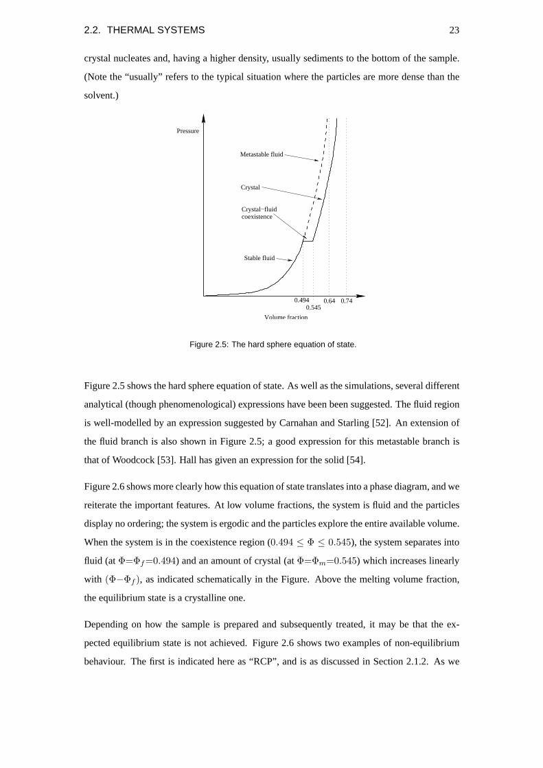
crystal nucleates and, having a higher density, usually sediments to the bottom of the sample.
(Note the “usually” refers to the typical situation where the particles are more dense than the
solvent.)
0.740.64
Stable fluid
Crystal
Metastable fluid
Crystal−fluidcoexistence
Pressure
0.494
Volume fraction
0.545
Figure 2.5: The hard sphere equation of state.
Figure 2.5 shows the hard sphere equation of state. As well as the simulations, several different
analytical (though phenomenological) expressions have been been suggested. The fluid region
is well-modelled by an expression suggested by Carnahan and Starling [52]. An extension of
the fluid branch is also shown in Figure 2.5; a good expression for this metastable branch is
that of Woodcock [53]. Hall has given an expression for the solid [54].
Figure 2.6 shows more clearly how this equation of state translates into a phase diagram, and we
reiterate the important features. At low volume fractions, the system is fluid and the particles
display no ordering; the system is ergodic and the particles explore the entire available volume.
When the system is in the coexistence region (0.494 ≤ Φ ≤ 0.545), the system separates into
fluid (at Φ=Φf=0.494) and an amount of crystal (atΦ=Φm=0.545) which increases linearly
with (Φ−Φf ), as indicated schematically in the Figure. Above the melting volume fraction,
the equilibrium state is a crystalline one.
Depending on how the sample is prepared and subsequently treated, it may be that the ex-
pected equilibrium state is not achieved. Figure 2.6 shows two examples of non-equilibrium
behaviour. The first is indicated here as “RCP”, and is as discussed in Section 2.1.2. As we

24 CHAPTER 2. HARD SPHERES
saw there, this is a controversial designation, but something similar certainly occurs in colloidal
systems. The second is the so-called glass transition, and is also still disputed. It occurs at a
volume fraction between the melting point and the point marked “RCP”. The evidence for a
glass transition is overwhelmingly experimental; we discuss this further in Section 2.2.4.
0.74
Volume fraction
0.494 0.545 0.58 0.64
% crystal
100%
0%
Glass RCP
CrystalFluid + crystalFluid
Figure 2.6: A schematic phase-diagram for hard spheres. See text for details.
Hoover and Ree ([4]) showed that the disorder-order (freezing) transition is driven by entropy.
It is not obvious that hard spheres should adopt arrangements with long-range order when they
have no long-ranged interactions; the explanation lies in the competition between the so-called
global (or configurational) and local (or free volume) entropies.
Figure 2.7: A two-dimensional illustration of the mechanism behind entropy-driven freezing of hardspheres. Despite being more ordered, the right-hand system has higher overall entropy due to its higherfree volume entropy. See text for fuller explanation.
Figure 2.7 helps to explain this. The left-hand image in this Figure displays a (two-dimensional)
2.2. THERMAL SYSTEMS 25
liquid-like arrangement of particles. This situation, which shows no order, can occur up to
the maximally dense disordered volume fraction ofΦ'0.64. At around this point, all of the
particles become arrested. In this situation, the particles are not free to move; this is another
way of stating that they no longer have free volume entropy.
We naturally expect the system to adopt the state of highest entropy, and since this is usually
loosely referred to as a measure of disorder, our intuition leads us to expect disordered states,
which indeed do have lower configurational entropy. It turns out that the better packing ef-
ficiency of an ordered state over a disordered one for spheres means that the increase in the
free volume entropy per particle this affords more than offsets the reduction in configurational
entropy due to crystallisation.
The volume fraction at which a hard sphere system crystallises therefore occurs when the de-
crease in the configurational entropy is more than offset by the increase in the free volume
entropy.
2.2.2 Hard sphere model systems
There are many real systems which can be used to approximate the hard sphere systems de-
scribed above. No real system does this perfectly, and in this Section we discuss the most
prominent departures from the ideal behaviour, and how these can be dealt with.
van der Waals attractions
The tendency of colloids which originally gave them their name arises from the van der Waals
attractions which act between them. The van der Waals force is ubiquitous in colloidal systems,
since it originates in the interaction between the fluctuations of electrons within the atoms and
molecules of which the colloidal particles are made. The basic idea is that a fluctuation in the
charge distribution of one molecule will leave it slightly charged (positively, for the sake of
argument) at one end. A nearby molecule will experience a field which polarises it (in this
case, with the positive charges pushed away from the first molecule). This results in a positive
(on the first molecule) and a negative (on the second) being close together, and therefore there
is a net attraction. For a more convincing description of this process, see Israelachvili [55].
For two atoms, the interatomic attraction goes asr−6, wherer is the separation of the atoms.
Colloidal spheres obviously contain (a large number of) atoms, all of which interact with one
26 CHAPTER 2. HARD SPHERES
another. By assuming pairwise additivity and summing over pairs of atoms, the potentialU(r)
between two spheres due to the van der Waals attraction can be shown to be [56]
U(r) = −A
6
[2R2
r2 − 4R2+
2R2
r2+ ln
(1− 4R2
r2
)],
whereA is the Hamaker constant. Since the origin of the van der Waals force is in the fluctu-
ating dipole moments of the constituent atoms, it is not surprising that the Hamaker constant is
related to the polarisability of the particles and solvent and therefore their respective permittiv-
ities εc andεs:
A ∝(
εc−εs
εc+εs
)2
.
The prefactor in this relation is dependent on the geometry; for some examples, see [55].
The van der Waals force is therefore always attractive. It is possible to stabilise colloids against
aggregation by matching the index of refraction (n=√
ε) of the solvent and particles. In gen-
eral, the permittivities are frequency dependent, so this is not perfectly satisfactory, as well as
rendering the particles invisible. This may or may not be desirable depending on the measure-
ment technique employed.
At large distances,r →∞, we get
limr→∞U(r) = −16
9
(R
r
)6
,
which displays the requiredr−6 dependence. More interestingly in colloidal systems is the
limit as particles near contact:
limr→2R
U(r) = − A
12R
r − 2R.
This represents a deep minimum which can be several orders of magnitude larger than the
thermal energykBT [57], and so typically leads to the irreversible “glued together” aggregation
that gives colloids their name. To counteract this effect, the particles are commonly stabilised
against aggregation using eitherchargeor steric stabilisation.
Charge stabilisation
In some cases, colloidal particles have ionisable molecules at their surface, and when dispersed
in some solvents, these can dissociate. The liberated ions tend to diffuse away from the particle
by Brownian motion, leaving the initially neutral particle charged with the remnant ions. These
remaining ions influence the ions in solution (particularly if the solvent has added electrolyte)

2.2. THERMAL SYSTEMS 27
to prevent them from being distributed throughout the sample. The result, illustrated in Figure
2.8, is an electrical double layer around each particle which provides a repulsive contribution
to its interaction potential. The particle and its double layer are now termed macroion and
ion cloud, with the ion cloud comprising counterions (i.e. those liberated by the dissociation
at the particle surface) and any electrolyte ions. When two macroions approach one another,
their double layers must overlap. This causes a repulsive force which provides the desired
stabilisation.
Particlecore
Doublelayer
Particle core
Stabilisinglayer
Figure 2.8: Two types of stabilisation for colloidal particles: charge-stabilisation (left) and steric stabilisa-tion (right) stabilisation.
Debye Length
The counterions remain trapped by the electric field of the particle, but drift away under the
influence of Brownian motion. The result is a distribution of charges near to the surface of
the particle which gives rise to a varying potential. This potential can be found by solving a
linearised Poisson-Boltzmann equation (the Debye-Huckel equation):
UC(r) =(Qe)2
4πε0εr
exp[−κ(r−2R)](1+κR)2
,
where Q is the charge carried by each particle,e the electronic charge,ε0 the permittivity of
free space,ε the solvent dielectric constant, andκ−1 the so-called Debye screening length. The
Debye length is a measure of the extent of the double layer:
1κ
=(
εε0kBT
e2∑
z2i ni
) 12
. (2.1)
Here,ni is the number density of speciesi counterions in the bulk species andzi their valence,
kB is the Boltzmann constant,T is the temperature, and the sum is over all species of ion.
28 CHAPTER 2. HARD SPHERES
Steric stabilisation
Steric stabilisation is achieved by attaching polymer molecules to the surface of the particles.
The polymer molecules are of modest length, and attached at one end only to the particle. The
rest of the molecule is free to “wave” in the solvent. This “polymer brush” is illustrated in
Figure 2.8.
The polymer molecules perform Brownian motion in the solvent, but if the particles stray too
close to one another, the polymer brushes begin to overlap. As they interfere with each other’s
motion, there is an entropy cost, which gives rise to an osmotic force that tends to keep the parti-
cles apart. A fuller explanation of this effect becomes quickly complicated ([58, 59]). The basic
parameters are the surface density of the polymer molecules, whether the polymer molecules
are chemically attached to the particles, and how good a solvent the dispersion medium is for
the polymer.
Silica particles are frequently sterically-stabilised by chemically grafting onto them one of a
variety of suitable polymers [5]. Another, now widely studied, system is polymethylmethacry-
late (PMMA) colloids with poly-12-hydroxystearic acid (PHSA) polymer hairs. This is the
experimental system used here.
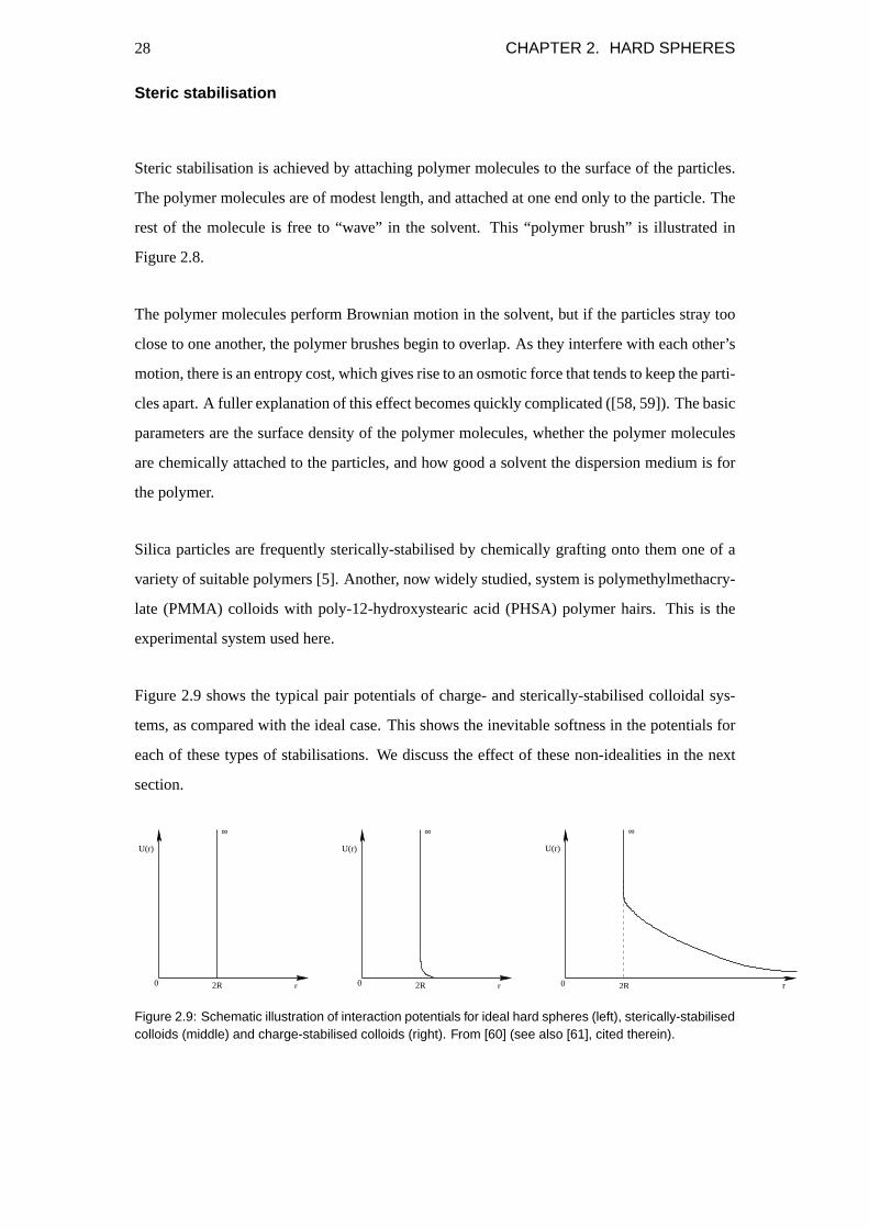
Figure 2.9 shows the typical pair potentials of charge- and sterically-stabilised colloidal sys-
tems, as compared with the ideal case. This shows the inevitable softness in the potentials for
each of these types of stabilisations. We discuss the effect of these non-idealities in the next
section.
0 2R
U(r)
r
∞
0 2R
U(r)
r
∞
0 2R
U(r)
∞
r
Figure 2.9: Schematic illustration of interaction potentials for ideal hard spheres (left), sterically-stabilisedcolloids (middle) and charge-stabilised colloids (right). From [60] (see also [61], cited therein).
2.2. THERMAL SYSTEMS 29
2.2.3 Limitations of colloidal systems
Hardness of interaction potential
The equilibrium phase behaviour of perfectly repulsive hard spheres is well known, but it varies
quickly as the pair potential is altered. The freezing and melting volume fractions are particu-
larly sensitive to variations in the interaction potential. The ratioΦM−ΦFΦF
is useful in assessing
how nearly a system approximates hard-sphere behaviour [62]. This ratio is approximately0.1
for hard spheres.
Importantly in this thesis, we note that for perfectly hard spheres, the closest distance of ap-
proach does not change with particle number density. Even at low volume fractions, there will
be some particles occasionally in (or very near to) contact. If the potential is soft, for example,
as in Figure 2.9 (right), then the particles tend to avoid each other and therefore the first peak
in g(r) will be at a relatively large separation. As the volume fraction and therefore the osmotic
pressure (Figure 2.5) increase, the particles are increasingly pushed closer together, so the first
peak of g(r) will be shifted to lower values. The importance of this is that the degree to which
the position of the first peak in g(r) moves gives an indication of the hardness of the interaction
potential.
Size polydispersity
The discussion so far has concentrated on systems in which all of the particulate phase are
exactly the same size, that is, the system ismonodisperse. In reality, with a few biological
exceptions (notably proteins and viruses e.g. FD virus), all practical systems have particles
with a range of sizes. This is particularly so of industrial systems.
The distribution of sizes is quantified by the measure (the “polydispersity”)
σ ≡
√R2 −R
2
R,
whereR is the mean particle size, andRn is thenth moment of the particle size distribution,
f(R), in the usual way:
Rn =∫
Rnf(R)dR.

30 CHAPTER 2. HARD SPHERES
The phase behaviour of polydisperse hard sphere systems is similar to that for the monodisperse
case for small polydispersities (σ . 0.06). For larger polydispersities (σ & 0.12), crystallisa-
tion is suppressed. For moderate polydisperties (σ ' 0.075-0.095), crystallisation occurs, but
very slowly. For much more detail on the effect of polydispersity, see [63] (in particular for a
justification of the [debatable] polydispersities). In this thesis, rapid crystallisation is taken to
imply a polydispersity of less than around6%. For the purposes of volume fraction determina-
tion, we use the mean particle radiusR. In later calculations, we account for polydispersity by
allowing a range of separations for contacting neighbours.
In this thesis we consider that the size polydispersity is the only significant variation between
particles. We assume that there is no distribution in asphericity (that is, the particles are as-
sumed perfectly spherical) and that, where appropriate, there is no charge polydispersity.
2.2.4 Evidence for nearly-hard-sphere behaviour in colloidal systems
Notwithstanding the limitations of real model hard sphere systems, there have been a large
number of studies performed on systems which behave convincingly well as hard spheres.
Systems of polystyrene and silica particles have been widely used, and under the right condi-
tions behave well as hard spheres (for example, [64] and [65] respectively, as cited in [57])
In this thesis, we use one particular system which has been studied in considerable detail.
This system comprises PMMA particles sterically stabilised by PHSA hairs and suspended
in decalin. Pusey and van Megan showed that this system behaves convincingly as a hard
sphere system, by displaying the correct relationship betweenΦf andΦm (Φm−Φf
Φf= 0.085,
convincingly close to the expected value of0.1), as well as a sediment volume fraction of
around the expectedΦ = 0.64 [66] (for more details, and further evidence of the hard sphere
behaviour of this system, see [5],§2.2.4).
The Glass Transition
Despite the evidence for the agreement between simulations of hard spheres and these model
systems, there is an important intriguing outstanding phenomenon. This was first mentioned
in Figure 2.6, where it was noted that in colloidal model systems, a glass is formed for volume
fractionsΦ & 0.58 (including in the seminal paper of Pusey and van Megan, [66]).

2.2. THERMAL SYSTEMS 31
This phenomenon is observed experimentally. Briefly, a glass is a state where short term,
small distance motions are much as expected in a liquid. Long term, large scale motions
are suppressed, however, and the sample, whilst remaining apparently fluid-like, ceases to be
ergodic. This behaviour has been well established using light scattering techniques [56, and
references therein].
The glass transition has so far not been understood. We should note that while computer simula-
tions show a clear jamming transition corresponding to the RCP state ([43, 29], and discussion
above), it is certainly not clear that a glass transition at lower volume fraction emerges from
simulation. Some claim that it does [67, 68], although this is still a matter for debate [69].
Prominent simulationists continue to claim that it does not [70].
There is substantial argument over what exactly the glass transition is. It is not even clear
whether the glass transition is thermodynamic, or simply dynamic. If the latter is true, then
the glass transition simply marks the point at which the observable diffusion occurs on a much
longer timescale than a reasonable experiment can run4. The uncertainty in the volume frac-
tion at which the glass transition occurs may reflect this (though this volume fraction is very
sensitive to experimental conditions such as polydispersity). In molecular glasses, the glass
transition is defined as having occurred when the sample viscosity has achieved some arbitrar-
ily chosen value.
This last comment reveals a lot about why colloidal glasses have become of considerable in-
terest. The basic picture of a molecular glass is of a frustrated liquid; it is seemingly what
you get if you cool a liquid to substantially below its freezing point so quickly that it does not
undergo the phase transition. Once in such a state, asupercooledliquid can be cooled further.
At some point, the substance in this state does not flow under applied stress, in which case it is
somehow more solid than it is liquid. This is a very much analogous situation to that described
for colloidal glasses above, and it has been hoped that colloidal systems, which are experi-
mentally much more accessible, may serve as an illuminating model for atomic and molecular
glass-formers. This description of vitrification is very crude, and the interested reader really
ought to read an authoritative article on the subject, for example [72].
To make the situation more complicated, one group has suggested that the colloidal glass tran-
sition may be due to gravity. This is a reasonable suggestion, and might explain why it is4For a nice relevant example of a system which seems to support the idea that the glass transition is purely a
timescale-related phenomenon, see [71]. In this experiment, pitch, a substance which is by everyday experienceclearly a solid (it cracks when subject to a hammer blow!), has continued to drip at a remarkably slow rate (aboutone drop every ten years) from a funnel.

32 CHAPTER 2. HARD SPHERES
not seen in simulations. Zhuet al. performed experiments on the Space Shuttle, and claim that
their samples showed no glass transition [73]. This was presumably quite a difficult experiment
to perform in a controlled manner, and is not sufficient evidence on its own. In support of this
result, however, Kegel [74] has reported a similar result by careful matching of the density of
the solvent with that of the particles. This is a more convincing result, although as yet we bear
in mind that these two results are still a small body of evidence. That gravity may be involved
in the glass transition is an important issue in this thesis.
The outstanding lack of understanding of the glass transition has frustrated colloid scientists for
some time. There is a large amount of high-quality light-scattering data available, but whilst
this technique has proved extremely useful so far, it suffers from the inherent disadvantage
that it can provide only average quantities from relatively large volumes of the sample. One
suggestion for an explanation of the glass transition is that flow in supercooled liquids involves
cooperative motion of constituents, and that the size of the clusters of cooperatively moving
constituents diverges at the glass transition [75]. Based on this suggestion, many theories
have emerged which revolve around the idea of dynamical heterogeneities in the supercooled
liquid. Experimentally, there is no way that scattering techniques can identify these sorts of
behaviours. Microscopic, and particularly confocal, techniques have begun to be applied in
studying these systems. There have been some successes; van Blaaderen and Wiltzius studied
the structure of a dense glass [76], whilst Weekset al. claim to have identified dynamical het-
erogeneities in colloidal glasses [77, 78, 79], as well as aging of these systems [80]. Although
these studies were hindered by the use of charged particles, which make interpretation with
respect to the hard sphere case difficult, it seems clear that this is the way forward.
2.3 Athermal Systems
We now turn to athermal, or granular, systems. We do not aim to study these in any detail, since
they display extremely complex behaviour and in any case this thesis is not really concerned
with the study of granular materials as such. We are interested only in a particular technique,
which we borrow for use with our samples.
2.3. ATHERMAL SYSTEMS 33
2.3.1 Granulars: a very brief introduction
Our view of granular systems, orgranulars, is purely geometric, and as such this discussion is
a straightforward extension from the earlier discussion of random packings (Section 2.1.2). It
is almost not important to us to consider granular materials in any detail further than we already
have; it would be remiss of us, however, not to discuss them in any detail.
The real interest in granulars is in how they bear a load; what sets sand, which can often flow
in a convincingly liquid-like manner, apart is that it also shows solid-like properties. Most
obviously, a heap of sand is stationary, unlike a liquid, provided its slope is less than thean-
gle of repose. In contrast, such a heap of sand also displays another familiar and distinctly
un-solid-like property, namely that offragility , where although the heap is stable against one
applied force (gravity), it is extremely unstable to other forces. A gentle prod of a sand heap
frequently results in avalanches, which are intuitively some sort of internal redistribution of
the stress bearing network of particle contacts. Interestingly, following this redistribution the
heap regains its mechanical stability. A seemingly related observation is that the distribution of
forces within a granular sample is heterogeneous; in particular, the pressure at different points
under a heap is difficult to predict. It is not necessarily a maximum at the centre of the heap,
for example [8], as one might expect of a “normal” solid. Moreover, clever experiments with
photoelastic discs appear to show that the forces in the heap are distributed highly heteroge-
neously along stress-transmitting paths [81]; this implies the existence offorce chains and
simultaneously unstressed regions. This picture has been studied theoretically by Cateset al.
[9], and envisages some particles being involved in force chains, with the remainingspectators
accounting for the unstressed regions.
The most well-known granular property isdilatancy. This property was famously described
by Reynolds [82], whereby most granular materials must expand in order to flow. This is the
phenomenon one encounters when walking on wet sand, when it dries as water is forced out.
For a much fuller discussion of this and the preceding paragraph, consult a good review such
as [83]. A recent article by de Gennes [8] is also an interesting introduction.
Much more dauntingly, some authors have attempted to introduce a granular temperature [83].
Edwards has proposed an alternative which is meant as a complete analogy with statistical
mechanics [84, 85]. This becomes complicated, and is well beyond both the author’s ken and
the scope of this thesis.

34 CHAPTER 2. HARD SPHERES
All of the above discussion pertains to the physics literature on granular materials. There is
a vast engineering literature on these systems (see Chapter 1 for some of the reasons); quite
often these refer to fluidised and shaken materials. These are not themselves terribly useful in
this thesis. However, methods used in their study certainly are, so we devote more attention to
them in the next Section.
Though the physics of granular materials is a vast and burgeoning field, we restrict ourselves
only to one particular aspect of granulars, namely how the geometry of the heap can explain a
range of stable densities.
2.3.2 Geometry and Packings Relevant to Granular Systems
In this Section we identify some important experimental observations of granular materials,
and discuss how these can be explained solely in terms of a geometric argument.
Shaking experiments
It is well known, as we have already discussed (§2.1.6), that shearing can cause sphere packings
to order. It has been known for even longer than this, at least anecdotally, that shaking can
cause compactification. This is a familiar situation in, for example, cornflakes, which may
settle during transit. It turns out, perhaps unsurprisingly, that the degree of compactification
depends on the size of the shaking motion and for how long it is applied.
The simulations of Mehta and Barker describe this phenomenon well [86, 87, 88, 89]. (Inciden-
tally, the last of these papers is a good review of the dynamics of sand.) In these papers, they
describe how a gently-shaken sample approaches a limiting volume fraction gradually over the
course of an extended vibration. They also reveal that the final (steady-state) volume fraction
achieved is a function of the shake intensity, and decreases with increasing shake intensity.
Typically, the steady-state volume fraction is in the range0.55 ≤ Φ ≤ 0.60. Similarly, the
mean coordination number (that is, number of contacting particles) decreases with increasing
shake intensity. This is fairly intuitive; small vibrations encourage the particles to “settle” into
available gaps, where larger taps somehow “reset” the system by providing the particles with
sufficient energy that they engage in a settling process similar to the original deposition.
The obvious interpretation of this is a bridging picture, where particles form simplebridgesor
arches. Barker [87] and Nolan and Kavanagh [90] both suggested similar structures at about

2.3. ATHERMAL SYSTEMS 35
the same time. Nolan and Kavanagh’s argument is more basic, so we consider this first. We
discuss Barker’s further below.
The basic idea is as indicated in Figure 2.10, taken from [90], which shows the simplest pos-
sible bridging structure. The key feature of this arrangement is the existence ofmutual sta-
bilisations; this is the only possible explanation for packings which are stable against gravity
being able to achieve different volume fractions and mean coordination numbers. Figure 2.11,
also from [90], takes this argument further. Nolan and Kavanagh claim that by having different
degrees of bridging, by which presumably they mean a differing proportion of particles in the
packing take part in mutual stabilisations, and different degrees of angular separation, which
expresses the “reach” of a certain mutually stable pair of particles, then a range of packings
stable against gravity can be found. All of the points within the quadrilateral in Figure 2.11
are stable against gravity. This picture fits nicely with the observations of Barker and Mehta,
above, although as it stands this Figure is only schematic.
Figure 2.10: A very simple bridge, as argued by Nolan and Kavanagh. Taken from [90].
As Nolan and Kavanagh note, their scheme permits all packings within a range of volume
fractions from random loose packing to random close packing.
So far we have good simulation and experimental evidence for the existence of a range of
stable densities in sphere packings. These have always been without solvent, or with air as
the solvent. A very useful paper is the one of Onoda and Liniger, which describes a simple
experimental study of granular particles in a liquid solvent [91].
Onoda and Liniger allowed large glass spheres (diameter250µm) to settle in various mixtures
of solvents. They adjusted the gravitational Peclet number by changing the relative density of
the solvent to the particles, and measured the final volume fraction achieved by the resulting
sediment. The result is shown in Figure 2.12 (the upper curve is the relevant one). The impor-
tant feature in this result is that sediment volume fraction varies withPegrav; when the particles
were relatively dense, they achieved a much higher final density than when their density was

36 CHAPTER 2. HARD SPHERES
Figure 2.11: Nolan and Kavanagh’s explanation of how varying degrees of bridging can permit spherepackings stable against gravity for a range of volume fraction. Taken from [90].
well-matched with the solvent. Also importantly, the sediment volume fraction inferred by
extrapolation for the case of “zero” gravity wasΦ = 0.555±0.005; this is their estimate of the
random loose packing volume fraction.
Lastly in this Section, we note that this random loose packed limit, which is seemingly the
least dense packing which can be mechanically stable, may be related to what is known as the
Marginal Rigidity State [92]. In fact, this is just one person’s specification of much of what
we argue in this thesis. The basic idea is pretty trivial; it is simply that the minimum number
of neighbours a particle must have to be stable (in three dimensions) is four [93, 94]. If a
particle does not have four neighbours, it cannot be stable. The marginal stability state occurs
when each particle in the packing is stabilised against gravity in only one way. Such a state
is namedisostatic, although we should make it clear that this term is usually used to mean
stability against more general forces than gravity. (Gravity requires a coordination number of
four for isostasy, whereas general in three dimensions this state requires six neighbours.) For
more details, consult one of these references ([93, 94]). The idea that a random close packed
state is minimally stabilised against gravity is important in this thesis.

2.3. ATHERMAL SYSTEMS 37
Figure 2.12: The final volume fraction of a sediment of hard spheres in a solvent can vary depending onthe gravitational Peclet number (∝ ∆g in the Figure). The upper curve is the relevant one. Taken from[91].
2.3.3 Bridges
The main analysis tool used in this thesis is that of bridges, as defined by Barker. His early work
on shaking vibrated powders revealed the presence of these structures [86, 87]. For substantial
details of the behaviour of bridges in their simulated granular samples, see [95, 96, 97, 98].
Figure 2.13 shows an example of a bridge. This is a complex bridge, but we do not worry about
the details yet.
Bridges, as defined by Barker, can be much more complex than those indicated by Nolan and
Kavanagh (Figure 2.13 is a good example of a complex bridge). We discuss the algorithm for
finding them much later (see Chapter 6), and we leave the majority of the discussion of the
properties and usefulness of bridges until then. There are a few generic properties which we
do discuss here.
Bridge Size Distribution
The basic result of the bridging analysis is the bridge size distribution. Barker and co-workers
talk in terms of a particular slightly odd definition, but we aim to follow them, so do likewise.
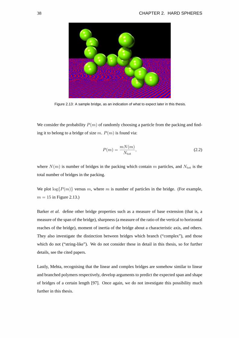
38 CHAPTER 2. HARD SPHERES
Figure 2.13: A sample bridge, as an indication of what to expect later in this thesis.
We consider the probabilityP (m) of randomly choosing a particle from the packing and find-
ing it to belong to a bridge of sizem. P (m) is found via:
P (m) =mN(m)
Ntot, (2.2)
whereN(m) is number of bridges in the packing which containm particles, andNtot is the
total number of bridges in the packing.
We plot log{P (m)} versusm, wherem is number of particles in the bridge. (For example,
m = 15 in Figure 2.13.)
Barkeret al. define other bridge properties such as a measure of base extension (that is, a
measure of the span of the bridge), sharpness (a measure of the ratio of the vertical to horizontal
reaches of the bridge), moment of inertia of the bridge about a characteristic axis, and others.
They also investigate the distinction between bridges which branch (“complex”), and those
which do not (“string-like”). We do not consider these in detail in this thesis, so for further
details, see the cited papers.
Lastly, Mehta, recognising that the linear and complex bridges are somehow similar to linear
and branched polymers respectively, develop arguments to predict the expected span and shape
of bridges of a certain length [97]. Once again, we do not investigate this possibility much
further in this thesis.

2.4. INTERMEDIATE SYSTEMS 39
2.4 Intermediate Systems
Real systems will often lie between the idealised limits of Sections 2.2 and 2.3. In particular,
“colloidal” systems are almost never truly colloidal. Granular systems are more often indis-
tistinguishable from perfectly athermal systems, but even these often behave as “intermediate”
systems, for example when fluidised.
In this short Section we give some examples of how compromise systems lying in between can
be useful. We begin by defining a measure of where on the spectrum a particular system lies.
2.4.1 Gravitational P eclet Number
The Peclet number is a dimensionless quantity usually used to describe the competition be-
tween viscous and Brownian forces in a flowing colloidal system, for example
Pe ∼ τviscous/τBrownian ∼ γr3µ
kBT
is one definition appropriate to sheared systems, whereγ is an imposed shear rate,µ is the
solvent viscosity, andr the particle radius.
In our sedimenting colloidal systems, we desire a similar quantity, but which compares the
relative timescales associated with sedimenting and Brownian motion. We can do this simply
by comparing energies: Brownian motion occurs with an energy∼ kBT per particles, whilst
a particle sedimenting through a heighth acquires an energymBgh, wheremB is its buoyant
mass, thus
Pegrav ∼ τBrownian/τsed ∼ Es/EB ∼ mBgh
kBT.
Here,h is a representative height which we take to be the colloidal radiusr, and since the
buoyant mass is simplymB = ∆ρV = (ρpart−ρs)V , whereρpart is the density of the particles
andρs is the density of the solvent, we have
Pegrav ∼ 4π∆ρgr4
3kBT.
We can now be more objective about what it means to be thermal or athermal; a system is said
to be truly Brownian ifPegrav ¿ 1. It is athermal ifPegrav À 1. If Pegrav ∼ 1, one most
be a bit more careful. We elaborate in the next Section. Ther4 dependence ofPegrav means
that the behaviour of a particular system can move rapidly from one regime to the other with a
seemingly small change in the particle size.

40 CHAPTER 2. HARD SPHERES
We should note here that this definition of the gravitational Peclet number is essentially the
same as the definition of gravitational length,lg = kBTmBg , which is sometimes used.
2.4.2 Some intermediate colloidal systems
We mention some systems which display what we currently refer to as behaviour intermediate
between Brownian and granular, that is, systems withPegrav ∼ 1. The obvious everyday
example demonstrates how very few systems are truly Brownian, and is simply the barometric
pressure distribution in the atmosphere.
The density profile in the atmosphere, the barometric distribution, is well known to vary as
ρ ∝ ρ0 exp{−α (z−z0)}. Famously, this distribution is the same in colloidal systems, a fact
demonstrated in experiment by Perrin, who observed this so-called sedimentation equilibrium,
thereby contributing to the widespread acceptance of the reality of molecules, and ultimately a
Nobel prize.
This barometric distribution under gravity can actually be quite useful in establishing the phase
behaviour of intermediate systems. The hard sphere phase behaviour described in Section 2.2.1
is a function only of density, and it turns out that ifPegrav is modestly high, then the density
of the bottom of the sediment can exceed the melting volume fractionΦm. If this is so, then
it is possible to observe glasses at the bottom of the sediment followed by equilibrium crystal,
followed by a supernatant fluid phase. This effect is termed the fan [99].
This effect can be exploited to grow crystals on a base (either flat or patterned), provided that
the particles remain small enough thatPegrav < 1 [100, and references therein]. In doing this,
they obtain a sedimented crystal; this sort of research is of interest in, for example, the area
of photonic crystals (colloidal crystals typically have lattice spacings appropriate for working
with visible light).
Despite the usefulness of the above systems, sedimentation is usually a nuisance. In this thesis,
we are interested specifically in whether varying the Peclet number from∼ 10−3, in which
particles crystallise before they sediment, toPegrav ∼ 1 (just greater than, in fact), where
although the fan can be seen, it is greatly compressed, and essentially no crystallisation is seen
in the sediment.
As a last remark on intermediate systems, in addition to the colloidal systems, the vibrated and
shaken granular systems described in Section 2.3 above are in some sense intermediate, since

2.5. BROADER CONTEXT: A JAMMING PHASE DIAGRAM? 41
the particles are excited by the agitation into something arguably akin to Brownian motion.
Under these circumstances there is a balance between gravity and the motions induced by
shaking which result in these granular systems displaying similar properties to the “colloidal”
systems described above. In this sense they are also seemingly intermediate systems. This has
been addressed explicitly (see for example [101]); this comment leads us neatly to a discussion
of whether these parallels reflect deeper common underlying physics.
2.5 Broader Context: A Jamming Phase Diagram?
We have described both thermal and athermal systems. Both arguably show examples of un-
expected structural arrest. Athermal systems are forced by gravity into arrested states; pictures
such as that of Cates and co-workers [9] involving force chains can clearly be described as
jammed. There can be little doubt that, although the microscopic details are elusive, athermal
systems are arrested by an applied stress. Although it is not so obvious that thermal systems
can be jammed in the same sense, they can certainly form arrested states, not least of which is
the hard sphere glass.
In an attempt to link structural arrest in these systems, Liu and Nagel introduced the notion of a
generalised jamming phase diagram [102, 103]. They envisage both the jamming transition and
the glass transition as being examples of limits of a generic non-equilibrium fluid-solid transi-
tion. Little evidence has really emerged to support this appealing idea; one investigation has
studied such transitions in attractive colloidal systems by adjusting density, attraction strength
and applied stress, and in each case concluded that they showed the same basic solid-like be-
haviour (such as for example in the elastic modulus) [104].
Whilst it is still debatable whether these types of transition are really related (and consequently
whether the term “jammed” ought to be used to refer to arrested states which are not subject
to an applied stress [105]), it does seem a reasonable proposition. It raises a huge number of
questions, [102], but the important point for us is that it also raises the possibility that arrest
under imposed stress and the glass transition are different aspects of the same phenomenon.

42 CHAPTER 2. HARD SPHERES
2.6 Summary and Motivation
We have discussed generic properties of packings of spheres. We have seen how thermal hard
sphere systems can display remarkable properties, including a glass transition. We have also
seen how these systems behave when subject to an overwhelming uniaxial force.
Following this, we have discussed systems intermediate between the two. We avoided, how-
ever, a definition of the point at which a system makes the transition between these states; this
is necessarily ill-defined. Presumably, there exists some point on the gravitional Peclet number
spectrum at which a system will display properties of both.
It has been suggested that an applied stress can cause jamming. Moreover, it has been suggested
that such an applied stress may be responsible for the glass transition. As Kegel says [74]:
The important question that remains is if packings can be identified that are
present under normal gravity but not under low gravity and vice versa. This
question may hopefully be answered by further work using confocal mi-
croscopy and an appropriate model system.
This is the underlying theme of this thesis, and the central aim is to apply the structural analysis
of Section 2.3.3 to two systems, one truly colloidal, and one intermediate system. We compare
these with the results from simulations of athermal systems, to confirm or deny the presence of
load-bearing structures in these samples.
Section 2.5 discussed the possibility that forcing the system into a non-ergodic state can either
be performed by increasing its density or applying a stress, or a combination of these. By
attempting to find force-bearing structures in glassy samples, we are to some extent attempting
to find a sense in which colloidal glasses can be described as jammed. If we do so, then we
provide evidence in support of a jamming phase diagram.

Chapter 3
Confocal Microscopy of Spherical
Colloids
This Chapter describes the image of a colloidal particle as observed when using a confocal
microscope. The point of describing this process is ultimately to justify the method used for
locating particle centres. This Chapter will discuss the confocal imaging process as a series
of evolutionary steps from the generic imaging process, as well as its inherent limitations. A
reasonably full mathematical description of the resolution of a microscope, in three dimen-
sions, is outlined. This will explain how confocal point scanning microscopes can deliver an
improvement in resolution over conventional microscopes. Finally, we derive a model for the
confocal microscopy image of a colloidal particle, and compare this with our observations.
3.1 Image formation
3.1.1 The Imaging Process
To begin, we consider the generic observation system. Despite its familiarity, the simple act
of looking at an object is not trivial. The imaging process that we employ in doing this is a
particular implementation of the generic imaging process illustrated in Figure 3.1.
Figure 3.1 illustrates the three requirements of any imaging system. The object,o(x, y, z),
represents the visible electromagnetic radiation emanating from a real object, and is in general
three-dimensional. The image isf(x, y), and is here shown to be two-dimensional. The op-
eration that forms one from the other is performed by the imaging system, and is represented
43

44 CHAPTER 3. CONFOCAL MICROSCOPY OF SPHERICAL COLLOIDS
Object plane Image plane
Object
Illumination
Detector
Optical axisσ σ
Imagingsystem
o(x,y,z) f(x,y)T[]DESIGNATION:
Figure 3.1: The generic imaging process, comprising a radiating object o(x, y, z), an imaging system,T [ ], and the detected image, f(x′, y′).
by T [ ]. In the case of a human eye, the imaging operationT [ ] is performed by the lens and
f(x, y) is the image cast on the retina.
We now demonstrate that the imaging processT [] can be written as a convolution process. This
description is vital, since both digital filtering and modelling the image of a spherical colloidal
particle are performed in these terms.
An extended objecto(x, y, z) can be considered as a finely-spaced series of adjacent points (a
grid, or lattice). Each point can be considered a delta function at some arbitrary point(a, b, c):
δ(x−a, y−b, z−c).
Thus the image of the object can be written in the form:
o(i, j, k) =∫ ∫ ∫
o(x, y, z)δ(i−x, j−y, k−z)dxdydz,
for arbitrary position (i,j,k) and where the integrals are over the field of view. This is a null
operation, but permits us to proceed. We have that
f(x′, y′, z′) = T [o(x, y, z)],
so that
f(x′, y′, z′) = T
[∫ ∫ ∫o(x, y, z)δ(x′−x, y′−y, z′−z)dxdydz
].
Provided the imaging operationT [ ] is linear, which we shall always assume, then this relation
reduces to:
f(x′, y′, z′) =∫ ∫ ∫
o(x, y, z)T [δ(x′−x, y′−y, z′−z)]dxdydz. (3.1)
3.1. IMAGE FORMATION 45
We identify from this the distributionT [δ(x′−x, y′−y, z′−z)] as the image of a single point,
which in any real imaging system is not itself a single point; we return to thispoint spread
function later, where we discuss its origin and discover that it is an inherent feature of any
imaging system.
We notice that the expression for the observed intensity,f(x′, y′, z′), is a convolution integral.
f(x′, y′, z′) is therefore the convolution of the system point spread function with the object
illuminance, which will be written more neatly as
f(x′, y′, z′) = T [δ(x′ − x, y′ − y, z′ − z)]¯ o(x, y, z)
in which the symbol “ ” denotes convolution. No distinction is made between the convolution
operator in two- and three-dimensions; the appropriate case will be clear from the context.
The image produced by any imaging system is simply the convolution of the effect that it has
on a single point object with the original image. This is equivalent to the statement that the
imaging system places a copy of the point spread function at each point in the final image,
scaled by the intensity of the object at the corresponding point. This property can be exploited
to perform point-wise image processing operations, such as filtering. It also forms the basis for
one technique for identifying particle locations; we shall consider this later.
3.1.2 Magnification
At this point, it may be anticipated that the purpose of many imaging systems is to perform
magnification, that is, that the extent of the imagef(x′, y′, z′) differs from that ofo(x, y, z).
Although this is often the purpose of a particular imaging system, it is not relevant to this
discussion. Since the ultimate aim of this discussion is only to establish the functional form
of images formed, and is not concerned with scaling factors, unit magnification is assumed
throughout. In practice, magnification is determined by calibration during experimentation.
3.1.3 Aberrations
In this thesis, the imaging systems used are viewed in a simplistic, idealised way. In particular,
aberrations, or imperfections in the imaging components that give rise to imperfections in the
image, are largely neglected. Aberrations are discussed generally in [106], and more mathe-
matically in [107]. In general, as well as familiar conditions such as astigmatism, coma, and
distortion, there are two principle aberrations.

46 CHAPTER 3. CONFOCAL MICROSCOPY OF SPHERICAL COLLOIDS
The first is chromatic aberration, which is a consequence of the different wavelengths (colours,
hence the name) being refracted differently by lenses within the imaging system. Concave and
convex lenses act oppositely in this effect, so can be combined to form anachromatic dou-
blet. It is impossible to correct concurrently for all wavelengths, so some compromise must be
achieved. Abbe, the major name associated with aberrations, chose to correct simultaneously
orange and blue due to their apparent importance to the human eye; this correction became
known as Achromat. Though seemingly still simple, the next level of complexity focuses cor-
rectly orange, green, and blue light. This is the Apochromat standard, and is the most exacting
standard typically used.
The other correction most frequently considered is the curvature of field. Using simple lenses,
the focus field produced is not perfectly flat. Figure 3.2 illustrates this in the case of a single
convex lens. The result of this effect is that if objects visible in the centre of the field of view are
in focus, then any objects in the outer part of the field of view will be out of focus. To correct
for this aberration requires the focus field of the compound lens to be flat. This is performed
by a device known as the field flattener; the appropriate standard here is Plan, which we will
take as sufficiently good without further consideration.
Figure 3.2: Curvature of field
Plan Apochromat (Plan Apo, PA) is the standard used throughout. It is assumed that since the
objectives used here are research grade, they are essentially entirely aberration free. Ultimately
the quantitative methods used in this thesis are validated by calibration; any effects due to
aberrations are not distinguished from the other experimental errors.
For completeness, it is worth noting that the usual statement of an aberration-free imaging
system is thatn sinσ
n′ sinσ′= constant,
where the symbols are as defined in Figure 3.1, and the constant is in fact the magnification,

3.2. RESOLUTION 47
which we disregarded earlier. This is known as Abbe’s sine condition, after its German propo-
nent. The similarity between his name and the effect is coincidental.
It is interesting to note that these technically accomplished corrections are not performed in the
human eye, which remains (optically, at least) a rather straightforward imaging system. Rather
aberration correction must be performed by external means (spectacles or contact lenses for,
for example, astigmatism). There is even some evidence that a degree of aberration correction
is performed “on-the-fly” by the brain [108].
3.2 Resolution
Regardless of its complexity, the resolution of any imaging system is determined by three
factors: the fidelity of the light sensing detector, the imaging system aperture size, and the
degree of coherence of the illuminating light. We consider each of these in turn.
3.2.1 Detector Fidelity: Segmentation and Sampling Theory
All devices which form an image comprise an array of individual detecting elements, each of
which records the light intensity at that particular place. The degree to which any particular
imaging device reproduces faithfully an object is limited by the fidelity of the detecting array.
That is, the image detecting elements,pixels, or pictureelements1, must be sufficiently small
that the image does not suffer frompixelisation (also pixelation), where the image of an
object is visibly degraded by the detecting array being insufficiently fine. This concept of
resolution as limited by detector segmentation has become much more familiar with the advent
of desktop printers and, more recently, digital photography equipment. In the last few years,
low-resolution portable telephone cameras have made highly pixelated images commonplace.
For comparison, the thesis of Mark Elliot [57] provides the following information: the human
eye’s retina consists ofO(108) rods and cones in an areaO(103) mm2, giving a maximum
possible angular resolution of around6× 10−5 radians. This corresponds to a field of view of
about4× 10−5 of the field of view. In contrast, traditional photographic film consists of grains
of silver halide of sizeO(10−3) mm, which with final prints up toO(102) mm across gives a
resolution of around10−5 of the field of view. Typical charge-coupled devices (CCDs) such as
1Note that the designation “pixels” is often reserved for two dimensions; three dimensional “pixels” are oftencalled volume elements, orvoxels. We do not make this distinction here, and call them all pixels.

48 CHAPTER 3. CONFOCAL MICROSCOPY OF SPHERICAL COLLOIDS
those used in digital cameras are now around2500×2000 = 5×106 pixels, for a physical size
of around10 mm square, giving a resolution corresponding to' 5× 10⁻⁴ of the field of view.
We should note that this is still an order of magnitude worse than our estimate of the resolution
of the human eye, and that a10 mm square CCD chip would have to be around25000 pixels
square, or625× 106 pixels, to reproduce the theoretical resolution limit of the human eye.
Sampling Theory
The previous Section revealed that the appropriate resolution must be chosen to reflect the
ultimate use of the sampled image. It is clear that the resolution must be sufficiently high
that pixelation does not occur, but one may presume that there is a practical upper limit on
resolution, beyond which a more finely divided detector array provides little advantage.
This is undoubtedly true, but in fact for any sampled image, there is a maximum sampling rate
beyond which there is strictlyno gain to be had. This fact is enshrined inSampling Theory,
which is widely described. For an accessible introduction, see [109].
Sampling theory was described initially by Swedish-born American physicist Harry Nyquist
in 1928 [110]. It was refined, and then (in 1949) formally proved by the American Claude
Shannon [111]. The central tenet is variously known as Nyquist- or Shannon-sampling, but it
now seems that the consensus isthe Nyquist-Shannon sampling theorem.
This theorem is stated without proof as: ifs(x) is a function having Fourier transform
F [s(x)] = S(f) = 0, for |f | ≥ W,
then it is completely described by a list of values of the function at a series of points spaced by
1/2W . The valuessn = s(n/2W ) are thesamplesof s(x).
From this we can deduce that a signal can be reconstructed from samples provided that there are
2W samples per unit distance. This sampling rate is the Nyquist frequency (or rate). Sampling
at a rate greater than this,oversampling, is fruitless. If the signal is subject to noise or any
other imperfection, typically the data are sampled repeatedly and subsequently averaged. In
this circumstance, oversampling permits the signal form to be obtained without the need for
the sometimes impractical repeat sampling.
In the case of sampled images, the maximum resolution is determined by the wavelength of the
light used, as we shall explore in the next Section. The image can therefore containa priori

3.2. RESOLUTION 49
no information with a spatial frequency greater than a certain maximum. Once we know this
maximal value, the imaging system magnification can be set such that the size that each pixel
represents, thepixel pitch, is approximately one half of the system resolution.
It may be that sampling at less than the Nyquist frequency is satisfactory. Images which will
be used only on the world wide web, for example, may be acceptable and even desirable if dra-
matically undersampled. More significantly, and we shall return to this later, an undersampled
signal may be entirely reconstructed ifadditional informationregarding its form is availablea
priori .
3.2.2 Imaging System Aperture
The resolution of the detector of any imaging system is the most obvious limitation on final
recorded image resolution. However, if an infinitely finely-divided detector array were possi-
ble, there would be in any imaging system a diffraction-limited resolution due to the inevitable
finite aperture size.
Every practical imaging system must have an aperture through which light must pass during
the operationT [ ]. Light is diffracted by the edges of the aperture, according to the usual wave-
phenomena description of light. To appreciate the effect that this will have on the detected
image we must know the form of the diffraction pattern due to the aperture. To establish this,
we must consider the aperture in more detail.
Apertures
Figure 3.1 illustrates that for any practical imaging system having an entrance aperture, there
is a maximum size of cone of light from the object that can enter. This cone has angle2σ, and
is known as the (object side) angular aperture. Correspondingly, there is an image side angular
aperture. In general the medium is different between the object and image sides, which means
that in determining an absolute measure of aperture, we must consider also the media refractive
indices. We define the object side and image sidenumerical apertures, respectively:
A = n sinσ and A′ = n′ sinσ′
The aperture of a compound imaging system (i.e. one comprising many optical components,
such as lenses) is typically limited by one particular component; it is not necessary to identify

50 CHAPTER 3. CONFOCAL MICROSCOPY OF SPHERICAL COLLOIDS
and characterise the position and dimensions of this precisely. Instead, the limiting compo-
nent’s extent will be imaged forward of that point, to give theentrance pupil. Similarly,
components behind it will also form its image, theexit pupil . Thus consideration of any of
these images will reveal the effect of the limiting aperture on the imaging system.
Consider the particular simple case of a circular aperture, whose amplitude transmittance func-
tion (the entrance and exit pupil functionsτP andτ ′P respectively) can be modelled by:
τ ′P = circ(
r′PR′
P
),
where
circ( r
R
)=
1 : r ≤ R
0 : r > R,
andR is the aperture radius.
Consequences of Imaging System Aperture: Point-spread Functions and Diffraction-
Limits
It is clear that the aperture of an imaging system will reduce the amount of light that can pass
through the imaging system, and therefore the overall image brightness. There is another, more
significant, effect. The wave nature of the light passing through the imaging system entrance
pupil results in diffraction. This means that even in a perfectly aberration free imaging system,
the image of a point object is not a point image but a diffraction pattern. Referring to the
notation of Section 3.1.1, we see that this situation corresponds to the case (in two dimensions
for clarity)
f(x′, y′) = T [δ(x, y)] ≡ p(x, y, x′, y′), (3.2)
whereδ(x, y) is a point object at a fixed positionx, y (i.e. here we will not integrate) in the
object plane, andp(x, y, x′, y′) is thepoint spread function (PSF) of the system.
The mathematics of this process in our point scanning confocal microscope are not considered
until Section 3.5, but briefly, in a conventional bright-field microscope Fraunhofer diffraction
gives us that the two dimensional point spread function is described by a function of the form
intensity ∝(
2J1(r′)r′
)2
,

3.2. RESOLUTION 51
wherer′ is the coordinate{x′, y′} in the plane andJ1 is a first order Bessel function of the first
kind (and is the Fourier transform of a circ function.)
This is known as theAiry pattern , and the central lobe theAiry disc . The Airy pattern has
approximately84% of its luminous energy contained within the Airy disc.
We should emphasise that this property is one inherent in all imaging systems. Where the
effects of diffraction are not observed, it is because that image is formed far from the diffraction
limit of the system.
As well as detector segmentation and diffraction-limited resolution, the third generic constraint
on resolution, the coherence of the detected light, has been so far carefully avoided. We con-
sider this briefly next.
3.2.3 Coherence of Illumination
The coherence of the illuminating light is in general important in the microscope, since its abil-
ity to resolve objects is affected by interference. Although the illuminating light used through-
out the experiments described in this thesis was provided by a laser, which is coherent light,
it turns out that we can only ever detect light which is incoherent (since it is fluorescent, see
Appendix 3A). As such, we do not need to discuss coherence further. For the interested reader,
[57] provides a good discussion.
* * *
Resolving two objects
We now discuss what it means to resolve two nearby objects which in general are imaged using
a system suffering from the three effects described above (detector fidelity, imaging system
aperture, and illumination coherence).
Two illuminated points separated by the radius of the Airy disc will have the centre of one
coinciding with the first dark ring of the other. At this point, the points are said to be just
resolvable. This is known as theRayleigh criterion, and whilst somewhat arbitrary, it is the
most common statement of resolution. This defines the resolution limit,ρ, as (remembering
thatA is the numerical aperture,§3.2.2)
ρ = 0.610λ0
A.

52 CHAPTER 3. CONFOCAL MICROSCOPY OF SPHERICAL COLLOIDS
For the purpose of this discussion, the prefactor is not important; as we shall see shortly, it
is different for the confocal microscope. We do note one important figure here, however: the
resolution of all practical microscopes is a large fraction ofλ/A, and sinceλ ' 500nm and
A & 1, the diffraction-limited resolution is typically several hundred nanometers.
3.2.4 The Microscope
The eye is an accomplished imaging device, not least in its tremendous dynamic range. How-
ever, it is limited by its resolution2. Small objects could in principle be imaged at a higher
resolution by bringing them closer to the eye, but despite the eye’s rather impressiveoccular
accommodation, or ability to vary the focal length of its lens by muscular distortion, there is
a limit; in practice even a young healthy eye will be unlikely to manage to image an object as
close as around10 cm. Since the pupil has diameter' 3 mm, this limits the numerical aperture
of the eye to no better than1.5/10 = 0.015. To better this, we need a supplementary imaging
system.
The simplest supplementary device that could be used is the single convex lens illustrated in
Figure 3.3. This is essentially a magnifying glass, or loupe. The familiar pocket magnifying
glass (though seldom expensively manufactured) displays the drawbacks of these devices; that
they are prone to aberration to the extent that only devices up to a magnification of around
10x are realistic. To achieve magnification greater than this, lenses may be used in concert,
Focal Length
Focal Point
Object
Image
Figure 3.3: Image magnification by a single lens.
2The theoretical resolution of the eye is approximately given by Rayleigh’s criterion, which shall be exploredmore fully later:θth = 2ρ =∼ 1.22 λ
D, with the wavelength of visible light beingλ ∼ 500 nm, and the diameter
of the lensD ' 0.8 cm. Thus the theoretical resolution isθth ' 7x10⁻⁵radians. Compare with the reasonableobservation that5 cm high lettering can be observed up to around10 m away, thustan θobs ' θobs = 0.05
10=
5x10⁻³radians.

3.2. RESOLUTION 53
or compounded. Such a device is acompound microscope, with the “micro-” meaning really
only small; in principle this implies objects in the range∼200 nm to1 mm.
The simplest compound microscope involves a two-step magnification: the first lens (theobjec-
tive) produces an image of the object in an intermediate image plane. The second magnifying
lens, theeyepiece, has as its plane of focus the same intermediate image plane, and produces
an image of the object at infinity. This arrangement suffers from the disadvantage that the focus
of the composite device can only be changed by moving both of the lenses together. This is
rather inconvenient, but it is straightforward to avoid by incorporating atube lens, as in the
infinite-tube-length compound microscope.
The Infinite-tube-length Microscope
The infinite-tube-length microscope is illustrated in Figure 3.4. In this configuration, the objec-
tive forms an image at infinity, which the tube lens brings to a focus at the intermediate focal
plane. Once again, the ocular focuses on the intermediate focal plane, thereby imaging the
object. The axial position of the objective has in this situation little effect on the light received
by the tube lens, so that focusing can be achieved by moving only the objective lens. This
microscope requires so-calledinfinity corrected objectives.
The right-hand image in Figure 3.4 shows the illumination as in most research microscopes.
This is, however, only one particular configuration. We now briefly discuss the requirements for
the illumination, since it becomes important when discussing the extension to point scanning
microscopes.
Brief Aside: K ohler Illumination
It is widely accepted [57, 106] that there are three basic requirements for illumination of an
object:
1. Only the area of the object under consideration should be illuminated, to reduce the
possibility of stray reflections.
2. The aperture of the illumination must be adjustable to vary the area of the object being
illuminated, and the degree of coherence of the illuminating light.

54 CHAPTER 3. CONFOCAL MICROSCOPY OF SPHERICAL COLLOIDS
Microscope Exit Pupil
Filament Lamp
Intermediate Image Plane
Object
Condensing Lens
(Condenser) Aperture Stop
(Collector) Field Stop
Collector Lens
Ocular
Tube Lens
Objective
Objective Exit Pupil
RetinaRetina
Figure 3.4: The infinite-tube-length compound microscope, showing the imaging (left) and the illumination(right) sets of focal planes. Note that in the left image, rays behind the objective are parallel. In the other,rays behind the condenser are parallel. (The right-hand image shows a microscope set up for Kohlerillumination, which we shall discuss shortly.)
3. Perhapsmost importantlyhere, the illumination of the object must be of (controllable)
uniform intensity.
These requirements can be met in a variety of ways. The best is as first proposed by Kohler, and
has in front of the object a condensing lens and illumination source, as indicated in Figure 3.4.
To be able to achieve Kohler illumination, a microscope must have an illumination field stop
that may be imaged at the object plane, and the condenser front focal plane must be coincident
with the condenser aperture stop. These conditions are quoted without proof; their effect is
to ensure that this system permits the almost inevitably non-uniform illuminating filament to
be cast at the object plane as a uniform “sheet” of light. This is achieved by the condensing
lens imaging the filament “at infinity”–see the parallel rays exiting the condenser in Figure 3.4
(right). Most modern microscopes are designed to use Kohler illumination; to achieve this in

3.3. IMPROVEMENT IN RESOLUTION USING POINT SCANNING MICROSCOPES55
practice, the following steps are followed:
1. Move the condensing lens close to the object plane using its substage focus.
2. Focus on the object plane using the objective turret focus control. Adjust the
brightness if necessary.
3. Close the field iris sufficiently that it partially obstructs the field of view; this
will require a relatively low power objective lens (say10x or 20x).
4. Use the condenser substage focus to form a sharp image of the field iris. At the
same time, ensure the field iris is concentric with the field of view, by using the
substage adjusting screws.
5. Open the field iris to just past the point where it can no longer be seen; further
than this introduces the possibility of stray reflections. (Exceptionally, one may
wish to view an object that is smaller than the field of view. In this case, open
the field iris sufficiently, but no further.)
6. Observe the lamp filament at the objective exit pupil; whilst doing so, adjust
its position until its image is centred and sharply focussed.
7. Adjust the aperture iris to achieve the necessary numerical aperture; this is
usually slightly smaller than the objective exit pupil.
The procedure for achieving Kohler illumination is indispensible, and should be adopted for ev-
ery use of the brigth-field microscope. As we shall see, in most practical confocal microscopes
it is not useful specifically, but since the microscope must usually be used for bright-field work
preceding confocal imaging, it is almost always appropriate.
3.3 Improvement in Resolution Using Point Scanning Mi-
croscopes
The previous Section outlined the basic idealisedwide-fieldmicroscope. In this Section we
demonstrate that this is not the only possible configuration, and that in fact the resolution can
be improved by using a much reduced field of view. A point scanning microscope can be used
to achieve this.

56 CHAPTER 3. CONFOCAL MICROSCOPY OF SPHERICAL COLLOIDS
Point Scanning Microscopes
Having discussed Kohler illumination, we may discuss the formation of microscope images by
point scanning microscopes; it is tempting and indeed accurate to justify the use of point scan-
ning microscopes as a means of simplifying the microscope. It is easier to design an optical
system to image a small point than it is to image an extended field of view. This is technolog-
ically significant, perhaps, but from the perspective of the physicist, the primary advantage of
the point scanning microscope is that it permits an improvement in image resolution. Figure
3.5 forms the centrepiece of the argument which explains this fact.
Figure 3.5: Evolutionary stages of Point Scanning Microscopes (from [112]). (a) shows a conventionalwide-field microscope. (b) and (c) show different conventional scanning microscopes. (d) shows a con-focal scanning microscope.
Figure 3.5 (a) gives a representation of the conventional wide-field microscope, in which, in
the standard case of Kohler illumination, the object is uniformly illuminated. The objective
lens images the object onto a fixed extended detector. In this case, the condenser cannot play
any major role in resolution; its purpose is in providing an image of the illumination source
at infinity, and any aberrations it produces are unimportant. Its contribution to resolution is in
determining the degree of coherence of the incident light. Primarily, therefore, the resolution
of the system is determined by the point spread function of the objective lens alone.

3.4. THE CONFOCAL MICROSCOPE IN PRACTICE 57
The first step towards a scanning microscope is illustrated in Figure 3.5 (b), in which the il-
lumination is as in (a), but this time a point detector israster scanned, or scanned linewise
through the image as in a cathode ray tube image. This represents no improvement in principle
over the case shown in (a), but may be more practical. Note here that it is still the objective
lens that is primarily responsible for the system resolution.
Figure 3.5 (c) illustrates the circumstance where it is the illumination source that is scanned
but the detector is an extended one, and there we relabel the lenses to illustrate that now the
precedence of the lenses in terms of their effect on resolution has changed. In this case, the
objective lens “probes” the object with a finely focussed (and therefore subject to the point
spread function) light spot. The collector lens now behaves as the condensing lens in (a), and
as such has little effect on the resolution.
Figure 3.5 (d) illustrates the most useful form of the scanning microscope. From the comments
in the previous paragraph, it can be inferred that an increase in resolution could be achieved
if the collector lens could be used to contribute to the resolving power of the imaging system.
The configuration in (d) allows precisely this, by having a concurrently scanned point source
and point detector. In this case, both the objective lens and the collector operate as imaging
lenses, and the effective system point spread function is the product of the two.
The essence of the improvement in resolution derives from an argument discussed by Lukosz
[113], whereby the resolution of an imaging system can be improved at the expense of its field
of view. The field of view can then be recovered by scanning.
The discussion above is not rigorous, but it is correct. We justify these assertions in Section
3.5, but first we discuss how this scanning arrangement is achieved in practice.
3.4 The Confocal Microscope in Practice
We have considered in some depth the principle of image formation in the confocal microscope.
We now describe the confocal microscope as a practical device. First, we consider the confocal
principle in an everyday form, ahead of a more mathematical description in Section 3.5. We
also suggest a similar level of argument to explain the axial elongation which is characteristic
of most microscopes. Lastly, we describe the confocal microscope as a practical device.

58 CHAPTER 3. CONFOCAL MICROSCOPY OF SPHERICAL COLLOIDS
The Confocal Principle
We discuss here what is often described as the confocal principle, and what is certainly the
most useful property of the confocal microscope. Consider Figure 3.6, which is a version of
Figure 3.5 (d), the generic scanning confocal microsope. This image is the simplest possible
Image PlaneObjective Collector
Object Plane
Confocal Aperture
Optic Axis
Figure 3.6: The confocal principle: light originating from within the focal plane (black) is imaged at theimage plane, as in conventional microscope. Light originating outwith the focal plane (red) is not broughtto a focus at the image plane, and appears as blur in a conventional microscope. A confocal aperture inthe image plane ensures only a thin optical sectionis imaged, so that this detrimental effect is eliminatedby the confocal microscope.
representation of the microscope, showing the image of an object. One set of rays shows a point
at the focal plane being imaged. One can see from the other set of rays illustrated that if light
were to emerge from a point in an extended object lying outwith the focal plane, then it would
not be brought to a focus at the detector. This is equivalent to saying that light originating
from outwith the object focal plane will appear in the detected image as out-of-focus blur.
Eliminating this would substantially improve the image.
We can see, both intuitively and rather appealingly, that by inserting an aperture at the detector
as illustrated, we could eliminate any light that did not occur in the focal plane, and conse-
quently improve vastly the detected image. Since the image plane isconjugate with thefocal
plane, we now appreciate the original of theconfocalmicroscope. Of course, the pinhole size
is important; there is much theory describing its optimal size, but in practice this is very much a
compromise between the greater confocal effect of a small pinhole and the reduced light budget
this affords. In fact, due to the difficulty of manufacturing small apertures (indeed in practice
confocal microscopes use a much larger pinhole at a point conjugate with the object plane but
at a higher magnification for this reason), the pinhole size is seldom continuously variable. A
near-match is usually more than satisfactory.
This description is identical to the more formal mathematical one to follow in§3.5, but this
“everyday” explanation is some respects more informative. It explains why the confocal mi-

3.4. THE CONFOCAL MICROSCOPE IN PRACTICE 59
croscope is able to provide finely resolved images from within a bulk sample: thisoptical
sectioning is overwhelmingly the most important benefit of the confocal microscopefor col-
loidal studies.
An everyday explanation of the axial elongation
The confocal principle discussed above is an appealing and for most confocal microscope users
a satisfactory substitute for a fuller understanding of the confocal imaging process. As well as
the sectioning property, the confocal microscope shares with conventional bright-field micro-
scopes the axial elongation of the observed object. This is a generic and well-known diffraction
property [106], which is mathematically well described. However, in the same way as we es-
tablished a more palatable “everyday” understanding of the confocal principle, we discuss one
other way of viewing the origin of the axial elongation.
Figure 3.7 illustrates the argument for the case of the confocal microscope. Interestingly, the
explanation here applies equally to the conventional microscope, but is more readily appreci-
ated for the confocal case, where there is certain optical section thickness. Consider the first in
the sequence of images, which indicates a fluorescent sphere at some arbitrary axial position
in the microscope. Above this is a cartoon of the region near to the focal plane. The dashed
line indicates the focal plane, while the two solid lines indicate the extent of the optical section.
From this we can see that the conventional case can be recovered by having a very large section
thickness.
The first image shows the sphere a considerable distance from the sphere, where here “consid-
erable” means more than one half of the optical section thickness from the focal plane. Since
no part of the sphere is within the optical section, no fluorescence light is detected.
In the second image, the focus has been advanced along the positive direction until the very
lower edge of the optical section has just passed into the sphere. At this point, a very tiny
amount of light has been detected; this is indicated in the plot of intensity to the right of the
sphere.
By the time the focal plane has reached the edge of the sphere, the optical section has entered
significantly into the bulk of the sphere, and has collected light proportional to the area (volume
in three dimensions) which is shaded differently.
The maximum intensity is detected when the optical section contains the greatest proportion

60 CHAPTER 3. CONFOCAL MICROSCOPY OF SPHERICAL COLLOIDS
z
I(z)
z
I(z)
z
I(z)
z
I(z)
1um
optical section thickness
focal planemoveable
2
z
I(z)
3 4
5
1
αI(z) area
Figure 3.7: The axial elongation of a uniformly-fluorescent sphere due to a microscope of finite sectionthickness. Consider this as a sequence of snapshot images taken from a continuous motion of the focalplane in the positive z-direction; the intensity profile so obtained is indicated to the right of the sphere ineach case.
of the sphere; this occurs when the focal plane passes through the centre of the sphere, as
indicated in the fourth diagram.
After this point, for continuing positive focusing, the detected intensity diminishes symmet-
rically as it increased. The detected intensity is therefore symmetrically distributed about the
z-coordinate of the sphere centre. The fifth image shows a point just after the sphere has left
the optical section, whereupon the intensity has returned to zero.
Figure 3.7 (5) therefore shows the intensity profile recorded for a single isolated particle, and
illustrates the point of this discussion: a finite section thickness implies an intensity profile of
greater spatial extent than the original object. In other words, the object is elongated by the
finite section thickness.
It should be emphasised that if this description is at all useful despite its simplicity, it is because

3.4. THE CONFOCAL MICROSCOPE IN PRACTICE 61
we take as given that the system does not have an infinitesimally thin optical section. The
mathematical description of the elongation considers the PSF in terms of diffraction at the
entrance pupil, and, in the confocal case, the confocal aperture. The finite section thickness in
the confocal case works out as a mathematical fact when the rigorous approach is used; with
the same degree of approximation as in accepting the confocal principle, we can accept this as
a reasonable explanation.
The Practical Confocal Microscope
The essential details of the confocal microscope are clearly explained for the general scientist
in the web page of Weeks [114]. This argument is paraphrased here. For more detail, see an
article by Semwogerere and Weeks which expands on this web page [115], or one of a number
of good general references, for example [112, 116].
First, consider Figure 3.8, which shows the basic layout of the conventional (epi-)fluorescence
microscope3. In this diagram, the excitation light enters the microscope and impinges on the
dichromatic or dichroic mirror . This is constructed to have a critical wavelength above which
all incident light is transmitted, and below it is reflected. The particular mirror used in a flu-
orescence microscope is chosen such that excitation light is reflected. The sample fluoresces
and the light returns through the same lens to impinge on the dichroic mirror once more; this
time it is transmitted to the detector.
The usual form of confocal microscope is as shown in Figure 3.9. The illumination source
is typically a laser, to permit the required rather high illumination intensity. This figure also
shows the extension of Figure 3.8 to include the facility to scan the object, to permit a large
field of view. The scanning in this image is by means of a pair of mirrors which are moved
using galvanometers. This is the setup used by the majority of confocal microscopes, but has
the severe disadvantage that it is very slow. A frame rate of about1 frame per second is realistic
for typical colloidal samples at a resolution of around512× 512 pixels.
The physical scanning of the laser beam across the sample is the limiting factor, and al-
though galvanometers are very reliable and reasonably fast (bear in mind that even one typical
512× 512 frame per second requires scanning of512 distinct lines per second, each of which
has512 pixels, meaning adwell time per pixel on the order of microseconds) there are other
3epi- simply means that the illumination is provided via the microscope objective. The alternative is trans-illumination, where the sample is illuminated from the other side.
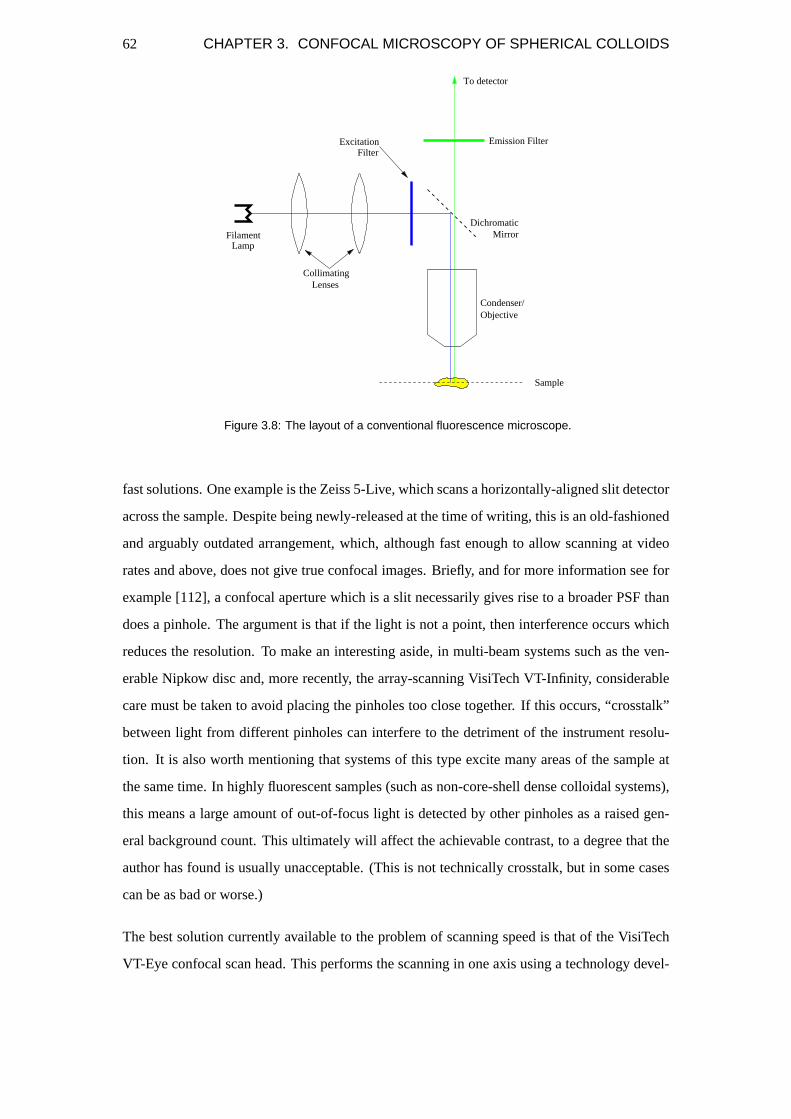
62 CHAPTER 3. CONFOCAL MICROSCOPY OF SPHERICAL COLLOIDS
Condenser/Objective
Excitation
Sample
Emission Filter
DichromaticMirror
Filter
LensesCollimating
FilamentLamp
To detector
Figure 3.8: The layout of a conventional fluorescence microscope.
fast solutions. One example is the Zeiss 5-Live, which scans a horizontally-aligned slit detector
across the sample. Despite being newly-released at the time of writing, this is an old-fashioned
and arguably outdated arrangement, which, although fast enough to allow scanning at video
rates and above, does not give true confocal images. Briefly, and for more information see for
example [112], a confocal aperture which is a slit necessarily gives rise to a broader PSF than
does a pinhole. The argument is that if the light is not a point, then interference occurs which
reduces the resolution. To make an interesting aside, in multi-beam systems such as the ven-
erable Nipkow disc and, more recently, the array-scanning VisiTech VT-Infinity, considerable
care must be taken to avoid placing the pinholes too close together. If this occurs, “crosstalk”
between light from different pinholes can interfere to the detriment of the instrument resolu-
tion. It is also worth mentioning that systems of this type excite many areas of the sample at
the same time. In highly fluorescent samples (such as non-core-shell dense colloidal systems),
this means a large amount of out-of-focus light is detected by other pinholes as a raised gen-
eral background count. This ultimately will affect the achievable contrast, to a degree that the
author has found is usually unacceptable. (This is not technically crosstalk, but in some cases
can be as bad or worse.)
The best solution currently available to the problem of scanning speed is that of the VisiTech
VT-Eye confocal scan head. This performs the scanning in one axis using a technology devel-

3.5. A MATHEMATICAL DESCRIPTION OF THE IMAGING PROCESS 63
Sample
laser
mirrors
x− and y− scanning
dichroicmirror
confocalaperture
microscope
PMT
Figure 3.9: A schematic diagram of the confocal microscope, which extends the conventional fluores-cence microscope to include a pair of scanning devices, a confocal aperture, a laser, and a photomulti-plier tube (PMT).
oped by Noran, known as the Acousto-Optical Deflector (AOD). In this device the scanning in
one axis is performed by sound wave in a crystal which acts as a diffraction grating to deflect
the light passing through it. The details are not important here, but it is inherently a much faster
technique, and permits image acquisition at several hundred frames per second.
Having discussed the practical confocal microscope, we return to developing a description of
the imaging process as appropriate to colloidal particles.
3.5 A Mathematical Description of the Imaging Process
In order to establish the expected form of the image of a spherical particle, we now discuss the
imaging process in more detail. In particular, we must begin by deriving the three-dimensional
Airy pattern which we quoted without proof earlier. We must know this before arguing what
effect it has on the image of a small spherical particle.

64 CHAPTER 3. CONFOCAL MICROSCOPY OF SPHERICAL COLLOIDS
Three-dimensional Airy pattern
The Airy pattern is typically derived in texts on microscopy in some detail in two dimensions
using Fourier optics, and assuming a circular aperture. This is the case cited above. Even
this simple case is complicated [57, 107], and its details not particularly informative for this
argument. Even were we to understand this construction, it would fall some way short of the
three-dimensional diffraction pattern we desire.
Rather, we will outline the arguments given in§8.8 of Born and Wolf [107], and quote only
those results directly relevant to our argument. Once we establish the extensions necessary to
describe confocal microscopy, it will be clear that there is quite sufficient complexity even in
this case.
Here we describe the Airy pattern that represents the point spread function of asingle diffrac-
tion limited lens, from which we can proceed to discuss the effect of combinations of lenses as
outlined in the previous Section.
The argument of Born and Wolf begins by considering a spherical monochromatic wave emerg-
ing from a circular aperture, and converging towards the axial focal pointO. We desire the
disturbanceU(P ) at a point in the neighbourhood ofO. An expression for this can be found
using the Huygens-Fresnel principle, which reduces to (Equation 8.8(12) in [107]) a relation
of the form:
U(P ) ∝∫ 1
0J0(vρ) exp
{−1
2iuρ2
}ρdρ,
whereρ is the radial component of the position vector of a point on the wave-front as it passes
through the aperture fromO, andu andv are the following dimensionless parameters:
u =2π
λ
(a
f
)2
z, v =2π
λ
(a
f
)r
Here,a is the radius of the aperture,f is the separation of the wave-front andO, λ is the
wavelength of the light,z is the usual axial component andr is the position vector of pointP
relative toO (that is, the coordinate in the focal plane).
Thus we see thatu is a coordinate in the axial direction, andv is a coordinate in the focal plane.
To proceed, we write the integral as a sum of a real and an imaginary part:
2∫ 1
0J0(vρ) exp
{−1
2iuρ2
}ρdρ = C(u, v)− iS(u, v),

3.5. A MATHEMATICAL DESCRIPTION OF THE IMAGING PROCESS 65
in which
C(u, v) = 2∫ 1
0J0(vρ) cos(
12uρ2)ρdρ
S(u, v) = 2∫ 1
0J0(vρ) sin(
12uρ2)ρdρ
Lommel [117] introduced the following functions, theLommel functions, to evaluate the
above integrals:
Un(u, v) =∞∑
s=0
(−1)s(u
v
)n+2sJn+2s(v)
Vn(u, v) =∞∑
s=0
(−1)s(v
u
)n+2sJn+2s(v)
Some rather unpleasant manipulation, for which see [107], brings the following two equivalent
expressions for the intensityI = |U |2 in the vicinity of the focus:
I(u, v) =(
2u
)2 [U2
1 (u, v) + U22 (u, v)
]I0 (3.3)
and
I(u, v) =(
2u
)2 [1 + V 2
0 (u, v) + V 21 (u, v)− 2V0(u, v) cos
{12
(u +
v2
u
)}(3.4)
−2V1(u, v) sin{
12
(u +
v2
u
)}]I0,
where
I0 =(
πa2A
λf2
)
is the overall intensity scaling, in terms of variables already defined and the amplitude (≡ A/f )
of the incident wavefront as it passes through the aperture.
The definitions of the Lommel functions give us the following important symmetry properties:
U1(−u, v) = −U1(u, v)
U2(−u, v) = U2(u, v)
V0(−u, v) = V0(u, v)
V1(−u, v) = −V0(u, v)
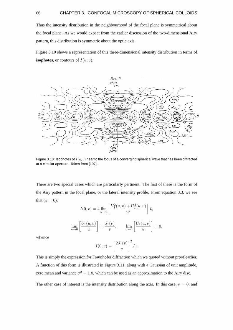
66 CHAPTER 3. CONFOCAL MICROSCOPY OF SPHERICAL COLLOIDS
Thus the intensity distribution in the neighbourhood of the focal plane is symmetrical about
the focal plane. As we would expect from the earlier discussion of the two-dimensional Airy
pattern, this distribution is symmetric about the optic axis.
Figure 3.10 shows a representation of this three-dimensional intensity distribution in terms of
isophotes, or contours ofI(u, v).
Figure 3.10: Isophotes of I(u, v) near to the focus of a converging spherical wave that has been diffractedat a circular aperture. Taken from [107].
There are two special cases which are particularly pertinent. The first of these is the form of
the Airy pattern in the focal plane, or the lateral intensity profile. From equation 3.3, we see
that (u = 0):
I(0, v) = 4 limu→0
[U2
1 (u, v) + U22 (u, v)
u2
]I0
limu→0
[U1(u, v)
u
]=
J1(v)v
, limu→0
[U2(u, v)
u
]= 0,
whence
I(0, v) =[2J1(v)
v
]2
I0.
This is simply the expression for Fraunhofer diffraction which we quoted without proof earlier.
A function of this form is illustrated in Figure 3.11, along with a Gaussian of unit amplitude,
zero mean and varianceσ2 = 1.8, which can be used as an approximation to the Airy disc.
The other case of interest is the intensity distribution along the axis. In this case,v = 0, and

3.5. A MATHEMATICAL DESCRIPTION OF THE IMAGING PROCESS 67
Figure 3.11: (left) A plot illustrating the form of the Airy pattern in the focal plane, which varies as[
2J1(x)x
]2
(see text), and a zero-mean, unit amplitude Gaussian of variance σ2 = 1.8 which approximates thecentral peak well. (right) A plot illustrating the form of the Airy pattern along the axial direction in the
neighbourhood of the focal plane, which varies as(
sin u/4u/4
)2
(see text). Also shown is a similar Gaussian
of variance σ2 = 1.4.
the twoVn functions in expression 3.4 reduce to
V0(u, 0) = 1, V1(u, 0) = 0.
This gives us that
I(u, 0) =4u2
[2− 2 cos
12u
]I0 =
(sinu/4
u/4
)2
I0.
These diagrams, in Figure 3.11, illustrate the sole point of the description of the microscope
imaging system and its point spread function. We have the crucial properties that the point
spread function of a diffraction-limited imaging system with a circular entrance pupil is
• symmetric, both in the focal plane about thez axis, and about the focal plane
• well-modelled up to the first minimum in both the lateral and axial directions by a Gaus-
sian.
These properties allow us to perform particle location. The above discussion has concerned
imaging performed by a single lens, but these properties remain appropriate in a confocal
microscope, when imaging is performed by more than one lens. We now consider the extension
to confocal microscopes.

68 CHAPTER 3. CONFOCAL MICROSCOPY OF SPHERICAL COLLOIDS
Extension to the Confocal Microscope Case
The preceding discussion explained the process of image formation using a single lens point
spread function. As we discussed in Section 3.3, the configuration of a confocal point scanning
microscope takes advantage of the resolving power of each lens in the imaging system.
From here we can straightforwardly deduce the form of the point spread function of the con-
focal point scanning microscope. The confocal system has an overall point spread function
which is the product of the point spread functions of the two lenses.
Since in our case we always use identical lenses for the objective and collector, if
I(0, v) =(
2J1(v)v
)2
is the functional form of the point spread function in the focal plane (u = 0), then in the
confocal case
Iconfocal(0, v) =(
2J1(v)v
)4
Similarly, the equivalent expression for the axial variation
I(u, 0) =(
sin(u/4)u/4
)2
becomes
Iconfocal(u, 0) =(
sin(u/4)u/4
)4
.
Figure 3.12 (left) shows the lateral improvement in the resolution by using a confocal mi-
croscope. This also illustrates that the square of the point spread function is reasonably well
modelled by a Gaussian (in this case of variance0.95). Figure 3.12 (right) illustrates the same
point for the axial resolution. There the variance is0.7. That the point spread function in the
confocal case is approximately Gaussian is entirely unsurprising given the information that that
in the conventional case is too, since the square of a Gaussian is itself a Gaussian.
The understanding of the PSF to this point very nearly sufficient to adequately explain the
observed intensity profile through a fluorescent colloidal sphere. There is a further subtlety
which ought to be outlined.

3.5. A MATHEMATICAL DESCRIPTION OF THE IMAGING PROCESS 69
Figure 3.12: The improvement in resolution due to a confocal microscope in the lateral direction (left)and the axial one (right). In both cases, the dashed line shows the form of the point spread function inthe conventional case, and one of the solid lines is the confocal case. Also shown as a solid line in eachcase is a Gaussian approximation (but not fit)–the variance of the left is 0.95, and that of the right is 0.7.The Gaussian approximation is a very good approximation to the confocal case.
Fluorescence Confocal Microscopy
In the preceding argument, it is assumed that the wavelength of the light is constant throughout
the imaging process. This permitted us to use an effective system point spread function which
was the square of the single lens PSF.
In fact, since the emitted fluorescence light is of longer wavelength than the excitation light
(Appendix 3A), the PSF of that lens which operates on the emitted light will be of lesser extent.
(As an aside, this means that scanning microscopes of the form of Figure 3.5 (c) produce higher
resolution images than those of the configuration shown in Figure 3.5 (b); that is, an objective-
scanning microscope is inherently a better fluorescence microscope than is a collector-scanning
one.)
Rather than the pure product of the single lens PSF with itself, the correct form should be
peffective(u, v) = p(u, v)× p(u/β, v/β)
whereβ = λ2/λ1 is the ratio of the fluorescence wavelength to the incident wavelength.
Thus the in-plane intensity variation will be
I(0, v) =[4J1(v)
v.J1(v/β)
v/β
]2
.

70 CHAPTER 3. CONFOCAL MICROSCOPY OF SPHERICAL COLLOIDS
In this work, β ' 530/488 ' 1.1 is not very large, and so this effect is relatively small.
More than this, it will be demonstrated shortly that the most justifiable model of the image of
a spherical fluorescent particle, which is the aim of this discussion, does not require us to take
account of this effect.
3.6 Modelling the Confocal Image of a Spherical Fluores-
cent Particle
At this point, we have an expression for the system PSF, and have shown that it is well-modelled
by a Gaussian in both the lateral and axial directions. The point of this Chapter has been to
establish what the image of a single colloidal particle ought to be, so that we can use this
information in justifying our particle location technique. In this Section we first model the
system PSF using the knowledge gained above, then we use this to produce a model of the
image of a sphere. Finally, we compare this with some measurements to assess how realistic it
is.
3.6.1 A model of the system PSF
In principle, it is possible to model the PSF of an imaging system very carefully and in con-
siderable detail using relevant properties such as the lens numerical aperture and the precise
wavelength. There are commercial software packages which can do this (for example, Huygens
and Autoquant, http://www.svi.nl/products/professional/ and http://www.aqi.com/index.asp re-
spectively). Alternatively, one could measure the response of sub-microscopic (i.e. essentially
“point” objects) many times over and after averaging, recover a convincing system PSF. How-
ever, we argue that since the first peak in the PSF contains overwhelmingly the majority of the
intensity of the distribution, and since we know from the argument above that this central peak
is well modelled by Gaussians, we ought to achieve a good model of the sphere model a good
deal more simply.
To model the system PSF, a simple set of Gaussians of the form
I(x) = I0exp[−1k(x− x0)2]
was generated and placed in a three-dimensional byte array of size21x21x21 pixels. The eight

3.6. MODELLING THE CONFOCAL IMAGE OF A SPHERICAL FLUORESCENT PARTICLE71
bit “byte” data type specified thatA = 255. In practice,
I(x, y, z) = 255exp[− 1k1
[(x− x0)2 + (y − y0)2
]− 1k2
(z−z0)2], (x0, y0, z0) = (10, 10, 10)
allowed the PSF array to be populated in one calculation, and the relative extent of the PSF in
the z-direction to that in the x- and y-directions to be varied.
The pixel pitch is arbitrary; more pixels inevitably give better precision, but the time required
for the convolution operation scales rather badly with kernel size. For this reason, the PSF
array was limited to21 x 21 x 21 pixels. Here the pixel pitch is taken to be100 nm per pixel in
each dimension, which represents a better resolution than is ever used during image capture.
The extent (effectively the variance,σ2 ≡ k2 ) of the PSF was adjusted using the two parameters
k1 andk2, to correspond to reasonable experimental values for the confocal microscope.
A reasonable value for the lateral resolution of the confocal microscope is around200 nm,
and about500 nm in the axial direction. This value for the resolution, as discussed earlier, is
generally taken to be about the point where the Airy function falls to its first minimum. From
Figure 3.12, we see that where this occurs, the Gaussian model has fallen to around5-10% of
its peak value. This assumption allows us to determinek, since
I(x) =I0
10= I0exp[− 1
k1(∆x)]
taking10% as appropriate. Substituting∆x = 2 pixels, corresponding to200 nm, we find that
k1 = − 22
ln 0.1= 1.737, etc.
Similarly in the axial direction,k2 = −52/ ln 0.1 = 10.857.
The model of the PSF is shown in Figure 3.13 (left). Note that the system PSF is an eight bit
image, but the lens PSF is necessarily not, and has been converted to eight bit simply for this
comparison.
3.6.2 A model of the image of a spherical colloidal particle
We now finally turn to the aim of this Section: to obtain an approximation to the fluorescence
confocal image of a spherical particle. The image of any object comprises its “true” image
convolved with the PSF of the imaging system. The first approximation to the “true” image
of a spherical particle is simply a three-dimensional array of bright pixels, as indicated in

72 CHAPTER 3. CONFOCAL MICROSCOPY OF SPHERICAL COLLOIDS
Figure 3.13: Model of the system PSF as a 3d Gaussian surface (left) and the inferred lens PSF (right),whose autoconvolution is the system PSF. As a test of this conjecture, the red curve in the left image isthe autoconvolution of the function shown in the right-hand image. (Only the lateral intensity profile isshown; the axial response is mathematically similar.)
Figure 3.14. This is a100 x 100 x 100 pixel image, with a circular bright region centred on
(50, 50, 50), and with a radius of10 pixels (so corresponding to a real-space distance of0.5
µm). This will be denotedi(x, y, z).
In fact, we are considering the nature of the fluorescence from a PMMA sphere as it is excited
by laser illumination. The scattering of light radiation by a dielectric sphere is more compli-
cated than that implied by an image of uniform intensity, but taking this scattering into account
is vastly beyond the scope of this explanation. Instead, a uniformly intense sphere image will
be assumed.
The final recorded image of the sphere will be referred to as thesphere spread function, or
SSF. The SSF is particular to each modelled sphere, and is defined as the convolution of the
modelled sphere response with the appropriate PSF:
SSFmodel(x, y, z) = i(x, y, z)¯ p(x, y, z)
¯ =
Figure 3.14: Model of a spherical particle (left), the PSF (centre) and the corresponding image (right).

3.6. MODELLING THE CONFOCAL IMAGE OF A SPHERICAL FLUORESCENT PARTICLE73
This first approximation is reasonable; whether it adequately represents the observed SSF for
a sphere of radius0.5µm can only be judged by comparison with experimental data. We note,
however, that it is subtly incorrect as a model of the situation described above. For a brief
explanation of this comment, see Appendix A. We continue with the model described above.
3.6.3 A comparison of the modelled SSFs with real data
All of the above conjecture regarding the observed image of a spherical fluorescent particle is,
though apparently reasonable, not convincing until compared with the image of such a particle
actually observed using the confocal microscope. Since colloidal particles are by definition
never at rest unless externally restrained, it is more difficult than it would at first seem to obtain
a suitable test image. There are two options: the first and most straightforward is to arrange an
arrested state of many particles, in which any particular particle is prevented from moving by
its neighbours. Such a situation may be envisaged in the midst of a dense sediment, but this
is not a suitable solution, since the images of the adjacent particles in general will overlap and
obscure each other’s SSF.
The second and only practical option for measuring the SSF is to use a dilute sample in which
the spherical particles are constrained not to move. These are available commercially, and are
frequently used for calibration. The disadvantage of this method is twofold: firstly, one then
must use whatever spheres are available, and therefore settle for particles that are not composi-
tionally identical to the ones used for experimentation. Secondly, they are not the correct size.
The former is unimportant since it is only the fluorescence in which we are interested, and
there ought not to be any difference between the fluorophores that could have any bearing on
this analysis. The second is more significant; since the SSF is explicitly a function of particle
size, only an inference of the SSF of the actual experimental particles can be achieved.
To obtain real images of spherical particles, one particular set of calibration standard fluo-
rescent spheres was used (TetraSpeck Fluorescent Microsphere Standards Size Kit T-14792,
Molecular Probes, www.probes.com). These particles are available in several sizes, either in
solution, or affixed to microscope slides. As used here, there were six slides available:0.1 µm,
0.2 µm, 0.5 µm, 1.0 µm, and4.0 µm diameter, and one with a mixture of all of these sizes.
These also have the disadvantage that the particles are attached to the coverslip, which may
have an effect on the image of the sphere. We see no significant asymmetry in the image in the
axial direction, suggesting that this is not significant; it is however another potential problem

74 CHAPTER 3. CONFOCAL MICROSCOPY OF SPHERICAL COLLOIDS
with these samples.
Ideally, there would have been a set of spheres of diameter2.0 µm, roughly corresponding to
those used here. Instead, the1 µm spheres were used. Images of these were captured relatively
slowly (50lps), at a pixel pitch of(0.16, 0.16, 0.10) µmpixel−1. The laser power and gain were
very carefully chosen so that the image intensity histogram occupied almost all of the available
dynamic range. In particular, they were chosen to limit the peak value to around the240th grey
level, so that there was certainly no saturation. This is necessary since the simulated SSF has
a rather broad flat peak that could be largely replicated by a sharper peak that suffered from
saturation.
Figure 3.15 shows the modelled intensity profile (solid black line) for slices through the centre
of the sphere in the x-, y-, and z-directions. In this case, the chosen resolution for the lateral di-
rection was300nm, and600nm for the z-direction. It also shows the intensity profile (averaged
over ten spheres) through a1µm diameter TetraSpeck sphere (dashed red line). Obviously, the
profile for the TetraSpeck sphere should be narrower, which it is, but encouragingly the shape
is reasonably similar.
Figure 3.15: A comparison of the modelled intensity profile (solid black line) for a 2µm diameter sphereand the measured equivalent for a 1µm reference sphere. Data are shown for the x-, y-, and z-directions(left, middle, right respectively). The modelled PSF assumes a lateral resolution of 300nm and an axialresolution of 600nm.
In a crude attempt to simulate the intensity profile of a2µm diameter sphere, the distributions
in Figure 3.15 were doubled in size. Figure 3.16 shows the result of this. It is important to note
that this is not the correct way to model this result; doubling the extent of the convolution of
the modelled image with the modelled PSF is not the same as convolving a double modelled
image with the PSF, but the result is nonetheless encouraging. In particular, the lateral extent
are good fits. The TetraSpeck intensity profiles are slightly too broad in x- and y-, but since
they are averages over ten not perfectly enregistered images, this is a very good fit. This
suggests that300nm is a reasonable estimate of the lateral resolution. The axial distribution is

3.6. MODELLING THE CONFOCAL IMAGE OF A SPHERICAL FLUORESCENT PARTICLE75
Figure 3.16: As in Figure 3.15, but this time with the reference sphere artificially doubled in size. Thoughnot wholly justifiable, the agreement is nonetheless convincing.
again reasonably convincing. In this case, it is clearly too narrow to represent the TetraSpeck
spheres. This suggests600nm is an underestimate for the axial resolution. However, these
Figures are based on a very crude model, and we do not read too much into them. The important
conclusions are that the image of a sphere is much broader than the true size of the sphere, and
that the distributions are spherically symmetric.
It is worth mentioning some further points. Firstly, by inspection of Figure 3.13, it is evident
that the PSF model (due to the limited number of pixels used to represent it) is more peaked in
the model that it ought to be. It seems reasonable that this will result in SSFs which are more
sharply peaked that the actual image is. Figure 3.16 does appear to bear this reservation out; the
TetraSpeck images are “flatter” than the model. Furthermore, using a narrower sphere image
to model a1µm diameter sphere would presumably result in a more peaked intensity-profile
still (a smaller image is altered relatively more by the PSF than a larger one). Lastly, we should
emphasise that values for the resolution are approximate figures; the level of agreement shown
in Figure 3.16 is convincing given this.
We make a brief comment here on the assertion of Crocker and Grier that “a typical sphere’s
image is reasonably well modeled [sic] by a Gaussian surface of revolution”. This is certainly
true, as we have seen, for a point particle (the PSF is well modelled by a Gaussian) [118]. It
is not clear that it is true for larger particles; if the model used here holds, then it becomes less
true for larger particles. In reality, the scattering of light from a dielectric sphere is complicated
([119], as cited in [118]) and probably does not give rise to a uniform intensity over the sphere
(unlike the model used here). The resultant sphere image is hard to predict, but I would suggest
that it is not always the case that a Gaussian models particularly well the image of a colloidal
sphere. Even if it does, the success of this model will vary with the size of the spheres. A
Gaussian approximation does account for the important properties quite well (the shape is
76 CHAPTER 3. CONFOCAL MICROSCOPY OF SPHERICAL COLLOIDS
roughly right, and it is at least spherically symmetric). However, we do not recommend a
particle location scheme based on this assertion. It has been pointed out recently that the lobes
can have an important effect at least in two-dimensional conventional brightfield microscopy
[120]; we investigate more fully later.
At this point, we have successfully achieved the aim of this Chapter, in having a arrived at a
convincing description of the image of a spherical particle. We now consider factors which
cause deviation from the ideal sphere image–noise–as well as a note on how the effect of the
PSF could be taken into account.
3.7 Noise in Images
All of the above discussion of image formation in microscopes has assumed that the detector
accurately reproduces the response of the object under study, and in particular that the illumi-
nation is of constant intensity.
In fact, there are many ways in which a detector can fail to reproduce exactly the true image
of the object. These are due tonoise, which is a term used to describe all processes which
affect the image but which do not relate to the object itself. Noise in generic imaging sys-
tems can originate from, for example: the discrete nature of the radiation; varying detector
sensitivity (including photographic film imperfections); unstable illumination; electrical noise;
and transmission errors (including those due to atmospheric variations). These effects can give
rise to different types of noise. One such type is thedata drop-out noise, which is more
familiar as “snow” such as in poor television reception areas. Another is where a composite
detector is formed from smaller detector elements of slightly varying properties. CCDs are a
good example of where this can occur, since they comprise a large number of separate, suppos-
edly identical, detecting elements. Small differences then manifest themselves as a fixed noise
pattern in the image.
3.7.1 Signal-to-Noise Ratio (SNR)
Thesignal-to-noise ratio, or SNR of an image is a means of quantifying the extent to which
noise has degraded it. It is a concept which must be treated with care, since there are differing
definitions. Additionally, it is not clear that a single number is sufficient to adequately describe

3.7. NOISE IN IMAGES 77
the “quality” of an image; it attempts to objectify an inherently subjective concept. This is
particularly so of, say, television images, but is less relevant here where quantitative means are
to be employed. For completeness, we include one standard definition of SNR.
If the detected imagef(i, j) comprises a “signal” part and a “noise” part:
f(i, j) = s(i, j) + n(i, j)
then the respective variances areσ2s = 〈|s(i, j)− 〈s(i, j)〉|2〉 andσ2
n = 〈|n(i, j)|2〉. Signal-to-
noise ratio is simply defined as:
SNR =σs
σn=
√σ2
f
σ2n
− 1,
since the noise in this case is uncorrelated:σ2f = σ2
s + σ2n.
To find the SNR, therefore, we require two ofσn, σs, σf . From one image, we only knowσf .
Occasionally, depending on the image, it is possible to extract a region of constant intensity
(the classic example is a region of sky within a photograph) and inferσn from this. More
generally, and certainly in this thesis, this is not so, and to calculate the SNR, we must obtain
two images (f(i, j) andg(i, j)) of thesame scenes(i, j):
f(i, j) = s(i, j) + n(i, j)
g(i, j) = s(i, j) + m(i, j).
Taking the normalised correlation between the two realisationsf(i, j) andg(i, j):
r =〈(fg − 〈f〉〈g〉)〉
[〈|f − 〈f〉|2〉〈|g − 〈g〉|2]1/2,
which ultimately gives us
r =σ2
s
σ2s + σ2
n
⇒ SNR =√
r
1− r,
permitting direct calculation of the SNR.
Since SNR is somewhat less than definitive, it is not relied upon in this thesis. It has been
found that an experienced eye and some elementary checks (see Chapter5) are satisfactory as
a measure of image quality. In any case, with colloidal samples it is seldom possible to form
two successive images of the identical image, so that the SNR can seldom be calculated for a
genuinely representative sample.

78 CHAPTER 3. CONFOCAL MICROSCOPY OF SPHERICAL COLLOIDS
3.7.2 Dealing with noise in images
In this thesis, it turns out that we deal with noise in a rather particular way. This method is not
the normal means of dealing with single-pixel noise, so we do not discuss very fully the usual
approach to dealing with noise. However, we do discuss the median filter, which is typically
used to deal with single-pixel random noise.
Median Filter
The median filter is extremely straightforward. It deals with single-pixel noise by considering a
region around each pixel in turn. The size of the region is specified by the user, but is typically
3, 5, or 7 pixels. For each pixel, the sampled value is replaced by the median value of all of the
pixels within the region. This has a smoothing effect which tends to reduce the effect of single
pixel noise. Usually, the median filter is applied in two dimensions, so could be applied to each
slice. A three-dimensional median filter would be equally valid.
3.8 Deconvolution of the Point Spread Function
So far we have considered in detail the image of a spherical particle. The original object is,
as described in Section 3.1.1,modified at each point in a fixed and in principle known manner
by the imaging system. We have seen that the image formed is the convolution of the original
object with the point spread function; one may expect that this effect could bedeconvolved
from the image to return the object.
Deconvolution in this way has been implemented, and is often known asinverse filtering [121],
[122]. In principle, deconvolution is actually rather straightforward, using the Convolution
Theorem, in which for two arbitrary functionsf andg:
F{f ¯ g} = F{f} × F{g},
whereF{x} denotes the Fourier Transform of the arbitrary functionx.
For the imagef(x, y, z) formed from the objecto(x, y, z) by the point spread functionp(x, y, z),
f(x, y, z) = o(x, y, z)¯ p(x, y, z),

3.8. DECONVOLUTION OF THE POINT SPREAD FUNCTION 79
so that:
F{f(x, y, z)} = F{o(x, y, z)¯ p(x, y, z)} = F{o(x, y, z)} × F{p(x, y, z)}.
More neatly:
F = OP (3.5)
The Fourier Transform of the original image can therefore be recovered by dividing the Fourier
Transform of the observed image by that of the point spread function:
O =F
P,
and so
o = F−1
{F
P
}. (3.6)
We can therefore recover the original image straightforwardly, in principle. This technique is
widely referred to as deconvolution, and is now applied routinely in commercially available
software packages. However, there is a major drawback. Equation 3.6 shows that there is a
problem whereP goes to zero, since the division will in general become ill-defined. Frequently
any zeroes inP can be identified and carefully neglected without dramatically affecting the
result [122]. In the case of a jinc function (which the lateral PSF is)4, the Fourier Transform
of the PSF (theoptical transfer function, OTF ) is large for low Fourier space frequencies
and falls monotonically to zero at some critical cutoff frequency [121]. As such, the effect of
ignoring where the OTF falls to zero is to neglect the high frequency part in Fourier-space,
which corresponds to low frequency features in real-space. It seems reasonable that such loss
of information at large scale may not necessarily cause significant problems (especially since
a finite field of view has a limited lengthscale). A similar argument also holds in the axial
direction.
The technique of inverse filtering, therefore, can be useful, provided care is taken, in recon-
structing an image given a perfect image and a perfectly well known and reasonably well-
behaved point spread function. There is an important proviso.
Noise and Deconvolution
If the image is subject to noise, the foregoing argument remains relevant, but much more care
must be taken.4A jinc function is simplyJ1(x)
x, by analogy with the sinc functionsin(x)
x.

80 CHAPTER 3. CONFOCAL MICROSCOPY OF SPHERICAL COLLOIDS
In the presence of additive noisen(x, y, z),
f = o¯ p + n(x, y, z),
so equation 3.5 becomes:
F = OP + N .
Applying the same logic once more, we attempt to recover the original image by dividing out
the OTF:F
P= O +
N
P.
Since the noise here is single pixel, or high spatial frequency,N is of large extent in Fourier
space:|N2| ∼ constant. At higher Fourier space frequencies, the noise termN/P dominates
the object term.
This is a fundamental problem in the technique, and particularly serious for noisy images such
as those typically obtained from the confocal microscope. The inverse problem has been the
subject of considerable effort, and there are several schemes for circumventing the difficulties.
For more detail consult standard references ([122], [121]), in particular considering theWeiner
or Optimal Filter (which uses a least-squares approach) and theMaximum Entropy method
(which attempts to find the smoothest image consistent with the data).
Deconvolution is therefore a possible technique, but a satisfactory result from a noisy image is
a demanding challenge, and, it turns out, not necessary for colloidal studies.
* * *
This concludes the description of image formation in a confocal microscope. The above de-
scription was rather mathematical, but it has established the form of the PSF for the confocal
microscope. Moreover, this led to a model of the image of a spherical particle, will form the
basis of the justification of the particle location method which we study in the next Chapter.
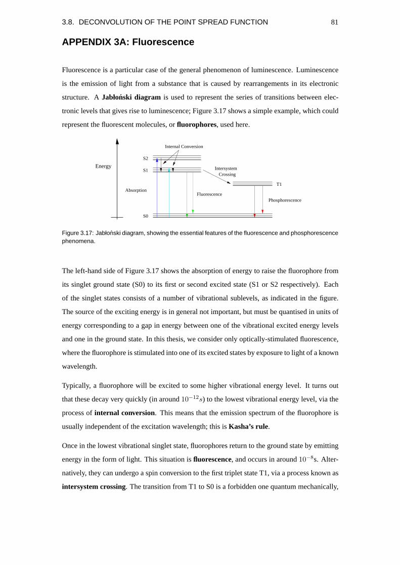
3.8. DECONVOLUTION OF THE POINT SPREAD FUNCTION 81
APPENDIX 3A: Fluorescence
Fluorescence is a particular case of the general phenomenon of luminescence. Luminescence
is the emission of light from a substance that is caused by rearrangements in its electronic
structure. AJabłonski diagram is used to represent the series of transitions between elec-
tronic levels that gives rise to luminescence; Figure 3.17 shows a simple example, which could
represent the fluorescent molecules, orfluorophores, used here.
Absorption
Internal Conversion
FluorescencePhosphorescence
S0
S1
S2
T1
Energy
CrossingIntersystem
Figure 3.17: Jabłonski diagram, showing the essential features of the fluorescence and phosphorescencephenomena.
The left-hand side of Figure 3.17 shows the absorption of energy to raise the fluorophore from
its singlet ground state (S0) to its first or second excited state (S1 or S2 respectively). Each
of the singlet states consists of a number of vibrational sublevels, as indicated in the figure.
The source of the exciting energy is in general not important, but must be quantised in units of
energy corresponding to a gap in energy between one of the vibrational excited energy levels
and one in the ground state. In this thesis, we consider only optically-stimulated fluorescence,
where the fluorophore is stimulated into one of its excited states by exposure to light of a known
wavelength.
Typically, a fluorophore will be excited to some higher vibrational energy level. It turns out
that these decay very quickly (in around10−12s) to the lowest vibrational energy level, via the
process ofinternal conversion. This means that the emission spectrum of the fluorophore is
usually independent of the excitation wavelength; this isKasha’s rule.
Once in the lowest vibrational singlet state, fluorophores return to the ground state by emitting
energy in the form of light. This situation isfluorescence, and occurs in around10−8s. Alter-
natively, they can undergo a spin conversion to the first triplet state T1, via a process known as
intersystem crossing. The transition from T1 to S0 is a forbidden one quantum mechanically,

82 CHAPTER 3. CONFOCAL MICROSCOPY OF SPHERICAL COLLOIDS
but in fact can occur on much longer timescales (10−3 to 100 seconds). This event is therefore
phenomenologically different and is distinguished from fluorescence; it is namedphospho-
rescence. Typically, phosphorescence involves lower energy and therefore longer wavelength
light than fluorescence.
There are three features of fluorescence that are crucial to our understanding of the imaging
process.
Fluorescence is Incoherent
The first follows from what is hinted at above. The fluorescence characteristic timescales given
above are mean quantities as observed following many decay processes. Individual transitions
are governed by randomly-occurring electronic processes, and as such are entirely uncorre-
lated with one another. There is no determinism between the arrival of an exciting photon
and the consequent emission of another. This means that a fluorophore’s emission is entirely
incoherent, regardless of the coherence of the excitation light.
Fluorescence light is Stokes Shifted
The Jabłonski diagram illustrated in Figure 3.17 carefully (if in a cartoon fashion) shows that
the emitted light in each case is of lower wavelength than the incident light. This is schemati-
cally indicated by the colouring in this figure, whereby transitions of lower energy are “redder”
than those of higher energy. This phenomenon isStokes’ Shift, after Stokes’ celebrated obser-
vation of UV-induced (sunlight!) fluorescence from a quinine solution [123].
Fluorescence diminishes in time: Photobleaching
The final property of fluorophores that we must consider isphotobleaching, or fading. We
consider this in no specific detail, except to note that it is an experimental nuisance. The ex-
perimental observation is that the intensity of fluorescence emitted by a fluorophore diminishes
over time. The effect is worsened by higer intensity incident light. The origin of photobleach-
ing is not clear; it may be related to a singlet to long-lived triplet transition as in phospho-
rescence [124], which as well as persisting beyond a useful timescale, is more chemically
reactive. It is claimed [125] that oxygen radicals form as a byproduct of the fluorescence pro-
cess which then react with the fluorophores, thereby destroying their fluorescence properties.

3.8. DECONVOLUTION OF THE POINT SPREAD FUNCTION 83
Regardless of the mechanism, certainly fluorescence is diminished with exposure time. This
is an unavoidable feature of fluorophores: there is considerable effort underway both to find
fluorophores which do not display photobleaching (such as quantum dots), and to diminish the
rate of photobleaching using so-called anti-fade reagents.
Though generally a detrimental effect, photobleaching has found use in the technique ofFluo-
rescence Recovery After Photobleaching(FRAP). FRAP relies on a region of a sample being
bleached extensively by extended exposure to high intensity excitation light. Subsequent obser-
vation of the dark, bleached region within a larger fluorescent one can reveal certain properties.
FRAP has been used to study long time diffusion in colloidal systems, amongst other things
[126].

84 CHAPTER 3. CONFOCAL MICROSCOPY OF SPHERICAL COLLOIDS
Chapter 4
Particle Coordinates from the
Confocal Microscope
This Chapter provides a comprehensive discussion of how to obtain particle coordinates from
the confocal microscope. This begins by describing how best to capture images so that they
contain all of the available information from the samples. We discuss how to deal with the
unavoidable noise in the images, and then outline some possible strategies for obtaining particle
coordinates. To assess the success of particle coordinates, we must describe some tests of
accuracy which we and others have found useful.
We then devote some time to a comprehensive discussion of the most widely-used technique in
confocal microscopy of colloids, namely that of centroiding. Routines which use this technique
were made available to us; we have appraised these and describe their optimal use in some
detail.
A significant result of this work which has not been discussed elsewhere is then described.
We argue that the centroiding procedure as applied can be significantly improved upon, and
develop a method which goes some way to addressing this problem. In doing so, we also
discover that our technique is better suited to dealing with noise in images than the centroid
routines alone.
We reveal that the technique used here is generally useful in improving colloidal particle co-
ordinates which were determined using a centroiding technique. Whilst we discuss how the
technique is itself limited, and in so doing reveal some possible future improvements, it is a
85

86CHAPTER 4. PARTICLE COORDINATES FROM THE CONFOCAL MICROSCOPE
major result of this thesis that the technique is a significant step forward from the publically
available centroiding routines.
4.1 Achieving suitable images
In this Section we discuss how to achieve images in a digital format which are suitable for
subsequent particle location. We first discuss how it is that we can represent light of varying
intensity in a digital format. We then discuss image resolution, specifically how to choose
an appropriate pixel pitch to best balance sufficient fidelity and image size. We then outline
a recipe for capturing good quality images using the confocal microscope, and suggest some
common sources of poor image quality. Lastly, we discuss noise, which is an unfortunate fact
of life even in perfectly captured images.
4.1.1 Digital Representation of Detected Light
The purpose of a light detecting device is to allow the intensity of light originating from a
particular point in the sample to be recorded. In this thesis, the light detecting device is always
a photomultiplier tube (PMT), but it is really only important that the detector delivers a signal
to some recording device, in this case the microscope software, that can be interpreted as an
intensity of light.
In general in digital imaging systems, the (analogue) electrical signal detected is converted to
a (digital) number in the range0-2n−1. The image is then represented by a series of discrete
levels. This representation is therefore both as an image, in which discrete levels,greyscalesor
greylevels, are shown as varying shades of grey, and is amenable to storage by digital medium.
The power,n, is a compromise between fidelity and storage space required. To be visually
pleasing means for gradations between neighbouring greylevels to be barely perceptible, and
requires of order102 greylevels. Conveniently, overwhelmingly the most popular word size has
been8 bits, giving28 = 256 grey levels as the obvious choice, thereby making1 byte per pixel
the de factostandard for monochrome images. Interestingly, “true colour” images comprise
essentially three monochrome primary colour8 bit images which combine to give224 = 16.7
million colour palette. It is said that the human eye can discriminate between' 6–10 million
colours [127, 128, 129], which explains why the true colour standard has not been superseded.

4.1. ACHIEVING SUITABLE IMAGES 87
If the light intensity detector delivers to the software a voltage corresponding to the illuminance
to which it is exposed, then there are two quantities that determine the recorded greylevel. The
first is the illuminance (often loosely thepower) itself; this will fall in a certain range depending
on the specific device (and care must be taken not to damage PMTs by overexposure). The
second is a parameter, thegain, which is usually user-definable and specifies the scaling factor
to be applied to the output signal from the detector. Frequently, there is a second parameter,
the offset, which is simply an additive constant to the signal. Primarily, this is designed to
compensate for a background count.
The above discussion illustrates that there are detector properties that enable the detected image
properties to be altered. To ensure that the image captured contains as much information as
possible, the detector properties must be optimised. Image contrast is the key to fulfilling this
requirement.
Contrast
Contrast can be defined in a number of ways, but it essentially describes the range of intensities
present in an image. In order for an image of a given number of greylevels, ordepth, to retain
as much information as possible, the contrast should represent a large fraction of the available
range of greyscales. One definition of contrast is as follows. At an arbitrary point(x, y) in an
image, the contrast,C(x, y), at this point is:
C(x, y) =I(x, y)− I0
I0,
whereI0 is the image mean background intensity, andI(x, y) is the intensity at(x, y).
To achieve maximum contrast is to use the fulldynamic rangeof the imaging system. That is,
the maximum contrast ought to correspond to the number of available greylevels. The process
of achieving this is aided by use of animage histogram, which is a histogram, or occurrence
count, of intensity values. Figure 4.1 shows a typical image and its histogram, and illustrates
two peaks. This is characteristic of confocal images of colloids captured using the BioRad con-
focal; the higher-valued peak corresponds to the illuminance of the particles, while the lower
one corresponds to noise1. Since this image is of a good sample and was captured by an experi-
enced user, the histogram shows that the image is of an appropriate range of brightness. Figure
1The histogram for BioRad images is curious in having a “noise” peak; this is not present in images of identicalsamples captured using the VisiTech VT-Eye, which provides single peaked distributions.

88CHAPTER 4. PARTICLE COORDINATES FROM THE CONFOCAL MICROSCOPE
4.1 top left and top right simulate the effect of altering the offset (down and up respectively).
Figure 4.1 bottom left and right show the effect of stretching and squashing the range of grey
levels used.
Note that the operations shown in Figure 4.1 werepost processingoperations, that is, were
performed after image capture. In this sense, the effects they purport to illustrate were obtained
by “cheating”. These are known aslookup table (LUT) operations, and are performed here
for illustrative purposes only. This reveals an important point: LUT operations do not increase
the information contained within the images. These areempty operations, and serve only to
increase the visual appeal of the images. To retain the information present in the detected image
the imaging system parameters must be set so that the contrast in the detected
image corresponds to the dynamic rangeat the time of capture.
A histogram is a useful means of ensuring that the appropriate parameters have been chosen.
In particular, it guards against the most likely human error of choosing to capture too high a
mean image intensity, an error which leads tosaturation, where the highest intensity pixels
ought to take a value greater than the image format maximum (usually255) and therefore are
artificially restrained to this maximum value. Figure 4.2 shows a simulation of this situation.

4.1. ACHIEVING SUITABLE IMAGES 89
0 32 64 96 128 160 192 224 256Grey Level
0
200
400
600
800
1000
1200
1400
Num
ber
of O
ccur
renc
es
Reduced Offset
0 32 64 96 128 160 192 224 256Grey Level
0
200
400
600
800
1000
1200
1400
Num
ber
of O
ccur
renc
esOriginal Image Data
0 32 64 96 128 160 192 224 256Grey Level
0
200
400
600
800
1000
1200
1400
Num
ber
of O
ccur
renc
es
Increased Offset
0 32 64 96 128 160 192 224 256Grey Level
0
200
400
600
800
1000
1200
1400
Num
ber
of O
ccur
renc
es
Squashed Range
0 32 64 96 128 160 192 224 256Grey Level
0
200
400
600
800
1000
1200
1400
Num
ber
of O
ccur
renc
es
Original Image Data
0 32 64 96 128 160 192 224 256Grey Level
0
200
400
600
800
1000
1200
1400
Num
ber
of O
ccur
renc
es
Stretched Range
Figure 4.1: Images and corresponding histograms to illustrate the effect of offset (top) and gain (bottom).See text for details.

90CHAPTER 4. PARTICLE COORDINATES FROM THE CONFOCAL MICROSCOPE
0 32 64 96 128 160 192 224 256Grey Level
0
500
1000
1500
2000
2500
3000
Num
ber
of O
ccur
renc
es
Saturated
Figure 4.2: A saturated image and its histogram. In this case, reducing the offset would probably besufficient to rectify the problem adequately; in general both this and the gain will require to be adjusted.
4.1.2 Pixel pitch and image size
As well as ensuring the image uses the full dynamic range of the detector, one must choose an
appropriate region of the sample to study. Unlike a conventional microscope, which usually
has a fixed field of view in which the pixel pitch only be changed with additional lenses (and
some difficulty), in scanning microscopes the user typically has full control over the size of the
region scanned. By altering the angle through which the mirrors (for the sake of argument) are
scanned, a region of varying size can be imaged. Additionally, in confocal systems the user
can typically specify the number of pixels with which to represent the resultant image. The
consequence of this is that it is easy not to appreciate the importance of careful choice of the
pixel pitch. In particular, it is tempting to dramatically oversample the image.
The basic aim when choosing the pixel pitch is to satisfy the Nyquist-Shannon requirement
(see§3.2.1). The resolution of the confocal microscope (§3.6.3) is something in the region of
200-300nm in the lateral direction and500-600nm in the z-direction. These suggest a pixel
pitch of100-150nm and250-300nm in the respective directions.
The particles are isotropic, however, and for the purposes of finding particle locations it is gen-
erally advisable to have the pixel pitch reasonably close to the same value in every direction. (It
is generally easier to locate a reasonably nearly-spherical image, although a small eccentricity
is permissible.) Moreover, it turns out that the particle location schemes we explore in this
Chapter are suited to having a particle of size approximately11-13 pixels in each direction.
For a representative set of particles of diameter2.2µm, this implies a pixel pitch of170-200nm
in each direction.
The ideal pixel pitch is therefore a compromise between these two requirements, but they are

4.1. ACHIEVING SUITABLE IMAGES 91
satisfactorily close. As we argue further in this Chapter, the fact that the particles are of known
shape means we can infer particle locations to greater resolution than the sampling frequency,
suggesting that tending towards the larger of the two is acceptable.
Having determined the pixel pitch, one must then decide upon the desired field of view. This
is determined (for a fixed pixel pitch) purely by the number of pixels in the image, which in
turn is dependent on the image processing hardware. With the computing hardware available
in this enquiry, the practical limit was an image size of around512 × 512 × 100 pixels, for
16 bit images. Doubtless this requirement will be relaxed as desktop computing performance
improves (and particularly memory size increases; the limiting factor in the image processing
on our machines was the availability of memory, which was 512Mb. Even at the time of
writing, this is bordering on obsolete.)
Taking into account the three considerations (the ideal sampling rate, the desire for'11−13
pixels per particle in each direction, and the overall image size), the best compromise in our
systems is something in the region of[0.13, 0.13, 0.2] µmpixel−1 in each direction, giving a
visible volume of' 66µm× 66µm× 20µm, which is large enough for many purposes.
Determining pixel pitch
In order to be able to select a suitable pixel pitch, one must have a reliable means of determining
it. This is achieved using an object of known size, and determining for each optical setup
(that is, which objective lens and scan extent [often controlled using the potentially confusing
zoom]) how many pixels represent that known dimension. In the case of the VisiTech VT-Eye,
the pixel pitch also varies with capture frame rate.
There are a number of standard spherical test beads available for this purpose. For example,
TetraSpeck beads of0.1, 0.2, 0.5, 1.0 and4.0µm diameter are suitable (TetraSpeck Fluorescent
Microspheres Sampler Kit mounted on slides, http://probes.invitrogen.com/, Catalogue No.
T14792). These are versatile, since as well as lateral size calibration they can be used to check
the z-drive precision and to identify spherical aberrations. However, they are rather too small
to give a suitably small error in the pixel pitch. For a4µm diameter particle and typical pitch
of 0.15µm per pixel, so that the particle is around27 pixels in diameter, and assuming an error
in the determination which is no better than±0.5 of one pixel, then the error in the calibration
is around2%.

92CHAPTER 4. PARTICLE COORDINATES FROM THE CONFOCAL MICROSCOPE
A much greater degree of certainty can be achieved by using a Richardson Test Slide. (The one
used here was Reference No. 80112 as ordered from Bio-Microtech Inc, www.bio-microtech.com.
This company appears not to exist now, an alternative supplier is Electron Microscopy Sci-
ences,
http://www.emsdiasum.com/microscopy/products/calibration/richardson.aspx).
These are microscope slides which display a standard test pattern, and which can be used to
identify asphericities in the image, and to provide calibration in both the x- and y-directions.
Figure 4.3 shows a good example of a distorted image which would most likely go unnoticed
without the benefit of a Richardson Test Slide (the “dartboard” pattern ought to be circular).
They are designed for bright-field imaging, but we have found that they provide extremely
bright images in the confocal microscope, under purely reflected light (of course, the emission
filter must be removed to permit this). Using a Richardson Test Slide, distances of order10µm
Figure 4.3: A sample image of a Richardson Test Slide, showing the case of a badly distorted image.Such distortions are surprisingly difficult to see in images of colloidal samples.
can easily be calibrated. From this the pixel pitch can be calculated to considerably better than
1%.
4.1.3 A recipe for capturing good quality images
The following description highlights how to capture good quality images suitable for finding
coordinates.
Once the sample is securely in position, bright-field illumination can be used to find a suit-
able focus in the sample. Bright-field illumination affords a much greater field of view, and
it is therefore much easier to “find” the particles this way. Since there are particles immedi-
ately above the coverslip, these are easiest to find. By bringing the objective lens from a large

4.1. ACHIEVING SUITABLE IMAGES 93
coverslip
z
x
y
laboratory "up"
Figure 4.4: The coordinate system used in this thesis. Note that “up” is down in the laboratory frame.
distance away until it breaks the surface tension of the immersion oil, then applying continu-
ing positive focus very carefully, one achieves most easily an image of those particles at the
coverslip.
At this point, switching to confocal imaging should immediately give an image. Additionally,
there are a number of parameters to set in the confocal case; if any of these are incorrectly set,
no image will be found. This is not true of bright-field imaging, in which case it is known in
advance how to set up the microscope 3.2.4.
By adjusting the laser power and gain roughly to achieve a reasonable image next to the cov-
erslip, the microscope fine focus can be used to image the point where the particlesjust about
disappear; obviously this is subjective, but it is reasonably easy to be consistent in this step.
This position sets the zero of the depth scale.
Since scattering in the sample decreases the signal with depth, the imaging parameters must
be set at the appropriate depth in the sample. Reducing mean intensity means a lower SNR,
so that images captured deeper in the sample are inherently more noisy than shallower ones.
This is unavoidable, and for this reason data should be captured as close to the coverslip as
the phenomenon under observation will allow. To capture three-dimensional images volumes,
the most stringent limitation is that none of the images may show saturation. This means that
the optimum imaging parameters must be set at the shallowest (i.e. the brightest) point of the
region to be imaged. This defines a coordinate system with the z-axis pointing downwards with
respect to the laboratory (Figure 4.4) “up” coordinate (opposite to gravity). The x- and y-axes
are arbitrary and differ between samples.
Another observation which encourages good quality images is that the effect of scattering can
be offset against the effect of photobleaching. By starting to scan deep into the sample, where
the image is of relatively low intensity but not yet photobleached, and proceeding to a shallower
region, then any photobleaching will tend to counteract the natural increase in the intensity.

94CHAPTER 4. PARTICLE COORDINATES FROM THE CONFOCAL MICROSCOPE
(Though the excitation light is reasonably well concentrated in the focal volume, photobleach-
ing is not confined to the focal plane.)
Troubleshooting Image Quality
This subsection is a very quick users’ guide, included in the hope that others may quickly
identify some of the common problems which were encountered during this enquiry.
When images are poor, it is usually because either the particles or the sample mounting are not
very good, or because the imaging parameters have been set poorly. If the particles are poor,
there is little hope beyond imaging more slowly, or, more-or-less equivalently, averaging over
many images. If the sample mounting is poor, changing to a cell similar to those described in
Section 5.3.3 ought to help.
Assuming that the most obvious parameters have been set correctly, that is, that the dichroics
and filters are appropriately chosen, that the laser is operating correctly and at an appropriate
power level, and that the gain and offset are sensible, then it is worth checking some other
possibilities.
Firstly, the confocal pinhole should be set correctly. In some scan heads, this is simply a matter
of choosing the correct size of pinhole. Whilst smaller pinholes give “more confocal” images,
sometimes a larger light budget is useful. The loss of confocality is not always a problem,
particularly when the shape of the particles is known (in which case the loss of resolution
due to the broadened PSF may not be as important as the gain in light collected and therefore
SNR). In some instruments, the size and position of the pinhole can be adjusted; particularly
in the case of the VT-Eye confocal, we have observed drift in these values over successive
experiments.
Secondly, a very common occurrence in longer time colloidal experiments, particularly when
changing between samples, is a poor covering of immersion oil. Though seemingly obvious,
the deterioration of image quality need not be as dramatic as one might expect, and, particularly
in the typically darkened conditions often used, is not always easy to observe.
4.1.4 Noise
Even with the most careful choice of imaging system parameters, we certainly have significant
noise in every image captured. Confocal microscopes are well known for producing very noisy

4.2. DEALING WITH NOISE 95
images. This is largely due to their typically using a photomultiplier tube. Some confocal
microscopes, particularly multi-source systems, use CCD cameras. These have very much
better noise characteristics, but are usually much less sensitive.
To minimise the problem of noise, one can usually employ a degree of averaging. This can
either be in the form of scanning more slowly (increasing the pixel dwell time), or by repeat-
edly imaging the same region. Each has its merits, but both result in a much slower capture
speed. This is important; the capture speed must fast compared with any dynamically processes
being studied is blurring is not to occur; this is frequently a major consideration in colloidal
samples, and usually necessitates a sufficiently fast capture rate that noise is a problem. In our
experience, noise is always sufficiently bad in confocal images that it must be dealt with by
post-processing operations.
4.2 Dealing with noise
The type of noise that confocal images suffer from is usually single-pixel random noise of the
sort that is usually dealt with using a median filter. Previous studies to ours have not done this,
but instead used an approach which we now describe. It is difficult to come up with a defensible
reason for doing this over the median approacha priori, but it turns out that the approach they
have adopted works surprising well and is remarkably robust.
Image Restoration Prior to Feature Location
This section provides a full description of the “Image Restoration” procedure applied to images
before features are found within them. There are two routines, one for two dimensions only
and one fully three-dimensional, both of which we have used as they were written by Crocker
and Grier [118]. This paper describes the principle of operation of the routines. This discussion
is directed towards the three-dimensional version, with two-dimensional examples for clarity.
It should be noted that the following contains a fairly close reproduction of their arguments, as
well as some specific details pertaining to the system in this investigation.

96CHAPTER 4. PARTICLE COORDINATES FROM THE CONFOCAL MICROSCOPE
The Need for Restoration
Any image is liable to be subject to “imperfections” that should ideally be removed. The origin
of particular contributions to such ‘imperfections’ is not explored here, although Crocker and
Grier consider that these may include geometric distortions, non-uniform contrast, and noise.
They note that geometric distortion can be accounted for using standard routines, which are
not described here. The two routines described here were designed to take account of the latter
two imperfections.
4.2.1 Contrast Gradients
The routines were originally applied to images captured by a CCD camera. Such images,
in which different pixels are sampled by different detector elements (of varying sensitivity),
will inevitably display contrast variations. In the case of the confocal microscope, all pixels
are scanned by the same detector, so that this effect should not occur. However, it is still
possible that the illumination will not be uniform across the sample. It seems unlikely that
in this investigation such a correction will be vital, but it appears not to have any undesirable
side-effects, and is a reasonable precaution to take.
Contrast gradients can be dealt with by subtracting this brightness variation. Crocker and Grier
argue that provided the image contains features that are suitably small and sufficiently far apart,
large scale variations in the background can be adequately modelled by a ‘boxcar’ average of
extent2w + 1, wherew is an integer larger than the sphere’s apparent radius in pixels, but
less than the typical intersphere separation. This corresponds to a real-space convolution of the
image with the following kernel:
Aw(x, y, z) =1
(2w + 1)2
w∑
i,j,k=−w
A(x + i, y + j, z + k) (4.1)
The correction for contrast gradients described above relies on the assumption that features
are “small” and “well separated” (“suitably small” and “sufficiently far apart” mean loosely
that the typical intersphere separation is larger than the feature size). For most of the images
considered in this investigation, being typically of samples of volume fractionφ ' 0.5 or
greater, this is not true. However, it appears that the procedure works effectively, as we shall
see. It seems reasonable that the criteria of Crocker and Grier (small and well separated) are

4.2. DEALING WITH NOISE 97
in fact a specific case of a more general sole criterion ‘suitably uniform’, be that mostly low
intensity (in their case) or mostly high intensity (as in this situation, where most of the image
is devoted to particles). This argument appears to hold but for the argument that the “boxcar”
extent must be less than the intersphere separation.
In any case, it has already been noted that this procedure is not of paramount importance in
the analysis of images from the confocal microscope. It should be borne in mind that as well
as the undesirable contrast gradients described above, it is feasible that contrast gradients may
be present in the ‘genuine’ image. This may occur, for example, in an image of a crystalline
sample, in which it is possible that some crystallites may lie in slightly different planes from
others, and one may therefore register a genuine, and correct, difference in intensity from
another. We assume that such effects are negligible.
4.2.2 Noise
While the claim of Crocker and Grier that noise ‘destroys information’ must be regarded with
caution, it is true that removal before features are found is useful. The possible origins of noise
are not discussed here, but it has been assumed, with some justification, that it is ‘single pixel’
noise. This is equivalent to that statement that the noise has correlation lengthλn ' 1 pixel.
Removal of all features having this lengthscale by low pass filtering would certainly eliminate
single pixel noise, but this has the disadvantage of introducing blurring of edges2. Rather, the
usual approach is to convolve with the image the kernel:
Aλn(x, y, z) =1B
w∑
i,j,k=−w
A(x + i, y + j, z + k) exp
(− i2 + j2 + z2
4λ2n
)(4.2)
Since the Fourier Transform of a Gaussian is itself a Gaussian, this attenuates high frequencies
as desired, while more adequately preserving edges.B is the normalisation condition,B =[∑w
i=−w exp(−(i2/4λ2
n))]3
.
2Low-pass filtering, in its simplest form, involves cutting from the Fourier Transform of the image all pointsthat lie above a threshold frequency. Such a circular region in the FT gives rise (upon Fourier transforming oncemore) to a real-space convolution kernel of the formAlowpass = J1(r/w0)
(r/w0), wherer2 = x2 +y2 +z2 andw0 is the
threshold frequency. This kernel effectively places ajinc function, or series of concentric rings, about each pointin the original image, thereby blurring beyond usefulness the processed image.

98CHAPTER 4. PARTICLE COORDINATES FROM THE CONFOCAL MICROSCOPE
4.2.3 Performing the Convolutions
In Principle
If each of the above convolution kernels were applied separately to the the image, the difference
between the two resultant images would represent an approximation to the ideal image. That is,
in principle it is possible to implement equations 4.1 and 4.2 in a single step using the following
(two-dimensional) kernel:
K(i, j) =1
K0
[1B
exp
(− i2 + j2
4λ2n
)− 1
(2w + 1)2
](4.3)
The normalisationK0 = 1/B[∑w
i=−w exp(−(i2/2λ2
n))]2 − (B/(2w + 1)2) is appropriate
for comparison between images filtered with different values ofw, although this will not be
used.
Taking the assumption that the noise is not correlated between pixels,λn is set to unity.
In Practice
In practice, the single step convolution described above is inefficient. A two-dimensional con-
volution requiresO(w2) operations, as opposed toO(w) for a 1d convolution. Above a critical
size forw, therefore, it is more efficient to calculate the convolution kernel in four (six, in
three dimensions) one-dimensional convolutions. Such decomposition is permissible since the
convolution kernelK is circularly or spherically symmetric in two- and three-dimensions re-
spectively. This argument also relies on convolution being a linear operation.
A practical limitation on the convolution is that it involves, for each point(x, y) in the original
images, a sum over all points(i, j) for i = −w . . . w. Clearly, this cannot occur for any point
that lies less thanw pixels from the edge of the original image. This results in a border around
the image, of widthw that must be set to zero. This is the case for those images processed
by the two-dimensional routines which were available. However, in the more recent three-
dimensional version, not only are the convolutions performed in three dimensions, but, prior
to processing, the original image is “padded out” with a border of widthw around the entire
volume. (Above and below the stack, the pixels are all set to the mean intensity value in the
first and last slices respectively. To the sides of the stack, the border around each slice is set
to the average value of the intensity in that slice.) This padding permits the entire image to be

4.2. DEALING WITH NOISE 99
retained following filtering, and is discarded afterwards. It will be shown shortly that the border
retained after the two-dimensional procedure can have interesting effects. We should note that
the averaging used to produce the border is an approximation. In creating a border of any kind,
you are attempting to put in information which you cannot know. It is therefore impossible to
produce an “ideal” border. This is a standard problem in image processing, and the average
described above a perfectly defensible one. It does mean that information derived from this
region is inherently and unavoidably less reliable than from the bulk sample. Since we throw
away particle coordinates from this border region anyway, this is not important in this enquiry.
However, future improvements to particle location should not forget this important observation.
The Convolution Kernels
It is interesting to compare the convolution kernels. To do this, consider the image formation
process as follows:
g(i, j) = f(i, j)¯ h(i, j)
wheref(i, j) is the image to be filtered,h(i, j) is the filter convolution kernel, andg(i, j) is
the filtered image. The convolution theorem then gives us that:
G(u, v) = F (u, v)H(u, v)
whereF (u, v) ≡ F[f(i, j)] is the Fourier Transform off(i, j), etc.
By settingf(i, j) to be a delta function (in practice, for a 512x512 8 bit grayscale image, this
means setting one of the pixels at the centre of the image, say (255,256), to the value 255),
g(i, j) indicates the form of these (two-dimensional) real-space kernels3. That is,g(i, j) =
δ(i, j) ¯ Aλn(i, j). Correspondingly,G(u, v) = F[δ(i, j)]F[Aλn ] = αF[Aλn ], since the
Fourier Transform of a delta function is constant at all frequencies.
Figure 4.5 shows the form of the kernel,Aλn , and its Fourier Transform, while Figure 4.6 does
the same for the ‘boxcar’ smoothing kernel,Aw. It should be noted that for the purposes of
display, each of the Fourier Transforms here actually illustrates theamplitudeof the Fourier
Transform (not the log power spectrum as is often used; this is applied to make best use of the
greyscale range; this was not necessary here). Additionally, the images have all been scaled to
8-bits for clarity. This is not the case during processing.
3This required two 1d convolutions, as described earlier.

100CHAPTER 4. PARTICLE COORDINATES FROM THE CONFOCAL MICROSCOPE
Figure 4.5: The convolution of the noise-suppressing gaussian kernel, Aλn , with the above delta function(left) illustrates its form. The Fourier Transform of this image (right) is, to within a constant (= α in text),the Fourier Transform of the kernel.
Figure 4.6: As above, but this time for the smoothing ‘boxcar’ kernel, Aw.

4.2. DEALING WITH NOISE 101
Figure 4.7: A good quality but noisy image before processing (left). Large-scale contrast gradients arenot significant. Its Fourier Transform is also shown (right).
Figure 4.8: Original image having been filtered using the two-dimensional algorithm (left), and its FourierTransform (right).
A Sample Image
Figure 4.7 illustrates a typical good quality image of a largely crystalline region. This is a slice
extracted from a volume. Firstly this was filtered on its own. The entire volume could then be
filtered using the three-dimensional algorithm, and the same slice extractedfollowing filtering.
Figure 4.8 shows the image after having been filtered in two dimensions. Interestingly, there is
an apparent artefact in the form of a cross-like object running through the centre of the image.
This feature is in fact superimposed on each of the prominent features within the image, and
derives from a convolution in Fourier space with the Fourier Transform of the artefact.

102CHAPTER 4. PARTICLE COORDINATES FROM THE CONFOCAL MICROSCOPE
Figure 4.9: A border of appropriate size (left), and its Fourier Transform (right).
Aside: the artefact
Perhaps unsurprisingly, this artefact is due to the border. Consider the “image” in Figure 4.9,
which simulates a border around a typical image. Its Fourier Transform (Figure 4.9 (right))
shows the artefact is almost trivial.
If r(x, y) is the window, such that:
r(x, y) =
0 : x, y ∈ border
1 : otherwise
that is,r(x, y) is a window that removes anything in the image that lies within the border, then
the final image is:
g′(i, j) = [f(i, j)¯ (Aλn −Aw)] r(x, y)
so that
G′(u, v) =[F (u, v)F[(Aλn −Aw)]
]¯ R(u, v) = G(u, v)¯ R(u, v)
That is, the (FT of the) actual final image is the (FT of the) expected image (the first term on
the right hand side) convolved with the Fourier Transform of the “window”.
Figure 4.10 shows the result of filtering the entire image at once using the three-dimensional
routine (this is the same slice as before). In this case, it is clear that there is no artefact.
We should also observe that even in Figure 4.10 (right), which has no border, there are still some
streaks evident. These are in fact much less pronounced than in Figure 4.8 (right), as both were

4.3. STRATEGIES FOR FINDING PARTICLE CENTRES 103
Figure 4.10: The original image having been filtered using the three-dimensional algorithm (left), and itsFourier Transform (right).
scaled to8-bit images and the central peak in the former is much less bright compared with the
rest of the image; this is clear from the greater number of orders which can be seen in Figure
4.10 (right). These streaks are of unknown origin, but one possibility is that effect of the pixels
on the sampling of the image. The pixels are themselves square, so could be expected to place
a copy of something similar to the artefact at each bright point in the image, much as did the
border. Since the pixels are much smaller than the border in real space, they give rise to a broad
feature in Fourier space. For an indication of what the superimposed streak may look like, see
Figure 4.6 (right), which is a square of size∼ 10 pixels. The streak evident in Figure 4.10
(right) is sufficiently similar to this that this explanation is believable. We do not consider it
further here.
4.3 Strategies for finding particle centres
With the knowledge developed so far in this chapter, it should be possible to determine the
location of the centre of a colloidal particle from its confocal microscopy image. This Section
describes the strategies which can be applied to find particle centres. These are split into
two basic concepts. The first involves identifying particles and then inspecting each in turn
(“finding local maxima and refining”). The second is a more general technique which involves
a deconvolution technique to extract instances of the particle image.
The crux of our being able to identify particle centres is the following:we are able to identify
the centre of a particle from it’s image only by relying on the knowledge of its shape. We

104CHAPTER 4. PARTICLE COORDINATES FROM THE CONFOCAL MICROSCOPE
know that each particle is spherical, and, following the arguments above, we therefore know
the shape of the fluorescence intensity profile through each particle’s image4. (This argument
is weakened, albeit slightly, by the presence of noise.) The focus of this Section is the degree
to which we exploit this knowledge.
This brings us to the most important point pertaining to particle location.
Our a priori knowledge of the particles’ shapes permits location of the par-
ticles to higher precision than the sampling rate. Thissub-pixel resolution
ultimately allows location of particles to substantiallybetter than the resolu-
tion of the microscope.
In principle there is no limit on this statement, though inherent experimental error and limita-
tions in the interpolation techniques used ensure a maximum resolution which cannot be known
in advance.
We consider two routes to identifying particle locations. The first is extremely widely used,
but can only be useful when finding the centres of solidly-fluorescent spheres. The second, a
deconvolution method, is more general, but not used here.
4.3.1 Identify Local Brightness Maxima and Refine
The vast majority of particle location schemes operate on the assumption that the image of a
particle has a maximum intensity at, or near to, its centre. This is certainly so for a perfect
uniformly fluorescent sphere that is perfectly enregistered with the detector. Identifying in
an image the brightest pixels within a region corresponding to the particle size will therefore
give the particle centres. That isthere is a one-to-one correspondence between local bright-
ness maxima and particle centres. (“Local” is important since the image brightness can in
general vary dramatically on the scale of several particle diameters without compromising the
technique.) In practice, the sampling grid will never coincide with the sphere centres. Other
imperfections such as inadequacies in the method used for dealing with noise could in principle
be relevant. Once the local brightness maxima are known, we infer particle locations using a
refinement step. There is a hierarchy of possible refinements, based on the extent to which the
a priori knowledge is relied upon.4Use of a priori knowledge in this way is known asBayesian inference, and is widely used in many fields
[130, 131]. Even the simplest particle location scheme infers coordinates by taking advantage of this informationand is therefore in this sense Bayesian.

4.3. STRATEGIES FOR FINDING PARTICLE CENTRES 105
We emphasise here that prior to refinement we assume we have nearest pixel accuracy. The
refinement step then gives subpixel resolution.
Refinement Using Spherical Symmetry: Centroiding
The simplest, most obvious, technique relies only on the knowledge that the image of the
sphere, the sphere spread function, is spherically symmetric. We consider this in more detail
than the other possibilities since not only is by far the most widely-used technique [132], it
is the method used in all of the papers by both the groups of Weeks and Weitz (for example,
[77, 78, 79])
We describe in some detail the centroid technique shortly (Section 4.5) since it recovers particle
locations satisfactorily even in the relevant dense suspensions. However, it is worth considering
more sophisticated techniques since these can provide a more accurate determination where the
centroid technique fails.
Refinement Using Known Functional Form
Whilst a centroid-based approach appears to work well, it does not make best use of the avail-
able information. In particular, since the extent of the SSF is larger than the particle itself,
when two particles come within a certain distance of one another (the distance is specified
by the imaging system PSF, and is not in general isotropic), the SSFs overlap. This causes
significant difficulties, which we discuss further in Section 4.6.
We anticipate that rather than using a centroiding approach, it would be better to make use of
the knowledge of the SSF functional form, since SSF overlap would then represent a simple
superposition to which a fit could be applied. We could in principle develop an approximation
to the functional form of the intensity profile. Even a simple model may be better than the naıve
centroid (although we should point out the centroiding technique has proved to give reasonable
results for a wide range of systems).
In related systems such as PIV, as well as then-point centroid estimators, there are two other re-
finement estimators which are widely used to approximate the functional form of the observed
intensity profiles. The first is a parabolic peak fit, which assumes a functional form:
f(x) = Ax2 + Bx + C

106CHAPTER 4. PARTICLE COORDINATES FROM THE CONFOCAL MICROSCOPE
From this, it follows (with some non-trivial algebra) that the positions of the particle implied
by this model are:
x0 = i +I(i−1,j,k) − I(i+1,j,k)
2I(i−1,j,k) − 4I(i,j,k) + 2I(i+1,j,k)
y0 = j +I(i,j−1,k) − I(i,j+1,k)
2I(i,j−1,k) − 4I(i,j,k) + 2I(i,j+1,k)
z0 = k +I(i,j,k−1) − I(i,j,k+1)
2I(i,j,k−1) − 4I(i,j,k) + 2I(i,j,k+1).
In these relations,(x0, y0, z0) is the “true” position of the particle centre corresponding to the
candidate (integer) location(i, j, k), andI(i′, j′, k′) is the intensity of the sampled image at
arbitrary position(i′, j′, k′).
In this thesis, there is no basis for using a parabolic fit. There is marginally more for using
a Gaussian fit, however, since Crocker and Grier claim that, at least in two dimensions, the
“typical” image of a spherical particle is “reasonably well modeled [sic] by a Gaussian surface
of revolution”. Section 3.6.3 finds no basis for this assertion (which they do not even attempt
to justify), and the measurements presented there suggest that this is not an accurate remark.
Nonetheless, the simplest Gaussian fit, based on a three-point estimator, is compared with the
centroid approach in the next chapter.
The simple Gaussian fit assumes a functional form:
f(x) = C exp[−(x0−x)2
k
],
but clearly this means that
ln f(x) ∝ −(x0−x)2,
so that the three-point Gaussian estimate is simply parabolic in the natural logarithm of the
sampled pointsI(i, j, k):
x0 = i +ln I(i−1,j,k) − ln I(i+1,j,k)
2 ln I(i−1,j,k) − 4 ln I(i,j,k) + 2 ln I(i+1,j,k)
y0 = j +ln I(i,j−1,k) − ln I(i,j+1,k)
2 ln I(i,j−1,k) − 4 ln I(i,j,k) + 2 ln I(i,j+1,k)
z0 = k +ln I(i,j,k−1) − ln I(i,j,k+1)
2 ln I(i,j,k−1) − 4 ln I(i,j,k) + 2 ln I(i,j,k+1).

4.3. STRATEGIES FOR FINDING PARTICLE CENTRES 107
These two three-point estimators are convenient and widely applied. They rely on the image
of the particle being around three pixels in diameter [132], which may not permit the desired
sampling rate: remembering Section 4.1.2, the pixel pitch ought to be around0.2µm, so a
typical colloidal particle suitable for confocal microscopy (diameter' 2µm) need be at least10
pixels in diameter. Of course, it is extremely important that it is appreciated that this sampling
criterion applies when one wishes to sample anunknownsignal up to a known frequency. In
this thesis, the additional information regarding the functional form of the particle image may
in principle allow recovery of the particle location despite the apparent undersampling. It is not
possible in principle to resolve this conflict, and opinions, judging by the literature [133, 134],
differ on exactly what is the appropriate choice. Bearing in mind, however, that the image is
subject to noise which complicates the choice, and that the validation procedure (4.5) concerns
the so-called Nyquist–Shannon sampling, everywhere in this thesis the particle image will be
in the region of10 pixels in diameter.
This does not, of course, render any less relevant the general technique of fitting to a functional
form. In the Gaussian case, for example, a least-squares fit to a10–pixel cubed volume is
perfectly straightforward, as indeed would be any other (most likely more justifiable) functional
form. As an intermediate measure, the three-point estimator could be applied to the pixels
adjacent to the candidate centre. This compromise is compared in the next Chapter with the
centroiding technique.
The professed advantage of fitting to a functional form was that it would outperform the cen-
troid approach when the SSFs of neighbouring spheres overlap; ironically, this section has
avoided detailing how that could be done. It is well documented and readily appreciated that
the above fits are appropriate only for well-resolved correlation peaks [132, 135]. No attempt
has been made to make any progress in this direction. In addition, since the functional form
is not in general known, a practically better approach would be to fit the measured SSF to the
image.
Refinement Using Measured SSF
This approach would also be algorithmically difficult, but at least the SSF can be measured.
In this case, one would measure the SSF in a window of appropriate size (just larger than the
SSF itself), and attempt to least-squares fit “stamps” of the SSF around the candidate particle
locations.

108CHAPTER 4. PARTICLE COORDINATES FROM THE CONFOCAL MICROSCOPE
This approach would almost certainly outperform the analytical functional form fitting, since
providing the SSF were sampled appropriately, it would take account of aberrations and imper-
fections, as well as accounting more accurately for the system PSF.
This technique is explored much more fully in Section 4.7, where it is proved to be a significant
improvement. However, even this in principle is not the ultimate development.
If we know the SSF, then extracting occurences of this motif must be possible; the way of doing
this involves a deconvolution operation, in much the same way as it is in principle possible to
deconvolve the PSF (§3.8).
4.3.2 Particle Location by Deconvolution of the SSF
We have established that the imaging system can be represented as a convolution process
(§3.1.1), and that we could in principle recover the original form of an imaged object by de-
convolution of the PSF from the observed image. While this was not attempted, that discussion
allows us to detail a similar process by which we could obtain the position of a particle. This
section is therefore merely an interesting aside.
We argued that the imaging system placed a copy of the PSF at each bright point in the original
image. In a similar way, we may consider the image of a particle to be formed by placing a
copy of the SSF at the appropriate place, that is, at the particle coordinate. Mathematically, this
is the convolution of the SSF with a Dirac delta function, so that, for example:
f(x′, y′, z′) = δ(r)¯ s, (4.4)
wheres is the sphere spread function that corresponds to a sphere centred on the origin (thereby
defining implicitly an origin).
By the convolution theorem, we can write this as
F (u, v, w) = F{δ(r)} × S,
whereF (u, v, w) is the Fourier Transform of the imagef(x′, y′, z′), S is that of the SSF and
F{δ(r)} is that of a delta function at positionr. Since the Fourier transform of a delta function
centred on the origin is simply a constant (= 1√
2π or 1, depending on the particular version
of the Fourier Transform definition chosen),F{δ(r)} ≡ α, we find that:
F = αS ⇒ α =F
S⇒ δ(x, y, z) = F−1
{F
S
},

4.3. STRATEGIES FOR FINDING PARTICLE CENTRES 109
whereF−1{} denotes the reverse Fourier Transform.
The situation is complicated slightly in the case where there is more than one sphere in the
image, since in this case it is not possible to define the centres of both spheres as being at the
origin. The Fourier Transform of a delta function which is not centred on the origin is:
F{δ(r−r0)}(k) =∫ ∞
r=−∞δ(r−r0)e−2πik.rdr = e−2πik.r0 .
Thus the Fourier Transform is no longer constant, but contains phase information depending
on its distance from the origin.
This is, of course, the mathematical reason why the convolution process is capable of returning
the locations of more than one particle. If this property did not hold (i.e. there were no phase in-
formation in the transformed delta function) then it would not be possible on back-transforming
to know where it originated.
4.3.3 Many Spheres
In the case where the field of view contains the images of many particles, the image can be
written:
f(x′, y′, z′) =N∑
i=1
δ(r−ri)¯ s .
In this case,
f(x′, y′, z′) = δ(r−r1)¯ s + δ(r−r2)¯ s + ...,
so that
F (u, v, w) = α1S + α2S + ... = SN∑
i=1
αi,
which relies on the Fourier Transform being a linear operation. Here,αn is the Fourier trans-
form of thenth delta function.
We then have
N∑
i=1
αi =F
S
so that:
F−1
{N∑
i=1
αi
}= F−1
{F
S
}=
N∑
i=1
δ(r−ri). (4.5)

110CHAPTER 4. PARTICLE COORDINATES FROM THE CONFOCAL MICROSCOPE
Thus by measuring the sphere spread functionS carefully, we could in principle deconvolve it
from the observed imageF via Equation 4.5, to obtain a series of bright points, one at the po-
sition of each of the imaged spheres. Locating single bright pixels in an image is a straightfor-
ward task and, at least in principle, should return the positions of the particles unambiguously.
4.3.4 The Problem
This technique for particle location is appealing and apparently quite straightforward. The
serious disadvantage, however, as in the case of deconvolution of the PSF from the image
(§3.8), is its sensitivity to noise in the detected image.
Using the notation as above, what is actually detected is
g(x′, y′, z′) = f(x′, y′, z′) + n(x′, y′, z′),
wheren represents the noise. In Fourier Space:
G(u, v, w) = F (u, v, w) + N(u, v, w).
In this thesis, the noise will always by single pixel, and additive; in other words, is highly
localised in the object space. In Fourier space, the noise is therefore highlydelocalised, and its
amplitude can be taken to be nearly constant:|N(u, v, w)|2 ∼ constant.
Following the earlier process (§3.8), we write
G
S=
F
S+
N
S,
(dropping subscripts), from which we can see that if there is no noise present, we recover the
expected earlier form.
There is a problem inherent in this technique, however. In deconvolution in general, wherever
the functionS falls near to zero, there is a risk of the first term on the right hand side becoming
very large (depending on the behaviour ofF near that point). Worse than this, sinceN is
approximately constant, the second terms will definitely “blow up” in this manner. Since almost
every conceivable deconvolution kernel will contain zero-height pixels, this situation ensures
that the deconvolution of a noisy image (such as that produced by the confocal microscope)
will essentially never work in this simple implementation.
There are several schemes for circumventing this difficulty, such as seeking a least squares
solution betweeng andf , both in Fourier space and real space, which ought to contain the same

4.4. TESTS OF ACCURACY 111
information (Weiner or Optimal Filter ). Another common technique is that ofMaximum
Entropy , in which the aim is as smooth an image as is possible given the original data. These
techniques are beyond the scope of this thesis and mentioned only as an indication that there
are means of dealing with the difficulty described above. For more detail, the reader is directed
towards [121, 122].
4.4 Tests of Accuracy
We now are able to capture images suitable for locating particles, and have considered strategies
for finding particle coordinates. Before proceeding to develop these further, we must consider
how the success of different schemes can be assessed. In this Section, we discuss various means
of doing this.
Basic Checks
The most basic check on particle coordinates that one could do would be a visual inspection.
There are two options. Firstly, a reconstruction of the sample can be performed by any render-
ing software, which places an image of a sphere at the supposed position. An example of this
is shown in Figure 4.11, from which it is clear that this gives a very crude indication of whether
the results are believable. Naturally, although pleasing to see, this is not an objective measure
of to what accuracy the particle coordinates are known, nor is it in general possible to observe
all particles in a realistic sample. This check is of very limited usefulness. One can also plot
markers (usually crosses) on the original image, as indicated in Figure 4.12. This is a slight
improvement on the above, although it is only really useful in two dimensional images. It is
only possible to overprint markers to nearest pixel, so this can only indicate rough agreement
between particles and detected centres. It is useful in determining whether there is a one-to-
one correspondance between particles and detected centres, which is an absolute requirement.
These rather obvious checks are in the first instance sensible, but in practice they are seldom
useful. The eye is a somewhat unreliable guide, and what is required is an objective measure
of the quality of the determined particle coordinates.

112CHAPTER 4. PARTICLE COORDINATES FROM THE CONFOCAL MICROSCOPE
Figure 4.11: An example of a reconstruction based on particle coordinates. In a crystalline sample suchas this one, it is reasonably clear that the analysis has been successful. This method is not very reliablein general for detecting any but the most obvious analysis failings.
Checks based on structural properties
Often it is possible to compare the structural properties of a packing of spheres with the ex-
pectation either from theoretical studies (particularly for dilute samples), or from computer
simulations. In this case, there are very many candidates for a suitable comparison.
In this thesis, the only structural property which is used to check the quality of the particle
location is the radial distribution function g(r) (§2.1.3). The rdf is very useful in giving a
general “feel” for how good a dataset is. Most notably, the significant features outlined in
§2.1.3, especially the height of the first peak and that the first peak begins to rise as close to2r
as possible, are good indicators of the reliability of the determined particle coordinates.
The rdf is not however, particularly useful in identifying more subtle problems in datasets. As
we shall discuss shortly, it is actually only a reliable measure of the precision to which coordi-
nates are known, rather than their accuracy. Moreover, it is inherently an average quantity, and
therefore is not able to provide information on problems with individual particles. It certainly
cannot identify directly any rogue particles; for this we use other means.
Rogue Particles
It is fairly straightforward in most algorithms for locating particles to achieve simple properties
regarding the image of each particle. As we discussed in the previous Chapter, for a perfectly
imaged sample, every particle image should be identical. In practice, each particle will look
different, giving rise to a variation in the properties of each particles’ image.
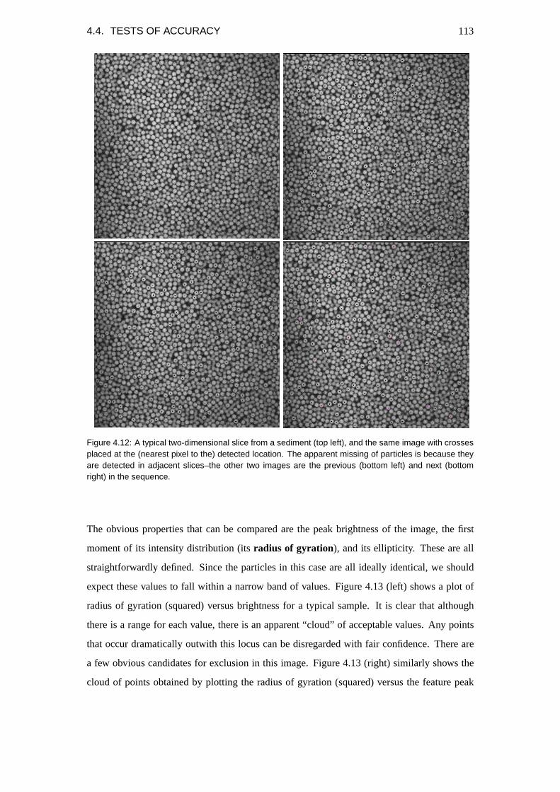
4.4. TESTS OF ACCURACY 113
Figure 4.12: A typical two-dimensional slice from a sediment (top left), and the same image with crossesplaced at the (nearest pixel to the) detected location. The apparent missing of particles is because theyare detected in adjacent slices–the other two images are the previous (bottom left) and next (bottomright) in the sequence.
The obvious properties that can be compared are the peak brightness of the image, the first
moment of its intensity distribution (itsradius of gyration), and its ellipticity. These are all
straightforwardly defined. Since the particles in this case are all ideally identical, we should
expect these values to fall within a narrow band of values. Figure 4.13 (left) shows a plot of
radius of gyration (squared) versus brightness for a typical sample. It is clear that although
there is a range for each value, there is an apparent “cloud” of acceptable values. Any points
that occur dramatically outwith this locus can be disregarded with fair confidence. There are
a few obvious candidates for exclusion in this image. Figure 4.13 (right) similarly shows the
cloud of points obtained by plotting the radius of gyration (squared) versus the feature peak

114CHAPTER 4. PARTICLE COORDINATES FROM THE CONFOCAL MICROSCOPE
intensity value. This technique is reasonable, but in fact it is also unreliable. It is not clear
Figure 4.13: Two example “clouds” found by plotting the radius of gyration squared of a feature versus itstotal brightness (left), and the radius of gyration squared of a feature versus its peak brightness. Sincethe particles are supposedly identical, these properties should fall within a tight locus. Several pointsclearly belong to rogue particles (which may nonetheless be genuinely very much different from thetypical particle).
what the acceptable locus is, and it is never obvious from the data, even for very good quality
images, where the cutoff should occur. Furthermore, it is never able to indicate which particle
coordinates are reliable on an individual basis. Once again, this check can be useful in certain
cases, and in particular it has the significant advantage that it takes into account properties of
individual particles, but it is still clear that we require an objective measure whose value and
acceptable variation is knowna priori.
Pixel Biasing
In the spirit of the above measure, which focuses on the acceptable properties of the particles
considered as a whole, there is another measure that can indicate a systematic problem in the
particle location.
Since all of the techniques we consider here start by finding the nearest pixel to the genuine
particle centre and then refining this first estimate, there can be a tendency towards (or in some
cases even away from) integer coordinates. The way in which this occurs can differ depending
on the algorithm, but in a typical sample, the fractional part of the particle coordinates ought to
be distributed evenly from zero to one. By plotting the histograms of the fractional part of the
x-, y-, and z-coordinates separately, one can check that these are indeed flat. If they are not,
then there is clearly some problem in the technique, which must be explained. This measure
gives no indication of the problem, but may still be useful in identifying a systematic error in
the technique. Figure 4.14 shows three particularly nice histograms of the fractional parts of

4.5. CENTROIDING 115
Figure 4.14: The fractional part of the coordinates for a set of features found using the centroiding tech-nique. These are particularly flat distributions and suggest that the window size used was appropriate.
the feature coordinates for the centroid technique.
Other possibilities
There are undoubtedly other similar statistical properties which could be used to assess how
good the coordinates appear to be. One other is the local volume fraction, which, in the case
of a homogeneous sample, ought to be the same (within a certain distribution) for all of the
particles. We discuss this in more detail in Section 5.2.4, but once again, it is not particularly
useful as we do not know what degree of variation is acceptablea priori. Once more, we really
desire a quantitative measure of how well each particle’s image matches the expectation.
Assessing the Accuracy of each Determined Particle Coordinate
We have reiteratedad nauseamthe benefit that would be provided by having an objective
quantitative measure of goodness-of-fit that could be applied to each particle. Ultimately, av-
erage quantities are something that quantitative confocal microscopy expressly seeks to avoid;
it seems much better to have a local criterion for assessing accuracy.
One of the successes of this thesis is that we now have available a technique based on just such
a tool. We discuss this in the Section after next, but first, to appreciate its benefits, we now
discuss the previous best particle location technique.
4.5 Centroiding
Particle location in dense colloidal systems based on a centroiding technique has been shown
to be useful in a number of publications (for example the previously cited papers of Weeks
and Weitz, see also other papers from these groups [77, 78, 79]). Although the technique

116CHAPTER 4. PARTICLE COORDINATES FROM THE CONFOCAL MICROSCOPE
has been widely used, few details have been published on the mechanics of its application to
colloidal systems. In this section we discuss the technique as it has been used so far, but also
go considerably further in discussing its application to colloidal systems in three dimensions
than has so far appeared in print.
4.5.1 A brief literature review
The centroiding method that has been used here is based on the work Murray and Grier [136,
and their further papers cited therein], and which evolved into the widely-cited reference paper
of Crocker and Grier [118]. The routines used here are as modified by Weeks. This paper gives
a good description of the technique as applied in two dimensions to colloidal samples. They fail
to mention, however, that this paper describes a method which is well documented, and indeed
applied in much more sophisticated forms, in other fields. Most notable of these is particle
image velocimetry (PIV), in which roughly-Gaussian shaped peaks are found (admittedly these
are formed differently; they are instead correlation peaks, but the method of locating them is
identical) [137]. A good general introduction to centroiding (and other techniques) in PIV is
given by Raffelet al. [132]. A very good description of the accuracy of centroiding as applied
to PIV can be found in Bolinder [135]. There are many papers dealing with centroiding in more
detail, covering aspects such as optimum algorithm in the presence of noise ([138, 139]), and
the importance in dealing with noise of the so-called thresholding step [140]. (This is discussed
further below.) More sophisticated PIV algorithms use for example the three-point estimators
discussed in 4.3.1 ([137, 132]), including iterative techniques [141].
The basic centroiding algorithm as used by Crocker, Grier, Weeks, and us is very straight-
forward, and in what follows we need not appreciate the full complexity of these methods.
However sophisticated they become, they all seek to find with maximum accuracy the centroid
of an image distribution. We discover shortly that this is not exactly what we desire.
4.5.2 Basic technique and parameters
Here we discuss the basic algorithm used to find particle coordinates using the centroiding
technique.
The image is first filtered according to§4.2.2. We then follow the discussion of§4.3.1, where
the refinement step is the simple centroid procedure.
4.5. CENTROIDING 117
To find the candidate particle locations, that is, the nearest pixel (integer) to the “true” location,
we search the image for local maxima. Local maxima are simply the brightest points within
a three-dimensional region of sizeseparation×2, whereseparationis a 3- element vector.
Typically, since the particles are of sizer'1µm, and the pixel pitch is'0.15µm pixel −1 in
the x- and y-directions and'0.2µm pixel−1 in the z-direction, the particle image will be in the
region of13 pixels square by10 pixels deep. The parameterseparationis always an integer
vector, and may be odd or even.
Once the candidate particle locations have been determined, a region (orwindow) of sizeextent
is considered around each in turn. For technical reasons (related to the familiar image process-
ing problem of desiring a unique central pixel in an image), the windows are always an odd
integer size in each direction; they are always the next smallest odd integer above that actu-
ally desired, so thatextent'[13.0, 13.0, 11.0]. The centroid of the image intensity distribution
is then taken within this window, giving the final particle coordinate. It is straightforward to
calculate basic properties here of the distribution of intensity (total brightness, peak brightness,
and radius of gyration) within this window.
There is an additional parameter,threshold, which turns out to be important, and was always
used. In a crude attempt to address the problem that occurs when two particles come close
to one another,thresholdallows the user to ignore all pixels within the window specified by
extentthat fall below a fraction (≡threshold) of the peak height belonging to that particle. All
of the statistics returned on the particle refer only to pixels having intensity greater than peak
intensity× threshold. If thresholdis specified, then the code also returns, for each particle, the
proportion of pixels within regionextentwhich lay above the threshold.
Lastly, the feature location code as supplied to us has hard-wired into it the condition that any
local maximum, that is, candidate particle location, whose maximum intensity is less than70%
of the brightest peak in the image is disregarded. This is an arbitrary figure, but was kept here.
The centroid technique used was therefore extremely simple. We have found, however, that
it is nonetheless quite powerful, and in particular very robust to variations in the choice of
parameter. We discuss the choicece of input parameter next.
4.5.3 Parameter Optimisation
In this section we discuss the effect of changing the various parameters on the quality of the
datasets returned. We use one particular fairly high quality dataset, which is the sediment

118CHAPTER 4. PARTICLE COORDINATES FROM THE CONFOCAL MICROSCOPE
of a batch of ASM246 particles imaged using the BioRad confocal microscope. This is a
512× 512× 100 image at a pixel pitch of[0.16, 0.16, 0.2].
The parameter space is enormous, so only a selection of parameter choices are shown here. We
emphasise that this is for one particular high quality image, and the relative importance of cer-
tain parameters (particularlythreshold) varies with the exact system under study. Nonetheless,
the discussion here applies to all of the systems and imaging parameters I have used.
Figure 4.15 shows the colour table used in illustrating the parameter optimisation procedure.
0 255
Figure 4.15: The colour code used to illustrate changes in the rdf for various centroid technique parame-ters.
Extent Parameter
Figure 4.16 shows the effect of changing the parameterextent, which instructs the centroid-
ing procedure what size of region it should consider about each candidate particle location
in attempting to refine that coordinate. This Figure shows that the exact choice ofextentis,
Figure 4.16: The effect of varying the “extent” parameter as defined in the text. This parameter is in somesense the most important in the centroiding technique.
surprisingly, not critical. The size of the window must be chosen by eye from the original
images, and this result is encouraging in revealing that a two-pixel error either way (which
is in fact a huge error in absolute distance terms) is not critically important. The supposedly
“best” value determined by eye was[13.0, 13.0, 11.0]. This is shown in black in Figure 4.16.
The next largestextentshown is[15.0, 15.0, 13.0], which is very similar, with the larger be-
ing slightly better. The caseextent=[11.0, 11.0, 9.0] is shown in cyan. This is not as good,
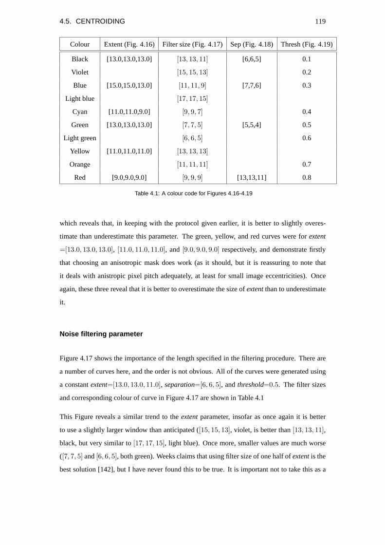
4.5. CENTROIDING 119
Colour Extent (Fig. 4.16) Filter size (Fig. 4.17) Sep (Fig. 4.18) Thresh (Fig. 4.19)
Black [13.0,13.0,13.0] [13, 13, 11] [6,6,5] 0.1
Violet [15, 15, 13] 0.2
Blue [15.0,15.0,13.0] [11, 11, 9] [7,7,6] 0.3
Light blue [17, 17, 15]
Cyan [11.0,11.0,9.0] [9, 9, 7] 0.4
Green [13.0,13.0,13.0] [7, 7, 5] [5,5,4] 0.5
Light green [6, 6, 5] 0.6
Yellow [11.0,11.0,11.0] [13, 13, 13]
Orange [11, 11, 11] 0.7
Red [9.0,9.0,9.0] [9, 9, 9] [13,13,11] 0.8
Table 4.1: A colour code for Figures 4.16-4.19
which reveals that, in keeping with the protocol given earlier, it is better to slightly overes-
timate than underestimate this parameter. The green, yellow, and red curves were forextent
=[13.0, 13.0, 13.0], [11.0, 11.0, 11.0], and [9.0, 9.0, 9.0] respectively, and demonstrate firstly
that choosing an anisotropic mask does work (as it should, but it is reassuring to note that
it deals with anistropic pixel pitch adequately, at least for small image eccentricities). Once
again, these three reveal that it is better to overestimate the size ofextentthan to underestimate
it.
Noise filtering parameter
Figure 4.17 shows the importance of the length specified in the filtering procedure. There are
a number of curves here, and the order is not obvious. All of the curves were generated using
a constantextent=[13.0, 13.0, 11.0], separation=[6, 6, 5], andthreshold=0.5. The filter sizes
and corresponding colour of curve in Figure 4.17 are shown in Table 4.1
This Figure reveals a similar trend to theextentparameter, insofar as once again it is better
to use a slightly larger window than anticipated ([15, 15, 13], violet, is better than[13, 13, 11],
black, but very similar to[17, 17, 15], light blue). Once more, smaller values are much worse
([7, 7, 5] and[6, 6, 5], both green). Weeks claims that using filter size of one half ofextentis the
best solution [142], but I have never found this to be true. It is important not to take this as a
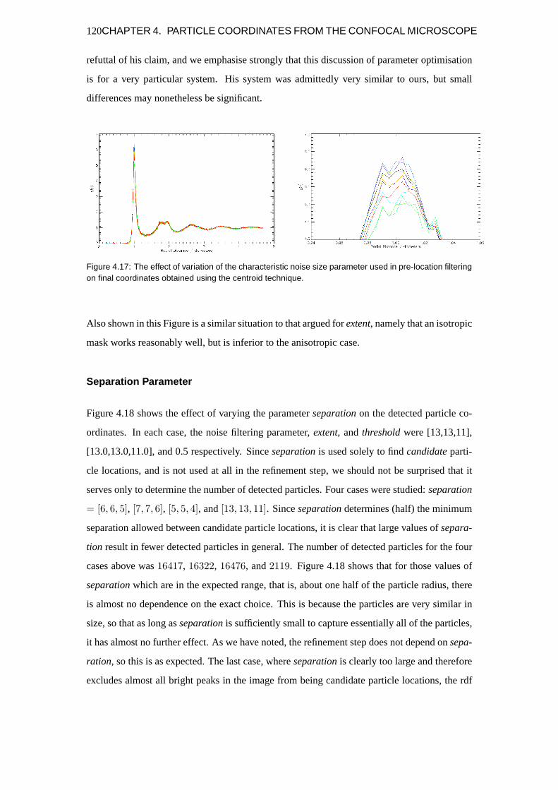
120CHAPTER 4. PARTICLE COORDINATES FROM THE CONFOCAL MICROSCOPE
refuttal of his claim, and we emphasise strongly that this discussion of parameter optimisation
is for a very particular system. His system was admittedly very similar to ours, but small
differences may nonetheless be significant.
Figure 4.17: The effect of variation of the characteristic noise size parameter used in pre-location filteringon final coordinates obtained using the centroid technique.
Also shown in this Figure is a similar situation to that argued forextent, namely that an isotropic
mask works reasonably well, but is inferior to the anisotropic case.
Separation Parameter
Figure 4.18 shows the effect of varying the parameterseparationon the detected particle co-
ordinates. In each case, the noise filtering parameter,extent, andthresholdwere [13,13,11],
[13.0,13.0,11.0], and 0.5 respectively. Sinceseparationis used solely to findcandidateparti-
cle locations, and is not used at all in the refinement step, we should not be surprised that it
serves only to determine the number of detected particles. Four cases were studied:separation
= [6, 6, 5], [7, 7, 6], [5, 5, 4], and[13, 13, 11]. Sinceseparationdetermines (half) the minimum
separation allowed between candidate particle locations, it is clear that large values ofsepara-
tion result in fewer detected particles in general. The number of detected particles for the four
cases above was16417, 16322, 16476, and2119. Figure 4.18 shows that for those values of
separationwhich are in the expected range, that is, about one half of the particle radius, there
is almost no dependence on the exact choice. This is because the particles are very similar in
size, so that as long asseparationis sufficiently small to capture essentially all of the particles,
it has almost no further effect. As we have noted, the refinement step does not depend onsepa-
ration, so this is as expected. The last case, whereseparationis clearly too large and therefore
excludes almost all bright peaks in the image from being candidate particle locations, the rdf

4.5. CENTROIDING 121
Figure 4.18: The effect of varying the “separation” parameter as discussed in the text. This parameter iscrucial in determining how many particles are found in the sample.
is correspondingly both noisier (as it is based on many fewer particles), but also has its peak
shifted to large values (reflecting that the analysis is claiming to find a subpopulation of larger
particles). The peak has moved to around5% larger than for the “optimum” parameters, and
about10% of the particles identified previously are still found. These figures are reasonably
convincingly close to the expectation of around a polydispersity of around6%.
Threshold Parameter
Figure 4.19 shows the effect of varying the threshold parameter. Although this parameter has
been found to be crucial in some samples, its effect is relatively limited here (Figure 4.19 (left)).
Closer inspection of the first peak reveal that it does have a small effect. The colour code is
Figure 4.19: The effect of variation of the “threshold” parameter as defined in the text.
as used before (Figure 4.15), and the results are shown for threshold values of0.1, 0.2, 0.3,
0.4, 0.5, 0.6, 0.7, and0.8. Here the noise filtering parameter,extent, andseparationwere kept

122CHAPTER 4. PARTICLE COORDINATES FROM THE CONFOCAL MICROSCOPE
constant ([13, 13, 11],[13.0, 13.0, 11.0], and[6, 6, 5] respectively).
The bluest curves (low threshold) have relatively low peak height. Higher values of threshold
give greater peaks (the two green peaks have threshold value0.5 and0.6). The highest thresh-
old values have lower first peak heights (reddest curves). This is relatively easy to understand.
The purpose of the threshold parameter is to disregard pixels which are unlikely to belong to
the bright peak of the particle under consideration. This is very crude and we discuss a better
solution later. However, it is successful to an extent, as evidenced by the increase in the first
peak height with increasing threshold parameter. When the threshold parameter becomes large,
however, the centroid estimate is based on very few pixels and therefore becomes less reliable.
A compromise value of somewhere in between is therefore advisable. A previous similar study
to this one, but on a crystalline sample, found the threshold parameter more important; under-
standably this is sample dependent, but a value of' 0.5 is generally a good choice. In this
thesis,0.5 was always used.
Although I believe that the trends shown above are generally appropriate for studies of colloidal
systems, and certainly reflect the experience I have had with all of the samples I have tried, it
is important to reiterate that a similar analysis should be performed for all new systems. As
well as ascertaining that the general behaviour is similar for other systems, it is important to
establish the sensitivity in each case.
4.5.4 An Appraisal of the Centroiding Technique
The centroiding technique that has now been widely used is clearly successful, at least in
some circumstances. In particular, the radial distribution functions found from density-matched
crystalline samples are convincing. However, there are two problems with this technique.
The first is simply that there is no way of assessing its accuracy. A radial distribution function
showing a sharp first peak, with few particles at radial separations of less than one diameter is a
reasonable indication of accuracy, but this is not really satisfactory. In the majority of samples
studied in this enquiry, the peaks are rather broad and begin to rise lower than one would expect
(typically around70% of one diameter). When this is the case, it is impossible to determine
whether this is a feature of the sample, or a result of the analysis performing less well than
expected. Since the samples are believed to be of nearly-hard spheres, it is often suspected
that the fault lies with the centroiding technique. Weeks and others claim an accuracy for the
technique of around30nm in the lateral directions and50nm in the axial one (for example,

4.6. WHY THE CENTROID IS NOT THE PARTICLE CENTRE 123
[77]), but these figures have never been justified in print. Presumably these are some sort of
best case, since the success of the technique is highly sample dependent (particularly with
respect to the degree of index-matching in the sample) and to the noise in the image, and the
dynamic range occupied by the particle image. What is required is a convincing means of
assessing how accurately each particle has been located.
The clue to the second problem follows from the above. Theprecisionwith which particle
centres have been found can be inferred by plotting the radial distribution function with in-
creasingly small bins of radial distance. Smaller bins mean fewer particles in each, and hence
noisier data, but also narrower peaks in the distribution. Assuming the sample contains suffi-
ciently many points, then reducing the bin size will result in a successively sharper distribution
until the bin size corresponds to the mean precision to which the particle coordinates are known,
whereupon further bin size reduction will result in a noisier curve but with the same underlying
shape. This gives a reasonable measure of the precision to which the centroid positions are
known. This precision is typically around30–40nm for the samples used in this enquiry, which
at first seems reasonable when compared with the published claims for accuracy. However,
the important assertion of this section is that the precision to which the positions of the cen-
troids of particle brightness are known is not the same as the accuracy with which the particle
coordinates are known. This is because
the centroid of a particle image’s brightness isnot necessarily the centreof
that particle.
This is a fairly obvious consequence of imaging objects that are close in size to the resolution
of the microscope, and we discuss this in more detail in the next section. It is interesting to note
that not everyone appreciates this important distinction; witness the assertion that the accuracy
of the centroiding procucedure can be inferred fromg(r) ([143],p.S4151). We now explain
why this is not the case.
4.6 Why the Centroid is not the Particle Centre
Section 3.6 gave an indication of what the image of a sphere, the SSF, should be for a micron-
sized sphere. The important point is that the “smearing” of the sphere due to the diffraction
limit results in a SSF that is larger in extent than the sphere actually is. In the case where the

124CHAPTER 4. PARTICLE COORDINATES FROM THE CONFOCAL MICROSCOPE
spheres are well separated, this is of no consequence. However, when the spheres are close to
one another, the SSFs overlap. This section illustrates that this effectdoesaffect detrimentally
the centroiding technique, and motivates a solution.
4.6.1 Illustration of the problem
Figure 4.20 shows the intensity profile through a typical modelled SSF in a lateral plane (left-
hand image) and an axial one (right-hand image). This modelled SSF was generated as de-
scribed in Section 3.6, using a Gaussian PSF of x-y extent300nm and z extent600nm, and
assume a sphere diameter of2µm. The centroid of the brightness (within a window of size
11-13, typically) corresponds to the centre of the particle (within uncertainty due to noise and
digitisation errors).
Figure 4.20: The simulated intensity profile of a 2µm diameter particle in the lateral plane (left) and axialdirection (right). The axes in this and the remaining figures in this section are in pixels, with a pixel pitchof 0.2µm per pixel. Note the substantial broadening of the image of the sphere relative to the true size ofthe particle (which is 10 pixels).
Figure 4.21 shows the case where two particles are too close to one another. “Too close”
depends on the resolution along the particle direction of the line of centres of the particles. In
this case, the intensity distribution in the centroid window is clearly asymmetric, and, as such,
the centroid does not correspond with the true sphere centre. As indicated in Figure 4.21, the
net effect of this is to suggest feature centres that are too close together. This is in keeping
with the first peak of the radial distribution function beginning to rise too early. In fact, the
situation shown in Figure 4.22 is the case where the two particles are touching (the centres are
at 50 and60 pixels, which corresponds to a separation of2µm). Figure 4.22 (left) shows that
in the case where the two particles lie in the lateral plane, in the absence of noise and for two

4.6. WHY THE CENTROID IS NOT THE PARTICLE CENTRE 125
10 pixels
apparentlocationlocation
true
Figure 4.21: A schematic illustration of the effect of overlapping SSFs on the centroid position. The right-hand image shows the important region, where it is clear that overlapping SSF tends to find the particlecentres too close together.
identical particles, the intensity along the line of centres of the particles falls to about57% of
peak intensity, which is probably acceptable.
Figure 4.22: Simulated intensity profile through two particles in contact, both in a lateral plane (left) andan axial one (right).
Figure 4.22 (right), on the other hand, illustrates the same situation for two particles that are
touching and in the axial plane i.e. two vertically-stacked particles. In this case, the intensity
along the line of centres falls only to around90% of peak intensity. This is clearly far too little
to be able to apply the centroid window acceptably. Bearing in mind that the noise level in
these units is typically around30-40 greylevels, there is essentially no distinguishable drop in
the intensity between these two particles.
Figure 4.23 shows the situation in a “reasonably” dense sample, where the particle images
overlap, but to such an extent that the technique is probably not compromised; in these cases
the centroid of intensity within the centroid window does correspond to the particle centre.
It should also be recognised that these figures represent the best case, where both features have
the same peak height and noise has no effect.

126CHAPTER 4. PARTICLE COORDINATES FROM THE CONFOCAL MICROSCOPE
Figure 4.23: Simulated intensity profile in the vertical direction for two particles which are close but nottouching. This is probably at the border of acceptability, and corresponds to a vertical separation ofaround 1.3 diameters.
This section has therefore illustrated why the centroiding technique cannot be relied upon in
dense suspensions. Exactly where the problem comes is not cleara priori, but probably lies
somewhere between Figures 4.22 (right) and 4.23. Certainly, it becomes increasingly important
as density increases. The effect will become important first for particles which come close in
the vertical direction. Figure 4.23 probably gives a reasonable estimate of the point at which
the error begins to manifest itself. We can obtain a very rough estimate of the volume fraction
at which this will occur by using a simple argument. Suppose we take a close-packed crystal
(Φcp = 0.74) and steadily reduce the volume fraction by giving each particle more space. If
we view the particle, radiusr, as occupying a cubic box of sidea, then the volume fraction
is Φ ∝ (ra
)3. To get a very crude idea of when the above effect becomes important, we
substitute the separation of the two particles indicated in Figure 4.23, which is3 pixels (that is,
a = 1.30acp), for the mean interparticle spacing to the above relationship, to get an estimate
of the important volume fraction:
Φ =(acp
a
)3Φcp = 0.34.
So this effect will begin to manifest itself far earlier than one might expect. Of course, often
there is no ordering and so there will be occasionally particles too close together even at much
lower volume fractions. Furthermore, this estimate of the onset of the problem does not take
account of the fact that where it first occurs, its effect is liable to be very small. There is no
way we have thought of which can establish where it first becomes important.
In some respects, the best and most obvious way to avoid this problem is the approach of van
Blaaderen (e.g. [76]), namely to use so-called “core-shell” particles. These are cleverly syn-
thesised spheres with a fluorescent core and (otherwise identical) non-fluorescent shell. The

4.6. WHY THE CENTROID IS NOT THE PARTICLE CENTRE 127
non-fluorescent shell is large enough that even in the case when one particle lies directly on
top of the other, the SSFs do not overlap significantly. The disadvantage of this approach is
that core-shell particles are more difficult to obtain, and were not available in this investiga-
tion. Furthermore, core-shell particles necessarily have fewer bright pixels per particle, so it
may be necessary to oversample the images to provide sufficient data to allow the centroid-
ing procedure to work. A more significant problem is that of polydispersity; the cores can be
polydisperse independently of the particles. Perhaps worse is the potential situation where the
cores are monodisperse but the whole particles are not. This would lead to the impression of a
monodisperse system, and care must be taken not to be fooled by this. In general, however, the
advantage of core-shell particles almost certainly overcomes these potential difficulties.
Nonetheless, even with solidly-fluorescent particles, it is possible to achieve particle coordi-
nates reliably by employing a more sophisticated fitting procedure, as described earlier (§4.3.1
and onwards).
An important related story
We have argued strongly that other authors have disregarded an important feature of confocal
microscopy of colloids, which arises from the fact that the image of a particle is larger than the
particle itself. Here we have argued that this in general leads to particle centres being deemed
too close together.
This problem is not specific to confocal microscopes, and in fact since we began investigating
this effect, another group have suggested that it has been responsible for a significant con-
troversy in soft matter physics. Some groups have argued in favour of so-called like-charge
attraction (LCA), that is, an apparent attraction between colloidal particles of like charge under
certain (quite specific) experimental conditions (see, e.g. [143]). The group of Bechinger have
demonstrated that the overlap of particle SSFs (my terminology) can result not only in an ap-
parent separation less than the true separation (the effect I have described), but also one larger
than the true separation [120]. This case arises because the intensity profile of a single particle
has negative (that is, less than the background) portions for a normal brightfield microscope,
§3.5, rather than the always-positive Gaussian form I have used for the simple model used
here. Nonetheless, this paper vindicates what I have argued. It is worth emphasising that my
work is genuinely three-dimensional, as opposed to these (pseudo-)two-dimensional studies,
and applies to confocal microscopy. They specifically question whether this effect applies to

128CHAPTER 4. PARTICLE COORDINATES FROM THE CONFOCAL MICROSCOPE
the confocal case; I would argue that the discussion above shows that it certainly does, and in
particular justifies the claim that it is typically even more important, since confocal studies are
more likely to attempt three-dimensional studies.
* * *
Both of the problems described in this section, firstly that there is no means of assessing the
accuracy of the position of each particle, and secondly that the centroid does not accurately
coincide with the true centre of the particle can be neatly dealt with using one particular scheme
of refinement. We will refer to this as SSF refinement, and in the next section demonstrate that it
can be used to provide particle coordinates with a great deal more confidence than the centroid
procedure.
4.7 SSF refinement: Using the SSF to refine particle coor-
dinates
The centroiding procedure undoubtedly produces tolerable results even for the most dense
packings of non-core-shell particles. This much is clear from the large number of publications
on colloidal glasses, but also from experimental data in this enquiry. Figure 4.24 (left) shows a
rdf from a glassy sediment, from which it is obvious that the centroiding procedure has worked
acceptably. Figure 4.24 (right) shows a similar sample, but for an image of lower quality (i.e.
noisier) of the sort that you would get at a higher capture speed. In this case, the rdf is less
convincing, but still obviously “nearly right”. This Figure reveals that these samples do give
rise to good rdfs under the right imaging conditions, and that any poor quality rdfs which we
obtain are due to the particle location rather than the sample itself.
To proceed, then, in improving these coordinates, it is necessary to assess how likely each
calculated particle location is to be an accurate reflection of the particle’s true location. This
is best achieved by comparing the locality of supposed particle locations with the “expected”
SSF. The standard way of doing this is using the chi-square test to compare the vicinity of
the particle in the original image with the expected SSF. We do not use the calculated SSF
from earlier, which was always intended to be a schematic illustration rather than a realistic
simulation. Instead we use a SSF extracted from the actual data.

4.7. SSF REFINEMENT: USING THE SSF TO REFINE PARTICLE COORDINATES129
Figure 4.24: A comparison of the radial distribution functions found for a good quality (left) and a mediocrequality (right) image of two similar glassy samples, as determined using the centroid procedure.
4.7.1 Achieving a satisfactory SSF
The best way to achieve a realistic approximation to the image of a particle is to image a large
number of lone particles and form an average image of these. By definition, it is difficult to
achieve a lone, sufficiently slow-moving colloidal particle. Moreover, this approach would
require having a reference sample measured separately from the image capture, and would not
reflect the image of the particle in the true sample at the time of image capture.
A convenient compromise is to extract an approximation to the ideal SSF from each dataset.
This has the advantage that the SSF is definitely representative of the images of particles in
each dataset. In addition, in principle any aberrations in the imaging system can be measured
directly. For example, the index mismatch between the sample and the immersion oil causes
a spherical aberration that becomes worse with increasing depth. In this instance, the SSF
becomes a function of depth; this can in principle be dealt with using this approach. This was
not done here.
To extract the SSF, a region of appropriate size is considered about each of the (nearest integer)
positions as determined by the centroiding technique. At this stage, it is assumed that these are
all reliable, to nearest pixel. The mean intensity of these is then taken as the SSF. It is worth
noting that the the resultant SSF is virtually unchanged regardless of whether the average is a
number- or intensity-weighted one.
Most importantly, the SSF determined in this way is necessarily broader than the “true” SSF,
due to the crude averaging. However, the results achieved using this approximation are good.

130CHAPTER 4. PARTICLE COORDINATES FROM THE CONFOCAL MICROSCOPE
4.7.2 Assessing the accuracy of each particle location
Having established what the vicinity of each particle ought to look like, it is algorithmically
straightforward to step through each of the (nearest integer) positions determined by the cen-
troiding technique, and calculate the sum of (squared) differences between the measured image
and the expected SSF. This gives a raw number to each particle, which is a first estimate of how
well that particle location approximates the particle’s true position. However, it is not par-
ticularly useful in discriminating between “good” and “bad” particles, since it deals with the
nearest pixel rather than the actual determined position.
If the detected image is
Iim(x′, y′, z′),
with (x′, y′, z′) being the indices to the pixels in the image (i.e.0≤x′, y′≤511, 0≤z′≤99 for a
512 x 512 x 100 image), and
ISSF (x′′, y′′, z′′)
is the “ideal” sphere spread function, with its own image coordinates0≤x′′≤extent(0), 0≤y′′≤extent(1),
0≤z′′≤extent(2), where extent is the size of the SSF, then the sum of squared differences for
particlei is:
s2(i) =∑
x′′,y′′,z′′
[ISSF (x′′, y′′, z′′)− Ifeature(i)
]2, (4.6)
with the sum running over allx′′, y′′, andz′′.
HereIfeature(i) is the region of the original image surrounding the detected (nearest pixel)
position of particlei, fint(i) = (x′i, y′i, z
′i):
Ifeature(i) = Iim
(x′i−
wx
2: x′i+
wx
2, y′i−
wy
2: y′i+
wy
2, z′i−
wz
2: z′i+
wz
2
),
with w = (wx, wy, wz) the windoww =[extent−(extent mod2)], allowing for the grid coor-
dinates which include a grid point(x′′, y′′, z′′) = 0.
In fact, to perform the comparison between the image of a sphere and the measured SSF, care
has been taken to ensure that they are both normalised in the same way. Whilst it is desirable
for all features to occupy the same proportion of the instrument dynamic range, this is not
usually possible for dense samples. In particular, particles deeper in a stack are considerably
less bright than shallower ones. To perform the comparison, the extracted feature brightness
is scaled by ratio of its peak height to that of SSF. The SSF is normalised to occupy the entire

4.7. SSF REFINEMENT: USING THE SSF TO REFINE PARTICLE COORDINATES131
range of greyscales. Note that the presence of noise in the measured image means that this is
an approximation; a more sophisticated normalisation would operate on more than one point,
but even without this the procedure works well.
Chi-square
The sum of square differences is, it turns out, sufficient to implement significant improvement
in particle location. However, the more usual measure is the so-calledchi-squarevalue. This
is defined via:
χ2(i) =∑
x′′,y′′,z′′
[ISSF (x′′, y′′, z′′)− Ifeature(i)]2
σ2x′′,y′′,z′′
. (4.7)
The difference between chi-square and the simple sum of square differences is the value
σx′′,y′′,z′′ , which is the uncertainty associated with each point. In this thesis,σx′′,y′′,z′′ = σ
is constant, so thatχ2 is simply a multiple ofs2, and the two are exactly equivalent for the
purposes in this thesis. The main advantage of chi-square over the sum of square differences is
that it allows a fit to be biased away from those data points which are less trusted, but without
having to disregard them. In this case, brighter pixels have a lower SNR, so could be allocated
a lowerσ value (that is,σ = σ(Iim(x′, y′, z′))). This was not found to be necessary here, but
may represent a future improvement. For the purposes of discussion, the measure used will be
referred to as chi-square, even though it is effectively the sum of square differences.
Whilst this single number is not especially useful, by evaluating it for neighbouring pixels
as well as the supposedly correct one, we achieve achi-square hypersurface. This is a (in
this case) three dimensional array of chi-square values, and will display a minimum near to
the genuine particle centre. Locating this minimum gives a better approximation to the true
location of the particle than the centroiding technique.
4.7.3 Establishing the chi-square hypersurface
To establish the chi-square hypersurface for each particle, the simplest method is to extract
regions of the original imageIim(i) to use in relation 4.7 which are centred on the supposedly
correct pixel, and its nearest neighbours. The number of neighbours to sample is for the user to
choose, but it seems reasonable to assume that the centroiding procedure is accurate to within
2 pixels in each direction: in the worst cases, the first peak of the radial distribution function

132CHAPTER 4. PARTICLE COORDINATES FROM THE CONFOCAL MICROSCOPE
begins to rise at about70% of a diameter, meaning that two contacting particles are judged to
be roughly0.3d too close. This suggests that these are each judged to be around0.15d from
their “true” centres, and bearing in mind that there are typically11-13 pixels representing each
particle, the maximum distance one would expect to find a particle’s supposed centre from its
true one would be approximately0.15 x 13 = 1.95 pixels. In the case of particularly noisy
images, it may be useful to increase this value, but, at least with simplistic algorithms, the
computational complexity increases as the size of the iteration grid cubed.
If the iteration grid has size(δ1, δ2, δ3), then the resulting chi-square is a four-dimensional
array:
χ2(i, j, k, l) =∑
x′′,y′′,z′′
[ISSF (x′′, y′′, z′′)− Ifeature(i, j, k, l)]2
σ2x′′,y′′,z′′
,
where nowfint(i) = (x′i + j, y′i + k, z′i + l) and so
Ifeature(i) = Iim
(x′i+j−wx
2: x′i+j+
wx
2, y′i+k−wy
2: y′i+k+
wy
2, z′i+l−wz
2: z′i+l+
wz
2
),
andj, k, andl take the values{−δ1, ..., δ1}, {−δ2, ..., δ2}, {−δ3, ..., δ3} respectively.
It follows from the above that it is not possible to do this for features which lie within half
of the iteration grid size(δ1, δ2, δ3) of the edge of the dataset, and corresponding care must
be taken in the algorithm. This need not necessarily result in the loss of information, since
the centroiding procedure does not return reliable information from this region anyway; in the
implementation used in this thesis, more information was lost than is absolutely necessary. A
more careful algorithm could be implemented.
Figure 4.25 shows the chi-square values for a randomly-chosen particlei, for slices in x, y,
and z, taken through the hypersurface minimum. In the notation of the above, Figure 4.25
(left) showsχ2(i, ∗, k, l) for thex andy coordinates for whichχ2 is minimised, and where the
asterisk denotes all values ofj. Figure 4.25 (middle) and (right) similarly showχ2(i, j, ∗, l) and
χ2(i, j, k, ∗) respectively. Figure 4.26 shows representations of two-dimensional projections of
the hypersurface onto thex-y plane and thex-z plane.
4.7.4 Finding the chi-square hypersurface minimum
The best location based on the fit to the measured SSF for each particle can be established
in more than one way. The important point here is that we seek to know the coordinates to

4.7. SSF REFINEMENT: USING THE SSF TO REFINE PARTICLE COORDINATES133
Figure 4.25: Slices through the chi-square hypersurface through x (left), y (middle) and z (right) for arandomly-chosen particle.
Figure 4.26: Two-dimensional projections of Chi-square hypersurface for a randomly-chosen particle.Left: x-y projection, Right: x-z projection.
better than nearest pixel accuracy which was the limit of the previous section. There are two
strategies.
Spline fits to the SSF
The first strategy is to produce a fit to the SSF, so that an exact copy can be placed over
the captured image and moved arbitrarily small distances in any direction. This is the most
obvious and apparently best option. It is reasonably easy to implement this to high precision
for analytic functions. However, the SSF is not in general accurately modelled by any simple
analytic function. Spline-fitting functions can interpolate typical SSFs very well (to within1%
of intensity values). Such functions are available in one and two dimensions in IDL, but not yet
in three. These functions allow the user to specify a set ofx values and correspondingy values,
then enter a second set ofx values at which the function should be evaluated. A series of one-
and two-dimensional spline fits were attempted, but the interpolation requirement (spline fits
are extremely unreliable as extrapolations) resulted in a relatively few data points for each, and
as such the results were unacceptably noisy. In any case, it was found that the accuracy of the

134CHAPTER 4. PARTICLE COORDINATES FROM THE CONFOCAL MICROSCOPE
spline fit, though always remarkably good, varied depending on the exact choice of the desired
x coordinates. It was not then possible to be certain if reductions in the measured chi-square
value were due to a better fit, or simply to a change in how well the interpolation scheme had
worked. (In particular, as the calculation of chi-square crossed integer pixel values, since the
necessary data were available without interpolation, the chi-square value dropped as there was
no error in the fit.)
It is likely that at some point three dimensional spline fitting routines will become available for
IDL (competitors already have this); at this point, this approach may be worth reinvestigating.
Interpolation of the minimum
The other strategy for finding the minimum of the hypersurface is simpler, and is the one
which has been shown to be successful here. It simply involves finding the minimum by three
simple interpolations to each of the(2δ1 + 1), (2δ2 + 1) and(2δ3 + 1) data points contained
in slices through the minimum of the hypersurface (typically5 points in each case). This is
less satisfactory in principle than the strategy in the previous section, since it is based on fewer
data points, but turns out to be more robust, and indeed to give convincing results. Moreover,
it would be relatively easy and presumably more reliable to fit through the(2δ1 + 1)× (2δ2 +
1)× (2δ3 + 1) (typically 53 = 125) data points at once. This would represent an intermediate
between these approaches. Nonetheless, even the simplest approach gives good results.
Since there are relatively few data points, it is only reasonable to attempt a simple polynomial
interpolation. This is done using a simple routine POLINT, adapted from the routine of the
same name from Numerical Recipes in C++ [144],§3.1. As with the earlier spline fitting
routine, this routine accepts the known ordinates and corresponding intensity values, as well
as the ordinate value for which the intensity is desired. By repeatedly running this routine
for a large number of points lying within half a pixel of the minimum of the chi-square array,
an array of sub-pixel estimates to chi-square is determined. The lowest-valued entry in this
list corresponds to the best correspondence between the measured SSF and the image of the
feature.
The fineness of the sub-pixel array of points is specified by the user. It is claimed in the
literature that the centroiding technique achieves a best accuracy of around one twentieth to
one tenth of a pixel (of course it does not get anywhere close to this in dense samples; it may
achieve a precision of something approaching this). Once again, the computational complexity
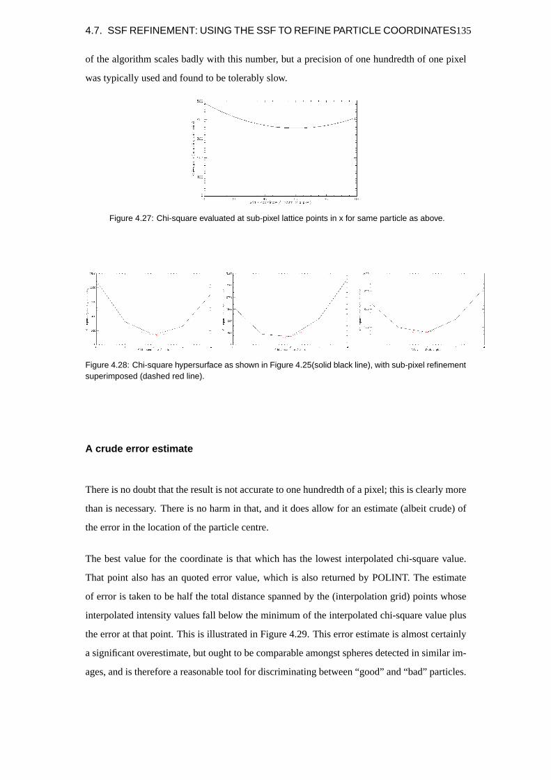
4.7. SSF REFINEMENT: USING THE SSF TO REFINE PARTICLE COORDINATES135
of the algorithm scales badly with this number, but a precision of one hundredth of one pixel
was typically used and found to be tolerably slow.
Figure 4.27: Chi-square evaluated at sub-pixel lattice points in x for same particle as above.
Figure 4.28: Chi-square hypersurface as shown in Figure 4.25(solid black line), with sub-pixel refinementsuperimposed (dashed red line).
A crude error estimate
There is no doubt that the result is not accurate to one hundredth of a pixel; this is clearly more
than is necessary. There is no harm in that, and it does allow for an estimate (albeit crude) of
the error in the location of the particle centre.
The best value for the coordinate is that which has the lowest interpolated chi-square value.
That point also has an quoted error value, which is also returned by POLINT. The estimate
of error is taken to be half the total distance spanned by the (interpolation grid) points whose
interpolated intensity values fall below the minimum of the interpolated chi-square value plus
the error at that point. This is illustrated in Figure 4.29. This error estimate is almost certainly
a significant overestimate, but ought to be comparable amongst spheres detected in similar im-
ages, and is therefore a reasonable tool for discriminating between “good” and “bad” particles.
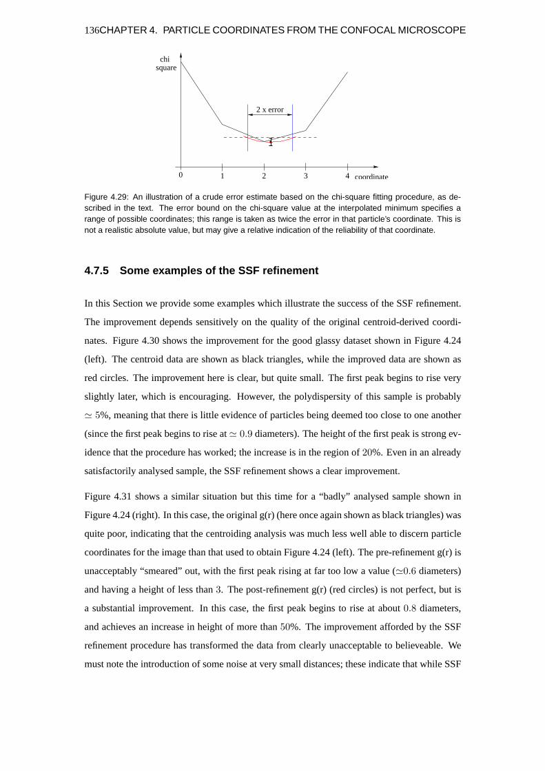
136CHAPTER 4. PARTICLE COORDINATES FROM THE CONFOCAL MICROSCOPE
����
������
��
32
squarechi
1 40 coordinate
2 x error
Figure 4.29: An illustration of a crude error estimate based on the chi-square fitting procedure, as de-scribed in the text. The error bound on the chi-square value at the interpolated minimum specifies arange of possible coordinates; this range is taken as twice the error in that particle’s coordinate. This isnot a realistic absolute value, but may give a relative indication of the reliability of that coordinate.
4.7.5 Some examples of the SSF refinement
In this Section we provide some examples which illustrate the success of the SSF refinement.
The improvement depends sensitively on the quality of the original centroid-derived coordi-
nates. Figure 4.30 shows the improvement for the good glassy dataset shown in Figure 4.24
(left). The centroid data are shown as black triangles, while the improved data are shown as
red circles. The improvement here is clear, but quite small. The first peak begins to rise very
slightly later, which is encouraging. However, the polydispersity of this sample is probably
' 5%, meaning that there is little evidence of particles being deemed too close to one another
(since the first peak begins to rise at' 0.9 diameters). The height of the first peak is strong ev-
idence that the procedure has worked; the increase is in the region of20%. Even in an already
satisfactorily analysed sample, the SSF refinement shows a clear improvement.
Figure 4.31 shows a similar situation but this time for a “badly” analysed sample shown in
Figure 4.24 (right). In this case, the original g(r) (here once again shown as black triangles) was
quite poor, indicating that the centroiding analysis was much less well able to discern particle
coordinates for the image than that used to obtain Figure 4.24 (left). The pre-refinement g(r) is
unacceptably “smeared” out, with the first peak rising at far too low a value ('0.6 diameters)
and having a height of less than3. The post-refinement g(r) (red circles) is not perfect, but is
a substantial improvement. In this case, the first peak begins to rise at about0.8 diameters,
and achieves an increase in height of more than50%. The improvement afforded by the SSF
refinement procedure has transformed the data from clearly unacceptable to believeable. We
must note the introduction of some noise at very small distances; these indicate that while SSF

4.7. SSF REFINEMENT: USING THE SSF TO REFINE PARTICLE COORDINATES137
Figure 4.30: The improvement in g(r) for a high quality image of a glassy sample (Φ'0.64). Note theslight sharpening and increase in height of the first peak.
refinement is clearly an improvement on the whole, it must be introducing a very few “more
wrong” coordinates. This is seemingly disturbing, but very wrong coordinates are easily dealt
with (by ignoring them, usually; it is not difficult to identify pairs of particles whose centres
are separated by less than0.5× diameter). Moreover, since g(r) is formed by dividing byr
(r3 in fact), these points really can originate from very few errant coordinates. We should also
comment here that SSF refinement appears to introduce a greater spread in the data. It is not
obvious to us why this is so, but we note that less precise but more accurate coordinates, which
this evidence suggests, are generally more useful. It is a simple matter to recover the underlying
distributions by averaging over many samples.
The SSF refinement procedure is not specific to any particular dataset. Indeed it should not be;
the technique is very general. Figure 4.32 shows that the improvements are evident over a wide
range of volume fractions, and for differing samples.
Figure 4.32 shows the improvement due to the SSF refinement for systems of the same particles
at three different volume fractions (the three rows), for two different solvent mixtures. We
discuss the systems fully in Chapter 5, but, briefly, here the right-hand column shows samples
where the particles are very nearly refractive index-matched (they are also purposely density-
matched). The left-hand column shows the results for samples which were less well matched.
(For reference, these were PMMA in a mixture ofcis-and cycloheptylbromide and PMMA in
cis-decalin only respectively.)
Consider the two columns separately. At all three densities in the first column (Φ = 0.589,

138CHAPTER 4. PARTICLE COORDINATES FROM THE CONFOCAL MICROSCOPE
Figure 4.31: The improvement in g(r) for a mediocre quality image of a glassy sample (Φ'0.63). Notethe greater sharpening and increase in height of the first peak.
0.4991, and0.4604 from top to bottom), there is a similar dramatic improvement in the coor-
dinates, similar to that shown in Figure 4.31. The comments made there apply here.
The second column data, for samples of density0.5853, 0.5134, and0.4083, also support the
arguments above, since they are very similar to the situation argued in Figure 4.30. The images
of these samples were of higher quality and consequently yielded better centroid coordinates,
so that the refinement process has yielded a less dramatic, though still significant, improvement.
The images with a better refractive index match (right-hand column) are clearly better. As we
discussed earlier, we believe that this is solely due to the particle location rather than different
physical behaviour between the systems. However, we have only justified this remark for
the very highest densities; it is possible here that the effect of charge and or gravity explains
the different shape of g(r). We cannot know for certain, but the important point is that SSF
refinement represents a significant improvement, particularly in the more challenging (greater
refractive index mismatch) samples.
4.7.6 A closer look at fitting
Though SSF refinement appears to work well, it is not quite correct and still suffers from the
same problem as the centroiding technique. Consider Figure 4.33, which shows schematically
how the SSF fitting procedure works. This Figure attempts to illustrate the effect of performing
the SSF refinement for a particle whose SSF overlaps another’s by considering three cases: one
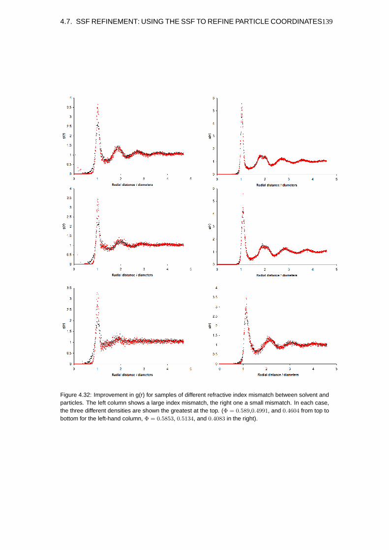
4.7. SSF REFINEMENT: USING THE SSF TO REFINE PARTICLE COORDINATES139
Figure 4.32: Improvement in g(r) for samples of different refractive index mismatch between solvent andparticles. The left column shows a large index mismatch, the right one a small mismatch. In each case,the three different densities are shown the greatest at the top. (Φ = 0.589,0.4991, and 0.4604 from top tobottom for the left-hand column, Φ = 0.5853, 0.5134, and 0.4083 in the right).

140CHAPTER 4. PARTICLE COORDINATES FROM THE CONFOCAL MICROSCOPE
where the overlaid SSF is too far “to the left”, that is, displaced along one coordinate; one
where the SSF is perfectly aligned with the true position of the particle; and one where the SSF
is displaced in the other direction. For a perfectly isolated, noise-free image, this sequence of
events would yield in the first and third cases (assuming the same displacement in each case)
the same non-zeroχ2 value. In the middle case,χ2 would be zero. As the top image in Figure
4.33 shows, in the case where a particle’s image overlaps its neighbour’s,χ2 (indicated by
the shaded area) is never zero. This is not necessarily important; the analysis relies only on
χ2 having a minimum when the true SSF is aligned with the true particle position. However,
this is not necessarily the case. The lower left image shows the effect of a small displacement
����
��
��������
����������������
����������������
���������������������
���������������������
������������������������
������������������������
����������
����������
Figure 4.33: The shaded area in top image shows that there is a non-zero contribution to χ2 even for aperfect match between the true SSF and the (noise free) image when a neighbour is “too close”. This isnot necessarily important, provided that χ2 has a minimum at this point. The lower left image shows adisplacement of the ideal SSF away away from the neighbouring particle; a movement of this sort alwaysincreases χ2. The lower right-hand image, however, while also showing an increasing contribution to χ2,is not so compelling. Depending on the exact shape of these curves, a small movement of this kind canreduce χ2.
along the line of centres of the two adjacent particles, where the displacement isaway from
the neighbouring particle to the one under consideration. In this case, the contribution toχ2,
as denoted by the shaded area, is large. Importantly, not only has the shaded area which was
already present (the right hand one in this Figure) expanded in area, but another shaded area
(to the left) has appeared, and can only grow in size for larger displacements. It is clear from
this that motions of this kind always lead to increasingχ2, as expected.
Motions in the other direction, however, do not necessarily increaseχ2. Consider the lower
right-hand image: in this case, there is again a contribution from the left-hand shaded area
which can only grow for increasing displacement. On the right-hand side of the window, how-

4.7. SSF REFINEMENT: USING THE SSF TO REFINE PARTICLE COORDINATES141
ever, the shaded area here, which is the same shaded area from the top image, has shrunk in
size. This is simply a feature of the shape of the distributions. It is not possible in general to
say whether the reduction in size of the right-hand shaded region is less than the gain in size of
the left-hand shaded region; we must therefore conclude that it could be possible for the mini-
mum inχ2 to occur for some point nearer to the neighbouring particle than the genuine particle
centre. This is the same problem from which the centroiding technique suffered. This is a real
effect, and although we suspect it is less significant than the same effect in the centroiding case
(not least insofar as SSF refinement is an undeniable improvement), it is nonetheless true that
a perfect solution must take account of this effect.
A smart fit: χ2B
We have not developed a modification which can deal with this effect, but we do outline here
some ideas which may prove to be useful.
Consider Figure 4.34, which illustrates how a possible improvement may work. We cannot
avoid the fact that the image of the sphere under consideration is “contaminated” by another
signal (which is added to it). What we aim to do is work out which pixels contain information
originating from the particle only, and not its neighbour. The key improvement over theχ2
method is that we take advantage of oura priori information regarding the shape of the particle
to eliminate certain pixels which cannot be purely from the particle under consideration. As
~250 greylevels ����
������������������
������������������
��noise ~30 greylevels
����������
����������
���
�����������������
����
��
��
����������������������������������������
����������������������������������������
������
������
disregardedregion
this region still contributes
Figure 4.34: A schematic illustration of how χ2B might work. We use a priori knowledge of the shape
of the SSF to eliminate points which cannot possibly originate from the left-hand particle. This meansdisregarding any point which differs from the expected form by more than the known peak noise.

142CHAPTER 4. PARTICLE COORDINATES FROM THE CONFOCAL MICROSCOPE
illustrated in Figure 4.34, since we know the (peak) noise level in the image in general (shown
here to be a typical'10-15% of the feature height), we can say that when the SSF overlay
coincides with the true position of the particle, any pixels whose intensity value lies further
from the expected SSF than the peak noise value cannot belong to that particle, that is, must be
influenced by a neighbouring particle, and is therefore disregarded as unreliable. The remaining
pixels are then used to determine the (weighted) sum of squared differences, which we now
call χ2B (the “B” being for Bayesian, which this method then is). Aχ2
B hypersurface is then
generated from a grid of neighbouring pixels, and whose minimum can be determined in the
same way as above. Figure 4.35 shows that the fit based on this definition ofχ2B has not resulted
in an improvement, although we should note that this procedure has not been been investigated
sufficiently fully to rule out its usefulness.
Figure 4.35: The difference in g(r) between using the SSF refinement procedure described based on χ2,and the argued approach using χ2
B . There is no improvement, and given the doubts expressed aboutthis measure, it is not useful without further development.
This method should make one nervous however, since to some extent it involves rejecting data
we do not like the look of. In particular, it is now possible for a modestly bad fit to have a worse
χ2B than a very bad one, since for very poor fits, there will be few contributions toχ2
B. In the
very worst case, no pixels will be counted, and thereforeχ2B = 0! This is clearly nonsense,
although the idea is seemingly nearly useful. We must therefore find a similar measure, but
one which somehow takes into account the number of pixels used to generateχ2B, as well
as the value ofχ2B. In the simplest form, this could simply beχ2
B per included pixel. A
simpler related possibility is simply to note the number of pixels within the sample window
which lie within the peak noise of the expected value. This is a very simple idea, and involves

4.8. A COMPARISON OF CENTROIDING AND SSF REFINEMENT 143
no argument over what exactly the quantity measured means. When the SSF overlay nearly
corresponds with the true position, there will be a maximum in the number of points counted.
This maximum can be found using the same method as for finding the minimum in theχ2
hypersurface, discussed earlier. Our initial investigations suggest that this method does appear
to work, but is in fact relatively insensitive (the difference in the number of pixels included for
small window displacements is relatively small). The resulting maximum is therefore rather
flat, and its exact position is subject to a large error. Nonetheless, we feel that a combination
of this andχ2B may provide an improvement.
The biggest advantage of knowing the shape of expected particle image is that we can establish
what the image of two overlapping particles should be (for example,§4.6). With an objective
measure of well the data matches the SSF, we could in principle extend the SSF refinement
above to deal with two or more particle centres simultaneously, that is, to fit groups of spheres
in the same calculation. Such an algorithm would identify instances of pairs (or even triplets)
of overlapping particles, then attempt an iterative fit based on adjusting the separation (and
ideally orientation) of two (or more) SSFs simultaneously. This would be algorithmically rea-
sonably tricky, but, more significantly, extremely computationally intensive. It is likely that the
computational time required would be prohibitive.
4.8 A Comparison of Centroiding and SSF Refinement
Section 4.7.5 showed the the SSF refinement is a clear improvement for the samples used in
this enquiry. The argument which we built up to justify trying the improvement only really
considered that this improvement could be due to the problem of overlapping SSFs (Section
4.6), but as Section 4.7.5 showed, it is clear that even the SSF refinement does not adequately
deal with this effect.
We attribute some of the improvement in the particle coordinates (as evidenced by g(r)) to a
small improvement in this problem. We should also point out however that some of the error
in the centroid-derived coordinates is compromised by the presence of noise: despite the noise
filtering step, it is still undoubtedly the case that in some instances, the brightest point of a
particle’s SSF is not the nearest to its true position as a result of single pixel noise. The cen-
troiding procedure uses the brightest point as the nearest-pixel estimate, and then refines this
position, and so is at least one pixel out in some cases. The SSF refinement procedure, by itera-
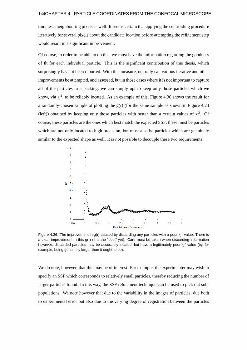
144CHAPTER 4. PARTICLE COORDINATES FROM THE CONFOCAL MICROSCOPE
tion, tests neighbouring pixels as well. It seems certain that applying the centroiding procedure
iteratively for several pixels about the candidate location before attempting the refinement step
would result in a significant improvement.
Of course, in order to be able to do this, we must have the information regarding the goodness
of fit for each individual particle. This is the significant contribution of this thesis, which
surprisingly has not been reported. With this measure, not only can various iterative and other
improvements be attempted, and assessed, but in those cases where it is not important to capture
all of the particles in a packing, we can simply opt to keep only those particles which we
know, viaχ2, to be reliably located. As an example of this, Figure 4.36 shows the result for
a randomly-chosen sample of plotting the g(r) (for the same sample as shown in Figure 4.24
(left)) obtained by keeping only those particles with better than a certain values ofχ2. Of
course, these particles are the ones which best match the expected SSF: these must be particles
which are not only located to high precision, but must also be particles which are genuinely
similar to the expected shape as well. It is not possible to decouple these two requirements.
Figure 4.36: The improvement in g(r) caused by discarding any particles with a poor χ2 value. There isa clear improvement in this g(r) (it is the “best” yet). Care must be taken when discarding informationhowever; discarded particles may be accurately located, but have a legitimately poor χ2 value (by, forexample, being genuinely larger than it ought to be).
We do note, however, that this may be of interest. For example, the experimenter may wish to
specify an SSF which corresponds to relatively small particles, thereby reducing the number of
larger particles found. In this way, the SSF refinement technique can be used to pick out sub-
populations. We note however that due to the variability in the images of particles, due both
to experimental error but also due to the varying degree of registration between the particles

4.9. TRACKING 145
and the sampling grid, this is likely to be realistic only for quite differently sized particles, and
should be used in discriminating between particles belonging to a sample of continuous size
distribution carefully (that is, in typical colloidal samples this is unlikely to be useful).
The SSF refinement procedure I have used is far from perfect. Firstly, the “ideal” SSF is an
average quantity drawn from many particles in each image, and as such is necessarily too broad.
Ideally, a reliable single particle SSF would be ascertained either from a constrained (perhaps
by laser tweezers) particle, or by a much more sophisticated model than I have detailed.
Secondly, the method used to find the minimum of theχ2 hypersurface is not ideal. It is in fact
quite simple, and the interpolation errors are reasonably large. There is surely improvement to
be made here.
Lastly, my implementation of the SSF refinement algorithm is inefficient. This is not really
important, but is an inconvenience which could be improved upon.
These problems are things which we should ideally improve upon, but they do not detract from
the clear success of the analysis. The important thing here is that the measureχ2 has allowed
us to determine when we have managed to improve upon the particle coordinates: this is an
important result of this Chapter.
4.9 Tracking
Having finished discussing how to find particle coordinates in the relevant dense colloidal sus-
pensions, we now discuss briefly some considerations relevant to tracking particles over time.
Really, the success of studying dynamics in these systems relies mostly on being able to identify
particles with confidence in static images, since particles can be tracked simply by capturing
a succession of static images. In principle, this is as simple as taking images twice as quickly
as the dynamical process of interest (once again, to satisfy the Nyquist-Shannon theorem).
There is the additional requirement that dynamical processes must occur on timescales slow in
comparison with the imaging system frame capture rate. There is nothing complicated about
this; it is simply the same requirement that photographers must use when attempting to image
fast processes.
In practice, the imperfect nature of particle tracking means that a particle may not be identified
in one image when it is in a prior or subsequent image. This can occur either because a particle

146CHAPTER 4. PARTICLE COORDINATES FROM THE CONFOCAL MICROSCOPE
is simply missed in one or more frames (most likely due to instrumental noise), or because it
strays from the field of view and then reappears shortly afterwards. It is possible to write an
algorithm which can deal with losing a particle for a few frames and then pick it up again,
identifying it simply by assuming that it has not moved “very far” in the intervening time. This
illustrates a generic problem in particle tracking, that particles cannot be uniquely identified
(they are identical!) There is no way around this, and all tracking procedures work simply by
assuming that no particle moves more than an expected amount between frames. For a very
good tracking algorithm written in the IDL language, and further description, please see Eric
Weeks’ webpage on the subject [145].

Chapter 5
Sample Preparation and
Characterisation
Under the right conditions, colloidal spheres can approximate remarkably well hard sphere
systems. This Chapter discusses two different approximations to hard sphere systems, one
which sediments rapidly and one which does not. In both of these cases, the particles used
were the same. In this Chapter, we discuss these systems in more detail.
The basic requirements are that the particles and solvents have similar refractive indices, both
to minimise the van der Waals attractions between them and to render the samples penetra-
ble by light to sufficient depth to allow (confocal) microscopy. Two solvents were used here,
cis-decalin and cycloheptyl bromide (CHB). Solvents typically cause swelling of the particles;
in this case CHB causes more swelling thancis-decalin. Additionally, it has been shown re-
cently that suspension in CHB causes PMMA particles to acquire a charge. We describe in
this Chapter how the addition of a suitable salt can to some extent counteract this by screening
the charge. As well as describing the particles and solvents used, we discuss how to prepare
samples of known volume fraction reliably, and the uncertainty in the final samples.
For any type of microscopy, the requirement of optimum optical properties place stringent
requirements on the sample cells used. We describe these important properties, and two novel
sample cells which meet them. One of these was developed specifically during the course of
this investigation.
147

148 CHAPTER 5. SAMPLE PREPARATION AND CHARACTERISATION
5.1 System
Particles
The particles used here are made from poly-methylmethacrylate (PMMA, “Perspex”, or “Plexi-
glass”). They are sterically-stabilised by a layer of poly-12-hydroxystearic acid polymer chains
which are chemically attached to the particles. Non-fluorescent particles of this type have been
routinely synthesised for some time at the School of Physics by A.B. Schofield, according to a
recipe described by Antlet al. [146] and Pathmamanoharanet al.. [147].
These particles are not fluorescently-labelled, however. A number of recipes have been pub-
lished for incorporating fluorescent dyes into the particles. The particles used in this enquiry
were synthesised according to the recipe detailed in [148, 149, 150], so that the fluorescent
dye (4-methylaminoethylmethacrylate-7-nitrobenzo-2-oxa-1,3-diazol, or NBD) is chemically
cross-linked into the core of the particle. This is a distinct advantage, since often the fluores-
cence molecules are soluble in the solvent and leach out of the particles over time. Note that the
focus of these papers is really in producing core-shell particles, in which a solidly-fluorescent
such as ours is prepared, and then a non-fluorescent PMMA shell is grown onto the top. While
preferable, core-shell particles were not available in this investigation.
Earlier investigations into particles for use with confocal microscopy tended to focus on other
dyes and materials, for example silica dyed with fluorescein [151, 152] and rhodamine [153].
More recently, Campbell and Bartlett studied several common dyes (DilC18, DiOC18, Nile
Red and Acridine Orange) with PMMA particles. Jardine and Barlett have also produced NBD-
dyed particles similar to those used in this enquiry [154]. These latter two papers between them
conclude that NBD-dyed particles behave well as hard spheres in a mixture ofcis-decalin and
carbon disulphide [154], and that DiIC18-dyed particles also do so in a (near) density-matching
mixture of cycloheptylbromide. The former shows that DilC18 is substantially better in terms
of its photobleaching characteristics than any of the others. However, in this investigation, it
has been found that NBD-dyed particles have very good photobleaching characteristics (i.e.
they do not photobleach significantly over even the longest experiments carried out here.)
Fluorescent Solvent
It is worth mentioning here that there is no reason in principle why the solvent could not be
fluorescent, rather than the particles. In fact, in dense suspensions, in some sense this would

5.1. SYSTEM 149
be preferable, since then a minority of the system would be fluorescent (leading to lower back-
ground). Additionally, in some systems (unlike those studied here), there may be impurities
in the solvent. This may describe a typical industrial system, and in such cases any impurities
in the solvent can frequently be themselves fluorescent. In this case, an overwhelmingly flu-
orescent solvent surrounding non-fluorescent particles would be much more useful. We have
tested as a proof of principle PMMA spheres in EOSIN Y (a typical aqueous dye), and found
convincing images. Figure 5.1 shows a lateral slice through the centre of such a particle (this is
the inverse of the detected image, since the particle location technique requires bright features
on a dark background). Note that water is not a good solvent in which to disperse PMMA, and
only a very low concentration could be achieved.
Figure 5.1: An example of an undyed PMMA sphere dispersed in an aqueous solution of EOSIN Y, awidely-used fluorescent dye.
We should note here also that a similar experiment was carried out on an aqueous Rhodia latex,
which was not fluorescent. Although this sample was substantially more polydisperse than our
samples, it was possible to find particle coordinates by adding dye to the solvent.
The disadvantage of this method is that frequently the dye may be soluble in both the solvent
and the particles, so that it may leach into the particles. This is the same problem that cross-
linking has solved above; the solution in the case of a fluorescent solvent is much more difficult,
since cross-linking the dye molecules “out of the particles” is not realistic.
The particles are designed to be monodisperse hard spheres. In practice, a polydispersity of
around5% is usually achieved. More importantly, these particles are designed to be sterically-
stabilised to behave as nearly hard spheres; whether this is true depends on the solvent used.

150 CHAPTER 5. SAMPLE PREPARATION AND CHARACTERISATION
Solvent
There are three main criteria which characterise whether a given (mixture of) solvent(s) is ap-
propriate. The first and by some way most important of these is that the solvent must maintain
the nearly hard-sphere behaviour of the particles.
Since the particles here are designed to be sterically stabilised, this criterion means that as
well as being a poor solvent for PMMA (so that the particles do not swell significantly), the
suspension medium must also be a good solvent for the PHSA hairs. If this is so, the polymer
hairs are encouraged to adopt extended conformations, which in turn allows them to act as an
almost incompressible barrier.
Once this has been satisfactorily achieved, the solvent must also be chosen to have as near a
refractive index match to the particles as possible. Solvents such as dodecane, while providing a
hard-sphere-like interaction potential, have an unsuitable refractive index (ndodecane=1.42 for
optical experiments, and must be changed. Decalin (a mixture ofcis- andtrans-decalin) has a
suitably close refractive index (n=1.48) for use in many cases. Usually,cis-decalin is preferred
since this has been more widely characterised (and in mixed decalin, the exact composition
varies with different batches.) In light scattering studies, particularly for dense samples, it is
often necessary to do better than this; a mixture of decalin and tetralin is a widely used option
(ntetralin=1.54). It is pretty easy to ascertain when a near-refractive index match is achieved,
since the sample, rather than being “milky”, becomes (slightly ethereally) translucent.
In light scattering studies, the particles are typically much smaller than they are for confocal
studies (r ' 200-500m, as opposed tor & 1µm). Since the gravitational force acting on a
“colloidal” particle is proportional tor3, gravity quickly becomes important at a point some-
where in between the two systems. The density mismatch between the solvent and particles
therefore becomes crucial, and a newdensity-matchingsolvent (or mixture of solvents) must
be found.
For PMMA systems, two mixtures have been used. The first is a mixture of tetralin,cis-
decalin and carbon tetrachloride [155]. The one used in this enquiry is a mixture ofcis-decalin
and cycloheptylbromide (CHB,ρ=1.289g cm−3, n=1.50), which conveniently matches fairly
closely both the density and the refractive index of the solvent with the particles [156].
We should note here that CHB is believed to increase the effective size of the particles over
a period of several weeks [60, 5]. Whether this is due to CHB dissolving the particles very

5.2. SAMPLE PREPARATION 151
slightly, or whether is due to the particles acquiring a slight charge over this time is not clear in
these papers, although Haw has carried out some experiments which appear to settle this issue.
He found that form factors measured on density-matched samples indicate that particles do
swell; he argues that a change in particle charge in the very dilute samples used to measure the
form factor should have no effect, and that the therefore the only explanation for an evolution
in the form factor is a change in the particle size [157].
5.2 Sample Preparation
In this section we detail how to prepare samples from the latices as provided. In general,
this involves changing the solvent, adding salt where necessary to screen any induced charge,
obtaining an estimate of the particle size, and then reliably determining the composition (here
simply the volume fraction) of the stock solution. From here, we must be able to generate
samples of known composition. Each of these stages is considered in turn.
5.2.1 Washing the Colloid
When prepared, the PMMA particles are dispersed in an unsuitable solvent, usually dode-
cane. Dodecane is unsuitable principally because it has an unacceptably low refractive index
(n=1.42). We therefore wish to remove the solvent and replace it with (usually)cis-decalin.
The most straightforward way to replace the solvent takes advantage of the relative density
mismatch between the particles and the solvent. In the case of PMMA (ρPMMA'1.188gcm−3)
suspended incis-decalin (ρcis−decalin'0.897gcm−3), the particles sediment to the bottom of
the container. Once this has happened, a solid “plug” is formed at the bottom, whereupon the
clear solvent (“supernatant”) remaining above the sediment can simply be poured off.
Specifically, the gravitational force acting on the particle is
Fgrav = mBg = ∆ρV g = (ρc−ρs)43πR3g,
wheremB = (ρc−ρs)43πR3 is the buoyant mass, or the volume of the particle multiplied by
the difference in density between the solvent and particles.
Opposing this is the viscous drag exerted by the solvent on the particle as it sediments. In a
concentrated suspension it becomes extremely difficult to established this quantity. However,

152 CHAPTER 5. SAMPLE PREPARATION AND CHARACTERISATION
for a lone sphere (i.e. infinite dilution), this drag is given by
Fdrag = 6πηRvsed,
whereη is the dynamic viscosity of the solvent andvsed is the speed at which the particle
sediments. Equating the gravitational force and the viscous drag gives an estimate of the sedi-
mentation velocity:
vsed =2R2(ρc − ρs)g
9η. (5.1)
Left undisturbed, any suspension will eventually sediment; the particles and solvent will never
have exactly the same density. Equation 5.1 indicates that the sedimentation velocity is quadratic
in the radius of the particles, and proportional to the acceleration in the direction of sedimenta-
tion. For the particles used here, sedimentation on the laboratory bench typically took around
2 − 3 days. This is relatively quickly, due to their (in colloidal terms) extremely large size.
However, the process can be greatly encouraged by increasing the acceleration in the direction
of sedimentation, effectively “turning up gravity”. This is achieved by centrifuging the sample.
Clearly, the higher the speed of the centrifuge, the faster the particles will sediment. There
is an upper limit due to the mechanical strength of the sample vials. The glass vials used in
this work seldom broke when centrifuged at∼ 103g. Plastic centrifuge tubes are often used to
permit larger accelerations; the large particle size used here meant that this was not necessary.
Pouring away the supernatant from above the sediment removes a large amount of the unwanted
solvent. However, since a collection of spheres can never entirely fill a three dimensional space
(Chapter 2), the sediment still contains a significant amount of the unwanted solvent. The
particles occupy a fractionΦsed of the sediment volume, leaving (1−Φsed) occupied by the
solvent. By repeatedly adding new solvent to the sediment, redispersing the particles, then
re-centrifuging the suspension, the unwanted solvent can be diluted to the point where it can
be considered insignificant. If, in a vial, the fraction by volume of the entire sample occupied
by the sediment isf , then the volume fractionYn of unwanted solvent remaining in the sample
aftern washes is:
Yn =[(1− Φsed)f1− Φsedf
]n
. (5.2)
The value off is hard to ascertain, given the imprecise nature of the washing procedure, but is
typically' 0.5. Thus each wash reduces the volume fraction of impurity by a factor' 4. The
volume fraction of impurity that may remain in an “acceptable” sample is open to debate, but
is considered to be in the range1 part in10−4–10−3, corresponding to five to seven washes.

5.2. SAMPLE PREPARATION 153
Experiments comparing sample densities after each wash suggest eight washes are required
[158]; some authors, e.g. [57], indicate that up to ten washes are preferred.
The purity of the final product can be checked straightforwardly by comparing the refractive
index of the supernatant with that of the wanted and unwanted solvents, using an Abbe refrac-
tometer. These measurements can determine refractive index to±0.0005, so that agreement
can routinely be achieved to better than0.1%. (This method was the basis for the claimed five
to seven washes above.)
Replacing mixed decalin with cis -decalin
Specifically in this investigation, the main latex (ASM246) was received in mixed decalin. This
was changed tocis-decalin by washing. After four washes, the refractive index was found to
be1.4790. Since the stock solutions of mixed andcis-decalin were measured to be1.4730 and
1.4790 respectively (both±0.0005), at this point it would appear that the rinse was completed
satisfactorily. Although mixed decalin is typically' 66% cis-decalin, which of course helps,
they are in any case very nearly matched in terms of refractive index, so that remanent “old”
solvent would tend to have a small effect on the refractive index. To be sure, several extra
washes were carried out.
5.2.2 Charge Stabilisation of Density-Matched Samples
We discussed in Chapter 2 that charged colloids can be made to behave approximately as hard
spheres by the addition of suitable screening charges. Although it can be difficult to find a
suitable (i.e. soluble in the correct solvents) salt, Yethiraj and van Blaaderen [156] indicate that
tetrabutylammonium chloride (TBAC, (C4H9)4NCl, MW =277.92g mol−1, Fluka) is suitable.
We must first determine a suitable concentration of salt to add to achieve an acceptable Debye
length, which must be comparable with the length of the stabilising polymer hairs. Since we
know that the Debye length of a1 Molar solution of salt in water is3A at 25◦C, and given
relation 2.1, we can infer the Debye length of any salt in any solution provided that we know
the dielectric constant of the solvent and the number of ions (times valencyz, actually) provided
to the solution per salt molecule (which depends both on the valency of the molecule and the
degree of dissociation in the solvent), at that temperature.
154 CHAPTER 5. SAMPLE PREPARATION AND CHARACTERISATION
A concentration of1mg ml−1 turns out to be appropriate. Following Section 2.2.2,
1κ
α( ε
n
)1/2,
for constantz, so that
κwater
κchb=
(εchb
εwater.
nchb
nwater
)1/2
.
Here we must remember thatn in each case is the number density of ions participating in the
screening. Yethiraj and van Blaaderen estimate a degree of disassociation of less than1%. By
assuming1% dissociation and by noting that both of the salts have the same valency (so that
nwaternchb
= 1100
cwatercchb
), wherecX denotes the concentration of “X”, we see that
κwater
κchb= 1001/2
(εchb
εwater.
cchb
cwater
)1/2
The molar weight of TBAC is277.92gmol−1, so that a concentration of1 mg ml−1 corresponds
to 1gl−1
278gmol−1 ' 3mM. Substituting this, and the dielectric constants of water and the mixture
of solvents used here (81 and4.1 respectively, [60]), give
κwater
κchb= 41 ⇒ 1
κchb= 41× 3A ∼ 10nm.
We should observe that the salt dissolves rather slowly in these solvents (indeed in decalin
alone, the salt dissolves very slowly indeed). At least three days were left between adding the
salt to a stock solvent solution and using this to produce samples.
5.2.3 Particle Radius
There are several ways of determining the particle radius. Typically, this is done by measuring
either the form factor of the particles (static light scattering from a very dilute sample), or by
inferring the hard sphere radius by crystallography. The radii returned by these methods can
vary quite significantly [158], so that it is never quite clear which is the “real” hard sphere.
In this thesis we argue the “real” hard sphere radius is most reliably found from g(r), the first
peak of which should for hard spheres occur at twice the contact radius. We note again that the
position of the first peak ought not to move for genuinely hard spheres.

5.2. SAMPLE PREPARATION 155
5.2.4 Determining Volume Fraction
There are various ways to find reliably the volume fraction of a colloidal sample. The first,
easiest method is to assume that the sediment formed on centrifuging samples is always at a
volume fraction of0.64, corresponding to the RCP state. This, in the light of the discussion in
§2.3.2, is a dubious procedure. In fact, it is routine when using the assumption of random close
packing to assume a sediment volume fraction that is slightly higher as experience has shown
that this tends to get the coexistence values more nearly correct on subsequent dilution [158].
This is ostensibly to take account of the particle polydispersity, but it is likely that this rule
of thumb, which is derived from experience of samples suitable for light scattering studies,
results from a certain (and provided particles from a certain relatively narrow size range are
consistently centrifuged at a similar accelaration) degree of crystallisation occurring during
centrifugation. If this is so, then the rule of thumb does not apply to the much larger samples
studied in this thesis. Moreover, it is conceivable that some degree of structure occurs in the
sediment, similar to that discussed in Section . Haw has shown that jamming occurs in samples
which are manipulated through confining geometries [159], and that this effect worsens for
increasing particle size. This raises the possibility that the volume fraction for sediments of
large particles is different from that for small particles, thereby rendering the experience gained
from preparation of samples for light scattering misleading.
A more sophisticated, and more accurate, method of finding volume fraction involves preparing
a sample within the fluid-crystal coexistence region. Shortly after preparation, an interface
between a fluid region and crystalline region will appear, and over time the position of this
interface will shift. By extrapolating this back to zero time, one can obtain a ratio of the crystal
to the total sample height and thereby obtain an estimate of the relative fraction of the sample
occupied by crystallites. This in turn allows calculation of the volume fraction. Sadly, in this
thesis this was never possible. In the decalin-only samples, the particles sedimented sufficiently
quickly that equilibrium crystals were not formed. For density-matched samples, the effect of
gravity is diminished to the extent that the sedimentation does not occur over a reasonable time.
This means that neither of these two techniques is useful in this thesis. The only one which
can be used pre-experimentation is therefore the technique of volume fraction calibration by
drying.
156 CHAPTER 5. SAMPLE PREPARATION AND CHARACTERISATION
Finding volume fraction by drying
In principle it is possible to measure the volume fraction of a suspension by measuring its total
mass, then removing all of the solvent, then measuring the total mass, which is then assumed
to be the mass of the particles. A drop of the suspension of known mass (of sufficient size that
the measurement errors in thedifferencebetween the mass before and after drying are suitably
small, typically around one hundred times the measurement error in the weighing device) is
allowed to dry until all of the solvent has been removed. The weight fraction is then:
φw =mdry
mtotal,
wheremtotal is the mass of the droplet of suspension before drying, andmdry is its mass after
removal of the solvent. To minimise experimental uncertainty, in each case several measure-
ments were made. The mass of a similarly-shaped but empty drying vessel placed beside the
one filled with colloid was monitored over the same period, to eliminate the effect of atmo-
spheric variations (principally dust settling on the samples).
Knowledge of the density of the particles and solvent could then lead straightforwardly to the
volume fraction. For a density-matched suspension, this is particularly straightforward. There
is a complication, however, due to the presence of the particle hairs. When fully solvated, these
hairs are assumed to be “part of the particles”, that is, there is no interpenetration of the hairs.
This implies a hard sphere radius reaching to the (outermost) tips of these hairs. When the
solvent is removed by drying, the hairs collapse and their mass contributes a negligible amount
to the mass of the particle. Correspondingly, the final volume fraction,φ , of the particles must
be increased by the factor by which the particle volume including the hairs exceeds that of the
core alone,α, over that implied by the measured weight fraction:
φ = αφw.
Since
φcores =Vparticles
Vtotal=
mparticles/ρparticles
mtotal/ρtotal=
mparticles
mtotal,
where the last equality follows from the fact that in this case, the samples are density-matched,
is the volume fraction of the cores alone (i.e. not taking into account the hairs as argued above)
then:
φ = αφcores = αφw,

5.2. SAMPLE PREPARATION 157
making use of the final assumption thatmparticles = mdry, that is, that the dried mass of the
suspension is purely the mass of the remaining cores; this is equivalent to the statement that
the sample is properly dried, that is, that no solvent remains trapped in the droplet.
The factorα is simply the ratio of the volume of the whole, fully-solvated particle to the volume
of the core alone. The length of the hairs under these circumstances is' 10-20nm. For a1.1µm
radius particle, a uniform circumscribing annulus of width10nm corresponds to around3% of
the particle’s volume, while a similar region of width20nm corresponds to around5%. It is
not clear exactly which is the correct value, but a value somewhere between these extremes
is reasonable. When settling upon a value, it is worth remembering that uncertainty in this
value (which arises from the unknown effective length of the stabilising layer) is tripled when
converting to a volume fraction, since the relevant length is cubed.
The volume fraction calculated using the above argument is then:
φ = 1.04φw.
It is possible to establish the same scaling factor experimentally, as performed by Pusey [160],
who arrived at the scalingφ = 1.04φw. (For a nice description of the details, see [60].)
Though the particles used in this investigation were smaller (r= 0.99µm) than those used here,
the agreement is nonetheless convincing. Note, however, that others [60] have considered it
appropriate to use a larger value (α = 1.06), but which is in keeping with their rather smaller
particles (r= 0.5–0.6µm). In any case, it is considered here that a value ofα = 1.04 is
more than adequately justified given the other difficulties associated with determining volume
fraction.
Finally, although the volume fraction determined in this way is the most reliable value that can
be obtained “before experimentation”, the major advantage of this study is that particles are to
be identified in real space, and, as described in the next section, it is possible to determine the
volume fraction after the experiment. While good practice, this fact to a certain extent renders
the pre-experimentation determination of volume fraction redundant.
Errors in determining volume fraction by drying
The volume fraction measured by drying is inevitably subject to a random error in measuring
the masses of the sample as it dries. Typically, the volume of droplet was chosen so that the

158 CHAPTER 5. SAMPLE PREPARATION AND CHARACTERISATION
measurement error was around1% of the total mass. However, due to the assumptions of
density-matching and in estimating the length of the stabilising layer, the actual error is much
larger than this. This value is probably around5%, as quoted by others [60]. Since this is
an error in the stock solution from which all samples are derived, this is a systematic error.
All samples derived from the stock in this way are subject to the same systematic error, but
their relative volume fractions can be believed to much higher accuracy, in keeping with the
uncertainty in sample preparation.
Finding volume fraction from local volume per particle
Rather than relying on the volume fraction of a sample as prepared, which is inherently badly
known in any colloidal sample (see Section above), but particularly in the case of fluorescent
particles, it would be preferable to calculate it from the determined particle coordinates.
Most straightforwardly, the volume of the imaged region is known, as is the number of particles
in that volume. Since we know (albeit with relatively large uncertainty) the mean particle
radius, we can determine the volume fraction via
φ =43π
(σ
2
)3 N
Vbox,
whereσ is the particle diameter in micrometers, andVbox is the volume of the imaged region
in micrometers cubed.
Although some care must be taken over what is the correct volume to use, this method ought to
give reasonable results for the mean volume fraction. Its major drawback is that if the particle
location scheme has missed particles, the reported volume fraction will be too low. There is no
way to determine if an error of this sort has occurred.
A local volume fraction
To overcome this problem, at least in a spatially homogeneous sample, we can calculate the
local volume fraction per particle. If a particle has been missed, then its neighbours will have
anomalously large volumes to explore, and we can ignore these in calculating the mean volume
fraction. More than this, the volume per particle may itself be of interest. In spatially heteroge-
neous samples, for example gels and attractive glasses, the distribution of local volumes may
be illuminating. In this thesis, however, the local volume fraction is simply useful as a tool for
determining the sample volume fraction.
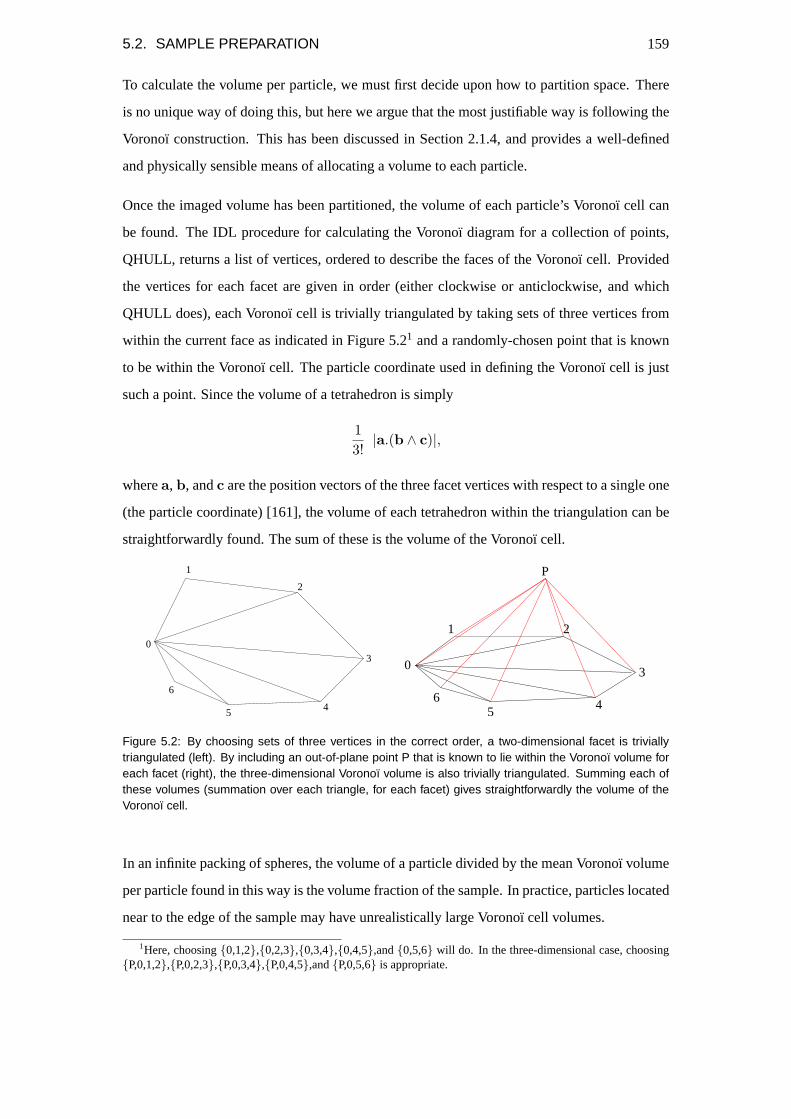
5.2. SAMPLE PREPARATION 159
To calculate the volume per particle, we must first decide upon how to partition space. There
is no unique way of doing this, but here we argue that the most justifiable way is following the
Voronoı construction. This has been discussed in Section 2.1.4, and provides a well-defined
and physically sensible means of allocating a volume to each particle.
Once the imaged volume has been partitioned, the volume of each particle’s Voronoı cell can
be found. The IDL procedure for calculating the Voronoı diagram for a collection of points,
QHULL, returns a list of vertices, ordered to describe the faces of the Voronoı cell. Provided
the vertices for each facet are given in order (either clockwise or anticlockwise, and which
QHULL does), each Voronoı cell is trivially triangulated by taking sets of three vertices from
within the current face as indicated in Figure 5.21 and a randomly-chosen point that is known
to be within the Voronoı cell. The particle coordinate used in defining the Voronoı cell is just
such a point. Since the volume of a tetrahedron is simply
13!|a.(b ∧ c)|,
wherea, b, andc are the position vectors of the three facet vertices with respect to a single one
(the particle coordinate) [161], the volume of each tetrahedron within the triangulation can be
straightforwardly found. The sum of these is the volume of the Voronoı cell.
3
5
0
6
1
2
4
0
1 2
3
456
P
Figure 5.2: By choosing sets of three vertices in the correct order, a two-dimensional facet is triviallytriangulated (left). By including an out-of-plane point P that is known to lie within the Voronoı volume foreach facet (right), the three-dimensional Voronoı volume is also trivially triangulated. Summing each ofthese volumes (summation over each triangle, for each facet) gives straightforwardly the volume of theVoronoı cell.
In an infinite packing of spheres, the volume of a particle divided by the mean Voronoı volume
per particle found in this way is the volume fraction of the sample. In practice, particles located
near to the edge of the sample may have unrealistically large Voronoı cell volumes.
1Here, choosing{0,1,2},{0,2,3},{0,3,4},{0,4,5},and{0,5,6} will do. In the three-dimensional case, choosing{P,0,1,2},{P,0,2,3},{P,0,3,4},{P,0,4,5},and{P,0,5,6} is appropriate.

160 CHAPTER 5. SAMPLE PREPARATION AND CHARACTERISATION
Figure 5.3 shows the Voronoı diagram for a random collection of points in a finite two di-
mensional region (the bounding rectangle denotes the edge of the region). Since the Voronoı
construction returns the convex hull defined by the particles, some of the Voronoı “volumes”
are in fact unbounded. These are easily dealt with, since they are identified by QHULL, and
ignored. However, for particles near to the edge of the packing, it is possible to have bounded
but still unrealistically large Voronoı volumes. Such a case is illustrated in Figure 5.3 (indicated
as Volume 2). Here, due to the proximity of the region boundary, one cannot be certain that the
apparently large region is genuine, since these are most often a result of excluded neighbours
just outside the region imaged. One must therefore be careful not to include particles which
lie “too close” to the edge of the volume: clearly this problem can be overcome by using only
particles from deep within the packing, but criteria for choosing the correct region are not ob-
vious. The selected region must be small enough to avoid this difficulty but still retain as many
particles (in the interests of maximising the statistical information) as possible.
Volume 1
Volume 2
Figure 5.3: Voronoı diagram for particles in a two dimensional region. The volume of the Voronoı cellfor a particle is its local volume fraction, provided it is in the bulk of the sample. Volume 1 in this imagecorresponds to one such particle. If a particle lies too close to the edge (Volume 2), its determinedVoronoı volume will be unrepresentatively large. See text for the resolution.
If we were to plot the distribution of Voronoı volumes without taking this into account (that is,
for all particles in the packing), we would arrive at something similar to Figure 5.4. In this, the
particles near to the edge of the image contribute to the tail of larger volumes. Note also that
missing particles, as argued earlier, will cause their neighbours to contribute to volumes in this
tail as well. If we were able to extract themost likelyvalue, ormodeof this distribution, then
we would have a reasonable estimate of the the mean volume per particle.

5.2. SAMPLE PREPARATION 161
occurrences
Voronoi volume
mean
mode
median
Figure 5.4: Illustration of how inclusion of particles which do not genuinely belong to the bulk sampleskew the distribution of Voronoı volumes. The distribution is considered suitably symmetric if the meanand median differ by less than (an arbitrary value of) 3%.
The mode of an arbitrary distribution is in general quite difficult to access, since it requires a
parameterisation of the distribution. We can arrive at a reasonable alternative: by considering
particles within a certain fraction (say30% to70%) of the maximum dimension in each direc-
tion, this distribution should become much less skewed towards larger volumes. Ultimately, in
a homogeneous sample (and assuming negligible particle misidentifications), we would expect
the distribution to be symmetric. For a symmetric distribution, the median and the mean val-
ues should coincide; indeed their difference is sometimes used as a measure of skewness. By
considering successively smaller regions from the centre of the box, the difference between the
median and the mean should become successively smaller. Once they agree to within a certain
tolerance, reasonable confidence can be had that the distribution is representative of particles
that genuinely lie within the “bulk” of the sample; this forms my definition of “in the bulk”.
Note that we do not prove the assertion that the distribution of Voronoı volumes should be
symmetric in a homogeneous sample; this is a hunch. It seems reasonable, at least, and we
have observed that using all of the particles in the packing, one achieves a distribution shaped
like that in shown in Figure 5.4. Reducing the size of the region, this tail reduces in the expected
manner as we argued should happen and the distribution becomes more nearly symmetric; we
take this as justification for our method.
In practice, the maximum difference between the median and the mean deemed permissible was
chosen to be3%. In most cases, the difference was smaller than this, although this measure
certainly has indicated problems in certain samples and therefore must be judged useful.
162 CHAPTER 5. SAMPLE PREPARATION AND CHARACTERISATION
Error in Volume Fraction from Particle Coordinates
The most basic means of means of calculating the volume fraction from the particle coordinates
is simply to divide the volume occupied by the particles by the total volume of the sample. The
volume of the particles is known (the radius of the particles and the number in the sample are
known), as is the total size of the box (the pixel pitch is known). If the number of particles
detected is different from the number in the same, or there are any “mutant” large or small
particles, then this volume fraction is no longer accurate. We do not rely on this method for
these reasons.
The method described above is much better, however, since it is not affected by either of these
problems. It is subject to statistical error, and a systematic error related to the skewness of the
distribution of Voronoı volumes. The systematic error is considered minimal, and is certainly
much less than the3% criterion detailed above.
The random error is simply due to the small size of the samples used, and can be recovered by
averaging. We have always averaged over a minimum of five datasets (except where indicated),
and this has provided an acceptably small error bound onΦ. Where error bounds are denoted
in the results, they are the standard deviation of the averaged values. In any case, we argue that
this is an improvement on the intended volume fraction.
The volume fraction is of course found by assuming the particle radius. This is subject to a
relatively large error, which introduces another potential systematic error,∆r, in Φ and remem-
bering thatΦ ∝ r3, we see that∆ΦΦ ∝ 3∆r
r . This large error (as a rough guide,∆rr '0.015, so
∆Φ'5%) goes some way to negating the advantage of this method. As it turns out, the results
are convincing.
5.2.5 Preparing Samples of Known Volume Fraction
Given a stock solution of known volume fraction, it is a straightforward matter to achieve
samples of other volume fractions which are known relatively to high precision. Martelozzo
describes this process in detail ([5]). The errors in measuring mass of added solvent can be
made very small by measuring sufficiently large quantities. In this thesis, measurement errors
were always less than1%.
For the non-density-matched samples, it is assumed that the densities of the particles and sol-
vent are accurately known. This is also discussed in [5], and there is no way of assessing how

5.3. EXPERIMENTAL EQUIPMENT 163
realistic this assumption is. Since we calculate the volume post-experiment, and find convinc-
ing agreement, we do not consider this troublesome. In the density-matched samples, there is
no such trouble. The corresponding problem here is in the inevitable slight density mismatch.
A simple web-based applet to calculate the volume fraction achieved by dilution by a known
amount of solvent of known density of a known volume fraction of particles whose density is
also known was written and has been made available online [162]. This tool helps to minimise
mistakes for these tedious calculations.
5.3 Experimental equipment
5.3.1 Sample Mountings
Microscopy of bulk suspensions places particular requirements on the sample cells. In the bio-
logical sciences, where microscopy has been an arguably much more exploited tool than in the
physical ones, there have been developed a great many methods and techniques for mounting
specimens. Even extracting thin (“two dimensional”) samples suitable for conventional mi-
croscopy requires considerable skill. Achieving “bulk conditions” by extending this to three
dimensions is a significant task.
Sample requirements for the physical sciences are typically much less difficult to achieve.
Generally speaking, there are fewer variables in addition to the control parameters whose values
are critical (for example, pH, temperature, salt concentration, ... the biologist’s life can be very
complicated in this regard). However, there are several requirements that must be met in order
to be able to image even the simplest sample.
For the purposes of colloidal studies, the sample cell required is nothing more than a chamber
into which a suspension can be placed. Finding a suitable cavity, however, is not trivial, since
it must simultaneously be:
• optically suitable, so that the suspension can be imaged.
• airtight , for at least as long as the experimental timescale, but ideally for much longer
than this.
• straightforwardly filled and then sealed, so that there is minimum solvent loss during
this process. Additionally, the process must be such that the sample does not come into
164 CHAPTER 5. SAMPLE PREPARATION AND CHARACTERISATION
contact with any substance which may alter its behaviour.
• impervious to the constituents of the sample, so that the sample can exhibit its genuine
bulk behaviour and not reflect the properties of the cell.
Mark Elliot [57] described in detail the optical requirements of a sample cell suitable for col-
loidal studies. Though designed for conventional microscopy, his discussion remains valid;
there is, however, a significant simplification that arises when the cells are to be used for con-
focal microscopy. Since the confocal microscope uses only one lens which serves as both the
objective and condenser lens, only one wall of the sample cell need be optically suitable. Opti-
cally suitable means [57] here that the thickness of this wall must be suitably thin. For further
details on general requirements on microscopical observation cells, please see [57]. Here, all
that really matters is that the coverslip is correct thickness.
Whilst easy to manufacture, the cells described by Elliot were found not to give particularly
good images. No reason was immediately obvious for this, other than that their walls are not
the standard170µm thickness for which the objectives are corrected. More probable is that the
walls of the capillary tube, which are not designed primarily for microscopy, are not suitably
optically flat. As Elliot points out, immersion oil that is index-matched with the capillary tubes
will negate the effect of surface relief. However, any imperfection within the tube walls may be
detrimental to their optical properties. The method of production of these particular capillary
tubes is not known, but it is likely that they are drawn from molten glass as are other tubes (see,
for example, [163]). It may be imagined that this process introduces heterogeneities which
could explain their poor optical properties. It should be noted that this is mere speculation, and
that the cause of the poor performance was not investigated.
Several experiments suggested, as one might expect, that standard microscope cover glasses
provided much superior images to those obtained using the capillary tubes. For this reason, it
was decided to design a sample cell that had one of these as the wall through which imaging
takes place. In fact, in this investigation, two cells were developed. The first is a robust, well-
sealed and appealing cell, but which is only really suitable for fluid samples. The second is less
well made and cannot reliably be used over many months, but is appropriate for even the most
dense colloidal samples.

5.3. EXPERIMENTAL EQUIPMENT 165
5.3.2 Sample Cell 1
The first cell developed has a cover slip for its imaging side (the base, usually, since an inverted
microscope was used here). The remaining design considerations are in the remainder of the
cell (the “top”) and how it will be attached to the coverslip. The top of the cell is illustrated
in Figure 5.5. In principle, this could be crafted from any material. In practice, they were
machined from readily available sheets of perspex (PMMA) available as surplus in the Physics
workshop. These sheets are of variable thickness even within a single sheet, so were machined
flat. The thickness requirement (3–4mm) is not critical; it is a convenient amount that is both
large enough to permit suitable sample depth (∼ 100µm) and to give the cells considerable
mechanical strength. It is also the most commonly available thickness of perspex sheet.
=0.6mmΦ
10
3−4
22
50
25
cavity 0.5mm
Figure 5.5: Dimensions of the top of sample cell 1. The cavity boundary usually has rounded edges forease of manufacture (see text).
The cell represented here is as large as is reasonably practicable, since the largest readily-
available cover glasses are22mm×50mm. Sometimes, a smaller sample cell may be required
(for example18mm×18mm) to, for example, fit into a centrifuge tube. This is a straightforward
modification, since all of the length measurements indicated here can be adjusted as required.
Naturally, the cavity must have suitably thick walls for machining reasons (and so that the cover
glass can be attached), but in practice this limit maintains a sample volume that is much larger
than is ever required.
The exterior of the cell can be machined to high precision by milling. The boundaries of the
cavity can be created to similar precision, but due to the shape of the tip of the milling bit,
the cavity is not of uniform depth. With experience and care, these can be minimised, but
are still clearly present. For this reason, the cavity was typically cut to a greater depth than
was necessary, so that the effect of surface imperfections could be assumed to be unimportant.
Additionally, whilst it is possible to mill a rectangular cavity, in practice it is more straightfor-

166 CHAPTER 5. SAMPLE PREPARATION AND CHARACTERISATION
ward to leave rounded corners (since the milling bit is approximately cylindrical). This was not
considered a problem and was routinely done.
The volume of the cavity can be adjusted as indicated above, but is typically in the range
20µl–125µl (for 10mm×10mm×0.2mm and25mm×10mm×0.5mm cavities respectively).
Assembling the Cell
Assembling the cell is essentially straightforward, requiring only a cover glass of appropriate
size to be glued to the perspex cavity. Before assembly, the components are washed in a
standard laboratory detergent solution, Decon 90 (Decon Laboratories Limited,
http://www.decon.co.uk/english/index.htm), either being left overnight, or placed in a sonicator
for at least 15 minutes. They are then rinsed in deionised water and dried in an oven at' 50 ◦C.
A suitable adhesive must be chosen. Norland Products Inc. (http://www.norlandprod.com/)
produce a range of UV-cure adhesives, which set only on exposure to ultraviolet light. It was
found here that Norland Optical Adhesive (NOA) 61 was suitable. The top (perspex part) of the
cell is placed topside-down on the bench and adhesive applied to the surface to which the cover
glass is to be affixed. This is achieved using a pneumatically-operated syringe (EFD Model
Number 1000DVE, http://www.efd-inc.com/) which delivers glue at a constant, controllable
rate via32 gauge,14′′
length tips (Part Number: 5132-1/4-B). Since it does not set until cured
with UV, this operation is straightforward. The adhesive is applied in a similar fashion to
that illustrated in Figure 5.6. The lines represent “beads” of adhesive that become squashed
to achieve more-or-less full coverage of the surface as the cover glass is depressed onto the
surface. Achieving a uniform thickness of adhesive, including up to the edges, is very nearly
possible with practice. A cell will be airtight provided the adhesive percolates the sealed area;
a visual inspection can confirm satisfactorily whether this is the case.
Once the cover glass has been firmly pressed onto the surface, the cell is positioned under a
UV lamp (UVP Inc., http://www.uvp.com/new/) model “Blak-Ray”, B-100A, which produces
8900µW/cm2 at a distance of10′′ (http://uvp.com/new/index.php?module=ContentExpress&
func=display&ceid=90), and left to cure. The process takes around half an hour, though this
time is not critical [164]. The glue will ultimately cure in ambient light to anneal imperfections,
and secondary reactions continue to take place for around 24 hours [165]. Sample cells are
therefore left for around a day before being filled. It is worth noting that the UV lamp required
for this purpose is relatively low-powered and requires minimal precautions for the user.

5.3. EXPERIMENTAL EQUIPMENT 167
cover glass
Figure 5.6: Adhesive is applied in uniform tubular “beads”, such that coverage is as near-uniform aspossible once the cover glass is pressed into place.
Filling the Sample Cell
The design of the cell is such that once the cover glass has been attached, the sample chamber
is still exposed to the outside world by the two0.6mm drill holes through the cell. One of these
is intended to allow the cell to be filled, the other a “breather” that permits the chamber to be
evacuated of air as the sample is injected. It has been found by experimentation that the cell
is easier to fill if the holes are well separated. To fill the chamber, a1ml disposable syringe
(BD Plastipak JM990R, www.bd.com) is fitted with a23 gauge (0.6mm) number16 needle
(BD Microlance 3 Luer JN010R, www.bd.com) and filled with the sample. The syringe is then
evacuated into the chamber using the filling hole. When filling and evacuating the syringe, as
little pressure as possible is used to minimise the possibility of particles jamming due to the
confining geometry. The cell can be tilted to facilitate the evacuation of air.
As shortly as is reasonable after this procedure, each of the holes is sealed in the same way as
the other, with a generous “dollop” of two-part epoxy resin (Araldite). It is useful, although
sometimes difficult, to avoid the two lumps of epoxy from merging, since a small visible win-
dow can be useful for preliminary conventional microscopy of the sample. (In this design the
optical properties of the top surface are not ideal. A perfect cell for conventional microscopy
could be manufactured with a cover slip on one side and a microscope slide on the other.) The
epoxy is then left to dry. The seal so created is absolutely solvent-tight for at least a period of
several months, and in fact samples of considerably over a year old show no signs of solvent
evaporation.

168 CHAPTER 5. SAMPLE PREPARATION AND CHARACTERISATION
Cell Discussion
The sample cell described above meets well the numerous constraints set out above. In partic-
ular, and most importantly, it provides excellent image quality owing to its cover glass base.
It is made of glass and PMMA, which are suitable materials for containing the samples used
in this enquiry. The UV-cure adhesive bonds the cell together well enough that samples last
for at least one year apparently unscathed (and therefore must seal effectively perfectly, since
a similar-sized sample dries overnight if exposed to the atmosphere). Additionally, this adhe-
sive has been used by other groups to their satisfaction for some time [166], as well as our
own group. The epoxy resin used here has been widely used and found to be satisfactory [57].
Finally, if made carefully, the cells, are suitable for qualitative imaging with a conventional
microscope. This should not be overlooked as an advantage, since it is frequently easier to
identify colloidal particles in a conventional rather than confocal microscope.
These cells are rather time-consuming to produce, and it is only recommended that they be used
in circumstances where quantitative analysis is a requirement. Otherwise, the capillary tube
mountings may suffice. A more compelling difficulty is that they are filled via a narrow channel
using a syringe. Such a constriction is very difficult to force dense samples through. Practical
experience suggests that samples of volume fraction greater than around60% are extremely
difficult to pass through a syringe, becoming practically solid. This is perhaps unsurprising,
given that Haw [159] has observed apparent jamming of colloidal suspensions as they are
handled by syringe.
A last comment regarding this method of filling is somewhat more speculative, but nevertheless
it may be relevant. It has been reported that imposed shear flows on colloidal suspensions cause
crystallisation (see for example [160]). It may be that forcing a suspension into a cell with a
parallel geometry in this way could cause crystallisation. This has not been observed so far,
but is perhaps worth bearing in mind.
5.3.3 Sample Cell 2
The second type of cell used here is appropriate for almost all samples, no matter how dense.
It is extremely simple by comparison with the previous cell. Figure 5.7 (left) illustrates a small
glass vial which forms the basis of the cell. The centre image in this Figure shows the same
vial, having had its base cut off, being glued using the same UV-cure glue as above to a cover

5.3. EXPERIMENTAL EQUIPMENT 169
slip of the correct thickness. Once the glue has cured, the sample is placed in the cell and the
threads wrapped carefully with Teflon (PTFE) plumbers’ tape. The lid is placed onto the vial,
and this is wrapped carefully with standard laboratory sealing film (Parafilm).
=⇒����������������������������
����������������������������
���������������
���������������
=⇒
Figure 5.7: The second type of cell consists of a typical small glass vial (left) having its base removedand being glued to a suitable cover slip (centre). The completed cell is filled and sealed with PTFE tapeand Parafilm.
These cells have the advantage that they can be filled with denser samples, and that they are
substantially easier to make. They do not, however, seal perfectly as reliably as the other cells,
but do seal sufficiently well enough for most experiments.
5.3.4 Oil Immersion
As described in Section 3.2.2, the diffraction limit of the imaging system is governed by the
numerical aperture of its lenses. In the confocal case, in practice this means that the resolution
(explicitly, the extent of the point spread function) is primarily determined by the objective
lens used. Mark Elliot’s PhD thesis describes nicely the oil immersion technique [57,§2.3.5],
and all of what he says is well written and applies here. We make a further remark about the
refractive index of the sample itself.
To achieve the best possible resolution for a given wavelength of light requires as high a nu-
merical aperture as possible. Figure 5.8 is a schematic illustration of the front of an objective
lens receiving light. The left-hand image illustrates the situation in the case where there is
simply an air gap between the cover slip and the objective. Since the cover slip has a refractive
index higher than that of air (ncs'1.50, c.f. nair=1), there is refraction at the interface; this
results in a reduced refractive index and therefore worse resolution than were the light rays
undeviated. This also has the disadvantage of reducing the light budget to the objective lens,
which leads to less bright images. The numbers in this example are realistic, but are quoted
without justification; for more detail, see [57,§2.3.5] and [106, also§2.3.5].
This problem can be addressed by reducing the difference between the refractive indices and
therefore the amount of refraction at the air-coverslip interface. This could in principle be

170 CHAPTER 5. SAMPLE PREPARATION AND CHARACTERISATION
achieved by reducing the refractive index of the coverslip, though no useful material comes
close to having a sufficiently low refractive index. Furthermore, the sample itself is of an es-
sentially non-negotiable refractive index, and since a similar argument applies at the coverslip-
sample boundary, ideally we desire to match the refractive indices of the sample, coverslip, and
the medium between the coverslip and the objective lens.
cover slip
oil
39
72 air
68
front lensobjective
Figure 5.8: A schematic of the effect of an oil immersion lens. The angle of the light cone entering theobjective lens does not change significantly, but the increased refractive index of the immersion oil overair permits a much larger numerical aperture.
Figure 5.8 (right) shows how a droplet of oil applied to the objective lens can help. It shows the
case where the coverslip and the oil have exactly the same refractive index, so that refraction
has been wholly eliminated. Here, although the angle of the light cone entering the lens has
slightly reduced, the numerical aperture (which is given byA′ = n′ sinσ′) has increased from
1× sin(72) = 0.95 to 1.51× sin(68) = 1.40, for a typical immersion oil.

Chapter 6
Bridges
We devote this Chapter to discussing in detail the technique used to find bridges. We discuss
what a bridge is, and what it requires in three dimensions. This involves explaining how spheres
can be stabilised against gravity by one another in three dimensions, and how cooperative
stabilisations are vital. Crucial in this is identifying contacting neigbours, which is non-trivial.
We discuss the basic results, as well as the necessary parameter choice and assumptions we
must make.
The definition of a bridge used here is the same one used by Barkeret al. [95, 96]. It is
intuitively appealing, and quite straightforward.
6.1 Identifying bridges
The algorithm used for finding bridges is very simple, but can result in complex bridge geome-
tries. We start by considering what is meant by a bridge, and it turns out that all bridges, no
matter how complex, arise as a result of two requirements. We discuss these by considered the
familiar humpback road bridge, Figure 6.1.
What makes a bridge?
It is intuitively clear that every constituent component (stone!) of a bridge is prevented from
falling under the influence of gravity: every stone isstabilised, or supported. This is the first
necessary property of a bridge. To be considered a bridge, however, the collection of stones
must also act cooperatively so that all but the end stones are not supported by the ground.
171

172 CHAPTER 6. BRIDGES
Figure 6.1: A familiar humpback bridge. This is the Ross Bridge over the River Earn at Comrie,Perthshire, built in 1792.
We discuss these two properties specifically for the case of spherical particles. We then outline
the algorithm used to search for instances of these criteria being met, and show that these alone
give rise to complex bridge geometries.
6.1.1 Stability criterion for spherical particles
The process of bridge finding begins by identifying which particles are stable, since only these
can belong to a bridge. It is worth noting that it is possible to find unstable particles in dense
packings of spheres, even at very high densities. In random packings, it is believed possible
even up to around the MRJ (maximally random jammed) density (Chapter 2), via “rattlers”. In
crystalline solids, it could in principle occur until very near to the close-packed limit of74%,
since particles are only forced into contact at this point.
Figure 6.2 (left) illustrates the simple condition for a spherical particle to be stabilised in two
dimensions. At least two touching neighbours are required to support each stable particle, and
in order to be stable, they must be arranged so that theweight vector of thecandidate stable
particle (the uppermost, in this case) passes directly through the line of centres of the two
stabilising or baseparticles. The weight vector is simply a vector pointing in the direction of
the applied force. Its magnitude is not important in determining whether it crosses the line of
centres (i.e. if necessary, it is extended).
Figure 6.2 (middle) shows a simple example of an arrangement of particles in which, although
the candidate stable particle has two touching neighbours, they are arranged so that its weight
vector does not pass through their line of centres. In this case, it is clear that the particle is not
stabilised by these two particles and will tend to roll off in the direction indicated by the arrow
unless supported by further particles in the packing.
Figure 6.2 (right) shows another set of three particles. In this instance, the middle particle is

6.1. IDENTIFYING BRIDGES 173
Figure 6.2: In two dimensions, a stable particle (left) and an unstable particle (middle). The rightmostfigure illustrates the important point that the centre of mass of the supported particle need not be higherthan those of the supporting particles.
stabilised by the two base particles. This makes the important point which also applies in three
dimensions that, unlike in the intuitive case shown in Figure 6.1, the centre of mass of a base
particle can be higher than the centre of mass of the supported particle.
Figure 6.3: Even in two dimensions, a stable particle can be stabilised by more than one subset. Here,the blue particles and the red particles both give support to the green one independently.
The last important point relating to the stability of particles is that even in two dimensions there
can be more than onestabilising subsetper stable particle. Figure 6.3 shows a stable particle
with four stabilising particles arranged into two stabilising subsets. This represents redundancy
in the stabilising network of forces and will be investigated later.
Three dimensions
In three dimensions, the criterion is a simple extension of the above. Figure 6.4 shows that a
candidate stable particle requires at least three contacting neighbours to be stabilised. In this
case, the weight vector must pass through a triangle whose vertices are the centres of the base
particles. Once again, one or more of the base particles can be higher than the stable one, and
there can be more than one stabilising subset.

174 CHAPTER 6. BRIDGES
Figure 6.4: The criterion for stability in three dimensions. Three particles provide stability to a fourth if itsweight vector passes through the triangle formed by the vertices of the three supporting particles. In thisimage, the particles have been reduced in size for clarity; in fact, they are contacting neighbours.
6.1.2 Identifying cooperative stabilisations: mutual stabilisations
Once each particle in a given packing has been deemed stable or otherwise, one can identify
whether there are any cooperative effects which give rise to non-trivial bridges. The necessary
cooperative behaviour is referred to asmutual stabilisation.
Mutually stabilising particles
Figure 6.5 shows a cartoon of a humpback bridge similar to the one shown in Figure 6.1; we
use this to illustrate the concept of mutual stabilisation. In this, the “base particles” are the two
abutment “stones” labelled1 and7. These are base stones because they rely on no other stones
in the bridge for stability. The remaining stones all rely on other stones for their stability. For
1
2
34
5
6
7
Figure 6.5: A cartoon of a humpback bridge, in which particles 2, 3, 4, 5, and 6 are involved in mutualstabilisations.
example, the keystone, stone4, relies on stones3 and5 for its stability. Stone3, however, is
stabilised by stones2 and4. This means that removing stone3 would cause stone4 to fall, but
that equally removing stone4 would cause stone3 to fall. That is, stones3 and4 are mutually
stabilising. In this example, stones2, 3, 4, 5, and6 are all involved in mutual stabilisations. We
use this to establish the convention that only those particles involved in mutual stabilisations
are considered to be members of the bridge.
Figure 6.6 (left) illustrates a two-dimensional2-particle (i.e. minimal) bridge. In this, particles
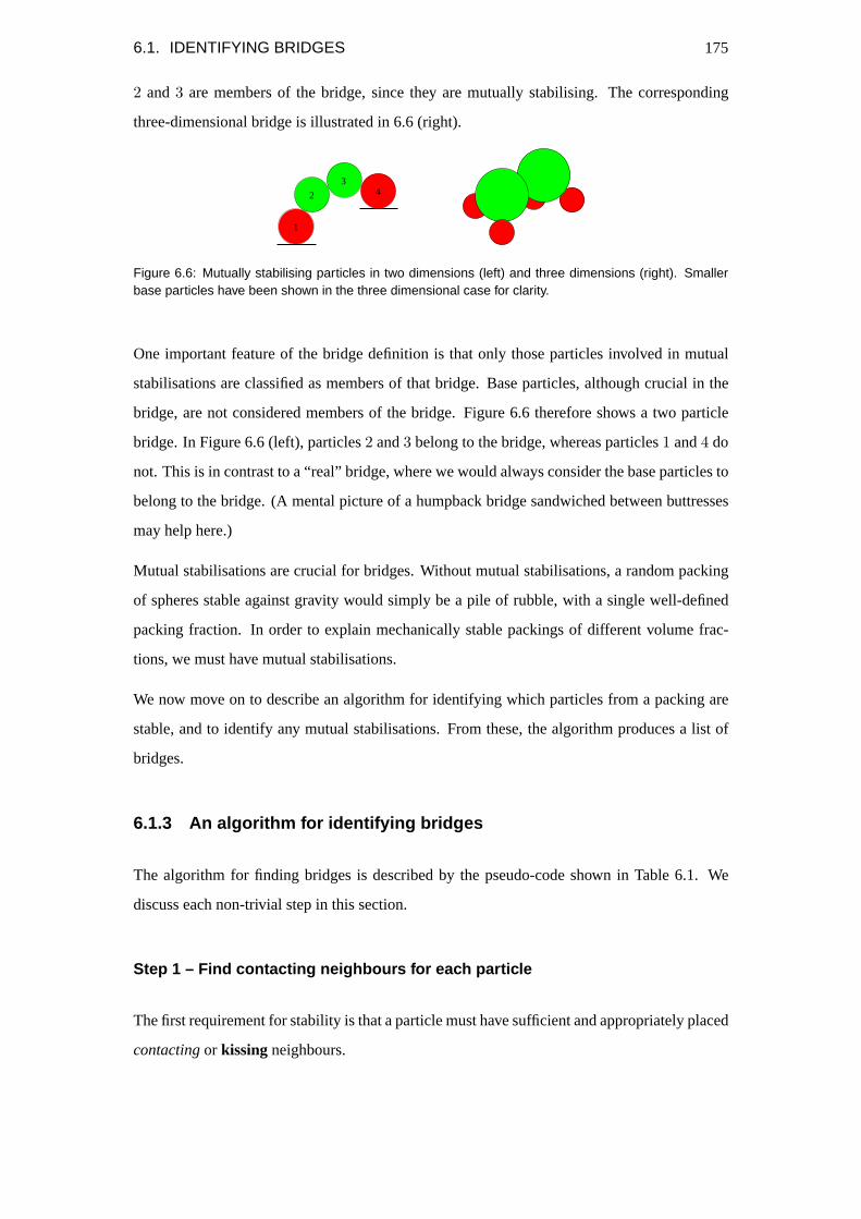
6.1. IDENTIFYING BRIDGES 175
2 and3 are members of the bridge, since they are mutually stabilising. The corresponding
three-dimensional bridge is illustrated in 6.6 (right).
1
2
34
Figure 6.6: Mutually stabilising particles in two dimensions (left) and three dimensions (right). Smallerbase particles have been shown in the three dimensional case for clarity.
One important feature of the bridge definition is that only those particles involved in mutual
stabilisations are classified as members of that bridge. Base particles, although crucial in the
bridge, are not considered members of the bridge. Figure 6.6 therefore shows a two particle
bridge. In Figure 6.6 (left), particles2 and3 belong to the bridge, whereas particles1 and4 do
not. This is in contrast to a “real” bridge, where we would always consider the base particles to
belong to the bridge. (A mental picture of a humpback bridge sandwiched between buttresses
may help here.)
Mutual stabilisations are crucial for bridges. Without mutual stabilisations, a random packing
of spheres stable against gravity would simply be a pile of rubble, with a single well-defined
packing fraction. In order to explain mechanically stable packings of different volume frac-
tions, we must have mutual stabilisations.
We now move on to describe an algorithm for identifying which particles from a packing are
stable, and to identify any mutual stabilisations. From these, the algorithm produces a list of
bridges.
6.1.3 An algorithm for identifying bridges
The algorithm for finding bridges is described by the pseudo-code shown in Table 6.1. We
discuss each non-trivial step in this section.
Step 1 – Find contacting neighbours for each particle
The first requirement for stability is that a particle must have sufficient and appropriately placed
contactingor kissingneighbours.

176 CHAPTER 6. BRIDGES
1. Find a list of contacting neighbours for each particle
2. Establish which particlescouldbe stabilised
3. FOR each particle DO
4. Establish which, if any, subsets of particles stabilise that particle
5. END FOR
6. Extract one only of the stabilising subsets for each particle
7. Identify any mutual stabilisations
8. Group mutual stabilisations into clusters, to find bridges
9. Output results
Table 6.1: Pseudo-code for Bridge Finder main program.
Smart (and efficient) algorithms assign neighbours on more sophisticated criteria than sim-
ply separation distance. In particular, the Voronoı tessellation is useful in uniquely assigning
neighbours efficiently 2.1.4. However, this is not necessary, and neighbours were found using
a criterion based on the separation of particle centres.
To classify particles as contacting for monodisperse spheres whose centres are known to ma-
chine precision is easy: if the positions of two particlesi andj areri andrj , then two particles
are kissing neighbours if and only if|ri−rj |2−σ2 ≤ ε2 , whereε is the appropriate machine
precision andσ is the particle diameter.
For real colloidal particles, the situation is complicated by the polydispersity of the particles,
as well as the error in the coordinates. Figure 6.7 shows that in the case of different sized
particles, the condition becomes|ri−rj |2−(
σi+σj
2
)2≤ ε2. Although in principle one could
allow for this, in this thesis the radius of each particle was never known to a suitable level of
accuracy, and therefore a mean value was used throughout.
i jσ σ
σ σ+i j2
Figure 6.7: In the case of polydisperse particles, the separation of centres is different for each pair ofparticles.

6.1. IDENTIFYING BRIDGES 177
Figure 6.8 illustrates the problem due to inaccuracy in the particle coordinates. This case is the
common error argued in 4.6, where particle centres have been found to be too close together.
In fact, for the purposes of finding contacting neighbours, this is tolerable, since we can use
the criterion|ri−rj |2 ≤ σ2 (Strictly, |ri−rj |2 ≤ (σ+ε)2, but ε¿σ). In this case, any particle
centres which are closer than the mean particle diameter are considered kissing neighbours.
< σ
Error in coordinate
Figure 6.8: For particles whose centres are too close together, the condition for kissing neighbours isaltered, but still captures
The real problem arises when the centres are found to be too far apart, in which case particles
which are genuinely contacting would not be counted as such. In this case, to be certain of
finding all neighbours, one must count a particles neighbours as being all of those for which
the condition|ri−rj |2 ≤ c2 is true, wherec is acutoff value which is larger than the particle
diameter.
Both polydispersity and inaccuracy in the particle coordinates mean that the cutoff parameter
used to define a particle’s neighbours must be larger than the diameter. A suitable value must be
determined by experimentation, but we may make an estimate of using the following argument:
If the polydispersity of the particles lies somewhere in the range5-10% 2.2.3, and the error in
the coordinates is around50nm, i.e. ' 5% (assuming an isotropic resolution), then we may
expect that the appropriate cutoff value be around7% (=√
(52 +52)) to 11% (=√
(102 +52))
larger than the diameter. That is,c = 1.07-1.11σ. It is clear that in many cases this will classify
as neighbours particles which are not actually touching, but this is a necessary penalty for being
certain to have captured all genuine contacts. A compensation for this overcounting will be
considered later.
Step 2 – Establish which particles could be stabilised
For real data, unlike in simulations, the finite box size means that some particles cannot be
stabilised. Rather than taking advantage of periodic boundary conditions, for experimental

178 CHAPTER 6. BRIDGES
4.1. IF current particlecouldbe stabilised then DO
4.2. IF current particle has3 or more neighbours then DO
4.3. Find stabilising subsets from these neighbours
4.4. IF there is at least one stabilising subset then DO
4.5. Add current particle and its stabilising subsets to list
4.6. END IF (4.4)
4.7. END IF (4.2)
4.8. END IF (4.1)
Table 6.2: Pseudo-code for Bridge Finder Step 4.
data there is simply no data available for the neighbours whose centres lie within one particle
diameter of the edge of the dataset.
To allow for this, each particle in the dataset must be assessed to decide whether it could be
stabilised. Since the particle location algorithm results in the loss of information of a border of
a certain width (in the case of SSFrefine, this border is of width one particle diameter 4.7), the
particles which could be stabilised lie within a “double border”. The appropriate condition for
the potentially stable subset of particles is then the width of the feature border plus the particle
radius. In most of the datasets used in this thesis, the total border width was32σ.
Step 4 – Establish stabilising subsets for current particle
Table 6.2 shows a pseudo-code representation of the task of establishing whether a particular
particle is stable, and, if it is, the identities of those particles which stabilise it. Step 4 regards
what is done if a particle is potentially stable, that is, if it falls within the subset of particles
which could be stable, as defined in Step 2.
In Step 4, the first task is to establish whether the current particle could be stabilised in prin-
ciple. This is a test to find out whether it is a position in the sample where its neighbours
could provide support. In practice, this means it must be at least one diameter from the edge
of the dataset. If it is closer to the edge than this, then it may be stabilised in reality by parti-
cles which the particle tracking does not adequately detect, and therefore will be inaccurately
declared unstable by the analysis.
If the current particle lies in such a position in the sample that it could in principle be stable,

6.1. IDENTIFYING BRIDGES 179
then its neighbours are tested to see if they can provide stability.
Testing a particle’s neighbours for stabilising subsets
It is not sufficient here simply to establish whether any set of three neighbours provides support
to the current particle; we are interested in all of the stabilising subsets. For this reason, we
must testeverypossible set of three neighbours. This is a fairly straightforward combinatorial
problem. If we have four particles, labelled1, 2, 3, 4, then the possible combinations are:
1 2 3
1 2 4
1 3 4
2 3 4
Similarly, for five particles, the possible combinations are:
1 2 3
1 2 4
1 2 5
1 3 4
1 3 5
1 4 5
2 3 4
2 3 5
2 4 5
3 4 5
It follows from these patterns that forN particles, there areNC(N−3) (or equivalently,NC3
subsets of three particles. In principle, any of these could be stabilising (though not all together,
presumably, due to the packing constraints).
Checking for Stability
We test each potentially stabilising subset in turn, using the following method.
Firstly, the three members of the candidate stabilising subset are extracted and their coordinates
used to define the three vertices of a triangle. This triangle lies in a plane. The weight vector of

180 CHAPTER 6. BRIDGES
the particle is found by extending a line from the centre of the candidate stable particle directly
downwards to a point with the same x- and y-coordinates, and the coordinate z= 0.
It is a straightforward geometrical task to then determine if this weight vector intercepts the
triangle (the necessary condition, see Figure 6.4). A nice implementation of an algorithm to do
this is available from [167]; we describe it briefly here.
Firstly, we check that the weight vector is not parallel to the plane in which the triangle lies. If
it is not, we determine the point of intersection of the line with the plane. The intersection point
must also lie within the weight vector, rather than just somewhere along the line of which it is
a segment; this could occur if the potentially stabilising set of three particles formed a triangle
above the particle, that is, it would be stable against an upward force). Lastly, the intersection
point must lie within the facet. This is easy to test; the angles between the position vectors of
the three vertices of the triangle with respect to the point of intersection should sum to2π. If
they do not, then the point of intersection does not lie within the triangle, and the particle is not
stable.
If all of the above conditions are met, then that subset provides stabilisation to the current
particle.
Steps4.4-4.6 add the current particle and its stabilising particles to a full list of stable particles.
Once the algorithm has finished, the first few entries in this list will look like that shown below.
1 2 3 4
1 2 8 5
1 6 4 5
2 1 6 7
2 6 8 9
4 5 6 10
... ... ... ...
In this list, the first column denotes the index of the particle, while the remaining three columns
contain the indices of the stabilising particle. In this case (concocted for illustrative purposes
only), note that particle number1 has three stabilising subsets, while particle3 is not stabilised
by any.
6.1. IDENTIFYING BRIDGES 181
Step 6 – Extract a single stabilising subset for each particle
We said earlier that the bridge definition permits only one stabilising subset per stable particle.
Whether this is sensible will be considered later; however, to proceed for now we need accept
that this is necessary, and decide on a rule for deciding the “best” stabilising subset to keep.
The decision of which stabilising subset to keep is not straightforward, since it is not clear
why any one should be better than any other. However, there are two clear options which are
considered in this thesis to be the obvious choices.
The first follows what Gary Barker and others do, but which is not detailed in their papers.
Since they have generated packings by allowing particles to “fall” under the influence of gravity
until stabilised, they know for certain which subset of three particles provided stability in the
first place. As we argue shortly, this does not preclude the possibility of further stabilisations
(essentially by chance, in these cases).
Barkeret al. do not require to carry out Steps1-6 for their data, since they have by construc-
tion a list of stable particles and their stabilising subsets. However, they claim ([168]) that
when they disregard this information and perform the algorithm as detailed here, there is a
close correspondence between their “real” stabilising subsets and the one of the several candi-
date stabilising subsets with thelowest centre of mass, or LCOM . This seems a reasonable
statement, since it is intuitively appealing that a stabilisation similar to that shown in Figure
6.2(left) (though in three dimensions) is “more stabilising” than one similar to that shown in
Figure 6.2(right). This is, however, an unfounded assertion and it is not clear why one should
disregard apparently good stabilisations on this basis.
In the case of arbitrarily accurately known coordinates, the LCOM method of choosing a sta-
bilising subset is as justifiable as any. Once the detrimental effects of polydispersity and uncer-
tainty in the particle locations are taken into account, it is less clear that this is the best option.
Rather, it would seem reasonable to assess the likelihood of the stabilising subsets based on
how likely all of the particles in each are likely to be genuinely contacting. The crudest method
of doing this was followed: the subset whose members were on average closest to the stable
particle was taken as being the “real” stabilising subset. This choice will be referred to as
LSSQ (lowest meanseparationsquared).
These two criteria for choosing the most likely stabilising subset are very crude. It seems
reasonable that LSSQ is likely to more nearly represent the “real” stabilisation in real samples,

182 CHAPTER 6. BRIDGES
on the grounds given above. One may be tempted to develop more sophisticated schemes
to identify the best stabilising subset in any situation. For example, one could use structural
analysis tools to assess which would bear the largest portion of an arbitrary load applied in
the direction of gravity. However, indeterminacy in the force network is a real phenomenon
in static sphere packings (e.g. granulars), and it there seems little point expending substantial
effort to perform the task of selecting one particular stabilisation, when it is known not to be
like this in reality. Rather, we accept the current approximation and see what follows.
Once we have made the decision of which stabilising subset to choose, the full list of stable
particles and their stabilising triplets will look something like the following:
1 2 8 5
2 1 6 7
4 5 6 10
... ... ... ...
This list contains all of the necessary information for determining stability, and indeed for
extracting bridges. Step7 reveals how to search this list for mutual stabilisations.
Step 7 – Identify any mutual stabilisations
Identifying mutual stabilisations is straightforward. A mutual stabilisation occurs when a par-
ticle is stabilised by a second particle, which itself is stabilised by the first.
An equivalent way of stating this condition is the following: if particlex has particley in
its stabilising triplet, then these two particles are mutually stabilising if and only if particle
x appears in particley’s stabilising triplet. In the example above, particle1 is stabilised by
particles2, 8, and5. Since particle1 appears in particle2’s stabilising triplet, we know that
particles1 and2 are mutually stabilising. It may be that particles8 and5 are also both mutually
stabilising with particle1, but we do not have information on their stabilisations.
The output from this step is a list of pairs of mutually stabilising particles:
1 2
... ...

6.1. IDENTIFYING BRIDGES 183
Step 8 – Group mutual stabilisations into clusters
To identify bridges, we group mutual stabilisations into disjoint clusters. By doing this, we
ensure that all mutually stabilised particles belong to only one bridge, but that all such particles
are counted in a bridge.
There are a number of algorithms used to generate clusters in this way. Here, the algorithm of
[169] was used, as suggested in [95]. This is a particularly neat algorithm; for a full description,
consult the original paper. What follows paraphrases the relevant part of this paper.
In the Stoddard paper, clusters are defined by a separation criterion. Here, this criterion is
replaced by whether two particles appear together in the list of mutual stabilisations. A cluster
C is a cluster if and only if it has the properties (for two particlesi andj)
1. If i ∈ C andi andj appear together in the list of mutual stablisations, thenj ∈ C.
2. If A is any set satisfying 1. above, and ifi is in bothA andC, thenA ∩ C = C.
The first property simply says that if particlei belongs to a given bridge, and particlej is
mutually stabilising withi, then particlej also belongs to that bridge.
The second property simply says that ifA is one particular bridge and particlei belongs to both
it and another bridge,C, then in factA andC are the same bridge. This is their way of saying
that a cluster consists of one disjoint (their term, for our purposes “separate” will do) group of
particles.
The second property ensures that a clusterC consists of only one disjoint group. This definition
also ensures that each particle belongs to exactly one unique cluster.
A brief aside: an example of the clustering algorithm
Clusters are stored in a one-dimensional array,L, of sizeN , for N particles. L contains
disjoint, circular sublists, with each sublist containing the members of a disjoint cluster. The
algorithm works as follows:
Initially, the entries ofL are given their indices as entries:
L = 1 2 3 4 5 6 7 ... N (6.1)
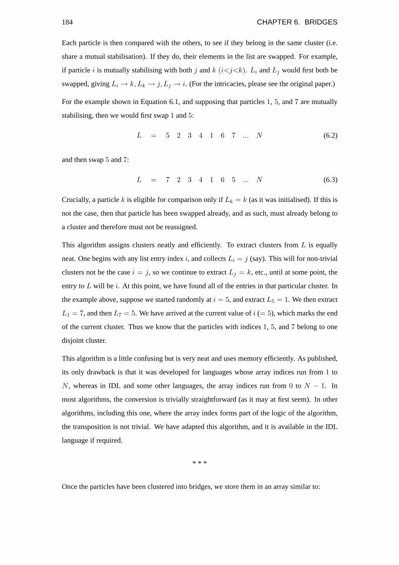
184 CHAPTER 6. BRIDGES
Each particle is then compared with the others, to see if they belong in the same cluster (i.e.
share a mutual stabilisation). If they do, their elements in the list are swapped. For example,
if particle i is mutually stabilising with bothj andk (i<j<k). Li andLj would first both be
swapped, givingLi → k, Lk → j, Lj → i. (For the intricacies, please see the original paper.)
For the example shown in Equation 6.1, and supposing that particles1, 5, and7 are mutually
stabilising, then we would first swap1 and5:
L = 5 2 3 4 1 6 7 ... N (6.2)
and then swap5 and7:
L = 7 2 3 4 1 6 5 ... N (6.3)
Crucially, a particlek is eligible for comparison only ifLk = k (as it was initialised). If this is
not the case, then that particle has been swapped already, and as such, must already belong to
a cluster and therefore must not be reassigned.
This algorithm assigns clusters neatly and efficiently. To extract clusters fromL is equally
neat. One begins with any list entry indexi, and collectsLi = j (say). This will for non-trivial
clusters not be the casei = j, so we continue to extractLj = k, etc., until at some point, the
entry toL will be i. At this point, we have found all of the entries in that particular cluster. In
the example above, suppose we started randomly ati = 5, and extractL5 = 1. We then extract
L1 = 7, and thenL7 = 5. We have arrived at the current value ofi (= 5), which marks the end
of the current cluster. Thus we know that the particles with indices1, 5, and7 belong to one
disjoint cluster.
This algorithm is a little confusing but is very neat and uses memory efficiently. As published,
its only drawback is that it was developed for languages whose array indices run from1 to
N , whereas in IDL and some other languages, the array indices run from0 to N − 1. In
most algorithms, the conversion is trivially straightforward (as it may at first seem). In other
algorithms, including this one, where the array index forms part of the logic of the algorithm,
the transposition is not trivial. We have adapted this algorithm, and it is available in the IDL
language if required.
* * *
Once the particles have been clustered into bridges, we store them in an array similar to:

6.1. IDENTIFYING BRIDGES 185
1 4 3 16 17 22 21 −99 −99 −99
2 7 5 6 12 13 23 43 32 49
8 15 24 16 19 38 20 −99 −99 −99
31 42 9 −99 −99 −99 −99 −99 −99 −99
... ... ... ... ... ... ... ... ...
(Note that here, an entirely new set of particles has been concocted to illustrate the point.) This
array has a row for each of the bridges, and as many columns as the largest bridge has members.
The entries “-99” are null values to take up space for those bridges with fewer members than
the largest bridge. This involves substantial waste of memory, and is something of an insult to
the efficiency of the clustering algorithm, but is the simplest solution and more than adequate
for the task.
Step 9 – Output results
Lastly, we must output the results. A full description of the bridging properties requires us to
have
• The list of neighbours used
• The full list of stable particles and all of their stabilising particles
• The full list of stable particles and the single best stabilising triplet
• The list of mutual stabilisations
• The list of bridges
We must also know the number of particles in the packing which could have been stable. From
these data, it is possible to calculate any bridge property. The bridge finding code also outputs
directly the number of bridges of a given size, as well as some other general information such
as cutoff parameter used and stabilisation mode (LCOM or LSSQ).
We know consider the basic results from the bridge finding process.

186 CHAPTER 6. BRIDGES
6.2 Bridging Basic Results
In this section we discuss the behaviour of the basic parameters which are important in locating
bridges.
Sample Coordination Number with Cutoff
Figure 6.9 shows the variation in coordination number calculated from a typical dense colloidal
sample withcutoff, the capture criterion. This should not be taken as definitive, since coordi-
nation number is simply the integral of the radial distribution function up tocutoff. Since the
RDF is relatively insensitive to changes in volume fraction, at least for glassy samples, this
curve is reasonably representative of the trend apparent in samples studied in this enquiry. En-
tirely unsurprisingly, the larger the capture criterion is made, the larger the mean number of
neighbours.
Figure 6.9: Determined coordination number with capture criterion.
Proportion of Stable Particles with Cutoff
Figure 6.10 shows the proportion of particles in this packing which are deemed stable with
increasing cutoff parameter. Seemingly reasonably, the number of particles deemed stable
increases withcutoff. What is not obviousa priori is that this curve apparently tends towards an
asymptotic value of' 95%. This is encouragingly close to the proportion of particles believed
to be non-rattlers by the various studies described in Chapter [ref Ch.2]. Figure 6.11 shows
the proportion of unstable particles withcutoff. This is simply100−the previous plot, which
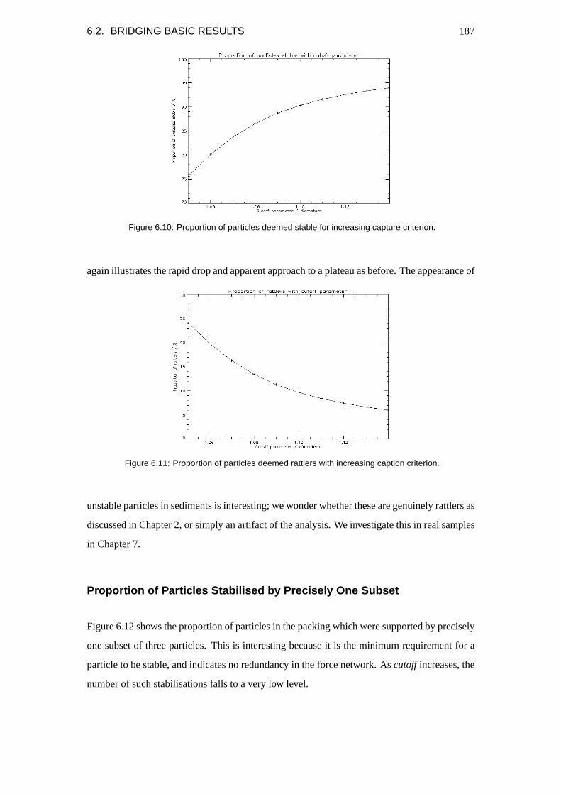
6.2. BRIDGING BASIC RESULTS 187
Figure 6.10: Proportion of particles deemed stable for increasing capture criterion.
again illustrates the rapid drop and apparent approach to a plateau as before. The appearance of
Figure 6.11: Proportion of particles deemed rattlers with increasing caption criterion.
unstable particles in sediments is interesting; we wonder whether these are genuinely rattlers as
discussed in Chapter 2, or simply an artifact of the analysis. We investigate this in real samples
in Chapter 7.
Proportion of Particles Stabilised by Precisely One Subset
Figure 6.12 shows the proportion of particles in the packing which were supported by precisely
one subset of three particles. This is interesting because it is the minimum requirement for a
particle to be stable, and indicates no redundancy in the force network. Ascutoff increases, the
number of such stabilisations falls to a very low level.

188 CHAPTER 6. BRIDGES
Figure 6.12: Proportion of particles deemed to be stabilised by precisely one stabilising subset, withincreasing capture criterion.
Mean number of Stabilisations per Stable Particle
Figures 6.13, 6.14, and 6.15 refer only to those particles which are deemed stable.
Figure 6.13 is the mean number of stabilising subsets per stable particle, withcutoff. Some-
what surprisingly, perhaps, this relation is apparently close to being linear. This would not be
expected from the previous curves, which were all obviously non-linear. It is not clear from
this plot alone what inference can be drawn, other than that the mean number of stabilisations
for a given stable particle is apparently not directly proportional to the number of neighbours
that particle has. Since the mean number of stabilisations is related to redundancy in the force
network, this suggests that the degree of redundancy does not relate straightforwardly to the
coordination number. It is perhaps surprising that the number of stabilisations is so high. This
is for a very dense sample, which is clearly very much overstabilised. Figure 6.14 shows the
mean number of particles which participate in a given stable particle’s stabilisation. Note that
since a stabilising particle may appear in more than one stabilising subset, this is not simply
three times the number of stabilising subsets. In fact, the relationship between the mean num-
ber of stabilising particles is, unlike the mean number of stabilising subsets, not nearly linear.
In fact, its variation withcutoff is more similar in shape to that of the coordination number,
which is at first glance reasonable. For this reason, the ratio of the mean number of stabilising
particles per stable particle to the mean number of stabilising subsets per stable particle was
plotted; it is shown in Figure 6.15. In this, there is a clear trend towards lower values as the
cutoff parameter is increased. From this, we observe that as the number of potentially stabil-
ising particles (i.e. the coordination number) increases, the ratio decreases. Since the ratio is

6.2. BRIDGING BASIC RESULTS 189
Figure 6.13: Mean number of stabilising subsets per stable particle with increasing capture criterion.
of the number of stabilising particles to stabilisations, we see that as the number of neighbours
increases, the number of stabilising subsets increases faster than the number of neighbours.
Figure 6.14: Mean number of stabilising particles per stable particle, with increasing capture criterion.
We note the interesting point that the number of stabilising particles and the number of stabil-
ising subsets are approximately equal for smallcutoff. This is surprising, and even more so
when we realise that the mean coordination number is also about the same at this point. As far
as we can tell, the number of stabilising subsets is simply coincidentally the same here. The
coincidence between the mean coordination number and the number of stabilising particles is
probably more interesting, and we discuss this further in light of the results for samples with a
range of volume fraction (Chapters 7 and 8).
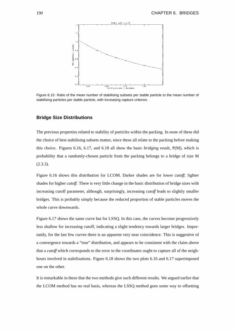
190 CHAPTER 6. BRIDGES
Figure 6.15: Ratio of the mean number of stabilising subsets per stable particle to the mean number ofstabilising particles per stable particle, with increasing capture criterion.
Bridge Size Distributions
The previous properties related to stability of particles within the packing. In none of these did
the choice of best stabilising subsets matter, since these all relate to the packing before making
this choice. Figures 6.16, 6.17, and 6.18 all show the basicbridging result, P(M), which is
probability that a randomly-chosen particle from the packing belongs to a bridge of size M
(2.3.3).
Figure 6.16 shows this distribution for LCOM. Darker shades are for lowercutoff; lighter
shades for highercutoff. There is very little change in the basic distribution of bridge sizes with
increasing cutoff parameter, although, surprisingly, increasingcutoff leads to slightly smaller
bridges. This is probably simply because the reduced proportion of stable particles moves the
whole curve downwards.
Figure 6.17 shows the same curve but for LSSQ. In this case, the curves become progressively
less shallow for increasing cutoff, indicating a slight tendency towards larger bridges. Impor-
tantly, for the last few curves there is an apparent very near coincidence. This is suggestive of
a convergence towards a “true” distribution, and appears to be consistent with the claim above
that acutoffwhich corresponds to the error in the coordinates ought to capture all of the neigh-
bours involved in stabilisations. Figure 6.18 shows the two plots 6.16 and 6.17 superimposed
one on the other.
It is remarkable in these that the two methods give such different results. We argued earlier that
the LCOM method has no real basis, whereas the LSSQ method goes some way to offsetting

6.2. BRIDGING BASIC RESULTS 191
Figure 6.16: Bridge distributions for increasing capture criterion using the LCOM method for decidingupon stabilisations.
Figure 6.17: Bridge distributions for increasing capture criterion using the LSSQ method for decidingupon stabilisations.
the problem of overcounting the neighbours due tocutoffbeing too large. As we shall see later,
the LSSQ results correspond closely to those from simulations of granular material. We take
these two remarks to imply that LSSQ is a much better choice, and we continue to use this in
preference to LCOM.
It is not clear whether there is any correspondance between the bridges found using these two
methods. It may be that they are essentially finding the same bridges, but that LCOM has a
greater tendency to chop them up where LSSQ retains their full size. If they give a different
set of spatial locations, then it casts severe doubt on the ability of bridges to describe load-
bearing structures. We do not do this here, but suggest that a means of investigating correlations
between the spatial positions of the bridges would give an interesting measure of the usefulness

192 CHAPTER 6. BRIDGES
Figure 6.18: Bridge distributions for increasing capture criterion: comparison between LCOM and LSSQmethods for deciding upon stabilisations.
of the bridging analysis.
Mean and Maximum Bridge Size
Figure 6.19 shows the mean bridge size withcutoff for both LSSQ (top, black) and LCOM
(bottom, red). In each case, this is only weakly dependent on the capture criterion. Whilst
in the LSSQ case, the trend is upwards as one might expect, in the LCOM it is very slightly
downwards. The downward trend in LCOM is probably due to the reduced number of stable
particles, as argued above, and is not informative. Figure 6.20 shows the maximum bridge size
Figure 6.19: Mean bridge size with increasing capture criterion for LSSQ (top, black) and LCOM (bottom,red).
with cutoff, again for LSSQ and LCOM. The trend for LCOM is much as for the mean bridge

6.2. BRIDGING BASIC RESULTS 193
size. For LSSQ, the sudden sharp increase followed by a plateau may show that there is a lower
limit on cutoffabove which the essentially the same bridges are found. If so, it agrees with the
argument above.
Figure 6.20: Maximum bridge size with increasing capture criterion for LSSQ (top, black) and LCOM(bottom, red).

194 CHAPTER 6. BRIDGES

Chapter 7
Stability and Bridging Results for
Pegrav∼1
7.1 Introduction
This Chapter describes the results of a large number of experiments on samples of the PMMA
particles known as ASM246 in purecis-decalin, over a wide range of volume fractions. These
particles have gravitational Peclet number∼1, and therefore sediment rapidly under gravity,
but are not yet granular. We first consider some general properties of these packings. We
then consider what we call stability properties, which are a step in complexity lower than full
bridging. We then consider the basic bridging properties in this system. It is important to
realise in this chapter that when we consider stability and bridging properties, this isnotmeant
to imply that the packing under consideration is genuinely stable or bridged in any mechanical
sense. It is simply important to know how these analyses behave even in samples which are
certainly not stable under gravity.
7.2 Description of the Samples Used
The gravitational Peclet number for the samples used in this section was found using 2.4.1
Pegrav =mBgh
kBT=
43π∆ρr3 gh
kBT=
43π∆ρg
1kBT
r4.
Given thatρPMMA = 1.188gcm−3, ρdec = 0.897gcm−3, r = 1.09 × 10⁻⁶, andT = 295K,
this givesPegrav = 4.15 ∼ 1 for the samples used in this section.
195

196 CHAPTER 7. STABILITY AND BRIDGING RESULTS FOR PEGRAV∼1
Sample Nominal Φ
1 0.40
2 0.42
3 0.44
4 0.46
5 0.48
6 0.50
7 0.52
8 0.54
Sample Nominal Φ
9 0.56
10 0.57
11 0.58
12 0.59
13 0.60
14 0.62
15 0.64
Table 7.1: Initial volume fractions of samples prepared.
Samples prepared
Samples were prepared according to the description in Chapter 5 to have nominal volume
fractions in the rangeΦ = 0.40-0.64 (Table 7.1). A large stock solution was created in each
case at the desired concentration by dilution from the previous concentration, to reduce the
relative weighing errors and ensure that the systematic errors were the same between samples.
Samples this dense cause handling problems. They are so viscous that they cannot realistically
be transferred from the stock solution to the sample cell by syringe or pipette in a reasonable
experimental time. Furthermore, the work of Haw [159] shows that particles of this size cannot
be reliably syringed at volume fractions greater than aroundΦ'55% due to “jamming”, or
“self-filtration”, at the entrance to the constriction. For this reason, sample cell 2 (§5.3.3) was
used. This allowed the use of a spatula to “scoop” the denser samples into the sample cell. This
was considered a fairly unreliable operation, but was unavoidable, and we bear this in mind.
As the stock solution was diluted, it became, as expected, a good deal more “runny”. There
was a noticeably sharp change in the sample at aroundΦ ' 0.60, slightly higher than one
might expect compared with the glass transitionΦ ' 0.58. Shortly after this point, it was no
longer reasonable to use a spatula, so a Pasteur pipette was used. This has a large diameter and
the pipetting was carried out as slowly and in as controlled a manner as possible (although a
Pasteur pipette is inherently badly suited for precision operations). There are clearly significant
uncertainties imposed by this procedure. We deal with these later and thereby show that the
results are still convincing.

7.3. BASIC SAMPLE PROPERTIES 197
Stack Time / sec
1 0
2 100
3 200
4 300
5 400
6 500
7 602
8 702
Stack Time / sec
9 802
10 902
11 1002
12 1203
13 1403
14 1604
15 1804
16 2004
Stack Time / sec
17 2505
18 3005
19 3505
20 4509
21 5514
22 6518
23 7522
24 8527
Stack Time / sec
25 9531
26 10535
27 11539
28 12544
29 13548
30 14553
31 15567
Table 7.2: The times at which stacks were captured during long time series. Times vary slightly betweenexperiments, up to around ±3 seconds at the higher times, but much lower for earlier stacks.
Imaging of the samples
A region of size' 40µm× 40µm× 20µm and whose central lateral plane was20µm into the
bulk of the sample in each case. Shortly after preparation, six different regions were chosen at
random lateral positions from each sample and a single stack captured from each. Following
this, a single region was imaged for the next approximately four hours. Five further stacks were
taken at further random lateral positions after the experiment had finished.
Since all of the samples sediment rapidly, these experiments give a large number of samples
over a large range of volume fractions.
7.3 Basic Sample Properties
Before investigating the stability and bridging properties of these variousPegrav ∼ 1 samples,
we consider some basic properties of the packings. These allow us to assess how nearly hard-
sphere-like the particles are, as well as providing a clearer picture of the evolution of the sample
as sedimentation occurs. In particular, we consider the evolution of the measured volume
fraction, the mean coordination number and the radial distribution function.

198 CHAPTER 7. STABILITY AND BRIDGING RESULTS FOR PEGRAV∼1
7.3.1 Comparison of nominal volume fraction with actual volume frac-
tion
The volume fraction that will be used from now onwards is the number calculated using the
method described in Section 5.2.4 (subsection “A local volume fraction”), using a particle
diameter of2.18µm. It is useful to know how this compares with the “nominal”, or target,
volume fraction that the system was supposed to have. This is as described in Section 5.2.4.
Figure 7.1 shows the relationship between these two numbers. The ordinate is the intended
volume fraction.
Figure 7.1: Relationship between the nominal (i.e. intended) volume fraction and the actual volumefraction as measured by the mean Voronoı volume per particle.
Also shown in this Figure as a dashed line is the expected case where the nominal volume
fraction is the same as the one calculated using the Voronoı technique, and a least-squares
best fit to the data (solid line). The relationship between the two is reasonably reassuring; the
agreement is quite good. We argued earlier 5.2.5 that the sample preparation volume fractions
should be correct relative to one another, that is, the dominant errors should be systematic. It
does not appear that there were significant systematic errors. The errors are certainly larger
for the lowerΦ samples, but this is reasonably justifiable. In preparing the samples, it was
inevitable that there was a small delay between sealing the sample cells in the laboratory and
transferring them to the microscope stage. This delay was somewhere in the region of ten to
fifteen minutes. As we shall see shortly (Figure 7.6), the sample can sediment significantly
even in this time, and this can explain why some of the samples were significantly more dense
than expected (and also why others were not). More care should have been taken to ensure that
the time involved in the transfer of the sample to the microscope stage was controlled, thereby

7.3. BASIC SAMPLE PROPERTIES 199
ensuring that the experiment was carried out on a sample of the desired volume fraction and
not some other value. Since the volume fraction is taken from the data, however, this does not
prejudice our analysis.
The other extreme of volume fraction appears to be slightly lower than expected. The very
highest volume fractions were always in doubt due to the difficulty of manipulating samples
this viscous. The last few (highestΦ) samples were scooped from a very viscous sample by
spatula; it was noted at the time that this was an unsatisfactory arrangement. It is therefore not
surprising that these do not achieve the expected volume fraction.
Each point in this Figure is the mean of the volume fractions of six stacks captured at the be-
ginning of the experiment. The error bars shown are one standard deviation of the distribution
of these values in each case.
7.3.2 Radial distribution functions
Figure 7.2 shows the radial distribution function for each of the samples studied. There is one
g(r) for each sample, and they are arranged according to a “rainbow” colour code which we
will use from now on. The initially sparse samples (low sample numbers) are at the red end,
while increasingly dense samples are progressively towards the blue.
Figure 7.2: Pair correlation functions for all decalin samples with nominal volume fractions 0.40 to 0.64
(see Table 7.1), shortly after preparation. The palette is a rainbow one; initially more dense samples aremore blue. The full g(r) is shown on the left, while the right-hand image shows the first peak expanded.
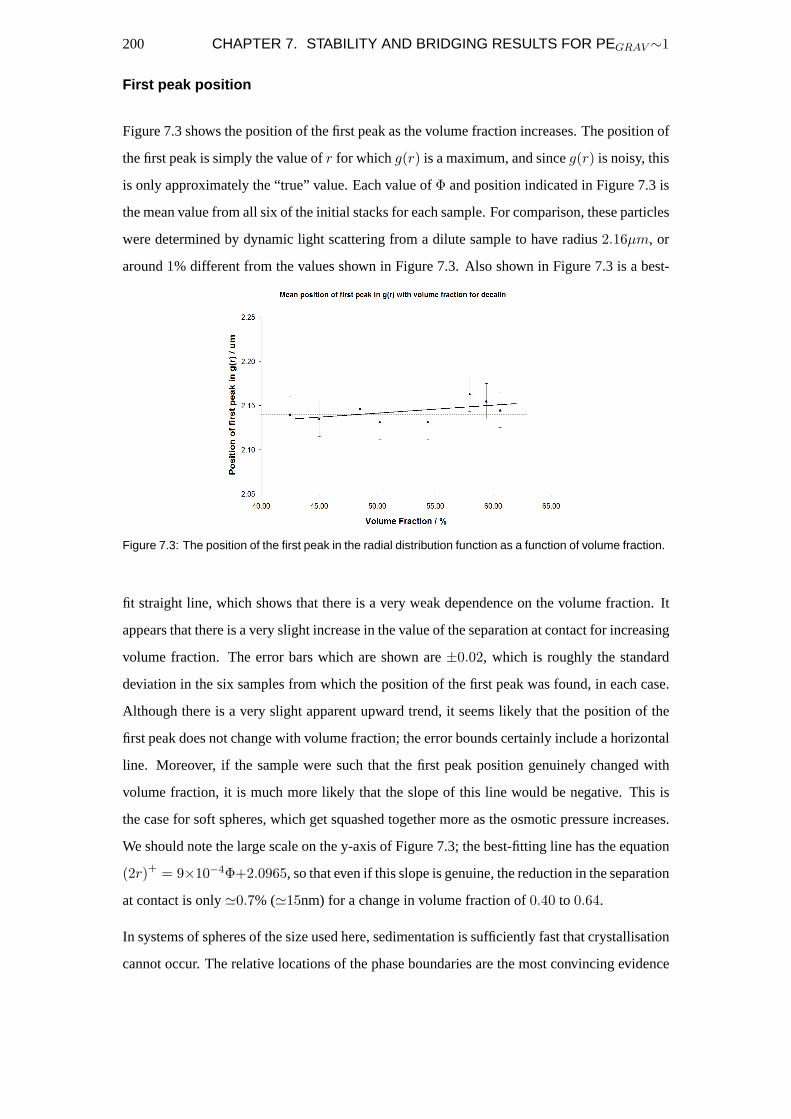
200 CHAPTER 7. STABILITY AND BRIDGING RESULTS FOR PEGRAV∼1
First peak position
Figure 7.3 shows the position of the first peak as the volume fraction increases. The position of
the first peak is simply the value ofr for whichg(r) is a maximum, and sinceg(r) is noisy, this
is only approximately the “true” value. Each value ofΦ and position indicated in Figure 7.3 is
the mean value from all six of the initial stacks for each sample. For comparison, these particles
were determined by dynamic light scattering from a dilute sample to have radius2.16µm, or
around1% different from the values shown in Figure 7.3. Also shown in Figure 7.3 is a best-
Figure 7.3: The position of the first peak in the radial distribution function as a function of volume fraction.
fit straight line, which shows that there is a very weak dependence on the volume fraction. It
appears that there is a very slight increase in the value of the separation at contact for increasing
volume fraction. The error bars which are shown are±0.02, which is roughly the standard
deviation in the six samples from which the position of the first peak was found, in each case.
Although there is a very slight apparent upward trend, it seems likely that the position of the
first peak does not change with volume fraction; the error bounds certainly include a horizontal
line. Moreover, if the sample were such that the first peak position genuinely changed with
volume fraction, it is much more likely that the slope of this line would be negative. This is
the case for soft spheres, which get squashed together more as the osmotic pressure increases.
We should note the large scale on the y-axis of Figure 7.3; the best-fitting line has the equation
(2r)+ = 9×10⁻⁴Φ+2.0965, so that even if this slope is genuine, the reduction in the separation
at contact is only'0.7% ('15nm) for a change in volume fraction of0.40 to 0.64.
In systems of spheres of the size used here, sedimentation is sufficiently fast that crystallisation
cannot occur. The relative locations of the phase boundaries are the most convincing evidence

7.3. BASIC SAMPLE PROPERTIES 201
of hard-sphere-like behaviour (see Section 2.2.3), but in the absence of this information, and
as argued in 2.2.3, the position of the first peak is a good alternative. In sparse systems of
spheres with soft interaction potentials, a particle’s nearest neighbours are pushed away. As
the osmotic pressure increases (Figure 2.5) with volume fraction, the nearest neighbour shell
is forced closer to the central particle. Figure 7.3 provides evidence that the particles here are
behaving adequately as hard spheres.
7.3.3 Relationship between Mean Coordination Number and Φ
The mean coordination number has been used in this enquiry sometimes since it can be mea-
sured without knowing the particle radius accurately in advance. It is the mean number of
neighbours that a particle has, where a neighbour is a particle that lies within a specified dis-
tance of the current particle. If the particle radius is not known accurately, one can use the mean
coordination number at a given absolute distance. This can be converted to a relative distance
once the radius is known. The radial distribution function is “well-behaved” for the samples
studied here insofar as that whether the neighbour capture criterion is, say,1.05 diameters or
1.10 diameters does not change the qualitative behaviour. It is useful, however, to know the
relationship between the two.
Figure 7.4 shows the relationship between the measured coordination number at1.1 diameters
and the volume fraction. Each point on this chart is derived from a single stack. There were
15 experiments, each at a different nominal initial volume fraction. Each experiment is shown
in a different colour, using the same colour scheme as in Figure 7.2. Figure 7.4 (left) shows
all of the data together, and illustrates that there is a fairly tightly-defined relationship between
the two quantities. Figure 7.4 (right) shows the same data, but with points from successive
experiments (that is, initial volume fractions) displaced in the y-direction. These show that the
relationship between mean coordination number and volume fractionwithin a given sampleis
closer still, and that the differences between experiments increase the spread. This is probably
due to differences in image quality between the experiments. Although the data shown in
Figure 7.4 show a reasonably tight relationship between volume fraction and mean coordination
number for all of the samples, there are slight apparent systematic differences. Samples starting
with low volume fraction, for exampleΦ ' 0.40 sediment toΦ = 0.64, with a coordination
number of' 8, whereas those samples which start at volume fractionΦ ' 0.60 finish at the
same volume fractionΦ = 0.64, but with coordination number' 7.5. This is apparently a

202 CHAPTER 7. STABILITY AND BRIDGING RESULTS FOR PEGRAV∼1
systematically difference. It is impossible to tell whether this is real effect or simply due to the
difference in image discussed above. However, if it is true, then it suggests that some degree of
history, perhaps evening some degree of jamming, is important in the sample preparation. We
cannot say any more than this here.
Figure 7.4: Relationship between coordination number and volume fraction. Colours are as for Figure7.2.
It is sometimes useful to convert between the two values. Figure 7.5 shows a cubic fit to these
data,Φ = a+bx+cx2+dx3, with x the mean coordination number. There is no justification for
this fit other than that it appears to model the data reasonably well over the range studied. There
are vastly more points than there are adjustable parameters (630 versus four), so interpolation
using this fit seems justifiable. The parameters of this fit area=0.0015, b=0.0851, c=0.0064,
andd=− 0.0009.
Figure 7.5: A cubic polynomial fit to allow approximate conversion between mean coordination numberat 1.1 diameters and the volume fraction.
7.3.4 Sample Evolution
None of the samples was prepared in an initially stable state; even the most dense samples had
to settle under gravity. The simple packing properties of volume fraction and mean coordina-
tion number were followed in time.

7.3. BASIC SAMPLE PROPERTIES 203
Volume fraction
Figure 7.6 shows the evolution of the volume fraction for each sample, with the colour scheme
as before. There are31 points for each sample, one corresponding to each of the stacks taken
during the time series. These points are for only one stack each time, so are relatively noisy.
It seems from these, however, that there is a limiting volume fraction which is achieved fairly
quickly (within around four hours), and that the rate of change of the volume fraction is pro-
portional to the difference between the current volume fractionΦ(t) and the limiting volume
fraction.
Figure 7.6: Evolution of volume fraction with time, for each sample.
If we accept the apparently obvious conclusion that there is a long-time limiting volume frac-
tion, ΦMRJ1, then at first glance we would suggest an evolution according to
dΦ(t)dt
= α(ΦMRJ−Φ(t)),
whereα is a arbitrary proportionality constant. This equation can be solved straightforwardly,
given the initial conditionΦ(t=0)≡Φi, to give
Φ(t) = ΦMRJ−(ΦMRJ−Φi) exp{−αt}.
Figure 7.7 (left) shows a best-fit to the relationy = a−b exp{−ct} for the sample which was
initially at Φ=0.425 (nominally 0.42), witha=0.617, b=0.183, andc=2.9×10⁻⁴. The fit is
not particularly convincing, but the shape is sufficiently close to suggest that the basic idea is
sound.1We presumptiously assume this is the Maximally Random Jammed state.

204 CHAPTER 7. STABILITY AND BRIDGING RESULTS FOR PEGRAV∼1
Figure 7.7: Fits to volume fraction with time. A simple model provides a reasonable fit (left), but anadjustment, whilst unjustified, makes a convincing fit (right).
Figure 7.7 (right) shows the result of minor adjustments to this model. By raising the power
exponential by an unknown parameter, that is, by fittingy = a−b exp{−ctd}, we achieve a
much more convincing shape. Here,a=0.646, b=0.236, c=0.005, andd=0.644, which means
thatΦMRJ = 0.646 andΦMRJ − Φi=0.236. Both of these numbers compare well with the
expectationΦMRJ ' 0.64 andΦMRJ−Φi ' 0.640−0.425=0.215. The additional power,d,
corresponds to a differential equation governing the evolution ofΦ of
dΦ(t)dt
= αd(ΦMRJ−Φ(t))× td,
so although the fit is good, it is not easy to justify. It is not obvious why the time should be
scaled by some factor∼ 23 .
Consider sedimenting particles as they cross an arbitrary lateral plane in the sample. The flux
across such a surface is proportional to the sedimentation velocity. It seems plausible that the
rate of densification (that is,dΦdt ) is proportional to the flux of particles across this surface.
Thus dΦdt ∝ Vsed to a first approximation. It is well known that the sedimentation velocity of
a particle in a dense suspension is a non-obvious function of volume fraction, see for example
[100]. It is therefore no real surprise that the simplistic model described above does not capture
perfectly the behaviour of the system. The above noted dependence ont23 presumably happens
to represent the non-linearΦ dependence for these samples. These data are good enough to be
analysed further, but this is left as a future exercise here. In particular, the above suggests that
the sample history is important in determining the evolution; it looks from Figure 7.6 as though
there may be a master curve onto to which the curves would all fall if the correct dependence
were found.
7.3. BASIC SAMPLE PROPERTIES 205
Lastly from this Figure we see that since each data point derives from a single stack, there
is a fair degree of noise on these plots. From the oscillations shown on these curves, we can
estimate a random error in the volume fraction from these stacks as± ' 0.01. This is of course
no substitute for a proper error treatment, but is reasonable. As usual, no systematic error can
be established from the data.
An important discussion of the apparent size of the particles
We make a brief aside to discuss an important anomaly that arose in the analysis of these
results. As we saw in the last section, the position of the first peak in g(r) was at2r ' 2.14µm.
However, in order to produce Figures 7.1 and 7.6, a diameter of2r = 2.18µm was required
to produce the expected final volume fraction ofΦ'0.64. We have argued strongly before
that the correct radius to use in determining the volume fraction is the (half) the position of
the first peak maximum in g(r) (rather than some other value from e.g. light scattering). This
contradiction must be explained. We chose to use the value ofr which gave the expected value
for the volume fraction of the sediment, namelyΦ ' 0.64. In fact, the volume fraction ought
really to have been calculated using the value (at most)2r = 2.14µm, giving a final volume
fraction for the sediment of around60-61%. We have chosen to take the view that it is more
likely that the first peak of g(r) is for some reason found to be lower than its true value, as it
seems more likely that the sediment is really achieving the (some would argue) volume fraction
corresponding to random close packing. Also, as we shall see in the next chapter, results from
the density-matched samples seem to back up this particular figure. The question remains
why the first peak should be so much ('2%) too low. One possibility is that non-core-shell
particles, even with the modifications I have made (via SSF refinement) will tend to be deemed
too close to one another in the densest packings. This is a suitable explanation to explain this
observation. The other possibility is simply that the packings are genuinely not achieving the
highest densities.
As we shall see in the next chapter, density-matched samples were made up according to the
same protocol. In these, the same range of nominal volume fractions was prepared. The
maximum and minimum volume fractions obtained in practice were extremely close to those
obtained in the decalin only case,if the larger figure for the radius is used. This supports the
use of2r = 2.18µm. This is an unresolvable situation, and we continue assuming that the
radius of the particles is larger than g(r) would suggest.

206 CHAPTER 7. STABILITY AND BRIDGING RESULTS FOR PEGRAV∼1
Mean coordination number
Over the same experiment, the mean coordination number evolved, as one would expect given
Figure 7.4, in a similar fashion to that shown in Figure 7.8. In much the same way as for the
Figure 7.8: Evolution of coordination number with time.
volume fraction, there appears to be a limiting value for the mean coordination number, which
is achieved after around four hours. Figure 7.6 suggests an estimate of the error in the mean
coordination number of±0.2. As in the volume fraction evolution, there are slight systematic
differences between the curves. The trend that we noted earlier is clearer here; the initial less
dense samples appear to show a slight tendency towards final states of higher coordination
number, suggesting a slight history dependence. The noise is however quite dramatic, and,
given variations such as that shown by the lowest (green) curve which clearly does not fit the
overall trend, it is not reasonable for us to argue any more.
Radial Distribution Function, g(r)
Figure 7.9 shows the evolution of the radial distribution function for one particular sample as
it sediments. One of the lower volume fraction samples was chosen, to illustrate this evolution
over a wide range of volume fractions. In this case, Sample 2 (Φi = 0.42) was used; this
sample is shown in orange in Figures 7.6 and 7.8. Firstly from this Figure, it is obvious how
significant an improvement the SSF refinement has been. Not only do the first peaks rise much
more sharply below the particle diameter, but all of the peaks are obviously much sharper and
taller.

7.3. BASIC SAMPLE PROPERTIES 207
Figure 7.9: Evolution of g(r) for a sample of initial volume fraction Φi = 0.42 as it sediments; “time” runsinto the page, later (denser) stacks are redder. This sample is the orange one in Figures 7.6 and 7.8.In both images, successive distributions are offset by 0.2 diameters in x and 0.25 in y for clarity. Theleft-hand image is for coordinates obtained using the centroid method only, while the right-hand one isfollowing SSF refinement. This provides a nice illustration of the success of the method in a randomly-chosen sample. Note that these g(r)s are noisy as they are for a single stack.
It is clear from both these distributions that as the volume fraction increases, the first peak
becomes taller, and the subsequent peaks and troughs become sharper and better defined. It
is also clear, much more obviously so in the post-refinement curves, that the shape of the
second peak in particular has evolved. Particularly noticeable (significantly, only in the post-
refinement curves) is the splitting of the second peak, which is characteristic of glasses. What
is perhaps most significant here, however, is that even over this wide range of volume fraction,
the changes ing(r) are quite small. The height of the first peak, arguably the most sensitive
function of volume fraction, changes from' 3.00-4.25 (c.f. ' 2.00-3.25 for the unrefined
coordinates). Theg(r) shows almost no change between the “glassy” samples numbers10-15
(the “reddest” six).
Figure 7.10: Evolution of g(r) for a sample of initial volume fraction Φi = 0.42. This Figure contains thesame information as Figure 7.9, but the slightly different format reveals different features.

208 CHAPTER 7. STABILITY AND BRIDGING RESULTS FOR PEGRAV∼1
Thatg(r) is not useful in distinguishing between packings is frustrating. Certainly, it should be
a useful quantity for comparing between light scattering and microscopy results. If the particle
coordinates were known to arbitrarily high precision and the sample perfect (σ = 0) then the
g(r) would show much higher first peaks (certainly greater than ten, and much narrower). This
is unavoidable when studying real colloidal systems.
As well as being of demonstrably limited usefulness for the samples studied here, we note that
g(r) does not contain all of the available information about general sphere packing, given the
sphere coordinates. It is clear thatg(r) contains no information on the angular distribution
of a particle’s neighbours, for example. Some studies have considered these properties (see
for example [19]. Furthermore, investigations by Mark Haw on two ostensibly similar sphere
packings of identical volume fraction and very similarg(r) have shown differences in their
“remoteness”, a measure which quantifies void in packings [170]. One of the sphere packings
was produced by him using a Monte-Carlo based technique, the other by myself using the
well-known event-driven Molecular Dynamics Lubachevsky-Stillinger algorithm. The most
likely interpretation of this is that although the packings are at the same volume fraction, they
are microstructurally different but not sufficiently so thatg(r) is noticeably affected. The
most straightforward example of this would be if the samples have differing (but still “small”)
degrees of crystallisation (the Lubachevsky-Stillinger algorithm in particular is known to allow
varying degrees of crystallisation depending on the input parameters). The inference from this
is thatg(r) is not especially sensitive to the sort of microstructural details that are of interest in
this enquiry.
We reiterate that althoughg(r) is a useful measure for comparison with light scattering results,
it does not make full use of the local information that confocal microscopy allows, and to a
certain extent the findings above are not surprising.
7.4 Stability Results
In this section, we discuss what we refer to asstability results. These are properties relating
solely to how each particle is stabilised by its neighbours in response to an applied force. We
do not yet discuss any mutual stabilisations or other bridge properties. The stability results
are obtained by running the bridge finding analysis up to the point where we must make the
decision of which stabilising subset is the “correct” one. This corresponds to running the

7.4. STABILITY RESULTS 209
Bridge Finder code up to Step 5 as defined in Table 6.1. We discuss these in some detail since
they do not rely on the most doubtful assumption of the bridging analysis but are nonetheless
interesting. We discuss the stability results over the full range of volume fraction, and present
the results both as a function of volume fraction and of mean coordination number at1.1
diameters. It is important to emphasise that to the best of our knowledge there are no theoretical
predictions for any of the quantities discussed in this section.
7.4.1 An interesting observation
In some samples of another latex, ASM151, sediments were observed to exhibit unexpected be-
haviour. On several occasions, when a sediment was observed over a period of twenty minutes
at intervals of one minute, a small sub-population of individual (that is, apparently not spatially
correlated in any way) particles were observed to “jiggle”, that is, move from side to side as
though caged by their neighbours. The remaining particles were apparently very nearly static,
for a period of at least ten hours. Furthermore, Figure 7.11, which shows a randomly-chosen
slice in the x-z direction from one of these samples, appears to show some sort of structural
anisotropy in the sample.
Figure 7.11: A representative slice in the x-z direction, which appears to show a preference for a particulardirection in the sample.
It is very important to remember that the eye, although extremely accomplished at picking
out patterns which are algorithmically very difficult to find, equally cannot be relied upon.
We hope that bridges may be related to these structures, and may therefore emerge from the
analysis described below.

210 CHAPTER 7. STABILITY AND BRIDGING RESULTS FOR PEGRAV∼1
7.4.2 Stability Properties
Proportion of particles deemed stable
Figure 7.12 shows the proportion of particles which are deemed stable for a range of volume
fractions. There is a clear trend in these data. We have no idea what to expect of this re-
lationship, except that the proportion of stable particles should be in the region0.95-1.00 at
a volume fraction ofΦ ' 0.64, since the expected number of unstable particles (“rattlers”,
if the particles are genuinely unstable in the packing) in a MRJ samples is up to around5%
(2.1.6,). Inevitably the proportion of particles deemed stable will fall for lower volume frac-
tions. Equally, for lower volume fractions, there will always be particles arranged, by chance,
so that the stability test finds them able to provide support. That is, there will always be a
certain proportion of particles deemed stable at all finite volume fractions. The relationship be-
tween the two quantities is until now unknown. Whilst it does seem reasonable that the number
of particles deemed stable should increase with coordination number and volume fraction, the
shape of this curve could not be predicted on intuitive grounds.
Figure 7.12: Proportion of particles deemed stable in samples of increasing packing density.
Importantly, the fact that the proportion of particles deemed stable is not volume fraction in-
dependent rules out its being simply an artefact of the analysis; it is apparently a real effect.
Furthermore, the analysis, even without resorting to looking to mutual stabilisations, has iden-
tified a sub-population of particles from the sample which cannot be determined from the typ-
ical measures used to quantify sphere packings, most notably the radial distribution function.
This is the first of a number of measures in this thesis which benefit from local information.
Furthermore, if the unstable particles really do correspond to rattlers, then we have extracted

7.4. STABILITY RESULTS 211
dynamical information (the rattlers move while the rest do not) from a single snapshot of the
system at that point. That is, we can infer dynamical information from a static image.
Figure 7.12 is encouraging in that the proportion of particles deemed stable at the expected
MRJ density ofΦ'0.64 is'0.95. That is, at about the density of the expected random close
packed state, the number of unstable particles corresponds with the permissible number in such
a state. The MRJ state, however, should ideally have no unstable particles (we argued earlier
that where these occur, they are a consequence of the protocol used to generate the packing,
rather than inherent in the MRJ packings). We now consider whether the particles which are
found to be unstable are genuinely rattlers, or whether they simply are the result of experimental
uncertainty.
Importantly, we note that there is no convincing plateau in this Figure which would allow
mechanically stable packings over a range of packing fractions (i.e. in the region random loose
packing to random close packing). If these packings somehow reproduced anything similar to
those of Onoda and Liniger ([91]), then there would be a flat or nearly flat region of this curve
from aroundΦ = 0.55 upwards, where the proportion of stable particles was around95% or
greater. If the stability properties calculated here genuinely reflect the stability of the packing,
then it is clear that the packings generated here are inherently different from, for example, those
of Onoda and Liniger.
A closer look at unstable particles
Figure 7.13 shows the proportion of unstable particles as a function of volume fraction. This is
simply 100 minus the previous value. To have confidence in the stability properties, we must
assess whether these “unstable” particles are genuinely rattlers as discussed in Chapter 2. We
anticipate that experimental uncertainty means that these two quantities are not identical, but
hope that they are related. This section discusses the relationship between them.
Figure 7.14 gives a representation of the unstable particles for four different volume frac-
tions. The top left image is the most important, since it shows the unstable particles in a
packing of volume fractionΦ'0.64 (actually it is a single sample of determined volume frac-
tion Φ=0.6422, or taking into account the errorΦ=0.64(1)). The remaining images are for
Φ=0.59(1), Φ=0.51(1), andΦ=0.45(1). In these images, it is clear that the number of unsta-
ble particles increases (the proportion of particles which are stable in these particular samples
are8.63%, 11.63%, 30.48%, and43.76% respectively.). In the last two, there are no obvious

212 CHAPTER 7. STABILITY AND BRIDGING RESULTS FOR PEGRAV∼1
Figure 7.13: Proportion of particles deemed to be unstable in samples of increasing packing density.
spatial correlations. In the first two, particularly the first, it seems as though there is a small
amount of “bunching” of the unstable particles. We look at this more closely by plotting his-
tograms of the particle coordinates for each of these images (and bear in mind the coordinate
system as defined in Figure 4.4).
Figure 7.15 (top) shows these histograms. Each row in this Figure corresponds to one sample,
the highest being at the top. The left, middle and right images in each case are the distribution
of x-, y-, and z-coordinates respectively, all in bins of size five pixels. (These results are quoted
in pixels, this is of no consequence here.)
Figure 7.15 shows that for the highest volume fractions, there is indeed a bias towards certain
spatial locations. In the histograms of the x-coordinates, there is a slight tendency towards one
side of the image. At the lower volume fractions, however, the distribution is convincingly
flat. A similar situation also occurs for the y-distribution, but much more pronounced. There
is a very strong bias towards the (upper and lower) edges of the images when there are very
few unstable particles. Again in this case, when the number of unstable particles increases
(lower volume fractions), the distributions become very nearly flat. We should emphasise at
this point that it is unlikely that this is due to edge effects in the data themselves, since we
took considerable precautions to avoid this. Firstly, all particle coordinates within a border of
width one particle radius around the images was disregarded, so that particle coordinates here
are reliable in this respect. Secondly, when determining whether particles could be stable, a
further border of width one radius was used outside of which stability was not tested (although
particle within this second border were used to test the stability of neighbouring particles which
were just within the second border).

7.4. STABILITY RESULTS 213
Figure 7.14: A representation of the spatial distribution of unstable particles for samples in the rangeΦ = 0.64 (top left) to 0.45 (bottom right). For more detail, see text and Figure 7.15.
The histograms of the z-coordinates are perhaps more illuminating. Again there is a similar
trend towards a more even distribution for less stable samples. Interestingly here, however,
there is a very obvious increase in unstable particles for a narrow range of low z-coordinate,
for all of the volume fractions. Even for the least stable samples, the pronounced peak at
very low z remains. Since the images were captured from deeper in the sample to shallower
(Secton 4.1.3), this means that there is a clear jump in the number of unstable particles at the
deepest portion of the sample. This is significant because the signal-to-noise ratio drops with
increasing depth into the sample. The most reasonable interpretation of this is that there is
at this point a sudden decrease in the reliability of the particle coordinates (as respects their
ability to determine stability). Certainly the obvious alternative, that there are genuinely more
unstable particles in this narrow range, seems extremely unlikely.
There are two strong statements which we can make in light of these results. The first is that
we have inadvertently discovered a means of (in principle) defining an objective measure of
image quality which permits the stability analysis. It is clear from the histograms that the
image quality becomes sufficiently bad only in the last bin, that is, the last five pixels. We infer
that image quality has fallen below an acceptable level only in these pixels, and could therefore

214 CHAPTER 7. STABILITY AND BRIDGING RESULTS FOR PEGRAV∼1
Figure 7.15: Spatial distribution of unstable particles for samples of volume fraction Φ = 0.64, 0.60, 0.51,and 0.45 (top to bottom). For each sample, the distribution of particle coordinates is shown in the x-, y-,and z-directions (left, middle, and right, respectively). The binsize is five pixels in each case.

7.4. STABILITY RESULTS 215
develop an objective criterion from this.
The second conclusion is that if we accept the first, then there must presumably be some in-
homogeneity in the imaging which has given rise to less reliable particle coordinates towards
the top and bottom, and to a lesser extent, the sides of the captured images. The distribution
of rattlers is not uniform in the lateral plane when it presumably is in the sample. Even if
there were genuinely some spatial dependence, we would expect that there was no difference
between either of the two directions (i.e. x- and y-) in the lateral plane, since these are de-
fined arbitrarily by the orientation of the sample on the microscope state. We conclude that
the imaging system, despite giving satisfactory (to the eye) images, was not producing images
of everywhere constant SNR. Surprisingly, the only obvious inadequacy of the VT-Eye is the
presence of vertical intensity bands of width∼10-100 pixels in the images. These could almost
explain the bias seen in the x-coordinate histograms, but this bias is small compared with the
vertical bias (to which no obvious image imperfection corresponds).
The above arguments strongly suggest that at least some of the unstable particles are not true
rattlers. Although we cannot provide solid evidence, we suggest that limitations in the particle
coordinates result in a certain “baseline” or background proportion of unstable particles in
any packing. The fact that the distributions are more nearly flat for greater “rattler” numbers
suggests that there is a genuine population of unstable particles in any packing as well as those
background rattlers. As the number of genuine unstable particles increases, these outweigh
the background which becomes negligible. This means that the points in Figures 7.12 and
7.13 could be systematically higher (Figure 7.12) or lower (Figure 7.13) by up to around five
percent, and does not settle the issue of whether there are any true rattlers in these packings.
None of this, however, detracts from the clear trend in the proportion of particles deemed stable
with coordination number, which would be altered only systematically.
7.4.3 Stabilisation properties for stable particles
Having established how the proportion of stable particles varies with packing density, and
that the stability criterion seems genuinely to reflect the number of stable particles, we now
consider some properties relating to the manner in which a known stable particle is stabilised.
Specifically, we have argued that each stable particle can be stabilised by a number of separate
sphere triplets. Here we consider how the number of stabilisations per stable particle depends
on the mean coordination number and volume fraction.

216 CHAPTER 7. STABILITY AND BRIDGING RESULTS FOR PEGRAV∼1
Stabilising particles per stable particle
Figure 7.16 shows how the mean number ofparticleswhich provide stabilisation to a known
stable particle varies with volume fraction. This is fairly intuitive measure of how well sta-
bilised a given stable particle is. This Figure shows a clear trend towards a greater number of
Figure 7.16: Mean number of stabilising particles per stable particle for samples of increasing packingdensity.
particles involved in a given stable particle’s stabilisation for increasing coordination number.
The relation is reasonably close to being linear, which is interesting. More significantly, over
the range of densities studied here, the number of stabilising particles per stable particle is very
similar to the mean coordination number for all particles in the sample. This tends to suggest
that for a stable particle,all of its neighboursare involved in its stabilisation. This is perhaps
surprising at first glance, but is believable. The first natural intuitive objection is that some of
the neighbouring particles lie above (that is, have a higher centre of mass than) the stable par-
ticle. It is important to realise that a particle can belong to another particle’s stabilising subset
even if its centre of mass lies above that of the stable one. This takes a moment’s thought, but
is actually fairly obvious. The exception is when one particle liesdirectly above the other, in
which case the lower cannot be stabilised by the higher. For more details on exactly what is
required for a particle to be confined (caged) by its neighbours, please refer to [93].
The important observation from this Section is that apparently all of a particles contacting
neighbours are involved in its stabilisation. This is certainly not obvious in advance, and is
interesting.
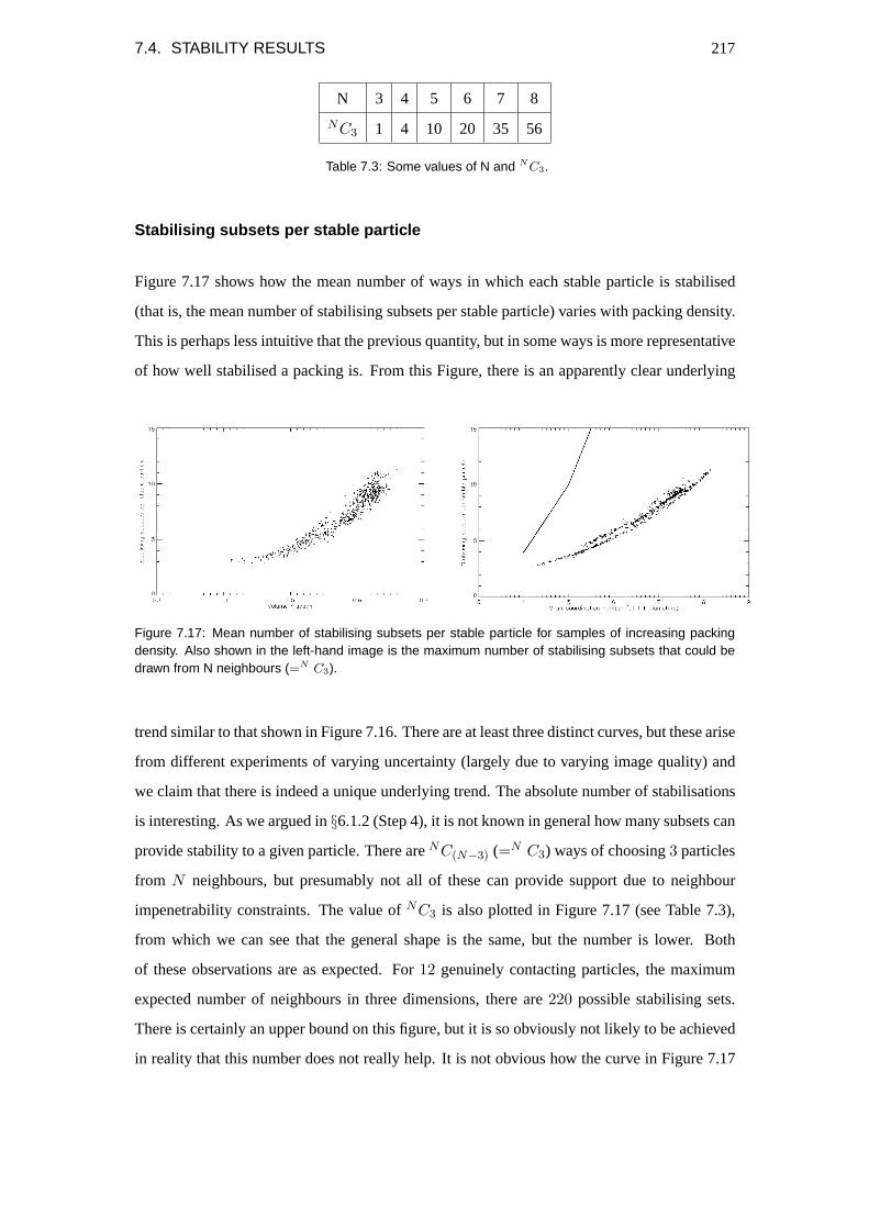
7.4. STABILITY RESULTS 217
N 3 4 5 6 7 8
NC3 1 4 10 20 35 56
Table 7.3: Some values of N and NC3.
Stabilising subsets per stable particle
Figure 7.17 shows how the mean number of ways in which each stable particle is stabilised
(that is, the mean number of stabilising subsets per stable particle) varies with packing density.
This is perhaps less intuitive that the previous quantity, but in some ways is more representative
of how well stabilised a packing is. From this Figure, there is an apparently clear underlying
Figure 7.17: Mean number of stabilising subsets per stable particle for samples of increasing packingdensity. Also shown in the left-hand image is the maximum number of stabilising subsets that could bedrawn from N neighbours (=N C3).
trend similar to that shown in Figure 7.16. There are at least three distinct curves, but these arise
from different experiments of varying uncertainty (largely due to varying image quality) and
we claim that there is indeed a unique underlying trend. The absolute number of stabilisations
is interesting. As we argued in§6.1.2 (Step 4), it is not known in general how many subsets can
provide stability to a given particle. There areNC(N−3) (=N C3) ways of choosing3 particles
from N neighbours, but presumably not all of these can provide support due to neighbour
impenetrability constraints. The value ofNC3 is also plotted in Figure 7.17 (see Table 7.3),
from which we can see that the general shape is the same, but the number is lower. Both
of these observations are as expected. For12 genuinely contacting particles, the maximum
expected number of neighbours in three dimensions, there are220 possible stabilising sets.
There is certainly an upper bound on this figure, but it is so obviously not likely to be achieved
in reality that this number does not really help. It is not obvious how the curve in Figure 7.17

218 CHAPTER 7. STABILITY AND BRIDGING RESULTS FOR PEGRAV∼1
would look for higher volume fractions. Although we would like to know this, it is difficult to
achieve volume fractions greater than this.
It is hard to interpret exactly what this curve means. Intuitively, the number of stabilising
subsets per stable particle is a measure of redundancy. Only one subset is necessary to provide
support, but it does seem reasonable that increasing the number of stabilisations increases the
probability that the particle will be stabilised in practice. We have not made any assessment of
the tenability of the stabilisations, nor taken into account that in general, the stabilising particles
are themselves free to move under an applied load. Bearing these in mind, the most reasonable
conclusion is that this quantity is simply a particular set of geometrical properties that describes
the packing, and its variation with volume fraction and mean coordination number is simply a
useful but not profound quantitative measure.
Figure 7.18 shows how the ratio of the number of stabilising particles to the number of stabil-
ising subsets varies with packing density. This is a measure of how overstabilised the packing
is, and how important individual particles are. The number of subsets alone measure over-
stabilisation, but the ratio contains information about how many stabilisations each particle is
responsible for. It therefore says something about the important of individual particles, but we
are not able to think of any deeper meaning for this quantity.
Figure 7.18: Ratio of mean number of stabilising particles to mean number of stabilising subsets perstable particle.
Stable particles stabilised by precisely one subset
Figure 7.19 shows the proportion of stable particles which are stabilised by one single subset.
Once again, while there is no prediction for this quantity, there is a clear trend. It is surprisingly

7.4. STABILITY RESULTS 219
small: note that even atΦ'0.40, where less than half of the particles are stabilised, only around
15% of stable particles are stabilised by a single subset. This is quite a surprising result; most
stable particles are stabilised in more than one way. The physical meaning of this quantity is
Figure 7.19: Proportion of particles deemed to be stabilised be precisely one subset in samples ofincreasing packing density.
not easy to establish intuitively. All we can really say is that as we approach the highest packing
densities, the stable particles in the packings (which by this stage is virtually all of them) are
essentially all stabilised in more than one way. This is a statement that there is a high level of
redundancy in the force-bearing network that supports the packing.
It is worth discussing what we had expected this quantity to show. The minimum requirement
for a sediment of hard spheres to be stable is presumably that each particle is stabilised by one
subset only. Since sediments have been observed for packings in a region loosely termed ran-
dom loose packed to random close packed, it is reasonable to suggest that the loosest possible
stable sediment, random loose packing, corresponds to the situation in which every particle is
stabilised by one and only one subset. While reasonable, this picture is clearly not relevant
here. The first reason is that in these samples, there is not a sufficient plateau in stable particles
(Figure 7.12) to volume fractions lower than around the requiredΦ'0.55. More importantly,
it is clear that the proportion of stable particles stabilised by only one subset never gets near
to one for any realistic volume fraction. We must remember that the number of stabilisations
will tend to be overcounted due to the excess of neighbours (recall that a particle’s neighbours
are all those within a certain cutoff, which is larger than the diameter). Even taking this into
account, it seems unlikely that the proportion of stable particles stabilised by only one subset
will coincide with a volume fraction corresponding to random loose packing.

220 CHAPTER 7. STABILITY AND BRIDGING RESULTS FOR PEGRAV∼1
7.5 Bridge Results
Having studied the stability properties and found them to show clear and fascinating trends, and
have well-defined values even in evidently not stable packings, we now examine the bridging
properties of these same packings.
7.5.1 Bridge Size Distributions
Figure 7.20 (left) shows the distribution of bridge sizes generated using the LSSQ criterion, for
a cutoff value of1.1 diameters. All of the results for the samples discussed above (and detailed
in Table 7.1) are shown in this Figure; the black is the most dense (nominallyΦ = 0.64),
with an obvious trend from light blue to red (for nominalΦ = 0.40) for decreasing density.
Although it seems that the shape of all of the curves is broadly similar, it is clear that there is
a much smaller probability of finding a randomly-chosen particle to belong to a bridge of any
size for samples of lower density. The right-hand image in this Figure shows the same result,
but this time with a sample distribution from a simulation of granular materials superimposed
in green. The granular result is easily identified; it is the highest curve. It is reasonably obvious
Figure 7.20: Bridge size distribution for samples of increasing packing density (samples as given in Table7.1). The lowest density samples are shown in red (beginning with nominal Φ = 0.40), and as the volumefraction increases to Φ = 0.64, the curves move upwards (and change from red to blue to light blue. Thelast curve is black, and has nominal Φ = 0.64. The right-hand image shows the same data, but this timewith a result from the granular case superimposed in green. This is the highest curve.
from this that these are not quite the correct distributions to plot. The reason that lower volume
fractions have lower probabilities for a randomly-chosen particle to belong to a bridge is simply
that fewer of the particles are stable and therefore could not belong to a bridge (Figure 7.12).

7.5. BRIDGE RESULTS 221
Rather, we see that the more sensible thing to do is to plot the probability that a randomly-
chosen known-stable particle belongs to a bridge of size M.
These distributions are obtained by dividing the above distributions by the proportion of parti-
cles in these packings which were deemed stable. The result of this is shown in Figure 7.21.
In this case, it is clear that there is a much closer coincidence between the curves. They very
Figure 7.21: Bridge size distribution for samples of increasing packing density, this time normalised tothe number of stable particles.
nearly lie one on top of the other, with a slight trend towards smaller bridges for less dense
samples, which is not surprising. In particular, there is now a convincing comparison between
the granular case and the more dense colloidal ones.
Figure 7.22 (left) shows how the mean bridge sizeM (of bridges withM>1) varies with
volume fraction. There is no reason to suppose that this relationship should be linear, but,
despite a fairly large spread in the data, this is surprisingly close to being true. As the bridge
size distributions above show, the dependence, although clear, is a weak one. The right-hand
image here shows the variation of the same quantity with coordination number.
Figure 7.23 (left) shows the dependence of the maximum bridge sizeMmax on the volume frac-
tion. Though there is a slight increase in (mean) maximum bridge size with increasing volume
fraction, there is no useful rule relating the two. Interestingly, it seems that the spread of max-
imum bridge size increases with volume fraction. This is probably reflective of the tendency
of experimental uncertainty, which will presumably result in incorrect mutual stabilisations, to
“chop up” larger bridges. There is no justification for this remark beyond intuition; we main-
tain that the effect of uncertainty will be more often to reduce a bridge’s size artificially than
to increase it. This is a hunch that ought to be investigated further, and most easily realisable

222 CHAPTER 7. STABILITY AND BRIDGING RESULTS FOR PEGRAV∼1
Figure 7.22: Mean bridge size for samples of increasing packing density.
using simulation data for known “bridged” samples and introducing random perturbations to
the particle coordinates to mimic experimental uncertainties.
Figure 7.23: Maximum bridge size for samples of increasing packing density.
7.6 Testing for Bridges in Other Directions
Throughout this enquiry we have concentrated on bridges as structures which are stable against
gravity. It has always been implicit that these are somehow formed by gravity. It is not clear
however that gravity should impose a structure on the sample; it could equally well exploit
structures which are present in these packings, that is, gravity need not cause any structural
changes to all the packing to be capable of supporting its own weight.
In this Section, we consider the possibility that a particular packing is capable of supporting a
load applied in a different direction to that of gravity.

7.6. TESTING FOR BRIDGES IN OTHER DIRECTIONS 223
A cubic region from a sample of densityΦ'0.64 (simply a “fully sedimented” sediment) was
processed to find bridges as described above. Thesameraw data were then rotated electroni-
cally through90 degrees (by applying a standard rotation algorithm), and these new coordinates
run through exactly the same bridge finding procedure. The angle chosen was arbitrary. Figure
7.24 shows the result of this analysis.
Figure 7.24: The effect of rotation on the distribution of bridge sizes. These two are remarkably similar;the distribution of bridge sizes is not affected by rotation by π
2, nor is it likely to be for any arbitrary
rotation.
It is clear from this Figure that the bridge size distribution is identical following this operation.
The insets to this Figure illustrate that the effect of this operation is to test the packing for
bridges capable of supporting a load in another direction. The upper right is an illustration of
an applied load in the “standard” (downwards) direction, whilst the lower left is an illustration
that the effective applied force now acts perpendicular to gravity.
The bridges are identical for a completely different applied force. If one believes that bridging
describes the ability of a packing to support an applied force, then it is clear that the packing
is equally well able to bear a load in another direction, and presumably this applies in any
direction. This is equivalent to saying that supposing we were able to perform the rather un-
usual experiment of turning off gravity briefly, then turning it on in a direction perpendicular
to the laboratory “up” direction, then supposing the laboratory were off sufficiently remarkable
design, the sample would not respond; it is already stable against this applied force.
224 CHAPTER 7. STABILITY AND BRIDGING RESULTS FOR PEGRAV∼1
This is a very significant observation. It is in agreement with Kegel’s assertion that even if
gravity is responsible for the glass transition ([74]), then its effect is not related to an irreversible
structure being imposed on the sample by gravity. This allows two possibilities, the first that
gravity imposes some special structure which does not permit crystallisation, but which relaxes,
beginning immediately the gravitational field is “switched off” (centrifugation is ceased, in
their case). The second is that gravity merely takes advantage of inherent structures within the
packing. The latter is more simple, and therefore naturally preferable, but is also intuitively
correct. We can do better than this, provided we believe in the bridging analysis; if we do, then
it is clear that the sample studied contains structures which equally well able to support a load
in at least two different directions, and presumably any. Importantly, this means that unlike real
macroscopic granular materials, colloidal sediments are not fragile as defined by Cates [9].
We are not aware of any simulations having tested for bridges in other directions. This is a test
which should be performed by them without delay.

Chapter 8
Stability and Bridging Results for
Pegrav∼10−3
8.1 Introduction
This Chapter describes the results of an identical set of experiments to that described in the
previous Chapter, but this time with a mixture ofcis-decalin and CHB to very nearly match
the density of the solvent with that of the particles. The resultant gravitational Peclet number
would be zero if the density matching procedure were perfect. Of course it is not, but it is
sufficiently good that the particles take at least several days to form a sediment at1000g, sug-
gesting gravitational Peclet number ofPegrav∼10−3. For ease of comparison, in this Chapter
we always present the results alongside those from the previous Chapter.
8.2 Description of the Samples Used
Samples Prepared
Essentially the same set of experiments were performed. The exact volume fractions differed
slightly; they are shown in Table 8.1. As these were performed in exactly the same manner as
in the previous Chapter, no further comment is necessary. The samples were imaged in exactly
the same way as forPegrav∼1, and at the same times (Table 7.2).
225

226 CHAPTER 8. STABILITY AND BRIDGING RESULTS FOR PEGRAV∼10−3
Sample Nominal Φ
1 0.40
2 0.42
3 0.44
4 0.46
5 0.48
6 0.50
7 0.52
8 0.54
9 0.56
10 0.57
11 0.61
Table 8.1: Initial volume fractions of density-matched samples prepared.
8.3 Basic Sample Properties
As in the previous Chapter, we consider some basic sample properties.
8.3.1 Comparison of nominal volume fraction with actual volume frac-
tion
Figure 8.1 shows the relationship between the target volume fraction and the actual volume
found from the data, both as described before.
There are several clear features in this graph. The first is that the uncertainties are much smaller
than they were in the decalin-only case. This is almost certainly because the image quality was
much higher and therefore the particle coordinates are better. This is seen in the sharper radial
distribution functions in Section 4.7.5. The second obvious feature is that the slope of the
“expected” curve very closely matches the observed one. This is encouraging, and in particular
is consistent with the earlier argument that lower volume fraction samples sediment before they
can be measured. The discrepancies this causes are not present here. Lastly, the calculated
volume fraction is systematically higher (by slightly less than one percent) than the target one.
This is consistent with, and indeed much smaller than the maximum of, the earlier argued error
in the stock solution.

8.3. BASIC SAMPLE PROPERTIES 227
Figure 8.1: Relationship between the nominal (i.e. intended) volume fraction and the actual volumefraction as measured by the mean Voronoı volume per particle for the density-matched samples.
8.3.2 Phase Diagram
Figure 8.2 shows a pseudo-phase diagram, in which a fully crystalline sample is indicated
by the value “2”, a partially crystalline sample by “1”, and a value “0” denotes no observed
crystallisation. This appears to suggest a coexistence region ofΦ'0.42-0.54. This is consistent
Figure 8.2: A phase diagram for the density-matched particles which illustrates that the phase boundarywas difficult to discern. A value of 2 indicates that the sample crystallised, whereas a value of 1 indicatesthe sample partially crystallised and probably belonged to the coexistence region.
with the particles carrying a slight charge. Although it is tempting to identify the lack of
crystallisation atΦ'0.58 with the glass transition, we remember that density-matched samples
are claimed to crystallise [74]. We should note that this phase diagram represents the state of

228 CHAPTER 8. STABILITY AND BRIDGING RESULTS FOR PEGRAV∼10−3
the system after the experiment, which was a maximum of around15 hours. It may be that
crystallisation occurs after this.
8.3.3 Radial distribution functions
Figure 8.4 shows the radial distribution function for each of the samples studied, shortly after
they were prepared. Figure 8.3 shows the colour code used to distinguish between these sam-
ples. Note the reverse order; higher volume fractions are plotted with lower (bluer) colours.
Φ = 0.61 Φ = 0.40
Figure 8.3: The colour code used to distinguish between density-matched samples. As indicated, thehigh volume fraction samples are “bluest”.
Figure 8.4: The radial distribution functions for density-matched samples with volume fraction in the range'0.40-0.60, as indicated in Table 8.1. Denser samples (the “more blue” ones), have first peaks which arehigher and occur at lower separations.
The radial distribution function is quite different from that in the previous Chapter. The evo-
lution from low to high density is much more in keeping with what we would expect from
simulations of hard spheres, insofar as the first peak height increases dramatically. This re-
flects the higher accuracy of the particle coordinates for the density-matched samples; the peak
height increased only slightly in the decalin samples because they were “washed” out to a
greater extent by the inaccuracies.
We must note here that though we have claimed that the particles are charged in this system,
the rdfs are much sharper. We said earlier that this was due to the differing refractive index
mismatches in the two systems, so we cannot reliably compare them. However, it seems likely

8.3. BASIC SAMPLE PROPERTIES 229
that charged systems should have if anything less sharp rdfs, and therefore the fact that they are
in fact sharper tends to suggest that these particle coordinates are known to higher accuracy.
Of course, g(r) could legitimately be different due to the effects charge and or the change in
Pegrav; it is impossible to tell from these data. Figure 4.24, which compared the rdfs obtained
for the sample decalin-only system for a poor quality image and a good quality image go some
way to answering this; the very high quality image of the decalin-only sample gives rise to a
very sharp g(r). This makes a convincing case that where g(r) is not sharp, it is because of the
inaccuracy of finding particle coordinates rather than a reflection of genuine properties of the
sample.
An important feature of this Figure is that there is a marked change in the position of the first
peak. It is clear that as the volume fraction is increased, the peak moves to shorter distances.
We examine this in more detail.
First peak position
Figure 8.5 shows the position of the first peak as the volume fraction is changed. Unlike in the
decalin-only case, it is clear here that the position of the first peak is changing with volume
fraction. This is strongly suggestive of softness in the interaction potential. The error bars are
once±0.02, which is representative of the spread of the data from several different samples. As
Figure 8.5: The position of the first peak in the radial distribution function as a function of volume fraction.
well as being consistent with the suggestion of a charge on the particles by the phase diagram,
this suggestion is strongly backed up by the shape of Figure 8.5. At the highest densities,

230 CHAPTER 8. STABILITY AND BRIDGING RESULTS FOR PEGRAV∼10−3
where the osmotic pressure is very high (Figure 2.5), the particles are forced ultimately into
contact, giving a first peak position of around the value of2.18 µm argued in the previous
Chapter. As the density is reduced, the osmotic pressure falls rapidly, so the particles are able
to force themselves apart. It appears that there is sudden change in the shape of the curve in
Figure 8.5 atΦ ' 0.54. This would be understandable in a system where the interactions
were hard sphere-like, since this is about the point where crystallites are first observed (and
would therefore be consistent with the variation in osmotic pressure). This does not explain
this observation, but does support the particles being charged. The dashed line is horizontal,
and is simply to indicate the region of over which the relationship is nearly flat.
8.3.4 Relationship between Mean Coordination Number and Φ
Figure 8.6 shows the relationship between the volume fraction and mean coordination number
for the density-matched samples. As in the decalin-only case, there is a well-defined relation-
Figure 8.6: The relationship between coordination number and measured volume fraction for the density-matched samples. The left-hand image shows all of the samples, with each one shown in a differentcolour. For samples of volume fraction Φ'0.45-0.55 there is evidence of crystallisation. The right-handimage shows results from only stacks captured shortly after preparation.
ship between the volume fraction and the mean coordination number. That is, mean coordina-
tion number is a good measure of the system density. Figure 8.6 (left) shows all of the data
from the density-matched samples, including some which have crystallised. It is reasonably
clear which these are; the less tightly defined clusters are ones in which samples of the same
coordination number have a range of volume fractions (and they all occur in the [initial] vol-
ume fraction rangeΦ'0.46-0.54). Figure 8.6 (right) shows only the supercooled samples, that
is, the datasets collected at the beginning of the experiment.

8.3. BASIC SAMPLE PROPERTIES 231
The most important feature of this relationship is that it is quite different from the decalin
case. At the highest densities, the mean coordination number is around eight (as it was in the
decalin case, Figure 7.4). Very importantly, however, at the lowest volume fractions (Φ'0.40),
the mean coordination number for the density-matched samples is around2, whereas it was
around4.5 in the decalin case.
We rely on this difference shortly. We must note that this means that the systems are not
behaving in the same manner. It also implies that at least one of the systems is not behaving
as a hard sphere system. Given the evidence so far that the first peak does not change position
with Φ for the decalin samples whereas they do for the density-matched ones, we argue that
Figure 7.4 shows theΦ-coordination number relationship for a hard sphere system, and that
Figure 8.6 shows this relationship for a different (softer) pair potential. We argued in Section
8.3.2 that the particles were charged. This seems to be consistent with the above result; at
lower densities the particles tend not to have as many neighbours as they are able to avoid one
another, whilst at higher densities they simply cannot achieve this.
8.3.5 Sample Evolution
Since the samples prepared here were density-matched, the time evolution ought to be quite
different from the samples used in the previous Chapter.
Volume Fraction
Figure 8.7 shows how the volume fraction evolves in time for the density-matched samples.
This Figure is reassuring; the samples do not change their density over the course of the exper-
iment. They cannot be sedimenting, so the density-matching procedure appears to have been
successful. In this case, we see that the error in the volume fraction, as inferred from the scatter
in this dataset, is around±0.005 for the denser samples. Interestingly, the error is apparently
larger (±'0.01) for less dense samples. This makes sense, since these are based on fewer
particles, although it was not clear in Figure 7.6, presumably because of the rapid change in
Φ. We assume that this increased error holds there too. It is conceivable that the fluctuations
in volume fraction could be real here, rather than just statistical, but we could not distinguish
between these possibilities from these data.

232 CHAPTER 8. STABILITY AND BRIDGING RESULTS FOR PEGRAV∼10−3
Figure 8.7: The evolution of the sample volume fraction (in time) for density-matched samples at a rangeof initial densities. Note the important point that there is no change over the course of the experiment.
Mean coordination number
Figure 8.8 shows how the mean coordination number evolves in time for the density-matched
samples. The mean coordination number is once again apparently subject to much less noise
Figure 8.8: The evolution of the mean coordination number in time for density-matched samples at arange of initial densities. Once again, these do not change over the course of the experiment.
thanΦ. It is obvious from the Figure that the sample has not sedimented appreciably during
the experiment.

8.3. BASIC SAMPLE PROPERTIES 233
Radial Distribution Function, g(r)
Figures 8.9 to 8.12 show the evolution of g(r) over the course of the experiments for a selection
of volume fractions. We have established that the volume fraction does not change over the
course of the experiments, so these do not evolve in the same way as those for the decalin
samples. These rdfs do however give some indication of where crystallisation is occurring.
Figure 8.9: The evolution of g(r) for a density-matched sample of initial volume fraction Φi = 0.45.
Figure 8.9 shows the evolution of g(r) for a sample of volume fractionΦ=0.45. According to
the phase diagram above, which was based on visual inspection of the samples, there was a
small amount of crystallisation in this sample. This is not evident in the evolution of g(r). This
is not worrying however, it suggests that the amount of crystallisation was simply too small to
show up in g(r). Moreover, the volumes imaged may just happen to have been of fluid regions,
which is very likely if the degree of crystallisation is small.
Figure 8.10: The evolution of g(r) for a density-matched sample of initial volume fraction Φi = 0.51.
Figure 8.10 shows the evolution of g(r) for a sample of volume fractionΦ=0.51. There is
clearly some crystal in the regions used to calculate this distribution, although here too it seems
as though there must still have been a predominance of fluid in the imaged volumes.
Figure 8.11 shows the evolution of g(r) for a sample of volume fractionΦ=0.54. In this case,
there is clearly a lot of crystal in the imaged volume. This evolution of the degree of crystal is

234 CHAPTER 8. STABILITY AND BRIDGING RESULTS FOR PEGRAV∼10−3
as expected as the coexistence region is crossed.
Figure 8.11: The evolution of g(r) for a density-matched sample of initial volume fraction Φi = 0.54.
Figure 8.11 shows the evolution of g(r) for a sample of volume fractionΦ=0.59. In this case,
there increasing degree of crystallinity with increasing volume fraction has clearly been re-
versed; there is very little if any evidence of crystallisation (there is a slight sharpening of the
second peak, which suggests a small increase in order.)
Figure 8.12: The evolution of g(r) for a density-matched sample of initial volume fraction Φi = 0.59.
It is clear from the above Figures that we have captured the process of crystallisation occurring.
We did not set out to do this, so the sampling rate is not probably not ideal; it would be possible
however to study some properties of the crystallisation process from these date. We did not
attempt this here.

8.4. STABILITY RESULTS 235
8.4 Stability Results
8.4.1 Stability Properties
Proportion of particles deemed stable
Figure 8.13 shows the proportion of particles which are stable in the density-matched case,
along with the results for the decalin samples (and are as plotted in Chapter 7). In this and
the rest of the plots in this Section, the black curves are the results for the density-matched
samples, while the red are those for the decalin case.
Figure 8.13: The proportion of particles deemed stable in samples of increasing packing density withvolume fraction (left) and coordinate number (right) for both the density-matched (black curve) and non-density-matched (red curve) samples.
Figure 8.14 shows the proportion of particles which are not stable. These two Figures set
Figure 8.14: The proportion of particles deemed unstable in samples of increasing packing densitywith volume fraction (left) and coordinate number (right) for both the density-matched and non-density-matched samples.
the tone for the rest of the stability results. Firstly, the density-matched results show a trend
with increasing volume fraction (left) which is similar to that for the decalin case, but which

236 CHAPTER 8. STABILITY AND BRIDGING RESULTS FOR PEGRAV∼10−3
apparently reveals more features. There is once again a tightly-defined (more so in this case)
relationship between the proportion of stable particles and the volume fraction. Moreover, the
behaviour for high volume fraction is as expected ('97% of particles stable). They show a drop
with decreasing packing fraction, as expected, but also show a another apparent near-plateau
at lower (but still high) volume fractions. This overall sigmoidal shape is entirely unexpected,
and indeed the lower portion in particular is surprising. Note that these data are for all samples,
crystalline included, so it does not relate to the any phase transition (the crystalline samples
can be seen as small excursions in several places), despite the proximity of the lower turning
point to the argued melting point. It is clear from this curve that reducing the volume fraction
in this region has little effect on the proportion of the particles in the packing which are stable.
To understand how this can be so, refer to Figure 8.6, in which a similar flattening appears.
This is the first intimation of an important point that carries throughout the rest of this thesis.
For the purpose of stability determination, it is mean coordination number rather than volume
fraction which counts.
This realisation is beautifully illustrated by Figure 8.13 (right), where we show the variation
of the proportion of stable particles with the mean coordination number. This Figure is re-
markable, and the agreement between the two datasets is striking. No error bars are shown;
the errors are taken to be implied by the spread of the data. By this reckoning, the agreement
is perfect. It is abundantly clear that the proportion of stable particles in a random packing of
spheres follows a well-defined curve as a function of mean coordination number. We justify
calling these systems random since the density-matched samples must presumably comprise
randomly-distributed particles. There is at least no reason to suppose otherwise. If this is
true, then the agreement between the two systems suggests that the decalin-only system is also
random.
Note that discerning this difference is only possible because of the inadvertent difference be-
tween the two systems; if they had both behaved perfectly as hard spheres, we would have not
have noticed this important distinction.
At this point, it seems as though the volume fraction is no longer a useful parameter. It turns
out that this is indeed the case. It is perhaps not surprising that this is so, since the methods
used in this thesis are extremely dependent on interparticle contacts.

8.4. STABILITY RESULTS 237
8.4.2 Stabilisation properties for stable particles
Once again, we investigate further the stability properties for particles which are stable.
Stabilising particles per stable particle
Figure 8.15 shows how the mean number of particles which provide stabilisation to each stable
particle varies with density.
Figure 8.15: The number of stabilising particles per stable particle in samples of increasing packingdensity with volume fraction (left) and coordinate number (right) for both the density-matched and non-density-matched samples.
Here too there is a clear trend in both datasets, and it would be difficult to argue that these are
different. The number of particles involved in stabilising a known stable particle is therefore
simply a function of the coordination number in random sphere packings.
Figure 8.15 reveals, however, that this relationship is not well described by a single linear
relationship over the range of coordination number studied. The density-matched results have
therefore contributed additional information. In Section 7.4.3, we argued that the curve for the
decalin samples was nearly linear, and that over this range of volume fraction had a slope'1.
This implied that typically all of a particle’s neighbours were involved in its stabilisation.
The departure from the line with slope'1 is easily understood. The ordinate is the mean
coordination number for all particles in the sample, and not for the stable particles. This may
seem a little perverse, but we should remember that this is because the mean coordination has
been used primarily as an indicator of system density. We know from Chapter 6 that a stable
particle must have at least three neighbours. Since the mean coordination number at the lower
densities studied here is'2, it is obvious that those stable particles have a higher coordination

238 CHAPTER 8. STABILITY AND BRIDGING RESULTS FOR PEGRAV∼10−3
number. This does not allow the curve to have a slope of1 across the whole density range. We
should ultimately plot this curve as a function of coordination number for stable particles. One
thing we note is the point at which the curve apparently deviates from the line of slope one,
which is at around a mean coordination number of'4.5.
Note that increased noise at lower volume fractions is probably not significant. In these sam-
ples, there are many fewer particles; it is likely that this explains for the additional noise.
Stabilising subsets per stable particle
Figure 8.16 shows how the mean number of subsets which provide stabilisation to each stable
particle varies with density. Once again, these two curves are remarkably similar, and reveal
Figure 8.16: The number of stabilising subsets per stable particle in samples of increasing packingdensity with volume fraction (left) and coordinate number (right) for both the density-matched and non-density-matched samples.
that this quantity is simply a property of sphere packings of this coordination number. We
do note that both in Figure 8.15 and this to a greater extent in Figure 8.16 as well as the
overall trend there are several curves which very nearly fall onto the apparent trend, but not
quite. These only occur in the decalin-only (red) curves, which sediment during the experiment.
These separate curves belong to a few samples, and presumably arise from slight (systematic)
differences in the imaging conditions. The most likely possibility for this is a difference in the
image quality (perhaps the imaging parameters were not quite right, or the confocal aperture
position slightly wrongly). We do not doubt that these curves belong to the same overall trend.
Figure 8.17 shows the ratio of the mean number of stabilising subsets to the mean number of
stabilising particles with density. In this Figure, the curves clearly deviate at lower volume
fractions. This arises from the low volume fraction deviation in Figure 8.16, which we believe

8.4. STABILITY RESULTS 239
Figure 8.17: The ratio of the number of stabilising subsets per stable particle to the number of stabilisingparticles in samples of increasing packing density with volume fraction (left) and coordinate number(right) for both the density-matched and non-density-matched samples.
not to be significant. It seems probable that the ratio relationship is the same in both datasets.
As discussed in the previous Chapter, it is not clear exactly what this means, but it is further
evidence that the two systems are behaving in the same way with respect to their stability
properties.
Stable particles stabilised by precisely one subset
Figure 8.18 shows how the number of particles which are stabilised by precisely one subset
varies with density. In this Figure, the density-matched results reveal substantial new informa-
Figure 8.18: The proportion of stable particles which were stabilised by precisely one subset in samplesof increasing packing density with volume fraction (left) and coordinate number (right) for both the density-matched and non-density-matched samples.
tion. The behaviour demonstrated in the decalin case, Figure 7.19, is evident here. The lower
mean coordination number of the lower density samples in the density-matched reveals that
this distribution has a remarkably sharp turning point, and therefore qualitatively very different

240 CHAPTER 8. STABILITY AND BRIDGING RESULTS FOR PEGRAV∼10−3
behaviour below a certain critical mean coordination number.
The behaviour of the upper branch was discussed in Chaper 7 (alongside Figure 7.19), and is
reasonably understandable. As the number of neighbours in the sample decreases, the number
of ways a stable particle is stabilised drops. One might have assumed that the proportion
of stable particles stabilised by one subset decreased monotonically with decreasing packing
density. Figure 8.18 reveals that this is definitely not the case for the density-matched samples.
Whether this is also true for the decalin case is a very interesting question, and data from this
region would be useful. We have no explanation for this effect, but it is so pronounced that it
is an intriguing property.
The behaviour of the lower branch is peculiar. It says that as the density of the packing is
reduced, the proportion of stable particles which are stabilised by only one subset reduces
quickly. In other words, at low volume fractions, those relatively few particles which are stable
are stabilised in more than one way. This is a very strange result, and needs to be investigated
further.
Lastly for this property, we note that the turning point is at a mean coordination number of
around4.5.
8.5 Bridge Results
Figure 8.19 shows both the bridge distributions for the density-matched case (left) and the
decalin only case (right, duplicate of Figure 7.21).
8.5.1 Bridge Size Distributions
Figure 8.19 shows the bridge size distributions for the density-matched results (left), and
decalin-only results (right). Unlike in the decalin-only case, in which the bridge size distri-
butions were all very similar and belonged to a clear family, the distributions in the density-
profiles are quite different from one another. Starting from the lowest density samples, there
is a clear trend towards larger bridges. As the density increases, the bridge size distribution
tends towards the general shape familiar from the decalin case. Closer inspection of Figure
8.19 (left) reveals that actually the three or four most dense samples samples lie more-or-less
on top of one another, and are very similar to those in the right-hand image.

8.5. BRIDGE RESULTS 241
Figure 8.19: A comparison of the bridge size distribution for both the density-matched results (left), anddecalin-only results (right).
This seems odd, given the similarity of the stability properties. However, that we argued above
that the volume fraction was not the important property. If we consider instead the bridge
size distribution evolution as a function of mean coordination number, we realise that Figure
8.19 (left) encompasses a wider range, and it is no longer self-evident that the distributions are
qualitatively different. Figure 8.20 (left) makes this more explicit.
Figure 8.20: A comparison of the decalin-only bridges (left) and the density-matched bridges (right), thistime indicating the point at which the bridge size distribution departs from the apparent family of curvesevident for samples of higher mean coordination number.
In this Figure, two particular curves are highlighted. These are the least dense sample which

242 CHAPTER 8. STABILITY AND BRIDGING RESULTS FOR PEGRAV∼10−3
appearsjuststill to belong to the family, which has a mean coordination number of5.5, and the
most dense sample which clearly does not belong to this family and has a mean coordination
number of4.5.
We have no explanation for this sudden dramatic change in the bridging behaviour. A par-
ticularly fascinating question is it is common to both systems and therefore solely a property
of random sphere packings. We cannot know this because of the same lack of data discussed
above, and it be enlightening to have these data. It is worth emphasising how surprising this
result is; the bridge size distribution is apparently very robust at higher packing fractions, show-
ing only a very weak dependence on the sample density. Its significant qualitative change in
behaviour at this critical mean coordination number of'5 is unexpected, and if it were also
observed in the decalin-only system, would be a significant finding.
Figure 8.21 shows the mean bridge size with increasing sample density. This bridging property,
Figure 8.21: The mean bridge size with increasing sample density with volume fraction (left) and coordi-nate number (right) for both the density-matched and non-density-matched samples.
unlike any of the stability properties, does show a slightly different trend between the two sys-
tems. They are nonetheless quite similar. Moreover, the bridges in the decalin case are slightly
smaller. We suggest that this may be due to the inferior quality of the particle tracking in this
system. Since poorly-located particles will presumably tend to result in missed genuine mutual
stabilisations in preference to incorrectly identified not genuinely present mutual stabilisations
(that is, poor particle coordinations presumably reduce the size of a bridge more often than
increase it), then it is consistent that poorer quality data will apparently consist of fewer large
bridges.
Even if the trends are genuinely different, however, they are very similar compared with the
spread in the data.

8.5. BRIDGE RESULTS 243
Figure 8.22 shows the maximum bridge size with increasing sample density. In this case, as in
Figure 8.22: The maximum bridge size with increasing sample density with volume fraction (left) andcoordinate number (right) for both the density-matched and non-density-matched samples.
Figure 7.23, the spread of the data is so great that it is difficult to make any useful comment
based on it. It is certainly not possible to distinguish between the two systems using this
measure.
A Comparison with Granular Matter
Now that we have the bridge size distribution for both of the systems, we make an important
comparison. The bridging analysis is borrowed from simulations of granular materials, and it
is natural to compare the results obtained there with our own.
The granular materials simulations have not investigated stability properties, so no comparison
of these can be made. We should also reiterate that in these simulations there is essentially no
experimental uncertainty; their coordinates are known to machine precision, which is typically
∼10−8 (at worst,∼10−15 for double-precision variable types). Additionally, since their pack-
ings were generated electronically [87], they know which stabilisation arrested each particle
initially. There is therefore no difficulty in choosing the best stabilising subset. (Although
we make an important observation; they do not consider in this that a subsequently deposited
particle can fall into a position around a stable one such that it, in conjuction with two other
particles, then becomes capable of supporting the particlewhich is already stable. It is there-
fore perfectly possible for a computer-generated packing, even where the generating algorithm
does not permit the initial stabilisation to be by more than one subset, to generated such that
this is the case.)
A sample granular dataset was kindly provided by Gary Barker, and the corresponding bridge

244 CHAPTER 8. STABILITY AND BRIDGING RESULTS FOR PEGRAV∼10−3
distribution is shown on Figure 8.20. The agreement is compelling. (Note that the apparently
anomalously high points for large bridges arise from the small size of this dataset; my data also
show this behaviour if not sufficiently averaged.)
The samples in this enquiry, regardless of the gravitational Peclet number therefore show very
similar bridging behaviour, provided the mean coordination number is sufficiently high, both
to themselves and to simulated granular datasets.
We state this last point again to emphasise its importance: if we believe, as those who simulate
granular matter do, that bridges genuinely describe the ability of a packing to bear a load, then
a strong conclusion from this study is that packings of the same are equally well able to bear a
load regardless of whether they actually do. An important statement is therefore that gravity (or
any other unaxial load of similar magnitude) does nothing to induce load-bearing structures in
the packing. Where a load takes advantage of such structures, it is merely exploiting inherent
structures within the packing. This is a strong and significant conclusion.
8.6 A Discussion of Stability and Bridging in Both Systems
In Chapters 7 and 8 we have established a range of fascinating stability and bridging properties.
These appear to be purely geometric, and apply equally to Brownian and granular systems.
The quantities we have studied all show clear trends, but we have no predictions for what these
should have looked like; it is therefore difficult to comment on what they mean. In particu-
lar, the stability properties, which are properties of coordination number, behave in surprising
ways. What we have discussed is seemingly reasonable, although ideally we would be able to
compare it with other results. There are few studies into properties which could be related to
these quantities, but in this Section we outline some ideas.
Since the stability and bridging properties are designed to describe the effects of applied forces
on the packing, we might expect them to apply to a range of systems. The granular results are
encouragingly close to ours, and if the bridging results are useful in simulations of these, as
some authors claim, then our results suggest that they are equally useful in colloidal systems.
Stable granular systems only exist for a narrow range of densities, and we can now arguably go
further than this.
We have stability and bridging results for much lower densities than this; the decalin results are
for densities of down to around40%. The density-matched case give results which may be in-

8.6. A DISCUSSION OF STABILITY AND BRIDGING IN BOTH SYSTEMS 245
dicative of what occurs in hard sphere systems of lower densities than this. Rather than use the
stability analysis to try to explain bridging in mechanically stable packings such as sediments
and granular heaps, we can now investigate whether these quantities have any relevance to the
behaviour of non-mechanically stable stressed colloids. In particular, we recall the experiments
of Haw [159], in which jamming and “self-filtration” effects were seen for suspensions of large
particles above a certain critical volume fraction. The question is whether we can predict the
onset of jamming using the stability properties.
Isaet al. have begun to expand upon these experiments[171]. They force dense suspensions
of roughly2µm particles into confining geometries ('700µm) using relatively high pressures
('50-70 torr), and observe the resulting velocity profiles. They first observe jamming, as
described by Haw, atΦ'0.53. From Figure 8.13, we see that nothing particularly special
occurs here (for conversion between coordination number and volume fraction, see Figure 7.4;
importantly, we assume that this is the hard sphere relationship) in the stability properties.
About70% of particles are stable at this volume fraction. We should remember, however, that
the stability properties concern the ability of an individual particle to be supported against an
applied load, which concerns jamming on scales'5µm, whereas jamming (at least as studied
by Haw and Isa) is a very large scale ('700µm) phenomenon. Jamming of the sort Haw has
reported requires cooperative load-bearing structures, which was exactly the point of bridges.
Interestingly, the bridge size distribution shows a significant change for a mean coordination
number of'4.5-5 (Figure 8.20), which corresponds to a volume fraction of around45-48%,
which is sufficiently close to be worthy of further investigation.
Perhaps more interesting are the experiments of Lootens and co-workers [172]. Although
they relate to shear experiments, they are nonetheless similar, and we expect our work to be
relevant. They shear particles of various diameters in the range400nm to2.5µm in a Couette
geometry of gap size250µm. They observe jamming at much lower volume fractionΦ'0.42,
and at much lower applied stress (maximum'1 torr). This may reflect the narrower gap in the
system compared with that of Isa, or, more likely, a greater sensitivity of the latter technique.
The former experiments are after all rather crude. Notably, the stress required to jam the system
drops100-fold for an increase of volume fraction ofΦ=0.42 to Φ=0.48, see Figure 8.23. Very
importantly, the particle size has no effect on the jamming threshold. This strongly implies
that the jamming transition is a purely geometric one. Moreover, the shape of the jamming
transition line, which says that higher pressures are required to jam samples of lower volume
fraction are consistent with Figure 8.13; the proportion of stable particles in the packing does
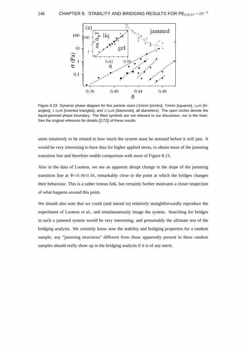
246 CHAPTER 8. STABILITY AND BRIDGING RESULTS FOR PEGRAV∼10−3
Figure 8.23: Dynamic phase diagram for five particle sizes (400nm [circles], 700nm [squares], 1µm [tri-angles], 1.5µm [inverted triangles], and 2.5µm [diamonds], all diameters). The open circles denote theliquid-jammed phase boundary. The filled symbols are not relevant to our discussion, nor is the inset.See the original reference for details ([172]) of these results.
seem intuitively to be related to how much the system must be stressed before it will jam. It
would be very interesting to have data for higher applied stress, to obtain more of the jamming
transition line and therefore enable comparison with more of Figure 8.13.
Also in the data of Lootens, we see an apparent abrupt change in the slope of the jamming
transition line atΦ'0.46-0.48, remarkably close to the point at which the bridges changes
their behaviour. This is a rather tenous link, but certainly further motivates a closer inspection
of what happens around this point.
We should also note that we could (and intend to) relatively straightforwardly reproduce the
experiment of Lootenset al., and simulataneously image the system. Searching for bridges
in such a jammed system would be very interesting, and presumably the ultimate test of the
bridging analysis. We certainly know now the stability and bridging properties for a random
sample; any “jamming structures” different from those apparently present in these random
samples should really show up in the bridging analysis if it is of any merit.

Chapter 9
Future Work
The work presented in this thesis has produced two distinct sets of results. The first is an
improvment to the widely available particle location routines, the second is in applying the
bridging analysis to colloidal samples. Neither is perfect; the first is based on assumptions
which could be improved upon, while there are many more analyses which could be performed
on the data collected for the second. In this Chapter, we outline what could be done to address
these two areas. We also discuss how some issues which have been highlighted here motivate
some further work which should be performed by those who simulate granular matter.
9.1 Further ideas for Particle Location via SSF Refinement
The particle location improvements developed in this thesis appear to work well. The flaws of
the SSF refinement technique have been discussed already, but there are several areas in which
it could be improved.
The first is that the “ideal” SSF is certainly not ideal. For a perfect solution, more effort should
be expended in modelling this image. It may be that this has little effect, but should nonetheless
be attempted. Moreover, it was suggested in the discussion of the SSF refinement technique
that changing the SSF could be used as a means of picking out certain sub-populations of
samples, particularly in samples of greater polydispersity than considered here.
The second is that the interpolation used here is not perfect. Certainly it would be possible to
improve upon this, and in particular a fully three-dimensional interpolation routine could be
written (if it is not available in IDL by this stage) to improve substantially the fitting procedure.
247

248 CHAPTER 9. FUTURE WORK
For the purposes of this thesis, it was felt that this amount of effort would not be rewarded; it
is not certain that this would provide real improvement.
Lastly, as we have noted, the method based onχ2 as described is not actually correct. A
suggestion for an improvement has been made (χ2B), although this, as described, is still not
quite right. An intelligent fitting routine would be a useful contribution, but once again would
be highly non-trivial to produce. It is worth noting here that the likely disadvantage of a fitting
routine of this sort is diminished generality.
Fitting routines of this type require a well-defined brightest point at the centre of the particles,
and are therefore inherently only useful for solidly-fluorescent particles. Other techniques,
such as deconvolution of the SSF (§4.3.2), may be useful in identifying other particles. One
other possibility is based on the (Generalised) Hough transform [173], which has already been
useful in colloidal studies [174, 175]. Unless there is some compelling reason for the use of
non-solidly-fluorescent particles, however, we recommend the successful techniques outlined
here before venturing into this relative unknown.
9.2 Stability and Bridging Results
The stability results are interesting, but this thesis certainly has not explored them to their
limit. The proportion of particles which are stable is straightforward, but the relationship be-
tween stabilising particles and stabilising subsets seems to contain information relating to the
redundancy of certain particles. We should investigate the properties of those particles which
participate in the highest few stabilising subsets. It would be interesting to know whether these
particles are somehow “extra” stabilising, for example, by being only in a certain range of
positions relative to the particle they stabilise.
The most interesting stability property is the proportion of stable particles which are stabilised
by only one subset. These are minimally stabilised, and are in some sense special. The fraction
of these particles displays a surprising behaviour with coordination number, certainly in the
density-matched case. It is an unfortunate experimental fact that the decalin-only samples did
not encompass the apparent turning point at a coordination number of around4.5. The first
obvious extension would be to obtain samples to confirm the existence of this turning point.
Having determined its existence in both systems, supposing this were true, we would like to ex-
plain it. Presumably there are two competing effects to allow this turning point; the first is the

9.2. STABILITY AND BRIDGING RESULTS 249
reduction in stabilisations due to the reduction in neighbours, the second is of unknown origin.
This measure most obviously highlights the need to find the variation of stability properties as
a function of actual coordination number ofstableparticles, rather than the mean coordination
number of particles in the packing as a whole. The coordination number quoted here is essen-
tially usedin lieu of a better measure of density. As the system density reduces, this represents
an ever smaller proportion of the particles in the packing (as the proportion of stable particles
drops). The first of any future developments of the work in this thesis should be to re-plot the
relationships from the results Chapters to take account of this important distinction.
In so doing, we would be able to take a closer look at the point at which the bridge size distri-
butions appear to change fundamentally their behaviour. In the simulations of granular matter,
this broad family of curves is universal. The broader range of densities studied here suggest
that the bridge size distribution changes abruptly. Consideration of lower density decalin sam-
ples, as desired for the stability properties, would allow us to establish whether this sudden
change in the bridge size distribution occurs in both systems.
We have investigated the bridge size distribution with respect to a different applied force. We
did not perform the full stability and bridging analysis for all of the samples. To be able to
say that these properties are genuinely the same on rotation, we should do this. This would
add weight to the argument that the stability and bridging properties are identical in a different
applied direction. The possibility that rotation throughanyangle, not just90 degrees, gives the
same results should also be tested.
9.2.1 Routine bridge properties
Up to a point, it is not surprising that the bridge distributions are so similar; Barker and co-
workers have found that the bridge size distribution is essentially the same for granular samples
in the rangeΦ'0.56-0.60 [95, 96].
In these papers, they also catalogue some properties of bridges which appear not to show
any interesting variation with sample density. For example, they define a moment of inertia,
and a quantity they term “sharpness”, which characterises the ratio of a bridge’s vertical and
horizontal reaches. These quantities appear not to be particularly useful, although sharpness
does seem to suggest that bridges grow horizontal more quickly than they do vertically [96].
Barker and co-workers also place significance on the difference between what they call string-
like bridges and bridges. A string-like bridge is one which has a minimum of base particles,

250 CHAPTER 9. FUTURE WORK
that is, hasn+2 base particles. These bridges are in some sense special, since they are not
branched. For string-like bridges, they plot what they call the mean squared displacement,
which describes the reach of a bridge. Additionally, they investigate base extensions, which
are intended as a measure of the ability of a bridge to span a horizontal gap as a function of
bridge size. These properties could be investigated, although this would really be a further
check on the correspondence between the granular simulations and our systems rather than for
any compelling reason.
Arguably more interesting are a few properties they identify which do depend on volume frac-
tion. They find that both the spatial distribution of the bridges changes with height into the
sample, and the mean orientation of the bridges changes with volume fraction. These proper-
ties are clearly more hopeful, and would be the obvious first things to investigate for the data
described in this thesis.
9.2.2 An untested prediction
The most recent paper on bridging, [97], makes a more sophisticated attempt to describe string-
like bridges. In this paper, Mehta draws a comparison between bridges and polymer theory,
likening string-like bridges and complex bridges to linear and branched polymers respectively.
They then focus on string-like bridges, which they regard as a random chain which grow se-
quentially by addition of additional links (spheres). They use this, and a similar argument for
complex bridges, to argue that the bridge size distribution follows solely from this geometrical
argument.
More interestingly to us, they develop an argument which predicts the orientational distribution
of linear bridges, and use this to show that large linear bridges tend to form domes.
The arguments outlined by Mehta are quite speculative, and the data they present are not com-
pelling. In particular, the statement that “...long bridges are rare, we claim further that (if and)
when they exist, they typically have flat bases, becoming ‘domes”’ [97] (p.12) does not sit
well with their earlier statement “We did not observe any ‘domes’ or ‘canopies”’[95] (p.294),
although they do emphasise that this may be due to the relatively small size of their sample
boxes. This, however, makes Mehta’s prediction all the more interesting. Her model is reason-
able, and it would be a relatively straightforward matter to confirm or refute her assertion in
our relatively quite large samples.

9.3. SUGGESTIONS FOR SIMULATIONS 251
* * *
All of the above suggestions are possible and indeed reasonably straightforward with the data
we already have. On the basis of the evidence we have so far, the bridging analysis must be
regarded with caution, as it appears only to reflect geometric properties of the packings. The
measures we have outlined above, however, have the potential to disprove this inclination. On
this basis, they should be performed.
9.3 Suggestions for simulations
This thesis has shown that experimental sphere packings show the same bridging behaviour as
simulated granular systems. It has gone further than this, however, in that it has shown that
at least for packing coordinates which are subject to experimental error, the bridging analysis
finds similar results even for packings which are clearly not stable against gravity. In this
sense, they appear to show a sort of null result. The people who perform granular simulations
must now ensure that this is not so in packings in which the particle coordinates are known to
machine precision.
If it turns out that the bridging properties are simply geometric properties of the packings, as
we suspect, then this imposes an important constraint on the interpretation of their results. It
certainly detracts from the claim that bridges represent the ability of a packing to withstand an
applied load.
If it is found that the bridging properties are genuinely not just properties of any packing of a
certain coordination number for arbitrarily well located particles, then simulation of noise on
the particle coordinates should nonetheless coincide with our results.
Lastly, those who simulate granular materials should investigate bridging with respect to a
different applied force. We suspect, given our results, that there will be no distinguishable
difference. Whether this implies load-bearing structures in every direction, explicable on purely
geometric grounds, or a different structure in the vertical direction imposed by gravity can only
be concluded following the simulations suggested above.

252 CHAPTER 9. FUTURE WORK

Chapter 10
Conclusion
In this concluding Chapter we reiterate the main findings of this thesis.
10.1 Particle Location
Particle locations from the confocal microscope are being used in an increasing number of
experiments. We have developed a technique (Chapter 4) to improve upon one widely-used
particle location algorithm. Crucial to this technique is a previously unreported objective mea-
sure of how reliably each particle location is found.
The resultant routine provides an improvement in all of the samples we have studied, but is
particularly good at improving on particle locations inferred from poor quality data. This ex-
tends the range of samples for which particle positions can reasonably be found. It also places
on a much more respectable footing the claims of the accuracy to which particle locations are
found. To date, no study of which we are aware has justified any accuracy figures, and indeed
most quote the same figure for different systems. In light of our findings, this seems unusual.
Our new technique allows an error estimate on an individual particle basis. This is a very useful
contribution.
10.2 Stability and Bridging
We have used a technique borrowed from simulations of granular matter to study the ability of
a wide range of systems to bear a load. We have studied the same bridge size distributions that
253

254 CHAPTER 10. CONCLUSION
have been studied in simulations of granular materials, and although we have not studied the
range of bridge properties that they have, we have concentrated on revealing important aspects
of the analysis which they have not.
10.2.1 Stability
For stability properties, the important findings include:
• the importance of capture criterion. This is not important if particle coordinates are
known to high accuracy, but is necessary for real systems.
• that there can be many stabilising subsets. This is not made clear in the simulation
papers, and it is certainly not clear that it is acceptable to choose only one of these; just
because one was known to provide stabilisation in the algorithm which gave rise to the
packing does not mean that there cannot subsequently be others.
• the relationship between the number of stabilising particles and the stabilising subsets.
Although there is not a great deal that can be said about these properties, they apparently
describe redundancy in the force-bearing network in the packings, and are certainly fas-
cinating.
• the intriguing behaviour of the number of particles which are stabilised by precisely one
subset. We certainly cannot explain this, but it is a remarkable property which ought to
be investigated further.
• that, perhaps most significantly, the stability properties are apparently purely geometric
quantities.
We have gone much further than any other study in investigatingstability results, and as far as
we are aware, none of these has been published previously.
10.2.2 Bridging
The important bridging findings concern:
• the importance of the choice of stabilising subset, in the case where there is more than
one. It can matter dramatically which subset is chosen; this is worrying for the validity
of the bridging analysis.
10.3. COMPARISON OF SYSTEMS OF DIFFERENT PEGRAV 255
• how the distributions behave for a wide range of volume fractions. Although the bridge
size distributions are apparently very similar over a wide range of volume fractions, and
our results agree with the granular simulations in this respect, it also appears that there
is a sudden change in behaviour at a mean coordination number of around4.5-5.
• the insensitivity of the analysis to application of a different force. This is an important
result, and tells us that gravity (and presumably any applied force) has not induced a
structure, but has merely exploited it.
We should emphasise that all of our results are for experimental data, which has a much larger
inaccuracy than simulation data. We have also suggested that the coordinates from computer-
generated packings are artificially subjected to random errors, and the analysis repeated as it
was here. Our conclusions only apply to granular systems once this analysis has been shown
to give results similar to those described here.
10.3 Comparison of Systems of Different Pegrav
Perhaps most importantly of all, if we believe that the bridging analysis tells us anything about
the ability of the samples to bear a load, then we can now say that there is no difference between
the two systems here, or between these systems and the simulated granular one. That is, gravity
has not induced a structural change between these systems.
This is not the same as saying that gravity has no effect, but it does tell us that if gravity does
have an effect on one system more than the other, it is because it exploits the structure which
is already in the sample.
This is a strong statement, and a very interesting one. It does of course rely heavily on the
bridging analysis, an assumption which we have cast doubt on. The stability results are more
believable. Nonetheless, in answer to the question posed by Kegel (Section 2.6), if there is any
difference in the packings for differentPegrav, bridging is not a measure by which it can be
discerned.

256 CHAPTER 10. CONCLUSION

Appendix A
A closer look at the system PSF
In this Appendix, we discuss the relationship between the system PSF and the single lens PSF.
In the confocal microscope, the system PSF is the convolution of the lens PSF with itself,
since the same lens is used twice. We have argued that the system PSF is well modelled by a
Gaussian. In the model in the main thesis, we overlooked a subtlety which we elaborate upon
now. It turns out that it is not important, since the convolution of the modelled single lens PSF
(a Gaussian) with itself yields a system PSF which is also Gaussian. Although the extent is
different, all of the arguments presented in the text are valid.
A.1 Some remarks on the model of the system PSF
In Section 3.6 where we developed an argument for an approximation to the system PSF, we
argued that the image of a fluorescent sphere was uniform. We note here that this is the image
of thealready fluorescingsphere, that is, the image of the particle mid-way through the imaging
process.
To understand this argument, consider the following view of the imaging process: as illuminat-
ing laser light enters the microscope, the condensing lens performs the first convolution (with
p(x, y, z)). This light, already operated upon by the single lens PSF (in this instance acting as
the objective lens), then impinges upon the spherical particle, inducing fluorescence. The light
emitted in this way then returns through the same optical path (this is so in nearly all confocal
microscopes), and so is once again operated upon by the lens (in this case in its capacity as a
collector lens), thereby introducing a convolution with the lens PSF.
257
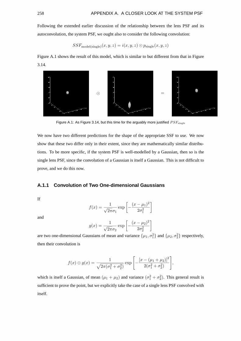
258 APPENDIX A. A CLOSER LOOK AT THE SYSTEM PSF
Following the extended earlier discussion of the relationship between the lens PSF and its
autoconvolution, the system PSF, we ought also to consider the following convolution:
SSFmodel(single)(x, y, z) = i(x, y, z)¯ psingle(x, y, z)
Figure A.1 shows the result of this model, which is similar to but different from that in Figure
3.14.
¯ =
Figure A.1: As Figure 3.14, but this time for the arguably more justified PSFsingle
We now have two different predictions for the shape of the appropriate SSF to use. We now
show that these two differ only in their extent, since they are mathematically similar distribu-
tions. To be more specific, if the system PSF is well-modelled by a Gaussian, then so is the
single lens PSF, since the convolution of a Gaussian is itself a Gaussian. This is not difficult to
prove, and we do this now.
A.1.1 Convolution of Two One-dimensional Gaussians
If
f(x) =1√
2πσ1
exp[−(x− µ1)2
2σ21
]
and
g(x) =1√
2πσ2
exp[−(x− µ2)2
2σ22
]
are two one-dimensional Gaussians of mean and variance{µ1, σ21} and{µ2, σ
22} respectively,
then their convolution is
f(x)¯ g(x) =1√
2π(σ21 + σ2
2)exp
[− [x− (µ1 + µ2)]
2
2(σ21 + σ2
2)
],
which is itself a Gaussian, of mean(µ1 + µ2) and variance(σ21 + σ2
2). This general result is
sufficient to prove the point, but we explicitly take the case of a single lens PSF convolved with
itself.

A.1. SOME REMARKS ON THE MODEL OF THE SYSTEM PSF 259
A.1.2 Convolution of a one-dimensional Gaussian with itself
We are interested in thesystempoint spread function,p(x), which we have assumed is formed
purely by the convolution of thelenspoint spread function,psingle(x) with itself. To recover
the lens PSF from the modelled system PSF requires the followingautoconvolution, which is
obtained straightforwardly from the above:
If
psingle(x) =1√2πσ
exp[−(x− µ)2
2σ2
], (A.1)
then
psingle(x)¯psingle(x) =1√
2π(σ2 + σ2)exp
[− [x− (µ + µ)]2
2(σ2 + σ2)
]=
12σ√
πexp
[− [x− 2µ]2
4σ2
].
(A.2)
This simply states that the autoconvolution ofpsingle(x) having meanµ and varianceσ2 is a
Gaussian of mean2µ and variance4σ2. Since we knowp(x), we can measure triviallyµp ≡ 2µ
andσp ≡ 2σ.
A.1.3 Recovering a Gaussian from its Autoconvolution
For completeness, we also include an example of how to infer the single PSF given the system
PSF. We do this using the converse argument to the above, which allows one to recover the
Gaussian whose autoconvolution is known.
Sincepsingle(x)¯ psingle(x) is identically the system PSF,p(x), and is known, the desired lens
PSF can be recovered in this way.
From A.1 and A.2, we see that
psingle(x)¯ psingle(x)psingle(x)
=1
2σ√
πexp
[− [x− 2µ]2
4σ2
]×√
2πσ exp[(x− µ)2
2σ2
]=
1√2
exp[x2 − 2µ2
4σ2
].
Thus the desired single lens PSF is:
psingle(x) =√
2psingle(x)¯ psingle(x)
exp[
x2−2µ2
4σ2
] .
More neatly, and in terms ofp(x), the known system PSF:
psingle(x) =√
2psingle(x)¯ psingle(x) exp
[−(x2 − µ2
p)2σ2
p
]≡√
2p(x) exp
[−(x2 − µ2
p)2σ2
p
].

260 APPENDIX A. A CLOSER LOOK AT THE SYSTEM PSF
The extension to higher dimensions is straightforward. In three dimensions:
psingle(x, y, z) =√
2p(x, y, z) exp[− 1
2(σxyp )2
[(x2 + y2 − 2µ2
xy)]− (z2 − µ2
z)2(σz
p)2
],
in which we make explicit the assumption that the PSF is identical in the x- and y-directions.
The above rather straightforward mathematics are all of the tools we need to convert between
system and single lens PSF.

List of Figures
1.1 A schematic representation of various sphere packings. . . . . . . . . . . . . . 3
2.1 Ideal hard (monodisperse) sphere pair potential U(r) where r is the centre-
centre separation and R is the particle radius. . . . . . . . . . . . . . . . . . . 12
2.2 Explanation of how g(r) is constructed (left), and a schematic example illus-
trating its important features (right). . . . . . . . . . . . . . . . . . . . . . . . 15
2.3 Schematic illustration of unnormalised version of g(r), which is simply the
number of particles,N(r), found in a spherical shell of thicknessdr and radius
r. The dashed line represents the “ideal gas”r3 dependence. . . . . . . . . . . 16
2.4 The order parameter versus volume fraction plane. The black line is the locus
of jammed states. Point A is the lowest volume fraction jammed structure, B
the close-packed crystal, and MRJ the maximally-random jammed state. Taken
from [43]. . . . . . . . . . . . . . . . . . . . . . . . . . . . . . . . . . . . . . 20
2.5 The hard sphere equation of state. . . . . . . . . . . . . . . . . . . . . . . . . 23
2.6 A schematic phase-diagram for hard spheres. See text for details. . . . . . . . . 24
2.7 A two-dimensional illustration of the mechanism behind entropy-driven freez-
ing of hard spheres. Despite being more ordered, the right-hand system has
higher overall entropy due to its higher free volume entropy. See text for fuller
explanation. . . . . . . . . . . . . . . . . . . . . . . . . . . . . . . . . . . . . 24
2.8 Two types of stabilisation for colloidal particles: charge-stabilisation (left) and
steric stabilisation (right) stabilisation. . . . . . . . . . . . . . . . . . . . . . . 27
261

262 LIST OF FIGURES
2.9 Schematic illustration of interaction potentials for ideal hard spheres (left),
sterically-stabilised colloids (middle) and charge-stabilised colloids (right). From
[60] (see also [61], cited therein). . . . . . . . . . . . . . . . . . . . . . . . . . 28
2.10 A very simple bridge, as argued by Nolan and Kavanagh. Taken from [90]. . . 35
2.11 Nolan and Kavanagh’s explanation of how varying degrees of bridging can
permit sphere packings stable against gravity for a range of volume fraction.
Taken from [90]. . . . . . . . . . . . . . . . . . . . . . . . . . . . . . . . . . 36
2.12 The final volume fraction of a sediment of hard spheres in a solvent can vary
depending on the gravitational Peclet number (∝ ∆g in the Figure). The upper
curve is the relevant one. Taken from [91]. . . . . . . . . . . . . . . . . . . . . 37
2.13 A sample bridge, as an indication of what to expect later in this thesis. . . . . . 38
3.1 The generic imaging process. . . . . . . . . . . . . . . . . . . . . . . . . . . . 44
3.2 Curvature of field . . . . . . . . . . . . . . . . . . . . . . . . . . . . . . . . . 46
3.3 Image magnification by a single lens. . . . . . . . . . . . . . . . . . . . . . . . 52
3.4 The infinite-tube-length compound microscope. . . . . . . . . . . . . . . . . . 54
3.5 Evolutionary stages of Point Scanning Microscopes. . . . . . . . . . . . . . . . 56
3.6 The confocal principle. . . . . . . . . . . . . . . . . . . . . . . . . . . . . . . 58
3.7 The axial elongation of a uniformly-fluorescent sphere. . . . . . . . . . . . . . 60
3.8 A conventional fluorescence microscope. . . . . . . . . . . . . . . . . . . . . . 62
3.9 A schematic diagram of the confocal microscope. . . . . . . . . . . . . . . . . 63
3.10 Isophotes ofI(u, v). . . . . . . . . . . . . . . . . . . . . . . . . . . . . . . . 66
3.11 The Airy pattern in the focal and axial planes . . . . . . . . . . . . . . . . . . 67
3.12 The improvement in resolution due to a confocal microscope. . . . . . . . . . . 69
3.13 Model of the system PSF. . . . . . . . . . . . . . . . . . . . . . . . . . . . . . 72
3.14 Model of a spherical particle (left), the PSF (centre) and the corresponding
image (right). . . . . . . . . . . . . . . . . . . . . . . . . . . . . . . . . . . . 72

LIST OF FIGURES 263
3.15 A comparison of the modelled intensity profile (solid black line) for a2µm
diameter sphere and the measured equivalent for a1µm reference sphere. Data
are shown for the x-, y-, and z-directions (left, middle, right respectively). The
modelled PSF assumes a lateral resolution of300nm and an axial resolution of
600nm. . . . . . . . . . . . . . . . . . . . . . . . . . . . . . . . . . . . . . . 74
3.16 As in Figure 3.15, but this time with the reference sphere artificially doubled in
size. Though not wholly justifiable, the agreement is nonetheless convincing. . 75
3.17 Jabłonski diagram, showing the essential features of the fluorescence and phos-
phorescence phenomena. . . . . . . . . . . . . . . . . . . . . . . . . . . . . . 81
4.1 Images and corresponding histograms to illustrate the effect of offset (top) and
gain (bottom). See text for details. . . . . . . . . . . . . . . . . . . . . . . . . 89
4.2 A saturated image and its histogram. In this case, reducing the offset would
probably be sufficient to rectify the problem adequately; in general both this
and the gain will require to be adjusted. . . . . . . . . . . . . . . . . . . . . . 90
4.3 A sample image of a Richardson Test Slide, showing the case of a badly dis-
torted image. Such distortions are surprisingly difficult to see in images of
colloidal samples. . . . . . . . . . . . . . . . . . . . . . . . . . . . . . . . . . 92
4.4 Confocal micrograph coordinate system definition. . . . . . . . . . . . . . . . 93
4.5 The convolution of the noise-suppressing gaussian kernel,Aλn , with the above
delta function (left) illustrates its form. The Fourier Transform of this image
(right) is, to within a constant (= α in text), the Fourier Transform of the kernel. 100
4.6 As above, but this time for the smoothing ‘boxcar’ kernel,Aw. . . . . . . . . . 100
4.7 A typical confocal micrograph before processing, and its Fourier Transform. . . 101
4.8 Original image having been filtered using the two-dimensional algorithm (left),
and its Fourier Transform (right). . . . . . . . . . . . . . . . . . . . . . . . . . 101
4.9 A border of appropriate size (left), and its Fourier Transform (right). . . . . . . 102
4.10 The original image having been filtered using the three-dimensional algorithm
(left), and its Fourier Transform (right). . . . . . . . . . . . . . . . . . . . . . 103
4.11 An example of a reconstruction based on particle coordinates. . . . . . . . . . 112

264 LIST OF FIGURES
4.12 A typical two-dimensional slice from a sediment with crosses overlaid at the
particle locations. . . . . . . . . . . . . . . . . . . . . . . . . . . . . . . . . . 113
4.13 Two example clouds showing radius of gyration squared, and peak and inte-
grated brightness. . . . . . . . . . . . . . . . . . . . . . . . . . . . . . . . . . 114
4.14 Histograms of the fractional part of the coordinates in x, y, and z. . . . . . . . . 115
4.15 The colour code used to illustrate changes in the rdf for various centroid tech-
nique parameters. . . . . . . . . . . . . . . . . . . . . . . . . . . . . . . . . . 118
4.16 The effect of varying the “extent” parameter on detected particles. . . . . . . . 118
4.17 The effect of the noise filter size on the particle coordinates for the centroid
method. . . . . . . . . . . . . . . . . . . . . . . . . . . . . . . . . . . . . . . 120
4.18 The effect of varying the “separation” parameter on the determined particle
coordinates using the centroid method. . . . . . . . . . . . . . . . . . . . . . . 121
4.19 The effect of varying the “threshold” parameter on the determined particle co-
ordinates using the centroid method. . . . . . . . . . . . . . . . . . . . . . . . 121
4.20 The simulated intensity profile through a single particle. . . . . . . . . . . . . . 124
4.21 The effect of overlapping SSFs on the centroid position. . . . . . . . . . . . . . 125
4.22 The simulated intensity profile through two particles in contact (lateral and axial).125
4.23 The simulated intensity profile for vertically-stacked but separated particles. . . 126
4.24 Comparison radial distribution functions for “good” and “bad” glassy samples
found using the centroid algorithm. . . . . . . . . . . . . . . . . . . . . . . . . 129
4.25 Slices through the chi-square hypersurface. . . . . . . . . . . . . . . . . . . . 133
4.26 Two-dimensional projections of the Chi-square hypersurface. . . . . . . . . . . 133
4.27 Chi-square at sub-pixel lattice points. . . . . . . . . . . . . . . . . . . . . . . 135
4.28 Chi-square hypersurface as shown in Figure 4.25. . . . . . . . . . . . . . . . . 135
4.29 A crude error estimate for the chi-square fitting procedure. . . . . . . . . . . . 136
4.30 The improvement in g(r) for a high quality image of a glassy sample. . . . . . . 137
4.31 The improvement in g(r) for a mediocre quality image of a glassy sample. . . . 138

LIST OF FIGURES 265
4.32 Improvement in g(r) for samples of different refractive index mismatch be-
tween solvent and particles. . . . . . . . . . . . . . . . . . . . . . . . . . . . . 139
4.33 The effect of overlapping SSFs on chi-square. . . . . . . . . . . . . . . . . . . 140
4.34 A schematic illustration demonstrating howχ2B might work. . . . . . . . . . . 141
4.35 Theχ2B measure does does not appear to produce a significant improvement in
g(r). . . . . . . . . . . . . . . . . . . . . . . . . . . . . . . . . . . . . . . . . 142
4.36 The improvement in g(r) caused by discarding any particles with a poorχ2 value.144
5.1 An undyed PMMA sphere in a fluorescent solvent. . . . . . . . . . . . . . . . 149
5.2 Triangulation in 2d and 3d. . . . . . . . . . . . . . . . . . . . . . . . . . . . . 159
5.3 Voronoı diagram for particles (2d). . . . . . . . . . . . . . . . . . . . . . . . . 160
5.4 Illustration of how inclusion of particles which do not genuinely belong to the
bulk sample skew the distribution of Voronoı volumes. . . . . . . . . . . . . . 161
5.5 Sample Cell 1 . . . . . . . . . . . . . . . . . . . . . . . . . . . . . . . . . . . 165
5.6 Adhesive application . . . . . . . . . . . . . . . . . . . . . . . . . . . . . . . 167
5.7 Sample Cell 2 . . . . . . . . . . . . . . . . . . . . . . . . . . . . . . . . . . . 169
5.8 Oil immersion lens. . . . . . . . . . . . . . . . . . . . . . . . . . . . . . . . . 170
6.1 The Ross Bridge at Comrie, Perthshire. . . . . . . . . . . . . . . . . . . . . . 172
6.2 In two dimensions, a stable particle and an unstable particle. . . . . . . . . . . 173
6.3 Even in two dimensions, a stable particle can be stabilised by more than one
subset. . . . . . . . . . . . . . . . . . . . . . . . . . . . . . . . . . . . . . . . 173
6.4 The criterion for stability in three dimensions. . . . . . . . . . . . . . . . . . . 174
6.5 A cartoon of a humpback bridge, in which particles2, 3, 4, 5, and6 are involved
in mutual stabilisations. . . . . . . . . . . . . . . . . . . . . . . . . . . . . . . 174
6.6 Mutually stabilising particles in two dimensions (left) and three dimensions
(right). Smaller base particles have been shown in the three dimensional case
for clarity. . . . . . . . . . . . . . . . . . . . . . . . . . . . . . . . . . . . . . 175

266 LIST OF FIGURES
6.7 In the case of polydisperse particles, the separation of centres is different for
each pair of particles. . . . . . . . . . . . . . . . . . . . . . . . . . . . . . . . 176
6.8 For particles whose centres are too close together, the condition for kissing
neighbours is altered, but still captures . . . . . . . . . . . . . . . . . . . . . . 177
6.9 Determined coordination number with capture criterion. . . . . . . . . . . . . . 186
6.10 Proportion of particles deemed stable for increasing capture criterion. . . . . . 187
6.11 Proportion of particles deemed rattlers with increasing caption criterion. . . . . 187
6.12 Proportion of particles deemed to be stabilised by precisely one stabilising sub-
set, with increasing capture criterion. . . . . . . . . . . . . . . . . . . . . . . . 188
6.13 Mean number of stabilising subsets per stable particle with increasing capture
criterion. . . . . . . . . . . . . . . . . . . . . . . . . . . . . . . . . . . . . . . 189
6.14 Mean number of stabilising particles per stable particle, with increasing capture
criterion. . . . . . . . . . . . . . . . . . . . . . . . . . . . . . . . . . . . . . . 189
6.15 Ratio of the mean number of stabilising subsets per stable particle to the mean
number of stabilising particles per stable particle, with increasing capture cri-
terion. . . . . . . . . . . . . . . . . . . . . . . . . . . . . . . . . . . . . . . . 190
6.16 Bridge distributions for increasing capture criterion using the LCOM method
for deciding upon stabilisations. . . . . . . . . . . . . . . . . . . . . . . . . . 191
6.17 Bridge distributions for increasing capture criterion using the LSSQ method
for deciding upon stabilisations. . . . . . . . . . . . . . . . . . . . . . . . . . 191
6.18 Bridge distributions for increasing capture criterion: comparison between LCOM
and LSSQ methods for deciding upon stabilisations. . . . . . . . . . . . . . . . 192
6.19 Mean bridge size with increasing capture criterion for LSSQ and LCOM. . . . 192
6.20 Maximum bridge size with increasing capture criterion for LSSQ (top, black)
and LCOM (bottom, red). . . . . . . . . . . . . . . . . . . . . . . . . . . . . . 193
7.1 Relationship between the nominal (i.e. intended) volume fraction and the ac-
tual volume fraction. . . . . . . . . . . . . . . . . . . . . . . . . . . . . . . . 198

LIST OF FIGURES 267
7.2 Pair correlation functions for all decalin samples with nominal volume frac-
tions0.40 to 0.64. . . . . . . . . . . . . . . . . . . . . . . . . . . . . . . . . . 199
7.3 The position of the first peak in the radial distribution function as a function of
volume fraction. . . . . . . . . . . . . . . . . . . . . . . . . . . . . . . . . . 200
7.4 Relationship between coordination number and volume fraction. . . . . . . . . 202
7.5 A cubic polynomial fit to allow approximate conversion between mean coordi-
nation number at1.1 diameters and the volume fraction. . . . . . . . . . . . . 202
7.6 Evolution of volume fraction with time, for each sample. . . . . . . . . . . . . 203
7.7 Fits to volume fraction with time. . . . . . . . . . . . . . . . . . . . . . . . . . 204
7.8 Evolution of coordination number with time. . . . . . . . . . . . . . . . . . . 206
7.9 Evolution ofg(r) for a sample of initial volume fractionΦi = 0.42 as it sedi-
ments. . . . . . . . . . . . . . . . . . . . . . . . . . . . . . . . . . . . . . . . 207
7.10 Evolution ofg(r) for a sample of initial volume fractionΦi = 0.42. . . . . . . 207
7.11 A representative slice in the x-z direction, which appears to show a preference
for a particular direction in the sample. . . . . . . . . . . . . . . . . . . . . . . 209
7.12 Proportion of particles deemed stable in samples of increasing packing density. 210
7.13 Proportion of particles deemed to be unstable in samples of increasing packing
density. . . . . . . . . . . . . . . . . . . . . . . . . . . . . . . . . . . . . . . 212
7.14 A representation of the spatial distribution of unstable particles for samples in
the rangeΦ = 0.64 (top left) to0.45 (bottom right). . . . . . . . . . . . . . . . 213
7.15 Spatial distribution of unstable particles for samples of volume fractionΦ =
0.64, 0.60, 0.51, and0.45 (top to bottom). . . . . . . . . . . . . . . . . . . . . 214
7.16 Mean number of stabilising particles per stable particle for samples of increas-
ing packing density. . . . . . . . . . . . . . . . . . . . . . . . . . . . . . . . 216
7.17 Mean number of stabilising subsets per stable particle for samples of increasing
packing density. . . . . . . . . . . . . . . . . . . . . . . . . . . . . . . . . . . 217
7.18 Ratio of mean number of stabilising particles to mean number of stabilising
subsets per stable particle. . . . . . . . . . . . . . . . . . . . . . . . . . . . . 218

268 LIST OF FIGURES
7.19 Proportion of particles deemed to be stabilised be precisely one subset in sam-
ples of increasing packing density. . . . . . . . . . . . . . . . . . . . . . . . . 219
7.20 Bridge size distribution for samples of increasing packing density (samples as
given in Table 7.1). The lowest density samples are shown in red (beginning
with nominalΦ = 0.40), and as the volume fraction increases toΦ = 0.64,
the curves move upwards (and change from red to blue to light blue. The last
curve is black, and has nominalΦ = 0.64. The right-hand image shows the
same data, but this time with a result from the granular case superimposed in
green. This is the highest curve. . . . . . . . . . . . . . . . . . . . . . . . . . 220
7.21 Bridge size distribution for samples of increasing packing density, this time
normalised to the number of stable particles. . . . . . . . . . . . . . . . . . . 221
7.22 Mean bridge size for samples of increasing packing density. . . . . . . . . . . 222
7.23 Maximum bridge size for samples of increasing packing density. . . . . . . . . 222
7.24 The effect of rotation on the distribution of bridge sizes. . . . . . . . . . . . . . 223
8.1 Relationship between the nominal (i.e. intended) volume fraction and the ac-
tual volume fraction for the density-matched samples. . . . . . . . . . . . . . . 227
8.2 A phase diagram for the density-matched particles. . . . . . . . . . . . . . . . 227
8.3 The colour code used to distinguish between density-matched samples. As
indicated, the high volume fraction samples are “bluest”. . . . . . . . . . . . . 228
8.4 The radial distribution functions for density-matched samples with volume
fraction in the range'0.40-0.60. . . . . . . . . . . . . . . . . . . . . . . . . . 228
8.5 The position of the first peak in the radial distribution function as a function of
volume fraction. . . . . . . . . . . . . . . . . . . . . . . . . . . . . . . . . . . 229
8.6 The relationship between coordination number and measured volume fraction
for the density-matched samples. . . . . . . . . . . . . . . . . . . . . . . . . . 230
8.7 The evolution of the sample volume fraction (in time) for density-matched sam-
ples at a range of initial densities. . . . . . . . . . . . . . . . . . . . . . . . . . 232
8.8 The evolution of the mean coordination number in time for density-matched
samples at a range of initial densities. . . . . . . . . . . . . . . . . . . . . . . 232

LIST OF FIGURES 269
8.9 The evolution of g(r) for a density-matched sample of initial volume fraction
Φi = 0.45. . . . . . . . . . . . . . . . . . . . . . . . . . . . . . . . . . . . . 233
8.10 The evolution of g(r) for a density-matched sample of initial volume fraction
Φi = 0.51. . . . . . . . . . . . . . . . . . . . . . . . . . . . . . . . . . . . . 233
8.11 The evolution of g(r) for a density-matched sample of initial volume fraction
Φi = 0.54. . . . . . . . . . . . . . . . . . . . . . . . . . . . . . . . . . . . . 234
8.12 The evolution of g(r) for a density-matched sample of initial volume fraction
Φi = 0.59. . . . . . . . . . . . . . . . . . . . . . . . . . . . . . . . . . . . . 234
8.13 Proportion of particles deemed stable in samples of increasing packing density
with volume fraction and coordinate number for both the density-matched and
non-density-matched samples. . . . . . . . . . . . . . . . . . . . . . . . . . . 235
8.14 Proportion of particles deemed unstable in samples of increasing packing den-
sity with volume fraction and coordinate number for both the density-matched
and non-density-matched samples. . . . . . . . . . . . . . . . . . . . . . . . . 235
8.15 Number of stabilising particles per stable particle in samples of increasing
packing density with volume fraction and coordinate number for both the density-
matched and non-density-matched samples. . . . . . . . . . . . . . . . . . . . 237
8.16 Number of stabilising subsets per stable particle in samples of increasing pack-
ing density with volume fraction and coordinate number for both the density-
matched and non-density-matched samples. . . . . . . . . . . . . . . . . . . . 238
8.17 Ratio of the number of stabilising subsets per stable particle to the number
of stabilising particles in samples of increasing packing density with volume
fraction and coordinate number for both the density-matched and non-density-
matched samples. . . . . . . . . . . . . . . . . . . . . . . . . . . . . . . . . . 239
8.18 Proportion of stable particles which were stabilised by precisely one subset
in samples of increasing packing density with volume fraction and coordinate
number for both the density-matched and non-density-matched samples. . . . . 239
8.19 A comparison of the bridge size distribution for both the density-matched re-
sults (left), and decalin-only results (right). . . . . . . . . . . . . . . . . . . . 241

270 LIST OF FIGURES
8.20 A comparison of decalin-only bridges and the density-matched bridges, indi-
cating the point at which the bridge size distribution departs from the apparent
family of curves evident for samples of higher mean coordination number. . . . 241
8.21 Mean bridge size with increasing sample density with volume fraction and co-
ordinate number for both the density-matched and non-density-matched samples.242
8.22 Maximum bridge size with increasing sample density with volume fraction for
both the density-matched and non-density-matched samples. . . . . . . . . . . 243
8.23 Dynamic phase diagram for five particle sizes, as found by Lootenset al.. . . . 246
A.1 As Figure 3.14, but this time for the arguably more justifiedPSFsingle . . . . . 258

List of Tables
1.1 Types of colloids with some familiar examples. . . . . . . . . . . . . . . . . . 4
1.2 Some examples of granular materials. . . . . . . . . . . . . . . . . . . . . . . 6
4.1 A colour code for Figures 4.16-4.19 . . . . . . . . . . . . . . . . . . . . . . . 119
6.1 Pseudo-code for Bridge Finder main program. . . . . . . . . . . . . . . . . . 176
6.2 Pseudo-code for Bridge Finder Step 4. . . . . . . . . . . . . . . . . . . . . . . 178
7.1 Initial volume fractions of samples prepared. . . . . . . . . . . . . . . . . . . . 196
7.2 The times at which stacks were captured during long time series. Times vary
slightly between experiments, up to around±3 seconds at the higher times, but
much lower for earlier stacks. . . . . . . . . . . . . . . . . . . . . . . . . . . . 197
7.3 Some values of N andNC3. . . . . . . . . . . . . . . . . . . . . . . . . . . . . 217
8.1 Initial volume fractions of density-matched samples prepared. . . . . . . . . . 226
271

272 LIST OF TABLES
Bibliography
[1] T. Aste and D. L. Weaire.The Pursuit of Perfect Packing. Institute of Physics, 2000.
[2] T. Hales. What have Kepler, Hilbert, Milnor, Coxeter, Fejes Toth and others said aboutthe Kepler conjecture? http://www.math.pitt.edu/˜thales/kepler98/.
[3] J.D. Bernal. The Bakerian Lecture, 1962: The structure of liquids.Proc. Royal. Soc.,A280:299–321, 1964.
[4] W.G. Hoover and F.H. Ree. Melting transition and communal entropy for hard spheres.J.Chem.Phys., 49:3609–3617, 1968.
[5] V. Martelozzo.Crystallisation and Phase Separation in Colloidal Systems. PhD thesis,University of Edinburgh School of Physics, 2001.
[6] D. Frenkel. Playing tricks with designer “atoms”.Science, 296:65–66, 2002.
[7] M.D. Haw. http://www.middle-world.com/. Also see forthcoming book “Middle World”by Macmillan.
[8] P.-G. de Gennes. Granular matter: a tentative view.Rev. Mod. Phys., 71:S374–S382,1999.
[9] M.E. Cates, J.P. Wittmer, J.-P. Bouchaud, and P. Claudin. Jamming, force chains andfragile matter.Phys. Rev. Lett., 81:1841, 1998.
[10] Purdue University Particulate Systems Laboratory.http://widget.ecn.purdue.edu/ psl/background/.
[11] J. Kepler.Strena, The six-cornered snowflake.G. Tampach, Frankfurt am Main, 1611.
[12] J.D. Bernal. A geometrical approach to the structure of liquids.Nature, 183:141–147,1959.
[13] J.D. Bernal. Geometry of the structure of monatomic liquids.Nature, 185:68–70, 1960.
[14] J.D. Bernal and J. Mason. Co-ordination of randomly packed spheres.Nature, 188:910–911, 1960.
[15] J.D. Bernal, I.A. Cherry, J.L. Finney, and K.R. Knight. An optical machine for measur-ing sphere coordinates in random packings.J. Phys. E: Sci. Instr., 3:388–390, 1970.
[16] J.D. Bernal, F.R. Knight, and I. Cherry. Growth of crystals from random close packing.Nature, 202:852–854, 1964.
273

274 BIBLIOGRAPHY
[17] J.D. Bernal and J.L.Finney. Random close packing and the heats of fusion of argon athigh pressures.Nature, 215:269–270, 1967.
[18] G.D. Scott. Radial distribution of the random close packing of equal spheres.Nature,194:956–957, 1962.
[19] G.D. Scott and D.L. Mader. Angular distribution of random close-packed equal spheres.Nature, 188:382–383, 1964.
[20] G. Mason. Radial distribution functions from small packings of spheres.Nature,217:733–735, 1968.
[21] J.L. Finney. Random packings and the structure of simple liquids. i. the geometry ofrandom close packing.Proc. Royal Soc. London A, 319:479–493, 1970.
[22] J.L. Finney and J.D. Bernal. Random close packing and the heats of fusion of simpleliquids. Nature, 213:1079–1082, 1967.
[23] J.G. Berryman. Random close packing of hard spheres and disks.Phys. Rev. A, 27:1053–1061, 1983.
[24] P. Meakin and A.T. Skjeltorp. Application of experimental and numerical methods tothe physics of multiparticle systems.Adv. Phys., 42:1–127, 1993.
[25] E.M. Tory, N.A. Cochrane, and S.R. Waddell. Anisotropy in simulated random packingof equal spheres.Nature, 220:1023–1024, 1968.
[26] E.M. Tory, N.A. Cochrane, and S.R. Waddell. Simulated random packing of equalspheres.Can. J. Chem. Eng., 51:484–493, 1973.
[27] W.S. Jodrey and E.M. Tory. Computer simulation of close random packing of equalspheres.Phys. Rev. A, 32:2347–2351, 1985.
[28] W.S. Jodrey and E.M. Tory. Computer simulation of isotropic, homogeneous, denserandom packing of equal spheres.Powder Technol., 30:111–118, 1981.
[29] B.D. Lubachevsky. How to simulate billiards and similar systems.J. Comp. Phys.,94:255–283, 1991.
[30] B.D. Lubachevsky and F.H. Stillinger. Geometric properties of random disk packings.J. Stat. Phys., 60:561–583, 1990.
[31] B.D. Lubachevsky, F.H. Stillinger, and E.N. Pinson. Disks vs. spheres: Contrastingproperties of random packings.J. Stat. Phys., 64:501–524, 1991.
[32] M.C. Jenkins. Notes on the Lubachevsky-Stillinger algorithm.http://www.ph.ed.ac.uk/˜mjenkins/lubstillstandalone.pdf.
[33] G.D. Scott. Packing of spheres.Nature, 188:908–909, 1960.
[34] F.P. Preparata and M.I. Shamos.Computational Geometry: An Introduction. Springer-Verlag New York Inc., 1993.
[35] P.J. Steinhardt, D.R. Nelson, and M. Ronchetti. Bond-orientational order in liquids andglasses.Phys. Rev. B, 28:784–805, 1983.

BIBLIOGRAPHY 275
[36] P. R. ten Wolde, M. J. Ruiz-Montero, and D. Frenkel. Numerical calculation of therate of crystal nucleation in a lennard-jones system at moderate undercooling.J. Chem.Phys., 104:9932, 1996.
[37] U. Gasser, E.R. Weeks, A.B. Schofield, P.N. Pusey, and D.A. Weitz. Real space imagingof nucleation and growth in colloidal crystallization.Science, 292:258–262, 2001.
[38] U. Gasser, A.B. Schofield, and D.A. Weitz. Local order in a supercooled colloidal fluidobserved by confocal microscopy.J. Phys.: Condens. Matter, 15:S375–S380, 2003.
[39] H. Reiss. Statistical geometry in the study of fluids and porous media.J. Phys. Chem.,96:4736, 1992.
[40] R.M.L. Evans and M.D. Haw. Correlation length by measuring empty space in simulatedaggregates.Europhys. Lett., 60:404–410, 2002.
[41] M.D. Haw. Void structure and cage dynamics in concentrated suspensions.cond-mat/0511464, 2005.
[42] S. Torquato.Random Heterogeneous Materials: Microstucture and Macroscopic Prop-erties. Springer-Verlag, 2002.
[43] S. Torquato, T.M. Truskett, and P.G. Debenedetti. Is random close packing of sphereswell defined?Phys. Rev. Lett., 84:2064–2067, 2000.
[44] Nature Molecular Physics Correspondent (Unnamed). What is random packing?Nature,239:488, 1972.
[45] G.D. Scott and D.M. Kilgour. The density of random close packing of spheres.Br. J.Appl. Phys., 2:863, 1969.
[46] T.M. Truskett, S. Torquato, and P.G. Debenedetti. Towards a quantification of disorder inmaterials: Distinguishing equilibrium and glassy sphere packings.Phys. Rev. E, 62:993–1001, 2000.
[47] C.S. O’Hern, S.A. Langer, A.J. Liu, and S.R. Nagel. Random packings of frictionlessparticles.Phys. Rev. Lett., 88:075507, 2002.
[48] C.S. O’Hern, L.E. Silbert, A.J. Liu, and S.R. Nagel. Jamming at zero temperature andzero applied stress: The epitome of disorder.Phys. Rev. E, 68:011306, 2003.
[49] A. Donev, S. Torquato, F.H. Stillinger, and R. Connelly. Comment on “jamming at zerotemperature and zero applied stress: The epitome of disorder”.Phys. Rev. E, 70:043301,2004.
[50] C.S. O’Hern, L.E. Silbert, A.J. Liu, and S.R. Nagel. Reply to “comment on jammingat zero temperature and zero applied stress: The epitome of disorder”.Phys. Rev. E,70:043302, 2004.
[51] W.W. Wood and J.D. Jacobson. Preliminary results from a recalculation of the montecarlo equation of state of hard spheres.J. Chem. Phys., 27:1207, 1957.
[52] N.F. Carnahan and K.E. Starling. Equation of state for non-attracting rigid spheres.J.Chem. Phys., 51:635–636, 1969.

276 BIBLIOGRAPHY
[53] L. Woodcock. Glass transition in the hard-sphere model and Kauzmann’s paradox.Ann.N.Y. Acad. Sci., 371:274–298, 1981.
[54] K.R. Hall. Another hard-sphere equation of state.J.Chem.Phys., 57:2252–2254, 1972.
[55] J. Israelachvili.Intermolecular and Surface Forces. Academic Press, London, 1991.
[56] P.N. Pusey.Colloidal Suspensions, in Liquids, Freezing and Glass Transition (pp. 763-942). Elsevier, Amsterdam. 1991.
[57] M. S. Elliot. The Optical Microscopy of Colloidal Suspensions. PhD thesis, Universityof Edinburgh School of Physics, 1999.
[58] A. Vrij. Polymer at interfaces and the interaction in colloidal dispersions.Pure Appl.Chem., 48:471–483, 1976.
[59] P.-G. de Gennes.Adv. Colloid Interface Sci., 27:189, 1987.
[60] H. Sedgwick.Colloidal Metastability. PhD thesis, University of Edinburgh School ofPhysics, 2003.
[61] A.K. Sood. Structural ordering in colloidal suspensions.Solid State Physics, 45:1, 1991.
[62] J.-P. Hansen and D. Schiff. Influence of interatomic repulsion on the structure of liquidsat melting.Mol. Phys., 25:1281–1290, 1973.
[63] D. J. Fairhurst.Polydispersity in Colloidal Phase Transitions. PhD thesis, University ofEdinburgh School of Physics, 1999.
[64] Y.S. Papir and I.M. Krieger. Rheological studies on dispersions of uniform colloidalspheres: Ii. dispersions in nonaqueous media.J. Colloid Interface Sci., 34:126–130,1970.
[65] C. de Kruif, E. Israel, A. Vrij, and W. Russel. Hard-sphere colloidal dispersions—viscosity as a function of shear rate and volume fraction.J. Chem. Phys., 83:4717–4725,1985.
[66] P.N. Pusey and W. van Megan. Phase behaviour of concentrated suspensions of nearlyhard colloidal spheres.Nature, 320:340–342, 1986.
[67] R.J. Speedy. On the reproducibilty of glasses.J. Chem. Phys., 100:6684–6691, 1994.
[68] R.J. Speedy. The hard sphere glass transition.Mol. Phys., 95:169–178, 1998.
[69] M. Robles, M. Lopez de Haro, A. Santos, and S. Bravo Yuste. Is there a glass transitionfor dense hard-sphere systems?J. Chem. Phys., 108:1290–1291, 1998.
[70] S. Torquato. Private communication.
[71] University of Queensland. The pitch drop experiment.http://www.physics.uq.edu.au/pitchdrop/pitchdrop.shtml.
[72] C. A. Angell. Formation of glasses from liquids and biopolymers.Science, 267:1924,1995.

BIBLIOGRAPHY 277
[73] J. Zhu, M. Li, W. Meyer, R. H. Ottewill, STS-73 Space Shuttle Crew, W. B. Russel, andP. M. Chaikin. Crystallization of hard sphere colloids in microgravity.Nature, 387:883,1997.
[74] W. K. Kegel. Crystallization in glassy suspensions of colloidal hard spheres.Langmuir,16:939–941, 2000.
[75] G. Adam and J. H. Gibbs.J. Chem. Phys., 43:139, 1965.
[76] A. van Blaaderen and P. Wiltzius. Real-space structure of colloidal hard-sphere glasses.Science, 270:1177–1179, 1995.
[77] E. R. Weeks, J. C. Crocker, A. C. Levitt, A.B. Schofield, and D. A. Weitz. Three-dimensional direct imaging of structural relaxation near the colloidal glass transition.Science, 287:627–631, 2000.
[78] E.R. Weeks and D.A. Weitz. Properties of cage rearrangements observed near the col-loidal glass transition.Phys. Rev. Lett., 89:095704, 2002.
[79] E.R. Weeks and D.A. Weitz. Subdiffusion and the cage effect studied near the colloidalglass transition.Chemical Physics, 284:361, 2002.
[80] R.E. Courtland and E.R. Weeks. Direct visualization of ageing in colloidal glasses.J.Phys.: Condens. Matter, 15:S359–S365, 2003.
[81] J. Geng, D. Howell, E. Longhi, R.P. Behringer, G. Reydellet, L. Vanel, E. Clement, andS. Luding. Footprints in sand: The response of a granular material to local perturbations.Phys. Rev. Lett., 87:035506, 2001.
[82] O. Reynolds.Philos. Mag., 20:469, 1885.
[83] H.M. Jaeger and S.R. Nagel. Physics of the granular state.Science, 255:1523–1531,1992.
[84] S.F. Edwards and D.V. Grinev. Granular physics as a physics problem.Adv. ComplexSystems, 4:1–17, 2001.
[85] S.F. Edwards and D.V. Grinev.Statistical Physics of the Jamming Transition: The Searchfor Simple Models. Taylor and Francis, New York, 2001.
[86] A. Mehta and G.C. Barker. Vibrated powders: A microscopic approach.Phys. Rev. Lett.,67:394–397, 1991.
[87] G.C. Barker and A. Mehta. Vibrated powers: Structure, correlations, and dynamics.Phys. Rev. A, 45:3435–3446, 1992.
[88] G.C. Barker and A. Mehta. Transient phenomena, self-diffusion, and orientational ef-fects in vibrated powders.Phys. Rev. E, 47:184–188, 1993.
[89] A. Mehta and G.C. Barker. The dynamics of sand.Rep. Prog. Phys., 57:383–416, 1994.
[90] G.T. Nolan and P.E. Kavanagh. Computer simulation of random packing of hard spheres.Powder Technol., 72:149–155, 1992.
[91] G.Y. Onoda and E.G. Liniger. Random loose packings of uniform spheres and the dila-tancy onset.Phys. Rev. Lett., 64:27272730, 1990.

278 BIBLIOGRAPHY
[92] R. Blumenfeld, S.F. Edwards, and R.C. Ball. Granular matter and the marginal rigiditystate.J. Phys.: Condens. Matter, 17:S2481–S2487, 2005.
[93] E. A. J. F. Peters, M. Kollmann, T.M.A.O.M. Barenbrug, and A.P. Philipse. Caging of ad-dimensional sphere and its relevance for the random dense sphere packing.Phys. Rev.E, 63:021404, 2001.
[94] A.P. Philipse. Caging effects in amorphous hard-sphere solids.Colloids Surf., A,213:167–173, 2003.
[95] L.A. Pugnaloni, G.C. Barker, and A. Mehta. Multi-particle structures in non-sequentially reorganized hard sphere deposits.Adv. Complex Systems, 4:289–297, 2001.
[96] L.A. Pugnaloni and G.C. Barker. Structure and distribution of arches in shaken hardsphere deposits.Physica A, 337:428–442, 2004.
[97] A. Mehta, G.C. Barker, and J.M. Luck. Cooperativity in sandpiles: statistics of bridgegeometries.J. Stat. Phys., P10014:1–15, 2004.
[98] A. Mehta. Competition and cooperation: aspects of dynamics in sandpiles.J. Phys.:Condens. Matter, 17:S2657–S2687, 2005.
[99] K.E. Davis, W.B. Russel, and W.J. Glantschnig. Disorder-to-order transition in settlingsuspensions of colloidal silica: X-ray measurements.Science, 245:507–510, 1989.
[100] J.P. Hoogenboom, D. Derks, P. Vergeer, and A. van Blaaderen. Stacking faults in col-loidal crystals grown by sedimentation.J. Chem. Phys., 117:11320–11328, 2002.
[101] A. Mehta and G.C. Barker. Glassy dynamics in granular compaction.J. Phys.: Condens.Matter, 12:6619–6628, 2000.
[102] A.J. Liu and S.R. Nagel. Jamming is not just cool any more.Nature, 396:21–22, 1998.
[103] A.J. Liu and S.R. Nagel.Jamming and Rheology. Taylor and Francis, 2001.
[104] V. Trappe, V. Prasad, L. Cipelletti, P.N. Segre, and D.A. Weitz. Jamming phase diagramfor attractive particles.Nature, 411:772–773, 2001.
[105] C.B. Holmes.The Jamming of Dense Suspensions Under Imposed Stress. PhD thesis,University of Edinburgh School of Physics, 2004.
[106] M. Pluta. Advanced Light Microscopy Volume 1: Principles and Basic Properties. El-sevier, 1988.
[107] M. Born and E. Wolf.Principles of Optics. Pergamon Press, 1959.
[108] P. Artal, L. Chen, E.J. Fernandez, B. Singer, S. Manzanera, and D.R. Williams. Neuralcompensation for the eyes optical aberrations.J. Vision, 4:281–287, 2004.
[109] Wikipedia. Nyquist-Shannon sampling theorem. http://www.en.wikipedia.org/.
[110] H. Nyquist. Certain topics in telegraph transmission theory.Trans. AIEE, 47:617–644,1928.
[111] C.E. Shannon. Communication in the presence of noise.Proc. Institute of Radio Engi-neers, 37:10–21, 1949.

BIBLIOGRAPHY 279
[112] T. Wilson.Confocal Microscopy. Academic Press, 1990.
[113] W. Lukosz. Optical systems with resolving powers exceeding the classical limit.J. Opt.Soc. Am., 56:1463–1472, 1966.
[114] E.R. Weeks. How does a confocal microscope work?http://www.physics.emory.edu/˜weeks/confocal/.
[115] D. Semwogerere and E. Weeks. Confocal microscopy. to be published in Encylopediaof Biomaterials and Biomedical Engineering, Taylor and Francis, 2005. As referencedin http://www.physics.emory.edu/˜weeks/confocal/.
[116] J.B. Pawley, editor.Handbook of Biological Confocal Microscopy. Plenum Press, 1995.
[117] E. Lommel. Die beugungserscheinungen einer kreisrunden oeffnung und eines kreisnun-den schirmchens theoretisch und experimentell bearbeitet.Abh. Bayer. Akad., 15:233,1885.
[118] J.C. Crocker and D.G. Grier. Methods of digital video microscopy for colloidal studies.J. Colloid Interface Sci., 179:298–310, 1996.
[119] M. Kerker.Scattering of Light. New York, Academic, 1969.
[120] J. Baumgartl and C. Bechinger. On the limits of digital video microscopy.Europhys.Lett., 71:487–493, 2005.
[121] W.J. Hossack. Digital image analysis. University of Edinburgh School of Physics, SeniorHonours Course.
[122] R. C. Gonzalez and R. E. Woods.Digital Image Processing. Addison-Wesley, 1992.
[123] G.G. Stokes. On the change of refrangibility of light.Phil. Trans. Royal Soc. London,142:463–562, 1852.
[124] European Advanced Light Microscopy Network (EAMNET). Photobleaching.http://www.embl.de/eamnet/frap/html/photobleaching.html/, 2004.
[125] Imaging Technology Group. Photobleaching. http://www.itg.uluc.edu/publications/techreports/99-006/photobleaching.htm/.
[126] N.B. Simeonova and W.K. Kegel. Real-space fluorescence recovery after photo bleach-ing of concentrated suspensions of hard colloidal spheres.Faraday Discuss., 123:27,2003.
[127] US Federal Aviation Administration Human Factors Awareness Web Course. The visi-ble spectrum. http://www.hf.faa.gov/Webtraining/VisualDisplays/HumanVisSys2a.htm,Visited August 2005.
[128] TV Technology. Color perception. http://www.tvtechnology.com/features/Tech-Corner/f-rh-color.shtml, Visited August 2005.
[129] Toshiba Imaging Systems Group. Glossary of terms–color depth.http://www.toshiba.com/taisisd/isdsvc/dsglosry.shtml, Visited August 2005.
[130] G. D’Agostini. Bayesian inference in processing experimental data: principles and basicapplications.Rep. Prog. Phys., 66:1383–1419, 2003.

280 BIBLIOGRAPHY
[131] V. Dose. Bayesian inference in physics: case studies.Rep. Prog. Phys., 66:1421–1461,2003.
[132] M. Raffel, C. Willert, and J. Kompenhans.Particle Image Velocimetry–a practical guide.Springer-Verlag, Berlin Heidelberg, 1998.
[133] A.I. Campbell and P. Bartlett. Fluorescent hard-sphere polymer colloids for confocalmicroscopy.J. Colloid Interface Sci., 256:325–330, 2002.
[134] C.P. Royall, M.E. Leunissen, and A. van Blaaderen. A new colloidal model system tostudy long-range interactions quantitatively in real space.J. Phys.: Condens. Matter,15:S3581–S3596, 2003.
[135] J. Bolinder. On the accuracy of a digital particle image velocimetry system. Techni-cal Report ISSN 0282-1990, Institutionen for varme- och kraftteknik, Lund Institute ofTechnology, 1999.
[136] C.A. Murray and D.G. Grier. Video microscopy of monodisperse colloidal systems.Annu. Rev. Phys. Chem., 47:421–462, 1996.
[137] T. Schlicke. PhD thesis, University of Edinburgh School of Physics, 2002.
[138] G. Cao and X. Yu. Accuracy analysis of a Hartmann-Shack wavefront sensor operatedwith a faint object.Optical Engineering, 33:2331–2335, 1994.
[139] S. Thomas. Optimized centroid computing in a Shack-Hartmann sensor.
[140] J. Ares and J. Arines. Influence of thresholding on centroid statistics: full analyticaldescription.Appl. Opt., 43:5796–5804, 2004.
[141] Y. Sugii, S. Nishio, T. Okuno, and K. Okamoto. A highly accurate iterative PIV tech-nique using a gradient method.Meas. Sci. Technol., 11:1666–1673, 2000.
[142] R. Besseling. Private communication.
[143] D.G. Grier and Y. Han. Anomalous interactions in confined charge-stabilized colloid.J.Phys.: Condens. Matter, 16:S4145–S4157, 2004. CODEF 2004 Special Issue.
[144] William H. Press, Saul A. Teukolsky, William T. Vetterling, and Brian P. Flannery.Nu-merical Recipes in C++. Cambridge University Press, 2nd edition, 2002.
[145] E.R. Weeks. Particle tracking tutorial. http://www.physics.emory.edu/˜weeks/idl/tracking.html.
[146] L. Antl, J. Goodwin, R.Hill, R. Ottewill, S. Owens, S. Papworth, and J. Waters. Thepreparation of poly(methyl methacrylate) latices in nonaqueous media.Colloids Surf.,17:67–78, 1986.
[147] C. Pathmamanoharan, C. Slob, and H. Lekkerkerker. Preparation of polymethyl-methacrylate lattices in non-polar media.Colloid. Polym. Sci., 267:448–450, 1989.
[148] G. Bosma, C. Pathmamanoharan, E. H. A. de Hoog, W. K. Kegel, A. van Blaaderen, andH. N. W. Lekkerkerker. Preparation of monodisperse, fluorescent pmma-latex colloidsby dispersion polymerization.J. Colloid Interface Sci., 245:292–300, 2002.
[149] R. P.A. Dullens, M. Claesson, D. Derks, A. van Blaaderen, and W. K. Kegel. Monodis-perse core-shell poly(methyl methacrylate) latex colloids.Langmuir, 19:5963–5966,2003.

BIBLIOGRAPHY 281
[150] R. P. A. Dullens, E. M. Claesson, and W. K. Kegel. Preparation and properties of cross-linked fluorescent poly(methyl methacrylate) latex colloids.Langmuir, 20:658–664,2004.
[151] A. van Blaaderen, A. Imhof, W. Hage, and A. Vrij. Three-dimensional imaging ofsubmicrometer colloidal particles in concentrated suspensions using confocal scanninglaser microscopy.Langmuir, 8:1514–1517, 1992.
[152] A. van Blaaderen and A. Vrij. Synthesis and characterization of colloidal dispersions offluorescent, monodisperse silica spheres.Langmuir, 8:2921–2931, 1992.
[153] N. A. M. Verhaegh and A. van Blaaderen. Dispersions of rhodamine-labeled sil-ica spheres: Synthesis, characterization, and fluorescence confocal scanning laser mi-croscopy.Langmuir, 10:1427–1438, 1994.
[154] R.S. Jardine and P. Bartlett. Synthesis of non-aqueous fluorescent hard-sphere polymercolloids. Colloids Surf., A, 211:127–132, 2002.
[155] E. H. A. de Hoog.Interfaces and crystallization in Colloid-Polymer suspensions. PhDthesis, Universiteit Utrecht, 2001.
[156] A. Yethiraj and A. van Blaaderen. A colloidal model system with an interaction tunablefrom hard sphere to soft and dipolar.Nature, 421:513–517, 2003.
[157] M.D. Haw. Private communication.
[158] A.B. Schofield. Private communication.
[159] M.D. Haw. Jamming, two-fluid behavior, and self-filtration in concentrated particulatesuspensions.Phys. Rev. Lett., 92:185506, 2004.
[160] B.J. Ackerson and P.N. Pusey. Shear-induced order in suspensions of hard spheres.Phys.Rev. Lett., 61:10331036, 1988.
[161] Eric W. Weisstein. ”tetrahedron.” from mathworld–a wolfram web resource.http://mathworld.wolfram.com/Tetrahedron.html, Visited August 2005.
[162] Matthew Jenkins. Online volume fraction calculator.http://www.ph.ed.ac.uk/˜mjenkins/phicalculator.html.
[163] Bd.com website. http://www.bd.com/accu-glass/products/prod05.asp.
[164] E. Theofanidou.Design and construction of optical tweezers and biophysical applica-tions. PhD thesis, University of Edinburgh, 2004.
[165] Norland Inc. Private communication.
[166] E.R. Weeks. Private communication.
[167] P. Bourke. Intersection of a plane and a line.http://astronomy.swin.edu.au/˜pbourke/geometry/linefacet/.
[168] G.C. Barker. Private communication.
[169] S.D. Stoddard. Identifying clusters in computer experiments on systems of particles.J.Comp. Phys., 27:291–293, 1978.

282 BIBLIOGRAPHY
[170] M.D. Haw. Private communication.
[171] L. Isa, R. Besseling, E.R. Weeks, and W.C.K. Poon. Experimental studies of the flowof concentrated hard sphere suspensions into a constriction. 2005. submitted to J.Phys.:Conference Series.
[172] D. Lootens, H. Van Damme, and P. Hebraud. Giant stress fluctuations at the jammingtransition.Phys. Rev. Lett., 90:178301, 2003.
[173] Wikipedia. http://en.wikipedia.org/wiki/houghtransform.
[174] J. Brujic, S.F. Edwards, D.V. Grinev, I. Hopkinson, D. Brujic, and H. A. Makse. 3dbulk measurements of the force distribution in a compressed emulsion system.FaradayDiscussions, 123:207–220, 2003.
[175] J. Brujic. Experimental Study of Stress Transmission Through Particulate Matter. PhDthesis, University of Cambridge, 2004.


![New Driven dynamics in dense suspensions of microrollersdonev/FluctHydro/Rollers... · 2020. 7. 15. · 3 I. INTRODUCTION Driven suspensions of colloidal microrollers [1{3] provide](https://static.fdocuments.in/doc/165x107/60407e2fe9766c724e3313cb/new-driven-dynamics-in-dense-suspensions-of-microrollers-donevflucthydrorollers.jpg)