1

Quantitative characterization of hexagonal order

in alumina nanoporous arrays

José R. Borba, Carolina Brito, Daniel A. Stariolo, Sérgio R. Teixeira and Adriano F. Feil

Instituto de Física, Universidade Federal do Rio Grande do Sul – IF-UFRGS, P.O.Box 15051,

91501-970, Porto Alegre-RS, Brasil.

Keywords. alumina nanoporous arrays, quantitative ordering characterization, hexagonal

packings, anodization, nanoestructures.

2

Contents

CONTENTS .........................................................................................................................................2

ABSTRACT ..........................................................................................................................................3

INTRODUCTION .................................................................................................................................4

REVIEW OF THE LITERATURE ...............................................................................................................5

FOURIER TRANSFORM (FT) .......................................................................................................................5 RADIAL DISTRIBUTION FUNCTION (RDF) AND ANGLE DISTRIBUTION FUNCTION (ADF) ............................................6 MORE QUANTITATIVE METHODS .................................................................................................................8 MATEFI-TEMPFLI AND HILLEBRAND ...................................................................................................................... 8 VARIANCE OF THE INTENSITY SIGNAL ..................................................................................................................... 9

NEW METHODOLOGY (OUR METHOD – HOW DO WE CALL IT JCDSA?) .................................................9

HEXATIC ORDER PARAMETER (?) ................................................................................................................9 SOME IDEAS ABOUT THE KTHNY THEORY (SECTION KTHNY) ....................................................................... 10 METHODOLOGY FOR QUANTITATIVE CHARACTERIZATION OF HEXAGONAL PACKING SYSTEM ..................................... 11 DETERMINATION OF NEAREST-NEIGHBORS ........................................................................................................... 12 COMPUTATION OF A LOCAL ORDER PARAMETER (LOP) PARAMETER, 𝝍𝟔 ................................................................... 12 COMPUTATION OF THE SPATIAL CORRELATION OF THE LOP, C6 ................................................................................. 12 QUANTIFICATION OF THE HEXAGONAL ORDER IN A NAA: RESULTS AND DISCUSSION (SECTION YYYYY) .................. 16 INTERPRETATION OF THE RESULTS IN TERMS OF THE KTHNY THEORY ................................................................. 20

CONCLUSIONS .................................................................................................................................. 21

ACKNOWLEDGMENT ........................................................................................................................ 22

REFERENCES .................................................................................................................................... 23

3

Abstract

Nanopores in alumina can be generated by anodization process. Depending on some

experimental conditions, these nanopores can be hexagonally distributed in the sample, which we

usually call self-organization. This can be useful for some technological applications and may

influence some physical properties. Then, to quantify the degree of hexagonal order in these

samples is an important task. In the first part of chapter we review several methods which appear

in the literature to quantify the degree of hexagonal order in nanopores alumina arrays (NAA),

discussing the advantages and the drawbacks of the different approaches. In the second part of

the chapter we present a new method to quantify order, which is inspired by the theory of two-

dimensional melting. This theory was developed to describe phase transitions in two dimensional

systems that present liquid-crystal-like structures. Because this new approach has a strong

support on tools developed in statistical mechanics, one can go beyond a simple characterization

and interpret the results in terms of phases as in other physical systems. Besides, this approach

can be trivially extended to characterize other physical systems that form hexagonal packings.

4

Introduction

Aluminum anodization is a well-controlled technique to fabricate nanoporous alumina

arrays (NAA), a kind of nanostructures with potential usefulness for diverse device applications.1

These arrays are suitable templates for fabrication of magnetic storage devices, nanowires and

ordered carbon nanotube arrays. The controllability of some parameters as pore dimensions and

the stability of the formation of the pores are features that turn them attractive. An important

issue for optimizing the performance of the obtained devices is the ordering of this structure.

Depending on some experimental conditions, as for example the applied voltage during

the anodization process, temperature, type and electrolyte concentration2-7

and the conditions of

the aluminum matrix such as purity and grain sizes,8-12

the spatial distribution of the nanopores

can be farther or closer to a hexagonal lattice. This closeness to the hexagonal distribution is

referred to as self-organization.

To quantify the self-organization in NAA systems is extremely important due to the large

of engineering applications requires a high degree of nanoporous regularity and uniformity, such

as, high-density magnetic recording media,13

photonic crystals,14

or pattern-transfer masks15

and

superhydrophobicity.10, 16, 17

Because of this importance, much effort was employed to quantify order in these samples

and many different approaches were developed to this end. In this chapter we discuss this issue.

It is divided into 2 main parts. In the first part we review some methods available in the

literature, putting in evidence advantages and drawbacks of them. In the second part we

introduce a method developed recently.18

This approach is inspired in the theory of two-

dimensional melting, which was developed to describe phase transitions in systems that present

5

liquid-crystal-like structures and whose phase transitions are driven by topological defects. The

use of statistical mechanical quantities developed in this theory to characterize order in NAA is

useful because: (i) there are no arbitrary parameters, (ii) the proposed implementation is quite

simple and (iii) it allows making contact with results from model systems, which can further

open new perspectives on the relevance and influence of the control of the anodization

parameters in experiments*.19

Review of the Literature

Fourier Transform (FT)

The Fourier Transform (FT) analysis is probably the most usual method to characterize

the order in NAA. The advantage of this characterization is the fact that it is directly comparable

to diffraction experiments20

and it is simple to implement.

The result of this analysis can be summarized as follows. The FT of a perfect hexagonal

lattice has a perfect hexagonal pattern. This is in contrast to what happens with a complete

disordered packing, for which the FT is a symmetric ring. Although the method is able to

discriminate between these 2 extreme cases, it fails in the intermediate cases, namely when

samples have defects. In these intermediate cases – which are in general the ones that are

experimentally relevant – the FT returns rings with some hexagonal symmetries depending on

the density of defects, but does not have a clear signature is its pattern, as it can be seen in the

Figure 1. In these cases it does not allows a quantification of order.

*We created a website where anyone can quantify the hexagonal order of any sample using this methodology.

6

Figure 1:

It is possible to be more quantitative when the radial direction of the scattered intensity of

the signal of the FT and the width of this peak is taken into account.20-23

However, the differences

between very different samples are not very prominent.

Radial Distribution Function (RDF) and Angle distribution Function (ADF)

The Radial Distribution Function (RDF) (or Pair Distribution Function - PDF) is applied

to characterize the degree of hexagonal order because it can well identify two extreme cases:

when the sample have a perfect hexagonal order, the RDF presents well defined peaks, while for

7

disordered samples it displays a flatter pattern. Although the signature is very different in these

two cases, the RDF does not presents a clear feature when samples have defects. Moreover, the

information one obtains from the curves cannot be converted into a single number. Then again

this method is not able to quantify the degree of order in the case where the sample is not

completely disordered or completely hexagonal.

Another quantity computed to characterize the order in a sample is the Angle distribution

function (ADF). This is based on the idea that if the pores form a hexagonal network, the

neighbors of a given nanopore shape a hexagon which is composed by regular triangles. Since

these triangles have internal angles of 60°, in a perfect hexagonally distributed sample of

nanopores the ADF would have a peak at this value. All deviations from a perfect hexagonal

lattice would create a deviation in this value and the ADF.

Figure 2. Figures extracted and adapted from the Ref.24

Hillebrand et al24

used Delaunay triangulation to define a

network of pores in contact and compare it with a perfect hexagonal network using different methods. (a) and (b)

8

represents the samples in a real space. (c) and (f) it is presented the PDF and (d) and (g) the ADF of each sample.

One can clearly see that in the case of the more ordered sample (e), the PDF has well defined peaks and the ADF is

more peaked at the 60° than in the disordered case (h).

Pichler et al25

also proposed a method based on autocorrelation functions which could be

applied to a wide range of superstructures, but the order parameters proposed rely on purely

empirical fitting procedures of autocorrelations.

The approaches presented here are important as complementary analysis of

characterization of the samples, but they alone are not enough to quantify the degree of

hexagonal order. They reveal patterns that basically allow a qualitative identification of the

lattice type, but the relation with the underlying long-range ordering of the NAA lattice is not

revealed. This limitation can be partially bypassed by more quantitative methods, as it will be

explained in the next sections.

More quantitative methods

Matefi-Tempfli and Hillebrand

Two similar approaches were proposed by Matefi et al26

and Hillebrand et al.24

The idea

can be summarized as follows. The first step is to define pores in contact by using Delaunay

triangulation. If the distributions of pores were completely hexagonal, triangles defined by

neighbors pores would be equilateral and then all the distances between neighbors pores would

be the same and all the angles between them would be 60°. The authors established that, if any

triangle has angles or distances different from a “quality threshold”, these triangles would not be

“perfect” and then one has a visual map of the regular regions and can also compute the

distribution of distances and angles26

or can determine quantitatively regions where there is

hexagonal order.24

Triangles considered as nearly perfect belong to the same domain, allowing

for a quantification of grain sizes in a sample.24

9

The main problem of these approaches is the dependence on an arbitrary threshold.

Recently, Abdollahifard et al27

proposed a different way to select this threshold, improving the

method.

Variance of the intensity signal

Pourfard et al28

recently proposed an approach based on processing the image to obtain

information about the order in the NAA. They compute the intensity of each pixel and then the

average and variance of this intensity in x and y directions. The variance of the signal shows the

dominant orientations of the nanopores. The results are curves of intensity as a function of the

distance in each direction, indicating peaks when the image has orientations and is flat when

there is disorder. While being an original approach, it is more indicated to identify the directions

of each domain, but it is not useful to quantify order in the sample.

New Methodology (Our Method – How do we call it JCDSA?)

Hexatic order parameter (?)

As demonstrated with some examples in the previous section, there are several methods

to characterize the order in a sample of NAA but none of them is fully satisfactory. None of the

previous methods returns a phase order parameter, an absolute number which varies from 0 to 1

depending on the degree of order. This implies that it is always necessary to compare with a

reference sample. Also, very often they do not allow for a quantitative classification.

It is important to have a method that returns an absolute number to quantify order, that

would be simple to implement and of wide applicability to different structures. Moreover, it

should give meaningful information, which could be compared and predicted from model

10

systems. From this point of view, it is important to get in contact with observables from

statistical mechanics.

We propose an approach which is inspired in the theory of two-dimensional melting, or

KTHNY theory, after the names Kosterlitz-Thouless-Halperin-Nelson-Young, who pioneered in

the statistical description of phase transitions in two dimensional systems mediated by

topological defects. Reviews of this theory can be found, e.g., in references.29, 30

In the next

subsection we summarize the main ideas of the theory that are important to the method we

developed to be applied in NAA. The methodology is then explained in detail in the section

XXXXX and applied for NAA in the section YYYYY.

Some ideas about the KTHNY theory (SECTION KTHNY)

Systems which can form crystal-like superstructures, like NAA or colloidal nanocrystals,

may develop two different kinds of order. The positional order, representing the translational

invariance of the center of mass of the unit cells of the structures, e.g. pore centers, and

orientational order associated with rotational invariance of bonds or edges connecting vertices of

the crystal lattice and the orientation of the sides of triangles or hexagons as in self-assembled

NAA. Both kinds of order can be characterized through suitable order parameters and associated

correlation functions. For two dimensional structures, the KTHNY theory gives a

comprehensible description of the onset of order.

A crystalline structure, without any defects, presents both positional and orientational

order. Positional order can be conveniently quantified by means of the radial distribution

function (RDF), which shows distinct peaks at the positions of the density maxima when the

system is in a crystal phase. As soon as the structure presents topological defects, as for example

dislocations, positional order is disrupted and the RDF decays exponentially. Nevertheless, these

11

defects do not destroy the orientational order completely. An intermediate phase, called “hexatic

phase”, with short range positional order and quasi-long-range orientational order is possible. In

the hexatic phase, positional correlations decay exponentially, but orientational correlations

decay much more slowly, as a power law of the distance from any fixed point in the lattice. A

suitable orientational order parameter is the so called “hexatic parameter”, which will be defined

in section XXXXX and will be used to characterize orientational order of NAA.

Correlations of the hexatic order parameter at two points in the sample can quantify the

extension of hexagonal order in the lattice. At still higher degrees of disordering, other kind of

topological defects, i.e. isolated disclinations, can appear. These are isolated particles with 5 or 7

nearest neighbors. When isolated disclinations proliferate, orientational correlations decay

exponentially, and the system loses both translational and orientational order, like in a fluid

phase.

Since NAA form hexagonal networks, we define a hexatic local order parameter (LOP)

which is an order parameter for hexagonal packing that is a natural quantity in the theory of two

dimensional melting. Suitably defined correlations of the hexatic order parameter allows further

quantification of the degree of order in the lattice.

Methodology for quantitative characterization of hexagonal packing system

(SECTION XXXXX)

In this section we describe a method to characterize the degree of hexagonal order of a

hypothetical points distributed in a two dimensional space and in the section YYYYY we apply

the method to NAA. Let us suppose that one has the coordinates of N points distributed in a

sample in 2-dimensions. To quantify the orientational order of this sample, the following steps

are necessary:

12

Determination of nearest-neighbors

To define nearest-neighbors of a point i we construct the Voronoi Diagram of the

sample.31

This procedure associate, for each point i, a corresponding Voronoi cell, namely the set

of all points whose distance to i is smaller than their distance to the other points. This allows to

define unambiguously the 𝑛𝑛𝑖 nearest-neighbors of each point i. In Figure 3a it is shown the

Voronoi diagram for a hexagonal lattice.

Computation of a local order parameter (LOP) parameter, 𝝍𝟔

For each point i, we compute it’s LOP:

𝜓6𝑖 =

1

𝑛𝑛𝑖 ∑ cos(6𝜃𝑖𝑗𝑘)

𝑛𝑛𝑖

𝑗=1 , (1)

where 𝑛𝑛𝑖 is the number of nearest-neighbors of point i and 𝜃𝑖𝑗𝑘 is the angle between the lines

which connects the sites i to j and i to k, as exemplified in Figure 3a by the point i and its

neighbors j = 2 and k = 3. If the point i forms an hexagon with its neighbors, 𝜓6𝑖 = 1.

Computation of the spatial correlation of the LOP, C6

A field of the LOP is defined when 𝜓6𝑖

is calculated for all points i in the sample. One can

compute the spatial correlation of this field as defined bellow:

𝐶6𝑖(𝑟) = ⟨𝜓6

𝑖 𝜓6𝑗⟩𝑟 =

1

𝑛𝑟𝑖𝑛𝑔(𝑟)∑ 𝜓6

𝑖 𝜓6𝑗𝑛𝑟𝑖𝑛𝑔(𝑟)

𝑗=1, (2)

where the ⟨𝜓6𝑖 𝜓6

𝑗⟩𝑟 indicates an average over all 𝑛𝑟𝑖𝑛𝑔(𝑟) points that are at a distance between r

and r + dr from the point i (ring in Figure 3b) and then this value is averaged over the whole

sample:

𝐶6(𝑟) =1

𝑁∑ 𝐶6

𝑖(𝑟)𝑁𝑖=1 (3)

13

Figure 3: (a) Example of a determination of nearest neighbors for a hexagonal lattice. In this case, the Voronoi cells

are hexagons and the neighbors of a given point i are the j points that are in the neighbor cells. The angle 𝜃𝑖𝑗𝑘 is

defined between the lines which connects the sites i to 2 and i to 3. (b) Sketch of the computation of the spatial

correlation 𝐶6𝑖(𝑟). Circles represent the centers of the points distributed in a hexagonal lattice and the (red) color the

value of 𝜓6 of each point. The 𝐶6𝑖(𝑟) is a measure of the correlation between the particle i and all 𝑛𝑟𝑖𝑛𝑔 particles

inside of the colored ring.

We now exemplify the method by considering two extreme cases: (i) a hexagonal lattice

of points and (ii) a completely random network of points. The results are summarized in Figure

4a,b respectively.

14

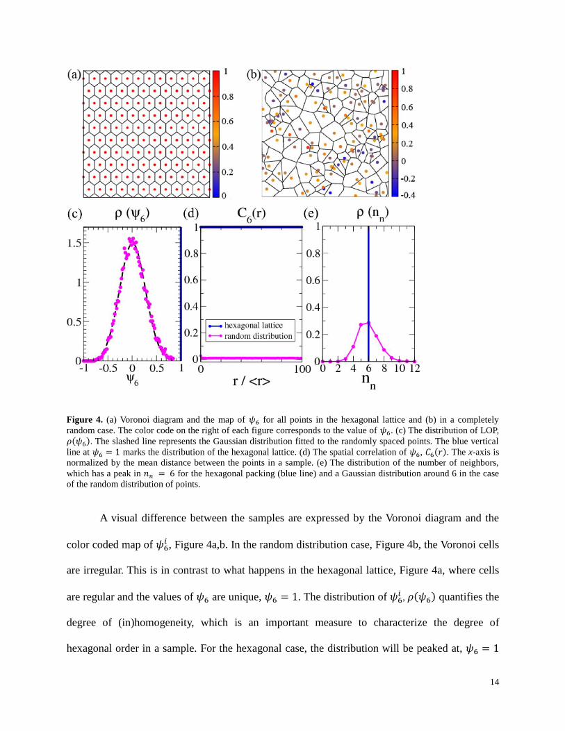
Figure 4. (a) Voronoi diagram and the map of 𝜓6 for all points in the hexagonal lattice and (b) in a completely

random case. The color code on the right of each figure corresponds to the value of 𝜓6. (c) The distribution of LOP,

𝜌(𝜓6). The slashed line represents the Gaussian distribution fitted to the randomly spaced points. The blue vertical

line at 𝜓6 = 1 marks the distribution of the hexagonal lattice. (d) The spatial correlation of 𝜓6, 𝐶6(𝑟). The x-axis is

normalized by the mean distance between the points in a sample. (e) The distribution of the number of neighbors,

which has a peak in 𝑛𝑛 = 6 for the hexagonal packing (blue line) and a Gaussian distribution around 6 in the case

of the random distribution of points.

A visual difference between the samples are expressed by the Voronoi diagram and the

color coded map of 𝜓6𝑖 , Figure 4a,b. In the random distribution case, Figure 4b, the Voronoi cells

are irregular. This is in contrast to what happens in the hexagonal lattice, Figure 4a, where cells

are regular and the values of 𝜓6 are unique, 𝜓6 = 1. The distribution of 𝜓6𝑖

, 𝜌(𝜓6) quantifies the

degree of (in)homogeneity, which is an important measure to characterize the degree of

hexagonal order in a sample. For the hexagonal case, the distribution will be peaked at, 𝜓6 = 1

15

while the random case displays a Gaussian distribution with an average given by ⟨𝜓6⟩ = 0, as

shown in Figure 4c.

To go beyond this local analysis of the order, we compute the spatial correlation of the

𝜓6, C6. The quantity C6 is a measure of how far the local order parameter is correlated in space.

The correlation functions for the two examples considered are shown in Figure 4d. For the

perfect hexagonal lattice, where all sites have 𝜓6𝑖 = 1 , it does not matter how far two points i

and j are, the correlation between the LOP of both sites will be 1. However, if points are

randomly distributed, C6 decays to zero very fast, indicating that even very close neighbors

points have their LOP uncorrelated. At large distances, when the sites are not correlated

anymore, the asymptotic value of C6 is ⟨𝜓6⟩2.

The most valuable information that can be extracted from C6 is the way it decays, i.e. its

functional dependence. When C6 decays exponentially, this decay is related to the typical sizes of

the regions where 𝜓6 have the same value. This is related with the typical grain size of a sample.

A third quantity that can be extracted from this analysis is the distribution of neighbors,

shown in Figure 4e. For a perfect hexagonal lattice, each point has exactly 6 neighbors, while in

any other case the number of neighbors is distributed around this value: the deviation from this

value increases with the disorder. In a hexagonally ordered array, points with 5 or 7 neighbors are

related to topological defects of the lattice. Depending on the neighborhood they can form

dislocations or disclinations, and their presence characterize hexatic or disordered structures,

with specific form for the decay of orientational correlations.

As described in section SECTION KTHNY, there are two kinds of order to completely

characterize hexagonal phase in a real solid,29

the positional order and the orientational order. In

our samples the orientational correlations decay at best as a power law of the distance from a

16

particular site. In this case it is expected that positional correlations, which are more sensitive to

defects, decay faster, typically exponentially fast. We have indeed verified this computing the

RDF for our samples. Then, this quantity would not discriminate between different levels of

order in the samples and for this reason we did not include an analysis of RDF in our work.

Quantification of the hexagonal order in a NAA: results and discussion (section

YYYYY)

In this section we apply the quantities explained in the previous section for the 2 extreme

cases in the samples of NAA. Before computing the LOP and its spatial correlations, it was

necessary to obtain the coordinates of the nanopores center. To do so, we adjust ellipses for each

nanopore totalizing 1245 nanopores for S1, 484 for S2 and 977 nanopores for S4. This allows the

definition of the center of mass of each nanopore, and the values of the major and minor semi

axes of the ellipses are related to the size of the pores. It was done with a standard software

package, in our case we used ImageJ.32

The center of the nanopores and other measures like the

distribution of nanopores diameter can be obtained with this software.

Three different samples of NAA structure were prepared by anodization process. The

process was carried out in two anodization steps, in a conventional 2 electrode cell using a Cu

sheet as a cathode. The anode is made of Al with two different degrees of purity, i.e., high purity

Al Bulk (99.999 %) and commercial Al (99.5 %). After each anodization step the samples were

dipped in a 5 wt% H3PO4 solution at 35 ± 1 °C for different times to remove the alumina formed

in the first anodization step. A second anodization step was performed to allow the opening of

nanopores. Table 1 summarizes the anodization conditions and the name that will be used for

each sample. After the anodization process the morphological nanoporous structure was

17

characterized by Scanning Electron Microscopy (SEM, JEOL JSM 6060) operating at 20 kV

acceleration voltages.

Figure 5a-c shows the SEM images of the S1, S2 and S3 samples, respectively, prepared

with different Al characteristics and anodization parameters, as described in the Table 1. The

anodization of the S1, S2 and S3 yielded NAA with different average diameters, as it can be

verified in the Table 1, leading to different visual levels in nanopores order. The Voronoi diagram

and the map of 𝜓6 are visual tools to identify the degree of order of the different anodization

systems, as shown in Figure 5d-f. It shows much more red points (corresponding to 𝜓6 = 1 in

the color code) and that they are concentrated in regions where the Voronoi cells are hexagonal.

Moreover, it is possible to observe that the hexagonal order is decreasing from S1 to S3 samples,

and for the last ones there are very few red points. Then this visual inspection clearly indicates

that S1 and S2 samples have higher ordering level of NAA, compared with S3. This result is due

to the higher purity of the Al matrix in S1 and S2 samples, while the S3 sample presents more

impurities, which hampers the formation of NAA with hexagonal order.

18

Figure 5. SEM images of the experimental samples of alumina nanopores, where (a) S1, (b) S2 and (c) S3. The

figures (d), (e), (f) represent the quantitative map of the 𝜓6 and the Voronoi diagram for the respective samples. The

colors indicate the value of 𝜓6 for each nanopore. The colour code is below each figure.

Table 1. Anodization conditions used for the 3 different alumina nanoporous samples.

sample

name material

anodization steps

1st 2

nd

condition Etching (min) condition Etching (min)

S1 Al (99.999%) a 50 a 10

S2 Al (99.999%) b 90 b 30

S3 Al (99.5%) a 30 a 10

a 0.3 M H2SO4, 25 V at 3±2 °C for 12 h;

b 0.3 M H2C2O4, 30 V at 15±2 °C for 12 h;

Figure 6a-c summarizes the quantitative analysis of nanopores ordering with the

distribution of the local order parameter 𝜓6, correlations C6 and the distribution of the number of

19

neighbors 𝜌(𝑛𝑛), respectively. For sample S1, has ⟨𝜓6⟩ ≈ 0.79 and the distribution is

completely asymmetric, indicating that most of nanopores form hexagons with their neighbors.

Sample S2 is also asymmetric and has most of the nanopores with a large value of 𝜓6, which

results in a relatively large average, ⟨𝜓6⟩ = 0.56, but the standard deviation, 𝜎 = 0.34, that

indicates more disorder than in sample S1. The S3 sample shows a more symmetric distribution

around ⟨𝜓6⟩ = 0.27. This indicates that the sample is much more disordered than the previous

cases (S1 and S2 samples), but it still has around 27 % more order than the completely random

case, for which ⟨𝜓6⟩ = 0. The dashed Gaussian curve drawings in Figure 6a-c represents the

distribution for a random set of points discussed in the section 2 and is a benchmark of such

completely disordered case.

In the middle column of Figure 6a-c, C6 indicates how far 𝜓6 is correlated in space. The

x-axis is normalized by the mean distance between the nanopores. We note that in the sample S1

the correlation decays very slowly: after 20 nanopores (which corresponds to more than half of

the system size in this case) and, the correlation is about 60 % of the nearest neighbor value. For

sample S2, although the absolute value of the correlation is smaller than in S1 case, the decay of

C6 is also slow, while for sample S3 the decay is very fast. In the case of S3, after a distance

equivalent to 2 average distance between nanopores, the correlation is so small that one can

conclude that the LOP of nanopores are not correlated anymore. This suggests that the grain size

is comparable to the size of a pore.9

The distribution of neighbors shows that the dispersion around the value 𝑛𝑛 = 6

increases from S1 to S3, also pointing to an increase of the disorder and indicating that there are

more topological defects in S3 than in S1.

20

Figure 6. First column: distribution of 𝜓6, 𝜌(𝜓6). Second column: correlation of 𝜓6, 𝐶6. Third column: distribution

of the number of neighbors, 𝜌(𝑛𝑛). In each line we show all the quantities for different samples, from (a) to (c), in

the same order as in Figure 3. In all figures we plot dashed curves that represent the random distribution of points

discussed in Section 2 and are used here to be compared with the samples of NAA.

Interpretation of the results in terms of the KTHNY theory

One can rationalize the results obtained for these samples in the light of the theory of

two-dimensional melting, or KTHNY theory.29, 30

The most ordered sample analyzed here, S1, is

not a perfectly ordered sample. The presence of defects is evident from the distributions 𝜌(𝜓6)

and 𝜌(𝑛𝑛). Since the correlations of the order parameter decay slowly, the behavior is analogous

to the hexatic phase. Sample S2 has also a behavior of its correlation function analogous to a

hexatic phase although it has more defects than the sample S2. The picture changes for sample

21

S3. In this case, the system has still more defects and they are enough to destroy completely the

correlation of 𝜓6. As can be seen in Figure 6c, C6 decays very fast, typically exponentially with

the distance from any point in space. If a fit to an exponential decay, 𝐶6~𝑒(−𝑟/𝑥𝑖), would be

possible, xi might be interpreted as a typical grain size of the sample, which is too small in this

case, being only about 2-3 interpore distances. This result can be interpreted as a result of the

impurities present in the Al matrix.

Conclusions

In this chapter we discussed some methods to quantify the hexagonal order in NAA. In

the first part of the chapter we presented some methods found in the literature. We first discussed

the Fourier Transform and correlation functions of position and angles and pointed out that these

are very qualitative methods. They do not return a number to quantify order and are not able to

discriminate quantitatively between cases where the samples have defects. We then presented

more quantitative methods, where the idea is to quantify the difference between a given network

of points and a hexagonal lattice. Hillebrand et al24

and Matefi et al26

proposed useful methods

that allow for a determination of the grain size, although they rely on a threshold parameter. We

also discussed briefly a recent approach based on an analysis of the intensity of the signal of a

given image, which can be useful to identify the directions of different domains, but not to

quantify order of the whole sample.23

In the second part, we proposed a new method to quantitatively characterize hexagonal

arrays of NAA. The approach presented is inspired in a statistical mechanical theory developed

to describe phase ordering in two dimensional systems. For each nanopore, its neighbors are

defined using Voronoi tessellation and then a local order parameter (LOP) called the hexatic

22

order parameter is defined, 𝜓6, to quantify how close a given nanopore is from a perfect

hexagon. The correlation of this parameter at two different points of the array, C6, informs how

long the local orientational order spreads in the sample.

We first presented the method for a hypothetical network of points and computed the

defined quantities for two extreme cases, a perfectly hexagonal network and a completely

random distribution of points. Then, the developed tools were applied to the NAA. We showed

that the average value of 𝜓6 quantifies the degree of orientational order in a sample and its

standard deviation is a measure of how heterogeneous is this local order. The correlation of this

hexatic order parameter characterizes the range of the local order and allows a determination of

the size of highly ordered domains in the sample.

We emphasize that this method can be easily extended to characterize any kind of system

that presents hexagonal networks. If the experimental images can be treated to define the center

of mass of the pores, the method is quite general, easy to implement and has no arbitrary

parameters. We expect that this way of characterizing order in NAA and the analogy with other

physical systems showing hexagonal packing arrays will help to improve the theoretical

modeling to better understand how long range order in the NAA and similar systems develop,

and from which better suited experiments can be proposed and devised.

Acknowledgment

This work was partially sponsored by CNPq (no. 471220/2010-8), FAPERGS (n

o.

11/2000-4), CAPES (Brazilian funding agencies). Thanks also to the “Centro de Microscopia

Eletronica (CME) of the Universidade Federal do Rio Grande do Sul.”

23

References

1. Lee, W., JOM 2010, 62 (6), 57-63.

2. Jessensky, O.; Muller, F.; Gosele, U., Appl. Phys. Lett. 1998, 72 (10), 1173-1175.

3. Li, A. P.; Muller, F.; Birner, A.; Nielsch, K.; Gosele, U., J. Appl. Phys. 1998, 84 (11),

6023-6026.

4. Li, F. Y.; Zhang, L.; Metzger, R. M., Chem. Mater. 1998, 10 (9), 2470-2480.

5. Lee, W.; Ji, R.; Gosele, U.; Nielsch, K., Nat. Mater. 2006, 5 (9), 741-747.

6. Chu, S. Z.; Wada, K.; Inoue, S.; Isogai, M.; Yasumori, A., Adv. Mater. 2005, 17 (17),

2115-2119.

7. Nielsch, K.; Choi, J.; Schwirn, K.; Wehrspohn, R. B.; Gosele, U., Nano Lett. 2002, 2 (7),

677-680.

8. Feil, A. F. Nanoestruturas de óxidos de Al e Ti obtidas a partir do processo de anodização:

fabricação, caracterização e aplicações. Tese de Doutorado, Universidade Federal do Rio Grande

do Sul - UFRGS, Porto Alegre, 2009.

9. Feil, A. F.; da Costa, M. V.; Amaral, L.; Teixeira, S. R.; Migowski, P.; Dupont, J.;

Machado, G.; Peripolli, S. B., J. Appl. Phys. 2010, 107 (2), 026103.

10. Weibel, D. E.; Michels, A. F.; Feil, A. F.; Amaral, L.; Teixeira, S. R.; Horowitz, F., J.

Phys. Chem. C 2010, 114 (31), 13219-13225.

11. Feil, A. F.; da Costa, M. V.; Migowski, P.; Dupont, J.; Teixeira, S. R.; Amaral, L., J.

Nanosci. Nanotechnol. 2011, 11 (3), 2330-2335.

12. Feil, A. F.; Migowski, P.; Dupont, J.; Amaral, L.; Teixeira, S. R., J. Phys. Chem. C 2011,

115 (15), 7621-7627.

13. Baik, J. M.; Schierhorn, M.; Moskovits, M., J. Phys. Chem. C 2008, 112 (7), 2252-2255.

14. Gadot, F.; Chelnokov, A.; DeLustrac, A.; Crozat, P.; Lourtioz, J. M.; Cassagne, D.;

Jouanin, C., Appl. Phys. Lett. 1997, 71 (13), 1780-1782.

15. Wang, Y. D.; Zang, K. Y.; Chua, S. J.; Sander, M. S.; Tripathy, S.; Fonstad, C. G., J. Phys.

Chem. B 2006, 110 (23), 11081-11087.

16. Lee, W.; Jin, M. K.; Yoo, W. C.; Lee, J. K., Langmuir 2004, 20 (18), 7665-7669.

17. Feil, A. F.; Weibel, D. E.; Corsetti, R. R.; Pierozan, M. D.; Michels, A. F.; Horowitz, F.;

Amaral, L.; Teixeira, S. R., ACS Appl. Mater. Interfaces 2011, 3 (10), 3981-3987.

18. Borba, J. R.; Brito, C.; Migowski, P.; Vale, T. B.; Stariolo, D. A.; Teixeira, S. R.; Feil, A.

F., J. Phys. Chem. C 2012, ASAP.

19. Brito, C. http://www.lief.if.ufrgs.br/~cbrito/nanoporos/.

20. Napolskii, K. S.; Roslyakov, I. V.; Eliseev, A. A.; Petukhov, A. V.; Byelov, D. V.;

Grigoryeva, N. A.; Bouwman, W. G.; Lukashin, A. V.; Kvashnina, K. O.; Chumakov, A. P.;

Grigoriev, S. V., J. Appl. Crystallogr. 2010, 43, 531-538.

21. Napolskii, K. S.; Roslyakov, I. V.; Eliseev, A. A.; Byelov, D. V.; Petukhov, A. V.;

Grigoryeva, N. A.; Bouwman, W. G.; Lukashin, A. V.; Chumakov, A. P.; Grigoriev, S. V., J. Phys.

Chem. C 2011, 115 (48), 23726-23731.

22. Leitao, D. C.; Apolinario, A.; Sousa, C. T.; Ventura, J.; Sousa, J. B.; Vazquez, M.; Araujo,

J. P., J. Phys. Chem. C 2011, 115 (17), 8567-8572.

23. Kashi, M. A.; Ramazani, A., J. Phys. D-Appl. Phys. 2005, 38 (14), 2396-2399.

24. Hillebrand, R.; Muller, F.; Schwirn, K.; Lee, W.; Steinhart, M., Acs Nano 2008, 2 (5),

24

913-920.

25. Pichler, S.; Bodnarchuk, M. I.; Kovalenko, M. V.; Yarema, M.; Springholz, G.; Talapin,

D. V.; Heiss, W., Acs Nano 2011, 5 (3), 1703-1712.

26. Matefi-Tempfli, S.; Matefi-Tempfli, M.; Piraux, L., Thin Solid Films 2008, 516 (12),

3735-3740.

27. Abdollahifard, M. J.; Faez, K.; Pourfard, M.; Abdollahi, M., Appl. Surf. Sci. 2011, 257

(24), 10443-10450.

28. Pourfard, M.; Faez, K., Appl. Surf. Sci. 2012, 259 (0), 124-134.

29. Nelson, D. R., Defects and Geometry in Condensed Matter Physics. Cambridge

University Press, Cambridge: 2002.

30. Gasser, U.; Eisenmann, C.; Maret, G.; Keim, P., ChemPhysChem 2010, 11 (5), 963-970.

31. Atsuyuki, O.; Barry, B.; Kokichi, S., Spatial tessellations: concepts and applications of

Voronoi diagrams. John Wiley \\& Sons, Inc.: 1992; p 532.

32. ImageJ, public domain. http://rsbweb.nih.gov/ij/.