quantitative and qualitative analyses of requirements elaboration
156
QUANTITATIVE AND QUALITATIVE ANALYSES OF REQUIREMENTS ELABORATION FOR EARLY SOFTWARE SIZE ESTIMATION by Ali Afzal Malik A Dissertation Presented to the FACULTY OF THE USC GRADUATE SCHOOL UNIVERSITY OF SOUTHERN CALIFORNIA In Partial Fulfillment of the Requirements for the Degree DOCTOR OF PHILOSOPHY (COMPUTER SCIENCE) August 2010 Copyright 2010 Ali Afzal Malik
Transcript of quantitative and qualitative analyses of requirements elaboration
QUANTITATIVE AND QUALITATIVE ANALYSES
OF REQUIREMENTS ELABORATION
FOR EARLY SOFTWARE SIZE ESTIMATION
by
Ali Afzal Malik
A Dissertation Presented to the FACULTY OF THE USC GRADUATE SCHOOL UNIVERSITY OF SOUTHERN CALIFORNIA
In Partial Fulfillment of the Requirements for the Degree DOCTOR OF PHILOSOPHY
(COMPUTER SCIENCE)
August 2010
Copyright 2010 Ali Afzal Malik

ii
Dedication
I dedicate this work to the One and Only Who has the most beautiful names.

iii
Acknowledgements
First and foremost, I thank the Almighty for giving me the ability to pursue
this research. Whatever good I possess is from Him alone. His blessings are
uncountable and priceless. Good health, caring family members, knowledgeable
mentors, cooperative colleagues, and generous sponsors are just a few of these
blessings.
My family’s love, care, and support has played a vital role in reaching thus
far. My late father taught me the value of education and instilled in me the desire to
strive for the best. My mother’s encouragement and moral support helped me to
overcome various obstacles in life. My elder brother took the lion’s share of
household responsibilities after my father passed away. This allowed me to give
undivided attention to my studies. My wife’s emotional and spiritual support has
provided the much-needed motivation to take this research to fruition.
I owe a lot to my research advisor and dissertation committee chair – Dr
Barry Boehm. His remarkable knowledge, vast experience, and good nature make
him one of the best mentors. Dr. Boehm’s expert advice and constructive criticism
have been invaluable in tackling this hard research problem. I am also indebted to
other members of my qualifying exam and dissertation committees i.e. Dr. Nenad
Medvidović, Dr. Bert Steece, Dr. Rick Selby, and Dr. Ellis Horowitz. Each of these
individuals has played an important role in refining this research.
A number of my colleagues have been instrumental in conducting this
research. Supannika Koolmanojwong, Pongtip Aroonvatanaporn, Dr. Ye Yang

iv
(ISCAS) and Yan Ku (ISCAS) have provided invaluable assistance in data
collection. Julie Sanchez (CSSE Administrator) and Alfred Brown (CSSE System
Administrator) have provided valuable support in a number of vital administrative
and technical maters.
Last, but certainly not the least, I thank my sponsors – Fulbright, HEC
Pakistan, and USAID – for giving me an opportunity to pursue graduate studies i.e.
MS and PhD degrees. Their comprehensive financial assistance has enabled me to
study at one of the most prestigious universities in the world i.e. USC.

v
Table of Contents
Dedication ........................................................................................................................... ii Acknowledgements............................................................................................................ iii List of Tables .................................................................................................................... vii List of Figures .................................................................................................................... ix Abbreviations................................................................................................................... xiii Abstract ............................................................................................................................. xv Chapter 1 Introduction ........................................................................................................ 1
1.1 Problem Definition.................................................................................................... 1 1.2 Research Approach ................................................................................................... 3 1.3 Research Significance............................................................................................... 4 1.4 Dissertation Outline .................................................................................................. 5
Chapter 2 Related Work...................................................................................................... 7
2.1 Sizing Methods ......................................................................................................... 7 2.2 Sizing Metrics ........................................................................................................... 9 2.3 Requirements Elaboration....................................................................................... 13
Chapter 3 From Cloud to Kite .......................................................................................... 18
3.1 Experimental Setting............................................................................................... 19 3.2 Method .................................................................................................................... 23 3.3 Results..................................................................................................................... 33 3.4 Elaboration of Capability Goals.............................................................................. 38 3.5 Utility of Elaboration Groups ................................................................................. 40 3.6 Threats to Validity .................................................................................................. 43
Chapter 4 From Cloud to Clam......................................................................................... 45
4.1 Experimental Setting............................................................................................... 46 4.2 Method .................................................................................................................... 47 4.3 Results and Discussion ........................................................................................... 51 4.4 Requirements Elaboration of Commercial Projects................................................ 56
Chapter 5 Efficacy of COCOMO II Cost Drivers in Predicting Elaboration Profiles...... 59
5.1 Method .................................................................................................................... 60 5.2 Results..................................................................................................................... 62 5.3 Discussion............................................................................................................... 75

vi
Chapter 6 Comparative Analysis of Requirements Elaboration ....................................... 78 6.1 Empirical Setting .................................................................................................... 78 6.2 Data Collection ....................................................................................................... 79 6.3 Results..................................................................................................................... 83 6.4 Comparison with Second Empirical Study............................................................. 87 6.5 Conclusions............................................................................................................. 89
Chapter 7 Determinants of Elaboration ............................................................................ 91
7.1 Stage 1 Cloud to Kite.............................................................................................. 91 7.2 Stage 2 Kite to Sea.................................................................................................. 94 7.3 Stage 3 Sea to Fish.................................................................................................. 95 7.4 Stage 4 Fish to Clam............................................................................................... 96
Chapter 8 Contributions and Next Steps........................................................................... 98
8.1 Main Contributions ................................................................................................. 98 8.2 Future Work.......................................................................................................... 100
Bibliography ................................................................................................................... 103 Appendix A Specification and Normalization of High-Level Requirements................. 108
A.1 Category vs. Instance ........................................................................................... 108 A.2 Aggregate vs. Component.................................................................................... 110 A.3 One-to-One........................................................................................................... 111 A.4 Main Concept and Related Minor Concept.......................................................... 112
Appendix B Multiple Regression Results for Small E-Services Projects....................... 115
B.1 First Stage of Elaboration..................................................................................... 115 B.2 Second Stage of Elaboration ................................................................................ 116 B.3 Third Stage of Elaboration ................................................................................... 116 B.4 Fourth Stage of Elaboration ................................................................................. 117
Appendix C COCOMO II Cost Drivers and Elaboration Profiles of SoftPM Versions. 118
C.1 COCOMO II Cost Driver Ratings........................................................................ 118 C.2 Results of Simple Regression Analyses ............................................................... 120

vii
List of Tables
Table 1: Projects used for first empirical study 21
Table 2: Metrics 29
Table 3: Values of metrics for capability goals and capability requirements 33
Table 4: Values of metrics for LOS goals and LOS requirements 34
Table 5: Elaboration determinants 42
Table 6: Projects used for second empirical study 47
Table 7: Mapping 48
Table 8: Relevant artifacts 49
Table 9: Formulae for elaboration factors 51
Table 10: Elaboration factor sets for each project 52
Table 11: Summary of elaboration results 54
Table 12: Multi-level requirements data of large IBM projects 57
Table 13: Elaboration factors of large IBM projects 57
Table 14: Cost driver rating scale 60
Table 15: COCOMO II scale factor ratings 63
Table 16: COCOMO II product factor ratings 64
Table 17: COCOMO II platform factor ratings 65
Table 18: COCOMO II personnel factor ratings 66
Table 19: COCOMO II project factor ratings 67
Table 20: Correlation between CG
CR
and COCOMO II cost drivers 69

viii
Table 21: Correlation between CR
UC
and COCOMO II cost drivers 70
Table 22: Correlation between UC
UCS
and COCOMO II cost drivers 71
Table 23: Correlation between UCS
SLOC
and COCOMO II cost drivers 72
Table 24: COCOMO II cost drivers relevant at each elaboration stage 74
Table 25: Results of multiple regression analysis 75
Table 26: Requirements levels of SoftPM 79
Table 27: Multi-level requirements data of SoftPM 83
Table 28: Elaboration profiles 84
Table 29: Summary statistics of elaboration factors 86
Table 30: Comparison of summary statistics 88
Table 31: Determinants of elaboration 99
Table 32: Scale factor ratings 118
Table 33: Product factor ratings 119
Table 34: Platform factor ratings 119
Table 35: Personnel factor ratings 119
Table 36: Project factor ratings 119

ix
List of Figures
Figure 1: Cone of uncertainty 2
Figure 2: Sizing metrics 9
Figure 3: Cockburn’s metaphor illustrating refinement of use cases 14
Figure 4: SLOC/Requirement ratios of large-scale projects 16
Figure 5: Multiple requirements levels for large IBM projects 17
Figure 6: Partial software development process 22
Figure 7: Typical high-level capability goal with its low-level capability requirements 25
Figure 8: Typical high-level LOS goal with its low-level LOS requirement 26
Figure 9: Table of contents of OCD 27
Figure 10: Table of contents of SSRD 28
Figure 11: EF ranges defining different elaboration groups 31
Figure 12: Elaboration of capability goals into capability requirements 36
Figure 13: Elaboration of LOS goals into LOS requirements 37
Figure 14: Elaboration groups for capability goals 39
Figure 15: Data collection process 47
Figure 16: CG
CR
distribution 52
Figure 17: CR
UC
distribution 53
Figure 18: UC
UCS
distribution 53

x
Figure 19: UCS
SLOC
distribution 54
Figure 20: Elaboration of use cases to use case steps 55
Figure 21: Example scenario depicting overlaps amongst versions 80
Figure 22: Example scenario after removing overlaps amongst versions 81
Figure 23: Distribution of CG to CR elaboration factor 85
Figure 24: Distribution of CR to UC elaboration factor 85
Figure 25: Distribution of UC to UCS elaboration factor 85
Figure 26: Distribution of UCS to SLOC elaboration factor 86
Figure 27: Proportion of atomic capability goals 94
Figure 28: Proportion of atomic capability requirements 95
Figure 29: Proportion of alternative use case steps to main use case steps 96
Figure 30: EF(CG, CR) vs. PREC 121
Figure 31: EF(CG, CR) vs. FLEX 121
Figure 32: EF(CG, CR) vs. RESL 122
Figure 33: EF(CG, CR) vs. TEAM 122
Figure 34: EF(CG, CR) vs. PMAT 123
Figure 35: EF(CG, CR) vs. TIME 123
Figure 36: EF(CG, CR) vs. ACAP 124
Figure 37: EF(CG, CR) vs. PCAP 124
Figure 38: EF(CG, CR) vs. PCON 125
Figure 39: EF(CG, CR) vs. APEX 125
Figure 40: EF (CR, UC) vs. PREC 126

xi
Figure 41: EF (CR, UC) vs. FLEX 126
Figure 42: EF (CR, UC) vs. RESL 127
Figure 43: EF (CR, UC) vs. TEAM 127
Figure 44: EF (CR, UC) vs. PMAT 128
Figure 45: EF (CR, UC) vs. TIME 128
Figure 46: EF (CR, UC) vs. ACAP 129
Figure 47: EF (CR, UC) vs. PCAP 129
Figure 48: EF (CR, UC) vs. PCON 130
Figure 49: EF (CR, UC) vs. APEX 130
Figure 50: EF(UC, UCS) vs. PREC 131
Figure 51: EF(UC, UCS) vs. FLEX 131
Figure 52: EF(UC, UCS) vs. RESL 132
Figure 53: EF(UC, UCS) vs. TEAM 132
Figure 54: EF(UC, UCS) vs. PMAT 133
Figure 55: EF(UC, UCS) vs. TIME 133
Figure 56: EF(UC, UCS) vs. ACAP 134
Figure 57: EF(UC, UCS) vs. PCAP 134
Figure 58: EF(UC, UCS) vs. PCON 135
Figure 59: EF(UC, UCS) vs. APEX 135
Figure 60: EF(UCS, SLOC) vs. PREC 136
Figure 61: EF(UCS, SLOC) vs. FLEX 136
Figure 62: EF(UCS, SLOC) vs. RESL 137
Figure 63: EF(UCS, SLOC) vs. TEAM 137

xii
Figure 64: EF(UCS, SLOC) vs. PMAT 138
Figure 65: EF(UCS, SLOC) vs. TIME 138
Figure 66: EF(UCS, SLOC) vs. ACAP 139
Figure 67: EF(UCS, SLOC) vs. PCAP 139
Figure 68: EF(UCS, SLOC) vs. PCON 140
Figure 69: EF(UCS, SLOC) vs. APEX 140

xiii
Abbreviations
AEF Abnormal Elaboration Factor
CG Capability Goal
CMMI Capability Maturity Model Integration
COCOMO II Constructive Cost Model Version II
COSYSMO Constructive Systems Engineering Cost Model
COTS Commercial of-the-Shelf
CR Capability Requirement
CSSE Center for Systems and Software Engineering
EF Elaboration Factor
EP Elaboration Profile
HEF High Elaboration Factor
ICM-Sw Incremental Commitment Model for Software
IOC Initial Operational Capability
IV & V Independent Verification and Validation
KSLOC Thousand Source Lines of Code
LCO Life Cycle Objectives
LCP Life Cycle Plan
LEF Low Elaboration Factor
LOS Level of Service
MBASE Model-Based (System) Architecting and Software Engineering
MEF Medium Elaboration Factor
xiv
OCD Operational Concept Description
RL Requirements Level
RUP Rational Unified Process
SAIV Schedule as Independent Variable
SE Software Engineering
SLOC Source Lines of Code
SSAD System and Software Architecture Description
SSRD System and Software Requirements Definition
UC Use Case
UCS Use Case Step
UML Unified Modeling Language
USC University of Southern California

xv
Abstract
Software size is one of the most influential inputs of a software cost estimation
model. Improving the accuracy of size estimates is, therefore, instrumental in improving
the accuracy of cost estimates. Moreover, software size and cost estimates have the
highest utility at the time of inception. This is the time when most important decisions e.g.
budget allocation, personnel allocation, etc. are taken. The dilemma, however, is that only
high-level requirements for a project are available at this stage. Leveraging this high-
level information to produce an accurate estimate of software size is an extremely
challenging task.
Requirements for a software project are expressed at multiple levels of detail
during its life cycle. At inception, requirements are expressed as high-level goals. With
the passage of time, goals are refined into shall statements and shall statements into use
cases. This process of progressive refinement of a project’s requirements, referred to as
requirements elaboration, continues till source code is obtained. This research analyzes
the quantitative and qualitative aspects of requirements elaboration to address the
challenge of early size estimation.
A series of four empirical studies is conducted to obtain a better understanding of
requirements elaboration. The first one lays the foundation for the quantitative
measurement of this abstract process by defining the appropriate metrics. It, however,
focuses on only the first stage of elaboration. The second study builds on the foundation
laid by the first. It examines the entire process of requirements elaboration looking at
each stage of elaboration individually. A general process for collecting and processing

xvi
multi-level requirements to obtain elaboration data useful for early size estimation is
described. Application of this general process to estimate the size of a new project is also
illustrated.
The third and fourth empirical studies are designed to tease out the factors
determining the variation in each stage of elaboration. The third study focuses on
analyzing the efficacy of COCOMO II cost drivers in predicting these variations. The
fourth study performs a comparative analysis of the elaboration data from two different
sources i.e. small real-client e-services projects and multiple versions of an industrial
process management tool.

1
Chapter 1 Introduction
1.1 Problem Definition
Software cost models are best described as “garbage in-garbage out devices”
[Boehm, 1981]. The quality of the outputs of these models is determined by the quality of
the inputs. Hence, if input quality is bad, output quality cannot be good. This fact clearly
implies that one of the prerequisites of improving the estimates (outputs) of these models
is to improve the quality of the inputs supplied to these models.
Different parametric cost models such as SLIM [Putnam, 1978], PRICE-S
[Freiman and Park, 1979], COCOMO II [Boehm et al., 2000], and COSYSMO [Valerdi,
2005] require a different set of inputs. One input, however, is common amongst most of
these models i.e. “an estimate of likely product size” [Fenton and Pfleeger, 1997]. In fact,
size is the most influential input of these models. The accuracy of cost estimation
“depends more on accurate size estimates than on any other cost-related parameter”
[Pfleeger, Wu, and Lewis, 2005].
The fundamental challenge of cost estimation, therefore, is “estimating the
amount (size) of software that must be produced” [Stutzke, 2005]. Addressing this
challenge lies at the crux of improving cost estimation accuracy. Producing an accurate
estimate of product size, however, is not an easy task.
The difficulty of accurate size estimation is compounded especially at the time of
inception when very little information is available. This problem is visually depicted in
the “cone of uncertainty” diagram from [Boehm et al., 2004] which is reproduced in
Figure 1. This diagram plots the relative size range versus the various phases and

2
milestones. It clearly indicates that, at the beginning of a project, estimates are far off
from the actual values. As time progresses, the error in estimation starts decreasing but so
does the utility of these estimates.
Figure 1: Cone of uncertainty
The cone of uncertainty highlights the fundamental dilemma of system and
software size estimation i.e. the tradeoff between accuracy and utility of estimates.
Estimates are of highest value at the beginning of a project. This is the time when
important decisions such as those regarding budget and personnel allocation are made.
Estimation accuracy at this point, however, is lowest. Therefore, in order to achieve
maximum utility, it is extremely important to improve the accuracy of estimates produced
at the time of inception.

3
Improving the accuracy of early size estimation necessitates leveraging high-level
project requirements available at the time of inception i.e. project goals and objectives.
Leveraging this information about the high-level requirements of a project is only
possible if one is aware of the details of the process of their elaboration into lower-level
requirements e.g. shall statements, use cases, etc. These details about the process of
elaboration are previously unavailable. This problem is succinctly summarized in the
following statement:
At the time of a project’s inception, when estimates have the highest utility, very high-level requirements are available and the elaboration process of these high-level requirements is unknown.
1.2 Research Approach
Requirements for any project can be expressed at multiple levels of detail e.g.
goals (least detailed), shall statements, use cases, use case steps, and SLOC (most
detailed). At the time of a project’s inception, requirements are usually expressed as high-
level goals. With the passage of time, these goals are elaborated into shall statements,
shall statements are transformed into use cases, use cases are decomposed into use case
steps, and use case steps are implemented by SLOC. Each subsequent level builds on the
previous by adding more detail. This progressive refinement of requirements is called
requirements elaboration. This research addresses the problem identified in the previous
section by uncovering the details of this process of requirements elaboration.
The mechanics of this abstract process of requirements elaboration are studied by
first measuring this process quantitatively using metrics specifically designed for this

4
purpose. The quantification of this process, in turn, facilitates looking at its qualitative
nuances. It helps in teasing out factors that determine its variations.
1.3 Research Significance
A deeper understanding of the quantitative and qualitative aspects of the
requirements elaboration process provides a number of benefits. First and foremost, it
helps in solving the fundamental dilemma of system and software size estimation i.e.
estimates are less accurate when their utility is more and more accurate when their utility
is less. Leveraging a project’s high-level requirements by studying the elaboration
process enables producing accurate estimates when estimation accuracy really matters i.e.
at the time of inception.
Another important benefit of this work is that quantitative information about
requirements elaboration helps in resolving inconsistencies between the level of detail of
model inputs and model calibration data. If not resolved, such inconsistencies can easily
lead to over- or under-estimation of cost. Consider, for instance, a model that has been
calibrated using lower-level requirements such as shall statements as one of the inputs.
Using higher-level requirements such as goals as an input to this model will result in an
under-estimation of cost. However, if the elaboration process of higher-level
requirements is known, these high-level goals can be converted to equivalent lower-level
shall statements expected as input by the model.
Last but not the least, quantitative measures of elaboration allow comparisons
between estimates of models that use different size parameters. As an example, consider
two cost estimation models A and B. If, for instance, model A uses shall statements as

5
input while model B uses SLOC, then the outputs of these two models can be made
comparable only after transforming the shall statements into equivalent SLOC and
plugging this value into model B. Transforming shall statements into equivalent SLOC,
however, requires understanding how shall statements elaborate into SLOC. The analyses
presented in this research help in achieving this understanding.
1.4 Dissertation Outline
The rest of this dissertation is organized as follows:
• Chapter 2 briefly describes previous work relevant to this research. It surveys
prior work in three areas i.e. software sizing, software metrics, and requirements
elaboration. Gaps and shortcomings in prior work are also highlighted in this
chapter.
• Chapter 3 describes the first empirical study on requirements elaboration. This
study analyzes the first stage of requirements elaboration. It examines the
elaboration of two different types of goals – capability and level of service (LOS)
– into respective immediately lower-level requirements. New metrics are
introduced to quantitatively measure requirements elaboration.
• Chapter 4 summarizes the second empirical study which examines the entire
process of requirements elaboration. A five-step process for gathering and
processing a project’s multi-level requirements to obtain its elaboration data is
described. The utility of summary statistics obtained from the elaboration data of
multiple similar projects in early size estimation is illustrated. A case study

6
showing the application of this approach in estimating the size of a large new
IBM project is also included.
• Chapter 5 presents the third empirical study which determines the efficacy of
COCOMO II cost drivers in predicting variations in different stages of
elaboration. For each stage of elaboration, the relationship between the values of
the relevant cost drivers and the magnitude of elaboration is analyzed.
• Chapter 6 describes the fourth and final empirical study on requirements
elaboration. This study first presents a novel approach to determine the
elaboration profiles of different versions of an industrial product. It then
compares these elaboration profiles with the elaboration profiles obtained in the
second empirical study.
• Chapter 7 contains a discussion on the determinants of elaboration. It presents the
factors responsible for variations in different stages of elaboration.
• Chapter 8 concludes this dissertation by summarizing the major contributions of
this research. It also highlights avenues for future work in this area.

7
Chapter 2 Related Work
2.1 Sizing Methods
A number of methods for estimating size have been proposed in the literature. A
good overview of these methods can be found in [Boehm, 1981], [Fenton and Pfleeger,
1997], and [Stutzke, 2005]. Most of these methods can be classified into four major
categories: expert judgment, analogy-based, group consensus, and decomposition.
As is evident from the name, size estimation based on expert judgment takes
advantage of the past experience of an expert. A seasoned developer is requested to
estimate the size of a project based on the information available about the project. One of
the main advantages of this approach is that experts can spot exceptional size drivers. The
accuracy of the estimate, however, is completely dependent on the experience and
memory of the expert.
Analogy-based size estimation methods use one or more benchmarks for
estimating the size of a new project. The characteristics of the new project are compared
with the benchmarks. The size of the new project is adjusted based on the similarities and
differences between the new project and the benchmarks. Pair-wise comparison is a
special case of analogy-based sizing which uses a single reference point. This type of
estimation can only be employed when suitable benchmarks are available. The main
advantage of this approach is that it uses relative sizing which prevents most of the
problems associated with absolute sizing such as personal bias and incomplete recall.
Group consensus techniques such as Wideband Delphi [Boehm, 1981] and
Planning Poker [Cohn, 2005] use a group of people instead of individuals to derive

8
estimates of size. Estimation activities are coordinated by a moderator who describes the
scenario, solicits estimates, and compiles the results. At the end of the first round,
divergences are discussed and individuals share rationales for their estimation values.
More rounds of estimation may be necessary to reach a consensus. The main advantage
of these techniques is that they improve understanding of the problem through group
discussion. Iteration and group coordination, however, requires more time and resources
than techniques relying on a single person.
Decomposition techniques for estimating size use a more rigorous approach. Two
complementary decomposition techniques are available: top-down and bottom-up. Top-
down estimation focuses on the product as a whole. Estimates of the overall size are
derived from the global product characteristics and are then assigned proportionally to
individual components of the product. Bottom-up estimation, on the other hand, focuses
on the individual components. Size is estimated for each individual component. The size
of the overall product is then derived by summing the size of the individual components.
Since these two techniques are orthogonal, the advantages of one are the disadvantages of
the other. The top-down approach has a system-level focus but lacks a detailed basis. The
bottom-up approach, on the other hand, has a more detailed basis but tends to ignore
overall product characteristics.
Apart from the four main size estimation method categories mentioned above,
other categories also exist. Probabilistic methods such as PERT sizing [Putnam and
Fitzsimmons, 1979] are an example. Fuzzy logic-based size estimation methods such as
those described in [Putnam and Myers, 1992] and [MacDonell, 2003] are another
example.

9
Combinations of sizing methods belonging to different categories are also
possible options. For instance, pair-wise comparisons may be used in conjunction with
top-down estimation to derive an estimate of size. Similarly, expert judgment may be
combined with bottom-up estimation.
The basic problem, which none of these methods addresses, is the high amount of
uncertainty involved in early size estimation. This uncertainty stems from the fact that
very little information is available at the time of inception. Thus, as shown in the cone of
uncertainty (see Figure 1), estimates produced at the time of inception are far off from the
actual values.
2.2 Sizing Metrics
Process Phase
Possible Measures
Primary Aids
Concept Elaboration Construction
Increasing Time and Detail
Subsystems Key Features
User Roles, Use Cases
Screens, Reports,
Files, Application
Points
Function Points Components Objects
Source Lines of Code, Logical
Statements
Product Vision,
Analogies
Operational Concept, Context Diagram
Specification, Feature List
Architecture, Top Level
Design
Detailed Design Code
Figure 2: Sizing metrics
Product size can be expressed using a number of different metrics. A vast
majority of the commonly used size metrics is captured by Figure 2 which is reproduced

10
from [Stutzke, 2005]. This figure shows the metrics available at different process phases
along with the primary aids which act as sources for deriving values for these metrics. In
the construction phase, for instance, size can be measured in terms of the number of
objects specified in the detailed design.
The possible measures listed in Figure 2 can be divided into two broad categories
i.e. functional size measures and physical size measures. Functional size refers to the size
of the software in terms of its functionality while physical size refers to the size of the
software in terms of the amount of code. Each of these measures has benefits and
shortcomings. Functional size measures are technology independent and can be obtained
earlier than physical size measures. However, it is difficult to automate the counting of
functional size. Physical size measures, on the other hand, are technology dependent but
can be obtained automatically.
Function Point Analysis [Albrecht, 1979] is the most popular functional size
measure. Many versions of Function Point Analysis are being used throughout the world.
In USA, the IFPUG version of function points [IFPUG, 2010] is the most popular
methodology. In a nutshell, IFPUG function points measure the functionality of a system
by identifying its components (i.e. inputs, outputs, data files, interfaces, and inquiries)
and rating each component according to its complexity (i.e. simple, average, and
complex). Once each component has been assigned its complexity rating, these ratings
are summed-up to obtain unadjusted function points. Unadjusted function points are
multiplied by a value adjustment factor calculated using overall application
characteristics to obtain the adjusted function points.

11
Other significantly-popular versions of Function Point Analysis (FPA) include
COSMIC Full Function Points [COSMIC, 2009], Mk II FPA [UKSMA, 1998], and
NESMA FPA [NESMA, 2004]. There are a number of conceptual and procedural
differences between IFPUG and COSMIC methods. For instance, unlike IFPUG function
points that use five functional component types, COSMIC Full Function Points use four
i.e. entry, read, write, and exit. Nonetheless, both IFPUG and COSMIC functional size
methods are international standards. Mk II FPA, used mainly in the United Kingdom,
employs only three component types i.e. inputs, outputs, and entity references. This
simple measurement model was originally developed by Charles Symons [Symons, 1991]
to overcome the weaknesses claimed to be found in the original FPA (now supported by
IFPUG) such as difficulty of usage and low accuracy. The FPA guidelines published by
the Netherlands Software Metrics Association (NESMA) and IFPUG are practically the
same. There are no major differences between these two methods.
In order to accommodate algorithmically-intensive applications such as systems
software (e.g. operating systems) and real-time software (e.g. missile defense systems)
Software Productivity Research, Inc. (SPR) developed a variant of function points called
Feature Points [SPR, 1986]. Feature Points are a superset of the classical function points
in the sense that they add one additional component i.e. algorithms. This simple extension
of function points has not gained much popularity in the industry.
A number of approaches that produce approximate yet quick counts of function
points have been proposed. David Seaver’s Fast Function Points [Seaver, 2000] and
NESMA’s Indicative Function Points [NESMA, 2010] are good representatives of this
category. These methods use a much simpler approach to obtain function points of an

12
application in the early phases of the life cycle. For example, Indicative Function Points
(also known as the “Dutch Method”) use only two components i.e. data files and
interfaces.
Apart from function points, a multitude of other functional size measures are
available. A number of these such as Use Case Points [Karner, 1993] are based on UML
[Booch, Rumbaugh, and Jacobson, 1999]. Use Case Points, which are widely used in the
industry, utilize the information about the actors and use cases of a system.
Several object-oriented size measures have also been proposed. Typical examples
include MOOSE [Chidamber and Kemerer, 1994], Predictive Object Points [Minkiewicz,
1997], and Application Points [Boehm et al., 2000]. Metrics Suite for Object-Oriented
System Environments (MOOSE) consists of six metrics i.e. weighted measures per class,
average depth of a derived class in the inheritance tree, number of children, coupling
between objects, response for a class, and lack of cohesion of methods. Predictive Object
Points use three metrics from MOOSE (i.e. weighted measures per class, number of
children, and average depth of a derived class in the inheritance tree) along with an
additional metric i.e. number of top level classes. Application Points are adapted from
Object Points [Banker, 1992]. They consider the number of screens, reports, and business
rules in the application. Business rules correspond to the algorithms or third generation
(3GL) components.
SLOC quantify the “physical length” of the software [Laird and Brennan, 2006].
This metric is amenable to automatic counting using code-parsing programs called code
counters. A plethora of free and open source code counters are available for download on
the web e.g. JavaNCSS [Lee et al., 2010] for Java, CCCC [Littlefair, 2006] for C/C++,

13
etc. A number of code counters such as Unified CodeCount [Unified CodeCount, 2009]
and SLOCCount [Wheeler, 2004] provide support for multiple programming languages.
Before any code counter is developed, the notion of SLOC must be precisely
defined. Common classifications of SLOC include physical SLOC, non-comment SLOC,
and logical SLOC. Physical SLOC refer to all lines with carriage returns. Non-comment
SLOC are obtained by excluding commented lines from physical SLOC. Multiple
definitions for logical SLOC are available such as the ones published by Carnegie-Mellon
University’s Software Engineering Institute [Park, 1992], IEEE [IEEE, 1993], and USC’s
CSSE [Nguyen et al., 2007].
The arrow at the bottom of Figure 2 indicates that with the passage of time more
and more detail becomes available to produce a more accurate measure of size. Higher-
level requirements such as product goals are elaborated into shall statements, and shall
statements are refined into use cases. This process of elaboration continues till finally the
lowest level of source lines of code (SLOC) is reached.
Using higher-level requirements such as product goals for size estimation is only
likely to produce estimates that are far off from the actual values as confirmed by the
cone of uncertainty (see Figure 1). This is primarily because the elaboration process of
higher-level requirements into lower-level ones is hitherto unknown.
2.3 Requirements Elaboration
The concept of requirements elaboration has been hitherto studied in different
settings. One of the best graphical illustrations of this concept is to be found in
Cockburn’s work [Cockburn, 2001] on writing use cases. This graphical illustration is

14
reproduced in Figure 3. It employs a powerful visual metaphor to describe the gradual
hierarchical refinement of higher-level use cases to lower-level ones. Use cases are
classified according to the level of detail contained in them. This classification is done
using a set of icons depicting multiple levels of altitude and depth vis-à-vis sea-level.
Cloud and kite icons are used to represent elevation above sea-level while fish and clam
icons are employed to indicate depth below sea-level. The sea-level itself is shown by a
waves-like icon. Each altitude- or depth-level or, in other words, each icon corresponds to
a different level of detail in a use case. The cloud icon, for instance, is used to indicate a
top-level summary use case while the fish icon is used to label a low-level sub-function
use case. The ultimate objective is to express all use cases at the sea-level since the sea-
level achieves the right balance between abstraction and detail.
Figure 3: Cockburn’s metaphor illustrating refinement of use cases
Letier and van Lamsweerde proposed an agent-based approach towards
requirements elaboration [Letier and van Lamsweerde, 2002]. Several formal tactics were
defined for refining goals and then assigning them to single agents. Single agents

15
represented human stakeholders or even software components that realized the refined
goals.
Earlier, Antón had described the Goal-Based Requirements Analysis Method
(GBRAM) and the results of its application in a practical setting [Antón, 1996]. By using
GBRAM goals were identified and elaborated for later operationalization into
requirements. At roughly the same time, Darimont and van Lamsweerde had proposed a
formal pattern-based method for refining goals [Darimont and van Lamsweerde, 1996].
These reusable, recurrent, and generic goal-refinement patterns housed in libraries
enabled, among other things, checking for completeness and consistency of refinements
and hid the complicated mathematical proofs required by formal methods.
All of the works cited above deal with facilitating and improving the elaboration
of high-level requirements into lower-level ones. None of these works focuses on
measuring the process of elaboration itself. A quantitative approach is essential in
studying the mechanics of this process and in analyzing its qualitative aspects.
Several researchers have looked at quantitative “expansion ratios” [Fenton and
Pfleeger, 1997] relating size of specification with size of code. Walston and Felix
observed an empirical relationship between program documentation size in pages and
code size in KSLOC [Walston and Felix, 1977]. Jones [Jones, 1996] and Quantitative
Software Measurement (QSM) Corporation [QSM, 2009] have reported the conversion
ratios (called backfiring ratios or gearing factors) between function points and SLOC of
several different programming languages. Selby’s work [Selby, 2009] records the ratios
of implementation size (SLOC) to requirements (shall statements) of 14 large-scale
projects. These ratios are shown in Figure 4 which is reproduced from his work. Even

16
though these works adopt a quantitative approach they do not solve the problem of
accurate size estimation at inception when very high-level requirements e.g. project goals
and objectives are available.
Figure 4: SLOC/Requirement ratios of large-scale projects
Another shortcoming of the previous quantitative approaches is that they don’t
examine the various stages of elaboration between different levels of requirements such
as those shown in Figure 5 which is reproduced from [Hopkins and Jenkins, 2008]. This
figure depicts the multiple levels (e.g. business events, use cases, etc.) at which
requirements are expressed for a certain category of large IBM projects. It also shows
ballpark figures for the number of requirements at each level. Gathering such multi-level

17
requirements data and conducting quantitative and qualitative analyses on it is crucial in
uncovering the details of the requirements elaboration process.
Figure 5: Multiple requirements levels for large IBM projects

18
Chapter 3 From Cloud to Kite
It is quite interesting to note that Figure 5 reveals an almost magical expansion
ratio of around 7 between some pairs of consecutive requirements levels. For instance,
200 use cases have about 1,500 main steps implying an expansion ratio of 7.5. Similarly,
35 subsystems have 250 components indicating an expansion ratio of about 7.1. Is this
magical expansion ratio a matter of coincidence? If not, does it hold for all types of
projects and all types of requirements? If so, what are the factors that determine the
expansion ratio? Answering these and similar questions requires an in-depth analysis of
the quantitative and qualitative aspects of requirements elaboration.
This chapter reproduces, with minor modifications, the first empirical study
[Malik and Boehm, 2008; Malik and Boehm, 2009] conducted to explore the mechanics
of the requirements elaboration process. This study focuses on the first stage of
requirements elaboration i.e. the elaboration of high-level goals into immediately lower-
level requirements. In terms of the Cockburn metaphor [Cockburn, 2001], it examines the
elaboration of cloud-level requirements into kite-level requirements. The following two
main hypotheses are tested in this empirical study:
• The magical expansion ratio of 7 holds for all types of projects.
• The magical expansion ratio of 7 holds for both functional as well as non-
functional requirements.
The entire experimental scenario, including the scope of this study and the details
of the subjects, projects, and artifacts, is described in Section 3.1. Section 3.2 explains the
method used for gathering the data required for this study. It defines the appropriate

19
metrics and indicates the rationale for their usage. Section 3.3 summarizes the results
gathered using these metrics and discusses the salient aspects of these results. An in-
depth analysis of the elaboration of capability goals is provided in Section 3.4. Section
3.5 highlights the importance of the results obtained from this analysis whereas Section
3.6 mentions the limitations of these results.
3.1 Experimental Setting
USC’s annual series of two semester-long, graduate-level, real-client, team-
project software engineering courses provides a valuable opportunity to analyze the
phenomenon of requirements elaboration. These two project-based courses – Software
Engineering I (SE I) and Software Engineering II (SE II) – allow students to get a first-
hand experience of a considerable chunk of the software development life cycle. Using
the terminology of the Rational Unified Process (RUP) [Kruchten, 2003], SE I covers the
activities of Inception and Elaboration phases whereas SE II encompasses the activities of
Construction and Transition phases.
Most of the time students work in teams of six to eight people. Each team
comprises two parts – the development core and the independent verification and
validation (IV &V) wing. The development core of a team is typically made up of four to
six on-campus students. These on-campus students are full-time students with an average
industry experience of a couple of years. The IV & V wing usually contains two off-
campus students. These off-campus students are full-time working professionals who are
pursing part-time education. Average industry experience of these off-campus students is

20
at least five years. The IV & V wing works in tandem with the development core of the
team to ensure quality of deliverables.
Projects undertaken in these two courses come from a variety of sources spanning
both industry and academia. Typical clients include USC neighborhood not-for-profit
organizations (e.g. California Science Center, New Economics for Women, etc.), USC
departments (e.g. Anthropology, Information Services, Library, etc.), and USC
neighborhood small businesses. As a first step, candidate projects are screened on the
basis of their perceived complexity and duration. Due to constraints imposed by the team
size and course duration, highly complex projects or projects which require a lot of work
are filtered out. Selected projects are then assigned to teams based on the interest
preferences of the teams. Once teams are paired with clients, negotiations between these
two parties play an important role in prioritizing the requirements. This prioritized list of
requirements, in turn, facilitates completion of these projects in two semesters.
This study deals with 20 such fixed-length real-client projects done by teams of
graduate students in the past few years [USC SE I, 2010; USC SE II, 2010]. Table 1
presents a summary of these projects. The column titled “Year” indicates the year in
which each project was initiated. The primary instructor was the same for all of these
years. Special care was exercised in selecting these projects for analysis. COTS-based
projects, for which elaboration data is not available, were filtered out. Similarly, custom-
development projects with incomplete data were also not considered. As a result, each
row in Table 1 represents a fully-documented custom-development project.

21
Table 1: Projects used for first empirical study
S# Year Project Type
1 2004 Bibliographies on Chinese Religions in Western Languages Web-based database
2 2004 Data Mining Digital Library Usage Data Data mining application 3 2004 Data Mining Report Files Data mining application 4 2005 Data Mining PubMed Results Data mining application 5 2005 USC Football Recruiting System Web-based database 6 2005 Template-based Code Generator Code generator 7 2005 Web Based XML Editing Tool Web-based editor 8 2005 EBay Notification System Pattern-matching application 9 2005 Rule-based Editor Integrated GUI
10 2005 CodeCount™ Product Line with XML and C++ Code counter tool 11 2006 California Science Center Newsletter System Web-based database 12 2006 California Science Center Event RSVP System Web-based database 13 2006 USC Diploma Order/Tracking System Web-based database 14 2006 USC Civic and Community Relations Application Web-based database 15 2006 Student's Academic Progress Application Web-based database 16 2006 New Economics for Women (NEW) Web Application Web-based database 17 2006 Web Portal for USC Electronic Resources Web-based service integration 18 2006 Early Medieval East Asian Tombs Database System Web-based database 19 2006 USC CONIPMO Cost modeling tool 20 2006 Eclipse Plug-in for Use Case Authoring IDE plug-in

22
Figure 6: Partial software development process
Client project screening
Developer self-profiling
• Developer team formation
• Project selection
• Client-developer team building
• Prototyping • WinWin
negotiation
LCO Package preparation
LCO Review
LCA Package preparation
LCA Review
{developer profiles, project preferences }
{project descriptions}
{selected client-developer teams}
{LCA package guidance}
{expanded OCD, prototypes, SSRD’, SSAD’, LCP’, FRD’}
{product development guidance}
{build-to OCD, prototypes, SSRD, SSAD, LCP, FRD}
{draft OCD}
LCO: Life Cycle Objectives LCA: Life Cycle Architecture OCD: Operational Concept Description SSRD: System and Software Requirements Definition SSAD: System and Software Architecture Description LCP: Life Cycle Plan FRD: Feasibility Rationale Description ABC’: Top-level version of document ABC
1 2
3
4
5
6
7
8
Inception
Elaboration

23
Each project considered in this study followed the MBASE/RUP [Boehm et al.,
2004; Kruchten, 2003] or LeanMBASE/RUP [Boehm et al., 2005; Kruchten, 2003]
development process. Figure 6 shows a partial view of this process. This view covers
only the first half of the process. This half encompasses the Inception and Elaboration
phases. The second half of the process, which deals with the Construction and Transition
phases, has not been shown for the sake of brevity. In Figure 6, boxes indicate major
steps carried out in this process while arrows signify the general flow of the process.
Multiple activities within a step are presented as a bulleted list. Here it must be noted that
several activities such as project planning, client-team interaction etc. that are common
across all steps have been omitted to avoid clutter in the diagram. Each step, which has
been numbered for convenience, produces a set of artifacts [B. Boehm et al., 2005] that is
used by the subsequent step as its primary input. Step 4, for instance, produces the draft
version of the Operational Concept Description (OCD) document which is used by Step 5
to come up with an expanded version of OCD along with prototypes and other documents
such as the System and Software Requirements Definition (SSRD). As explained in the
following section, the OCD and SSRD are the only documents we focus on in this study.
3.2 Method
In order to get a handle on the quantitative aspects of requirements elaboration the
relationship between two different types of goals and requirements is studied. On the one
hand, the relationship between capability goals and capability requirements is examined.
On the other, the relationship between level of service (LOS) goals and LOS
requirements is studied. Capability goals and capability requirements represent,

24
respectively, the functional goals and the functional requirements of a software product.
Figure 7 shows a representative high-level capability goal. It also shows a couple of low-
level capability requirements that are rooted in this goal. LOS goals and LOS
requirements represent, respectively, the non-functional goals and the non-functional
requirements of a software product. Figure 8 depicts a typical high-level LOS goal along
with a low-level LOS requirement that originates from this goal.

25
Figure 7: Typical high-level capability goal with its low-level capability requirements

26
Figure 8: Typical high-level LOS goal with its low-level LOS requirement
A number of metrics have been devised to examine the relationship between these
two different types of goals and requirements. Documentation produced at the time of the
Life Cycle Objectives (LCO) milestone [Boehm, 1996] acts as the primary source of data
corresponding to goals-related metrics. The LCO milestone, reached at the end of the
Inception phase, indicates the presence of at least one feasible architecture for the
software product. At this point, a set of artifacts called the LCO Package is produced by
the project team. This is shown as Step 5 in Figure 6. Within the LCO Package, only one
document – the expanded OCD – provides all relevant information about both types of
goals. Figure 9 contains a sample top-level table of contents of this document. As shown
by this table of contents, information about capability goals is available in Section 3.1
while information about LOS goals is present in Section 3.3.3.

27
Figure 9: Table of contents of OCD
Documentation generated at the end of the Construction phase acts as the primary
source of data corresponding to requirements-related metrics. Completion of the
Construction phase coincides with the Initial Operational Capability (IOC) milestone
[Boehm, 1996]. At this stage, a working version of the product is ready to be transitioned
and the project team has generated a set of artifacts called the IOC Working Set.
Depending upon the number of versions released, a team may produce more than one
IOC Working Set where each subsequent Working Set builds upon the previous. All
requirements-related data is gathered from the SSRD document contained in the final
IOC Working Set. Figure 10 presents a brief summary of a typical SSRD by displaying
the high-level table of contents of such a document. As is evident from this figure,
information about capability requirements is contained in Section 3 whereas information

28
about LOS requirements is available in Section 5. Evolutionary capability requirements
and evolutionary LOS requirements, present in Section 7, are not considered in our
analyses. This is because evolutionary requirements deal with future extensions of the
software product and, therefore, are not rooted in goals specified during the Inception
phase. In the text that follows, references to OCD and SSRD should be interpreted as
references to the specific versions of OCD and SSRD as described above.
Figure 10: Table of contents of SSRD
When dealing with capability requirements, both nominal and off-nominal
requirements are examined. In other words, we consider requirements of system behavior
in normal as well as abnormal conditions. This is done to ensure consistency with the

29
analyses of capability goals since all types of goals specified in OCD are examined. No
such distinction of nominal versus off-nominal is applicable in the case of LOS
requirements for these 20 small real-client projects.
Table 2 summarizes the metrics employed by this study to accurately measure the
elaboration of cloud-level goals documented at the time of LCO milestone into kite-level
requirements documented at the time of IOC milestone. This same set of seven generic
metrics is used for both types of goals and requirements. The first four metrics are
“direct” metrics. Data corresponding to these metrics are collected directly from the
project documentation by inspection. The first two – NGI and NGR – are related to goals
whereas the next two – NRD and NRN – are related to requirements. NGI represents the
number of goals specified during inception. The value of this metric for any project can
be easily obtained by counting the high-level goals specified in OCD. NGR specifies the
number of goals that were eventually removed and not taken into consideration while
developing the final product. Finding the value of this metric requires inspecting both
OCD and SSRD documents. Any high-level goal in OCD that does not elaborate into
even a single low-level requirement in SSRD adds to the count of NGR.
Table 2: Metrics
S# Metric Description 1 NGI Number of initial goals 2 NGR Number of removed goals 3 NRD Number of delivered requirements 4 NRN Number of new requirements 5 NGA Number of adjusted goals 6 NRA Number of adjusted requirements 7 EF Elaboration Factor
NRN indicates the number of requirements that were added later-on in the project
and had no relationship to the goals included in NGI. This metric gives a crude indication

30
of the extent of the requirements- or feature-creep phenomenon. Determining the value of
this metric requires studying both OCD and SSRD documents. All low-level
requirements in SSRD that are not rooted in any high-level goal in OCD are included in
NRN. NRD records the number of requirements satisfied by the product delivered to the
client. This can be easily determined by counting the number of requirements present in
SSRD.
The last three metrics – NGA, NRA, and EF – are “derived” metrics. Unlike the
direct metrics described above, values of these metrics are not obtained by inspection of
documents. Their values are calculated from existing information instead. The following
formulae are used for this purpose:
Equation 1: RIA NGNGNG −=
Equation 2: NDA NRNRNR −=
Equation 3: A
A
NG
NREF =
NGA and NRA represent adjusted metrics while EF is a ratio of these adjusted
metrics. As is evident from Equation 1, NGA is obtained by subtracting the removed goals
from the initial set of goals. This adjustment yields only those goals that were retained till
the end of the project and achieved by the final product. NRA indicates requirements that
emerge solely from these retained goals. As shown in Equation 2, this adjustment is
accomplished by subtracting the newly introduced requirements from the set of all
delivered requirements. The EF metric shown in Equation 3 quantifies the phenomenon
of requirements elaboration by assigning it a numerical value. This value – called the “EF

31
value” of a project – indicates the average number of low-level requirements produced by
the elaboration of a single high-level goal.
Ranges of EF values can be used to classify projects in different elaboration
groups called “EF groups”. Keeping in view the nature of projects encountered in our
small-project setting and based on the data we have observed (see Section 3.4 Elaboration
of Capability Goals) we have come up with a simple criterion for defining these groups.
This criterion is depicted in Figure 11. The continuous spectrum of EF values is shown
by a horizontal line. The fact that this spectrum covers only positive real numbers can be
easily seen by revisiting Equations 1 through 3 which outline the procedure for
calculating an EF value. As shown by Equations 1 and 2, both the numerator and the
denominator of Equation 3 are positive integers since they represent adjusted counts.
Hence the EF value, which is a ratio of these positive integers, must be a positive real
number.
Figure 11: EF ranges defining different elaboration groups
1 1. 5 2 0
LEF MEF HEF AEF
Elaboration Groups AEF = Abnormal Elaboration Factor LEF = Low Elaboration Factor MEF = Medium Elaboration Factor HEF = High Elaboration Factor

32
The spectrum of EF values is divided into four sections. Each of these four
sections corresponds to a separate EF group. The first section corresponds to the
Abnormal Elaboration Factor (AEF) group. It contains projects with EF values less than
1. These projects undergo “abnormal” elaboration since their number of adjusted
requirements (NRA) is less than their number of adjusted goals (NGA). Under normal
circumstances, NRA is at least as large as NGA producing an EF value greater than or
equal to 1. Sections 3.3 and 3.4 provide some possible explanations for this seemingly
anomalous behavior.
The remaining three sections of EF values classify regular projects, i.e. projects
that undergo “normal” elaboration. The Low Elaboration Factor (LEF) group contains
projects with EF values between 1 and 1.5 (both inclusive) while the Medium
Elaboration Factor (MEF) group contains projects with EF values between 1.5 and 2
(inclusive). Finally, projects with EF values greater than 2 fall under the High
Elaboration Factor (HEF) group. In our setting, even though it is hard to imagine a
project with an EF value greater than 10, the upper bound of the range for the HEF group
has been left unspecified to accommodate cases of exceptionally high elaboration.
The ranges of EF values that define elaboration groups are not cast in stone. As
mentioned above, the ranges shown in Figure 11 were defined in accordance with the
data observed in our specific experimental setting as described in the following section. It
may be necessary to tailor these ranges based on data observed in other settings.
Nonetheless, the concept of using ranges of EF values to classify projects is applicable in
all settings.

33
3.3 Results
This section presents the results obtained by examining the elaboration of both
types of goals into their respective requirements. Values of the seven metrics introduced
in the previous section are tabulated in Tables 3 and 4 for each of the 20 projects. For the
sake of brevity, project names are omitted from these tables. Serial numbers, however,
have been retained for reference and are shown in the first column. These serial numbers
correspond to the serial numbers in Table 1. Also, for the sake of convenience, data in
Tables 3 and 4 are presented in ascending order of EF values. The last column – “Group”
– categorizes these 20 projects according to the elaboration groups defined in the
previous section.
Table 3: Values of metrics for capability goals and capability requirements
S# NGI NGR NRD NRN NGA NRA EF Group 10 14 2 10 1 12 9 0.75 19 8 1 8 2 7 6 0.86
AEF
3 3 1 7 5 2 2 1 16 5 2 3 0 3 3 1 7 10 5 6 1 5 5 1 1 12 3 12 2 9 10 1.11 8 10 2 12 2 8 10 1.25 9 7 4 8 4 3 4 1.33
LEF
2 3 0 9 4 3 5 1.67 20 5 2 7 2 3 5 1.67 17 7 1 21 10 6 11 1.83 6 4 1 7 1 3 6 2 4 5 1 14 6 4 8 2
15 5 1 11 3 4 8 2
MEF
14 3 0 10 3 3 7 2.33 18 6 0 20 5 6 15 2.5 5 4 1 12 3 3 9 3
13 2 0 11 3 2 8 4 12 6 2 19 2 4 17 4.25 11 8 5 16 3 3 13 4.33
HEF

34
Table 3 presents the data related to capability goals and capability requirements.
The first two rows represent projects that underwent abnormal elaboration since their EF
value is less than 1. A detailed examination of these two projects helped understand the
reason behind this anomalous behavior. In the case of project number 10, a few pairs of
capability goals were merged into single capability requirements. In the second case –
project number 19 – the unexpected result was caused by two factors. First of all, like in
the first project, a pair of capability goals was merged into a single capability requirement.
Secondly, the system in project number 19 was so well-understood even at inception that
capability goals were already specified at the level of capability requirements.
Table 4: Values of metrics for LOS goals and LOS requirements
S# NGI NGR NRD NRN NGA NRA EF Group 7 3 1 2 1 2 1 0.50 AEF
1 4 0 4 0 4 4 1.00 2 4 1 5 2 3 3 1.00 3 4 0 5 1 4 4 1.00 4 3 1 2 0 2 2 1.00 5 5 3 3 1 2 2 1.00 6 1 0 3 2 1 1 1.00 8 2 0 3 1 2 2 1.00
10 6 0 6 0 6 6 1.00 11 4 2 5 3 2 2 1.00 12 4 3 1 0 1 1 1.00 13 4 0 4 0 4 4 1.00 14 5 4 6 5 1 1 1.00 15 2 0 2 0 2 2 1.00 18 4 0 4 0 4 4 1.00 19 4 2 3 1 2 2 1.00 20 2 0 2 0 2 2 1.00
LEF
9 4 4 0 0 0 0 - 16 2 2 2 2 0 0 - 17 1 1 4 4 0 0 -
-

35
The data related to LOS goals and LOS requirements are provided in Table 4.
Clearly, the project represented by the first row underwent abnormal elaboration since its
EF value is less than 1. Careful scrutiny of this project’s documentation revealed that this
unexpected behavior was a direct result of merging two LOS goals into one LOS
requirement. The last three rows represent projects with undefined EF values. After
studying the documentation of these three projects, it was found that this unanticipated
result could be due to different reasons in different projects. In the case of project number
9, the client felt that the LOS goals were either too trivial to be included in LOS
requirements or were part of the evolutionary requirements of the system. Thus, no LOS
requirement was specified for the current system. In the case of project numbers 16 and
17, none of the original LOS goals was retained. This led to completely new LOS
requirements.

36
0
2
4
6
8
10
12
14
16
18
20
0 2 4 6 8 10 12 14
NGA
NR
A
(2)
(2)
Figure 12: Elaboration of capability goals into capability requirements

37
0
1
2
3
4
5
6
7
0 1 2 3 4 5 6 7
NGA
NR
A
(3)
(7)
(4)
(3)
Figure 13: Elaboration of LOS goals into LOS requirements
Figures 12 and 13 display the graphs obtained by plotting NRA against NGA from
Tables 3 and 4 respectively. By default, each dot represents a single project. In case two
or more projects have identical values of the pair (NGA, NRA), the dot is annotated with a
parenthesized number specifying the number of projects aggregated by that dot. For
instance, the dot labeled “(7)” in Figure 13 represents 7 projects. Regression lines have
also been added to these graphs for convenience. Here it must be pointed out that the y-
intercept of these lines, and all subsequent regression lines, has been set to zero. This
makes intuitive sense since a project that has no goals to start with cannot exhibit the
phenomenon of requirements elaboration.

38
A comparison of Figure 12 and Figure 13 reveals a marked difference between
the elaboration of capability goals and the elaboration of LOS goals. Figure 13 indicates
that, apart from the four special cases mentioned above (i.e. project numbers 7, 9, 16, and
17), LOS goals seem to have a strict one-to-one relationship with LOS requirements. In
other words, there is a magical expansion ratio of 1 instead of 7 for non-functional
requirements. This implies that a high-level LOS goal is not elaborated into multiple low-
level LOS requirements. This is generally the case because LOS goals and requirements
apply to the total system and not to incremental capabilities. This explains why the vast
majority of projects in Table 4 have an EF value of exactly 1. The situation, however, is
much different in the case of elaboration of capability goals.
3.4 Elaboration of Capability Goals
A glance at Figure 12 suggests a roughly increasing relationship between NRA and
NGA. This relationship, however, is not very strong and there is a lot of variation around
the fitted regression line. A careful observation of the same figure reveals something very
subtle i.e. the presence of different groups of elaboration. This subtlety is made apparent
in Figure 14 which is a modified version of Figure 12. Both figures contain the exact
same set of data points. Figure 14, however, presents a visual grouping of these data
points. It contains four regression lines along with their equations and coefficient of
determination (R2) values. The original set of data points is now clearly divided into four
distinct groups – AEF, LEF, MEF, and HEF – as defined in Section 3.2.
Projects with abnormal (i.e. less than 1) EF values are grouped by the line at the
bottom of Figure 14. Points around the solid line represent projects with low EF values (1

39
– 1.33). The dashed line fits points that correspond to projects with intermediate EF
values (1.67 – 2). Finally, points around the dotted line at the top map to projects with the
highest EF values (2.33 – 4.33). This classification is also indicated in the last column of
Table 3.
y = 0.7772x
R2 = 0.9067
y = 1.1458x
R2 = 0.9688
y = 1.8737x
R2 = 0.9447
y = 3.1446x
R2 = 0.3262
0
2
4
6
8
10
12
14
16
18
20
0 2 4 6 8 10 12 14
NGA
NR
A
AEF
LEF
MEF
HEF
(2)
(2)
Figure 14: Elaboration groups for capability goals
It is obvious from these results that, as far as the elaboration of capability goals is
concerned, there is no magical or one-size-fits-all formula. Different projects exhibit
different ratios of elaboration. Certain parameters, however, can provide some clue about
the EF group of a project at an early stage. Client experience and architectural
complexity, for instance, are few such parameters.

40
It was found that both projects in the AEF group had highly experienced clients.
These clients thoroughly understood their respective applications. As a result, even at the
time of inception, capability goals of these projects were specified at the level of
capability requirements. Therefore, no further elaboration was required. Some of the
capability goals even overlapped with each other. These were later merged into a single
capability requirement. These two factors – over-specification of capability goals and
merger of overlapping goals – caused these projects to have an abnormal EF value.
A closer examination of projects in the HEF group revealed that all of these
projects were of type “Web-based database” (see Table 1). Capability goals of these
projects underwent extensive elaboration. One possible explanation for this high
magnitude of elaboration could be that web-based databases usually consist of more
architectural tiers than regular databases and stand-alone applications. Thus,
accomplishing one high-level capability goal may require multiple tiers thereby resulting
in a larger number of requirements as compared to other applications.
Other parameters such as a project’s novelty also need to be considered. These
additional factors could explain why, for instance, all projects in the HEF group were of
type “Web-based database” but not all projects of type “Web-based database” had an EF
value greater than 2. Clearly, the goals of a web-based database that has very few novel
capabilities will not need to undergo extensive elaboration.
3.5 Utility of Elaboration Groups
A number of techniques such as Use Case Points [Karner, 1993] and Predictive
Object Points [Minkiewicz, 1997] have been proposed to come up with early estimates of

41
software development effort. All of these techniques, however, are applicable only after
some preliminary analysis or design of the software project at hand. Early determination
of a project’s EF group enables a much earlier “goals-based estimation”. Once the EF
group of a project has been determined its EF value has been bound by a narrow range.
This information together with the information about the number of goals of a project,
which is readily available even at the time of inception, can be used to come up with a
much better early estimate of a project’s size.
By definition, a larger EF value indicates a larger number of requirements per
goal than a smaller EF value. Therefore, it should not be hard to see that there is a
positive relationship between the EF value of a project and its size. Assuming everything
else is constant, a project that undergoes more elaboration of goals will be of a bigger
size than the one which undergoes less elaboration.
Accurate a priori determination of a project’s EF group also enables one to get an
insight on the sensitivity of software cost estimates. This is so because EF groups also
give a rough indication of the impact of modifications to the set of project goals.
Introduction of a new goal to the set of goals of a project in the HEF group is likely to be
accompanied by more work than a similar change to a project in the LEF group. This
indicates that a project classified under the HEF group is likely to be more risky in terms
of schedule-slippage and budget-overrun vis-à-vis a project in the LEF group. This
information can help a project manager in calculating risk reserves and coming up with
better early estimates in the presence of risks.
Albeit subtle, another important benefit of early determination of a project’s EF
group is that it provides an opportunity to save valuable time, effort, and money. For

42
instance, if it is determined early-on that a project belongs to the LEF group then it
becomes apparent that this project will exhibit very little elaboration. Therefore, for this
project, some steps of the Elaboration phase may be skipped and the Construction phase
activities may begin earlier.
Table 5: Elaboration determinants
Determinant Relationship
Project Precedentedness Negative
Client Familiarity Negative
Architectural Complexity Positive
Table 5 lists the potential determinants of a project’s EF value. This list is based
on the elaboration data obtained from analyzing the existing set of 20 small-sized real-
client projects. The second column (i.e. Relationship) indicates the direction of the
relationship between a determinant and a project’s EF value. A positive relationship
implies that, other things being constant, a higher level of the determinant will lead to a
higher EF value. A negative or inverse relationship implies that, other things being
constant, a higher level of the determinant will lead to a lower EF value. Project
precedentedness refers to the novelty of the project. Intuitively, a newer project will have
a higher EF value. Client familiarity denotes the experience of the client in the project
domain. As indicated by the two projects in the AEF group, projects with clients that are
thoroughly familiar with the domain have abnormally low EF values. Architectural
complexity stands for the number of architectural tiers present in the application. A web-
based database, for instance, has at least three architectural tiers: presentation, business
logic, and data persistence. The fact that all six projects in the HEF group were web-
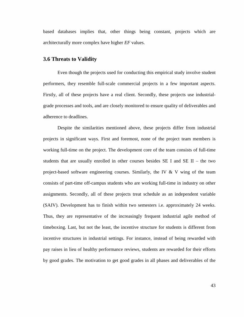
43
based databases implies that, other things being constant, projects which are
architecturally more complex have higher EF values.
3.6 Threats to Validity
Even though the projects used for conducting this empirical study involve student
performers, they resemble full-scale commercial projects in a few important aspects.
Firstly, all of these projects have a real client. Secondly, these projects use industrial-
grade processes and tools, and are closely monitored to ensure quality of deliverables and
adherence to deadlines.
Despite the similarities mentioned above, these projects differ from industrial
projects in significant ways. First and foremost, none of the project team members is
working full-time on the project. The development core of the team consists of full-time
students that are usually enrolled in other courses besides SE I and SE II – the two
project-based software engineering courses. Similarly, the IV & V wing of the team
consists of part-time off-campus students who are working full-time in industry on other
assignments. Secondly, all of these projects treat schedule as an independent variable
(SAIV). Development has to finish within two semesters i.e. approximately 24 weeks.
Thus, they are representative of the increasingly frequent industrial agile method of
timeboxing. Last, but not the least, the incentive structure for students is different from
incentive structures in industrial settings. For instance, instead of being rewarded with
pay raises in lieu of healthy performance reviews, students are rewarded for their efforts
by good grades. The motivation to get good grades in all phases and deliverables of the

44
project may cause students, among other things, to over-specify high-level goals to get
good grades on early deliverables.
These constraints on the full-time availability of team members, duration of the
project, and incentive structure for students may limit the applicability of results of this
empirical study in non-academic contexts. It should not be hard, however, to use the
metrics defined in Section 3.2 to collect and analyze data in industrial settings. The only
prerequisite for using these metrics is the availability of project documentation containing
information about early product goals and detailed product requirements. Using
MBASE/RUP [B. Boehm et al., 2004; Kruchten, 2003] or LeanMBASE/RUP [B. Boehm
et al., 2005; Kruchten, 2003] – the software development process followed by the small
real-client projects analyzed in this study – is, by no means, a requirement for using these
metrics.

45
Chapter 4 From Cloud to Clam
The results of the previous empirical study clearly indicate that for non-functional
requirements there is a magical expansion ratio of 1. One cloud-level LOS goal maps to
exactly one kite-level LOS requirement. This is generally the case because LOS goals
and requirements apply to the total system and not to incremental capabilities. For
functional requirements, however, this concept of a magical expansion ratio does not hold.
The elaboration factor between cloud-level capability goals and kite-level capability
requirements varies across different projects. The other three empirical studies, therefore,
focus solely on the elaboration of functional requirements in order to obtain a deeper
understanding of the reasons for this variation.
This chapter reproduces, with minor modifications, the second empirical study
[Malik, Koolmanojwong, and Boehm, 2009] on requirements elaboration which builds on
the foundation laid by the previous study. This study examines the entire process of
elaboration of functional requirements starting at high-level goals and ending at SLOC.
In terms of the Cockburn metaphor [Cockburn, 2001], it examines all intermediate stages
of elaboration between the cloud and the clam levels.
Unlike the previous empirical study which analyzed project documentation
produced at two different milestones (i.e. LCO and IOC), this study (and all subsequent
empirical studies) examine project documentation produced at the time of one milestone
i.e. IOC. This change obviates the need to make adjustments of the type shown by
Equations 1 and 2 in Section 3.2 and allows using relatively simpler metrics for
measuring requirements elaboration.

46
The experimental setting of this study is described in Section 4.1. This is followed
by an outline of the data collection approach in Section 4.2. Section 4.3 summarizes the
results and discusses the salient aspects of these results. A case study demonstrating the
application of the approach defined in this empirical study on large commercial projects
is presented in Section 4.4.
4.1 Experimental Setting
This empirical study examines multi-level requirements data of 25 small real-
client e-services projects done in the past few years by graduate students studying
software engineering at USC [USC SE I, 2010; USC SE II, 2010]. These projects are
listed in Table 6. Each of these 25 projects was done in two semesters (i.e. 24 weeks) by
a team of 6 to 8 graduate students. Clients of these projects included USC-neighborhood
organizations, USC departments, and USC Center for Systems and Software Engineering
(CSSE) affiliate organizations.
Special care was exercised in selecting projects for this empirical study. To enable
a complete end-to-end comparison of elaboration factors, projects with incomplete
information on any level of requirements were filtered out. Similarly, COTS-intensive
applications, for which requirements data is not readily available at all levels, were not
considered. Thus, each of these 25 projects was a fully-documented custom-development
project. Furthermore, each project followed an architected-agile process [Boehm and
Lane, 2008] such as MBASE [Boehm et al., 2004], LeanMBASE [Boehm et al., 2005], or
Instructional ICM-Sw [Instructional ICM-Sw, 2008].

47
Table 6: Projects used for second empirical study
S# Year Project Name Project Type 1 2004 Online Bibliographies on Chinese Religions Web-based Database 2 2004 Data Mining of Digital Library Usage Data Stand-alone Analysis Tool 3 2004 Data Mining from Report Files Stand-alone Analysis Tool 4 2005 Data Mining PubMed Results Stand-alone Analysis Tool 5 2005 USC Football Recruiting Database Web-based Database 6 2005 Template-based Code Generator Stand-alone Conversion Tool 7 2005 Web-based XML Editing Tool Web-based Editor 8 2005 EBay Notification System Stand-alone Analysis Tool 9 2005 Rule-based Editor Stand-alone Database
10 2005 CodeCount™ Product Line with XML and C++ Stand-alone Analysis Tool 11 2006 USC Diploma Order and Tracking System Web-based Database 12 2006 Student's Academic Progress Application Web-based Database 13 2006 USC CONIPMO Stand-alone Cost Model 14 2007 USC COINCOMO Stand-alone Cost Model 15 2007 BTI Appraisal Projects Web-based Database 16 2007 LAMAS Customer Service Application Web-based Database 17 2007 BID Review System Web-based Database 18 2007 Proctor and Test Site Tracking System Web-based Database 19 2008 Master Pattern Web-based Database 20 2008 Housing Application Tracking System Web-based Database 21 2008 EZBay Stand-alone Analysis Tool 22 2008 AAA Petal Pushers Remote R&D Web-based Database 23 2008 Online Peer Review System for Writing Program Web-based Database 24 2008 The Virtual Assistant Living and Education Program Stand-alone Database 25 2008 Theatre Script Online Database Web-based Database
4.2 Method
Figure 15: Data collection process
1. Define mapping with Cockburn metaphor
2. Identify relevant artifacts
3. Retrieve requirements data from artifacts
4. Normalize requirements data
5. Calculate elaboration factors

48
Figure 15 shows the process followed in collecting data for this empirical study.
Step one involved defining a concrete mapping between the various levels of the
Cockburn metaphor (see Figure 3) and the requirements levels of these e-services
projects. This mapping is shown in Table 7. Each subsequent requirements level builds
on the previous by adding more detail. Capability goals are high-level functional goals of
a project. A typical capability goal taken from one of these 25 projects states: “Data
Analysis: The system will analyze the subsets of data as requested by the user to calculate
the required statistics.” Capability requirements, on the other hand, are more precise
statements about the functional requirements of a project. A typical capability
requirement specifies the pre-conditions, post-conditions, actors, inputs, outputs, sources,
and destinations in addition to a specific textual description. The description of one of the
capability requirements corresponding to the above-mentioned capability goal states:
“The system shall count the number of times each journal appears in the imported
dataset”. Use cases represent behavioral processes which are usually specified in the
UML Use Case Diagram [Booch, Rumbaugh, and Jacobson, 1999] of a system. Use case
steps include “Actor Action” and “System Response” steps in the main scenario as well
as the alternative scenarios of a use case. These do not correspond to messages
exchanged in a UML Sequence Diagram [Booch, Rumbaugh, and Jacobson, 1999].
Table 7: Mapping
Cockburn Metaphor Requirements Level Cloud Capability goals Kite Capability requirements Sea Level Use cases Fish Use case steps Clam SLOC

49
The next step was identification of relevant artifacts that contained data for each
requirements level. Table 8 contains the list of artifacts [B. Boehm et al., 2004; B. Boehm
et al., 2005; Instructional ICM-Sw, 2008] examined for each e-services project.
Information about a project’s high-level capability goals was present in the Operational
Concept Description (OCD) document while its capability requirements were
documented in the System and Software Requirements Definition (SSRD) document. The
System and Software Architecture Description (SSAD) document contained information
on use cases as well as their component steps. SLOC information was available from a
project’s source code. In order to ensure consistency in the presence of multiple versions
of each artifact, it was necessary to get each artifact from the same anchor point
milestone [Boehm, 1996]. For this purpose, the Initial Operational Capability (IOC)
milestone was used since it corresponds to the end of the Construction phase [Kruchten,
2003]. At this point the product is ready to be transitioned to the client.
Step three required retrieving relevant data from these artifacts. Capability goals,
capability requirements, use cases, and use case steps were obtained from inspection of
relevant documents. A project’s SLOC were obtained by running a code counter on its
source code.
Table 8: Relevant artifacts
Requirements Level Artifact Capability goals Operational Concept Description Capability requirements System and Software Requirements Definition Use cases System and Software Architecture Description Use case steps System and Software Architecture Description SLOC Source Code

50
In order to ensure consistency in the level of detail at each requirements level and
to improve the accuracy of analysis, the retrieved data was normalized in the next step.
The normalization of the capability goals of a project included, for instance, merging
related low-level capability goals into one high-level capability goal. As an example, one
of these 25 projects specified “Add an entry”, “Edit an entry”, and “Delete an entry” as
three separate capability goals. During the normalization process, these three capability
goals were merged into one “Manage entry” capability goal. The normalization of
capability requirements involved steps like splitting aggregate requirements into their
individual components and treating each component as a separate capability requirement.
One project, for instance, treated generating five different types of reports as one
capability requirement. During normalization, each of these five types of reports was
counted as a separate capability requirement.
Appendix A contains detailed guidelines for the normalization of high-level
requirements e.g. capability goals and capability requirements. A similar procedure was
followed in normalizing use cases and use case steps. SLOC were normalized by
ensuring that auto-generated code was not counted.
Once the requirements data had been normalized, the final step involved counting
the number of capability goals (CG), capability requirements (CR), use cases (UC), use
case steps (UCS), and SLOC and, thereafter, calculating the elaboration factor for each
pair of consecutive requirements levels. Table 9 displays the formulae used for
calculating the elaboration factors for these e-services projects. As is evident from these
formulae, each elaboration factor is a ratio of the number of requirements at two
consecutive requirements levels. The capability goals-to-capability requirements

51
elaboration factor, for instance, is the ratio of CR and CG. The value of this ratio
indicates the average number of capability requirements obtained as a result of the
elaboration of a single capability goal.
Table 9: Formulae for elaboration factors
Elaboration Stage Cockburn Metaphor E-Services Projects
Elaboration Factor Formula
Cloud-to-Kite Capability Goals-to-Capability Requirements
CG
CR
Kite-to-Sea Level Capability Requirements-to-Use Cases
CR
UC
Sea Level-to-Fish Use Cases-to-Use Case Steps
UC
UCS
Fish-to-Clam Use Case Steps-to-SLOC
UCS
SLOC
4.3 Results and Discussion
Table 10 lists the elaboration factor sets for each of the 25 e-services projects and
Figures 16 – 19 display distributions of the four elaboration factors. This data is
summarized in Table 11. On average, a capability goal is elaborated into about two or
three capability requirements, a capability requirement maps to a single use case, a use
case has about seven steps, and a use case step is implemented by about 67 SLOC.

52
Table 10: Elaboration factor sets for each project
S# Project Name
CG
CR
CR
UC
UC
UCS
UCS
SLOC
1 Online Bibliographies on Chinese Religions 3.00 1.00 7.89 64.75 2 Data Mining of Digital Library Usage Data 3.67 0.18 9.00 118.56 3 Data Mining from Report Files 3.00 0.43 6.00 40.72 4 Data Mining PubMed Results 3.50 0.29 7.00 5.89 5 USC Football Recruiting Database 1.83 0.91 8.90 26.80 6 Template-based Code Generator 2.50 0.40 3.50 278.57 7 Web-based XML Editing Tool 1.33 1.25 5.80 140.52 8 EBay Notification System 2.75 0.82 2.44 38.27 9 Rule-based Editor 2.00 0.75 4.83 32.17
10 CodeCount™ Product Line with XML and C++ 1.20 0.08 15.00 96.07 11 USC Diploma Order and Tracking System 1.60 1.22 3.45 31.63 12 Student's Academic Progress Application 1.60 0.89 3.63 15.76 13 USC CONIPMO 1.29 0.90 5.44 108.92 14 USC COINCOMO 2.80 0.38 6.67 199.15 15 BTI Appraisal Projects 3.20 1.00 5.75 23.74 16 LAMAS Customer Service Application 1.00 1.00 6.57 67.72 17 BID Review System 1.17 1.29 13.78 42.58 18 Proctor and Test Site Tracking System 1.90 0.84 8.38 74.46 19 Master Pattern 1.75 1.57 5.32 100.15 20 Housing Application Tracking System 3.00 2.88 8.63 16.84 21 EZBay 3.25 0.88 5.33 60.51 22 AAA Petal Pushers Remote R&D 4.17 1.00 6.48 4.29 23 Online Peer Review System for Writing Program 3.57 0.93 9.72 38.72 24 The Virtual Assistant Living and Education Program 3.57 0.88 9.68 16.49 25 Theatre Script Online Database 2.83 0.60 7.25 29.49
Capability Requirements/Capability Goals
0.00
0.50
1.00
1.50
2.00
2.50
3.00
3.50
4.00
4.50
16 17 10 13 7 11 12 19 5 18 9 6 8 14 25 1 3 20 15 21 4 23 24 2 22
Project Number
CR
/CG
Figure 16: CG
CR
distribution

53
Use Cases/Capability Requirements
0.00
0.50
1.00
1.50
2.00
2.50
3.00
3.50
10 2 4 14 6 3 25 9 8 18 24 21 12 13 5 23 1 15 16 22 11 7 17 19 20
Project Number
UC
/CR
Figure 17: CR
UC
distribution
Use Case Steps/Use Cases
0.00
2.00
4.00
6.00
8.00
10.00
12.00
14.00
16.00
8 11 6 12 9 19 21 13 15 7 3 22 16 14 4 25 1 18 20 5 2 24 23 17 10
Project Number
UC
S/U
C
Figure 18: UC
UCS
distribution

54
SLOC/Use Case Steps
0.00
50.00
100.00
150.00
200.00
250.00
300.00
22 4 12 24 20 15 5 25 11 9 8 23 3 17 21 1 16 18 10 19 13 2 7 14 6
Project Number
SL
OC
/UC
S
Figure 19: UCS
SLOC
distribution
Table 11: Summary of elaboration results
Elaboration Factors
Statistic
CG
CR
CR
UC
UC
UCS
UCS
SLOC
Average 2.46 0.89 7.06 66.91 Median 2.75 0.89 6.57 40.72 Standard Deviation 0.94 0.55 2.97 64.46
The capability requirements-to-use cases elaboration factor - CR
UC - is almost one.
In other words, on average, use cases were expressed at almost the same level as
capability requirements. This discrepancy may be explained by the students’ desire to get
better grades. This desire motivated them to specify capability requirements at the same
level as use cases. This also identifies an opportunity to save valuable time during the
development of such projects. The absence of little or no value addition from the
capability requirements level to the use cases level signals that activities in one of these
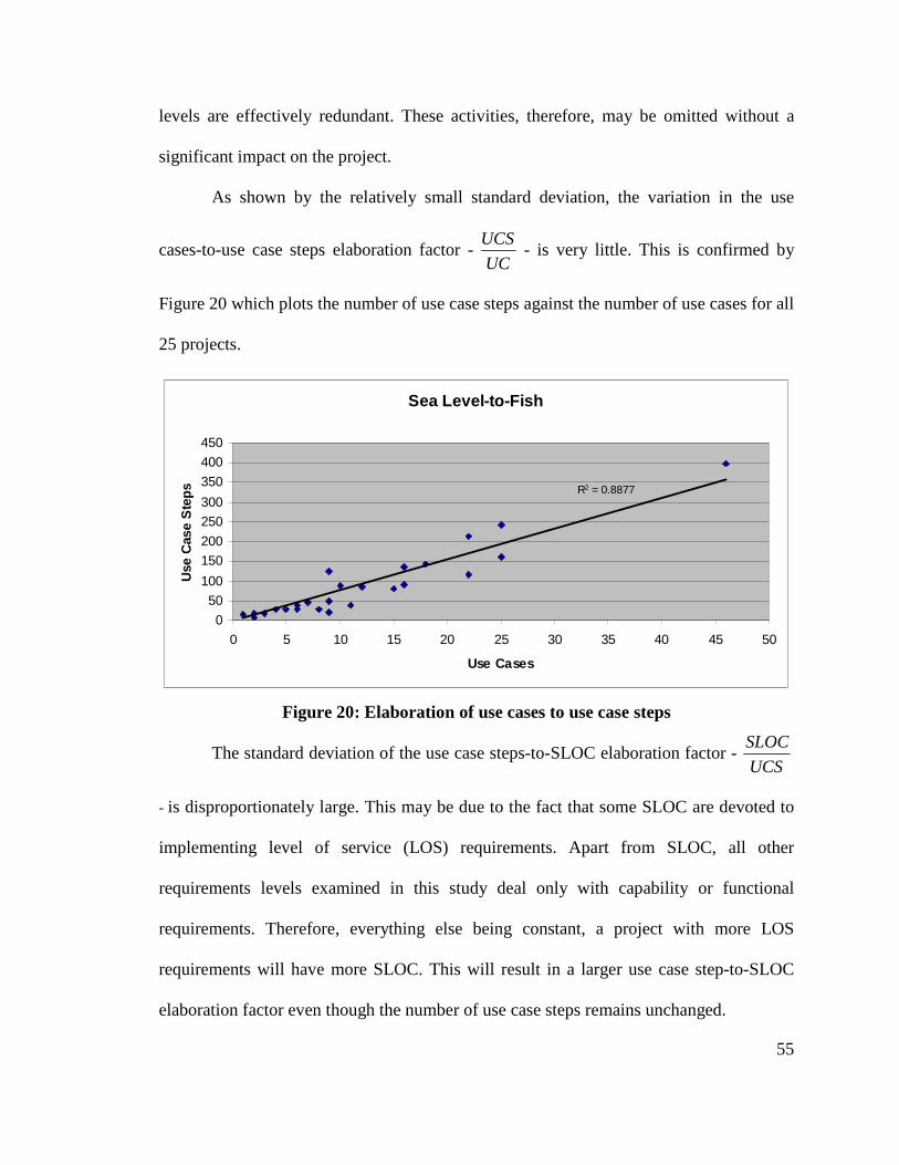
55
levels are effectively redundant. These activities, therefore, may be omitted without a
significant impact on the project.
As shown by the relatively small standard deviation, the variation in the use
cases-to-use case steps elaboration factor - UC
UCS - is very little. This is confirmed by
Figure 20 which plots the number of use case steps against the number of use cases for all
25 projects.
Sea Level-to-Fish
R2 = 0.8877
0
50
100
150
200
250
300
350
400
450
0 5 10 15 20 25 30 35 40 45 50
Use Cases
Use
Cas
e S
tep
s
Figure 20: Elaboration of use cases to use case steps
The standard deviation of the use case steps-to-SLOC elaboration factor - UCS
SLOC
- is disproportionately large. This may be due to the fact that some SLOC are devoted to
implementing level of service (LOS) requirements. Apart from SLOC, all other
requirements levels examined in this study deal only with capability or functional
requirements. Therefore, everything else being constant, a project with more LOS
requirements will have more SLOC. This will result in a larger use case step-to-SLOC
elaboration factor even though the number of use case steps remains unchanged.

56
The information summarized in Table 11 can be easily used to estimate the SLOC
of a similar new e-service project at the time of its inception. Once the high-level
capability goals of this project have been determined, the following formula can be used
to estimate the number of SLOC for this project:
Equation 1: UCS
SLOC
UC
UCS
CR
UC
CG
CRCGSLOC ××××=
The first term on the right-hand side of Equation 1 is the number of capability goals and
the remaining four terms represent the elaboration factors defined in Table 9.
Consider, for instance, a new e-service project that has identified 5 high-level
capability goals at inception. The most likely SLOC for this project can be estimated by
using Equation 1 and plugging-in the value of CG (= 5) along with the average-values of
elaboration factors shown in Table 11.
Most Likely SLOC = 5 * 2.46 * 0.89 * 7.06 * 66.91 ≈ 5171
A one-standard deviation SLOC-range can also be calculated for this project using the
standard deviations shown in Table 11:
Minimum SLOC = 5 * (2.46 – 0.94) * (0.89 – 0.55) * (7.06 – 2.97) * (66.91 – 64.46)
≈ 26
Maximum SLOC = 5 * (2.46 + 0.94) * (0.89 + 0.55) * (7.06 + 2.97) * (66.91 + 64.46)
≈ 32, 256
4.4 Requirements Elaboration of Commercial Projects
This technique of analyzing a project’s multi-level requirements data to determine
its set of elaboration factors can be applied to large commercial projects as well. An
opportunity to conduct such an analysis was provided by ballpark data in [Hopkins and

57
Jenkins, 2008] on multiple requirements levels of a certain category of large IBM
projects. Table 12 summarizes this data.
Table 12: Multi-level requirements data of large IBM projects
Requirements Level Number of Requirements Business events 50 Use cases 200 Main steps 1, 500 Detailed operations 20, 000 SLOC 1, 500, 000
Each requirements level shown in Table 12 can be mapped to an altitude level of
the Cockburn metaphor. Table 13 shows this mapping along with the set of elaboration
factors of these large IBM projects. On average, a business event is elaborated into four
use cases, a use case contains about seven or eight main steps, a main step is expressed
by about thirteen detailed operations, and a detailed operation is implemented by seventy-
five SLOC.
Table 13: Elaboration factors of large IBM projects
Elaboration Stage Cockburn Metaphor Large IBM Projects
Elaboration Factor
Cloud-to-Kite Business Events-to-Use Cases 4.00 Kite-to-Sea Level Use Cases-to-Main Steps 7.50 Sea Level-to-Fish Main Steps-to-Detailed Operations 13.33 Fish-to-Clam Detailed Operations-to-SLOC 75.00
Elaboration factors obtained from this analysis can be helpful in early sizing and
cost estimation of similar future projects. Using these elaboration factors, an estimate of
the size of a new project can be obtained as early as the inception stage. Consider, for
instance, a similar large IBM project that identifies 60 business events at the time of
inception. Based on the elaboration factors in Table 13, a rough sizing of this project
would be about (60 * 4 * 7.5 * 13.33 * 75 ≈) 1, 800 KSLOC.

58
However, even within IBM, one would have to be careful about binding such an
estimate into a firm commitment. If the project is highly similar, much of its software
could be reused from previous projects at much less cost. If it is dissimilar, it is not clear
how to adjust the estimate. The strongest approach would be to obtain distributions of
elaboration factors such as the ones shown for e-services projects in Figures 16 – 19, and
to determine confidence intervals for SLOC estimates based on these distributions for
one’s own organization.

59
Chapter 5 Efficacy of COCOMO II Cost Drivers in Predicting
Elaboration Profiles
The first empirical study (see Chapter 3) identified project precedentedness as one
of the potential determinants of the variation in the first stage of requirements elaboration.
Coincidentally, precedentedness (PREC) is one of the cost drivers of COCOMO II
[Boehm et al., 2000]. Can PREC and other COCOMO II cost drivers be used to predict
the variations in the different stages of elaboration?
This chapter attempts to answer the above question. It reproduces, with minor
modifications, the third empirical study [Malik and Boehm, 2010] on requirements
elaboration. The empirical setting of this study is the same as the second study as it uses
the same set of 25 small e-services projects (see Table 6). The purpose of this study is to
determine the efficacy of COCOMO II cost drivers in predicting the elaboration profile
(EP) of a project. A project’s EP consists of the elaboration factors for all stages of
elaboration. Due to the pairing of consecutive requirements levels in calculating
elaboration factors, a project which expresses requirements at n different levels has n – 1
elaboration factors in its EP.
Section 5.1 describes the process for determining the COCOMO II cost driver
ratings. Data analysis results are reported in Section 5.2 along with a commentary on the
salient aspects of these results. Section 5.3 concludes this chapter with a discussion of the
possible reasons for these results.
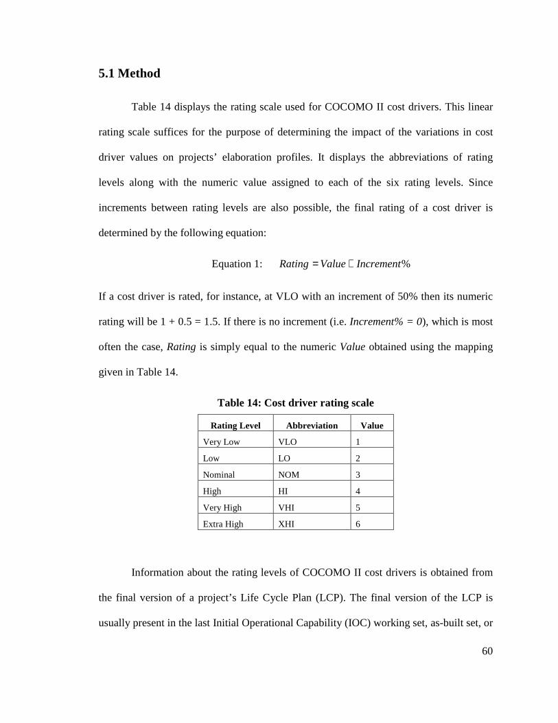
60
5.1 Method
Table 14 displays the rating scale used for COCOMO II cost drivers. This linear
rating scale suffices for the purpose of determining the impact of the variations in cost
driver values on projects’ elaboration profiles. It displays the abbreviations of rating
levels along with the numeric value assigned to each of the six rating levels. Since
increments between rating levels are also possible, the final rating of a cost driver is
determined by the following equation:
Equation 1: %IncrementValueRating +=
If a cost driver is rated, for instance, at VLO with an increment of 50% then its numeric
rating will be 1 + 0.5 = 1.5. If there is no increment (i.e. Increment% = 0), which is most
often the case, Rating is simply equal to the numeric Value obtained using the mapping
given in Table 14.
Table 14: Cost driver rating scale
Rating Level Abbreviation Value
Very Low VLO 1
Low LO 2
Nominal NOM 3
High HI 4
Very High VHI 5
Extra High XHI 6
Information about the rating levels of COCOMO II cost drivers is obtained from
the final version of a project’s Life Cycle Plan (LCP). The final version of the LCP is
usually present in the last Initial Operational Capability (IOC) working set, as-built set, or

61
the final deliverables of the project. The rationale for choosing the final version of LCP is
two-fold. Firstly, the elaboration profiles were obtained using documents produced at the
IOC anchor point milestone [Boehm, 1996] which maps to the end of the construction
phase. Thus, in order to ensure consistency with the elaboration profiles, COCOMO II
cost driver ratings are also derived from the same milestone. Secondly, it is important to
use stabilized ratings of cost drivers. The final version of the LCP contains ratings that
have stabilized after evolution over the course of the project.
Finding the numeric ratings of a project’s five scale factors – PREC, FLEX,
RESL, TEAM, and PMAT – is a straight forward process. This is primarily because these
scale factors apply to the project as a whole. Once the rating levels of these scale factors
have been obtained from the LCP, all that needs to be done is to map the rating levels to
the numeric values using Table 14 and then use Equation 1 to get the final rating. Even
though the multiplicative SCED cost driver also applies to the project as a whole, it can
be easily omitted from this particular analysis. This is because all 25 projects examined in
this study use the SAIV process model and thus have the same value (i.e. NOM) for the
SCED cost driver.
Determining the numeric ratings of the multiplicative cost drivers (excluding
SCED) requires more effort. The reason for this is that these multiplicative cost drivers
apply to the individual modules of the project. In other words, each module of the project
has its own separate list of multiplicative cost driver ratings. In order to reconcile this
difference between the applicability of project-wide scale factors and module-wide
multiplicative cost drivers, module-wide cost drivers are weighted by module size to
come up with a project-wide rating. The following formula is used for this conversion:

62
Equation 2:
∑
∑
=
=
×=
n
ii
n
iii
ModuleSize
ModuleSizengModuleRatigojectRatin
1
1Pr
In Equation 2, n represents the number of modules in the project. Modules that are
bigger in size have more impact on the ProjectRating vis-à-vis smaller modules.
Consider, for instance, a project that has three modules – M1, M2, and M3 – with sizes
100 KSLOC, 200 KSLOC, and 300 KSLOC respectively. If CPLX rating levels for M1,
M2, and M3 are LO, NOM, and HI respectively, then using Table 14 (and assuming
Increment% = 0) the overall project CPLX rating is given by:
33.3600
2000
)300200100(
)3004()2003()1002( ==++
×+×+×
5.2 Results
Tables 15 through 19 summarize the COCOMO II cost driver ratings for each of
the 25 small real-client projects. These ratings have been calculated using the procedure
described in the previous section. For ease of reference, the first column – S# – in these
tables maps to the first column of Table 6.
As a first step towards determining the utility of COCOMO II cost drivers in
predicting the elaboration profile of a project, a simple regression analysis is carried out.
The individual correlation between each of the 4 elaboration factors (i.e. CG
CR,
CR
UC,
UC
UCS, and
UCS
SLOC) and each of the 21 COCOMO II cost drivers (i.e. 5 scale factors and
16 multiplicative cost drivers) is determined. Needless to say, in all of these regression

63
analyses, the elaboration factor acts as the response variable while the cost driver acts as
the predictor. All in all, 4 x 21 = 84 correlations are calculated.
Table 15: COCOMO II scale factor ratings
Scale Factors
S# PREC FLEX RESL TEAM PMAT 1 3.00 5.00 5.00 3.00 3.00 2 3.00 3.00 4.00 5.00 3.00 3 3.00 4.00 5.00 4.00 3.00 4 3.00 2.00 4.00 4.00 3.00 5 3.00 4.00 4.00 4.00 3.00 6 3.00 2.00 3.00 4.00 2.00 7 3.00 3.00 4.00 3.00 3.00 8 3.00 3.00 4.00 3.00 3.00 9 4.00 3.00 4.00 3.00 4.00
10 2.00 2.00 3.00 5.00 1.00 11 3.00 3.00 4.00 3.00 3.00 12 4.00 2.00 4.00 4.00 3.00 13 6.00 2.00 4.00 2.00 3.00 14 2.00 5.00 4.00 4.00 3.00 15 3.25 4.00 3.00 3.00 3.00 16 2.00 3.00 3.00 4.00 3.00 17 2.00 3.00 3.00 4.00 3.00 18 3.00 3.00 4.00 4.00 3.00 19 3.00 4.00 3.00 4.00 3.00 20 3.00 3.00 3.00 1.00 4.00 21 2.00 3.00 3.00 4.00 3.00 22 4.00 4.00 4.00 4.00 3.00 23 3.00 4.00 4.00 4.00 3.00 24 4.00 3.00 3.00 3.00 4.00 25 3.00 4.00 4.00 3.00 3.00

64
Table 16: COCOMO II product factor ratings
Product Factors
S# RELY DATA CPLX RUSE DOCU 1 2.00 2.14 2.89 2.00 2.64 2 3.00 4.00 2.56 2.71 3.00 3 3.00 2.96 3.30 2.09 5.00 4 3.00 3.50 2.00 3.00 4.00 5 3.00 3.00 3.14 3.00 3.07 6 2.00 2.00 3.95 3.00 5.00 7 3.20 3.00 2.80 2.00 3.40 8 3.60 3.00 2.80 2.00 3.40 9 3.31 2.00 3.00 2.00 5.00
10 3.77 3.23 2.68 2.00 3.00 11 3.00 3.00 3.00 3.00 3.00 12 3.87 3.00 3.17 3.00 3.30 13 4.00 3.00 2.00 2.00 2.00 14 2.00 2.00 3.00 4.00 3.00 15 1.70 2.00 2.63 2.66 3.34 16 2.00 2.00 1.54 3.00 4.00 17 3.00 3.00 3.21 3.00 4.00 18 3.00 2.00 3.00 2.00 3.00 19 3.74 2.89 2.94 2.13 2.89 20 3.00 3.00 3.27 3.00 2.72 21 2.71 2.71 3.00 2.00 4.00 22 3.06 2.00 3.09 2.00 3.00 23 3.00 2.00 3.27 2.00 2.00 24 4.00 2.07 2.38 3.00 3.00 25 2.74 2.27 3.03 2.00 3.00

65
Table 17: COCOMO II platform factor ratings
Platform Factors
S# TIME STOR PVOL 1 3.00 3.00 2.00 2 3.00 3.33 4.00 3 2.00 2.00 2.00 4 3.33 3.00 3.00 5 3.86 3.93 2.14 6 3.45 2.26 2.00 7 3.00 3.00 3.00 8 3.00 3.00 3.00 9 3.00 3.00 2.00
10 3.00 3.00 3.00 11 3.00 3.00 2.00 12 3.00 3.00 3.00 13 3.00 3.00 2.00 14 3.00 3.00 3.00 15 3.00 3.00 2.00 16 3.00 3.00 3.00 17 3.00 3.00 2.00 18 3.00 3.00 2.00 19 3.00 3.00 2.00 20 3.00 3.00 2.52 21 3.29 3.00 2.00 22 3.00 3.00 2.00 23 3.00 3.00 2.00 24 3.00 3.00 2.00 25 3.00 2.30 1.81

66
Table 18: COCOMO II personnel factor ratings
Personnel Factors
S# ACAP PCAP PCON APEX PLEX LTEX 1 3.00 4.00 2.00 3.00 2.00 2.00 2 3.00 4.00 2.00 2.72 2.00 4.00 3 3.00 3.00 3.00 1.00 2.00 2.00 4 3.00 3.00 1.00 3.00 4.00 3.00 5 3.00 2.93 5.00 1.93 1.93 2.93 6 2.77 2.45 1.00 1.77 2.00 3.00 7 2.60 3.00 3.00 2.00 3.00 3.00 8 2.60 3.60 4.00 2.00 3.00 3.00 9 4.00 3.00 2.00 4.00 3.00 4.00
10 3.00 4.00 2.00 4.00 5.00 4.00 11 3.00 3.00 3.00 3.00 3.00 3.00 12 3.00 3.83 3.00 3.83 3.00 3.00 13 4.00 4.00 3.00 5.00 5.00 4.11 14 4.00 3.00 1.00 3.00 3.00 3.00 15 2.66 2.66 4.00 2.32 3.32 2.32 16 3.00 3.00 3.00 2.00 2.00 3.00 17 3.00 3.00 2.00 3.00 2.89 3.00 18 3.00 4.00 2.00 4.00 3.00 2.00 19 4.00 4.00 2.00 3.00 2.00 3.00 20 3.53 2.00 2.00 2.00 2.00 2.00 21 4.00 4.00 2.00 3.00 3.00 3.00 22 5.00 5.00 3.00 3.00 2.84 2.96 23 4.52 4.52 5.00 4.04 4.04 4.04 24 3.00 4.62 3.00 4.62 3.00 4.62 25 3.00 3.00 4.00 3.15 3.00 3.00

67
Table 19: COCOMO II project factor ratings
Project Factors
S# TOOL SITE 1 3.00 3.00 2 4.00 3.00 3 3.00 5.00 4 4.00 4.00 5 2.93 4.00 6 4.00 5.00 7 3.00 3.00 8 3.00 5.00 9 5.00 4.00
10 3.00 3.00 11 3.00 4.00 12 3.30 3.00 13 5.00 4.00 14 4.00 4.00 15 3.00 5.22 16 3.00 3.00 17 3.00 4.00 18 3.00 4.00 19 2.00 5.00 20 3.00 1.00 21 3.00 5.00 22 2.00 5.00 23 3.00 5.00 24 4.00 4.00 25 4.00 4.00

68
Tables 20 through 23 summarize the results of these simple regression analyses.
These tables have been sorted in descending order of the correlation strength. In other
words, COCOMO II drivers having a higher value of the coefficient of determination
(R2) appear above those with lower values. The first column of these tables – Rank –
indicates the rank of the cost driver with respect to its correlation strength. The column
labeled “+/-” specifies the direction of the relationship between the elaboration factor and
the cost driver as indicated by the sign of the slope coefficient of the fitted mean function
using ordinary least squares. A “+” indicates a positive relationship while a “-” signifies a
negative or inverse relationship. The last column – Type – displays the category of the
COCOMO II cost driver i.e. scale factor, product factor, platform factor, personnel factor,
or project factor.

69
Table 20: Correlation between CG
CR
and COCOMO II cost drivers
Rank R2 +/- COCOMO II Driver Type
1 0.1283 + FLEX Scale Factor
2 0.0877 + ACAP Personnel Factor
3 0.0793 + PMAT Scale Factor
4 0.0724 + SITE Project Factor
5 0.0712 + PCAP Personnel Factor
6 0.0455 - RELY Product Factor
7 0.0345 + RESL Scale Factor
8 0.0225 - DATA Product Factor
9 0.0214 + CPLX Product Factor
10 0.0174 - PLEX Personnel Factor
11 0.0165 - STOR Platform Factor
12 0.0073 - APEX Personnel Factor
13 0.0053 - TIME Platform Factor
14 0.0048 - DOCU Product Factor
15 0.0029 + PREC Scale Factor
16 0.0015 - PVOL Platform Factor
17 0.0009 - PCON Personnel Factor
18 0.0009 - RUSE Product Factor
19 0.0008 - LTEX Personnel Factor
20 0.0005 - TOOL Project Factor
21 9.00E-06 + TEAM Scale Factor

70
Table 21: Correlation between CR
UC
and COCOMO II cost drivers
Rank R2 +/- COCOMO II Driver Type
1 0.4707 - TEAM Scale Factor
2 0.2694 + PMAT Scale Factor
3 0.1531 - SITE Project Factor
4 0.1425 - TOOL Project Factor
5 0.1233 - LTEX Personnel Factor
6 0.0895 - PLEX Personnel Factor
7 0.0806 - RESL Scale Factor
8 0.0739 - DOCU Product Factor
9 0.0645 - PVOL Platform Factor
10 0.0593 - PCAP Personnel Factor
11 0.0313 + STOR Platform Factor
12 0.0235 + ACAP Personnel Factor
13 0.0193 + CPLX Product Factor
14 0.0188 - APEX Personnel Factor
15 0.0128 + PCON Personnel Factor
16 0.0119 + FLEX Scale Factor
17 0.0054 + PREC Scale Factor
18 0.0048 + RELY Product Factor
19 0.0013 + RUSE Product Factor
20 0.0011 - DATA Product Factor
21 0.0002 + TIME Platform Factor

71
Table 22: Correlation between UC
UCS
and COCOMO II cost drivers
Rank R2 +/- COCOMO II Driver Type
1 0.1148 - PREC Scale Factor
2 0.1016 - SITE Project Factor
3 0.082 + TEAM Scale Factor
4 0.0652 + APEX Personnel Factor
5 0.0635 - DOCU Product Factor
6 0.0633 - PMAT Scale Factor
7 0.057 + PLEX Personnel Factor
8 0.0558 + STOR Platform Factor
9 0.0551 - RESL Scale Factor
10 0.0467 + LTEX Personnel Factor
11 0.0306 + PCAP Personnel Factor
12 0.0192 + DATA Product Factor
13 0.0117 - TOOL Project Factor
14 0.0109 + RELY Product Factor
15 0.005 - CPLX Product Factor
16 0.0042 + PVOL Platform Factor
17 0.0018 - PCON Personnel Factor
18 0.0007 + FLEX Scale Factor
19 0.0007 + RUSE Product Factor
20 0.0006 + TIME Platform Factor
21 6.00E-05 - ACAP Personnel Factor

72
Table 23: Correlation between UCS
SLOC
and COCOMO II cost drivers
Rank R2 +/- COCOMO II Driver Type
1 0.2265 - PCON Personnel Factor
2 0.2058 - PMAT Scale Factor
3 0.0868 - RELY Product Factor
4 0.0579 + TOOL Project Factor
5 0.0526 - STOR Platform Factor
6 0.0514 + TEAM Scale Factor
7 0.0486 + CPLX Product Factor
8 0.0401 + RUSE Product Factor
9 0.0391 + PVOL Platform Factor
10 0.0318 - PCAP Personnel Factor
11 0.026 - PREC Scale Factor
12 0.0238 + DOCU Product Factor
13 0.0213 - APEX Personnel Factor
14 0.0201 + TIME Platform Factor
15 0.0184 - RESL Scale Factor
16 0.0086 - PLEX Personnel Factor
17 0.008 - DATA Product Factor
18 0.0071 - FLEX Scale Factor
19 0.0066 - ACAP Personnel Factor
20 0.0062 + LTEX Personnel Factor
21 0.0033 + SITE Project Factor

73
Table 20 shows the simple correlation between the first elaboration factor - CG
CR -
and each of the 21 cost drivers. CG
CR represents the elaboration of capability goals (CG)
into capability requirements (CR). While all correlations are weak, CG
CR and FLEX have
the strongest correlation i.e. 0.1283.
Correlations of cost drivers with CR
UC are shown in Table 21.
CR
UC is the second
elaboration factor which measures the elaboration of capability requirements (CR) into
use cases (UC). CR
UC has the highest correlation with TEAM (0.4707) followed by PMAT
(0.2694), SITE (0.1531), TOOL (0.1425), and LTEX (0.1233). Correlations with the rest
of the cost drivers are weak.
The third elaboration factor - UC
UCS - quantifies the elaboration of use cases (UC)
into use case steps (UCS). Table 22 displays the correlations of cost drivers with UC
UCS.
All correlations are weak. However, correlations with PREC (0.1148) and SITE (0.1016)
are relatively stronger.
Table 23 presents the correlations of cost drivers with the last elaboration factor
i.e. UCS
SLOC.
UCS
SLOC measures the elaboration of use case steps (UCS) into source lines of
code (SLOC). In this final stage of elaboration, PCON (0.2265) and PMAT (0.2058) are
the only cost drivers which have correlations worth mentioning.

74
In the second step, multiple regression analysis (which uses one response and
multiple predictors) is used to determine the utility of COCOMO II cost drivers in
predicting the elaboration profile of a project. This involves identifying the cost drivers
pertinent to each stage of elaboration. This list of relevant cost drivers is presented in
Table 24. In this table, each stage is assigned a number for later reference and is labeled
using the Cockburn altitude metaphor [Cockburn, 2001].
Table 24: COCOMO II cost drivers relevant at each elaboration stage
Elaboration Stage
(Cockburn Metaphor)
Relevant Cost Drivers
Stage 1: Capability Goals to Capability Requirements
(Cloud to Kite)
ACAP, APEX, DOCU, FLEX, PREC, RESL, SITE, TEAM
Stage 2: Capability Requirements to Use Cases
(Kite to Sea Level)
ACAP, APEX, PCON, PREC
Stage 3: Use Cases to Use Case Steps
(Sea Level to Fish)
ACAP, APEX, CPLX, DOCU, PCON, PREC
Stage 4: Use Case Steps to SLOC
(Fish to Clam)
APEX, CPLX, LTEX, PCAP, PCON, PLEX, PREC, PVOL, RELY, RUSE, STOR, TIME, TOOL
At each stage of elaboration, cost drivers are short-listed based on their perceived
applicability at that stage. Applications experience and precedentedness can influence
elaboration at each stage thus APEX and PREC are listed as potential predictors in all
four stages. Personnel continuity (PCON) is only relevant after the first stage of
elaboration. Thus, PCON appears in all stages except the first. Required software
reliability (RELY) deals with level-of-service (LOS) or non-functional requirements and
is, therefore, not considered at all. Process maturity (PMAT) is omitted from all four
stages since each of the 25 projects is done by teams of graduate students that are
approximately at the same level of process maturity. Similar reasoning is used to short-

75
list the other cost drivers. As a rule of thumb, scale factors are more relevant in earlier
stages of elaboration while product factors, platform factors, and project factors are more
relevant at later stages. The relevance of personnel factors varies from stage to stage.
Programmer capability (PCAP), for instance, is only relevant at the last stage of
elaboration which deals with SLOC. Analyst capability (ACAP), on the other hand, is
relevant in all stages except the last.
Table 25 summarizes the results of the multiple regression analyses conducted
using the short-listed predictors shown in Table 24. Appendix B contains the details of
this multiple regression analyses performed using the R statistical computing
environment [R Development Core Team, 2007]. The low values of the multiple
correlation coefficients (multiple R2) indicate very weak predictive power of the short-
listed cost drivers. Moreover, the low significance levels (high p-values) signify very
strong evidence in favor of the null hypothesis that the means of the elaboration factors
do not depend on any of their respective short-listed cost drivers.
Table 25: Results of multiple regression analysis
Elaboration Stage Multiple R2 P-value
Stage 1: Capability Goals to Capability Requirements 0.223 0.784
Stage 2: Capability Requirements to Use Cases 0.092 0.731
Stage 3: Use Cases to Use Case Steps 0.373 0.159
Stage 4: Use Case Steps to SLOC 0.547 0.493
5.3 Discussion
Results reported in the previous section clearly imply that there is no magical
formula for predicting the elaboration profile of a project using only the information
contained in the COCOMO II cost drivers. Correlations obtained using the simple and

76
multiple regression analyses are weak indicating that the variance of cost drivers cannot
adequately explain the variance in elaboration factors. This weak predictive power of the
COCOMO II cost drivers may be due to a number of confounding factors.
First and foremost, the accuracy of data needs to be considered. [Malik,
Koolmanojwong, and Boehm, 2009] found that it was necessary to normalize multi-level
requirements data in order to obtain consistent elaboration profiles. Therefore, it may be
necessary to normalize COCOMO II cost driver ratings across these 25 projects. In fact,
concrete evidence already points in favor of this. While obtaining the cost driver ratings,
it was observed that different teams had assigned different rating levels for PCON even
though they had cited the same rationale. Similarly, even though all student teams were
approximately at the same level of process maturity, a number of different rating levels
were noticed for PMAT. Such occurrences clearly indicate the need for having a list of
guiding principles to assist student teams in selecting cost drivers’ rating levels. This
would help a great deal in obtaining consistent ratings of cost drivers across different
projects.
Another potential confounding factor is the students’ incentive structure. Unlike
the individuals involved in industry projects, team members of projects undertaken in
academia are motivated by the desire to get good grades in each deliverable. A natural
consequence of this is over-specification of information. For instance, teams may
document the capability goals in the Operational Concept Description document at the
level of detail of capability requirements. This practice easily corrupts the elaboration
data.

77
Last, but certainly not the least, the variation amongst the clients of these projects
may have played a significant role in the results obtained. As found out by interviewing
the teaching assistants responsible for grading these projects, not all clients wanted quick
feedback in the form of prototypes and screen shots. The demand for quick feedback may
also lead to an over-specification of information at higher levels of requirements. This, in
turn, spoils the elaboration data. The same interview also asked the teaching assistants to
rank the clients on the CRACKD – collaborative, representative, authorized, committed,
knowledgeable, and decisive – characteristics using a scale of 1 (least) to 5 (most).
CRACKD is a slightly augmented version of the CRACK customer characteristics
mentioned in [Boehm and Turner, 2004]. Decisiveness measures the ability of the client
to state requirements that are final and not subject to later modification. As expected,
each client had his/her own CRACKD profile. These client characteristics may also be
responsible for some of the variation in the elaboration profiles. A client that is more
representative and knowledgeable, for instance, may provide more information upfront
leading to lower elaboration factors at higher levels of requirements. On the other hand, a
project with a less decisive client may experience greater elaboration in the earlier stages.

78
Chapter 6 Comparative Analysis of Requirements Elaboration
This chapter reproduces, with minor modifications, the fourth and final empirical
study [Malik, Boehm, Ku, and Yang, 2010] on requirements elaboration. This study uses
a novel approach to determine the elaboration profiles of different versions of an
industrial product. To get further insights into the process of requirements elaboration,
these elaboration profiles are compared with the elaboration profiles obtained in the
second empirical study.
Section 6.1 presents the empirical setting of this study while Section 6.2 describes
the data collection method. The results of data analysis are shown in Section 6.3 which
also discusses the salient aspects of these results. Section 6.4 compares the results of this
study with the results of the second empirical study. Section 6.5 summarizes the major
findings and identifies the main threats to validity.
6.1 Empirical Setting
This empirical study focuses on analyzing the requirements elaboration of an
industrial software process management product called SoftPM [Wang and Li, 2005]
which was developed by a CMMI Maturity Level 4 [Chrissis, Konrad, and Shrum, 2006]
Chinese software company. This product has been in the market for over 7 years and
more than 300 Chinese commercial software organizations use this product to manage
their software processes. About 30 developers and testers have participated in the
iterative development of SoftPM.

79
SoftPM is a web-based Java EE [Jendrock et al., 2006] application with four main
architectural tiers i.e. presentation, control, business logic, and data persistence.
Currently, SoftPM contains more than 600 KSLOC. It has four main modules viz. system
management, project management, measurement and analysis, and process asset
management.
6.2 Data Collection
The first step in collecting the required data was to identify all versions of SoftPM
that had complete documentation including source code files. Complete documentation is
required to extract information about the number of requirements at each level of the
requirements hierarchy. Five versions satisfied this constraint.
Table 26: Requirements levels of SoftPM
S# Requirements Level Cockburn Metaphor
1 Capability Goals (CG) Cloud
2 Capability Requirements (CR) Kite
3 Use Cases (UC) Sea
4 Use Case Steps (UCS) Fish
5 Source Lines of Code (SLOC) Clam
Once the relevant versions had been shortlisted, the next step was to identify the
different levels at which requirements of SoftPM had been expressed in these versions.
These different levels are shown in Table 26. To facilitate visualization of the amount of
detail contained in these levels, a mapping of each requirements level to a level in the
Cockburn altitude metaphor [Cockburn, 2001] is also shown in Table 26. Capability
goals, for instance, contain the least amount of detail and are, therefore, mapped to the

80
cloud level of the Cockburn metaphor. SLOC, on the other hand, map to the lowest level
(i.e. clam) since they cannot be elaborated any further.
Determining the number of requirements at each of these five levels for each of
the five versions of SoftPM entails dealing with the fact that there is considerable overlap
amongst versions. Later versions may not only add brand new CG but may also elaborate
the CG added by previous versions. For example, consider the scenario shown in Figure
21. In this simplified hypothetical scenario, a product has only two versions i.e. V1 and
V2. The second version (V2) adds more functionality to the first (V1). V1 specified two
CG i.e. CG1 and CG2. V2 inherits these two CG and specifies one additional CG i.e.
CG3. Besides this, V2 also adds a new CR – CR4 – to CG1. These new additions in V2
have been shown in bold in Figure 21.
Figure 21: Example scenario depicting overlaps amongst versions
V1
CG1
CR1
CR2
CR3
CG2
CR1
CR2
V2
CG1
CR1
CR2
CR3
CG2
CR1
CR2
CG3
CR1
CR2
CR3
CR4

81
Figure 22: Example scenario after removing overlaps amongst versions
The addition of a completely new CG – CG3 – does not pose any problems for
measuring elaboration since the hierarchies of the incumbent CG remain unmodified.
Complications arise, however, when a change is made to the hierarchy of an overlapping
CG. This is exemplified by the addition of CR4 to the hierarchy of CG1 in V2. This
change to the hierarchy of an overlapping CG implies that this CG was not entirely
elaborated in the previous version i.e. V1 did not completely elaborate CG1.
This problem of incomplete elaboration due to overlaps amongst different
versions can be solved by focusing on the CG of each version. The last version
elaborating a CG at any level, irrespective of whether that CG originated in that version
or an earlier one, is assigned the entire hierarchy of that CG. As a result, each version is
left with the CG that are completely elaborated by that version only. This procedure
removes the overlaps amongst versions. In this way, each version is isolated and becomes,
for all practical purposes, an independent product. In the context of our example, CG1
and its entire hierarchy are removed from V1 and assigned solely to V2. This change is
depicted in Figure 22. V1 is now left with only one CG – CG2 – since this is the only CG
that is completely elaborated in V1. Each version now has a non-overlapping set of CG.
V1
CG2
CR1
CR2
V2
CG1
CR1
CR2
CR3
CG3
CR1
CR2
CR3
CR4

82
Obtaining gross values for the number of requirements at each level shown in
Table 26 is a relatively straightforward exercise. For levels 1 through 4, it requires
manual inspection of the appropriate documents. In case of level 5 i.e. SLOC, code
counters such as those made available by USC [Unified CodeCount, 2009] may be used.
Gathering net values (i.e. values obtained after discounting for overlaps) for the number
of requirements at each level, however, requires significantly more effort. The hierarchy
of each new CG has to be manually checked for modifications in all subsequent versions.
Though extremely tedious, obtaining net values for levels 1 through 4 is still
practical. What is impractical is obtaining the exact net value of level 5 i.e. SLOC. It
requires mapping each line of code to a particular UCS. Since many lines of code e.g.
compiler directives, data declarations, utility functions etc. are shared, the only feasible
alternative is to estimate the net SLOC of each version. The estimation formula employed
for this purpose is given by
Equation 1: NetSLOC = (GrossSLOC/GrossUCS) x NetUCS,
where GrossUCS and GrossSLOC represent the number of gross UCS and gross SLOC,
respectively, and NetSLOC and NetUCS stand for the number of net SLOC and net UCS,
respectively. The estimation formula used in Equation 1 ensures that the ratio of net
SLOC and net UCS is the same as the ratio of gross SLOC and gross UCS thus
preserving the elaboration factor between UCS and SLOC levels.
The final step in data collection was normalization. It was found that not all CR
were expressed at the same level of detail. A few CR were specified at the higher level of
CG. In order to make the data consistent and to improve the accuracy of analysis, such
higher-level CR were normalized by splitting them into multiple CR each of which

83
contained the right amount of detail. CG, UC, UCS, and SLOC did not require any
normalization since the data at these levels was fairly consistent.
6.3 Results
Table 27 summarizes the multi-level requirements data for each of the five
versions of SoftPM. Version numbers given in the first column do not represent real
version numbers. Real version numbers have been masked to maintain the confidentiality
of the data. The chronological order of the versions, however, has been kept the same. In
other words, higher version numbers correspond to later releases. Numerical values
shown in Table 27 represent the final net values for each requirements level i.e. values
obtained after discounting for overlaps between different versions and then normalizing
the results if required. For example, V4 has 5 net CG, 13 normalized net CR, 73 net UC,
338 net UCS, and 99001 net SLOC.
Table 27: Multi-level requirements data of SoftPM
Requirements Levels Version
CG CR UC UCS SLOC V1 7 11 43 154 27146
V2 2 3 12 76 16267 V3 3 4 15 116 41950
V4 5 13 73 338 99001 V5 4 11 79 478 138511
The elaboration factor (EF) between any two consecutive requirements levels –
RLi and RLi+1 – is calculated using the following formula:
Equation 2: EF(RLi, RLi+1) = NetReq(RLi+1)/NetReq(RLi),

84
where NetReq(RLi) represents the number of net requirements at the ith requirements level.
For instance, using Equation 2, EF(CG, CR) for V4 is 13/5 or 2.60.
Information contained in Table 27 can be used to determine the elaboration
profile of each version. The elaboration profile comprises the set of different elaboration
factors. Since SoftPM versions have 5 (= n) different requirements levels, each
elaboration profile will contain 4 (= n – 1) elaboration factors. Table 28 contains the
complete elaboration profile of each version. Each elaboration profile – represented by a
row in this table – contains four elaboration factors. The distributions of these four
elaboration factors are shown in Figures 23 through 26. As is evident from these
distributions, different versions have different values for each elaboration factor.
Table 28: Elaboration profiles
Elaboration Factors Version
(CG, CR) (CR, UC) (UC, UCS) (UCS, SLOC) V1 1.57 3.91 3.58 176.27 V2 1.50 4.00 6.33 214.04
V3 1.33 3.75 7.73 361.64 V4 2.60 5.62 4.63 292.90
V5 2.75 7.18 6.05 289.77
The variation in the distribution of different elaboration factors could be due to
different reasons. For instance, the variation in the distribution of EF(UC, UCS) could be
due to the variation in the proportion of steps in alternative scenarios of use cases. On the
other hand, the variation in the distribution of EF(UCS, SLOC) could be due to the
variation in the amount of code reused from libraries.

85
0.00
0.50
1.00
1.50
2.00
2.50
3.00
V1 V2 V3 V4 V5
Versions
EF
(CG
, C
R)
Figure 23: Distribution of CG to CR elaboration factor
0.00
2.00
4.00
6.00
8.00
V1 V2 V3 V4 V5
Versions
EF
(CR
, U
C)
Figure 24: Distribution of CR to UC elaboration factor
0.00
2.00
4.00
6.00
8.00
10.00
V1 V2 V3 V4 V5
Versions
EF
(UC
, U
CS
)
Figure 25: Distribution of UC to UCS elaboration factor

86
0.00
100.00
200.00
300.00
400.00
V1 V2 V3 V4 V5
Versions
EF
(UC
S,
SLO
C)
Figure 26: Distribution of UCS to SLOC elaboration factor
Table 29 displays the average and standard deviation values for each elaboration
factor. The average values shown in the first row indicate that, on average, 1 CG of these
versions is elaborated into about 2 CR, 1 CR maps to about 5 UC, 1 UC contains about 6
steps, and 1 UCS is implemented by about 267 SLOC. Using the procedure outlined in
Section 4.3, these average values can be used to produce a rough point estimate for the
size of a new SoftPM version at the time of its inception just by using the information
about its CG. Moreover, these average values can be used in conjunction with the
standard deviation values to produce a range estimate for the size of the new version.
Table 29: Summary statistics of elaboration factors
Elaboration Factors Version
(CG, CR) (CR, UC) (UC, UCS) (UCS, SLOC) Average (A) 1.95 4.89 5.67 266.93 Std. Dev. (SD) 0.67 1.49 1.60 72.77
SD/A 0.34 0.30 0.28 0.27
In order to facilitate the comparison between variations in distributions of
different elaboration factors, the ratio of standard deviation and average – SD/A – is also
shown in Table 29. A cursory look at the SD/A values reveals that the magnitude of the
variation in each elaboration factor is almost the same. A closer look at the SD/A values

87
reveals something even more subtle: the variation in these elaboration factors gradually
decreases from the first elaboration factor – EF(CG, CR) – to the last – EF(UCS, SLOC).
This gradual decline in the variation may be due to the fact that it is relatively easier to
express lower-level requirements (e.g. UCS, SLOC) at the same level of detail as
compared to higher-level ones (e.g. CG, CR).
6.4 Comparison with Second Empirical Study
The second empirical study (see Chapter 4) examined the elaboration profiles of
25 small e-services projects done by teams comprising 6 – 8 graduate students studying
software engineering at USC. Each of these projects had a real-client (e.g. USC-
neighborhood organizations, USC departments, etc.) and was completed within two
semesters or about 24 weeks. These projects belonged to different domains, were of
different types, and had different clients. In addition, these projects did not follow the
same development process. Projects initiated in 2004 followed MBASE [Boehm et al.,
2004], those initiated between 2005 and 2007 followed LeanMBASE [Boehm et al.,
2005], and those initiated in 2008 followed Instructional ICM-Sw [Instructional ICM-Sw,
2008]. Furthermore, these projects were implemented using different programming
languages e.g. C++, C#, Java, JSP, PHP, VB.Net, etc.
Table 30 lists the summary statistics of the elaboration factors obtained in this
study (S) of SoftPM versions alongside those obtained in the previous study (E) of e-
services projects. A comparison of these summary statistics reveals a couple of important
points.

88
Table 30: Comparison of summary statistics
Average (A) Std. Dev. (SD) SD/A Elaboration Factors
S E S E S E (CG, CR) 1.95 2.46 0.67 0.94 0.34 0.38
(CR, UC) 4.89 0.89 1.49 0.55 0.30 0.62 (UC, UCS) 5.67 7.06 1.60 2.97 0.28 0.42 (UCS, SLOC) 266.93 66.91 72.77 64.46 0.27 0.96
Firstly, the average values of the four elaboration factors are not the same in the
two empirical studies. EF(CG, CR) and EF(UC, UCS), however, have similar average
values. For both SoftPM versions and e-services projects, on average, each CG is
elaborated into about 2 CR. Similarly, each UC has an average of about 6 UCS in SoftPM
versions and about 7 UCS in e-services projects. The average values of the other two
elaboration factors – EF(CR, UC) and EF(UCS, SLOC) – are an order of magnitude
different from each other. On average, each CR of SoftPM versions produces about 5
times more UC and each UCS of SoftPM versions is implemented by about 4 times more
SLOC.
As a side note, it is interesting to observe that the average value of the ratio of
SLOC and CR (obtained by multiplying the last three elaboration factors) for SoftPM
versions and e-services projects is much higher than the average value of the same ratio
for the large-scale mission-critical projects reported in [Selby, 2009]. For the 14 large-
scale mission critical projects (see Figure 4) the average value is 81. If project number 14,
which is an outlier, is excluded the average value decreases to 46. For the 5 SoftPM
versions the average value is 7401 while for the 25 small-scale e-services projects the
average value is 420. This order of magnitude difference may be either due to the
difference in the nature of these projects or the level of detail of requirements. The
89
requirements for the large-scale mission-critical projects may have been obtained at a later
stage of the software development life-cycle (e.g. implementation, testing, etc.). Build-to
or test-to requirements are expressed at a much lower-level as compared to design-to
requirements.
The second thing to note is that the values of the SD/A ratios indicate that the
variation in the elaboration factors of SoftPM versions is less than the variation in the
elaboration factors of e-services projects. This makes intuitive sense since SoftPM
versions have a lot in common. The domain, architectural tiers, development process,
implementation language, etc. are the same for each version of SoftPM. This uniformity is
not present in the case of e-services projects. E-services projects have different domains,
architectural tiers, development processes, implementation languages, etc. This implies
that, in order to obtain a narrower range estimate for software size at the time of inception,
each organization should use the elaboration profiles of its own projects.
6.5 Conclusions
This empirical study has demonstrated the practical application of an approach
designed to quantitatively measure the requirements elaboration of an industrial product
with multiple versions. The essence of this approach lies in discounting overlaps amongst
versions so that each version can be isolated like an independent product. Focusing on the
CG helps in dealing with the problem of incomplete elaboration caused by overlaps. This
problem can be solved by assigning the CG to the version that is responsible for making
the last modification to any element in the hierarchy of that CG.

90
A comparative analysis of the requirements elaboration of SoftPM versions and e-
services projects lends substance to the intuition that projects with similar characteristics
have similar elaboration profiles. The variation in elaboration profiles results from
differences in factors such as domain, number of architectural tiers, and development
language.
The results obtained in this empirical study should be interpreted with slight
caution. This is primarily because the number of data points (i.e. versions) used to draw
the conclusions is not large. Besides this, the technique used for estimating the net SLOC
may not give accurate results especially when a significant percentage of SLOC is
devoted to implementing level-of-service requirements.

91
Chapter 7 Determinants of Elaboration
This chapter presents the factors determining the variations in the magnitude of
requirements elaboration. These factors are referred to as the determinants of elaboration.
Each stage of requirements elaboration has its own set of determinants. Some of these
determinants are qualitative in nature while others are quantitative. Similarly, some
determinants have a positive relationship with their respective elaboration factors while
others have a negative or inverse relationship.
The following sections describe the determinants of each of the four stages of
elaboration i.e. capability goals to capability requirements, capability requirements to use
cases, use cases to use case steps, use case steps to SLOC. While some of these
determinants are intuitively obvious, most are inferred from evidence obtained in the four
empirical studies reproduced in the previous chapters. This evidence is also cited in the
following sections.
7.1 Stage 1 Cloud to Kite
The first stage of elaboration refers to the elaboration of capability goals into
capability requirements. Using the terminology of the Cockburn metaphor [Cockburn,
2001], capability goals map to the cloud level while capability requirements map to the
kite level. The first empirical study (see Chapter 3) examined the first stage of
elaboration and identified three potential determinants of elaboration i.e. project
precedentedness, client familiarity, and architectural complexity. Project precedentedness

92
was specified due to its intuitive appeal while client familiarity and architectural
complexity were specified based on empirical evidence.
Project precedentedness refers to the novelty of the project at hand. If none of the
previous projects are similar to the current project, precedentedness is low. If, on the
other hand, the current project is similar to the previous projects, project precedentedness
is high. Needless to say, project precedentedness is a qualitative determinant of
elaboration. It has a negative relationship with the first elaboration factor EF(CG, CR) i.e.
given everything else is constant, if precedentedness is higher, EF(CG, CR) will be lower.
The third empirical study (see Chapter 5) examined the efficacy of COCOMO II
cost drivers in predicting the elaboration profiles of small e-services projects. It looked at
the correlation of the COCOMO II cost drivers with each of the four elaboration factors.
For the sake of completeness, a similar exercise was done for SoftPM versions as well.
Results of this analysis are reported in Appendix C. In the case of SoftPM versions,
results are less meaningful since these versions have a lot in common. This uniformity is
clearly manifested in the fact that each version has the same ratings for 12 out of a total
of 22 cost drivers. Moreover, even the remaining 10 cost drivers have only two distinct
ratings across the five versions of SoftPM.
According to the results of the third empirical study, the correlation between
COCOMO II scale factor PREC and EF(CG, CR) was found to be very low i.e. 0.0029.
Even though this weak correlation may be due to a number of reasons (see Section 5.3)
project precedentedness is not considered here as one of the determinants of elaboration.
One of the other determinants – client familiarity – captures some of the aspects of
precedentedness and is supported by concrete evidence from the first empirical study.

93
Client familiarity refers to the experience of the client in the project domain. This
qualitative determinant has a negative relationship with EF(CG, CR) i.e. given everything
else is constant, if client is more familiar with the project domain, EF(CG, CR) will be
less. Concrete evidence for this is reported in the first empirical study. One of the main
reasons for the abnormally low EF values of projects in the AEF group was high client
familiarity (see Section 3.4).
Architectural complexity is defined by the number of architectural tiers in the
application and is, therefore, easily quantifiable. The higher the number of architectural
tiers, the more is the architectural complexity. A typical web-based database, for instance,
has three architectural tiers i.e. presentation, business logic, and data persistence. Given
everything else is constant, if architectural complexity is higher then EF(CG, CR) will be
higher. In other words, this determinant has a positive relationship with the first
elaboration factor. The first empirical study finds evidence for this relationship. All
projects in the high elaboration factor group are web-based databases (see Section 3.4).
Web-based databases have more architectural tiers than their standalone counterparts.
Elaboration data examined in the fourth empirical study (see Chapter 6) reveal
another determinant of the first stage of elaboration i.e. proportion of atomic capability
goals to the total number of capability goals. Atomic capability goals are those capability
goals that are one of a kind and cannot be further elaborated. Each atomic capability goal
maps to a single capability requirement. “The system shall provide a database backup
feature.” and “The system shall allow the user to import usage data.” are examples of
atomic capability goals. The proportion of atomic capability goals can be easily
quantified and has a negative relationship with the first elaboration factor i.e. given

94
everything else is constant, if the proportion of atomic capability goals is higher then
EF(CG, CR) will be lower. Figure 27 shows this negative relationship between the
proportion of atomic capability goals (horizontal axis) and the first elaboration factor
(vertical axis) for the five versions of SoftPM (see Section 6.1).
y = -4.9903x + 4.5839
R2 = 0.5439
0.00
0.50
1.00
1.50
2.00
2.50
3.00
0.00 0.10 0.20 0.30 0.40 0.50 0.60 0.70
Atomic CG/CG
EF
(CG
, C
R)
Figure 27: Proportion of atomic capability goals
7.2 Stage 2 Kite to Sea
The second stage of elaboration deals with the elaboration of capability
requirements into use cases. In terms of the Cockburn metaphor, capability requirements
represent kite-level requirements while use cases represent sea-level requirements. So far,
one determinant has been identified for this stage of elaboration.
Elaboration data of the five SoftPM versions examined in the fourth empirical
study reveal this determinant i.e. proportion of atomic capability requirements to the total
number of capability requirements. Like atomic capability goals, atomic capability
requirements are one of a kind e.g. “The system shall generate a configuration log.” Each
atomic capability requirement corresponds to a single use case. Needless to say, the

95
proportion of atomic capability requirements can be easily quantified. The relationship
between this determinant and the second elaboration factor is negative i.e. given
everything else is constant, if the proportion of atomic capability requirements is higher
then EF(CR, UC) will be lower. Figure 28 shows the evidence for this negative
relationship between the proportion of atomic capability requirements (horizontal axis)
and the second elaboration factor (vertical axis) using the elaboration data of the five
SoftPM versions.
y = -10.63x + 6.8748
R2 = 0.5982
0.00
1.00
2.00
3.00
4.00
5.00
6.00
7.00
8.00
0.00 0.05 0.10 0.15 0.20 0.25 0.30 0.35
Atomic CR/CR
EF
(CR
, U
C)
Figure 28: Proportion of atomic capability requirements
7.3 Stage 3 Sea to Fish
The third stage of elaboration refers to the elaboration of use cases into
constituent use case steps. Use case steps contain steps for both the main and the
alternative scenarios. Use cases map to the sea level of the Cockburn metaphor while use
case steps map to the fish level.
Elaboration data collected by the fourth empirical study enables identifying the
single most important determinant of this stage of elaboration i.e. the proportion of

96
alternative use case steps to the main use case steps. This determinant is amenable to
quantification and has a positive relationship with the third elaboration factor i.e. given
everything else is constant, if the proportion of alternative use case steps is higher then
EF(UC, UCS) will be higher. This strong positive relationship is shown in Figure 29. The
horizontal axis in this figure represents the determinant (i.e. the proportion of alternative
use case steps to main use case steps) and the vertical axis represents the third elaboration
factor (i.e. EF(UC, UCS)).
y = 15.016x + 3.5058
R2 = 0.9366
0.00
1.00
2.003.00
4.00
5.00
6.007.00
8.00
9.00
0.00 0.05 0.10 0.15 0.20 0.25 0.30
Alternative UCS/Main UCS
EF
(UC
, U
CS
)
Figure 29: Proportion of alternative use case steps to main use case steps
7.4 Stage 4 Fish to Clam
The fourth stage of elaboration refers to the elaboration of use case steps into
SLOC. Using the terminology of the Cockburn metaphor, in this stage fish-level use case
steps are implemented by clam-level SLOC. Three intuitive determinants have been
identified for this last stage of elaboration i.e. number of LOS requirements, amount of
code reuse, and level of abstraction of the implementation language. The first two can be
measured quantitatively while the last one is qualitative in nature.

97
SLOC implement both capability as well as LOS requirements. Thus, given
everything else is constant, the higher the number of LOS requirements the more the
SLOC. In other words, the number of LOS requirements has a positive relationship with
the fourth elaboration factor i.e. EF(UCS, SLOC).
Code reuse in the form of standard or custom-built code libraries, for instance,
leads to fewer SLOC. This determinant, therefore, has a negative relationship with the
fourth elaboration factor i.e. given everything else is constant, if the amount of code reuse
is higher then EF(UCS, SLOC) will be lower.
The level of abstraction of the implementation language also influences the
amount of SLOC produced. For instance, usage of third generation languages such as
C++, Java, Visual Basic, etc. leads to fewer SLOC as compared to usage of second
generation assembly languages. Abstraction hides the details of the low-level CPU
operations from the programmer and enables him to accomplish the same task with fewer
instructions. This determinant, therefore, has a negative relationship with the fourth
elaboration factor i.e. given everything else is constant, if the level of abstraction is
higher then EF(UCS, SLOC) will be lower.

98
Chapter 8 Contributions and Next Steps
This research has provided quantitative and qualitative analyses of requirements
elaboration for early software size estimation. This chapter concludes this dissertation.
Section 8.1 summarizes the major contributions of this research while Section 8.2
highlights directions for future work.
8.1 Main Contributions
Each of the four empirical studies of requirements elaboration contributes
significantly to the overall understanding of this abstract process. The first empirical
study (see Chapter 3) introduces novel metrics to quantitatively measure the first stage of
elaboration. It looks at the elaboration of two different types of goals i.e. capability goals
and LOS goals. Elaboration results reveal a marked difference in the elaboration of these
two types of goals. LOS goals follow a uniform pattern of elaboration i.e. each LOS goal
maps to exactly one LOS requirement. There is no such one-size-fits-all formula for the
elaboration of capability goals.
The second empirical study (see Chapter 4) outlines a generic process for
quantifying all stages of requirements elaboration. This process is applied to obtain the
elaboration profiles of 25 small real-client e-services projects. This study illustrates how
summary statistics of these elaboration profiles can be used to produce a rough point and
range size estimate of a new similar project.
The third empirical study (see Chapter 5) determines the efficacy of COCOMO II
cost drivers in predicting the elaboration profile of a project. It introduces a novel

99
approach for obtaining project-wide ratings of module-wide multiplicative cost drivers
using a weighted sum approach wherein weights are proportional to module size. This
enables conducting simple and multiple linear regression analyses of the predictive power
of these cost drivers. This empirical study also identifies the cost drivers relevant for each
stage of elaboration. The weak strength of the relationships between COCOMO II cost
drivers and elaboration factors indicate that there is no simple formula for predicting the
elaboration profiles of projects just by using cost driver values.
The fourth empirical study (see Chapter 6) conducts a comparative analysis of
requirements elaboration. It compares and contrasts the summary statistics of the
elaboration profiles obtained from two different settings i.e. small real-client e-services
projects and multiple versions of an industrial software process management tool (i.e.
SoftPM). This study presents a novel technique for obtaining the elaboration data from
different versions of the same product by removing overlaps amongst versions. Results of
this study confirm the intuition that projects with similar characteristics have comparable
elaboration profiles. Therefore, each organization should use elaboration profiles of its
own projects for early size estimation.
Table 31: Determinants of elaboration
Cockburn Metaphor Elaboration Factor Determinant(s) Relationship
Client familiarity Negative Architectural complexity Positive
Cloud to Kite
EF(CG, CR)
Proportion of atomic CG Negative
Kite to Sea EF(CR, UC) Proportion of atomic CR Negative
Sea to Fish EF(UC, UCS) Proportion of Alternative UCS Positive
Number of LOS requirements Positive Amount of code reuse Negative Fish to Clam EF(UCS, SLOC) Level of abstraction of implementation language
Negative

100
Each of these four empirical studies is instrumental in identifying the
determinants of elaboration (see Chapter 7). Table 31 lists these determinants. The last
column indicates the direction of the relationship between these determinants and the
respective elaboration factors.
8.2 Future Work
This research has aimed at providing a solid foundation for analyzing the abstract
process of requirements elaboration to improve early size estimation. This foundation can
be used to conduct further analyses of requirements elaboration. This section presents
some suggestions for future work in this area.
The level-of-detail hierarchy of requirements considered in this research consists
of five different types of requirements i.e. capability goals, capability requirements, use
cases, use case steps, and SLOC. Neither the number of levels nor the type of
requirements at these levels needs to be exactly the same in order to analyze the process
of requirements elaboration. Each organization can use its own custom level-of-detail
hierarchy. For instance, an organization may have a seven-level hierarchy which contains
classes and functions in addition to the five levels considered in this research. Studying
these different hierarchies of requirements may lead to a better understanding of the
process of requirements elaboration.
Another relevant but slightly different aspect worth exploring is the usage of
existing software functional size metrics such as those defined by COSMIC [COSMIC,
2009] and IFPUG [IFPUG, 2010] in the requirements hierarchy. These metrics can be
substituted in place of capability requirements. This substitution will enable us to benefit

101
from the standard counting rules defined for these popular functional size metrics thereby
reducing the subjectivity in counting and improving the accuracy of analysis.
The fourth empirical study (see Chapter 6) introduced and demonstrated the
application of a generic approach to determine the elaboration profiles of multiple
versions of an industrial product. This resulted in identifying a number of important
determinants of elaboration (see Chapter 7). The primary benefit of analyzing the
elaboration data of a multi-version commercial product is that it allows controlling the
effect of simultaneous changes in a lot of variables each of which may be a potential
determinant of elaboration. The same benefit can be achieved by analyzing the
elaboration profiles of a group of similar products e.g. word processors, database
management systems, etc. Collecting and analyzing the elaboration data of such similar
products may not only help in indentifying more determinants for each stage of
elaboration but also in determining the relative importance of these determinants.
The third empirical study (see Chapter 5) was conducted to determine the efficacy
of COCOMO II cost drivers in determining a project’s elaboration profile. While none of
the relationships between COCOMO II cost drivers and elaboration factors appeared
strong, a number of confounding factors could be responsible for this (see Section 5.3).
One of these confounding factors is the accuracy of cost driver ratings. Collecting
COCOMO II driver ratings along with the elaboration data of industrial projects may be a
worthwhile exercise in determining the true efficacy of these cost drivers.
The primary focus of this work has been the analysis of the elaboration of
capability goals. Some attention has also been given to studying the elaboration of LOS
goals (see Chapter 3). The elaboration of a project’s environmental constraints, however,

102
has not been examined yet. According to Hopkins and Jenkins [Hopkins and Jenkins,
2008], for large IT projects, these environmental constraints far outnumber the capability
requirements and LOS requirements put together. Therefore, studying the elaboration of
these environmental constraints may prove useful in early size estimation of large IT
projects.

103
Bibliography
A. Albrecht, Measuring Application Development Productivity, Proc. Joint SHARE, GUIDE, and IBM Application Development Symposium, 1979.
A. Antón, Goal-Based Requirements Analysis, Proc. 2nd IEEE International Conference on Requirements Engineering, ICRE’96, 1996, pp. 136–144.
R. Banker, R. Kauffman, and R. Kumar, An Empirical Study of Object-Based Output Metrics in a Computer Aided Software Engineering (CASE) Environment, Journal of Management Information Systems 8, 3 (1992) 127–150.
B. Boehm, Anchoring the Software Process, IEEE Software 13, 4 (1996) 73–82.
B. Boehm et al., Guidelines for Lean Model-Based (System) Architecting and Software Engineering (LeanMBASE) Version 1.4, USC-CSE, 2005.
B. Boehm et al., Guidelines for Model-Based (System) Architecting and Software Engineering (MBASE) Version 2.4.1, USC-CSE, 2004.
B. Boehm, C. Abts, A. Brown, S. Chulani, B. Clark, E. Horowitz, R. Madachy, D. Reifer, and B. Steece, Software Cost Estimation with COCOMO II, Prentice Hall, Upper Saddle River, NJ, 2000.
B. Boehm and J. Lane, A Process Decision Table for Integrated Systems and Software Engineering, Proc. Conference on Systems Engineering Research, CSER '02, 2008.
B. Boehm and R. Turner, Balancing Agility and Discipline: A Guide for the Perplexed, Addison-Wesley, 2004.
G. Booch, J. Rumbaugh, and I. Jacobson, The Unified Modeling Language User Guide, Addison-Wesley, 1999.
S. Chidamber and C. Kemerer, A Metrics Suite for Object-Oriented Design, IEEE Transactions on Software Engineering 20, 6 (1994) 476–493.
M. Chrissis, M. Konrad, and S. Shrum, CMMI: Guidelines for Process Integration and Product Improvement, 2nd Edition, Addison-Wesley, 2006.
A. Cockburn, Writing Effective Use Cases, Addison-Wesley, 2001.
M. Cohn, Agile Estimating and Planning, Prentice Hall, 2005.

104
COSMIC, COSMIC Measurement Manual Version 3.0.1, Common Software Measurement International Consortium, 2009.
R. Darimont and A. van Lamsweerde, Formal Refinement Patterns for Goal-Driven Requirements Elaboration, Proc. 4th ACM Symposium on Foundations of Software Engineering, FSE4, 1996, pp. 179–190.
N. Fenton and S. Pfleeger, Software Metrics: A Rigorous & Practical Approach, International Thomson Computer Press, 1997.
F. Freiman and R. Park, PRICE Software Model–Version 3: An Overview, Proc. IEEE-PINY Workshop on Quantitative Software Models, 1979, pp. 32-41.
R. Hopkins and K. Jenkins, Eating the IT Elephant: Moving from Greenfield Development to Brownfield, IBM Press, Upper Saddle River, NJ, 2008.
IFPUG, Function Point Counting Practices Manual Version 4.3.1, International Function Point Users Group, 2010.
IEEE, Standard for Software Productivity Metrics (IEEE Std 1045 1992), The Institute of Electrical and Electronics Engineers, Inc., 1993.
Instructional ICM-Sw, Electronic Process Guidelines (EPG), 2008, http://greenbay.usc.edu/IICMSw/index.htm
E. Jendrock et al., The Java EE 5 Tutorial, 3rd ed., Addison-Wesley, 2006.
C. Jones, Applied Software Measurement: Assuring Productivity and Quality, McGraw-Hill, 1996.
G. Karner, Resource Estimation for Objectory Projects, Objective Systems SF AB, 1993.
P. Kruchten, The Rational Unified Process: An Introduction, Addison-Wesley, 2003.
L. Laird and M. Brennan, Software Measurement and Estimation: A Practical Approach, John Wiley and Sons, 2006.
C. Lee et al., JavaNCSS Version 32.53, 2010, http://www.kclee.de/clemens/java/javancss/
E. Letier and A. van Lamsweerde, Agent-Based Tactics for Goal-Oriented Requirements Elaboration, Proc. 24th IEEE International Conference on Software Engineering, ICSE’02, 2002, pp. 83–93.
T. Littlefair, CCCC Version 3.1.4, 2006, http://cccc.sourceforge.net/

105
S. MacDonell, Software Source Code Sizing Using Fuzzy Logic Modeling, Information and Software Technology 45, 7 (2003) 389–404.
A. Malik and B. Boehm, An Empirical Study of Requirements Elaboration, Proc. 22nd Brazilian Symposium on Software Engineering, SBES’08, 2008, pp. 113–123.
A. Malik and B. Boehm, Quantifying Requirements Elaboration to Improve Early Software Cost Estimation, Information Sciences, http://dx.doi.org/10.1016/j.ins.2009.12.002
A. Malik and B. Boehm, An Empirical Study of the Efficacy of COCOMO II Cost Drivers in Predicting a Project’s Elaboration Profile, USC CSSE Technical Report, USC-CSSE-2010-503, 2010.
A. Malik, B. Boehm, Y. Ku, and Y. Yang, Comparative Analysis of Requirements Elaboration of an Industrial Product, Submitted to 2nd International Conference on Software Technology and Engineering, ICSTE 2010, 2010.
A. Malik, S. Koolmanojwong, and B. Boehm, An Empirical Study of Requirements-to-Code Elaboration Factors, 24th International Forum on COCOMO and Systems/Software Cost Modeling, 2009.
A. Minkiewicz, Measuring Object-Oriented Software with Predictive Object Points, Proc. 8th International Conference on Applications of Software Measurement, ASM’97, 1997.
NESMA, Definitions and Counting Guidelines for the Application of Function Point Analysis Version 2.1, Netherlands Software Metrics Association, 2004.
NESMA, Early Function Point Counting, Netherlands Software Metrics Association, 2010, http://www.nesma.nl/section/fpa/earlyfpa.htm
V. Nguyen, S. Deeds-Rubin, T. Tan, and B. Boehm, A SLOC Counting Standard, 22nd International Forum on COCOMO and Systems/Software Cost Modeling, 2007.
R. Park, Software Size Measurement: A Framework for Counting Source Statements, CMU SEI Technical Report, CMU/SEI-92-TR-020, 1992.
S. Pfleeger, F. Wu, and R. Lewis, Software Cost Estimation and Sizing Methods: Issues and Guidelines, Rand, 2005.
L. Putnam, A General Empirical Solution to the Macro Software Sizing and Estimating Problem, IEEE Transactions on Software Engineering 4, 4 (1978) 345–361.
L. Putnam and A. Fitzsimmons, Estimating Software Costs, Datamation, 1979.
106
L. Putnam and W. Myers, Measures for Excellence: Reliable Software On Time, Within Budget, Prentice-Hall, 1992.
QSM, Function Point Languages Table Version 4.0, Quantitative Software Management, 2009, http://www.qsm.com/resources/function-point-languages-table/index.html
R Development Core Team, R: A Language and Environment for Statistical Computing, R Foundation for Statistical Computing, Vienna, Austria, ISBN 3-900051-07-0, 2007, http://www.R-project.org.
D. Seaver, Fast Function Points, 15th International Forum on COCOMO and Software Cost Estimation, 2000.
R. Selby, Analytics-Driven Dashboards Enable Leading Indicators for Requirements and Designs of Large-Scale Systems, IEEE Software 26, 1 (2009) 41–49.
SPR, What Are Feature Points?, Software Productivity Research, 1986, http://www.spr-global.com/products/feature.shtm
R. Stutzke, Estimating Software-Intensive Systems, Addison-Wesley, 2005.
C. Symons, Software Sizing and Estimating: Mk II FPA (Function Point Analysis), John Wiley and Sons, 1991.
UKSMA, Mk II Function Point Analysis Counting Practices Manual Version 1.3.1, United Kingdom Software Metrics Association, 1998.
Unified CodeCount, USC CSSE CodeCount Toolset – Release 2009.10, 2009, http://sunset.usc.edu/research/CODECOUNT/
USC SE I, Previous Semesters of Software Engineering I (CSCI 577A) Course at USC, 2010, http://sunset.usc.edu/csse/courseroot/course_list.html#577a
USC SE II, Previous Semesters of Software Engineering II (CSCI 577B) Course at USC, 2010, http://sunset.usc.edu/csse/courseroot/course_list.html#577b
R. Valerdi, The Constructive Systems Engineering Cost Model (COSYSMO), Ph. D. Dissertation, USC, 2005.
C. Walston and C. Felix, A Method of Programming Measurement and Estimation, IBM Systems Journal 16, 1 (1977) 54–73.

107
Q. Wang and M. Li, Measuring and Improving Software Process in China, Proc. 4th International Symposium on Empirical Software Engineering, ISESE 2005, 2005, pp. 183–192.
D. Wheeler, SLOCCount Version 2.26, 2004, http://www.dwheeler.com/sloccount/sloccount.html

108
Appendix A Specification and Normalization of High-Level
Requirements
This appendix presents a list of guiding principles that can help in the
specification and normalization of high-level requirements e.g. capability goals and
capability requirements. In terms of the Cockburn metaphor [Cockburn, 2001], these
high-level requirements map to the first two altitude levels i.e. cloud and kite,
respectively.
These principles offer value to both business analysts and software cost
estimation personnel. Business analysts can use these principles to achieve consistency in
the specification of high-level requirements. Personnel involved in system and software
size and cost estimation activities can utilize these principles to consistently count the
number of requirements at cloud and kite levels. Moreover, these principles can be
utilized in normalizing the high-level size measures of past projects used for model
calibration.
The following sections present these principles. Each section contains the
description of a single principle. This description is followed by examples that illustrate
the application of this principle. These examples have been adapted, with slight
modification, from real projects analyzed in this research.
A.1 Category vs. Instance
Cloud-level requirements state a general category while kite-level requirements
specify instances of this category.

109
Example 1
Category: “The system shall allow the user to generate reports.”
Instance 1: “The system shall allow the user to generate a report of failed transactions.”
Instance 2: “The system shall allow the user to generate a report of monthly profits.”
Instance 3: “The system shall allow the user to generate a report of overdue payments.”
Instance 4: “The system shall allow the user to generate a report of regular customers.”
Example 2
Category: “The system shall provide a data extraction feature.”
Instance 1: “The system shall allow data extraction from text (.doc, .txt, etc.) files.”
Instance 2: “The system shall allow data extraction from spreadsheet (.xls, .csv, etc.)
files.”
Example 3
Category: “The system shall enable the user to search records of early medieval East
Asian tombs.”
Instance 1: “The system shall enable the user to search records of early medieval East
Asian tombs in English.”
Instance 2: “The system shall enable the user to search records of early medieval East
Asian tombs in Romanized Chinese.”

110
Example 4
Category: “The system shall allow the user to analyze data.”
Instance 1: “The system shall allow the user to analyze project data.”
Instance 2: “The system shall allow the user to analyze quality data.”
A.2 Aggregate vs. Component
A cloud-level requirement may be an aggregation of a number of components.
Each of these components corresponds to a kite-level requirement.
Example 1
Aggregate: “The system shall allow the administrator to manage user profiles.”
Component 1: “The system shall allow the administrator to add a new user.”
Component 2: “The system shall allow the administrator to delete an existing user.”
Component 3: “The system shall allow the administrator to modify the profile of an
existing user.”
Example 2
Aggregate: “The system shall allow the user to analyze a player’s performance.”
Component 1: “The system shall display graphs of a player’s batting, bowling, and
fielding records.”

111
Component 2: “The system shall display tables containing a player’s summary statistics
e.g. highest score, best bowling spell, batting average, number of appearances, etc.”
Example 3
Aggregate: “The tool shall maintain the integrity of use cases.”
Component 1: “The tool shall ensure uniqueness of all named use case-related elements.”
Component 2: “The tool shall detect and report deletion of UML elements that may cause
harmful side-effects.”
Example 4
Aggregate: “The product shall enable an organization to manage its processes.”
Component 1: “The product shall enable an organization to define its processes.”
Component 2: “The product shall enable an organization to maintain its processes.”
A.3 One-to-One
The exact same requirement appears in both the cloud and the kite levels when it
is one-of-a-kind and atomic i.e. it cannot be broken-down further.
Example 1
One (cloud): “The system shall provide a database backup feature.”
One (kite): “The system shall provide a database backup feature.”

112
Example 2
One (cloud): “The system shall generate a printable soft-copy of the database contents.”
One (kite): “The system shall generate a printable soft-copy of the database contents.”
Example 3
One (cloud): “The system shall allow the user to import usage data.”
One (kite): “The system shall allow the user to import usage data.”
Example 4
One (cloud): “The product shall generate a configuration log.”
One (kite): “The product shall generate a configuration log.”
A.4 Main Concept and Related Minor Concept
The main concept appears at both the cloud and the kite levels provided that it is
atomic. However, the minor concept (related to the main concept) appears only at the kite
level. The related minor concept may represent an off-nominal requirement.
Example 1
Main concept (cloud): “The system shall allow the user to shortlist products.”

113
Main concept (kite): “The system shall allow the user to shortlist products.”
Related minor concept (kite): “The system shall allow the user to print shortlisted
products.”
Example 2
Main concept (cloud): “The system shall provide automated verification of submitted
bibliographies.”
Main concept (kite): “The system shall provide automated verification of submitted
bibliographies.”
Related minor concept (kite): “The system shall enable the administrator to generate
notifications to authors of unverifiable bibliographies.”
Example 3
Main concept (cloud): “The system shall allow the user to merge multiple versions of a
document.”
Main concept (kite): “The system shall allow the user to merge multiple versions of a
document.”
Related minor concept (kite): “The system shall produce a log of the warnings and error
generated during the merging process.”
Example 4

114
Main concept (cloud): “The product shall enable configuration management.”
Main concept (kite): “The product shall enable configuration management.”
Related minor concept (kite): “The product shall enable configuration of user accounts.”

115
Appendix B Multiple Regression Results for Small E-
Services Projects
This appendix contains the detailed results of the multiple regression analyses
performed to determine the efficacy of COCOMO II cost drivers in predicting the
variations in the elaboration profiles of 25 small real-client e-services projects. These
results were obtained using the R statistical computing environment [R Development
Core Team, 2007]. They reveal the strength of the relationship between each of the four
elaboration factors and their respective shortlisted COCOMO II cost drivers.
B.1 First Stage of Elaboration
Call: lm(formula = CRCG ~ FLEX + ACAP + SITE + RESL + APE X + DOCU + PREC + TEAM) Residuals: Min 1Q Median 3Q Max -1.22931 -0.74821 -0.03708 0.53829 1.52192 Coefficients: Estimate Std. Error t value Pr(>|t|) (Intercept) 0.097001 2.680987 0.036 0.972 FLEX 0.208798 0.375066 0.557 0.585 ACAP 0.346732 0.403812 0.859 0.403 SITE 0.166337 0.270587 0.615 0.547 RESL 0.100330 0.443944 0.226 0.824 APEX -0.179745 0.311294 -0.577 0.572 DOCU -0.073768 0.351183 -0.210 0.836 PREC 0.091382 0.421529 0.217 0.831 TEAM 0.001448 0.336591 0.004 0.997 Residual standard error: 1.016 on 16 degrees of fre edom Multiple R-Squared: 0.2233, Adjusted R-squared: -0.1651 F-statistic: 0.575 on 8 and 16 DF, p-value: 0.7838

116
B.2 Second Stage of Elaboration
Call: lm(formula = UCCR ~ ACAP + APEX + PCON + PREC) Residuals: Min 1Q Median 3Q Max -0.7228 -0.3121 -0.0637 0.2032 1.8200 Coefficients: Estimate Std. Error t value Pr(>|t|) (Intercept) 0.35636 0.72046 0.495 0.626 ACAP 0.19694 0.19878 0.991 0.334 APEX -0.15881 0.14428 -1.101 0.284 PCON 0.03840 0.10955 0.351 0.730 PREC 0.08306 0.15929 0.521 0.608 Residual standard error: 0.5722 on 20 degrees of fr eedom Multiple R-Squared: 0.09219, Adjusted R-squared: -0.08937 F-statistic: 0.5078 on 4 and 20 DF, p-value: 0.730 6
B.3 Third Stage of Elaboration
Call: lm(formula = UCSUC ~ PREC + APEX + DOCU + CPLX + PC ON + ACAP) Residuals: Min 1Q Median 3Q Max -4.261 -0.916 -0.281 1.714 4.831 Coefficients: Estimate Std. Error t value Pr(>|t|) (Intercept) 12.58494 6.57235 1.915 0.0715 . PREC -2.05296 0.75996 -2.701 0.0146 * APEX 1.46310 0.78030 1.875 0.0771 . DOCU -0.73514 0.87393 -0.841 0.4113 CPLX 0.05745 1.20435 0.048 0.9625 PCON 0.09134 0.57579 0.159 0.8757 ACAP -0.44847 0.98144 -0.457 0.6532 --- Signif. codes: 0 ‘***’ 0.001 ‘**’ 0.01 ‘*’ 0.05 ‘. ’ 0.1 ‘ ’ 1

117
Residual standard error: 2.716 on 18 degrees of fre edom Multiple R-Squared: 0.3731, Adjusted R-squared: 0.1642 F-statistic: 1.786 on 6 and 18 DF, p-value: 0.1588
B.4 Fourth Stage of Elaboration
Call: lm(formula = SLOCUCS ~ PCON + RELY + TOOL + STOR + CPLX + RUSE + PVOL + PCAP + PREC + APEX + TIME + PLEX + LTEX) Residuals: Min 1Q Median 3Q Max -90.399 -23.625 -6.197 24.204 77.780 Coefficients: Estimate Std. Error t value Pr(>|t|) (Intercept) -40.869 288.911 -0.141 0.890 PCON -26.296 15.727 -1.672 0.123 RELY -44.250 33.202 -1.333 0.210 TOOL -8.786 39.836 -0.221 0.829 STOR -46.764 68.664 -0.681 0.510 CPLX 41.530 33.508 1.239 0.241 RUSE -9.677 32.651 -0.296 0.772 PVOL 32.162 37.510 0.857 0.409 PCAP -1.233 39.301 -0.031 0.976 PREC 17.333 25.015 0.693 0.503 APEX -12.769 35.863 -0.356 0.729 TIME 48.018 67.716 0.709 0.493 PLEX 4.945 24.337 0.203 0.843 LTEX 43.817 36.198 1.210 0.251 Residual standard error: 64.11 on 11 degrees of fre edom Multiple R-Squared: 0.5467, Adjusted R-squared: 0.01092 F-statistic: 1.02 on 13 and 11 DF, p-value: 0.492 9

118
Appendix C COCOMO II Cost Drivers and Elaboration
Profiles of SoftPM Versions
This appendix reports the relationship between COCOMO II cost drivers and each
of the four elaboration factors for the five SoftPM [Wang and Li, 2005] versions. These
relationships are obtained using simple linear regression. Unlike the case of 25 small e-
services projects (see Appendix B), multiple regression analyses using shortlisted
COCOMO II cost drivers cannot be performed here due to the limited number of data
points i.e. n = 5.
Section C.1 reports the COCOMO II cost driver ratings for each version of
SoftPM. These ratings have been obtained using the procedure outlined in the third
empirical study (see Chapter 5). Ratings are presented in five groups i.e. scale factors,
product factors, platform factors, personnel factors, and project factors. Section C.2
reports the results of the simple regression analyses.
C.1 COCOMO II Cost Driver Ratings
Table 32: Scale factor ratings
Scale Factors
Version PREC FLEX RESL TEAM PMAT V1 4 3 4 4 4 V2 5 4 3 5 5 V3 5 4 3 5 5 V4 5 4 3 5 5 V5 5 4 3 5 5

119
Table 33: Product factor ratings
Product Factors
Version RELY DATA CPLX RUSE DOCU V1 3 3 3 3 3 V2 3 3 3 3 3 V3 3 3 3 3 3 V4 3 3 3 3 3 V5 3 3 3 3 3
Table 34: Platform factor ratings
Platform Factors
Version TIME STOR PVOL V1 3 3 3 V2 4 3 3 V3 4 3 3 V4 3 3 3 V5 3 3 3
Table 35: Personnel factor ratings
Personnel Factors
Version ACAP PCAP PCON APEX PLEX LTEX V1 4 4 4 4 4 4 V2 3 3 2 3 4 4 V3 3 3 2 3 4 4 V4 4 3 2 3 4 4 V5 4 3 2 3 4 4
Table 36: Project factor ratings
Project Factors
Version TOOL SITE SCED V1 4 6 3 V2 4 6 3 V3 4 6 3 V4 4 6 3 V5 4 6 3

120
C.2 Results of Simple Regression Analyses
As evident from the cost driver ratings shown in the previous section, the
following 12 cost drivers have the same rating across all 5 versions of SoftPM:
1. RELY
2. DATA
3. CPLX
4. RUSE
5. DOCU
6. STOR
7. PVOL
8. PLEX
9. LTEX
10. TOOL
11. SITE
12. SCED
These cost drivers are, therefore, not considered for simple regression analyses. However,
the relationship of the remaining 10 cost drivers with the four elaboration factors is
determined using simple linear regression. These relationships are shown in the following
figures.

121
Figures 30 – 39 depict the relationship between COCOMO II cost drivers and the
first elaboration factor i.e. EF(CG, CR).
y = 0.4744x - 0.3262
R2 = 0.1007
0.00
0.50
1.00
1.50
2.00
2.50
3.00
0 1 2 3 4 5 6
PREC
EF
(CG
, C
R)
Figure 30: EF(CG, CR) vs. PREC
y = 0.4744x + 0.1482
R2 = 0.1007
0.00
0.50
1.00
1.50
2.00
2.50
3.00
0 1 2 3 4 5
FLEX
EF
(CG
, C
R)
Figure 31: EF(CG, CR) vs. FLEX

122
y = -0.4744x + 3.469
R2 = 0.1007
0.00
0.50
1.00
1.50
2.00
2.50
3.00
0 1 2 3 4 5
RESL
EF
(CG
, C
R)
Figure 32: EF(CG, CR) vs. RESL
y = 0.4744x - 0.3262
R2 = 0.1007
0.00
0.50
1.00
1.50
2.00
2.50
3.00
0 1 2 3 4 5 6
TEAM
EF
(CG
, C
R)
Figure 33: EF(CG, CR) vs. TEAM

123
y = 0.4744x - 0.3262
R2 = 0.1007
0.00
0.50
1.00
1.50
2.00
2.50
3.00
0 1 2 3 4 5 6
PMAT
EF
(CG
, C
R)
Figure 34: EF(CG, CR) vs. PMAT
y = -0.8905x + 4.9786
R2 = 0.532
0.00
0.50
1.00
1.50
2.00
2.50
3.00
0 1 2 3 4 5
TIME
EF
(CG
, C
R)
Figure 35: EF(CG, CR) vs. TIME

124
y = 0.8905x - 1.2548
R2 = 0.532
0.00
0.50
1.00
1.50
2.00
2.50
3.00
0 1 2 3 4 5
ACAP
EF
(CG
, C
R)
Figure 36: EF(CG, CR) vs. ACAP
y = -0.4744x + 3.469
R2 = 0.1007
0.00
0.50
1.00
1.50
2.00
2.50
3.00
0 1 2 3 4 5
PCAP
EF
(CG
, C
R)
Figure 37: EF(CG, CR) vs. PCAP

125
y = -0.2372x + 2.5202
R2 = 0.1007
0.00
0.50
1.00
1.50
2.00
2.50
3.00
0 1 2 3 4 5
PCON
EF
(CG
, C
R)
Figure 38: EF(CG, CR) vs. PCON
y = -0.4744x + 3.469
R2 = 0.1007
0.00
0.50
1.00
1.50
2.00
2.50
3.00
0 1 2 3 4 5
APEX
EF
(CG
, C
R)
Figure 39: EF(CG, CR) vs. APEX

126
Figures 40 – 49 depict the relationship between COCOMO II cost drivers and the
second elaboration factor i.e. EF(CR, UC).
y = 1.2277x - 1.0017
R2 = 0.1365
0.00
1.00
2.00
3.00
4.00
5.00
6.00
7.00
8.00
0 1 2 3 4 5 6
PREC
EF
(CR
, U
C)
Figure 40: EF (CR, UC) vs. PREC
y = 1.2277x + 0.226
R2 = 0.1365
0.00
1.00
2.00
3.00
4.00
5.00
6.00
7.00
8.00
0 1 2 3 4 5
FLEX
EF
(CR
, U
C)
Figure 41: EF (CR, UC) vs. FLEX

127
y = -1.2277x + 8.8199
R2 = 0.1365
0.00
1.00
2.00
3.00
4.00
5.00
6.00
7.00
8.00
0 1 2 3 4 5
RESL
EF
(CR
, U
C)
Figure 42: EF (CR, UC) vs. RESL
y = 1.2277x - 1.0017
R2 = 0.1365
0.00
1.00
2.00
3.00
4.00
5.00
6.00
7.00
8.00
0 1 2 3 4 5 6
TEAM
EF
(CR
, U
C)
Figure 43: EF (CR, UC) vs. TEAM

128
y = 1.2277x - 1.0017
R2 = 0.1365
0.00
1.00
2.00
3.00
4.00
5.00
6.00
7.00
8.00
0 1 2 3 4 5 6
PMAT
EF
(CR
, U
C)
Figure 44: EF (CR, UC) vs. PMAT
y = -1.6938x + 10.65
R2 = 0.3898
0.00
1.00
2.00
3.00
4.00
5.00
6.00
7.00
8.00
0 1 2 3 4 5
TIME
EF
(CR
, U
C)
Figure 45: EF (CR, UC) vs. TIME

129
y = 1.6938x - 1.2063
R2 = 0.3898
0.00
1.00
2.00
3.00
4.00
5.00
6.00
7.00
8.00
0 1 2 3 4 5
ACAP
EF
(CR
, U
C)
Figure 46: EF (CR, UC) vs. ACAP
y = -1.2277x + 8.8199
R2 = 0.1365
0.00
1.00
2.00
3.00
4.00
5.00
6.00
7.00
8.00
0 1 2 3 4 5
PCAP
EF
(CR
, U
C)
Figure 47: EF (CR, UC) vs. PCAP

130
y = -0.6139x + 6.3645
R2 = 0.1365
0.00
1.00
2.00
3.00
4.00
5.00
6.00
7.00
8.00
0 1 2 3 4 5
PCON
EF
(CR
, U
C)
Figure 48: EF (CR, UC) vs. PCON
y = -1.2277x + 8.8199
R2 = 0.1365
0.00
1.00
2.00
3.00
4.00
5.00
6.00
7.00
8.00
0 1 2 3 4 5
APEX
EF
(CR
, U
C)
Figure 49: EF (CR, UC) vs. APEX

131
Figures 50 – 59 depict the relationship between COCOMO II cost drivers and the
third elaboration factor i.e. EF(UC, UCS).
y = 2.6055x - 6.8405
R2 = 0.528
0.00
1.00
2.00
3.00
4.00
5.00
6.00
7.00
8.00
9.00
0 1 2 3 4 5 6
PREC
EF
(UC
, U
CS
)
Figure 50: EF(UC, UCS) vs. PREC
y = 2.6055x - 4.235
R2 = 0.528
0.00
1.00
2.00
3.00
4.00
5.00
6.00
7.00
8.00
9.00
0 1 2 3 4 5
FLEX
EF
(UC
, U
CS
)
Figure 51: EF(UC, UCS) vs. FLEX

132
y = -2.6055x + 14.003
R2 = 0.528
0.00
1.00
2.00
3.00
4.00
5.00
6.00
7.00
8.00
9.00
0 1 2 3 4 5
RESL
EF
(UC
, U
CS
)
Figure 52: EF(UC, UCS) vs. RESL
y = 2.6055x - 6.8405
R2 = 0.528
0.00
1.00
2.00
3.00
4.00
5.00
6.00
7.00
8.00
9.00
0 1 2 3 4 5 6
TEAM
EF
(UC
, U
CS
)
Figure 53: EF(UC, UCS) vs. TEAM

133
y = 2.6055x - 6.8405
R2 = 0.528
0.00
1.00
2.00
3.00
4.00
5.00
6.00
7.00
8.00
9.00
0 1 2 3 4 5 6
PMAT
EF
(UC
, U
CS
)
Figure 54: EF(UC, UCS) vs. PMAT
y = 2.2793x - 2.0838
R2 = 0.6061
0.00
1.00
2.00
3.00
4.00
5.00
6.00
7.00
8.00
9.00
0 1 2 3 4 5
TIME
EF
(UC
, U
CS
)
Figure 55: EF(UC, UCS) vs. TIME

134
y = -2.2793x + 13.871
R2 = 0.6061
0.00
1.00
2.00
3.00
4.00
5.00
6.00
7.00
8.00
9.00
0 1 2 3 4 5
ACAP
EF
(UC
, U
CS
)
Figure 56: EF(UC, UCS) vs. ACAP
y = -2.6055x + 14.003
R2 = 0.528
0.00
1.00
2.00
3.00
4.00
5.00
6.00
7.00
8.00
9.00
0 1 2 3 4 5
PCAP
EF
(UC
, U
CS
)
Figure 57: EF(UC, UCS) vs. PCAP

135
y = -1.3027x + 8.7923
R2 = 0.528
0.00
1.00
2.00
3.00
4.00
5.00
6.00
7.00
8.00
9.00
0 1 2 3 4 5
PCON
EF
(UC
, U
CS
)
Figure 58: EF(UC, UCS) vs. PCON
y = -2.6055x + 14.003
R2 = 0.528
0.00
1.00
2.00
3.00
4.00
5.00
6.00
7.00
8.00
9.00
0 1 2 3 4 5
APEX
EF
(UC
, U
CS
)
Figure 59: EF(UC, UCS) vs. APEX

136
Figures 60 – 69 depict the relationship between COCOMO II cost drivers and the
fourth elaboration factor i.e. EF(UCS, SLOC).
y = 113.32x - 276.99
R2 = 0.485
0.00
50.00
100.00
150.00
200.00
250.00
300.00
350.00
400.00
0 1 2 3 4 5 6
PREC
EF
(UC
S,
SL
OC
)
Figure 60: EF(UCS, SLOC) vs. PREC
y = 113.32x - 163.68
R2 = 0.485
0.00
50.00
100.00
150.00
200.00
250.00
300.00
350.00
400.00
0 1 2 3 4 5
FLEX
EF
(UC
S,
SL
OC
)
Figure 61: EF(UCS, SLOC) vs. FLEX

137
y = -113.32x + 629.54
R2 = 0.485
0.00
50.00
100.00
150.00
200.00
250.00
300.00
350.00
400.00
0 1 2 3 4 5
RESL
EF
(UC
S,
SL
OC
)
Figure 62: EF(UCS, SLOC) vs. RESL
y = 113.32x - 276.99
R2 = 0.485
0.00
50.00
100.00
150.00
200.00
250.00
300.00
350.00
400.00
0 1 2 3 4 5 6
TEAM
EF
(UC
S,
SL
OC
)
Figure 63: EF(UCS, SLOC) vs. TEAM

138
y = 113.32x - 276.99
R2 = 0.485
0.00
50.00
100.00
150.00
200.00
250.00
300.00
350.00
400.00
0 1 2 3 4 5 6
PMAT
EF
(UC
S,
SL
OC
)
Figure 64: EF(UCS, SLOC) vs. PMAT
y = 34.859x + 148.41
R2 = 0.0688
0.00
50.00
100.00
150.00
200.00
250.00
300.00
350.00
400.00
0 1 2 3 4 5
TIME
EF
(UC
S,
SL
OC
)
Figure 65: EF(UCS, SLOC) vs. TIME

139
y = -34.859x + 392.42
R2 = 0.0688
0.00
50.00
100.00
150.00
200.00
250.00
300.00
350.00
400.00
0 1 2 3 4 5
ACAP
EF
(UC
S,
SL
OC
)
Figure 66: EF(UCS, SLOC) vs. ACAP
y = -113.32x + 629.54
R2 = 0.485
0.00
50.00
100.00
150.00
200.00
250.00
300.00
350.00
400.00
0 1 2 3 4 5
PCAP
EF
(UC
S,
SL
OC
)
Figure 67: EF(UCS, SLOC) vs. PCAP

140
y = -56.658x + 402.91
R2 = 0.485
0.00
50.00
100.00
150.00
200.00
250.00
300.00
350.00
400.00
0 1 2 3 4 5
PCON
EF
(UC
S,
SL
OC
)
Figure 68: EF(UCS, SLOC) vs. PCON
y = -113.32x + 629.54
R2 = 0.485
0.00
50.00
100.00
150.00
200.00
250.00
300.00
350.00
400.00
0 1 2 3 4 5
APEX
EF
(UC
S,
SL
OC
)
Figure 69: EF(UCS, SLOC) vs. APEX
As is clear from the above figures, each COCOMO II cost driver has only two
distinct values. This makes intuitive sense since each data point is a version of the same
product and, therefore, has a lot in common with the other data points. This coupled with
the fact that there are only five data points implies that no certain conclusions can be
drawn about the relationships between the four elaboration factors and the COCOMO II
cost drivers in case of SoftPM versions.