Quantitative analysis of the pyrolysis-mass ... - DBK...

Journal of Analytical and Applied Pyrolysis, 26 ( 1993) 93- 114 Elsevier Science Publishers B.V., Amsterdam

93

Quantitative analysis of the pyrolysis-mass spectra of complex mixtures using artificial neural networks: application to amino acids in glycogen

Royston Goodacre a, Andrew N. Edmonds b and Douglas B. Kell a,*

u Department of Biological Sciences, University of Wales, Aberystwyth, Dyfed SY23 3DA (UK)

b Neural Computer Sciences, 79 Olney Road, Emberton, Olney, Bucks MK46 5BU (UK)

(Received December 1, 1992; accepted January 14, 1993)

ABSTRACT

Pyrolysis-mass spectrometry and artificial neural networks (ANNs) were used in combination to provide quantitative analyses of mixtures of casamino acids in glycogen, as representatives of complex proteins and carbohydrates. We studied fully interconnected feedforward networks, whose weights were modified using various types of back-propagation algorithms, and which exploited a sigmoidal activation function. The ability of the ANNs to generalise was evaluated by varying the number of data points in the training set. It was found that for the algorithms and architecture employed, a set of ten samples equally spaced over the desired concentration range should be used to provide good interpolation. ANNs were poor at extrapolating beyond the range over which they had been trained.

Amino acids; artificial neural networks; biotechnology; glycogen; Py-MS; pyrolysis.

INTRODUCTION

Pyrolysis-mass spectrometry (Py-MS) has been widely applied to the characterisation of microbial systems (see refs. l-5 for reviews). In particular, Py-MS, because of its high discriminatory ability, has been successfully applied to the inter-strain comparison and classification of a wide range of bacterial species and groups, including Bacillus [ 61, Corynebacterium [ 31, Escherichia [7-91 and Legionella spp. [ 10,111, mycobacteria [ 12- 141, salmonellae [ 151, Staphylococcus spp. [ 16,171 and streptococci [ 18,191, high- lighting the usefulness of this technique in the detection of small differences between microbial samples. Only rarely, however, has the chemical basis for any such differences either been sought or found.

Windig and Meuzelaar [20] successfully used factor and discriminant analyses [21,22] to uncover the concentration of components (expressed in

* Corresponding author.

016%2370/93/$06.00 0 1993 - Elsevier Science Publishers B.V. AH rights reserved

94 R. Goodacre et al. / J. Anal. Appl. Pyrolysis 26 (1993) 93- 114

the form of “variance diagrams”) from various sets of simulated mixtures (biopolymers, lignites and grass leaves). More recently, our own aims have been to extend the Py-MS technique to the quantitative analysis of the chemical constituents of microbial and other samples, and to this end we have sought to apply- novel analytical techniques to the deconvolution and interpretation of pyrolysis-mass spectra [23,24].

Chemometrics is the application of statistical and mathematical methods to chemical data, typically via the transformation of multivariate spectral inputs into the concentrations of target determinands [25-281. A related approach is the use of (artificial) neural networks ( ANNs), which are, by now, a well-known means of uncovering complex, non-linear relationships in multivariate data. ANNs can be considered as collections of very simple “computational units” which can take a numerical input and transform it (usually via summation) into an output (see refs. 29-41 for excellent introductions). The relevant principle of supervised learning in ANNs is that the ANNs take numerical inputs (the training data) and transform them into “desired” (known, predetermined) outputs. The input and output nodes may be connected to the “external world” and to other nodes within the network. The way in which each node transforms its input depends on the so-called “connection weights” (or “connection strength”) and “bias” of the node, which are modifiable. The output of each node to another node or the external world then depends on both its weight strength and bias and on the weighted sum of all its inputs, which are then transformed by a (normally non-linear) weighting function referred to as its activation function. For present purposes, the great power of neural networks stems from the fact that it is possible to “train” them. Training is effected by continu- ally presenting the networks with the “known” inputs and outputs and modifying the connection weights between the individual nodes and the biases, typically according to some kind of back-propagation algorithm [29], until the output nodes of the network match the desired outputs to a stated degree of accuracy. The network, the effectiveness of whose training is usually determined in terms of the root mean square (r.m.s.) error between the actual and the desired outputs averaged over the training set, may then be exposed to “unknown ” inputs and will “immediately” output the globally optimal best fit. If the outputs from the previously unknown inputs are accurate, the trained ANN is said to have generalised.

The reason this method is so attractive for the quantitative analysis of Py-MS data is that it has been shown mathematically [42-441 that a neural network consisting of only one hidden layer, with an arbitrarily large number of nodes, can learn any arbitrary (and hence nonlinear) mapping to an arbitrary degree of accuracy. ANNs are also considered to be robust to noisy data, such as those which may be generated by Py-MS. ANNs have been trained to analyse for the presence of functional groups in the mass spectra of purified organic compounds [45] and we have also demonstrated

R. Goodacre et al. 1 J. Anal. Appl. Pyrolysis 26 (1993) 93-114 95

their ability quantitatively to analyse pyrolysis-mass spectra in terms of the concentrations of target determinands [23]. We therefore consider that this approach might be exploited, inter alia, for the quantitative analysis of any fermentation or biotransformation of interest. The question arises, however, as to how many samples containing different, known concentrations of target determinand are required in a training set to allow an ANN accurately to generalise (interpolate and/or extrapolate), to provide accurate estimates of unknowns.

In this study, using Py-MS, we therefore analysed a mixture of casamino acids in glycogen, as representative of complex proteins and carbohydrates, and used ANNs to estimate the amount of casamino acids in unknown spectra. We then evaluated the ability of the ANNs to generalise by varying the number of data points in the training set. In addition, we studied the neurodynamics of ANNs of this type when presented simply with numbers, to establish how well they could be expected to interpolate linearly. Further- more, we assessed the effects of using different scaling ranges on the input and output nodes of the ANNs. We conclude that for accurate deconvolution of the pyrolysis-mass spectra of mixtures, the training set should beneficially consist of at least ten equally spaced standards in the range of interest.

EXPERIMENTAL

Preparation of the mixtures

5 ~1 solutions containing O-100 ,ug of casamino acids (Bacto Technical, Difco) (in steps of 5 pg) in 20 pg of glycogen (Oyster Type II, Sigma) were prepared.

Sample preparation for pyrolysis -mass spectrometry

Clean iron-nickel foils (Horizon Instruments Ltd., Ghyll Industrial Estate, Heathfield, E. Sussex TN21 8BR, UK) were inserted, using clean forceps, into clean pyrolysis tubes (Horizon Instruments), so that 6 mm was protruding from the mouth of the tube. 5 ~1 aliquots of the mixtures were evenly applied to the protruding foils. The samples were oven dried at 50°C for 30 min, and then the foils were pushed into the tube using a stainless steel depth gauge so as to lie 10 mm from the mouth of the tube. Finally, viton ‘O’-rings (Horizon Instruments) were placed on the tubes. Samples were replicated four times.

Pyrol; Ais -mass spectrometry

The py:Jysis-mass spectrometer used in this study was the Horizon Instruments PYMS-200X, as initially described by Aries et al. [46]. The

96 R. Goodacre et al. / J. Anal. Appl. Pyrolysis 26 (1993) 93-114

sample tube carrying the foil was heated, prior to pyrolysis, at 100°C for 1 s. Curie-point pyrolysis was carried out at 530°C for 3 s, with a temperature rise time of 0.5 s. The pyrolysate then entered a gold-plated expansion chamber heated to 150°C whence it diffused down a molecular beam tube to the ionisation chamber of the mass spectrometer. Low voltage electron impact ionisation (25 eV) was used to ionise the pyrolysate (because low energy was used the majority carried only a single positive charge). Non- ionised molecules were deposited on a cold trap, cooled by liquid nitrogen. The ionised fragments were focussed by the electrostatic lens of a set of source electrodes, accelerated, and directed into a quadrupole mass filter. The ions were separated by the quadrupole, on the basis of their mass-to- charge ratio, and detected and amplified with an electron multiplier. The mass spectrometer scanned the ionised pyrolysate 160 times at 0.2 s intervals following pyrolysis. Data were collected over the m/z range 51-200, in intervals of one-tenth of a mass unit. These were then integrated to give unit mass. Given that the charge of the fragment was unity, the mass-to- charge ratio was accepted as a measure of the mass of pyrolysate fragments. The IBM-compatible PC used to control the PYMS200X was also pro- grammed (using software provided by the manufacturers) to record spectral information on ion count for the individual masses scanned and the total ion count for each sample analysed.

Prior to any analysis the mass spectrometer was calibrated using the chemical standard perlhiorokerosene (Aldrich), so that m/z 18 1 was one- tenth of m/z 69.

Data analysis

The Py-MS data may be displayed as quantitative pyrolysis-mass spectra (e.g. Fig. 1). The abscissa represents the m/z ratio whilst the ordinate contains information on the ion count for any particular m/z value ranging from 51 to 200. Data were normalised as a percentage of total ion count to remove the effect of sample size differences.

All ANN analyses were carried out using a user-friendly neural network simulation program, NeuralDesk (version 1.2) (Neural Computer Sciences, Lulworth Business Centre, Nutwood Way, Totton, Southampton, Hants SO1 OJR, UK), which runs under Microsoft Windows/3.1 on an IBM-compatible PC. To ensure maximum speed, an accelerator board for the PC (NeuSprint), based on the AT&T DSP32C chip, which effects a speed enhancement of some IOO-fold, and permits the analysis (and updating) of some 400 000 weights per second, was used. Data were also manipulated prior to analysis using the Microsoft Excel 4.0 spreadsheet.

For training the ANN on the mixtures, the inputs were the four normalised replicate pyrolysis-mass spectra derived from the various mixtures, with the output nodes being the actual (true) amount of casamino acids in the mixtures.


A 8T

50 60 70 80 90 100 110 120 130 140 150 160 170 180 190 200

Mass (m/z)

50 60 70 80 90 100 110 120 130 140 150 160 170 180 190 200

Mass (m/z)

SO 60 70 80 90 100 110 120 130 140 150 160 170 180 190 200

Mass (m/z)

Fig. 1. Normalised pyrolysis-mass spectra of (A) 20 pg of glycogen, (B) 50 pg of casamino acids mixed with 20 pg of glycogen and (C) 20 pg of casamino acids.


Fig. 2. Information processing by a node. An individual node sums its input from nodes in the previous layer, transforms them via a “sigmoidal” squashing function (f), and outputs them to the next node to which it is linked via a connection weight.

The primary algorithm used was standard back-propagation [ 29,471, running on the accelerator board, although other algorithms were also used, including stochastic back-propagation [48,49] quick propagation [ 501 and Weigend weight elimination [51], all running on the accelerator board, As indicated above, the back-propagation algorithm employs processing nodes (neurons or units), connected using abstract interconnections (connections or synapses). The format (topology) of the network is that of a directed acyclic graph. Connections each have an associated real value, termed the “weight”, that scales signals passing through it. Nodes sum the signals feeding to them and output this sum to each driven connection scaled by a “squashing” function (f) with a sigmoidal shape (Fig. 2), typically the function f = l/( 1 + eeX), where x = C inputs.

For the training of the ANN, each input (i.e. pyrolysis-mass spectrum) is paired with a desired output (i.e. the amount of casamino acids); together these are called a training pair (or training pattern). An ANN is trained over a number of training pairs; this group is called the training set. The input is applied to the network, which is allowed to run until an output is produced at each output node. The differences between the actual and the desired output, taken over the entire training set, are fed back through the network in the reverse direction to signal flow (hence back-propagation) modifying the weights as they go. This process is repeated until a suitable level of error is achieved.

For any given ANN, set of connection weight values, and training set, there exists an overall RMS error value. An error surface can be constructed by using one dimension in a multidimensional space to represent each connection weight, and one more for the RMS error. The back-propagation algorithm performs gradient descent on this error surface by modifying each weight in proportion to the gradient of the surface at its location. Two constants, learning rate and momentum, control this process. Learning rate scales the magnitude of the step down, the error surface taken after each


complete calculation in the network (epoch), and momentum acts as a low pass filter, smoothing out progress over small bumps in the error surface by remembering the previous weight change.

The structure of the ANN used in this study to analyse pyrolysis-mass spectra therefore consisted of three layers containing 159 nodes made up of the 150 input nodes (normalised pyrolysis-mass spectra), one output node (amount of casamino acids), and one “hidden” layer containing eight nodes (i.e. a 150-S 1 architecture). Each of the 150 input nodes was connected to the eight nodes of the hidden layer which in turn were connected to the output node. In addition, the hidden layer and output node were connected to the bias, making a total of 1217 connections, whose weights were altered during training. (For a diagrammatic representation see Fig. 3.) Before training commenced the values applied to the input and output nodes were normalised between 0 and + 1, and the connection weights were set to small random values [ 341. Each epoch represented 12 17 connection weight updatings and a recalculation of the r.m.s. error between the true and desired outputs over the entire training set. A plot of the r.m.s. error vs. the number of epochs represents the “learning curve”, and was used to estimate the extent of training. Finally during training, all pyrolysis-mass spectra of the mixtures (0- 100 pg) were used as the “unknown” inputs (test data); the network then output its estimate (best fit) in terms of the amounts of casamino acids in the mixtures.

INPUT HIDDEN IAKR IAkERO if%?

Fig. 3. A neural network consisting of ten inputs (data herein actually consisted of 150 inputs/masses or one input/true numerical value) and one output (casamino acids concentration or true numerical value) connected to each other by one hidden layer consisting of eight nodes. In the architecture shown, adjacent layers of the network are fully interconnected, although other architectures are possible.

100 R. Goodacre et al. 1 J. Anal. Appl. Pyrolysis 26 (1993) 93- 114

Since we wished to establish how sparse a training set it was possible to generalise from in principle, other ( l-8 - 1) ANNs were also used in which the input was the amount of casamino acids in the mixtures, ranging from 0 to 100, and the output was simply the same, “true” numerical value. ‘For every ANN trained with pyrolysis-mass spectra as its input, a corresponding network was also trained with the true numerical values (amount of casamino acids) as its input. In this way, it was possible to establish how easy it was for algorithms and architectures of the present type to learn univariate, linear relationships between inputs and outputs when they were as simple as possible.

RESULTS AND DISCUSSION

Pyrolysis-mass spectra fingerprints of glycogen, casamino acids mixed with glycogen, and pure casamino acids are shown in Fig. 1. These pyrolysis-mass spectra are fairly complex and at first there appears to be relatively little difference between them, with the exception of m/z 154 which is quite intense in the spectra from pure casamino acids (Fig. 1 (C)) and the mixture of 50 pg casamino acids in 20 pg glycogen (Fig. l(B)).

Figure 4 shows a simple subtraction of the normalised averages of four spectra of glycogen from the above casamino acid/glycogen mixture. The positive half of the graph indicates the peaks that are more intense in the casamino acids spectra and indeed shows some similarities to the pyrolysis-

50 60 70 80a590 100 110 120 130 140 150 160 170 180 190 200

Mass (m/z)

Fig. 4. A subtraction spectrum of the normalised average of four glycogen pyrolysis-mass spectra (Fig. l(A)) from four average spectra of 50 pg of casamino acids mixed with 20 pg of glycogen (Fig. 1 (B)).


mass spectrum of pure casamino acids (Fig. l(C)); these were notably m/z 72, 74, 86, 110, 112 and 154. Similarly the negative half of the subtraction spectra (Fig. 4) shows some analogies to the spectrum of glycogen (Fig. l(A)), the most distinct peaks in the difference spectrum being m/z 60, 85, 97, 102, 103, 144 and 149. We note, however, that m/z 149 may be derived from phthlate contamination in plastics [52], and that the glycogen (in contrast to the casamino acids) was supplied in a plastic bottle.

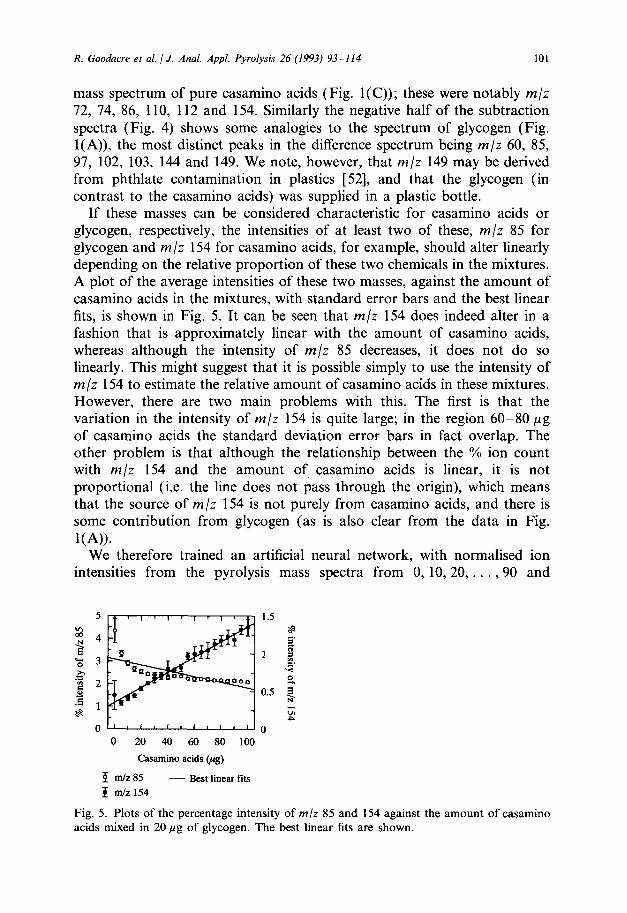
If these masses can be considered characteristic for casamino acids or glycogen, respectively, the intensities of at least two of these, m/z 85 for glycogen and m/z 154 for casamino acids, for example, should alter linearly depending on the relative proportion of these two chemicals in the mixtures. A plot of the average intensities of these two masses, against the amount of casamino acids in the mixtures, with standard error bars and the best linear fits, is shown in Fig. 5. It can be seen that m/z 154 does indeed alter in a fashion that is approximately linear with the amount of casamino acids, whereas although the intensity of m/z 85 decreases, it does not do so linearly. This might suggest that it is possible simply to use the intensity of m/z 154 to estimate the relative amount of casamino acids in these mixtures. However, there are two main problems with this. The first is that the variation in the intensity of m/z 154 is quite large; in the region 60-80 pg of casamino acids the standard deviation error bars in fact overlap. The other problem is that although the relationship between the % ion count with m/z 154 and the amount of casamino acids is linear, it is not proportional (i.e. the line does not pass through the origin), which means that the source of m/z 154 is not purely from casamino acids, and there is some contribution from glycogen (as is also clear from the data in Fig.

l(A)). We therefore trained an artificial neural network, with normalised ion

intensities from the pyrolysis mass spectra from 0, 10, 20, . . . ,90 and

5 1.5 z 8

2 4 P 5’ 8 % 3 B 1 E h

=a* 5

.Z 0 0 B 2 000 s 0.5 .E .

1 $

# E 0 0

0 20 40 60 80 100

Casamino acids (pg)

9 m/z 85 - Best linear fits

I m/z 154

Fig. 5. Plots of the percentage intensity of m/z 85 and 154 against the amount of casamino acids mixed in 20 pg of glycogen. The best linear fits are shown.

102 R. Goodacre et al. / J. Anal. Appl. Pyrolysis 26 (1993) 93-114

0.8

8 0.6 E

3 Oe4 0.2

II ,r,,,d 11111111 I

loo 10’ 102 l@ 10' 105

Number of epochs

Fig. 6. The learning curve(s) for the neural network using the standard back-propagation algorithm with one hidden layer consisting of eight nodes, trained with 0, 10, 20. . 90 and 100 fig of casamino acids.

100 pg of casamino acids in 20 pg of glycogen as inputs, and the stated amounts of casamino acids as outputs. We used the standard back-propagation algorithm, and the effectiveness of training was expressed in terms of the r.m.s. error between the actual and the desired outputs; this “learning curve” is shown in Fig. 6. Training was effected five times, using randomised, small initial values for the starting weights; because the five curves were superimposed, despite the randomised starting connection weights, it is clear that training was executed in a rather reproducible manner. It can be seen in the learning curve (Fig. 6) that the network very quickly reached a plateau (after about 100 epochs; r.m.s. error = 0.035-0.04) and training was nearly finished. When the network was trained further, the r.m.s. error had gradually decreased between 2-5 x lo4 epochs to a value between 0.01 and 0.005; at this level the r.m.s. error was observed to fluctuate between 0.005 and 0.01, and we considered training to have finished. At the end of training, when the r.m.s. error had reached approximately 0.01, the network was interrogated both with the pyrolysis-mass spectra that had been used to train the network (0, 10, 20, 30, 40, 50, 60, 70, 80, 90 and 100 pg casamino acids) and with “unknown” spectra (5, 15, 25, 35, 45, 55, 65, 75, 85 and 95 pg casamino acids) which were not in the training set. A plot of the network estimate vs. the true output (the amount of casamino acids) (Fig. 7(A)) gave a proportional fit (i.e. y = x), which was indistinguishable from the “expected” linear fit, and it was evident that the network estimate of the quantity of casamino acids in the mixtures was very similar to the true quantity, both for spectra that were used as the training set and for the “unknown” pyrolysis-mass spectra. Similar results were also found for the other three algorithms used (Fig. 7(A)), with similar r.m.s. error values being reached, and together they show that the combination of Py-MS and ANNs was able quantitatively to detect the amount of casamino acids in the range 0- 100 ,ug when they were mixed with 20 pg of glycogen.

R. Goodacre et al. / J. Anal. Appl. Pyrolysis 26 (1993) 93- 114 103

A 100

2 80

E .s 60

s 8 40

3

g 20

0

B loo

2 80

E -2 60

_* 3 40

2. z” 20

0

0 20 40 60 80

Casamino acids @g)

100

0 20 40 60 80

True numerical value

100

o Standard Back Propagation

n Stochastic Back Propagation

A Quick Propagation

v Weigend Weight Eliminator

- Expected linear fit

Fig. 7. Results of the estimates of trained neural networks against (A) true casamino acids concentration and (B) true numerical values, using a variety of (back-propagation) algorithms all running on the accelerator board with one hidden layer consisting of eight nodes. The training set consisted of either (A) 0, 10, 20 . . 90 and 100 mg/ml of casamino acids, or (B) the true numerical values from 0 to 100 in steps of 10. The expected linear fit is shown.

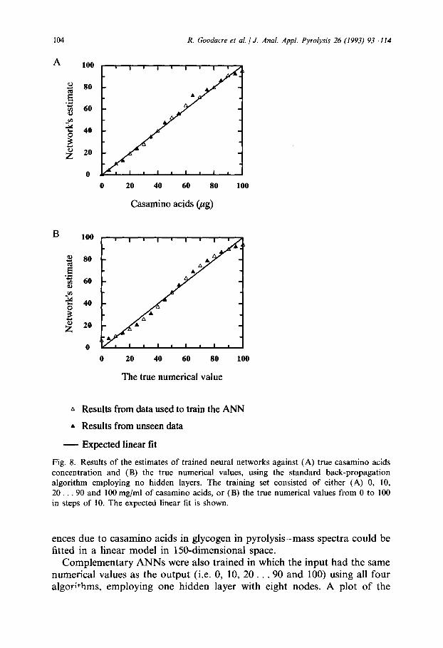
In other studies ANNs were set up using the standard back-propagation algorithm with the same architecture as the ones used above except that they contained no hidden layers. It was interesting to observe that the networks were still able to converge (Fig. 8(A)), indicating that the differ-


0 20 40 60 80 100

Casamino acids @g)

0 20 40 60 80 100

The true numerical value

n Results from data used to train the ANN

A Results from unseen data


Fig. 8. Results of the estimates of trained neural networks against (A) true casamino acids concentration and (B) the true numerical values, using the standard back-propagation algorithm employing no hidden layers. The training set consisted of either (A) 0, 10, 20 . . 90 and 100 mg/ml of casamino acids, or (B) the true numerical values from 0 to 100 in steps of 10. The expected linear fit is shown.

ences due to casamino acids in glycogen in pyrolysis-mass spectra could be fitted in a linear model in 150-dimensional space.

Complementary ANNs were also trained in which the input had the same numerical values as the output (i.e. 0, 10, 20 . . . 90 and 100) using all four algori+kms, employing one hidden layer with eight nodes. A plot of the

R. Goodacre et al. / J. Anal. Appl. Pyrolysis 26 (1993) 93 - I14 105

network estimate vs. the true output (Fig. 7(B)) also, as expected, gave a proportional fit for all the algorithms. The Weigend weight eliminator algorithm led, however, to a slightly sigmoidal plot; this might be because networks trained with this algorithm were not able to learn beyond an r.m.s. error of 0.04.

When ANNs were set up using the standard back-propagation algorithm with no hidden layers, which appeared to stop training at an r.m.s. error of 0.038, a plot of the network estimate vs. the true output (Fig. 8(B)) was not proportional but sigmoidal. This is likely to be a reflection of the sigmoidal squashing function f used to scale the signal passing through the output nodes.

In separate experiments (data not shown) ANNs were trained as above, employing only the standard back-propagation algorithm using one hidden layer with eight nodes, and the effectiveness of generalisation was estimated by calculating the standard error of regression for the network estimate vs. true output. It was found that the ANNs generalised after an r.m.s. error of between 0.02 and 0.03 was reached after 5-9 x lo3 epochs.

Since we have seen that it is possible to accurately determine the amount of one determinand in a mixture using the present approach, the question arises as to how many data points between 0 and 100 pg of casamino acids are needed to allow the network to generalise well? In order to elucidate this, several networks were run, using either the normalised pyrolysis-mass spectra or the true numerical values as the inputs. Plots of the network estimate vs. the true output are shown in Fig. 9. When the four pyrolysis- mass spectra from the samples containing 50 pg of casamino acids in glycogen were used to train the network, or when the input was only 50, the network, not surprisingly, was unable to generalise and all outputs were very close to 50 (Fig. 9(A)), i.e. very close to the only “knowledge” to which the network had been exposed. If the inputs used consisted of the values 0 and 100 only, the network again learnt the inputs which it had seen, but failed to generalise resulting in sigmoidal plots (Fig. 9(B)). Interestingly, the two sets of estimates are not superimposed; the network estimates from pyrolysis-mass spectral input approximates to 100 at much lower values of the abscissa than with the estimates from the true numerical data. Similarly shaped plots were observed (Fig. 9(C)) when 0, 50 and 100 were the inputs. In this instance what the network had seen (its training set) was very well estimated, but the unknown spectra or numerical inputs were badly estimated. When more data points are used (0, 35, 65 and 100; Fig. 9(D) and 0, 25, 50, 75 and 100; Fig. 9(E)), the network estimate began to become more like the true output, both for the training set and the unknown inputs, although there were still some sigmoidal deviations from the expected linear fit. In each case the pattern was clear; the network learnt its training set perfectly, but generalisation was less than perfect, at least until some ten equally spaced samples were used (Fig. 7).

106 R. Goodacre et al. 1 J. Anal. Appl. Pyrolysis 26 (1993) 93- 114

A loo

80

60

40

20

0

100

80

60

40

20

0

0 20 40 60 80 loo

Casamino acids (@g) or the true

numerical value

0 20 40 60 80 100

Casamino acids (pg) or the true

numerical value

0 20 40 60 so loo

Casamino acids @g) or the true numerical value

Fig. 9. (A-C)

R. Goodacre et al. / J. Anal. Appl. Pyrolysis 26 (1993) 93-l 14

0 20 40 60 80 100

Casamino acids @g) or the true

numerical value

107

0 20 40 60 So 100

Casamino acids @g) or the true numerical value

o Mixing casamino acids in glycogen - ANN training set

l Mixing casamino acids in glycogen - unseen spectra

q Results from numerical values - ANN training set

n Results from numerical values - unseen numbers


Fig. 9. Results of the estimates of trained neural networks against true casamino acid concentration (O-100 pg) ( 0) and the estimates against the true numerical values (o-100) ( l ), using the standard back-propagation with one hidden layer consisting of eight nodes running on the accelerator board. Various training sets were run: (A) 50 pg only; (B) 0 and 1OOpg; (C) 0, 50 and IOOpg; (D) 0, 35, 65 and 1OOpg; (E) 0, 25, 50, 75 and 100 pg of casamino acids or true numerical value. The expected linear fits are shown.

However, when’ using ten equally spaced samples as the training set, over the desired concentration range, even though the network estimate is linear, the edges of the data range were nearly always sigmoidal. Figure 10 demonstrates this more obviously, and shows the results obtained from

108 R. Goodacre et al. 1 J. Anal. Appl. Pyrolysis 26 (1993) 93-114

0 20 40 60 80 100


- Trained to an RMS error of 0.05

Trained to an RMS error of 0.01

- Trained to an RMS error of 0.001

Fig. 10. Results of the estimates of trained neural networks against the true numerical values, using standard back-propagation algorithm. The training set consisted of 0 to 100 in steps of 10 and the test set of 0 to 100 in steps of 1. Data points are joined by straight lines.

training an ANN on numerical input (0 to 100 in steps of 10) to an r.m.s. error of 0.05,O.Ol and 0.001, and interrogating with 0 to 100 in steps of unity. It is, therefore, always best to test near the middle of the concentration range because this will contain the most accurate part of the “calibration curve”.

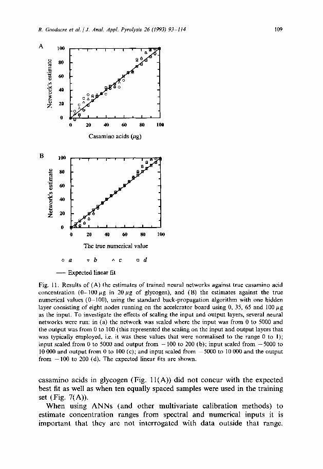
The effect of altering the scaling range in the input and output nodes of ANNs using 0, 35, 65 and 100 in the training set was investigated to determine whether this would improve the ability of the network to generalise. A variety of scaling ranges was employed. The first (a) represented the normally used scaling ranges of 0 to 5000 in the input layer and from 0 to 100 in the output layer. Other ANNs were also used: those where only the output was altered to scale between - 100 and 200 (b); those where only the input scale was altered to lie between - 5000 and 10 000 (c); those employing input and output nodes that were scaled between - 5000 and 10 000 and - 100 and 200 respectively (d).

After the ANNs were trained they were interrogated and the network estimates were plotted against the desired outputs, both for Py-MS data (Fig. 1 l(A)) and true numerical data (Fig. 1 l(B)). In Fig. 1 l(B) it is clear that scaling the input node (condition c) has no effect on improving the ability of the network to generalise. In contrast, however, when the output node was scaled from - 100 to 200 (in conditions b and d) the network estimate was very much like the desired output, and coincident with the expected best fit. There was also some improvement when the output was scaled ( - 100 to 200) when using pyrolysis-mass spectra as the training data. However, a plot of the network estimate vs. the actual amount of


0 20 40 60 80 loo

Casamino acids (pg)

0 20 40 60 80 loo


a v b A c ad

Expected linear fit

Fig. 11. Results of (A) the estimates of trained neural networks against true casamino acid concentration (O-100 pg in 20 pg of glycogen), and (B) the estimates against the true numerical values (O-100) using the standard back-propagation algorithm with one hidden layer consisting of eight nodes running on the accelerator board using 0, 35, 65 and 100 pg as the input. To investigate the effects of scaling the input and output layers, several neural networks were run: in (a) the network was scaled where the input was from 0 to 5000 and the output was from 0 to 100 (this represented the scaling on the input and output layers that was typically employed, i.e. it was these values that were normalised to the range 0 to 1); input scaled from 0 to 5000 and output from - 100 to 200 (b); input scaled from - 5000 to 10 000 and output from 0 to 100 (c); and input scaled from - 5000 to 10 000 and the output from - 100 to 200 (d). The expected linear fits are shown.

casamino acids in glycogen (Fig. 1 l(A)) did not concur with the expected best fit as well as when ten equally spaced samples were used in the training set (Fig. 7(A)).

When using ANNs (and other multivariate calibration methods) to estimate concentration ranges from spectral and numerical inputs it is important that they are not interrogated with data outside that range.

110

A 100

380

z % t3@ _- -ii 40

$ g 20

0

B 100

0 I 80

E '$ 60

_* 3 40

g p 20

0

R. Goodacre et al. 1 J. Anal. Appl. Pyrolysis 26 (1993) 93-114

0 20 40 60 80 100


numerical value

0 20 40 60 80 100


numerical value

o Mixing casamino acids in glycogen - ANN training set

l Mixing casamino acids in glycogen - unseen spectra

q Results from numerical values - ANN training set

l Results from numerical values - unseen numbers


Fig. 12. Results of the estimates of trained neural networks against true casamino acid concentration (O-100 pg in 20 pg of glycogen) (0, 0) and the estimates against the true numerical values (o-100) ( n , q ), using the standard back-propagation algorithm with one hidden layer consisting of eight nodes running on the accelerator board using (A) 0, 25-75 (in steps of 5 pg) and 100 pg, or (B) only 25-75 (in steps of 5 pg), in the training set.

Figure 12(A) shows the network estimates against true values using an input of 0, 25 to 75 (in steps of 5) and 100 pg of casamino acids, and the true numerical values. ANNs were also trained on the same two training sets, except that data for 0 and 100 values were omitted (Fig. 12(B)). When Figs. 12(A) and 12(B) are compared, the former shows a more linear relationship

R. Goodacre et al. 1 J. Anal. Appl. Pyrolysis 26 (1993) 93-114

A 100

2 80

f + 60

s $ 40

5 g 20

0

0 20 40 60 80

Casamino acids @g)

100

0 20 40 60 80 loo


a v b fi c q d

Expected linear fit

Fig. 13. The effect of training neural networks with 25 -75 pg (in steps of 5 pg) using (A) true casamino acid concentrations (O-100 pg in 20 pg of glycogen), and (B) true numerical values (0- 100) employing the standard back-propagation algorithm with one hidden layer consisting of eight nodes running on the accelerator board. Results are expressed as (A) the estimates of the trained neural networks vs. the true casamino acids concentration, and (B) the estimates against the true numerical values. The effects of scaling the input and output layers of the neural networks are shown. (For details of scaling see Fig. 11.) The expected linear fits are shown.

at the edges of the data ranges and the edges of the latter plot are much more sigmoidal.

The effect of altering the scaling range in the input and output nodes was also investigated for both PJ-MS (Fig. 13(A)) and true numerical data (Fig. 13(B)) containing only values from 25 to 75 (in steps of 5) in the training set. ANNs were set up under the four conditions (a-d) outlined above. The ability of the network to generalise was improved slightly by scaling the output, but was not as obvious as that reported above (Fig. 1 l), both for Py-MS (Fig. 13(A)) and for true numerical data (Fig. 13(B)).

112 R. Goodacre et al. / J. Anal. Appl. Pyrolysis 26 (1993) 93-l I4

Indeed, when the input layer alone was scaled between - 5000 and 10 000 (condition c) for pyrolysis-mass spectra as the input (Fig. 13(A)), the network estimates of what it had not seen were worse than the normally used conditions of scaling the input from 0 to 5000 and the output from 0 to 100 (a). It is also interesting to note that scaling only the output layer (condition b) of ANNs trained using Py-MS data caused their learning curves to be smoother (data not shown) than those using the normal scaling ranges (a).

These results demonstrate that neither ANNs of the present type nor data derived from the Py-MS of complex mixtures can be expected to give good extrapolations from linear numerical data (the true numbers).

In summary, we have shown that the combination of Py-MS and ANNs was able to quantitatively deconvolute the Py-MS of mixtures of casamino acids in glycogen, and that a training set of ten equally spaced samples over the desired concentration range should be used in the network training set if accurate quantitative values are required. Further, ANNs should not be expected to give wholly correct estimates near the edges of or outside their training sets. We conclude that the combination of Py-MS and ANNs constitutes a novel, powerful and interesting technology for the analysis of the concentrations of appropriate substrates, metabolites and products in biochemical processes generally. Future work will involve assessing the use of a linear activation function to ascertain if it may improve the ability of ANNs to generalise from pyrolysis-mass spectral data.

ACKNOWLEDGEMENTS

This work is supported by the Biotechnology Directorate of the UK SERC LINK scheme in Biochemical Engineering, in collaboration with Horizon Instruments, ICI Biological Products and Fine Chemicals, and Neural Computer Sciences.

REFERENCES

1 D.B. Drucker, Meth. Microbial., 9 (1976) 51-125. 2 W.J. Irwin, Analytical Pyrolysis: A Comprehensive Guide, Marcel Dekker, New York, 1982. 3 H.L.C. Meuzelaar, J. Haverkamp and F.D. Hileman, Pyrolysis Mass Spectrometry of

Recent and Fossil Biomaterials, Elsevier, Amsterdam, 1982. 4 C.S. Gutteridge, Methods Microbial., 19 (1987) 227-272. 5 R.C.W. Berkeley, R. Goodacre, R.J. Helyer and T. Kelley, Lab. Pratt., 39 (1990) 81-83. 6 L.A. Shute, C.S. Gutteridge, J.R. Norris and R.C.W. Berkeley, J. Gen. Microbial., 130

(1984) 343-355. 7 G. Wieten, H.L.C. Meuzelaar and K. Haverkamp, in G. Odham, L. Larsson and P-A.

Mardh (Eds.), Gas Chromatography/Mass Spectrometry: Applications in Microbiology, Plenum Press, New York, 1984, pp. 335-380.

8 R. Goodacre and R.C.W. Berkeley, FEMS Microbial. Lett., 71 (1990) 133-138.


9

10 11

12

13

14

15

16

17

18

19

20 21

22

23 24 25

26 27

28 29

30 31

32

33 34

35

36

37 38

R. Goodacre, J.E. Beringer and R.C.W. Berkeley, J. Anal. Appl. Pyrolysis, 22 (1991) 19-28. R. Kajioka and P.W. Tang, J. Anal. Appl. Pyrolysis, 6 (1984) 59-68. P.R. Sisson, R. Freeman, N.F. Lightfoot and I.R. Richardson, Epidemiol. Infect., 107 (1991) 127-132. H.L.C. Meuzelaar, P.G., Kistemaker, W. Eshuis and H.W.B. Engel, Rapid Methods and Automation in Microbiology, Learned Information, Oxford, 1976, pp. 225-230. G. Wieten, K. Haverkamp, H.B.W. Engel and L.G. Berwald, Rev. Infect. Diseases, 3 (1981) 871-877. G. Wieten, K. Haverkamp, H.L.C. Meuzelaar, H.B.W. Engel and L.G. Berwald, J. Gen. Microbial., 122 (1981) 109-l 18. R. Freeman, M. Goodfellow, F.K. Gould, S.J. Hudson and N.F. Lightfoot, J. Med. Microbial., 32 (1990) 283-286. R. Freeman, F.K. Gould, R. Wilkinson, A.C. Ward, N.F. Lightfoot and P.R. Sisson, Epidemiol. Infect., 106 (1991) 239-246. F.K. Gould, R. Freeman, P.R. Sisson, B.D. Cookson and N.F. Lightfoot, J. Hosp. Infect., 19 (1991) 41-48. J.T. Magee, J.M. Hindmarch, L.A. Burnett and A. Pease, J. Med. Microbial., 30 (1989) 273-278. R. Freeman, F.K. Gould, P.R. Sisson and N.F. Lightfoot, Lett. Appl. Microbial., 13 (1991) 28-31. W. Windig and H.L.C. Meuzelaar, Anal. Chem., 56 (1984) 2297-2303. N.H. Nie, C.H.G. Hull, J.G. Jenkins, K. Steinbrenner and W.H. Brent, Statistical Package for the Social Sciences, McGraw-Hill, New York, 1975. W. Windig, P.G. Kistemaker and J. Haverkamp, J. Anal. Appl. Pyrolysis, 3 (1981) 199-212. R. Goodacre and D.B. Kell, Anal. Chim. Acta, (1993) in press. R. Goodacre, D.B. Kell and G. Bianchi, Nature, 359 (1992) 594. D.L. Massart, B.G.M. Vandeginste, S.N. Deming, Y. Michotte and L. Kaufmann, Chemometrics: A textbook, Elsevier, Amsterdam, 1988. H. Martens and T. Naes, Multivariate Calibration, Wiley, New York, 1989. R.G. Brereton, Chemometrics: Applications of Mathematics and Statistics to Laboratory Systems, Ellis Horwood, New York, 1990. S.D. Brown, Anal. Chem., 64 (1992) 22R-49R. D.E. Rumelhart, J.L. McClelland and the PDP Research Group, Parallel Distributed Processing. Experiments in the Microstructure of Cognition, Vols. I & II, MIT Press, Cambridge, MA, 1986. J.D. Cowan and D.H. Sharp, Q. Rev. Biophys., 21 (1988) 365-427. J.L. McClelland and D.E. Rumelhart, Exploration in Parallel Distributed Processing; A Handbook of Models, Programs and Exercises, MIT Press, Cambridge, MA, 1988. D.J. Amit, Modeling Brain Function; the World of Attractor Neural Networks, Cam- bridge University Press, UK, 1989. T. Kohonen, Self-Organization and Associative Memory, Springer, Heidelberg, 1989. P.D. Wasserman, Neural Computing: Theory and Practice, Van Nostrand Reinhold, New York, 1989. P.D. Wasserman and R.M. Oetzel, NeuralSource: the Bibliographic Guide to Artificial Neural Networks, Van Nostrand Reinhold, New York, 1989. I. Aleksander and H. Morton, An Introduction to Neural Computing, Chapman & Hall, London, 1990. R. Beale and T. Jackson, Neural Computing: An Introduction, Adam Hilger, Bristol, 1990. R.C. Eberhart and R.W. Dobbins, Neural Network PC Tools, Academic Press, London, 1990.


39 Y-H. Pao, Adaptive Pattern Recognition and Neural Networks, Addison-Wesley, Read- ing, MA, 1989.

40 P.K. Simpson, Artificial Neural Systems, Pergamon, Oxford, 1990. 41 J. Hertz, A. Krogh and R.G. Palmer, Introduction to the Theory of Neural Computa-

tion, Addison-Wesley, Redwood City, 1991. 42 K. Hornik, M. Stinchcombe and H. White, Neural Networks, 2 (1989) 359-368. 43 K. Hornik, M. Stinchcombe and H. White, Neural Networks, 3 (1990) 551-560. 44 H. White, Neural Networks, 3 (1990) 535-549. 45 B. Curry and D.E. Rumelhart, MSnet: A Neural Network that Classifies Mass Spectra,

Hewlett Packard technical report HPL-90- 16 1, 1990. 46 R.E. Aries, C.S. Gutteridge and T.W. Ottley, J. Anal. Appl. Pyrolysis, 9 (1986) 81-98. 47 P.J. Werbos, Masters thesis, Harvard University, Boston, MA, 1974. 48 D. Ackley, G. Hinton and T. Sejnowski, Cognitive Sci., 9 (1985) 147-169. 49 H. Szu, in J. Denker (Ed.), AIP Conference Proceedings 151: Neural Networks for

Computing, American Institute of Physics, New York, 1986, pp. 420-425. 50 SE. Fahlman, An empirical study of learning speed in back propagation networks,

Technical report, Carnegie-Mellon University, Pittsburgh, PA, 1988. 51 AS. Weigend, D.E. Rumelhart and B.A. Huberman, in R.P. Lippmann, J.E. Moody and

D.S. Touretzky (Eds.), Neural Information Processing Systems 3, Morgan Kaufmann, San Mateo, CA, 1991, pp. 875-882.

52 B.S. Middleditch, Analytical Artifacts, Elsevier, Amsterdam, 1989.

Quantitative analysis of the pyrolysis-mass ... - DBK...

Documents

Transcript of Quantitative analysis of the pyrolysis-mass ... - DBK...