Rapid Response Energy Brief

February 2015 3 3

The INSIGHT_E project is funded by the European Commission under the 7th Framework Program for Research and Technological Development (2007-2013).

This publication reflects only the views of its authors, and the European Commission cannot be held responsible for its content.

1

Quantifying the "merit-order" effect in

European electricity markets Lead author: Paul Deane (UCC)

Authoring team: Seán Collins, Brian Ó Gallachóir (UCC), Cherrelle Eid (IFRI), Rupert Hartel, Dogan Keles,

Wolf Fichtner (KIT).

Reviewer: Alberto Ceña (Kic)

Legal Notice: Responsibility for the information and views set out in this paper lies entirely with the authors.

Introduction

The electricity production from renewable energy sources (RES) has increased in most European member states over the past 10-15 years. The investment incentive for RES is mainly driven by

policy support measures such as feed-in tariffs, which guarantee a fixed price per unit of renewable electricity generated, while other generators must sell their electricity in a spot market. However, the influence of RES on electricity spot market prices is growing with the increasing share of renewable electricity deployed. This is due to the how spot

prices are determined as a function of supply and demand. The supply curve, the so called merit order, is derived by ordering the supplier bids

according to ascending marginal cost. The intersection of the demand curve with the merit-order defines the market clearing price i.e. the electricity spot market price. The feed-in of

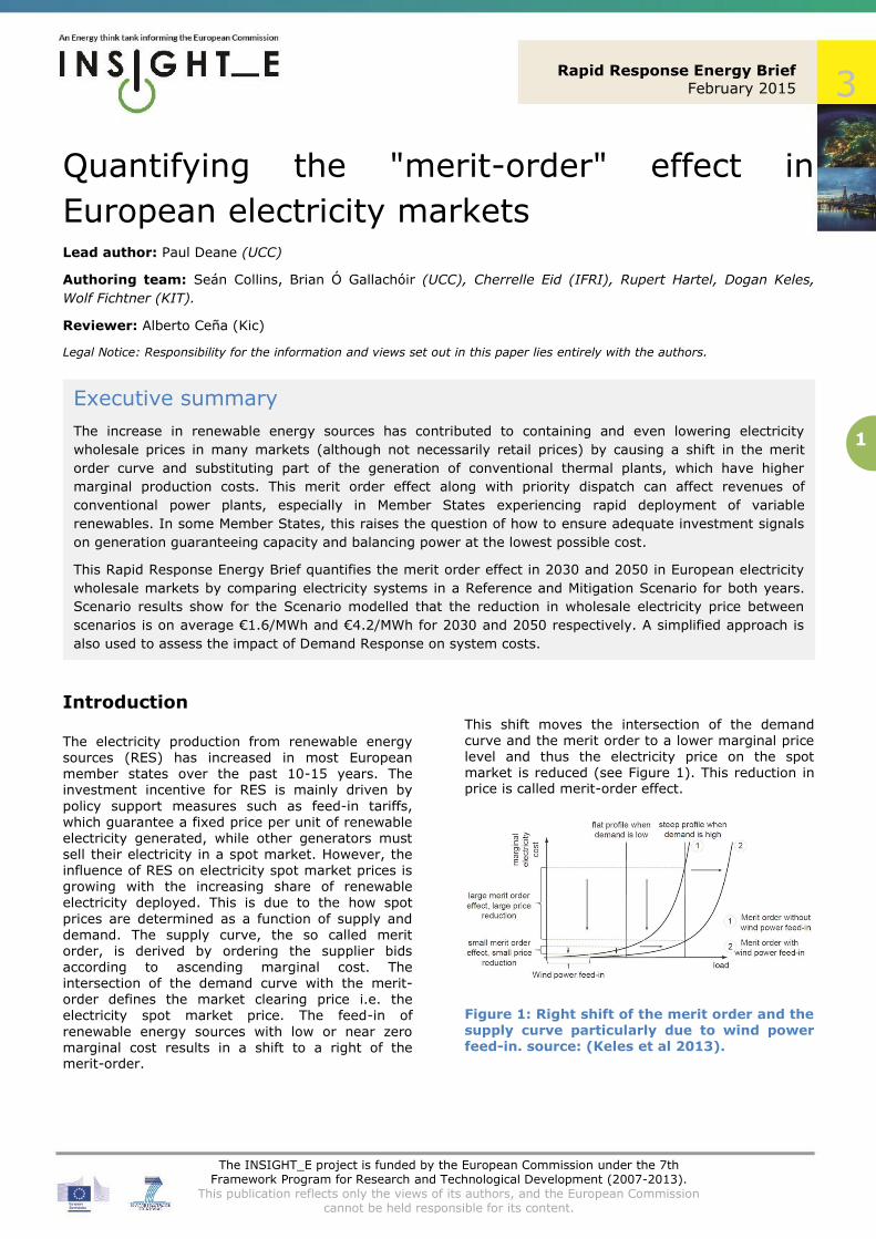
renewable energy sources with low or near zero marginal cost results in a shift to a right of the merit-order.

This shift moves the intersection of the demand curve and the merit order to a lower marginal price level and thus the electricity price on the spot market is reduced (see Figure 1). This reduction in price is called merit-order effect.

Figure 1: Right shift of the merit order and the supply curve particularly due to wind power feed-in. source: (Keles et al 2013).

Executive summary

The increase in renewable energy sources has contributed to containing and even lowering electricity

wholesale prices in many markets (although not necessarily retail prices) by causing a shift in the merit

order curve and substituting part of the generation of conventional thermal plants, which have higher

marginal production costs. This merit order effect along with priority dispatch can affect revenues of

conventional power plants, especially in Member States experiencing rapid deployment of variable

renewables. In some Member States, this raises the question of how to ensure adequate investment signals

on generation guaranteeing capacity and balancing power at the lowest possible cost.

This Rapid Response Energy Brief quantifies the merit order effect in 2030 and 2050 in European electricity

wholesale markets by comparing electricity systems in a Reference and Mitigation Scenario for both years.

Scenario results show for the Scenario modelled that the reduction in wholesale electricity price between

scenarios is on average €1.6/MWh and €4.2/MWh for 2030 and 2050 respectively. A simplified approach is

also used to assess the impact of Demand Response on system costs.

.

Rapid response Energy Brief

February 2015 3

2

This RREB provides a brief review of ex-post

analyses carried out on the merit order effect and then looks ahead to 2030 and 2050, carrying out an ex ante analysis of the merit order effect of the energy scenarios EU 2030 Climate and Energy

Policy Framework1. Note that it is not the objective

of this RREB to undertake a qualitative analysis of the technical appropriateness of the portfolios or results from the 2030 EU Policy Framework. Results will specifically focus on the merit order effect.

Review of ex post analyses of the

merit order effect

There is a significant amount of analysis of the merit order effect, the bulk of which are referred to in (Azofra et al., 2014) and (Ray 2010). These

studies can in general be categorised as model based or statistical based studies.

We present here a statistical analysis of the merit-order effect using the example of wind power in Germany. The merit-order effect can be shown by analysing historical market prices from the European Electricity Exchange (EEX). According to (Keles et al 2013), linear regression of market prices and wind power feed-in points to an average

price reduction of €1.47/MWh for every additional GW of wind power. This average effect cannot explain extreme price events. “Thus, the correlation of electricity price and wind power feed-in might depend on point of time and is presumably nonlinear” according to (Keles et al 2013). To

further analyse the price reduction effect the

current power plant mix as well as the demand situation are taken into account. Therefore an hourly record of electricity price, wind power feed-in and demand (load) is formed and sorted ascending by the load. With a linear regression the price change αL as a function of the load can be

shown in Figure 2. The negative values indicate that the wind power feed-in leads to lower electricity prices. Furthermore, it can be obtained that the price reduction effect highly depends on the load situation and can be significantly higher than the average reduction of 1.47 €/MWh (see Figure 2). This is in line with the findings of (Hirth 2013).

(Hirth 2013) further shows that this price reduction also affects the market value of variable renewables and is also dependent on the penetration of renewable energies. The market value of wind

power falls from 110 % of the average power price to 50-80 % with an increase of wind power penetration from zero to 30% of total electricity production (Hirth 2013).

1 http://ec.europa.eu/clima/policies/2030/index_en.htm

Figure 2: Average change of the deseasonalized electricity price per GW wind power depending on load interval (Keles et al 2013).

A further comparison of price reductions in the

German merit order curve is shown in Figure 3. There are four significant changes in the curve according to (Keles et al 2013). These changes can in general be linked to technology switches in the merit order. In area ‘I’, a local peak is evident, representing the change from lignite to coal fired

power plants. The price reduction effect increases when lignite fired power plants are the price setting units instead of coal. A similar peak can be obtained in area ‘III’ where a switch from coal to gas fired power plants occurs in the merit order, although the price reduction effect in area ‘I’ is higher than in area ‘III’. The occurrence of negative prices is high

in this area because plant operators try to avoid shut-down and ramp-up costs and accept negative electricity prices to stay online. Other restrictions like reserve requirements and, in the case of gas

fired power plants, heat delivery, cause plant operators to be online which can lead to an excess electricity supply and thus to negative prices. Area

IV represents the peak load power plants (oil or gas fired) which are the most expensive power plants due to their low efficiency and high fuel costs. In this area the price reduction effect is very high, if their utilisation is avoided.

30 35 40 45 50 55 60 65 70 75 80-10

-8

-6

-4

-2

0

Load [GW]

Avera

ge c

hange in

ele

ctr

icity

price

[€/M

Wh] per

GW

of w

ind p

ow

er

feed-in

Price change L dependent on load

Average price change

Rapid response Energy Brief

February 2015 3

3

Figure 3: Price reduction per GW wind power feed-in depending on the load level and the German merit-order curve (Keles et al 2013).

The merit order effect outlined here is dependent on the German market design. However, other market designs would lead to a similar merit order effect according to (Keles et al 2013).

Traditionally, electricity demand does not respond to price levels changes that occur on spot or balancing markets. The traditional perspective of ”generation follows the demand” is however expected to change in a situation where the

demand responds to electricity price levels and consumers are able to benefit financially from shifting consumption.

Demand response (DR) is regarded as the modification of electricity consumption in response to price of electricity generation and state of the electricity system reliability (DOE, 2006). The communication of price levels to electricity consumers could lead to an electricity system

where increasingly the ”demand follows generation”. Within Europe, there are some standing arrangements to involve energy intensive industrial customers in DR. This is mostly done through critical peak pricing or time of use pricing and some system operators make use of large

avoided loads as part of their system balancing services (Torriti, Hassan, & Leach, 2010). However, this is still not applied in many European countries; DR is only commercially active as a

flexibility resource in France, Ireland, the United Kingdom, Belgium, Switzerland and Finland (SEDC, 2014). Countries with large penetration of RES such

as Germany currently use demand flexibility to maintain system-wide reliability (Koliou, Eid, Chaves-Ávila, & Hakvoort, 2014).

Demand response could reduce the required capacity of peaking electricity units, could increase

load factors of existing generation units and

furthermore can have positive effects on electricity network capacity utilization. Furthermore, demand response could be used to provide balancing capacity to complement the variability of renewable sources.

Demand response is anticipated to play a role in Europe in order to reach the 2020 targets and beyond. In particular, the Energy Efficiency Directive (EED), art. 15, explicitly urges EU national

regulatory authorities to encourage demand-side resources, including demand response, “to participate alongside supply in wholesale and retail markets”, and also to provide balancing and ancillary services to network operators in a non-discriminatory manner (EC, 2012). The European Commission states that the potential in Europe for

DR in electricity markets is believed to be high but is currently still underutilized (EC, 2013) due to the concentration on industrial users primarily. Residential users are in the future also expected to become involved in demand response provision but still some technical, regulatory and economic barriers exist (SEDC, 2014). In this RREB the

impact of DR on total system costs is quantified at an EU wide level in 2030 and 2050.

Ex-Ante Analysis of Merit Order Effect - Methodology

Looking ahead, we analyse the merit order effect in two distinct power plant portfolios in each of two

specific years (2030 and 2050) using a power

systems modelling model based approach. These portfolios are developed based on scenario analysis results carried out with the PRIMES model that were used to inform the EU 2030 Framework for climate and energy policies. The first scenario is a

Reference Scenario and the second scenario is a Mitigation Scenario. The merit order in this analysis is defined as the difference in price between the two scenarios. A brief description of the scenarios is provided here.

The Reference Scenario is the EU Reference Scenario2 2013 which explores the consequences of current trends including full implementation of policies adopted by late spring 2012. The Reference

scenario has been developed through modelling with PRIMES, GAINS and other related models and

benefited from the comments of Member States experts. The Reference scenario provides an energy system pathway up to 2050 affected by already agreed policies. The Mitigation Scenario by contrast, also provides an energy system pathway

up to 2050 but in this case achieves GHG

2 ec.europa.eu/smart-regulation/.../ia...2014/swd_2014_0015_en.pdf

Rapid response Energy Brief

February 2015 3

4

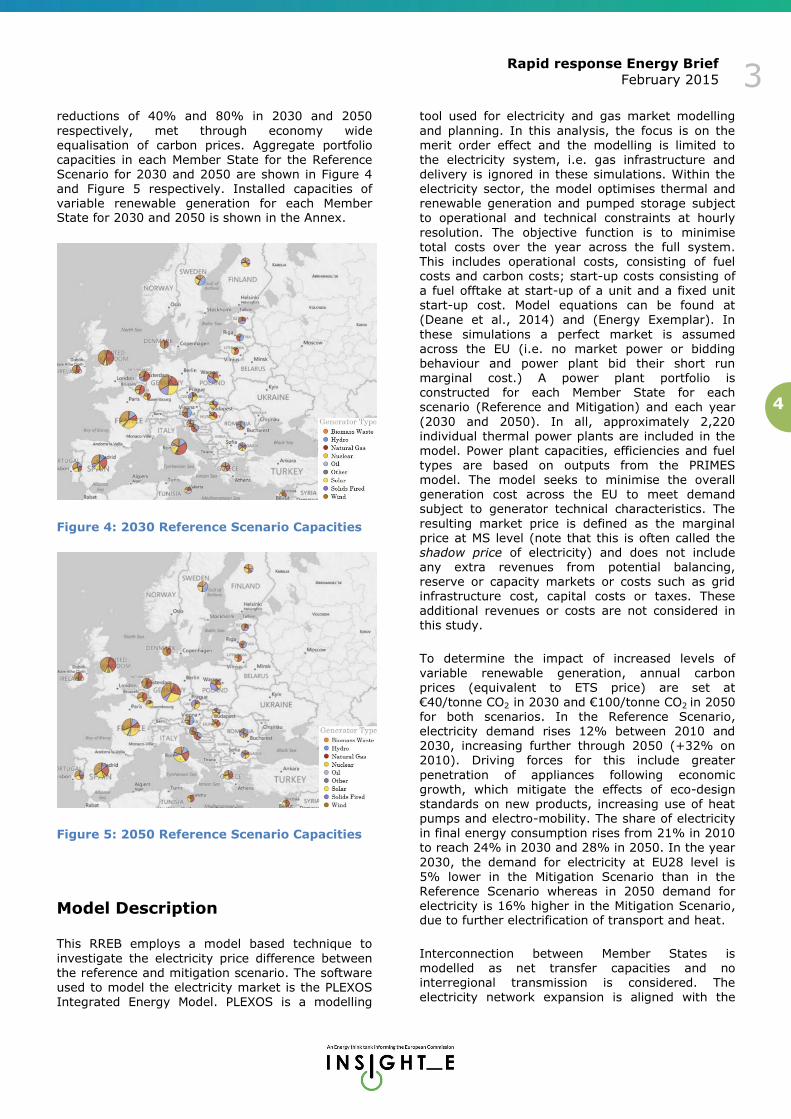
reductions of 40% and 80% in 2030 and 2050

respectively, met through economy wide equalisation of carbon prices. Aggregate portfolio capacities in each Member State for the Reference Scenario for 2030 and 2050 are shown in Figure 4 and Figure 5 respectively. Installed capacities of variable renewable generation for each Member State for 2030 and 2050 is shown in the Annex.

Figure 4: 2030 Reference Scenario Capacities

Figure 5: 2050 Reference Scenario Capacities

Model Description

This RREB employs a model based technique to

investigate the electricity price difference between the reference and mitigation scenario. The software used to model the electricity market is the PLEXOS Integrated Energy Model. PLEXOS is a modelling

tool used for electricity and gas market modelling

and planning. In this analysis, the focus is on the merit order effect and the modelling is limited to the electricity system, i.e. gas infrastructure and delivery is ignored in these simulations. Within the electricity sector, the model optimises thermal and renewable generation and pumped storage subject to operational and technical constraints at hourly

resolution. The objective function is to minimise total costs over the year across the full system. This includes operational costs, consisting of fuel costs and carbon costs; start-up costs consisting of a fuel offtake at start-up of a unit and a fixed unit start-up cost. Model equations can be found at (Deane et al., 2014) and (Energy Exemplar). In

these simulations a perfect market is assumed across the EU (i.e. no market power or bidding behaviour and power plant bid their short run

marginal cost.) A power plant portfolio is constructed for each Member State for each scenario (Reference and Mitigation) and each year

(2030 and 2050). In all, approximately 2,220 individual thermal power plants are included in the model. Power plant capacities, efficiencies and fuel types are based on outputs from the PRIMES model. The model seeks to minimise the overall generation cost across the EU to meet demand subject to generator technical characteristics. The

resulting market price is defined as the marginal price at MS level (note that this is often called the shadow price of electricity) and does not include any extra revenues from potential balancing, reserve or capacity markets or costs such as grid infrastructure cost, capital costs or taxes. These additional revenues or costs are not considered in

this study.

To determine the impact of increased levels of

variable renewable generation, annual carbon prices (equivalent to ETS price) are set at €40/tonne CO2 in 2030 and €100/tonne CO2 in 2050 for both scenarios. In the Reference Scenario, electricity demand rises 12% between 2010 and 2030, increasing further through 2050 (+32% on 2010). Driving forces for this include greater

penetration of appliances following economic growth, which mitigate the effects of eco-design standards on new products, increasing use of heat pumps and electro-mobility. The share of electricity in final energy consumption rises from 21% in 2010 to reach 24% in 2030 and 28% in 2050. In the year

2030, the demand for electricity at EU28 level is

5% lower in the Mitigation Scenario than in the Reference Scenario whereas in 2050 demand for electricity is 16% higher in the Mitigation Scenario, due to further electrification of transport and heat.

Interconnection between Member States is modelled as net transfer capacities and no interregional transmission is considered. The electricity network expansion is aligned with the

Rapid response Energy Brief

February 2015 3

5

latest 10 Year Development Plan from ENTSO-E,

without making any judgement on the likelihood of certain projects materialising. Fuel prices are also consistent across scenarios for each year and are shown in the Table 1.

Table 1: Fuel prices used in study1

Fuel prices 2030 2050

Oil (in €2010 per boe) 93 110

Gas (in €2010 per boe) 65 63

Coal (in €2010 per boe) 24 31

Results for 2030

Results for the year 2030 for each Member State are show in Figure 6 in terms of the absolute reduction in annual wholesale electricity price in the Mitigation scenario relative to the Reference

scenario. The absolute annual values are provided in the Annex. Results are driven by differences between the Reference and Mitigation Scenario portfolios and also by differences in demand. It can be seen the reduction in market price in the majority of central European Member States is relatively benign at less than €1.5/MWh with an

overall average of €1.6/MWh. The greatest impact is seen in the UK and Ireland. In the UK two elements are driving a strong reduction in wholesale price between the Reference and Mitigation Scenario. Firstly the demand in the

Mitigation Scenario is approximately 5% lower than

the Reference Scenario. Secondly there is a strong increase in installed renewable capacity with almost a third of the EU total offshore wind capacity installed in the UK. This has a strong seasonal impact and tends to reduce prices in the winter months when wind speeds are high and demand is also highest. This reduces the need for higher

marginal cost generators to meet peak demand. Similarly Ireland sees a strong reduction in price between the two scenarios and this is primarily driven by an increase in onshore wind capacity. Across the EU there is a general trend in the increase on variable renewable generation in the Mitigation Scenario and the drop in Market prices.

In contrast to the UK, Italy sees a large increase in PV and this has a big impact on wholesale

electricity prices in summer months with negligible differences in prices in winter. Results for The Netherlands show a 4% drop in wholesale market price between the Reference and Mitigation

Scenario driven in part by a drop in demand of almost 9% and an increases in both onshore and offshore wind energy. In the Baltic region, an increase in Biomass Waste fired generation capacity in Latvia and Lithuania coupled with an increase in

onshore wind capacity in Estonia contribute to

average price reductions of 3-4%.

Figure 6: Reduction in price (€/MWh) between Reference and Mitigation Scenario for 2030

On the Iberian Peninsula, both Spain and Portugal

have already high levels of renewables in the Reference Scenario. Demand drops by approximately 6% in both Member States for the

Mitigation Scenario. In the Mitigation Scenario Portugal has a reduced installed capacity of wind and solar energy and both Member States

experience only a minor reduction in prices. France is the Member States with the largest absolute reduction in demand. France also sees a strong increase in biomass waste capacity and associated generation in the mitigation scenario.

Rapid response Energy Brief

February 2015 3

6

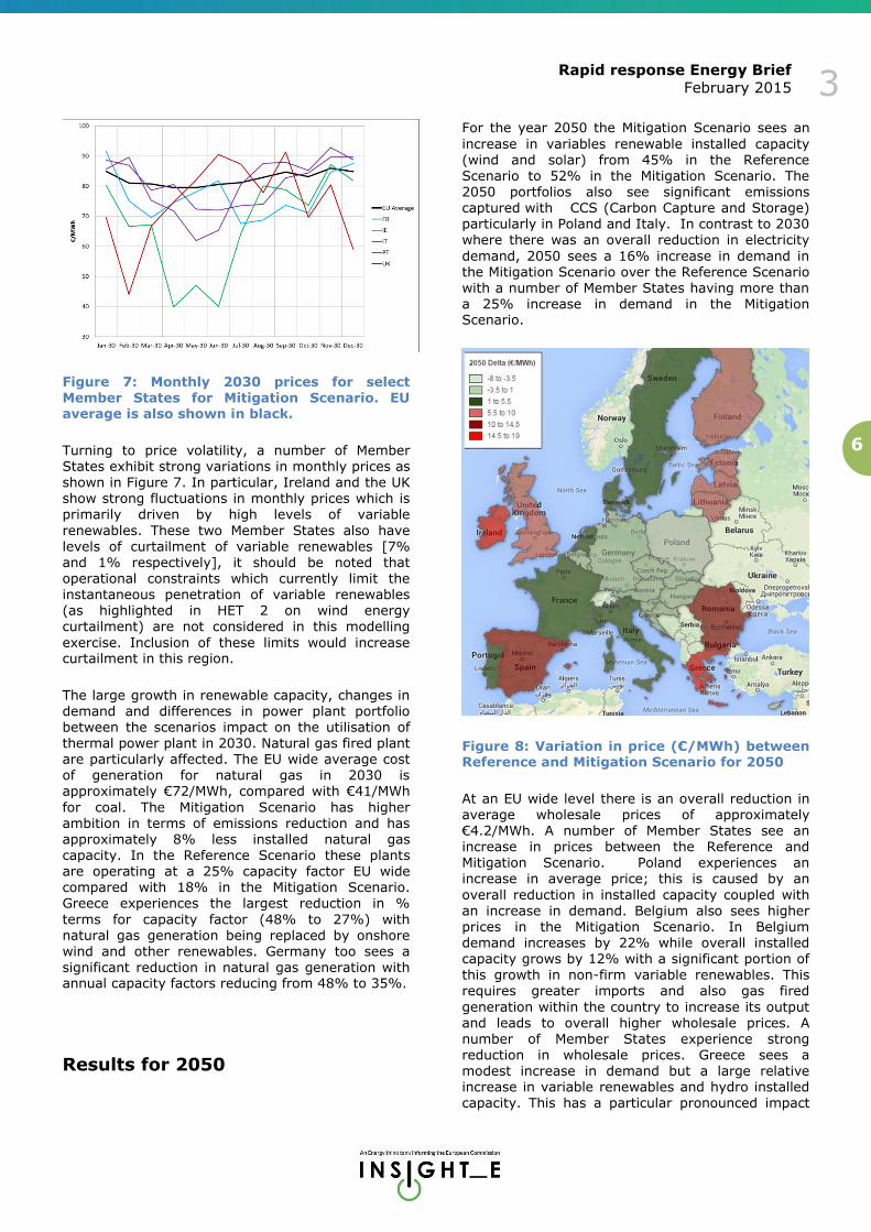
Figure 7: Monthly 2030 prices for select Member States for Mitigation Scenario. EU average is also shown in black.

Turning to price volatility, a number of Member States exhibit strong variations in monthly prices as shown in Figure 7. In particular, Ireland and the UK show strong fluctuations in monthly prices which is primarily driven by high levels of variable

renewables. These two Member States also have levels of curtailment of variable renewables [7% and 1% respectively], it should be noted that operational constraints which currently limit the instantaneous penetration of variable renewables (as highlighted in HET 2 on wind energy curtailment) are not considered in this modelling

exercise. Inclusion of these limits would increase curtailment in this region.

The large growth in renewable capacity, changes in demand and differences in power plant portfolio between the scenarios impact on the utilisation of thermal power plant in 2030. Natural gas fired plant are particularly affected. The EU wide average cost of generation for natural gas in 2030 is approximately €72/MWh, compared with €41/MWh

for coal. The Mitigation Scenario has higher ambition in terms of emissions reduction and has approximately 8% less installed natural gas capacity. In the Reference Scenario these plants are operating at a 25% capacity factor EU wide compared with 18% in the Mitigation Scenario. Greece experiences the largest reduction in %

terms for capacity factor (48% to 27%) with natural gas generation being replaced by onshore wind and other renewables. Germany too sees a

significant reduction in natural gas generation with annual capacity factors reducing from 48% to 35%.

Results for 2050

For the year 2050 the Mitigation Scenario sees an

increase in variables renewable installed capacity (wind and solar) from 45% in the Reference Scenario to 52% in the Mitigation Scenario. The 2050 portfolios also see significant emissions captured with CCS (Carbon Capture and Storage) particularly in Poland and Italy. In contrast to 2030 where there was an overall reduction in electricity

demand, 2050 sees a 16% increase in demand in the Mitigation Scenario over the Reference Scenario with a number of Member States having more than a 25% increase in demand in the Mitigation Scenario.

Figure 8: Variation in price (€/MWh) between Reference and Mitigation Scenario for 2050

At an EU wide level there is an overall reduction in average wholesale prices of approximately €4.2/MWh. A number of Member States see an increase in prices between the Reference and Mitigation Scenario. Poland experiences an increase in average price; this is caused by an

overall reduction in installed capacity coupled with an increase in demand. Belgium also sees higher prices in the Mitigation Scenario. In Belgium demand increases by 22% while overall installed capacity grows by 12% with a significant portion of

this growth in non-firm variable renewables. This requires greater imports and also gas fired

generation within the country to increase its output and leads to overall higher wholesale prices. A number of Member States experience strong reduction in wholesale prices. Greece sees a modest increase in demand but a large relative increase in variable renewables and hydro installed capacity. This has a particular pronounced impact

Rapid response Energy Brief

February 2015 3

7

especially in summer months when solar generation

is high. Elsewhere across the EU, the increase in installed capacity of variable renewable generation has strong implication for wholesale prices however addition of low carbon plant such as nuclear also has important implications. Romania has increased installed capacity of nuclear in the Mitigation Scenario and coupled with increase in variable

renewable generation contributes to a strong reduction in price.

It is important to remember also that the carbon price for the Mitigation Scenario is held at €100/t. In the EU Impact Assessment Document the Carbon price in the Mitigation Scenario is estimated at €264/t. This carbon price would lead to significantly higher prices in the Mitigation Scenario for all Member States.

Impact of demand response

Demand response can have a significant impact on the merit order. In this study the main type of

demand response that is considered is load shifting, meaning that the electricity demand has been shifted from peaking moments to off-peaking moments in time. To examine the impact of Demand Response (DR) simulations were undertaken for the Reference Scenarios where 10% and 15% of each Member State peak demand was

made available for demand response in 2030 and in 2050 respectively. Replacing this peak demand in

off-peak moments leaves the electricity demand equal for each year. Demand response consequently reduces the need for expensive peaking plants to operate and decreases the

marginal price while it increases load factors of the baseload units. Demand Response units are modelled as virtual pumped storage units with 100% efficiency. The optimiser’s objective function is to minimise total system costs whereas a customer using DR will aim to reduce their overall electricity bill. This is a relatively simple method to

simulate demand response and will not reflect full system benefits as it does not directly include a price response component (which is important with high levels of variable renewable generation) but provides a useful starting point in gauging its impact from a system wide perspective.

From an EU wide perspective, the introduction of DR in 2030 reduces total system generations costs (i.e. variable cost of generation and start-up costs

of generators) by €2.0bn or approximately €0.5/MWh. For the year 2050 the impact is slightly bigger at a total reduction in system costs of €2.8bn or approximately €0.6/MWh. Impacts are not shown at individual MS level as the simplified

technique used here is appropriate for assessing

the reduction in system costs but not for assessing the impact on prices.

Comments and discussions

This Rapid Response Energy Brief quantifies the merit order effect in 2030 and 2050 in European

electricity wholesale markets by comparing a Reference and Mitigation Scenario for both years. It is important to note that these estimates do not reflect the total costs of electricity as they exclude subsidies and other costs. It has been shown that for the scenarios examined that the inclusion of

variable renewables can put downward pressure on wholesale electricity prices with the greatest impacts seen in Member States with high levels of

variable renewable penetration. While the inclusion of variable renewables has a primary impact, the study also highlights the impact of demand for electricity and portfolio changes on wholesale

market prices. These changes and impacts differ for each Member State but pronounced impacts are seen in Member States where these conditions are met. It is also interesting to note that in general the merit order effect as analysed here is lower in Member States with higher number of Interconnection points, particular in central Europe

while peripheral Member States have a more pronounced impact. Increased interconnection has not been analysed in this report but would make an interesting future study.

While a detailed economic analysis of the impact of

wholesale prices on generator revenues is beyond the scope of this analysis, some points can be taken from the current analysis. Within the power sector in Europe today, current market prices are not

sufficient to cover the fixed costs of all plants operating on the system, a situation that is expected to become more critical in particular due to the current overcapacity induced by the economic slowdown in recent years and the penetration of renewables, which predominantly

have fixed costs. The low capacity factors for natural gas fired plant, particularly in 2030, suggest that natural gas fired plant may still struggle to achieve sufficient financial remuneration in an energy only market in some Member States.

Like all modelling exercises the results in this study

have to be interpreted in the context of modelling

assumptions which have important implications for

the understanding of results. Firstly it is important

to bear in mind that only one set of deterministic

scenarios have been examined and results are

therefore representative for these inputs. One year

of wind and solar profiles have been examined and

therefore inter-annual variations in generation

Rapid response Energy Brief

February 2015 3

8

output have not been captured. Equally one set of

maintenance and forced outages for thermal plant

have been used and not sensitivity to results to

these outages presented. More specifically the

modelling technique used in this exercise employs

perfect foresight, whereby the model has full

knowledge of all input variables such as demand

and variable renewable generation output. It is

well understood that power systems with high

penetration levels of variable renewable electricity

will be more challenging to operate in absence of

perfect foresight. Finally the modelling

assumptions assume a perfect market where

Member States can easily transport power

throughout the EU network.

For further reading or information, please visit

www.insightenergy.org

Sources :

Azofra, D., Jiménez, E., Martínez, E., Blanco, J., Saenz-Díez, J.C., 2014. Wind power merit-order and feed-in-tariffs effect: A variability analysis of the Spanish electricity market. Energy Convers. Manag. 83, 19–27. doi:10.1016/j.enconm Ray, S.

Deane, J.P., Drayton, G., Ó Gallachóir, B.P., 2014. The impact of sub-hourly modelling in power systems with significant levels of renewable generation. Appl. Energy 113, 152–158. doi:10.1016/j.apenergy.2013.07.027

DOE. (2006). Benefits of Demand Response in Electricity Markets. Washington DC. Retrieved from http://eetd.lbl.gov/eaiemsirep orts/congress-1252d

EC. (2012). Directive 2012/27/EU of the European Parliament and of the Council of 25 October 2012 on energy efficiency, amending Directives 2009/125/EC and 2010/30/EU and repealing directives 2004/8/EC and 2006/32/EC. Official Journal of the European Union.

EC. (2013). Delivering the internal electricity market and making the most of public intervention. Communication from the Commission (Draft). Brussels, Belgium.

Erdmann, G., 2008. Börsenpreise von Stromfutures und die drohende Stromlücke.

Hirth, L.: The market value of variable renewables: The effect of solar wind power variability on their relative price, Energy Economics, Volume 38, July 2013, Pages 218–236

Keles, D.; Genoese, M.; Möst, D.; Fichtner, W.: A combined modeling approach for wind power feed-in and electricity spot prices, Energy Policy, accepted, 2013

Koliou, E., Eid, C., Chaves-Ávila, J. P., & Hakvoort, R. a.

(2014). Demand response in liberalized electricity markets: Analysis of aggregated load participation in the German balancing mechanism. Energy, 71, 245–254. Retrieved from http://linkinghub.elsevier.com/retrieve/pii/S0360544214004800

PLEXOS Integrated Energy Model Help Files : Energy Exemplar.com

SEDC. (2014). Mapping Demand Response in Europe Today. Brussels: Smart Energy Demand Coalition.

Torriti, J., Hassan, M. G., & Leach, M. (2010). Demand response experience in Europe: Policies, programmes and implementation. Energy, 35(4), 1575–1583. doi:10.1016/j.energy.2009.05.021

Rapid response Energy Brief

February 2015 3

9

Annex

Figure 3: Variable Renewable Capacities by Member State for 2030

Figure 4: Variable Renewable Capacities by Member State for 2050

Rapid response Energy Brief

February 2015 3

10

Table 2: Annual average prices-time weighted (€/MWh), average price received (€/MWh) and associated annual generation (GWh) by variable renewable technology for 2030 Reference and Mitigation Scenario by Member State.

2030 Reference Scenario 2030 Mitigation Scenario

MS Technology Reference

Price (€/MWh)

Average Price

Received (€/MWh)

Annual Generation

(GWh)

Mitigation Price

(€/MWh)

Average Price

Received (€/MWh)

Annual Generation

(GWh)

AT Solar-AT 86.3 82.0 1484 85.4 81.3 1472

AT Wind Offshore-AT

86.3 0.0 0 85.4 0.0 0

AT Wind Onshore-AT

86.3 82.7 13620 85.4 81.9 13840

BE Solar-BE 84.9 82.5 4877 84.9 83.1 4884

BE Wind Offshore-BE

84.9 83.2 6490 84.9 83.4 8275

BE Wind Onshore-BE

84.9 83.2 10799 84.9 83.4 11614

BG Solar-BG 82.7 78.7 2054 82.7 79.7 2565

BG Wind Offshore-BG

82.7 0.0 0 82.7 78.5 162

BG Wind Onshore-BG

82.7 80.0 2631 82.7 78.5 4481

HR Solar-HR 87.0 85.7 215 86.9 86.4 293

HR Wind Offshore-HR

87.0 85.9 425 86.9 86.8 425

HR Wind Onshore-HR

87.0 85.9 999 86.9 86.8 1307

CY Solar-CY 88.9 57.1 918 87.0 75.6 967

CY Wind Offshore-CY

88.9 63.5 2 87.0 83.8 43

CY Wind Onshore-CY

88.9 73.0 740 87.0 86.0 1002

CZ Solar-CZ 84.4 83.2 2438 84.2 83.8 2439

CZ Wind Offshore-CZ

84.4 0.0 0 84.2 0.0 0

CZ Wind Onshore-CZ

84.4 83.8 653 84.2 84.8 653

DK Solar-DK 82.9 79.4 654 80.5 77.7 448

Rapid response Energy Brief

February 2015 3

11

DK Wind Offshore-DK

82.9 76.0 7275 80.5 71.9 8101

DK Wind Onshore-DK

82.9 76.0 11843 80.5 72.0 13083

EE Solar-EE 81.6 0.0 0 79.3 0.0 0

EE Wind

Offshore-EE 81.6 80.4 301 79.3 77.7 286

EE Wind Onshore-EE

81.6 80.4 2357 79.3 77.7 3192

FI Solar-FI 80.4 80.9 55 78.9 78.3 57

FI Wind Offshore-FI

80.4 78.6 3018 78.9 76.4 3018

FI Wind Onshore-FI

80.4 78.6 3834 78.9 76.4 3729

FR Solar-FR 78.9 72.8 14081 76.2 71.5 14424

FR Wind Offshore-FR

78.9 69.7 46067 76.2 67.3 47852

FR Wind Onshore-FR

78.9 69.7 81743 76.2 67.3 83672

DE Solar-DE 82.7 70.7 50224 82.5 73.2 50809

DE Wind Offshore-DE

82.7 79.6 46063 82.5 79.3 46065

DE Wind Onshore-DE

82.7 79.8 113960 82.5 79.5 122334

GR Solar-GR 88.3 79.1 5541 85.6 76.7 6041

GR Wind

Offshore-GR 88.3 85.6 400 85.6 81.1 541

GR Wind Onshore-GR

88.3 85.6 9551 85.6 81.2 15719

HU Solar-HU 89.3 88.0 810 88.9 88.5 448

HU Wind Offshore-HU

89.3 0.0 0 88.9 0.0 0

HU Wind Onshore-HU

89.3 88.0 2224 88.9 88.6 2294

IE Solar-IE 73.1 67.9 587 67.3 61.1 683

IE Wind Offshore-IE

73.1 49.8 737 67.3 34.7 771

IE Wind Onshore-IE

73.1 51.2 16569 67.3 38.0 18198

IT Solar-IT 85.1 70.4 39135 80.8 57.5 51312

Rapid response Energy Brief

February 2015 3

12

IT Wind Offshore-IT

85.1 78.8 3256 80.8 70.3 4203

IT Wind Onshore-IT

85.1 78.9 42160 80.8 71.3 44736

LT Solar-LT 84.8 0.0 0 81.0 0.0 0

LT Wind

Offshore-LT 84.8 82.1 1 81.0 77.7 1

LT Wind Onshore-LT

84.8 82.1 400 81.0 77.7 403

LV Solar-LV 84.0 85.9 1 80.9 81.9 1

LV Wind Offshore-LV

84.0 80.7 536 80.9 76.4 536

LV Wind Onshore-LV

84.0 80.7 1018 80.9 76.4 1193

LU Solar-LU 86.6 84.0 386 86.3 82.7 629

LU Wind Offshore-LU

86.6 0.0 0 86.3 0.0 0

LU Wind Onshore-LU

86.6 83.6 467 86.3 82.7 652

MT Wind Offshore-MT

85.0 70.7 187 85.0 93.1 204

MT Wind Onshore-MT

85.0 75.4 190 85.0 94.4 216

NL Wind Offshore-NL

86.3 83.5 13774 83.1 77.9 20227

NL Wind Onshore-NL

86.3 83.5 21341 83.1 77.9 27209

PL Wind

Offshore-PL 84.4 83.5 1078 83.9 84.1 2355

PL Wind Onshore-PL

84.4 83.5 15430 83.9 84.1 16348

PT Wind Offshore-PT

81.1 64.2 252 80.7 64.7 252

PT Wind Onshore-PT

81.1 65.0 21402 80.7 65.4 20420

RO Wind Offshore-RO

84.0 81.2 7 83.8 80.5 7

RO Wind Onshore-RO

84.0 81.2 8013 83.8 80.5 8520

Rapid response Energy Brief

February 2015 3

13

SK Wind Offshore-SK

87.0 0.0 0 86.6 0.0 0

SK Wind Onshore-SK

87.0 86.1 904 86.6 87.0 1320

SI Wind Offshore-SI

87.2 0.0 0 86.8 0.0 0

SI Wind Onshore-SI

87.2 86.2 650 86.8 86.6 323

ES Solar-ES 84.4 72.1 24759 84.2 76.4 25967

ES Wind Offshore-ES

84.4 77.9 100 84.2 78.6 100

ES Wind Onshore-ES

84.4 77.9 88936 84.2 78.7 95151

SE Wind Offshore-SE

82.3 78.7 1895 80.2 75.4 1907

SE Wind Onshore-SE

82.3 78.7 10989 80.2 75.4 11600

UK Wind Offshore-UK

84.2 76.9 74302 75.9 54.8 94838

UK Wind Onshore-UK

84.2 77.0 78887 75.9 56.0 82820

Rapid response Energy Brief

February 2015 3

14

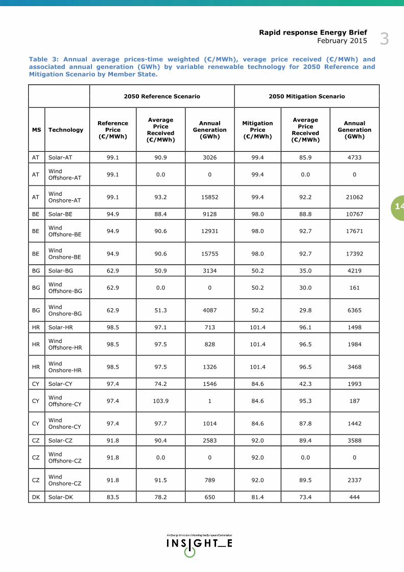
Table 3: Annual average prices-time weighted (€/MWh), verage price received (€/MWh) and

associated annual generation (GWh) by variable renewable technology for 2050 Reference and Mitigation Scenario by Member State.

2050 Reference Scenario 2050 Mitigation Scenario

MS Technology Reference

Price (€/MWh)

Average Price

Received (€/MWh)

Annual Generation

(GWh)

Mitigation Price

(€/MWh)

Average Price

Received (€/MWh)

Annual Generation

(GWh)

AT Solar-AT 99.1 90.9 3026 99.4 85.9 4733

AT Wind Offshore-AT

99.1 0.0 0 99.4 0.0 0

AT Wind Onshore-AT

99.1 93.2 15852 99.4 92.2 21062

BE Solar-BE 94.9 88.4 9128 98.0 88.8 10767

BE Wind Offshore-BE

94.9 90.6 12931 98.0 92.7 17671

BE Wind Onshore-BE

94.9 90.6 15755 98.0 92.7 17392

BG Solar-BG 62.9 50.9 3134 50.2 35.0 4219

BG Wind Offshore-BG

62.9 0.0 0 50.2 30.0 161

BG Wind Onshore-BG

62.9 51.3 4087 50.2 29.8 6365

HR Solar-HR 98.5 97.1 713 101.4 96.1 1498

HR Wind Offshore-HR

98.5 97.5 828 101.4 96.5 1984

HR Wind Onshore-HR

98.5 97.5 1326 101.4 96.5 3468

CY Solar-CY 97.4 74.2 1546 84.6 42.3 1993

CY Wind Offshore-CY

97.4 103.9 1 84.6 95.3 187

CY Wind Onshore-CY

97.4 97.7 1014 84.6 87.8 1442

CZ Solar-CZ 91.8 90.4 2583 92.0 89.4 3588

CZ Wind Offshore-CZ

91.8 0.0 0 92.0 0.0 0

CZ Wind Onshore-CZ

91.8 91.5 789 92.0 89.5 2337

DK Solar-DK 83.5 78.2 650 81.4 73.4 444

Rapid response Energy Brief

February 2015 3

15

DK Wind Offshore-DK

83.5 59.0 7862 81.4 51.0 8589

DK Wind Onshore-DK

83.5 58.8 18383 81.4 50.9 19932

EE Solar-EE 81.0 0.0 0 75.2 0.0 0

EE Wind

Offshore-EE 81.0 76.7 749 75.2 67.7 973

EE Wind Onshore-EE

81.0 76.7 4601 75.2 67.7 6175

FI Solar-FI 77.1 73.1 64 71.2 65.7 67

FI Wind Offshore-FI

77.1 66.8 3527 71.2 57.7 3527

FI Wind Onshore-FI

77.1 66.8 11098 71.2 57.7 14057

FR Solar-FR 89.5 79.5 25443 86.4 69.2 32772

FR Wind Offshore-FR

89.5 76.4 64063 86.4 75.8 65848

FR Wind Onshore-FR

89.5 76.4 102780 86.4 75.8 116095

DE Solar-DE 93.9 77.1 69966 96.0 77.7 73642

DE Wind Offshore-DE

93.9 89.9 51198 96.0 91.5 51276

DE Wind Onshore-DE

93.9 88.9 152688 96.0 90.5 195526

GR Solar-GR 90.7 66.1 10251 73.1 24.6 13516

GR Wind

Offshore-GR 90.7 87.2 397 73.1 63.3 5085

GR Wind Onshore-GR

90.7 83.7 19897 73.1 56.3 23389

HU Solar-HU 100.8 98.9 1378 102.2 98.3 1701

HU Wind Offshore-HU

100.8 0.0 0 102.2 0.0 0

HU Wind Onshore-HU

100.8 99.2 2671 102.2 99.8 3868

IE Solar-IE 79.7 74.8 974 64.7 83.2 598

IE Wind Offshore-IE

79.7 55.1 2105 64.7 51.9 2873

IE Wind Onshore-IE

79.7 52.5 17128 64.7 25.8 29350

IT Solar-IT 90.3 63.3 67590 88.0 45.1 95710

Rapid response Energy Brief

February 2015 3

16

IT Wind Offshore-IT

90.3 78.9 8078 88.0 88.6 12493

IT Wind Onshore-IT

90.3 77.4 53857 88.0 83.5 67121

LT Solar-LT 84.7 0.0 0 77.9 0.0 0

LT Wind

Offshore-LT 84.7 67.5 142 77.9 56.5 142

LT Wind Onshore-LT

84.7 67.5 1269 77.9 56.5 1561

LV Solar-LV 83.2 84.9 1 76.8 77.1 1

LV Wind Offshore-LV

83.2 66.3 988 76.8 55.5 1100

LV Wind Onshore-LV

83.2 66.3 1250 76.8 55.5 2233

LU Solar-LU 97.9 89.6 906 100.0 87.5 1677

LU Wind Offshore-LU

97.9 0.0 0 100.0 0.0 0

LU Wind Onshore-LU

97.9 90.6 772 100.0 91.5 1579

MT Wind Offshore-MT

88.5 88.0 298 83.1 85.6 311

MT Wind Onshore-MT

88.5 89.5 206 83.1 85.6 311

NL Wind Offshore-NL

96.1 88.7 24180 93.2 79.1 35120

NL Wind Onshore-NL

96.1 88.7 31521 93.2 79.1 41797

PL Wind

Offshore-PL 87.8 81.7 3095 93.1 86.0 6107

PL Wind Onshore-PL

87.8 81.7 16433 93.1 86.0 18779

PT Wind Offshore-PT

75.2 63.3 705 70.7 79.0 697

PT Wind Onshore-PT

75.2 57.3 23544 70.7 71.2 24219

RO Wind Offshore-RO

66.1 55.5 869 52.4 36.0 2690

RO Wind Onshore-RO

66.1 55.5 8618 52.4 36.0 16278

Rapid response Energy Brief

February 2015 3

17

SK Wind Offshore-SK

94.3 0.0 0 94.8 0.0 0

SK Wind Onshore-SK

94.3 91.9 1440 94.8 92.3 2379

SI Wind Offshore-SI

100.0 0.0 0 101.4 0.0 0

SI Wind Onshore-SI

100.0 98.7 1434 101.4 99.8 1420

ES Solar-ES 90.9 76.2 39821 79.4 39.2 69993

ES Wind Offshore-ES

90.9 85.6 288 79.4 93.4 269

ES Wind Onshore-ES

90.9 83.0 120609 79.4 85.4 138497

SE Wind Offshore-SE

79.2 60.5 3365 75.4 54.0 2337

SE Wind Onshore-SE

79.2 60.5 22533 75.4 54.0 23708

UK Wind Offshore-UK

81.9 64.0 99214 75.7 51.1 136970

UK Wind Onshore-UK

81.9 63.9 103833 75.7 51.1 133886