Quantifying the Impact of Exogenous Non …epubs.surrey.ac.uk/380519/2/SEEDS123.pdfSEEDS SURREY...

SEEDS SURREY Surrey Energy Economics ENERGY Discussion paper Series ECONOMICS CENTRE

Quantifying the Impact of ExogenousNon-Economic Factors on UK Transport Oil Demand

David C Broadstock and Lester C Hunt

May 2009

SEEDS 123 Department of Economics ISSN 1749-8384 University of Surrey

The Surrey Energy Economics Centre (SEEC) consists of members of the Department of Economics who work on energy economics, environmental economics and regulation. The Department of Economics has a long-standing tradition of energy economics research from its early origins under the leadership of Professor Colin Robinson. This was consolidated in 1983 when the University established SEEC, with Colin as the Director; to study the economics of energy and energy markets.

SEEC undertakes original energy economics research and since being established it has conducted research across the whole spectrum of energy economics, including the international oil market, North Sea oil & gas, UK & international coal, gas privatisation & regulation, electricity privatisation & regulation, measurement of efficiency in energy industries, energy & development, energy demand modelling & forecasting, and energy & the environment. SEEC also encompasses the theoretical research on regulation previously housed in the department's Regulation & Competition Research Group (RCPG) that existed from 1998 to 2004.

SEEC research output includes SEEDS - Surrey Energy Economic Discussion paper Series (details at www.seec.surrey.ac.uk/Research/SEEDS.htm) as well as a range of other academic papers, books and monographs. SEEC also runs workshops and conferences that bring together academics and practitioners to explore and discuss the important energy issues of the day.

SEEC also attracts a large proportion of the department’s PhD students and oversees the MSc in Energy Economics & Policy. Many students have successfully completed their MSc and/or PhD in energy economics and gone on to very interesting and rewarding careers, both in academia and the energy industry.

Enquiries: Director of SEEC and Editor of SEEDS: Lester C Hunt SEEC, Department of Economics, University of Surrey, Guildford GU2 7XH, UK. Tel: +44 (0)1483 686956 Fax: +44 (0)1483 689548 Email: [email protected] www.seec.surrey.ac.uk

i

___________________________________________________________

Surrey Energy Economics Centre (SEEC)

Department of Economics University of Surrey

SEEDS 123 ISSN 1749-8384

___________________________________________________________

QUANTIFYING THE IMPACT OF EXOGENOUS NON-ECONOMIC FACTORS ON UK TRANSPORT OIL DEMAND

David C Broadstock and Lester C Hunt

May 2009

___________________________________________________________

This paper may not be quoted or reproduced without permission.

ii

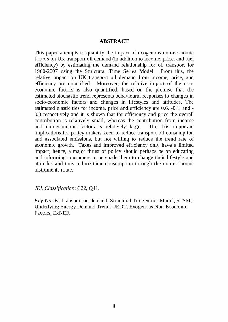
ABSTRACT

This paper attempts to quantify the impact of exogenous non-economic factors on UK transport oil demand (in addition to income, price, and fuel efficiency) by estimating the demand relationship for oil transport for 1960-2007 using the Structural Time Series Model. From this, the relative impact on UK transport oil demand from income, price, and efficiency are quantified. Moreover, the relative impact of the non-economic factors is also quantified, based on the premise that the estimated stochastic trend represents behavioural responses to changes in socio-economic factors and changes in lifestyles and attitudes. The estimated elasticities for income, price and efficiency are 0.6, -0.1, and -0.3 respectively and it is shown that for efficiency and price the overall contribution is relatively small, whereas the contribution from income and non-economic factors is relatively large. This has important implications for policy makers keen to reduce transport oil consumption and associated emissions, but not willing to reduce the trend rate of economic growth. Taxes and improved efficiency only have a limited impact; hence, a major thrust of policy should perhaps be on educating and informing consumers to persuade them to change their lifestyle and attitudes and thus reduce their consumption through the non-economic instruments route. JEL Classification: C22, Q41. Key Words: Transport oil demand; Structural Time Series Model, STSM; Underlying Energy Demand Trend, UEDT; Exogenous Non-Economic Factors, ExNEF.

Quantifying the Impact of Exogenous Non‐Economic Factors on UK Transport Oil Demand Page 1 of 15

Quantifying the Impact of Exogenous Non-Economic Factors on UK Transport Oil Demand

David C Broadstocka and Lester C Huntb

a Surrey Energy Economics Centre (SEEC) & Research Group on Lifestyles Values and Environment (RESOLVE), Department of Economics. University of Surrey, Guildford,

Surrey, GU2 7XH, UK.

b Corresponding Author: Surrey Energy Economics Centre (SEEC) & Research Group on Lifestyles Values and Environment (RESOLVE), Department of Economics. University of Surrey, Guildford,

Surrey, GU2 7XH, UK. Tel: +44(0)1483 686956, Fax: +44(0)1483 689548, Email: [email protected]

1. Introduction

As a level one student of economics is taught very early on, demand for a good or

service is a function of income, price, and ‘tastes’. Tastes describe the utility a

consumer gets from the goods consumed and, according to Begg’s (2009) level one

text, “depend on culture, history, familiarity, relationships with others, advertising,

and so on” (p. 34). Moreover, explaining the influence of ‘tastes’ is not the role of

economists it is the “role of other social sciences, like psychology and sociology”

(Begg, 2009, p. 34). So for economists these ‘tastes’ are often regarded as

‘exogenous’ to the model; part of the ‘ceteris paribus’ assumption behind a particular

demand curve and although there is usually some discussion and analysis of how

demand might be affected by a change in ‘tastes’, there is no real discussion of the

importance of these ‘tastes’ relative to the economic factors.

However, given the ‘urgency’ of the energy and environmental policy agenda and the

arguments put forward in some quarters for non-economic solutions it appears

imperative that an attempt is made to quantify the impact of these exogenous ‘taste’

factors. Given also that carbon predominately arises from the consumption of energy


then there is arguably a need to understand what contribution behaviourally focussed

interventions, such as educational schemes and other government initiatives, might

have on transport oil demand. In other words what contribution do exogenous non-

economic factors (of ExNEF for short) play in driving transport oil demand? 1

This paper therefore considers the modelling of UK transport oil demand and attempts

to isolate the traditional ‘economic drivers’ of income and price from the ‘exogenous

non-economic factors’. A summary of elasticities from previous fuel demand studies,

taken from Goodwin et al. (2004), is given in Table 1. This will serve as a benchmark

for the empirical results presented in this paper, however, the results summarised in

Table 1 are based upon studies in which the consumer ‘tastes’ or ExNEF were not

controlled – effectively ignored. This is arguably a shortcoming given the current

energy and environmental policy agenda with policy makers desperate to devise a

range of workable and achievable policies to help curtail future energy demand and

hence CO2 emissions. However, a useful review of the manner in which surface

transport carbon emissions reductions might be achieved through behavioural and

technological change is given in UKERC (2009), further reinforcing that the ExNEF

should at least feature in a general transport (energy) demand modelling framework.

Table 1: Summary of elasticities from previous studies Reference Elasticity w.r.t. price Elasticity w.r.t. income

Short-run Long-run Short-run Long-run Goodwin (1992) -0.27 -0.73 n/a n/a Espey (1998) -0.26 -0,58 0.47 0.88 Graham and Glaister (2002) -0.2 to -0.3 -0.6 to -0.8 0.35 to 0.55 1.1 to 1.3

Notes • taken from Goodwin et al. (2004)

1 This work is part of on-going research in RESOLVE attempting to quantify the impact of ExNEF on consumer demand and expenditure; see, for example, Chitnis and Hunt (2009a and 2009b).


The order of this paper is as follows. Following from this introduction the next

section outlines the estimation methodology, including a brief discussion of the data.

Section 3 presents the results and Section 4 summarises and concludes with a brief

discussion.

2. Methodology

The model is based on the structural time series model (STSM) developed by Harvey

(1989 & 1997) and advocated for the use when modelling energy demand functions

by Hunt et al. (2003a & 2003b) and Hunt and Ninomiya (2003) who argue that a

stochastic trend, coined the underlying energy demand trend (or UEDT for short)

should be estimated. They argue that the UEDT is driven by exogenous technical

progress of the capital and appliance stock, such as vehicle efficiency, etc and other

socio economic factors termed ‘consumer tastes’ such as driving children to school

etc. (see Hunt and Ninomiya, 2003). However, here, an attempt is made to separate

out the effect of technical progress and fuel efficiency from the UEDT by

incorporating an appropriate efficiency variable. Consequently, the estimated UEDT

here only picks up the effects of the ‘tastes’ referred to by the simple economic model

above, i.e. it captures the effects of values, lifestyles, etc.

The following STSM is therefore specified for UK transport oil demand:

ot

ott

oft

opt

oyt fpoyeo εμααα ++++= (1)

ot

ot

ot

ot ηβμμ ++= −− 11 (2)

ot

ot

ot ξββ += −1 (3)


where ( )2,0~ oeot NID σε , ( )2,0~ oNIDo

t ηση and ( )2,0~ oNIDo

t ξσξ . eot is the natural

logarithm of transport oil consumption, yt is the natural logarithm of income, pot is the

natural logarithm of the real transport oil price, ft is the natural logarithm of car fuel

efficiency and otε the error term. o

yα , opα and o

fα represent the (long-run) oil

transport demand income, price, and fuel efficiency elasticities respectively.2

Equations (2) and (3) represent the UEDT (without fuel efficiency) for transport oil

demand, otμ , made up of the two components, the level and slope respectively. This is

a stochastic trend dependent upon the variances 2oη

σ and 2oζ

σ (also known as the

hyperparameters), the larger the hyperparameters the greater the stochastic

movements in the trend. In the limiting case when the hyperparameters are equal to

zero, the model collapses to a conventional deterministic time trend regression. This

therefore gives a number of alternative forms of the stochastic trend depending on the

values of the hyperparameters.3

The initial model to be estimated therefore consists of an Autoregressive Distributed

Lag version of Equation (1) with lags of 4 years plus Equations (2) and (3), over the

period 1964-2003, keeping 2004-2007 for predictive failure tests. All disturbance

terms are assumed independent and uncorrelated with each other. The estimation is

carried out by maximum likelihood and the hyperparameters are obtained from a

smoothing algorithm using the Kalman filter. The preferred parsimonious

2 When actually estimating the model, a general autoregressive distributed lag model is estimated and the preferred parsimonious model found by testing down using the ‘general to specific’ methodology. However, for the preferred models presented below the parsimonious model is always that given by Equation (1).

3 A classification of the different types is given in Table 9.2 in Hunt et al. (2003b).


specification of the model is selected by testing down from the general equation by

eliminating statistically insignificant variables, whilst ensuring that the equation

residuals (similar to those from ordinary regression) pass a range of diagnostic tests, a

set of auxiliary residuals (irregular, level and slope) do not suffer from non-normality,

and the model passes predictive failure tests over the 2004-2007 period. The

preferred specification is then re-estimated over the longest data period available, up

to 2007 and as far back to 1960 as possible, depending on whether any lag variables

remain in the model. The software package STAMP 6.3 (Koopman et al., 2000) is

used for all estimation.

Using the results over the longer period for the preferred specification, the

contributions of income, price, fuel efficiency and ExNEF to the annual change in oil

demand are constructed from the following:

∧∧∧∧∧

Δ+Δ+Δ+Δ=Δ ott

oft

opt

oyt fpoyeo μααα (4)

where , ,∧∧

op

oy αα and

∧ofα are the estimated income, price and fuel elasticities respectively

and∧

otμ the estimated UEDT. Therefore, , , , t

oft

opt

oy fpoy ΔΔΔ

∧∧∧

ααα and∧

Δ otμ represent the

estimated contributions to the change in UK transport oil demand (in logs), from

income, the real price of oil, car fuel efficiency, and ExNEF respectively.4

4 Note, that given that the estimated preferred models presented below do not have any lags the contributions are easily calculated in this way. Furthermore, given the model is in logs the change approximates the percentage change.


3. Data and Results

Data

The UK annual data set covers the period 1960-2007 with the energy consumption

and price data taken from the Digest of UK Energy Statistics (DUKES) and the

income data from the UK Office of National statistics (www.statistics.gov.uk). These

are supported with data on total vehicle kilometres travelled in the UK taken from the

UK Department for Transport (http://www.dft.gov.uk/pgr/statistics/) used to derive

the efficiency term. The variables used in estimation are as follows:

EO = total transport oil consumption in thousand tonnes of oil;

Y = GDP at £million 2003 market prices

PO = real price of transport oil consumption in 2003£/litre5

F = car fuel efficiency in miles per gallon (mpg). 6

5 The price series for gasoline demand is made up of a number of separate grades of gasoline. Therefore, a quantity-weighted average of the series is defined including the following components: 2 Star (1960-1989), 3 Star (1967-1989), 4 Star (1960-2005), 5 Star (1961-1979), Super Premium Unleaded (1990-2005) and Premium Unleaded (1988-2005). Noting that a number of the fuel types of the period either/both entered or left the market for various reasons. Unique price series are not available for 3 Star and 5 Star fuel, therefore it is assumed that they have the same prices as 4 Star fuel, which is much closer in quality than 2 Star fuel. Using superscripts to denote the different components of gasoline, the calculation of the nominal weighted average series can be expressed as;

][)]*()*()*()*()*()*[(

5432

54443422

SPUt

PUt

start

start

start

start

SPUt

SPUt

PUt

SPt

start

start

start

start

start

start

start

start

qqqqqqqpqpqpqpqpqp

++++++++++

This was then deflated by the GDP deflator at 2003 prices to give the real price of gasoline (PO) at 2003£/litre.

6 The fuel efficiency is expressed as mpg; however, it should be noted that some authors measure this in litres per 100km; although many previous studies do use as mpg as the efficiency metric, as shown in Table 2 in Bonilla and Foxon (2009, p. 67),


Figure 1: UK Transport oil consumption a) EOt (million tonnes) b) Δeot (annual change in logs)

0

5000

10000

15000

20000

25000

30000

35000

40000

45000

1960

1961

1962

1963

1964

1965

1966

1967

1968

1969

1970

1971

1972

1973

1974

1975

1976

1977

1978

1979

1980

1981

1982

1983

1984

1985

1986

1987

1988

1989

1990

1991

1992

1993

1994

1995

1996

1997

1998

1999

2000

2001

2002

2003

2004

2005

2006

2007

‐0.04

‐0.02

0

0.02

0.04

0.06

0.08

0.1

0.12

1960

1961

1962

1963

1964

1965

1966

1967

1968

1969

1970

1971

1972

1973

1974

1975

1976

1977

1978

1979

1980

1981

1982

1983

1984

1985

1986

1987

1988

1989

1990

1991

1992

1993

1994

1995

1996

1997

1998

1999

2000

2001

2002

2003

2004

2005

2006

2007

Figure 2: GDP a) Yt (£million 2003 Market Prices) b) Δyt (annual change in logs)

0

200000

400000

600000

800000

1000000

1200000

1400000

1960

1961

1962

1963

1964

1965

1966

1967

1968

1969

1970

1971

1972

1973

1974

1975

1976

1977

1978

1979

1980

1981

1982

1983

1984

1985

1986

1987

1988

1989

1990

1991

1992

1993

1994

1995

1996

1997

1998

1999

2000

2001

2002

2003

2004

2005

2006

2007

‐0.03

‐0.02

‐0.01

0

0.01

0.02

0.03

0.04

0.05

0.06

0.07

0.08

1960

1961

1962

1963

1964

1965

1966

1967

1968

1969

1970

1971

1972

1973

1974

1975

1976

1977

1978

1979

1980

1981

1982

1983

1984

1985

1986

1987

1988

1989

1990

1991

1992

1993

1994

1995

1996

1997

1998

1999

2000

2001

2002

2003

2004

2005

2006

2007

Figure 3: Real price of UK transport oil a) POt (2003pence/gallon) b) Δpot (annual change in logs)

50

55

60

65

70

75

80

85

90

1960

1961

1962

1963

1964

1965

1966

1967

1968

1969

1970

1971

1972

1973

1974

1975

1976

1977

1978

1979

1980

1981

1982

1983

1984

1985

1986

1987

1988

1989

1990

1991

1992

1993

1994

1995

1996

1997

1998

1999

2000

2001

2002

2003

2004

2005

2006

2007 ‐0.2

‐0.15

‐0.1

‐0.05

0

0.05

0.1

0.15

0.2

0.25

0.3

1960

1961

1962

1963

1964

1965

1966

1967

1968

1969

1970

1971

1972

1973

1974

1975

1976

1977

1978

1979

1980

1981

1982

1983

1984

1985

1986

1987

1988

1989

1990

1991

1992

1993

1994

1995

1996

1997

1998

1999

2000

2001

2002

2003

2004

2005

2006

2007

Figure 4: Average vehicle fuel efficiency in mpg(Ft) a) Ft (mpg) b) Δft (annual change in logs)

21

22

23

24

25

26

27

28

29

1960

1961

1962

1963

1964

1965

1966

1967

1968

1969

1970

1971

1972

1973

1974

1975

1976

1977

1978

1979

1980

1981

1982

1983

1984

1985

1986

1987

1988

1989

1990

1991

1992

1993

1994

1995

1996

1997

1998

1999

2000

2001

2002

2003

2004

2005

2006

2007

‐0.03

‐0.02

‐0.01

0

0.01

0.02

0.03

0.04

0.05

0.06

1960

1961

1962

1963

1964

1965

1966

1967

1968

1969

1970

1971

1972

1973

1974

1975

1976

1977

1978

1979

1980

1981

1982

1983

1984

1985

1986

1987

1988

1989

1990

1991

1992

1993

1994

1995

1996

1997

1998

1999

2000

2001

2002

2003

2004

2005

2006

2007


The data for oil consumption and the economic drivers (income and price) are shown

in Figures 1 to 3. Figure 1a illustrates the general strong growth in UK transport oil

consumption through the 1960s, 1970s and 1980s, but a general slowing in growth

since the early 1990s. This is also shown in Figure 1b, which illustrates the annual

changes in UK transport oil demand (in natural logarithms) that the ‘contributions

methodology’ attempts to explain. Figures 2a and 2b illustrate the general upward

trend in UK GDP other than during the recessions in the 1970s, 1980s and 1990s, and

Figures 2a and 2b illustrate the volatility in real transport oil prices including the large

increases in the early and late 1970s, the fall in the mid 1980s and the general increase

since then. Figures 4a and 4b illustrate that car fuel efficiency has generally increased

since the early 1980s.

Results.

The results for the estimation of the model above are given in Table 2 with the

estimated trends given in Figure 5. Specification I is the preferred model over the

period 1964-2003 after the testing procedure outlined above, which has no dynamics

despite starting with lags of 4 years on all the data. Nevertheless, it still fits the data

well; passing all diagnostic tests for serial correlation, heteroscedasticity, non-

normality7 and predictive failure. Furthermore, the restriction of a deterministic trend

is rejected via the Likelihood Ratio (LR) test.

7 Note, that following Harvey and Koopman (1992), impulse dummies are included for 1979 and 1980 given some evidence of non-normality of the auxiliary residuals.


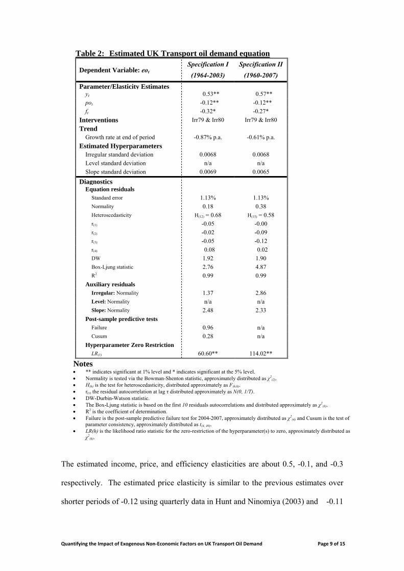
Table 2: Estimated UK Transport oil demand equation

Dependent Variable: eot Specification I Specification II

(1964-2003) (1960-2007)

Parameter/Elasticity Estimates yt 0.53** 0.57** pot -0.12** -0.12** ft -0.32* -0.27*

Interventions Irr79 & Irr80 Irr79 & Irr80 Trend

Growth rate at end of period -0.87% p.a. -0.61% p.a. Estimated Hyperparameters

Irregular standard deviation 0.0068 0.0068 Level standard deviation n/a n/a Slope standard deviation 0.0069 0.0065

Diagnostics Equation residuals

Standard error 1.13% 1.13% Normality 0.18 0.38 Heteroscedasticity H(12) = 0.68 H(15) = 0.58 r(1) -0.05 -0.00 r(2) -0.02 -0.09 r(3) -0.05 -0.12 r(4) 0.08 0.02 DW 1.92 1.90 Box-Ljung statistic 2.76 4.87 R2 0.99 0.99

Auxiliary residuals Irregular: Normality 1.37 2.86 Level: Normality n/a n/a Slope: Normality 2.48 2.33

Post-sample predictive tests Failure 0.96 n/a Cusum 0.28 n/a

Hyperparameter Zero Restriction LR(1) 60.60** 114.02**

Notes • ** indicates significant at 1% level and * indicates significant at the 5% level. • Normality is tested via the Bowman-Shenton statistic, approximately distributed as χ2

(2). • H(h) is the test for heteroscedasticity, distributed approximately as F(h,h). • r(τ) the residual autocorrelation at lag τ distributed approximately as N(0, 1/T). • DW-Durbin-Watson statistic. • The Box-Ljung statistic is based on the first 10 residuals autocorrelations and distributed approximately as χ2

(8). • R2 is the coefficient of determination. • Failure is the post-sample predictive failure test for 2004-2007, approximately distributed as χ2

(4) and Cusum is the test of parameter consistency, approximately distributed as t(4, 40).

• LR(h) is the likelihood ratio statistic for the zero-restriction of the hyperparameter(s) to zero, approximately distributed as χ2

(h).

The estimated income, price, and efficiency elasticities are about 0.5, -0.1, and -0.3

respectively. The estimated price elasticity is similar to the previous estimates over

shorter periods of -0.12 using quarterly data in Hunt and Ninomiya (2003) and -0.11


using annual data in Dimitropoulos et al. (2003). However, the estimated income

elasticity is a little lower compared to the 0.80 in Hunt and Ninomiya (2003) and the

0.81 in Dimitropoulos et al. (2003). These, however, did not include an efficiency

term (instead it was assumed that this was captured in the UEDT); but despite this, the

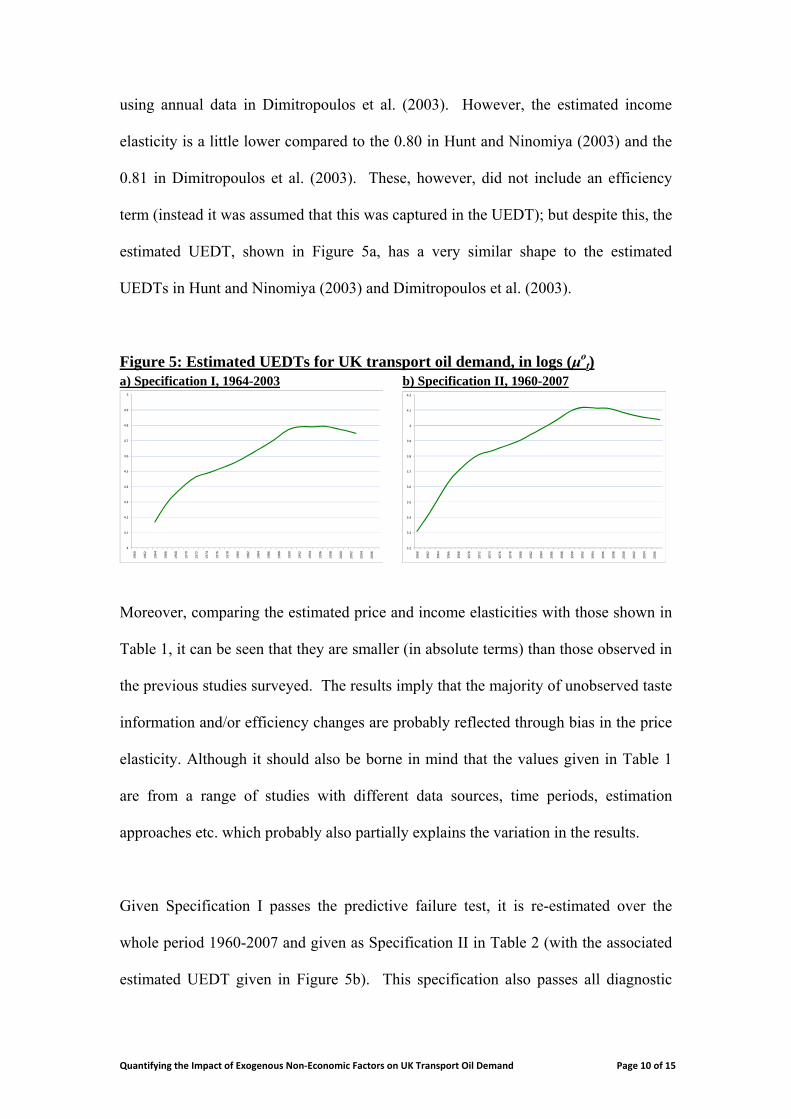
estimated UEDT, shown in Figure 5a, has a very similar shape to the estimated

UEDTs in Hunt and Ninomiya (2003) and Dimitropoulos et al. (2003).

Figure 5: Estimated UEDTs for UK transport oil demand, in logs (μot)

a) Specification I, 1964-2003 b) Specification II, 1960-2007

4

4.1

4.2

4.3

4.4

4.5

4.6

4.7

4.8

4.9

5

1960

1962

1964

1966

1968

1970

1972

1974

1976

1978

1980

1982

1984

1986

1988

1990

1992

1994

1996

1998

2000

2002

2004

2006

3.2

3.3

3.4

3.5

3.6

3.7

3.8

3.9

4

4.1

4.2

1960

1962

1964

1966

1968

1970

1972

1974

1976

1978

1980

1982

1984

1986

1988

1990

1992

1994

1996

1998

2000

2002

2004

2006

Moreover, comparing the estimated price and income elasticities with those shown in

Table 1, it can be seen that they are smaller (in absolute terms) than those observed in

the previous studies surveyed. The results imply that the majority of unobserved taste

information and/or efficiency changes are probably reflected through bias in the price

elasticity. Although it should also be borne in mind that the values given in Table 1

are from a range of studies with different data sources, time periods, estimation

approaches etc. which probably also partially explains the variation in the results.

Given Specification I passes the predictive failure test, it is re-estimated over the

whole period 1960-2007 and given as Specification II in Table 2 (with the associated

estimated UEDT given in Figure 5b). This specification also passes all diagnostic


tests and the estimated parameters are very similar: about 0.6, -0.1, and -0.3 for the

income, price and efficiency elasticities respectively. Moreover, the estimated UEDT

has a similar shape to that for Specification I. Therefore, Specification II is used for

the remainder of the analysis and discussion; it is used to estimate the contributions of

the different drivers of the change in UK transportation oil demand, as specified in

Equation (4) above. This is illustrated in Figure 6 and summarised in Table 3.8

Figure 6: Contributions to change in UK transport oil demand, in logs (Δeot)

‐0.0800

‐0.0600

‐0.0400

‐0.0200

0.0000

0.0200

0.0400

0.0600

0.0800

0.1000

1960

1961

1962

1963

1964

1965

1966

1967

1968

1969

1970

1971

1972

1973

1974

1975

1976

1977

1978

1979

1980

1981

1982

1983

1984

1985

1986

1987

1988

1989

1990

1991

1992

1993

1994

1995

1996

1997

1998

1999

2000

2001

2002

2003

2004

2005

2006

2007

po contribution y contribution f contributionEx‐NEF contribution Δeo

It is clear from Figure 6 that the contribution of GDP in driving the change in

transport oil demand is important and relatively stable other than in times of

recessions; remaining a relatively important positive driver in all periods identified in

Table 3. In contrast, the contribution of prices is relatively small other than during the

8 Admittedly, the chosen dates for the different periods in Table 3 is arbitrary, but roughly coincides with the oil price hikes (and subsequent recessions) in the 1970s, the oil price collapse of the mid 1980s, and the recession of the early 1990s.


very high price changes, in particular the period 1985-1991. Similarly, the

contribution from fuel efficiency changes is relatively small over all periods, whereas,

ExNEF appears to have had an important positive impact until the early 1990s. From

1960 to 1973 ExNEF appears to have dominated the contribution to the change in

transport oil demand - being the main reason for the strong growth during this period.

Interestingly the strong positive contribution of ExNEF up to the 1990s is generally

reversed from the early 1990s. ExNEF makes a negative average contribution since

1991, so that despite the relative strong positive contribution from income, the actual

growth in oil transport demand slowed down considerably during the period 1991-

2007, driven primarily by the negative contribution from ExNEF (and the smaller

contributions from price and efficiency). Thus there appears to be a marked

‘behaviour change’ over this latest period, perhaps reflecting greater consumer

environmental awareness and a resultant change in ‘lifestyle’ and attitudes’.

Table 3: Summary of the contribution to the average percentage per annum change in UK transport oil demand, in logs (Δeot)

Period Contribution from: Total change

in eo y po f ExNEF

1960-1973 1.76 0.20 0.12 3.96 6.23 1973-1985 0.81 -0.28 -0.18 1.43 1.79 1985-1991 1.41 0.59 -0.24 1.96 3.79 1991-2007 1.56 -0.23 -0.19 -0.45 0.69 1960-2007 1.41 -0.02 -0.11 1.56 2.87

Notes • Following from Equation (4) the annual changes per annum contributions are approximated as

follows: %

nyt

oy Δ∧

α , %

npot

op Δ∧

α , %

nft

of Δ

∧

α ,and %n

ot

∧

Δ μ for the contributions of GPD (y), price (po), fuel

efficiency (f), and exogenous non-economic factors (ExNEF) respectively. (The total change

being approximated by % neotΔ .) Where n is the span of years that the change is calculated.


5. Concluding remarks

This paper is, as far as is known, the first attempt to use time series econometrics to

quantify both the economic and the non-economic drivers of UK transport oil demand.

This quantification shows that income generally makes an important positive

contribution to driving the change in UK road transport oil demand given the

estimated income elasticity of about 0.6 and the size of the changes in income.

Whereas the estimated price and fuel efficiency elasticities of about -0.1 and -0.3 are

smaller (in absolute terms); hence the estimated contributions from price and fuel

efficiency are relatively small. Moreover, the quantification using the estimated non-

linear UEDT shows that the non-economic behavioural factor ExNEF makes a non-

trivial and positive contribution up until the early 1990s. However, since then, there

appears to be an important behaviour change with the non-economic factors making a

small but still important negative contribution to the change in the UK road transport

oil demand. Moreover, the estimated ExNEF in the later periods suggests that

consumer tastes are no longer driving demand up, or put another way; rises in

transport oil demand are being driven predominantly by income more than ever before;

particularly given fuel efficiency continues to improve.

This finding has important implications for policy makers wishing to curtail the

growth in transport oil demand in the UK. The analysis suggests that the effect of

taxes and increased fuel efficiency would be very limited given the estimated

elasticities and subsequent contributions; although in a rounded policy package, there

is no reason why these should not be used – provided their limitations are recognised.

This therefore leaves policy makers with the main choice between attempting to

reduce the trend rate of growth of the economy and/or acting on the non-economic


aspects of behaviour change. However, in a political world where, over the longer

term, reduced economic growth is unlikely to be an option for elected policy makers,

it leaves action on behaviour as crucial. In other words, assuming policy makers wish

to reduce the growth in transport oil demand and hence emissions, but do not (or

cannot) curtail economic growth and the effect of taxes and increased fuel efficiency

are limited, then the policy action needs to be on changing non-economic behaviour –

or those ‘simple’ tastes alluded to in level one economics texts. A main thrust of

policy would therefore need to concentrate on educating and informing consumers in

an attempt to encourage them to reduce their consumption of transport oil and hence

emissions through the non-economic instruments route.

Acknowledgements This work is part of the interdisciplinary research programme undertaken by the Research Group on Lifestyles, Values, and the Environment (RESOLVE) funded by the Economic and Social Research Council (ESRC) and their support is gratefully acknowledged. The authors are grateful for comments on earlier drafts of the work presented at the 1st Empirical Methods in Energy Economics Workshop (EMEE), Zurich, Switzerland, 29th-30th August 2008 and an EPRG Energy and Environment Seminar, University of Cambridge, UK, 2nd March 2009. We would also like to thank the discussant of our paper at the EMEE conference, Adrian Müller, and Guy Judge for their comments and suggestions. Finally our thanks also to members of RESOLVE for many discussions about the work; in particular Mona Chitnis, Angela Druckman, and Tim Jackson. Of course, any errors and omissions are due to the authors.


References Begg, D., 2009. Foundations of Economics. (4th Edition), UK: McGraw-Hill Education.

Bonilla, D. and Foxon, T., 2009. Demand for new car fuel economy in the UK, 1970-2005. Journal of Transport Economics and Policy, 43, 55-83.

Chitnis, M. and Hunt, L. C., 2009a. What drives the change in UK household energy expenditure and associated CO2 emissions, economic or non-economic factors?, RESOLVE Working Paper, University of Surrey, forthcoming.

Chitnis, M. and Hunt, L. C., 2009b. Modelling UK household expenditure: economic versus non-economic drivers, RESOLVE Working Paper, University of Surrey, forthcoming.

Espey, M., 1998. Gasoline demand revisited: an international meta-analysis of elasticities. Energy Economics, 20, 273–295.

Goodwin, P., 1992. A review of new demand elasticities with special reference to short and long run effects of price changes. Journal of Transport Economics and Policy, 26, 155–163.

Goodwin, P., Dargay, J. and Hanly, M., 2004. Elasticities of road traffic and fuel consumption with respect to price and income. Transport Reviews, 24, 275-292.

Graham, D. and Glaister, S., 2002. The demand for automobile fuel: a survey of elasticities. Journal of Transport Economics and Policy, 36, 1–26.

Harvey, A. C., 1989. Forecasting, structural time series models and Kalman filter. Cambridge UK: Cambridge University Press.

Harvey, A. C., 1997. Trends cycles and autoregression. Economic Journal, 107, 192-201.

Harvey, A .C., and Koopman, S. J., 1992. Diagnostic checking of unobserved-components time series models. Journal of Business and Economics Statistics, 10, 377-389.

Hunt, L. C., Judge, G. and Ninomiya, Y., 2003a. Underlying trends and seasonality in UK energy demand: A sectoral analysis. Energy Economics, 25, 93-118.

Hunt, L. C., Judge, G. and Ninomiya, Y., 2003b. Modelling underlying energy demand trends. Chapter 9 in L. C. Hunt (Ed) Energy in a Competitive Market: Essays in Honour of Colin Robinson, Edward Elgar, UK. 140-174.

Hunt, L. C. and Ninomiya, Y., 2003. Unravelling trends and seasonality: A structural time series analysis of transport oil demand in the UK and Japan. The Energy Journal, 24, 63-96.

Koopman S. J., Harvey, A. C., Doornik, J. A. and Shephard, N., 2000. Stamp: structural time series analyser, modeller and predictor. London: Timberlake Consultants Press.

UKERC, 2009. What policies are effective at reducing carbon emissions from surface passenger transport? UK Energy Research Centre Report, 21st April, www.ukerc.ac.uk/MediaCentre/UKERCPressReleases/Releases2009/0904Transport.aspx.

Note: This paper may not be quoted or reproduced

without permission

Surrey Energy Economics Centre (SEEC) Department of Economics

University of Surrey Guildford

Surrey GU2 7XH

SURREY

ENERGY

ECONOMICS

DISCUSSION PAPER

SERIES

For further information about SEEC please go to:

www.seec.surrey.ac.uk

Quantifying the Impact of Exogenous Non …epubs.surrey.ac.uk/380519/2/SEEDS123.pdfSEEDS SURREY...

Documents

Transcript of Quantifying the Impact of Exogenous Non …epubs.surrey.ac.uk/380519/2/SEEDS123.pdfSEEDS SURREY...