QUANTIFYING DYNAMIC STABILITY OF MUSCULOSKELETAL SYSTEMS USING LYAPUNOV

EXPONENTS

SCOTT ENGLAND

Thesis presented to

The faculty of the Virginia Polytechnic Institute and State University

in partial fulfillment of the requirements for the degree of

Master of Science

in

Engineering Mechanics

Kevin P. Granata, Ph.D., Chair

Michael Madigan, Ph.D.

Dennis Hong, Ph.D.

September 13, 2005

Blacksburg, Virginia

Keywords: Stability, Lyapunov Exponents

QUANTIFYING DYNAMIC STABILITY OF MUSCULOSKELETAL SYSTEMS USING LYAPUNOV

EXPONENTS

Scott England

(ABSTRACT)

Increased attention has been paid in recent years to the means in which the body

maintains stability and the subtleties of the neurocontroller. Variability of kinematic data has

been used as a measure of stability but these analyses are not appropriate for quantifying stability

of dynamic systems. Response of biological control systems depend on both temporal and

spatial inputs, so means of quantifying stability should account for both. These studies utilized

tools developed for the analysis of deterministic chaos to quantify local dynamic stability of

musculoskeletal systems.

The initial study aimed to answer the oft assumed conjecture that reduced gait speeds in

people with neuromuscular impairments lead to improved stability. Healthy subjects walked on

a motorized treadmill at an array of speeds ranging from slow to fast while kinematic joint angle

data were recorded. Significant (p < 0.001) trends showed that stability monotonically decreased

with increasing walking speeds.

A second study was performed to investigate dynamic stability of the trunk. Healthy

subjects went through a variety of motions exhibiting either symmetric flexion in the sagittal

plane or asymmetric flexion including twisting at both low and high cycle frequencies. Faster

cycle frequencies led to significantly (p<0.001) greater instability than slower frequencies.

Motions that were hybrids of flexion and rotation were significantly (p<0.001) more stable than

motions of pure rotation or flexion.

Finding means of increasing dynamic stability may provide great understanding of the

neurocontroller as well as decrease instances of injury related to repetitive tasks. Future studies

should look in greater detail at the relationships between dynamic instability and injury and

between local dynamic stability and global dynamic stability.

ACKNOWLEDGEMENTS

The research described here was made possible through contributions from coworkers, family members and friends.

Dr Granata:

Thank you for being a great advisor, for believing in me and guiding this research.

Friends and Coworkers in the Musculoskeletal Biomechanics Laboratory:

Thank you for assistance in general especially Bradley Davidson and Greg Slota for their

help with teaching me the finer points of data collection and subtleties of Matlab.

Family:

Thanks you all for your love and support and instilling in me a love of science and

learning.

The mentors of FIRST Robotics team # 122:

Thank you for teaching me, inspiring me, and guiding my life in more ways than you can

imagine, especially Mr. Bill Reed, Mr. Ansel Butterfield, and Mr. Jeff Seaton.

iii

TABLE OF CONTENTS ABSTRACT ii ACKNOWLEDGEMENTS iii TABLE OF CONTENTS iv LIST OF FIGURES vi LIST OF TABLES viii CHAPTER 1 – INTRODUCTION 1 SPECIFIC AIMS 2 HYPOTHESES 2 CHAPTER 2 – BACKGROUND 3 2.1 Stability 3 2.1.1 Kinematic Variability 5

2.1.2 Inter-cycle Correlations 5 2.2 Lyapunov Analysis 9

2.2.1 Lyapunov Stability 9 2.2.2 Reconstructed Dynamics 10 2.2.3 Estimation of Maximum Lyapunov Exponent 15

2.3 Empirical Measurement of System Dynamics 17

2.3.1 Gait Study Data Collection 17 2.3.2 Back Study Data Collection 19

2.4 References 20 CHAPTER 3 – THE INFLUENCE OF GAIT SPEED ON LOCAL DYNAMIC STABILITY 24

3.1 Introduction 26 3.2 Methods 29 3.3 Results 35 3.4 Discussion 37 3.5 Acknowledgements 40 3.6 References 41

CHAPTER 4 – DYNAMIC STABILITY OF REPEATED TRUNK MOVEMENTS 44 4.1 Introduction 48 4.2 Materials and Methods 50 4.3 Results 56

iv

4.4 Discussion 58 4.5 Acknowledgement 60 4.6 References 61 CONCLUSIONS 65 APPENDICES 67 A. IRB Approval 67 B. Subject Consent Form 68 C. Lyapunov Analysis Flowchart 70 D. λMax Data Spreadsheets 71 E. Gait Analysis Matlab Program 78 F. Back Analysis Matlab Program 92 VITA 116

v

List of Figures

Figure 2.1 – Examples of attracting and Lyapunov stable fixed points 4 Figure 2.2 – A Poincare map demonstrating a stable system 8 Figure 2.3 – A traditional Lorenz attractor (A) and a Lorenz attractor reconstructed using the method of delays (B) 11 Figure 2.4 – Time delays selected from autocorrelation, C, and the average mutual information function, I, for a Roux attractor. The attractor reconstructed with time delays from each approach are in the upper right corner. Picture from Fraser and Swinney 1986, pp. 1135 (Reproduced with author’s permission). 13 Figure 2.5 – Plot of x(t) = sin(2πt) + cos(πt) with embedding dimension n=3 (A) and n=2 (B). Note the False Nearest Neighbor illustrated by the intersection at [-0.25,0.25] when n=2. 14 Figure 2.6 – Divergence and λMax for a Lorenz attractor 16 Figure 2.7 – Free body diagram of the inverted pendulum model 18

Figure 3.1 – (A) Reconstructed state-space kinematics of knee angle with 3 embedded dimensions. (B) Divergence of nearest neighbors with temporal variability permitted 31

Figure 3.2 – Plot of x(t) = sin(2πt) + cos(πt) with embedding dimension n=3 (A) and n=2 (B). Note the False Nearest Neighbor illustrated by the intersection at [-0.25,0.25] when n=2. 32

Figure 3.3 – Average logarithmic divergence vs time. The slope of the logarithmic relation from 0 to 1 stride represents λMax. 33 Figure 3.4 – Average λMax increased with walking velocity. This trend was observed when data were re-sampled to 3000 samples per 30 strides (A) and similarly when temporal variability was removed by re-sampling the data to 100 samples per stride (B) 35 Figure 4.1 – Experimental setup and schematic of the targeted movement task 51 Figure 4.2 – Example of a reconstructed movement trajectory with n=3 state-space dimensions. Although the movement data were analyzed with n=5, three embedding dimension is the largest that can be illustrated. 53 Figure 4.3 – Typical plot of the state-space expansion with time, ( ) ( )td

tty iln1

∆= . The

dashed line represents the best-fit line between t=0:1 cycles (with a cycle length of approximately 1.5 seconds for this trial). The slope of the best-fit line was used to

vi

represent the state-space expansion, i.e. local dynamic stability of the task. 55

Figure 4.4 – λMax values were greater during fast paced movement trials than slow paced cyclic movement. Values were also greater during asymmetric movement tasks than during sagittal mid-plane movements. Larger values of λMax represent less stable movement dynamics. 56

vii

List of Tables

Table 3.1 – Regression analysis results comparing λMax with walking velocity. Two of the three measurements were linearly related to velocity when stride-duration variability was removed (100 samples per stride). Two of the three measurements were related in a quadratic manner to walking velocity when stride-duration variability was retained (3000 samples per 30 strides). 36 Table 4.1 – Subject demographics and anthropometry 50

viii

Chapter 1 – Introduction

Poor dynamic stability may contribute to musculoskeletal injuries including low back

pain and those resulting from falls. In spite of extensive biomechanical study falls continue to be

a major source of injury and mortality for the elderly as well as a significant source of health care

expenses (Hausdorff 2001). Falls may be related to dynamic instability during functional

walking tasks. People suffering from peripheral neuropathy, a condition where nerves in distal

regions atrophy, are up to 1500 % more likely to injure themselves while walking than healthy

controls (Cavanagh 1992). Research has suggested that people with pathologies such as

peripheral neuropathy that affect neurocontroller function may exhibit gait patterns that differ

from healthy controls. These altered gait patterns may be attempts to improve stability in the

presence of detriments to the neurocontroller caused by pathology. Control of stability may also

influence risk of low back pain. Occupations that require repetitive trunk flexion have been

reported to have high incidence rates of low back pain (NIOSH 1999; Marras 1993).

Simultaneously, it is widely believed that instability of the spine leads to low back pain (Panjabi

2003). However, there are no existing measures of stability during dynamic trunk motions.

Efforts to quantify stability during dynamic motions may then increase our knowledge of the

behavior of the neurocontroller and aid in injury prevention and treatment of related pathologies.

Musculoskeletal injury from falls and low back pain combine to cost the American economy

over 120 billion dollars per year due to expenses ranging from medical bills to lost productivity

(Englander 1996; Luo 2004). Clearly there is a need to implement methods to quantify

neuromuscular stability of dynamic movement.

Quantifying stability is an inherently difficult task as requirements for maintaining

stability are dependent on the analyzed system. A comprehensive definition for stability in a

musculoskeletal system would cite it as the ability to maintain a desired trajectory despite the

presence of small kinematic perturbations or control errors. The ability to maintain stability

during a dynamic task may be key to injury prevention. Perhaps the most commonly found trait

in pathological gait that may be an attempt to increase stability is lower average walking velocity

when compared to healthy controls.

Movement velocity may influence stability by several possible means. Higher movement

velocity leads to elevated system momentum, which requires greater neuromuscular effort for

1

control. Increased rate of movement also reduces available time for neuromuscular reaction,

increasing the likelihood of loss of stability. Asymmetry of trunk flexion/extension movements

may also influence stability as a result of modified muscle recruitment and co-contraction

beyond the typical agonistic-antagonistic models in symmetric flexion/extension. Therefore the

goal of this study was to quantify dynamic stability of these musculoskeletal systems using an

approach developed for the analysis of deterministic chaos, Lyapunov exponents.

SPECIFIC AIMS 1. Quantify effects of increased walking velocity on dynamic stability of lower extremity

during gait.

2. Quantify effects of cycle frequency and symmetry of motion on trunk stability.

HYPOTHESES 1. Increased walking velocity will lead to reduced dynamic stability of the lower

extremities.

2. Increased trunk flexion-extension cycle frequency will lead to reduced dynamic stability

of the trunk.

3. Asymmetric motions of the trunk will be less stable than symmetric motions.

The format of this document is designed to provide detailed theoretical background on

the measurement of stability (Chapter 2) followed by separate chapters describing studies meant

to address each specific aim. Chapter 3 describes the motivation, methods and results of a study

to characterize the role of walking velocity on stability. Chapter 4 describes the motivation,

methods and results of a study to quantify dynamic stability of dynamic trunk movements.

These two studies have been submitted as peer reviewed journal publications and are likewise

presented in publication ready format.

2

Chapter 2 – Background

2.1 Stability

In the study of stability of biological systems, it is important to understand the theory

through which measures of stability were developed. A vital component of any discussion of

stability is the definition of an attractor. While they are difficult to define rigorously, it is

generally agreed that an attractor is a minimal, invariant set to which any neighboring trajectory

will be drawn (Strogatz 1998). An attractor is minimal in that it may not be broken into multiple

smaller attractors and invariant such that any trajectory on the attractor remains on the attractor

for all time. Examples of attractors include stable fixed points and stable limit cycles. Limit

cycles are isolated closed trajectories, indicative of a self-sustained oscillating system with a

fixed amplitude. Periodic motion of an un-damped pendulum for example is not a limit cycle

because any alterations to its amplitude will remain for all time. The beating of a heart at rest

could be considered an attractor because while heart rate may increase due to stress or exertion,

the perturbed period of the heart return to its desired rate of beating. Existence of an attractor

implies that the system is stable.

Mathematically, the state could be said to be attracting if there exists a distance δ > 0

for which when

'x

( ) 'lim xtxt

=∞→

( ) δ<− '0 xx (Strogatz 1998). Any trajectory that originates within

δ of will eventually converge to . When every possible trajectory converges to x’ the

system is globally attracting. If there is a finite threshold outside which the system is not

attracting, satisfying initial conditions are locally attracting. This definition however is satisfied

only based upon the condition that trajectories converge as time approaches infinity. In the short

term the trajectory may move very far from . Lyapunov stability occurs in a system when all

trajectories remain close to for all time. When x’ is Lyapunov stable, there exists an ε > 0

such that

'x 'x

'x

'x

( ) ε<− 'xtx is satisfied while t > 0 and ( ) δ<− '0 xx . Figure 2.1 shows physical

representations of the definitions of attracting and Lyapunov stability. A system may be

Lyapunov stable and yet not be attracting. An example is the harmonic oscillations of a

pendulum. This system would oscillate around an equilibrium point but any disturbances to its

orbit will permanently change its amplitude. This characteristic is termed neutrally stable.

3

When a system is both attracting and Lyapunov stable it shall be referred to as asymptotically

stable.

Figure 2.1 – Examples of attracting and Lyapunov stable fixed points

These descriptions of stability typically account for stability of a fixed point in some

state-space representing the system’s dynamics. While these definitions are easily applied to

static conditions, quantifying stability of dynamical systems require additional efforts. In a

dynamical system varies over time. Biological measures typically fall into this realm of

dynamic stability. Stability of quiet, upright postural sway for example may seem static in that a

subject is standing still and hardly moving, but centers of mass and support are constantly

fluctuating. In this example the body attempts to maintain stability by positioning the center of

support, , under the center of mass, , which moves over time. Human gait, repeated trunk

flexion/extensions and other repetitive tasks that are represented in state-space by roughly

periodic orbits must be Lyapunov stable to simply exist. However, these orbits may be

asymptotically or neutrally stable. While precise methods of quantifying stability may vary,

stability analyses of biological systems always include difficulties of finite data set lengths and

measures that merely approximate system dynamics. Stability analysis of a dynamical system

requires extensive knowledge of the theoretical background of stability, yet the potential benefits

in terms of understanding biological controls are enormous.

'x

'x

( )tx 'x

4

2.1.1 Kinematic Variability

Variability of kinematic measurements has often been used as a method of evaluating

stability. However, continuous biomechanical tasks such as walking and cyclic trunk

flexion/extension movements are dynamic conditions wherein the joint control torques change

with time and posture. This requires that stability must be determined from measures including

temporally and spatially dependent variability (Leipholz 1987). The process of calculating

standard deviations across multiple movement cycles assumes that each cycle is independent of

every other cycle and perturbations to one cycle does not influence immediately successive

cycles (Dingwell 1998). Using standard deviations as a measure of stability thus ignores the

time dependent attenuation of kinematic variability. Variability increases at gait speeds above

and below the preferred walking speed (Oberg 1993). Increased variability in locomotion has

been linked to pathology and increased risk of falls in the elderly (Hausdorff 1995, Maki 1997).

It has been assumed that increased variability indicates decreased stability but there is little

theoretical support for this assumption (Dingwell 2003). Variability has been used to investigate

kinematics, ground reaction forces, muscle activation patterns and moments at individual joints

(Dingwell 2000). Variability-based analyses allow investigation of various locomotive disorders

by providing generalized comparisons to healthy controls. However they ignore the intrinsic

dynamical nature of gait by ignoring temporally dependent trends in variability. These methods

ignore the manner in which the neurocontroller maintains stability from one stride to the next

(Dingwell 2000). Since the neurocontroller is dependent upon spatial and temporal influences

when controlling dynamic motion, stability analyses of dynamical systems should account for

state- and time-varying aspects of the analyzed system.

2.1.2 Inter-cycle Correlations

Stability of dynamic systems can be approximated from nonlinear analyses of the

system’s kinematic variability (Dingwell 2001; Buzzi 2003). When performing a repetitive task,

it is reasonable to assume the every movement cycle could be similar to every other cycle.

Naturally occurring kinematic variance observed in empirical data is therefore attributed to

mechanical disturbances or control errors. These disturbances are attenuated in time by the

neurocontroller and musculoskeletal system in order to maintain stable cyclic motion. Thus, it is

reasonable to estimate stability from the time-dependent growth or attenuation of kinematic

5

variability (Goswami 1998; Hurmuzlu 1994). Others have quantified the magnitude of

kinematic variability as an estimate of stability wherein increased variability was assumed to

correspond to decreased stability (Owings 2004; Hausdorff 2001). The magnitude of kinematic

variability is influenced by external disturbances whereas the time-history of the movement

following the disturbance is primarily a function of system dynamics and stabilizing

neuromuscular control. These correlations of kinematic measures across multiple movement

cycles suggest that measures of stability should consider the temporal aspects of kinematic

variability (Dingwell 2001; Hausdorff 2001).

Long-range correlations related to the sequence of stride durations have been found in

healthy subjects (Hausdorff 1995). Hausdorff’s study calculated two primary scaling indices

from time series data. These included detrended fluctuation analysis and power spectral

analysis. These scaling indices were calculated in order to distinguish system dynamics among

white and brown noise and short-term and long-term correlations. Detrended fluctuation

analysis is an adaptation of a traditional root-mean square analysis of a random walk. This

analysis checks for scaling trends in the difference between individual stride duration and

average stride duration over the full length of data. White noise and brown noise were the lower

and upper bounds of the potential results from Hausdorff’s study where α is the scaling exponent

found from detrended fluctuation analysis. White noise (α = 0.5) represents a signal with equal

power spread across its frequency spectrum, e.g. the frequency density, ( ) 110 ==

ffS . Brown

noise (α = 1.5) represents a signal with power distributed according to the density

function ( ) 2

1f

fS = . Scaling indices found between these boundaries represent either short or

long term correlations, with the α = 0.5 end of the spectrum corresponding to complete lack of

time dependent correlations in the time series data and α = 1.5 indicative of a monotonic trend in

stride duration. Scaling exponents checked for correlations between stride durations over the full

possible range of time spans. Scaling exponents that fell on the range of 0.5 < α < 1.0 initially

but settled onto α = 0.5 over larger time spans were indicative of short term correlations. When

scaling exponents were detected that persisted on the range of 0.5 < α < 1.0 over large time

spans, this was held as evidence of long term correlations in stride duration. Detrended

fluctuation analysis has advantages over other scaling analyses in that this method reduces the

6

influence of noise and is relatively unaffected by nonstationarities, aperiodic interruptions in the

analyzed data. Power spectral analysis consisted of finding the square of the amplitudes of the

Fourier spectrum of the time series data and calculating the regression line on a logarithm scale

plot of power versus frequency. This approach also checks for correlations between stride

duration and stride frequency, yet it is sensitive to noise and nonstationarities in the data.

Hausdorff’s findings that gait parameters exhibit sensitivity to initial conditions across many

consecutive strides provides evidence that analysis of the neurocontroller should account for the

temporal behavior of kinematic measures excluding pure variability as a measure of stability.

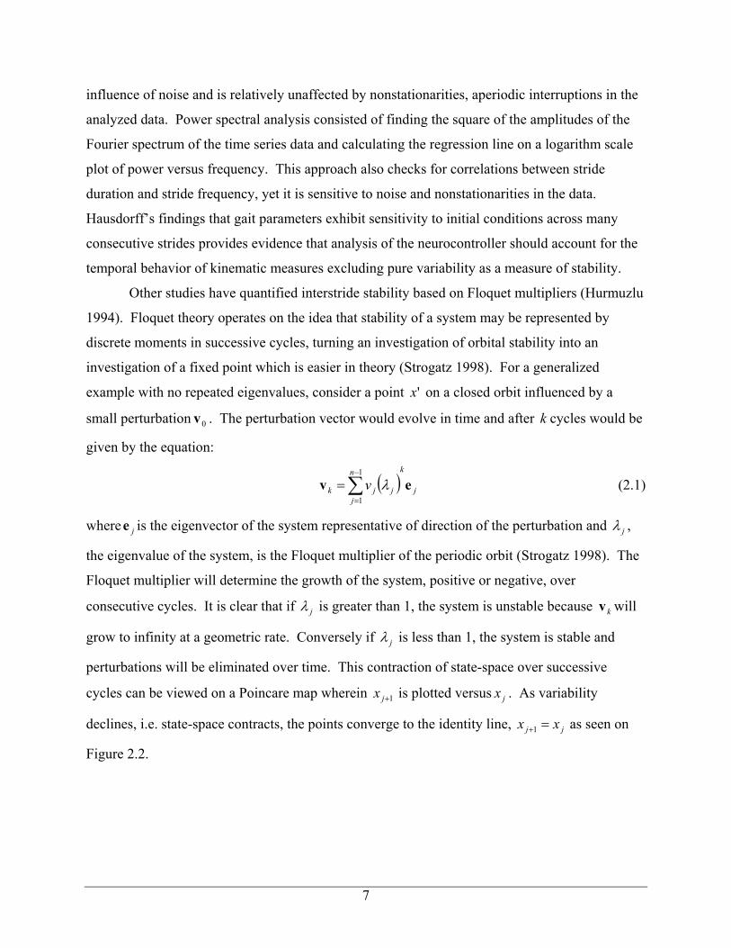
Other studies have quantified interstride stability based on Floquet multipliers (Hurmuzlu

1994). Floquet theory operates on the idea that stability of a system may be represented by

discrete moments in successive cycles, turning an investigation of orbital stability into an

investigation of a fixed point which is easier in theory (Strogatz 1998). For a generalized

example with no repeated eigenvalues, consider a point on a closed orbit influenced by a

small perturbation . The perturbation vector would evolve in time and after cycles would be

given by the equation:

'x

0v k

( ) j

kn

jjjk v ev ∑

−

=

=1

1λ (2.1)

where is the eigenvector of the system representative of direction of the perturbation and je jλ ,

the eigenvalue of the system, is the Floquet multiplier of the periodic orbit (Strogatz 1998). The

Floquet multiplier will determine the growth of the system, positive or negative, over

consecutive cycles. It is clear that if jλ is greater than 1, the system is unstable because will

grow to infinity at a geometric rate. Conversely if

kv

jλ is less than 1, the system is stable and

perturbations will be eliminated over time. This contraction of state-space over successive

cycles can be viewed on a Poincare map wherein is plotted versus . As variability

declines, i.e. state-space contracts, the points converge to the identity line, as seen on

Figure 2.2.

1+jx jx

jj xx =+1

7

Figure 2.2 – A Poincare map demonstrating a stable system

On the Poincare map of a stable system, the smaller the Floquet multiplier, the more rapidly

will approach . Floquet multipliers have the advantage of simultaneously analyzing the entire

dynamics of the system being inspected and being able to definitively answer whether if the

system is stable or unstable. However they are calculated based on the state of the system at a

discrete event in the orbit across successive cycles (N to N+1), thereby ignoring intra-orbit

fluctuations. Other studies have used analogous methods to estimate stability from Poincare

maps, showing small kinematic errors present at the beginning of a walking step were smaller at

the beginning of subsequent steps thereby indicating an attenuation of the kinematic disturbances

through passive or active means (McGeer 1990; Russell 2003). In these models walking stability

was estimated from the contraction rate of kinematic disturbances.

1+jx

jx

Pure variability is a poor quantifier of inter-cycle stability as it has been shown that

control of dynamical biological systems requires temporally based analyses (Dingwell 2001;

Hurmuzlu 1994; McGeer 1990; Russel 2003). Kinematics of dynamic biological system are

continuously disturbed and continual effort is required of neurocontroller to attenuate these

perturbations. Studies have used this attenuation of kinematic variability as a measure of

stability (Hurmuzlu 1994; McGeer 1990; Russel 2003). However, it provides limited insight

regarding intra-stride effects and often ignores kinematic expansion in the time domain, e.g.

stride-duration variance. Effects from a kinematic disturbance can be observed over a time scale

that influences both intra-stride and inter-stride movement (Hausdorff 2001). Consequently,

Lyapunov analyses can be used to track the time-history of individual disturbances recorded

from the time-dependent kinematics (Leipholz 1987).

8

2.2 Lyapunov Analysis

2.2.1 Lyapunov Stability

Stability of a dynamical system may be approximated by its reaction to kinematic

disturbances. A dynamical system’s sensitivity to small kinematic perturbations may be

quantified by the system’s Lyapunov exponents (Rosenstein 1993). One Lyapunov exponent

exists for every dimension, n, of the analyzed trajectory. An n-dimensional sphere of initial

conditions on the analyzed trajectory will evolve in time into an ellipsoid with principal axes

expanding or contracting at rates determined by that axis’ Lyapunov exponent, where n is the

number of state variables. They may be arranged, in order of most rapidly diverging to most

rapidly converging, as λ1 > λ2 > … > λn. For clarity, λ1 may be referred to as λMax as it represents

the largest Lyapunov exponent. Two closely oriented trajectories near an attractor will diverge

at a rate represented by the largest Lyapunov exponent. A helpful visualization can be realized

by noting that the magnitude of the ith principal axis in the Lyapunov spectrum is proportional to

e . The volume spanned by the entire Lyapunov spectrum is then represented by

e

( tiλ )

( )ttt nλλλ +++ L21 (Rosenstein 1993). Rosenstein et al. concluded that when using the full Lyapunov

spectrum a system is stable when the sum of these Lyapunov exponents is negative, i.e. the rate

of convergence is greater than the rate of divergence. The sum of the Lyapunov spectrum must

be less than or equal to zero for the system to be Lyapunov stable, which must also be true for

the existence of an attractor (Rosenstein 1993).

The entire Lyapunov spectrum may be calculated when the equations dictating the

dynamical system are known. When equations are available, measuring expansion or contraction

along the principal axes in the Lyapunov spectrum requires reorthonormalizing these vectors to

maintain a proper phase-space orientation as the system evolves in time. This process of

reorthormalizing vectors guarantees that one vector occurs in the direction of most rapid

expansion. However, since characteristic equations are not typically available for most empirical

systems, calculation of the full Lyapunov spectrum from experimental data is exceedingly

difficult. Calculation of the entire Lyapunov spectrum from empirical data requires finding the

Jacobian matrix representative of system flow for each point on the analyzed trajectory in order

to enable calculation of the evolution of trajectories along the Lyapunov directions.

9

These calculations may be simplified greatly by realizing that two randomly selected

initial trajectories should diverge, on average, at a rate determined by the largest Lyapunov

exponent, λMax (Rosenstein 1993). A randomly selected vector on an attractor will be drawn to

the most unstable manifold due to exponential growth in that direction. This vector will

therefore dominate expansion or contraction along any other Lyapunov direction (Rosenstein

1993). Initially neighboring trajectories or ‘nearest neighbors’ are two points on separates orbits

of the attractor that have the minimum Euclidean distance between the reference point and its

neighbor out of all the points on the attractor. λMax may then be empirically determined from the

divergence of nearest neighbors in a reconstructed n-dimensional state space. Knowing this,

λMax may then be defined by the equation:

( ) tMAXeDtd λ0= (2.2)

where is average Euclidean distance between initially neighboring trajectories at time t and

D

( )td

0 is the initial average distance, d(0).

2.2.2 Reconstructed Dynamics

For a system that is Lyapunov stable, calculation of λMax from experimental data first

requires reconstructing an attractor with enough dimensions to properly capture the dynamics of

the analyzed system. The method of delays is a common and easily implemented method for

reconstructing an n-dimensional state space from scalar data (Packard 1980). The embedding

dimension, n, is chosen as a replacement to the number of state variables in systems where the

characteristic equations are not available and is discussed below (Section 2.2.3). The embedding

dimension must be large enough to allow the full dynamics of the system to be expressed in the

n-dimensional state space. The reconstructed state space may be expressed as a matrix where

each row is a time-vector of a single point of data and each column is an incrementally delayed

version of that vector. The reconstructed attractor, X, is represented by:

( ) ( ) ( ) ( ) ( )[ ]ddd TntxTtxTtxtxtX 1(,,2,, −+++= L (2.3)

where is the original time series data and T( )tx d is the time delay.

A clear example of the method of delays may be applied based to the Lorenz attractor.

The Lorenz attractor is a system of three coupled nonlinear differential equations often used as a

representation of deterministic chaos. The Lorenz equations are as follows:

10

( )( )( )zxyz

yxxzyxyx

βρ

σ

−=−+−=

−=

&

&

&

(2.3)

where σ, ρ, and β are fixed parameters. Figure 2.3 below shows an example of the method of

delays as applied to a Lorenz attractor. Figure 2.3A is the original Lorenz attractor with

coefficients σ = 16.0, ρ = 45.92, and β = 4.0. Figure 2.3B is reconstructed from the X

component of the Lorenz attractor (2.3A) using the method of delays.

Figure 2.3 – A traditional Lorenz attractor (A) and a Lorenz attractor reconstructed using the method of

delays (B)

These plots may appear dissimilar but the Embedding Theorem (Takens 1981) demonstrates that

both curves share the same underlying dynamics, including Lyapunov exponents.

The success of the method of delays in state-space reconstruction is sensitive to the time

delay, Td (Rosenstein 1994). There are several possible approaches for the calculation of Td

which must find an optimal time delay that is neither too large nor too small. In experiments

with noisy finite data, a time delay that is too small will result in a phenomenon known as

redundance while a time delay that is too large will result in irrelevance (Rosenstein 1994).

Redundance is defined as too little information gain in the method of delays. Delayed

coordinates with small time delays are excessively similar to each other, which results in the

reconstructed attractor being compressed along the identity line in the reconstructed state space.

Irrelevance begins to occur when the time delay is larger than about half of mean period of the

signal, thus causing delayed coordinates to become causally unrelated.

11

No consensus exists on which method for the calculation of time delay provides optimal

results. Three popular methods for determining Td include; 1) time delays estimated from the

Averag

2;

s are

t

r

entire data

to

and

sitivity to

f

e Mutual Information function (Dingwell 2000; Fraser 1986), 2) time delays estimated

from the time it takes for the autocorrelation function to drop to a pre-specified fraction of its

initial value (Patla 2003; Rosenstein 1993), and 3) time delays estimated using geometric

approaches based on maximizing some component of the reconstructed state space (Buzug 199

Rosenstein 1994). The average mutual information function finds the amount of shared

information over time delays ranging 1 sample through the entire length of the data set. It

compares a value ( )tx with )( dTtx + for every point in the data set. When the two value

similar, the average mutual information function reports a high value. Td is taken as the firs

minimum of the average mutual information function (Figure 2.4), presuming that this value fo

Td will result in delayed coordinates with minimal redundancy (Dingwell 1998). The

autocorrelation function is similar to the average mutual information function. However

autocorrelation provides a measure of linear dependence on time delay, comparing the

set to time delayed versions of itself (Figure 2.4). The autocorrelation function is thought

work better for linear systems while average mutual information is better applied to nonlinear

systems (Rosenstein 1994). Figure 2.4 below shows the curves generated by autocorrelation

average mutual information function. Also shown in this figure are the reconstructed

representations of a Roux attractor with optimal time delays estimated from autocorrelation and

average mutual information. A Roux attractor is similar to a Lorenz attractor in its sen

initial conditions however it is an example of chemical chaos. Roux attractors prove that strange

attractors like the Lorenz attractor do occur in nature not just mathematics. For a more thorough

description of the nature of Roux attractors see Strogatz 1998 pages 437-440. Time delays in

this figure are selected as the first zero of the autocorrelation function, Td = 24.6 seconds, and the

first minimum of the average mutual information function, Td = 108.2 seconds. The average

mutual information function provides a better time delay for reconstruction in this instance, as

expected since the Roux attractor is nonlinear system. For more information on the specifics o

calculating the average mutual information function, see Fraser and Swinney, “Independent

coordinates for strange attractors from mutual information” (1986).

12

Figure 2.4 – Time delays selected from autocorrelation, C, and the average mutual information function, I,

for a Roux attractor. The attractor reconstructed with time delays from each approach are in the upper

right corner. Picture from Fraser and Swinney 1986, pp. 1135 (Reproduced with author’s permission).

The third method for determining Td is a geometric approach that maximizes the volume

of the reconstructed state space. This approach assumes that stretching the reconstructed

attractor as far as possible leads to the best results in calculating Lyapunov exponents. A

maximum size of the reconstructed attractor will yield the maximum separation between

neighboring trajectories, permitting the best possible resolution when evaluating the distance

between nearest neighbors for calculating Lyapunov exponents (Buzug 1992). While these

approaches provide a good method for eliminating redundance it cannot protect against

irrelevance.

It is critical to determine a time delay that preserves the underlying dynamics of the

analyzed system in state-space reconstruction. For the data we collected, we initially attempted

to calculate Td for each vector of time series data using the average mutual information function.

13

We found however that subtle difference in the signals may lead to drastically different values of

Td for the same measurement between subjects and sometimes differences between right and left

limbs within a subject. Since the method of delays is highly sensitive to Td we chose to calculate

Td by a combination of the average mutual information method and autocorrelation method.

Results from both analyses were compared and Lyapunov exponents were calculated to verify

that these inspected time delays provided acceptable approximations of λMax. The random

outliers of Td created by each method noticeably affected their respective λMax values. Inspection

of data leads us to select time delays as a constant 10 % of the period of each analyzed

movement cycle. Time delays corresponding to 10 % of the cycle length match closely values

found for gait stability analysis (Dingwell in press) of 13 % and 11 % of the stride duration for

analyzing anterior/posterior and superior/inferior motion of a sensor placed over the first thoracic

vertebra.

The number of dimensions utilized in a reconstructed state-space, the embedding

dimension, n, was chosen based on a global false nearest neighbor analysis (Kennel 1993). A

global false nearest neighbor analysis incrementally increases n until the number of false-nearest-

neighbors approaches zero. False nearest neighbors are defined as sets of points that are very

close to each other at dimension n = k but not at n = k+1. An example of a false nearest neighbor

can be seen in Figure 2.5B. When an addition dimension is utilized it is evident that the

trajectory does not actually intersect itself.

Figure 2.5 – Plot of x(t) = sin(2πt) + cos(πt) with embedding dimension n=3 (A) and n=2 (B). Note the

False Nearest Neighbor illustrated by the intersection at [-0.25,0.25] when n=2.

14

A Global False Nearest Neighbor Analysis suggested that an embedding dimension of n = 5 was

appropriate for all the data analyzed in this research. Time delays for the global false nearest

neighbor analysis were based upon the 10 % of cycle length rule discussed above.

2.2.3 Estimation of Maximum Lyapunov Exponent

Once the parameters for state space reconstruction were selected, nearest neighbors

analyses enable time dependent tracking of kinematic variability attenuation. The algorithm

developed by Rosenstein et al. (1993) finds the Euclidian distance between each possible

combination of data points in the time series data set. Each point in the data set is assigned a

nearest neighbor in the n-dimensional reconstructed state-space corresponding to whichever

other point has the minimum Euclidian distance between itself and the reference point. A

constraint is built into this algorithm that nearest neighbors must be separated temporally by a set

window size to guarantee that nearest neighbors occur on separate orbits of the attractor. If

repeated movement cycles were kinematically identical, then a plot of the trajectories would

illustrate each cycle on top of the others in state-space. In this condition, the distance between

nearest neighbors, di(t), would be zero for all pairs of nearest neighbors, i. The distance between

all nearest neighbors is tracked forward in time to record time-dependent change in kinematic

variability.

The rate of change in the distance between nearest neighbors is quantified by the

Lyapunov exponents, λMax, as shown by equation 2.2. The algorithm from Rosenstein et al. finds

the Euclidean distance between all pairs of nearest neighbors. Thus, the distances can be tracked

forward in time for all data points. When one data point of each pair hits the final length of the

data set and is no longer available that nearest neighbor pair is discarded. Analyzed data sets

must be sufficiently long to ensure that λMax may be calculated across a desired time frame

without a significant amount of attrition of nearest neighbor pairs. The logarithm of the

distances between nearest neighbors are averaged at each point in time and outputted as a single

vector of distance. This averaging of all pairs of nearest neighbors at each point in time is key to

enabling calculation of λMax in finite, noisy data sets. λMax is calculated as the slope of the curve

generated by the equation:

( ) ( )idt

iy jln1∆

= (2.4)

15

where is the sampling frequency, t∆ L denotes the average of the contents, and is the

distance between the j

( )id j

th pair of nearest neighbors at time i. λMax was calculated as the slope (via

the least squares “polyfit” command in Matlab) of ( )iy over the range of 0 to 1 complete cycles.

The units of λMax would be represented in terms of measured units (typically degrees for joint

angles) per cycle. To convert these units to distance per second, λMax was divided by average

cycle time for each subject at each velocity condition. Figure 2.6 below shows the calculation of

λMax for the Lorenz attractor Figure 2.3A.

Figure 2.6 – Divergence and λMax for a Lorenz attractor

In calculating the time dependent attenuation of kinematic variability, greater knowledge may be

gained into the behavior of the neurocontroller over traditional variability-based stability

assumptions.

After the stability of the analyzed systems has been investigated, further insight into the

neurocontroller may be investigated by manipulating the signal being analyzed. By normalizing

the length of each movement cycle, temporal variability may be removed, enabling detailed

inspection of how the neurocontroller compensates for spatial differences between cycles

without being influenced by changes in cycle time. Specific sections of movement cycles may

be cut out of larger signals for in depth analysis of key moments in the movement cycle. The

signals being investigated by Lyapunov analysis may be altered in many ways so long as the

modifications are applied uniformly to every cycle in the repetitive task.

16

2.3 Empirical Measurement of System Dynamics

2.3.1 Gait Study Data Collection

Time series analysis on human gait requires data that accurately describes gait dynamics

across many consecutive strides. Human gait has been described by stride length, stride

duration, and double support time but these fail to capture the dynamical nature of gait. Motion

of a sensor placed on the trunk has been used to capture the complexity of the entire body’s

dynamics due to the complex nonlinear coupling between body segments (Dingwell in press).

To permit comparisons of stability between various joints prominent in actuating gait, we

calculated joint angles for the right and left hip, knee, and ankle. Lower-body kinematic data

were recorded from 21 reflective markers using a 6-camera, 3-D, video motion analysis system

(Vicon, Oxford Metrics). Markers were placed on the sacrum, and symmetrically across the

sagittal plane on the anterior superior iliac spine (ASIS), posterior superior iliac spine (PSIS),

anterior thigh, lateral epicondyle of the femur, anterior shin, lateral malleolus of the fibula,

dorsum of the foot, 5th metatarsal, calcaneous and hallux. Joint angles were calculated based on

the definition of a dot product:

θcosBABA =•→→

(2.5)

where and →

A→

B are vectors defining limbs and θ is the bounded joint angle. Limb vectors for

the foot, leg, thigh, and trunk are defined as the vector between the lateral malleolus and 5th

metatarsal, lateral malleolus and lateral epicondyle of the femur, lateral epicondyle of the femur

and hip joint center (HJC), and posterior superior iliac spine and anterior superior iliac spine.

The HJC was calculated based on anthropometrics to find the center of rotation of the hip with

respect to nearby markers. The HJCs were determined from the equations provided by Vicon

(Oxford Metrics) for use in their Golem model:

( ) FSCHJCx += θsin (2.6)

( ) ( ) ( )ββθ cos)(sincos dDCHJCy +−= (2.7)

( ) ( ) ( )ββθ sin)(coscos dDCHJCz +−= (2.8)

where S is dependent on the side of the body, 1 for right, -1 for left, F is half of the distance

between the right and left ASIS, θ is fixed at 28.4 degrees, β is set at 18 degrees, d is the marker

radius, 14.5 mm, and C and D are given by equations 2.8 and 2.9 repectively.

( ) 0153.0115.0 −= LC (2.9)

17

( ) 04856.01288.0 −= LD (2.10)

In equations 2.8 and 2.9, L is the average leg length, the sum of the distance between the ASIS

and lateral epicondyle of the femur and the lateral epicondyl of the femur and the lateral

malleolus. The coordinates of the HJC are rotated with the pelvis and added to coordinate

corresponding to the front of the pelvis determined as the midpoint of the line segment between

the right and left ASIS.

To properly scale walking velocity to leg length, subjects walked as set percentages of

their Froude Velocity, VF. VF is derived by looking at gait as a simple inverted pendulum. A

free body diagram of this inverted pendulum model may be seen in Figure 2.7 below.

Figure 2.7 – Free body diagram of the inverted pendulum model

The maximum theoretically possible walking velocity occurs at the velocity at which upward

centripetal force equally balances weight. Based on this scenario, VF is calculated so that weight

is counteracted by vertical force due to radial acceleration.

RVmmg F

2

= (2.11)

Solving for VF gives the equation for normalizing velocity to a subject.

gRVF = (2.12)

Froude velocity was originally derived as a scaling factor to calculate the dynamic similarity of

full size ships with more manageable models however it has found applications in a widespread

array of investigations into locomotion (Vaughan 2005). VF has been used as a scaling factor to

enable comparisons of human gait with geometrically similar gait patterns in animals and robots

(Alexander 1984). VF also may be applied to check for dynamic similarities between humans of

18

different sizes and ages (Vaughan 2003). VF even helps explain the difficulties that astronauts

faced in trying to walk on the Moon at gait velocities comfortable to humans on Earth (Minetti

1998; Cavagna 2000). Other studies analyzing gait at varying velocities have used percentages

of preferred walking speed (PWS) as the independent variable. Typical preferred walking speed

occurs at approximately 0.45 % VF and analyzed walking speeds typically spanned 60 % - 140 %

PWS, which corresponds approximately to 30 % - 60 % VF (Dingwell in press). This range of

walking speeds may be more common during healthy walking than velocities at 20 % and 80 %

VF however they fail to inspect the response of the neurocontroller to velocities above and below

this relatively comfortable zone.

2.3.2 Back Study Data Collection

To the best of the author’s knowledge, time series analysis of kinematic data detailing

cyclic motions of the trunk has never been attempted. Studies have shown that injuries often

occur during repetitive lifting tasks (NIOSH, 1999; Marras 1993). The goal of this study was to

investigate dynamic stability of the trunk as influenced by speed and symmetry. Magnetic

sensors reporting position and rotation were placed on the palm of the right hand, manubrium of

the sternum, tenth thoracic and first sacral vertebrae. Originally it was hoped to compare

stability of the trunk markers to stability of the palm marker to investigate any possible

compensatory behavior in which the trajectory of the hands may possibly be more stable than

any trunk motions in the presence of increased speed or asymmetry.

Participating subjects performed motions corresponding to pure flexion pure twist, and

asymmetric flexions which included twists to the right for one trial, left for another. Subjects

were asked to touch targets with their hands; hands together, fingers intertwined. Targets were

placed at pre-specified locations similar to methods described by Thomas (2003). An upper

target was placed at shoulder height in the anterior sagittal midline such that it could be

contacted while standing upright with arms outstretched parallel to the ground. A lower target

was placed in the sagittal midline 50 cm anterior to the knee. Subjects were asked to touch the

upper target followed by the lower target sequentially with contact occurring at the beats of the

metronome for the duration of each experimental trial. Asymmetric trials were recorded wherein

the upper target was moved to one side and the lower target to the opposing side as to induce an

approximately 450 axial rotation of the torso at the upper and lower targets. Positions of the

19

upper and lower targets were mirrored about the sagittal plane in another trial and results

averaged to avoid any influence of dominant sides of the subject’s body.

A metronome was used to dictate the pace at which subjects moved for slow and fast

trials. The full cycle of motion took 2 full beats of the metronome to complete. For fast trials

the metronome was set to 80 beats per minute (40 cycles per minute) while slow trials took place

at 40 beats per minute (20 cycles per minute). Subjects were given time to practice these

movements until they were comfortable with the movement trajectory and movement pace.

Once comfortable with the motions, position and rotation data of the magnetic sensors were

recorded for 30 consecutive trials. Subjects were given two minutes rest between data

collections to minimize fatigue influence on results. The order of motions was randomized to

avoid any influence from potentially remaining effects of fatigue or learned-behavior.

Angle data of each magnetic sensor was reported as euler angle rotations about the Z, Y’,

X’’ axes. The Z axis corresponds to positive vertical direction with rotations about this axis

equating to twisting of the trunk. The Y’ axis is collinear with the vector pointing laterally to the

subject’s right side after being rotated around the Z axis. Rotations about this axis equate to

trunk flexion/extension and are the primary concern of this section of study. The X’’ axis points

anteriorly out of the trunk. There were no significant motions about this axis in this study.

While data was collected on 30 healthy subjects, equipment problems nullified results of

10 subjects. For Lyapunov analysis, rotational data must be represented as continuous data. Due

to some unknown error during data collection, discontinuities were present and irreparable in the

trunk flexion/extension data for 10 subjects. This may potentially be prevented in future studies

by either more carefully selecting which axes are being rotated about or by using 3-D video

motion analysis in place of electromagnetic motion sensors.

2.4 References

Hausdorff JM, Rios DA, Edelberg, MD. Gait variability and fall risk in community-living older adults: A 1-year prospective study. Archives of Physical Medicine and Rehabilitation. 2001; 82: 1050-1056. Dingwell JB, Cusumano JP. Nonlinear time series analysis of normal and pathological human walking. Chaos. 2000; 10(4): 848-863. Survey of Occupational Injuries and Illnesses, National Institute of Occupational Safety and Health. 1999, Washington, DC.

20

Marras WS, and Mirka GA. Electromyographic studies of the lumbar trunk musculature during the generation of low-level trunk acceleration. Mirka G.A. 1993;11: 811-817. Panjabi MM. The stabilizing system of the spine. Part I Function, dysfunction, adaptation and enhancement. Journal of Spinal Disorders 1992; 5: 383-389. Englander F, Hodson TJ, Terregrossa RA. Economic dimensions of slip and fall injuries. Journal of Forensic Science. 1996; 41(5): 733-746. Luo X, Pietrobon R, Sun SX, Liu GG, and Hey L. Estimates and patterns of direct health care expenditures among individuals with back pain in the United States. Spine 2004;29:79-86. Alexander NB. Gait disorders in older adults. Journal of the American Geriatric Society. 1996; 44: 434-351. Cavanagh PR, Derr JA, Ulbrecht JS, Maser RE, Orchard TJ. Problems with gait and posture in neuropathic patients with insulin-dependent diabetes mellitus. Diabetic Medicine 1992;9:469-474. Strogatz SH. Nonlinear dynamics and chaos. Addison-Wesley Publishing Company, New York 1998; pp. 128-130,141-142,196-197,281-282,317-325,437-440. Leipholz H. Stability Theory. An introduction to the stability of dynamic systems and rigid bodies. New York: John Wiley & Sons, 1987. Dingwell JB, Cusumano JP, Sternad D, and Cavanagh PR. Beyond 3D: A nonlinear dynamics approach to the analysis of human locomotion. Proceedings of the 5th International Symposium on 3D Analysis of Human Movement, Chattanooga, TN, July, 1998, pp. 140-143. Öberg T, Karsnia A, and Öberg K. Basic gait parameters: Reference for normal subjects, 10-79 years of age. Journal of Rehabilitation Research and Development, 1993; 30(2): 210-223 Hausdorff JM, Peng CK, Ladin Z, Wei JY, and Goldberger AL. Is walking a random walk? Evidence for long-range correlations in stride interval of human gait. J.Applied Phys. 1995; 78: 349-358. Maki BE. Gait changes in older adults: Predictors of falls or indicators of fear? Journal of the American Geriatric Society. 1997; 45(3): 313-320. Dingwell JB, Cusumano JP, Cavanagh PR, and Sternad D. Local dynamic stability versus kinematic variability of continuous overground and treadmill walking. J Biomech. Eng. 2001; 123: 27-32.

Buzzi U H, Stergiou N, Kurz MJ, Hageman PA, and Heidel J. Nonlinear dynamics indicates aging affects variability during gait. Clinical Biomechanics. 2003; 18: 435-443.

21

Goswami A, Espiau B, and Thuilot B. A study of passive gait of a compas-like biped robot: Symmetry and Chaos. Intl.J.Robot.Res. 1998; 17: 1282-301. Hurmuzlu Y, and Basdogan C. On the measurement of dynamic stability of human locomotion. J.Biomech.Eng. 1994; 116: 30-36. Owings TM, and Grabiner MD. Variability of step kinematics in young and older adults. Gait and Posture. 2004; 20(1): 26-29. McGeer T. Passive dynamic walking. International Journal of Robotics Research. 1990; 9(2): 62-82. Russell S, Granata KP, and Sheth P. Virtual slope control of a forward dynamic bipedal walker. J Biomech.Eng 2005;127:114-122.. Hurmuzlu Y, Basdogan C, and Carollo JJ. Presenting joint kinematics of human locomotion using phase plane portraits and Poincare maps. J.Biomechanics 1994; 27: 1495-1499. Rosenstein MT, Collins JJ, and De Luca CJ. A Practical method for calculating largest Lyapunov exponents from small data sets. Physica D. 1993;65:117-134. Packard NH, Crutchfield JP, Farmer JD, and Shaw RS. Geometry from a time series. Physical Review Letters. 1980;45:712-716. Takens F. Detecting Strange Attractors in Turbulence. In: Young LS. ed. Dynamical Systems and Turbulence. New York: Springer, 1981:366-81. Rosenstein MT, Collins JJ, and De Luca CJ. Reconstruction expansion as a geometry-based framework for choosing proper delay times. Physica D. 1994;73:82-98. Fraser AM, and Swinney HL. Independent coordinates for strange attractors from mutual information. Physical Review A. 1986; 33(2): 1134-1140. Patla AE. Strategies for dynamic stability during adaptive human locomotion. IEEE Engineering in Medicine and Biology Magazine 2003; 22: 48-52. Buzug T, and Pfister G. Optimal delay time and embedding dimension for delay-time coordinates by analysis of the global static and local dynamic behavior of strange attractors. Physical Review A. 1992; 45(10): 7073-7084. Dingwell JB, Marin LC. Kinematic variability and local dynamic stability of upper body motions when walking at different speeds. J Biomech. 2004; In Press. Kennel MB, Brown R, Abarbanel HDI. Determining minimum embedding dimension using a geometrical construction. Physical Review A. 1992; 45(A): 3403-3411.

22

Vaughan CL and O’Malley MJ. Froude and the contribution of naval architecture to our understanding of bipedal locomotion. Gait and Posture. 2005; 21: 350-362. Alexander RM. The gaits of bipedal and quadrupedal animals. International Journal of Robotics Research. 1984;3(2):49-59. Minetti AE. The biomechanics of skipping gaits: a third locomotion paradigm. Proceedings of the Royal Society of London. 1998;265:1227-1235. Cavagna GA, Willems PA, Heglund NC. The role of gravity in human walking: pendular energy exchange, external work and optimal speed. Journal of Physiology. 2000;528: 657-668. Thomas JS, Corcos DM, and Hasan Z. Effect of movement speed on limb segment motions for reaching from a standing position. Exp.Brain Res. 2003;148:377-387. Vaughan CL, Langerak NG, and O'Malley MJ. Neuromaturation of human locomotion revealed by non-dimensional scaling. Exp.Brain Res. 2003;153:123-127. Fraser AM, and Swinney HL. Independent coordinates for strange attractors from mutual information. Physical Review A. 1986; 33(2): 1134-1140.

23

Submitted to: Gait & Posture 29 August 2005 ORIGINAL

The Influence of Gait Speed on Local Dynamic Stability

Scott A England

Kevin P. Granata, Ph.D

Musculoskeletal Biomechanics Laboratories Department of Engineering Science & Mechanics

School of Biomedical Engineering & Science Virginia Polytechnic Institute & State University

219 Norris Hall (0219) Blacksburg, VA 24061

Address all correspondence to: K.P. Granata, Ph.D.

Musculoskeletal Biomechanics Laboratories Department of Engineering Science & Mechanics Virginia Polytechnic Institute & State University 219 Norris Hall (0219) Blacksburg, VA 24061 Granata@VT.edu

Keywords : Gait, Stability, Walking velocity

24

Abstract:

The focus of this study was to examine the role of walking velocity in stability during

normal gait. Local dynamic stability was quantified through the use of maximum finite-time

Lyapunov exponents, λMax. These quantify the rate of attenuation of neighboring kinematic

trajectories of joint angle data recorded as subjects walked on a motorized treadmill at 20, 40, 60,

and 80 percent of the Froude Velocity. A monotonic trend between λMax and walking velocity

was observed with increased λMax at faster walking velocities. This trend was evident whether

temporal variability remained or was removed from the data. This suggests that slower walking

velocities lead to increases in stability. These results may reveal more detailed information on

the behavior of the neuro-controller than variability based analyses alone.

25

3.1 Introduction

Stability is a critical component of walking 8;13. It can be defined as the ability to

maintain functional locomotion despite the presence of small kinematic disturbances or control

errors. Stability of standing static postures is often recorded from kinematic variability

associated with the center-of-pressure under the equilibrium base of support. However, walking

is a dynamic condition wherein the joint control torques change with time and posture thereby

requiring that stability must be determined from state- and time-dependent variability14. In other

words, stability of walking requires analyses that account for both time and movement.

Kinematics of walking and associated variability are influenced by walking velocity thereby

indicating potential velocity effects on stability 15;18. Some studies suggest that one possible

motivation for slower walking speed in the elderly and in individuals with joint disease and

neuropathology is to improve stability4. This assumes that stability of walking is improved at

slower velocities. The purpose of this study was to test this assumption.

Stability of dynamic systems can be estimated from nonlinear analyses of kinematic

variability3. Others have quantified the magnitude of kinematic variability as an estimate of

stability wherein increased variability was assumed to correspond to decreased stability 10;25.

However, measurements of kinematic variability are subtly different than stability. It is

reasonable to assume that every walking stride could be similar to every other stride. Natural

kinematic variance observed in empirical data is therefore attributed to mechanical disturbances

or control errors. These disturbances are attenuated in time by the neuro-controller and

musculoskeletal system in order to maintain a stable walking pattern. Thus, it is reasonable to

estimate stability from the time-dependent expansion or attenuation of kinematic variability 8;13.

The magnitude of kinematic variability is influenced by external disturbances whereas the time-

history of the movement following the disturbance is primarily a function of stabilizing

neuromuscular control.

Techniques for quantifying dynamic stability were largely developed from biomechanical

models of bipedal gait. Miura and Shimoyama implemented a bipedal model of gait with an

open-loop control scheme using “joint torque schedules” that were executed at predetermined

time events in the gait cycle17. Their gait was unstable and would fail without active feedback

corrections necessary to attenuate movement errors and perpetuate motion. McGeer

26

demonstrated that a stable, periodic motion can be achieved by a passive, knee-less model

walking down a slope16. After several steps the simulation settled into a steady-state walking

pattern matched to the slope of the hill. Stability was estimated by Poincare maps to demonstrate

that small kinematic errors introduced at the beginning of a step were attenuated when measured

in subsequent steps. A similar model by Russell et al 23 implemented an active feedback

controller to attenuate kinematic errors so as to achieve stable bipedal walking on level ground.

In these models walking stability was estimated from the contraction rate of kinematic

disturbances. The rate of kinematic error attenuation can also been used as an empirical measure

of stability in human gait12.

Stability of human walking can be estimated from temporal analyses of multi-

dimensional variability. Disturbance to the walking trajectory is an ongoing process so the

attenuation of kinematic variability is continually manifest. Poincare maps quantify the

attenuation of kinematic variability between consecutive strides13. This method has the

advantage of measuring stability in a multi-degree-of-freedom system. However, it provides

limited insight regarding intra-stride effects and often ignores expansion in temporal variability,

e.g. stride-duration variance. Effects from a kinematic disturbance can be observed over a time

scale that influences both intra-stride and inter-stride movement10. Dynamic analyses can be

used to track the time-history of individual disturbances recorded from the time-dependent

kinematics14. The time-dependent rate of kinematic expansion is measured by the Lyapunov

exponent, λ. One Lyapunov exponent exists for every movement dimension of the analyzed

kinematic trajectory. These can be arranged, in order of most rapidly diverging to most rapidly

converging, as λ1 > λ2 > … > λn. To avoid confusion, λ1 may be referred to as λMax to represent

the largest Lyapunov exponent. Rosenstein et al. concluded that when using the full Lyapunov

spectrum, a system is stable when the sum of these Lyapunov exponents is negative, i.e. the rate

of convergence is greater than the rate of divergence21. Calculation of the full Lyapunov

spectrum from experimental data however, is exceedingly difficult. These calculations may be

simplified greatly by realizing that two randomly selected initial trajectories should diverge, on

average, at a rate determined by the largest Lyapunov exponent, λMax. Calculation of λMax is

relatively easy and can be used to evaluate the influence of walking velocity on dynamic stability

of walking.

27

The goal of this study was to 1) implement Lyapunov analyses to characterize stability of

dynamic steady-state walking, and 2) test whether walking velocity influences stability of

walking. This is the first in a series of studies planned to quantify the stability of gait in normal-

developing subjects and patients with developmental neuro-impairment.

28

3.2 Methods

3.2.1 Experimental Procedures.

Kinematic data were recorded from 19 healthy adult subjects including 6 male and 13

females; mean age (± standard deviation) 22.5 ± 2.8 yr; mean height 1.7 ± 0.1 m and mean

weight 65.7 ± 12.7 kg. Lower-body kinematic data were recorded from 21 reflective markers

using a 6-camera, 3-D, video motion analysis system (Vicon, Oxford Metrics). Markers were

placed on the sacrum, anterior superior iliac spine, posterior superior iliac spine, anterior thigh,

lateral epicondyle of the femur, anterior shin, lateral malleolus of the fibula, dorsum of the foot,

5th metatarsal, calcaneous and hallux. Subjects walked barefoot on a treadmill at 20, 40, 60 and

80 percent of their Froude velocity, VF. Walking velocity was expressed in terms of Froude

velocity to appropriately scale the walking speed to leg length and pendulum dynamics24. Each

subject’s Froude Velocity was calculated based on the equation:

gRVF ∗= (3.1)

where R is the distance between the greater trochanter and lateral malleolus of the fibula and g is

the acceleration due to gravity. Comfortable walking speed is typically 0.45 VF and running is

initiated at 1.0 VF.

Four repeated collections of 30 walking strides per velocity condition were recorded for

each subject. Ankle, knee and hip angles were calculated from the 3-D locations of the marker

set using standard techniques (MATLAB, Mathworks, Inc., Natick, MA). Analyses were limited

to the plantarflexion / dorsiflexion dimension of the ankle, knee flexion angle and hip flexion

angle. Previous studies recommend against filtering the data before Lyapunov analyses so as to

retain spatio-temporal fluctuations and nonlinearities6. However, we believe that kinematic

signals at frequencies greater than 10 Hz are unlikely related to the musculoskeletal motion and

therefore filtered the data with a 10 Hz, low-pass 2nd-order Butterworth filter. Regardless of this

difference in opinion regarding filtering the results were similar between these studies.

Since cadence changes with walking velocity but data sampling frequency remained

fixed, a dilemma arises with respect to the proper way to compare data collected at different

walking velocities. Specifically, since stride-duration decreases with walking velocity, data

collected at 80% VF would likely have less than half as many data points per stride, on average,

29

as data collected at 20% VF. Data were time-normalized in two separate manners and results

compared. First, every stride was time-normalized to 100 data points per stride. This provides

an equal number of data points per stride regardless of velocity but it removes stride-to-stride

temporal variations that are an important component of Lyapunov stability analyses. Second,

data sets of 30 contiguous strides were re-sampled to be 3000 data points long, i.e. approximately

100 data points per stride on average but any individual stride could be greater than or less than

100 data points. This permits stride-to-stride temporal variation while normalizing the data such

that the average number of data points per stride were similar for each velocity condition. In an

attempt to understand the influence of re-sampling frequency on the Lyapunov analysis, the same

data were also analyzed with data re-sampled to 1500 data points. Independent stability analyses

were performed on each time-dependent joint angle, xj(t), where j=1:6 was the joint number and t

was the re-sampled time interval.

3.2.2 Calculating Dynamic Stability.

Local dynamic stability was determined based on the maximum finite-time Lyapunov

exponent, λMax. These were used to quantify the exponential attenuation of variability between

neighboring kinematic trajectories. The approach assumes that every stride could be identical to

every other stride. Stride-to-stride differences in kinematic measurements are attributed to small

perturbations. Therefore, kinematic variability can be used to evaluate the stability of the system

by tracking the progression of a perturbed gait cycle back to the mean. Since the recorded time-

series data, xj(t), are one dimensional column vectors of joint angles it was necessary to

reconstruct an n-dimensional state-space out of the kinematic data in order to accurately

determine dynamic perturbations to the ideal gait cycle. One typical method of creating an n-

dimensional state-space from scalar data is by method of delays. Using this method a joint angle

in n-dimensional space would appear as:

Yj(t) = [xj(t), xj(t+Td), xj(t+2Td). . . xj(t+(n-1)Td)] (3.2)

where xj(t) is the original scalar data of joint angle and Td is a constant time delay. A

reconstructed state-space Yj(t) with an embedding dimension of n = 3 can be seen in Figure

3.1A.

30

Figure 3.1. (A) Reconstructed state-space kinematics of knee angle with 3 embedded dimensions. (B)

Divergence of nearest neighbors with temporal variability permitted

The success of state-space reconstruction by the method of delays is sensitive to the time

delay, Td22. Several methods exist for calculation of Td. There is no consensus on which method

provides optimal results. Three methods have been popularized including; 1) time delays

estimated from the Average Mutual Information function 4;7, 2) time delays estimated from the

time it takes for the autocorrelation function to drop to a pre-specified fraction of its initial

value19, and 3) time delays estimated using geometric approaches based on maximizing some

component of the reconstructed state space 2;22. Using the Average Mutual Information function

and the autocorrelation approach, we observed time-delay estimates ranging from 9 to 40

samples. To assure that all of the trials were analyzed similarly, a constant Td of 10 samples (10

percent of the length of the gait cycle) was used for all reconstructed state space.

The number of state-space dimensions, n in equation 1, is selected based on a Global

False-Nearest-Neighbor Analysis21. This method incrementally increases n until the number of

false-nearest-neighbors approaches zero. False nearest neighbors are defined as sets of points

31

that are very close to each other at dimension n = k but not at n = k+1. For example, a plot of

x(t) = sin(2πt) + cos(πt) with n = 3 embedding dimensions in Figure 3.2A illustrates that the

curve does not intersect itself. When this same data is viewed in two-dimensions, n = 2, it

artificially appears to cross-over itself, i.e. a false nearest neighbor would occur at the crossover

point as in Figure 3.2B.

Figure 3.2. Plot of x(t) = sin(2πt) + cos(πt) with embedding dimension n=3 (A) and n=2 (B). Note the

False Nearest Neighbor illustrated by the intersection at [-0.25,0.25] when n=2.

A Global False Nearest Neighbor Analysis suggested that an embedding dimension of n = 5 was

appropriate for the analyzed data.

Maximum finite-time Lyapunov exponents were calculated based on the algorithm

published by Rosenstein et al21. The Euclidean distance between nearest neighbors, di(t), was

computed for each data-point, i, in the reconstructed state-space Yj(t) for all time, t. Nearest

neighbors are found by selecting data points from separate cycles that are closest to each other in

reconstructed state-space. If repeated strides were kinematically identical, then a plot of the

trajectories would illustrate each cycle on top of the others in state-space. In this condition, the

distance between nearest neighbors, di(t), would be zero for all pairs of nearest neighbors, i.

However, in the empirically measured data the distance between nearest neighbors, di(t), was

32

greater than zero as in Figure 3.1A. Hence, there are clearly kinematic disturbances observable

in the data. The distance between all nearest neighbors was tracked forward in time to record

time-dependent changes in kinematic variability as in Figure 3.1B. The rate of change in the

distance between nearest neighbors is quantified by the Lyapunov exponents, λ,

( ) teDtd λ0= (3.3)

where D0 is the average displacement between trajectories at t = 0. Two randomly selected

initial trajectories should diverge, on average, at a rate determined by the largest Lyapunov

exponent, λMax 21. Therefore, the maximum Lyapunov exponent, λMax was approximated from

the experimental joint-angle data as the slope of the linear best-fit line to the curve created by the

equation:

( ) ( )kdt

ky iln1∆

= (3.4)

where ( )kdiln represents the average logarithm of displacement for all pairs of nearest

neighbors, i. The maximum finite-time Lyapunov exponent, λMax, was calculated as the slope of

the logarithm of the average divergence across the span of 0 to 1 strides as shown in Figure 3.3.

Figure 3.3. Average logarithmic divergence vs time. The slope of the logarithmic relation from 0 to 1

stride represents λMax.

33

A value of λMax was computed for each joint of every subject at each walking velocity. λMax was

interpreted as a measure of dynamic stability.

Statistical analyses were performed to determine the effects of walking velocity on

stability. Lyapunov exponents were computed independently for the ankle, knee and hip for

each subject and each walking velocity, VF = 20, 40, 60, 80%. Preliminary analyses revealed no

statistically significant differences in stability between the right and left limbs. Therefore, data

from the right and left limbs were pooled for statistical analyses. Two-factor repeated measures

analysis of variance (ANOVA) tested the within-subject effects of joint and walking velocity on

λMax. Analyses were performed using commercial software (Statistica, 4.5 Statsoft, Inc., Tulsa

OK) using a significance level of α < 0.05.

34

3.3 Results

When the full 30 stride data sets at each velocity were re-sampled to be 3000 data points

in duration, variability in stride-duration was observed despite walking at constant velocity.

Mean and standard deviations of stride time were 1.57±0.062 seconds at 20% VF, and

1.12±0.021, 0.94±0.012, and 0.79±0.016 seconds for 40, 60, and 80% VF respectively. This

stride-time variability was significantly higher (p<0.001) at 20% VF than at 40, 60, and 80% VF.

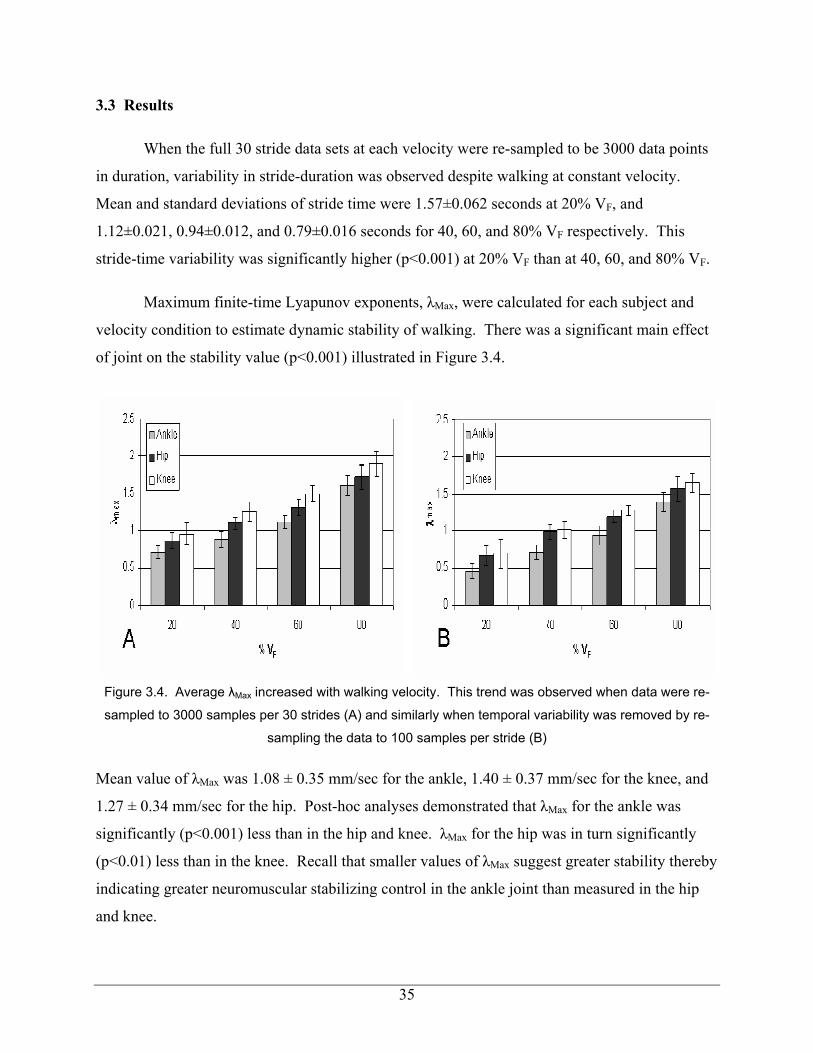
Maximum finite-time Lyapunov exponents, λMax, were calculated for each subject and

velocity condition to estimate dynamic stability of walking. There was a significant main effect

of joint on the stability value (p<0.001) illustrated in Figure 3.4.

Figure 3.4. Average λMax increased with walking velocity. This trend was observed when data were re-

sampled to 3000 samples per 30 strides (A) and similarly when temporal variability was removed by re-

sampling the data to 100 samples per stride (B)

Mean value of λMax was 1.08 ± 0.35 mm/sec for the ankle, 1.40 ± 0.37 mm/sec for the knee, and

1.27 ± 0.34 mm/sec for the hip. Post-hoc analyses demonstrated that λMax for the ankle was

significantly (p<0.001) less than in the hip and knee. λMax for the hip was in turn significantly

(p<0.01) less than in the knee. Recall that smaller values of λMax suggest greater stability thereby

indicating greater neuromuscular stabilizing control in the ankle joint than measured in the hip

and knee.

35

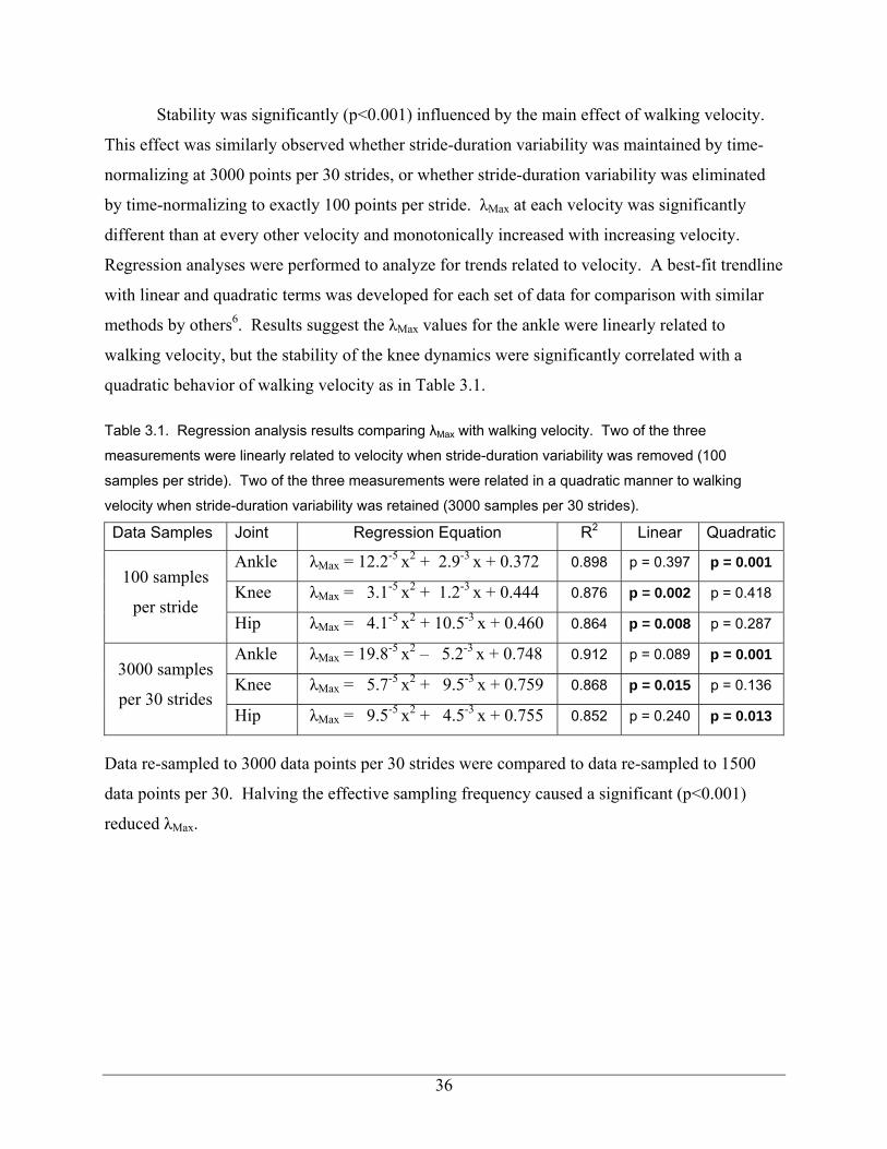
Stability was significantly (p<0.001) influenced by the main effect of walking velocity.

This effect was similarly observed whether stride-duration variability was maintained by time-

normalizing at 3000 points per 30 strides, or whether stride-duration variability was eliminated

by time-normalizing to exactly 100 points per stride. λMax at each velocity was significantly

different than at every other velocity and monotonically increased with increasing velocity.

Regression analyses were performed to analyze for trends related to velocity. A best-fit trendline

with linear and quadratic terms was developed for each set of data for comparison with similar

methods by others6. Results suggest the λMax values for the ankle were linearly related to

walking velocity, but the stability of the knee dynamics were significantly correlated with a

quadratic behavior of walking velocity as in Table 3.1.

Table 3.1. Regression analysis results comparing λMax with walking velocity. Two of the three

measurements were linearly related to velocity when stride-duration variability was removed (100

samples per stride). Two of the three measurements were related in a quadratic manner to walking

velocity when stride-duration variability was retained (3000 samples per 30 strides).

Data Samples Joint Regression Equation R2 Linear Quadratic

Ankle λMax = 12.2-5 x2 + 2.9-3 x + 0.372 0.898 p = 0.397 p = 0.001

Knee λMax = 3.1-5 x2 + 1.2-3 x + 0.444 0.876 p = 0.002 p = 0.418 100 samples

per stride Hip λMax = 4.1-5 x2 + 10.5-3 x + 0.460 0.864 p = 0.008 p = 0.287

Ankle λMax = 19.8-5 x2 – 5.2-3 x + 0.748 0.912 p = 0.089 p = 0.001

Knee λMax = 5.7-5 x2 + 9.5-3 x + 0.759 0.868 p = 0.015 p = 0.136 3000 samples

per 30 strides Hip λMax = 9.5-5 x2 + 4.5-3 x + 0.755 0.852 p = 0.240 p = 0.013

Data re-sampled to 3000 data points per 30 strides were compared to data re-sampled to 1500

data points per 30. Halving the effective sampling frequency caused a significant (p<0.001)

reduced λMax.

36

3.4 Discussion

It has been suggested that individuals with impaired neuromuscular control may walk

with reduced velocity in order to improve their stability4. Existing evidence reveals that

kinematic and spatio-temporal variability are influenced by walking velocity18. However,

stability might be poorly represented by the magnitude of variability5. Instead, assessment of

stability may require examination of how the neuro-control system handles kinematic variability,

i.e. the active and passive control of disturbances. Therefore, the goal of the current study was to

determine the relationship between walking velocity and the Lyapunov exponent that represents

the time-dependent change in joint angle variability. Dingwell and Martin6 recently reported

results from a similar study to investigate the influence of walking velocity on stability . They

observed that kinematic variability demonstrated a quadratic behavior, i.e. variability was least

near the comfortable walking velocity but it was increased at both slow and fast walking

velocities. Conversely, their analyses suggest that stability increased linearly with walking

velocity. Our analyses agree with this monotonic trend the relation was not necessarily linear.

Lyapunov analyses revealed that stability was significantly influenced by walking

velocity. When the data from every stride were time-normalized to 100 data points per stride, a

linear relationship was observed between λMax and velocity. Smaller λMax represents a more

stable system. Therefore, every joint was significantly more stable lower velocities. These

results agree with the conclusions of Dingwell and Martin6 despite differences in measurement

techniques and processing. However, this method of time-normalizing the data artificially

removes stride-to-stride temporal variations. A kinematic disturbance can influence not only the

movement pattern but it can also influence the time duration of the movement trajectory. To

accommodate stride-duration variability separate analyses were performed wherein the data from

30 strides were time-normalized to 3000 data points in total. This process causes a mean stride-

duration of 100 points per cycle but all strides were not necessarily of equal length. In fact,

results demonstrate mean stride-to-stride variation of 2.3 percent. Using this time-normalizing

procedure walking velocity continued to significantly influence the Lyapunov exponent, λMax,

i.e. monotonic trend of lower stability at faster walking velocities. Unlike the analyses with

exactly 100 points per stride, the temporal variation introduces a more quadratic trend.

37

Fast walking velocity may influence dynamic stability by a combination of several

mechanisms. Walking velocity affects kinematic double-support time, step width and other

clinical correlates of stable walking1. Modified support mechanics may influence the ability to

control movement disturbances. Analyses of bipedal walking demonstrate the existence of a

biomechanical resonance associated the pendulum-like behavior of the skeletal structure and

muscle stiffness11. These may contribute to stability at the preferred walking velocity16.

Therefore, walking at velocities that are faster or slower than this resonant frequency require

greater active neuromuscular control to maintain stable periodic movement20. In other words,

faster walking velocities increase the segmental momentum thereby requiring greater effort from

the neuro-controller to attenuate kinematic disturbances. Short stride durations limit the

allowable time for neuromuscular corrections to compensate for mechanical disturbances or

controller errors. Slow walking velocities require active control that is out-of-phase with

movement to slow the natural dynamics of the passive system. Hence, most of the variability

observed during slow walking velocities appeared to be attributable to fluctuations in stride

duration whereas during fast walking the variability was primarily associated with kinematic

disturbances. This suggests that these subjects may be temporally less stable at slower walking

velocities than at fast walking velocities but spatially more stable at slow velocities.

Nonetheless, results suggest that the neuro-control system more effectively controlled kinematic

disturbances at slow velocities than during fast walking.

Data processing and analyses techniques must be considered when interpreting the

results. Rosenstein et al21 observed that Lyapunov analyses are sensitive to the sampling

frequency and length of the data set. If the sampling frequency is sufficient to characterize the

kinematic variance then the length of the data set is more critical than sampling frequency. In

the measured data, mean stride duration at 80% VF was 0.79 ± 0.03 seconds whereas at 20% VF

it was 1.57 ± 0.11 seconds. If one were to use a common sampling rate for all velocities, then

the length of the data set at fast walking velocities would include approximately half the number

of data samples per stride when compared to slow walking velocities. The only other study that

directly compared walking velocity to dynamic stability compared three minutes of gait data

collected between 60 % and 140 % of a subject’s preferred walking speed6. In that study, a fast

trial may potentially have more than twice as many strides with half as many data points per

stride compared to a slow walking trial, i.e. greater sample density at slow velocities than at fast

38

velocities. To investigate the effect of halving the number of data samples per stride, we

compared results from data that were re-sampled at approximately 100 samples per stride, i.e.

3000 samples per 30 strides, versus results from the same walking trials that were re-sampling at

approximately 50 samples per stride, 1500 samples per 30 strides. Note that both re-sample rates

retained the stride-to-stride temporal variation of the original kinematic data. Results

demonstrated that the number of samples per stride may influence the values of λMax. Shorter

data set lengths reduced the mean value of λMax by 17.2%. This illustrates that stability estimates

can be influenced by data set length. Thus, when comparing the stability of different walking

velocities it is necessary to account for the effects of data sampling rate and differences in data

set lengths. To avoid artifacts from sample density we recommend that stability analyses should

normalized the time scale so that there are an approximately equivalent number data points at

fast walking velocity as at slow velocities.

Several experimental and analytical limitations should be addressed in future research.

First, the maximum finite-time Lyapunov exponent, λMax, represents the greatest rate of

divergence in the kinematic data. Clearly, if the disturbances were to continue to expand at these

rates the error would grow until failure. Simultaneous with expansion in the dimension

represented by λMax, there are other dimensions wherein errors are attenuated at a rate

represented by the remaining λ coefficients. To fully characterize the stability of the walking

process the full set of Lyapunov exponents should be investigated. In a previous study of

walking dynamics, the stability of walking was determined from a sensor placed over the first

thoracic vertebrae6. In that study, it was concluded that analyzing a single component on the

thorax would represent the complex coupling of individual segment movement from the lower

limbs. However, we observed significant stability differences in individual joints thereby

indicating that the risk of failure may be related to specific joints. The relation between these

individual components and the overall stability should be investigated in future studies. The

analyses were based upon an assumption that every walking stride could be similar to every

other stride such that kinematic variance can be attributed to mechanical disturbances or control

errors. However, stable chaotic gait patterns are possible 9 wherein there is no single movement

trajectory and kinematic variability is a component of the natural system dynamics even in the

absence of disturbances. The extent of chaotic dynamics in human walking is unclear, but the

interpretation of the Lyapunov exponents is valid in both chaotic and non-chaotic periodic

39

movements. The results may also be influenced by the fact that data were collected while

subjects walked on treadmill. Due to the spatial constraints of the video motion capture system;

a treadmill was necessary to enable collection of kinematic data across many sequential strides.

Studies have shown that a treadmill may reduce kinematic variability and increase dynamic

stability of gait measures5. Finally, our results were limited to healthy adults. The influence of

neuromuscular impairment may modify not only the stability of walking 12 but the relation

between walking velocity and stability.

In conclusion, dynamic stability of walking is influenced by walking velocity with

different contributions from the ankle, knee and hip joints. Analyses of clinical outcomes often

demonstrate improved walking velocity following interventions indicating possible

improvements in stability1. We recommend that clinical assessments should be expanded where

possible to investigate whether 1) patients with neuromuscular impairment have abnormal

stability and 2) whether conventional treatments successfully improve the stability of walking

performance. These dynamic stability analyses may provide improved insight into

neuromuscular control of dynamic locomotion.

3.5 Acknowledgements

We wish to thank J. Dingwell for his insight and comments regarding the data processing

and interpretation of results. This study was supported by a grant HD 99-006 from NCMRR of

the National Institute of Health.

40

Reference List

1. Abel M.F. and Damiano D.L. Strategies for increased walking speed in diplegic cerebral

*palsy. J.Ped.Orthop. 1996;16:753-8.

2. Buzug T and Pfister G. Optimal Delay Time and Embedding Dimension for Delay-Time

Coordinates by Analysis of the Global Static and Local Dynamic Behavior of Strange

Attractors. Physical Review A 1992;45:7073-84.

3. Buzzi UH, Stergiou N, Kurz MJ, Hageman PA, and Heidel J. Nonlinear dynamics indicates

aging affects variability during gait. Clinical Biomechanics 2003;18:435-43.

4. Dingwell JB and Cusumano JP. Nonlinear time series analysis of normal and pathological

human walking. Chaos 2000;10:848-63.

5. Dingwell JB, Cusumano JP, Cavanagh PR, and Sternad D. Local dynamic stability versus

kinematic variability of continuous overground and treadmill walking. Journal of

Biomechanical Engineering-Transactions of the Asme 2001;123:27-32.

6. Dingwell JB, Marin L C. Kinematic variability and local dynamic stability of upper body

motions when walking at different speeds. In: J.Biomechanics. (In Press).

7. Fraser AM and Swinney HL. Independent coordinates for strange attractors from mutual

information. Phys.Rev.A 1986;33:1134-40.

8. Goswami A., Espiau B., and Thuilot B. A study of passive gait of a compas-like biped

robot: Symmetry and Chaos. Intl.J.Robot.Res. 1998;17:1282-301.

9. Goswami A., Thuilot B., and Espiau B. Compas-like biped robot. Part I: Stability and

bifurcation of passive gaits. 2996. 1996. INRIA.

41

10. Hausdorff J.M., Zemany L., Peng C.K., and Goldberger A.L. Maturation of gait dynamics:

Stride-to-stride variability and its temporal organization in children. J.Appl.Physiol.

1999;86:1040-7.

11. Holt K.G., Hamill J., and Andres R.O. The force-driven harmonic oscillator as a model for

human locomotion. Hum.Mov.Sci. 1990;9:55-68.

12. Hurmuzlu Y., Basdogan C, and Stoianovici D. Kinematics and dynamic stability of the

locomotion of post-polio patients. J.Biomech.Eng. 1996;118:405-11.

13. Hurmuzlu Y. and Basdogan C. On the measurement of dynamic stability of human

locomotion. J.Biomech.Eng. 1994;116:30-6.

14. Leipholz H. Stability Theory. An Introduction to the Stability of Dynamic Systems and

Rigid Bodies. New York: John Wiley & Sons, 1987.

15. Maki BE. Gait changes in older adults: predictors of falls or indicators of fear. J

Am.Geriatr.Soc. 1997;45:313-20.

16. McGeer T. Passive dynamic walking. Intern J.Robot Res. 1990;9:68-82.

17. Muira H and Shimowama I. Dynamic walking of a biped. Intl.J.Robotics Res. 1984;3:60-

74.

18. Oberg T, Karsznia A, and Oberg K. Basic gait parameters: reference data for normal

subjects, 10-79 years of age. J Rehabil.Res.Dev. 1993;30:210-23.

19. Patla AE. Strategies for dynamic stability during adaptive human locomotion. Ieee

Engineering in Medicine and Biology Magazine 2003;22:48-52.

20. Ralston H.J. Energy-speed relatino to optimal speed during level walking.

Intl.Z.Angew.Physiol. 1958;17:277-83.

21. Rosenstein MT, Collins JJ, and Deluca CJ. A Practical Method for Calculating Largest

Lyapunov Exponents from Small Data Sets. Physica D 1993;65:117-34.

42

22. Rosenstein MT, Collins JJ, and Deluca CJ. Reconstruction Expansion As A Geometry-

Based Framework for Choosing Proper Delay Times. Physica D 1994;73:82-98.

23. Russell S, Granata KP, and Sheth P. Virtual slope control of a forward dynamic bipedal

walker. J Biomech.Eng 2005;127:114-22.

24. Vaughan CL, Langerak NG, and O'Malley MJ. Neuromaturation of human locomotion

revealed by non-dimensional scaling. Exp.Brain Res. 2003;153:123-7.

25. Winter DA. Biomechanics of normal and pathological gait: implications for understanding

human locomotor control. J Mot.Behav. 1989;21:337-55.

43

Submitted to: Spine 23 August 2005

ORIGINAL

Stability of Dynamic Trunk Movement

Kevin P. Granata, Ph.D

Scott A England

Musculoskeletal Biomechanics Laboratories Department of Engineering Science & Mechanics

School of Biomedical Engineering & Science Virginia Polytechnic Institute & State University

219 Norris Hall (0219) Blacksburg, VA 24061

Address all correspondence to: K.P. Granata, Ph.D.

Musculoskeletal Biomechanics Laboratories Department of Engineering Science & Mechanics Virginia Polytechnic Institute & State University 219 Norris Hall (0219) Blacksburg, VA 24061 Phone: (540) 231-5316 FAX: (540) 231-4547 Granata@VT.edu

44

Structured Abstract:

Study Design: Nonlinear systems analyses of trunk kinematics were performed to estimate

control of dynamic stability during repetitive flexion and extension movements.

Objective: Determine whether movement pace and movement direction of dynamic trunk

flexion and extension influence control of local dynamic stability.

Summary of Background Data: Spinal stability has been previously characterized in static but

not in dynamic movements. Biomechanical models make inferences about static spinal stability

but existing analyses provide limited insight into stability of dynamic movement. Stability

during dynamic movements can be estimated from Lyapunov analyses of empirical data.

Methods: Twenty healthy subjects performed repetitive trunk flexion and extension movements

at 20 and 40 cycles per minute. Maximum Lyapunov exponents describing the expansion of the

kinematic state-space were calculated from the measured trunk kinematics to estimate stability of

the dynamic system.

Results: Complexity of torso movement dynamics required at least five embedded dimensions.

This suggests that stability components of lumbar lordosis may be empirically measurable in

addition to global stability of trunk dynamics. Repeated trajectories from fast paced movements

diverged more quickly than slower movement indicating that local dynamic stability is limited in

fast movements. Movements in the mid-sagittal plane demonstrated greater multi-dimensional

kinematic divergence than asymmetric movements.

Conclusion: Nonlinear dynamical systems analyses were successfully applied to empirically

measured data. These were used to characterize the neuromuscular control of stability during

repetitive dynamic trunk movements. Movement pace and movement direction influenced the

control of spinal stability. These stability assessment techniques are recommended for improved

workplace design and clinical assessment of spinal stability in patients with low-back pain.

Key Words: Stability, Dynamics, Neuromuscular control.

45

Key Points:

1. Nonlinear dynamic systems analyses can be used to quantify neuromuscular control of

spinal stability of repetitive dynamic torso flexion movements.

2. Lyapunov exponents from measured trunk kinematics demonstrate that stability declines

with rate of flexion - extension movement and is influenced by movement asymmetry.

3. Embedding dimensions greater than expected demonstrate that the movement dynamics

in the trunk are more complex than previously considered.

46

Mini-Abstract:

Nonlinear dynamical systems analyses were successfully applied to empirically measured data to

characterize the spinal stability during repetitive dynamic trunk movements. Movement pace

and movement direction influenced stability. These assessment techniques can be applied for

improved workplace design and clinical assessment of spinal stability in patients with low-back

pain.

47

4.1 Introduction

Neuromuscular control of spinal stability has been characterized in static but not in

dynamic movement tasks. Stability is defined as the ability to maintain intervertebral and global

torso equilibrium despite the presence of small mechanical disturbances and/or small

neuromuscular control errors. Research indicates that three sub-systems contribute to spinal

stability 1. One is the passive contributions from the spinal ligaments, discs and bone; the second

is the steady-state active muscle recruitment contribution to spinal stability; the third is the neural

feedback system that includes active and voluntary responses. Biomechanical models describe

how factors including muscle recruitment, spinal posture, and external load contribute to the

potential energy of the musculoskeletal system 2-4. This is important because static stability is

achieved when the equilibrium posture of the spine is also a state of minimum potential energy 5.

Although these models have been applied to data collected during movement tasks 6;7 they ignore

the role of kinetic energy. Therefore, when investigating the stability of dynamic movements

existing models are limited by two factors. First, existing models do not yet account for the

energy of movement dynamics. Second, they ignore the role of the time-dependent dynamic

neural feedback for the control of spinal stability. Empirical estimates of stability are an

alternative to biomechanical modeling and may contribute valuable insight regarding control of

spinal stability during dynamic movement tasks.

Stability can be estimated from the time-dependent behavior of kinematic variance.

Empirical estimates of torso stability have been recorded while subjects maintained stead-state

seated balance on a wobbly chair 8. The equilibrium state during that study was a zero-velocity,

upright seated posture. However, small biomechanical or neuromotor disturbances continuously

perturb the system causing kinematic variance. Consequently, torso posture and velocity were

rarely identical to the equilibrium state 9. The neuromuscular controller maintains stability

posture by actively working to return the disturbed posture toward the equilibrium state 10.

Hence, stability can be observed when the measured kinematics appear to be attracted toward the

posture of static equilibrium 11. A similar approach can be applied to record stabilizing control

of dynamic movements.

48

During repetitive dynamic trunk flexion-extension movements it is reasonable to assume

that the kinematics of each cycle could be similar to every other cycle 12, i.e. the target trajectory.

Kinematic variance about this target trajectory is the manifestation of stochastic disturbances and

control errors during the movement process. At any given time the multi-dimensional kinematic

variance can be represented as an n-dimensional sphere where the volume of the sphere describes

the magnitude of the kinematic dispersion and n is the number of state variables 13. Measurable

state variables include the trunk angles and velocities in each recorded dimension.

Neuromuscular response to the kinematic perturbations will cause the movement dynamics to be

attracted toward the target trajectory. Therefore, as time, t, progresses the n-dimensional sphere

of kinematic variance evolves into an ellipsoid whose principle axes contract (or expand) at rates

described by Lyapunov exponents 14. One Lyapunov exponent exists for every movement

dimension. These can be arranged in order of most rapidly expanding to most rapidly

contracting, λ1 > λ2 > … > λn. A system is stable when the sum of these exponents is negative,

i.e. the rate of contraction is greater than the rate of expansion. Note that it is necessary to

quantify the time-dependent behavior of kinematic variability when investigating stability.

However, calculation of the full Lyapunov spectrum from experimental data is exceedingly

difficult. These calculations may be simplified greatly by realizing that two randomly selected

initial trajectories should diverge, on average, at a rate determined by the largest Lyapunov

exponent, λMax 14. Calculation of λMax is relatively easy and can be used to investigate the role of

movement dynamics in neuromuscular control of spinal stability.

The goal of this study was to implement Lyapunov analyses to assess stabilizing control

during dynamic trunk movement. These analyses were used to test whether movement rate and

direction affect stability. Epidemiologic data suggests that the risk of low-back injury is related

to the dynamic movement rate during repetitive trunk flexion tasks 15;16. Therefore, we

hypothesized that during repetitive trunk flexion-extension movement, dynamic stability may

decrease with an increased pace of cyclic movement. Existing evidence further suggests that the

risk of low-back injury is increased when trunk movements include non-sagittal movement

components 17. Thus, we also hypothesized that movements in the mid-sagittal plane may be

more stable than asymmetric movement trajectories, i.e. movements that include components in

both the sagittal and transverse planes.

49

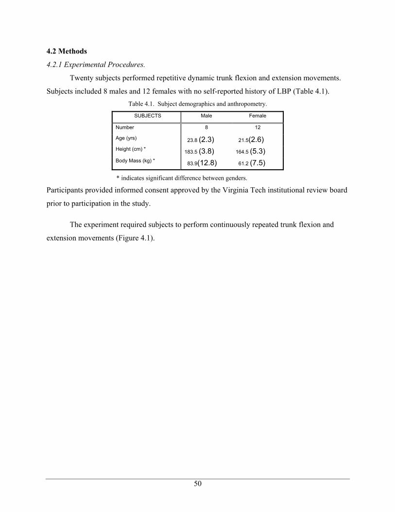
4.2 Methods

4.2.1 Experimental Procedures.

Twenty subjects performed repetitive dynamic trunk flexion and extension movements.

Subjects included 8 males and 12 females with no self-reported history of LBP (Table 4.1). Table 4.1. Subject demographics and anthropometry.

SUBJECTS Male Female

Number 8 12

Age (yrs) 23.8 (2.3) 21.5(2.6)

Height (cm) * 183.5 (3.8) 164.5 (5.3)

Body Mass (kg) * 83.9(12.8) 61.2 (7.5)

* indicates significant difference between genders.

Participants provided informed consent approved by the Virginia Tech institutional review board

prior to participation in the study.

The experiment required subjects to perform continuously repeated trunk flexion and

extension movements (Figure 4.1).

50

Figure 4.1. Experimental setup and schematic of the targeted movement task

They were required to touch targets with their hands held together. Targets were located at pre-

specified locations similar to methods described by Thomas 18. One target was placed at

shoulder height in the anterior sagittal midline so that the target could be reached when standing

upright with the arms horizontally extended. A second target was placed in the sagittal midline

50 cm anterior to the knee. Subjects were required to touch the upper target followed by the

lower target and continuously repeat this motion throughout the duration of each experimental

trial. Asymmetric trials were recorded wherein the upper target was moved to the right and the

lower target to the left so as to induce a nominal 450 axial rotation of the torso at the upper and

51

lower targets. Movements during these trials thereby included torso flexion and left twist.

Separate trials were conducted wherein the targets were placed so as to require flexion and right

twist. Each target was touched synchronous with a periodic tone from a metronome in order to

establish the movement pace, 20 and 40 cycles per minute. To assure 30 movement cycles per

trial the slow paced trials were 90 seconds in duration while the fast paced trials were 45 seconds

in duration. Although all movement cycles of each trial were recorded only the middle 15 cycles

were analyzed to assure steady-state movement behavior. Subjects were allowed to practice the

movements until they were comfortable with the movement trajectory and movement pace

before data collection of each trial. Experimental conditions were presented in randomized order

with at least two minutes rest between trials.

Upper-body kinematic data were recorded from electromagnetic motion sensors that were

secured by double-sided tape over the vertebral processes of the T10 and S1 (Ascension

Technology Corp., Burlington, VT). Trunk angles were computed by means of 3-D Euler

rotation matrices recorded from the T10 sensor with respect to the S1 sensor at a sample rate of

100 Hz. Following data collection, the kinematic data were filtered with a 10 Hz, low-pass, 2nd-

order Butterworth filter in preparation for calculation of dynamic stability. The number of data

samples per cycle can influence the estimate of stability 19. Therefore, the data were re-sampled

in software to obtain 4500 data samples per 15 movement cycles. Note that this provides a mean

value of 300 samples per cycle on average but cycle-to-cycle variability in movement duration

was retained. Expansion of kinematic variability in one dimension may be compensated by

contraction in another dimension. Thus, stability analyses were performed on the Euclidean

norm, i.e. square root of the sum of squares, of the three trunk angles recorded at each time

interval.

4.2.2 Calculating Dynamic Stability.

Local dynamic stability of the trunk flexion-extension movement was computed from the

maximum finite-time Lyapunov exponent, λMax. Complex dynamical systems must be

represented with greater number of dimensions than simple systems. However, the recorded data

were one-dimensional, time-series, column vectors, x(t), representing the Euclidean norm of the

trunk angles. One typical method of creating an n-dimensional state-space from scalar data is by

method of delays,

52

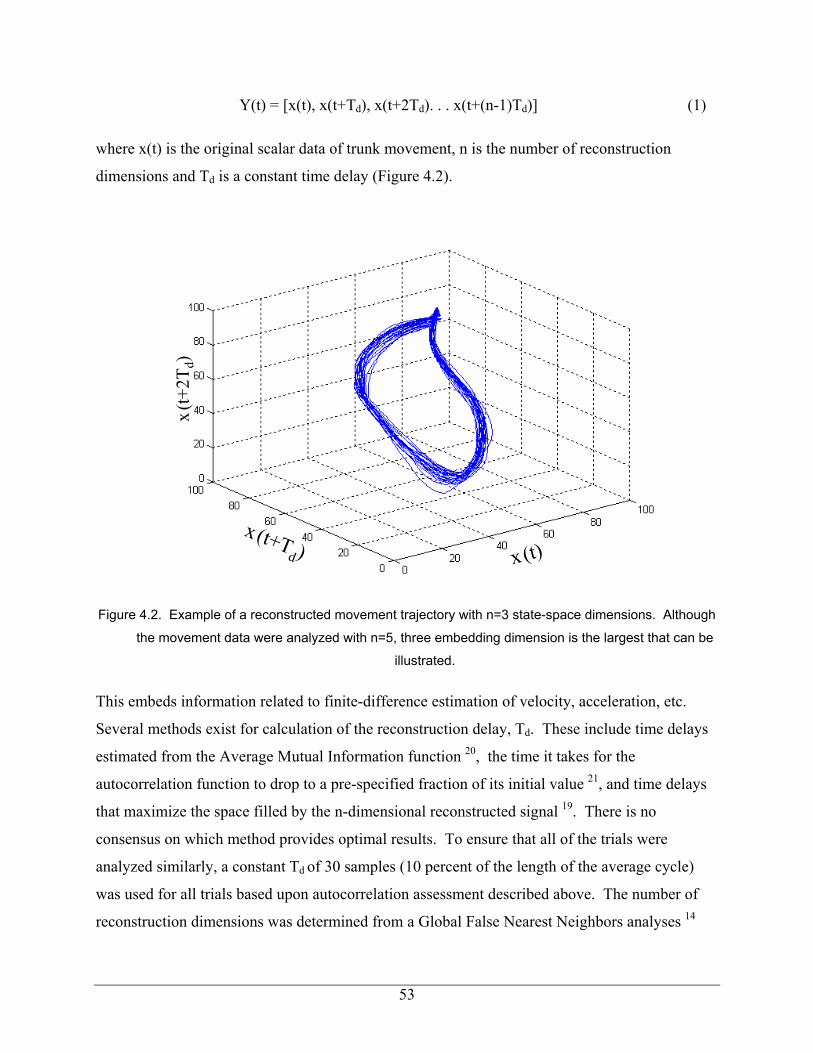
Y(t) = [x(t), x(t+Td), x(t+2Td). . . x(t+(n-1)Td)] (1)

where x(t) is the original scalar data of trunk movement, n is the number of reconstruction

dimensions and Td is a constant time delay (Figure 4.2).

x (t)x (t+T

d )

x(t+

2Td)

x (t)x (t+T

d )

x(t+

2Td)

Figure 4.2. Example of a reconstructed movement trajectory with n=3 state-space dimensions. Although

the movement data were analyzed with n=5, three embedding dimension is the largest that can be

illustrated.

This embeds information related to finite-difference estimation of velocity, acceleration, etc.

Several methods exist for calculation of the reconstruction delay, Td. These include time delays

estimated from the Average Mutual Information function 20, the time it takes for the

autocorrelation function to drop to a pre-specified fraction of its initial value 21, and time delays

that maximize the space filled by the n-dimensional reconstructed signal 19. There is no

consensus on which method provides optimal results. To ensure that all of the trials were

analyzed similarly, a constant Td of 30 samples (10 percent of the length of the average cycle)

was used for all trials based upon autocorrelation assessment described above. The number of

reconstruction dimensions was determined from a Global False Nearest Neighbors analyses 14

53

and revealed that an embedding dimension of n = 5 was appropriate for the analyzed data. False

nearest neighbors are defined as sets of points that are very close to each other at dimension n =

k but not at n = k+1. This method incrementally increases n until the number of false-nearest-

neighbors approaches zero.

Maximum finite-time Lyapunov exponents were calculated from the distance, di(t),

between nearest neighbors in the reconstructed state-space, Y(t). Nearest neighbors were found

by selecting data points from separate cycles that are closest to each other in the reconstructed

state-space (Figure 4.2). If repeated movement cycles were kinematically identical, then an

illustration of the trajectories would plot each cycle on top of the others. In this condition, the

distance between nearest neighbors, di(t), would be zero for all pairs of nearest neighbors, i.

However, in the empirically measured data the distance between nearest neighbors, di(t), was

greater than zero. Hence, there are clearly kinematic disturbances and/or chaotic behaviors

observable in the data. The distance between all nearest neighbors was tracked forward in time,

t. Since the growth in the least stable dimension quickly dominates expansion of the n-

dimensional sphere of kinematic variance, randomly selected initial trajectories should diverge,

on average, at a rate determined by the largest Lyapunov exponent, λMax 14. Therefore, the

maximum Lyapunov exponent, λMax was approximated as the slope of the linear best-fit line

created by the equation,

( ) ( )tdt

ty iln1∆

= (2)

where ( )tdiln represents the average logarithm of displacement, di(t), for all pairs of nearest

neighbors, i, throughout a time-span, t=0 to t=1 cycles (Figure 4.3).

54

0

0.5

1

1.5

2

2.5

0 0.5 1 1.5 2 2.5 3

Time (sec)

ln <

di(t

) >

λMAX

Figure 4.3 – Typical plot of the state-space expansion with time, ( ) ( )tdt

ty iln1∆

= . The dashed line

represents the best-fit line between t=0:1 cycles (with a cycle length of approximately 1.5 seconds for this

trial). The slope of the best-fit line was used to represent the state-space expansion, i.e. local dynamic

stability of the task

Stability is thereby calculated as λMax, which is the rate of divergence of initially neighboring

trajectories.

Statistical analyses were performed to determine the effect of movement pace and

asymmetry on the neuromuscular control of dynamic stability. Preliminary analyses revealed no

significant differences in λMax during asymmetric right-to-left versus left-to-right trials for the

number of subjects studies, (p=.437, F=0.617). Therefore, data from the two asymmetric

conditions were pooled for statistical analyses. Independent variables of movement pace (slow,

fast) and asymmetry (mid-sagittal, asymmetric) were treated as within-subject effects in a two-

factor repeated measures analysis of variance (ANOVA). Analyses were performed using

commercial software (Statsoft, Inc., Tulsa OK) using a significance level of α < 0.05.

55

4.3 Results

Maximum finite-time Lyapunov exponents, λMax, were calculated to estimate the

neuromuscular control of stability during repeated dynamic trunk flexion-extension movements

(Figure 4.4). A significant main effect for movement pace (p<0.001, F[1,19]=929.9) was

observed. Mean (standard deviation) values during repetitive trunk movement at 20 cycles per

minute were λMax = 0.397 (0.062) whereas when while moving at 40 cycles per minute λMax =

0.846 (0.098). Recall that larger values of λMax represent more rapidly diverging dynamics and

are considered less stable. Results suggest the value of the λMax during the fast trials were more

than twice the level recorded during slow dynamic movement. However, it would be incorrect to

infer from this that the slow movement was twice as stable unless the complete Lyapunov

spectrum were computed. Nonetheless, it can be concluded that the neuromuscular control of

dynamic stability declined significantly with increased movement rate.

A significant main effect for movement asymmetry was observed (p<.001, F[1,19]=28.5).

Sagittally symmetric movements were associated with greater λMax than asymmetric trials, 0.665

(0.256) and 0.579 (0.218) respectively. A pace-by-asymmetry interaction (p<0.018,

F[1,19]=6.69) revealed that the difference between slow and fast conditions was attenuated in the

asymmetric movement (Figure 4.4).

0

0.2

0.4

0.6

0.8

1

Slow FastMovement Pace

λMax

(mm

/sec

)

Symmetric Flexion

Asymmetric Flexion

Figure 4.4 – λMax values were greater during fast paced movement trials than slow paced cyclic

movement. Values were also greater during asymmetric movement tasks than during sagittal mid-plane

movements. Larger values of λMax represent less stable movement dynamics.

56

Nonetheless, the difference between slow and fast movements was statistically significant

(p<0.001) in both symmetric and asymmetric movement conditions.

57

4.4 Discussion

Musculoskeletal low-back injuries are often associated with dynamic trunk flexion 15.

Studies demonstrate that movement velocity influences torso muscle recruitment and co-

contraction thereby contributing to greater spinal load during fast paced lifting movements than

during slow movements 22. It is unclear why co-contraction might be increased during fast

movement. However, static 23;24 and quasi-static 25 analyses of lifting exertions suggest that co-

contraction may be recruited, in part, to augment spinal stability. Reduced spinal stability

combined with increased spinal compression may contribute to the risk associated with dynamic

trunk flexion. Although spinal stability has been estimated in static conditions 4, we are unaware

of any previous studies to quantify the neuromuscular control of stability during dynamic trunk

movements. Therefore the goal of this study was to determine whether the rate of movement

influences stability during dynamic trunk flexion and extension tasks

Neuromuscular control of stability declined with movement pace. Several factors may

contribute this behavior. First, momentum increases with movement velocity thereby requiring

greater neuromuscular effort to control and attenuate kinematic disturbances. Second, torso

muscle activity and co-contraction increase with trunk velocity and acceleration 26;27.

Modulation of muscle forces when muscle activity is high requires the recruitment of large motor

units thereby limiting fine-motor control during fast paced movements. Finally, fast dynamic

movements reduce the allowable time for neuromuscular corrections. This suggests increased

delay in the active recruitment and neural feedback relative to the movement trajectory.

Feedback delay is well recognized as a destabilizing factor in control systems 28. Fitt’s law of

motor control 29 suggests that greater kinematic errors may be expected when movement pace is

fast. Therefore, it is not surprising that neuro-control of dynamic stability was compromised

during the fast dynamic movement tasks.

Movements in the mid-sagittal plane were less stable than when moving in a combined

sagittal and twist trajectory. This contradicted our second hypothesis but may not be surprising

when one considers the neuromuscular control of these tasks. Published surface EMG

measurements suggest greater recruitment and coactivation of the internal and external oblique

muscle groups during asymmetric tasks 30;31. This recruitment is necessary to control the

asymmetric tasks whereas activation of these muscles is less critical when moving in the mid-

58

sagittal plane. Todorov 32 demonstrated that an optimal movement strategy may allow variability

in redundant, task-irrelevant dimensions, e.g. kinematic variability in the transverse plane during

mid-sagittal movement. When constraints were imposed by requiring simultaneous movement in

both the sagittal and transverse planes, increased control was required as documented by smaller

values of λMax. Further research is necessary to investigate how asymmetric trajectories

influence the control of dynamic movement. Specifically, the asymmetric movement in our

protocol resulted in movements that crossed the mid-sagittal plane, i.e. each movement included

rotation from left twist to right twist postures and vice versa. Moreover, the movement tasks did

not require handling of an external load. Representation of epidemiologic results should

investigate stability when the movement is confined to the left half-plane or right half-plane and

with a load in the hands. Nonetheless, results demonstrate that neuromuscular control patterns

associated with asymmetric movement trajectories significantly influences dynamic stability.

Understanding the meaning of the λMax coefficient is important when interpreting the

results. During static postural tasks the neuromuscular response to a kinematic perturbation will

cause the system to return toward the equilibrium state 10. Likewise, during dynamic torso

flexion and extension tasks the stabilizing neuromuscular control system will cause the

movement dynamics to be attracted toward the target movement trajectory. Recall that the

existence of an attractor trajectory represents a globally stable system is guaranteed when the

sum of the complete spectrum of Lyapunov exponents is negative, i.e. the rate of kinematic error

contraction is greater than the rate of expansion. Clearly, in our study the torso was stable for all

experimental conditions because there were no unbounded movements or injuries. Therefore, we

conclude that the sum of exponents was negative. However, the goal of the study was to

determine whether specific dynamic movement conditions were more or less stable than others.

The maximum Lyapunov exponent, λMax, characterizes the maximum time-rate of expansion for

the n-dimensional sphere that describes kinematic variability. In other words, this value

represents the least stable aspect of the movement dynamics 14. Consequently, it was logical to

investigate the maximum Lyapunov exponent, λMax, because it provides insight into the dynamic

behavior of the musculoskeletal system and it is mathematically feasible to estimate this

coefficient from empirical data. We hope to pursue further studies that will attempt to estimate

the full Lyapunov spectrum in order to provide greater insight into the neuromuscular control of

the spine. Moreover, future studies should investigate the nature of the maximum Lyapunov

59

exponent, λMax, in individual subjects. It represents local instability in a particular direction

thereby providing potential insight into the weakest control direction. It may be useful to

identify which kinematic dimensions are well controlled and which are poorly controlled in

individual patients for optimized prophylactic intervention or for design of individual-specific

injury rehabilitation.

An additional interesting result was the reconstruction dimension n=5. The

reconstruction dimension provides insight into the complexity of the neuromuscular dynamics.

Recall that the kinematics were represented as a one-dimensional Euclidean norm vector of the

trunk angles. Nonetheless, analyses revealed that the data must include at least 5 reconstructed

dimensions to adequately represent the dynamic system. We would not have been surprised with

n=3 when one recognizes that the trunk moved in 3-dimensions. A value of at least n=3 is

predicted by Taken’s theorem 33. However, the requirement of larger values, n=5, suggest that

multi-dimensional spinal curvature may have contributed to the results. This may indicate that

the analyses were sensitive to effects from spinal lordosis movement in addition to the global

trunk dynamics. Previous studies indicate that neuromuscular deficits in patients with low-back

pain are revealed most effectively in complex dynamical tasks 34. Whether the complexity of

neuromuscular control changes with movement task design and whether it is related to injury and

efficacy of rehabilitation should be investigated in future research.

In conclusion, nonlinear dynamical systems analyses were applied to empirically

recorded repetitive dynamic trunk movements. These analyses characterize the neuromuscular

control of stability during dynamic movements. Results demonstrate that both movement pace

and movement asymmetry influence the control of spinal stability. Continued development of

these stability assessment techniques are recommended for improved workplace design and

clinical assessment of spinal stability in patients with low-back pain.

4.5 Acknowledgements

This study was supported by grants R01 AR46111 from NIAMS of the National Institute

of Health and R01 OH07352-01 from NIOSH of the Centers of Disease Control.

60

References:

1. Panjabi M.M. The stabilizing system of the spine. Part I Function, dysfunction, adaptation

and enhancement. J.Spinal Disorders 1992;5:383-9.

2. Bergmark A. Stability of the lumbar spine: A study in mechanical engineering. Acta

Orthop.Scand.Suppl. 1989;230:1-54.

3. Gardner-Morse MG, Stokes IAF, and Laible JP. Role of muscles in lumbar stability in

maximum extension efforts. J.Orthop.Res. 1995;13:802-8.

4. Granata KP and Wilson SE. Trunk Posture and Spinal Stability. J.Biomechanics

2001;16:650-9.

5. Thompson J.M.T., Hunt G.W. The General Conservative Theory. Elastic Instability

Phenomena. New York: John Wiley & Sons, 1984:1-26.

6. Cholewicki J and McGill SM. Mechanical stability on the in vivo lumbar spine:

Implications for injury and chronic low back pain. Clin.Biomech. 1996;11:1-15.

7. Van Dieen JH, Cholewicki J, and Radebold A. Trunk muscle recruitment patterns in

patients with low back pain enhance the stability of the lumbar spine. Spine 2003;28:834-

41.

8. Cholewicki J, Polzhofer GA, and Radebold A. Postural control of trunk during unstable

sitting. J.Biomechanics 2000;22:1733-7.

9. Hodges PW, Gurfinkel VS, Brumagne S, Smith TC, and Cordo PC. Coexistence of stability

and mobility in postural control: evidence from postural compensation for respiration.

Exp.Brain Res. 2002;144:293-302.

10. Peterka RJ. Simplifying the complexities of maintaining balance. Ieee Engineering in

Medicine and Biology Magazine 2003;22:63-8.

61

11. Collins J.J. and DeLuca C.J. Open-loop and closed-loop control of posture: A random-walk

analysis of center of pressure. Exp.Brain Res. 1993;95:308-18.

12. Dingwell JB and Cusumano JP. Nonlinear time series analysis of normal and pathological

human walking. Chaos 2000;10:848-63.

13. Leipholz H. Stability Theory. An Introduction to the Stability of Dynamic Systems and

Rigid Bodies. New York: John Wiley & Sons, 1987.

14. Rosenstein MT, Collins JJ, and Deluca CJ. A Practical Method for Calculating Largest

Lyapunov Exponents from Small Data Sets. Physica D 1993;65:117-34.

15. National Research Council. Musculoskeletal Disorders and the Workplace. Washington

DC: National Academy Press, 2001.

16. Marras W.S., Lavender S.A., Leurgans S. et al. Biomechanical risk factors for

occupationally related low back disorder risk. Ergonomics 1995;38:377-410.

17. Fathallah F.A., Marras W.S., and Parnianpour M. The role of complex, simultaneous trunk

motions in the risk of occupation-related low back disorders. Spine 1998;23:1035-42.

18. Thomas JS, Corcos DM, and Hasan Z. Effect of movement speed on limb segment motions

for reaching from a standing position. Exp.Brain Res. 2003;148:377-87.

19. Rosenstein MT, Collins JJ, and Deluca CJ. Reconstruction Expansion As A Geometry-

Based Framework for Choosing Proper Delay Times. Physica D 1994;73:82-98.

20. Fraser AM and Swinney HL. Independent coordinates for strange attractors from mutual

information. Phys.Rev.A 1986;33:1134-40.

21. Albano AM, Muench J, Schwartz C, Mees AI, and Raap PE. Singular-value decomposition

and the Grassberger-Procaccia algorithm. Phys.Rev.A 1988;38:3017-26.

22. Granata KP and Marras WS. The influence of trunk muscle coactivity upon dynamic spinal

loads. Spine 1995;20:913-9.

62

23. Granata KP and Orishimo K. Response of Trunk Muscle Coactivation to Changes in Spinal

Stability. J.Biomechanics 2001;34:1117-23.

24. Gardner-Morse MG and Stokes IAF. The effects of abdominal muscle coactivation on

lumbar spine stability. Spine 1998;23:86-92.

25. Cholewicki J, Panjabi MM, and Khachatryan A. Stabilizing function of trunk flexor-

extensor muscles around a neutral spine posture. Spine 1997;22:2207-12.

26. Marras W.S. and Mirka GA. Electromyographic studies of the lumbar trunk musculature

during the generation of low-level trunk acceleration. Mirka G.A. 1993;11:811-7.

27. Dolan P. and Adams M.A. The relation between EMG activity and extensor moment

generation in the erector spinae muscles during bending and lifting activities.

J.Biomechanics, 1993;26:513-22.

28. Ogata K. Modern Control Engineering. 4 ed. Upper Saddle River, NJ: Prentice Hall, 2002.

29. Fitts P.M. The information capacity of the human motor system in controlling the

amplitude of movement. J.Exp.Psychol. 1954;47:381-91.

30. Lavender SA, Tsuang YH, Hafezi A, Andersson GB, Chaffin DB, and Hughes RE.

Coactivation of the trunk muscles during asymmetric loading of the torso. Hum.Factors

1992;34:239-47.

31. Granata KP and Marras WS. An EMG-assisted model of loads on the lumbar spine during

asymmetric trunk extensions. J.Biomechanics 1993;26:1429-38.

32. Todorov E and Jordan MI. Optimal feedback control as a theory of motor coordination.

Nature Neuroscience 2002;5:1226-35.

33. F.Takens. Detecting Strange Attractors in Turbulence. In: L.-S.Young, ed. Dynamical

Systems and Turbulence. New York: Springer, 1981:366-81.

63

34. Radebold A, Cholewicki J, Polzhofer GA, and Green TP. Impaired postural control of the

lumbar spine is associated with delayed muscle response times in patients with chronic

idiopathic low back pain. Spine 2001;26:724-30.

64

CONCLUSIONS

Local dynamic stability of the lower extremities during gait and the trunk during dynamic

flexion/extension motions were evaluated in this study. Results demonstrated that dynamic

stability is influenced by movement pace and symmetry, with reduced velocity and the presence

of asymmetry corresponding to more stable systems. Dynamic stability of several

musculoskeletal systems was successfully quantified in this study by means of maximum

Lyapunov exponent, λMax. Lyaponov exponents accurately measured the divergence of

kinematic trajectories describing the dynamics of the body during gait and trunk

flexion/extension motions. Lyapunov analysis provided insight into the roles various parameters

play in maintaining dynamic Lyapunov stability of the body. However, they leave the question

unanswered as to whether the body is neutrally or asymptotically stable while undergoing these

dynamic motions.

Neuromuscular control of stability was impaired by increased movement velocity. There

are several possible factors which may be responsible for this trend. Momentum of the analyzed

body segments increases with movement velocity thereby requiring greater neuromuscular effort

to control and reduce disturbances to the desired trajectory. Additionally, increased body

segment velocity can be linked to increased muscle activity and co-contraction in the associated

body segment. During periods of high muscle activity, control of muscle forces necessitates the

recruitment of large motor units thereby restricting fine-motor control during fast paced

movements. Fast movements also reduce the available time for neuromuscular corrections to

errors in the desired trajectory. This corresponds to increased delay in the active recruitment and

neural feedback relative to the movement trajectory. Feedback delay is widely accepted as a

destabilizing influence on control systems. Therefore, it is not surprising that neuro-control of

dynamic stability was deteriorated during the rapid movement tasks, however most previous

research on the influence of velocity on stability centered around kinematic variability as a

measure of stability.

Stability was also influenced by symmetry of motion of the trunk. It was observed that

asymmetric motions increased stability, contradicting our initial hypothesis. The may however

be attributable to increased muscle activity in asymmetric motion. Recruitment of more muscle

sets may assist in further constraining the motion and attenuating kinematic variability. Now

65

that controlling factors of musculoskeletal stability have been identified, further research is

appropriate to analyze the relationship between stability and injury. Identifying risk of injury

and possible solutions may lead to great gains in injury prevention as well as greater

understanding of neuromuscular control of the human body.

66

Appendix A – IRB approval

67

Appendix B – Subject Consent Form

Title of Project: Musculoskeletal Biomechanics of Movement and Control Investigators: S.A. England, K.P. Granata Purpose of this Research To understand musculoskeletal injury and improve clinical diagnoses of injury it is necessary to understand how muscles control force and movement. The purpose of this study is to measure the relation between human movement, force generation and muscle activity. We are also interested in observing how gender, fatigue and physical conditioning influence these parameters. Throughout the course of this project more than 200 subject volunteers will participate including healthy individuals from the age of 18 to 55. Procedures We will tape adhesive markers and sensors on your skin around your trunk, legs and arms. These sensors are EMG electrodes that measure the activity of your muscles and position sensors to measure how you move. After some preliminary warm up stretches, we may ask you to push and/or pull as hard as you can against a resistance. We may then ask you to hold or lift a weight or weighted-box and to bend forward and back. We may also ask you to do some fatiguing exertions such as holding or lifting a heavy weight or pushing/pulling against a bar or cable for several minutes. We may also apply a quick but small force to record reflexes. You may be requested to return for repeated testing. Between test sessions you may be asked to participate in specified physical conditioning as per the American College of Sports Medicine recommended guidelines Risks The risks of this study are minor. They include a potential skin irritation to the adhesives used in the tape and electrode markers. You may also feel some temporary muscle soreness such as might occur after exercising. Subjects participating in physical conditioning may experience muscle soreness and/or musculoskeletal injury associated with inherent risks of cardiovascular, strength training and therapeutic exercise. To minimize these risks you will be asked to warm-up before the tasks and tell us if you are aware of any history of skin-reaction to tape, history of musculoskeletal injury, cardiovascular limitations. Benefits By participating in this study, you will help to increase our understanding musculoskeletal control of movement and musculoskeletal injury mechanisms. We hope to make this research experience interesting and enjoyable for you where you may learn experimental procedures in biomechanical sciences. We do not guarantee or promise that you will receive any of these benefits and no promise of benefits has been made to encourage your participation. Anonymity and Confidentiality Experimental data collected from your participation will be coded and matched to this consent form so only members of the research team can determine your identity. Your identity will not be divulged to unauthorized people or agencies. Digital video recorded during the experimental trials will be used to track the movement of the sensors by means of computer analyses and is insufficient video quality to observe individual participant identifying characteristics. Secondary VHS-style video may be recorded to validate the digital motion data. This camera angle is placed to avoid facial or other identifying characteristics. Sometimes it is necessary for an investigator to break confidentiality if a significant health or safety concern is perceived or the participant is believed to be a threat to himself/herself or others. Compensation Participants required to return for multiple test sessions or participate in physical conditioning for this protocol will receive payment per the number of test sessions as well as a bonus for full completion of the multi-session research protocol. Subjects participating in experiments as part of course or laboratory procedures will receive appropriate credit for analysis of specified data as described in the course syllabus but not for personal performance during the experimental session. If course credit is involved and the

68

subject chooses not to participate alternative means for earning equivalent credit will be established with the course instructor. Freedom to Withdraw You are free to withdraw from a study at any time without penalty. If you choose to withdraw, you will be compensated for the portion of the time of the study (if financial compensation is involved). If you choose to withdraw, you will not be penalized by reduction in points or grade in a course (if course credit is involved). You are free not to answer any questions or respond to experimental situations that they choose without penalty. There may be circumstances under which the investigator may determine that you should not continue as a subject. You will be compensated for the portion of the project completed. Approval of Research This research project has been approved, as required, by the Institutional Review Board for Research Involving Human Subjects at Virginia Polytechnic Institute and State University, by the Department of Engineering science and Mechanics. 21 January 2003 20 January 2004 IRB Approval Date Approval Expiration Date

Subject's Responsibilities

I voluntarily agree to participate in this study. I have the following responsibilities: - Inform the investigators of all medical conditions that may influence performance or risk - Comply to the best of my ability with the experimental and safety instructions - Inform the investigator of any physical and mental discomfort resulting from the experimental

protocol Subject's Permission I have read and understand the Informed Consent and conditions of this project. I have had all my questions answered. I hereby acknowledge the above and give my voluntary consent: Subject Name (Print): Subject signature: Date Date Witness (Optional except for certain classes of subjects) Should I have any pertinent questions about this research or its conduct, and research subjects' rights, and whom to contact in the event of a research-related injury to the subject, I may contact: Investigator(s): Scott England E-mail: scenglan@vt.edu Phone 231-2022 Faculty Advisor: K.P. Granata E-mail: Granata@vt.edu Phone 231-7039 _______________________________________ ________________________ Departmental Reviewer/Department Head Telephone/e-mail

David M. Moore Chair, IRB Office of Research Compliance Research & Graduate Studies

Subjects must be given a complete copy (or duplicate original) of the signed Informed Consent

69

Appendix C – Lyapunov Analysis Flowchart

70

Appendix D – λMax data

λMax for ankles resampled to 3000 data points per 30 strides Subject # %Vf 20 40 60 80

205 0.7272183 1.0138974 1.1786728 1.7539433207 0.6194175 0.7526825 1.0053446 1.5097501209 0.599869 0.904352 1.0498849 1.7879275210 0.6607085 0.9259156 1.2544687 1.818659211 0.682159 0.9725583 1.1551931 1.7251992213 0.7336615 0.8810039 1.1471708 1.7065829214 0.6443746 0.8052548 1.1310564 1.5533956215 0.7894467 0.9497256 1.0816004 1.5535721216 0.7639953 0.9692452 1.2022564 1.5814725217 0.8368418 0.6179801 1.0449138 1.4478857218 0.7002333 0.8132258 0.9991141 1.5564771219 0.8580868 0.9393106 0.995016 1.3935454220 0.5948015 0.7656096 1.1680128 1.7191033221 0.686555 0.917076 1.1863157 1.8304287222 0.5820105 0.89601 1.1221981 1.5225625223 0.771598 0.9309176 1.1736197 1.5523031226 0.741326 0.9263708 0.9407499 1.3489811227 0.6664139 0.9096483 1.1721028 1.6064042228 0.8141734 1.0365659 1.2528386 1.5803072230 0.7825194 0.8835441 1.062318 1.6537451

71

λMax for knees resampled to 3000 data points per 30 strides Subject # %Vf 20 40 60 80

205 0.9651904 1.2783802 1.4501147 1.8881418207 0.78979 0.9620883 1.3599951 1.7252096209 0.8717667 1.3382975 1.462948 2.0865829210 0.8785253 1.1052421 1.6173815 2.2693948211 0.889055 1.4124682 1.6801606 1.957183213 1.0058941 1.3806194 1.5654837 1.987908214 0.8900763 1.3631159 1.5782188 1.7333028215 1.1411236 1.3393685 1.4472828 1.8773767216 1.021053 1.3512778 1.5956023 2.0787755217 1.1918704 1.2087436 1.4396625 2.0003602218 0.8024942 0.9756334 1.2938068 1.8373584219 1.2584254 1.4060288 1.466235 1.787581220 0.8690033 1.1625216 1.4854137 1.9998255221 0.969137 1.3519517 1.5918245 1.992432222 0.7669467 1.178156 1.4661155 1.7956166223 1.1598148 1.2599851 1.5955009 1.7941447226 0.9081709 1.2904294 1.3422061 1.6040248227 0.8264286 1.2557386 1.5474214 1.7385146228 1.0416086 1.2603774 1.6178144 1.7367113230 1.0041196 1.2888003 1.5153168 1.9671134

72

λMax for hips resampled to 3000 data points per 30 strides Subject # %Vf 20 40 60 80

205 0.8942184 1.1722291 1.5068881 1.8126258207 0.7626155 1.0650085 1.2365581 1.6076463209 0.8526064 1.1599922 1.2713452 1.8965133210 0.8535659 1.0101229 1.4148689 2.0739299211 0.7838367 1.2055431 1.2903145 1.7591777213 0.9078785 1.1568494 1.4689672 1.9414758214 0.8295539 1.1953499 1.342654 1.5985992215 0.9988124 1.0318077 1.1948822 1.6530321216 0.9554976 1.2080241 1.3877934 1.7708222217 1.0019511 1.0078785 1.1791474 1.5314347218 0.710377 1.0012662 1.1701982 1.5821891219 0.8971009 1.0669167 1.2155769 1.539061220 0.7586089 0.985901 1.2649605 1.7470436221 0.8700415 1.2241099 1.4400262 1.8566561222 0.7513254 1.046303 1.3867024 1.7145873223 1.0673593 0.996227 1.3698668 1.5912867226 0.8575313 1.0981833 1.1032222 1.4504377227 0.770337 1.127669 1.3529747 1.7924709228 1.0141993 1.1172814 1.3362281 1.6549216230 0.9384074 1.1178607 1.2155163 1.9723528

73

λMax for ankles resampled to 100 data points per stride Subject # %Vf 20 40 60 80

205 0.441268 0.868685 1.286087 1.5772286207 0.517633 0.650025 0.789835 1.4687265209 0.37648 0.802083 0.935563 1.5787204210 0.440533 0.79281 0.929057 1.4187245211 0.361963 0.642549 0.869402 1.4563632213 0.411888 0.716682 1.000886 1.4142037214 0.424966 0.660418 0.910784 1.2974267215 0.47909 0.961083 0.980472 1.4705333216 0.37137 0.744987 0.935163 1.321089217 0.571159 0.624844 0.816812 1.3189111219 0.618195 0.778896 0.965 1.2603224220 0.361866 0.596397 0.915918 1.4113743221 0.565602 0.796329 1.106256 1.6516474222 0.50012 0.770259 0.900941 1.3214158223 0.529535 0.673029 0.897483 1.2255145226 0.279199 0.606199 0.883472 1.1547386227 0.465686 0.688489 0.95141 1.2936087228 0.447136 0.789906 1.118557 1.5166509230 0.675844 0.572584 0.770501 1.4142864

74

λMax for knees resampled to 100 data points per stride Subject # %Vf 20 40 60 80

205 0.580017 0.976207 1.275308 1.6124859207 0.580401 0.869369 1.238341 1.6478659209 0.481718 0.982194 1.171419 1.7862783210 0.700607 1.042624 1.299356 1.6374883211 0.429824 0.977794 1.269316 1.7737152213 0.589105 1.055047 1.247406 1.6695475214 0.469116 0.956624 1.263116 1.464137215 0.759443 1.261862 1.236345 1.8795827216 0.769286 1.08287 1.400548 1.6516032217 0.666498 0.978483 1.209575 1.7055222219 1.033769 1.007655 1.330005 1.6768347220 0.70253 0.988711 1.295652 1.6890282221 0.897103 1.1675 1.317126 1.8363906222 0.581433 1.029663 1.215386 1.5631541223 0.923885 0.995438 1.333548 1.5267543226 0.381167 0.729183 1.1746 1.3801386227 0.860983 1.096793 1.251255 1.5215983228 0.896408 1.115314 1.461113 1.574671230 0.961892 1.013949 1.35776 1.7640122

75

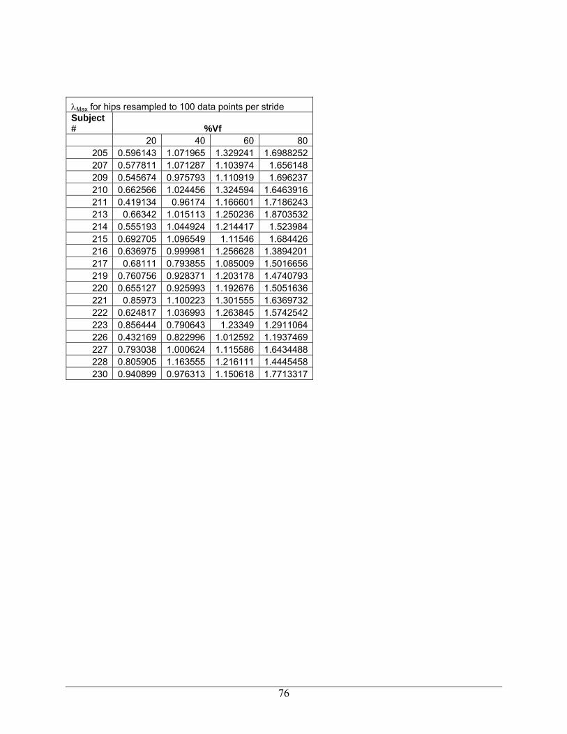
λMax for hips resampled to 100 data points per stride Subject # %Vf 20 40 60 80

205 0.596143 1.071965 1.329241 1.6988252207 0.577811 1.071287 1.103974 1.656148209 0.545674 0.975793 1.110919 1.696237210 0.662566 1.024456 1.324594 1.6463916211 0.419134 0.96174 1.166601 1.7186243213 0.66342 1.015113 1.250236 1.8703532214 0.555193 1.044924 1.214417 1.523984215 0.692705 1.096549 1.11546 1.684426216 0.636975 0.999981 1.256628 1.3894201217 0.68111 0.793855 1.085009 1.5016656219 0.760756 0.928371 1.203178 1.4740793220 0.655127 0.925993 1.192676 1.5051636221 0.85973 1.100223 1.301555 1.6369732222 0.624817 1.036993 1.263845 1.5742542223 0.856444 0.790643 1.23349 1.2911064226 0.432169 0.822996 1.012592 1.1937469227 0.793038 1.000624 1.115586 1.6434488228 0.805905 1.163555 1.216111 1.4445458230 0.940899 0.976313 1.150618 1.7713317

76

λmax for trunk flexion angle SLOW FAST Subject # V DR DL V DR DL G

101 0.634769 0.455467 0.355948 0.949935 0.667897 0.728056 1 102 0.559131 0.332169 0.413618 1.012453 0.815209 0.721242 1 103 0.563844 0.387742 0.449469 0.903053 0.669139 0.7718 1 104 0.604321 0.361682 0.422168 0.82885 0.840707 0.739775 1 105 0.571801 0.371755 0.439271 0.978776 0.78189 0.663175 1 106 0.42904 0.462139 0.28832 0.858312 0.874012 0.976 1 107 0.491747 0.395077 0.354168 1.052074 0.893084 0.834135 1 108 0.502496 0.429295 0.341929 0.967844 0.70782 0.642557 1 109 0.433659 0.291713 0.426838 0.884749 0.778385 0.752542 1 110 0.455413 0.343093 0.356434 0.924542 0.696862 0.732354 1 111 0.534156 0.333778 0.296707 0.791203 0.752724 0.808433 1 112 0.451056 0.362905 0.338716 0.85942 0.924377 0.867368 1 113 0.49696 0.355293 0.306616 0.853782 0.692324 0.739154 1 114 0.652961 0.302354 0.344217 0.990628 0.770659 0.899874 1 115 0.673943 0.316117 0.435853 1.002482 0.62683 0.711876 1 116 0.532605 0.261005 0.352162 0.831225 0.623124 0.636042 2 117 0.646785 0.318587 0.337597 0.863016 0.729925 0.806873 2 118 0.523004 0.319069 0.455261 0.950279 0.701616 0.759431 2 119 0.504322 0.404718 0.223411 0.738197 0.782313 0.659393 2 120 0.502872 0.288318 0.425565 0.892524 0.827339 0.694583 2 121 0.523556 0.530657 0.403498 0.977944 0.590104 0.647077 2 122 0.534712 0.407567 0.352236 0.849062 0.753412 0.815336 2 123 0.308113 0.374444 0.419726 1.063033 0.961813 0.89311 2 124 0.500964 0.268695 0.350185 0.912011 0.686287 0.933017 2 125 0.429145 0.396075 0.327581 1.013741 0.765767 0.756577 2 126 0.610944 0.504043 0.422507 0.962616 0.786439 0.761792 2 127 0.540335 0.48013 0.304705 0.911741 0.827648 0.813543 2 128 0.500979 0.37757 0.368074 0.951365 0.913333 0.644809 2 129 0.557348 0.349087 0.485971 0.972997 0.691989 0.770087 2 130 0.474669 0.460363 0.375646 1.044016 0.832351 0.830836 2

77

Appendix E – Gait Analysis Matlab Program

clear all close all numberofstrides=15; datapointsperstride=100; tic subjectnumberint=230; vf=80; nametosave=[int2str(subjectnumberint) 'vf' int2str(vf)] name=nametosave; subjectnumber=[int2str(subjectnumberint) '_' int2str(vf) 'vf'] row=subjectnumberint-200+1; column=vf/20+1; filename=['C:\MATLAB6p1\work\gait data mat files\' subjectnumber '.mat']; load(filename) fs = 100; % Sampling Frequency in hertz fn = fs/2; % Nyquist Frequency fc = 10; % Cut-off frequency for 2nd order butterworth filter [b,a] = butter(2, fc/fn); data = filtfilt(b,a,markerposition); %data = markerposition; % Assign names to each trajectory sacr(:,1:3) = data(:,1,1:3); lasi(:,1:3) = data(:,2,1:3); rasi(:,1:3) = data(:,3,1:3); lpsi(:,1:3) = data(:,4,1:3); rpsi(:,1:3) = data(:,5,1:3); lthi(:,1:3) = data(:,6,1:3); lkne(:,1:3) = data(:,7,1:3); ltib(:,1:3) = data(:,8,1:3); lank(:,1:3) = data(:,9,1:3); lhee(:,1:3) = data(:,10,1:3); lmt5(:,1:3) = data(:,11,1:3); ldor(:,1:3) = data(:,12,1:3); ltoe(:,1:3) = data(:,13,1:3); rthi(:,1:3) = data(:,14,1:3); rkne(:,1:3) = data(:,15,1:3); rtib(:,1:3) = data(:,16,1:3); rank(:,1:3) = data(:,17,1:3); rhee(:,1:3) = data(:,18,1:3); rmt5(:,1:3) = data(:,19,1:3); rdor(:,1:3) = data(:,20,1:3); rtoe(:,1:3) = data(:,21,1:3); %hip joint centers parameters beta=18.0*pi/180;%degrees

78

theta=28.4*pi/180;%degrees mm=0.0145;%marker radius t=length(data); for i =1:t %HIP CENTER STUFF dASIS=sqrt((lasi(i,1)-rasi(i,1))^2+(lasi(i,2)-rasi(i,2))^2+(lasi(i,3)-rasi(i,3))^2); lengthrightleg=sqrt((rasi(i,1)-rkne(i,1))^2+(rasi(i,2)-rkne(i,2))^2+(rasi(i,3)-rkne(i,3))^2)+sqrt((rkne(i,1)-rank(i,1))^2+(rkne(i,2)-rank(i,2))^2+(rkne(i,3)-rank(i,3))^2); lengthleftleg=sqrt((lkne(i,1)-lank(i,1))^2+(lkne(i,2)-lank(i,2))^2+(lkne(i,3)-lank(i,3))^2)+sqrt((lasi(i,1)-lkne(i,1))^2+(lasi(i,2)-lkne(i,2))^2+(lasi(i,3)-lkne(i,3))^2); leglength=(lengthrightleg+lengthleftleg)/2; C=leglength*0.115-0.0153; LATD=0.1288*leglength-0.04856; RATD=LATD; aa=dASIS/2; PELF=(rasi(i,1:3)+lasi(i,1:3))/2; pelf(i,1:3)=PELF; LHJCz=(-C*cos(theta)*cos(beta)-(LATD+mm)*sin(beta)); RHJCz=(-C*cos(theta)*cos(beta)-(RATD+mm)*sin(beta)); LHJCy=(C*cos(theta)*sin(beta)-(LATD+mm)*cos(beta)); RHJCy=(C*cos(theta)*sin(beta)-(RATD+mm)*cos(beta)); LHJCx=(-C*sin(theta)+aa); RHJCx=(C*sin(theta)-aa); %finding rotation to move HJCs %alpha=atan2(lasi(i,3)-rasi(i,3),lasi(i,2)-rasi(i,2)); alpha=atan2(sacr(i,3)-pelf(i,3),sacr(i,2)-pelf(i,2)); gamma=atan2(lasi(i,3)-rasi(i,3),lasi(i,1)-rasi(i,1)); delta=atan2(lasi(i,2)-rasi(i,2),lasi(i,1)-rasi(i,1)); angles(i,:)=[alpha,gamma,delta]; Rx=[1,0,0;0,cos(alpha),sin(alpha);0,-sin(alpha),cos(alpha)]; Ry=[cos(gamma),0,-sin(gamma);0,1,0;sin(gamma),0,cos(gamma)]; Rz=[cos(delta),sin(delta),0;-sin(delta),cos(delta),0;0,0,1]; R=Rx*Ry*Rz; LHJCr=R*[LHJCx;LHJCy;LHJCz]; RHJCr=R*[RHJCx;RHJCy;RHJCz]; LHJC=[PELF(1)+LHJCr(1),PELF(2)-LHJCr(2),PELF(3)+LHJCr(3)]; RHJC=[PELF(1)+RHJCr(1),PELF(2)-RHJCr(2),PELF(3)+RHJCr(3)]; RHJCtotal(i,:)=RHJC; LHJCtotal(i,:)=LHJC;

79

%Define limb vectors to use in determining angle between them rightshin=[(rkne(i,1)-rank(i,1)),(rkne(i,2)-rank(i,2)),(rkne(i,3)-rank(i,3))]; magrightshin=sqrt((rkne(i,1)-rank(i,1))^2+(rkne(i,2)-rank(i,2))^2+(rkne(i,3)-rank(i,3))^2); rightfoot=[(rmt5(i,1)-rank(i,1)),(rmt5(i,2)-rank(i,2)),(rmt5(i,3)-rank(i,3))]; magrightfoot=sqrt((rmt5(i,1)-rank(i,1))^2+(rmt5(i,2)-rank(i,2))^2+(rmt5(i,3)-rank(i,3))^2); leftshin=[(lkne(i,1)-lank(i,1)),(lkne(i,2)-lank(i,2)),(lkne(i,3)-lank(i,3))]; magleftshin=sqrt((lkne(i,1)-lank(i,1))^2+(lkne(i,2)-lank(i,2))^2+(lkne(i,3)-lank(i,3))^2); leftfoot=[(lmt5(i,1)-lank(i,1)),(lmt5(i,2)-lank(i,2)),(lmt5(i,3)-lank(i,3))]; magleftfoot=sqrt((lmt5(i,1)-lank(i,1))^2+(lmt5(i,2)-lank(i,2))^2+(lmt5(i,3)-lank(i,3))^2); rightthigh=[(RHJC(1)-rkne(i,1)),(RHJC(2)-rkne(i,2)),(RHJC(3)-rkne(i,3))]; magrightthigh=sqrt((RHJC(1)-rkne(i,1))^2+(RHJC(2)-rkne(i,2))^2+(RHJC(3)-rkne(i,3))^2); righthip=[(rpsi(i,1)-rasi(i,1)),(rpsi(i,2)-rasi(i,2)),(rpsi(i,3)-rasi(i,3))]; magrighthip=sqrt((rpsi(i,1)-rasi(i,1))^2+(rpsi(i,2)-rasi(i,2))^2+(rpsi(i,3)-rasi(i,3))^2); leftthigh=[(LHJC(1)-lkne(i,1)),(LHJC(2)-lkne(i,2)),(LHJC(3)-lkne(i,3))]; magleftthigh=sqrt((LHJC(1)-lkne(i,1))^2+(LHJC(2)-lkne(i,2))^2+(LHJC(3)-lkne(i,3))^2); lefthip=[(lpsi(i,1)-lasi(i,1)),(lpsi(i,2)-lasi(i,2)),(lpsi(i,3)-lasi(i,3))]; maglefthip=sqrt((lpsi(i,1)-lasi(i,1))^2+(lpsi(i,2)-lasi(i,2))^2+(lpsi(i,3)-lasi(i,3))^2); RA(i)=(acos(dot(rightshin,rightfoot)/(magrightshin*magrightfoot))*180/pi); LA(i)=(acos(dot(leftshin,leftfoot)/(magleftshin*magleftfoot))*180/pi); RK(i)=(acos(dot(rightshin,rightthigh)/(magrightshin*magrightthigh))*180/pi); LK(i)=(acos(dot(leftshin,leftthigh)/(magleftshin*magleftthigh))*180/pi); RH(i)=(acos(dot(righthip,rightthigh)/(magrighthip*magrightthigh))*180/pi); LH(i)=(acos(dot(lefthip,leftthigh)/(maglefthip*magleftthigh))*180/pi); end RA=transpose(RA); LA=transpose(LA); RK=transpose(RK); LK=transpose(LK); RH=transpose(RH); LH=transpose(LH); i=1:t; figure(1) subplot(2,1,1) plot(i,RH) title('Right Hip Angle vs time') xlabel('Time') ylabel('Angle') subplot(2,1,2)

80

plot(i,LH) title('Left Hip Angle vs time') xlabel('Time') ylabel('Angle') figure(2) subplot(2,1,1) plot(i,RK) title('Right Knee Angle vs time') xlabel('Time') ylabel('Angle of Flexion') subplot(2,1,2) plot(i,LK) title('Left Knee Angle vs time') xlabel('Time') ylabel('Angle of Flexion') figure(3) subplot(2,1,1) plot(i,RA) title('Right Ankle Angle vs time') xlabel('Time') ylabel('Angle of Plantar Flexion') subplot(2,1,2) plot(i,LA) title('Left Ankle Angle vs time') xlabel('Time') ylabel('Angle of Plantar Flexion') %%%Here's the stuff for variability measures TOH=input('Counting toe off (1) or heel off (2) or crash it(3): '); if TOH==3 crashitnowthedatasucks else end % %start pulling out peaks and splining in between them if desired % for n=1:numberofstrides+1 % [X,Y]=ginput(2); % if TOH==1 % [uselesspeak,I]=max(RA(round(X(1)):round(X(2)))); % else % [uselesspeak,I]=min(RA(round(X(1)):round(X(2)))); % end % hold on % subplot(2,1,1) % plot(I+round(X(1))-1,uselesspeak,'rX') % timeofpeaksRs(n+1)=[I+round(X(1))-1]; % uselesspeaksR(n)=uselesspeak; % end % %now spline % for p=1:numberofstrides % xRs=timeofpeaksRs(p+1):timeofpeaksRs(p+2); % xxRs=linspace(timeofpeaksRs(p+1),timeofpeaksRs(p+2),101);

81

% rangeofRAs=RA(timeofpeaksRs(p+1):timeofpeaksRs(p+2)); % rangeofRKs=RK(timeofpeaksRs(p+1):timeofpeaksRs(p+2)); % rangeofRHs=RH(timeofpeaksRs(p+1):timeofpeaksRs(p+2)); % splinedRAs=spline(xRs,rangeofRAs,xxRs); % splinedRKs=spline(xRs,rangeofRKs,xxRs); % splinedRHs=spline(xRs,rangeofRHs,xxRs); % rightankleangles(p,:)=splinedRAs; % rightkneeangles(p,:)=splinedRKs; % righthipangles(p,:)=splinedRHs; % end % stringofRAs=rightankleangles(1,1:100); %this just sets the beginning so i can add onto stringofangles % stringofRKs=rightkneeangles(1,1:100); % stringofRHs=righthipangles(1,1:100); % % for q=2:numberofstrides % stringofRAs=[stringofRAs,rightankleangles(q,1:100)]; % stringofRKs=[stringofRKs,rightkneeangles(q,1:100)]; % stringofRHs=[stringofRHs,righthipangles(q,1:100)]; % end % input('press enter to continue now with the left ankle'); % for n=1:numberofstrides+1 % [X,Y]=ginput(2); % if TOH==1 % [uselesspeak,I]=max(LA(round(X(1)):round(X(2)))); % else % [uselesspeak,I]=min(LA(round(X(1)):round(X(2)))); % end % hold on % subplot(2,1,2) % plot(I+round(X(1))-1,uselesspeak,'rX') % timeofpeaksLs(n+1)=[I+round(X(1))-1]; % uselesspeaksL(n)=uselesspeak; % end % %now spline % for p=1:numberofstrides % xLs=timeofpeaksLs(p+1):timeofpeaksLs(p+2); % xxLs=linspace(timeofpeaksLs(p+1),timeofpeaksLs(p+2),101); % rangeofLAs=LA(timeofpeaksLs(p+1):timeofpeaksLs(p+2)); % rangeofLKs=LK(timeofpeaksLs(p+1):timeofpeaksLs(p+2)); % rangeofLHs=LH(timeofpeaksLs(p+1):timeofpeaksLs(p+2)); % splinedLAs=spline(xLs,rangeofLAs,xxLs); % splinedLKs=spline(xLs,rangeofLKs,xxLs); % splinedLHs=spline(xLs,rangeofLHs,xxLs); % leftankleangles(p,:)=splinedLAs; % leftkneeangles(p,:)=splinedLKs; % lefthipangles(p,:)=splinedLHs; % end % stringofLAs=leftankleangles(1,1:100); %this just sets the beginning so i can add onto stringofangles % stringofLKs=leftkneeangles(1,1:100); % stringofLHs=lefthipangles(1,1:100); % % % % for q=2:numberofstrides % stringofLAs=[stringofLAs,leftankleangles(q,1:100)]; % stringofLKs=[stringofLKs,leftkneeangles(q,1:100)];

82

% stringofLHs=[stringofLHs,lefthipangles(q,1:100)]; % end % % for n=1:numberofstrides % averagetime(n)=timeofpeaksRs(n+2)-timeofpeaksRs(n+1); % end % %format short % averagestridetime=sum(averagetime)/(numberofstrides) % peakRs=mean(uselesspeaksR); % peakLs=mean(uselesspeaksL); % hold on % for n=1:numberofstrides+1 % subplot(2,1,1) % plot(timeofpeaksRs(2)+averagestridetime*(n-1),peakRs,'rX') % subplot(2,1,2) % plot(timeofpeaksLs(2)+averagestridetime*(n-1),peakLs,'rX') % end % % %%% save RA_subjectnumber % % newfilenameRAs=['ras' nametosave '.txt']; % newfilenameLAs=['las' nametosave '.txt']; % newfilenameRKs=['rks' nametosave '.txt']; % newfilenameLKs=['lks' nametosave '.txt']; % newfilenameRHs=['rhs' nametosave '.txt']; % newfilenameLHs=['lhs' nametosave '.txt']; % % %first make a giant matrix of values 30 rows, 100 columns for each measure % for n=1:30 % for o=1:100 % STDEVA_MATRIX_RA(n,o)=stringofRAs((n-1)*100+o); % STDEVA_MATRIX_LA(n,o)=stringofLAs((n-1)*100+o); % % STDEVA_MATRIX_RK(n,o)=stringofRKs((n-1)*100+o); % STDEVA_MATRIX_LK(n,o)=stringofLKs((n-1)*100+o); % % STDEVA_MATRIX_RH(n,o)=stringofRHs((n-1)*100+o); % STDEVA_MATRIX_LH(n,o)=stringofLHs((n-1)*100+o); % end % end % % STD_VECTOR_RA=std(STDEVA_MATRIX_RA); % STD_VECTOR_LA=std(STDEVA_MATRIX_LA); % % STD_VECTOR_RK=std(STDEVA_MATRIX_RK); % STD_VECTOR_LK=std(STDEVA_MATRIX_LK); % % STD_VECTOR_RH=std(STDEVA_MATRIX_RH); % STD_VECTOR_LH=std(STDEVA_MATRIX_LH); % % STD_TRIAL_RA=mean(STD_VECTOR_RA); % STD_TRIAL_LA=mean(STD_VECTOR_LA); % % STD_TRIAL_RK=mean(STD_VECTOR_RK); % STD_TRIAL_LK=mean(STD_VECTOR_LK); %

83

% STD_TRIAL_RH=mean(STD_VECTOR_RH); % STD_TRIAL_LH=mean(STD_VECTOR_LH); % % RASTDEVA=dlmread('RASTDEVA.txt','\t',[0,0,30,4]); % LASTDEVA=dlmread('LASTDEVA.txt','\t',[0,0,30,4]); % % RKSTDEVA=dlmread('RKSTDEVA.txt','\t',[0,0,30,4]); % LKSTDEVA=dlmread('LKSTDEVA.txt','\t',[0,0,30,4]); % % RHSTDEVA=dlmread('RHSTDEVA.txt','\t',[0,0,30,4]); % LHSTDEVA=dlmread('LHSTDEVA.txt','\t',[0,0,30,4]); % % RASTDEVA(row,column)=STD_TRIAL_RA; % LASTDEVA(row,column)=STD_TRIAL_LA; % % RKSTDEVA(row,column)=STD_TRIAL_RK; % LKSTDEVA(row,column)=STD_TRIAL_LK; % % RHSTDEVA(row,column)=STD_TRIAL_RH; % LHSTDEVA(row,column)=STD_TRIAL_LH; % % save RASTDEVA.txt RASTDEVA -ascii -double -tabs % save LASTDEVA.txt LASTDEVA -ascii -double -tabs % % save RKSTDEVA.txt RKSTDEVA -ascii -double -tabs % save LKSTDEVA.txt LKSTDEVA -ascii -double -tabs % % save RHSTDEVA.txt RHSTDEVA -ascii -double -tabs % save LHSTDEVA.txt LHSTDEVA -ascii -double -tabs % % save(newfilenameRAs,'stringofRAs','-ascii','-tabs','-double') % save(newfilenameLAs,'stringofLAs','-ascii','-tabs','-double') % save(newfilenameRKs,'stringofRKs','-ascii','-tabs','-double') % save(newfilenameLKs,'stringofLKs','-ascii','-tabs','-double') % save(newfilenameRHs,'stringofRHs','-ascii','-tabs','-double') % save(newfilenameLHs,'stringofLHs','-ascii','-tabs','-double') % % % clear stringofRAs stringofLAs stringofRKs stringofLKs stringofRHs stringofLHs averagestridetime=input('average stride time from excel spreadsheet: '); %%% and now back to the old stuff % uncomment this when going back to dynamic stability and variability % figure(10) % subplot(2,1,1) % plot(i,RA) % title('Right Ankle Angle vs time') % xlabel('Time') % ylabel('Angle of Plantar Flexion') % subplot(2,1,2) % plot(i,LA)

84

% title('Left Ankle Angle vs time') % xlabel('Time') % ylabel('Angle of Plantar Flexion') %grab the first and last peak and splines 3000 points between them for n=1:2 [X,Y]=ginput(2); if TOH==1 [uselesspeak,I]=max(RA(round(X(1)):round(X(2)))); else [uselesspeak,I]=min(RA(round(X(1)):round(X(2)))); end hold on if n==1 subplot(2,1,1) plot(I+round(X(1))-1,uselesspeak,'rX') timeofpeaksR(n+1)=[I+round(X(1))-1]; uselesspeaksR(n)=uselesspeak; for j=1:numberofstrides-1 plot(timeofpeaksR(n+1)+averagestridetime*j,uselesspeaksR(1),'rX') end elseif n==2 subplot(2,1,1) plot(I+round(X(1))-1,uselesspeak,'bO') timeofpeaksR(n+1)=[I+round(X(1))-1]; uselesspeaksR(n)=uselesspeak; end end %now count them out % rightankleangle(1,:)=RA(timeofpeaksR(2):timeofpeaksR(3)); % rightkneeangle(1,:)=RK(timeofpeaksR(2):timeofpeaksR(3)); % righthipangle(1,:)=RH(timeofpeaksR(2):timeofpeaksR(3)); xR=timeofpeaksR(2):timeofpeaksR(3); xxR=linspace(timeofpeaksR(2),timeofpeaksR(3),numberofstrides*datapointsperstride);%This will now 30 full strides into 3000 data points rangeofRA=RA(timeofpeaksR(2):timeofpeaksR(3)); %change both right and left numbers rangeofRK=RK(timeofpeaksR(2):timeofpeaksR(3)); rangeofRH=RH(timeofpeaksR(2):timeofpeaksR(3)); splinedRA=spline(xR,rangeofRA,xxR); splinedRK=spline(xR,rangeofRK,xxR); splinedRH=spline(xR,rangeofRH,xxR); rightankleangle(1,:)=splinedRA; rightkneeangle(1,:)=splinedRK; righthipangle(1,:)=splinedRH; stringofRA=rightankleangle; stringofRK=rightkneeangle; stringofRH=righthipangle;

85

input('press enter to continue now with the left ankle'); for n=1:2 [X,Y]=ginput(2); if TOH==1 [uselesspeak,I]=max(LA(round(X(1)):round(X(2)))); else [uselesspeak,I]=min(LA(round(X(1)):round(X(2)))); end hold on if n==1 subplot(2,1,2) plot(I+round(X(1))-1,uselesspeak,'rX') timeofpeaksL(n+1)=[I+round(X(1))-1]; uselesspeaksL(n)=uselesspeak; for j=1:numberofstrides-1 plot(timeofpeaksL(n+1)+averagestridetime*j,uselesspeaksL(1),'rX') end elseif n==2 subplot(2,1,2) plot(I+round(X(1))-1,uselesspeak,'bO') timeofpeaksL(n+1)=[I+round(X(1))-1]; uselesspeaksL(n)=uselesspeak; end end %now count them out % leftankleangle(1,:)=LA(timeofpeaksL(2):timeofpeaksL(3)); % leftkneeangle(1,:)=LK(timeofpeaksL(2):timeofpeaksL(3)); % lefthipangle(1,:)=LH(timeofpeaksL(2):timeofpeaksL(3)); xL=timeofpeaksL(2):timeofpeaksL(3); xxL=linspace(timeofpeaksL(2),timeofpeaksL(3),numberofstrides*datapointsperstride);%This will now 30 full strides into 3000 data points rangeofLA=LA(timeofpeaksL(2):timeofpeaksL(3)); %change both right and left numbers rangeofLK=LK(timeofpeaksL(2):timeofpeaksL(3)); rangeofLH=LH(timeofpeaksL(2):timeofpeaksL(3)); splinedLA=spline(xL,rangeofLA,xxL); splinedLK=spline(xL,rangeofLK,xxL); splinedLH=spline(xL,rangeofLH,xxL); leftankleangle(1,:)=splinedLA; leftkneeangle(1,:)=splinedLK; lefthipangle(1,:)=splinedLH; stringofLA=leftankleangle; stringofLK=leftkneeangle; stringofLH=lefthipangle; for n=1:1 averagetime(n)=timeofpeaksR(n+2)-timeofpeaksR(n+1); end

86

%end of splining stuff %%% save RA_subjectnumber including a column for average stride time newfilenameRA=['ra' nametosave '.txt']; newfilenameLA=['la' nametosave '.txt']; newfilenameRK=['rk' nametosave '.txt']; newfilenameLK=['lk' nametosave '.txt']; newfilenameRH=['rh' nametosave '.txt']; newfilenameLH=['lh' nametosave '.txt']; %%I CHANGED THIS %% stringofRA=transpose(stringofRA); stringofLA=transpose(stringofLA); stringofRK=transpose(stringofRK); stringofLK=transpose(stringofLK); stringofRH=transpose(stringofRH); stringofLH=transpose(stringofLH); save(newfilenameRA,'stringofRA','-ascii','-tabs','-double') save(newfilenameLA,'stringofLA','-ascii','-tabs','-double') save(newfilenameRK,'stringofRK','-ascii','-tabs','-double') save(newfilenameLK,'stringofLK','-ascii','-tabs','-double') save(newfilenameRH,'stringofRH','-ascii','-tabs','-double') save(newfilenameLH,'stringofLH','-ascii','-tabs','-double') %%%% END OF FIRST PART, ratime=0.10*datapointsperstride; latime=0.10*datapointsperstride; rktime=0.10*datapointsperstride; lktime=0.10*datapointsperstride; rhtime=0.10*datapointsperstride; lhtime=0.10*datapointsperstride; w=0.7*averagestridetime; divergencetimeR=length(stringofRA); divergencetimeL=length(stringofLA); line1=sprintf([newfilenameRA ' 1 1 0 5 ',int2str(ratime),' ',int2str(w),' ',int2str(divergencetimeR)]); line2=sprintf([newfilenameLA ' 1 1 0 5 ',int2str(latime),' ',int2str(w),' ',int2str(divergencetimeL)]); line3=sprintf([newfilenameRK ' 1 1 0 5 ',int2str(rktime),' ',int2str(w),' ',int2str(divergencetimeR)]); line4=sprintf([newfilenameLK ' 1 1 0 5 ',int2str(lktime),' ',int2str(w),' ',int2str(divergencetimeL)]); line5=sprintf([newfilenameRH ' 1 1 0 5 ',int2str(rhtime),' ',int2str(w),' ',int2str(divergencetimeR)]); line6=sprintf([newfilenameLH ' 1 1 0 5 ',int2str(lhtime),' ',int2str(w),' ',int2str(divergencetimeL)]); rosensteinfile=[line1,'\n',line2,'\n',line3,'\n',line4,'\n',line5,'\n',line6,'\n'];

87

file = fopen('grouprun.txt','w+'); fprintf(file,rosensteinfile); fclose(file); %END OF SECOND PART, NOW line1 %input('pressing enter will run Rosensteins program') dos('C:\Documents and Settings\scenglan\Desktop\rosenstein_program_back_stability\l1d2.exe') disp(subjectnumber) %NOW THIS PLOTS THE DIVERGENCE OF POINTS, POLYFITS THE LYAPUNOV EXPONENTS, %AND DISPLAYS THE DATA TO GO INTO THE EXCEL SPREADSHEET format long data = dlmread(['results.l1'],'\t',0,0); time=1:length(data); %averagestridetime=input('average stride time?') time=transpose(time)/averagestridetime; %WILL NEED ONE OF THESE SECTIONS FOR EACH MEASUREMENT ANALYZED rightankle=2; leftankle=3; rightknee=4; leftknee=5; righthip=6; lefthip=7; %RIGHT ANKLE HERE figure(4) plot(time,data(:,rightankle)) xlabel('stride') ylabel('<ln(d)>') Y=max(data(:,rightankle)); timeminusone=abs(time-1); timeminusfour=abs(time-4); timeminusten=abs(time-10); [subtractone,m]=min(timeminusone); [subtractfour,n]=min(timeminusfour); [subtractten,p]=min(timeminusten); LstRA=polyfit(time(1:m),data(1:length(time(1:m)),rightankle),1); LmtRA=polyfit(time(m:n),data(m:n,rightankle),1); LltRA=polyfit(time(n:p),data(n:p,rightankle),1); hold on plot(time(1:m),LstRA(1)*time(1:m)+LstRA(2),'r') plot(time(m:n),LmtRA(1)*time(m:n)+LmtRA(2),'r') plot(time(n:p),LltRA(1)*time(n:p)+LltRA(2),'r') axis([0,10,0,Y]) ShorttermLyapunovexponentRA=LstRA(1); MediumtermLyapunovexponentRA=LmtRA(1); LongtermLyapunovexponentRA=LltRA(1); %LEFT ANKLE HERE

88

figure(5) plot(time,data(:,leftankle)) xlabel('stride') ylabel('<ln(d)>') Y=max(data(:,leftankle)); LstLA=polyfit(time(1:m),data(1:length(time(1:m)),leftankle),1); LmtLA=polyfit(time(m:n),data(m:n,leftankle),1); LltLA=polyfit(time(n:p),data(n:p,leftankle),1); hold on plot(time(1:m),LstLA(1)*time(1:m)+LstLA(2),'r') plot(time(m:n),LmtLA(1)*time(m:n)+LmtLA(2),'r') plot(time(n:p),LltLA(1)*time(n:p)+LltLA(2),'r') axis([0,10,0,Y]) ShorttermLyapunovexponentLA=LstLA(1); MediumtermLyapunovexponentLA=LmtLA(1); LongtermLyapunovexponentLA=LltLA(1); %RIGHT KNEE HERE figure(6) plot(time,data(:,rightknee)) xlabel('stride') ylabel('<ln(d)>') Y=max(data(:,rightknee)); LstRK=polyfit(time(1:m),data(1:length(time(1:m)),rightknee),1); LmtRK=polyfit(time(m:n),data(m:n,rightknee),1); LltRK=polyfit(time(n:p),data(n:p,rightknee),1); hold on plot(time(1:m),LstRK(1)*time(1:m)+LstRK(2),'r') plot(time(m:n),LmtRK(1)*time(m:n)+LmtRK(2),'r') plot(time(n:p),LltRK(1)*time(n:p)+LltRK(2),'r') axis([0,10,0,Y]) ShorttermLyapunovexponentRK=LstRK(1); MediumtermLyapunovexponentRK=LmtRK(1); LongtermLyapunovexponentRK=LltRK(1); %LEFT KNEE HERE figure(7) plot(time,data(:,leftknee)) xlabel('stride') ylabel('<ln(d)>') Y=max(data(:,leftknee)); LstLK=polyfit(time(1:m),data(1:length(time(1:m)),leftknee),1); LmtLK=polyfit(time(m:n),data(m:n,leftknee),1); LltLK=polyfit(time(n:p),data(n:p,leftknee),1); hold on plot(time(1:m),LstLK(1)*time(1:m)+LstLK(2),'r') plot(time(m:n),LmtLK(1)*time(m:n)+LmtLK(2),'r') plot(time(n:p),LltLK(1)*time(n:p)+LltLK(2),'r') axis([0,10,0,Y]) ShorttermLyapunovexponentLK=LstLK(1); MediumtermLyapunovexponentLK=LmtLK(1); LongtermLyapunovexponentLK=LltLK(1);

89

%RIGHT HIP HERE figure(8) plot(time,data(:,righthip)) xlabel('stride') ylabel('<ln(d)>') Y=max(data(:,righthip)); LstRH=polyfit(time(1:m),data(1:length(time(1:m)),righthip),1); LmtRH=polyfit(time(m:n),data(m:n,righthip),1); LltRH=polyfit(time(n:p),data(n:p,righthip),1); hold on plot(time(1:m),LstRH(1)*time(1:m)+LstRH(2),'r') plot(time(m:n),LmtRH(1)*time(m:n)+LmtRH(2),'r') plot(time(n:p),LltRH(1)*time(n:p)+LltRH(2),'r') axis([0,10,0,Y]) ShorttermLyapunovexponentRH=LstRH(1); MediumtermLyapunovexponentRH=LmtRH(1); LongtermLyapunovexponentRH=LltRH(1); %LEFT HIP HERE figure(9) plot(time,data(:,lefthip)) xlabel('stride') ylabel('<ln(d)>') Y=max(data(:,lefthip)); LstLH=polyfit(time(1:m),data(1:length(time(1:m)),lefthip),1); LmtLH=polyfit(time(m:n),data(m:n,lefthip),1); LltLH=polyfit(time(n:p),data(n:p,lefthip),1); hold on plot(time(1:m),LstLH(1)*time(1:m)+LstLH(2),'r') plot(time(m:n),LmtLH(1)*time(m:n)+LmtLH(2),'r') plot(time(n:p),LltLH(1)*time(n:p)+LltLH(2),'r') axis([0,10,0,Y]) ShorttermLyapunovexponentLH=LstLH(1); MediumtermLyapunovexponentLH=LmtLH(1); LongtermLyapunovexponentLH=LltLH(1); %Load stuff for for autosaving RALST=dlmread('RALSTTDten.txt','\t',[0,0,30,4]); LALST=dlmread('LALSTTDten.txt','\t',[0,0,30,4]); RKLST=dlmread('RKLSTTDten.txt','\t',[0,0,30,4]); LKLST=dlmread('LKLSTTDten.txt','\t',[0,0,30,4]); RHLST=dlmread('RHLSTTDten.txt','\t',[0,0,30,4]); LHLST=dlmread('LHLSTTDten.txt','\t',[0,0,30,4]); RALST(row,column)=LstRA(1); LALST(row,column)=LstLA(1); RKLST(row,column)=LstRK(1); LKLST(row,column)=LstLK(1);

90

RHLST(row,column)=LstRH(1); LHLST(row,column)=LstLH(1); %Display important data fprintf('\n Subject Number and trial=%s',name) fprintf('\n Average stride time =%3.4f',averagestridetime) LstRA(1) LstLA(1) LstRK(1) LstLK(1) LstRH(1) LstLH(1) save RALSTTDten.txt RALST -ascii -double -tabs save LALSTTDten.txt LALST -ascii -double -tabs save RKLSTTDten.txt RKLST -ascii -double -tabs save LKLSTTDten.txt LKLST -ascii -double -tabs save RHLSTTDten.txt RHLST -ascii -double -tabs save LHLSTTDten.txt LHLST -ascii -double -tabs toc

91

Appendix F – Back Analysis Matlab Program

%%% This is the final back data program, automated but with manual %%% inputs, EA2 fixed, and splined for 4500 data points per 15 %%% cycles clear all close all tic %initiate spreadsheets to save results readysetgo=input('Ready Set Go (are you sure you are not saving over something important?):'); yesorno=input('Rewrite over arrays or not?: 1 for yes 2 for no: '); if yesorno == 1 ARRAY=zeros(31,10); ARRAY(1,2:10)=[2,3,4,5,6,7,8,9,10]; for i=1:15 ARRAY(1+i,1)=[100+i]; ARRAY(1+i,10)=1; end for i=16:30 ARRAY(1+i,1)=[100+i]; ARRAY(1+i,10)=2; end M1EP1LSTR300=ARRAY; M1EP2LSTR300=ARRAY; M1EP3LSTR300=ARRAY; M1EA1LSTR300=ARRAY; M1EA2LSTR300=ARRAY; M1EA3LSTR300=ARRAY; M4EP1LSTR300=ARRAY; M4EP2LSTR300=ARRAY; M4EP3LSTR300=ARRAY; M4EA1LSTR300=ARRAY; M4EA2LSTR300=ARRAY; M4EA3LSTR300=ARRAY; M1EPCLSTR300=ARRAY; M1EACLSTR300=ARRAY; M1EAULSTR300=ARRAY; averagecycletimespreadsheet=ARRAY; save averagecycletimespreadsheet.txt averagecycletimespreadsheet -ascii -double -tabs

92

save M1EP1LSTR300.txt M1EP1LSTR300 -ascii -double -tabs save M1EP2LSTR300.txt M1EP2LSTR300 -ascii -double -tabs save M1EP3LSTR300.txt M1EP3LSTR300 -ascii -double -tabs save M1EA1LSTR300.txt M1EA1LSTR300 -ascii -double -tabs save M1EA2LSTR300.txt M1EA2LSTR300 -ascii -double -tabs save M1EA3LSTR300.txt M1EA3LSTR300 -ascii -double -tabs save M1EAULSTR300.txt M1EAULSTR300 -ascii -double -tabs save M4EP1LSTR300.txt M4EP1LSTR300 -ascii -double -tabs save M4EP2LSTR300.txt M4EP2LSTR300 -ascii -double -tabs save M4EP3LSTR300.txt M4EP3LSTR300 -ascii -double -tabs save M4EA1LSTR300.txt M4EA1LSTR300 -ascii -double -tabs save M4EA2LSTR300.txt M4EA2LSTR300 -ascii -double -tabs save M4EA3LSTR300.txt M4EA3LSTR300 -ascii -double -tabs save M1EPCLSTR300.txt M1EPCLSTR300 -ascii -double -tabs save M1EACLSTR300.txt M1EACLSTR300 -ascii -double -tabs elseif yesorno == 2 end %END OF SPREADSHEET INITATION %define global constants %Reconstruction parameters numberofcycles=15; resampledcyclelength=300; m=5; EPtime=0.1*resampledcyclelength; EAtime=EPtime; %w=0.7*averagecycletime; have to %define this lower when there's an %average, line ~400 divergencetime=numberofcycles*resampledcyclelength; %%% START THE LOOP for subject = 1:30 %1 or starting at where it last crashed subjectnumber=100+subject; if subjectnumber < 116

93

subjectgender = ['F']; genderfile=subjectnumber; elseif subjectnumber > 115 subjectgender = ['M']; genderfile=subjectnumber-15; else end for speed = 1:2 %1 slow 2 fast for direction = 1:4 %1-V 2-H 3-DR 4-DL input('new subject, keep going?'); close all if direction == 1 column=2; peaksforsplining=3; trialtype=['v']; elseif direction == 2 column=3; peaksforsplining=2; trialtype=['h']; elseif direction == 3 column=4; peaksforsplining=3; trialtype=['dr']; elseif direction == 4 column=5; peaksforsplining=3; trialtype=['dl']; else end if speed==1 column=column; averagespacer=300; subjectspeed=['s']; stringfilename=['C:\Documents and Settings\scenglan\Desktop\back stability\CS', subjectgender, int2str(genderfile),'slow',trialtype,'.exp']; elseif speed==2 column=column+4; subjectspeed=['f']; averagespacer=150; stringfilename=['C:\Documents and Settings\scenglan\Desktop\back stability\CS', subjectgender, int2str(genderfile),'fast',trialtype,'.exp']; end if subjectgender==['F'] row=genderfile-100+1; elseif subjectgender==['M'] row=genderfile-100+16; else end nametosave=[int2str(subjectnumber),subjectspeed,trialtype];

94

stringfilename data=dlmread(stringfilename,'\t',9,0); %ALL THE MEAT GOES HERE t=length(data); % Assign names to each trajectory M1EP1r=data(:,2); M1EP2r=data(:,3); M1EP3r=data(:,4); M1EA1r=data(:,5); M1EA2r=data(:,6); M1EA3r=data(:,7); M4EP1r=data(:,8); M4EP2r=data(:,9); M4EP3r=data(:,10); M4EA1r=data(:,11); M4EA2r=data(:,12); M4EA3r=data(:,13); M1EP1r=transpose(M1EP1r); M1EP2r=transpose(M1EP2r); M1EP3r=transpose(M1EP3r); M1EA1r=transpose(M1EA1r); M1EA2r=transpose(M1EA2r); M1EA3r=transpose(M1EA3r); M4EP1r=transpose(M4EP1r); M4EP2r=transpose(M4EP2r); M4EP3r=transpose(M4EP3r); M4EA1r=transpose(M4EA1r); M4EA2r=transpose(M4EA2r); M4EA3r=transpose(M4EA3r); i=1:t; figure(2) subplot(3,1,1) plot(i,M1EA1r) title('Marker 1 EA 1') xlabel('Time') ylabel('Angle') subplot(3,1,2) plot(i,M1EA2r)%,'b.') title('Marker 1 EA 2') xlabel('Time')

95

ylabel('Angle') subplot(3,1,3) plot(i,M1EA3r) title('Marker 1 EA 3') xlabel('Time') ylabel('Angle') figure(3) subplot(3,1,1) plot(i,M4EA1r) title('Marker 4 EA 1') xlabel('Time') ylabel('Angle') subplot(3,1,2) plot(i,M4EA2r) title('Marker 4 EA 2') xlabel('Time') ylabel('Angle') subplot(3,1,3) plot(i,M4EA3r) title('Marker 4 EA 3') xlabel('Time') ylabel('Angle') M1EA1r=overthetopfunction(M1EA1r,t); M1EA2r=overthetopfunction(M1EA2r,t); M1EA3r=overthetopfunction(M1EA3r,t); M4EA1r=overthetopfunction(M4EA1r,t); M4EA2r=overthetopfunction(M4EA2r,t); M4EA3r=overthetopfunction(M4EA3r,t); rawdata(:,14)=transpose(M1EA2r); %Fix EA2 figure(2) fixea2ornot=input('Does EA2 need to be fixed? (1) for yes, anything else for no: '); if fixea2ornot==1 TOH=1;% formerly an option % input('Counting peaks (1) or valleys? (2): '); %start pulling out peaks and splining in between them for n=1:numberofcycles+4 [X,Y]=ginput(3); [uselesspeak1,e2I]=max(M1EA2r(round(X(1)):round(X(2))));; [uselesspeak2,e2II]=max(M1EA2r(round(X(2)):round(X(3))));; ea2I=round(e2I+X(1)); ea2II=round(e2II+X(2)); hold on gaplength=(ea2II-ea2I);

96

for i=1:gaplength-1 M1EA2patch(i)=M1EA2r(ea2II-i); end fillersection=-M1EA2patch+uselesspeak2+uselesspeak1;%-M1EA2patch+max(M1EA2patch); subplot(3,1,2) plot(ea2I+1:ea2II-1,fillersection,'r.') hold on %M1EA2r(ea2I+1:ea2II-1)=fillersection; M1EA2r(ea2I:ea2II-2)=fillersection; % if n==5 % crash % end clear M1EA2patch i ea2II ea2I e2I e2II gaplength end end figure(50) plot(1:length(M1EA2r),M1EA2r) %%RECOMPILE THE DATA ARRAY TO TRY FILTERING IT rawdata(:,2)=transpose(M1EP1r); rawdata(:,3)=transpose(M1EP2r); rawdata(:,4)=transpose(M1EP3r); rawdata(:,5)=transpose(M1EA1r); rawdata(:,6)=transpose(M1EA2r); rawdata(:,7)=transpose(M1EA3r); rawdata(:,8)=transpose(M4EP1r); rawdata(:,9)=transpose(M4EP2r); rawdata(:,10)=transpose(M4EP3r); rawdata(:,11)=transpose(M4EA1r); rawdata(:,12)=transpose(M4EA2r); rawdata(:,13)=transpose(M4EA3r); %%%FILTER HERE fs = 100; % Sampling Frequency in hertz fn = fs/2; % Nyquist Frequency fc = 10; % Cut-off frequency for 2nd order butterworth filter [b,a] = butter(2, fc/fn); fdata = filtfilt(b,a,rawdata); M1EP1=fdata(:,2); M1EP2=fdata(:,3); M1EP3=fdata(:,4); M1EA1=fdata(:,5); M1EA2=fdata(:,6); M1EA3=fdata(:,7);

97

M4EP1=fdata(:,8); M4EP2=fdata(:,9); M4EP3=fdata(:,10); M4EA1=fdata(:,11); M4EA2=fdata(:,12); M4EA3=fdata(:,13); M1EAU=fdata(:,14); %unnormalized M1EPC=sqrt((M1EP1).^2+(M1EP2).^2+(M1EP3).^2); M1EAC=sqrt((M1EA1).^2+(M1EA2).^2+(M1EA3).^2); %normalized %%%PLOT FILTERED DATA i=1:t; figure(5) subplot(3,1,1) plot(i,M1EA1) title('Fixed Marker 1 EA 1') xlabel('Time') ylabel('Angle') subplot(3,1,2) plot(i,M1EA2) title('Marker 1 EA 2') xlabel('Time') ylabel('Angle') subplot(3,1,3) plot(i,M1EA3) title('Marker 1 EA 3') xlabel('Time') ylabel('Angle') figure(6) subplot(3,1,1) plot(i,M4EA1) title('Fixed Marker 4 EA 1') xlabel('Time') ylabel('Angle') subplot(3,1,2) plot(i,M4EA2) title('Marker 4 EA 2') xlabel('Time') ylabel('Angle') subplot(3,1,3) plot(i,M4EA3) title('Marker 4 EA 3') xlabel('Time') ylabel('Angle')

98

figure(7) subplot(2,1,1) plot(i,M1EPC) title('Fixed Marker 1 EP C') xlabel('Time') ylabel('Angle') subplot(2,1,2) plot(i,M1EAC) title('Marker 1 EA C') xlabel('Time') ylabel('Angle') figure(1) subplot(6,1,1) plot(i,M1EP1) title('Marker 1 EP 1') %xlabel('Time') ylabel('Displacement') subplot(6,1,2) plot(i,M1EP2) title('Marker 1 EP 2') %xlabel('Time') ylabel('Displacement') subplot(6,1,3) plot(i,M1EP3) title('Marker 1 EP 3') %xlabel('Time') ylabel('Displacement') subplot(6,1,4) plot(i,M4EP1) title('Marker 4 EP 1') %xlabel('Time') ylabel('Displacement') subplot(6,1,5) plot(i,M4EP2) title('Marker 4 EP 2') %xlabel('Time') ylabel('Displacement') subplot(6,1,6) plot(i,M4EP3) title('Marker 4 EP 3') %xlabel('Time') ylabel('Displacement') hold on %DELETE down to crash Td=30; %Td=EAtime; %x=stringofM1EA1; x=M1EA2; %x=stringofM1EA3; %x=stringofM1EP1; %x=stringofM1EP2;

99

%x=stringofM1EP3; M=length(x); close all clear X for i=1:M-1000 X(i,1:3)=[x(i),x(i+Td),x(i+2*Td)]; end % figure(10) % plot(1:length(X(:,1)),X(1:length(X(:,1)),1)) % title('Trunk Flexion Angle vs Time') % xlabel('time') % ylabel('Degrees') figure(12) plot(X(:,1),X(:,2)) grid on %zlim([80 140]) %ylim([80 140]) %xlim([80 140]) % title('Time Delayed State Space') % xlabel('X(t)') % ylabel('X(t+Td)') %zlabel('X(t+2Td)') figure(11) plot3(X(:,1),X(:,2),X(:,3)) grid on %zlim([80 140]) %ylim([80 140]) %xlim([80 140]) % title('Time Delayed State Space') % xlabel('X(t)') % ylabel('X(t+Td)') % zlabel('X(t+2Td)') crash %NOW PULL OUT THE 15 CYCLES AND SPLINE POINTS BETWEEN THEM disp('pull first and last peak from subplot 3') if peaksforsplining==3 TOH=1;% formerly an option % input('Counting peaks (1) or valleys? (2): '); %start pulling out peaks and splining in between them for n=1:2 [X,Y]=ginput(2); [uselesspeak,I]=max(M1EP3(round(X(1)):round(X(2))));; hold on if n==1

100

subplot(6,1,3) plot(I+round(X(1))-1,uselesspeak,'rX') timeofpeaks(n+1)=[I+round(X(1))-1]; uselesspeaks(n)=uselesspeak; for j=1:numberofcycles-1 plot(timeofpeaks(n+1)+averagespacer*j,uselesspeaks(1),'rX') end elseif n==2 subplot(6,1,3) plot(I+round(X(1))-1,uselesspeak,'bO') timeofpeaks(n+1)=[I+round(X(1))-1]; uselesspeaks(n)=uselesspeak; end end % % hold on % subplot(6,1,3) % plot(i,M1EP3) % title('Marker 1 EP 3') % xlabel('Time') % ylabel('Displacement') elseif peaksforsplining==2 disp('pull first and last peak from subplot 5') TOH=1;% formerly an option % input('Counting peaks (1) or valleys? (2): '); %start pulling out peaks and splining in between them for n=1:2 [X,Y]=ginput(2); [uselesspeak,I]=max(M4EP2(round(X(1)):round(X(2))));; hold on if n==1 subplot(6,1,5) plot(I+round(X(1))-1,uselesspeak,'rX') timeofpeaks(n+1)=[I+round(X(1))-1]; uselesspeaks(n)=uselesspeak; for j=1:numberofcycles-1 plot(timeofpeaks(n+1)+averagespacer*j,uselesspeaks(1),'rX') end elseif n==2 subplot(6,1,5) plot(I+round(X(1))-1,uselesspeak,'bO') timeofpeaks(n+1)=[I+round(X(1))-1]; uselesspeaks(n)=uselesspeak; end end

101

% subplot(6,1,5) % plot(i,M4EP2) % title('Marker 4 EP 2') % %xlabel('Time') % ylabel('Displacement') else end lookalright=input('Does this look alright? (2 for no, anything for yes): '); if lookalright==2 %rerun the ginput stuff with manual points if peaksforsplining==3 hold off figure(1) subplot(6,1,3) plot(i,M1EP3) hold on display('grab one peak in subplot 3') TOH=1;% formerly an option % input('Counting peaks (1) or valleys? (2): '); %start pulling out peaks and splining in between them figure(1) for n=1:numberofcycles+1 [X,Y]=ginput(2); if TOH==1 [uselesspeak,I]=max(M1EP3(round(X(1)):round(X(2)))); else [uselesspeak,I]=min(M1EP3(round(X(1)):round(X(2)))); end hold on subplot(6,1,3) plot(I+round(X(1))-1,uselesspeak,'rX') timeofpeaks(n+1)=[I+round(X(1))-1]; uselesspeaks(n)=uselesspeak; end elseif peaksforsplining==2 hold off figure(1) subplot(6,1,5) plot(i,M4EP2) hold on display('grab one peak in subplot 5') TOH=1;% formerly an option % input('Counting peaks (1) or valleys? (2): '); %start pulling out peaks and splining in between them figure(1) for n=1:numberofcycles+1 [X,Y]=ginput(2); if TOH==1 [uselesspeak,I]=max(M4EP2(round(X(1)):round(X(2)))); else [uselesspeak,I]=min(M4EP2(round(X(1)):round(X(2)))); end

102

hold on subplot(6,1,5) plot(I+round(X(1))-1,uselesspeak,'rX') timeofpeaks(n+1)=[I+round(X(1))-1]; uselesspeaks(n)=uselesspeak; end else end end %spliner function stringofM1EA1=splinerfunction(M1EA1,t,numberofcycles,timeofpeaks,resampledcyclelength); stringofM1EA2=splinerfunction(M1EA2,t,numberofcycles,timeofpeaks,resampledcyclelength); stringofM1EA3=splinerfunction(M1EA3,t,numberofcycles,timeofpeaks,resampledcyclelength); stringofM1EP1=splinerfunction(M1EP1,t,numberofcycles,timeofpeaks,resampledcyclelength); stringofM1EP2=splinerfunction(M1EP2,t,numberofcycles,timeofpeaks,resampledcyclelength); stringofM1EP3=splinerfunction(M1EP3,t,numberofcycles,timeofpeaks,resampledcyclelength); stringofM4EP1=splinerfunction(M4EP1,t,numberofcycles,timeofpeaks,resampledcyclelength); stringofM4EP2=splinerfunction(M4EP2,t,numberofcycles,timeofpeaks,resampledcyclelength); stringofM4EP3=splinerfunction(M4EP3,t,numberofcycles,timeofpeaks,resampledcyclelength); stringofM4EA1=splinerfunction(M4EA1,t,numberofcycles,timeofpeaks,resampledcyclelength); stringofM4EA2=splinerfunction(M4EA2,t,numberofcycles,timeofpeaks,resampledcyclelength); stringofM4EA3=splinerfunction(M4EA3,t,numberofcycles,timeofpeaks,resampledcyclelength); stringofM1EPC=splinerfunction(M1EPC,t,numberofcycles,timeofpeaks,resampledcyclelength); stringofM1EAC=splinerfunction(M1EAC,t,numberofcycles,timeofpeaks,resampledcyclelength); stringofM1EAU=splinerfunction(M1EAU,t,numberofcycles,timeofpeaks,resampledcyclelength); % for n=1:numberofcycles % averagetime(n)=timeofpeaks(n+2)-timeofpeaks(n+1); % end averagecycletime=(timeofpeaks(3)-timeofpeaks(2))/numberofcycles; %sum(averagetime)/(numberofcycles) %%% %%% Now save these to their own text files newfilenameM1EP1=['C:\Documents and Settings\scenglan\Desktop\rosenstein_program_back_stability\' nametosave 'M1EP1.txt']; newfilenameM1EP2=['C:\Documents and Settings\scenglan\Desktop\rosenstein_program_back_stability\' nametosave 'M1EP2.txt']; newfilenameM1EP3=['C:\Documents and Settings\scenglan\Desktop\rosenstein_program_back_stability\' nametosave 'M1EP3.txt'];

103

newfilenameM1EA1=['C:\Documents and Settings\scenglan\Desktop\rosenstein_program_back_stability\' nametosave 'M1EA1.txt']; newfilenameM1EA2=['C:\Documents and Settings\scenglan\Desktop\rosenstein_program_back_stability\' nametosave 'M1EA2.txt']; newfilenameM1EA3=['C:\Documents and Settings\scenglan\Desktop\rosenstein_program_back_stability\' nametosave 'M1EA3.txt']; newfilenameM4EP1=['C:\Documents and Settings\scenglan\Desktop\rosenstein_program_back_stability\' nametosave 'M4EP1.txt']; newfilenameM4EP2=['C:\Documents and Settings\scenglan\Desktop\rosenstein_program_back_stability\' nametosave 'M4EP2.txt']; newfilenameM4EP3=['C:\Documents and Settings\scenglan\Desktop\rosenstein_program_back_stability\' nametosave 'M4EP3.txt']; newfilenameM4EA1=['C:\Documents and Settings\scenglan\Desktop\rosenstein_program_back_stability\' nametosave 'M4EA1.txt']; newfilenameM4EA2=['C:\Documents and Settings\scenglan\Desktop\rosenstein_program_back_stability\' nametosave 'M4EA2.txt']; newfilenameM4EA3=['C:\Documents and Settings\scenglan\Desktop\rosenstein_program_back_stability\' nametosave 'M4EA3.txt']; newfilenameM1EPC=['C:\Documents and Settings\scenglan\Desktop\rosenstein_program_back_stability\' nametosave 'M1EPC.txt']; newfilenameM1EAC=['C:\Documents and Settings\scenglan\Desktop\rosenstein_program_back_stability\' nametosave 'M1EAC.txt']; newfilenameM1EAU=['C:\Documents and Settings\scenglan\Desktop\rosenstein_program_back_stability\' nametosave 'M1EAU.txt']; save(newfilenameM1EP1,'stringofM1EP1','-ascii','-tabs','-double') save(newfilenameM1EP2,'stringofM1EP2','-ascii','-tabs','-double') save(newfilenameM1EP3,'stringofM1EP3','-ascii','-tabs','-double') save(newfilenameM1EA1,'stringofM1EA1','-ascii','-tabs','-double') save(newfilenameM1EA2,'stringofM1EA2','-ascii','-tabs','-double') save(newfilenameM1EA3,'stringofM1EA3','-ascii','-tabs','-double') save(newfilenameM4EP1,'stringofM4EP1','-ascii','-tabs','-double') save(newfilenameM4EP2,'stringofM4EP2','-ascii','-tabs','-double') save(newfilenameM4EP3,'stringofM4EP3','-ascii','-tabs','-double') save(newfilenameM4EA1,'stringofM4EA1','-ascii','-tabs','-double') save(newfilenameM4EA2,'stringofM4EA2','-ascii','-tabs','-double') save(newfilenameM4EA3,'stringofM4EA3','-ascii','-tabs','-double') save(newfilenameM1EPC,'stringofM1EPC','-ascii','-tabs','-double') save(newfilenameM1EAC,'stringofM1EAC','-ascii','-tabs','-double') save(newfilenameM1EAU,'stringofM1EAU','-ascii','-tabs','-double') newfilenameM1EP1=[nametosave 'M1EP1.txt']; newfilenameM1EP2=[nametosave 'M1EP2.txt'];

104

newfilenameM1EP3=[nametosave 'M1EP3.txt']; newfilenameM1EA1=[nametosave 'M1EA1.txt']; newfilenameM1EA2=[nametosave 'M1EA2.txt']; newfilenameM1EA3=[nametosave 'M1EA3.txt']; newfilenameM4EP1=[nametosave 'M4EP1.txt']; newfilenameM4EP2=[nametosave 'M4EP2.txt']; newfilenameM4EP3=[nametosave 'M4EP3.txt']; newfilenameM4EA1=[nametosave 'M4EA1.txt']; newfilenameM4EA2=[nametosave 'M4EA2.txt']; newfilenameM4EA3=[nametosave 'M4EA3.txt']; newfilenameM1EPC=[nametosave 'M1EPC.txt']; newfilenameM1EAC=[nametosave 'M1EAC.txt']; newfilenameM1EAU=[nametosave 'M1EAU.txt']; %PARAMETERS FOR THIS DEFINED AT TOP %m defined at top w=0.7*averagecycletime; m=5; line1=sprintf([newfilenameM1EP1 ' 1 1 0 ',int2str(m),' ',int2str(EPtime),' ',int2str(w),' ',int2str(divergencetime)]); line2=sprintf([newfilenameM1EP2 ' 1 1 0 ',int2str(m),' ',int2str(EPtime),' ',int2str(w),' ',int2str(divergencetime)]); line3=sprintf([newfilenameM1EP3 ' 1 1 0 ',int2str(m),' ',int2str(EPtime),' ',int2str(w),' ',int2str(divergencetime)]); line4=sprintf([newfilenameM1EA1 ' 1 1 0 ',int2str(m),' ',int2str(EAtime),' ',int2str(w),' ',int2str(divergencetime)]); line5=sprintf([newfilenameM1EA2 ' 1 1 0 ',int2str(m),' ',int2str(EAtime),' ',int2str(w),' ',int2str(divergencetime)]); line6=sprintf([newfilenameM1EA3 ' 1 1 0 ',int2str(m),' ',int2str(EAtime),' ',int2str(w),' ',int2str(divergencetime)]); line7=sprintf([newfilenameM4EP1 ' 1 1 0 ',int2str(m),' ',int2str(EPtime),' ',int2str(w),' ',int2str(divergencetime)]); line8=sprintf([newfilenameM4EP2 ' 1 1 0 ',int2str(m),' ',int2str(EPtime),' ',int2str(w),' ',int2str(divergencetime)]); line9=sprintf([newfilenameM4EP3 ' 1 1 0 ',int2str(m),' ',int2str(EPtime),' ',int2str(w),' ',int2str(divergencetime)]); line10=sprintf([newfilenameM4EA1 ' 1 1 0 ',int2str(m),' ',int2str(EAtime),' ',int2str(w),' ',int2str(divergencetime)]); line11=sprintf([newfilenameM4EA2 ' 1 1 0 ',int2str(m),' ',int2str(EAtime),' ',int2str(w),' ',int2str(divergencetime)]); line12=sprintf([newfilenameM4EA3 ' 1 1 0 ',int2str(m),' ',int2str(EAtime),' ',int2str(w),' ',int2str(divergencetime)]); line13=sprintf([newfilenameM1EPC ' 1 1 0 ',int2str(m),' ',int2str(EAtime),' ',int2str(w),' ',int2str(divergencetime)]); line14=sprintf([newfilenameM1EAC ' 1 1 0 ',int2str(m),' ',int2str(EAtime),' ',int2str(w),' ',int2str(divergencetime)]); line15=sprintf([newfilenameM1EAU ' 1 1 0 ',int2str(m),' ',int2str(EAtime),' ',int2str(w),' ',int2str(divergencetime)]);

105

rosensteinfile=[line1,'\n',line2,'\n',line3,'\n',line4,'\n',line5,'\n',line6,'\n',line7,'\n',line8,'\n',line9,'\n',line10,'\n',line11,'\n',line12,'\n',line13,'\n',line14,'\n',line15,'\n']; file = fopen('C:\Documents and Settings\scenglan\Desktop\rosenstein_program_back_stability\grouprun.txt','w+'); fprintf(file,rosensteinfile); fclose(file); line1 %input('pressing enter will run Rosensteins program') dos('C:\Documents and Settings\scenglan\Desktop\rosenstein_program_back_stability\l1d2.exe') close all data = dlmread(['C:\Documents and Settings\scenglan\Desktop\rosenstein_program_back_stability\results.l1'],'\t',0,0); time=1:length(data); time=transpose(time)/averagecycletime; %WILL NEED ONE OF THESE SECTIONS FOR EACH MEASUREMENT ANALYZED L1M1EP1=2; L1M1EP2=3; L1M1EP3=4; L1M1EA1=5; L1M1EA2=6; L1M1EA3=7; L1M4EP1=8; L1M4EP2=9; L1M4EP3=10; L1M4EA1=11; L1M4EA2=12; L1M4EA3=13; L1M1EPC=14; L1M1EAC=15; L1M1EAU=16; %figure(10) %plot(time,data(:,L1M1EP1)) title('L1M1EP1') xlabel('cycles') ylabel('<ln(d)>') Ymax=max(data(:,L1M1EP1)); Ymin=min(data(:,L1M1EP1)); timeminusone=abs(time-1);

106

timeminusfour=abs(time-4); timeminusten=abs(time-10); [subtractone,m]=min(timeminusone); [subtractfour,n]=min(timeminusfour); [subtractten,p]=min(timeminusten); LstM1EP1=polyfit(time(1:m),data(1:length(time(1:m)),L1M1EP1),1); %LmtM1EP1=polyfit(time(m:n),data(m:n,L1M1EP1),1); %LltM1EP1=polyfit(time(n:p),data(n:p,L1M1EP1),1); hold on %plot(time(1:m),LstM1EP1(1)*time(1:m)+LstM1EP1(2),'r') %plot(time(m:n),LmtM1EP1(1)*time(m:n)+LmtRA(2),'r') %plot(time(n:p),LltM1EP1(1)*time(n:p)+LltRA(2),'r') axis([0,4,Ymin,Ymax]) ShorttermLyapunovexponentM1EP1=LstM1EP1(1); %MediumtermLyapunovexponentM1EP1=LmtM1EP1(1); %LongtermLyapunovexponentM1EP1=LltM1EP1(1); %figure(11) %plot(time,data(:,L1M1EP2)) title('L1M1EP2') xlabel('cycles') ylabel('<ln(d)>') Ymax=max(data(:,L1M1EP2)); Ymin=min(data(:,L1M1EP2)); timeminusone=abs(time-1); %timeminusfour=abs(time-4); %timeminusten=abs(time-10); [subtractone,m]=min(timeminusone); [subtractfour,n]=min(timeminusfour); [subtractten,p]=min(timeminusten); LstM1EP2=polyfit(time(1:m),data(1:length(time(1:m)),L1M1EP2),1); %LmtM1EP2=polyfit(time(m:n),data(m:n,L1M1EP2),1); %LltM1EP2=polyfit(time(n:p),data(n:p,L1M1EP2),1); hold on %plot(time(1:m),LstM1EP2(1)*time(1:m)+LstM1EP2(2),'r') %plot(time(m:n),LmtM1EP2(1)*time(m:n)+LmtRA(2),'r') %plot(time(n:p),LltM1EP2(1)*time(n:p)+LltRA(2),'r') axis([0,4,Ymin,Ymax]) ShorttermLyapunovexponentM1EP2=LstM1EP2(1); %MediumtermLyapunovexponentM1EP2=LmtM1EP2(1); %LongtermLyapunovexponentM1EP2=LltM1EP2(1); %figure(12) %plot(time,data(:,L1M1EP3)) title('L1M1EP3')

107

xlabel('cycles') ylabel('<ln(d)>') Ymax=max(data(:,L1M1EP3)); Ymin=min(data(:,L1M1EP3)); timeminusone=abs(time-1); timeminusfour=abs(time-4); timeminusten=abs(time-10); [subtractone,m]=min(timeminusone); [subtractfour,n]=min(timeminusfour); [subtractten,p]=min(timeminusten); LstM1EP3=polyfit(time(1:m),data(1:length(time(1:m)),L1M1EP3),1); %LmtM1EP3=polyfit(time(m:n),data(m:n,L1M1EP3),1); %LltM1EP3=polyfit(time(n:p),data(n:p,L1M1EP3),1); hold on %plot(time(1:m),LstM1EP3(1)*time(1:m)+LstM1EP3(2),'r') %plot(time(m:n),LmtM1EP2(1)*time(m:n)+LmtRA(2),'r') %plot(time(n:p),LltM1EP2(1)*time(n:p)+LltRA(2),'r') axis([0,4,Ymin,Ymax]) ShorttermLyapunovexponentM1EP3=LstM1EP3(1); %MediumtermLyapunovexponentM1EP3=LmtM1EP3(1); %LongtermLyapunovexponentM1EP3=LltM1EP3(1); %figure(13) %plot(time,data(:,L1M1EA1)) title('L1M1EA1') xlabel('cycles') ylabel('<ln(d)>') Ymax=max(data(:,L1M1EA1)); Ymin=min(data(:,L1M1EA1)); timeminusone=abs(time-1); timeminusfour=abs(time-4); timeminusten=abs(time-10); [subtractone,m]=min(timeminusone); [subtractfour,n]=min(timeminusfour); [subtractten,p]=min(timeminusten); LstM1EA1=polyfit(time(1:m),data(1:length(time(1:m)),L1M1EA1),1); %LmtM1EA1=polyfit(time(m:n),data(m:n,L1M1EA1),1); %LltM1EA1=polyfit(time(n:p),data(n:p,L1M1EA1),1); hold on %plot(time(1:m),LstM1EA1(1)*time(1:m)+LstM1EA1(2),'r') %plot(time(m:n),LmtM1EP1(1)*time(m:n)+LmtRA(2),'r') %plot(time(n:p),LltM1EP1(1)*time(n:p)+LltRA(2),'r') axis([0,4,Ymin,Ymax]) ShorttermLyapunovexponentM1EA1=LstM1EA1(1);

108

%MediumtermLyapunovexponentM1EA1=LmtM1EA1(1); %LongtermLyapunovexponentM1EA1=LltM1EA1(1); %figure(14) %plot(time,data(:,L1M1EA2)) title('L1M1EA2') xlabel('cycles') ylabel('<ln(d)>') Ymax=max(data(:,L1M1EA2)); Ymin=min(data(:,L1M1EA2)); timeminusone=abs(time-1); timeminusfour=abs(time-4); timeminusten=abs(time-10); [subtractone,m]=min(timeminusone); [subtractfour,n]=min(timeminusfour); [subtractten,p]=min(timeminusten); LstM1EA2=polyfit(time(1:m),data(1:length(time(1:m)),L1M1EA2),1); %LmtM1EA2=polyfit(time(m:n),data(m:n,L1M1EA2),1); %LltM1EA2=polyfit(time(n:p),data(n:p,L1M1EA2),1); hold on %plot(time(1:m),LstM1EA2(1)*time(1:m)+LstM1EA2(2),'r') %plot(time(m:n),LmtM1EP2(1)*time(m:n)+LmtRA(2),'r') %plot(time(n:p),LltM1EP2(1)*time(n:p)+LltRA(2),'r') axis([0,4,Ymin,Ymax]) ShorttermLyapunovexponentM1EA2=LstM1EA2(1); %MediumtermLyapunovexponentM1EA2=LmtM1EA2(1); %LongtermLyapunovexponentM1EA2=LltM1EA2(1); %figure(15) %plot(time,data(:,L1M1EA3)) title('L1M1EA3') xlabel('cycles') ylabel('<ln(d)>') Ymax=max(data(:,L1M1EA3)); Ymin=min(data(:,L1M1EA3)); timeminusone=abs(time-1); timeminusfour=abs(time-4); timeminusten=abs(time-10); [subtractone,m]=min(timeminusone); [subtractfour,n]=min(timeminusfour); [subtractten,p]=min(timeminusten); LstM1EA3=polyfit(time(1:m),data(1:length(time(1:m)),L1M1EA3),1); %LmtM1EA3=polyfit(time(m:n),data(m:n,L1M1EA3),1); %LltM1EA3=polyfit(time(n:p),data(n:p,L1M1EA3),1); hold on %plot(time(1:m),LstM1EA3(1)*time(1:m)+LstM1EA3(2),'r') %plot(time(m:n),LmtM1EA3(1)*time(m:n)+LmtM1EA3(2),'r') %plot(time(n:p),LltM1EA3(1)*time(n:p)+LltM1EA3(2),'r')

109

axis([0,4,Ymin,Ymax]) ShorttermLyapunovexponentM1EA3=LstM1EA3(1); %MediumtermLyapunovexponentM1EA3=LmtM1EA3(1); %LongtermLyapunovexponentM1EA3=LltM1EA3(1); %plot of all 6 to check quickly figure(20) subplot(3,2,1) plot(time,data(:,L1M1EP1));hold on plot(time(1:m),LstM1EP1(1)*time(1:m)+LstM1EP1(2),'r') title('LstM1EP1') xlabel('Time') ylabel('L1') axis([0,2.5,min(data(:,L1M1EP1)),max(data(:,L1M1EP1))]); subplot(3,2,3) plot(time,data(:,L1M1EP2));hold on plot(time(1:m),LstM1EP2(1)*time(1:m)+LstM1EP2(2),'r') title('LstM1EP2') xlabel('Time') ylabel('L1') axis([0,2.5,min(data(:,L1M1EP2)),max(data(:,L1M1EP2))]); subplot(3,2,5) plot(time,data(:,L1M1EP3));hold on plot(time(1:m),LstM1EP3(1)*time(1:m)+LstM1EP3(2),'r') title('LstM1EP3') xlabel('Time') ylabel('L1') axis([0,2.5,min(data(:,L1M1EP3)),max(data(:,L1M1EP3))]); subplot(3,2,2) plot(time,data(:,L1M1EA1));hold on plot(time(1:m),LstM1EA1(1)*time(1:m)+LstM1EA1(2),'r') title('LstM1EA1') xlabel('Time') ylabel('L1') axis([0,2.5,min(data(:,L1M1EA1)),max(data(:,L1M1EA1))]); subplot(3,2,4) plot(time,data(:,L1M1EA2));hold on plot(time(1:m),LstM1EA2(1)*time(1:m)+LstM1EA2(2),'r') title('LstM1EA2') xlabel('Time') ylabel('L1') axis([0,2.5,min(data(:,L1M1EA2)),max(data(:,L1M1EA2))]); subplot(3,2,6) plot(time,data(:,L1M1EA3));hold on plot(time(1:m),LstM1EA3(1)*time(1:m)+LstM1EA3(2),'r') title('LstM1EA3') xlabel('Time') ylabel('L1')

110

axis([0,2.5,min(data(:,L1M1EA3)),max(data(:,L1M1EA3))]); %MARKER 4 %M4EP1 LstM4EP1=polyfit(time(1:m),data(1:length(time(1:m)),L1M4EP1),1); ShorttermLyapunovexponentM4EP1=LstM4EP1(1); YmaxM4EP1=max(data(:,L1M4EP2)); YminM4EP1=min(data(:,L1M4EP2)); %M4EP2 YmaxM4EP2=max(data(:,L1M4EP2)); YminM4EP2=min(data(:,L1M4EP2)); LstM4EP2=polyfit(time(1:m),data(1:length(time(1:m)),L1M4EP2),1); % hold on % plot(time(1:m),LstM4EP2(1)*time(1:m)+LstM4EP2(2),'r') % axis([0,4,Ymin,Ymax]) ShorttermLyapunovexponentM4EP2=LstM4EP2(1); %M4EP3 YmaxM4EP3=max(data(:,L1M4EP3)); YminM4EP3=min(data(:,L1M4EP3)); LstM4EP3=polyfit(time(1:m),data(1:length(time(1:m)),L1M4EP3),1); % hold on % plot(time(1:m),LstM4EP3(1)*time(1:m)+LstM4EP3(2),'r') % axis([0,4,Ymin,Ymax]) ShorttermLyapunovexponentM4EP3=LstM4EP3(1); %M4EA1 YmaxM4EA1=max(data(:,L1M4EA1)); YminM4EA1=min(data(:,L1M4EA1)); LstM4EA1=polyfit(time(1:m),data(1:length(time(1:m)),L1M4EA1),1); % hold on % plot(time(1:m),LstM4EA1(1)*time(1:m)+LstM4EA1(2),'r') % axis([0,4,Ymin,Ymax]) ShorttermLyapunovexponentM4EA1=LstM4EA1(1); %M4EA2 YmaxM4EA2=max(data(:,L1M4EA2)); YminM4EA2=min(data(:,L1M4EA2)); LstM4EA2=polyfit(time(1:m),data(1:length(time(1:m)),L1M4EA2),1); % hold on % plot(time(1:m),LstM4EA2(1)*time(1:m)+LstM4EA2(2),'r') % axis([0,4,Ymin,Ymax]) ShorttermLyapunovexponentM4EA2=LstM4EA2(1); %M4EA3 YmaxM4EA3=max(data(:,L1M4EA3)); YminM4EA3=min(data(:,L1M4EA3)); LstM4EA3=polyfit(time(1:m),data(1:length(time(1:m)),L1M4EA3),1); % hold on % plot(time(1:m),LstM4EA3(1)*time(1:m)+LstM4EA3(2),'r')

111

% axis([0,4,Ymin,Ymax]) ShorttermLyapunovexponentM4EA3=LstM4EA3(1); figure(21) subplot(3,2,1) plot(time,data(:,L1M4EP1));hold on plot(time(1:m),LstM4EP1(1)*time(1:m)+LstM4EP1(2),'r') title('LstM4EP1') xlabel('Time') ylabel('L1') axis([0,2.5,min(data(:,L1M4EP1)),max(data(:,L1M4EP1))]); subplot(3,2,3) plot(time,data(:,L1M4EP2));hold on plot(time(1:m),LstM4EP2(1)*time(1:m)+LstM4EP2(2),'r') title('LstM1EP2') xlabel('Time') ylabel('L1') axis([0,2.5,min(data(:,L1M4EP2)),max(data(:,L1M4EP2))]); subplot(3,2,5) plot(time,data(:,L1M4EP3));hold on plot(time(1:m),LstM4EP3(1)*time(1:m)+LstM4EP3(2),'r') title('LstM4EP3') xlabel('Time') ylabel('L1') axis([0,2.5,min(data(:,L1M4EP3)),max(data(:,L1M4EP3))]); subplot(3,2,2) plot(time,data(:,L1M4EA1));hold on plot(time(1:m),LstM4EA1(1)*time(1:m)+LstM4EA1(2),'r') title('LstM4EA1') xlabel('Time') ylabel('L1') axis([0,2.5,min(data(:,L1M4EA1)),max(data(:,L1M4EA1))]); subplot(3,2,4) plot(time,data(:,L1M4EA2));hold on plot(time(1:m),LstM4EA2(1)*time(1:m)+LstM4EA2(2),'r') title('LstM4EA2') xlabel('Time') ylabel('L1') axis([0,2.5,min(data(:,L1M4EA2)),max(data(:,L1M4EA2))]); subplot(3,2,6) plot(time,data(:,L1M4EA3));hold on plot(time(1:m),LstM4EA3(1)*time(1:m)+LstM4EA3(2),'r') title('LstM4EA3') xlabel('Time') ylabel('L1') axis([0,2.5,min(data(:,L1M4EA3)),max(data(:,L1M4EA3))]); %%%%ABOVE HERE LstM1EPC=polyfit(time(1:m),data(1:length(time(1:m)),L1M1EPC),1);

112

ShorttermLyapunovexponentM1EPC=LstM1EPC(1); YmaxM1EPC=max(data(:,L1M1EPC)); YminM1EPC=min(data(:,L1M1EPC)); LstM1EAC=polyfit(time(1:m),data(1:length(time(1:m)),L1M1EAC),1); ShorttermLyapunovexponentM1EAC=LstM1EAC(1); YmaxM1EAC=max(data(:,L1M1EAC)); YminM1EAC=min(data(:,L1M1EAC)); figure(22) subplot(3,1,1) plot(time,data(:,L1M1EPC));hold on plot(time(1:m),LstM1EPC(1)*time(1:m)+LstM1EPC(2),'r') title('LstM1EPC') xlabel('Time') ylabel('L1') axis([0,2.5,min(data(:,L1M1EPC)),max(data(:,L1M1EPC))]); subplot(3,1,2) plot(time,data(:,L1M1EAC));hold on plot(time(1:m),LstM1EAC(1)*time(1:m)+LstM1EAC(2),'r') title('LstM1EAC') xlabel('Time') ylabel('L1') axis([0,2.5,min(data(:,L1M1EAC)),max(data(:,L1M1EAC))]); Ymax=max(data(:,L1M1EAU)); Ymin=min(data(:,L1M1EAU)); timeminusone=abs(time-1); timeminusfour=abs(time-4); timeminusten=abs(time-10); [subtractone,m]=min(timeminusone); [subtractfour,n]=min(timeminusfour); [subtractten,p]=min(timeminusten); LstM1EAU=polyfit(time(1:m),data(1:length(time(1:m)),L1M1EAU),1); %LmtM1EA2=polyfit(time(m:n),data(m:n,L1M1EA2),1); %LltM1EA2=polyfit(time(n:p),data(n:p,L1M1EA2),1); %hold on %plot(time(1:m),LstM1EA2(1)*time(1:m)+LstM1EA2(2),'r') %plot(time(m:n),LmtM1EP2(1)*time(m:n)+LmtRA(2),'r') %plot(time(n:p),LltM1EP2(1)*time(n:p)+LltRA(2),'r') %axis([0,4,Ymin,Ymax]) ShorttermLyapunovexponentM1EAU=LstM1EAU(1); %The Autosaver LOAD THE STUFF FIRST averagecycletimespreadsheet=dlmread('averagecycletimespreadsheet.txt','\t',[0,0,30,9]);

113

M1EP1LSTR300=dlmread('M1EP1LSTR300.txt','\t',[0,0,30,9]); M1EP2LSTR300=dlmread('M1EP2LSTR300.txt','\t',[0,0,30,9]); M1EP3LSTR300=dlmread('M1EP3LSTR300.txt','\t',[0,0,30,9]); M1EA1LSTR300=dlmread('M1EA1LSTR300.txt','\t',[0,0,30,9]); M1EA2LSTR300=dlmread('M1EA2LSTR300.txt','\t',[0,0,30,9]); M1EA3LSTR300=dlmread('M1EA3LSTR300.txt','\t',[0,0,30,9]); M4EP1LSTR300=dlmread('M4EP1LSTR300.txt','\t',[0,0,30,9]); M4EP2LSTR300=dlmread('M4EP2LSTR300.txt','\t',[0,0,30,9]); M4EP3LSTR300=dlmread('M4EP3LSTR300.txt','\t',[0,0,30,9]); M4EA1LSTR300=dlmread('M4EA1LSTR300.txt','\t',[0,0,30,9]); M4EA2LSTR300=dlmread('M4EA2LSTR300.txt','\t',[0,0,30,9]); M4EA3LSTR300=dlmread('M4EA3LSTR300.txt','\t',[0,0,30,9]); M1EPCLSTR300=dlmread('M1EPCLSTR300.txt','\t',[0,0,30,9]); M1EACLSTR300=dlmread('M1EACLSTR300.txt','\t',[0,0,30,9]); M1EAULSTR300=dlmread('M1EAULSTR300.txt','\t',[0,0,30,9]); %now update the spreadsheets averagecycletimespreadsheet(row,column)=averagecycletime; M1EP1LSTR300(row,column)=LstM1EP1(1); M1EP2LSTR300(row,column)=LstM1EP2(1); M1EP3LSTR300(row,column)=LstM1EP3(1); M1EA1LSTR300(row,column)=LstM1EA1(1); M1EA2LSTR300(row,column)=LstM1EA2(1) M1EA3LSTR300(row,column)=LstM1EA3(1); M4EP1LSTR300(row,column)=LstM4EP1(1); M4EP2LSTR300(row,column)=LstM4EP2(1); M4EP3LSTR300(row,column)=LstM4EP3(1); M4EA1LSTR300(row,column)=LstM4EA1(1); M4EA2LSTR300(row,column)=LstM4EA2(1); M4EA3LSTR300(row,column)=LstM4EA3(1); M1EPCLSTR300(row,column)=LstM1EPC(1); M1EACLSTR300(row,column)=LstM1EAC(1); M1EAULSTR300(row,column)=LstM1EAU(1) %and save them save averagecycletimespreadsheet.txt averagecycletimespreadsheet -ascii -double -tabs save M1EP1LSTR300.txt M1EP1LSTR300 -ascii -double -tabs save M1EP2LSTR300.txt M1EP2LSTR300 -ascii -double -tabs save M1EP3LSTR300.txt M1EP3LSTR300 -ascii -double -tabs save M1EA1LSTR300.txt M1EA1LSTR300 -ascii -double -tabs

114

save M1EA2LSTR300.txt M1EA2LSTR300 -ascii -double -tabs save M1EA3LSTR300.txt M1EA3LSTR300 -ascii -double -tabs save M4EP1LSTR300.txt M4EP1LSTR300 -ascii -double -tabs save M4EP2LSTR300.txt M4EP2LSTR300 -ascii -double -tabs save M4EP3LSTR300.txt M4EP3LSTR300 -ascii -double -tabs save M4EA1LSTR300.txt M4EA1LSTR300 -ascii -double -tabs save M4EA2LSTR300.txt M4EA2LSTR300 -ascii -double -tabs save M4EA3LSTR300.txt M4EA3LSTR300 -ascii -double -tabs save M1EPCLSTR300.txt M1EPCLSTR300 -ascii -double -tabs save M1EACLSTR300.txt M1EACLSTR300 -ascii -double -tabs save M1EAULSTR300.txt M1EAULSTR300 -ascii -double -tabs nametosave clear st* m1* m4* ti* new* li* data fdata rawdata M4* M1* i end end end toc

115

Vita Scott Alan England

Scott England was born in Stuttgart, Germany on March 25, 1980 to David and Carolyn England, 5 minutes after his brother Shawn. Scott attended York High School in Yorktown, VA graduating in May, 1999. He attended Virginia Polytechnic Institute & State University (Virginia Tech), where he graduated Bachelors of Science Degree in Engineering Science & Mechanics in May, 2003. Scott stayed at Virginia Tech for graduate school, finishing his Masters of Science Degree in Engineering Mechanics in December, 2005. Working as a graduate research assistant in the Musculoskeletal Biomechanics Laboratory at Virginia Tech, Scott’s research focused on dynamic stability of musculoskeletal systems. Scott’s research has been presented at the Gait and Clinical Movement Analysis Conference and published in the journals Gait & Posture and Spine. During his free time, Scott has volunteered with the Virginia Tech and Montgomery County Public Schools FIRST Robotics team, trying to help inspire future generations of students to pursue careers in science and engineering.

116