Quantification of Laminar flow weakness …

P M V SubbaraoProfessor

Mechanical Engineering Department

I I T Delhi

Instability Analysis of Laminar Flows

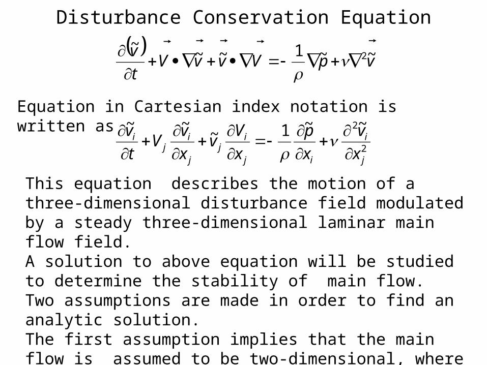
Disturbance Conservation Equation

vpVvvV

t

v

~~1~~~

2

Equation in Cartesian index notation is written as

2

2~~1~~~

j

i

ij

ij

j

ij

i

x

v

x

p

x

Vv

x

vV

t

v

This equation describes the motion of a three-dimensional disturbance field modulated by a steady three-dimensional laminar main flow field. A solution to above equation will be studied to determine the stability of main flow.Two assumptions are made in order to find an analytic solution. The first assumption implies that the main flow is assumed to be two-dimensional, where the velocity vector in streamwise direction changes only in lateral direction

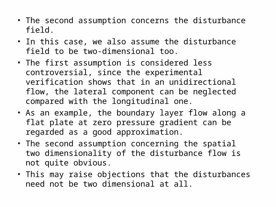
• The second assumption concerns the disturbance field.

• In this case, we also assume the disturbance field to be two-dimensional too.

• The first assumption is considered less controversial, since the experimental verification shows that in an unidirectional flow, the lateral component can be neglected compared with the longitudinal one.

• As an example, the boundary layer flow along a flat plate at zero pressure gradient can be regarded as a good approximation.

• The second assumption concerning the spatial two dimensionality of the disturbance flow is not quite obvious.

• This may raise objections that the disturbances need not be two dimensional at all.

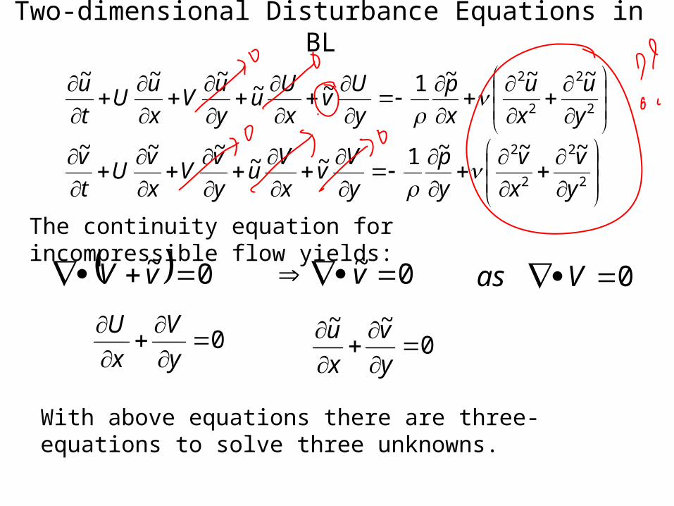
Two-dimensional Disturbance Equations in BL

2

2

2

2 ~~~1~~~~~

y

u

x

u

x

p

y

Uv

x

Uu

y

uV

x

uU

t

u

2

2

2

2 ~~~1~~~~~

y

v

x

v

y

p

y

Vv

x

Vu

y

vV

x

vU

t

v

The continuity equation for incompressible flow yields:

0~ vV

0~ v

0 Vas

0~~

y

v

x

u0

y

V

x

U

With above equations there are three-equations to solve three unknowns.

Modulation of Disturbance by BL Flow

2

2

2

2 ~~~1~~~

y

u

x

u

x

p

y

Uv

x

uU

t

u

2

2

2

2 ~~~1~~

y

v

x

v

y

p

x

vU

t

v

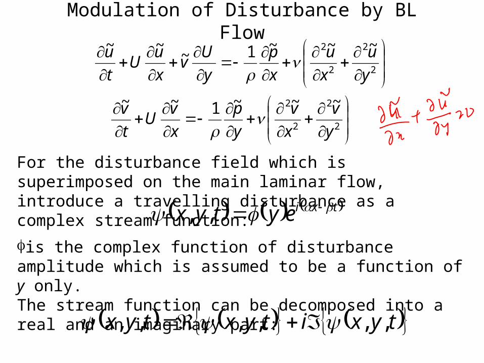
For the disturbance field which is superimposed on the main laminar flow, introduce a travelling disturbance as a complex stream function:

tyxityxtyx ,,,,,,

txieytyx ,,is the complex function of disturbance amplitude which is assumed to be a function of y only. The stream function can be decomposed into a real and an imaginary part:

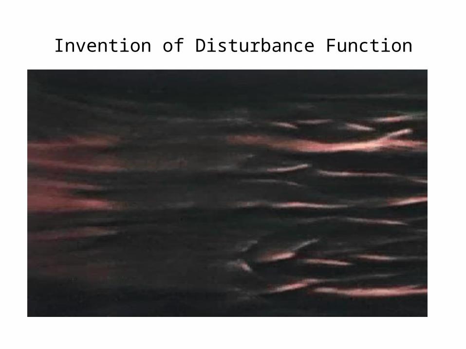
Invention of Disturbance Function

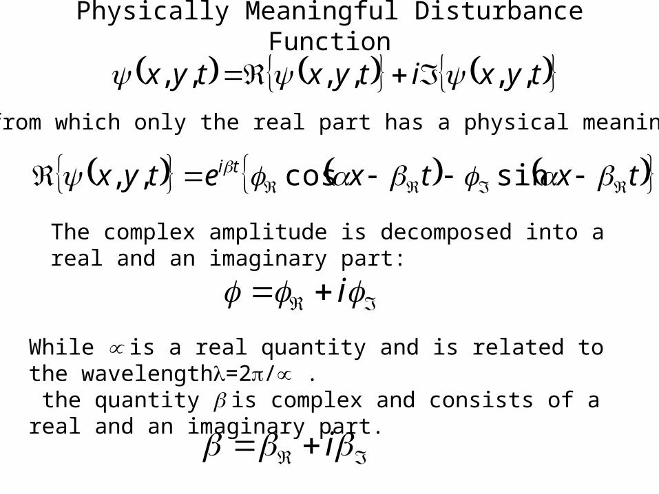
Physically Meaningful Disturbance Function

from which only the real part has a physical meaning.

tyxityxtyx ,,,,,,

The complex amplitude is decomposed into a real and an imaginary part:

i

txtxetyx ti sincos,,

While is a real quantity and is related to the wavelength=2/ . the quantity is complex and consists of a real and an imaginary part.

i

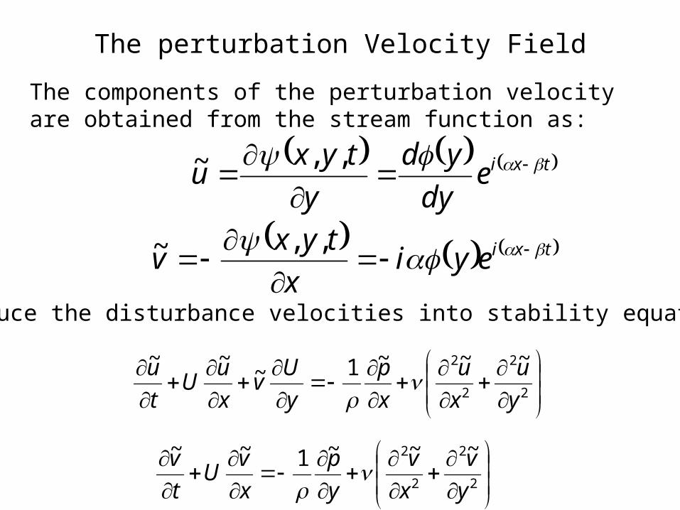
The perturbation Velocity Field

The components of the perturbation velocity are obtained from the stream function as:

txiedy

yd

y

tyxu

,,~

txieyix

tyxv

,,~

2

2

2

2 ~~~1~~~

y

u

x

u

x

p

y

Uv

x

uU

t

u

2

2

2

2 ~~~1~~

y

v

x

v

y

p

x

vU

t

v

Introduce the disturbance velocities into stability equations:

Orr-Sommerfeld -equation

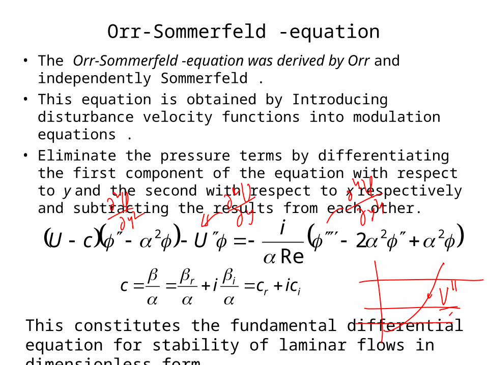
• The Orr-Sommerfeld -equation was derived by Orr and independently Sommerfeld .

• This equation is obtained by Introducing disturbance velocity functions into modulation equations .

• Eliminate the pressure terms by differentiating the first component of the equation with respect to y and the second with respect to x respectively and subtracting the results from each other.

222 2Re

i

UcU

irir iccic

This constitutes the fundamental differential equation for stability of laminar flows in dimensionless form.

Orr-Sommerfeld Eigen value Problem

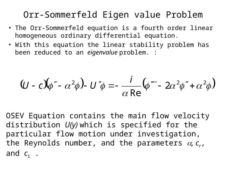
• The Orr-Sommerfeld equation is a fourth order linear homogeneous ordinary differential equation.

• With this equation the linear stability problem has been reduced to an eigenvalue problem. :

222 2Re

i

UcU

OSEV Equation contains the main flow velocity distribution U(y) which is specified for the particular flow motion under investigation, the Reynolds number, and the parameters , cr, and ci .

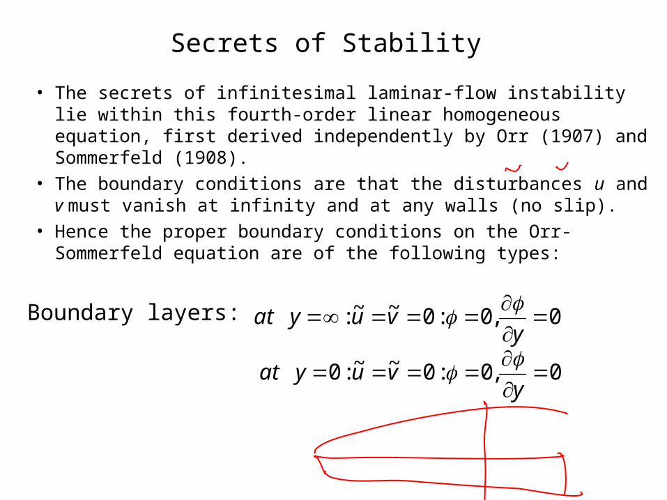
Secrets of Stability

• The secrets of infinitesimal laminar-flow instability lie within this fourth-order linear homogeneous equation, first derived independently by Orr (1907) and Sommerfeld (1908).

• The boundary conditions are that the disturbances u and v must vanish at infinity and at any walls (no slip).

• Hence the proper boundary conditions on the Orr-Sommerfeld equation are of the following types:

0,0:0~~:0

y

vuyat

0,0:0~~:

y

vuyatBoundary layers:

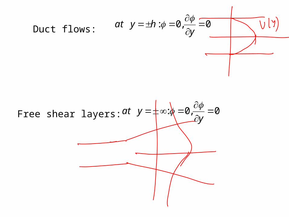
Free shear layers:

Duct flows: 0,0:

y

hyat

0,0:

y

yat

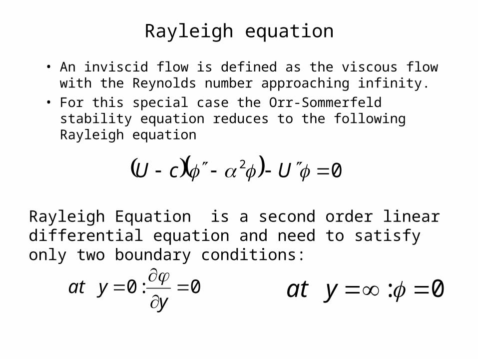
Rayleigh equation

• An inviscid flow is defined as the viscous flow with the Reynolds number approaching infinity.

• For this special case the Orr-Sommerfeld stability equation reduces to the following Rayleigh equation

02 UcU

Rayleigh Equation is a second order linear differential equation and need to satisfy only two boundary conditions:

0:0

y

yat

0: yat

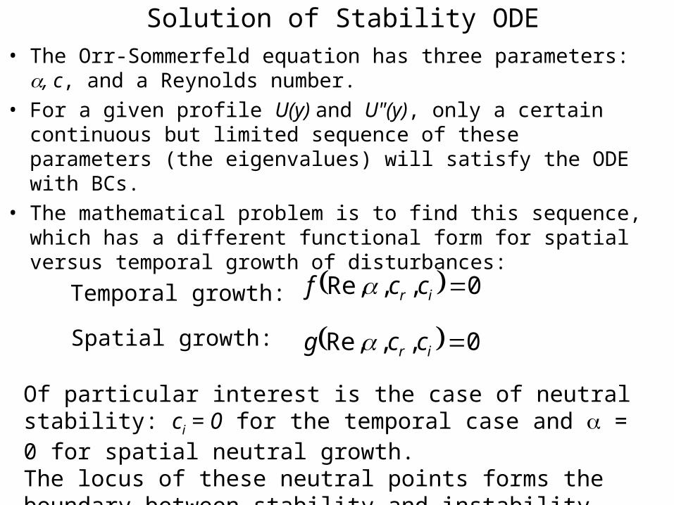
Solution of Stability ODE

• The Orr-Sommerfeld equation has three parameters: , c, and a Reynolds number.

• For a given profile U(y) and U"(y), only a certain continuous but limited sequence of these parameters (the eigenvalues) will satisfy the ODE with BCs.

• The mathematical problem is to find this sequence, which has a different functional form for spatial versus temporal growth of disturbances:

Temporal growth:

Spatial growth:

0,,Re, ir ccf

0,,Re, ir ccg

Of particular interest is the case of neutral stability: ci = 0 for the temporal case and = 0 for spatial neutral growth. The locus of these neutral points forms the boundary between stability and instability.

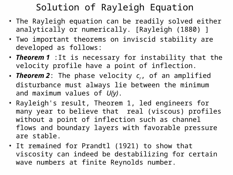
Solution of Rayleigh Equation

• The Rayleigh equation can be readily solved either analytically or numerically. [Rayleigh (1880) ]

• Two important theorems on inviscid stability are developed as follows:

• Theorem 1 :It is necessary for instability that the velocity profile have a point of inflection.

• Theorem 2: The phase velocity cr, of an amplified disturbance must always lie between the minimum and maximum values of U(y).

• Rayleigh's result, Theorem 1, led engineers for many year to believe that real (viscous) profiles without a point of inflection such as channel flows and boundary layers with favorable pressure are stable.

• It remained for Prandtl (1921) to show that viscosity can indeed be destabilizing for certain wave numbers at finite Reynolds number.

16

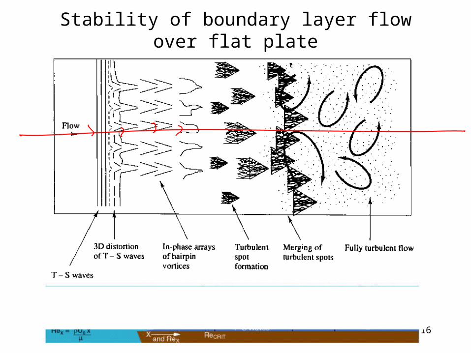
Stability of boundary layer flow over flat plate

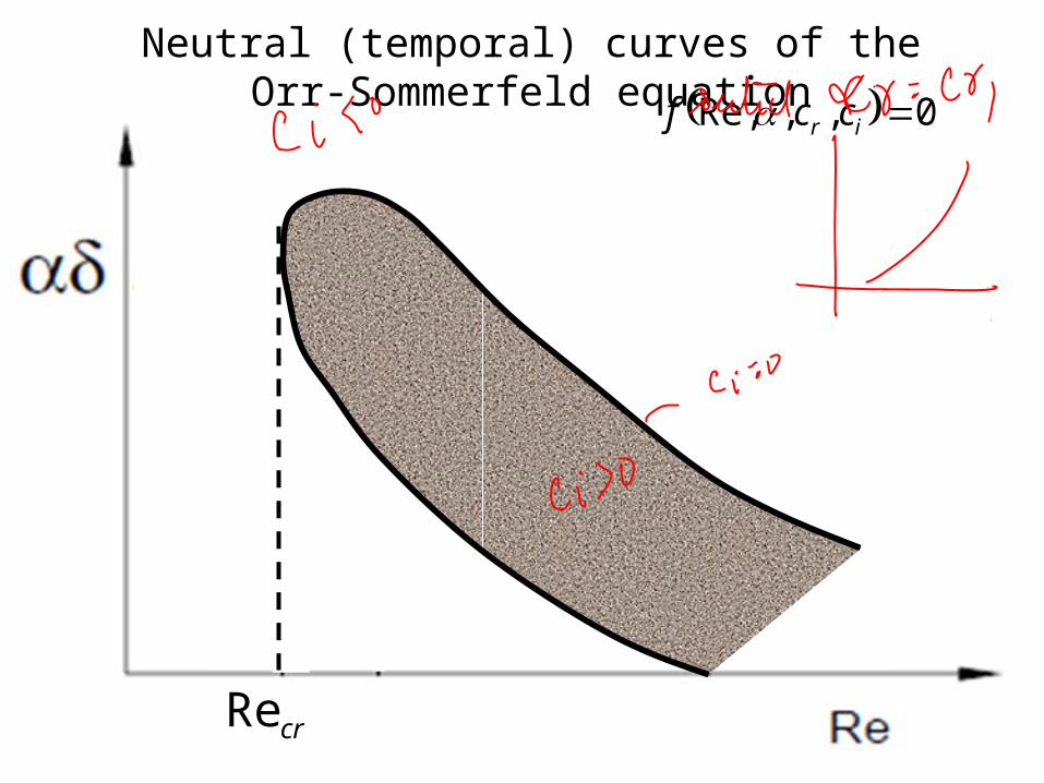
Neutral (temporal) curves of the Orr-Sommerfeld equation 0,,Re, ir ccf

crRe

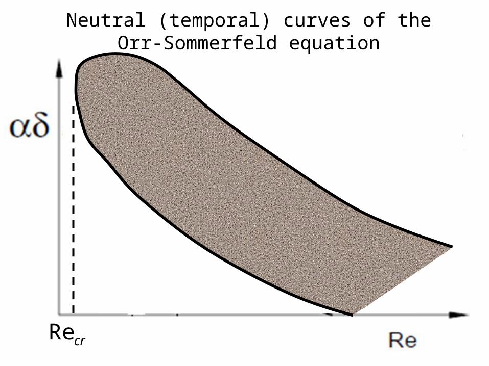
Neutral (temporal) curves of the Orr-Sommerfeld equation

crRe

Neutral (temporal) curves of the Orr-Sommerfeld equation 0,,Re, ir ccf

crRe

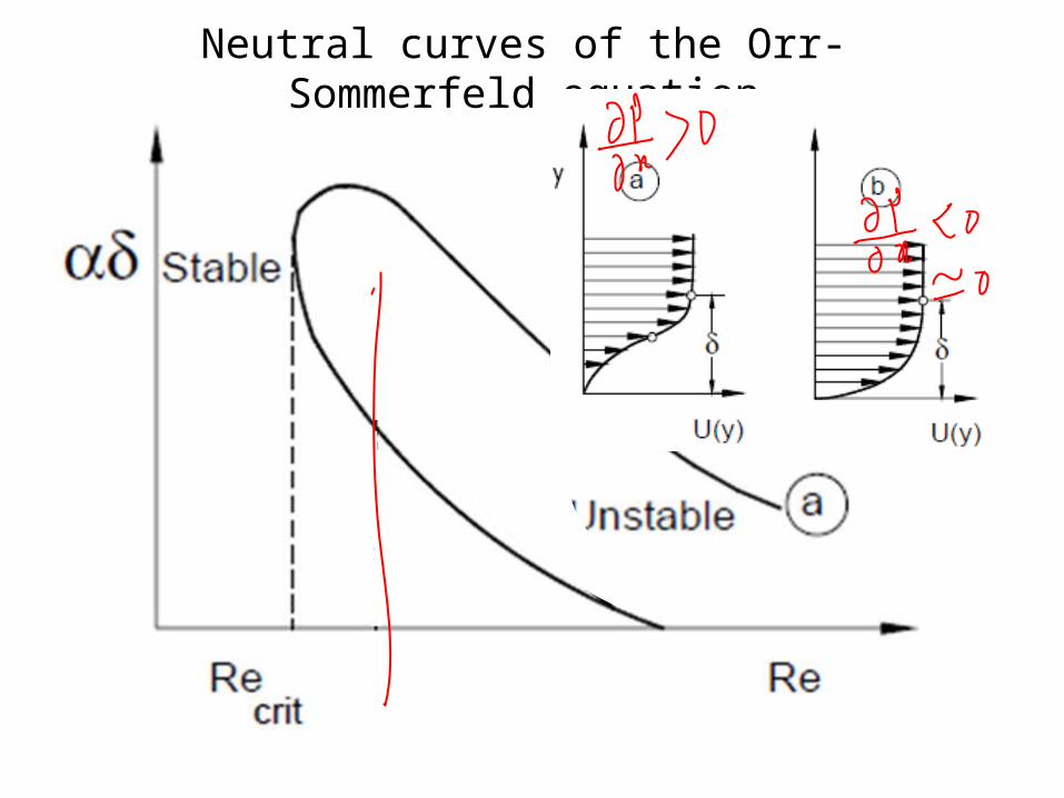
Neutral curves of the Orr-Sommerfeld equation

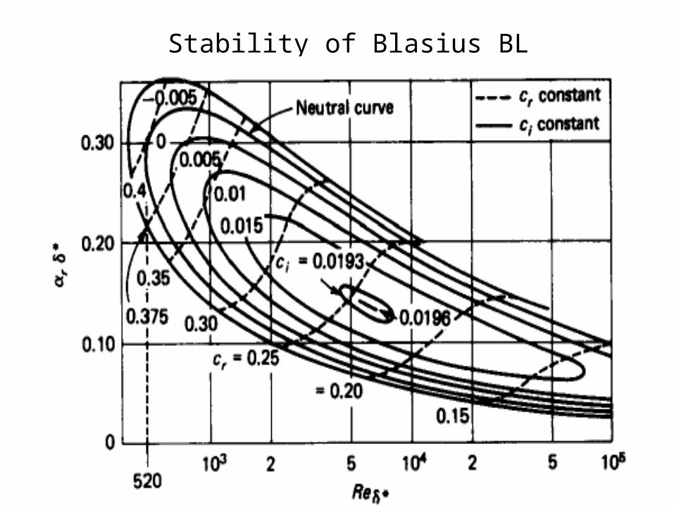
Stability of Blasius BL

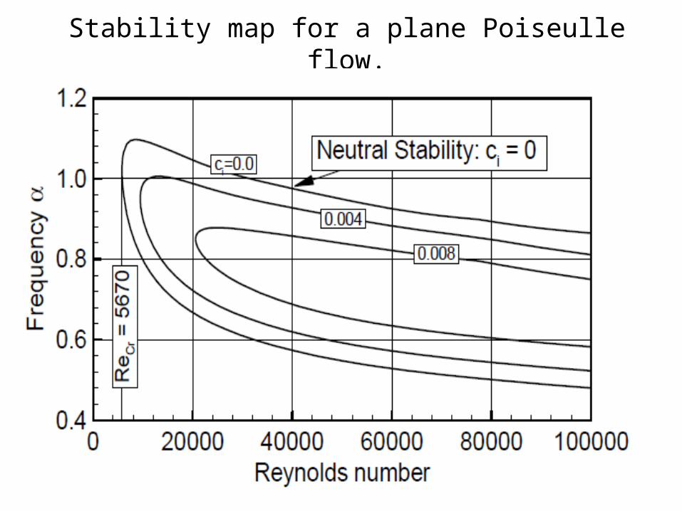
Stability map for a plane Poiseulle flow.