
Quant Base Master - Mathematical Marketing
278
M M α α t t h h e e m m a a t t i i c c a a l l M M α α r r k k e e t t i i n n g g Charles F. Hofacker New South Network Services
Transcript of Quant Base Master - Mathematical Marketing

MMααtthheemmaattiiccaall MMααrrkkeettiinngg
CChhaarrlleess FF.. HHooffaacckkeerr
New South Network Services


i
Mathematical Marketing Version NSNS.2007.08.26 Copyright © 2007 New South Network Services
Licensed under the Open Software License version 1.1
1) Grant of Copyright License. Licensor hereby grants You a world-wide, royalty-free, non-exclusive, perpetual, non-sublicenseable license to do the following:
a) to reproduce the Original Work in copies;
b) to prepare derivative works ("Derivative Works") based upon the Original Work;
c) to distribute copies of the Original Work and Derivative Works to the public, with the proviso that copies of Original Work or Derivative Works that You distribute shall be licensed under the Open Software License;
d) to perform the Original Work publicly; and
e) to display the Original Work publicly.
2) Grant of Patent License. Licensor hereby grants You a world-wide, royalty-free, non-exclusive, perpetual, non-sublicenseable license, under patent claims owned or controlled by the Licensor that are embodied in the Original Work as furnished by the Licensor ("Licensed Claims") to make, use, sell and offer for sale the Original Work. Licensor hereby grants You a world-wide, royalty-free, non-exclusive, perpetual, non-sublicenseable license under the Licensed Claims to make, use, sell and offer for sale Derivative Works.
3) Grant of Source Code License. The term "Source Code" means the preferred form of the Original Work for making modifications to it and all available documentation describing how to modify the Original Work. Licensor hereby agrees to provide a machine-readable copy of the Source Code of the Original Work along with each copy of the Original Work that Licensor distributes. Licensor reserves the right to satisfy this obligation by placing a machine-readable copy of the Source Code in an information repository reasonably calculated to permit inexpensive and convenient access by You for as long as Licensor continues to distribute the Original Work, and by publishing the address of that information repository in a notice immediately following the copyright notice that applies to the Original Work.
4) Exclusions From License Grant. Nothing in this License shall be deemed to grant any rights to trademarks, copyrights, patents, trade secrets or any other intellectual property of Licensor except as expressly stated herein. No patent license is granted to make, use, sell or offer to sell embodiments of any patent claims other than the Licensed Claims defined in Section 2. No right is granted to the trademarks of Licensor even if such marks are included in the Original Work. Nothing in this License shall be interpreted to prohibit Licensor from licensing under different terms from this License any Original Work that Licensor otherwise would have a right to license.
5) External Deployment. The term "External Deployment" means the use or distribution of the Original Work or Derivative Works in any way such that the Original Work or Derivative Works may be used by anyone other than You, whether the Original Work or Derivative Works are distributed to those persons or made available as an application intended for use over a computer network. As an express condition for the grants of license hereunder, You agree that any External Deployment by You of a Derivative Work shall be deemed a distribution and shall be licensed to all under the terms of this License, as prescribed in section 1(c) herein.

ii
6) Attribution Rights. You must retain, in the Source Code of any Derivative Works that You create, all copyright, patent or trademark notices from the Source Code of the Original Work, as well as any notices of licensing and any descriptive text identified therein as an "Attribution Notice." You must cause the Source Code for any Derivative Works that You create to carry a prominent Attribution Notice reasonably calculated to inform recipients that You have modified the Original Work.
7) Warranty and Disclaimer of Warranty. Licensor warrants that the copyright in and to the Original Work is owned by the Licensor or that the Original Work is distributed by Licensor under a valid current license from the copyright owner. Except as expressly stated in the immediately proceeding sentence, the Original Work is provided under this License on an "AS IS" BASIS and WITHOUT WARRANTY, either express or implied, including, without limitation, the warranties of NON-INFRINGEMENT, MERCHANTABILITY or FITNESS FOR A PARTICULAR PURPOSE. THE ENTIRE RISK AS TO THE QUALITY OF THE ORIGINAL WORK IS WITH YOU. This DISCLAIMER OF WARRANTY constitutes an essential part of this License. No license to Original Work is granted hereunder except under this disclaimer.
8) Limitation of Liability. Under no circumstances and under no legal theory, whether in tort (including negligence), contract, or otherwise, shall the Licensor be liable to any person for any direct, indirect, special, incidental, or consequential damages of any character arising as a result of this License or the use of the Original Work including, without limitation, damages for loss of goodwill, work stoppage, computer failure or malfunction, or any and all other commercial damages or losses. This limitation of liability shall not apply to liability for death or personal injury resulting from Licensor's negligence to the extent applicable law prohibits such limitation. Some jurisdictions do not allow the exclusion or limitation of incidental or consequential damages, so this exclusion and limitation may not apply to You.
9) Acceptance and Termination. If You distribute copies of the Original Work or a Derivative Work, You must make a reasonable effort under the circumstances to obtain the express and volitional assent of recipients to the terms of this License. Nothing else but this License (or another written agreement between Licensor and You) grants You permission to create Derivative Works based upon the Original Work or to exercise any of the rights granted in Sections 1 herein, and any attempt to do so except under the terms of this License (or another written agreement between Licensor and You) is expressly prohibited by U.S. copyright law, the equivalent laws of other countries, and by international treaty. Therefore, by exercising any of the rights granted to You in Sections 1 herein, You indicate Your acceptance of this License and all of its terms and conditions. This License shall terminate immediately and you may no longer exercise any of the rights granted to You by this License upon Your failure to honor the proviso in Section 1(c) herein.
10) Mutual Termination for Patent Action. This License shall terminate automatically and You may no longer exercise any of the rights granted to You by this License if You file a lawsuit in any court alleging that any OSI Certified open source software that is licensed under any license containing this "Mutual Termination for Patent Action" clause infringes any patent claims that are essential to use that software.
11) Jurisdiction, Venue and Governing Law. Any action or suit relating to this License may be brought only in the courts of a jurisdiction wherein the Licensor resides or in which Licensor conducts its primary business, and under the laws of that jurisdiction excluding its conflict-of-law provisions. The application of the United Nations Convention on Contracts for the International Sale of Goods is expressly excluded. Any use of the Original Work outside the scope of this License or after its termination shall be subject to the requirements and penalties of the U.S.

iii
Copyright Act, 17 U.S.C. § 101 et seq., the equivalent laws of other countries, and international treaty. This section shall survive the termination of this License.
12) Attorneys Fees. In any action to enforce the terms of this License or seeking damages relating thereto, the prevailing party shall be entitled to recover its costs and expenses, including, without limitation, reasonable attorneys' fees and costs incurred in connection with such action, including any appeal of such action. This section shall survive the termination of this License.
13) Miscellaneous. This License represents the complete agreement concerning the subject matter hereof. If any provision of this License is held to be unenforceable, such provision shall be reformed only to the extent necessary to make it enforceable.
14) Definition of "You" in This License. "You" throughout this License, whether in upper or lower case, means an individual or a legal entity exercising rights under, and complying with all of the terms of, this License. For legal entities, "You" includes any entity that controls, is controlled by, or is under common control with you. For purposes of this definition, "control" means (i) the power, direct or indirect, to cause the direction or management of such entity, whether by contract or otherwise, or (ii) ownership of fifty percent (50%) or more of the outstanding shares, or (iii) beneficial ownership of such entity.
15) Right to Use. You may use the Original Work in all ways not otherwise restricted or conditioned by this License or by law, and Licensor promises not to interfere with or be responsible for such uses by You.
This license is Copyright (C) 2002 Lawrence E. Rosen. All rights reserved. Permission is hereby granted to copy and distribute this license without modification. This license may not be modified without the express written permission of its copyright owner. License Addendum. Names of contributors must be prominently featured in any use of this or derivative works.

iv
To Linda Susan Vaughn, La Dolcissima

v
Table of Contents
Preface ........................................................................................................................................... xi
Prerequisite Structure................................................................................................................ xii
Acknowledgments..................................................................................................................... xiii
Section I: Mathematical Fundamentals ............................................................. 1
Chapter 1: Linear Algebra....................................................................................... 2 1.1 Introduction to Vector and Matrix Notation........................................................................... 2 1.2 The First Steps Towards an Algebra for Matrices.................................................................. 3 1.3 Matrix Multiplication ............................................................................................................. 7 1.4 Partitioned Matrices .............................................................................................................. 8 1.5 Cross-Product Matrices .......................................................................................................... 9 1.6 Properties of Matrix Multiplication...................................................................................... 10 1.7 The Trace of a Square Matrix............................................................................................... 11 1.8 The Determinant of a Matrix................................................................................................ 11 1.9 The Inverse of a Matrix ........................................................................................................ 12 1.10 Kronecker Product.............................................................................................................. 13 References .................................................................................................................................. 13
Chapter 2: Descriptive Statistics ...................................................................... 14 2.1 Review of Univariate Statistics ............................................................................................ 14 2.2 Matrix Expressions for Descriptive Statistics....................................................................... 15
Chapter 3: Calculus Tools ...................................................................................... 20 3.1 Logarithms and Exponents ................................................................................................... 20 3.2 A Review of Scalar Calculus................................................................................................ 20 3.3 The Scalar Function of a Vector.......................................................................................... 22 3.4 Derivative of Multiple Functions with Respect to a Vector ................................................. 23 3.5 Eigen Structure for Symmetric Matrices .............................................................................. 24 3.6 A Small Example Calculating the Eigenvalue and Eigenvector........................................... 26 3.7 Some Properties of Eigenstructure ....................................................................................... 28 3.8 Some Geometric Aspects of Eigenstructure ......................................................................... 30 3.9 Linear and Nonlinear Parameter Estimation......................................................................... 30 3.10 Maximum Likelihood Parameter Estimation...................................................................... 32 References .................................................................................................................................. 34
Chapter 4: Distributions .......................................................................................... 36 4.1 The Algebra of Expectations and Variances ........................................................................ 36 4.2 The Normal Distribution ...................................................................................................... 37 4.3 The Multivariate Normal Distribution.................................................................................. 40 4.4 Chi Square ............................................................................................................................ 41 4.5 Cochran's Theorem............................................................................................................... 43 4.6 Student's t-Statistic ............................................................................................................... 43 4.7 The F Distribution ................................................................................................................ 45

vi
Section II: The General Linear Model.............................................................. 46
Chapter 5: Ordinary Least Squares ............................................................... 48 5.1 The Regression Model.......................................................................................................... 48 5.2 Least Squares Estimation ..................................................................................................... 48 5.3 What Do We Mean by a Good Statistic?.............................................................................. 51 5.4 Maximum Likelihood Estimation of Regression Parameters .............................................. 52 5.5 Sums of Squares of the Regression Model ........................................................................... 54 5.6 The Covariance Estimator for β ........................................................................................... 55 5.7 Regression with Z-Scores..................................................................................................... 56 5.8 Partialing Variance ............................................................................................................... 57 5.9 The Intercept-Only Model................................................................................................... 58 5.10 Response Surface Models................................................................................................... 60 References .................................................................................................................................. 62
Chapter 6: Testing Linear Hypotheses ....................................................... 64 6.1 The Distribution of the Regression Model Estimator........................................................... 64 6.2 A 1 - α Confidence Interval ................................................................................................ 66 6.3 Statistical Hypothesis Testing .............................................................................................. 66 6.4 More Complex Hypotheses and the t-statistic ...................................................................... 67 6.5 Multiple Degree of Freedom Hypotheses............................................................................. 68 6.6 An Alternative Method to Estimate Sums of Squares for an Hypothesis............................. 70 6.7 The Impact of All the Independent Variables....................................................................... 70 6.8 Generalized Least Squares ................................................................................................... 72 6.9 Symmetric and Idempotent Matrices in Least Squares ........................................................ 73 References .................................................................................................................................. 75
Chapter 7: The Analysis of Variance ............................................................ 76 7.1 History and Overview of ANOVA....................................................................................... 76 7.2 Effect Coding ....................................................................................................................... 77 7.3 Dummy Coding .................................................................................................................... 78 7.4 Orthogonal Coding ............................................................................................................... 79 7.5 Interactive Effects................................................................................................................. 80 7.6 Quantitative Independent Variables ..................................................................................... 82 7.7 Repeated Measures Analysis of Variance ............................................................................ 83 7.8 A Classic Repeated Measures Example ............................................................................... 84 References .................................................................................................................................. 85
Chapter 8: The Multivariate General Linear Model ........................ 86 8.1 Introduction ......................................................................................................................... 86 8.2 Testing Multiple Hypotheses............................................................................................... 86 8.4 Union-Intersection Protection from Post Hoc Hypotheses.................................................. 88 8.5 Details About the Trace Operator and It's Derivative ......................................................... 89 8.6 The Kronecker Product ....................................................................................................... 90 8.7 The Vec Operator ................................................................................................................ 91 8.8 Eigenstructure for Asymmetric Matrices ............................................................................ 91 8.9 Eigenstructure for Rectangular Matrices ............................................................................. 91 8.10 The Multivariate General Linear Model............................................................................ 92 8.11 A Least Squares Estimator for the MGLM........................................................................ 93 8.12 Properties of the Error Matrix ε......................................................................................... 94

vii
8.13 Properties of the B Matrix .................................................................................................. 94 8.14 The Multivariate General Linear Hypothesis ..................................................................... 95 8.15 Some Examples of MGLM Hypotheses ............................................................................ 95 8.16 Hypothesis and Error Sums of Squares and Cross-Products .............................................. 96 8.17 Statistics for Testing the Multivariate General Linear Hypothesis..................................... 97 8.18 Canonical Correlation......................................................................................................... 99 8.19 MANOVA........................................................................................................................ 101 8.20 MANOVA and Repeated Measures ................................................................................. 101 8.21 Classification.................................................................................................................... 104 8.22 Multiple Group Discriminant Function ............................................................................ 107 References ................................................................................................................................ 108
Section III: Covariance Structure ...................................................................... 109
Chapter 9: Confirmatory Factor Analysis............................................... 110 9.1 The Confirmatory Factor Analysis Model......................................................................... 110 9.2 A Confirmatory Factor Analysis Example ........................................................................ 112 9.3 Setting a Metric for Latent Variables ................................................................................ 114 9.4 Degrees of Freedom for a Confirmatory Factor Analysis Model ...................................... 115 9.5 Maximum Likelihood Estimators for Factor Analysis ...................................................... 115 9.6 Special Case: The One Factor Model ................................................................................ 117 9.7 The Multi-Trait Multi-Method Model................................................................................ 118 References ................................................................................................................................ 122
Chapter 10: Structural Equation Models ................................................. 124 10.1 The Basic Structural Equation Model .............................................................................. 124 10.2 A Simple Example with Four Variables........................................................................... 126 10.3 All y Models..................................................................................................................... 127 10.4 In What Sense Are These Causal Models?....................................................................... 128 10.5 Regression As a Structural Equation Model..................................................................... 129 10.6 Recursive and Nonrecursive Models................................................................................ 130 10.7 Structural Equation Models with Latent Variables........................................................... 130 10.8 Second Order Factor Analysis.......................................................................................... 133 10.9 Models with Structured Means......................................................................................... 134 References ................................................................................................................................ 135
Chapter 11: Exploratory Factor Analysis................................................ 136 11.1 Some Comments on the History of Factor Analysis......................................................... 136 11.2 Principal Factors Factor Extraction .................................................................................. 136 11.3 Exploratory Factor Analysis Is a Special Case of Confirmatory...................................... 139 11.4 Other Methods of Factor Extraction................................................................................. 140 11.5 Factor Rotation ................................................................................................................. 140 11.6 Oblique Rotation .............................................................................................................. 143 References ................................................................................................................................ 144
Section IV: Consumer Judgment and Choice............................................ 145
Chapter 12: Judgment and Choice ............................................................. 146 12.1 Historical Antecedents ..................................................................................................... 146 12.2 A Simple Model for Detecting Something ....................................................................... 148

viii
12.3 Thurstone’s Law of Comparative Judgment..................................................................... 150 12.4 Estimation of the Parameters in Thurstone’s Case III: Least Squares and ML ............... 153 12.5 The Law of Categorical Judgment.................................................................................... 157 12.6 The Theory of Signal Detectability .................................................................................. 159 12.7 Functional Measurement .................................................................................................. 164 References ................................................................................................................................ 164
Chapter 13: Random Utility Models............................................................. 168 13.1 Some Terminology and a Simple Example ...................................................................... 168 13.2 Aggregate Data................................................................................................................. 173 13.3 Weighted Least Squares and Aggregate Data .................................................................. 175 13.4 Maximum Likelihood and Disaggregate Data.................................................................. 178 13.5 Three or More Choice Options......................................................................................... 180 13.6 A Transportation Example of the MNL Model ................................................................ 181 13.7 Other Choice Models........................................................................................................ 182 13.8 Elasticities and the MNL Model....................................................................................... 184 13.9 Independence of Irrelevant Alternatives........................................................................... 185 13.10 The Polytomous Probit Model........................................................................................ 186 References ................................................................................................................................ 187
Chapter 14: Nonmetric Scaling ....................................................................... 190 14.1 Additive Conjoint Measurement ...................................................................................... 190 14.2 Multidimensional Scaling................................................................................................. 192 14.3 Other Distance Models ..................................................................................................... 194 14.4 Individual Differences in Perception................................................................................ 195 14.5 Preference Models: The Vector Model ............................................................................ 197 14.6 Preference Models: The Ideal Point Model ...................................................................... 199 References ................................................................................................................................ 190
Chapter 15: Stochastic Choice ......................................................................... 204 15.1 Key Terminology ............................................................................................................. 204 15.2 The Brand Switching Matrix ............................................................................................ 204 15.3 The Zero-Order Homogeneous Bernoulli Model ............................................................. 205 15.4 Population Heterogeneity and The Zero-Order Bernoulli Model..................................... 206 15.5 Markov Chains ................................................................................................................. 209 15.6 Learning Models............................................................................................................... 211 15.7 Purchase Incidence ........................................................................................................... 213 15.8 The Negative Binomial Distribution Model ..................................................................... 215 References ................................................................................................................................ 216
Section V: Economics and Econometrics ...................................................... 218
Chapter 16: Microeconomics ............................................................................ 220 16.1 The Notion of Elasticity ................................................................................................... 220 16.2 Optimizing the Pricing Decision ...................................................................................... 222 References ................................................................................................................................ 223
Chapter 17: Econometrics ................................................................................... 224 17.1 The Problems with Nonrecursive Systems ....................................................................... 224 17.2 Two Stage Least Squares.................................................................................................. 225

ix
17.3 Econometric Approaches to Measurement Error.............................................................. 226 17.4 Generalized Least Squares ............................................................................................... 228 17.5 Autocorrelated Error............................................................................................................. 230 17.7 Lagged Variables ................................................................................................................. 234 17.8 Partial Adjustment by Consumers .......................................................................................... 237 17.9 Adaptive Adjustment by Consumers ...................................................................................... 237 17.10 Pooling Time Series and Cross Section Data ......................................................................... 238 References.................................................................................................................................. 240
Chapter 18: Time Series .................................................................................... 242 18.1 Stationary Data Series ...................................................................................................... 242 18.2 A Linear Model for Time Series ...................................................................................... 243 18.3 Moving Average Processes .............................................................................................. 245 18.4 Autoregressive Processes ................................................................................................. 248 18.5 Details of the Algebra of the Backshift Operator ............................................................. 251 18.6 The AR(2) Process ........................................................................................................... 252 18.7 The General AR(p) Process.............................................................................................. 252 18.8 The ARMA(1,1) Mixed Process....................................................................................... 253 18.9 The ARIMA(1,1,1) Model ............................................................................................... 254 18.10 Seasonality ..................................................................................................................... 255 18.11 Identifying ARIMA(p,d,q) Models ................................................................................ 255 References ................................................................................................................................ 256
Appendices...................................................................................................................... 257
A. The Greek Alphabet .......................................................................................................... 257
Index ........................................................................................................................................... 258

x
Charles Hofacker College of Business
Florida State University Tallahassee, FL 32306-1110
+1 850 644 7864 [email protected]

xi
Preface to Version NSNS.2007.08.26 Over the years I have taught two different doctoral level quantitative methods courses in Marketing at Florida State University. The nature of these two courses changed somewhat from time to time depending on the exact offering of courses by other departments such as the Statistics Department and the Educational Measurement Department, as well as the needs of each particular cohort of students. The upshot was that I eventually ended up with a set of notes covering a good number of the most important mathematical tools used in marketing; perhaps enough material for two and a half semesters worth of classes. This manuscript is the result of transcribing most of those notes into book form. There are generally two sorts of textbooks available for a Marketing Ph D quantitative methods course. The first sort is generally user-friendly, but with little or no actual mathematics. This kind of book generally treats each presented statistical procedure as a black box. The student is taught what type of stuff to put into the box, what type of stuff is likely to come out of the box, and how to write it up. The second sort of book is journal article quality "raw material"; very technical and prone to assuming that the student has had numerous recent courses in mathematical statistics. Diving into the second type of text can be daunting. What's more, since the tradition in mathematical marketing borrows from psychology, economics and management science, no single technical book tends to cover everything and a thorough coverage of the field requires that the student jump from one set of notational conventions to another. Yet if you pick up any issue of Marketing Science or the Journal of Marketing Research, the author is liable to assume you are familiar with anything from repeated measures ANOVA to efficient parameter estimation in econometric models. This book is my attempt to create a text designed to allow students to follow the mathematical reasoning used in Marketing Science, Journal of Marketing Research and other quantitatively oriented journals. As such, it does not hide the mathematics, but it does not assume that the student already has an extensive background in mathematics. One unusual feature of this book is the license agreement, which is inspired by open source software. Although software development is a different kind of intellectual activity from book writing, the two are perhaps similar enough that methods that have worked in the former domain will also work in the latter. We shall see, but one way or the other I believe it will be interesting experiment. It occurs to me that a fairly esoteric course like PhD quantitative methods is an ideal laboratory for an open source book. I envision a community of adopters around the world adding to this version, improving it, adding teaching notes, exercises, data sets, more references, improved slides, even new chapters. There are a variety of chapters that might be useful: Bayesian techniques and Proportional Hazards models are two examples. In addition, there are many topics that could be added to individual chapters.

xii
Prerequisite Structure
Chapter Chapter Prereq Calculus Distributions Eigen structure
Esimation, ML
1 2 1 3 1 4 1
5 1, 2 3.1, 3.2, 3.3 4.1, 4.2 6 5 7 6 8 7 3.4 3.5 - 3.8
9 5 4.3 3.9, 3.10 10 9 11 9 3.5 - 3.8
12 5, 6.8 3.9, 3.10 13 12.1 - 12.4 14 7 3.9 15 5 3.9, 3.10
16 5 17 6 3.5 - 3.8 18 5
Much of what Ph D students learn about substantive issues in marketing can be studied in any order. It is, however, in the nature of technical topics that the sequence of study must be more carefully arranged. With that in mind, the above is a suggested prerequisite sequence for each chapter. The prerequisites are repeated in the beginning of each chapter. You will note that the Chapter on OLS, Chapter 5, is needed for almost everything else in the book. One could follow a sequence of Chapters 1 and 2, Sections 3.1, 3.2, 3.3, 4.1 and 4.2, Chapter 5 and then do almost any subset of chapters as a specialized course. For example, a course in LISREL modeling would go from Chapter 5 to Sections 3.9, 3.10 and 4.3 into Chapters 9 and 10. A course oriented more towards choice modeling would start out the same up to Chapter 5 to but then cover Sections 3.9, 3.10 and 6.8 followed by Chapters 12 and 13. A course oriented more towards econometrics might start with the sequence leading up to Chapter 5 and then do Chapter 6, Sections 3.5 - 3.8 on eigenstructrure and 16, 17and 18. Many other possibilities exist.

xiii
Acknowledgments I now officially dedicate this version of the book to the following: my wife and some other people and stuff. The list of other people begins with statistics professors I have had, whose opinions and ways of explanation are mixed into the chapters that follow: Don Butler, Sam Pineau, Tom Wickens, Eric Holman, Art Woodward, Peter Bentler, Andrew Comrey, Bengt Muthèn and Ed Leamer. It extends to Sandeep Krisnamurthy for bringing open source to the attention of academic marketing. E addesso, dei ringraziamenti in Italiano. Innanzi tutto a Sandro Castaldo e l’Università Bocconi. Alla Roma per vincere lo scudetto nel 2001. Per la cucina Italiana. Per quella strada a lungo del crinale vicino a Fiesole. Alla gente che stanno ripristinando le colonne del Tempio di Adriano (oggi la Borsa di Roma). Per Salvatore Zappalà perchè si fermò ad aiutarmi un pomeriggio autunale nel 2001. A Luca Debenedittis per essere il più bravo insegnante d'Italiano che abbia mai conosciuto. A Rafaele Desantis per aspettarmi dopo le discese. Per il suono che fanno la ali degli uccelli. Per la luna vista di giorno. La colonna Sonora del film La Finestra Di Fronte. Alle bici in titanio. Spero di non confondere il mondo troppo. Charles F Hofacker August 28, 2007


1
Section I: Mathematical Fundamentals

2 Chapter 1
Chapter 1: Linear Algebra
1.1 Introduction to Vector and Matrix Notation Much of the mathematical reasoning in all of the sciences that pertain to humans is linear in nature, and linear equations can be greatly condensed by matrix notation and matrix algebra. In fact, were it not for matrix notation, some equations could fill entire pages and defy our understanding. The first step in creating easier-to-grasp linear equations is to define the vector. A vector is defined as an ordered set of numbers. Vectors are classified as either row vectors or column vectors. Note that a vector with one element is called a scalar. Here are two examples. The vector a is a column vector with m elements,
⎥⎥⎥⎥
⎦
⎤
⎢⎢⎢⎢
⎣
⎡
=
m
2
1
a
aa
La ,
and the vector b is a row vector with q elements: ]bbb[ q21 L=b . You should notice that in this text vectors are generally represented with lower case letters in bold. There are a variety of ways that we can operate on vectors, but one of the simplest is the transpose operator, which, when applied to a vector, turns a row into a column and vice versa. For example, ].aaa[ m21 L=′a By convention, in this book, a vector with a transpose will generally imply that we are dealing with a row. The implication is that by default, all vectors are columns. A matrix is defined as a collection of vectors, for example
.x
xxx
xxx
xxx
ij
nm2n1n
m22221
m11211
=
⎥⎥⎥⎥⎥⎥
⎦
⎤
⎢⎢⎢⎢⎢⎢
⎣
⎡
=
L
LLLL
L
L
X
In this text, matrices are typically represented with an upper case bold letter. The square brackets are used to list all of the elements of a matrix while the curly brackets are sometimes used to show a typical element of the matrix and thereby symbolize the entire matrix in that manner. Note that the first subscript of X indexes the row, while the second indexes columns. Matrices are characterized by their order, that is to say, the number of rows and columns that they have. The above matrix X is of order n by m, sometimes written n · m. From time to time we may see a matrix like X written with its order like so: nXm. It is semantically appropriate to say that a row vector is a matrix of but one row, and a column vector is a matrix of one column. Of course, a scalar can be thought of as the special case when we have a 1 by 1 matrix.

Linear Algebra 3
At times it will prove useful to keep track of the individual vectors that comprise a matrix. Suppose, for example that we defined each of the rows of X as
]xxx[
]xxx[]xxx[
nm2n1nn
m222212
m112111
L
LL
L
L
=′==′=′
⋅
⋅
⋅
x
xx
and then defined each column of X:
⎥⎥⎥⎥⎥⎥
⎦
⎤
⎢⎢⎢⎢⎢⎢
⎣
⎡
=
⎥⎥⎥⎥⎥⎥
⎦
⎤
⎢⎢⎢⎢⎢⎢
⎣
⎡
=
⎥⎥⎥⎥⎥⎥
⎦
⎤
⎢⎢⎢⎢⎢⎢
⎣
⎡
= ⋅⋅⋅
nm
m2
m1
m
2n
22
12
2
1n
21
11
1
x
x
x
,,
x
x
x
,
x
x
x
LL
LLxxx (1.1)
so that X could be represented as
[ ]m
n
⋅⋅⋅
⋅
⋅
⋅
=
⎥⎥⎥⎥
⎦
⎤
⎢⎢⎢⎢
⎣
⎡
′
′′
= xxx
x
xx
X LL 21
2
1
. (1.2)
In this context, the dot is known as a subscript reduction operator since it allows us to aggregate over the subscript replaced by the dot. So for example, the dot in ⋅′ix summarizes all of the columns in the ith row of X. Every so often a matrix will have exactly as many rows as columns, in which case it is a square matrix. Many matrices of importance in statistics are in fact square.
1.2 The First Steps Towards an Algebra for Matrices One of the first steps we need to make to create an algebra for matrices is to define equality. We now do so defining two matrices A = B iff aij = bij for all i, j. (1.3) Every element of A and B needs to be identical. For this to be possible, obviously both A and B must have the same order! Just as one can transpose a vector, a matrix can be transposed as well. Matrix transposition takes all rows into columns and vice versa. For example,
⎥⎦
⎤⎢⎣
⎡=
′
⎥⎥⎥
⎦
⎤
⎢⎢⎢
⎣
⎡
512443
541423
.
Bringing our old friend X back, we could say that

4 Chapter 1
[ ].
xxx
xxxxxx
n21
m
2
1
nmm2m1
2n2212
1n2111
⋅⋅⋅
⋅
⋅
⋅
=
⎥⎥⎥⎥
⎦
⎤
⎢⎢⎢⎢
⎣
⎡
′
′′
=
⎥⎥⎥⎥
⎦
⎤
⎢⎢⎢⎢
⎣
⎡
=′
xxx
x
xx
X
LL
L
LLLL
L
L
We might add that ( ) XX =′′ . (1.4) A square matrix S is called symmetric if SS ′= . (1.5) Of course, a scalar, being a 1 by 1 matrix, is always symmetric. Now we are ready to define matrix addition. For two matrices A and B of the same order, their sum is defined as the addition of each corresponding element as in
.bac ijijij +=
+= BAC (1.6)
That is to say, we take each element of A and B and add them to produce the corresponding element of the sum. Here it must be emphasized that matrix addition is only possible if the components are conformable for addition. In order to be conformable for addition, they must have the same number of rows and columns. It is possible to multiply a scalar times a matrix. This is called, appropriately enough, scalar multiplication. If c is a scalar, we could have cA = B. For example we might have
⎥⎥⎥⎥
⎦
⎤
⎢⎢⎢⎢
⎣
⎡
⋅⋅
⋅⋅
⋅⋅
=
⎥⎥⎥⎥
⎦
⎤
⎢⎢⎢⎢
⎣
⎡
3231
2221
1211
3231
2221
1211
acac
acac
acac
aa
aa
aa
c .
Assuming that c1 and c2 are scalars, we can outline some properties of scalar multiplication: Associative: c1(c2 A) = (c1c2) A (1.7)

Linear Algebra 5
Distributive: (c1 + c2) A = c1 A + c2 A (1.8) Now that we have defined matrix addition and scalar multiplication, we can define matrix subtraction as BABA )1(−+=− . There are a few special matrices that will be of use later that have particular names. For example, an n by m matrix filled with zeroes is called a null matrix,
⎥⎥⎥⎥⎥⎥
⎦
⎤
⎢⎢⎢⎢⎢⎢
⎣
⎡
=
000
000
000
mn
L
LLLL
L
L
0 (1.9)
and an n · m matrix of ones is called a unit matrix:
⎥⎥⎥⎥⎥⎥
⎦
⎤
⎢⎢⎢⎢⎢⎢
⎣
⎡
=
111
111
111
mn
L
LLLL
L
L
1 . (1.10)
We have already seen that a matrix that is equal to its transpose ( SS ′= ) is referred to as symmetric. A diagonal matrix, such as D, is a special case of a symmetric matrix such that
⎥⎥⎥⎥⎥⎥
⎦
⎤
⎢⎢⎢⎢⎢⎢
⎣
⎡
=
mm
22
11
d00
0d0
00d
L
LLLL
L
L
D . (1.11)
i. e. the matrix consists of zeroes in all of the off-diagonal positions. In contrast, the diagonal positions hold elements for which the subscripts are identical. A special case of a diagonal matrix is called a scalar matrix, a typical example of which appears below:
⎥⎥⎥⎥⎥⎥
⎦
⎤
⎢⎢⎢⎢⎢⎢
⎣
⎡
c00
0c0
00c
L
LLLL
L
L
. (1.12)
And finally, a special type of scalar matrix is called the identity matrix. As we will soon see, the identity matrix serves as the identity element of matrix multiplication. For now, note that we generally use the symbol I to refer to such a matrix:

6 Chapter 1
⎥⎥⎥⎥
⎦
⎤
⎢⎢⎢⎢
⎣
⎡
=
100
010001
L
LLLL
L
L
I .
Having defined the identity matrix, we can think of a scalar matrix as being expressible as cI where c is a scalar. We can now define some properties of matrix addition. Commutative: A + B = B + A (1.13) Associative: A + (B + C) = (A + B) + C (1.14) Identity: A + 0 = A (1.15) Note that in the definitions above we have assumed that all matrices are conformable for addition. At this point we are ever closer to having all of the tools we need to create an algebra with vectors and matrices. We are only missing a way to multiply vectors and matrices. We now turn to that task. Assume we have a 1 by m row vector, a', and an m by 1 column vector, b. In that case, we can have
[ ]
.ba
bababa
b
bb
aaa
m
1iii
mm2211
m
2
1
m21
∑=
=
+++=
⎥⎥⎥⎥
⎦
⎤
⎢⎢⎢⎢
⎣
⎡
=′
L
LLba
(1.16)
This operation is called taking a linear combination, but it is also known as the scalar product, the inner product, and the dot product. This is an extremely useful operation and a way to express a linear function with a very dense notation. For example, to sum the elements of a vector, we need only write
[ ] ∑=⎥⎥⎥⎥
⎦
⎤
⎢⎢⎢⎢
⎣
⎡
=′n
ii
m
2
1
a
a
aa
111L
La1 .
When a linear combination of two non-null vectors equals zero, we say that they are orthogonal as x′ and y below: 0=′yx . (1.17) Geometrically, this is equivalent to saying that they are at right angles in a space with as many axes as there are elements in the vector. Assume for example that we have a 2 element vector. This can be interpreted as a point, or a vector with a terminus, in a plane (a two space). Consider the graph below:

Linear Algebra 7
Note that the vector [ ]12=′x is represented in the graph. Can you picture an orthogonal vector? The
length of a vector is given by ∑=′ 2ixxx .
1.3 Matrix Multiplication The main difference between scalar and matrix multiplication, a difference that can really throw off students, is that the commutative property does not apply in matrix multiplication. In general, AB ≠ BA, but what’s more, BA may not even be possible. We shall see why in a second. For now, note that in the product AB, where A is m · n and B is n · p, we would call A the premultiplying matrix and B the postmultiplying matrix. Each row of A is combined with each column of B in vector multiplication. An element of the product matrix, cij, is produced from the ith row of A and the jth column of B. In other words,
∑=′= ⋅⋅
n
kkjikjiij bac ba (1.18)
The first thing we should note here is that the row vectors of A must be of the same order as the column vectors of B, in our case of order n. If not, A and B would not be conformable for multiplication. We could diagram things like this:
Here the new matrix C takes on the number of rows of A and the number of columns of B. The number of columns of A must match the number of rows of B. OK, now let’s look at a quick example. Say
-2
-1
0
1
2
-2 -1 0 1 2
x′ =[2 1]
pnnmpm BAC =

8 Chapter 1
.85133
2)1(4)0(3)2(1)1(1)0(2)2(2)2(4)3(3)1(1)2(1)3(2)1(
214132
102231
⎥⎦
⎤⎢⎣
⎡=
⎥⎦
⎤⎢⎣
⎡++++++−++−
=
⎥⎥⎥
⎦
⎤
⎢⎢⎢
⎣
⎡
⎥⎦
⎤⎢⎣
⎡−=C
A particular triple product, with a premultiplying row vector, a square matrix, and a postmultiplying column vector, is known as a bilinear form: 1mmmm111 dBac ′= (1.19) A very important special case of the bilinear form is the quadratic form, in which the vectors a and d above are the same: 1mmmm111 aBac ′= (1.20) The quadratic form is widely used because it represents the variance of a linear transformation. For completion, we now present a vector outer product, in which an m by 1 vector, say a, is postmultiplied by a row vector, b′ :
[ ]
⎥⎥⎥⎥
⎦
⎤
⎢⎢⎢⎢
⎣
⎡
=
⎥⎥⎥⎥
⎦
⎤
⎢⎢⎢⎢
⎣
⎡
=
′=
nm2m1m
n22212
n12111
n21
m
2
1
n11mnm
bababa
babababababa
bbb
a
aa
L
LLLL
L
L
LL
baC
(1.21)
The matrix C has m · n elements, but yet it was created from only m + n elements. Obviously, some elements in C must be redundant in some way. It is possible to have a matrix outer product as well - for example a 4 by 2 multiplied by a 2 by 4 would also be considered an outer product.
1.4 Partitioned Matrices It is sometimes desirable to keep track of parts of matrices other than either individual rows or columns as we did with the dot subscript reduction operator. For example, lets say that the matrix A, which is m by p consists of two partitions, A1 which is m by p1 and A2 which is m by p2, where p1 + p2 = p. Thus both A1
and A2 have the same number of rows and when stacked horizontally, as they will be below, their columns

Linear Algebra 9
will add up to the number of columns of A. Then lets say we have the matrix B, which is of the order p by r, has two partitions B1 and B2 with B1 being p1 by r and B2 being p2 by r. The partitions B1 and B2 both have the same number of columns, namely r, so that when they are stacked vertically they match perfectly and their rows add up to the number of rows in B. In that case,
[ ] 2211
2
1
21 BABAB
BAAAB +=
⎥⎥⎦
⎤
⎢⎢⎣
⎡= (1.22)
We note that the product A1B1 and the product A2B2 are both conformable with order of m by r, precisely the order of AB.
1.5 Cross-Product Matrices The cross product matrix is one of the most useful and common matrices in statistics. Assume we have a sample of n cases and that we have m variables. We define xij as the observation on consumer i (or store i or competitor i or segment i, etc.) with variable or measurement j. We can say that ⋅′ix is a 1 · m row vector that contains all of the measurements on case i and that j⋅x is the n · 1 column vector containing all cases’ measurements on variable j. The matrix X can then be expressed as a partitioned matrix, either as a series of row vectors, one per case, or as a series of columns, one per variable:
[ ]m21
n
2
1
xxx
x
xx
X ⋅⋅⋅
⋅
⋅
⋅
=
⎥⎥⎥⎥
⎦
⎤
⎢⎢⎢⎢
⎣
⎡
′
′′
= LL
(1.23)
What happens when we transpose X? All the rows become columns and all the columns become rows, as we can see below:
[ ]
⎥⎥⎥⎥⎥⎥
⎦
⎤
⎢⎢⎢⎢⎢⎢
⎣
⎡
′
′
′
==′
⋅
⋅
⋅
⋅⋅⋅
m
2
1
n21
x
x
x
xxxXL
L (1.25)
In the right piece, a typical row would be j⋅′x which holds the data on variable j, but now in row format. This row has n columns. In the left piece, ⋅ix is an m by 1 column holding all of the variables for case i. Now we have two possible ways to express the cross product, XX′ . In the first approach, we show the columns of X which are now the rows of X':

10 Chapter 1
[ ]
b jkkj =′=
⎥⎥⎥⎥⎥⎥
⎦
⎤
⎢⎢⎢⎢⎢⎢
⎣
⎡
′′′
′′′
′′′
=
⎥⎥⎥⎥⎥⎥
⎦
⎤
⎢⎢⎢⎢⎢⎢
⎣
⎡
′
′
′
=′=
⋅⋅
⋅⋅⋅⋅⋅⋅
⋅⋅⋅⋅⋅⋅
⋅⋅⋅⋅⋅⋅
⋅⋅⋅
⋅
⋅
⋅
xx
xxxxxx
xxxxxx
xxxxxx
xxx
x
x
x
XXB
mm2m1m
m22212
m12111
m21
m
2
1
L
LLLL
L
L
LL
(1.26)
The above method of describing XX′ shows each element of the m by m matrix being created, one at a time. Each element of X'X is comprised of an inner product created by multiplying two n element vectors together. But now lets keep track of the rows of X, which are columns of X' which is just the opposite of what we did above. In this case, we have
[ ]
[ ]
∑ ⋅⋅
⋅⋅⋅⋅⋅⋅
⋅
⋅
⋅
⋅⋅⋅
′=
′++′+′=
⎥⎥⎥⎥⎥⎥
⎦
⎤
⎢⎢⎢⎢⎢⎢
⎣
⎡
′
′
′
=′=
n
iii
2211
n
2
1
21
xx
xxxxxx
x
x
x
xxxXXB
nn
n
L
LL
(1.27)
and the m · m outer products, ⋅⋅ ′ii xx , are summed across all n cases to build up the cross product matrix, B.
1.6 Properties of Matrix Multiplication In what follows, c is a scalar, and A, B, C, D, E are matrices. Note that we are assuming in all instances below that the matrices are conformable for multiplication. Commutative: cA = Ac (1.28) Associative: A(cB) = (cA)B = c(AB) (1.29) Looking at the above associative property for scalar multiplication, we can say that a scalar can pass through a matrix or a parenthesis. Associative: (AB)C = A(BC) (1.30)

Linear Algebra 11
Right Distributive: A[B + C] = AB + AC (1.31) Left Distributive: [B + C]A = BA + CA (1.32) It is important to note here that unlike scalar algebra, we must distinguish between the left and right distributive properties. Again, note that these properties only hold when the symbols represent matrices that are conformable to the operations used in the equation. From Equation (1.31) and (1.32) we can deduce the following (A + B)′(A + B) = A′A + A′B + B′A + B′B . (1.33) To multiply out an equation like Equation (1.33), students sometimes remember the mnemonic FOIL = first, outside, inside, last, which gives the sequence of terms to be multiplied. Transpose of a Product: [AB]' = B'A' (1.34) In words, the above theorem states that the transpose of a product is the product of the transposes in reverse order. And finally, the identity element of matrix multiplication is the previously defined matrix I: Identity: IA = AI = A (1.35)
1.7 The Trace of a Square Matrix With a square matrix, from time to time we will have occasion to add up the diagonal elements, a sum known as the trace of a matrix. For example for the p by p matrix S, the trace of S is defined as ∑=
iiisTr S . (1.36)
A scalar is equal to its own trace. We can also say that with conformable matrices A and B, such that AB and BA both exist, it can be shown that the Tr[AB] = Tr[BA] . (1.37) The theorem is applicable if both A and B are square, or if A is m · n and B is n · m.
1.8 The Determinant of a Matrix While a square matrix of order m contains m2 elements, one way to summarize all these numbers with one quantity is the determinant. The determinant has a key role in solving systems of linear equations. Consider the following two equations in two unknowns, x1 and x2.
yAx =
⎥⎦
⎤⎢⎣
⎡=⎥
⎦
⎤⎢⎣
⎡⎥⎦
⎤⎢⎣
⎡
=+=+
2
1
2
1
2221
1211
2222121
1212111
yy
xx
aaaa
yxaxayxaxa

12 Chapter 1
In a little while we will solve for the unknowns in the vector x using matrix notation. But for now, sticking with scalars, we can solve this using the following formula for x1:
21122211
1222211 aaaa
ayayx−−
= (1.38)
The denominator of this formula is the determinant of the 2 by 2 matrix A. The determinant of a square matrix like A is usually written |A|. Being in the denominator, the system cannot be solved when the determinant is zero. Whether the determinant is zero depends on how much information is in A. If rows or columns are redundant, then |A| = 0 and there is no unique solution to the system of equations. The determinant of a scalar is simply that scalar. Rules for determining the determinant of 3 by 3 and larger matrices can be found in Bock (1975, p. 62), Johnson and Wichern (2002, pp. 94-5) and other books on the linear model.
1.9 The Inverse of a Matrix In scalar algebra we implicitly take the inverse to solve multiplication problems. If our system above was one equation in one unknown, it would be ax = y a-1ax = a-1y 1x = a-1y x = a-1y With a system of equations, the analog of a
-1 = 1/a is the inverse of a matrix, A-1.
Ax = y A-1Ax = A-1y Ix = A-1y To solve the system, you must find a matrix A-1 such that A-1A = I. You can only do so when |A| ≠ 0. In fact, we have now just officially defined the inverse of a matrix. The inverse of a square matrix A is simply that matrix, which when pre- or post-multiplied by A, yields the identity matrix, i. e. AA-1 =A-1A = I. One property of inverses is that the inverse of a product is equal to the product of the inverses in reverse order: Inverse of a Product: (AB)
-1 = B
-1A
-1 (1.39) For proof, consider that B
-1A
-1AB = B
-1(A
-1A)B
= B
-1IB
= I The inverse of the transpose of a square matrix is equal to the transpose of the inverse of that matrix. In other words, if A
-1 is the inverse of A, then

Linear Algebra 13
A
-1′A′ = I . (1.40)
1.10 Kronecker Product The Kronecker Product with operator ⊗, is defined as a ijqpnmnqmp BBAC =⊗= . (1.41) For example,
.aa
babababababababa
bbbb
aa
21
11
22212121
12211121
22112111
12111111
2221
1211
21
11
⎥⎦
⎤⎢⎣
⎡=
⎥⎥⎥⎥
⎦
⎤
⎢⎢⎢⎢
⎣
⎡
=⎥⎦
⎤⎢⎣
⎡⊗⎥
⎦
⎤⎢⎣
⎡
BB
References R. Darrell Bock (1975) Multivariate Statistical Methods in Behavioral Research. New York: McGraw-Hill. Green, Paul E. (1976) Mathematical Tools for Applied Multivariate Analysis. New York: Academic Johnson, Richard A. and Dean W. Wichern (2002) Applied Multivariate Statistical Analysis, Fifth Edition. Upper Saddle River, NJ: Prentice-Hall.

14 Chapter 2
Chapter 2: Descriptive Statistics Prerequisite: Chapter 1
2.1 Review of Univariate Statistics The central tendency of a more or less symmetric distribution of a set of interval, or higher, scaled scores, is often summarized by the arithmetic mean, which is defined as
∑=n
iix
n1x . (2.1)
We can use the mean to create a deviation score, ,xxd ii −= (2.2) so named because it quantifies the deviation of the score from the mean. Deviation is often measured by squaring, since it equates negative and positive deviations. The sum of squared deviations, usually just called the sum of squares, is given by
.d
or)xx(a
n
i
2i
n
i
2i
∑
∑
=
−=
(2.3)
Another method of calculating the sum of squares was frequently used during the era that preceded computers when students would work with calculating machines,
.n
xxa
2n
iin
i
2i
⎟⎟⎠
⎞⎜⎜⎝
⎛
−=∑
∑ (2.4)
Regardless whether one uses Equation (2.3) or Equation (2.4), the amount of deviation that exists around the mean in a set of scores can be averaged using the standard deviation, or its square, the variance. The variance is just
a1n
1s 2
−=
with s being the positive square root of s2. We can take the deviation scores and standardize them, creating, well; standardized scores:
sd
sxxz ii
i =−
= . (2.5)
Next, we define a very important concept, that of the covariance of two variables, in this case x and y. The covariance between x and y may be written Cov(x, y). We have

Descriptive Statistics 15
,dd1n
1
n
yxyx
1n1s
ii y
n
ix
n
ii
n
iin
iiixy
∑
∑∑∑
−=
⎥⎥⎥⎥⎥
⎦
⎤
⎢⎢⎢⎢⎢
⎣
⎡⎟⎟⎠
⎞⎜⎜⎝
⎛⎟⎟⎠
⎞⎜⎜⎝
⎛
−= −
(2.6)
where the
ixd are the deviation scores for the x variable, and the iyd are defined analogously for y. Note
that with a little semantic gamesmanship, we can say that the variance is the covariance of a variable with itself. The product
ii yx dd is usually called a cross product.
2.2 Matrix Expressions for Descriptive Statistics In this section we will return to our data matrix, X, with n observations and m variables,
.x
xxx
xxxxxx
ij
nm2n1n
m22221
m11211
=
⎥⎥⎥⎥
⎦
⎤
⎢⎢⎢⎢
⎣
⎡
=
L
LLLL
L
L
X
We now define the mean vector x , such that
[ ]
[ ] .
xxx
xxx
xxx
111n1
n1
xxx
nm2n1n
m22221
m11211
n1
m21
⎥⎥⎥⎥⎥⎥
⎦
⎤
⎢⎢⎢⎢⎢⎢
⎣
⎡
=
′=
=′
L
LLLL
L
L
L
L
X1
x
(2.7)
You might note that here we are beginning to see some of the advantages of matrix notation. For example, look at the second line of the above equation. The piece 1'X expresses the operation of adding each of the columns of the X matrix and putting them in a row vector. How many more symbols would it take to express this using scalar notation using the summation operator Σ? The mean vector can then be used to create the deviation score matrix, as below.

16 Chapter 2
[ ]
⎥⎥⎥⎥
⎦
⎤
⎢⎢⎢⎢
⎣
⎡
−=
⎥⎥⎥⎥
⎦
⎤
⎢⎢⎢⎢
⎣
⎡
−=
⎥⎥⎥⎥
⎦
⎤
⎢⎢⎢⎢
⎣
⎡
′−=
m21
m21
m21
m21
nm2n1n
m22221
m11211
1n
xxx
xxxxxx
1
11
ddd
dddddd
L
LLLL
L
L
LL
L
LLLL
L
L
X
xxxX
X1XD
(2.8)
We would say of the D matrix that it is column-centered, as we have used the column means to center each column around zero. Now lets reconsider the matrix X'X. This matrix is known as the raw, or uncorrected, sum of squares and cross products matrix. Often the latter part of this name is abbreviated SSCP. We will use the symbol B for the raw SSCP matrix:
⎥⎥⎥⎥⎥
⎦
⎤
⎢⎢⎢⎢⎢
⎣
⎡
=′=
∑∑∑
∑∑∑∑∑∑
imim2iim1iim
im2i2i2i1i2i
im1i2i1i1i1i
xxxxxx
xxxxxx
xxxxxx
L
LLLL
L
L
XXB . (2.9)
In addition, we have seen this matrix expressed row by row and column by column in Equations (1.26) and (1.27). The uncorrected SSCP matrix can be corrected for the mean of each variable in X. Of course, it is then called the corrected SSCP matrix at that point: A = D′D (2.10)
A
( ) ( )( ) ( )( )( )( ) ( ) ( )( )
( )( ) ( )( ) ( ) ⎥⎥⎥⎥⎥⎥⎥
⎦
⎤
⎢⎢⎢⎢⎢⎢⎢
⎣
⎡
−=
∑∑∑∑∑
∑∑∑∑∑∑∑∑∑∑
2
im2iim1iim
im2i
2
2i1i2i
im1i2i1i
2
1i
xxxxx
xxxxx
xxxxx
n1
L
LLLL
L
L
B (2.11)
Note that Equation (2.10) is analogous to the classic statement of the sum of squares in Equation (2.3) while the second version in Equation (2.11) resembles the hand calculator formula found in Equation (2.4). The correction for the mean in the formula for the corrected SSCP matrix A can be expressed in a variety of other ways:

Descriptive Statistics 17
( ) ( )
( ) ( )
.)(
111
111111
n1
)(n1
n1
Xn1
1nnm1nnm
X1xB
XXB
X11XB
X11XB
11XBA
′−=
⎥⎥⎥⎥
⎦
⎤
⎢⎢⎢⎢
⎣
⎡
′−=
′′−=
′′−=
′′′−=
L
LLLL
L
L
Now, we come to one of the most important matrices in all of statistics, namely the variance-covariance matrix, often just called the variance matrix. It is created by multiplying the scalar 1/(n-1) times A, i. e.
AS1n
1−
= (2.12)
This is the unbiased formula for S. From time to time we might have occasion to see the maximum likelihood formula which uses n instead of n - 1. The covariance matrix is a symmetric matrix, square, with as many rows (and columns) as there are variables. We can think of it as summarizing the relationships between the variables. As such, we must remember that the covariance between variable 1 and variable 2 is the same as the covariance between variable 2 and variable 1. The matrix S has
2)1m(m + unique elements and 2)1m(m − unique off-diagonal elements (of course there are m diagonal elements). We should also point out that 2)1m(m − is the number of m things taken two at a time. Previously we had mean-centered X using its column means to create the matrix D of deviation scores. Now we will further standardize our variables by creating Z scores. Define Δ as the matrix consisting of diagonal elements of S. We define the function Diag(·) for this purpose:
⎥⎥⎥⎥⎥
⎦
⎤
⎢⎢⎢⎢⎢
⎣
⎡
=
=
2m
22
21
s00
0s000s
)(Diag
L
LLLL
L
L
SΔ (2.13)
Next, we need to invert the Δ matrix, and take the square root of the diagonal elements. We can use the following notation in this case:

18 Chapter 2
⎥⎥⎥⎥⎥
⎦
⎤
⎢⎢⎢⎢⎢
⎣
⎡
=−
2m
22
21
2/1
s/100
0s/10
00s/1
L
LLLL
L
L
Δ (2.14)
The notion of taking the square root does not exactly generalize to matrices [see Equation (3.38)]. However, with a diagonal matrix, one can create a unique square root by taking the square roots of all the diagonal elements. With non-diagonal matrices there is no unique way to decompose a matrix into two identical components. In any case, the matrix Δ-1/2 will now prove useful to us in creating Z scores. When you postmultiply a matrix by a diagonal matrix, you operate on the columns of the premultiplying matrix. That is what we will do to D:
⎥⎥⎥⎥⎥⎥⎥⎥⎥
⎦
⎤
⎢⎢⎢⎢⎢⎢⎢⎢⎢
⎣
⎡
=
⎥⎥⎥⎥⎥⎥⎥
⎦
⎤
⎢⎢⎢⎢⎢⎢⎢
⎣
⎡
⎥⎥⎥⎥⎥⎥
⎦
⎤
⎢⎢⎢⎢⎢⎢
⎣
⎡
=
= −
2m
nm
22
2n
21
1n
2m
m2
22
22
21
21
2m
m1
22
12
21
11
2m
22
21
nm2n1n
m22221
m11211
2/1
s
d
s
d
s
d
s
d
s
d
s
ds
d
s
d
s
d
s/100
0s/10
00s/1
ddd
ddd
ddd
L
LLLL
L
L
L
LLLL
L
L
L
LLLL
L
L
DΔZ
(2.15)
which creates a matrix full of z scores. Note that just as postmultiplication by a diagonal matrix operates on the columns of the premultiplying matrix, premultiplying by a diagonal matrix operates on the rows of the postmultiplying matrix. Now we are ready to create the matrix of correlations, R. The correlation matrix is the covariance matrix of the z scores,
⎥⎥⎥⎥
⎦
⎤
⎢⎢⎢⎢
⎣
⎡
=
=
′−
=
−−
1rr
r1rrr1
1n1
2m1m
m221
m112
2/12/1
L
LLLL
L
L
SΔΔ
ZZR
(2.16)

Descriptive Statistics 19
Since the correlation of x and y is the same as the correlation between y and x, R, like S, is a symmetric matrix. As such we will have occasion to write it like
⎥⎥⎥⎥⎥⎥
⎦
⎤
⎢⎢⎢⎢⎢⎢
⎣
⎡
−=
1rr
1r
1
2m1m
21
L
LLR
leaving off the upper triangular part. We can also do this for S.

20 Chapter 3
Chapter 3: Calculus Tools Prerequisite: Chapter 1
3.1 Logarithms and Exponents
By definition, the log function to the base b is the function such that alogc b= if .abc = It is a very useful function in statistical reasoning, since it takes multiplication into addition as we will see in Equation (3.1). We generally use the notation log to imply a base of 10, i. e. alogalog 10= and we use the notation ln to imply a base of Euler's e (2.7182812…), that is
.alogaln e= Some rules of logarithms follow: ln ab = ln a + ln b (3.1)
blnalnbaln −= (3.2)
alnbaln b = (3.3) aeln a = (3.4) ln e = 1 (3.5) ln 1 = 0 (3.6) As for exponents, we have the following rules: cbcb aaa +=⋅ (3.7) aa 2/1 = (3.8) From a purely typographical point of view, it is sometimes more convenient to use the notation exp(a) = ea.
3.2 A Review of Scalar Calculus Consider the problem of calculating the slope of f(x) = x2. Unlike the equation for a line, the slope of the f(x) function changes depending on the value of x. However, at a small enough segment of the function, fitting a straight line would be reasonable. A picture of the situation is given below:

Calculus Tools 21
The slope is composed of the amount of change in the y axis (the rise) divided by the change in the x axis (the run). The fraction looks like
.xx2
xx)x(xx2x
x)xx(x)xx(
slope
222
22
Δ+=
Δ−Δ+Δ⋅+
=
−Δ+−Δ+
=
As we reduce Δx smaller and smaller, making a closer approximation to the slope, it converges on the value 2x. The derivative is the slope of a function at a point. There are two notations in common use. Thus we could write dx2/dx = 2x or f′(x) = 2x. In this book we will generally stick to the first way of writing the derivative. More generally, for a function consisting of the power of a variable,
.xmdx
dx 1mm
−⋅= (3.9)
For the function f(x) = c where c is a constant, we would have d(c)/dx = 0 (3.10) and for f(x) = cx, d(cx)/dx = c. (3.11) The derivative of a sum is equal to the sum of the derivatives as we now see:
dx
)x(dgdx
)x(dfdx
)]x(g)x(f[d+=
+. (3.12)
The exponential function to the base e has the interesting property that
x x + Δ x
x2
(x + Δ x)2

22 Chapter 3
xx
edxde
= (3.13)
And we finish up this review by noting that for compound functions, such as g[f(x)], we can employ the chain rule which states that
.dx
)x(df)x(df)]x(f[dg
dx)]x(f[dg
⋅= (3.14)
Now, taking the chain rule into account we can state
dx
xdfedx
de xfxf )()(
)(
⋅= . (3.15)
3.3 The Scalar Function of a Vector We can now define the derivative of a function with respect to a whole vector of "independent" variables, ./)(f xx ′∂′∂ Note that the function of the vector, f(x'), is a scalar. To begin, we will start with the constant function, that is, f(x') = c where c is a constant (scalar). The derivative of this function with respect to the row vector x' is itself a row vector with the same order as x'. That is because we need a derivative of the function with respect to each element of the vector. This vector derivative is called a partial derivative which means that as we take the derivative of the function with respect xi, each of the other elements of x are treated as constants.
.]000[
xc
xc
xcc
m21
L
L
=
⎥⎦
⎤⎢⎣
⎡∂∂
∂∂
∂∂
=′∂
∂x
(3.16)
The derivative of the function with respect to xi is 0, and i runs from 1 to m. Thus a vector derivative is created. For the linear combination a'x we have
⎥⎦
⎤⎢⎣
⎡∂′∂
∂′∂
∂′∂
=′∂′∂
m21 xxxxaxaxa
xxa
L
⎥⎦
⎤⎢⎣
⎡+++
∂∂
+++∂∂
+++∂∂
= ]xaxaxa[x
]xaxaxa[x
]xaxaxa[x mm2211
mmm2211
2mm2211
1
LLLL
[ ] .aaa m21 a′== L (3.17) Another important result is the derivative of a quadratic form [Equation (1.20)]. In the equation below, we assume that A is a symmetric m · m matrix so that

Calculus Tools 23
AxxAxx ′′=′∂
′∂ 2 (3.18)
with A' = A. We now state the rule that the derivative of the transpose is equal to the transpose of the derivative, that is
′
⎥⎦⎤
⎢⎣⎡
′∂∂
=∂∂
′
⎥⎦⎤
⎢⎣⎡∂∂
=′∂
∂
xx
xx
ff
andff
(3.19)
From time to time we will need to use the second order derivative of a scalar function. It may be the case that the ∂f/∂xi changes as a function of xj, for example. The slope of the ∂f/∂xi with respect to xj, in other words the derivative of the derivative, is written as
.22
ijjiij xxf
xxf
xf
x ∂∂∂
=∂∂
∂=⎟⎟
⎠
⎞⎜⎜⎝
⎛∂∂
∂∂
There are many uses of this second order derivative including nonlinear estimation [Section (3.9)], Maximum Likelihood parameter estimation [Section (3.10)], as well as determining whether, when the first order derivative is 0, we are at a maximum or minimum.
3.4 Derivative of Multiple Functions with Respect to a Vector Suppose we have the linear system, 1mmn1n xAy = . Now
A
a
aa
xa
xaxa
x
a
aa
xxAx
xy
=
⎥⎥⎥⎥
⎦
⎤
⎢⎢⎢⎢
⎣
⎡
′
′′
=
⎥⎥⎥⎥⎥⎥⎥
⎦
⎤
⎢⎢⎢⎢⎢⎢⎢
⎣
⎡
′∂
′∂
′∂
′∂′∂
′∂
=
⎥⎥⎥⎥
⎦
⎤
⎢⎢⎢⎢
⎣
⎡
′
′′
′∂∂
=′∂
∂=
′∂∂
⋅
⋅
⋅
⋅
⋅
⋅
⋅
⋅
⋅
n
2
1
n
2
1
n
2
1
LL
L

24 Chapter 3
To summarize,
mnm1
1n AxAx
xy
=′∂
∂=
′∂∂
(3.20)
with each of the n rows of ∂y/∂x' a different function of x', y1, y2, …, yn and each of the m columns of ∂y/∂x' referring to a different independent variable: x1, x2, …, xm. In other words, element i, j of ∂y/∂x' is of ∂yi/∂xj = aij. Of course given Equation (3.19),
nm Axy
xy ′=
′
⎥⎦⎤
⎢⎣⎡
′∂∂
=∂′∂ .
3.5 Eigen Structure for Symmetric Matrices Consider the p by 1 random vector y, consisting of p observations taken on a randomly chosen case. The covariance matrix S, which is the covariance matrix for p variables [that is, V(y) = S], is a symmetric matrix. I wish to create a linear combination u = x′y, (3.21) such that q = V(u) is maximized. In this way I can replace the p elements of y with a single number that behaves as much as possible like the original p values. The problem can be written as
.qMaxx
Sxx'= (3.22)
The notation here can be read, "Max q over all values of x." One easy way to do this would be to pick x = [∞ ∞ ⋅⋅⋅ ∞]′ but this would be completely uninteresting. Instead we will normalize x, or constrain it so that we do not fall into a solution with a series of infinities. The reasoning behind how we maximize a function under constraints was introduced into mathematics by Lagrange. We can arbitrarily fix
1xp
j
2j =′=∑ xx or set
x′x - 1 = 0 . (3.23) This will allow us to focus on the pattern in the x vector that allows us to extract the maximum variance from S. Geometrically, we can represent the situation as in the graph below:

Calculus Tools 25
Rather than trying to maximize f2(x), we will maximize f2(x) subject to f1(x). This is equivalent to maximizing f2(x) - f1(x), or finding the principal axis of the ellipse in the figure. The problem can now be written as
[ ] [ ])1(Max)(f)(fMax12 −′λ−′=λ− xxSxx
xxx
x (3.24)
Note the sudden and mysterious appearance of the scalar λ! This creature is called a Lagrange multiplier. But where did it come from? Indeed. In defense of this equation, note that f2(x) = x′x - 1 = 0. The scalar λ does not change the equation one iota, or better; one lambda. The function f2(x), as well as λ, are doomed to vanish. In short, λ is a mathematical throw-away. Using the rule for the derivative of a quadratic form [Equation (3.18)], along with some help from Equation (3.19), we see that
SxxSxx 2=
∂′∂
and that
Ixxxx
λ=∂
−′λ∂ 2)1( . (3.25)
In that case, to maximize (3.24) we set
[ ] 0xxSxxx
=−′λ−′∂∂ )1(
0IxSx =λ− 22 . (3.26) We can simplify further as below, Sx = λx, (3.27) where λ is now "acting like" S. Putting λ in Equation (3.24) is certainly legal since x′x - 1 will be zero anyway. But what is it doing still hanging around in Equation (3.27)? We promised it would
f1(x) = x′x – 1 = 0
f2(x) = x′Cx = q

26 Chapter 3
go away, didn't we? What is λ anyway? Before we can answer this we need to return to Equation (3.27), were we had xSx λ= which when premultiplied by x′ leads to x′Sx = x′λx. By the rules of scalar multiplication [in particular Equation (1.28)], and by the fact that x′x = 1 we have x′λx = x′xλ = λ so that we can conclude x′Sx = λ. (3.28) At this point the reader will recognize the formula for the variance of a linear combination, Equation 4.9. The value λ is called an eigenvalue of the matrix S. It is the maximum value, q, of the variance of u = x′y which was our original motivation for this problem way back in Equation (3.21). The vector x chosen to maximize this variance is called an eigenvector of S.
3.6 A Small Example Calculating the Eigenvalue and Eigenvector We will now return to Equation (3.26), which although it looked like 0IxSx =λ− 22 , we can multiply by 1/2 to create 0IxSx =λ− or 0xIS =λ− ][ . (3.29) Equation (3.29) can be solved trivially, as
,
][][][ 11
0x
0ISxISIS
=
λ−=λ−λ− −−
but such a solution would not be useful at all to us and in fact would not give us what we are looking for, namely, the linear combination u = x′y such that V(u) = x′Sx is as large as possible. To avoid falling into this trivial solution we must somehow pick λ such that |S - λI| = 0 which in turn implies that [S - λI]-1 does not exist (see Section 1.8). If [S - λI]-1 does not exist, we are not stuck with x = 0, the trivial solution. Below, we can see how this works with a 2 × 2 example, lets say

Calculus Tools 27
⎥⎦
⎤⎢⎣
⎡=
2112
S .
In that case we have
.021
12|| =
λ−
λ−=λ− IS
Recalling the equation for the determinant of a 2 × 2 matrix [from the denominator of Equation (1.38)], we have (2 - λ)2 - 12 = 0 which as a quadratic equation has two roots, i. e.
0)1)(3(
034
01224
2
2
=−λ−λ
=+λ−λ
=−λ+λ−λ−
where the roots are λ1 = 3 and λ2 = 1. The first eigenvalue represents the maximum variance while the second represents the maximum variance that can be found after the first linear combination has been extracted. It is also true that the last eigenvalue represents the minimum amount of variance that can be extracted by a linear combination. We can now substitute λ1 back into Equation (3.29) in order to solve for the first eigenvector. Calling this first eigenvector ,1⋅x we have 0xIS =λ− ⋅1][
⎥⎦
⎤⎢⎣
⎡=⎥
⎦
⎤⎢⎣
⎡⎥⎦
⎤⎢⎣
⎡−
−
⎥⎦
⎤⎢⎣
⎡=⎥
⎦
⎤⎢⎣
⎡⎥⎦
⎤⎢⎣
⎡−
−
00
1111
00
321132
21
11
21
11
xx
xx
so that -x11 + x21 = 0 and x11 - x21 = 0. It is obvious then that x11 = x21. Taken together with the restriction that x′x = 1 that we imposed in Equation (3.23), we have
⎥⎥⎦
⎤
⎢⎢⎣
⎡=⋅ 21
21x 1

28 Chapter 3
3.7 Some Properties of Eigenstructure Before proceeding, it will be useful to take each of the eigenvectors, x⋅1, x⋅2, ···, x⋅p, and place them as columns into the matrix X. We also take the eigenvalues, λ1, λ2, ···, λp and put them on the diagonal of the matrix L. The eigenvalues in L summarize a variety of properties of the original matrix S. For example:
∑ =λ=p
ii )(tr)(Tr ΛS (3.30)
∏λ=p
ii|| S (3.31)
The rank of a square matrix S is given by the number of eigenvalues > 0. In other words, the rank of a square matrix is given by the number of non-null eigenvectors. We say that a square matrix is of full rank if one cannot pick a non-null vector x such that x′Sx = 0. We can see then from Equation (3.31) that if no eigenvalue is zero, the determinant, |S|, will be non-zero and it will be possible to find S
-1.
For each eigenvector-eigenvalue combination i, we have Sx⋅·i = x⋅iλi so that if we premultiply by j⋅′x we have iijj λxxSxx ⋅⋅⋅ ′=′ . Making the same argument for the eigenvalue and eigenvector j, we have Sx⋅·j = x⋅jλj but now premultiplying by i⋅′x jjii λ′=′ ⋅⋅⋅ xxSxx . Clearly it has to be the case that jiij ⋅⋅⋅⋅ ′=′ SxxSxx in which case, jjiiij λ′=λ′ ⋅⋅⋅⋅ xxxx . But for that to happen, it must be true that .0ij =′ ⋅⋅ xx (3.32)

Calculus Tools 29
In other words, each pair of eigenvectors is orthogonal. When you add the standardizing constraint, Equation (3.23), we can say that X′X = I . (3.33) The X matrix, as can be seen above, acts as its own inverse. Any matrix X for which X′X = XX′ = I is called orthonormal. Here are some more properties of the eigenvalues and eigenvectors. From Equation (3.27) we can make the simultaneous statement about each eigenvalue-eigenvector below, SX = XL. (3.34) Premultiplying by X′ leads to X′SX = L . (3.35) Or, starting again from Equation (3.34) but postmultiplying by X′ this time leads to S = XLX′ . (3.36) = XL1/2 L
1/2X′ (3.37)
where the "square root" of the matrix L is clearly defined as , 2/1
iλ that is having the square root of each of the λi on the diagonal [c.f. Equation (2.14) and the discussion thereof]. Now if we define B = XL1/2 We can say that S = BB′ (3.38) which provides a "square root" like effect, even if the square root of a non-diagonal matrix cannot be uniquely defined. That this equation is not unique can be shown simply by defining the orthonormal matrix J, i. e. J′J = JJ′ = I. Now if B* = BJ then .** BBBJBJBBS ′=′=′= In factor analysis we seek a B matrix corresponding to a hypothesis about latent variables. In Cholesky factorization, we produce a lower triangular B matrix. In finding the eigenstructure of the S matrix, the columns of the B matrix produced in Equation 3.38) maximize the variance of the extracted components. But the eigenstructure of S captures even more of the properties of S. For example, if S
-1 exists,
S
-1 = XL
-1X′ . (3.39)
In addition, if A = cS where c is a scalar, then A = XcLX′ , (3.40)

30 Chapter 3
and if A = S + cI then A = X[L + cI]X′ . (3.41)
3.8 Some Geometric Aspects of Eigenstructure Since X′X = I, X can be thought of as a rigid, or angle-preserving transformation of a coordinate space. The original vector y is transformed to u by X as in u = X′y. Here we have repeated Equation (3.21), except the transformation occurs for each eigenvector, not just the first one. Alternatively, instead of thinking of y as moving to u, we can think of this as the axes of the space moving. A picture of this is now shown:
The angle between an old axis, yi, and a new axis, uj, is notated θij. We note then for the two dimensional example given above, we have for X
⎥⎦
⎤⎢⎣
⎡θθ−θθ
=2221
1211
coscoscoscos
X .
The angles θij are determined by the direction of the principle axis of the ellipsoid x′Sx = λ.
3.9 Linear and Nonlinear Parameter Estimation In almost all cases that we have in mathematical reasoning in marketing, there are some aspects of our model that we know, for example there might be the value π, and there are some values that we do not know and that therefore have to be estimated from the sample at hand. For example, in the linear model, ,ˆ Xβy = the X matrix is known, but the β vector contains a set of regression slopes that need to be estimated from the sample. The topic of linear estimation is investigated in depth in Chapter 5. For now, we note that we create an objective function, that when optimized, will lead us to good estimates for this unknown parameter vector. For example, we might pick the sum of squares of deviations between predicted data and actual data. In that case we would have
y1
y2
u2
u1
θ11

Calculus Tools 31
)()(
)ˆ()ˆ(f
XβyXβy
yyyy
−′−=
−′−=
as our objective function. The goal then is to pick values in the β vector so as to make f as small as possible. According to the calculus, this can be done by determining the derivative of f with respect to β, and setting it equal to zero as in
0β=
∂∂f .
The derivative ∂f/∂β is a linear equation and happens to contain solely elements of the X matrix, the y vector and β in various combinations. When we set it equal to zero, we can solve for β and end up with things on the right hand side that are known, namely X and y. This allows us to derive a closed form or analytical solution for β that we call ,β .)(ˆ 1 yXXXβ ′′= − The term closed-form means that we can use algebraic analysis to find the values for the unknowns. In short, we end up being able to solve for the unknowns. In other cases, our objective function, or its derivative, might be more complex. In those cases we cannot just solve for the unknown parameters using algebra. This often happens when we are trying to model choice probabilities, or market shares, which; since they are bounded by 0 and 1; logically cannot be represented linearly. When this happens we have to use non-linear optimization. Non-linear optimization involves the following steps. 1. We take a stab at the unknowns, inventing starting values for them and loading them into a vector. Lets call that vector θ. 2. We assess the derivative of the objective function at the current values in θ. If the derivative is not zero, we modify θ by moving it in the direction in which the derivative is getting closer to 0, the null vector. We keep repeating this step until the derivative arrives at the null vector. How do we know in which direction to move θ? First we will look at a geometric picture, then we will use symbols to make the argument. Lets assume that instead of an entire vector of unknowns, we have a single unknown; the scalar θ. We have started out with an estimate of θ at θ1.

32 Chapter 3
We are trying to move our estimate towards the bottom of the function. This is logically analogous to a parachutist who lands on the side of the hills surrounding a valley and who wants to find the bottom of the valley in the dead of night. How does he or she know which way to move? By feeling with your foot, you can figure out which way is down. The derivate ∂f/∂θ1
gives us the slope of the function that relates θ to f, evaluated at θ1. It lets us know which way is down. If the derivative is negative, we need to move to our right on the graph, because that is the direction in which f is less. On the other hand, if the derivative is positive, as it would be at position θ1, we need to move to our left. In more formal terms, in nonlinear optimization we could calculate the next estimate of θ using the formula
i
i1ifθ∂∂
δ−θ=θ +
where δ is the step size. Sometimes we use the derivative of the derivative (the second order derivative) to fine-tune the step size. The step size can be important because we want to make sure we end up at the global minimum of f, not a local minimum. It also can help when you have good, rational, starting values for the first step that are close to their true values. Good start values and a good choice for step size can also make the search go faster, something that is still important even in these days of cheap computing power. In any case, non-linear optimization algorithms stop when the derivative gets close enough to zero, or in other words, when the difference between successive estimates of the unknowns does not change any more. Its important to understand that typically, there are more than one unknown parameters estimated at the same time. Thus the parameters and their derivatives are in vector form. Nonlinear estimation is used in many branches of statistics and is needed in almost every chapter except for 5, 6, 7 and 8.
3.10 Maximum Likelihood Parameter Estimation Rather than minimize the sum of squared errors, a different philosophy would have us maximize the likelihood of the sample. In general, the probability that our model is correct is proportional to the probability of the data given the model. In Maximum Likelihood (ML), we pick parameter estimates such that the probability of the data is as high as possible. Of course, it only makes sense that we would want to maximize the probability of observing the data that we actually did observe.
θ1θ2θ
f

Calculus Tools 33
We can illustrate this using μ, the population mean. Suppose that we had a sample of three people, with scores of 4, 6 and 8. What would the probability be of observing this sample if the true population value of μ was 249? Pretty low, right? What would the probability of the sample be if μ was equal to 6? Certainly it would be quite a bit higher. The likelihood principle tells us to pick that estimate for μ that maximizes the probability of the sample. Of course to do this, we need to make an assumption about the probability distribution of the observations that comprise the sample. To make the discussion more general, consider a set of observations y1, y2, ,L yn. Lets say further that we have a model and that the unknown parameters of the model are in the vector θ. According to the model, the likelihood of observation i is Pr(yi | θ). Assuming independent sample units, i. e. no data point is influenced by any other, the likelihood function according to the model is
∏=n
ii0 )|yPr( θl . (3.42)
In these cases we also tend to have a version of the Pr(yi) that does not depend on θ. The likelihood of the sample under this alternative may be called lA. It turns out that under very general conditions, )ln(2 A0 ll− is distributed according to the Chi Square distribution, i. e. .)ln(2ˆ A0
2 ll−=χ (3.43) The minus sign in front of the expression for Chi Square means that we can switch from maximizing l0 to minimizing Chi Square. Minimization is always a safer bet where computers are concerned since a number too large to be processed causes far more of a problem than a number that is too close to zero (the square in Chi Square implies that it is non-negative). What’s more, this allows us to test our model against the general alternative hypothesis using the χ2 distribution. The degrees of freedom of the Chi Square are equal to the difference between the number of data points that we are using; in this case n, and the number of unknown elements in θ. Here, it could be added that in some cases, such as linear regression, maximum likelihood estimates have a closed form and can be estimated using the formula for β given in the previous
section. In other words, β does not just minimize the sum of squared errors, it also maximizes the likelihood function. In other cases, we don’t get that sort of break and nonlinear optimization must be used. Maximum likelihood comes with variances and covariances of the parameter vector "built-in". The matrix of the second order derivatives, known as the Hessian, contains the elements:

34 Chapter 3
⎥⎥⎥⎥⎥⎥⎥⎥⎥⎥
⎦
⎤
⎢⎢⎢⎢⎢⎢⎢⎢⎢⎢
⎣
⎡
θ∂χ∂
θ∂θ∂χ∂
θ∂θ∂χ∂
θ∂θ∂χ∂
θ∂χ∂
θ∂θ∂χ∂
θ∂θ∂χ∂
θ∂θ∂χ∂
θ∂χ∂
=
q2
2
2q
2
1q
2
q2
2
22
2
12
2q1
2
21
2
12
2
ˆˆˆ
ˆˆˆ
ˆˆˆ
L
LLLL
L
L
H . (3.44)
Elements of the above matrix, hij = ,ˆ
ji
2
θ∂θ∂χ∂ consist of the derivative of the derivative of 2χ with
respect to θi, with respect to θj. In other words,
.ˆ
hj
2
iij
⎥⎥⎦
⎤
⎢⎢⎣
⎡
θ∂χ∂
θ∂∂
= (3.45)
Here we are treating j
2ˆθ∂χ∂ as a function of θj, and taking its derivative with respect to θj.
The covariance matrix of θ is given by V(θ) = [-E(H)]
-1 (3.46)
with the term in the square brackets, -E(H), minus the expectation of the Hessian, called the information matrix. Whenever possible, marketing scientists prefer to work with maximum likelihood estimators given that they have very desirable properties. In addition to knowing the variance matrix of your estimator, if θ is the maximum likelihood estimator of θ then )ˆ(f θ estimates f(θ) (for more detail
see Johnson and Wichern, 2002, p. 170). You can estimate θ and then apply the function f. More importantly, if you can derive or create a maximum likelihood estimator in a certain situation, that estimator is guaranteed to be consistent, asymptotically normally distributed and asymptotically efficient (a proof of this appears in Theil 1971, pp. 392-7). The phrase asymptotically efficient implies that no other estimator can have a lower variance.
References Johnson, Richard A. and Dean W. Wichern (2002) Applied Multivariate Statistical Analysis, Fifth Edition. Upper Saddle River, NJ: Prentice-Hall. Theil, Henri (1971) Principles of Econometrics. New York: John Wiley.


36 Chapter 4
Chapter 4: Distributions Prerequisite: Chapter 1
4.1 The Algebra of Expectations and Variances In this section we will make use of the following symbols: na1 is a random variable nb1 is a random variable nc1 is a constant vector mDn is a constant matrix, and nFm is a constant matrix. Now we define the expectation of a continuous random variable, such that
iiii daa)a(f)a(E ∫∞
∞−
= , (4.1)
where f(ai) is the density of the probability distribution of ai. Given that f(ai) is a density function, it must therefore be the case that
∫∞
∞−
== .1da)a(f)a(E iii
Often in this book, f(ai) will be taken to be normal, but not always. In fact, in some instances, ai will be discrete rather than continuous. In that case,
∑ ⋅==J
jii j)jaPr()a(E (4.2)
where there are J discrete possible outcomes for ai. We call E(⋅) the expectation operator. Regardless as to whether a and b are normal, the following set of theorems apply. First, we note that the expectation of a constant is simply that constant itself: E(c) = c. (4.3) The expectation of a sum is equal to the sum of the expectations: E(a + b) = E(a) + E(b). (4.4) The expectation of a linear combination comes in two flavors; one for premultiplication and one for postmultiplication: E(Da) = DE(a). (4.5) E(a'F) = E(a')F. (4.6)

Distributions 37
You can see from the above two equations that a constant matrix can pass through the expectation operator, which often simplifies our algebra greatly. All of these theorems will be important in enabling statistical inference and in trying to understand the average of various quantities. We now define the variance operator, V(⋅), such that ])(E[)](E[E)(V ′−−= aaaaa . (4.7) We could note here that if E(a) = 0, that is if a is mean centered, the variance of a simplifies to E(aa'). Whether a is mean centered or not we also have the following theorems: V(a + c) = V(a). (4.8) Equation (4.8) shows that the addition (or subtraction) of a constant vector does not modify the variance of the original random vector. That fact will prove useful to us quite often in the chapters to come. But now it is time to look at what is arguably the most important theorem of the book. At least it is safe to say that it is the most referenced equation in the book: V(Da) = DV(a)D' (4.9) V(a'F) = F'V(a)F (4.10) Equation (4.9), that shows that the variance of a linear combination is a quadratic form based on that linear combination, will be extremely useful to us, again and again in this book.
4.2 The Normal Distribution The normal distribution is widely used in both statistical reasoning and in modeling marketing processes. It is so widely used that a short-hand notation exists to state that the variable x is normally distributed with mean μ and variance σ
2: x ~ N(μ, σ
2). We will start out by discussing
the density function of the normal distribution even though the distribution function is somewhat more fundamental (it is, after all, called the normal distribution) and in fact the density is derived from the distribution function rather than vice versa. In any case, the density gives the probability that a variable takes on a particular value. We plot this probability as a function of the value:
The equation that sketches out the bell shaped curve in the figure is
xa μx
Pr(x)
1.0
0

38 Chapter 4
.2
)x(exp
21)xxPr()xPr( 2
2a
a ⎥⎦
⎤⎢⎣
⎡
σμ−−
σπ==≡ (4.11)
Most of the “action” takes place in the exponent [and here we remind you that exp(x) = ex]. In
fact, the constant σπ21 is needed solely to make sure that the total probability under the curve equals one, or in other words, that the function integrates to 1. You might also note that the σ is not under the radical sign. Alternatively you can include a σ
2 under the radical. When we
standardize such that μ = 0 and σ2 = 1 we generally rename xa to za and then
.)z(2z
exp21)zzPr()zPr( a
2a
a φ=⎥⎦
⎤⎢⎣
⎡−
π==≡ (4.12)
Note that φ(·) is a very widely used notational convention to refer to the standard normal density function. This will show up in many places in the chapters to follow. In statistical reasoning, we are often interested in the probability that a normal variable falls between two particular values, say xa and xb. We can picture this situation as below:
We can derive the probability by integrating the area under the curve from xa to xb. There is no analytic answer – that is to say no equation will allow you to calculate the exact value – so the only way you can do it is by a brute force computer program that creates a series of tiny rectangles between xa and xb. If the bases of these rectangles become sufficiently small, even though the top of the function is obviously not flat, we can approximate this probability to an arbitrary precision by adding up the areas of these rectangles. We write this area using the integral symbol as below:
.dx2
)x(exp
21]xxxPr[
b
a
x
x2
2a
ba ∫ ⎥⎥⎦
⎤
⎢⎢⎣
⎡
σ
μ−−
σπ=≤≤
We can standardize, using the calculus change-of-variables technique, and then move the constant under the integral, all of which yields the same probability as above. This is shown next:
∫φ=≤≤b
a
z
z
ba dz)z(]zzzPr[ .
xa xb x
Pr(x)
1.0
0
Pr[xa ≤ x ≤ xb]

Distributions 39
We are now ready to define the normal distribution function, which means the probability that x is less than or equal to some value, like xb. This is pictured below:
Here, to calculate this probability, we must integrate the left tail of the distribution, starting at -∞ at ending up at xb. This will give us the probability that a normal variate x is less than xb:
ordx2
)x(exp
21]xxPr[
bx
2
2a
b ∫∞−
⎥⎦
⎤⎢⎣
⎡
σμ−−
σπ=≤ (4.13)
.)z(dz)z( b
zb
Φ=φ= ∫∞−
(4.14)
Note the notation Φ(zb) implies the probability that z ≤ zb The symbol Φ is an uppercase phi while φ is the lowercase version of that Greek letter. It is traditional to use a lower case letter for a function, while the integral of that function is signified with the upper case version of that letter. Note also that
.)z(z
)z(φ=
∂Φ∂ (4.15)
A graphical representation of Φ(z) is show below:
The curve pictured above is often called an ogive.
Φ(z)
1.0
0 z
xb x
Pr(x)
1.0
0
Pr[x ≤ xb]

40 Chapter 4
In many cases, for example cases having to do with choice probabilities in Chapter 12, we wish to know that probability that a random variate is greater than 0: [ ].)x(V)x(E)/()0xPr( Φ≡σμΦ=≥ . (4.16)
4.3 The Multivariate Normal Distribution For purposes of comparison, let us take the normal distribution as presented in the previous section,
⎥⎦
⎤⎢⎣
⎡
σμ−−
σπ==≡ 2
2a
a 2)x(
exp21)xxPr()xPr(
and rewrite it a little bit. For one thing, .aa 2/1= In that case, rewriting the above gives us
( ) .2
)x(exp
)2(
1)xxPr( 2
2a
2/122/1a ⎥⎦
⎤⎢⎣
⎡
σμ−−
σπ==
Now lets say we have a column vector of p variables, x, and that x follows the multivariate normal distribution with mean vector μ (which is also p by 1), and variance matrix Σ (which is a symmetric p by p matrix). In that case, the probability that the random vector x takes on the set of m values that we will call xa is given by
[ ].2/)()(exp||)2(
1)Pr( a1
a2/12/pa μxΣμxΣ
xx −′−π
== − (4.17)
We would ordinarily use a short-hand notation for Equation (4.17), saying that x ~ N(μ, Σ). Making some analogies, in the univariate expression σ
2 appears in the denominator (of the
exponent) while in the multivariate case we have Σ-1 filling the same role. You might also notice
that in the fraction before the exponent, we see σ in the univariate case, but 2/1|| Σ shows up in the multivariate case, the square root of the determinant of the variance matrix. In the univariate case there is the square root of 2π, in the multivariate we see the (p/2)th root of 2π. A picture of the bivariate normal density function appears below for three different values of the correlation
.2112 σσσ=ρ

Distributions 41
4.4 Chi Square We have already seen that the scalar y, where y ~ N(μ, σ
2), can be converted to a z score, z ~
)1,0(N where .yzσμ−
= If I square that z score I end up with a chi square variate with one
degree of freedom, i. e. 2
12z χ= .
More generally, if I have a vector ]yyy[ n21 ′= Ly and if y is normally distributed with mean vector
ρ = 0.0
ρ = 0.4
ρ = 0.6

42 Chapter 4
⎥⎥⎥⎥
⎦
⎤
⎢⎢⎢⎢
⎣
⎡
μ
μμ
=L
μ
and variance matrix
IΣ 2
2
2
2
00
0000
σ=
⎥⎥⎥⎥⎥
⎦
⎤
⎢⎢⎢⎢⎢
⎣
⎡
σ
σσ
=
L
LLLL
L
L
we of course say that y ~ N(μ, σ
2I). Converting each of the yi to z scores, that is
σμ−
= ii
yz
for all i, 1, 2, ···, n; we have .]zzz[ n21 ′= Lz We can say that the vector z ~ N(0, I). In that case,
.~z 2n
n
i
2i χ=′ ∑zz
The Chi Square density function is approximated in the following figure, using several different degrees of freedom to illustrate the shape.
With small degrees of freedom, the distribution looks like a normal for which the left tail has been folded over the right. This is more or less what happens when we square something - we fold the negative half over the positive. With larger degrees of freedom, the Chi Square begins to resemble the normal again, and in fact, as can be seen in the graph, the similarity is already quite striking at 12 degrees of freedom. This similarity is virtually complete by 30 degrees of freedom.
0.00
0.05
0.10
0.15
0.20
0.25
0 5 10 15 20 25
21χ
23χ
27χ
212χ
Pr(χ2)

Distributions 43
4.5 Cochran's Theorem
For any n · 1 vector z ~ N(0, I) and for any set of n · n matrices Ai where ,n
ii IA =∑ then
∑ ′=′n
ii zzzAz (4.18)
which, as we have just seen, is distributed as .2
nχ Further, if the rank (see Section 3.7) of Ai is ri we can say that
andnrn
ii =∑ (4.19)
.~ 2
ri iχ′ zAz (4.20)
Each quadratic form z′Aiz is an independent Chi Square. The sum of independent Chi Square values is also a Chi Square variable with degrees of freedom equal to the sum of the component's degrees of freedom. This allows us to test nested models, such as those found in Chapters 9 and 10 as well as Chapters 12 and 13. In addition, multiple degree of freedom hypothesis testing for the linear model is based on this theorem as well. Defining P = X(X′X)
-1X′ and M = I - P, then
since y′y = y′Iy = y′Py + y′My, we have met the requirements of Cochran's Theorem and we can form an F ratio using the two components, y′Py and y′My. In addition, the component y′Py can be further partitioned using the hypothesis matrix A or restricted models.
4.6 Student's t-Statistic Like the normal distribution, the Chi Square is derived with a known value of σ. The formula for Chi Square on n degrees of freedom is
∑∑ σμ−+−
=σμ−
=χn
i2
2i
n
i2
2i2
n)]y()yy[()y(
. (4.21)
You will note in the numerator of the right hand piece, a y has been added and subtracted. Now we will square the numerator of that right hand piece which yields
∑ σμ+μ−+μ+−μ−+−
σ=χ
n
i2
222ii
2i
22n
y2yy2y2y2yy2)yy(1 . (4.22)
At this time, we can modify Equation (4.22) by distributing the Σ addition operator, canceling some terms, and taking advantage of the fact that

44 Chapter 4
.ynyn
ii =∑
Doing so, we find that
.)y(n)yy(2
2n
i2
2i2
n σμ−
+σ−
=χ ∑ (4.23)
You might note that at this point Equation (4.23) shows the decomposition of an n degree of freedom Chi Square into two components which Cochran's Theorem shows us are both themselves distributed as Chi Square. But the numerator of the summation on the right hand side, that is
,)yy(n
i
2∑ − is the corrected sum of squares and as such it is equivalent to (n - 1)s2. Rewriting
both components slightly we have
n)y(s)1n(
2
2
2
22n σ
μ−+
σ−
=χ (4.24)
which leaves us with two Chi Squares. The one on the right is a z-score squared and has one degree of freedom. The reader might recognize it as a z score for the arithmetic mean, .y The Chi Square on the left has n - 1 degrees of freedom. At this point, to get the unknown value σ
2 to
vanish we need only create a ratio. In fact, to form a t-statistic, we do just that. In addition, we divide by the n - 1 degrees of freedom in order to make the t easier to tabulate:
nsy
)1n(s)1n(
n)y(
2
2
2
2
μ−=
−σ−
σμ−
=t
(4.25)
The more degrees of freedom a t distribution has, the more it resembles the normal. The resemblance is well on its way by the time you reach 30 degrees of freedom. Below you can see a graph that compares the approximate density functions for t with 1 and with 30 df.

Distributions 45
The 1 df function has much more weight in the tails, as it must be more conservative.
4.7 The F Distribution With the F statistic, a ratio is also formed. However, in the case of the F, we do not take the square root, and the numerator χ2 is not restricted to one degree of freedom:
2
2r
12r
r,r rr
F2
1
21 χ
χ= .
30t
1t

46
Section II: The General Linear Model


48 Chapter 5
Chapter 5: Ordinary Least Squares Prerequisite: Chapters 1, 2, Sections 3.1, 3.2, 3.3, 4.1, 4.2
5.1 The Regression Model The linear algebra that we covered in Chapter 1 will now be put to use in explaining the variance among observations on a dependent variable, placed in the vector y. For each of these observations yi, we posit the following model: .exxxy i*k*ik22i11i0i +β++β+β+β= L (5.1) Economists have traditionally referred to Equation (5.1) as ordinary least squares, while other fields sometime use the expression regression, or least squares regression. Whatever we choose to call it, putting this equation in matrix terms, we have
.
e
ee
xx1
xx1xx1
y
yy
n
2
1
*k
1
0
*nk1n
*k221
*k111
n
2
1
eXβy +=
⎥⎥⎥⎥
⎦
⎤
⎢⎢⎢⎢
⎣
⎡
+
⎥⎥⎥⎥
⎦
⎤
⎢⎢⎢⎢
⎣
⎡
β
ββ
⎥⎥⎥⎥
⎦
⎤
⎢⎢⎢⎢
⎣
⎡
=
⎥⎥⎥⎥
⎦
⎤
⎢⎢⎢⎢
⎣
⎡
LL
L
LLLL
L
L
L
(5.2)
The number of columns of the X matrix is k = k* + 1. If you wish, you can think of X as containing k* “real” independent variables, plus there is one additional independent variable that is nothing more than a series of 1’s. The mechanism of prediction is a linear combination of independent variable values, with coefficients known as β’s. The prediction for yi , in other words E(yi), is traditionally notated with a hat as below:
.ˆ
xxxy)y(E *k*ik22i11i0ii
Xβy =
β++β+β+β=≡ L
(5.3)
Each iy is formed as the linear combination ,i βx ⋅′ with the dot defined as in Equation (1.2). The difference between y and y is the error, that is yye ˆ−= as .ˆ eyy += The error vector is a key input in ordinary least squares. Assumptions about the nature of the error are largely responsible for our ability to make inferences from and about the model. To start, we assume that E(e) = 0 where both e and 0 are n by 1 columns. Note that this is an assumption that does not restrict us in any way. If E(e) ≠ 0, the difference would simply be absorbed in the y-intercept, β0.
5.2 Least Squares Estimation One of the most important themes in this book is the notion of estimation. In our model, the values in the y vector and the X matrix are known. They are data. The values in the β vector, on

Ordinary Least Squares 49
the other hand, have a different status. These are unknown and hence reflect ignorance about the theoretical situation at hand. These must be estimated in some way from the sample. How do we go about doing this? In Section 5.4 we cover the maximum likelihood approach to estimating regression parameters. Maximum likelihood is also discussed in Section 3.10. For now, we will be using the least squares principle. This is the idea that the sum of the squared errors of prediction of the model, the ei, should be as small as possible. We can think about this as a loss function. As values of yi and iy increasingly diverge, the square of their difference explodes and observation i figures more and more in the solution for the unknown parameters. The loss function f is minimized over all possible (combinations of) values in the β vector:
βfmin where f is defined as
.
)()(
)ˆ()ˆ(
)yy(efn
i
2ii
n
i
2i
XβXβXβyyXβyy
XβyXβy
yyyy
ee
′′+′−′′−′=
−′−=
−′−=
−==′= ∑∑
Note that f is a scalar and so are all four components of the last equation above. Components 2 and 3 are actually identical. (Can you explain why? Hint: Look at Equation (1.5) and the discussion thereof.) We can simplify by combining those two pieces as below: = y′y – 2y′Xβ + β′X′Xβ. (5.4)
The minimum possible value of f occurs where ,f 0β=
∂∂ that is to say, when the partial derivatives
of f with respect to each of the elements in β are all zero. In this case, the null vector on the right hand side is k by 1, that is, it has k elements, all zeroes. As we learned in Equation (3.12), the derivative of a sum is equal to the sum of the derivatives, so we can analyze our f function one piece at a time. The value of ∂y′y/∂β is just a k by 1 null vector since y′y is a constant with
respect to β. The derivative [ ]Xβyβ
′−∂∂ 2 can be determined from two rules for derivatives
covered in Chapter 3, namely the derivative of a linear combination
ax
xa ′=′∂′∂
from Equation (3.17) and the derivative of a transpose
′
⎥⎦⎤
⎢⎣⎡
′∂∂
=∂∂
xxff
from Equation (3.19).

50 Chapter 5
In this case the role of "a" above is being played by -2y′X and the role of x is being played by β:
[ ] yXXβyβ
′−=′−∂∂ 22 .
As for piece number 3, βX′Xβ is a quadratic form and we have seen a derivative rule for that also, in Equation (3.18). Using that rule we would have
XβXβ
XβXβ ′=∂′′∂ 2 .
Finally, adding all of the pieces together, each being k by 1, we have
0yXXβXβ
=′−′=∂∂ 22f . (5.5)
We are at an extreme point where any derivative ∂f(x)/∂x = 0. At the minimum, in our case we then have 0yXXβX =′−′ 22 (5.6) yXXβX ′=′ (5.7) yXXXβ ′′= −1)(ˆ . (5.8) The k equations described in Equation (5.7) are sometimes called the normal equations. The last line gives us what we need, a statistical formula we can use to estimate the unknown parameters. It has to be admitted at this point that a hat somehow snuck onto the β vector just in time to show up in the last equation above, Equation (5.8). That is a philosophical matter that has to do with the fact that up to this point, we have had only a theory about how we might go about estimating the parameter matrix β in our model. The last equation above, however, gives us a formula we can actually use with a sample of data. Unlike β,β can actually be held in one’s hand. It is one of a possible infinite number of ways we could estimate β. The hat tells us that it is just one statistic from a sample that might be proposed to estimate the unknown population parameter. Is the formula any good? We know that it minimizes f. That means that there is no other formula that could give us a smaller sum of squared errors for our model. Perhaps some idea of the efficacy of this formula can be had by thinking about its expectation. So what about the expectation of ?β What does that look like?

Ordinary Least Squares 51
β
XβXXX
yXXX
yXXXβ
=
′′=
′′=
′′=
−
−
−
][)(
)(E)(
])[(E)(E
1
1
1
(5.9)
Here we have relied on the identity )(Eˆ yy ≡ going from the second to the third line above. Also, we passed (X′X)
-1X′ through the expectation operator, something that is certainly legal and in fact
was talked about in Equation (4.5). However, applying Theorem (4.5) in that way means that we are treating the X matrix as constant. Strictly speaking, the fact that X is fixed implies we cannot generalize beyond the values in X that we have observed. The good news in the last line above is that the expectation of β is ,β which certainly appears to be a good sign. However, it actually turns out that this is not strictly necessary. There are other properties that are more important. We turn now to those.
5.3 What Do We Mean by a Good Statistic? A good estimator, like our vector ,β should have four properties. We have already talked about one of them: unbiasedness: Unbiased .)β(E ii β= (5.10) Consistent 1)εˆPr( ii →≤β−β as n → ∞. (5.11) The above expression is sometimes written using the notation Plim, which stands for Probability limit. In that case, Equation (5.11) boils down to .ˆlimP ii β=β In effect what is going on with consistency is that as n → ∞, .ˆ ββ→ Unbiasedness turns out to not be as important as consistency. Even if the average estimator is not equal to the parameter, if we can show that it gets closer and closer as the sample size increases, this is fine. Conversely, if the average estimator is equal to the parameter, but increasing the sample size doesn’t get you any closer to that truth, that would not be good. Now, another characteristic of a good estimator is that it is Sufficient )ˆ|Pr( βy does not depend on β (5.12)

52 Chapter 5
Sufficiency implies that the formula for the estimator has wrung out all of the information in the sample that there is about the parameter. Finally, efficiency is very important and forms the basis for reasoning about the population based on the sample: Efficient )]ˆ)(ˆ[(E)ˆ(V βββββ −−≡ is smaller than other estimators (5.13) To show that a statistic is efficient, you need to derive its variance, and the variance is invariably needed for hypothesis testing and confidence intervals. If this variance is large, you will not be able to reject even really bad hypotheses. As we saw above in Equation (5.9), unbiasedness can be demonstrated without any distributional assumptions about the data. You will note that not a word has been mentioned – up to this point - as to whether anything here is normally distributed or not. Some of these other properties require distributional assumptions to prove. In our model, y = Xβ + e, the e vector will play an important role in these assumptions. Both X and β contain fixed values; the former being simply data and the latter; by assumption a set of constant values true of the population as a whole. The only input that varies randomly is e. From this point forward in this chapter we will assume that ),(N~ nn1n1n Σ0e . (5.14) This notation (see Section 4.2 for a review) tells us that the n by 1 error vector e is normally distributed with a mean equal to the null vector, and with a variance matrix Σ. Since e is n by 1, its mean must be n by 1, and the variances and covariances among the n elements of e can be arrayed in an n by n symmetric matrix. Given the assumption above, and our model, we can deduce [from Equations (4.4) and (4.8)] about the y vector that .),(N~ nn1n1n ΣXβy (5.15) Now we are ready to add an important set of assumptions, often called the Gauss-Markov assumptions. These deal with the form of the n · n error variance-covariance matrix, Σ. We assume that
⎥⎥⎥⎥⎥
⎦
⎤
⎢⎢⎢⎢⎢
⎣
⎡
==
2
2
2
2
00
0000
σ
σσ
σ
L
LLLL
L
L
IΣ , (5.16)
which is really two assumptions. For one, each ei value has the same variance, namely σ2. For another, each pair of errors, ei and ej (for which i ≠ j), is independent. In other words, all of the covariances are zero. Since e is normal, this series of assumptions is often called NIID, that is to say we are asserting that e is normally, identically and independently distributed.
5.4 Maximum Likelihood Estimation of Regression Parameters Lets review for a moment the linear model y = Xβ + e with y ~ N(Xβ, σ2I). Maximum Likelihood (ML) estimation begins by looking at the probability of observing a particular observation, yi. The formula for the normal density function, given in Equation (4.11), tells us that

Ordinary Least Squares 53
⎥⎦⎤
⎢⎣⎡ σ′−−
πσ=
⋅
22
ii2i 2/)y(exp2
1)yPr( βx (5.17)
where ⋅′ix is the ith row of X, i. e. the row needed to calculate iy as below,
[ ]⎥⎥⎥⎥
⎦
⎤
⎢⎢⎢⎢
⎣
⎡
β
ββ
=
*k
1
0
*ik1ii xx1yL
L .
The part of the normal density that appears as an exponent (to e) is basically the negative one half
of a z-score squared, that is .z21 2− The role of “μ” in
σμ−
=yz is being played by
.xy)y(E iii β⋅′=≡ Now that we have figured out the probability of an individual observation, the next step in the reasoning behind ML is to calculate the probability of the whole sample. Since we assume that we have independent observations, that means we can simply multiply out the probabilities of all of the individual observations as is done below,
[ ]
[ ].2/)()(exp)2(
1
2/)xy(exp)2(
1
2/)xy(exp)2(
1)Pr(
22/n2
n
i
22ii2/n2
n
i
22ii2/12
σ−′−−πσ
=
⎥⎦⎤
⎢⎣⎡ ∑ σ′−−
πσ=
σ′−−πσ
==
⋅
⋅∏
XβyXβy
β
βyl
(5.18)
How did we get to the last step? Here are some reminders from Section 3.1. First recall that exp[a] = ea. Next, you need to remember that we can write .aa 2/1 = It is also true
that [ ]∑∏ = ii fexp]fexp[ because ,eee baba += that multiplying a constant
nn
i
aaaaa =⋅⋅⋅=∏ L and finally that .)ba()ba()ba( 2ii −′−=−∑
In Section 5.2 we choose a formula, ,β based on the idea of minimizing the sum of squared errors of prediction. But the least squares principle is just one way to choose a formula. The Maximum likelihood principle gives us an alternative logical path to follow in coming up with parameter estimates. The probability that our model is true is proportional to the likelihood of the sample, called l or more specifically Pr(y). Therefore, it makes sense to pick β such that l is as large as possible. It actually turns out to be simpler to maximize the log of the likelihood of the sample. The maximum point of l is the same as maximum point of L = ln(l), so this does not impact anything

54 Chapter 5
except that it makes our life easier. After all, the likelihood of independent observations involves multiplication, and the ln function takes multiplication into addition which simplifies our task. Returning to the regression model, we have
2
2
2)()(
ln2n2ln
2n)ln(L
σ−′−
−σ−π−==XβyXβy
y (5.19)
with derivative
.)(2
1L2
XβXyXβ
′−′σ
=∂∂ (5.20)
If we take ∂L/∂β = 0, multiply both sides by 2σ2, and solve for β we end up with the same formula that we came up with using the least squares principle, namely (X′X)-1X′y. Thus β is the least squares and the maximum likelihood estimator. Things don’t always work out this way; sometimes least squares and ML estimators may be different and therefore in competition with each other. ML always has much to recommend it though. Whenever ML estimators exist, they can be shown to be efficient [see Equation (5.13)]. But now it is time to return to the theme of this chapter, confirmatory factor analysis. We need to be able to develop ML estimators for our three parameter matrices; Λ, Ψ and Θ. Let us return to that task.
5.5 Sums of Squares of the Regression Model Now that we have a formula β for ,β we can go back to our original objective function, f = e′e. We frequently call this scalar the sum of squares error, written alternatively as SSError or SSE. Now )ˆ()ˆ(SSError βXyβXyee −′−=′= (5.21)
yXXXXXXXXyyXXXXyyXXXXyyy
yXXXXyyXXXXy
′′′′′+′′′−′′′−′=
′′−′′′−=
−−−−
−−
1111
11
)()()()(
])([])([
so that therefore SSError = y′y - y′X(X′X)-1X′y SSError = SSTotal - SSPredictable (5.22) The error sum of squares can be seen as a remainder from the total raw sum of squares of the dependent variable, after the predictable part of has been subtracted. Or, to put this another way, the SSTotal can be seen as the sum of the SSError + SSPredictable. There are many ways of expressing the SSPredictable, including βXXββXyyXβyXXXXy ˆˆˆˆ)( 1 ′′=′=′′=′′′ − .

Ordinary Least Squares 55
In order to prove to yourself that these are all equivalent, substitute the formula for β into each of the alternative versions of the formula above and then simplify by canceling any product of the form X′X(X′X)-1. Taking the last version of the SSPredictable on the right, note that yyXββXXβXβXβXβ ˆˆ][]ˆ[][]ˆ[ˆ ′=′=′′=′′ . Thus SSPredictable is the sum of the squares of the predictions of the model, the .y i
Another way to write the SSError is as
.
)ˆ(
ˆ
ey
βXyy
βXyyyee
′=
′−′=
′′−′=′
However, the quantity y′e (SSError) is not the same as ey′ˆ since
.0ˆˆˆ
)ˆ()ˆ(
)ˆ()ˆ(ˆ
=′′−′′=
−′′=
−′=′
βXXβyXβ
βXyXβ
βXyβXey
(5.23)
Note that the last line above involves two equivalent versions of SSPredictable, which, being equivalent, have a difference of 0. The upshot is that the predicted scores, ,y and the errors, e, are orthogonal vectors [Equation (1.17)] with a correlation of 0.
5.6 The Covariance Estimator for β
We can conveniently produce the β vector from the covariances of all the variables; x variables and y included. We are going to place y in the first row and column of the covariance matrix, S [see Equation (2.12)]. The S matrix is partitioned (Section 1.4) into sections corresponding to the y variable and the x's:
⎥⎥⎦
⎤
⎢⎢⎣
⎡ ′=
xxxy
xyyy
kk
s
Ss
sS . (5.24)
The scalar syy represents the variance of the y variable, Sxx is the covariance matrix for the independent variables, and sxy = yxs′ is the vector of covariances between the dependent variable and each of the independent variables. There is no information about the levels of the y or x

56 Chapter 5
variables and so we will not be able to calculate 0β from S, but we can calculate all of the other k* β values using xy
1xx
ˆ sSβ −= . (5.25) If we need to know what the value of 0β is, we can calculate it as follows: xy0 x xβ′−=β
)
where yx is the mean of the dependent variable and the column vector xx contains the means of each of the independent variables.
5.7 Regression with Z-Scores Instead of just using deviation scores and eliminating β0, as was done in the previous section, we can also create a version of the β vector, β* say, based on standardized versions of the variables and which therefore does not carry any information about the metric of the independent and dependent variables. This can sometimes be useful for comparing particular values in the β vector and other purposes. yx
1xx
* )(ˆ zZZZβ −′= (5.26) ,xy
1xxrR −= (5.27)
where Zx represents the matrix of observations on the independent variables, after having been converted to Z-scores, and zy is defined analogously for the y vector. The second way that we have written this, in Equation (5.27), is by using the partitioned correlation matrix, just as we did with the variance matrix above in Equation (5.24). Here the correlations among the independent variables are in the matrix Rxx, and those between the independent variables and the dependent variable are in the vector rxy. The partitioned matrix is shown below:
⎥⎥⎦
⎤
⎢⎢⎣
⎡ ′=
xxxy
xy
kk
1
Rr
rR where (5.28)
⎥⎥⎥⎥⎥
⎦
⎤
⎢⎢⎢⎢⎢
⎣
⎡
=
1rr
r1rrr1
2*k1*k
*k212
*k121
x,xx,x
x,xx,x
x,xx,x
xx
L
LLLL
L
L
R
is the matrix of correlations among the k* independent variables, and is therefore k* by k*, the same as Sxx, and ]rrr[
*kx21 x,yx,yx,yyxxy L==′ rr

Ordinary Least Squares 57
is the vector of correlations between the dependent variable and each of the k* independent variables. It is interesting to note that in the calculation of β as well as the standardized ,ˆ *β the correlations
among all the independent variables figure into the calculation into each .ˆiβ Of course, if Rxx = I,
this would simplify things quite a bit. In this case, each independent variable would be orthogonal from all the others and the calculation of each iβ could be done sequentially in any order, instead of simultaneously as we have done above. We can also see here why our regression model is unprotected from misspecification in the form of missing independent variables. If there is some other independent variable of which we are not aware, or at least that we did not measure, our calculations are obviously not taking it into account, even though its presence could easily modify the values of all the other β's. The only time we can be protected from the threat of unmeasured independent variables is when we can be totally sure that all unmeasured variables would be orthogonal to the independent variables that we did measure. How can we ever be sure of this? We are protected from unmeasured independent variables when we have a designed experiment that lets us control the assignment of subjects (or in general "experimental units", whatever they might be) to the values of the independent variables.
5.8 Partialing Variance Lets assume we have two different sets of independent variables in the matrices X1 and X2. Each of these has n observations, so they both have n rows, but there are differing numbers of columns in X1 and X2. Our model is still Xβy =ˆ but ][ 21 XXX = and
⎥⎥
⎦
⎤
⎢⎢
⎣
⎡=
2
1
β
ββ ,
where β1 is the vector with as many elements as there are columns in X1 while β2 is the vector corresponding to each of the independent variables in X2. Note that in this case β1 and β2 are vectors, not individual beta values. The reason we are doing this is so that we can look at the regression model in more detail, tracking the relationship between two different sets of independent variables. Now we can rewrite Xβy =ˆ as
.
][ˆ
2211
2
121
βXβX
ββ
XXy
+=
⎥⎦
⎤⎢⎣
⎡=
The normal equations [c.f. Equation 5.7] would be
yXX
ββ
XXXX
⎥⎦
⎤⎢⎣
⎡′′
=⎥⎦
⎤⎢⎣
⎡⎥⎦
⎤⎢⎣
⎡′′
2
1
2
121
2
1 ][

58 Chapter 5
but we could also look at the normal equations one set of X variables at a time, as yXβXXβXX 1221111 ′=′+′ , (5.29) yXβXXβXX 2222112 ′=′+′ . (5.30) If we substract 221 βXX′ from Equation (5.29) we end up with 2211111 βXXyXβXX ′−′=′ which, after we solve for β1 , gives us the estimator 221
1111
1111 )()(ˆ βXXXXyXXXβ ′′−′′= −− . (5.31)
The first component of the right hand side of Equation (5.31) is just the usual least squares formula that we would see if there was only set X1 of the independent variables and X2 was not part of the model. Instead, something is being subtracted away from the usual formula. To shed more light on this, we can factor the premultiplying matrix 1
111 )( XXX ′′ − to get
][)(ˆ
2211
111 βXyXXXβ −′′= − . What is the term in brackets? None other than the error for the regression equation if there was only X2 and X1 was not part of the model. In other words, 1β is being calculated not using y, but using the error from the regression of y on X2. The variance that is at all attributable to X2 has been swept out of the dependent variable y before 1β gets calculated, and vice versa.
5.9 The Intercept-Only Model Define P = X(X′X)
-1X′ (5.32)
and define M = I – P, (5.33) i. e. M = I - X(X′X)
-1X′. Keeping these definitions in mind, let us now consider the simplest of
all possible regression models, namely, a model with only an intercept term,
01n0
n
2
1
ˆ1ˆ
1
11
y
yy
β=β
⎥⎥⎥⎥
⎦
⎤
⎢⎢⎢⎢
⎣
⎡
=
⎥⎥⎥⎥
⎦
⎤
⎢⎢⎢⎢
⎣
⎡
LL.
In this case, the β vector is just the scalar 0β and so it’s formula becomes
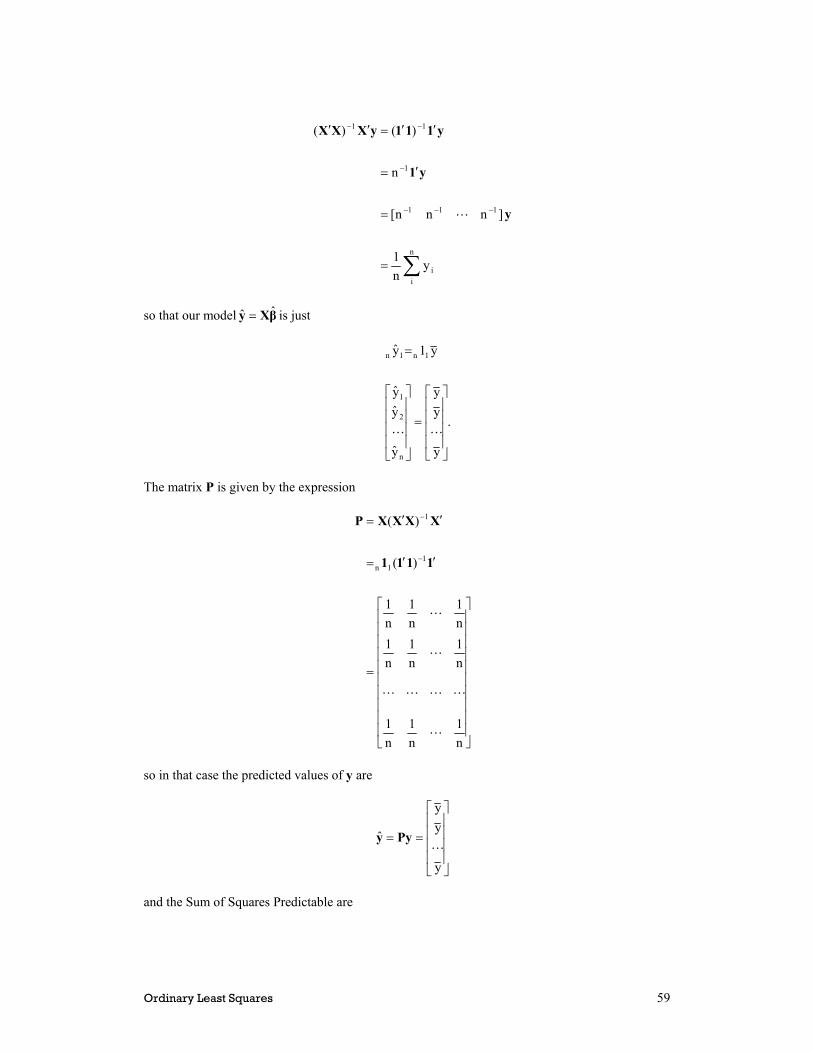
Ordinary Least Squares 59
∑=
=
′=
′′=′′
−−−
−
−−
n
ii
111
1
11
yn1
]nnn[
n
)()(
y
y1
y111yXXX
L
so that our model βXy ˆˆ = is just
.
y
yy
y
yy
y1y
n
2
1
1n1n
⎥⎥⎥⎥
⎦
⎤
⎢⎢⎢⎢
⎣
⎡
=
⎥⎥⎥⎥
⎦
⎤
⎢⎢⎢⎢
⎣
⎡
=
LL
The matrix P is given by the expression
⎥⎥⎥⎥⎥⎥⎥⎥⎥⎥
⎦
⎤
⎢⎢⎢⎢⎢⎢⎢⎢⎢⎢
⎣
⎡
=
′′=
′′=
−
−
n1
n1
n1
n1
n1
n1
n1
n1
n1
)(
)(
11n
1
L
LLLL
L
L
1111
XXXXP
so in that case the predicted values of y are
⎥⎥⎥⎥
⎦
⎤
⎢⎢⎢⎢
⎣
⎡
==
y
yy
ˆL
Pyy
and the Sum of Squares Predictable are

60 Chapter 5
∑=′= iedictedPr ySS yPyy . The M matrix also takes on a particular form in the intercept-only model.
⎥⎥⎥⎥⎥⎥⎥⎥⎥
⎦
⎤
⎢⎢⎢⎢⎢⎢⎢⎢⎢
⎣
⎡
−
⎥⎥⎥⎥⎥⎥⎥⎥
⎦
⎤
⎢⎢⎢⎢⎢⎢⎢⎢
⎣
⎡
=
−=′′−= −
n1
n1
n1
n1
n1
n1
n1
n1
n1
100
010
001
)( 1
L
LLLL
L
L
L
LLLL
L
L
PIXXXXIM
The M matrix transforms the observations in y into error, but in this case the “error” is equivalent to deviations from the mean (in other words di values):
⎥⎥⎥⎥⎥⎥
⎦
⎤
⎢⎢⎢⎢⎢⎢
⎣
⎡
−
−
−
==
yy
yy
yy
n
2
1
LMye .
The SSError is the quadratic form with M in the middle,
∑ ∑ ∑∑ ∑
∑
⎟⎟
⎠
⎞
⎜⎜
⎝
⎛−=−=
′=′−′=−′=
−=′=
,yn
yyyyy
)(
)yy(ySS
ii2
ii2i
iiError
yyy1yyyy1yy
Myy
which the reader will recognize as the scalar, the corrected sum of squares from Equation (2.11).
5.10 Response Surface Models While it is known as the linear model, one can fit more complicated curves than lines or planes. It is relatively straightforward to include quadratic or higher order polynomials in a regression model, merely by squaring or cubing one of the independent variables (it is wise to mean center first). For example, consider the model .xxxxy 4
22i32i2
21i11i0i β+β+β+β+β=

Ordinary Least Squares 61
The second and fourth independent variables are squared versions of the first and third. In order to demonstrate the wide variety of shapes we can model using polynomial equations, consider the figure below where β2 and β4 are either 0 or 1:
Or consider the following diagram in which the sign of β2 and β4 is either positive or minus:
02 =β 12 =β
04 =β
14 =β
1x2x
1x
1x 1x
2x
2x 2x
12 +=β 12 −=β
14 +=β
14 −=β
1x 1x
1x 1x
2x 2x
2x2x

62 Chapter 5
References Mosteller, Frederick and John W. Tukey (1977) Data Analysis and Regression. Reading, MA: Addison-Wesley.


64 Chapter 6
Chapter 6: Testing Linear Hypotheses Prerequisites: Chapter 5
6.1 The Distribution of the Regression Model Estimator According to Theorem (4.9), if we have a random vector a such that the variance of a is known, V(a) = C, lets say, then we can deduce the variance of any linear combination of a. Using the matrix D′ to create a set of linear combinations, we would have, in that case, V(D′a) = D′CD. We can use this key theorem to deduce the variance of ,β the vector of parameter estimates from the regression model, i. e. .)(ˆ 1 yXXXβ ′′= − Looking at the formula for ,β we see that we can apply the theorem with y playing the role of the random vector "a", and the premultiplying matrix (X′X)
-1X′ in its Oscar winning performance as
"D", creates k linear combinations from y. We know the variance of y, V(y) = V(Xβ + e) = V(e) = σ2I since y must have the same variance as e. This is so because adding a constant to a random vector does not change the variance of that vector, as is pointed out in Theorm (4.8). Given that, we can apply the theorem of Equation (4.9) such that
.)(
)()(
])[(])[()ˆ(V
12
112
121
−
−−
−−
′σ=
′′′σ=
′′′σ′′=
XX
XXIXXXX
XXXIXXXβ
(6.1)
To get to the last line we have used a variety of theorems from Chapter 1, including the associative property of scalar multiplication [Theorem (1.29)], and the fact that if A = A′, then A-1 = (A-1)′ which is presented in Equation (1.40). Now that we have a formula for the variance of ,β we are getting closer to being able to make inferences about β, the population value. Of course we are interested in the population, not just the particular sample that we happened to have observed. To make the leap from the sample to the population we need to talk about the probability distribution of .β Another very important theorem about linear combinations comes next. Lets assume we have a n by 1 random vector a and a constant vector b′. Then Central Limit →′ 1nn1 ab normality as (6.2) ∞→n . What this Central Limit theorem states is that a linear combination of a random vector tends towards normality as n, the number of elements in that vector increases towards infinity. In practice, n need only get to about 30 for this theorem to apply. What’s more, the theorem in no

Testing Linear Hypotheses 65
way depends on the distribution of the random vector a. To take one extreme example, a might contain a series of binary values; 0’s or 1’s; and the theorem would still apply! Turning back to the least squares estimator, ,β if we have a sample size more than 30, we can be fairly confident
that β will be normally distributed, even if the error vector e, and hence y, are not normally distributed. We can therefore conclude that ])(,[N~)(ˆ 121 −− ′σ′′= XXβyXXXβ . (6.3) It is now time to use a distribution that is applicable when the sample size is less than 30, the t-distribution (more information can be seen in Section 4.6). Consider the normally distributed scalar q, that is )]q(V),q(E[N~q . In that case the ratio
df~)q(V
)q(Eq t− . (6.4)
The subscript df on the t represents the degrees of freedom for the t-distribution, that is the effective number of observations used to estimate V(q) using ).q(V More specifically, in the case
of a particular element of ,β say ,ˆiβ we would have
kn
i
ii ~)ˆ(V
ˆ−
− tβ
ββ. (6.5)
We have already determined )ˆ(V iβ in Equation (6.1). In order to refer to this variance better, let us define D = (X′X)
-1 = dij.
The superscript notation, used with the element dij, is often used to describe the elements of the inverse of a matrix. Note that dii is the ith diagonal element of (X′X)
-1. Now we are in a position
to say that .d)ˆ(V ii2
i ⋅σ=β (6.6) All that remains to construct our t is to figure out how to estimate σ
2. This is done using
thatsokn
e
knSS
sˆ
n
i
2i
Error22
−=
−=≡σ
∑ (6.7)
ii2
i ds)ˆ(V ⋅=β . (6.8) Instead of using Equation (6.7) to calculate s
2, we can also use the covariance approach (see
Equation (5.25):

66 Chapter 6
xyxxyxyy2 ss sSs−= .
In addition to being the empirical estimate of the variance of the ei, s
2 is also the variance of y | X,
that is, y conditional on the observed values of X.
6.2 A 1 - α Confidence Interval
Finally, we are ready to make statements about the population values of .β There are two broad ways of doing this. The first, which will be given immediately below, is called a confidence interval. The second will be covered in the next section and involves all-or-nothing decisions about hypotheses. A 1 - α confidence interval for the element iβ is given by ii2
kn,2/i dstˆ−α±β (6.9)
which means that
,1dstˆdstˆPr ii2kn,2/ii
ii2kn,2/i α−=⎥⎦
⎤⎢⎣⎡ +β≤β≤−β −α−α (6.10)
where tα/2, n-k is the tabled t-statistic with n - k degrees of freedom such that Pr(t ≥ tα/2) = α/2. The upshot is that, with a probability of 1 - α, we can capture the population value of a parameter of interest between the minus and plus values of the confidence interval. The benefit of this procedure is that we can pick α a priori according to our tolerance for risk. Of course picking a smaller value of α (which reduces the risk of missing the target, βi) implies a larger value of t in the formula which in turn expands the distance between the left and right end points of the interval. Despite the elegance of confidence intervals, marketers do not usually use them. Marketing theory rarely provides us with enough information to motivate us to look at particular values of the βi. At best, it seems our theories may be capable of letting us intuit the sign of βi. We can then decide if we were right about our intuition using a yes or no decision, a procedure that we will now address.
6.3 Statistical Hypothesis Testing Questions about marketing theory, as well as practitioner issues, that are explored using samples, are often solved through the use of statistical hypothesis testing. For example, we might be interested in testing the hypothesis H0: βi = c where c is a constant suggested by some a priori theory. It is important to note that the entire logical edifice that we are going to build in this section is based on the presumption that this hypothesis was indeed specified a priori, that is to say, specified before the researcher has looked at the data. In that case we need to create a mutually exclusive hypothesis that logically includes all possible alternative hypotheses. Thus, between the two hypotheses we have exhaustively described the outcome space; all outcome possibilities have been covered. Given the hypothesis above, the alternative must be HA: βi ≠ c.

Testing Linear Hypotheses 67
We need to acknowledge that the two hypotheses are not symmetric. For one thing, Ho is specific while HA is more general. You will note that H0 is always associated with an equality. For another thing, the two sorts of mistakes that we can make, namely, believing in H0 while HA is actually true; vs. believing in HA while H0 is true; are not symmetric. Part of the definition of H0 is that it is the hypothesis that we will believe in by default, unless the evidence is overwhelmingly against it. In some cases we can define H0 for its “safety.” That is, if we have two mutually exclusive hypotheses, and falsely believing in one of them, even though the other is true, is not so damaging or expensive, we would want to pick that one as H0. We now need to summarize the evidence for and against H0 and HA. Here is where the t statistic comes in. We will assume that H0 is true. In that case,
knii2
i
i
ii ~ds
cˆ
)ˆ(V
ˆˆ
−−
=−
= tt β
β
ββ . (6.11)
We can now evaluate the probability of this evidence assuming that H0 is true by simply looking up the probability of t based on the t-distribution. Specifically, we reject H0 if ,t| ˆ| k-n /2,t α> (6.12) where tα/2, n-k is the tabled t-statistic with n - k degrees of freedom such that Pr(t ≥ tα/2) = α/2. The value α can once again be chosen a priori according to one’s tolerance for the risk of falsely rejecting H0, an error often referred to as being of Type I. The value α is divided in two simply because HA has two tails, that is to say, it is the nature of H0 that it can be wrong in either of two directions. In some sorts of hypotheses we do not need to divide α by two. If we have H0: βi ≥ c, which implies an alternative of HA: βi < c, there is only one direction or tail in which H0 can be wrong. In that case we reject H0 if k-n ,tt α> . (6.13) The inequality obviously reverses direction if H0 involves a “≤”. Note that one way or the other, H0 allows the possibility of an equality. The logic of hypothesis testing is based on H0. It is the only hypothesis being tested. Rejecting H0 we learn something, we can make a statement about the population. Otherwise we have simply failed to reject it and we must leave it at that. Generally speaking, those writing articles for marketing journals tend to automatically pick α = .05. It’s a social convention, but the arbitrariness of “.05” should not obscure the value we get out of picking some value a priori. In some practitioner applications the two possible types of errors can be assigned a monetary value and the choice of α can be optimized.
6.4 More Complex Hypotheses and the t-statistic It is possible to look at more complex questions, for example is β1 = β2? We will write the question as a linear combination of the β vector:

68 Chapter 6
[ ] .000110:H
c:H
*k
3
2
1
0
0
0
=
⎥⎥⎥⎥⎥⎥⎥⎥
⎦
⎤
⎢⎢⎢⎢⎢⎢⎢⎢
⎣
⎡
β
ββββ
−
=′
L
L
βa
We can create a t-test using the same technique as before as long as we can figure out the denominator of the t. The theorem we discussed at the beginning of the chapter, Theorem (4.9) which lets us derive the variance of a linear combination of a random variable can guide us once again:
.)(
)ˆ(V)ˆ(V
12 aXXa
aβaβa
−′′σ=
′=′
(6.14)
By substituting the empirical estimate, s2 for the population value σ2, we get the formula for the t that lets us test the linear hypothesis H0 against the alternative, HA: a′β ≠ c
.)(s
cˆˆ
12 aXXa
βa−′′
−′=t (6.15)
As before, we would reject H0 if kn,2/
ˆ| −α> t|t . We might note that the basic t-test discussed in the previous section to test H0: βi = 0 is a special case of this procedure with [ ].001000 LL=′a In general, if you can quantify a hypothesis as a single linear combination, so that the right hand side is a scalar and there is just one equal sign, you can test it with a t-test. But we can test even more complex hypotheses than these, and that is the subject of the next section, Section 6.5.
6.5 Multiple Degree of Freedom Hypotheses We will now look at more complicated hypotheses that require more than a single linear combination. Where before our hypothesis was represented in a′, now we will have a series of hypotheses in the q rows of the hypothesis matrix A. We can simultaneously test all q of these hypotheses,

Testing Linear Hypotheses 69
⎥⎥⎥⎥⎥
⎦
⎤
⎢⎢⎢⎢⎢
⎣
⎡
=
⎥⎥⎥⎥⎥
⎦
⎤
⎢⎢⎢⎢⎢
⎣
⎡
′
′′
=
q
2
1
.q
.2
.1
0
1q0
c
cc
:H
:H
LLβ
a
aa
cAβ
(6.16)
As an example, suppose we wanted to simultaneously test that β2 = 0, and that β3 = 0, or more concisely, that β2 = β3 = 0. We can use an A matrix as below,
⎥⎥⎦
⎤
⎢⎢⎣
⎡=
⎥⎥⎥⎥⎥⎥
⎦
⎤
⎢⎢⎢⎢⎢⎢
⎣
⎡
⎥⎥⎦
⎤
⎢⎢⎣
⎡
0
0
1000
0100:H
3
2
1
0
0
β
β
β
β
.
The flexibility of linear hypotheses cannot be exaggerated. Suppose we want to test that a set of β coefficients are equal; β1 = β2 = β3. That can be coded into the A matrix as
⎥⎥⎦
⎤
⎢⎢⎣
⎡=
⎥⎥⎥⎥⎥⎥
⎦
⎤
⎢⎢⎢⎢⎢⎢
⎣
⎡
⎥⎥⎦
⎤
⎢⎢⎣
⎡
−
−
0
0
1010
0110:H
3
2
1
0
0
β
β
β
β
.
To test these sorts of hypotheses, we will be using the F distribution, which is more general than the t. In fact, an F with one degree of freedom in the numerator is equivalent to a t squared. (This is briefly discussed in Section 4.7.) An F is a ratio of variances. Under the null hypothesis, both the numerator and the denominator variances measure the same thing so that the average F is one. In the case of the linear hypothesis H0: Aβ = c, the numerator is the variance attributable to the hypothesis. In this context the variance is called a mean square - in other words it is an average sum of squares. To calculate the sum of squares that will be used for this mean square, we have: [ ] ).ˆ()()ˆ(SS
11H cβAAXXAcβA −′′′−=
−− (6.17) Since β is a column vector, and this is a single quadratic form, SSH is a scalar. For this to work the A matrix, which is q by k, has to have q independent rows, and certainly q must be less than or equal to k. Otherwise, the matrix within the brackets will not be capable of being inverted. Given that A has q independent rows, we can set up the ratio
kn,qError
H F~kn/SS
q/SS−−
(6.18)
which can be used to test the hypotheses embodied in the A matrix.

70 Chapter 6
Typically a variance is an average sum of squares divided by "n - 1" which represents the degrees of freedom of that variance. In this case, in the numerator, the average is being taken over the q rows of A. In other words, the number of observations - the degrees of freedom - is q. The denominator, which the reader should recognize as the variance of the ei, called s2, has n – k degrees of freedom. (We remind you that k represents the number of other parameters estimated in the regression model. We have already estimated values for theβ vector.) leaving n – k observations for estimating s2.
6.6 An Alternative Method to Estimate Sums of Squares for an Hypothesis Let us return to one of the multiple degrees of freedom hypotheses we looked at above,
⎥⎥⎦
⎤
⎢⎢⎣
⎡=
⎥⎥⎥⎥⎥⎥
⎦
⎤
⎢⎢⎢⎢⎢⎢
⎣
⎡
⎥⎥⎦
⎤
⎢⎢⎣
⎡
0
0
1000
0100:H
3
2
1
0
0
β
β
β
β
.
We are hypothesizing that two of the betas are zero, which implies that the independent variables associated with them vanish from the regression equation, being multiplied by zeroes. Lets call the model that is missing x2 and x3 the “Restricted Model.” We could calculate the Sum of Squares Error for this model and compare it to the usual Sum of Squares Error. The difference, illustrated below, provides an alternative way of assessing the hypothesis: SSH = SSError (Restricted Model) – SSError (Full Model) Since the restricted model has fewer variables, it’s SSError cannot be less than the SSError for the full model, thus SSH must be positive; it is after all a sum of squares, so it had better be positive!
6.7 The Impact of All the Independent Variables We often wonder if any of our independent variables are doing anything at all, if between them, we are achieving any prediction or explanation of the dependent variable. We can express this question using the hypothesis 0:H *k210 ==== βββ L . (6.19) The only β value missing from the hypothesis is β0, which is usually not of any theoretical importance. The hypothesis asks if we can get any additional prediction, above and beyond the mean which is represented by β0. The F given below,
kn/)Full(SS
*k/)Full(SS)tostricted(ReSSF
Error
Error0Error
−−β
= (6.20)
can be compared to the tabled value of Fα, k*, n-k. We can also summarize the predictive power of all the independent variables (except x0) using Big R Squared, also known as the squared multiple correlation or SMC, shown below:

Testing Linear Hypotheses 71
)Full(SS
)Full(SS)tostricted(ReSSR
Error
Error0Error2 −β= . (6.21)
Now we will look at some alternative formulae for these Sums of Squares for Error. For example,
.e)yy()Full(SS
and)yy()tostricted(ReSS
i
2i
i
2iiError
i
2i0Error
∑∑
∑
=−=
−=β
Using these terms, we can say that ∑ ∑∑ −+−=−
i i
2ii
2i
i
2i )yy()yy()yy( or in words (6.22)
Corrected SS = SS Due to Real Independent Variables + SS Error. We can prove this by looking at the definition of SSError:
.ˆˆ
ˆˆ
yyyy'
βXXβyy'ee'
′−=
′−=
By rearranging we have
∑∑∑ −+−=−
+−′=−
+′=
i
2ii
i
2i
i
2i )yy()yy()yy(
ynˆˆyn
ˆˆ
ee'yyyy'
ee'yyyy'
This allows us to restate R2 as

72 Chapter 6
.)yy(
)yy(
)yy(
e1
)yy(
e)yy(R
i
2i
2
ii
i
2i
i
2i
i
2i
i i
2i
2i
2
∑∑
∑∑
∑∑ ∑
−
−=
−−=
−
−−=
In summary, R2 summarizes the proportion of the corrected Sum of Squares, and of the variance, of y which is explained by each of the independent variables, x1, x2, …, xk* . The hypothesis H0: ρ
2 = 0 (note that rho, ρ, is the Greek equivalent to r) is equivalent to the hypothesis that β1 = β2 = ··· = βk* = 0.
6.8 Generalized Least Squares There are many circumstances where we cannot believe the Gauss-Markov assumption. Suppose for example that the variance of the errors is not σ2I but rather follows some more general form, σ2V where V is a symmetric matrix. If V is diagonal, the technique of this section is called weighted least squares or WLS. If V is symmetric, it is called generalized least squares, or GLS. Of course, if the elements of V are not known, we would run out of degrees of freedom trying to estimate the elements of both β and V. But in many cases, we have an a priori notion of what V should look like. For example, we can take advantage of the fact that the variance of the population proportion π is known and is in fact equal to π(1 - π)/n. If our dependent variable consists of a set of proportions, we can modify the Gauss-Markov assumption accordingly and perform weighted least squares. Instead of minimizing e′e, we minimize f = e′V-1e, (6.23) where the diagonal elements of V consist of the values π(1 - π)/n for appropriate to each observed proportion. We can look at this technique as minimizing the sum of squares for a set of transformed errors. The transformed errors have constant variance and therefore are appropriate for the Gauss-Markov assumption. Our estimate of the unknowns becomes yVXXVXβ 111 ][ˆ −−− ′′= . (6.24) We can estimate σ
2 using
kn
SSs Error2
−=
where

Testing Linear Hypotheses 73
)ˆ()ˆ(SS 1Error βXyVβXy −′−= − .
We can construct t-statistics that allow us to test hypotheses of the form H0: βi = 0 using the ith diagonal element of s
2(X′V
-1X)
-1 in the denominator to create a t. One can also test
one degree of freedom hypotheses such as a′β = c using
aXVXa
βa112 )(s
cˆˆ−−′′
−′=t
and for more complex hypotheses of the form H0: Aβ - c = 0 we use )ˆ(])([)ˆ(SS 111
H cβAAXVXAcβA −′′−= −−− to construct an F ratio numerator, with s
2 in the denominator.
This result is discussed in more detail in Section 17.4.
6.9 Symmetric and Idempotent Matrices in Least Squares Define P = X(X′X)
-1X′ and define M = I – P, i. e. I - X(X′X)
-1X′. Now recall Equation (5.21) for
the SSError:
.
][
)( 1
Myy
yPIy
PyyIyy
yXXXXyyyee
′=
−′=
′−′=
′′′−′=′ −
(6.25)
What this tells us is that the SSError is a quadratic form, with the matrix M in the middle. The SSPredicted is a quadratic form also, with P in the middle,

74 Chapter 6
PyyyXXXXy ′=′′′ −1)( and as we might imagine, the raw total sum of squares of the dependent variable is a quadratic form, with the identity matrix in the middle: y′y = y′Iy. So now we have some relationships among SSTotal, SSPredictable and SSError, namely SSTotal = SSPredictable + SSError y′Iy = y′Py + y′My and (6.26) I = P + M. (6.27) At this point we might note that the Identity matrix I is of full rank (Section 3.7), that is to say, |I| ≠ 0, but both P and M are not with P having rank k and M rank n - k, the same as their degrees of freedom. What’s more, P transforms y into ,y and M transforms y into e as can be seen below:
Py
yXXXX
yXXXXβXy
=
′′=
′′==
−
−
])([
])[(ˆˆ
1
1
(6.28)
and
My
yXXXXyβXye
=
′′−=−= − ])[(ˆ 1
(6.29)
So that we can think of P as the prediction transform or prediction operator, that is, a set of linear combinations that transform y into ,y while M is the error transform or error operator that transforms y into e. These matrices have some even more unusual properties, namely: Symmetry M = M′, P = P′ (6.30) Idempotency MM = M, PP = P, (6.31) and also,

Testing Linear Hypotheses 75
.nn
n1nnn1
n1nnn1
0PM
0P1
0M1
=
′=′
′=′
and (6.32)
More details of on the importance of M and P can be found in Section 4.5. In summary, since y′y = y′Iy = y′Py + y′My, we can show that these sums of squares components are distributed as Chi Square.
References Graybill, Franklin (1976) Theory and Application of the Linear Model. Belmont, CA: Wadsworth. Sawyer, Alan G. and J. Paul Peter (1983) "The Significance of Statistical Significance Tests in Marketing Research," Journal of Marketing Research, 20 (May), 122-33.

76 Chapter 7
Chapter 7: The Analysis of Variance Prerequisites: Chapter 6
7.1 History and Overview of ANOVA The analysis of variance is often used to test for group differences – very frequently different groups of consumers who have been exposed to various treatments. The word treatment obviously makes reference to the early days of the technique from biology early in the 20th century. In the context of marketing, a classic and simple example might involve different ads viewed by the different groups. Of course ANOVA is applicable to analyses of pre-existing groups as well. The historical roots of ANOVA go back long before the existence of computers and before text writers acknowledged that the regression technique of Chapters 5 and 6, and ANOVA, are basically one and the same. Of course, today, all the major statistical packages compute ANOVA as a special case of regression. And understanding ANOVA in this way will add to the student’s intuition about what is going on. However, there are at least two different ways of notating ANOVA: an older method that relied on calculating machines and that uses multiple subscripts on the dependent variable, and the newer way that is optimized for computer calculation that uses one subscript as the observations are stacked in the vector y. In what follows we will offer a brief review of the older notation while demonstrating how it relates to the newer regression-centric view. In what follows we will also assume that we have some sort of qualitative variable that divides the population into A groups indexed by a = 1, 2, ···, A. The observations from these groups might be represented as yia, that is, observation i from group a. A pictorial representation of the situation might look like the following
You can see that the second subscript is indexing group membership while the first keeps track of the individual within that group. Further, in group a, the sample size is na with that observation being the last case in group a. This is known as a one-way analysis of variance, since there is but a single qualitative variable that identifies group membership. The traditional test of the null hypothesis involves the population means and whether they are all equal, viz. .:H A210 μ==μ=μ L (7.1) In general, we would estimate the population mean μa using the sample mean .yˆ a.a =μ The subscript for the ,y a. the “·a” is taken from Equation (1.2) and is now holding the place of the eliminated first subscript in the data, the one that tracks the individual observation. Remaining with the older tradition, we say that our model is
1n
21
11
1y
yy
L
2n
22
12
2y
yy
L
An
A2
A1
Ay
yy
L···
Group 1 Group 2 Group A

The Analysis of Variance 77
,ey iaaia +α+μ= (7.2) with μ being the overall mean, and the αa quantifying the impact of group membership. The eia represent error in the model, and in this case we can say that it is an error particular to group a. The problem is that we have exactly A unique groups – and A values of a.y in our data – but we have A + 1 parameters. That is, there are A αa plus one μ. We need to restrict the αa in some way. This problem is related to the idea that in the statement of the null hypothesis in Equation (7.1), there are A – 1 equal signs, not A of them. We are not interested in the levels of the group means per se, but in the differences between the levels of the group means. It turns out there are at least three popular ways to parameterize this model (of course there are an infinite number of ways to do it in general). The first one, covered next, is called effect coding.
7.2 Effect Coding One thing we can do is impose the restriction
,0A
aa =α∑ (7.3)
for example by setting .1A21A −α−−α−α−=α L The αa represent the effect of being in group a: ⋅⋅⋅ −=α yy aa (7.4) where ⋅⋅y is clearly equivalent to μ. At this time, let us think about how this model, as parameterized above, relates to regression. In the regression model y = Xβ + e, the qualitative independent variable must be represented somehow using the columns of X. The αa must end up in the β matrix, or at least A – 1 of them must do so. We can, as we saw above, solve for the last one by subtraction. To illustrate how to implement effect coding lets say we have A = 4 groups. We do not have to show all of the subjects in all of the groups since the model for all of the subjects within each group must be identical. It will suffice to show the model for the i-th subject in each group. To the extent that any two members of the same group do not have the same score, this contributes to the error term. Now, our model will be
.
1111100101010011
yyyy
3
2
1
0
4i
3i
2i
1i
⎥⎥⎥⎥
⎦
⎤
⎢⎢⎢⎢
⎣
⎡
ββββ
⎥⎥⎥⎥
⎦
⎤
⎢⎢⎢⎢
⎣
⎡
−−−
=
⎥⎥⎥⎥
⎦
⎤
⎢⎢⎢⎢
⎣
⎡
(7.5)
It is worth contemplating the columns of X for a bit. The first one is clearly just the classic y-intercept, just as it has always been in Chapters 5 and 6. The last three columns code for group membership. The first vector coding for groups has a plus one for group 1 and a -1 for the last group. Zeroes appear in every other row of that column. The second group membership vector repeats the pattern but the plus one goes against group two. Finally, the last vector has a one in the next to last position, a minus one in the last position and zeroes elsewhere. To summarize, each column x·j (j = 1, 2, ···, A-1) gets a 1 for group j, a negative 1 for group A, and everything else is null. Writing out the model in scalar terms reveals

78 Chapter 7
.y
andy
,y
,y
32104i
303i
202i
101i
β−β−β−β=
β+β=
β+β=
β+β=
The null hypothesis 0:H 3210 =β=β=β is mathematically equivalent to .:H 43210 μ=μ=μ=μ While the proof of this equivalence will be left to the interested reader, one can see that both statements have three equalities. Using the methods of Chapter 6, we can set up the hypothesis matrix
⎥⎥⎥
⎦
⎤
⎢⎢⎢
⎣
⎡=
100001000010
A ,
which having three rows, provides an overall three degree of freedom test of no mean differences. Individual one degree of freedom tests for any of the βj may or may not be of interest. H0: βj = 0 is equivalent to H0: μj - μ = 0, that is, that there is no significant effect of being in group j.
7.3 Dummy Coding In our model, ,ey iaaia +α+μ= (7.6) there are multiple ways to resolve the ambiguities and identify the model. We now cover the second one in which we impose the restriction αA = 0 (7.7) which then implies that Ay ⋅=μ and Aaa yy ⋅⋅ −=α . The coding for the design matrix looks like this:

The Analysis of Variance 79
.
0001
1001
0101
0011
y
y
y
y
3
2
1
0
4i
3i
2i
1i
⎥⎥⎥⎥⎥⎥
⎦
⎤
⎢⎢⎢⎢⎢⎢
⎣
⎡
β
β
β
β
⎥⎥⎥⎥⎥⎥
⎦
⎤
⎢⎢⎢⎢⎢⎢
⎣
⎡
=
⎥⎥⎥⎥⎥⎥
⎦
⎤
⎢⎢⎢⎢⎢⎢
⎣
⎡
The columns of X are often called dummy variables since each value is either a '1' or a '0'. This means that
.y
andy
,y
,y
04i
303i
202i
101i
β=
β+β=
β+β=
β+β=
You can see that column x·j gets a '1' for group j, j = 1, 2, ···, A - 1. Everything else gets a '0'. As before, H0: β1 = β2 = β3 = 0 tests H0: μ1 = μ2 = μ3 = μ4, and we can construct the A hypothesis matrix as above in equation (7.5). Test of individual βj values are probably not interesting since H0: βj = 0 is equivalent to H0: μj - μA = 0. However, this might be interesting if the last group, group A, is some sort of control group and the researcher wants to compare some of the other groups to the last one. Note that both systems of coding lead to the same 3 degree of freedom F with the same value. What varies is how these three degrees of freedom are partitioned. And now we look at the final method of partitioning group effects, orthogonal coding.
7.4 Orthogonal Coding In the previous two methods of coding, effect and dummy coding, the columns of X are correlated which is to say they are not orthogonal, a concept defined in Equation (1.17). In this section we describe a method of coding the design matrix in such a way that X′X is a diagonal matrix. Of course this means that the columns of X are all mutually orthogonal, meaning that the inner product is zero. There are very many ways of doing this, but here is one simple scheme that can be used to create orthogonal columns in X:
⎥⎥⎥⎥
⎦
⎤
⎢⎢⎢⎢
⎣
⎡
−−−−−−
=
3001120111111111
X .
The pattern should be clear - column j has j '-1's and one 'j'. Here we see that H0: β1 = 0 is equivalent to H0: μ1 = μ2; H0: β2 = 0 is equivalent to H0: ;2)( 321 μ=μ+μ and H0: β3 = 0 is equivalent to H0: .3)( 4321 μ=μ+μ+μ

80 Chapter 7
One can modify the scheme to test certain planned comparisons of interest. Suppose we had planned a priori to test H0: μ2 = μ3. We can set the second column of X to embody this comparison:
⎥⎥⎥⎥
⎦
⎤
⎢⎢⎢⎢
⎣
⎡
−−−−−−
=
3001111111111201
X
which the reader can see as effectively identical to the example immediately above, but changing the order of the rows. At this point we need only test the hypothesis that β1 = 0.
Now suppose we wish to compare groups 1 and 2 against 3 and 4, i.e. that .22
4321 μ+μ=
μ+μ
We can use X as below:
⎥⎥⎥⎥
⎦
⎤
⎢⎢⎢⎢
⎣
⎡
−−−−−−
=
1111111111111111
X .
Here we can test our hypothesis using β1. The pattern of signs in the second column of X (the column pertaining to β1) allows you to interpret the sign of β1. If β1 is positive it means that the first two means are greater than the second two. Note that in all the cases we have discussed in this section, we have orthogonal columns of X. This leads to an ease of interpretation of the β's.
7.5 Interactive Effects In many cases in marketing the impact of one independent variable depends on the specific values of another independent variable. For example, we might find that as price increases, consumer purchase intention is reduced, except when there is the presence of advertising. This is illustrated in the hypothetical interaction plot below:

The Analysis of Variance 81
An interaction limits our ability to generalize. If you were to summarize the impact of Price on Purchase Intent, you would have to take into account the value of the other independent variable, Advertising. By the same token, if you were to try to describe what effect Advertising has on Intent, you would have to pull Price into the explanation. An interaction is characterized by non-parallel lines in an interaction plot, as is shown above. Interactions of many forms are possible, but the linear model can subsume any interactive effect by including columns in the design matrix X which consist of the products of other columns of X. To see this, look at the design matrix pictured below:
The subscripts on the dependent variable values run from L to M to H (low, medium and high) to index the level of the price variable and from A to N to indicate advertising vs. no-advertising. Column 0 of the X matrix codes for the usual intercept term. Column 1 uses orthogonal coding to register the difference in the level of advertising, while columns 2 and 3 use orthogonal coding to track the 3 levels of Price. With three levels, Price has 2 degrees of freedom, which is to say, 2 columns in X. The fourth column of X is the product of columns 1 and 2, while the fifth column is the product of columns 1 and 3. The interaction between Price and Advertising also has 2 degrees of freedom. The reader might notice that all six columns of X are mutually orthogonal.
Price
Low Med Hi
Purchase Intent
No Ad
Advertising
⎥⎥⎥⎥⎥⎥⎥⎥
⎦
⎤
⎢⎢⎢⎢⎢⎢⎢⎢
⎣
⎡
ββββββ
⎥⎥⎥⎥⎥⎥⎥⎥
⎦
⎤
⎢⎢⎢⎢⎢⎢⎢⎢
⎣
⎡
−−−−
−−−−−−−
−−−
=
⎥⎥⎥⎥⎥⎥⎥⎥
⎦
⎤
⎢⎢⎢⎢⎢⎢⎢⎢
⎣
⎡
5
4
3
2
1
0
iLN
iLA
iMN
iMA
iHN
iHA
202011202011111111111111111111111111
yyyyyy
Ad: A vs. N Price: H, M, L
214 xxx ⋅⋅⋅ =
315 xxx ⋅⋅⋅ =

82 Chapter 7
7.6 Quantitative Independent Variables We can actually use the linear regression model to fit a non-linear model. Almost any quantitative function can be approximated by a polynomial of sufficiently high order. Consider the model below: im
mi3
3i2
2i1i0i exxxxy ++++++= βββββ L (7.8)
To make this model work, one should first deviate the xi from the mean to avoid problems of high correlation between the columns of the X matrix. With a relatively small number of levels of the quantitative independent variable, you can use the method of orthogonal polynomials instead. Any function can be represented as a polynomial with sufficiently high order. A curve with one elbow can be expressed as a quadratic function, one with two elbows can be imitated with a cubic function, and so on from quartic, quintic, etc. For example, we might be concerned with the shape of the relationship between the length of an ad viewed by subjects, and their attitude towards that ad. Imagine that one group saw a 1 minute ad, another a 2 minute ad, and there were also 3 and 4 minute groups. Presuming that the ad is affective, the relationship could take on a variety of forms, such as those pictured below:
On the far right is pictured a very simple linear assumption, in the middle a curve with one elbow, and on the left a more complex curve requiring a cubic component. We might construct the design matrix as below using
⎥⎥⎥⎥
⎦
⎤
⎢⎢⎢⎢
⎣
⎡
=
6416412793184211111
X
but it would be smarter to use a columns that were not so highly correlated. As mentioned above, if you column-center the linear component and then use it as a basis for creating the other columns, this will help. You can also use orthogonal polynomials (see the tables in Bock 1975 for example):
.
1131311131111131
⎥⎥⎥⎥
⎦
⎤
⎢⎢⎢⎢
⎣
⎡
−−
−−−−
=X
Length of Ad
Attitude Attitude Attitude
Length of Ad Length of Ad

The Analysis of Variance 83
One could then test the necessity of the cubic term, assuming a linear and quadratic component using a t-test. If that proves non-significant, one could go on and test the necessity of the quadratic term.
7.7 Repeated Measures Analysis of Variance A special case of the analysis of variance occurs when we have a set of commensurate variables, or commensurate measures. The expression implies that the same scale is repeatedly applied on several measurement occasions. For example, perhaps consumers are asked to rate four brands using a particular measure. Repeated measures are multivariate in nature, meaning that there is more than one dependent variable. In the example with four brands, there would be four dependent variables. We define yij as the measurement on person i, on measure j, with i = 1, 2, ···, n and j = 1, 2, ···, p. There are two ways to treat such data. We can place all of the measurements in a matrix, Y, with a row for each subject and a column for each measure. This is the multivariate approach, a topic covered in Chapter 8. For now, we will note that with four brands, and p = 4, the hypothesis that the means of the four brands are equal, i.e. that the columns of Y have equal means, is equivalent to the hypothesis that the three columns of Y~ below have means of zero. The matrix Y~ is given by Y~ = YM (7.9)
.
300120111111
~
⎥⎥⎥⎥
⎦
⎤
⎢⎢⎢⎢
⎣
⎡
−−
−= YY (7.10)
The hypothesis matrix M, when used to postmultipy the original data matrix Y, transforms the columns of Y into new columns in .~Y The first new column consists of the difference between the old columns 1 and 2. The second new column in Y~ is the difference between the combination of columns 1 and 2 and column 3, and so forth. The univariate approach stacks all of the data in a single vector, called y, in such a way that each subject's data appears contiguously, i.e. ]yyyyyyyyy[ np2n1np22221p11211 LLLL=′y We can then say that
⎥⎥⎥⎥⎥⎥
⎦
⎤
⎢⎢⎢⎢⎢⎢
⎣
⎡
=
Σ00
0Σ0
00Σ
y
L
LLLL
L
L
)(V (7.11)
where each Σ and each 0 is a p by p matrix. There are n of them, so that the entire variance matrix of y is np by np. That the covariance matrix of each subject, Σ, is homogeneous or identical from

84 Chapter 7
one subject to the next, is only an assumption, analogous to the assumption of homogeneity of variance of the scalar σ
2 in regular ANOVA.
To use the univariate approach to repeated measures, the variance of the transformed measures must be homogeneous and independent, that is IΣMM 2σ=′ (7.12) where the M matrix is the hypothesis matrix from above, Σ is the p by p (in our example with four brands, four by four) covariance matrix of the original measures, and σ2I is a scalar matrix with identical values along the diagonal (three identical values in our example with four brands). Often this assumption is called sphericity. If this assumption is met, we can use univariate analysis of variance as will now be described using an example.
7.8 A Classic Repeated Measures Example Imagine that we have three factors including one between subjects variable that divides subjects into two groups, a within-subjects factor with three levels and a within subjects variable that has four levels. All told our design is a 2 × 3 × 4 design, with the three factors named A, B and C. We can further imagine that we have 10 subjects, and since each subject is measured 12 times (since the repeated measures part of the design, B x C, involves 12 measures), we have a total of 120 data points. The results of such an ANOVA are typically described in an ANOVA table. A table for this design could look like this;
Source of Variance df Error Term A 1 S(A) S(A) 8 - Between-Subjects Total 9 - B C BC AB AC ABC S(A) · B S(A) · C SA(A) · BC
2 3 6 2 3 6 16 24 48
S(A) · B S(A) · C S(A) · BC S(A) · B S(A) · C S(A) · BC - - -
Within-Subjects Total 110 - TOTAL 119 -
The notation in the table bears some explanation. S(A) is used to represent Subjects within levels of the A factor. In other words, subjects are nested within groups since the same subject does not appear in more than one group. In contrast, Subjects are crossed with the two repeated measures: B and C. In addition, the factor Subjects is a random effect. This means that the "levels" of Subjects were randomly sampled from some larger population to which we would like to generalize our results. In contrast, A, B and C are fixed effects whose levels are chosen for their inherent interest to the experimenter, and hopefully for that person, the reviewers. You might note that the correct error term for the grouping factor is Subjects within groups. The correct error term for any repeated measures factor is that factor by Subjects interaction. In general terms, consider a purely within-subject effect, w, a purely between-subject effect, b, and

The Analysis of Variance 85
their interaction, wb. Either w or b may be main effects, interactions, or special contrasts. The error term for b is Subjects nested in groups. The error term for w is Subjects · w and the error term for wb is also Subjects · w. Homogeneity of Subject variance within groups is a needed assumption, as is the spherecity of transformed measures as described above in Equation (7.12).
References R. Darrell Bock (1975) Multivariate Statistical Methods in Behavioral Research. New York: McGraw-Hill. Box, George E. P., William G. Hunter, J. Stuart Hunter (1978) Statistics for Experimenters. New York: Wiley. Glantz, Stanton A. and Bryan K. Slinker (1990) Primer of Applied Regression and Analysis of Variance. New York: McGraw-Hill. Kirk, Roger E. (1982) Experimental Design. Second Edition. Pacific Grove, CA: Brooks/Cole. Mendenhall, William (1968) The Design and Analysis of Experiments. Belmont,CA: Duxbury.

86 Chapter 8
Chapter 8: The Multivariate General Linear Model Requirements: Sections 3.4, 3.5 - 3.8, 4.3 Chapter 7
8.1 Introduction The main difference between this chapter and the chapters on the General Linear Model; 5, 6 and 7; lies in the fact that here we are going to explicitly consider multiple dependent variables. Multiple dependent variables are to some extent discussed in Chapter 7 in the context of the analysis of variance. In that chapter, however, we made an assumption about the error distribution which allowed us to treat the problem as essentially univariate [see Equation (7.12)]. In this chapter, we will be dealing with multiple dependent variables in the most general way possible, namely the multivariate general linear model. Before we begin, it will be necessary to review some of the fundamentals of hypothesis testing, and then after, to introduce some mathematical details of use in this area.
8.2 Testing Multiple Hypotheses In Chapter 6, we covered two different approaches to testing hypotheses about the coefficients of the linear model. In Equation (6.15) we had
aXXa
βa12 )(s
cˆ−′′
−′=t
that allows us to test one degree of freedom questions of the form a'β = c, while in Equation (6.18) we have the test statistic
kn/SS
q/SSFError
H
−=
that allows us to test multiple degree of freedom questions Aβ = C. In the former case we have n - k degrees of freedom, and in the latter, q and n - k degrees of freedom. In that chapter we made the implicit assumption that these tests had been planned a priori, and that they were relatively few in number. In the case of multiple dependent variables, this second assumption becomes far less tenable. We begin by discussing a way to test hypotheses even when there are a large number of them. We then discuss the case where this large number of hypotheses might even be post hoc. 8.3 The Dunn-Bonferroni Correction What can we do if we wish to test a large number of hypotheses, say, H1, H2, ···, Hr? For any particular hypothesis, we can limit the probability that we reject H0 when it was indeed true of the population, that is we can limit Pr(Type I Error on Hi) = αi. But what is the probability of at least one Type I error in a sequence of r hypotheses? To delve into this question it will be useful to utilize the notation of Set Theory, where ∪ symbolizes union and ∩ symbolizes intersection. The probability of at least one Type I error is

The Multivariate General Linear Model 87
α* = Pr(Type I error on H1 ∪ Type I Error on H2 ∪ ··· ∪ Type I Error on Hr ). (8.1) We can think of α* as the overall α rate, the probability of at least on Type I Error. Define Ei as a Type I error event for Hi. From probability theory, with r = 2 hypotheses, lets say, the situation is illustrated below:
Two parts of the outcome space are shaded, the two parts that correspond to E1 (a Type I Error on H1) and E2 (a similar result on H2). There is some overlap, namely the part of the space comprising the intersection of E1 and E2. It can be shown that Pr(E1 ∪ E2) = Pr(E1) + Pr(E2) - Pr(E1 ∩ E2). Needless to say, one has to subtract out the Pr(E1 ∩ E2) so that it is not counted twice when adding up Pr(E1) + Pr(E2). For r = 3 hypotheses we have a diagram as below
and we can say Pr(E1 ∪ E2 ∪ E3) = Pr(E1) + Pr(E2) + Pr(E3) - Pr(E1 ∩ E2) - Pr(E1 ∩ E3) - Pr(E2 ∩ E3) + Pr(E1 ∩ E2 ∩ E3). Here, we needed to subtract all of the two-way intersections but then we had to add back in the third way intersection which was subtracted once too often. In any case, it is clear that the simple
sum of the probabilities, ∑r
ii )EPr( is an upper bound on the probability of at least one Type I
Error since we have not subtracted out any of the intersecting probabilities. We can then safely say that Pr(E1 ∪ E2 ∪ ··· ∪ Er) ≤ Pr(E1) + Pr(E2) + ··· + Pr(Er).

88 Chapter 8
Now of course, Pr(Ei) = αi = α for all i, so in that case we can state
∑∑ α=≤∪∪∪=αr
ii
r
iir21 )EPr()EEEPr(* L
in which case α* ≤ r · α. If we select α so that
α≤αr*
we set an upper limit on our overall α. For example, with r = 10 a priori hypotheses, if I want my overall Type I rate to be α* = .05, I would pick α = .05/10 = .005 for each hypothesis. This logic is of course flexible enough to be applicable to any sort of hypotheses whether they be about factor analysis loadings, differences between groups, or tests of betas. A problem with this approach becomes apparent when r gets big. It then becomes very conservative. At that point it is reasonable to use a different logic, a logic that is also applicable to post hoc hypotheses. We now turn to that.
8.4 Union-Intersection Protection from Post Hoc Hypotheses This technique, also known as the Roy-Scheffé approach, is one that protects the marketing researcher from the worst data sniffing case possible, in other words, any post hoc hypothesis. As with the Dunn-Bonferroni test, it is applicable to any sort of hypothesis testing. And as with the Dunn-Bonferroni the overall probability of at least one Type I event is α* = Pr(Type I error on H1 ∪ Type I Error on H2 ∪ ··· ∪ Type I Error on Hr ) = Pr(E1 ∪ E2 ∪ ··· ∪ Er). This probability is equivalent to 1 - Pr(No Type I Events). Define the complement of Ei as ,Ei a non-Type I event. We can then re-express the above equation, expressed as a union, as ).EEEPr(1* r21 ∩∩∩−=α L (8.2) which is instead expressed as an intersection. A commonality to all hypothesis testing situations is that iE occurs when the calculated value of the test statistic, ,ˆ
iθ exceeds a critical value, θi. Perhaps θi is a t, and F, or an eigenvector of E
-1H. In any of these cases,
)ˆPr(1
)ˆˆˆPr(*
0max
0r0201
θ<θ−=
θ<θ∩∩θ<θ∩θ<θ=α L
(8.3)
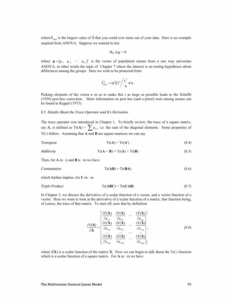
The Multivariate General Linear Model 89
where maxθ is the largest value of θ that you could ever mine out of your data. Here is an example inspired from ANOVA. Suppose we wanted to test H0: c′μ = 0 where ][ k21 ′μμμ= Lμ is the vector of population means from a one way univariate ANOVA, in other words the topic of Chapter 7 where the interest is on testing hypotheses about differences among the groups. Here we wish to be protected from
.ns)(ˆ
222
max ccyc ′′=t
Picking elements of the vector c so as to make this t as large as possible leads to the Scheffé (1959) post-hoc correction. More information on post hoc (and a priori) tests among means can be found in Keppel (1973).
8.5 Details About the Trace Operator and It's Derivative The trace operator was introduced in Chapter 1. To briefly review, the trace of a square matrix, say A, is defined as Tr(A) = ,a ii∑ i.e. the sum of the diagonal elements. Some properties of Tr(·) follow. Assuming that A and B are square matrices we can say Transpose Tr(A) = Tr(A′) (8.4) Additivity Tr(A + B) = Tr(A) + Tr(B) (8.5) Then, for A m · n and B n · m we have Commutative Tr(AB) = Tr(BA) (8.6) which further implies, for C m · m Triple Product Tr(ABC) = Tr(CAB) (8.7) In Chapter 3, we discuss the derivative of a scalar function of a vector, and a vector function of a vector. Here we want to look at the derivative of a scalar function of a matrix, that function being, of course, the trace of that matrix. To start off, note that by definition
,
x)(f
x)(f
x)(f
x)(f
x)(f
x)(f
x)(f
x)(f
x)(f
)(f
mn2m1m
n22221
n11211
⎥⎥⎥⎥⎥⎥⎥⎥
⎦
⎤
⎢⎢⎢⎢⎢⎢⎢⎢
⎣
⎡
∂∂
∂∂
∂∂
∂∂
∂∂
∂∂
∂∂
∂∂
∂∂
=∂
∂
XXX
XXX
XXX
XX
L
LLLL
L
L
(8.8)
where f(X) is a scalar function of the matrix X. Now we can begin to talk about the Tr(·) function which is a scalar function of a square matrix. For A m · m we have

90 Chapter 8
IA
A=
∂∂ )(Tr (8.9)
For A m · n and B n · m we can say
BAAB ′=
∂∂ )(Tr (8.10)
which also implies, from Equation (3.19)
BAAB
=′∂
∂ )(tr . (8.11)
Finally, assuming we have A m · m and B m · m,
ABBA
BAA )()(tr ′+=∂′∂ . (8.12)
8.6 The Kronecker Product We now review the definition of the Kronecker product, sometimes called the Direct product, with operator ⊗. By definition, a ijqpnmnqmp BBAC =⊗= . (8.13) For example,
.aa
babababababababa
bbbb
aa
21
11
22212121
12211121
22112111
12111111
2221
1211
21
11
⎥⎦
⎤⎢⎣
⎡=
⎥⎥⎥⎥
⎦
⎤
⎢⎢⎢⎢
⎣
⎡
=⎥⎦
⎤⎢⎣
⎡⊗⎥
⎦
⎤⎢⎣
⎡
BB
Here are some properties of the Kronecker product. We can say that Transpose (A ⊗ B)′ = A′ ⊗ B′. (8.14) For A m · n, B n · p and C p · q, it is the case that Associative AB ⊗ C = A ⊗ BC. (8.15) For A and B m · n and C p · q, Distributive (A + B) ⊗ C = A ⊗ C + B ⊗ C. (8.16)

The Multivariate General Linear Model 91
For A m · n, B n · p and C q · r and D r · s, (A ⊗ C)(B ⊗ D) = AB ⊗ CD. (8.17)
8.7 The Vec Operator For a matrix A, lets say m by n, we define
[ ].vec)(vec m21
m
2
1
⋅⋅⋅
⋅
⋅
⋅
′′′=
⎥⎥⎥⎥
⎦
⎤
⎢⎢⎢⎢
⎣
⎡
′
′′
= aaa
a
aa
A LL
(8.18)
While other definitions of Vec(·) are possible, this one, that does so one row at a time, will prove useful to us when we start to look at the multivariate GLM. In particular, the following theorem will be quite useful. For A m · n, B n · p and C p · q, Vec(ABC) = (A ⊗ C′) Vec(B). (8.19)
8.8 Eigenstructure for Asymmetric Matrices Suppose we needed to maximize x′Hx subject to x′Ex = 1. Then f(x) = x′Hx - λ(x′Ex -1) (8.20) and to minimize we set
.022)(f=λ−=
∂∂ ExHx
xx (8.21)
Rearranging a bit we have (H - λE)x = (E
-1H - λI)x = 0. (8.22)
You will note the eigenstructure discussed in Chapter 3 is a special case of the current discussion with E = I. In our case, as E
-1H is asymmetric, the eigenvectors are not orthonormal [defined in
Equation (3.33)]. Instead we have the relation E
-1H = XLX
-1 . (8.23)
For symmetric matrices we have had X
-1 = X′, but not in this case.
8.9 Eigenstructure for Rectangular Matrices For completeness, we note that any m ⋅ n matrix A or rank r can be decomposed into the triple product

92 Chapter 8
A = XL
1/2V′ (8.24)
where X is m ⋅ r, L
1/2 is r ⋅ r and V is n ⋅ r. This is called singular value decomposition. The
matrix X contains the left eigenvectors of A while V contains the right eigenvectors of A. Further, V′V = I and X′X = I. There are important relationships between the eigenvalues of a rectangular matrix and a cross product matrix. We have A′A = (XL
½V′) (VL
½X′) = XLX′ (8.25)
and AA′ = (VL
½U′) (UL
½V′) = VLV′ (8.26)
If A is already symmetric then A′A = AA′ so X = V.
8.10 The Multivariate General Linear Model The multivariate general linear model is a straightforward generalization of the univariate case in Equation (5.3). Instead of having one dependent variable in one column of the vector y, we have a set of p dependent variables in the several columns of the matrix Y. The model is therefore
⎥⎥⎥⎥⎥⎥⎥⎥⎥
⎦
⎤
⎢⎢⎢⎢⎢⎢⎢⎢⎢
⎣
⎡
βββ
βββ
βββ
⎥⎥⎥⎥⎥⎥⎥⎥⎥
⎦
⎤
⎢⎢⎢⎢⎢⎢⎢⎢⎢
⎣
⎡
=
⎥⎥⎥⎥⎥⎥⎥⎥⎥
⎦
⎤
⎢⎢⎢⎢⎢⎢⎢⎢⎢
⎣
⎡
p*k2*k1*k
p11211
p00201
*nk2n
*k221
*k111
npnpnp
p22221
p11211
xx1
xx1
xx1
yyy
yyy
yyy
L
LLLL
L
L
L
LLLL
L
L
L
LLLL
L
L
(8.27)
which, as you can see, implies that the number of columns of the B matrix match the number of columns of the Y matrix. Perhaps this concept is better represented using the dot subscript reduction operator (Section 1.1), which allows us to present the model as ][]ˆˆˆ[ p21p21 ⋅⋅⋅⋅⋅⋅ = βββXyyy LL (8.28) with each column of Y entering into a regression equation with the corresponding column of B serving as the coefficient vector. We can express the model most succinctly by using .ˆ XBY = (8.29) Next we define the n · p error of prediction matrix as ε, i. e. YY −= ˆε so that

The Multivariate General Linear Model 93
Y = XB + ε. (8.30)
8.11 A Least Squares Estimator for the MGLM How do we come up with estimators for the unknowns in the B matrix? When Y the error e was only a vector, as in Chapter 5, we could pick our objective function as e′e. The matrix ε′ε on the other hand, is not a scalar but a p · p sum of squares and cross products matrix. In this case what we do is to minimize the trace of ε′ε as we will now see. Our objective function is f = Tr[ε′ε] (8.31) which, according to Equation (8.30), can be expanded to f = Tr[(Y - XB)′ (Y - XB)]. (8.32) Factoring the product leads to four components as below; f = Tr[Y′Y - Y′XB - B′X′Y + B′X′XB]. But since Equation (8.5) notes that the trace of a sum is equivalent to the sum of the traces, we can now say f = Tr(Y′Y) - Tr(Y′XB) - Tr(B′X′Y) + Tr(B′X′XB). More simplification is possible. From Equation (8.4) we note that Tr(B′X′Y) = Tr(Y′XB) and from Equation (8.7) we note that Tr(Y′XB) is equivalent to Tr(BY′X). We can now rewrite f as f = Tr(Y′Y) - 2Tr(BY′X) + Tr(B′X′XB). In order to make f as small as possible, it is necessary to find the ∂f/∂B. Using Equations (8.10) as well as (8.12), we have
BXXXXYXB
])([2f ′′+′+′−=∂∂ .
But since X′X is symmetric, we can simplify a bit more and have
XBXYXB
′+′−=∂∂ 22f . (8.33)
After setting Equation (8.33) equal to zero, this now leads us to the multivariate analog of the normal equations [Equation (5.7)] as below: YXXBX ′=′ (8.34) so that YXXXB ′′= )(ˆ (8.35)

94 Chapter 8
Each column of B has the same formula as the univariate model, i. e. .)(ˆ
j1
j ⋅−
⋅ ′′= yXXXβ
8.12 Properties of the Error Matrix ε In order to talk about the distribution of the error matrix ε, we will have to rearrange it somewhat using the Vec(·) function of Section 8.7. We will assume, in a multivariate analog to the Gauss Markov Assumption of Chapter 5, that the distribution of the n by p matrix ε is ),(N~)(Vec ppnn1np ΣI0 ⊗ε . (8.36) The Vec operator has unpacked the ε matrix, one row at a time, in other words, one consumer's data at a time. Since there are n consumers with p measurements each, the mean vector of Vec(ε) is np by 1. The covariance matrix for Vec(ε), since the latter has np elements, must be np by np. This covariance matrix has a particular structure that logically, and visually, is reminiscent of the structure we assume in the univariate case presented in Equation (5.16), that of σ
2I = I · σ
2. Here,
instead we have the partitioned matrix
⎥⎥⎥⎥
⎦
⎤
⎢⎢⎢⎢
⎣
⎡
=⊗
Σ00
0Σ000Σ
ΣI
L
LLLL
L
L
(8.37)
with each Σ and each null matrix 0 being p · p. The Σ in the ith diagonal partition represents the (homogeneous) variance matrix for observation i. The 0 in the i, jth position implies that rows i and j of ε, corresponding to subjects i and j, are independent.
8.13 Properties of the B Matrix It is now timely to contemplate the expectation and variance of our estimator of Equation (8.35). Before proceeding, if you wish you can review some of the rules of expectations and variance presented in Section 4.1. The expectation will be straightforward, as ])[(E)ˆ(E 1 YXXXB ′′= − which for fixed X and Equation (4.5) leads to .)()(E)()ˆ(E 11 BXBXXXYXXXB =′′=′′= −− In order to derive the ),ˆ(V B we will need Theorem (4.9) as well as the more recent Theorem (8.19). OK, let us proceed by noting that .)()(ˆ 11 YIXXXYXXXB ′′=′′= −−

The Multivariate General Linear Model 95
Now with (X′X)
-1X′ playing the role of "A", Y playing the role of "B", and the p by p identity
matrix I playing the role of "C", we apply Theorem (8.19) to show that )(Vec])[()ˆ(Vec 1 YIXXXB ⊗′′= − Now we just need to recall that Var[Vec(Y)] = I ⊗ Σ and to apply Theorem (4.9) and take it to the bank: .])()[(])[()]ˆ(Vec[Var 11 IXXXΣIIXXXB ⊗′⊗⊗′′= −− (8.38) Note that in the above we have taken advantage of Equation (8.14) to express [(X′X)
-1X′ ⊗ I] ′ = X(X′X)
-1 ⊗ I .
Now applying Equation (8.17) two times to Equation (8.38) we can express it as .)()]ˆ(Vec[Var 1 ΣXXB ⊗′= − (8.39)
8.14 The Multivariate General Linear Hypothesis In Chapter 6 we looked at q degree of freedom hypotheses of the form H0: Aβ - c = 0, where the matrix A had q rows and where 0 is a q by 1 column of zeroes. In this chapter, since the B matrix has multiple columns of possible interest, as compared to β which is a column vector, we allow ourselves the possibility to test linear hypotheses about these several columns of B. The general form of the hypothesis is then H0: ABM - C = 0. (8.40) The q rows of A test hypotheses concerning the k independent variables. A is therefore q · k with q ≤ k. The l columns of M test hypotheses about the p dependent variables. M is necessarily p · l with l ≤ p. Next, in Section 8.15 we will look at some examples of A and M.
8.15 Some Examples of MGLM Hypotheses In our first example, we have k = 3 with x·0 being the usual column of 1's, x·1 being income, and then x·2 being education. On the dependent variable side, we have p = 2 with y·1 a measure of attitude towards a particular brand and y·2 being a likelihood of purchase measure. Imagine for a moment that we want to find out if education and income, taken jointly, impact the two dependent variables. Our hypothesis matrices would then take the form as shown below,

96 Chapter 8
⎥⎦
⎤⎢⎣
⎡
⎥⎥⎥
⎦
⎤
⎢⎢⎢
⎣
⎡
ββββββ
⎥⎦
⎤⎢⎣
⎡=
1001
100010
2212
1211
0201
ABM .
In the second example, k = 1 and x·0 is the usual vector of n 1's. However, p = 4 where y·1 through y·4 are evaluations of four product concepts on a 10 point scale. In this second example, the question of interest is, "Do the product evaluations differ?" In this case, we will use the multivariate approach to repeated measures. The current approach is in contrast to the univariate approach covered in Section 7.7. Here we have
⎥⎥⎥⎥
⎦
⎤
⎢⎢⎢⎢
⎣
⎡
−−
−
ββββ⋅=
111100010001
][1a 04030201BM .
Since there are no real independent variables, the matrix B is actually a row vector with only the intercepts present. In an intercept only model (see Section 5.9), the β0 values are simply the means of the dependent variables. The M hypothesis matrix transforms the four variable means into three mean-differences. Thus, the hypothesis is of three degress of freedom which test for equality among the levels of the four original dependent variables. Our example number 3 includes k = 4 with an intercept term plus three attitude variables. For dependent variables, we have p = 3 behavioral measures. Our hypothesis will be an omnibus question designed to ask whether attitude influences behavior:
IΑΒΜ⎥⎥⎥⎥
⎦
⎤
⎢⎢⎢⎢
⎣
⎡
ββββββββββββ
⎥⎥⎥
⎦
⎤
⎢⎢⎢
⎣
⎡=
333231
232221
131211
030201
100001000010
.
Finally, in our fourth example, we have experimental data in which we had a 2 × 2 ANOVA with four groups of consumers. Half the groups saw a high price, and half a low price. Half the groups saw the presence of advertising with half seeing no advertising. There is also the potential interaction of these two factors. Two measures were y·1; an affective response and y·2; a cognitive response. The hypothesis concerns the one degree of freedom interaction between price and advertising. Does such an interaction occur for affect and cognition?
⎥⎦
⎤⎢⎣
⎡
⎥⎥⎥⎥
⎦
⎤
⎢⎢⎢⎢
⎣
⎡
ββββββββ
=1001
]1000[
3231
2221
1211
0201
ABM .
8.16 Hypothesis and Error Sums of Squares and Cross-Products

The Multivariate General Linear Model 97
In the univariate linear model, we calculate the hypothesis sum of squares, which is a scalar that corresponds to the single dependent variable. The following equation produces the sum of squares and cross products matrix for the hypothesis embodied in Equation (8.40). As such, it is the multivariate analog to the univariate version presented in Equation (6.17): )ˆ(])([)ˆ( 11 CMBAAXXACMBAH −′′′−= −− . (8.41) The result is l by l with l being the number of columns of M and C, or in other words, the number of transformed dependent variables in the hypothesis in Equation (8.40). The error sums of squares and cross-products for the hypothesis, in contrast to the single sum of squares for the univariate version in Equation (5.22), is also an l · l matrix: E = M′ [Y′Y - Y′X(X′X)
-1X′ Y] M . (8.42)
Again in the univariate case, in Equation (6.18) we formed an F-ratio using the sum of squares for the hypothesis, and the sum of squares for the error. Modifying the form of Equation (6.18) somewhat, we can express the calculated F as
.q
knhekn/e
q/hkn/SS
q/SSF 1
Error
h −⋅=
−=
−= −
In the multivariate case we will do something similar, but the degrees of freedom are absorbed into the multivariate tables. But more importantly, since E
-1H is an l · l matrix, we must decide
how to summarize all of those numbers in a way that allows us to make an all-or-nothing decision about the hypothesis in Equation (8.40). Eigenstructure affords an optimal method for summarizing a matrix, and in Section 8.8 we studied the eigenstructure of asymmetric matrices like E
-1H. We are now ready to test our multivariate
linear hypothesis.
8.17 Statistics for Testing the Multivariate General Linear Hypothesis If we define s as the rank of E
-1H, we then have the eigenvalues λ1 , λ2 , ···, λs of the system
(E
-1H - λI)x = 0. (8.43)
In general, s = Min(q, l), that is, whichever is smaller, the number of rows of A or the number of columns of M. The eigenstructure of H(H + E)
-1 will be of interest also:
[H(H + E)
-1- θI]x = 0 (8.44)
with
i
ii 1 λ+
λ=θ (8.45)
so that

98 Chapter 8
.1 i
ii θ−
θ=λ (8.46)
In a logical sense, the λi are analogous to F ratios, being the eigenvalues of E
-1H, while the θi are
more analogous to squared multiple correlations, being the eigenvalues of H(H + E-1). Now there
are four different ways to test the multivariate hypothesis, proposed by four different statisticians. In addition, there is an F approximation that is somewhat commonly used as well. The four are:
Hotelling-Lawley Trace ∑λ=−s
ii
1 )(Tr HE (8.47)
Roy's Largest Root 1
11 1 λ+
λ=θ (8.48)
Pillai's Trace ∑∑ λ+λ
=θ=+ −s
i i
is
ii
1
1])([Tr EHH (8.49)
Wilk's Lambda ∏ λ+=
+=Λ
s
i i11
||||EH
H (8.50)
An especially good set of tables for these statistics can be found in Timm (1975). The F approximation is based on Wilk's determinantal criterion in Equation (8.50). That formula is
q
u2rt1F t/1
t/1
l−
⋅ΛΛ−
=′ (8.51)
where, as before, q is the number of rows or the rank of A, l is the number of columns or the rank of M, but there are some other parameters. The values
4
2qu −=
l ,
,1qknr2
l +−−−=
and n is the sample size while k is the number of columns of X. The degress of freedom for F′ are l · q in the numerator and rt - 2u in the denominator. The approximation is exact if s = Min(l, q) ≤
t =
l 2 q2 - 4 l 2 + q2 - 5
1
if l 2 + q2 – 5 > 0
if l 2 + q2 – 5 ≤ 0

The Multivariate General Linear Model 99
2, which is to say that the rank of E-1H is 2 or less. You will note the eigenstructure discussed in
Chapter 3 is a special case of the following discussion with E = I. Earlier, in Section 8.4, we spoke of correcting a statistical test for having a large number of tests and also for post hoc data snooping. If we consider the hypothesis H0: a′Bm = 0 where we try to pick the elements in the vectors a and m to make the significance test as large as possible, then maxθ , from Equation (8.3) is Roy's largest root. Unlike the Dunn-Bonferroni approach, the Union-Intersection approach controls for a high number of tests and also takes into account the correlations between the dependent variables. Another example would be where we try to maximize the correlation between a linear combination of x variables and a linear combination of the y variables. This is called canonical correlation.
8.18 Canonical Correlation In the multivariate general linear model, since there are p elements to the y vector and the k variables in the x vector, we face an embarrassment of riches in trying to summarize the relationship between the two sets of variables. Shown below, we see the partitioned matrix of all the variables, partitioned into y and x sets:
⎥⎦
⎤⎢⎣
⎡=
xxxy
yxyyRRRRR
The p · k matrix Ryx certainly has information in it about the relationship between the two sets of variables, containing as it does, the correlations between the sets. But in order to summarize the relationship between the two sets, we want a scalar. One obvious approach is to create new two new scores, one from the x set and one from the y set such that the correlation between the two scores is as high as possible. In essence, the problem is to pick the p elements of c′ in u = c′zy (8.52) and the k elements of d′ in v = d′zx (8.53) such that
dRdcRc
dcR
xxyy
2yx2 )(′⋅′
=ρ (8.54)
is maximized. This leads to two different eigenvector problems, 0]I[ 2
xy1
xxyx1
yy =ρ−−− cRRRR (8.55) and

100 Chapter 8
.0]I[ 2yx
1yyxy
1xx =ρ−−− dRRRR (8.56)
We can pick the smaller problem to solve and then deduce the other eigenvector using either
cRRd xy1
xx2
1 −
ρ= (8.57)
or
.1yx
1yy2 dRRc −
ρ= (8.58)
The canonical correlation can be thought of as a linear hypothesis of the form of Equation (8.40) with
kAk* ][
1000
01000010
*k*k1k I0=
⎥⎥⎥⎥
⎦
⎤
⎢⎢⎢⎢
⎣
⎡
=
L
LLLLL
L
L
and M = pIp. The number of canonical correlations and eigenvector combinations depends on s, which in this case is simply whichever is smaller, k or p. The first canonical correlation squared corresponds to Roy's Largest Root in Equation (8.48), which can be used to test the hypothesis that the canonical correlation is zero. One can also use Pillai's Trace [Equation (8.49)] to test whether all of the canonical correlations are zero, i. e. H0: .02
s22
21 =ρ==ρ=ρ L
Placing each of the eigenvectors, a·1, a·2 , ···, a·s into columns of the matrix A (not the hypothesis matrix), we have rows of A that correspond to y variables and columns of A that correspond to different canonical variables from Equation (8.52). We can standardize the elements of A using Cs = C(C′RyyC)
-1/2
and for the x set we have Ds = D(D′RxxD)
-1/2.
It is also instructive to look at the correlations between each of the canonical variables in Equation (8.53) and the variables of the x set, and the canonical variables in Equation (8.52) and the variables of the y set. We have for each combination ,),(Cov yysy RCzu ′= ,),(Cov xxsy RDzv ′= ,),(Cov yxsx RCzu ′=

The Multivariate General Linear Model 101
.xysy ),(Cov RDzv ′=
8.19 MANOVA We will begin with an example with a purely between subjects design, and two different dependent variables. Imagine that we have four groups of subjects, each group having seen a different advertisement. Thus, k = 4 with x·0 being the usual vector of constants and x·1, x·2 and x·3 coding for group membership. To keep things simple, lets say that y·1 contains the respondent's answer to the question, "How much do you like the product?" while y·2 has data on "Intention to buy." In summary, Y is n · 2, X is n · 4 and B is 4 · 2 with .ˆ XBY = It would be natural to test the hypothesis of no group differences for the two dependent variables. This hypothesis is much the same as canonical correlation, its just that the emphasis is slightly different. We calculate the hypothesis sum of squares and cross product matrix ),ˆ(])([)ˆ( 11 CMBAAXXACMBAH −′′′−= −− with
⎥⎥⎥
⎦
⎤
⎢⎢⎢
⎣
⎡=
100001000010
A
and M = 2I2 and the error sum of squares and cross products matrix, E = M′ [Y′Y - Y′X(X′X)
-1X′ Y] M,
invert this latter matrix in order to find the eigenvalues of E
-1H, calculate the four criteria and the
F approximation, and see to the fate of H0. In addition, the eigenvectors for the y set, v = d′y, can tell us the optimal combination of y's for detecting group differences. Similarly, the eigenvectors for the x set reveal the best possible contrast among the group means.
8.20 MANOVA and Repeated Measures To start off this section, we will pick an example with no grouping variables, just one group of consumers who rate a product using the same scale under p = 3 different scenarios. The multivariate model is then
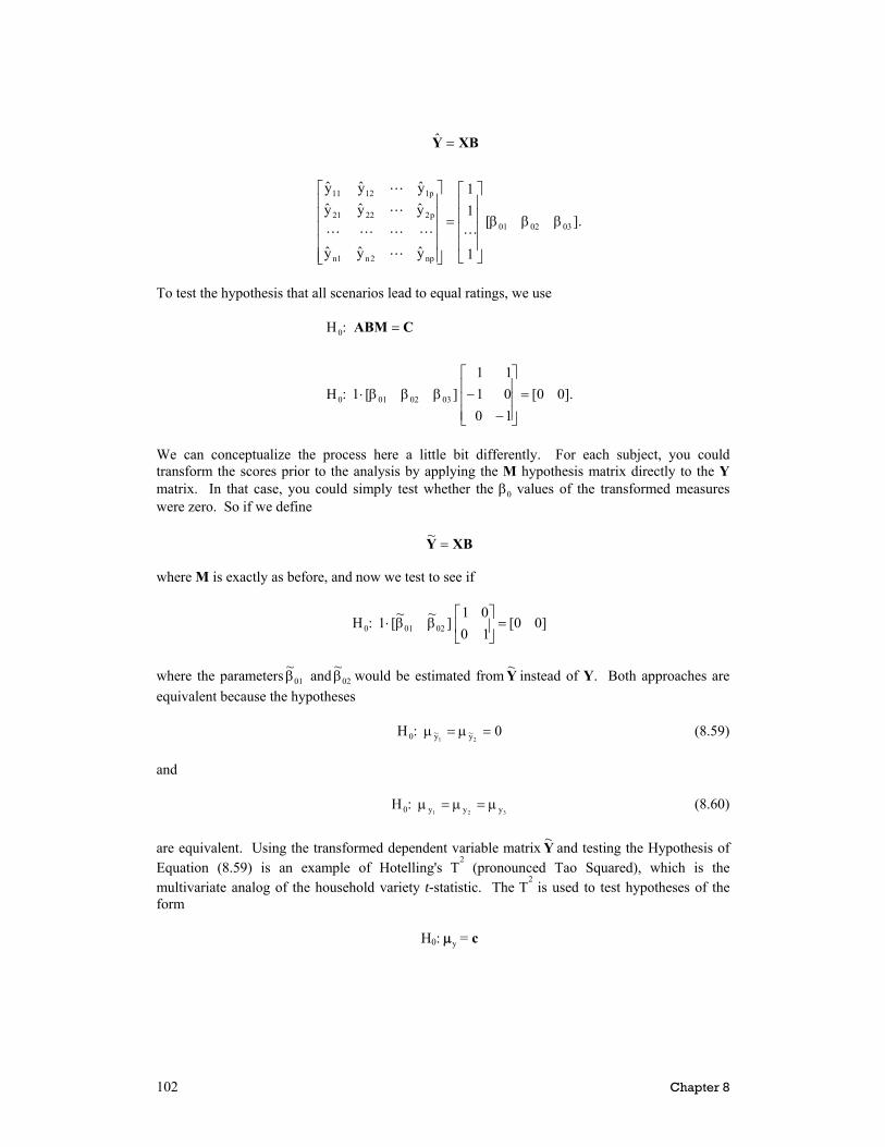
102 Chapter 8
].[
1
11
yyy
yyyyyy
ˆ
030201
np2n1n
p22221
p11211
βββ
⎥⎥⎥⎥
⎦
⎤
⎢⎢⎢⎢
⎣
⎡
=
⎥⎥⎥⎥⎥
⎦
⎤
⎢⎢⎢⎢⎢
⎣
⎡
=
L
L
LLLL
L
L
XBY
To test the hypothesis that all scenarios lead to equal ratings, we use
].00[100111
][1:H
:H
0302010
0
=⎥⎥⎥
⎦
⎤
⎢⎢⎢
⎣
⎡
−−βββ⋅
= CABM
We can conceptualize the process here a little bit differently. For each subject, you could transform the scores prior to the analysis by applying the M hypothesis matrix directly to the Y matrix. In that case, you could simply test whether the β0 values of the transformed measures were zero. So if we define XBY =
~ where M is exactly as before, and now we test to see if
]00[1001
]~~[1:H 02010 =⎥⎦
⎤⎢⎣
⎡ββ⋅
where the parameters 01
~β and 02
~β would be estimated from Y~ instead of Y. Both approaches are
equivalent because the hypotheses 0:H
21 y~y~0 =μ=μ (8.59) and
321 yyy0:H μ=μ=μ (8.60) are equivalent. Using the transformed dependent variable matrix Y~ and testing the Hypothesis of Equation (8.59) is an example of Hotelling's Τ
2 (pronounced Tao Squared), which is the
multivariate analog of the household variety t-statistic. The Τ2 is used to test hypotheses of the
form H0: μy = c

The Multivariate General Linear Model 103
with μy being the vector of population means for the dependent variables. Hotelling's Τ2can also
be used to test multivariable mean differences across two groups, just as the t does where there is but one dependent variable. Now we put together an example where there are different groups of subjects as well as repeated measurements. As before, we assume that all subjects rate a product under p = 3 different scenarios. But now there are actually four different treatment groups, each group having seen a different advertisement for the product. In that case, k = 4 so that the B matrix is 4 by 3. Each column of B corresponds to one of the three rating scenarios. The first row of B contains the intercept terms, while the next three rows pertain to group differences. Is there an impact of advertisement? In the univariate approach, we add up the three measures to create for each subject i, y~ = y1 + y2 + y3. We test the hypothesis using cβA =
~:H0
⎥⎥⎥
⎦
⎤
⎢⎢⎢
⎣
⎡=
⎥⎥⎥⎥⎥
⎦
⎤
⎢⎢⎢⎢⎢
⎣
⎡
ββββ
⎥⎥⎥
⎦
⎤
⎢⎢⎢
⎣
⎡
000
~~~~
100001000010
:H
3
2
1
0
0 .
which is covered in Chapter 7. In the multivariate approach covered in this chapter, we do not transform the dependent variables, we leave them as they are. We have CABM =:H0
.000000000
100001000010
:H
333231
232221
131211
030201
0
⎥⎥⎥
⎦
⎤
⎢⎢⎢
⎣
⎡=
⎥⎥⎥⎥
⎦
⎤
⎢⎢⎢⎢
⎣
⎡
ββββββββββββ
⎥⎥⎥
⎦
⎤
⎢⎢⎢
⎣
⎡I
This approach confounds the main effect of group with the simple main effect of advertisement on y·1 , on y·2 and on y·3. In other words, from column 1 of Y we look to see what effect there is of group membership, we do the same thing with columns 2 and 3. But this claims some of the variance that would ordinarily be considered part of the advertisement × scenario interaction. The main effect of advertisement would generally look only at a summary of the group differences holding the scenario constant. Is there an effect of scenario? Here we start with the univariate approach. If we define
⎥⎥⎥
⎦
⎤
⎢⎢⎢
⎣
⎡
−−=
100111
M
and assume that IΣMM 2σ=′

104 Chapter 8
as we did in Equation (7.12), we can utilize the univariate approach to repeated measures and use the F-test discussed in Section 7.7 with an error term of subjects × scenario interaction. In the univariate approach all scores are placed in a single column vector. In contrast, in the multivariate case each scenario constitutes a different column of Y and we test CABM =:H0
[ ] [ ].0010
0111
0001:H
333231
232221
131211
030201
0 =⎥⎥⎥
⎦
⎤
⎢⎢⎢
⎣
⎡
−−
⎥⎥⎥⎥
⎦
⎤
⎢⎢⎢⎢
⎣
⎡
ββββββββββββ
There also exists an approach in between the univariate and multivariate methods. One could Test IΣMM 2
0:H σ=′ and pick the univariate approach if you fail to reject and the multivariate approach if you reject. Another approach was proposed by Greenhouse and Geisser (1959) who suggested that we could correct the univariate F to the degree that .ˆ 2ISMM σ≠′ (8.61) Here in Equation (8.61) we have replaced Σ with it's estimator, S. If we wish to test the advertisement × scenario interaction according to the univariate approach, we would need to assume that M′ΣM = σ
2I, place all scores in the vector y, and use the interaction
of subjects × scenario as the error term. In order to test the advertisement × scenario interaction according to the multivariate model, we can combine the A matrix from the advertisement main effect and the M matrix from the scenario main effect. In that case we have CABM =:H0
.000000
100111
100001000010
:H
333231
232221
131211
030201
0
⎥⎥⎥
⎦
⎤
⎢⎢⎢
⎣
⎡=
⎥⎥⎥
⎦
⎤
⎢⎢⎢
⎣
⎡
−−
⎥⎥⎥⎥
⎦
⎤
⎢⎢⎢⎢
⎣
⎡
ββββββββββββ
⎥⎥⎥
⎦
⎤
⎢⎢⎢
⎣
⎡
8.21 Classification To motivate this section, which will discuss the technique known as the discriminant function, we begin the discussion with a little two group example. Imagine we are trying to decide who to include in direct mailing. Our goal is to classify our customers into two groups based on whether they will, or will not, respond to the mailout. From a sample of our customer base, we have collected some data which we will get to in just a minute. For now, we note that the cost, or

The Multivariate General Linear Model 105
disutility, of misclassifying someone in group i, mistakenly placing them in group j is cij. Given our two groups, we might then tabulate the cost matrix as
Classification Decision Group 1 Group 2
Group 1 0 c12 Reality Group 2 c21 0 For each individual we have a p element row vector from the matrix Y, ,i⋅′y containing numeric variables. The probability density for the individuals in group j is fj(yi·), while πj is the relative size of group j, also called the prior probability. The conditional probability an individual with vector yi· comes from group j is
∑ ⋅
⋅⋅
π
π=
mimm
ijji
)(f
)(f)|jPr(
y
yy
We want to minimize our expected cost which in the two group case is given by 21i12i c)|2Pr(c)|1Pr( ⋅⋅ + yy and we can decide that individual is in group 1 if f1(yi·) · π1 · c12 > f2(yi·) · π2 · c21
or rearranging we can say that we should decide that the individual is in group 1 if
.cc
)(f)(f
12
21
1
2
i2
i1 ⋅ππ
>⋅
⋅
yy (8.62)
If the πj are unknown or assumed to be equal, and c21 = c12, then it is only the right hand side of the above Equation (8.62) and what matters is the relative height of the two densities. The crossover point of Equation (8.62) would be the place where the densities themselves cross over. The usual assumption is that an observation vector from group j yi· ~ N(μj, Σj) which implies from Equation (4.17) that
[ ]2/)()(exp)2(||
1)(f ji1
jji2/p2/1j
ii μyΣμyΣ
y −′−−π
= ⋅−
⋅⋅ .
Taking Equation (8.62) and taking logs to both sides, we would then place a case in group 1 if
121
212
i2
i1
ccln
)(f)(fln
ππ
>⋅
⋅
yy

106 Chapter 8
[ ] .ccln)()()()(
21
||||ln
21
121
2122i
122i1i
111i
1
2
ππ
>−′−−−′−− ⋅−
⋅⋅−
⋅ μyΣμyμyΣμyΣΣ
If we assume that Σ1 = Σ2 = Σ the above expression simplifies to
[ ] [ ] .ccln)()(
21)(y
121
21221
12121
1i π
π>−μ′+−−′ −−
⋅ μΣμμμμΣ (8.63)
To get to this point it helps to realize that (a - b)′C(a - b) = a′Ca - 2a′Cb + b′Cb and that (a +
b)′C(a - b) = a′Ca - b′Cb. Noting also that ,abln
baln −= if we substract
121
212
ccln
ππ from both sides
of the above equation we get
[ ] [ ] .0ccln)()(
21)(y
121
21221
12121
1i >
ππ
−−′+−−′ −−⋅ μμΣμμμμΣ (8.64)
Define the left hand side of this last equation as ν12. Our decision to place a case in group 1 is made if ν12 > 0. For population 1 we have
⎟⎟⎠
⎞⎜⎜⎝
⎛ΔΔ+
ππ
ν 212
212
212
12112 ,
cc
lnN~
where )()( 21
121
212 μμμμ −Σ′−=Δ −
which is known as the Mahalanobis distance between the mean vectors of the two populations. Knowing the distribution of ν12 allows us to estimate the probability and the total costs of misclassification. We also define the raw discriminant function as ν = d′yi· where d = Σ
-1(μ1 - μ2).
We can also standardize the function using ⋅⋅
− ′=′Δ=ν isi1
12s ydyd Back to the decision,

The Multivariate General Linear Model 107
[ ] [ ]
.0)(21
cc
ln
0)()(21)(y
cc
ln
21i121
212
211
21211
i121
212
>′+−′+ππ
>−′+−−′+ππ
⋅
−−⋅
dμμdy
μμΣμμμμΣ
Rearranging, our decision "1" is taken if
121
21221i c
cln)(21
ππ
−′+>′=ν ⋅ dμμdy
or in the standardized version
121
212112s21sis c
cln)(21
ππ
Δ−′+>′=ν −⋅ dμμdy .
The discriminant function maximizes the separation between the values ,and 21 νν the means for the two groups on the discriminant scores. When we don’t know the μj or Σ, we split our samples into validation and holdout samples.
8.22 Multiple Group Discriminant Function The problem can be approached as a special case of MANOVA. For example, assuming that we have k = 4 groups with p discriminating dependent variables, and the general linear hypothesis H0: ABM = 0, we would use the hypothesis matrix
⎥⎥⎥
⎦
⎤
⎢⎢⎢
⎣
⎡=
100001000010
A
with M = I. Just as we did before in Equations (8.41) and (8.42), we would calculate the hypothesis and error sum of squares matrices H and E. In order to find a score, ν = d′yi·, with ν have as large a between groups sum of squares as possible, we will utilize the eigenstructure of
HE 1− as before. We pick values in the vector d such that our F test for group differences on ν is as large as possible. In other words, we maximize the between groups sum of squares for ν
divided by it's within groups sum of squares, that is to say ,EddHdd′′
over all possible values of a. It
is customary to scale a such that the within-group variance (mean square) is
.1kn
=′=−′
SddEdd

108 Chapter 8
References Greenhouse, Samuel W. and S. Geisser (1959) On Methods in the Analysis of Profile Data. Psychometrika, 24, 95-112. Hair, Joseph F., Rolph E. Anderson, Ronald L. Tatham and William C. Black (1995) Multivariate Data Analysis. Fourth Edition.. Englewood Cliffs, NJ: Prentice-Hall. Keppel, Geoffrey (1973) Design and Analysis: A Researcher's Handbook. Englewood Cliffs, New Jersey: Prentice-Hall. Lattin, James, J. Douglas Carroll and Paul E. Green (2003) Analyzing Multivariate Data. Pacific Grove, CA: Brooks/Cole. Marascuilo, Leonard A. and Joel R. Levin (1983) Multivariate Statistics in the Social Sciences. Monterey, CA: Brooks/Cole. Scheffé, Henri (1959) The Analysis of Variance. New York: Wiley. Sharma, Subhash (1996) Applied Multivariate Techniques. New York: Wiley Tatsuoka, Maurice M. (1971) Multivariate Analysis. New York: Wiley. Timm, N. H. (1975) Multivariate Analysis with Applications in Education and Psychology. Monterey, CA: Brooks/Coles.

109
Section III: Covariance Structure

110 Chapter 9
Chapter 9: Confirmatory Factor Analysis Prerequisites: Chapter 5, Sections 3.9, 3.10, 4.3
9.1 The Confirmatory Factor Analysis Model The difference between the models discussed in this section, and the regression model introduced in Chapter 5 is in the nature of the independent variables, and the fact that we have multiple dependent variables. The independent variables are unobserved constructs, also known as factors, dimensions or latent variables. At this point the student might ask, how scientific is it to speak of unobserved variables in a model? We will soon see that if the model of unobserved independent variables is correct, it makes a strong prediction about the structure of the covariances among the observed dependent variables. For this reason, these models are a special case of models known as covariance structure models. Given that we are dealing with unobserved variables, it will be useful to shift our notation somewhat. In regression, we look at a particular variable as a column vector that displays the individual observations which comprise the rows. In factor analysis, the individual observations cannot be fully observed since the right hand side variables, the factors, are not observed. Instead, we will propagate our model using a typical observation, call it observation i, but leaving off the subscript i. What’s more, instead of arranging our matrices such that the each column is a different variable and each row is a different observation, we will be looking at the transpose. Of course, this is in contrast to the notation employed in Chapters 5 through 8. In that later chapter, we study the model Y = XB + ε where the columns of Y (and the parameter vector B as well as the error matrix ε) represent the p different dependent variables. If we were to take the transpose of both sides of that model we would have Y′ = B′X′ + ε′. You will note that, since the product of a transpose is the transpose of the product in reverse order [Equation (1.34)], B and X are now reversed. Also, the data matrices Y′ and X′ now have a row for each variable, instead of a column as before. Next, as described above, rather than look at every subject, we look at a typical observation, for example, number i: .iii ⋅⋅⋅ +′= εxBy The dot, which is a subscript reduction operator, is mentioned in Section 1.1. One final change is convenient. If we totally drop the subscripts from ,and, iii ⋅⋅⋅ εxy we would just have y = B′x + ε. This is how we will describe the model in this chapter. We will call the regression weights λ's instead of β's and the independent variables will be η's instead of x's. We start out with a scalar representation of the situation:

Structural Equation Models 111
.εηληληλy
εηληληλyεηληληλy
pmpm22p11pp
2mm22221212
1mm12121111
++++==
++++=++++=
L
LL
L
L
(9.1)
The left hand side shows p different variables. Perhaps y1 through y3 represent three measures of consumer “greenness”, that is, a tendency to buy environmental friendly products. Perhaps y4 through y6 represent three different measures of innovativeness. In any case, the point is that the y’s are p manifest or observed variables. As has been mentioned, we are representing the data from a typical subject, the i-th, but the subscript i is left off according to the traditions in this area. On the right hand side, you have regression coefficients, the λij, which are basically β weights. In the context of factor analysis, regression weights are called factor loadings. The reason that they have two subscripts is that you need one subscript to keep track of the dependent variable, or the equation, and another subscript to keep track of the independent variable. And speaking of which, these are the η values of which there are m. The η’s are the common factors which explain much of the behavior of the y’s, at least the part of their behavior that they have in common – the covariances. Finally, we have the εi which are called unique factors. This is not exactly the same thing as the error in a regression model. In regression, the error is an error-in-equations, also called specification error. That is to say, unless a regression model has an R2 of 1, the model is missing some explanatory independent variables or is otherwise mispecified. In factor analysis, the ε’s are errors-in-variables, or measurement error. The three variables we devised to measure “greenness”, for example, might not do so perfectly. We generally assume that the part that the three variables have in common, as quantified by their covariances, must be due to the fact that all three are at least partially measuring what they are supposed to be measuring. But each one of the three has some variance that is unique to it. That is what the εi account for. We can write the model in matrix terms,
.
y
yy
p
2
1
m
2
1
pm2p1p
m22221
m11211
p
2
1
⎥⎥⎥⎥⎥
⎦
⎤
⎢⎢⎢⎢⎢
⎣
⎡
ε
εε
+
⎥⎥⎥⎥
⎦
⎤
⎢⎢⎢⎢
⎣
⎡
η
ηη
⎥⎥⎥⎥⎥
⎦
⎤
⎢⎢⎢⎢⎢
⎣
⎡
λλλ
λλλλλλ
=
⎥⎥⎥⎥⎥
⎦
⎤
⎢⎢⎢⎢⎢
⎣
⎡
LL
L
LLLL
L
L
L
.ε+= Ληy (9.2) By all rights, in addition to the y vector, the η and ε vectors should have a subscript i since they are random variables, sampled from the population for which this model holds. On the other hand, Λ is a constant matrix, holding parameters that describe this population. So how does this model with unobserved variables make contact with reality? In order to show how it does so, we need to start with some assumptions and some definitions. We will assume that E(y) = 0, a p by 1 null vector. This does not reduce the generality of the model at all, since covariances are not affected by the addition or subtraction of a constant [see Theorem (4.8)]. In order to estimate the model, we will make the assumptions that η ~ N(0, Ψ), ε ~ N(0, Θ)

112 Chapter 9
and that Cov(ε, η) = 0. Like the y vector, η and ε are mean-centered. We will also see quite a bit of the coviarance matrices for η and ε, with V(η) = Ψ and V(ε) = Θ. At this point, we are ready to see what the covariance matrix of the y’s should look like. We have by the definition of variance in Equation (4.7)
[ ]
),(E)(E)(E)(E
))((E
)(E)(V
εεΛηεεηΛΛηηΛ
εΛηεΛη
yyΣy
′+′′+′+′′=
′++=
′=≡
but of the four components from left to right, pieces two and three vanish since Cov(ε, η) = 0. We have made use of Equation (4.5) and (4.6). We can rewrite E(ηη′) = Ψ, which was defined above as the covariance matrix of the η's when we were talking about assumptions. In piece four we have E(εε′) = Θ which was also defined above as the variance of the unique factors. Putting all of these conclusions together, we end up with the fact that the variance of y is V(y) = ΛΨΛ′ + Θ . (9.3)
9.2 A Confirmatory Factor Analysis Example Now is the section of the chapter where we look at an example confirmatory factor analysis that is just complicated enough to be a valid example, but is simple enough to be, well; a silly example. Lets say we have devised three questionnaire items which measure the consumers’ attitude towards Beer B, and three other items that measure attitudes towards Beer C. Our six item survey then contains the variables listed in the table: To finish describing the model, we will hypothesize that there are two factors, B (η1) and C (η2). Our model would then look like
Variables Description y1 Measurement 1 of B y2 Measurement 2 of B y3 Measurement 3 of B y4 Measurement 1 of C y5 Measurement 2 of C y6 Measurement 3 of C

Structural Equation Models 113
⎥⎥⎥⎥⎥⎥⎥⎥
⎦
⎤
⎢⎢⎢⎢⎢⎢⎢⎢
⎣
⎡
εεεεεε
+⎥⎦
⎤⎢⎣
⎡ηη
⎥⎥⎥⎥⎥⎥⎥⎥
⎦
⎤
⎢⎢⎢⎢⎢⎢⎢⎢
⎣
⎡
λλλ
λλλ
=
⎥⎥⎥⎥⎥⎥⎥⎥
⎦
⎤
⎢⎢⎢⎢⎢⎢⎢⎢
⎣
⎡
+=
6
5
4
3
2
1
2
1
62
52
42
31
21
11
6
5
4
3
2
1
000
000
yyyyyy
εΛηy.
Again, remember that the y, η and ε vectors are random variables, but Λ is a parameter matrix and the unknowns in it must be estimated from the sample. To fully estimate the model, we also have two other parameter matrices,
.
00
00
00
and
pp
22
11
2221
11
⎥⎥⎥⎥⎥⎥
⎦
⎤
⎢⎢⎢⎢⎢⎢
⎣
⎡
θ
θ
θ
=
⎥⎥⎦
⎤
⎢⎢⎣
⎡
ψψ
−ψ=
L
LLLL
L
L
Θ
Ψ
Note that the Ψ matrix is symmetric, being a covariance matrix and so we do not need to enumerate the upper triangular part of it. And by the definition of what we mean by a unique factor, the εi are independent which means that the variance matrix of the εi, Θ, is diagonal. As a general rule in covariance structure models, we need to specify variances and covariances of right hand side random variables, and we need to specify regression weights between right hand and left hand side variables. Below you can see what we call the Path Diagram for this model:
A path diagram is a very common way of representing a covariance structure model, and there are a set of conventions that go along with this type of figure. Single-headed arrows represent directional causal pathways, and two-headed arrows are used to represent covariation. Unique
y2
y3
y4
y5
y6
y1
η1 η2
λ11
λ21
λ31
λ42
λ52
λ62
ψ21

114 Chapter 9
factors, and other sorts of error terms, are usually indicated by single-headed arrows without labels. Circles are used to convey the presence of latent variables, and boxes convey observed variables.
9.3 Setting a Metric for Latent Variables The model as it has been presented so far cannot be uniquely identified. To illustrate this, lets pretend we have a single variable and a single factor. In that case everything boils down to scalars, and the model is y = λη + ε and from Equation (9.3), V(y) = λ2ψ + θ. Now define η* = a·η so that V(η*) = a2ψ =ψ*. Also, define λ* = λ/a. In that case,
alsoandaa
**y ε+η⋅λ
=ε+ηλ= (9.4)
.aa
**)y(V 22
22 θ+ψ⋅
λ=θ+ψλ= (9.5)
What this means is that if I have a model with parameters λ* and ψ*, and you have a model with parameters λ and ψ, both models would fit equally well and there would be no logical way to decide which was better. In fact, they would be completely equivalent. The source of this ambiguity lies in the fact that η is unobserved, and it is at most an interval scale. To further identify the model we must set intervals for it, a process called setting its metric. We can do this in one of two ways. We can fix one loading per factor to a constant, such as 1.0, or we can fix the variance of each factor to 1.0. Returning to our two factor example, the first method would yield
⎥⎦
⎤⎢⎣
⎡ψψ−ψ
=
⎥⎥⎥⎥⎥⎥⎥⎥
⎦
⎤
⎢⎢⎢⎢⎢⎢⎢⎢
⎣
⎡
λλ
λλ
=2221
11
62
52
31
21
and,
00
100001
ΨΛ
while the second approach would give
.1
1and,
000
000
21
62
52
42
31
21
11
⎥⎦
⎤⎢⎣
⎡ψ
−=
⎥⎥⎥⎥⎥⎥⎥⎥
⎦
⎤
⎢⎢⎢⎢⎢⎢⎢⎢
⎣
⎡
λλλ
λλλ
= ΨΛ
These two methods are equivalent, yielding the same Chi Square values, but the first method is slightly more general, being applicable in certain situations where the second method cannot be used. The first method ties the metric of each factor to the first variable that measures it. The second method turns the factors into z-scores, and the factor covariance matrix Ψ can then be interpreted as a correlation matrix. For both methods, the Θ matrix has p free parameters.

Structural Equation Models 115
9.4 Degrees of Freedom for a Confirmatory Factor Analysis Model Factor analysis does not look directly at raw data. The input data for this technique are the elements of the sample covariance matrix S, which is a p by p symmetric matrix. Therefore S contains
2
)1p(p + (9.6)
“data points”, those being the p variances and the p(p-1)/2 unique covariances. For our 6 variable example, this would total 21. In our model, assuming we use the first method to fix the metric of the two factors, we have 4 λ’s 3 ψ’s 6 θ’s ------- 13 parameters The degrees of freedom for the model are equal to the number of data points minus the number of unique free parameters that are estimated from those data. In our case, we have 21 – 13 = 8 degrees of freedom. We will be able to reject the model (or not as the case may be) using a χ2 test with 8 degrees of freedom. In terms of hypotheses, we will be testing H0: Σ = ΛΨΛ′ + Θ (9.7) against the general alternative HA: Σ = S . (9.8) In some ways this pair of hypotheses is very similar to hypotheses that we saw in Chapter 6 with regression. However, here we have a different sort of emotional attachment to the hypotheses. In regression, which encompasses everything from the basic t-test through more complex possibilities, we are generally motivated to “hope for” HA and hope against H0. Here, our model is H0, so in an emotional sense, the roles of the Type I and II errors are reversed. The truth is that the current situation is actually more natural, if we can use that word. In regression, the hypothesis we are testing is a sort of “straw man” that no one believes in anyway, and that we set up just to knock down. We will talk more about the “emotional reversal” of H0 and HA later when we discuss goodness of fit measures (that is, measures other than the traditional χ2). But first, it is time to understand how we estimate the parameters of the model and come up with a χ2 value to test it. That is the topic of the next two sections. We will be using an estimation philosophy known as Maximum Likelihood. In order to explore this topic, we will be returning to the much simpler regression model. Then we will venture forth and look at estimation for confirmatory factor analysis models.
9.5 Maximum Likelihood Estimators for Factor Analysis Maximum likelihood is discussed in general in Section 3.10 and within the context of the regression model in Section 5.4. ML for factor analysis begins with the probability of observation i under the confirmatory factor analysis model. Here we have the multivariate normal distribution

116 Chapter 9
[see Equation (4.17)] to deal with since we have p variables, not just one as we did with regression. We have
⎥⎦⎤
⎢⎣⎡ ′−
π= −
⋅ i1
i2/12/pi 21exp
||)2(1)Pr( yΣyΣ
y (9.9)
for the p variables on observation i. For the whole sample we have
.21exp
||)2(1)yPr(
n
ii
1i2/n2/np
n
ii0
⎥⎥⎦
⎤
⎢⎢⎣
⎡′−
Σπ== ∑∏ − yΣyl (9.10)
The summation in the exponent of the above equation makes sense if you keep in mind that e
a · e
b
= ea+b
. Now, to get ready for the next equation note that from Equation (1.27) and Section 1.7
]n[tr 1i
1n
ii
−− =′′∑ SΣyΣy (9.11)
because
]n[TrTrTr 11n
iii
1i
n
ii
1i
−−−− =′=⎥⎥⎦
⎤
⎢⎢⎣
⎡′=′ ∑∑∑ SΣΣyyyΣyyΣy i .
This is so since a scalar is equal to its trace, and the trace of a product is invariant to the sequence of that product assuming conformability. We now take the log of the likelihood in Equation (9.10) but substitute the identity from Equation (9.11) to end up with
[ ].)(tr||lnn21ttancons
)(trn21||lnn
21)2(lnpn
21Lln
1
100
−
−
+−=
−−π−==
SΣΣ
SΣΣl
(9.12)
The term "constant" above represents )2(lnpn21
π− which doesn't impact the optimal solution
one way or the other since it does not depend on the parameters and so will not figure into the derivative. Now suppose I look at the likelihood under HA: Σ = S. We will call that log likelihood LA and we find that
LA = constant - [ ]p||lnn21
+S . (9.13)
Now we have two log likelihoods, one; L0 which reflects the confirmatory factor analysis model, and another that gives us the log likelihood under the general alternative that Σ exhibits no particular structure, which is to say it is arbitrary. In other words, it is what it is. It turns out that under very general conditions,

Structural Equation Models 117
[ ] )m(~LL2ln2 2A0
A
0 χ−−=⎥⎦
⎤⎢⎣
⎡−
l
l, (9.14)
where m represents the difference in the number of parameters estimated under the two models; the null (0) and the alternative (A). As we have already described, the alternative model estimates
2)1p(p + parameters while the number of parameters in the null model depends on the specific
theory as expressed in the matrices Λ, Ψ and Θ. Plugging Equations (9.12) and (9.13) into Equation (9.14), the χ2 value is then [ ]p)(tr||ln||lnnˆ 12 −+−=χ −SΣSΣ . (9.15) As can be seen, as Σ → S, →χ2ˆ 0. Thus the closer the match between Σ and S, the smaller the
value of χ2. But it is also true that as n → ∞, →χ2ˆ ∞, and conversely, as n → 0, →χ2ˆ 0. This means that all things being equal, it becomes easier to reject H0 the larger the sample size, and it becomes harder to reject H0 the smaller the sample size. This is how all efficient statistics function, but since we have an emotional attachment to H0 instead of HA, this would seem to have certain consequences both for individual researchers, and for the development of marketing as a whole. It is necessary that we pick values for the unknowns in the matrices Λ, Ψ and Θ at the minimum value of Equation (9.15). Equation (9.15) is obviously nonlinear in the unknowns so this will entail nonlinear optimization as discussed in Section 3.9. For now we note that any computer algorithm that finds the minimum of Equation (9.15) will utilize the derivatives of that function to determine "which way is down". Any such algorithm, however, requires rational starting values to avoid ending up in a local, rather than the global, minimum of the function. As such, you should do the best job that you can by manually inserting starting values into whatever program you use to estimate the confirmatory factor model. Certainly, under any circumstances, you should be able to get the sign right for any loadings in the matrix Λ. Diagonal elements of Θ could be seeded with small positive values. Diagonal elements of Ψ are likely to resemble the variances of the measures, while off-diagonal elements could be smaller than the diagonal, and of appropriate sign. Of course, it is also important that any fixed elements in the matrices Λ, Ψ and Θ have appropriate starting values, as these will also end up as the final values!
9.6 Special Case: The One Factor Model Consider a confirmatory factor model with one factor:
.
y
y
y
p
2
1
p
2
1
p
2
1
⎥⎥⎥⎥⎥⎥
⎦
⎤
⎢⎢⎢⎢⎢⎢
⎣
⎡
ε
ε
ε
+η
⎥⎥⎥⎥⎥⎥
⎦
⎤
⎢⎢⎢⎢⎢⎢
⎣
⎡
λ
λ
λ
=
⎥⎥⎥⎥⎥⎥
⎦
⎤
⎢⎢⎢⎢⎢⎢
⎣
⎡
LLL
If we fix V(η) = ψ11 = 1, the expression for the covariance matrix is simply Σ = λλ′ + Θ (9.16)

118 Chapter 9
and our measures y1 , y2 , …, yp are called congeneric tests. In this context the single η is called a true score. As you might guess, this terminology comes from the field of educational and psychological measurement. If we further specialize the model so that all lambdas are equal, i. e. ,p21 λ=λ==λ=λ L we have the model of τ-equivalent tests. Congeneric tests have p λ’s and p θ’s, but τ-equivalent tests have only one λ and p θ’s. Finally, the model of parallel tests includes the additional restriction that .pp2211 θ=θ==θ=θ L Congeneric tests involve 2p free parameters to be estimated from the sample covariances, τ-equivalent tests have p + 1 parameters, and parallel tests have only 2 unknown parameters. Thus the model of parallel tests makes a very strong prediction about the structure of the covariance matrix using only 2 parameters. Having only 2 parameters means that the model has a larger number of degrees of freedom than τ-equivalence and especially congeneric tests. The degrees of freedom of the model represent restrictions that must be met in the covariance matrix. As such, parallel tests places many more restrictions on the covariance matrix which is shown below:
[ ] .
00
00
00
⎥⎥⎥⎥⎥⎥
⎦
⎤
⎢⎢⎢⎢⎢⎢
⎣
⎡
θ
θ
θ
+λλλ
⎥⎥⎥⎥⎥⎥
⎦
⎤
⎢⎢⎢⎢⎢⎢
⎣
⎡
λ
λ
λ
=
L
LLLL
L
L
LL
Σ
9.7 The Multi-Trait Multi-Method Model We sometimes have an opportunity to measure a set of traits using a common set of methods. For example we might measure the consumer’s attitude towards a set of products repeating the same items to measure each product. With three traits (products) and three methods (items) we would have a path diagram as below. Note that to simplify an already complicated diagram, the unique factors were left off, as were the labels on the arrows.

Structural Equation Models 119
and then the model would appear as
⎥⎥⎥⎥⎥⎥⎥⎥⎥⎥⎥⎥⎥⎥⎥⎥⎥
⎦
⎤
⎢⎢⎢⎢⎢⎢⎢⎢⎢⎢⎢⎢⎢⎢⎢⎢⎢
⎣
⎡
ε
ε
ε
ε
ε
ε
ε
ε
ε
+
⎥⎥⎥⎥⎥⎥⎥⎥⎥⎥
⎦
⎤
⎢⎢⎢⎢⎢⎢⎢⎢⎢⎢
⎣
⎡
η
η
η
η
η
η
⎥⎥⎥⎥⎥⎥⎥⎥⎥⎥⎥⎥⎥⎥⎥⎥⎥
⎦
⎤
⎢⎢⎢⎢⎢⎢⎢⎢⎢⎢⎢⎢⎢⎢⎢⎢⎢
⎣
⎡
λλ
λλ
λλ
λλ
λλ
λλ
λλ
λλ
λλ
=
⎥⎥⎥⎥⎥⎥⎥⎥⎥⎥⎥⎥⎥⎥⎥⎥⎥
⎦
⎤
⎢⎢⎢⎢⎢⎢⎢⎢⎢⎢⎢⎢⎢⎢⎢⎢⎢
⎣
⎡
33
23
13
32
22
12
31
21
11
6
5
4
3
2
1
9693
8583
7473
6662
5552
4442
3631
2521
1411
33
23
13
32
22
12
31
21
11
0000
0000
0000
0000
0000
0000
0000
0000
0000
y
y
y
y
y
y
y
y
y
,
where η1, η2 and η3 are trait factors and η4, η5 and η6 are method factors. To finish specifying the model, we note that V(ε) = Diag(θ11 θ22 ··· θ99), meaning that the nine unique elements of Θ are arrayed on it’s diagonal, and that
⎥⎥⎥⎥⎥⎥⎥⎥
⎦
⎤
⎢⎢⎢⎢⎢⎢⎢⎢
⎣
⎡
βββ
ααα
==
−
10001000
10001
11
)(V
3231
21
3231
21
Ψη
y21 y31 y11 y22 y32 y12 y23 y33 y13
η1 η2 η3
η4 η5 η6

120 Chapter 9
⎥⎦
⎤⎢⎣
⎡ −=
β0α
.
The three by three section of zeroes in Ψ is null because trait and method factors are assumed independent, an assumption that we would be testing when we look at the χ
2 for the model. Note
that we have called the correlations among the trait factor α’s and the correlations among the method factors β’s. This does not change anything of course. This is just a confirmatory factor analysis model in which certain values in the Ψ matrix are playing slightly different roles from other values. 9.8 Goodness of Fit, Root Mean Square Error, and Other Output from the Model With a large enough sample size, one can statistically reject even fairly good models. Conversely, with a small sample size it is possible to fail-to-reject models that are patently incorrect. Given that state of affairs, Bentler and Bonet (1980) proposed that in addition to comparing H0 vs HA, that we introduce a truly null hypothesis. I will call this latest hypothesis HS for “straw man” hypothesis. Specifically we have HA: Σ = S H0: Σ = ΛΨΛ′ + Θ HS: Σ = Ψ (with Ψ diagonal) For the straw man hypothesis, HS, we have further restricted H0 such that Λ = I, Θ = 0, and Ψ is diagonal. We have three hypotheses. For hypothesis j, with degrees of freedom dfj, we define
j
2
j dfˆ
Q χ=
and then we define
1Q
S
0S0s −
−=ρ (9.17)
as one possible measure and
2s
20
2s
0s ˆˆˆ
χχ−χ
=Δ (9.18)
as another measure of goodness of fit. This latter index, Δs0, where the subscripts s and 0 highlight the fact that we are comparing hypotheses s and 0, represents the percent improvement in 2χ from hypothesis s to hypothesis 0. The quantity 1 - Δs0 gives us the remaining improvement that would be possible for HA. Joreskög has proposed an index simply termed GFI that consists of

Structural Equation Models 121
[ ])(tr
tr1GFI 1
21
SΣISΣ
−
− −−=
and an adjusted version,
)GFI1(df2
)1p(p1AGFI0
−⋅+
−=
We should also mention that there exists a traditional measure of fit for any sort of model, the root mean square error, or
.2/)1p(p
)s(RMSE
p
1i
i
1j
2ijij
+
σ−
=∑∑= =
Note that the double summation operators in the numerator run through each of the unique elements in the covariance matrix. The RMSE gives you the average error across the elements of Σ as compared with S. We can also look at lack of fit for any individual fixed parameter. Of course, any free parameter estimated from the sample covariance matrix S does not contribute to lack of fit. It is the fixed parameters, generally the 0’s in Λ, Ψ and Θ that are being tested in H0 and it is these elements that cause a model to not fit. Given that we are picking free parameters in such a way that the derivative of Chi Square with respect to those parameters is 0, or assuming all of our free parameters are in the vector α′, we have solved for the free parameters when
0α
′=′∂
χ∂ 2ˆ
because when the derivatives are zero, Chi Square is minimized. But this suggests a way to judge the fixed parameters. For any fixed parameter, say π, in general
0ˆ 2
≠π∂χ∂ .
These first derivatives provide a clue as to which parameter can be changed from fixed to free for the maximal benefit to .ˆ 2χ All that remains is that we scale the first derivative with the second derivative and we have what is called a modification index, or MI:
.)ˆ(
ˆ2n
MI 22
22
π∂π∂χ∂
⎟⎟⎠
⎞⎜⎜⎝
⎛π∂χ∂
=
General information on the second order derivative is given in Section 3.3 and its role in ML is discussed in Section 3.10.

122 Chapter 9
References
Bentler, Peter and Douglas Bonett (1980) Significance Tests and Goodness-of-Fit in the Analysis of Covariance Structures. Psychological Bulletin, 88, 588-606. Cole, David A and Scott E. Maxwell (1985) Multitrait-Multimethod Comparisons Across Populations: A Confirmatory Factor Analytic Approach. Multivariate Behavioral Research. 2, 389-417. Jöreskog, Karl Gustav (1969) A General Approach to Confirmatory Maximum Likelihood Factor Analysis. Psychometrika. 34 (2), 183-200.


124 Chapter 10
Chapter 10: Structural Equation Models Prerequisites: Chapter 9
10.1 The Basic Structural Equation Model In this chapter we are going to look at models where the theme is cause and effect. Unlike regression, these models are explicitly formulated as causal models, not just predictive models. We will also be using a notation that is quite similar to that used in Chapter 9 for Confirmatory Factor Analysis, which is to say that we will have a column vector, y, containing p dependent variables. The vector y is understood to represent an arbitrarily chosen observation from the population, maybe the ith. We will have a similar situation with the vector x that is a q by 1 column vector. In SEM (Structural Equation Model) terms, we say that y contains the endogenous variables and x contains the exogenous variables. An endogenous variable is one that appears at least once as the dependent variable in an equation. On the other hand, variables that do not appear on the left hand side are exogenous, or "given." In other words, all variances of, and covariances between, exogenous variables are determined outside of the system. They are not at issue. The variances and covariances of the endogenous variables are being modeled as a function of the exogenous variables. The basic model looks like
⎥⎥⎥⎥⎥
⎦
⎤
⎢⎢⎢⎢⎢
⎣
⎡
ζ
ζζ
+
⎥⎥⎥⎥⎥
⎦
⎤
⎢⎢⎢⎢⎢
⎣
⎡
⎥⎥⎥⎥⎥
⎦
⎤
⎢⎢⎢⎢⎢
⎣
⎡
γγγ
γγγγγγ
+
⎥⎥⎥⎥⎥
⎦
⎤
⎢⎢⎢⎢⎢
⎣
⎡
⎥⎥⎥⎥⎥
⎦
⎤
⎢⎢⎢⎢⎢
⎣
⎡
ββ
ββββ
=
⎥⎥⎥⎥⎥
⎦
⎤
⎢⎢⎢⎢⎢
⎣
⎡
p
2
1
q
2
1
pq2p1p
q22221
q11211
p
2
1
2p1p
p221
p112
p
2
1
x
xx
y
yy
0
00
y
yy
LL
L
LLLL
L
L
L
L
LLLL
L
L
L
.ζΓxByy ++= (10.1) So we have p simultaneous equations. Note that for each of the causal parameters, the γ’s and the β’s, the subscripts follow the same pattern. The first subscript refers to the equation, in other words the y variable which is the effect. The second subscript refers to the cause. The p by p B matrix contains the coefficients of the regressions of y variables on other y variables with 0’s on the diagonal which implies that a variable cannot cause itself. The p by q matrix Γ contains the coefficients of the y’s on the x’s. The error vector, ζ, is p by 1. These errors are different than factor analysis errors, they represent errors-in-equations, in the way that these equations are specified. Thus they are also called specification errors. In order to get to a point where we can estimate the model, we need to add some assumptions. To start off innocuously enough, we assume that E(y) = 0 and E(x) = 0, which has absolutely no impact on the variances or covariances of these variables [see Equation (4.8)]. We then assume that the x and ζ vectors are independent, Cov(x, ζ) = 0 (10.2) which is to say that the covariances between the x’s and the ζ’s consist of a q by p rectangular array of zeroes. We will also need to assume that the determinant 0|| ≠−BI . (10.3)

Structural Equation Models 125
Now let us define V(x) = E(xx′) = Φ and (10.4) V(ζ) = E(ζζ′) = Ψ . (10.5) Note that we have “reused” the Ψ matrix from Chapter 9. In confirmatory factor analysis, Ψ was used for the factor covariance matrix. In fact, the use of Ψ as the covariance matrix of the ζ’s is actually consistent with its Chapter 9 meaning. At this point we are ready to deduce what is known as reduced form. Reduced form requires that we solve for the y vector, as below:
ζBIΓxBIy
ζΓxyBI
ζΓxByy
ζΓxByy
11 )()(
)(
−− −+−=
+=−
+=−
++=
eGxy += . . (10.6) The matrices G = (I – B)
-1Γ and e = (I – B)
-1ζ are defined merely for convenience, but G does
highlight the fact that we can go from the structural parameters in B and Γ to the classic regression parameters with some algebra. Of course, that does not prove we can go in the opposite direction! What is the variance of the y variables? We can use the reduced form derived above to simplify our explanation, [ ]))((E)(E ′++=′= eGxeGxyyΣ .)(E)(E)(E)(E eeGxeeGxGxGx ′+′′+′+′′= (10.7) The 2nd and 3rd terms vanish. To see this, we look at the 2nd component which is given by [ ] ′′−=′ − ζBIGxeGx 1)(E)(E which, using the fact that the transpose of an inverse is the inverse of the transpose [Equation (1.40)], and passing the constants in G and (I - B)
-1 through the Expectation operator [remember
Equations (4.5) and (4.6)], is equivalent to .)()(E)(E 1−−′=′ BIζxGeGx Here we note that E(xζ′) that appears immediately above is another way to express the Cov(x, ζ), and that covariance must be zero by previous assumption. The 3rd term is just the transpose of the 2nd. What the cancellation of the 2nd and 3rd components in equation (10.7) means is that we end up with the following expression for Σ, E(yy′) = GE(xx′)G′ + E(ee′) (10.8)

126 Chapter 10
At this point we might pause and note the similarity between this expression and it's equivalent for factor analysis, Equation (9.3)! Now, to further flesh out this last equation we need to remember that we had previously defined V(x) = E(xx′) = Φ, and V(ζ) = E(ζζ′) = Ψ. Proceeding along those lines we see that
.)]([)(
)()()()()(E
11
1111
−−
−−−−
′−+′−=
′−−+′−′−=′
BIΨΓΓΦBI
BIΨBIBIΓΓΦBIyy
How about the covariance between x and y? That would be
[ ]
[ ]
.)(
))((E)(E
E
)(E)(E
1
1
−
−
′−′=+′=
′−′+′′=
′+′′=
′+=′
BIΓΦ0GΦ
BIζxGxx
exGxx
eGxxyx
The null matrix appears above because we have previously assumed that E(xζ′) = 0 [in equation (10.2)], that is to say the x variables are not correlated with the errors in the equations. Putting all the pieces together,
.)BI(
)BI]([)BI(1
11
xxxy
yy
⎥⎥⎦
⎤
⎢⎢⎣
⎡
Φ′−Γ′Φ
−′−Ψ+Γ′ΓΦ−=
⎥⎥⎦
⎤
⎢⎢⎣
⎡ −=
−
−−
ΣΣ
ΣΣ
(10.9)
The structure above constitutes H0 and HA: Σ = S is as before in Chapter 9.
10.2 A Simple Example with Four Variables At this point I would like you to imagine that we have measured the following four variables: Now let us look at the path diagram for a causal model.
Variable Description x1 Perceived Attractiveness of Product x2 Perceived Cost of Product y1 Intention to Purchase y2 Purchasing Behavior

Structural Equation Models 127
There are a few things we might note about this diagram. As is the tradition with confirmatory factor analysis, we usually leave off a label for errors; they are just represented as single headed unlabeled arrows. Covariances, such as the one between x1 and x2, are represented by two-headed arrows. Causal paths are represented by one-headed arrows. By tradition, the variances of the exogenous variables do not appear on path diagrams. The structural equations for this model are
21212
12121111
yyxxy
ζ+β=ζ+γ+γ=
and in matrix terms
.
.e.i,xx
00yy
000
yy
2
1
2
11211
2
1
212
1
ζΓxByy ++=
⎥⎦
⎤⎢⎣
⎡ζζ
+⎥⎦
⎤⎢⎣
⎡⎥⎦
⎤⎢⎣
⎡ γγ+⎥
⎦
⎤⎢⎣
⎡⎥⎦
⎤⎢⎣
⎡β
=⎥⎦
⎤⎢⎣
⎡
In addition we need to specify the variances of any variable appearing on the right hand side:
.)(V
and,0
)(V
xx
2221
11
22
11
ΦSx
ζ
==⎥⎥⎦
⎤
⎢⎢⎣
⎡
φφ
−φ=
⎥⎥⎦
⎤
⎢⎢⎣
⎡
ψ
−ψ=
Since the x’s are exogenous, their variances and covariances are given, and are estimated by the sample values. Thus they cannot contribute to the falsification of the model. Counting up all the free parameters, we have 1 β, 2 γ’s, 2 ψ’s and 3 φ’s. There are (4⋅5)/2 = 10 data values, leaving 2 degrees of freedom for the model. This can be seen in the path diagram by the fact that there are two missing arrows; the arrow that does not appear between x1 and y2, and the arrow not present between x2 and y2. It is actually these two missing arrows that are being tested by the Chi Square statistic for this model. Their absence is what we can falsify using the SEM technique.
10.3 All y Models Any model that can be expressed with x and y variables can be expressed with y variables alone. Consider the following two sets of equations,
x2
y1 y2
x1
φ21
γ11
γ12
β21

128 Chapter 10
y = By + Γx + ζ x = 0y + Ix + 0 , where the second set of equations, involving the x variables, is present just to create a similarity between the x’s and y’s. In fact, the second set really just sets x = x! Now define
,⎥⎥⎦
⎤
⎢⎢⎣
⎡=
x
yz
and⎥⎥⎦
⎤
⎢⎢⎣
⎡=
I0
ΓBG
⎥⎥⎦
⎤
⎢⎢⎣
⎡=
0
ζe
so that we can rewrite the two sets of structural equations
.)(V
with
AΦ0
e
eGzz
=⎥⎥⎦
⎤
⎢⎢⎣
⎡ −Ψ=
+=
We define z, G and A temporarily just to illustrate the point. The point being that we need only one set of variables with one regression coefficient matrix and one variance matrix. It is most convenient to use y, B and Ψ to play these roles.
10.4 In What Sense Are These Causal Models? Using Structural Equation models we have the potential to reject the hypothesis H0 that embodies the causal model. Rejecting H0 is a definitive event. If H0 is not rejected, the results are a bit more ambiguous. All we can say in that case is that we have failed to reject the hypothesis. In other words, it is still in contention but by no means can it be considered proven. In point of fact, there are an infinite number of other possible models that could also be true. H0 is merely among the survivors. To illustrate this point, consider the two causal structures below:
and
y2
y1
y3

Structural Equation Models 129
Note that the path diagrams above have been simplified somewhat from the traditional conventions. Both models have one degree of freedom that corresponds to the missing path between y2 and y3. In point of fact, the one degree of freedom, or the restriction implied by that degree of freedom, is identical in both cases. To explore the nature of this restriction, we revisit Section 5.8. Consider the regressions y2 = y1 + e2 and y3 = y1 + e3. Both causal diagrams require only that the partial covariance σ23·1 = 0 where σ23·1 is the Cov(e2, e3) from the above two regression equations. Failure to reject does not prove your model.
10.5 Regression As a Structural Equation Model Consider a regression model with three independent variables and one dependent variable. The path diagram for this appears below;
Now let us count up degrees of freedom for the model. We have six elements in the Φ matrix (remember that the variances of the exogenous variables do not appear on a path diagram), there are three γ values, and one ψ. Among the four observed variables there are 2)5(4 = 10 covariances and variances. Thus there are exactly as many free parameters as there are data points. In effect, the parameters are just transformations of the data. We say in this case that the model is just identified. The model does not impose any restrictions on the Σ matrix, which is to say that it has 0 degrees of freedom. Now lets look at the multivariate case with multiple dependent variables. For example, below we can see a model with two y variables and three x variables:
x2 y1
x1
φ21
γ11
γ12
x3
γ13 φ32
φ31
y3y2 y1
x2
y1
x1
φ21
γ11
γ12
x3 γ23
φ32
φ31
y2
γ22
γ21
γ13
ψ12

130 Chapter 10
We leave it to the reader to calculate the degrees of freedom in this case and to verify that here too, we will end up with a just identified structural equation model. Regression, whether it is with one or more dependent variables, is not falsifiable in the sense of structural equation modeling. Regression is not a causal model.
10.6 Recursive and Nonrecursive Models At this point we need to learn an important term that unfortunately sounds as if it means the opposite of what it actually means. A recursive system is characterized by V(ζ) = Ψ diagonal, and by the fact that it is possible to arrange the y variables so that B is lower (or upper) triangular. It is probably easier to illustrate the concept of a recursivity by referring to its opposite. Some example systems that are non-recursive are shown below.
and
Both of these would be called non-recursive. Generally, non-recursive models can be very difficult to estimate using structural equation models. There are certain specialized econometric techniques, discussed in Chapter 17, specially constructed to facilitate these sorts of models.
10.7 Structural Equation Models with Latent Variables It is possible to combine the latent variables models of Chapter 9 with the structural equation models of this chapter. In other words, we can have path models between factors. While we have already shown we can always get by with just y-variables, here, if only for notational clarity, we will assume we have two sets of variables, an x set and a y set, and therefore we need two measurement models, y = Λy η + ε (10.10) x = Λx ξ + δ . (10.11) The y-variables are a function of certain latent variables, the η’s, while the x-variables are a function of other latent variables, the ξ’s. The next step would be that we can have structural equation models amongst these latent variables as below:
x2
y1x1
y2
x2
y1x1
y2

Structural Equation Models 131
η = Bη + Γξ + ζ . (10.12) Needless to say, there are a set of assumptions that we must make before we can use these models. These are listed now Cov (η, ε) = 0 (10.13) Cov (ξ, δ) = 0 (10.14) Cov (ξ, ζ) = 0 (10.15) Cov (ε, δ, ζ) = 0 (10.16) Diag (B) = 0 (10.17) | I – B| ≠ 0 . (10.18) The first two assumptions in equations (10.13) and (10.14) are that the common factors and the unique factors are independent. In the structural equation model, the independent variable and the error must be uncorrelated [assumption (10.15)]. Each of the three types of errors are mutually uncorrelated [assumption (10.16)] . The diagonal of the B matrix is a set of p zeroes, and the expression (I – B) must be nonsingular, meaning that its determinant cannot be zero so that it can be inverted (as is discussed in Section 1.8). To review, we have now introduced four parameter matrices: Λy which contains factor loadings for y variables, Λx which contains loadings for the regression of x variables on their factors, the ξ’s, Γ containing regression coefficients for η on ξ, and B with the regression coefficients for η’s on other η’s. To round out the picture, we have four variance matrices. The variance of all inputs must be specified, and that includes V(ξ) = Φ, (10.19) V(ζ) = Ψ, (10.20) V(ε) = Θε and (10.21) V(δ) = Θδ . (10.22) Our first example involves a longitudinal study in which a group of customers is asked the same two items on four different purchase occasions. These two items are hypothesized to be unidimensional. Here, we have to admit that this is just an illustrative example since any two items are unidimensional! You need more than two items to create a scale, otherwise you are just modeling a plain household variety correlation. But, proceeding anyway, here is the path diagram:

132 Chapter 10
Perhaps we are interested in the persistence of the attitude towards the brand over time. All of the variables have been labeled in such a way as to illustrate an all-y model. The measurement model is
⎥⎥⎥⎥⎥⎥⎥⎥⎥⎥⎥⎥⎥⎥
⎦
⎤
⎢⎢⎢⎢⎢⎢⎢⎢⎢⎢⎢⎢⎢⎢
⎣
⎡
ε
ε
ε
ε
ε
ε
ε
ε
+
⎥⎥⎥⎥⎥⎥
⎦
⎤
⎢⎢⎢⎢⎢⎢
⎣
⎡
η
η
η
η
⎥⎥⎥⎥⎥⎥⎥⎥⎥⎥⎥⎥⎥⎥
⎦
⎤
⎢⎢⎢⎢⎢⎢⎢⎢⎢⎢⎢⎢⎢⎢
⎣
⎡
λ
λ
λ
λ
=
⎥⎥⎥⎥⎥⎥⎥⎥⎥⎥⎥⎥⎥⎥
⎦
⎤
⎢⎢⎢⎢⎢⎢⎢⎢⎢⎢⎢⎢⎢⎢
⎣
⎡
8
7
6
5
4
3
2
1
4
3
2
1
84
63
42
21
8
7
6
5
4
3
2
1
000
1000
000
0100
000
0010
000
0001
y
y
y
y
y
y
y
y
with the structural model
⎥⎥⎥⎥⎥⎥
⎦
⎤
⎢⎢⎢⎢⎢⎢
⎣
⎡
ζ
ζ
ζ
ζ
+
⎥⎥⎥⎥⎥⎥
⎦
⎤
⎢⎢⎢⎢⎢⎢
⎣
⎡
η
η
η
η
⎥⎥⎥⎥⎥⎥
⎦
⎤
⎢⎢⎢⎢⎢⎢
⎣
⎡
β
β
β=
⎥⎥⎥⎥⎥⎥
⎦
⎤
⎢⎢⎢⎢⎢⎢
⎣
⎡
η
η
η
η
4
3
2
1
4
3
2
1
43
32
21
4
3
2
1
000
000
000
0000
.
To this we add the variance matrices of ε and ζ, respectively,
⎥⎥⎥⎥⎥⎥
⎦
⎤
⎢⎢⎢⎢⎢⎢
⎣
⎡
θ
θ
θ
=ε
88
22
11
00
00
00
L
LLLL
L
L
Θ and
y1
λ21
1
η1β21
y2
y3
λ42
1
η2β32
y4
y5
λ63
1
η3β43
y6
y7
λ84
1
η4
y8

Structural Equation Models 133
⎥⎥⎥⎥⎥⎥
⎦
⎤
⎢⎢⎢⎢⎢⎢
⎣
⎡
ψ
ψ
ψ
ψ
=
44
33
22
11
000
000
000
000
Ψ .
In the Ψ matrix, the parameter ψ11 is exogenous. It is important to be able to calculate the degrees of freedom for this or any other model you are working on. The raw data for the model, given that there are eight observed variables, is given by the expression 9(8)/2 = 36. From this we must subtract the four free elements in the loading matrix, three β’s, eight elements in Θε and then four elements on the diagonal of Ψ. This leads to 15 degrees of freedom.
10.8 Second Order Factor Analysis One very beautiful, if rarely applied, model is the second order factor model. In effect, the factors themselves may form a higher order factor. In other words, if the correlations amongst the factors have the right structure, these may be the result of a latent variable. A path diagram of this model appears below:
Note that the η’s have their own loadings and their own unique factors. Here, the variable ξ1 serves as the higher order factor. In general terms, the second order factor analysis model can be written as y = Λy η + ε and (10.23) η = Γ ξ + ζ , . (10.24) which the reader will recognize as a special case of a SEM with latent variables. We can write the model more compactly as [ ] εζΓξΛy ++= y . (10.25)
y2 y1 y3
λ21 1
η1 η2
y5 y4 y6
η3 η4
y7 y8
ξ1
1 1 1 λ42 λ63 λ84
1 γ41γ31γ21

134 Chapter 10
We need to assume that Cov(ε, ζ) = 0 and Cov(ξ, ζ) = 0. Here we also have V(ε) = Θε, V(ζ) = Ψ and V(ξ) = Φ. The variance matrix of y, Σ, takes on a particularly aesthetic form with this model, [ ] ε+′+′= ΘΛΨΓΓΦΛy yy)(V , (10.26) with the internal part in the brackets being the V(η). Again, students should make certain they can calculate the degrees of freedom for this model.
10.9 Models with Structured Means In order to look at means, something that is useful especially when there are multiple groups, we need to include a unit vector as an “independent variable” and analyze the raw SSCP matrix [see Equation (2.9)] instead of a covariance matrix. Our model is y = νy + Λy η + ε (10.27) x = νx + Λx ξ + δ (10.28) η = α + B η + Γ ξ + ζ . (10.29) Now define E(ξ) = κ. Then E(η) = (I - B)-1(α + Γκ), (10.30) E(x) = νx + Λx κ and (10.31) E(y) = νy + Λy (I – B)-1 (α + Γκ) . (10.32) In order to fit this model in the context of a SEM, we need to include a vector of 1’s that we will call x0. It will be the only variable labeled as an x. For the rest of the real x’s and the y’s, we will utilize an all-y model. For x0 we have 1 = 1ξ0 + 0 . For all of the rest of the variables, we have
⎥⎦
⎤⎢⎣
⎡+
⎥⎥⎥
⎦
⎤
⎢⎢⎢
⎣
⎡
⎥⎦
⎤⎢⎣
⎡=⎥
⎦
⎤⎢⎣
⎡δ
1ξη
νΛ0ν0Λ
xy
xx
yy ε (10.33)
as the measurement model. The structural equation model looks like
⎥⎥⎥⎥
⎦
⎤
⎢⎢⎢⎢
⎣
⎡
−+
⎥⎥⎥⎥
⎦
⎤
⎢⎢⎢⎢
⎣
⎡
+
⎥⎥⎥⎥
⎦
⎤
⎢⎢⎢⎢
⎣
⎡
⎥⎥⎥⎥
⎦
⎤
⎢⎢⎢⎢
⎣
⎡
′′
=
⎥⎥⎥⎥
⎦
⎤
⎢⎢⎢⎢
⎣
⎡
0
1
1101
κξ
ζ
κ
α
ξ
η
00
000
0ΓB
ξ
η
. (10.34)

Structural Equation Models 135
The means of the latent variables, the αi, show up in the position usually occupied by the "Γ" matrix, which in this case is a vector. There is a sequence of hypotheses and models that can be tested. If we assume there are two groups, we would start by testing H0: Σ1 = Σ2. (10.35) Failure to reject this hypothesis implies that we should pool the groups. At this point any between group analysis stops. )2(
y)1(
y0:H ΛΛ = (10.36) Failure to reject the hypothesis in Equation (10.36) implies each population has the same factor structure. Otherwise, if you reject this hypothesis, it doesn’t make sense to compare factor means across groups because these means correspond to different factors in the two groups. Therefore if we reject the hypothesis of Equation (10.36), between group analysis stops. )2(
y)1(
y0:H νν = (10.37) Failure to reject the above hypothesis implies that the items work the same way in each population. If you reject it, between group comparison stops. )2()1(
0 :H εε = ΘΘ There are no consequences of either rejecting or failing to reject the above hypothesis. However, as always, we should seek to end up with the simplest model possible so failing to reject this one would be considered positive. )2()1(
0 :H αα = (10.38) This would ordinarily be considered the key hypothesis. Do the groups vary on the factor means? Finally, we could look at )2()1(
0 :H ΨΨ = (10.39) which asks whether the groups differ on the factor space.
References Joreskog, Karl Gustav (1970). A General Method for Analysis of Covariance Structures. Biometrika. 57 (2), 239-51. Kenny, David. A (1979) Correlation and Causality. New York: Wiley.

136 Chapter 11
Chapter 11: Exploratory Factor Analysis Prerequisites: Chapter 9, Sections 3.5 - 3.8
11.1 Some Comments on the History of Factor Analysis In this chapter we are going to cover a set of techniques known as Exploratory Factor Analysis. Originally, these techniques were simply known as factor analysis, but when Confirmatory Factor Analysis was invented, the word "Exploratory" was added so as to differentiate the two types of factor analysis. At this point we will be briefly reviewing the basic factor analysis model. The derivation of that model is done with more detail in Chapter 9. The difference between exploratory and confirmatory analyses is partly stylistic. For one thing, in exploratory analysis it is traditional to use a correlation matrix instead of a covariance matrix. In that case, the model specifies that
⎥⎥⎥⎥⎥⎥
⎦
⎤
⎢⎢⎢⎢⎢⎢
⎣
⎡
ε
ε
ε
+
⎥⎥⎥⎥⎥⎥
⎦
⎤
⎢⎢⎢⎢⎢⎢
⎣
⎡
η
η
η
⎥⎥⎥⎥⎥⎥
⎦
⎤
⎢⎢⎢⎢⎢⎢
⎣
⎡
λλλ
λλλ
λλλ
=
⎥⎥⎥⎥⎥⎥
⎦
⎤
⎢⎢⎢⎢⎢⎢
⎣
⎡
m
2
1
m
2
1
pm2p1p
m22221
m11211
p
2
1
z
z
z
LL
L
LLLL
L
L
L
.εΛηz += (11.1) Using Theorem (4.9) we can easily show that
[ ]
).(E)(E)(E)(E
))((Eˆ
εεΛηεεηΛΛηηΛ
εΛηεΛηR
′+′′+′+′′=
′++=
Defining E(ηη′) = V(η) = Ψ, E(εε′) = V(ε) = Θ, and knowing that the unique factor vector ε is independent of the common factors in the vector η, we can conclude that .ˆ ΘΛΨΛR +′= (11.2) Thus the presence of unmeasured variables can be revealed by a particular structure in the observed correlation matrix. There are a variety of ways of uncovering the structure revealed in Equation (11.2), many of which were invented long before computers. In general, there are two steps involved in doing this. In the first step, the factors are extracted, but in an arbitrary way where the regression weights in Λ are generally not interpretable. In a second step, the factors are rotated into an orientation that is more interpretable and hopefully in alignment with theoretical expectations. This is all in contrast to the confirmatory approach, where we hypothesize a certain alignment of the loadings from the beginning, and test the proposed model. One of the earliest ways, and still the most popular method of factor extraction, is called Principal Factors. We begin our discussion with that technique.
11.2 Principal Factors Factor Extraction

Exploratory Factor Analysis 137
We will begin with the simplifying assumption that the unobserved factors are z-scores and are also uncorrelated. In that case Ψ = I and the model of Equation (11.2) simplifies to R = ΛΛ′ + Θ. The part of the correlation matrix due to the common factors, call it R*, is given by *R = ΛΛ′. (11.3) The off-diagonal elements of *ˆandˆ RR are identical since Θ is diagonal. The Θ matrix must be diagonal, being the covariance matrix of the unique factors, and "unique" after all, describes a set of independent factors. However, *ˆandˆ RR do differ on the diagonal. Whereas R has unities on the diagonal, R* has the proportion of the variance of each variable that it has in common with the other variables. This proportion is known as the communality of the variable. A quick look at R* reveals it to appear as below
⎥⎥⎥⎥⎥
⎦
⎤
⎢⎢⎢⎢⎢
⎣
⎡
=
2p2p1p
p22221
p11221
hrr
rhrrrh
*
L
LLLL
L
L
R
with 2
ih being the communality of variable i. The goal of principle factors is to extract factors from R* in such a way as to explain the maximum amount of variance. Extracting the maximum amount of variance is also the goal of eigenstructure, as discussed in Section 3.5. Principle Factors is a technique that uses the eigenstructure of the R* matrix. But before we can proceed, we have to answer two related questions. 1. What are the values of the ?h 2
i 2. How many factors are there? If we knew how many factors there were, we could extract that many eigenvalues and eigenvectors from R, reproduce R using the eigenvalues and eigenvectors, then look at the diagonal of this reproduced correlation matrix. Conversely, if we knew what the communalities were, we could deduce the number of factors because while the rank (see Section 3.7) of R is p, the rank of *R depends on m, the number of factors as can be seen in Equation (11.3). *R is an outer product [Equation (1.21)] with a rank no greater than the number of columns of Λ. Therefore the number of non-zero eigenvalues of *R would tells us exactly how many factors there
are. So which comes first: the chicken in the form of the values of the ,h 2i or the egg in the form
of the number of factors? Even though this is called exploratory factor analysis, we would normally begin with some notion of m, the number of factors. This notion might come from substantive theory or from an educated guess. Another traditional method is to pick the number of factors based on the number of eigenvalues > 1. The logic here is that since an eigenvalue represents the variance of the factor, if a factor does not explain even as much as a single observed variable, it is not really pulling its weight.

138 Chapter 11
Another approach is to use a so-called Scree Chart.
Given the Scree Chart above, we would pick m = 3 and extract 3 eigenvalues. The third one represents an inflection point, after which there is not much change. Even if we start with some determined number of factors, it is good to start off with good estimates of the communalities. Here we take advantage of the fact that the lower bound for the communality for a particular variable is the squared multiple correlation, R
2, introduced in
Equation (6.21), when that variable is regressed on all the other variables. So we have the relationship 1hR 2
j2j ≤≤ (11.4)
where 2
jR is the R2 value for variable j, chosen as the dependent variable with all other variables
used as independent variables. A very simple computational formula for this is
jj2j r
11R −= (11.5)
where rjj
is the jth diagonal element of R
-1, the inverse of the correlation matrix of all the variables.
We are now ready to discuss the steps of the algorithm known as Principal Factors. We begin with the observed correlation matrix, R. According to Equation (11.4), we then can either use the lower bound to the communality, the Squared Multiple Correlation, or use the upper bound, unity. In either case, we find the eigenstructure of R*, and then reproduce that matrix using only the m largest eigenvalues and their corresponding eigenvectors, i. e. XXLR ′=*ˆ . Here the columns of the matrix X contain the eigenvectors while the diagonal elements of L contain the eigenvalues. Now we need only define Λ = XL
1/2
where the square root of a matrix, L
1/2 is uniquely identified since L is a diagonal matrix
containing the eigenvalues on the diagonal and zeroes elsewhere. Remembering the definition of the Diag function [Equation (2.13)] of a square matrix, by subtraction we can deduce that
×
×
× × ×
Note the Elbow
Eigenvalue Rank
Eigenvalue

Exploratory Factor Analysis 139
*).ˆ(Diag RIΘ −= Sometimes Principal Factors is iterated using the following steps. Step 0. Find the m largest roots of R. Calculate .))((ˆ 2/12/1 ΛΛXLXLR ′=′= Step 1. Set )]ˆ(diag[* RIRR −−= . Step 2. Find the m largest roots of R*, recalculate .))((ˆ 2/12/1 ΛΛXLXLR ′=′= If R is not changing from iteration to iteration, stop. Otherwise go back to Step 1. In Step 0 we can start with unities on the diagonal of R and the process will converge down to the ,h 2
j or you start with squared multiple correlations and converge up.
11.3 Exploratory Factor Analysis Is a Special Case of Confirmatory Before the maximum likelihood approach to factor analysis was invented by Lawley (summarized in Lawley and Maxwell 1963), factor analysis existed as a purely descriptive technique. Now we know that exploratory factor analysis is a special case of the confirmatory model discussed in Chapter 9. To implement the special case, we fix the absolute minimum number of parameters necessary to identify the model. The absolute minimum number of parameters that must be fixed to identify an m-factor model is m
2. These need to be arranged in the Λ and Ψ matrices in a
certain way, however. If we set Ψ = I this fixes2
)1m(m + parameters leaving
2)1m(m
2mm
2m2
2)1m(mm
222
−=
+−=
+−
(11.6)
restrictions. If you have no hypotheses, other than a hypothesis as to the number of factors, m, these restrictions may be arbitrarily placed in Λ with column i getting i - 1 zeroes at the top. For
example, with m = 3 factors we have V(η) = Ψ = I which imposes2
)13(3 + = 6 restrictions. We
need 32
)13(3=
− more restrictions to make m2 = 9 all together. In that case we can arbitrarily build
Λ as

140 Chapter 11
⎥⎥⎥⎥⎥⎥⎥⎥
⎦
⎤
⎢⎢⎢⎢⎢⎢⎢⎢
⎣
⎡
λλλ
λλλ
λλ
λ
=Λ
3p2p1p
333231
2221
11
0
00
LLL
.
The 2χ tests the null hypothesis that Σ stems from 3 factors vs. the alternative that Σ is arbitrary, or it stems from as many factors as there are variables, p. Once dimensionality has been statistically determined, rotation may generate hypotheses (for later confirmation) regarding the nature of the dimensions. If there are more than m2 fixed constants rotation is not possible and meaning that the factor space has been restricted.
11.4 Other Methods of Factor Extraction In addition to ML factor analysis, we have an approach called MINRES which seeks to minimize the residual or the difference between the predicted correlations in R and the actual correlations in R. The objective function is then
∑∑ ∑= =
⎟⎟⎠
⎞⎜⎜⎝
⎛λλ−=
p
2j
2j
1k
m
lkljljkrf . (11.7)
The reader will note that the component ∑ λλm
lkljl is a scalar version of the inner product of the jth
and kth rows of Λ, since it would be those two rows used to reproduce element rjk in Equation (11.3). Canonical factoring maximizes the canonical correlation (see Section 8.18) between the factors and the variables while Image factoring and Alpha factoring are based on the notion that items measuring any particular factor are sampled from some population of items that might be chosen. These techniques are discussed in Harman (1976).
11.5 Factor Rotation After the factors have been extracted, whether this be by ML Factor Analysis, Principal Factors, or one of the other techniques, it is possible to rotate the factor axes into a position of possible higher theoretical value. That this is possible can be easily proven by noting that the extraction of factors based on Equation (11.3) is essentially arbitrary. If I define an orthonormal matrix C such that CC′ = I, I can always create a new loading matrix, call it ,~Λ as in ΛCΛ =
~ so that

Exploratory Factor Analysis 141
ΘΛCΛC
ΘΛΛR
+′=
+′=~~*
which of course yields the original Equation (11.3). An orthonormal matrix like C imposes a rigid rotation on axes which leaves angles and distances between points unchanged. The geometry of the situation might look like the figure below which shows two variables defined in a space with two factors.
Looking at the Figure, the length of the vector jz that corresponds to the (predicted) variable j is
.hˆˆ 2j
kjkjj =λ=′ ∑zz Our factors are at right angles, which is to say uncorrelated. At this
point, assuming we have extracted those two factors using Principal Factors, the position of the axes is in the arbitrary orientation of maximal variance. The loadings are now the coordinates of the variables on the axes formed by the factors. The predicted correlation between the two variables is .coshhr 2
22112 θ= (11.8)
In the next figure, we complicate things somewhat by having four variables appear.
All variables load on all original axes, η1 and η2. However, the loadings or coordinates on the new axes, 1
~η and 2~η will be different. Two of the variables will load heavily on 1
~η while the other
η1
η2
λ11
λ12
θ
][ˆ 12111 λλ=z
][ˆ 22212 λλ=z
η1
η2
1~η
2~η

142 Chapter 11
two will load on .~2η The cross loadings will be minimal which creates a much simpler Λ matrix
in which the interpretation of the η's will be facilitated. In order to rotate the original axes into the new positions, we will need a bit of trigonometry. Below we have labeled all of the angles between each original axis and each new one:
We can construct the orthonormal rotation matrix C such that
⎥⎥⎦
⎤
⎢⎢⎣
⎡
θθ
θθ=
2221
1211
coscos
coscosC
and even though θ12 is "reversed", since cos θ = cos (360 - θ), it comes out the same. Note that the first subscript refers to the new axis and the second to the old. This concept works in spaces of arbitrary dimensionality. So how do we pick the angle of rotation? What constitutes a good orientation of the axes with the variables? What we are looking for is called simple structure. This is an idea due to Thurstone [summarized in Thurstone (1935)] who came up with three principles. 1. Each row of Λ should have at least one zero. 2. Each column of Λ should have at least m zeroes. 3. For every pair of columns of Λ there should be at least m variables with zeroes in one column
but not in the other. The most famous implementation of rotation to simple structure is Kaiser's Varimax procedure that maximizes the variance of the squared loadings within each column. The original formula, sometimes still called raw varimax, is to pick the rotation that maximizes the variance of the squared loadings in each column j of Λ
p1
p)(
2p
i
2ijp
i
22ij
⎥⎥⎥⎥⎥⎥
⎦
⎤
⎢⎢⎢⎢⎢⎢
⎣
⎡
⎟⎟⎠
⎞⎜⎜⎝
⎛λ
−λ∑
∑ (11.9)
The formula widely used today (see Harman, 1976, pp. 290-1) weights each factor by the inverse of its total communality, but conceptually it follows the lines of the above equation. Other
η1
η2
θ11
θ21
θ12
θ22
1~η
2~η

Exploratory Factor Analysis 143
approaches maximize the variance within each row (Quartimax), or equally between rows and columns (Equimax).
11.6 Oblique Rotation Of course nothing guarantees that the factors that we see in marketing will be orthogonal. In order to create a rotation like the one pictured below,
we could use a transformation matrix
⎥⎥⎥⎥⎥⎥
⎦
⎤
⎢⎢⎢⎢⎢⎢
⎣
⎡
θθθ
θθθ
θθθ
=
mm2m1m
m22221
m11211
coscoscos
coscoscos
coscoscos
L
LLLL
L
L
C
which would take the old axes into a new set. Note that in this case CC′ ≠ I. The elements of C are direction cosines, and the sum of cross-products of direction cosines gives the cosine of the angle between the two vectors which according to Equation (11.8) is the same thing as a correlation. Thus we have for the correlations between the new factors: CCΨ ′=
~ (11.10) The new loadings, in ,~Λ can be inferred from the fact that since ΘΛΛR +′=ˆ it must also be the case that ΘΛCCΛ +′′=
~~R so that obviously ,~CΛΛ = which then implies further that C
-1Λ = .~Λ When factors are
orthogonal, and we have standardized both the variables and the factors to be z-scores, the loadings in the Λ matrix can also be interpreted as correlations between the variables and the factors. When we have non-orthogonal factors, this is no longer so. We can, however, calculate these correlations, known as the factor structure, using
η1
η2
θ21
1~η
2~η

144 Chapter 11
.~ΨΛS = (11.11) There are a number of analytic techniques available to perform oblique rotation including Oblimax, Quartimin, Oblimin and Promax.
References Harman, Harry H. (1976) Modern Factor Analysis. Third Edition. Chicago: University of Chicago Press. Jöreskog, Karl Gustav (1967) Some Contributions to Maximum Likelihood Factor Analysis. Psychometrika. 32 (December), 443-82. Lawley, D.N. and A. E. Maxwell (1963) Factor Analysis as a Statistical Method. London: Butterworth. Thurstone, L. L. (1935) The Vectors of Mind. Chicago: University of Chicago Press.

145
Section IV: Consumer Judgment and Choice

146 Chapter 12
Chapter 12: Judgment and Choice Prerequisites: Chapter 5, Sections 3.9, 3.10, 6.8
12.1 Historical Antecedents In the 19th century Gustav Fechner attempted to understand how it is that humans perceive their world. The simplest place to start was by asking how it is that we perceive basic physical quantities such as the heaviness of a block of wood, the brightness of a light, or the loudness of a tone. He thought that there were three important elements behind the sequence by which the process operates: (1) The external physical environment, which we will denote n (2) Brain activity, which we will denote m, and (3) Conscious perception, which we will denote s. Fechner believed that the relationship between (2) and (3) was inaccessible to science, and that anyway, they were just two different ways of looking at the same phenomenon. On the other hand, the relationship between (1) and (2) was part of physics, or perhaps physiology. Here, he concluded that there was some sort of one-to-one correspondence. He decided that he would investigate the relationship between (1) and (3), and, some would argue, by doing so created the science that we call psychology. He was concerned therefore with the way that simple physical stimuli come to be perceived. He proposed the following law, now known as Fechner’s Law: s = c ln [n / n0] (12.1) where s has been previously defined as the conscious perception of the loudness, brightness, or heaviness in question; and n the actual physical value of the stimulus. The constant c summarizes the sensitivity of the sense in question, while n0 is the absolute threshold. The absolute threshold is the lowest limit of perception. For example, if we are talking about sounds, n0 would be the softest sound detectable. The fact that Fechner used a log function is particularly meaningful. We can relate this to a variety of concepts, such as the economic notion of diminishing returns. The function predicts that proportional changes are equally important. In other words, if I am holding a one ounce block and I add 1/10th of an ounce of additional weight, this creates the same amount of perceived change as if I had a 1 pound block and I add 1/10th of a pound. This notion was later empirically verified by Weber who discovered that the size of a just noticeable difference was proportion to n, Δn = kn (12.2) where k quantifies the sensitivity of the sense for the observer. We now continue this historical review with the notion of absolute detection. We will say that the physical stimulus is measured in units of n, for example seconds, kilograms, centimeters, foot-candles, and so forth. In the 19th century it was imagined that there was a threshold, above which perception of the stimulus began, and below which there was no perception. Assuming we are dealing with brightness, it was assumed that as n increased, the conscious perception of the light popped suddenly into existence:

Judgment and Choice 147
The position where this occurred was called the absolute threshold. A related experiment might have subjects compare two lights, and to make a judgment as to which was brighter. Then the question became one of difference thresholds, that is, a point above which the comparison light would be perceived of as identical and below which it would be perceived as dimmer, and another point, above which the comparison would be seen as brighter. The situation is pictured below.
We would say that the upward JND (Just Noticeable Difference) would be the interval n3 – n2 and the downward JND would be n2 – n1. Things did not turn out like the graphs pictured above, however. In fact, empirical data for the probability of detection revealed a much smoother function. An idealized example is given below:
How can we account for this?
1.0
0 n
Pr(Detect) .5
n2 n1 n3
1.0
0
Pr(n Perceived > n2)
.5
1.0
0 n
Pr(Detect) .5

148 Chapter 12
12.2 A Simple Model for Detecting Something Here we propose a simple model that says the psychological effect of a stimulus i is iii ess += (12.3) where is is the impact on the sense organ of the observer and ei is random noise, perhaps added by the nervous system, the senses or by distraction. Let us assume further that, as in Section 4.2, ei ~ N(0, σ
2) so that
),s(N~s 2
ii σ . (12.4) Now, assume that there actually is a fixed threshold so that the subject detects the stimulus if si ≥ s0, i. e. the threshold is located at s0. More formally we can write that Pr[Detect stimulus i] = ip = Pr[si ≥ s0] . (12.5) At this point we need to establish a zero point for the psychological continuum, s, that we have created. It would be convenient if we set s0 = 0. This psychological continuum is of course no more than an interval scale, and so its origin is arbitrary. We might as well place the zero point at a convenient place. In that case, we have
[ ]∫+∞
σ−−σπ
=0
i22
iii .ds2/)ss(exp21p (12.6)
Now we define .ssz ii
σ−
= In that case dz/dsi = 1/σ or dz = dsi/σ. This will allow us to change
the variable of integration, or in simple terms, switch everything to a standardized, z-score notation. This is shown below:
[ ]
.dz2z
exp21
ds2/)ss(exp21p
is0
2
0
i22
iii
∫
∫
∞+
σ−
+∞
⎥⎥⎦
⎤
⎢⎢⎣
⎡−
π=
σ−−σπ
=
In words, as we go from the first line above to the last, we change from an "s-score" to a standardized z-score. In the first and second lines the integration begins at 0, but in the third line we have standardized so that we have subtracted the mean (from 0) and divided by σ. One last little change and we will have a very compact way to represent this probability. Since the normal distribution is symmetric, the area from +z to +∞ is identical to the area between -∞ and –z. In

Judgment and Choice 149
terms of the equation above, the area betweenσ− is0 and +∞ is then the same as that between -∞
and .si
σ We can therefore rewrite our detection probability as
],/s[
dz2z
exp21p
i
s2
i
i
σΦ=
⎥⎥⎦
⎤
⎢⎢⎣
⎡−
π= ∫
σ
∞−
(12.7)
where Φ(·) is the standard normal distribution function [see Equation (4.14)]. A graphical representation of all of this appears below.
z
)zPr(
0
1
Pr(Detection)
0 z
)zPr(1
0 is
)sPr( i
is
2σ
σ− is
σis

150 Chapter 12
We can now summarize two points; one general and one particular to the detection problem at hand. In general, we might remember that for any random variable, call it a, for which a ~ N [E(a), V(a)], then Pr [a ≥ 0] = Φ [E(a) / √ V(a)] . (12.8) In this particular case, si is playing the role of a, with is being E(a) and σ
2 being the V(a). And
why do detection data not look like a step function? According to this model, they should look like a normal ogive. As the physical stimulus is varied, lets say by making it brighter and therefore easier to detect, is becomes larger and more and more of the distribution of si ends up being to the right of the threshold. This is illustrated in the figure below; with the shaded area representing the probability of detection of a light at three different intensities: dim, medium and bright.
12.3 Thurstone’s Law of Comparative Judgment In the previous section we have discussed how people can detect something such as a dim light in a darkened room, a slight noise in an otherwise silent studio, or a small amount of a particular smell. That experimental situation is called absolute judgment, and we modeled it by positing the existence of a fixed threshold plus normal random noise. Now let’s contemplate how people compare two objects, for example, which of two wooden blocks are heavier, a procedure known as comparative judgment. In 1927 L. L. Thurstone published a paper in which he specified a model
dims1
mediums2
brights3

Judgment and Choice 151
for the comparative process, generalizing the work that had gone on before by extending his analysis to stimuli that did not have a specific physical referent. His chosen example was “the excellence of handwriting specimens.” This sort of example must stand alone, in the sense that we cannot rely on some sort of physical measure to help us quantify excellence. To Thurstone, that did not really matter. He simply proposed that for any property for which we can compare two objects, there is some psychological continuum. And the process by which we react differently to the several comparison objects is just called the “discriminal process.” We should not let this slightly anachronistic language throw us off. Thurstone’s contribution was fundamental and highly applicable to 21st century marketing. Suppose I ask you to compare two soft drinks and to tell me which one you prefer. This is the situation that Thurstone addressed. We can use his method to create interval scale values for each of the compared brands, even though we are only collecting ordinal data: which of the two brands is preferred by each subject. This is the essence of psychological scaling – use the weakest possible assumptions (i. e. people can make ordinal judgments of their preferences) and still end up with interval level parameters. In the case of preference judgments, these parameters are usually called utilities, based on the economic theory of rational man. To create an interval scale, Thurstone borrowed a data collection technique called paired comparisons. In paired comparisons, a subject makes a judgment on each unique pair of brands. For example, with four brands; A, B, C and D the subject compares A and B, AC, AD, BC, BD
and CD. In general there are q =2
)1t(t − unique pairs among t brands. An additional point should
be added here. For one, it turns out that just looking at pairs is not the most efficient way to scale the t brands. Despite this, the mathematics behind Thurstone’s Law is very instructive. Lets look at a miniature example of paired comparison data. Consider the table below where a typical entry represents the probability that the row brand is chosen over the column brand.
A B C A - .6 .7 B .4 - .2 C .3 .8 -
Each table entry gives the Pr[Row brand is chosen over the Column brand]. Such a table is sometimes called antisymmetric, as element i, j and element j, i must sum to 1.0. As such, we can use the q non-redundant pairs that appear in the lower triangular portion of the table as input to the model Another point is that there are two different ways to collect data. If the brands are relatively confusable, you can collect data using a single subject. Otherwise, the proportions that appear in the table are aggregated over a sample of individuals. As before, we will assume that the process of judgment of a particular brand, such as brand i, leads to an output, call it si. We further hypothesize that for brand i iii ess += . (12.9) Similarly to what we did before in Equation (12.4), we further assume that ei ~ N(0, 2
iσ ) with (12.10)

152 Chapter 12
Cov(ei, ej) = σij = rσiσj. (12.11) We hypothesize that brand i is chosen over brand j whenever si > sj. This situation, which as shown below, bears a certain resemblance to a two sample t-test:
Now we can say that the probability that brand i is chosen over brand j pij = Pr(si > sj ) = Pr(si - sj > 0). So how will we derive that probability? Turning back a bit in this chapter, recall Equation (12.8) which gave us an expression for the Pr(a > 0), namely Φ[E(a) / √ V(a)], assuming that a is a normal variate. In the current case, the role of a is being played by si - sj and so we need to figure out E(si - sj) and V(si - sj). The expectation is simple.
[ ]
,ss
)es()es(E)ss(E
ji
jjiiji
−=
−++=−
since by our previous assumption the E(ei) = E(ej) = 0, and according to Theorem (4.4), the expectation of sum is the sum of the expectations. As far as the variance goes, we can use Theorem (4.9) to yield
is js
Draw si Draw sj
Is si > sj?

Judgment and Choice 153
[ ]
.r2
2
11
11)ss(V
ji2j
2i
ij2j
2i
2jij
ij2i
ji
σσ−σ+σ=
σ−σ+σ=
⎥⎦
⎤⎢⎣
⎡−⎥
⎥⎦
⎤
⎢⎢⎣
⎡
σσσσ
−=−
At this point we have all of the pieces that we need to figure out the probability that one brand is chosen over the other. It is
.r2)ss()ssPr(p ji2j
2ijijiij ⎥⎦
⎤⎢⎣⎡ σσ−σ+σ−Φ=>= (12.12)
Thurstone imagined a variety of cases for this derivation. In Case I, one subject provides all of the data as we have mentioned before. In Case II, each subject judges each pair once and the probabilities are built up across a sample of different responses. In Case III, r is assumed to be 0 (or 1, it doesn’t matter), and in Cases IV and V all of the variances are equal – exactly in Case V and approximately in Case IV.
12.4 Estimation of the Parameters in Thurstone’s Case III: Least Squares and ML We will continue assuming Case III, meaning that each brand can have a different variance, but the correlations or the covariances of the brands are identical. By convention we tie down the metric of the discriminal dimension, s, by setting 1s = 0 and 2
1σ = 1. We will now look at four methods to estimate the )1t(2 − unknown parameters in the model, namely, the
values .,,,,s,,s,s 2t
23
22t32 σσσ LL These methods are unweighted nonlinear least squares,
weighted nonlinear least squares, modified minimum χ2
and maximum likelihood. Unweighted nonlinear least squares begins with the observation that with the model,
,)ss()ssPr( 2j
2ijiji ⎥⎦
⎤⎢⎣⎡ σ+σ−Φ=>
we can use the inverse normal distribution function, )(1 ⋅Φ− on both sides. To understand what Φ
-1
does, lets remember what the Φ function does – remember that Φ is the standard normal distribution function. For example, Φ(1.96) = .975, and Φ(0) = .5. If Φ takes a z score and gives you the probability of observing that score or less, Φ
-1 takes a probability and gives you a z score.
So Φ-1(.975) = 1.96, for example. What this means is that if we transform our choice probabilities
into z scores, we can fit them with a model that looks like
,)ss(z
)ss()]ss[Pr(
2j
2ijiij
2j
2iji
1ji
1
σ+σ−=
⎭⎬⎫
⎩⎨⎧
⎥⎦⎤
⎢⎣⎡ σ+σ−ΦΦ=>Φ −−
(12.13)

154 Chapter 12
where ijz is the predicted z score that corresponds to the choice that brand i is chosen over brand j. Now of course we have a string of such z scores, one for each of the q unique pairs,
.)ss(z
)ss(z
)ss(z
2t
21tt1tt)1t(
23
213113
22
212112
σ+σ−=
=
σ+σ−=
σ+σ−=
−−−
LL
In unweighted nonlinear least squares we will have as a goal the minimization of the following objective function –
21t
1i
t
1ijijij )zz(f ∑∑
−
= +=
−= (12.14)
where the summation is over all q unique pairs of brands. This technique is called unweighted because it does not make any special assumptions about the errors of prediction, in particular, assuming that they are equal or homogeneous. In general, this assumption is not tenable when we are dealing with probabilities, but this method is quick and dirty and works rather well. We can use nonlinear optimization (see Section 3.9) to pick the various 2
ii ands σ values which are unknown a priori and must be estimated from the sample. We do this by picking starting values for each of the unknowns and then evaluating the vector of the derivative of the objective function with respect to each of those unknowns. We want to set this derivative vector to the null vector as below,
⎥⎥⎥⎥⎥⎥⎥⎥⎥⎥⎥
⎦
⎤
⎢⎢⎢⎢⎢⎢⎢⎢⎢⎢⎢
⎣
⎡
=
⎥⎥⎥⎥⎥⎥⎥⎥⎥⎥⎥
⎦
⎤
⎢⎢⎢⎢⎢⎢⎢⎢⎢⎢⎢
⎣
⎡
σ∂∂
σ∂∂σ∂∂∂∂
∂∂∂∂
0
000
00
/f
/f/f
s/f
s/fs/f
2t
22
21
t
2
1
L
L
L
L
, (12.15)
but we must do this iteratively, beginning with starting values and using these to evaluate the derivative. The derivative, or the slope, lets us know which way is “down”, and we step off in that direction a given distance to come up with new, improved estimates. This process is repeated until the derivative is zero, meaning that we are at the bottom of the objective function, f. The next approach also relies on nonlinear optimization and is called weighted nonlinear least squares, or in this case, it is also known as Minimum Pearson χ2, since we will be minimizing the

Judgment and Choice 155
classic Pearson Chi Square formula. We will not be transforming the data using )(1 ⋅Φ− . Instead, we will leave everything as is, using the model formula
.)ss(p 2j
2ijiij ⎥⎦
⎤⎢⎣⎡ σ+σ−Φ=
Our goal is to pick the 2
ii theands σ so as to minimize
∑∑≠
−=χ
t
i
t
ij ij
2ijij2
pn)pnnp(
ˆ (12.16)
which the reader should recognize as the formula for the Pearson Chi Square with ijpn a different way of writing the expected frequency for cell i, j. Note that in the above formula, the summation is over all off-diagonal cells and that pji = 1 – pij and of course .p1p ijji −= As an alternative, we can utilize matrix notation to write the objective function. This will make clear the fact that minimum Pearson Chi Square is a GLS procedure as discussed in Section 6.8, although in the current case our model is nonlinear. Now define [ ]t)1t(1312 ppp −=′ Lp and [ ]t)1t(1312 pppˆ −=′ Lp . Note also that for each element in p,
n
)p1(p]pp[V)p(V ijij
ijijij
−=−= (12.17)
where n is the number of observations upon which the value pij is based. Using this information, we can create a diagonal matrix V, placing each of the terms n)p1(p ijij − on the diagonal of V in the same order that we placed the pair choice probabilities in p and .p In that case we can say V(p) = V. (12.18) Now we will minimize )ˆ()ˆ(ˆ 12 ppVpp −′−=χ − (12.19) which is equivalent to the previous equation for Chi Square, and which is a special case of Equation (6.23). This technique is called weighted nonlinear least squares so as to distinguish it from ordinary, or unweighted, least squares. Also, remember that the elements in ,p that is, the
predicted pair choice probabilities, are nonlinear functions of the unknowns, the .ands 2ii σ For
this reason we would use the nonlinear optimization methods of Section 3.9 here as well.

156 Chapter 12
A third method we have of estimating the unknown parameters in the Thurstone model is called Modified Minimum χ2 or sometimes Logit χ2. In this case the objective function differs only slightly from the previous case, substituting the observed data for the expectation or prediction in the denominator:
.np
)pnnp(ˆ
t
i
t
ij ij
2ijij2 ∑∑
≠
−=χ (12.20)
This tends to simplify the derivatives and the calculations somewhat, but perhaps is not as necessary as it once was when computer time was more expensive than it is today. Before we turn to Maximum Likelihood Estimation, it could be noted here that we might also use a Generalized Nonlinear Least Squares approach that takes into account the covariances between different pairs (Christoffersson 1975, p. 29)
n
ppp)p,p(Cov klijijkl
klij
−= (12.21)
where pijkl is the probability that a subject chose i over j and k over l. These covariances could be used in the off-diagonal elements of V. Finally, we turn to Maximum Likelihood estimation of the unknowns. Here the goal is to pick the
2ii theands σ so as to maximize the likelihood of the sample. To begin, we define
fij = npij, that is, since
,nf
p ijij =
i. e. the fij are the frequencies with which brand i is chosen over brand j. We also note that
.n
fnp1p ij
ijji
−=−=
We can now proceed to define the likelihood of the sample under the model as
∏∏−
= +=
−−=
1t
1i
ijt
1ijij
ijij0
fn)p1(
fpl . (12.22)
Note that with the two multiplication operators, the subscripts i and j run through each unique pair such that j > i. The log likelihood has its maximum at the same place as the likelihood. Taking logs on both sides leads to
∑∑−
= +=
−−+==1t
1i
t
1ijijijijij00 )p1ln()fn(plnfL)ln(l (12.23)
which is much easier to deal with, being additive in form rather than multiplicative. Note here that we have used the rule of logarithms given in Equation (3.1), and also the rule from Equation (3.3).

Judgment and Choice 157
The expression L0 gives the log likelihood under the model, assuming that the model holds. The probability of the data under the general alternative that the pattern of frequencies is arbitrary is
∏∏−
= +=
−−=
1t
1i
t
1ij
ijij
ijijA )
fnp1(
fpl . (12.24)
Analogously to L0, define LA as ln(lA). In that case
.]LL[2ln2ˆ 0AA
02 −=−=χll
(12.25)
Now we would need to figure out the derivatives of 2χ with respect to each of the unknown
parameters, the ,ands 2ii σ and drive those derivatives to zero using nonlinear optimization as
discussed in Section 3.9. When we reach that point we have our parameter estimates. Note that for all of our estimation schemes; unweighted least squares, weighted least squares, modified minimum Chi Square, and Maximum Likelihood; we have q independent probabilities [t (t – 1) / 2] and 2 (t – 1) free parameters. The model therefore has q – 2 (t – 1) degrees of freedom.
12.5 The Law of Categorical Judgment In addition to paired comparison data, Thurstone also contemplated absolute judgments, that is, when subjects assign ordered categories to objects without reference to other objects. For example, we might have a series of brands being rated on a scale as below,
Like it a lot – Like it a little bit – Not crazy about it – Hate it [ ] [ ] [ ] [ ]
which is a simplified (and I hope marginally whimsical) version of the ubiquitous category rating scale used in thousands of marketing research projects a year. We assume that the psychological continuum is divided into four areas by three thresholds or cutoffs. In general, with a J point scale we would have J – 1 thresholds. We will begin with the probability that a subject uses category j for brand i. We can visualize our data as below:

158 Chapter 12
The probabilities shown above represent the probability that a particular brand is rated with a particular category. However, we need to cumulate those probabilities from left to right in order to have data for our model. The cumulated probabilities would look like the table below.
Brand 1 .20 .50 .70 1.00 Brand 2 .10 .20 .80 1.00 Brand 3 .05 .15 .30 1.00
Define the jth cutoff as cj. We set c0 = -∞ and cJ = +∞. We can then estimate values for c1, c2, ···, cJ-1. These cumulated probabilities are worthy to be called the pij and they represent the probability that brand i is judged in category j or less, which is to say, to the left of cutoff j. Our model is that each brand has a perceptual impact on the subject given by iii ess += with ei ~ N(0, σ2) . In that case .]0scPr[]csPr[p ijjiij >−=<= (12.26)

Judgment and Choice 159
But we have already seen a number of equations that look just like this! The probability that a normal random variable is greater than zero, Equation (12.8), has previously been used in the Law of Comparative Judgment. That probability, in this case of absolute judgment, is given by [ ].scp iijij σ−Φ= (12.27) The importance of how to model categorical questionnaire items should be emphasized here. Such items are often used in factor analysis and structural equation models (Chapters 9, 10 and 11) under the assumption that the observed categorical ratings are normal. On the face of it, that would seem highly unlikely given that one of the assumptions of the normal distribution is that the variable is continuous and runs from -∞ to +∞! In the Law of Categorical Judgment, however, the variables si behave exactly that way. What's more, one can actually calculate the correlation between two Thurstone variables using what is known as a polychoric correlation and model those rather than Pearson type correlations.
12.6 The Theory of Signal Detectability The final model to be covered in this chapter is another Thurstone-like model, but one invented long after Thurstone’s 1927 paper. In World War II, Navy scientists began to study sonar signals, and more germane to marketing, they began to study the technician's response to sonar signals. Much later, models for human signal detection came to be applied to consumers trying to detect real ads that they had seen before, interspersed with distractor ads never shown to those consumers. The theory of signal detectability (TSD) starts with the idea that a detection task has two distinct components. First, there is the actual sensory discrimination process, the resolving power if you will, of the human memory or the human senses being put to the test. This is related to our physiology, our sensitivity as receivers of the signal in question, and the signal-to-noise ratio. Second, there is a response decision involved. This is not so much a sensory issue as a cognitive one. It is related to bias, expectation, payoffs and losses, and motivation. For example, if you think you hear a submarine and it turns out you are wrong, the Captain may make you peel a crate of potatoes down in the mess hall. However, if you don’t think that the sound you heard was a submarine and it turns out to have been one, you and the Captain will both find yourselves in Davy Jones’ Locker, if you don’t mind the nautical allusion. Given a particular ability to actually detect the sign of a sub, you might be biased towards making the first error and not making the second one. The TSD is designed to separate this response bias from your actual ability to detect subs. Returning to our group of consumers being asked about ads they have seen, there are a number of ways to collect data. Assume that they have seen a set of ads. You are now showing them a series of ads which include the ads that they have seen along with some new ones that were never shown. Obviously, not including distractor ads is a little bit like giving a True/False test with no false items. You can ask them to say Yes or No; I saw that ad or I didn’t. This is known as the Yes/No Procedure. You can also ask them on a ratings scale that might run from “Very Sure I Have Not Seen This Ad” on the left to “Very Sure I Have Seen This Ad” on the right. This is known as the Ratings Procedure. Finally, you can give them a sheet of paper with one previously exposed ad on it, and n - 1 other ads never before seen. Their task would be to pick the remembered ad from among the n alternatives, a procedure known as n-alternative forced choice, or n-afc for short. These procedures, and TSD, can be used for various sorts of judgments: Same/Different, Detect/No Detect, Old/New, and so forth. At this point, we will begin discussing the Yes/No task. The target ad that the consumer has seen will be called the signal, while the

160 Chapter 12
distractor ads will be called the noise. We can summarize consumer response in the following table:
Response S N
S Hit Miss Reality N False Alarm Correct Rejection Here the probability of a Hit plus the probability of a Miss sum to 1, as do the False Alarm and Correct Rejection rates. The consequence of a Yes/No trial is a value on the evidence continuum. The Subject must decide from which distribution it arose: the noise distribution or the distribution that includes the signal. We can picture the evidence distribution below.
The x axis is the consumer's readout of the evidence to the consumer that the current trial contains an ad that they did indeed see. However, for whatever reason, due to the similarity between some target and some distractor ads, or other factors that could affect the consumer's memory, some of the distractor ads also invoke a relatively high degree of familiarity. The subject’s task is difficult if the two distributions overlap, as they do in the figure. The difference in the means of the two distributions is called d′. The area to the right of the threshold for the Signal + Noise distribution, represented by lines angling from the lower left to the upper right, gives you the probability of a Hit, that is the Hite rate or HR. The area to the right of the Noise distribution gives you the False Alarm rate, or FAR. In the Figure, this is indicated by the double cross-hatched area. For noise trials we have exx n += and for signal + noise trials dexx s ′++= where the parameter d′ represents the difference between the two distributions. We will assume that e ~ N(0, σ2)

Judgment and Choice 161
and we fix x = 0 and σ2 = 1. Define the cutoff as c. Then
HR = Pr [Yes | Signal] = Pr(xs > c) (12.28) = Pr (xs – c > 0). From Theorem (4.4) we can show that E(xs – c) = d′ - c and from Equation (4.8) that V(xs – c) = σ
2 = 1
so that HR = Φ(d′ - c) (12.29) from Equation (12.8). As far as noise trials go, FAR = Pr [Yes | Noise] = Pr(xn > c) (12.30) = Pr [xn – c > 0] . Since E(xn – c) = -c and V(xn – c) = σ2 = 1, we deduce that the FAR = Φ (-c) . (12.31) We can therefore transform our two independent data points, the HR and the FAR, into two TSD parameters, d′ and c. We can not test the model since we have as many parameters as independent data points. In order to improve upon this situation, we now turn to the Ratings procedure. With ratings, we use confidence judgments to supplement the simple Yes/No decision of the consumer. The picture of what is going on under the ratings approach appears below;

162 Chapter 12
Just as we did in Section 12.5 with the Law of Categorical Judgment, we cumulate this table, which results in a stimulus-response table looking like
Signal .30 .60 .80 1.00 Noise .20 .30 .70 1.00
Each of the J-1 cutoffs, the cj, defines a Hit Rate (HRj) and a False Alarm Rate (FARj). Plotting them yields what is known as a Receiver Operating Characteristic, or ROC. Our pretend example is plotted below:
Very sure noise
Very sure signal noise signal
Signal Noise
.30 .30 .20 .20
.20 .10 .40 .30

Judgment and Choice 163
The shape of the ROC curve reveals the shape of the distributions of the signal and the noise. If we used z score coordinates instead of probabilities, the ROC should appear as a straight line. This suggests that we could fit the ROC using unweighted least squares. We will follow up on that idea shortly, but for now, let us review the model. For the Hit Rate for cutoff j we have HRj = Pr[xs – cj > 0] = Φ [(d′ - cj) / σs] (12.32) while for noise trials we have FARj = Pr[xn – cj > 0] = Φ (- cj) (12.33) Now we have 2·(J – 1) probabilities with only J + 1 parameters: d′, ,2
sσ c1, c2, ···, cJ-1. Of course, we could use weighted least squares or maximum likelihood. Or we could plot the ROC using z scores and fit a line. In that case, the equation of the line would be
.Z1d
ZdZ
FARs
FARs
nHR
σ+′=
σσ
+′=
We close this chapter with just a word about the n-afc procedure. You can run this technique either sequentially or simultaneously. In either case, the consumer is instructed to pick exactly
0.0
0.2
0.4
0.6
0.8
1.0
0.0 0.2 0.4 0.6 0.8 1.0Hit Rate
False Alarm Rate

164 Chapter 12
one out of the n alternatives presented. There are no criteria or cutoffs in play in this procedure. According to the TSD, the percentage correct can be predicted from the area under the ROC curve.
12.7 Functional Measurement We wrap up this chapter with a quick overview of what is known as functional measurement. We started the chapter talking about the relationship between the physical world and the mental impressions of that world. To round out the picture, after the sense impressions are transformed into internal stimuli, those stimuli may be combined, manipulated, evaluated, elaborated or integrated by the consumer into some sort of covert response. Then, this covert response is transformed into an observable behavior and voila, we have data to look at! A diagram will facilitate the explanation of the process:
On the left, the inputs are transformed into mental events, we can call them discriminal values by the function V(·). In the case of physical input, V(·) is a psychophysical function. In the case of abstract input, we can think of V(·) as a valuation function. Then, the psychological or subjective values are integrated by some psychological process, call it I(·), to produce a psychological response. This might be a reaction to an expensive vacation package that goes to a desired location, or a sense of familiarity evoked by an ad. Finally, the psychomotor function M(·) transforms the mind's response into some overt act. This could be the action of putting an item in the shopping cart, or checking off a certain box of a certain questionnaire item. With the help of conjoint measurement, certain experimental outcomes allow all three functions to be ascertained.
References Christoffersson, Anders (1975) Factor Analysis of Dichotomized Variables. Psychometrika. 40(1), 5-32. Psychophysics Batchelor, R.A. (1986) "The Psychophysics of Inflation," Journal of Economic Psychology, 7 (September), 269-90. Monroe, Kent B. (1977) "Objective and Subjective Contextual Influences on Price Perception." In Arch G. Woodside, Jagdish Sheth, and Peter D. Bennet (Eds.) Consumer and Industrial Buying Behavior. NY: Elsevier-North Holland. Sinn, Hans-Werner (1985) "Psychophysical Laws in Risk Theory," Journal of Economic Psychology, 6, 185-206.
1n
2n
L L
Jn )n(Vs JJ =
)s,,s,s(Ir J21 L= )r(My =
)n(Vs 22 =
)n(Vs 11 =

Judgment and Choice 165
Kamen, Joseph M. and Robert J. Toman (1970) "Psychophysics of Prices," Journal of Marketing Research, 7 (February), 27-35. Gabor, Andre, Clive W. J. Granger and Anthony P. Sowter (1971) "Comments on 'Psychophysics of Prices', Journal of Marketing Research, 8 (May), 251-2. Comparative Judgement Thurstone, L.L. (1927) "A Law of Comparative Judgement," Psychological Review, 38, 368-89. Freiden, Jon B. and Douglas S. Bible (1982) "The Home Purchase Process: Measurement of Evaluative Criteria through Pairwise Measures," Journal of the Academy of Marketing Science, 10 (Fall, 359-76 Signal Detection and Categorical Judgement Cradit, J. Dennis., Armen Taschian and Charles Hofacker (1994) "Signal Detection Theory and Single Observation Designs: Methods and Indices for Advertising Recognition Testing," Journal of Marketing Research, (February), 117-27. Parducci, Allen (1963) "Category Judgement: A Range-Frequency Model," Psychological Review, 72 (6), 407-18. Tashchian, Armen J., J. Dennis White, and Sukgoo Pak (1988) "Signal Detection Analysis and Advertising Recognition: An Introduction Measurement and Interpretation Issues," Journal of Marketing Research 25 (November), 397-404. Srinivasan, V. and Amiya K. Basu (1989) "The Metric Quality of Ordered Categorical Data," Marketing Science, 8 (Summer), 205-30.
Functional Measurement Anderson, Norman H. (1982) "Cognitive Algebra and Social Psychophysics" in Bernd Wegener (Ed.) Social Attitudes and Psychophysical Measurement, Hillsdale, NJ: Lawrence Erlbaum. Levin, Irwin P., Richard D. Johnson and Patricia J.Deldin (1985) "Framing Effects in Judgement Tasks with Varying Amounts of Information," Organization Behavior and Human Decision Processes, 36 (December), 362-77. Levin, Irwin P. (1985) "How Changes in Price and Salary Affect Economic Satisfaction: Information Integration Models and Inference Processes," Journal of Economic Psychology, 6 (June), 143-55. Johnson, Richard D. and Irwin P. Levin (1985) "More than Meets the Eye: The Effect of Missing Information of Purchase Evaluations," Journal of Consumer Research, 12 (September), 169-77. White J. Dennis and Elise L. Truly (1989) "Price-Quality Integration and Warranty Evaluation: A Preliminary Test of Alternative Models f or Risk Assessment," Journal of Business Research, 19, 109-25.

166
Birnbaum, Michael H. (1982) "Controversies in Psychological Measurement," in Bernd Wegener (Ed.) Social Attitudes and Psychophysical Measurement, Hillsdale, NJ: Lawrence Erlbaum. Lynch, John G., Jr. (1985) "Uniqueness Issues in the Decompositional Modeling of Multiattribute Overall Evaluations: An Information Integration Perspective," Journal of Marketing Research, 22 (February), 1-19

168 Chapter 13
Chapter 13: Random Utility Models Prerequisites: Sections 12.1 - 12.4
13.1 Some Terminology and a Simple Example The subject of this chapter is a type of model known as a Random Utility Model, or RUM. RUMs are very widely applied marketing models, especially to the sales of frequently purchased consumer packaged goods; in other words; the kind of stuff you see in a supermarket. All of the models in this chapter logically follow from Thurstone’s Law of Comparative Judgment that we covered in Chapter 12. However, in this chapter we will consider the situation in which consumers pick one brand from a set of more than two brands, and we will also contemplate distributions other than the normal. We can summarize the assumptions of Thurstone’s Law, and of the models in this chapter, as follows: Assumption one is that choice is a discrete event. What this means is that choice is all-or-nothing. The consumer, as a rule, cannot leave the supermarket with .3432 cans of Coke and .6568 cans of Pepsi. They will tend to leave with 1 can of their chosen brand, and 0 cans of their not chosen brand. Thus choice is not a continuous dependent variable. Assumption two is that the attraction or utility towards a brand varies across individuals as a random variable. In Thurstone’s Law, we called this the discriminal dispersion and we assumed it was normal. By using the term utility, we are being consistent with economic theory. We also fequently use the term attraction, we are being consistent with the retailing literature. In any case, assumption two is all about the word “random” in the label random utility model. The last assumption is that the consumer chooses the brand with the highest utility. This makes our consumer an economically rational being. Thank goodness. In general, we will be concentrating on the class of RUMs known as logit models. These are models that make a distributional assumption different than the normal and lead to much simpler calculations. In the next sections we will be introduced to the logit model in all its glory. But before that happens, here is a list of other important terms that will come into play: Dichotomous dependent variable – any dependent variable capable of taking on exactly two discrete values. Polytomous dependent variable – any dependent variable capable of taking on exactly J > 2 discrete values. Income type independent variable – a variable that varies over consumers. A logit model incorporating only income type variables is sometimes be called a polytomous logit model. Price type independent variable – a variable that varies over consumers and brands. A logit model with at least one of these is often called a conditional logit model. We might note here however, that there is no difference in the way we treat price and income variables if we are looking at a dichotomous dependent variable. The difference only comes into play when there are three or more possible choices. Aggregate data – data that have been summarized for each unique combination of the independent variables. To keep things simple, let us say we have just one independent variable; coupon value; and that there are exactly four different values. For each coupon value, we might count up how

Random Utility Models 169
many people buy the product (that is, use the coupon) and how many do not. The choice probabilities for each of the four coupon values constitute the data analyzed as the dependent variable. We would obviously have four data points, each point being two numbers: the choice probability and the value of the coupon. We can estimate this sort of data using either Generalized Least Squares or Maximum Likelihood. Disaggregate data – raw data consisting of individual choices. It is possible that each observation has a unique combination of values on the independent variables. Maybe there are hundreds of different coupon values and hundreds of different possible prices. Each data point might come from a single individual, with a one signifying that that person bought the product, and a zero signifying that that person did not buy. Disaggregate data can only be analyzed by ML. We are going to start with a simple example involving retail choice. In the small southern city of Rome, Alabama, there is a hypothetical food store that carries hard to find Italian items. A sample of individuals was asked, “Do you shop at the Negozio?” We define the dependent variable such that
⎩⎨⎧
=Noif0Yesif1
yi (13.1)
for person i. We can also define xi as the distance between person i’s residence and the Negozio. Of course, we will need to also define ei as a random, independent error. We could use the linear model of Chapter 5 to fit this model. In that case we would have yi = β0 + xiβ1 + ei (13.2) .x)y(Ey 1i0ii β+β=≡ (13.3) Now we are going to define the probability that individual i chooses (has chosen) the store and the complement of this probability. For the former, we will use the notation pi1 and for the latter pi2. Given this notation, we can say that the predicted choice probabilities are and]YesPr[]1yPr[p i1i === (13.4) .]NoPr[]0yPr[p i2i === (13.5) It should be clear that .p1p 1i2i −= It must also be the case, given the definition of what we mean by expectation that
.p
p)0(p)1()y(E
1i
2i1ii
=
+=
Combining this result with Equation (13.3), we conclude that .xp 1i01i β+β= (13.6) There are two problems with this conclusion. First, a choice probability, really; any probability; has to obey the rule

170 Chapter 13
1p0 1i ≤≤ (13.7) but there is no requirement that ordinary least squares estimation will produce predicted values between 0 and 1. In other words, OLS may produce logically inconsistent choice probabilities. A second important feature of probabilities is that 1pp 2i1i =+ (13.8) but again, we are not guaranteed that regression will produce complementary probabilities that add up to 1. In other words, the predicted values are not sum constrained. There is also a third problem. With OLS regression we make the Guass-Markov assumption [Equation (5.16)] in order to perform hypothesis testing. Specifically, in regression we generally assume ei ~ N(0, )2
iσ with 2iσ = σ
2 for all i, that is; e ~ N(0, σ
2I). But in the model we are now examining,
there are exactly two possible values for ei –
⎩⎨⎧
=β+β−=β+β−
=.0yfor)x(0
1yfor)x(1e
i1i0
i1i0i (13.9)
By the definition of variance [see Equation (4.7)], we have V(ei) = E[ei – E(ei)]
2 (13.10)
but since E(ei) = 0, the expression above simplifies to ).e(E)e(V 2
ii = And combining Equations (13.9) and (13.10) we see that 2
1i02i2
1i01i2i )x(p)x1(p)e(E β−β−+β−β−= .
Note that since ei is discrete, we use Equation (4.2) for its expectation. Combining the equation above with Equation (13.6) implies
.)x1)(x(
)p1(p
)p)(p1()p1(p)e(E
1i01i0
1i1i
21i1i
21i1i
2i
β−β−β+β=
−=
−−+−=
(13.11)
But now we have a problem. The formula for the variance of the error has the independent variable on the right hand side. What’s more, that independent variable has the subscript i hanging off it. How can the variance of ei be the same for all i when it depends on xi? It cannot – we have heteroskedasticity of error variance. Our OLS parameter estimates might be unbiased and consistent, but they are not efficient. Standard errors and significance tests do not hold. Although by definition, OLS produces the smalleset sum of squared error that can be, we have now uncovered three problems with using it for choice data: logical inconsistency, the lack of the sum constraint, and heteroskedasticity. Some simply find it inelegant to use a procedure capable of predicting a probability of less than zero or more than one.

Random Utility Models 171
There are a number of ways to fix these problems. You could at least take care of the logical inconsistency by using the linear probability model. This model simply forces iy to 0 and 1 whenever it shows up outside the range:
⎪⎩
⎪⎨
⎧
≥β+β<β+β<β+β
≤β+β=
.1xif11x0ifx
0xif0p
1i0
1i01i0
1i0
1i
A second more theoretically grounded model is the Probit model. The probit model uses the same assumptions of the Thurstone model as presented in Chapter 12 namely that the utility of each of the choice options is normally distributed. In that case, we have
.dz2zexp
21
)x()x(Fp
1i0 x 2
1i01i0p1i
∫β+β
∞−
⎥⎦
⎤⎢⎣
⎡−
π=
β+βΦ=β+β=
(13.12)
We could linearize the model by applying the PROBability Inverse Transform, or PROBIT transform (i.e. Φ
-1) and see the meaning of the name of this technique, as well as use unweighted
least squares on the resulting z scores [ ] .xzp 1i01i1i
1 β+β==Φ− Unweighted least squares would not solve the third problem, namely heteroskedasticity. There are a variety of other estimation schemes for probit regression that would deal with this problem, but now we turn our attention to a very widely used model for choice data, the logit model. Note that in Equation (13.12) the appearance of the function Fp. Another version of this F function might be based on a transformation other than the normal or probit. This is illustrated below:
1i0
1i0
1i0L1i x
x
ee
1)x(Fp
β+β
β+β
+=β+β= . (13.13)
FL is called the logistic function and so the model is sometimes called logistic regression. A visual representation is given below:

172 Chapter 13
The logistic function is highly similar to the normal ogive. There are some important differences between it and the normal when there are more than two choice objects, but we will get to that topic later. For now, you might note that you can interpret the sign of the β in much the same way that you can in ordinary regression. A positive β implies that the choice probability goes up as x goes up. When dealing with this function, we can make the notation cleaner by defining ui = β0 + xiβ1 so that
.u1
up
i
i
1i
ee+
=
Now, multiply both sides by ii uu e/e −−
i
i
i
i
i
1i
u1
u
u
u1
up
e1
ee
ee
−=
−
−⋅=
+
+
which shows another way to write the model. In general, we will use the previous version,
.u1
up
i
i
1i
ee+
= (13.14)
As such, lets look at the probability that the respondent does not go to the store. That is
0.0
0.2
0.4
0.6
0.8
1.0
ix
]x[F 1i0L β+β

Random Utility Models 173
.u1
u1
u
u1
u1p1p
i
i
i
i
i
1i2i
e1
ee
ee
+
++
+
=
−=−=
(13.15)
Now look at the expression for 1ip in Equation (13.14) and for 2ip in Equation (13.15). In effect
we have a/(a+b) for the one and b/(a+b) for the other, with 1 and iue playing the roles of a and b. The logistic model is a special case of Bell, Keeney and Little’s (1975) Market Share Theorem and what Kotler (1984) once called the Fundamental Theorem of Market Share. We can make this theorem more general by using the following notation:
∑= J
mim
ijij
a
ap .
In our case, there are J = 2 brands, ai1 = iue and ai2 = 0e = 1. The logit model is not a linear model but it can be linearized. Repeating the model,
i
i
1i u1
up
ee+
=
and multiplying both sides by 2ip1 , the reciprocal of Equation (13.15), yields
.e
1e1
ee
i
i
i
i
2i1i
u
u
u1
upp
=
⋅=+
+
Now, we can take logs to get .xu)ppln( 1i0i2i1i β+β== The left hand side is called a logit. You can transform your choice probabilities into logits and fit a linear model using unweighted least squares. This, at least, solves both the logical consistency issue and the lack of sum constraint when OLS regression is applied to raw probabilities. It does not deal with the issue of efficiency, however. For that we will need to contemplate weighted least squares or maximum likelihood.
13.2 Aggregate Data

174 Chapter 13
Imagine that we have a table of data, a table of different groups really. Our table might look like the one below, which shows N populations and the frequency of Yes’s and No’s within each population:
Response Population Yes (yi = 1) No (yi = 0) x
1 f11 f12 x1
2 f21 f22 x2
… … … … i fi1 fi2 xi
… … … … N fN1 fN2 xN
In the table, fi1 is the frequency with which members of group i say Yes, or simply put, the number of people living at distance xi from the Negozio who go to that store. In what follows, it will be useful to define ni = fi1 + fi2 pi1 = fi1 / ni )ppln(ˆ
2i1i12,i =l and analogously, .)ppln( 2i1i12,i =l Of course, the distinction between 12,il and 12,il is important. The first one is the observed logit and the second one is the logit as predicted by the model. Even when the model holds in the population studied, sampling error will see to it that they are not identical. To make an analogy to regression, we can say )ˆ(x 12,i12,i1i012,i lll −+β+β= . Without proof, let me claim that 12,i12,i
ˆ)(E ll = (13.16) and that
.ppn
1
)ˆ(V)(V
2i1ii
12,i12,i12,i
=
−= lll
(13.17)
In summary, what this means is that in our model,

Random Utility Models 175
),ˆ(x 12,ii/121i012,i lll −+β+β= the error term in parentheses has 0)ˆ(E 12,i12,i =− ll and
.ppn
1)ˆ(V2i1ii
12,i12,i =− ll
What’s more, it can be shown [this is related to but not the same as Equation (6.2)] as ni → ∞ [ ]2i1ii12,i12,i ppn1,0N~ll − (13.18) and in fact the approximation to the normal is already quite close by the time ni ≥ 30.
13.3 Weighted Least Squares and Aggregate Data Under ordinary circumstances, E(yi - β0 + xiβ) has the constant variance σ
2, and we minimize, as
in Equation (5.21), 2
i1i0iError )xy(SS ∑ β−β−= .
The residual in our case, that is the term in parentheses above, has variance 2i1ii ppn1 which is clearly not a constant, since the subscript i appears in the term. In three places! We can, however, use this knowledge to stabilize the variance. We will create a set of weights consisting of the reciprocal of the variance of each observation. Specifically, we define 2i1iii ppnw = as the weights that we will use in the weighted least square (WLS) formula SSError formula below 2
i1i0iiError )xy(wSS ∑ β−β−= . (13.19)
Here we might note that the weights serve to emphasize or de-emphasize the influence of a particular observation depending on its sampling variance. The higher the variance, the less influence the observation has in the determination of the SSError. At this time we are going to shift into matrix notation so as to come up with a more general expression for WLS. Lets say that we have one independent variable, as before, consisting of travel distance to our shop in Rome, AL. Call that variable x⋅1. A second independent variable might be the family income of each respondent, x⋅2. Then

176 Chapter 13
⎥⎥⎥⎥⎥⎥⎥⎥⎥⎥
⎦
⎤
⎢⎢⎢⎢⎢⎢⎢⎢⎢⎢
⎣
⎡
′
′
′
′
=
⎥⎥⎥⎥⎥⎥⎥⎥⎥⎥
⎦
⎤
⎢⎢⎢⎢⎢⎢⎢⎢⎢⎢
⎣
⎡
=
⋅
⋅
⋅
⋅
N
i
2
1
2N1N
2i1i
2221
1211
xx1
xx1
xx1
xx1
x
x
x
x
X
L
L
LLL
LLL
and
⎥⎥⎥⎥
⎦
⎤
⎢⎢⎢⎢
⎣
⎡
β
β
β
=
2
1
0
β .
Note that the X matrix has N rows, with an upper case N used to maintain a distinction between the number of populations, and ni, the number of observations within each population i. Now we can write our model as
βx
βx
⋅
⋅
′
′=
β+β+β
β+β+β=
+
+
i
i
22i11i0
22i11i0
1i
ee
ee
1
xx1
xxp
(13.21)
or using the logit expression,
βx ⋅′== i2i
1i12,i p
plnl . (13.22)
This second way of expressing the model is convenient for estimation using the linear model. To do so, we begin by stacking the predicted and observed logits from each of the N populations into the vectors [ ]12,N12,212,1
ˆˆˆ lll L=′l [ ]12,N12,212,1 lll L=′l . The model is then Xβ=l (13.23)

Random Utility Models 177
Now, we take the variances for each term 12,i12,i ll − and place them into the covariance matrix V as diagonal elements:
⎥⎥⎥⎥⎥
⎦
⎤
⎢⎢⎢⎢⎢
⎣
⎡
=
2N1NN
22212
12111
ppn100
0ppn1000ppn1
L
LLLL
L
L
V .
Also note that we can relate the elements of this matrix to the previous scalar notation in Equation (13.19) because
⎥⎥⎥⎥⎥⎥
⎦
⎤
⎢⎢⎢⎢⎢⎢
⎣
⎡
=−
N
2
1
1
w00
0w0
00w
L
LLLL
L
L
V .
In matrix terms, our objective function is
.)()(
)ˆ()ˆ(f
1
1
XβVXβ
V
−′−=
−′−=
−
−
ll
llll (13.24)
The f function, at its minimum, is distributed as χ
2 when the model holds in the population. Thus,
it serves as a test of the null hypothesis that the model is correct. This is basically the same approach we used in Equation (12.19), with Minimum Pearson χ
2. If we were to replace the s'p in
the V matrix with p’s, we would have Modified Minimum χ2. When we set ∂f/∂β = 0 we find
l111 ][ˆ −−− ′′= VXXVXβ as the GLS parameter estimates. Since V(l) = V=− )ˆ(V ll we further find that
.][
][][)ˆ(V
1
111111
XVX
VXXVXVVXXVXβ
−
−−−−−−
′=
′′′′′=
Following the same line of reasoning that we used in Section 6.8 (and also Section 17.4), we can use the above matrix for confidence intervals or to test hypotheses of the form H0: βj = 0 or more generally H0: a′β - c = 0

178 Chapter 13
and create the usual t-statistic with the denominator being formed by the scalar a′ (X′V-1X)
-1a, i.e.
.)(
cˆˆ
11 aXVXa
a−−′′
−′=
βt
For multiple degree of freedom hypotheses of the form H0: Aβ - c = 0 we use ),ˆ(])([)ˆ(SS 111
H cβAAXVXAcβA −′′−= −−− and for error, ).ˆ(V)ˆ(SS 1
Error βXyβXy −′−= −
13.4 Maximum Likelihood and Disaggregate Data With disaggregate data, we have household level observations. For the time being we return to the relatively simple case of a single independent variable, our distance measure from household i to the store. It is quite possible that each household has a unique value on this variable, especially if it is measured as a continuous variable. In addition, for each household we have a 1 if that household goes to the store and we have a 0 otherwise. Modifying our sample size notation once again, lets say we have N households altogether, with N1 of them having said “Yes” and being scored with a ‘1’ on the dependent variable, and N2 of them having said “No.” The model for the choice probability stays the same as before, we have just returned to the situation of a single independent variable for now,
,1
x1
xp
i
i
11i0
11i0
1i
ee
ee
βx
βx
⋅
⋅
′
′=
β+β
β+β=
+
+
but our objective function will be quite different. To begin creating the objective function, we might consider sorting the data into two piles: in the first pile we place the N1 households saying “Yes” and in the second, the remainder who have said “No.” We note that under the model, the probability of observing our N1 Yes’s and the rest of the sample with its No’s, is
∏ ∏= +=
=1
1
N
1i
N
1Ni2ii1i0 ppl (13.25)

Random Utility Models 179
assuming that each observation is independent of all the others. This notation emphasizes the fact that there are two piles of observations: the first which consists of households going to the store, and the second consisting of those who do not frequent the place. Another way to write the likelihood is perhaps more clever, and relies on the fact that we have decided to score yi = 1 if household i buys from the store and yi = 0 if it does not. Rewriting l0 we have
∏=
−=1N
1i
i2i
i1i0
y1)p(y)p(l (13.26)
which takes advantage of the fact that for any value a, a
1 = a while a
0 = 1. This second form
avoids having to sort the observations. However, returning to Equation (13.25), we can flesh out the predicted choice probabilities. When we do that, the likelihood is seen as
∏∏+==
⎟⎟
⎠
⎞
⎜⎜
⎝
⎛
β+β+⎟⎟⎟
⎠
⎞
⎜⎜⎜
⎝
⎛
β+β+
β+β=
N
1Ni 11i0
N
1i 11i0
11i0
0
1
1
x1
1x1
x
eee
l . (13.27)
Since the maximum of the likelihood occurs at the same place as the maximum of the log likelihood, we will take logs and get
( ) .x1lnx
)ln(L
1N
1i
N
1i
1i01i0
00
e∑ ∑= =
⎟⎠⎞
⎜⎝⎛ β+β+−β+β=
= l
(13.28)
To go from the previous expression for l0 in Equation (13.27) to the second line of Equation (13.28) for L0 immediately above requires that you notice the denominator is identical for both ,pandp 2i1i and that ln(1) = 0. That explains why the first summation in Equation (13.28) goes to N1 and the second goes all the way to N. We now wish to set
0LL
1
0
0
0 =β∂
∂=
β∂∂
and solve for 10
ˆandˆ ββ using nonlinear optimization as is discussed in Section 3.9. To that end, the second order derivatives are quite useful. These provide additional information about the search direction. But what’s more, they can be used to figure out the covariances and variances of the ML parameter estimates, which allows us to do hypothesis testing. For example, lets start with ∂L0/∂β0, and think of it as a function of the value of β1. How does ∂L0/∂β0 change as β1 changes? The limit of the slope of ∂L0/∂β0 (treated as a “dependent variable” in the calculus sense) on β0 (treated as the “independent variable”) is the second order derivative and it may be written
01
02
10
02
1
0
0
LLLβ∂β∂
∂=
β∂β∂∂
≡⎟⎟⎠
⎞⎜⎜⎝
⎛β∂
∂β∂∂ .
Think of this as element h12 and h21 in the symmetric H matrix, called the Hessian. Element 1, 1 is

180 Chapter 13
00
0
00
02
0
0
011
LLLh
β∂β∂∂
=β∂β∂
∂≡⎟⎟
⎠
⎞⎜⎜⎝
⎛β∂∂
β∂∂
=
and of course element 2, 2 would be defined analogously. Minus the expectation of the Hessian is called the Information Matrix, i. e. –E(H). Finally, the inverse of the information matrix gives us the variance-covariance matrix of the unknowns, which is to say 1)](E[)ˆ(V −−= Hβ . We can now test hypotheses using this matrix to provide the denominator of the t-statistic. Note that the Hessian is square and symmetric, and it will have one row (and one column) for each unknown parameter. A final observation, before we start thinking about what happens if we have three choice options as opposed to only two, is that we can create an R2 like statistic by comparing the log likelihood of the model, with the log likelihood of a model that consists only of β0, that is, it has no real independent variables. This is illustrated below:
*0
02
LL
1−=ρ
where *
0L is the likelihood under the model with just an intercept.
13.5 Three or More Choice Options The situation with three or more brands, or three or more store choices, or Web links, etc., is rather more complicated than the two option case. Of course, we can say that pi1 + pi2 + pi3 = 1 so at least we know something about the situation. However, there are now three potential logits: ln(pi1/pi3), ln(pi2 /pi3) and ln(pi1/pi2). But
3i
2i
3i
1i
2i
1i
ppln
ppln
ppln −=
so one logit is redundant in the same sense that one of the three choice probabilities is not independent of the other two: if you know two of the probabilities you can figure out the third by subtracting the total of the other two from 1. With J brands, we will create J – 1 generalized logits. It is traditional to use the last brand, often a store or generic brand, as the denominator. The full model, called the Multinomal Logit model or MNL model is given below:
∑
′
′=
J
m
mim
jij
ij
e
epβx
βx (13.29)
where pij is the choice probability for brand j (j = 1, 2, ···, J) for case i. In this context i could either index populations, as would be the case with aggregate data, or individuals, which would be

Random Utility Models 181
the case with disaggregate data. The vector ijx′ provides values for the independent variables for brand j, observation i, while the vector βj contains the unknown parameters for each independent variable for brand j. We can express the model as a special case of the Fundamental Theorem of Market Share,
∑= J
mim
ijij
a
ap with
)exp(a jijij βx′= . By tradition, we set the attraction for the last brand, brand J, equal to 1, i. e. aiJ = 1 for all i, and thus ].000[J L=′β For ML estimation we pick elements of the βr vectors to maximize
∏∏∏+=+== −
=N
1NiiJ
N
1Ni2i
N
1i1i0
1J
2
1
1
ppp Ll
where we have sorted the cases into J piles corresponding to the choice option picked by that individual.
13.6 A Transportation Example of the MNL Model The following example is inspired by, but not identical to, an actual dataset reported in Currim (1985), who considered the choice faced by household i between getting to work by car (1), bus (2), or using the metro (3). Our explanatory variables are Ii Income of household i
jiC Cost (price) of alternative j for household i
CAVi Cars per driver for household i BTRi Bus transfers required for member of household i to get to
work via the bus One possible model for this situation might be
4i33i
1i1i1
3i
1i CAV)CC(Ippln β+β−+β+α=
5i33i
2i2i2
3i
2i BTR)CC(Ippln β+β−+β+α= .
Now we will have an opportunity to put into play some of the terminology we looked at in the beginning of the chapter but have not used up to now. Lets look at the role of income in this model. Income is constant across the choices that a family can make, but in the two logits, income has a different coefficient (β1 and β2). The quality of the choice option might vary, and so income may well contribute to families preferring choice 1 over choice 3, but it may lead to families preferring choice 3 over choice 2.

182 Chapter 13
The price variable, ,C ji varies across choice options as well as households. For one particular
family, a car trip may be $4.00 (including depreciation), a bus trip might be $1.00 and a trip on the Metro could be $1.50. But while j
iC varies, the coefficient β3 is constant. Such a variable is sometimes called generic. McFadden calls this sort of structure the conditional logit model. It is also known as the simple effects model. The variables CAVi and BTRi only apply to one alternative. Thus they are called Alternative Specific Variables (ASVs). The αj are also alternative specific variables. To be specific, they are alternative specific constants (ASCs). You might imagine a MNL model with only alternative specific constants . This would be quite similar to a Thurstone model, such as the Comparative Judgment model discussed in Section 12.3, only in this case we have a distribution other than the normal. In fact, in current context the ASCs function as a sort of error term. They represent the attraction towards the brand that exists independently of any measured assets such as its price, etc. For GLS estimation it makes sense to create a single linear equation for the logits. That equation would look like this:
⎥⎥⎥⎥⎥⎥⎥⎥⎥
⎦
⎤
⎢⎢⎢⎢⎢⎢⎢⎢⎢
⎣
⎡
βββββαα
⎥⎥⎥⎥⎥⎥⎥⎥⎥⎥⎥
⎦
⎤
⎢⎢⎢⎢⎢⎢⎢⎢⎢⎢⎢
⎣
⎡
−
−−−
−−
=
⎥⎥⎥⎥⎥⎥⎥⎥⎥⎥⎥
⎦
⎤
⎢⎢⎢⎢⎢⎢⎢⎢⎢⎢⎢
⎣
⎡
5
4
3
2
1
2
1
N3N
2NN
232
222
131
211
N3N
1NN
232
122
131
111
23,N
23,2
23,1
13,N
13,2
13,1
BTR0CCI010
BTR0CCI010BTR0CCI010
0CAVCC0I01
0CAVCC0I010CAVCC0I01
ˆ
ˆˆˆ
ˆˆ
LLLLLLL
LLLLLLL
L
L
l
lll
ll
.ˆ Xβ=l (13.30) On the other hand, the best way to represent the model if we were going to do ML estimation is to show it as the nonlinear equation for the choice probabilities as
.pJ
m
jim
jij
ij
e
e
∑′
′=
βx
βx (13.31)
13.7 Other Choice Models There are a variety of related alternative forms for choice models, but for each model discussed in this section, and more generally in this chapter with the clear exception of the probit model of Section 13.10, we will be assuming the Fundamental Theorem,
∑= J
mim
ijij
a
ap .

Random Utility Models 183
We will be assuming that we have k marketing instruments, meaning that we have a set of marketing variables perhaps including price, advertising effort, distribution effort, or some product attributes. The conditional or simple effects MNL is
)xexp(ak
kijkij ∑ β= . (13.32)
This model assumes that each marketing instrument has its own β coefficient, but each brand’s marketing efforts have the same result for marketing instrument k. In other words, there is a β coefficient for each marketing instrument (price, place, etc.), but these are constant across the J brands. Another type of simple effects model has been championed by Cooper and Nakanishi (1988). It is called the Multiplicative Competitive Interaction (MCI) model and looks like
∏ β=k
kijkij xa . (13.33)
The MCI model follows in the footsteps of the economic Cobb-Douglas function of Equation (16.3), often used for demand equations for continuous dependent variables. We can also have differential effects models in which the impact of each brands varies. Perhaps one of the brands is better than some of the others at leveraging its marketing efforts so it receives more benefit per dollar spent on advertising, to use that instrument as an example. There is a version of the differential effects model for the MNL,
)xexp(ak
jkijkij ∑ β= (13.34)
and for the MCI:
∏ β=
k
jk
ijkij xa . (13.35)
You will note that the beta coefficients have a subscript for the brand in the above two models. Finally, there is the full extended model. In the case of the MNL, this has been called the universal logit model:
)xexp(aJ
m kmjkimkij ∑∑ β= . (13.36)
There is also a fully extended MCI model,
.ak
mjkimk
mij x∏∏ β= (13.37)
These include asymmetric cross effects of one brand on another.

184 Chapter 13
13.8 Elasticities and the MNL Model How does our share change when we change the value of a marketing instrument? Lets assume that we have a model with only one marketing instrument; price. In line with Section 16.1, we define the price elasticity of market share for brand j as
ij
ij
ij
ijij p
xxp
e ⋅∂
∂=
for observation i. According to the generic or simple-effects model, [ ]β−+α= )xx(expa iJijjij or .)xexp(a ijjij β+α= In order to figure out the elasticity, we must start with the derivative,
⎥⎥
⎦
⎤
⎢⎢
⎣
⎡
⎟⎟⎠
⎞⎜⎜⎝
⎛
∂∂
=∂
∂−
∑1
mimij
ijij
ij aaxx
p.
In addition to the power rule and chain rule of the calculus (see Section 3.3), we need to note that dea/da = ea and
).x(f)x(fdx
)x(fd ee ′⋅=
In that case
,)p1(p
pp
aaaaadx
pd
ijij
ij2ij
1
mimijij
2
mimij
ij
ij
−β=
β+β−=
⎟⎟⎠
⎞⎜⎜⎝
⎛β+β⎟⎟
⎠
⎞⎜⎜⎝
⎛−=
−−
∑∑
so that the elasticity is then .)p1(xe ijijij −β= (13.38) Since xij appears in the expression for the elasticity, the elasticity is not constant and instead changes along the price-share curve. The elasticity is also inversely proportional to the share

Random Utility Models 185
which makes sense – the higher your share already, the harder it is to drive it closer to one by dropping prices even more. For the simple effects MCI where ,xa ijij
β= we have ).P1(e ijij −β= In contrast to the MNL model, the MCI model produces constant elasticities much like the Cobb-Douglas function does for continuous dependent variables. Marketing scientists are often interested in the cross elasticity for brand j with respect to some other brand j′. This quantity summarizes the extent to which the share of j depends on the prices set by the brand management of j′. This reveals the nature and amount of competition among the brands in the choice set. By definition, the price cross elasticity of share for brand j with respect to brand j′ is
ij
ji
ji
ijjj,i p
xxp
e ′
′′ ⋅
∂
∂= . (13.39)
The derivative for the simple effects MNL is
β−=∂
∂′
′jiij
ji
ij ppxp
which makes the cross elasticity β−= ′′′ jijijj,i xpe . (13.40) Since no j subscript appears on the right hand side, only j′, brand j′ has the same impact on all other brands. This impact is proportional to the share of j. For the differential effects model, i. e. aij = exp(αj + xijβj), ,xpe jjijijj,i ′′′′ β−= each brand exerts a different pressure, but that pressure is the same on all the other brands. That brand j′ should exert the same pressure on all brands flies in the face of common sense. We often think that some brands compete more with certain other brands and less with others. This common sense notion is part of what is known as Independence of Irrelevant Alternatives.
13.9 Independence of Irrelevant Alternatives Independence of Irrelevant Alternatives, or IIA as it is lovingly known, refers to the tendency of the Fundamental Theorem to model competition in a very symmetric way. We will now discuss the issue of asymmetric competition. Imagine that the transportation needs of a certain city are served by two companies: The Blue Bus Company and the Yellow Cab Company. Imagine further that these two companies split the market in half with each getting a market share of 50%.

186 Chapter 13
What would happen if a new competitor arrives, namely, the Red Bus Company. The Fundamental Theorem would have us believe that the new market shares will be 1/3rd each. Does this seem realistic to you? The universal logit model can handle asymmetric competition. Technically speaking, however, it is actually not a RUM! The only other model in this chapter to be able to deal with the problem of IIA is presented next.
13.10 The Polytomous Probit Model Again we will be concerned with the market share of brand j out of J different brands. The utility of each brand is normally distributed over the consumers in the market. Each individual picks the utility that is largest. We will define our model as y = Bx + ε where y is the J by 1 random vector of utilities described above, B is J by k and x is k by 1. This model can include income or price type variables in x. Their presence determines the appearance of B which, like in covariance structure models discussed in Chapter 10, or the ML MNL models discussed earlier in this chapter, can have zeroes in various positions. The random input vector can be characterized by noting that ε ~ N(0, Σ) . The share for brand j is
.jjallfor]0yyPr[
]yyPr[p
jj
jjj
≠′>−=
>=
′
′
Now define .yy jj
)j(j ′′ −=ν Now we simply rewrite the expression for the share of brand j as
.jjallfor]0Pr[p )j(
jj ≠′>ν= ′ For the next step, we will place all of the )j(
j′ν for each brand j′ ≠ j into the vector .)j(ν The action of subtracting all of the other brands from brand j is obviously a linear operation. We will illustrate this operation using brand 1 as our example. Define the J - 1 by J matrix
⎥⎥⎥⎥
⎦
⎤
⎢⎢⎢⎢
⎣
⎡
−
−−
=
1001
01010011
)1(
L
LLLLL
L
L
M
for brand j = 1. As we can see, this M matrix differences all of the other rows from the first row of any postmultiplying matrix. So in particular, yMν )1()1( =

Random Utility Models 187
and in general for brand j .)j()j( yMν = Of course, Theorem (4.5) and Theorem (4.9) show us that BxMyMνν )j()j()j()j( ˆˆ][E ==≡ and
.][V )j()j()j()j( ′=≡ ΣMMΣν
Therefore according to the multivariate normal distribution, presented in Equation (4.17), the share for brand j is
[ ] .ddd2/)ˆ()ˆ(exp||)2(
1P )j(1
)j(2J
)j(1J
0
)j()j(1)j()j()j(
002/1)j(2/Nj ννν−′−−
π= −−
∞−
∞∞
∫∫∫ LL ννΣννΣ
Share is equal to the probability that the utility for brand j exceeds the utility for all other brands, j′ ≠ j.
References Cooper, Lee G and Masao Nakanishi (1988) Market-Share Analysis. Boston: Kluwer. Kotler, Philip (1984) Marketing Management Fifth Edition, Englewood Cliffs, NJ: Prentice-Hall, Inc. McFadden, Daniel (1986) "The Choice Theory Approach to Market Research," Marketing Science 5 (Fall), 275-97. Logit Models Green, Paul E., Frank J. Carmone and David P. Wachspress (1977) "On the Analysis of Qualitative Data in Marketing Research," Journal of Marketing Research, 14 (February), 52-9. Malhotra, Noresh K. (1984) "The Use of Linear Logit Models in Marketing Research," Journal of Marketing Research, 21 (February), 20-31. Gensch, Dennis H. and Wilfred W. Recker (1979) "The Multinomial Multiattribute Logit Choice Model," Journal of Marketing Research, 16 (February), 124-32. Flath, David and E.W. Leonard (1979) "A comparison of Two Logit Models in the Analysis of Qualitative Marketing Data." Journal of Marketing Research 16, (November), 533-8. Bunche, David S. and Richard R. Batsell (1989) " A Monte Carlo Comparison of Estimators for the Multinomial Logit Model," Journal of Marketing Research, 26 (February), 56-68. Probit Models

188 Chapter 13
Malhotra, Naresh K. (1983) "A Threshold Model of Store Choice," Journal of Retailing, 59, (Summer), 3-21. Hofacker, Charles F. (1990) "Derivation of Covariance Probit Elasticities," Management Science, 36 (April), 500-4. Currim, Imran S., (1982) "Predictive Testing of Consumer Choice Models Not Subject to Independence of Irrelevant Alternatives, "Journal of Marketing Research, 21 (November), 20-31. Kamakura, Wagner A. and Rajendra Srivastava (1984) "Predicting Choice Shares under Conditions of Brand Interdependence," Journal of Marketing Research, 21 (November), 20-31. Nested Logit Models and Extensions of the MNL Mode Louviere, Jordan J. and George Woodworth (1983) "Design and Analysis of Simulated Consumer Choice or Allocation Experiments: An Approach Based on Aggregate Data," Journal of Marketing Research, 20 (November), 350-67. Moore, William L. and Donald R. Lehman (1989) "A Paired Comparison Nested Logit Model of Individual Preference Structures," Journal of Marketing Research¸26 (November), 420-8. Elasticities and Competition Mahajan, Vijay, Paul E. Green and Stephen M. Goldberg (1982) " A Conjoint Model for Measuring Self-and Cross-Price/Demand Relationships," 19 (August), 334-42. Gupta, Sunil (1988) "Impact of Sales Promotions on When, What and How Much to Buy," Journal of Marketing Research, 25 (November), 342-55. Noncompensatory Choice Manrai, Ajay K. and Prabhakant Sinha (1989) "Elimination by Cutoffs," Marketing Science, 8 (Spring), 133-52. Rotondo, John (1986) "Price as an Aspect of Choice in EBA," Marketing Science , 5 (Fall), 391-402. Johnson, Eric J. and Robert J. Meyer (1984) "Compensatory Choice Models of Noncompensatory Processes: The Effect of Varying Context," Journal of Consumer Research 11 (June), 528-41. Grether, David and Louis Wilde (1984) "An Analysis of Conjunctive Choice: Theory and Experiments," Journal of Consumer Research, 10 (March) 373-85


190 Chapter 14
Chapter 14: Nonmetric Scaling Prerequisites: Chapter 7, Section 3.9
14.1 Additive Conjoint Measurement In Chapters 5 through 7 we look at the classical statistical models from which we get our t-test, ANOVA, and of course, regression. For example, in a factorial design, we generally assume that our dependent variable is measured at the interval or ratio level, and we test to see if the cell means combine in an additive way, or if instead, we need to include interaction terms. Nonmetric additive conjoint measurement turns this reasoning exactly on its head. In this section we will assume the additivity in order to learn something about the level of measurement of the dependent variable. Or, we can make very weak assumptions about this measurement - i. e. that its merely ordinal - and still capture the main effects of the factorial design. In this section we will use a linear model, and for the most part we will assume that we have a factorial design. For example, a consumer may be looking at a series of vacation packages. For now, lets just say that each package has five destinations and four prices leading to 20 different packages altogether. Our data might consist of a ranking (or possibly rating if there are not too many ties) of the 20 vacation packages. In any case, we will assume that our data are ordinal. Here are the steps that we will go through. Step 0. Initialize a second version of the dependent variable, y* = y where y is the original ordinal-scaled 20 by 1 column vector of the rankings for each of the 20 packages. As we will see, the y* vector will be the optimally scaled version of the data. Step 1. Use least squares to fit an additive model. Our usual notation would have us fit a model looking like eyeXβy +=+= ** ˆ where X is a design matrix containing, lets say, effect coding (see Section 7.2) for main effects only and the β vector contains those effects. We can also use scalar notation that allows us to keep track of data from individual cells in the two way design. For example, looking at destination i and price j we might have ij
*ijijji
*ij eyey +=+β+α=
where αi represents the effect of being in row i (destination i) and βj captures the effect of being in column j of the design, that is the column with price j. Note that since the *
ijy are optimally rescaled anyway we do not have to worry about the grand mean. We can just absorb that in the scaling. Step 1 is a least squares step where we pick the αi and the βj (or if you prefer the matrix notation, the elements of the β vector) so as to minimize the sum of squared error. But now we are going to go into a second least squares step. Step 2. Find the monotone transformation that would improve the fit of the above model as much as possible. We will be focusing on this step in this section, but for now, we can say that in Step 1

Nonmetric Scaling 191
we modified the parameters to fit the dependent variable, but in this step we are modifying the dependent variable to better fit the additive model. Symbolically we can say that the new values of the *
ijy will be .]y,y[Hy *
ijijm*ij =
This says that we will be modifying the optimally scaled dependent values (y*), based on the ordinal data (y) and the linear model of the optimally scaled dependent variable ).y( * The function Hm is monotone, which means that the optimally rescaled dependent variables have to be in the same order as the original ordinal data. Ordinal means that only the order of the numbers is invariant, and the rescaled dependent variable honors that order, meaning that it is equivalent to the original. Step 3. Refit the additive model. Step 4. If the model fits OK, stop. Otherwise go back to Step 2 and repeat. The procedure alternates between two least squares steps with one (Step 1 above) fitting the linear model minimizing the sum of squared error, and the other (Step 2 above) fitting the data minimizing a sum of squares called STRESS. We are thus alternating least squares steps, and this technique is part of a family of techniques that are called Alternating Least Squares or ALS. We will discuss STRESS in just a little bit. Now let us jump into Step 2 in more detail, a step that we call optimal scaling. For the time being, to make our life easier, we will assume that there are no ties in the data. If we sort the data, and revert back to one subscript that refers to each datum’s sort sequence, the original ordinal data would look like .yyy n21 <<< L (14.1) In that case, to honor or maintain this order, we impose on the optimally scaled values the following constraints: .yyy *
n*2
*1 ≤≤≤ L (14.2)
We can picture the situation by looking at what is known as a Shepard Diagram, named after the Stanford psychologist Roger Shepard,

192 Chapter 14
The x’s represent the optimally rescaled data, and the 0’s are the predictions of that data from the additive model. In particular, focus on the third data point. Due to the monotone restrictions, it cannot pass the fourth data point. It can come right up to its value and tie it however, since Equation (14.2) allows for equality. The program will move the y* value as close to its predicted value as it can without violating the monotone constraints. In analytic terms, we minimize the following quantity subject to the inequalities above:
∑∑
−
−=
i
2*i
i
2*i
*i
)*yy(
)yy(STRESS (14.3)
where *y is the average of the .*yi In effect, the denominator normalizes the value of STRESS. It is the numerator that is where the action is. But remember, the formula is subject to the series of inequalities given in Equation (14.2). There are two ways to handle ties in the data. The primary approach occurs when yi = yj implies .yy *
j*i ≤ Here we are treating the data as fundamentally continuous with thresholds. The
secondary approach is when when yi = yj implies .yy *j
*i = Here we treat the data as truly discrete,
and we fully honor equalities. The output from this procedure consists of the ,y*
ij called the utilities, and the αi and the βj, called part-worths. These can all be used to simulate various market conditions.
14.2 Multidimensional Scaling Many of the models in this and other sections represent choice situations. Which brand do you like more and which do you like less? Multidimensional Scaling, often abbreviated MDS, is designed to get at the consumer’s perception of the brands rather than their preferences for them. Later on we will bring preference back into the model, but for now we will focus on the way that the consumer sees the brands. We will also focus on nonmetric MDS, meaning that we will assume that the data are ordinal. Nonetheless, we will be able to fit a model with interval scaled parameters, just as we did in the section on conjoint measurement.
x
x x
x
elmody* −
datadtransformey* − x

Nonmetric Scaling 193
The MDS data collection procedure is one of the least obtrusive methods that exist in the world of marketing research. The respondent’s job is to rank (or rate) pairs of brands as to how similar they are. We might imagine a simplified experimental design with three brands A, B and C. The respondent will tell us which of the three possible pairs, AB, AC, BC, are the most similar. Then which pair is the next most similar, and so forth until all of the pairs are ranked as to their similarity. MDS uses a geometric model for similarity or proximity judgments. Brands judged highly similar, according to the model, are represented near each other in a perceptual space. Conversely, brands judged dissimilar find themselves distant in this perceptual space of r dimensions. Later we will get back to the dimensionality of the space. Now, lets think about the similarity judgment between brand i and brand j, and call it dij. The optimally rescaled data will be called *
ijd while the
predicted rescaled data, that is predicted from the distance model, will be called .d*ij As before we
will be using Alternating Least Squares. The perceptual space reveals the aspects of the brands that the consumer considers salient when looking at those brands. The steps in the algorithm are Step 0. Initialize .dd ij
*ij =
Step 1. Fit the distance model *
ijd to the .d*ij
Step 2. Optimally rescale the *
ijd to the *ijd honoring the order of the .dij
Step 3. Quit if done or go back to Step 1. As before, in Step 2 we will be minimizing STRESS. However, at this point it would be wise to look at the distance model used in Step 1. We will be modeling the proximities as distances,
.)xx(dr
m
2jmim
*ij ∑ −= (14.4)
Some of you may remember this equation from a high school geometry course. It is the Euclidean distance between points i and j in a space of r dimensions. The parameter xim represents the coordinate for brand i on the mth dimension. Assuming that r = 2, we might look at a graph of the situation:

194 Chapter 14
In the case pictured, the distance between i and j is .2 The flexibility of MDS can hardly be overstated. There are at least three categories of methods that allow us to capture similarity or proximity: Direct Ask for pairwise ratings or rankings Have respondents sort objects into categories Pick the pair of pairs most similar (Method of tetrads) For each member of a trio, indicate which other brand it is most similar to (Method of
triads) Attribute Based Calculate correlations over measures Calculate distances over measures Behavioral Traffic volume, phone calls, trade or migration between two cities, regions, etc. Switching proportions between brands Confusability Cross elasticities Percent agreement, Chi Square, other measures of association
14.3 Other Distance Models In addition to the classic Euclidean formula, other formulae qualify as distances, which are also called metrics. More accurately, we might use the word metric. Four axioms must be satisfied for a set of numbers to qualify as a metric: Identity *
iid = 0, (14.5) Non-negativity *
ijd ≥ 0, (14.6) Symmetry *
ji*ij dd = , and (14.7)
i = [1 1]′
j = [2 2]′
222*ij )21()21()d( −+−=
*ijd
0
1
2
3
0 1 2 3

Nonmetric Scaling 195
Triangle inequality *
ik*jk
*ij ddd ≥+ . (14.8)
Of course the already noted classic Euclidean Distance equation,
,)xx(dr
m
2jmim
*ij ∑ −=
satisfies all four requirements. But other distance models are possible. For example, there is a very flexible formula called the Generalized Minkowski Metric in which
.|xx|da/1r
m
ajmim
*ij
⎥⎥⎦
⎤
⎢⎢⎣
⎡−= ∑ (14.9)
When a = 2 you get the classic Euclidean formula. When a = 1 you get a metric known as the City Block Metric. This is the distance between two places where all angles have to be 90° and the triangle inequality holds as an equality. This metric is often used when the objects being scaled are perceptually decomposable. As a → ∞ you get the supremum metric in which respondents only notice the biggest difference.
14.4 Individual Differences in Perception Up to this point in this chapter, we have been looking at two way single mode data. What this means is that we have a data matrix with rows and columns and thus it is said to be two way data. There is just a single mode, however, since both ways of the matrix are indexed by brands. Now we will look at what happens when we have three way data representing two modes. The second mode will be individual subjects. A diagram for this sort of data is given below:
A typical element in the dataset would be ,d )i(
jk the similarity judgment for brands j and k made by subject i. If the numbers from each matrix are not comparable, as they would be if each subject was engaging in rank-ordering, the data are called matrix conditional.
Brands
Brands
Repondents
Typical element: Consumer i rating brands j and k
)i(jkd

196 Chapter 14
Data such as these can be analyzed using the Weighted Euclidean Model, also known as the INDSCAL model (INDividual Differences SCALing). That model is given now:
,)xx(wd2/1r
m
2kmjmim
*)i(jk
⎥⎥⎦
⎤
⎢⎢⎣
⎡−= ∑ (14.10)
with the added element of the weights, the wim, which represent the importance placed on dimension m by individual i. The coordinates, the xjk, are still coordinates in this model but they are the coordinates of the brand in the group space. Each individual has their own coordinates which create a Euclidean space in which the axes have been stretched or shrunk. The coordinate for individual i would be 2/1
imjm)i(
jm wxy ⋅= (14.11) so that
2/1r
m
2)i(km
)i(jm
*)i(jk )yy(d
⎥⎥⎦
⎤
⎢⎢⎣
⎡−= ∑ (14.12)
using these “customized” coordinates. A diagram of how all this looks appears below:
Subject 1, who has a high weight for dimension 2 and a very small weight for dimension 1 has a space where brands that are separated on the second dimension are very dissimilar, but brands
A B C
D E F
G H I
A B C D E F G H I
A B C
D E F
G H C
Subject 1
Subject 2
Group Space Subject Weights
Subject 1’s Space Subject 2’s Space

Nonmetric Scaling 197
whose only difference lies along dimension 1 (for example, brands A, D and G), seem quite similar to this person. Subject 2 has the opposite pattern. The INDSCAL model can be conveniently represented in matrix notation. Place the coordinates for brand j in the vector ]xxxx[ jrjm2j1jj LL=′⋅x . Here, the dot subscript reduction operator on the symbol ⋅′jx comes from Equation (1.2), and basically is used to hold the place of the second subscript, the one for the dimensions. We also put the subject weights on the diagonal of the matrix W(i) as
.
w00
0w0
00w
ir
2i
1i
⎥⎥⎥⎥⎥⎥
⎦
⎤
⎢⎢⎢⎢⎢⎢
⎣
⎡
=
L
LLLL
L
L
W
Then the INDSCAL model is [ ] 2/1
k)i(
j)*i(
jkd ⋅⋅′= xWx and the original, unweighted Euclidean model is a special case where W
(i) = I for all i, or in other
words, where [ ] .d 2/1
kj*jk ⋅⋅′= xx
14.5 Preference Models: The Vector Model In this model, we will be representing not just which brands are similar to which others, but which brands the consumers like the best. The vector model can be estimated from a variety of data types, but here we will assume that we have similarity judgments and preferences rankings or ratings. In the Vector model, the brands are represented as points in the perceptual space, as before. Each brand has a set of coordinates on the r dimensions in the perceptual space, [ ]irim2i1ij xxxx LL=′⋅x . But now, each subject is also represented in the space, by a vector. The projection of the brand on that vector determines the preference for it. The situation is illustrated below:

198 Chapter 14
Subject i prefers Brand A to Brand B, as the projection for A exceeds the value for B on that subjects preference vector. Subject i′, on the other hand, prefers B to A as that person’s projections line up in the opposite order. Note that the projections of the brands onto each of the subject vectors occur at right angles to those subject vectors. It is instructive to look at isopreference contours for a particular subject. A subject will be indifferent between any two brands sitting on the same isopreference contour since both have equal appeal. These contours are graphed below:
According to the model, our Subject i would be completely indifferent between any brands that would appear on the same dashed line. However, the subject would prefer a brand on a line farther from the origin to one on a line closer in. In order to express these ideas mathematically, we need to be able to identify each consumer’s vector. It will be convenient to pick a point on the vector at a distance of 1 unit from the origin. Doing so, we then have [ ]irim2i1ii yyyy LL=′⋅y and since the distance from this point to the origin is 1, we have
.1yyyr
m
2imii ==′ ∑⋅⋅
Subject i
Subject i′
Brand A
Brand B
Subject i

Nonmetric Scaling 199
The preference of person i for brand j, which is the projection of the brand’s point onto the subject's preference vector so as to create a 90° angle with that vector, is given by
2/1r
m
2im
r
mjmim
ij
y
xys
⎥⎥⎦
⎤
⎢⎢⎣
⎡=
∑
∑
but since the denominator is 1, we have simply
⋅⋅′==∑ ji
r
mjmimij xys xy . (14.13)
The vector model holds for many different product attributes. For example, for price, less is always better. For miles per gallon, more is preferred to less. But there are some product attributes for which the vector model makes ridiculous predictions. For example, it is quite possible that I would like a car that is larger than a sub-compact. But does this mean I would always want a larger and larger car? The vector model predicts that I would prefer a 2 mile long car to a sub-compact. This brings to mind the story of the porridge, which might be too hot, it might be too cold, or it might be perfect. To model perceptual attributes that act like this requires that we turn to the notion of an ideal point.
14.6 Preference Models: The Ideal Point Model In the vector model, we represent individuals as a direction in the perceptual space. In the ideal point model, individuals, as well as brands, become points. In that sense we have a joint space. The situation is illustrated below with a one dimensional joint space.
We have picked two hypothetical respondents: i and i′. In the ideal point model, the closer a brand is to you, the more you like it. Thus i has the preference sequence: A-B-C-D while i′ prefers the brands in the following order: C-B-D-A. If the dimension were like a string, the preference of subject i′ could be determined by picking up that string at his or her ideal point:
Subjects
i′ i
Brands
A B C D

200 Chapter 14
In fact, using this technique we actually perform the opposite mathematical operation. Given a set of consumers' preference rankings, we unfold the string, or more generally the r-dimensional space, to deduce the underlying position of the brands and the individuals’ ideal points. In fact, this technique is sometimes known as unfolding. Looking at a two dimensional space, we can see the isopreference contours for the unfolding model:
Again, the subject whose ideal point is located at the center of those concentric circles, will be indifferent between any pair of brands appearing on the same circle. A brand on an inner circle will be preferred to a brand on a more outer circle. There are two ways of collecting data for this model, and in fact for the vector model described above. You can collect internal data, which means that each individual rates or ranks their preference towards each brand, or you can combine that with perceptual ratings or rankings of the similarity of the brands. The situation is represented by the data matrix below.
i′
C B
A D
°

Nonmetric Scaling 201
Here we placed people and brands in the same lower triangular matrix. Internal unfolding utilizes just the people × brands rectangular part of this matrix, while external unfolding adds the brand × brand information. The ideal point model is a distance model, so the formula for the preference of subject i for brand j is just the distance between subject i’s ideal point and brand j’s position in the joint space,
[ ] .)()(
)xy(s
2/1jiji
2/1r
m
2jmimij
⋅⋅⋅⋅ −′−=
⎥⎥⎦
⎤
⎢⎢⎣
⎡−= ∑
xyxy
(14.14)
We can use metric or alternating least squares versions of this technique, and it is possible to have a version where there are individual differences in perception of the joint space, as we had with the INDSCAL model.
References Conjoint Measurement Green, Paul E. and V. Srinivasan (1978) "Conjoint Analysis in Consumer Research: Issues and Outlook," Journal of Consumer Research, 5 (September), 103-21. Green, Paul E. and V. Srinivasan (1990) "Conjoint Analysis in Marketing: New Developments with Implication for Research and Practice," Journal of Marketing, 54 (October), 3-19. Jaccard, James, David Brinberg and Lee J. Ackerman (1986) "Assessing Attribute Importance: A Comparison of Six Methods," Journal of Consumer Research, 12 (March), 463-8. Validity and Conjoint Measurement Green, Paul E., Wayne S. DeSarbe and Pradeep K. Kedia (1980) "On the Insensitivity of Brand-Choice Simulations to Attribute Importance Weights," Decision Sciences, 11, 439-50. Green, Paul E., Kristiaan Helsen and Bruce Shandler (1988) "Conjoint Internal Validity under Alternative Profile Presentations," Journal of Consumer Research, 15 (December), 392-7. Green, Paul E., Abba M. Kreiger, and Pradep Bansal (1988) "Complete Unacceptable Levels in Conjoint Analysis: A Cautionary Note," Journal of Marketing Research, 25 (August), 293-300. Hagerty, Michael R. (1986) "The Cost of Simplifying Preference Models," Marketing Science, 5 (Fall), 298-319. Moore, William L. and Morris B. Holbrook (1990) "Conjoint Analysis on Object with Environmentally Correlated Attributes: The Questionable Importance of Representative Design," Journal of Consumer Research 16 (March), 490-7. Reibstein, David, John E.G. Bateson and William Boulding (1988) "Conjoint Analysis Reliability: Empirical Findings," Marketing Science, 7 (Summer), 271-86.

202 Chapter 14
Safizadeh, M. Hossein (1989) "The Internal Validity of the Trade-off Method of Conjoint Analysis," Decision Sciences 20 (Summer), 451-61. Teas R. Kenneth (1985) "An Analysis of the Temporal Stability and Structural Reliability of Metric Conjoint Analysis Procedures," Journal of the Academy of Marketing Science, 13 (Winter/Spring), 122-42. Wittink, Dick R. and Phillipe Cattin (1981) "Alternative Estimation Methods for Conjoint Analysis: A Monte Carlo Study," Journal of Marketing Research, 18 (February), 101-6 Conjoint: Choice Simulation and Aggregation Green, Paul E. and Abba M. Krieger (1988) "Choice Rules and Sensitivity Analysis in Conjoint Simulators," Journal of the Academy of Marketing Science, 16 (Spring), 114-27. Kamakura, Wagner A. (1988) "A Least Squares Procedure for Benefit Segmentation with Conjoint Experiments," Journal of Marketing Research, 25 (May), 157-67. Wiley, James B. and James T. Low (1983) "A Monte Carlo Simulation of Two Approaches for Aggregation Conjoint Data,"Journal of Marketing Research, 20 (November), 405-16. Conjoint: Extensions Green Paul E. (1984) "Hybrid Models for Conjoint Analysis: An Expository Review," Journal of Marketing Research, 21 (May), 155-69. Tantiwong, Duang Tip and Peter C. Wilton (1985) "Understanding Food Store Preferences among the Elderly Using Hybrid Conjoint Measurement Models," Journal of Retailing, 61 (Winter), 35-64. Green Paul E., J. Douglas Carroll and Stephen M. Goldberg (1981) "A General Approach to Product Design Optimization Via Conjoint Analysis," Journal of Marketing, 45 (Summer), 17-37. Green, Paul E. and Abba M. Krieger (1985) "Models and Heuristics for Product Line Selection," Marketing Science 4 (Winter), 1-19 Teas R. Kenneth (1987) "Magnitude Scaling of the Dependent Variable in Decompositional Multiattribute Preference Models," Journal of the Academy of Marketing Science, 15 (Fall), 64-73. MDS in Marketing Research Cooper, Lee G. (1983) "A Review of Multidimensional Scaling in Marketing Research," Applied Psychological Measurement, 7 (Fall), 427-50 Green, Paul E. and Frank J. Carmone (1969) "Multidimensional Scaling: An Introduction and comparison of Nonmetric Unfolding Techniques," Journal of Marketing Research, 6 (August), 330-41. Lehmann, Donald R. (1972) "Judged Similarity and Brand-Switching Data as Similarity Measures," Journal of Marketing Research, 9 (August), 331-4.

Random Utility Models 203
Perreault, William D. and Forrest W. Young (1980) "Alternating Lease Squares Optimal Scaling: Analysis of Nonmetric Data in Marketing Research," Journal of Marketing Research, 17 (February), 1-13. Moore, William L. and Morris B. Holbrook (1982) "On the Predictive Validity of Joint Space Models in Consumer Evaluations of New Concepts," Journal of Consumer Research, 9 (September), 206-10 MacKay, David B. and Joseph L. Zinnes (1986) "A Probabilistic Model for the Multidimensional Scaling of Proximity and Preference Data," Marketing Science, 5 (Fall), 324-44. Schiffman, Susan S., M. Lance Reynolds and Forrest W. Young (1981) Introduction to Multidimensional Scaling. New York: Academic. Shocker, Allen D. and V. Srinivasan (1974) "A Consumer Based Methodology for the Identification of New Product Ideas," Management Science, Series B, 20 (February), 921-37. MDS Models: Applications and Extensions DeSarbo Wayne S. and Vithala R. Rao (1986) "A Constrained Unfolding Methodology for Product Positioning," Marketing Science, 5 (Winter), 1-19. Gavish, Bezale, Dan Horsky and Kizhanatham Srikanth (1983) "An Approach to the Optimal Positioning of a New Product," Management Science, 29 (November), 1277-97. Green, Paul E. and Abba M. Krieger (1989) "Recent Contributions to Optimal Product Positioning and Buyer Segmentation," European Journal of Operational Research, 41 (July), 127-41. Harshman, Richard A., Paul E. Green, Yorman Wind and Margaret E. Lundy (1982) "A Model for the Analysis of Asymmetric Data in Marketing Research," Marketing Science, 1 (Spring), 205-42. Holbrook, Morris B. and Duglas V. Holloway (1984) "Marketing Strategy and the Structure of Aggregate, Segment-specific, and Differential Preferences," Journal of Marketing, 48 (Winter), 62-7. Sudharshan, D., Jerrod H. May and Allan D. Shocker (1987) "A Simulation Comparison of Methods for New Product Location," Marketing Science 6 (Spring), 182-201.

204 Chapter 15
Chapter 15: Stochastic Choice Prerequisites: Chapter 5, Sections 3.9, 3.10
15.1 Key Terminology The topic of this chapter is a set of choice models that deal with consumer behavior over time. We will begin by looking at data that tabulates what consumers do on two sequential purchase occasions. Do they buy the same brand twice, or do they switch from one brand to another? Later in the chapter we will look at the number of times a particular brand has been purchased, a type of data often called purchase-incidence data. In some cases, we will assume that the population being studied is homogeneous. This is tantamount to the Gauss-Markov assumption [presented in Equation (5.16)] that we typically make in the general linear model, that is, that each observation can be described by the same parameter. In other cases, we may assume that the population being studied is heterogeneous with that parameter taking on different values. The parameter may itself follow some sort of distribution, often called a mixing distribution. There is a different sort of homogeneity-heterogeneity distinction that comes up in models dealing with data collected over time. Regardless as to whether each unit, browser, consumer or household in the population can be described by the same parameter, is it possible that the parameter can change over time? A parameter that remains invariant across time periods is generally referred to as being stationary rather than homogeneous. More formally, we would define stationarity for a parameter θ such that θt = θt′ = θ for all t, t′ = 1, 2, ···, T. (15.1) That terminology out of the way, let us now turn to the brand switching matrix which contains the key raw data for the models of the next few sections.
15.2 The Brand Switching Matrix In what follows we will assume that we have three brands; call them A, B and C. Of course this terminology should not obscure the generality of the type of data we will be discussing. The three brands might actually be three Web sites, for example. In any case, in this section for each household we will be looking at a series of observations across T time periods: y1, y2, ···, yt, ··· yT. We might admit here that the yt values should also have a subscript for household, but that is dropped for notational convenience. You can think of the value yt as being randomly selected from some population of households. For now we will look at T = 2 purchase occasions and organize the data from these two occasions in a two way contingency table that might look a lot like the one below:
Purchase Occasion Two A B C
A 10 5 10 25 B 8 12 5 25
Purchase Occasion One C 10 10 30 50
The table tells us that, for example, 10 households bought brand A on week one and then bought it again on week 2. On the other hand, of the 25 households who bought brand A on week one, 5 of

Stochastic Choice 205
them switched to brand B on the second purchase occasion. It will be useful to be clear on different sorts of probabilities that can be formed from raw data such as these. An example of a joint probability would be the probability that a household in the sample bought A on week (occasion) one and then B on week 2, in other words Pr(y1 = A and y2 = B). We can also write this as Pr(A, B). Making the notation a bit more general, let us define Pr(j, k) as the joint probability that brand j is chosen on the first occasion and k on the second. From the table we can see that Pr(A, B) = 5/100 since 5 families from the sample of 100 families did just that. A marginal probability gives the summary of a row or a column. For example, what is the probability of buying brand A on week one? The answer is 25/100, as 25 out of 100 families did that, and that figure also happens to be the market share for brand A on week one. As such we might use the letter m and notate that value .m )1(
A Alternatively we could also use an expression like Pr(A), where it is understood we are talking about week one. Finally, a conditional probability involves subsetting the table in some way. A conditional probability looks at the odds of something happening within that subset of the table. We might ask, given that a family bought A on week one, what is the conditional probability that they would turn around and buy B on week two? In other words, what is Pr(y2 = B | y1 = A)? A vertical bar is traditionally used to indicate a conditional probability. Here the numerator differs from the joint probability. You can think of this as the probability of B conditional on A, or given A. In either case, Pr(B | A) = 5/25, as there are 25 families who bought brand A on week one, and of these, 5 bought B on the next occasion. Again we could make the notation a bit more general by referring to Pr(k | j), or pjk, as the conditional probability that brand k is chosen on the next occasion given that j was chosen on the previous occasion. While the notation pjk will be used to refer to Pr(k | j), this probability is actually in position j, k of the transition matrix, illustrated below. We might note that ,)k,jPr(m
k
1j ∑= (15.2)
)jPr()k,jPr()j|kPr( = and that (15.3)
.1)j|kPr(
k∑ = (15.4)
In all three cases above the summation over the index k is taken to mean over all J brands in the study that appear in the switching matrix. Here the value 1
jm is the share for brand j on week 1.
15.3 The Zero-Order Homogeneous Bernoulli Model In this section we will once again be looking exactly two purchase occasions, i. e. T = 2. We begin by contemplating exactly two brands, A and B, and we will look at this situation with a particularly simple model. The zero-order homogeneous Bernoulli model assumes that on any purchase occasion the probability that A is bought is p. Here are the joint probabilities:

206 Chapter 15
For example, looking at the joint probability Pr(A, A), according to the model we have two independent events, each one occurring with a probability of p. The probability of two independent events can be calculated by multiplication. That the two events are independent is one of the strongest assumptions of the model. In effect, it assumes no feedback from one purchase event to the next. In other words, this model is zero-order just like a series of coin flips. Recall that with a fair coin, regardless of how many heads in a row have come up, the probability of a head on the next toss is still exactly .5. The joint probability of any string of purchases can be calculated from multiplication as in Pr(A, B, A, A, B, ···) = p · (1 - p) · p · p (1 - p) · ··· The probability of r purchases of A out of T occasions would be
rTr )p1(prT −−⎟⎟⎠
⎞⎜⎜⎝
⎛ (15.5)
where the notation ⎟⎟⎠
⎞⎜⎜⎝
⎛rT
refers to the number of combinations of T things taken r at a time and is
given by
)!rT(!r
!TrT
−=⎟⎟
⎠
⎞⎜⎜⎝
⎛
and T! = T · (T - 1) · (T - 2) ··· 1. The conditional probabilities can also be displayed in the same occasion-by-occasion format. When displayed as below, the table is called a transition matrix. The elements of the transition matrix, for example Pr(k | j), the probability that k is chosen given that j was chosen previously, are notated pjk since that conditional probability arises from row j and column k.
15.4 Population Heterogeneity and The Zero-Order Bernoulli Model Lets say that the value of p is itself a random variable, rather than a fixed parameter that describes the population of households, but there is still no feedback from one occasion to the next. On the surface it seems that this should imply, just as in a series of coin flips, that the next flip should not depend on what happens in any previous flips, right? It turns out the population heterogeneity and the lack of stationarity over time have similar implications in switching data. To get a handle on
Occasion Two A B
A p2 p (1 - p) Occasion
One B (1 - p) p (1 - p)2
Occasion Two A B
A p (1 - p) Occasion One B p (1 - p)

Stochastic Choice 207
the nature of the heterogeneity of the value of p, we typically use the Beta distribution (Lilien and Kotler 1983), where Pr(p) = c1 p
α-1 (1 - p)β-1 (15.6) The constant c1 is a place holder that needs to be there to make sure that the distribution integrates to 1, i. e. it must be the case that
1dp)pPr( =∫∞
∞−
because Pr(p) is a density function (see Section 4.2). The two parameters of this distribution, α and β, control the shape of it. As compared to the normal, a wide variety of shapes are possible! Some idealized examples are pictured below in a graph that shows the Pr(p) on each of the y-axes:
Given some value of p, the likelihood of r purchases out of T occasions (Lilien and Kotler 1983) is Pr(r, T | p) = c2 p
r (1 - p)T-r. (15.7)
The constant c2 is a place holder for ,rT⎟⎟⎠
⎞⎜⎜⎝
⎛ which does not figure into the derivation that follows.
At this time it is appropriate to invoke the name of the Reverend Thomas Bayes, given that his name is attached to a simple theorem that connects two different sorts of conditional probabilities. For any two events, a and b, we know that by definition
)bPr()b,aPr()b|aPr( =
but also that
β = 4
α = .5
α = 1
β = 1
α = 2
α = 4

208 Chapter 15
.)aPr()b,aPr()a|bPr( =
This suggests that there are two ways to write Pr(a, b), Pr(a, b) = Pr(a |b) · Pr(b) = Pr(b | a) · Pr(a), which, when set equal to each other yields
.)bPr(
)aPr()a|bPr()b|aPr(
)aPr()a|bPr()bPr()b|aPr(
⋅=
⋅=⋅
From his theorem we can deduce that
)T,rPr(
)pPr()p|T,rPr()T,r|pPr( = . (15.8)
In the numerator of the right hand side we see the likelihood of the data given the model from Equation (15.7), i.e. Pr(r, T | p). The density for p, assumed to be beta distributed, is also in the numerator. This is usually called the prior distribution, or sometimes just the priors. The left hand side also has a name, the posterior probability. It is the posterior probability of choice on the next occasion given a history of r purchases out of T occasions. If we define c3 as 1/ Pr(r, n), then the posterior probability can be rewritten as
11rTr
4
3
)p1(p)p1(pc
)pPr()p|T,rPr(c)T,r|pPr(
−β−α− −⋅−⋅=
⋅⋅= (15.9)
which means that the posterior probability looks like a beta distribution with parameters α* = α + r and β* = β + T - r. The upshot is that even though there is no memory or purchase feedback in this model, the posterior probability makes it look like there is. But the reason for this is that the population is not homogeneous. If we collect up all the households for which no one bought A, we probably have a group for whom p is lower than average. Dividing the sample of households in this way makes it look like there is contagion - a bunch of B's in a row lead to a higher probability of another B, not another flip of the coin. We can estimate the choice parameter, p, using (Lilien and Kotler 1983)
.T
r)T,r|p(Ep+β+α
+α== (15.10)
For example, for T = 3 we could look at eight possible triples that could occur with two brands and three weeks; AAA, AAB, ABA, ABB, BAA, BAB, BBA, BBB. The value of r is 0 for triple BBB. According to the model, the prediction for all those with three purchases of Brand B in a row would be

Stochastic Choice 209
3
)3,0|p(Ep+β+α
α== .
For r = 1 and T = 3 we could have ABB, BAB and BBA. All three sequences lead to the same estimate on trial 4,
3
1)3,1|p(Ep+β+α
+α==
As you can see, we can derive values for the choice probabilities, that is, values of p, on week 4. These probabilities arise from the more fundamental parameters that underlie the distribution of p, namely α and β, which are the unknowns and as such must be estimated from the sample. We could certainly minimize Pearson Chi Square across the eight data points from the triples. According to Minimum Pearson Chi Square, we pick values of α and β in such a way as to make
∑−
=χ8
j j
2jj2
p)pp(
ˆ (15.11)
as small as possible. We could also use modified minimum Chi Square or Maximum Likelihood. To do any of these we would need to determine the derivates of the objective function and drive them to zero,
,0ˆˆ 22
=β∂
χ∂=
α∂
χ∂
using the methods described in Section 3.9. As there are eight triplets from three weeks worth of purchases, and two unknowns, the model can be tested against Chi Square on 6 degrees of freedom.
15.5 Markov Chains Now we will look at models that assume homogeneity across consumers or households, but not zero memory. In fact, a defining aspect of a Markov chain is that the system has memory that goes back one time period. If we define yt as the brand chosen on occasion t, this memory can be described as
Pr(yt = j | yt-1, yt-2, ···, y0) = Pr(yt = j | yt-1). (15.12) We also assume stationarity which can be interpreted as the statement below: Pr(yt = j | yt-1 ) = Pr(yt′ = j | y t′-1) for all t, t′ and j. A Markov chain is characterized by a transition matrix and an initial state vector. The transition matrix consists of the conditional probabilities Pr(k | j) such that .1)j|kPr(
k∑ = A sample
transition matrix is presented below:

210 Chapter 15
For example, in the lower left hand corner we see Pr(A | B) which is element 2,1 (p21) in the table and is equal to .5. The second characterizing feature of a Markov chain is the initial vector which represents the market shares at time zero. A typical element would be m )0(
j which is the market share for brand j at time 0. In that case we can define the J by 1 vector of shares as ]mmm[ )0(
J)o(
2)0(
1)0( L=m
Given a transition matrix and an initial state, we can now predict the market shares for any time period. For example, looking at brand k, we might ask what will the share of brand k be after one week. To do this, we can use the Law of Total Probability. After time 0 there are J things that could have happened, that is to say there are J ways for k to be picked at time 1. A purchaser of brand 1 could have switched to k, a purchaser of brand 2 could have switched to k, and so forth until we reach the last brand, brand J. This is illustrated below:
We can use a slightly more elegant notation to say the same thing as
)0(j
J
jjk
)1(k mpm ∑= .
Here note that the law of total probability has us running down the rows of the P matrix, that is, running through all the ways that event k can happen at time t + 1. We can also express all of the market shares at one time using linear algebra, Pmm ][][ )0()1( ′=′ PPmmPmm ][][][][ )0()1()1()2( ′=′=′=′
LLLL ===
′=′=′=′ PPPmmPmm ][][][][ )0()1()2()3(
.][][ t)0()t( Pmm ′=′ (15.13) We frequently assume an equilibrium such that the share vector no longer changes and estimate the elements of P from panel data. These elements themselves may be modeled with a smaller number of parameters that reflect the fundamental marketing concepts that are driving the data.
Occasion t + 1 A B
A .7 .3 Occasion t B .5 .5
)0(J
)0(2
)0(1
)1(k m)J|kPr(m)2|kPr(m)1|kPr(m ⋅++⋅+⋅= L
Pr (buy k given previous purchase of brand 1)
Pr (bought 1 previously)

Stochastic Choice 211
Recall that in the zero-order homogeneous Bernoulli model the transition matrix took on the appearance:
⎥⎦
⎤⎢⎣
⎡−−
p1pp1p
.
Here remember that the rows represent the state of the market at time t while the columns are the states at time t + 1. Element pjk is the conditional probability, Pr(k | j). Something we might call the Superior-Inferior model has a transition matrix
.p1p
01⎥⎦
⎤⎢⎣
⎡−
No one who ever tries the first brand goes back to the second. One of the two states is an absorbing state - eventually the whole market will end up there. In the Variety-Seeking model the propensity to buy a brand again is reduced by some fraction v:
⎥⎦
⎤⎢⎣
⎡−−−−
−−)p1(v)p1(
vpp
You will note that since ,1pJ
kjk =∑ we can figure out one column by subtraction. Also note what
happens as v goes from 0 to 1. The closer v gets to 0, the closer the model resembles the Bernoulli. How would we estimate the parameters v and p? We could look at the 8 triples that are possible, AAA, AAB, ···, BBB. Each one has a prediction from the model. For example, for AAA we would have .)vpp()AAAPr( 3−= We would have 8 data points, and two unknowns, and we could just use Minimum Pearson Chi Square, Maximum Likelihood, or other methods as described in Section 12.4 as well as for the logit model in Sections 13.3 and 13.4.
15.6 Learning Models The models of this section are part of Linear Operator Theory, which was originally applied in Marketing to learning about frozen orange juice by Kuehn. Here we are going to assume that we have but one brand of interest, that is either purchased or not:
⎩⎨⎧
=ttimeatboughtnotiserestintofbrandtheif0
ttimeatboughtiserestintofbrandtheif1y t
If our brand is purchased at time t - 1, we apply the acceptance operator and presumably learning occurs:

212 Chapter 15
pt = α1 + β1 pt-1 while on the other hand, if the brand is rejected, we apply the rejection operator: pt = α2 + β2 pt-1 . Consider what happens when a loyal consumer repeatedly buys our brand, p1 = α1 + β1 p0 p2 = α1 + β1 [α1 + β1p0] ···· = ··· or working recursively backwards from time t pt = α1 + β1 pt-1 pt = α1 + β1 [α1 + β1 pt-2] pt = α1 + β1[α1 + β1 (α1 + β1 pt-3)] Now, multiplying out this last version we have .pp 3t
311
21111t −β+αβ+αβ+α=
Eventually, we note that a pattern emerges so that we have
].1[
p
31
2111
1411
311
21111t
L
L
+β+β+β+α=
+αβ+αβ+αβ+αβ+α= (15.14)
The term in the brackets is an infinite series, but that does not mean that it is equal to infinity. Call it b
.
1b
0i
ii
31
211
∑∞
=
β=
+β+β+β+= L
(15.15)
For Equation (15.15) to work requires that .10 1 <β≤ If we multiply Equation (15.15) by β1 we get L+β+β+β=β 3
12111b (15.16)

Stochastic Choice 213
Subtract Equation (15.16) from Equation (15.15) above and the difference is 1: b - β1 · b = 1 b (1 - β1 ) = 1
.1
1b1β−
= (15.17)
Combining Equation (15.14) and Equation (15.17), we can conclude that if the brand is always purchased, the probability will approach
1
1t 1
pβ−
α= , (15.18)
a phenomenon known as incomplete habit formation. In this Linear Operator Theory, if β1 = β2 = 0 then we end up with a transition matrix just like the one shown below:
⎥⎦
⎤⎢⎣
⎡α−αα−α
22
11
11
which is a zero-order Bernoulli model!
15.7 Purchase Incidence The main exemplar of a purchase-incidence model uses the Negative Binomial Distribution or NBD. In order to lead into that, however, we will start with two simpler models, the first of which is the binomial, named after the terms in the expansion of (q + p)
T
with q = 1 - p. Term number r + 1 is qT-r pr which we have already seen used in the expression for the probability of T things taken r at a time in Equations (15.5) and (15.7):
rTr )p1(prT −−⎟⎟⎠
⎞⎜⎜⎝
⎛
The term ⎟⎟⎠
⎞⎜⎜⎝
⎛rT
gives the number of ways out T to have r "successes" while rTr )p1(p −− is the
probability of each one of those ways. Now, consider a table from a panel of n households, with each household being categorized in terms of how many purchases of our brand that they have executed during the T week study period:
r Number of Households 0 f0 1 f1

214 Chapter 15
2 f2 ··· ···
fT Total n
with a typical entry being fr, which gives the number of households with r purchases during the study period. These are the data that we will attempt to account for with the model. The binomial model states simply that the probability of a purchase by any household on any week is p. We can estimate p using a particularly simple method called the method of moments. It is the case that pT)r(Ex == (15.19) gives the average number of purchases across households, or in other words, the average number of purchases per household. Solving for p we have simply
.Txp =
For example, if the average household purchase 2 items out of 4 occasions, then p = 2/4 = .5. According to the binomial model, we could substitute .5 for p in the formula
.p)p1(rT
Tf rrTr
−−⎟⎟⎠
⎞⎜⎜⎝
⎛⋅= (15.20)
We could test the model with a Chi Square that compares the predicted and observed frequencies of households with 1, 2, ···, T purchases. The Poisson model arises from the Binomial by letting T → ∞ and p → 0 but holding Tp = λ. The model originated from studies of the deaths of Prussian soldiers from kicks to the head by horses, apparently a worrisome occupational hazard. The number of Army corps with one death, two deaths, and so forth, was tabulated. The Poisson model asserts that
!r
enfr
rλ
⋅= λ− . (15.21)
Fortunately for Prussian soldiers, the Poisson, which means fish in French but is actually named after it's inventor, is considered a distribution for "rare" events. The model assumes that there are a large number of small time periods with a small, but constant purchase probability in any time period. This is no doubt more realistic than the Binomial model, but unfortunately the Poisson makes an odd prediction about the probability that t time periods pass between one purchase occasion and the next Pr(t) = λe-λt (15.22) which is a special case of the exponential distribution. That this assumption is not in keeping with the reality of shopping can be seen in the graph below that looks at the relationship between time elapsed and the probability of a purchase:

Stochastic Choice 215
The Poisson has the interesting property that its mean is equal to its variance, λ== x)r(E .s)r(V 2 λ== We could easily use the Method of Moments to estimate λ, and of course we also have at our disposal Minimum χ
2, which would require that we compare the rr fandf values, Maximum
Likelihood, and so forth.
15.8 The Negative Binomial Distribution Model The NBD model is named from the terms in the expansion of (q - p)-r. The distribution can arise in a number of ways. For example, it could represent the probability that T trials will be needed for r successes. In effect, it is a binomial where the number of coin tosses is itself the random outcome. It could also represent a Poisson distribution with a contagion process such that the Poisson parameter λ changes over time. Another possible mechanism that leads to the NBD is where we have a Poisson model but the λ values is distributed across households according to the gamma distribution. The gamma is part of the general family of distributions that includes the Chi Square as a special case. According to the NBD model, the number of households purchasing the brand under study is
!r)k()rk(
mkm
mkknf
mk
r Γ+Γ
⎟⎠⎞
⎜⎝⎛
+⎟⎠⎞
⎜⎝⎛
+⋅= . (15.23)
The gamma function, Γ(·), not to be confused with the gamma distribution, acts like a factorial operator (the ! symbol) for non-integral arguments. For integral q, Γ(q) = (q + 1)!. In general,
.dxex)q(0
x1q∫∞
−−=Γ (15.24)
Here we might note certain similarities between the Binomial model in Equation (15.20) and the Negative Binomial in Equation (15.23). In the latter, the role of p is played by k/(k + m) while 1-
.00
.10
.20
.30
.40
λ = .8
λ = .2
Pr(Purchase)
Time Since Last Purchase

216 Chapter 15
p is analogous to m/(k + m). As before, we will be estimating k and m according to the method of moments, or using ML or Minimum Chi Square. Here we might note certain similarities between the Binomial model in Equation (15.20) and the Negative Binomial in Equation (15.23). In the latter, the role of p is played by )mk(k + while 1 - p is analogous to .)mk(m + As before, we will be estimating k and m according to the method of moments, or using ML or Minimum Chi Square.
References Kahn, Barbara E., Manohar U. Kalwani and Donald G. Morrison (1988) "Niching Versus Change -of-Pace Brands: Purchase Frequencies and Penetration Rates to Infer Brand Positionings," Journal of Marketing Research, 25 (November), 384-90. Kahn, Barbara E., Manohar U. Kalwani and Donald G. Morrison (1984) "Measuring Variety-Seeking and Reinforcement Behaviors Using Panel Data," Journal of Marketing Research 23 (May), 89-100. Lilien, Gary L. and Philip Kotler (1983) Marketing Decision Making. New York: Harper and Row. Schmittlein, David C., Albert C. Bemmaor and Donald G. Morrison (1985) "Why Does the NBD Model Work? Robustness in Representing Product Purchases and Imperfectly Recorded Purchases," Marketing Science 4 (Summer), 255-56. Wheat, Rita D. and Donald G. Morrison (1990) "Assessing Purchase Timing Models: Whether or Not is Preferable to When," Marketing Science, 9 (Spring), 162-70.

Stochastic Choice 217

218 Chapter 15
Section V: Economics and Econometrics


220 Chapter 16
Chapter 16: Microeconomics Prerequisites: Chapter 5
16.1 The Notion of Elasticity In this section we will be making four key assumptions about demand for products and services. (1) Consumers maximize utility, (2) Consumers have full knowledge of all relevant market conditions, (3) Sellers maximize short-term profit and (4) Demand is infinitely divisible. Imagine that we are looking at the relationship between price and quantity demanded. In the figure below, we have highlighted two price points, p1 and p2, and the two corresponding demand points.
The elasticity represents the percentage change in the quantity demanded, which is represented on the y axis of the graph above, divided by the percentage change in the price demanded, which shows up on the x axis. We will be using the symbol e to refer to the elasticity. In that case we have
pq
pq
ppqq
pppqqqe
121
121 ⋅ΔΔ
=ΔΔ
=−−
= .
If we assume that Δq and Δp can be made arbitrarily small, meaning that price and demand are both infinitely divisible, we can the take the following step
pq
pqe ⋅
ΔΔ
=
pq
dpdq
⋅= (16.1)
where dq/dp is the derivative of q with respect to p. By time honored tradition, if -1 ≤ e ≤ 0 we say that the demand is inelastic. On the other hand, if e < -1 we say that demand is elastic. In Chapter 5 we studied the linear model which in this context would be
p1 p2
q1 q2
p
q

Microeconomics 221
qi = β0 + pi β1. (16.2) Dropping the subscript i, and since dq/dp = β1 (if you wish you can review Section 3.2), obviously under the linear model in Equation (16.2) it is then the case that
qpe 1β= .
Continuing to assume that the model of Equation (16.2) holds, we can now substitute β0 + pβ1 for q to give us
.p
pe10
1 β+ββ=
A linear demand function creates a situation in which the elasticity depends on p. Now lets try (as we did in Section 7.6) a quadratic function, .ppq 2
2i1i0i β+β+β=
Then, again dropping the subscript i, dq/dp = β1 + 2pβ2 and therefore, according to Equation (16.1) we have
.qp)p2(e 21 β+β=
OK, now we are ready for the Cobb-Douglas function that models demand as
1i0i pq ββ= or (16.3)
ln qi = lnβ0 + β1 ln pi. (16.4) Note that while the model is nonlinear, we can easily estimate it using OLS because it can be linearized by taking the log of the independent and dependent variables. When we estimate Equation (16.4) we get the same value of interest, β1, that we see in Equation (16.3). The derivative is
1pdpdq 1
01−βββ=
so that
.qp1pe 1
01−βββ=
Again, we see q in the equation so we substitute the model in Equation (16.3) to get
.p
p1pe
10
1101
ββ
−βββ
=

222 Chapter 16
Note that p has been written as p
1 just so that we can use the rule of Equation (3.7) and end up
with 1pβ in the numerator. Everything cancels, except for a single term and we have, for the Cobb-Douglas function, e = β1 (16.5) which shows us that the Cobb-Douglas is a constant elasticity model, meaning that the elasticity stays the same all along the x-axis of price.
16.2 Optimizing the Pricing Decision In this section we are not going to assume either the Cobb-Douglas function of Equation (16.3) or any other particular demand function. Instead, we leave it that sales are a function of price, i.e. q = f(p). But we are not optimizing demand, we are interested in optimizing profit which requires that we take costs into account. Lets say that costs are a function of quantity demanded, i. e. c = g(q). In summary, we wish to make ρ = revenue - cost = pq - g(q) (16.6) as large as possible. The breakeven point occurs when pq = g(q)
q
)q(gp =
as revenue is equal to cost at that point. But we don't want to just break even, instead we want dρ/p = 0 as this would be the point at which the function is at an extreme point. We have
0pd
)q(gdpd
qpddpd
=+⋅
=ρ
since the sum of the derivatives are equal to the derivative of the sum [Equation (3.12)]. When the above equation is at zero,
pd
)q(gdpdqpd=
⋅ .
Rewriting the Equation (16.6), we see that ρ = p·f(p) - g[f(p)] meaning that according to the chain rule [Equation (3.14)] the derivative is
)p(f)]p(f[g)p(f)]p(f[g)p(fpdpd ′⋅′−′=−⋅ .

Microeconomics 223
References Blattberg, Robert C. and Kenneth J. Wisniewski (1989) "Price-Induced Patterns of Competition," Marketing Science, 8 (fall), 291-309. Gerard J. Tellis (1988) "The Price Elasticity of Selective Demand: A Meta-Analysis of Econometric Models of Sales," Journal of Marketing Research, 25 (November), 331-41. Russell, Gary J. and Ruth N. Bolton (1988) "Implications of Market Structure for Elasticity Structure," Journal of Marketing Research, 25 (August), 229241. Hauser, John R. (1988) "Competitive Price and Positioning Strategies,´ Marketing Science 7 (Winter), 76-91. Bolton, Ruth N. (1989) "The Relationship between Market Characteristics and Promotional Price Elasticities," Marketing Science, 8 (Spring), 153-69.

224 Chapter 17
Chapter 17: Econometrics Prerequisites: Chapter 6, Sections 3.5 - 3.8
17.1 The Problems with Nonrecursive Systems This chapter contains a mixture of ideas extended from the Chapters on Regression, in particular Chapter 5 and 6, and the chapters on covariance structure, in particular 9 and 10. To anticipate a theme of this chapter, econometricians have come up with a variety of ways to use the basic least squares philosophy to look at models with latent variables and complex causal structures. In this section we are concerned with nonrecursive systems, with equations of the form y = By + Γx + ζ, where V(ζ) is not diagonal, or it is impossible to arrange the sequence of y variables such that B is lower triangular. To illustrate the problems caused by nonrecursion, we start with a deceptively simple two equation system:
,yxy
yy
112
12121
+=
ζ+β= (17.1)
where y1 represents the expenditures on our product category, y2 is income, and x1 is all other expenditures, including savings. As we did in Chapter 10, we are dropping any subscript that references the individual observation in this section. However, the reader should keep in mind that ζ1 is a random input to the model, and varies from one observation to the next. The second equation is known as an identity, since there is no error term. If we were to assume that V(ζ1) = σ
2I, can we use the OLS approach of Chapter 5? Unfortunately not, since problems arise due to
the covariance between y2 and ζ1. This becomes clear when we substitute the y1 equation into the y2 identity:
112122
112122
xyy
x)y(y
+ζ=β−
+ζ+β=
.1
x1
y12
1
12
12 β−
+β−ζ
= (17.2)
If we assume that E(ζ1) = 0 then we can say
12
12 1
x)y(Eβ−
= (17.3)
which means, by the definition of variance [Equation (4.7)], we get:
)]y(Ey[E
)]y(Ey)][(E[E)y,(Cov
221
2221
−ζ=
−ζ−ζ=ζ

Econometrics 225
where we get to the second line above since E(ζ1) = 0. Now, substituting the results of Equation (17.2) and Equation (17.3) into the line above, we get
.1
)(E1
1
1E)y,(Cov
12
2
1112
12
1121
β−σ
=ζζβ−
=
⎥⎥⎦
⎤
⎢⎢⎣
⎡⎟⎟⎠
⎞⎜⎜⎝
⎛β−ζ
ζ=ζ
Thus, y2, which functions as an independent variable in the equation for y1, is correlated with the error for that equation, ζ1. This is a no-no. In this situation the usual least squares estimator β is not consistent [consistency is defined in Equation (5.11), but see Johnson p 281-2 for a proof]. There are three solutions to this problem. First, there is what econometricians call Full Information Maximum Likelihood which is basically the covariance structure model covered in Chapter 10. Estimating a nonrecursive system using coviarance structural models can be tricky however. Second, there is what is known as Indirect Least Squares which takes advantage of reduced form, covered elsewhere [Equation (10.6)]: y = By + Γx + ζ y - By = Γx + ζ (I - B) y = Γx + ζ y = (I - B)
-1Γx + (I - B)
-1ζ
y = Gx + e We can use OLS to estimate the elements in .G The major problem here is that unless the model is just identified, with exactly the right number of unknowns, you cannot recover the structural parameters of theoretical importance in B and Γ. Third, there is a technique called Two Stage Least Squares and we will now cover that.
17.2 Two Stage Least Squares The basic strategy of Two Stage Least Squares, sometimes called 2SLS, is to replace y2 with 2y in Equation (17.1) above. To discuss the technique further, we need to revert to the notational convention of Chapters 5, 6 and 8 which explicitly makes reference to individual observations. Rather than refer to a particular endogenous variable as y2, lets say, it is now a particular column of the Y matrix which has n rows, one row for each observation. To get the discussion started, we introduce some key vectors and matrices:
Array Order Description y·1 n · 1 Endogeneous variable of interest Y2 n · (p-1) Other endogenous variables in the equation for y·1

226 Chapter 17
β2 (p-1) · 1 Structural parameters for Y2 X1 n · k1 Exogenous variables in equation for y·1 γ K1 · 1 Structural parameters for X1 ζ··1 n · 1 Error in the equation for y·1
The model looks like y·1 = Y2 β2 + X1β1 + ζ··1 Now we define the full set of exogenous variables as ].[ 21 XXX = . In stage 1 we regress Y2 on X to produce: 2
12 )(ˆ YXXXXY ′′= − .
In stage 2 we regress y·1 on 2Y and X1. This produces a formula for the unknowns as below:
⎥⎥⎦
⎤
⎢⎢⎣
⎡
′′
⎥⎥⎦
⎤
⎢⎢⎣
⎡
′′′′
=⎥⎥⎦
⎤
⎢⎢⎣
⎡
⋅
⋅
−
11
12
1
1121
12222ˆ
ˆˆˆˆ
ˆ
ˆ
yXyY
XXYXXYYY
γβ .
While Y2 may be correlated with ζ··1 we expect that 2Y is not. It is not literally necessary to execute two stage least squares in two stages. Instead you can use
⎥⎦
⎤⎢⎣
⎡
′′′
⎥⎦
⎤⎢⎣
⎡
′′′′′′
=⎥⎥⎦
⎤
⎢⎢⎣
⎡
⋅
⋅−−−
⋅
11
11
2
1
1121
1221
22 )()(ˆ
ˆ
yXXyXXXY
XXYXXYYXXXXY
γβ
or define Y2 = 2Y + E2 so that 1
122222222 )(ˆ)(ˆˆˆ YXXXXYYYEYYYY ′′′=′=−′=′ −
Now rewriting,
.)k(k
ˆ
ˆ
11
1221
1121
1222222⎥⎦
⎤⎢⎣
⎡′
−′⎥⎦
⎤⎢⎣
⎡′′′′−′
=⎥⎥⎦
⎤
⎢⎢⎣
⎡
⋅
⋅−
⋅
yXyEY
XXYXXYEEYY
γβ
For k = 0 we have OLS and for k = 1 we have 2SLS. There is a technique called Limited Information Maximum Likelihood in which k is itself estimated.
17.3 Econometric Approaches to Measurement Error We begin by noting that measurement error in the y vector is not a problem for regression. Assume the real model is

Econometrics 227
eXβy +=~ where y~ is the true value of the dependent variable vector. Instead, unfortunately, we observe δyy += ~ where δ, in general, is not a null vector. We can write the true model
,δeXβy
eXβδy
++=
+=−
so that we just get a slightly different error term. Unless Cov(δ, X) ≠ 0 we will be OK. Now, however, lets contemplate what happens when there is measurement error on the x side. Imagine that we have the true model eβXy +=
~ but we observe FXX +=
~ (17.4) instead. Rewriting the true model, we get
).(
)(
~
FβeXβ
eFβXβ
eβFX
eβXy
−+=
+−=
+−=
+=
In this case we find out that the Cov(X, Fβ) is not going to vanish since F is a component of X. Thus the error and the independent variables are correlated and the OLS estimator is not consistent. We can get around this problem using a technique called Instrumental Variables. We need to find a set of instruments, X(i), that are independent of both the error vector e and the errors in the X-variables, F. We then estimate β below such that yXXX )i(
1)i()i( )(ˆ ′′= −β
and )i(β will then consistently estimate β. From time to time we might use Z with 1's and -1's from a median split of the x variables.

228 Chapter 17
17.4 Generalized Least Squares GLS estimation has been discussed in Sections 6.8, 12.4 and 13.3. Here we review and further develop the concept of GLS with an eye to applying it to data that are collected across time and so cannot be considered independent. In the basic linear model, y = Xβ + e, in this section we will assume that e ~ N(0, σ
2V) where in general, V ≠ I. Regardless as to the
distribution of e, if we estimate ,)(ˆ 1 yXXXβ ′′= − we find that ,)ˆ(E ββ = but this estimator no longer produces the best, or smallest, variance, ).ˆ(V β Assuming that V is of full rank (see Section 3.7), V
-1 exists and we can decompose it in the
manner of Equation 3.38) such that V = P′P. Using P to premultiply the linear model, we get Py = PXβ + Pe or y* = X*β + e*. What are the properties of the new error term, e*? According to Theorem (4.9) we have V(e*) = P[σ
2V] P′
= σ
2P[P′P]
-1P′
and since V is of full rank, P is square and also of full rank so we can say that V(e*) = σ
2P P
-1 (P′)
-1P′ = σ
2I.
While we cannot believe in the Gauss-Markov assumption with e, we can with e*! Rather than minimizing e′e as in OLS, we should minimize e*′e* = eP′Pe = e′V
-1e
instead. Doing so, we pick our objective function as
.****2**
)**()**(**f
βXβXβXyyy
βXyβXyee
′+−′=
−′−=′=
In order to minimize f, we should set 0β =∂∂f and solve for β, as we will now do:

Econometrics 229
***)*(ˆ
**2*2f
1 yXXXβ
0yXβXβ
′′=
=′−′=∂∂
−
and of course we end up with the usual formula, but using the transformed data matrices X* and y*. Substituting back PX = X* and Py = y*, we have
.)(
)(
***)*(ˆ
111
1
1
yVXXVX
PyPXPXPX
yXXXβ
−−−
−
−
′′=
′′′′=
′′=
The variance of this estimator is
.)(
)()()()ˆ(V
112
1112111
−−
−−−−−−
′σ=
′σ′′=
XVX
XVXXVVVXXVXβ
This is all fine and dandy, but since V contains2
)1n(n + unique elements, it is necessary that most
of them be known a priori. But there is another identification issue. Since V(e) = σ2V, we cannot
uniquely identify both σ2 and the elements of V. That this is so can be seen by simply multiplying
σ2 by some value a and then dividing all of the elements of V by a and the model is unchanged.
What we do is to set Tr(V) = Tr(I) = n. We can estimate σ
2 using
kn
SSs Error2
−=
where )ˆ(V)ˆ(SS 1
Error βXyβXy −′−= − . We can construct t-statistics that allow us to test hypotheses of the form H0: βi = 0 using the ith diagonal element of s
2(X′V
-1X)
-1 in the denominator to create a t. One can also test
one degree of freedom hypotheses such as a′β = c using

230 Chapter 17
aXVXa
a112 )(s
cˆˆ
−−′′−′
=βt
and for more complex hypotheses of the form H0: Aβ - c = 0 we use )ˆ(])([)ˆ(SS 111
H cβAAXVXAcβA −′′−= −−− to construct an F ratio numerator (with degrees of freedom equal to the number of rows in A), with s
2 in the denominator (with n - k degrees of freedom).
One area that we can apply GLS to occurs when the error in a regression model is not independent because the data are collected over time, leading to autocorrelated error. This may happen if we are analyzing the behavior of a particular firm, a particular store, category sales, purchases in a particular geographic region, and in many other cases in marketing where we look at data not collected across independent subjects. The next section speaks to that application of GLS.
17.5 Autocorrelated Error When we collect data over time, rather than across a set of independent individuals, we run the risk that the error from observations that are closer together in time will be more closely related than a pair of errors that are farther apart from time. For example, looking at industry-wide sales of motor homes, we may fail to include every possible exogenous factor that there could be in a model for such sales. In fact, unless our model fits without error, it must be the case that we have omitted some important independent variables. Now, if any of those independent variables that did not find their way into our regression equation vary in a systematic way over time, for example, the weather, or consumer confidence, then the errors in our regression equation will also vary systematically over time. Of course, that would violate the Gauss-Markov assumption and necessitate some counter measure. Such as GLS. To begin to sketch this out, consider observation t on the dependent variable and the model for it, ttt eβxy +′= ⋅ (17.5) where, needless to say, t⋅′x represents the t-th row of the matrix of independent variables, X. Given the argument in the preceding paragraph, we note that values of et are not independently distributed, but rather, adjacent observations follow the model et = ρet-1 + εt. (17.6) In this context, the values εt represent an error for the error, if you will. We would also be remiss if we did not point out that a requirement of the model is that |ρ| < 1. The distribution of the εt is characterized as

Econometrics 231
εt ~ N(0, ),2Iσ (17.7) which is to say that the the εt, unlike the et, are independently distributed. They behave like a white noise process, in summary. Repeating our model for the error, t1tt ee ε+ρ= − (17.8) we see that, since et-1 appears in the right hand side, the model for et-1 would contain et-2 in it. Making that obvious substitution, we get
.
])e([
)e(e
t1t2t3t
t2t2tt
L=
ε+ε+ε+ρρρ=
ε+ε+ρρ=
−−−
−−
At this point the pattern should be obvious. Continuing the process of substitution, we end up with
.
e
0iit
i
3t3
2t2
1ttt
∑∞
=−
−−−
ερ=
+ερ+ερ+ρε+ε= L
(17.9)
This last equation will look quite familiar if you have looked at Equation (15.17) or (18.15), being an infinite series. Now we wish to find out the expectation of the error. To determine the expectation of et from Equation (17.9), we keep in mind that the expectation of a sum is equal to the sum of the expectations [Equation (4.4)], and that therefore
,0)(E
E)e(E
0iit
i
0iit
it
=ερ=
⎥⎥⎦
⎤
⎢⎢⎣
⎡ερ=
∑
∑
∞
=−
∞
=−
(17.10)
since ρ is a constant parameter that describes the population and by assumption E(ei) = 0 for all i. Now we wish to figure out the variance of et, that is V(et) = E[et - E(et)]
2 according to Equation
(4.7). Given that E(et) = 0, which we have just shown in Equation (17.10), we will only need to figure out ).e(E 2
t That will be made easier by recalling that all cross terms of the form E(εt, εt-j) will vanish as the εt are presumed independent, and that a
0 = 1 for any value a. So, squaring the
second line of Equation (17.10) we have

232 Chapter 17
.)1(
)(E)(E)(E)e(E
242
24222
22t
421t
22t
2t
σ+ρ+ρ+=
+σρ+σρ+σ=
+ερ+ερ+ε= −−
L
L
L
So in the above equation we have an infinite series of the form 1 + ρ
2 + ρ
4 + ···, call it s such that
1ss
s
1s
2
8422
842
=ρ−
+ρ+ρ+ρ=ρ
+ρ+ρ+ρ+=
L
L
so that
.1
1s 2ρ−= (17.11)
Putting all of this together, we conclude that
.1
)e(E 2
22e
2t ρ−
σ=σ= (17.12)
To explore the covariances between et and et-j , we begin with j = 1. By definition, the covariance between et and et-1 is given by )])([(E)ee(E 3t
22t1t2t
21tt1tt LL +ερ+ρε+ε+ερ+ρε+ε= −−−−−− .
Looking at the right hand side of that equation, we will factor the ρ that appears in the left parentheses to give us .)()]([E)ee(E 3t
22t1t2t1tt1tt LL +ερ+ρε+ε+ρε+ερ+ε= −−−−−−
Now, the two terms in the two parentheses on the right hand side are identical. We can write them as a single term squared. What's more, you will notice an εt all alone on the left of the right hand side. Its expectation is zero, and since there are no other values εt on the right hand side, the covariance of it and every other term will be zero. It thus vanishes without a trace. Rewriting, that gives us ].)[(E)ee(E 2
3t2
2t1t1tt L+ερ+ρε+ερ= −−−− (17.13) You will note that since ρ is a constant it can pass through the expectation operator [for a review, take a peek at Equation (4.5)]. Again, we remind you that E(εt, εt-1), that is the covariance between two different values of the εt are zero by the assumption of Equation (17.7). However, just

Econometrics 233
because the εt are independent does not mean that the et are. In fact, looking at Equation (17.13), we are almost ready to make a conclusion about the autocovariance of the et. The part in parentheses is just the model for the et, i.e. Equation (17.8). Its expectation squared must then be the variance of et, so that .)ee(E 2
e1tt ρσ=− (17.14) Following the same reasoning we find that the .)e,e(Cov 2
ej
jtt σρ=− (17.15)
Summarizing, we can say that the variance matrix of the et is VV 2
22e 1 ρ−
σ=σ with
⎥⎥⎥⎥⎥⎥
⎦
⎤
⎢⎢⎢⎢⎢⎢
⎣
⎡
ρρρ
ρρρρρρρρρ
=
−−−
−
−
−
1
11
1
3n2n1n
3n2
2n
1n2
L
LLLLL
L
L
L
V .
Thus the GLS approach only needs to estimate two error related parameters, ρ and .2
εσ In the Cochrane-Orcutt Iterative Procedure we pick a starting value for ρ, calculate
,)(ˆ 11 yVXXVXβ −− ′′= then pick ρ in such a way as to minimize e′e while holding β fixed, and
then re-estimate β holding ρ fixed. One alternates between those two least squares steps until there is convergence. More general specifications of the nature of the error are possible. While in this section we have discussed a single autoregressive parameter, in much the same way that we talk about an AR(1) model in Section 18.4, just like with ARIMA models, you can have AR(2) or other processes. 17.6 Testing for Autocorrelated Error Durbin and Watson (1950) proposed using
∑
∑
=
=−−
= n
1t
2t
n
2t
21tt
e
)ee(d (17.16)
as a test statistic for autocorrelated residuals. Here, the hypothesis being tested is H0: ρ = 0. For positive autocorrelation the numerator will be small, while for negative autocorrelation the numerator will tend to be large. There is an upper limit (du) and a lower limit (dl) for this statistic such that if d < dl, reject H0,
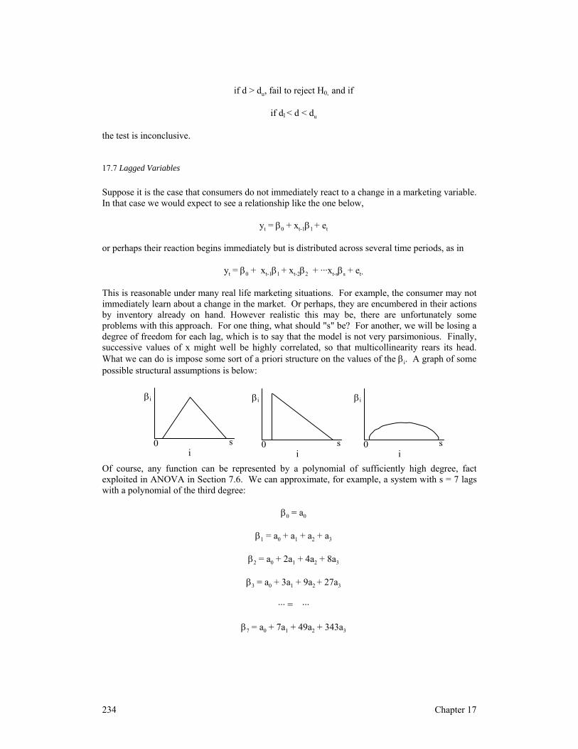
234 Chapter 17
if d > du, fail to reject H0, and if if dl < d < du the test is inconclusive.
17.7 Lagged Variables Suppose it is the case that consumers do not immediately react to a change in a marketing variable. In that case we would expect to see a relationship like the one below, yt = β0 + xt-1β1 + et or perhaps their reaction begins immediately but is distributed across several time periods, as in yt = β0 + xt-1β1 + xt-2β2 + ···xt-sβs + et. This is reasonable under many real life marketing situations. For example, the consumer may not immediately learn about a change in the market. Or perhaps, they are encumbered in their actions by inventory already on hand. However realistic this may be, there are unfortunately some problems with this approach. For one thing, what should "s" be? For another, we will be losing a degree of freedom for each lag, which is to say that the model is not very parsimonious. Finally, successive values of x might well be highly correlated, so that multicollinearity rears its head. What we can do is impose some sort of a priori structure on the values of the βi. A graph of some possible structural assumptions is below:
Of course, any function can be represented by a polynomial of sufficiently high degree, fact exploited in ANOVA in Section 7.6. We can approximate, for example, a system with s = 7 lags with a polynomial of the third degree: β0 = a0 β1 = a0 + a1 + a2 + a3 β2 = a0 + 2a1 + 4a2 + 8a3 β3 = a0 + 3a1 + 9a2 + 27a3 ··· = ··· β7 = a0 + 7a1 + 49a2 + 343a3
βi
i 0 s
βi
i 0 s
βi
i 0 s

Econometrics 235
The reader will perhaps recognize that the coefficients for the a values are constant in the first column, linear in the second, quadratic in the third and cubic in the fourth. If we substitute these equations back into the model for s = 7, i. e. yt = β0 + xt-1β1 + xt-2β2 + ···xt-7β7 + et, we get after collecting the ai terms yt = β0+ (xt + xt-1 + xt-2 + ··· x t-7)a0 + (xt + 2xt-1 + 3xt-2 + ··· + 7x t-7)a1 + (xt + 4xt-1 + 9xt-2 + ··· + 49x t-7)a2 + (xt + 8xt-1 + 27xt-2 + ··· + 343x t-7)a3 + et (17.17) which is equivalent to an model with yt = β0+ w0a0 + w1a1 + w2a2 + w3a3 + et, (17.18) where w0 = xt + xt-1 + xt-2 + ··· x t-7, and the other w values are defined as above in Equation (17.17). This is known as Almon's Scheme. If we define
⎥⎥⎥⎥⎥⎥
⎦
⎤
⎢⎢⎢⎢⎢⎢
⎣
⎡
=
3432771
842111110001
LLLL
K
using the coefficients for the x's, then KWWKβ ′′σ= −12 )()ˆ(V (17.19) lets you test the value s of the maximum lag, while 12 )()ˆ(V −′σ= WWa (17.20) lets you test the degree of the polynomial required to represent the lag structure. While Almon's Scheme is quite compelling, another approach was proposed by Koyck, who used a geometric sequence. Koyck started with the infinite sequence yt = xtβ0 + xt-1β1 + xt-2β2 + ··· + et. (17.21) Now, assume that the β values are all of the same sign, and that
.c0i
i ∞<=β∑∞
=
(17.22)
We now introduce the backshift operator, B, which is also prominently featured in Chapter 18. We define

236 Chapter 17
Bxt = xt-1. (17.23) Of course, one can also say BBxt = B
2xt = xt-2 (17.24)
and so forth with B
jxt = xt-j. Given our two assumptions of Equations (17.21) and (17.22), we can
rewrite the model as
t2t21t1t0
t22t11t0tt
e]xwxwxw[
exxxy
++++β=
++β+β+β=
−−
−−
L
L
where wi ≥ 0 for i = 0, 1, 2, ···, ∞ and .1w0i
i∑∞
=
= Given that, we can now rewrite the above
equation as .ex]BwBww[ tt
2210 ++++β= L
Now we introduce the major assumption of the Koyck scheme. The w's have a geometric relationship to each other as in wi = (1 - λ)λ
i (17.25)
where 0 < λ < 1. In that case
.B1
1)1(
)BB1)(1(BwBww 222210
λ−λ−=
+λ+λ+λ−=+++ LL
The fraction on the right hand side of the line immediately above is a consequence of the logic worked out in Equation (17.11) where we previously worked out the solution to an infinite series just like the one above. The upshot is that we can now write the model
)ee(yx)1(y
Bee)x-(1Byy
e)B1()x-(1y)B1(
exB1
)1(y
1tt1ttt
ttttt
ttt
ttt
−− λ−+λ+λ−β=
λ−+λβ=λ−
λ−+λβ=λ−
+λ−λ−β
=
(17.26)

Econometrics 237
As you can see, Koyck's scheme is characterized by autocorrelated error and lagged endogenous variables on the right hand side. Why would that be? Is there any marketing theory in which that would make sense? We will be finding out shortly.
17.8 Partial Adjustment by Consumers The partial adjustment model posits that the optimal value of the y variable, y*, might depend on x. For example, y could be an amount spent on our brand and x is income. As the consumer wants to make an optimal choice, and if the relationship is linear, we would have ,xy~ 1t0t β+β= (17.27) but due to less than perfect information about the market, inventory considerations, inertia, or the cognitive costs of change, the consumer can only adjust a certain proportion of the way from his or her previous value, yt-1, to the optimal value at .y~t In mathematical terms, t1tt1tt e)yy~(yy +−γ=− −− (17.28) with 0 < γ < 1. Substituting Equation (17.27) into Equation (17.28), we see that t1tt10t ey)1(xy +γ−+γβ+γβ= − which bears a resemblance to Koyck's scheme, only here we have an intercept, and the error is not autocorrelated.
17.9 Adaptive Adjustment by Consumers Another way that a similar equation may come about is through consumers adapting their expectations. Define tx~ as the expected level of x, and assume that some key consumer behavior depends on .x~ t The value tx~ could be the best guess of the price of a good, something to do with its availability in the market, and so forth. The consumer's behavior should then appear as below .ex~y t1t0t +β+β= (17.29) Now if we assume that the expectations are updated by a fraction of the discrepancy between the current observation and the previous expectation, we get
.xx~)1(x~
x~)1(x
x~x~xx~
)x~x(x~x~
t1tt
1tt
1t1ttt
1tt1tt
δ=δ−−
δ−+δ=
+δ−δ=
−δ=−
−
−
−−
−−
Define λ = 1 - δ. Then starting with the last line of the above equation,

238 Chapter 17
.xB1
x~
xx~)B1(
xx~x~
tt
tt
t1tt
λ−δ
=
δ=λ−
δ=λ− −
Finally, substituting this result into the model of Equation (17.29), we find out that
tt1
0
t1t0t
exB1
ex~y
+λ−
δβ+β=
+β+β=
which is the same as the Koyck Scheme of Equation (17.26). As far as estimating these models, OLS is not consistent [see Equation (5.11) for a definition of consistency] if there is autocorrelated error. You can use a two-stage estimator substituting 1ty − for yt-1. You can also use xt-1 as an instrument for yt-1.
17.10 Pooling Time Series and Cross Section Data Suppose we had for a particular sales region, call it region 1, the model )1()1()1()1( eβXy += where y
(1) is the T · 1 vector of observations on the response of the market in that region and X
(1) is
a matrix of marketing instruments including such factors as advertising effort, and so forth. In region 1 we might have k1 such instruments. Data have been collected from time period 1 through time period T and analogously, in region 2, we have done the same thing but with k2 different independent variables: .)2()2()2()2( eβXy += These two regression are only seemingly unrelated because we would expect 0)e,e(Cov )2(
t)1(
t ≠ as long as the two regions are interconnected economically. In point of fact, there are hardly two regions left on Earth that are not interconnected economically. The covariance identified above is called contemporaneous for obvious reasons. Alternating the regions so as to keep contemporaneous observations next to each other as we move from row to row, we could combine the two models as below:

Econometrics 239
⎥⎥⎥⎥⎥⎥⎥⎥⎥
⎦
⎤
⎢⎢⎢⎢⎢⎢⎢⎢⎢
⎣
⎡
+
⎥⎥⎥⎥⎥⎥⎥⎥⎥⎥⎥
⎦
⎤
⎢⎢⎢⎢⎢⎢⎢⎢⎢⎢⎢
⎣
⎡
β
βββ
ββ
⎥⎥⎥⎥⎥⎥⎥⎥⎥⎥
⎦
⎤
⎢⎢⎢⎢⎢⎢⎢⎢⎢⎢
⎣
⎡
=
⎥⎥⎥⎥⎥⎥⎥⎥⎥
⎦
⎤
⎢⎢⎢⎢⎢⎢⎢⎢⎢
⎣
⎡
)2(T
)1(T
)2(2
)1(2
)2(1
)1(1
)2(k
)2(1
)2(0
)1(k
)1(1
)1(0
)2(Tk
)2(1T
)1(Tk
)1(1T
)2(k2
)2(21
)1(k2
)1(21
)2(k1
)2(11
)1(k1
)1(11
)2(T
)1(T
)2(2
)1(2
)2(1
)1(1
ee
eeee
xx1000000xx1
xx1000000xx1
xx1000000xx1
yy
yyyy
2
1
2
1
2
1
2
1
L
L
L
LL
LL
LLLLLLLL
LL
LL
LL
LL
L
so that our model is now simply y = Xβ + e, with y having n times T rows, assuming n regions and T observations across time. For now we will continue to assume that n = 2. With contemporaneous covariance we can model the error covariance matrix as
nnTT
0
)(V Σ⊗=
⎥⎥⎥⎥
⎦
⎤
⎢⎢⎢⎢
⎣
⎡
= I
Σ0
0Σ000Σ
e
L
LLLL
L
L
where each null matrix and each copy of Σ is 2 · 2, and the Kronecker product operator ⊗ is defined in Section 1.10 (and elaborated on in Section 8.6). In fact, we might note the similarity between this and the error structure for the Multivariate General Linear model in Equation (8.36) and Equation (8.37). The difference is that in the General Linear Model, all dependent variables have the same set of independent variables. In this case, the seemingly unrelated model, we will use GLS, in which the error matrix, usually notated V, will be I ⊗ Σ as you can see now yΣIXXΣIXβ 111 )(])([ˆ −−− ⊗′⊗′= (17.30) and .])([)ˆ(V 11 −−⊗′= XΣIXβ We can apply a two step procedure in which we use OLS and estimate S = ,Σ then we apply GLS using S as a substitute for Σ in Equation (17.30). One could also use Maximum Likelihood. Another way to deal with the pooling problem is to use dummy variables, as we did in Section 7.3 in Equation (7.5) in the context of the analysis of variance. Of course, one could also use effect or orthogonal coding. If we set up dummies for each time period and each region, this purges the dependent variable of all variance associated with regions and time. This is a somewhat drastic approach, since some of the variance of interest will get thrown out with the bath water. A less drastic approach is to treat time and cross-sections like a random effect in ANOVA. Suppose that our error term is composed of eij = αi + ϕt + εit with V(αi) = ,2
ασ V(ϕt) = 2ϕσ and V(εit) = .2
εσ Given that the data from each region are next to each other in the y and e vectors,

240 Chapter 17
nT
2ennTT
2nnTT
2 )()()(V I11II11e σ+′⊗σ+⊗′σ= ϕα and we can apply a first step ANOVA to estimate the random variances 2
ασ and 2ϕσ while in the
second step we use those estimates in GLS. Parks has proposed a model like Zellner's seemingly unrelated regressions but with autoregressive error, and De Silva has suggested a model with variance components for the cross sections but autoregression for the time component.
References Johnston, J. (1972) Econometric Methods, Second Edition. New York: McGraw-Hill. Theil, Henri (1971) Principles of Econometrics. New York: Wiley. Maddala, G. S. (1977) Econometrics. New York: McGraw-Hill.


242 Chapter 18
Chapter 18: Time Series
18.1 Stationary Data Series In this chapter we consider a series of observation taken from a single entity over time much as we assumed in Section 17.5. The entity generating the data might be a particular company, Web site, household, market, geographic region or anything else that maintains a fixed identity over time. Our observations look like y1 , y2, ···, yn with a joint density Pr(y1 , y2, ···, yn). When data are collected over time, there is a very important concept that is called stationarity and in fact the concept shows up in other places in this book, notably Equation (15.1). For our purposes, we define the stationarity of a time series as Pr(yt , yt+1, ···, yt+k) = Pr(yt+m , yt+m+1, ···, yt+m+k), (18.1) for all t, j and k. Given that, it must be the case also that for m = ±1, ±2, ··· Pr(yt) = Pr(yt+m) which then further implies that E(yt) = E(yt+m) and V(yt) = V(yt+m). Presumably under stationarity it is the case as well that Pr(yt , yt+1) = Pr(yt+m , yt+m+1) (18.2) which would then make obvious the notion that Cov(yt , yt+1) = Cov(yt+m , yt+m+1) = γ1. In general, since Pr(yt , yt+j) = Pr(yt+m , yt+m+j) (18.3) the following is implied Cov(yt , yt+j) = Cov(yt+m , yt+m+j) = γj. The parameter γj is known as the autocovariance at lag j. Putting all of these results together, we can say that
⎥⎥⎥⎥
⎦
⎤
⎢⎢⎢⎢
⎣
⎡
μ
μμ
==
⎥⎥⎥⎥
⎦
⎤
⎢⎢⎢⎢
⎣
⎡
LL)(E
y
yy
E
n
2
1
y
and

Time Series 243
⎥⎥⎥⎥
⎦
⎤
⎢⎢⎢⎢
⎣
⎡
γγγ
γγγγγγ
=
−−
−
−
02n1n
2n01
1n10
)(V
L
LLLL
L
L
y
Like all covariance matrices, V(y) is symmetric. If E(yt) does not depend on t, which it should not with a stationary series, then we would ordinarily expect to find the series in the neighborhood of µ. History tends to repeat itself, probabilistically. By the definition of covariance [Equation (4.7)]: γj = E[(yt - µ)(yt+j - µ)]. If γj > 0 we would expect that a higher than usual observation would be followed by another higher than usual observation. We can standardize the covariances by defining the autocorrelation,
.0
j
00
jj γ
γ=
γγ
γ=ρ
As usual, ρ0 = 1. The structure of the autocorrelations will greatly help us in understating the behavior of the series, y.
18.2 A Linear Model for Time Series The time series models that we will be covering are called discrete linear stochastic processes and are of the form yt = µ + et + ψ1 et-1 + ψ2 et-2 + ··· . (18.4) In effect, an observation within the series is conceptualized as being the result of a possibly linear combination of random inputs. The et values are assumed identically distributed with E(et) = 0 and V(et) = .2
eσ Further, we will assume that Cov(et, et+j) = 0 (18.5) for all j ≠ 0. These et values are independent inputs and are often called white noise. We also assume that
c0i
i =ψ∑∞
=
and that
ψ0= 1.

244 Chapter 18
Given the preceding long list of notation and assumptions, what is the expectation and variance of our data? As was pointed out before, it is still the case the E(yt) = µ since we can combine Equation (18.4) and the assumption that E(et) = 0. As for the variance of V(yt), V(yt) = E(yt - µ)
2
= E(µ + et + ψ1 et-1 + ψ2 et-2 + ··· - µ)
2 (18.6)
where the two µ's will just cancel. Squaring the remaining terms, we can collect them into two sets: )eee(E)y(V e
2t22
21t
21
2tt L+ψ+ψ+= −− + E(all cross terms).
We can quickly dispense of all the cross terms from Equation (18.6) because, by assumption [Equation (18.5)] the et are independent. Worrying just about the first part of the above equation, and noting that the expectation of a sum is equal to the sum of the expectation[Equation (4.4)], we can then say that
.)y(V0i
2i
2et ∑
∞
=
ψσ= (18.7)
Are you game for figuring out the covariance at lag j of two data points from the series? Here goes. We note that the covariance between yt and yt-j is E[(yt - µ)(yt-j - µ)]. Once again, all values of µ will cancel leaving us with γj = E[(et + ψ1 et-1 + ψ2 et-2 + ···) (et-j + ψ1 et-j-1 + ψ2 et-j-2 + ···)] ++ψψ+ψψ+ψ= −−+−−+− ])e()e()e[(E 2
2jt22j2
1jt11j2
jtj L E(all cross terms). In this case, E(all cross terms) refers to any term involving E(et , et-m) for m ≠ 0 and once again, with independent et all such covariances vanish. That leaves us with the very manageable Equation (18.8)
∑∞
+
++
ψψσ=
+ψψ+ψψ+ψσ=γ
ijii
2e
21j11jj2ej )( L
(18.8)
Neither the variance in Equation (18.7) nor the covariances in Equation (18.8) can exist unless the infinite sum in those two equations is equal to a finite value. That an infinite series can be finite is seen in the reasoning that runs between Equation (15.17) and (15.17). We will return to this concept momentarily, but first we will assume that ψi = φ
i, with |φ| < 1. Then
yt = µ + et + φet-1 φ
2et-2 + ··· .
It can be shown that

Time Series 245
φ−
=φ=ψ ∑∑∞
=
∞
= 11
0i
i
0ii .
That this is so can be seen by defining s = ,1 32
0i
i L+φ+φ+φ+=φ∑∞
=
and then multiplying by φ
so that φs - s = 1. Solving for s leads to the result, s = .11 φ− Combining this result with Equation (18.7), yt then has a variance of
2
2e
0 1 φ−σ
=γ
and from Equation (18.8), autocovariances of
2
j2e
j 1 φ−φσ
=γ .
Needless to say, this will only work for with |φ| < 1, as otherwise, the variance will blow up. If φ = 1 our model becomes yt = µ + et + et-1 + et-2 + ··· = µ + et-1 + et-2 + ··· + et = yt-1 + et and so forth, as we could now substitute for yt-1 above. Obviously, the variance of a series with φ = 1 blows up.
18.3 Moving Average Processes A moving average model is characterized by a finite number of non-zero values ψi with ψi = 0 for i > q. The model will then look like the following, yt = µ + et + ψ1 et-1 + ψ2 et-2 + ··· + ψq et-q. The tradition in this area calls for us to modify the notation somewhat and utilize θi = -ψi which then modifies the look of the model slightly to yt = µ + et - θ1 et-1 - θ2 et-2 - ··· - θq et-q. Such as model is often called a Moving Average (q) process, or MA(q) for short. As an example, consider the MA(1): yt = µ + et - θ1 et-1
which can also be written with the Backshift operator, symbolized with the letter B and presented also in Equation (17.23):

246 Chapter 18
yt = µ + (1 - θ1B)et, i. e. Bet = et-1, (18.9) B · (Bet) = B
2et = et-1 and (18.10)
B
0et = et. (18.11)
We will have much cause to use the backshift operator in this chapter. For now, it will be interesting to look at the autocovariances of the MA(1) model. These will be
).(
)]ee)(ee[(E
12e
2t11t1t1t1
θ−σ=
θ−θ−=γ −−−
OK, that’s a nice result. What about the autocovariance at lag 2?
.0
)]ee)(ee[(E 3t12t1t1t2
=
θ−θ−=γ −−−
Since none of the errors overlap with the same subscript, everything vanishes as the errors are assumed independent. Thus we note that for the MA(1),
.1jfor01jfor1
2e
j⎩⎨⎧
>=θσ−
=γ
We can plot the autocorrelation function, which plots the value of the autocorrelations at various lags, j. In the case of the MA(1), the theoretical pattern is unmistakable:
As we will see later in the chapter, the correlogram, as a diagram such as the one above is called, is an important mechanism to identify the underlying structure of a time series. For the sake of curiosity, it will be nice to look at a simulated MA(1) process with θ1 = -.9 and µ = 5. The model would be
1 2 3 4 5 6 ··· j
+1
-1

Time Series 247
yt = et + .9et-1 and ,12
e =σ ,81.1)1( 21
2e0 =θ+σ=γ ,9.)( 1
2e1 =θσ−=γ 5.011 =γγ=ρ and ρj = 0 for all j > 1. An
example of this MA(1) process, produced using a random number generator is shown below: If θ1 = +.9 so that ρ1 = -.5 the correlogram would appear as
with the spike heading off in the negative, rather than the positive direction. The plot of the time series would by more jagged, since a positive value of yt would tend to be associated with a negative value of yt-1. For an arbitrary value of q, an MA(q) process will have autocovariances
1 2 3 4 5 6 ··· j
+1
-1
0
5
10
t
0
5
10
t

248 Chapter 18
⎩⎨⎧
>=θθ++θθ+θ−σ−
=γ −+
.qjfor0q,,2,1jfor( qjq1j1j
2e
jLL
For example the MA(2) process will have a correlogram that has two spikes:
18.4 Autoregressive Processes Recall that any discrete linear stochastic process can be expressed as yt = µ + et + ψ1 et-1 + ψ2 et-2 + ··· as was Equation (18.4). Needless to say this implies that we can express the errors as et = yt - µ - ψ1 et-1 - ψ2 et-2 - ··· . Our assumption of stationarity requires that the same basic model that holds for et must hold true for et-1 which would then be et-1 = yt-1 - µ - ψ1 et-2 - ψ2 et-3 - ··· . If we substitute the model for et-1 into the model for yt we get
L
LL
+ψ−ψ+ψ++ψ−μ=
+ψ+−ψ−μ−ψ++μ=
−−
−−−
2t2121t1t1
2t22t11t1tt
e)(ye)1(
e]ey[ey
You can keep doing this - now we substitute an expression for et-2 and so forth until all the et terms are banished and all that remains are yt values, with various coefficients. Arbitrarily naming these coefficients with the letter π, we get something that looks like yt = π1y t-1 + π2yt-2 + ··· + δ + et. (18.12) Our discrete linear stochastic process can be expressed as a possibly infinite series of past random disturbances [i. e. Equation (18.4)]. If the series is finite, we call it an MA process. Any discrete linear stochastic process can also be expressed as a possibly infinite series of its own past values disturbances [i. e. Equation (18.12)]. If the series is finite, we will call it an autoregressive
1 2 3 4 5 6 ···j
+1
-1

Time Series 249
process, also known as an AR process. This is illustrated below, where we have modified Equation (18.12) by assuming that πi = 0 for i > p: yt = φ1 yt-1 + φ2y t-2 + ··· + φpy t-p + δ + et. To the paragraph above, I would add that a finite AR is equivalent to an infinite MA and a finite MA is equivalent to an infinite AR. Below we will prove the first of these two assertions. But before we do that, it should be noted that all of this gives the data analyst a lot of flexibility in creating a parsimonious model. The AR(1) model looks like yt = φ1 yt-1 + δ + et (18.13) (1 - φ1B)yt = δ + et (18.14) If we take Equation (18.13) and substitute the equivalent expression for yt-1, we have yt = φ1 [φ1 yt-2 + δ + et-1] + δ + et and then again yt = φ1 [φ1 ([φ1 yt-3 + δ + et-2) + δ + et-1] + δ + et and so on until we see that we end up with
L+φ+φ+φ++φ−δ
= −−− 3t312t
211t1t
1t eeee
1y
which is an infinite MA process. As claimed, an AR(1) leads to an infinite MA. What are the moments of an AR(1) process? We have
,1
)y(E1
t φ−δ
=
and1 2
1
2ej
1j φ−σ
φ=γ
.j1j φ=ρ For the AR(1), the autocorrelations decline exponentially. An idealized correlogram is shown below:

250 Chapter 18
The autocorrelations damp out slowly. Next we show a random realization of the AR(1) model yt = .8yt-1 + 6 + et: Another example is identical to the first, but the sign on φ2 is reversed. The correlogram appears below
and then we see a random realization of the series:
1 2 3 4 5 6 ···j
+1
-1
j
+1
-1
25
30
35
t
-5
0
5
10
t

Time Series 251
18.5 Details of the Algebra of the Backshift Operator One of the most beautiful aspects of time series analysis is the use of backshift notation. Say we have an AR(1) with parameter φ1. We can express the model as (1 - φ1B)yt = et + δ. Putting the model in reduced form we have .e)B1()B1(y t
11
11t
−− φ−+δφ−= But what does it mean to invert a function with "B" in it? It produces an infinite series. To see that, start with the basic fact that
.B1
1)B1(1
11 φ−
=φ− −
So far so good. However, the series
L+φ+φ+φ+=φ=∑∞
=
331
2211
0i
ii1 BBB1Bs
and the series L+φ+φ+φ=⋅φ 33
122
111 BBBsB differ by 1. Thus s - φ1B · s = 1 and therefore
.BBB1B
B11)B1(s
331
2211
0i
ii1
1
11
L+φ+φ+φ+=φ=
φ−=φ−=
∑∞
=
−
(18.15)
Stationarity, and the need to avoid infinities in the infinite sum, require that |φ1| < 1. (18.16)

252 Chapter 18
This is equivalent to saying that the root of that 1 - φ1B = 0 must lie outside the unit circle.
18.6 The AR(2) Process The AR(2) model is
tt2
21
t2t21t1t
t2t21t1t
ey)BB1(
eyyy
eyyy
+δ=φ−φ−
+δ=φ−φ−
+δ+φ+φ=
−−
−−
which is stationary if the roots of 1 - φ1B - φ2B
2 = 0
lie outside the unit circle, which is to say φ1 + φ2 < 1, (18.17) φ1 - φ2 < 1 and (18.18) |φ2| < 1. (18.19) Below, the graph shows the permissible region as a shaded triangle:
18.7 The General AR(p) Process In general, an AR model of order p can be expressed as
φ1
0 -2
0
2
1
-1
φ2

Time Series 253
.)B(
ey
ey)B(
ey)BBB1(
tt
tt
ttp
p2
21
φ+δ
=
+δ=φ
+δ=φ−φ−φ−
Note that here we have introduced a new way of writing 1 - φ1B - φ2B
2 - ··· - φpB
p, namely to call it
simply φ(B). The autocorrelations and the φi are related to each other via what are known as the Yule-Walker Equations:
p2p21p1p
2pp2112
1pp1211
φ+ρφ+ρφ=ρ
=
ρφ+φ+ρφ=ρ
ρφ+ρφ+φ=ρ
−−
−
−
L
LL
L
L
which can be used to estimate jφ values.
18.8 The ARMA(1,1) Mixed Process Consider the model
.e)B1(y)B1(
eeyy
t1t1
1t1t1t1t
θ−+δ=φ−
θ−+φ+δ= −−
Here we have both an autoregressive and a moving average component. The AR part results in an infinite MA model with
.eB1B1
B1y t
1
1
1t φ−
θ−+
φ−δ
=
In compact notation we can say that ψ(B) = φ
-1(B) · θ(B). The MA part results in an infinite AR
model with
.eB1
yB1B1
t1
t1
1 =θ−δ
−θ−φ−

254 Chapter 18
Again we can compactify the notation noting that π(B) = φ(B) · θ-1(B). Mixed models let you
achieve parsimony as you can represent an infinite MA with a finite AR and vice versa. The situation that we have at hand can be graphed as follows:
We conceptualize of our observed series of data as being driven by are series of random shocks, of random values or white noise inputs. These inputs are then passed through a filter with various properties and that eventually leads to an output, which consists of our data. Modeling the data requires that we come up with a parsimonious description, one with few model parameters, of the filter, i.e ψ(B). What stationarity is to the AR side, invertibility is to the MA side. Invertibility requires that the roots of 1 - θ1B - θ2B
2 - ··· - θqB
q = 0
lie outside of the unit circle.
18.9 The ARIMA(1,1,1) Model A series may be relatively homogeneous, looking pretty much the same at all time periods, but it may end up being non-stationary simply because it shows no permanent affinity for a particular level or mean. Even though the original series of data may not be stationary, differences between successive observations may be stationary: dt = yt - yt-1 = (1 - B)yt. Simply put, we can apply an ARMA model to the dt. When we do so, this is called an ARIMA model with the middle I referring to the fact that it is integrated. If the first differences are not stationary, the second differences might be, i. e. d′t = dt - dt-1 = (1 - B)(1 - B)yt. The ARIMA(1,1,1) process, with the middle number referring to the number of differences that are taken can be described as
.eeyy)1(y
ee)yy(yy
eedd
t1t12t11t1t
t1t1tt11tt
t1t11t1t
+θ−φ−φ+=
+θ−−φ=−
+θ−φ=
−−−
−−−
−−
Thus we see that the ARIMA(1,1,1) is an ARMA(2,1) where the first ARMA AR parameter is equal to 1 + φ1 while the second ARMA(2,1) AR parameter is -φ1. These parameters violate the rules for stationarity in Equations (18.17), (18.18) and (18.19). Similarly, an ARIMA(0,1,1) process looks like
ψ(B)et yt

Time Series 255
yt = yt-1 + et - θ1et-1 which violates the stationarity rule for an AR(1) [Equation (18.16)] right off the top since "φ1" = 1! Thus we see the importance of differencing the series first, if necessary, prior to fitting an ARMA model. We can wrap up this section with another brief note about the backshift notation and the ARIMA(1,1,1) model. Such a model can be written quite elegantly as (1 - φ1B)(1 - B)yt = δ + (1 - θ1B)et
In the model, the constant term δ implies that the average change will have the same sign as δ and the series will drift in the direction of the sign of δ.
18.10 Seasonality Differencing, AR or MA parameters may be needed at various lags. For quarterly data, you may need to look at lags of 4, or for monthly data, lags of 12, which may occur whenever there are yearly patterns in data. For example, the following pattern seen in quarterly data:
may require that you difference the data at a lag of 4, i.e analyze dt = (1 - B
4)y
t.
18.11 Identifying ARIMA(p,d,q) Models In addition to the cues afforded in the autocorrelations, we can also look at what are known as the partial autocorrelations. For each lag j, you estimate ρj controlling for the first j - 1 values ρj-1, ρj-2, ···, ρ1. For a nonstationary process, the autocorrelations will be large at very long lags. On the other hand, over-differencing tends to produce an MA(1) with θ1 = 1. For an AR process, the autocorrelations will decline exponentially. The partial autocorrelations will exhibit significant spikes at the first p lags. For an MA process, the autocorrelations will exhibit significant spikes at the first q lags. The partial autocorrelations will exhibit exponential decline.
j
+1
-1

256 Chapter 18
For a mixed process, the autocorrelations as well as the partial autocorrelations will decline exponentially. It is generally a good idea to run the error of your model through the same diagnostic process to make sure that it is indeed acting like white noise. In effect, one adds a term to the ARIMA model, and then looks at the error to see if it is white noise yet. The process is repeated until the error is completely whitened.
References Box, George E. P., Gwilym M. Jenkins (1976) Time Series Analysis. Revised Edition. Oakland, CA: Holden-Day.

257
Appendices A. The Greek Alphabet alpha
beta
gamma
delta
epsilon
zeta
eta
theta
iota
kappa
lambda
mu
nu
xi or ksi
omicron
phi
rho
sigma
tau
upsilon
phi
chi
psi
omega
α
β
γ
δ
ε
ζ
η
θ
ι
κ
λ
μ
ν
ξ
ο
π
ρ
σ
τ
υ
φ
χ
ψ
ω
Α
Β
Γ
Δ
Ε
Ζ
Η
Θ
Ι
Κ
Λ
Μ
Ν
Ξ
Ο
Π
Ρ
Σ
Τ
Υ
Φ
Χ
Ψ
Ω

258
Index τ-equivalent tests.............................................118 2SLS ...............................................................225 a priori.............................................66, 67, 72, 86 absolute threshold ...........................................146 additive conjoint measurement ......................190 aggregate data .................................................168 algebra for matrices .........................................3 all y models ...................................................127 Almon's scheme ..............................................235 ALS.................................................................191 alternating least squares ..........................191, 193 alternative specific constants...........................182 alternative specific variables ...........................182 analytical solution .............................................31 angle-preserving transformation .......................30 ANOVA ..........................................................76 AR...................................................................249 arithmetic mean...............................................See ASC ................................................................182 associative property of matrix addition ...............6 associative property of scalar multiplication.......4 ASV ................................................................182 asymptotic efficiency ........................................34 attraction .........................................................168 autocovariance ................................................242 autoregression .................................................248 autoregressive process.....................................249 backshift operator............................235, 245, 251 beta distribution ..............................................206 big R squared ....................................................70 bilinear form .......................................................8 brand switching...............................................204 canonical correlation .....................................99 category rating scale .......................................157 central limit theorem ........................................64 chain rule ..........................................................22 Chi Square.......................................................41 city block metric. ............................................195 classification .................................................104 closed form solution..........................................31 Cobb-Douglas function ...................................221 Cochrane-Orcutt iterative procedure ...............233 Cochran's theorem .........................................43 coding
dummy..........................................................78 effect.............................................................77 orthogonal.....................................................79
column centering...............................................16 column vector ...................................... See vector common factors.......................................111, 137 communalities.........................................137, 138 communality ...................................................137 commutative property of matrix addition............6 comparative judgment model ..........................182 conditional logit ......................................182, 183
conditional probability ............................105, 205 confidence interval ........................................... 66 confidence intervals ....................................... 66 conformable for addition.................................... 4 congeneric tests .............................................. 118 congeneric tests. ............................................. 118 conjoint ......................................................... 190 constant elasticity model ................................ 222 contemporaneous correlation ......................... 238 correct rejection.............................................. 160 corrected SSCP matrix ..................................... 16 corrected sum of square and cross products ..... 16 correlation, squared multiple............................ 70 correlogram .................................................... 246 covariance ........................................................ 14 covariance structure models ........................... 110 cross effects.................................................... 183 cross product .................................................... 15 crossing ............................................................ 84 cross-product matrix.......................................... 9 cross-products ................................................ 96 cumulated probabilities .................................. 158 density function.......................................... 36, 37 derivative
scalar............................................................ 20 trace ............................................................ 89 vector ........................................................... 23
derivative of a scalar with respect to a vector... 22 derivative of a sum ........................................... 21 derivative of the transpose................................ 23 determinant....................................................... 11 determinant of a matrix................................. 11 deviation score ................................................. 14 Diag function.................................................... 17 diagonal............................................................ 18 diagonal matrix................................................... 5 dichotomous dependent variable .................... 168 difference thresholds ...................................... 147 differential effects .......................................... 183 direct product ................................................... 90 disaggregate data............................................ 169 discrete choice................................................ 168 discriminal process......................................... 151 discriminant function...............................104, 107 distances ......................................................... 194 distribution
beta hat......................................................... 64 chi square..................................................... 41 F 45 multivariate normal...................................... 40 Student's t..................................................... 43
distribution function ......................................... 37 distribution function, normal............................ 39 distributive property of scalar multiplication ..... 5 dot product ......................................................... 6

259
dummy coding ..................................................78 Dunn-Bonferroni.........................................86, 99 effect coding .....................................................77 efficiency ........................................................170 eigenstructure....................................24, 91, 137 eigenvalue .........................................................26 eigenvector........................................................26 eigenvectors
left ................................................................92 right ..............................................................92
elasticity ..................................................184, 220 endogenous variables ......................................124 equimax...........................................................143 error term ..........................................................84 error transform ..................................................74 error, specification ..................................111, 124 error-in-equations............................................111 errors-in-equations ..........................................124 errors-in-variables ...........................................111 estimation ....................................30, 48, 52, 153 estimator ..........................................................93 euclidean distance ...........................................193 exogenous variables ........................................124 expectation ........................................................36 expectation of a random variable ......................36 exponential distribution...................................214 exponents ..........................................................20 external unfolding ...........................................201 extraction
factor...........................................................140 F distribution.............................................45, 69 factor
rotation .......................................................140 factor extraction............................................140 factor loadings.................................................111 factor structure ................................................143 factors .............................................................110 false alarm.......................................................160 false alarm rate................................................162 FAR ........................................................160, 162 Fechner’s law..................................................146 full information maximum likelihood .............225 full rank.............................................................28 fully extended model.......................................183 fundamental theorem of market share .....181, 182 Fundamental theorem of market share ............185 Gauss-Markov assumption........................52, 230 generalized least squares...........................72, 175 generalized Minkowski metric ........................195 generic variable...............................................182 GFI..................................................................120 global minimum........................................32, 117 GLS................................... 72, 175, 177, 182, 239 goodness of fit ..............................................120 goodness of fit index.......................................120 group space .....................................................196 Hessian..............................................................33 heterogeneity ................................................206
heteroskedasticity ....................................170, 171 hit 160 hit rate ............................................................ 162 Hotelling-Lawleys trace ................................... 98 HR...........................................................160, 162 hypotheses............................................66, 67, 68 ideal point model ......................................... 199 idempotency ..................................................... 74 identity element of matrix addition .................... 6 identity element of matrix multiplication ......... 11 identity matrix .................................................... 5 IIA.................................................................. 185 income type variable ...............................168, 181 index, goodness of fit ..................................... 120 INDSCAL ...............................................196, 201 information matrix ........................................... 34 initial state vector ........................................... 209 inner product ...................................................... 6 instrumental variables .................................... 227 interaction......................................................... 80 intercept-only ................................................. 58 internal unfolding ........................................... 201 inverse normal distribution function............... 153 inverse of a matrix................................... 12, 13 isopreference contours.............................198, 200 JND ................................................................ 147 joint probability.............................................. 205 joint space ...................................................... 199 just identified.................................................. 129 just noticeable difference................................ 147 Koyck's scheme.............................................. 235 Kronecker product......................................... 90 Lagrange multiplier .......................................... 25 latent variables ............................................... 110 law of categorical judgment ...................... 157 Law of comparative judgment .................. 150 law of total probability ................................... 210 learning models............................................ 211 least squares ..................................................... 49 least squares regression .................................... 48 left eigenvectors ............................................... 92 length of a vector................................................ 7 levels of variables............................................. 55 likelihood ....................................................... 208 linear algebra ................................................... 2 linear combination.............................................. 6 linearization.................................................... 173 ln 20 loadings .......................................................... 111 local minimum ......................................... 32, 117 log .................................................................... 20 logarithms....................................................... 20 Logarithms ..................................................... 20 logically inconsistent...................................... 170 logistic regression........................................... 171 logit .........................................................171, 173 logit χ2............................................................ 156

260
logit model ......................................................168 logit, conditional .............................................168 logit, polytomous ............................................168 loss function......................................................49 MA(q) .............................................................245 Mahalanobis distance......................................106 manifest variables ...........................................111 MANOVA ....................................................101 marginal probability........................................205 marketing instrument ......................................183 markov chains ...............................................209 matrices............................................................15
partitioned.......................................................8 matrix..................................................................2
cross-product ..................................................9 determinant ...................................................11 inverse ....................................................12, 13 multiplication................................................10 trace ........................................................11, 89
matrix addition....................................................4 matrix addition, associative property ..................6 matrix addition, commutative property ...............6 matrix addition, identity element ........................6 matrix algebra .....................................................3 matrix conditional ...........................................195 matrix multiplication........................................7 matrix multiplication, identity element .............11 matrix notation .................................................2 matrix subtraction ...............................................5 matrix transposition ............................................3 matrix, diagonal ..................................................5 matrix, identity....................................................5 matrix, null..........................................................5 matrix, postmultiplying.......................................7 matrix, premultiplication.....................................7 matrix, rank...............................................28, 137 matrix, scalar.......................................................5 matrix, unit..........................................................5 matrix, variance-covariance ..............................17 maximum likelihood..............................32, 156 Maximum Likelihood .......................................32 MCI.................................................................183 MDS................................................................192 mean................................................................See mean vector.......................................................15 measures, commensurate ..................................83 method of moments.........................................214 metric ..............................................................194 minimum Pearson χ2 ..............................154, 177 minimum, local ...............................................117 mispecified model...........................................111 miss .................................................................160 mixing distribution..........................................204 MNL ...............................................................180 MNL model.............................................180, 182 MNL, simple effects .......................................183 modes..............................................................195 modification index ..........................................121
modified minimum χ2 .............................156, 177 moving average............................................ 245 moving average (q) process............................ 245 multidimensional scaling............................ 192 multi-method multi-trait.............................. 118 multinomal logit model .................................. 180 multiplication, vector ......................................... 6 multiplicative competitive interaction ............ 183 multivariate normal distribution .................. 40 n-afc procedure............................................... 163 NBD ............................................................... 213 negative binomial........................................ 215 negative binomial distribution........................ 213 nesting .............................................................. 84 NIID ................................................................. 52 non-linear optimization .................................... 31 nonmetric MDS.............................................. 192 non-recursive.................................................. 130 nonrecursive systems .................................. 224 normal distribution ........................................ 37 normal distribution function............................. 39 normal equations .............................................. 50 null matrix .......................................................... 5 of commensurate variables............................... 83 off-diagonal ........................................................ 5 ogive......................................................... 39, 172 one-way analysis of variance ........................... 76 operator, error.........................See error transform operator, expectation ........................................ 36 operator, prediction ....... See prediction transform operator, variance............................................. 37 optimal scaling ............................................... 191 order of a matrix................................................. 2 ordinary least squares ....................................... 48 orthogonal .......................................................... 6 orthogonal coding............................................ 79 orthonormal...................................................... 29 outer product ...................................................... 8 paired comparisons......................................... 151 parallel tests.................................................... 118 parameter estimation................................. 30, 32 partial autocorrelations................................... 255 partial derivative............................................... 22 partitioned matrices ......................................... 8 part-worths ..................................................... 192 perception ..................................................... 195 perceptual space ............................................. 193 Pillai's trace ...................................................... 98 Plim.................................................................. 51 polychoric correlation .................................... 159 polytomous dependent variable...................... 168 posterior probability ....................................... 208 postmultiplying matrix ....................................... 7 prediction transform ......................................... 74 preference vector ............................................ 198 premultiplying matrix......................................... 7 price elasticity of market share....................... 184

261
price type variable...................................168, 182 pricing............................................................222 principal axis.....................................................25 prior distribution .............................................208 prior probability ..............................................105 probability
law of total..................................................210 probit...............................................................171 probit model............................................171, 186 projections.......................................................198 proximity judgments .......................................193 purchase incidence .......................................213 quadratic equation.............................................27 quadratic form.....................................................8 qualitative independent variables ......................76 quantitative independent variables...............82 quartimax ........................................................143 rank of a matrix...............................................137 rank of a square matrix......................................28 rank, full............................................................28 ratings procedure.............................................161 rational consumer............................................168 raw cross products matrix .................................16 receiver operating characteristic......................162 recursive system..............................................130 reduced form...................................................125 regression..........................................................48 repeated measures ..................................83, 101 response bias ...................................................159 right eigenvectors..............................................92 rigid transformation ..........................................30 ROC ........................................................162, 163 root mean square error ....................................121 rotation ...........................................................140 row vector ............................................ See vector Roy's largest root ..............................................98 RUM ...............................................................168 scalar ...................................................................2 scalar derivative ................................................20 scalar function of a vector.............................22 scalar matrix........................................................5 scalar multiplication............................................4 scalar multiplication, distributive property .........5 scalar multiplication,associative property ...........4 scalar product ......................................................6 scaling, optimal ...............................................191 scree chart .......................................................138 seasonality.....................................................255 second order
derivative ......................................................23 second order derivative .....................................23 seemingly unrelated regression .......................238 setting a metric ...............................................114 Shepard diagram .............................................191 similarity judgment .........................................195 similarity judgments........................................193 simple effects MNL ........................................183 simple effects model .......................................182
simple structure .............................................. 142 singular value decomposition........................... 92 SMC ................................................................. 70 specification error........................................... 111 specification errors ......................................... 124 spike ............................................................... 248 square matrix...................................................... 3 squared multiple correlation............................. 70 SS predictable .................................................. 54 SS Total............................................................ 54 SSCP matrix ..................................................... 16 SSCP matrix, corrected .................................... 16 SSCP, raw ........................................................ 16 SSE................................................................... 54 SSErro ................................................................ 54 standard deviation ............................................ 14 standardized scores........................................... 14 starting values .................................................. 31 stationarity...................................................... 242 stationary........................................................ 204 stress........................................................191, 193 Student's t-statistic......................................... 43 subscript reduction operator ............................... 3 sum constrained.............................................. 170 sum of square and cross products, corrected .... 16 sum of squares.................................................. 14 sum of squares and cross products ................... 93 sum of squares and cross products, raw ........... 16 sum of squares and cross products, uncorrected16 sum of squares error ......................................... 54 sum of squares predictable ............................... 54 sum of squares total.......................................... 54 sums of squares.............................................. 54 superior-inferior model .................................. 211 supremum metric............................................ 195 symmetric matrix ............................................... 4 t distribution ..................................................... 43 theory of signal detectability...............159, 164 three way data ................................................ 195 Thurstone model......................................171, 182 Thurstone’s law.............................................. 168 trace of a matrix ....................................... 11, 89 transformation, angle-preserving...................... 30 transformation, rigid......................................... 30 transition matrix ..............................206, 209, 211 transpose operator .............................................. 2 transpose, derivative......................................... 23 treatments ......................................................... 76 triangle inequality........................................... 195 t-statistic.......................................................... 43 two way data .................................................. 195 type I error........................................................ 67 uncorrected SSCP............................................. 16 uncorrected sum of squares and cross products 16 unfolding ........................................................ 200 unfolding, external ......................................... 201 unfolding, internal .......................................... 201 union-intersection............................................. 99

262
union-Intersection ..........................................88 unique factors..................................................111 unit matrix...........................................................5 univariate statistics ........................................14 universal logit model.......................................183 unobserved variables.......................................110 unweighted least squares.................................173 utilities ....................................................151, 192 utility...............................................................168 variables, commensurate...................................83 variance.............................................................14 variance matrix .................................................17 variance operator...............................................37 variance-covariance matrix ...............................17 variances..........................................................36 variety-seeking model .....................................211 varimax procedure ..........................................142
vec.................................................................... 91 vector.................................................................. 2
scalar function of a....................................... 22 vector derivative ............................................. 23 vector model ................................................. 197 vector multiplication .......................................... 6 vector notation ................................................. 2 vector outer product ........................................... 8 vector, length...................................................... 7 weighted euclidean model .............................. 196 weighted least squares.............................. 72, 173 weighted nonlinear least squares .............154, 155 white noise ..............................................231, 243 Wilk's lambda................................................... 98 WLS ................................................................. 72 yes/no task...................................................... 159 Yule-Walker equations................................... 253


![Background Methods Results & ConclusionsMethods Design [quant → QUAL] Quant Data Collection. Phase 1: Quant. Phase 2: QUAL . Quant Data Analysis. QUAL Data Analysis . Integration](https://static.fdocuments.in/doc/165x107/6000faa49b2cd844807c19b1/background-methods-results-conclusions-methods-design-quant-a-qual-quant.jpg)