
Quality Management Class 4: 2/9/11. Total Quality Management Defined Quality Specifications and...
63
Quality Management Class 4: 2/9/11
-
Upload
mitchell-boone -
Category
Documents
-
view
221 -
download
1
Transcript of Quality Management Class 4: 2/9/11. Total Quality Management Defined Quality Specifications and...

Quality Management
Class 4: 2/9/11
Total Quality Management Defined
Quality Specifications and Costs Six Sigma Quality and Tools External Benchmarking ISO 9000 Service Quality Measurement Process Variation Process Capability Process Control Procedures
OBJECTIVES

TOTAL QUALITY MANAGEMENT (TQM)
Total quality management is defined as managing the entire organization so that it excels on all dimensions of products and services that are important to the customerCareful design of product or serviceEnsuring that the organization’s
systems can consistently produce the design
TQM was a response to the Japanese superiority in quality

QUALITY SPECIFICATIONS
Design quality: Inherent value of the product in the marketplace
Dimensions include: Performance, Features, Reliability/Durability, Serviceability, Aesthetics, and Perceived Quality.
Conformance quality: Degree to which the product or service design specifications are met

Crosby: conformance to requirementsDeming: A predictable degree of
uniformity and dependability at low cost and suited to the market
Juran: fitness for use (satisfies customer’s needs)
Three Quality Gurus Define Quality

Create consistency of purpose Lead to promote change Build quality into the products Build long term relationships Continuously improve product, quality, and
service Start training Emphasize leadership
Deming’s 14 Points
Drive out fear Break down barriers between departments Stop haranguing workers Support, help, improve Remove barriers to pride in work Institute a vigorous program of education and
self-improvement Put everybody in the company to work on the
transformation
Deming’s 14 Points

4.Act 1.Plan
3.Check 2.Do
Identify the improvement and make a plan
Test the planIs the plan working
Implement the plan
Shewhart’s PDCA Model
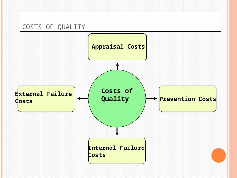
COSTS OF QUALITY
External Failure Costs
Appraisal Costs
Prevention Costs
Internal FailureCosts
Costs ofQuality

SIX SIGMA QUALITY
A philosophy and set of methods companies use to eliminate defects in their products and processes
Seeks to reduce variation in the processes that lead to product defects

SIX SIGMA QUALITY (CONTINUED)
Six Sigma allows managers to readily describe process performance using a common metric: Defects Per Million Opportunities (DPMO)
1,000,000 x
units of No. x
unit per error for
iesopportunit ofNumber
defects ofNumber
DPMO 1,000,000 x
units of No. x
unit per error for
iesopportunit ofNumber
defects ofNumber
DPMO

SIX SIGMA QUALITY (CONTINUED)
Example of Defects Per Million Opportunities (DPMO) calculation. Suppose we observe 200 letters delivered incorrectly to the wrong addresses in a small city during a single day when a total of 200,000 letters were delivered. What is the DPMO in this situation?
Example of Defects Per Million Opportunities (DPMO) calculation. Suppose we observe 200 letters delivered incorrectly to the wrong addresses in a small city during a single day when a total of 200,000 letters were delivered. What is the DPMO in this situation?
000,1 1,000,000 x
200,000 x 1
200DPMO
000,1 1,000,000 x
200,000 x 1
200DPMO
So, for every one million letters delivered this city’s postal managers can expect to have 1,000 letters incorrectly sent to the wrong address.
So, for every one million letters delivered this city’s postal managers can expect to have 1,000 letters incorrectly sent to the wrong address.
Cost of Quality: What might that DPMO mean in terms of over-time employment to correct the errors?
Cost of Quality: What might that DPMO mean in terms of over-time employment to correct the errors?

SIX SIGMA QUALITY: DMAIC CYCLE
Define, Measure, Analyze, Improve, and Control (DMAIC)
Developed by General Electric as a means of focusing effort on quality using a methodological approach
Overall focus of the methodology is to understand and achieve what the customer wants
A 6-sigma program seeks to reduce the variation in the processes that lead to these defects
DMAIC consists of five steps….

SIX SIGMA QUALITY: DMAIC CYCLE (CONTINUED)
1. Define (D)
2. Measure (M)
3. Analyze (A)
4. Improve (I)
5. Control (C)
Customers and their priorities
Process and its performance
Causes of defects
Remove causes of defects
Maintain quality

EXAMPLE TO ILLUSTRATE THE PROCESS… We are the maker of this cereal. Consumer
reports has just published an article that shows that we frequently have less than 16 ounces of cereal in a box.
What should we do?
STEP 1 - DEFINE
What is the critical-to-quality characteristic? The CTQ (critical-to-quality) characteristic in
this case is the weight of the cereal in the box.

2 - MEASURE
How would we measure to evaluate the extent of the problem?
What are acceptable limits on this measure?

2 – MEASURE (CONTINUED)
Let’s assume that the government says that we must be within ± 5 percent of the weight advertised on the box.
Upper Tolerance Limit = 16 + .05(16) = 16.8 ounces
Lower Tolerance Limit = 16 – .05(16) = 15.2 ounces
2 – MEASURE (CONTINUED)
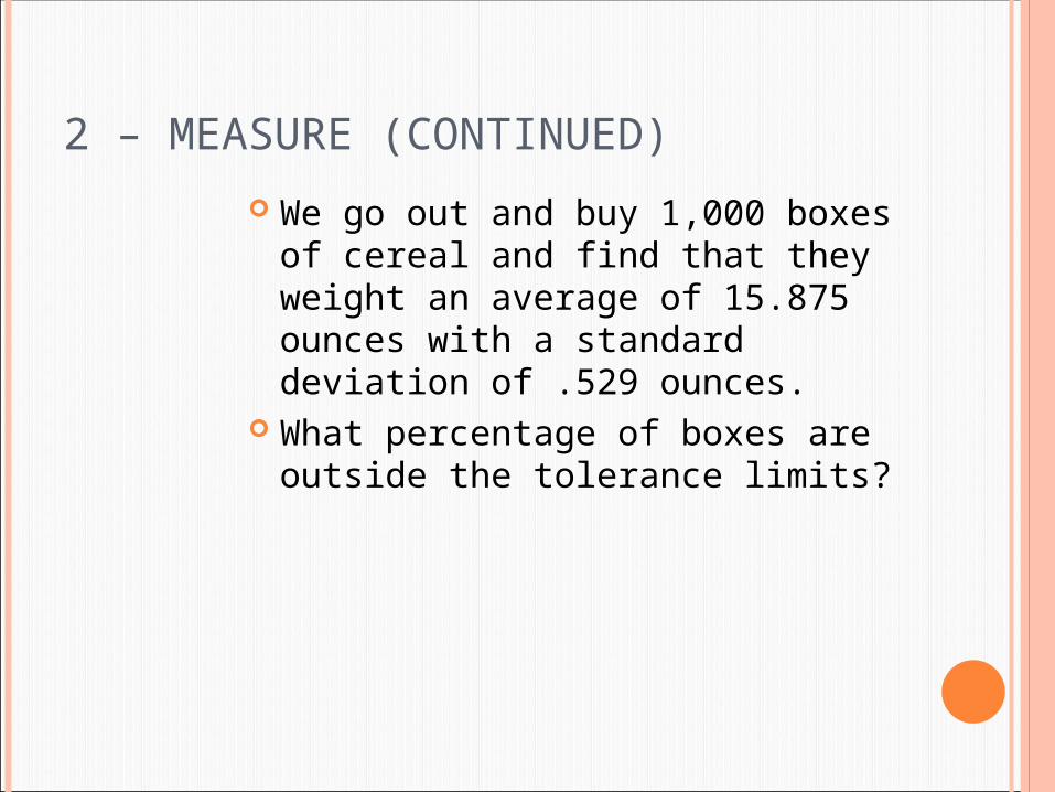
We go out and buy 1,000 boxes of cereal and find that they weight an average of 15.875 ounces with a standard deviation of .529 ounces.
What percentage of boxes are outside the tolerance limits?

Upper Tolerance = 16.8
Lower Tolerance = 15.2
ProcessMean = 15.875Std. Dev. = .529
What percentage of boxes are defective (i.e. less than 15.2 oz)?
Z = (x – Mean)/Std. Dev. = (15.2 – 15.875)/.529 = -1.276
NORMSDIST(Z) = NORMSDIST(-1.276) = .100978
Approximately, 10 percent of the boxes have less than 15.2 Ounces of cereal in them!

STEP 3 - ANALYZE - HOW CAN WE IMPROVE THE CAPABILITY OF OUR CEREAL BOX FILLING PROCESS?
Decrease VariationCenter ProcessIncrease Specifications

STEP 4 – IMPROVE – HOW GOOD IS GOOD ENOUGH? MOTOROLA’S “SIX SIGMA”
6 minimum from process center to nearest spec
1 23 1 02 3
12
6

MOTOROLA’S “SIX SIGMA” Implies 2 ppB “bad” with no process shift. With 1.5 shift in either direction from center (process
will move), implies 3.4 ppm “bad”.
1 23 1 02 3
12

STEP 5 – CONTROL
Statistical Process Control (SPC)Use data from the actual
processEstimate distributionsLook at capability - is good
quality possibleStatistically monitor the
process over time

ANALYTICAL TOOLS FOR SIX SIGMA AND CONTINUOUS
IMPROVEMENT: FLOW CHART
No, Continue…
Material Received from Supplier
Inspect Material for Defects
Defects found?
Return to Supplier for Credit
Yes
Can be used to find quality problems
Can be used to find quality problems

ANALYTICAL TOOLS FOR SIX SIGMA AND CONTINUOUS IMPROVEMENT: RUN CHART
Can be used to identify when equipment or processes are not behaving according to specifications
Can be used to identify when equipment or processes are not behaving according to specifications
0.440.460.480.5
0.520.540.560.58
1 2 3 4 5 6 7 8 9 10 11 12Time (Hours)
Dia
me
ter

ANALYTICAL TOOLS FOR SIX SIGMA AND CONTINUOUS IMPROVEMENT: PARETO ANALYSIS
Can be used to find when 80% of the problems may be attributed to 20% of thecauses
Can be used to find when 80% of the problems may be attributed to 20% of thecauses
Assy.Instruct.
Fre
quen
cy
Design Purch. Training
80%

ANALYTICAL TOOLS FOR SIX SIGMA AND CONTINUOUS IMPROVEMENT: CHECKSHEET
Billing Errors
Wrong Account
Wrong Amount
A/R Errors
Wrong Account
Wrong Amount
Monday
Can be used to keep track of defects or used to make sure people collect data in a correct manner
Can be used to keep track of defects or used to make sure people collect data in a correct manner

ANALYTICAL TOOLS FOR SIX SIGMA AND CONTINUOUS IMPROVEMENT: HISTOGRAM
Nu
mb
er
of
Lo
ts
Data RangesDefectsin lot
0 1 2 3 4
Can be used to identify the frequency of quality defect occurrence and display quality performance
Can be used to identify the frequency of quality defect occurrence and display quality performance

ANALYTICAL TOOLS FOR SIX SIGMA AND CONTINUOUS IMPROVEMENT: CAUSE & EFFECT DIAGRAM
Effect
ManMachine
MaterialMethod
Environment
Possible causes:Possible causes: The results or effect
The results or effect
Can be used to systematically track backwards to find a possible cause of a quality problem (or effect)
Can be used to systematically track backwards to find a possible cause of a quality problem (or effect)

ANALYTICAL TOOLS FOR SIX SIGMA AND CONTINUOUS IMPROVEMENT: CONTROL CHARTS
Can be used to monitor ongoing production process quality and quality conformance to stated standards of quality
Can be used to monitor ongoing production process quality and quality conformance to stated standards of quality
970
980
990
1000
1010
1020
0 1 2 3 4 5 6 7 8 9 10 11 12 13 14 15
LCL
UCL

SIX SIGMA ROLES AND RESPONSIBILITIES
1. Executive leaders must champion the process of improvement
2. Corporation-wide training in Six Sigma concepts and tools
3. Setting stretch objectives for improvement
4. Continuous reinforcement and rewards

THE SHINGO SYSTEM: FAIL-SAFE DESIGN
Shingo’s argument:SQC methods do not prevent defectsDefects arise when people make
errorsDefects can be prevented by
providing workers with feedback on errors
Poka-Yoke includes:ChecklistsSpecial tooling that prevents
workers from making errors

ISO 9000 AND ISO 14000
Series of standards agreed upon by the International Organization for Standardization (ISO)
Adopted in 1987
More than 160 countries
A prerequisite for global competition?
ISO 9000 an international reference for quality, ISO 14000 is primarily concerned with environmental management
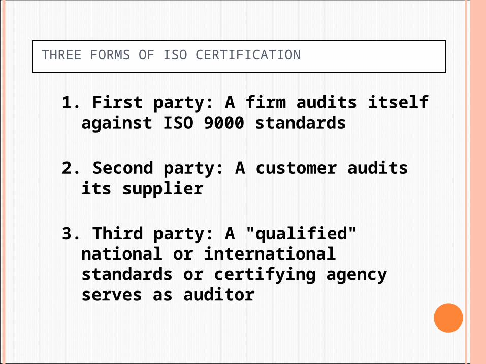
THREE FORMS OF ISO CERTIFICATION
1. First party: A firm audits itself against ISO 9000 standards
2. Second party: A customer audits its supplier
3. Third party: A "qualified" national or international standards or certifying agency serves as auditor

EXTERNAL BENCHMARKING STEPS
1. Identify those processes needing improvement
2. Identify a firm that is the world leader in performing the process
3. Contact the managers of that company and make a personal visit to interview managers and workers
4. Analyze data

Process Variation Process Capability Process Control Procedures
Variable data Attribute data
Process Control

BASIC FORMS OF VARIATION
Assignable variation is caused by factors that can be clearly identified and possibly managed
Common variation is inherent in the production process
Example: A poorly trained employee that creates variation in finished product output.
Example: A poorly trained employee that creates variation in finished product output.
Example: A molding process that always leaves “burrs” or flaws on a molded item.
Example: A molding process that always leaves “burrs” or flaws on a molded item.

TAGUCHI’S VIEW OF VARIATION
IncrementalCost of Variability
High
Zero
LowerSpec
TargetSpec
UpperSpec
Traditional View
IncrementalCost of Variability
High
Zero
LowerSpec
TargetSpec
UpperSpec
Taguchi’s View
Traditional view is that quality within the LS and US is good and that the cost of quality outside this range is constant, where Taguchi views costs as increasing as variability increases, so seek to achieve zero defects and that will truly minimize quality costs.
Traditional view is that quality within the LS and US is good and that the cost of quality outside this range is constant, where Taguchi views costs as increasing as variability increases, so seek to achieve zero defects and that will truly minimize quality costs.

PROCESS CAPABILITY
Process limits
Specification limits
How do the limits relate to one another?

PROCESS CAPABILITY INDEX, CPK
3
X-UTLor
3
LTLXmin=C pk
Shifts in Process Mean
Capability Index shows how well parts being produced fit into design limit specifications.
Capability Index shows how well parts being produced fit into design limit specifications.
As a production process produces items small shifts in equipment or systems can cause differences in production performance from differing samples.
As a production process produces items small shifts in equipment or systems can cause differences in production performance from differing samples.

A simple ratio: Specification Width
_________________________________________________________
Actual “Process Width”
Generally, the bigger the better.
PROCESS CAPABILITY – A STANDARD PROCESS CAPABILITY – A STANDARD MEASURE OF HOW GOOD A PROCESS IS.MEASURE OF HOW GOOD A PROCESS IS.

PROCESS CAPABILITYPROCESS CAPABILITY
This is a “one-sided” Capability IndexConcentration on the side which is closest to the
specification - closest to being “bad”
3
;3
XUTLLTLXMinC pk

THE CEREAL BOX EXAMPLE
We are the maker of this cereal. Consumer reports has just published an article that shows that we frequently have less than 16 ounces of cereal in a box.
Let’s assume that the government says that we must be within ± 5 percent of the weight advertised on the box.
Upper Tolerance Limit = 16 + .05(16) = 16.8 ounces
Lower Tolerance Limit = 16 – .05(16) = 15.2 ounces
We go out and buy 1,000 boxes of cereal and find that they weight an average of 15.875 ounces with a standard deviation of .529 ounces.

CEREAL BOX PROCESS CAPABILITY
Specification or Tolerance Limits Upper Spec = 16.8 oz Lower Spec = 15.2 oz
Observed Weight Mean = 15.875 oz Std Dev = .529 oz
3
;3
XUTLLTLXMinC pk
)529(.3
875.158.16;
)529(.3
2.15875.15MinC pk
5829.;4253.MinC pk
4253.pkC

WHAT DOES A CPK OF .4253 MEAN?
An index that shows how well the units being produced fit within the specification limits.
This is a process that will produce a relatively high number of defects.
Many companies look for a Cpk of 1.3 or better… 6-Sigma company wants 2.0!
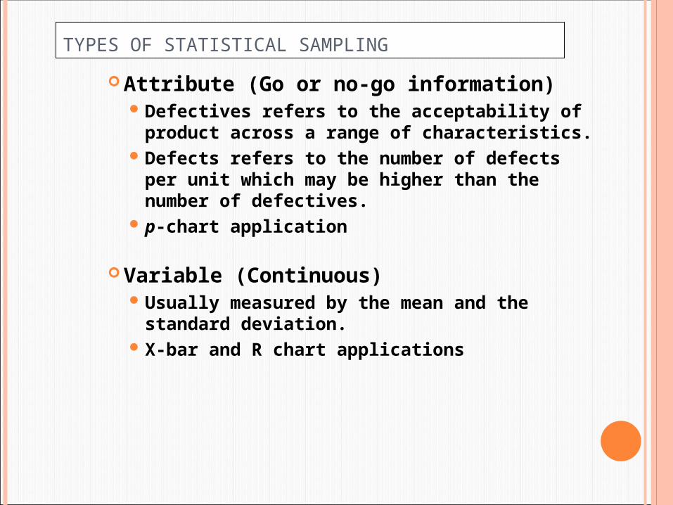
TYPES OF STATISTICAL SAMPLING
Attribute (Go or no-go information)Defectives refers to the acceptability of
product across a range of characteristics.Defects refers to the number of defects per
unit which may be higher than the number of defectives.
p-chart application
Variable (Continuous)Usually measured by the mean and the
standard deviation.X-bar and R chart applications

Statistical Process Control (SPC) Charts
UCL
LCL
Samples over time
1 2 3 4 5 6
UCL
LCL
Samples over time
1 2 3 4 5 6
UCL
LCL
Samples over time
1 2 3 4 5 6
Normal BehaviorNormal Behavior
Possible problem, investigatePossible problem, investigate
Possible problem, investigatePossible problem, investigate
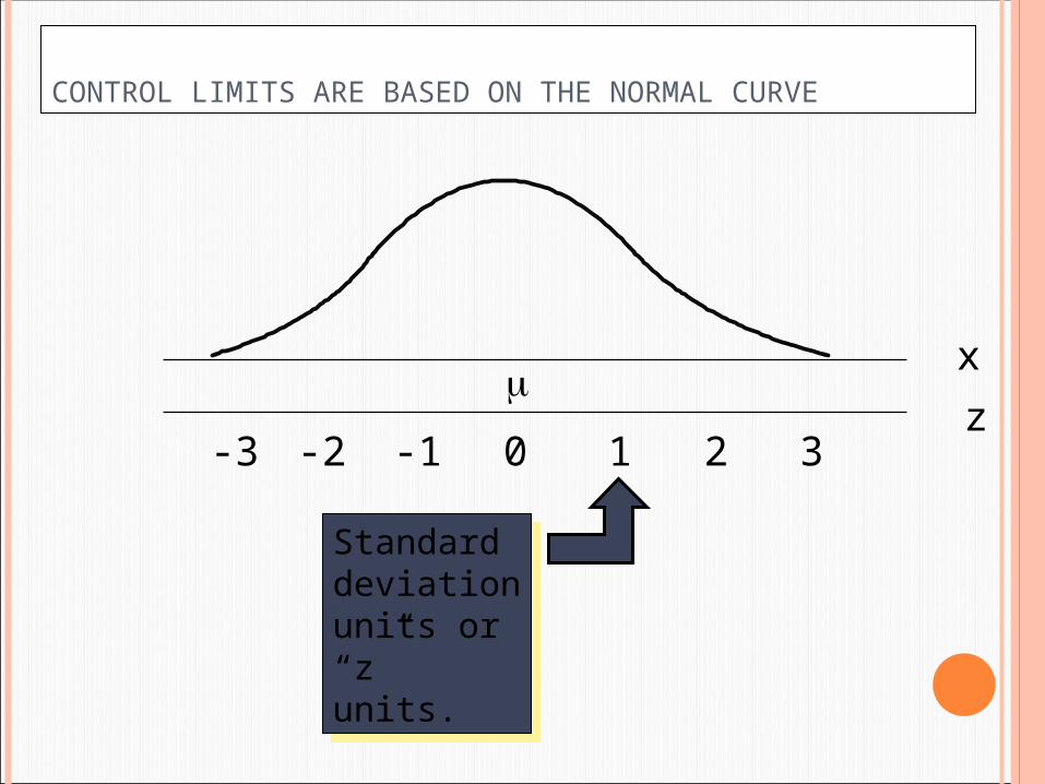
CONTROL LIMITS ARE BASED ON THE NORMAL CURVE
x
0 1 2 3-3 -2 -1z
Standard deviation units or “z” units.
Standard deviation units or “z” units.

CONTROL LIMITS
We establish the Upper Control Limits (UCL) and the Lower Control Limits (LCL) with plus or minus 3 standard deviations from some x-bar or mean value. Based on this we can expect 99.7% of our sample observations to fall within these limits.
xLCL UCL
99.7%

EXAMPLE OF CONSTRUCTING A P-CHART: REQUIRED DATA
1 100 42 100 23 100 54 100 35 100 66 100 47 100 38 100 79 100 1
10 100 211 100 312 100 213 100 214 100 815 100 3
Sample
No.
No. of
Samples
Number of defects found in each sample

STATISTICAL PROCESS CONTROL FORMULAS:ATTRIBUTE MEASUREMENTS (P-CHART)
p =Total Number of Defectives
Total Number of Observationsp =
Total Number of Defectives
Total Number of Observations
ns
)p-(1 p = p n
s)p-(1 p
= p
p
p
z - p = LCL
z + p = UCL
s
s
p
p
z - p = LCL
z + p = UCL
s
s
Given:
Compute control limits:
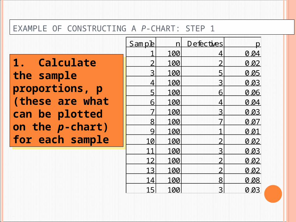
1. Calculate the sample proportions, p (these are what can be plotted on the p-chart) for each sample
1. Calculate the sample proportions, p (these are what can be plotted on the p-chart) for each sample
Sample n Defectives p1 100 4 0.042 100 2 0.023 100 5 0.054 100 3 0.035 100 6 0.066 100 4 0.047 100 3 0.038 100 7 0.079 100 1 0.01
10 100 2 0.0211 100 3 0.0312 100 2 0.0213 100 2 0.0214 100 8 0.0815 100 3 0.03
EXAMPLE OF CONSTRUCTING A P-CHART: STEP 1

2. Calculate the average of the sample proportions2. Calculate the average of the sample proportions
0.036=1500
55 = p 0.036=1500
55 = p
3. Calculate the standard deviation of the sample proportion 3. Calculate the standard deviation of the sample proportion
.0188= 100
.036)-.036(1=
)p-(1 p = p n
s .0188= 100
.036)-.036(1=
)p-(1 p = p n
s
EXAMPLE OF CONSTRUCTING A P-CHART: STEPS 2&3

4. Calculate the control limits4. Calculate the control limits
3(.0188) .036 3(.0188) .036
UCL = 0.0924LCL = -0.0204 (or 0)UCL = 0.0924LCL = -0.0204 (or 0)
p
p
z - p = LCL
z + p = UCL
s
s
p
p
z - p = LCL
z + p = UCL
s
s
EXAMPLE OF CONSTRUCTING A P-CHART: STEP 4
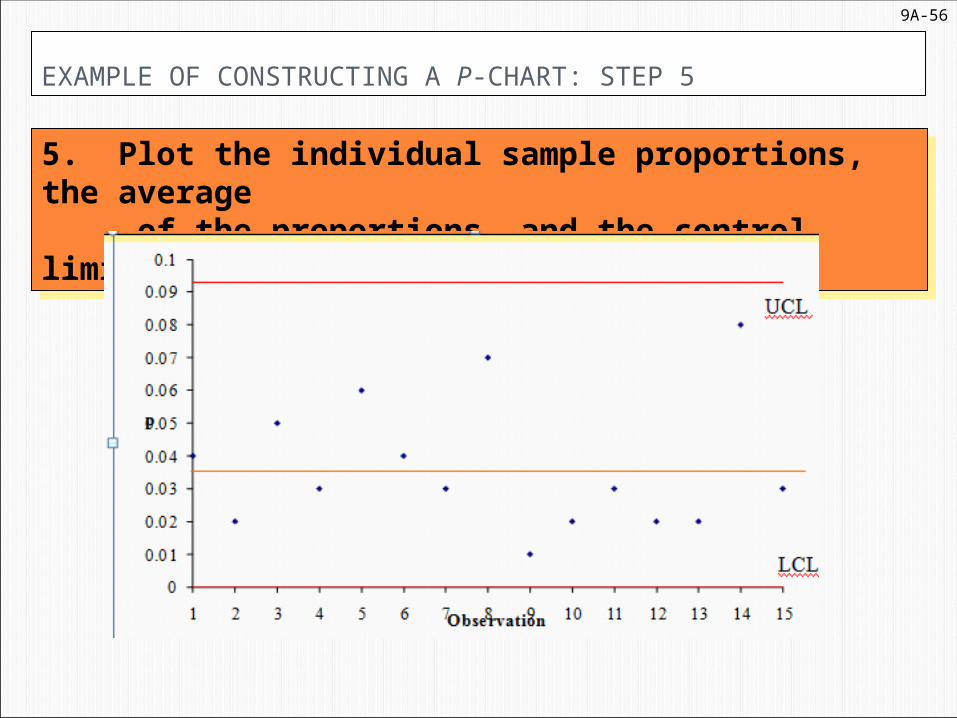
EXAMPLE OF CONSTRUCTING A P-CHART: STEP 5
5. Plot the individual sample proportions, the average of the proportions, and the control limits
5. Plot the individual sample proportions, the average of the proportions, and the control limits
9A-56

EXAMPLE OF X-BAR AND R CHARTS: REQUIRED DATA
Sample Obs 1 Obs 2 Obs 3 Obs 4 Obs 51 10.682 10.689 10.776 10.798 10.7142 10.787 10.86 10.601 10.746 10.7793 10.78 10.667 10.838 10.785 10.7234 10.591 10.727 10.812 10.775 10.735 10.693 10.708 10.79 10.758 10.6716 10.749 10.714 10.738 10.719 10.6067 10.791 10.713 10.689 10.877 10.6038 10.744 10.779 10.11 10.737 10.759 10.769 10.773 10.641 10.644 10.72510 10.718 10.671 10.708 10.85 10.71211 10.787 10.821 10.764 10.658 10.70812 10.622 10.802 10.818 10.872 10.72713 10.657 10.822 10.893 10.544 10.7514 10.806 10.749 10.859 10.801 10.70115 10.66 10.681 10.644 10.747 10.728

EXAMPLE OF X-BAR AND R CHARTS: STEP 1. CALCULATE SAMPLE MEANS, SAMPLE RANGES, MEAN OF MEANS, AND MEAN OF RANGES.
Sample Obs 1 Obs 2 Obs 3 Obs 4 Obs 5 Avg Range1 10.682 10.689 10.776 10.798 10.714 10.732 0.1162 10.787 10.86 10.601 10.746 10.779 10.755 0.2593 10.78 10.667 10.838 10.785 10.723 10.759 0.1714 10.591 10.727 10.812 10.775 10.73 10.727 0.2215 10.693 10.708 10.79 10.758 10.671 10.724 0.1196 10.749 10.714 10.738 10.719 10.606 10.705 0.1437 10.791 10.713 10.689 10.877 10.603 10.735 0.2748 10.744 10.779 10.11 10.737 10.75 10.624 0.6699 10.769 10.773 10.641 10.644 10.725 10.710 0.13210 10.718 10.671 10.708 10.85 10.712 10.732 0.17911 10.787 10.821 10.764 10.658 10.708 10.748 0.16312 10.622 10.802 10.818 10.872 10.727 10.768 0.25013 10.657 10.822 10.893 10.544 10.75 10.733 0.34914 10.806 10.749 10.859 10.801 10.701 10.783 0.15815 10.66 10.681 10.644 10.747 10.728 10.692 0.103
Averages 10.728 0.220400

EXAMPLE OF X-BAR AND R CHARTS: STEP 2. DETERMINE CONTROL LIMIT FORMULAS AND NECESSARY TABLED VALUES
x Chart Control Limits
UCL = x + A R
LCL = x - A R
2
2
x Chart Control Limits
UCL = x + A R
LCL = x - A R
2
2
R Chart Control Limits
UCL = D R
LCL = D R
4
3
R Chart Control Limits
UCL = D R
LCL = D R
4
3
From Exhibit TN 8.7From Exhibit TN 8.7
n A2 D3 D42 1.88 0 3.273 1.02 0 2.574 0.73 0 2.285 0.58 0 2.116 0.48 0 2.007 0.42 0.08 1.928 0.37 0.14 1.869 0.34 0.18 1.82
10 0.31 0.22 1.7811 0.29 0.26 1.74


EXAMPLE OF X-BAR AND R CHARTS: STEPS 3&4. CALCULATE X-BAR CHART AND PLOT VALUES
10.601
10.856
=).58(0.2204-10.728RA - x = LCL
=).58(0.2204-10.728RA + x = UCL
2
2
10.601
10.856
=).58(0.2204-10.728RA - x = LCL
=).58(0.2204-10.728RA + x = UCL
2
2
10.550
10.600
10.650
10.700
10.750
10.800
10.850
10.900
1 2 3 4 5 6 7 8 9 10 11 12 13 14 15
Sample
Mea
ns
UCL
LCL

EXAMPLE OF X-BAR AND R CHARTS: STEPS 5&6. CALCULATE R-CHART AND PLOT VALUES
0
0.46504
)2204.0)(0(R D= LCL
)2204.0)(11.2(R D= UCL
3
4
0
0.46504
)2204.0)(0(R D= LCL
)2204.0)(11.2(R D= UCL
3
4
UCL
LCL0.000
0.100
0.200
0.300
0.400
0.500
0.600
0.700
0.800
1 2 3 4 5 6 7 8 9 10 11 12 13 14 15
R
Sample


![MANUAL ON BENCHMARKING FOR QUALITY IMPROVEMENT OF …€¦ · 2012 [Manual on Benchmarking for Quality Improvement] FOREWORD Benchmarking is a performance improvement method that](https://static.fdocuments.in/doc/165x107/5f705b0f4ab5dd28605eb3c1/manual-on-benchmarking-for-quality-improvement-of-2012-manual-on-benchmarking-for.jpg)


