
Quality Assurance Project Plan Salish Sea Model Applications · Sound. The resulting Salish Sea...
94
Quality Assurance Project Plan Salish Sea Model Applications June 2018 Publication No. 18-03-111
Transcript of Quality Assurance Project Plan Salish Sea Model Applications · Sound. The resulting Salish Sea...

Quality Assurance Project Plan
Salish Sea Model Applications
June 2018
Publication No. 18-03-111
Publication Information
Each study conducted by the Washington State Department of Ecology (Ecology) must have an approved Quality Assurance Project Plan (QAPP). The plan describes the objectives of the study and the procedures to be followed to achieve those objectives. After completing the study,
Ecology will post the final report of the study to the Internet. This Quality Assurance Project Plan is available on Ecology’s website at https://fortress.wa.gov/ecy/publications/SummaryPages/1803111.html
Ecology’s Activity Tracker Code for this study is 06-509. This study is funded in part by the U.S. Environmental Protection Agency (EPA). Its contents do
not necessarily reflect the views and policies of the Environmental Protection Agency, nor does mention of trade names or commercial products constitute endorsement or recommendation for use.
Author and Contact Information Authors: Sheelagh McCarthy, Cristiana Figueroa-Kaminsky, Anise Ahmed, Teizeen Mohamedali, and Greg Pelletier
P.O. Box 47600 Environmental Assessment Program Washington State Department of Ecology
Olympia, WA 98504-7710 Ecology Communications Consultant: phone 360-407-7680.
Washington State Department of Ecology – https://ecology.wa.gov/
o Headquarters, Lacey 360-407-6000
o Northwest Regional Office, Bellevue 425-649-7000 o Southwest Regional Office, Lacey 360-407-6300 o Central Regional Office, Union Gap 509-575-2490
o Eastern Regional Office, Spokane 509-329-3400 Cover photo: Salish Sea Model domain.
Any use of product or firm names in this publication is for descriptive purposes only and
does not imply endorsement by the author or the Department of Ecology.
Accommodation Requests: To request ADA accommodation including materials in a format for the visually impaired, call Ecology at 360-407-6834. People with impaired hearing may call
Washington Relay Service at 711. People with speech disability may call TTY at 877-833-6341.
QAPP: Salish Sea Model Applications - Page 1 – June 2018
Template Version 1.0, 10/07/2016
Quality Assurance Project Plan
Salish Sea Model Applications
June 2018
Approved by:
Signature: Date:
Sheelagh McCarthy, Author / Salish Sea Modeling Team, EAP
Signature: Date:
Cristiana Figueroa-Kaminsky, Author / Project Manager, EAP
Signature: Date:
Dale Norton, Author’s Section Manager, EAP
Signature: Date:
Tom Gries, Acting Ecology Quality Assurance Officer
Signatures are not available on the Internet version.
EAP: Environmental Assessment Program

QAPP: Salish Sea Model Applications - Page 2 – June 2018
Template Version 1.0, 10/07/2016
1.0 Table of Contents Page
Acknowledgements ...................................................................................................... 6
2.0 Abstract ............................................................................................................ 7
3.0 Background....................................................................................................... 8 3.1 Introduction and problem statement ........................................................ 8 3.2 Study area and surroundings ..................................................................10
3.2.1 History of study area.....................................................................13
3.2.2 Summary of previous studies .....................................................14 3.2.3 Parameters of interest and potential sources ...............................18 3.2.4 Regulatory criteria or standards .................................................20
4.0 Project Description ...........................................................................................24
4.1 Project goals .........................................................................................24 4.2 Project objectives ..................................................................................24
4.2.1 Project objectives for SSM quality assurance guidance ..................24 4.2.1 Project objectives for model applications .......................................24
4.3 Information needed and sources.............................................................27 4.4 Tasks required ......................................................................................27 4.5 Systematic planning process used ..........................................................27
5.0 Organization and Schedule ...............................................................................28
5.1 Key individuals and their responsibilities ...............................................28 5.2 Special training and certifications ..........................................................28 5.3 Organization chart.................................................................................29 5.4 Proposed project schedule .....................................................................29
5.5 Budget and funding ...............................................................................29
6.0 Quality Objectives............................................................................................31 6.1 Data quality objectives ..........................................................................31 6.2 Measurement quality objectives .............................................................31
6.3 Acceptance criteria for quality of data ....................................................31 6.4 Model quality objectives .......................................................................33
7.0 Study Design....................................................................................................34 7.1 Study boundaries ..................................................................................34
7.2 Field data collection ..............................................................................35 7.3 Modeling and analysis design ................................................................35
7.3.1 Model setup and data needs...........................................................35 7.3.2 Boundary conditions .....................................................................38
7.3.3 Conducting model runs .................................................................42 7.4 Assumptions in relation to objectives and study area ..............................44 7.5 Possible challenges and contingencies ...................................................44
7.5.1 Logistical problems ......................................................................44
7.5.2 Practical constraints ......................................................................44 7.5.3 Schedule limitations .....................................................................45
8.0 Field Procedures...............................................................................................45 8.1 Invasive species evaluation....................................................................45

QAPP: Salish Sea Model Applications - Page 3 – June 2018
Template Version 1.0, 10/07/2016
8.2 Measurement and sampling procedures ..................................................45 8.3 Containers, preservation methods, holding times ....................................45 8.4 Equipment decontamination ..................................................................45
8.5 Sample ID ............................................................................................45 8.6 Chain-of-custody ..................................................................................45 8.7 Field log requirements ...........................................................................45 8.8 Other activities......................................................................................45
9.0 Laboratory Procedures......................................................................................46 9.1 Lab procedures table .............................................................................46 9.2 Sample preparation method(s) ...............................................................46 9.3 Special method requirements .................................................................46
9.4 Laboratories accredited for methods ......................................................46
10.0 Quality Control Procedures...............................................................................46 10.1 Table of field and laboratory quality control...........................................46 10.2 Corrective action processes ...................................................................46
11.0 Data Management Procedures...........................................................................47 11.1 Data recording and reporting requirements .............................................47 11.2 Laboratory data package requirements ...................................................47 11.3 Electronic transfer requirements ............................................................47
11.4 EIM/STORET data upload procedures ...................................................48 11.5 Model information management ............................................................48
11.5.1 Cluster computer data management .............................................48 11.5.2 Project input and output files .......................................................48
11.5.3 Modeling project folders .............................................................49
12.0 Audits and Reports ...........................................................................................51 12.1 Field, laboratory, and other audits ..........................................................51 12.2 Responsible personnel ...........................................................................51
12.3 Frequency and distribution of reports .....................................................51 12.4 Responsibility for reports ......................................................................51
13.0 Data Verification..............................................................................................52 13.1 Field data verification, requirements, and responsibilities .......................52
13.2 Laboratory data verification...................................................................52 13.3 Validation requirements, if necessary.....................................................52 13.4 Model quality assessment ......................................................................52
13.4.1 Calibration and evaluation...........................................................52
13.4.2 Sensitivity and uncertainty analyses ............................................55
14.0 Data Quality (Usability) Assessment .................................................................57 14.1 Process for determining project objectives were met...............................57 14.2 Treatment of non-detects .......................................................................57
14.3 Data analysis and presentation methods .................................................58 14.4 Sampling design evaluation ...................................................................58 14.5 Documentation of assessment ................................................................58
15.0 References .......................................................................................................59
16.0 Appendices ......................................................................................................67 Appendix A. Existing data sources and information ..........................................68

QAPP: Salish Sea Model Applications - Page 4 – June 2018
Template Version 1.0, 10/07/2016
Appendix B. Model versions.............................................................................74 Appendix C. Parameters and rates.....................................................................76 Appendix D. Model equations ..........................................................................78
Appendix E. Method of evaluation of predicted violations of the DO criteria......83 Appendix F. Glossaries, acronyms, and abbreviations........................................84

QAPP: Salish Sea Model Applications - Page 5 – June 2018
Template Version 1.0, 10/07/2016
List of Figures and Tables Page
Figure 1. Map of Salish Sea study area. ........................................................................10
Figure 2. Timeline of Salish Sea Model related publications..........................................16
Figure 3. 303(d) listings for dissolved oxygen in Puget Sound. ......................................19
Figure 4. Map of dissolved oxygen Water Quality Standards for Puget Sound. ..............21
Figure 5. Map of pH Water Quality Standards for Puget Sound. ....................................22
Figure 6. Salish Sea Model expanded grid model domain. .............................................34
Figure 7. Biogeochemical processes diagram for the Salish Sea Model (Pelletier et al., 2017b) ..........................................................................................................37
Figure 8. Residence time index for the Central Puget Sound basin during summer months, (Albertson et al., 2016). ....................................................................43
Figure 9. Example of an ArcGIS Online web map that shows model output for existing conditions for annual average DO in bottom layer during 2006. ......................47
Figure 10. Folder and file management structure for the modeling server.......................50
Figure 11. Comparison of model results with observational data for dissolved oxygen
(DO) in Padilla Bay. .....................................................................................55
Table 1. Summary of studies and reports related to the Salish Sea Model. ......................14
Table 2. Regulatory marine water designated uses and criteria for dissolved oxygen in
Washington State (WAC 173-201A-210). ......................................................20
Table 3. Regulatory marine water designated uses and criteria for pH in Washington
State (WAC 173-201A-210)..........................................................................21
Table 4. Organization of project staff and responsibilities. ............................................28
Table 5. Proposed project schedule for modeling work and written documents for the
Puget Sound Nutrient Source Reduction Project (PSNSRP)............................29
Table 6. Proposed budget and funding for modeling work for the Puget Sound
Nutrient Reduction Project (PSNSRP). ..........................................................30
Table 7. Salish Sea model versions. ..............................................................................35
Table 8. Summary of data needs for model inputs for the hydrodynamic and water
quality model. ...............................................................................................36

QAPP: Salish Sea Model Applications - Page 6 – June 2018
Template Version 1.0, 10/07/2016
Acknowledgements
This project received funding from grants to the Washington State Department of Ecology (Ecology) from the United States Environmental Protection Agency (EPA), National Estuarine Program, under EPA grant agreements PC-00J20101 and PC00J89901, Catalog of Domestic
Assistance Number 66.123, Puget Sound Action Agenda: Technical Investigations and Implementation Assistance Program. The content of this document does not necessarily reflect the views and policies of EPA, nor does mention of trade names or commercial products constitute an endorsement or a recommendation for their use.
The authors of this QAPP thank the following people for their contributions in reviewing this document:
Dustin Bilhimer (Ecology)
Ben Cope (US EPA)
Tom Gries (Ecology)
Paul Pickett (Ecology)
We also thank Joan LeTourneau and Ruth Froese for their help with publication.

QAPP: Salish Sea Model Applications - Page 7 – June 2018
Template Version 1.0, 10/07/2016
2.0 Abstract
Puget Sound has areas with low levels of dissolved oxygen (DO) that do not meet Washington State’s Water Quality Standards. Recent modeling work and studies indicate that low DO concentrations in Puget Sound are influenced by naturally occurring low DO waters from the
Pacific Ocean and also, increasingly, by human nutrient contributions. Pacific Northwest National Laboratory, in collaboration with the Washington State Department of Ecology (Ecology), developed a three-dimensional circulation and water quality model to
simulate the processes affecting DO and water quality throughout the Salish Sea, including Puget Sound. The resulting Salish Sea Model (SSM) is a tool used to evaluate human impacts on water quality conditions in the Puget Sound region using the best available information.
This Quality Assurance Project Plan (QAPP) serves as a guidance document summarizing information from previous SSM-related QAPPs and model development publications. This QAPP also describes the modeling and quality assurance procedures that are used to optimize and assess model performance.
Ecology will use the SSM to estimate current conditions, as well as water quality outcomes, under different modeling scenarios. This work will be used as part of Ecology’s Puget Sound Nutrient Source Reduction Project (PSNSRP) to evaluate options for nutrient reduction from
point and nonpoint sources in Washington. This project will develop distinct modeling and optimization scenarios to assess nutrient reduction options in order to improve DO levels and water quality in Puget Sound.
Although emphasis is placed on model applications for the PSNSRP, this QAPP may also be applied to any related SSM runs conducted to predict water quality conditions in the Salish Sea. These applications could include ocean acidification investigations, climate change predictions, scenarios specific to restoration efforts, or model runs restricted to a sub-region of the model
domain.

QAPP: Salish Sea Model Applications - Page 8 – June 2018
Template Version 1.0, 10/07/2016
3.0 Background
3.1 Introduction and problem statement
Low dissolved oxygen (DO) levels have been observed in many areas throughout Puget Sound over recent years. Previous research and studies have shown that increased nutrient inputs, particularly nitrogen and carbon, from anthropogenic sources have influenced low DO levels in
Puget Sound (Banas et al., 2015; Glibert et al., 2005; Howarth, 2008; Newton and Van Voorhis, 2002; Pelletier, 2017a). Pacific Northwest National Laboratory (PNNL), in collaboration with Washington State
Department of Ecology (Ecology), developed the Salish Sea Model (SSM) as a predictive ocean-modeling tool for coastal estuarine research, restoration planning, water-quality management, and climate change response assessment. The SSM was originally developed to evaluate the influence of human activity from watershed runoff and wastewater discharges on low DO levels
and water quality in Puget Sound. The model was expanded to include the entire Salish Sea, including Puget Sound, Strait of Juan de Fuca, and Strait of Georgia (Figure 1). Since original development of the SSM (previously called the Puget Sound Dissolved Oxygen
Model) in 2009, the model has been updated and improved to better simulate water quality conditions of the Salish Sea. Over the course of these different stages of development and improvements to the SSM, there have been a series of model-related publications and Quality Assurance Project Plans (QAPPs). These documents describe the different scales of the model
framework, hydrodynamics, water quality modeling, nutrient loading, data needs, and intended model applications.
Ecology will apply the SSM as part of their work with the Puget Sound Nutrient Reduction Project (PSNSRP). PSNSRP is addressing human sources of nutrients from point and nonpoint sources and seeks to develop and implement a Puget Sound nutrient source reduction plan. The
plan will guide regional investments in point and nonpoint source nutrient controls so that Puget Sound will meet DO water quality criteria and aquatic life designated uses by 2040. The goals of these reductions are to:
Meet water quality standards for Puget Sound.
Provide a technical basis for exercising National Pollutant Discharge Elimination System (NPDES) authority for nutrient water quality-based effluent limits.
Address nonpoint nutrient sources under the Washington State Water Pollution Control Act (RCW 90.48).
Protect and restore Puget Sound into the future, given the expected stresses associated with climate change and additional nutrient loading due to future population growth.
Ecology may also apply the SSM to simulate carbonate system chemistry and ocean acidification scenarios in the Salish Sea. To date, SSM runs have been conducted and documented for 2008 (Pelletier et al., 2017b). However, more data and observations are now available for recent years, and the SSM can be used to predict the spatial and temporal variability during those additional
QAPP: Salish Sea Model Applications - Page 9 – June 2018
Template Version 1.0, 10/07/2016
years. The SSM will continue to be used to evaluate ocean acidification and other related water quality applications for the Salish Sea years into the future.
This QAPP summarizes and references key points and material from previous model development publications as it applies to the current version of the SSM. It describes major changes to the model through its different development stages and includes information for the latest version of the model framework and setup. This modeling work will use the SSM for
model applications to simulate water quality conditions in the Puget Sound region. Particularly, the SSM will be used to evaluate nutrient source reduction scenarios. It may also be used for other water quality modeling work related to the Salish Sea, including ocean acidification and future conditions.
The development of the SSM has produced multiple versions of a calibrated model simulating water quality conditions in the Salish Sea. Section 7.3.2 provides more details for each model version (e.g. PSM2, SSM2). The term ‘SSM’ is applied collectively to describe these models
throughout this document. This QAPP includes information and updates from earlier versions of the SSM; however, the QA procedures can be applied to both the most recently calibrated model version (SSM2) and the earlier calibrated versions (e.g. PSM2). Using earlier versions of the SSM may be necessary for logistical and practical reasons.
QAPP: Salish Sea Model Applications - Page 10 – June 2018
Template Version 1.0, 10/07/2016
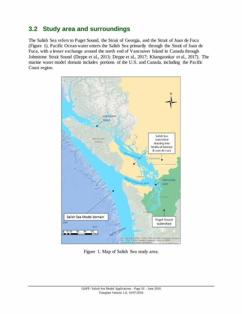
3.2 Study area and surroundings
The Salish Sea refers to Puget Sound, the Strait of Georgia, and the Strait of Juan de Fuca (Figure 1). Pacific Ocean water enters the Salish Sea primarily through the Strait of Juan de Fuca, with a lesser exchange around the north end of Vancouver Island in Canada through
Johnstone Strait Sound (Deppe et al., 2013; Deppe et al., 2017; Khangaonkar et al., 2017). The marine water model domain includes portions of the U.S. and Canada, including the Pacific Coast region.
Figure 1. Map of Salish Sea study area.

QAPP: Salish Sea Model Applications - Page 11 – June 2018
Template Version 1.0, 10/07/2016
Estuarine waters exhibit highly complex circulation patterns. Circulation in the Salish Sea is influenced by the intricate morphological configuration of its individual basins and bathymetry (Cannon, 1983). Shallow sills occur at the entrances to various basins, including Hood Canal,
Admiralty Inlet, and the Tacoma Narrows (Deppe et al., 2017; Ebbesmeyer et al., 1984; Geyer and Cannon, 1982). The Pacific Ocean influences circulation and conditions in Puget Sound. Upwelling conditions from the Pacific Ocean vary in strength and duration, with short-term intrusions over the sill at Admiralty Inlet that bring in water low in DO, aragonite saturation
state, and pH into Puget Sound (Deppe et al., 2013; Deppe et al., 2017; Khangaonkar et al., 2017). Stratification affects vertical mixing throughout the Salish Sea as well, and it shows a strong
two-layer circulation pattern (Cannon et al., 2001; Geyer and Cannon, 1982; Khangaonkar et al., 2011; Morrison et al., 2012). Water is continuously mixed and flushed based on freshwater inflows from rivers and also outflows to the Pacific Ocean. Longer flushing times (the turnover time of freshwater in an estuary) occur in the inlets and contribute to low DO levels in these
areas (Ahmed et al., 2017; Sutherland et al., 2011). Puget Sound is the marine water south of Admiralty Inlet (Figure 1), and the Sound receives varying freshwater inflows dependent on seasonal conditions. The largest direct source of
freshwater to Puget Sound is the Skagit River, which flows into the Whidbey Basin and receives water from the Stillaguamish and Snohomish Rivers (Khangaonkar et al., 2016, 2017). The Fraser River, flowing from Canada and into the Salish Sea north of Admiralty Inlet, also indirectly influences Puget Sound (Banas et al., 2015; Khangaonkar and Xu, 2017; Khangaonkar
et al., 2018b). The major watersheds that drain into Central Puget Sound include the Cedar, Green, and Puyallup Rivers along with freshwater from portions of the Puget Lowland to the east and west. Hood Canal receives water flowing from the eastern Olympic Mountains and the western Kitsap Peninsula. The Nisqually and Deschutes Rivers are the largest rivers that drain
into South Puget Sound. Freshwater from the Puget Lowlands also flow into South Puget Sound. Recent studies have shown that nitrogen is a limiting nutrient in Puget Sound waters (Howarth and Marino, 2006; Newton and Van Voorhis, 2002). Nitrogen naturally occurs in rivers and
streams entering marine waters through sources and pathways of atmospheric deposition, salmon and biological activity, and forested land processes (Brandenberger et al., 2011; Glibert et al., 2005). Watershed inflows that enter Puget Sound deliver loads (where loads are quantified as concentration multiplied by flow) of nitrogen and other nutrients.
Human activities have increased nitrogen loads above naturally occurring levels in Puget Sound (Mohamedali et al., 2011). Both point and nonpoint human sources produce nitrogen loadings. Marine point sources include wastewater treatment plants (WWTPs), industrial facilities, and
other discharges. Nonpoint sources include releases from residential, commercial, and industrial land uses; agriculture; septic systems; and other activities. Watershed nitrogen loading is seasonally dependent on river flow, sources of nitrogen, and fate and transport processes that use up nitrogen (e.g. plant uptake, denitrification).
Rivers and other freshwaters deliver nitrogen, predominantly as dissolved inorganic nitrogen (DIN; the sum of nitrate and ammonia), as well as organic carbon and other nutrients to the estuarine environment. In 2006, U.S. watersheds delivered an estimated annual average of

QAPP: Salish Sea Model Applications - Page 12 – June 2018
Template Version 1.0, 10/07/2016
27,500 kg/d of DIN to Puget Sound and an additional 7,300 kg/d to the Straits from the combined effect of natural and human sources (Mohamedali et al., 2011). Canadian watersheds delivered an estimated 44,400 kg/d of DIN, dominated by the Fraser River with 33,500 kg/d.
These include the combined effect of natural and human sources within the watersheds. WWTPs also discharge nutrient-laden effluent, including the nutrients carbon and nitrogen. Inventoried point sources discharging directly into marine waters deliver much less flow than the
watersheds. U.S. marine point sources produce 20 m3/s, and Canadian marine point sources produce about 16 m3/s (Mohamedali et al., 2011). However, nitrogen is more concentrated in WWTP effluent and can be 10 to 30 mg/L of total nitrogen, nearly all of which is DIN. This results in annual average nutrient loads from treated wastewater of approximately 32,600 kg/d
from U.S. WWTPs and 29,100 kg/d of DIN from Canadian WWTPs in 2006. Nearly all of the wastewater is from municipal wastewater; a small fraction is from industrial wastewater. The largest wastewater inputs are from the largest metropolitan areas.
Organic carbon is also a key nutrient found in the water column and bottom sediments that fuels biogeochemical reactions that can lead to hypoxia and ocean acidification (Howarth, 2008; Feely et al., 2010). Acidification is increased by regional anthropogenic nutrient sources because the increase in primary production and organic carbon loading leads to increased respiration and
release of carbon dioxide because of increased decay of organic matter. Increased organic carbon caused by regional anthropogenic nutrient sources can significantly contribute to acidification in the Salish Sea (Pelletier et al., 2017b).
Non-algal organic carbon represents the pool of organic carbon that is subject to release of carbon dioxide by heterotrophic metabolism, including detrital particulate organic carbon and dissolved organic carbon (Chan et al., 2016; Long et al., 2014). Regional anthropogenic sources account for up to around 35% of the May-September average non-algal organic carbon in the
surface 20 meters, with fractions of 20% to 25% fairly widespread through most of the main basin of Puget Sound, inner Budd Inlet, and Port Susan/Possession Sound (Pelletier et al., 2017b). Around 10% to 15% of the non-algal organic carbon in Saratoga Passage and Admiralty Inlet is due to regional anthropogenic sources. These anthropogenic sources account for about
5% to 10% of the non-algal organic carbon in Hood Canal.
A portion of the non-algal organic carbon that is attributed to regional anthropogenic sources is
derived from an increase in detritus resulting from increased primary production (autochthonous), and part is from direct loading of watershed sources from rivers and WWTPs (allochthonous) (Pelletier et al., 2017b). Additional studies are needed to quantify the amount from each source and to distinguish between the various allochthonous sources.
Population is projected to continue to increase in the Puget Sound watershed. This will result in increased human activity and development, as well as a concomitant increase in wastewater effluent flows (Khangaonkar et al., 2016; Mohamedali et al., 2011; Roberts et al., 2014a).
Changes in climate are also expected to affect both water quantity and quality in the region (Khangaonkar et al., 2018a; Mote et al., 2014; Snover et al., 2013). Factors affecting these changes include (1) natural climate variability, which influences regional climate and hydrology on annual and decadal scales and (2) long-term increases in air temperature due to rising
greenhouse gas emissions.

QAPP: Salish Sea Model Applications - Page 13 – June 2018
Template Version 1.0, 10/07/2016
In 2015, the University of Washington Climate Impacts Group published State of Knowledge: Climate Change in Puget Sound (Mauger et al., 2015). This report summarized current research
on the impacts of climate change in the Puget Sound region for issues ranging from snowpack to human health. The report identified numerous likely changes in freshwater and marine water quality. These changes include:
Decreased summer freshwater flows.
Increased sediment loads in winter and spring.
Increased nutrient inputs from human activities.
Warmer freshwater and marine water temperatures.
Decreased DO levels.
Changes in estuarine circulation.
Increased harmful algal blooms.
Increased acidification (lower marine pH levels).
Rising sea levels and increased coastal erosion. Additionally, a climate change scenarios report using the SSM showed the influence of climate
change on the Salish Sea (Khangaonkar et al., 2018a). This study found that under future climate change scenarios, the Salish Sea will see an overall increase in temperature, depletion of DO levels, a shift of algal species towards those with preference for higher temperatures, and continued ocean acidification.
3.2.1 History of study area
Sackmann (2009) provides an in-depth history of the study area. In summary, low DO has been measured in several locations within the Salish Sea, and these low DO levels are influenced by
nutrients, particularly nitrogen and organic carbon. Although eutrophication exists as a natural process, the increase in anthropogenic nutrient pollution can cause cultural eutrophication, which is the process of enhanced eutrophication resulting from human activity. Both natural and cultural eutrophication occur when a body of water becomes enriched with nutrients, such as
nitrogen and carbon, which stimulates excessive algal growth. Decomposition and respiration of excessive algae by bacteria results in oxygen consumption. This leads to DO depletion in areas that are not well aerated, such as shallow embayments and near-bottom waters.
Various research projects and studies have focused on investigating whether human contributions are responsible for declining DO levels over time in Puget Sound. Recent studies have shown an increasing recognition that over-enrichment of nutrients from human sources contributes to DO problems (Banas et al., 2015; Glibert et al., 2005; Howarth, 2008;
Mohamedali et al., 2011; Newton and Van Voorhis, 2002; Roberts et al., 2014; Pelletier, 2017a,b; PSEMP Marine Waters Workgroup, 2017). These excess nutrients contribute to degradation of habitat quality, loss of biotic diversity, and increased harmful algal blooms (Glibert et al., 2005; Howarth, 2008).
Excess nitrogen has been the predominant nutrient studied for the effects of eutrophication on Puget Sound (Newton and Van Voorhis, 2002). However, organic carbon in the water column
QAPP: Salish Sea Model Applications - Page 14 – June 2018
Template Version 1.0, 10/07/2016
and bottom sediments is also influential as it fuels biogeochemical reactions that can lead to hypoxia and ocean acidification (Feely et al., 2010; Howarth, 2008; Pelletier et al., 2017b).
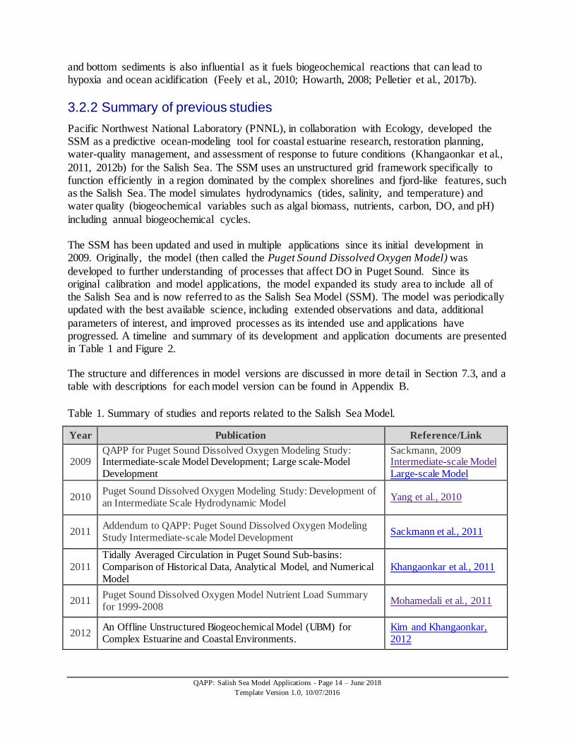
3.2.2 Summary of previous studies
Pacific Northwest National Laboratory (PNNL), in collaboration with Ecology, developed the SSM as a predictive ocean-modeling tool for coastal estuarine research, restoration planning, water-quality management, and assessment of response to future conditions (Khangaonkar et al.,
2011, 2012b) for the Salish Sea. The SSM uses an unstructured grid framework specifically to function efficiently in a region dominated by the complex shorelines and fjord-like features, such as the Salish Sea. The model simulates hydrodynamics (tides, salinity, and temperature) and water quality (biogeochemical variables such as algal biomass, nutrients, carbon, DO, and pH)
including annual biogeochemical cycles. The SSM has been updated and used in multiple applications since its initial development in 2009. Originally, the model (then called the Puget Sound Dissolved Oxygen Model) was
developed to further understanding of processes that affect DO in Puget Sound. Since its original calibration and model applications, the model expanded its study area to include all of the Salish Sea and is now referred to as the Salish Sea Model (SSM). The model was periodically updated with the best available science, including extended observations and data, additional
parameters of interest, and improved processes as its intended use and applications have progressed. A timeline and summary of its development and application documents are presented in Table 1 and Figure 2.
The structure and differences in model versions are discussed in more detail in Section 7.3, and a table with descriptions for each model version can be found in Appendix B.
Table 1. Summary of studies and reports related to the Salish Sea Model.
Year Publication Reference/Link
2009 QAPP for Puget Sound Dissolved Oxygen Modeling Study: Intermediate-scale Model Development; Large scale-Model
Development
Sackmann, 2009 Intermediate-scale Model
Large-scale Model
2010 Puget Sound Dissolved Oxygen Modeling Study: Development of
an Intermediate Scale Hydrodynamic Model Yang et al., 2010
2011 Addendum to QAPP: Puget Sound Dissolved Oxygen Modeling
Study Intermediate-scale Model Development Sackmann et al., 2011
2011
Tidally Averaged Circulation in Puget Sound Sub-basins:
Comparison of Historical Data, Analytical Model, and Numerical
Model
Khangaonkar et al., 2011
2011 Puget Sound Dissolved Oxygen Model Nutrient Load Summary
for 1999-2008 Mohamedali et al., 2011
2012 An Offline Unstructured Biogeochemical Model (UBM) for
Complex Estuarine and Coastal Environments.
Kim and Khangaonkar,
2012

QAPP: Salish Sea Model Applications - Page 15 – June 2018
Template Version 1.0, 10/07/2016
Year Publication Reference/Link
2012 Puget Sound Dissolved Oxygen Modeling Study: Development of an Intermediate Scale Water Quality Model
Khangaonkar et al., 2012a
2012
Simulation of annual biogeochemical cycles of nutrient balance,
phytoplankton bloom(s), and dissolved oxygen in Puget Sound
using an unstructured grid model
Khangaonkar et al., 2012b
2014 South Puget Sound Dissolved Oxygen Study: Water Quality
Model Calibrations and Scenarios Ahmed et al., 2014
2014
Sound and the Straits Dissolved Oxygen Assessment: Impacts of
Current and Future Human Nitrogen Sources and Climate Change through 2070
Roberts et al., 2014a
2014 Approach for Simulating Acidification and the Carbon Cycle in
the Salish Sea to Distinguish Regional Source Impacts Long et al., 2014
2015 QAPP: Salish Sea Dissolved Oxygen Modeling Approach:
Sediment-Water Interactions Roberts et al., 2015a
2015 QAPP: Salish Sea Acidification Model Development Roberts et al. 2015b
2017 Assessment of Circulation and Inter-basin Transport in the Salish
Sea including Johnstone Strait and Discovery Islands Pathways Khangaonkar et al., 2017
2017 Salish Sea Model: Sediment Diagenesis Module Pelletier et al., 2017a
2017 Salish Sea Model, Ocean Acidification Module and the Response
to Regional Anthropogenic Nutrient Sources Pelletier et al., 2017b
2018 Sensitivity of the Regional Ocean Acidification and the Carbonate
System in Puget Sound to Ocean and Freshwater Inputs Bianucci et al., 2018
2018 Simulation of Response to Climate Change and Sea Level Rise
Scenarios Khangaonkar et al, 2018a
2018 Analysis of Hypoxia and Sensitivity to Nutrient Pollution in Salish
Sea Khangaonkar et al., 2018b
2018 QAPP: Salish Sea Model Applications This work.
QAPP: Quality Assurance Project Plan

QAPP: Salish Sea Model Applications - Page 16 – June 2018
Template Version 1.0, 10/07/2016
Figure 2. Timeline of Salish Sea Model related publications.
Light arrows indicate QAPP and model development and QAPP documents.
Dark arrows indicate technical reports and journal articles.

QAPP: Salish Sea Model Applications - Page 17 – June 2018
Template Version 1.0, 10/07/2016
In 2009, two QAPPs were published for development of the large-scale Puget Sound box model and intermediate-scale Puget Sound Dissolved Oxygen Model (Sackmann, 2009). These models were developed in tandem to determine nitrogen loadings and anthropogenic impacts on DO
levels. The large-scale box model consisted of a coarse spatial resolution, but was computationally efficient and allowed for rapid evaluation of multiple nutrient loading scenarios. The large-scale model was used as a screening-level tool to support the intermediate-scale modeling effort. The intermediate-scale hydrodynamic and water quality model was used to
develop a better understanding of the nutrient assimilation capacity of Puget Sound. Both models were calibrated with observations from Puget Sound (Khangaonkar et al., 2011a,b and 2012). A nutrient load summary for 1998-2008 was published to be used during the intermediate-scale
model scenario runs (Mohamedali et al., 2011). This report presents the magnitudes and sources of nitrogen loading into Puget Sound, Straits of Georgia, and Juan de Fuca from all point and nonpoint sources (e.g. rivers and WWTPs) within the model domain.
In 2014, Ecology completed an analysis of the relative influences of human nutrient sources and Pacific Ocean influences on DO concentrations in the Salish Sea. This analysis involved applying the model to a series of scenarios to isolate the influence on DO from different sources, both now and into the future (Roberts et al., 2014a). This was a first assessment of how the
Salish Sea DO concentrations respond to population increases, ocean conditions, and climate change. However, this work did not include sediment water interactions, but it did help to recognize the importance of this key process on DO levels in bottom waters.
Ahmed et al. (2014), using a different model limited to South and Central Puget Sound marine waters, concluded that human sources decrease DO by up to about 0.38 mg/L below natural conditions, and recommended continued coordination with the larger SSM effort, as well as adding the capability to dynamically simulate sediment-water exchanges. This work was part of
the South Puget Sound Dissolved Oxygen Study (Ahmed et al., 2014). There is a separate report for model development and calibration for the water circulation of South and Central Puget Sound (Roberts et al., 2014b).
Based on the modeling analysis and results published in 2014 (Ahmed et al., 2014; Roberts et al., 2014a), a Sediment Diagenesis Module was added to the SSM and a report discussing the results of this analysis was published in 2017 (Pelletier et al., 2017a). Sediment diagenesis occurs when water column material fluxes to the sediment and fuels biogeochemical processes that release
some of the nutrients back to the water column and consume oxygen in the process. Because sediment-water interactions strongly influence oxygen levels, this update to the SSM improved the ability to distinguish the effects of individual nutrient sources on sediment fluxes and DO levels in the Salish Sea. The study involved re-calibrating the model with observational data
resulting in improvements for predicting lower ranges of DO, particularly in the bottom layer. An Ocean Acidification Module was also developed for the SSM (Bianucci et al., 2018; Pelletier et al., 2017b). This Ocean Acidification Module is used to model processes influencing ocean
acidification by evaluating aragonite saturation state (Ωarag) and related carbonate system variables. It is used in assessing the ability for calcifying organisms to build shells. This study examined and quantified how regional freshwater and land-derived sources of nutrients generally impact acidification in the Salish Sea. The SSM was expanded by adding total dissolved

QAPP: Salish Sea Model Applications - Page 18 – June 2018
Template Version 1.0, 10/07/2016
inorganic carbon (DIC) and alkalinity as state variables, including source and sink terms related to air-sea exchange, respiration, photosynthesis, nutrient gains and losses, sediment fluxes, and boundary conditions.
A recent report evaluated the impacts of different climate change scenarios to the Salish Sea (Khangaonkar et al., 2018a). This study used the expanded grid version of the model, where the model domain extends to the continental shelf, and also the Ocean Acidification and Sediment
Diagenesis Modules. For model inputs, results were extracted from (1) a global circulation model from the National Center for Climate Research and (2) the Community Earth System Model (CESM) from the Intergovernmental Panel on Climate Change’s 5th assessment report. This work used the historical emissions and a future high-emission scenario titled RCP8.5. In
order to compare future scenarios with baseline conditions, simulations from 1995-2004 were averaged to represent the year (Y) 2000 scenario to represent “present conditions.” These were used as inputs to SSM. The future scenario was defined by conditions averaged over 10 years of simulation from 2091 to 2100 (Y2095 RCP8.5 scenario).
The model results from the climate change scenarios showed that responses to the Salish Sea under the RCP8.5 emissions scenario included overall warming, depletion of DO levels, shift of algal species towards those with preference for higher temperatures, and continued ocean
acidification (Khangaonkar et al., 2018a). Throughout the Salish Sea, there was an average increase in temperature of 1.8°C, decrease in DO of 0.7 mg/L, and reduction in pH of 0.12 when comparing the predicted Y2095 with baseline Y2000 conditions. Algal biomass is predicted to increase by 23%, and the region of annually recurring hypoxia that occupies <1% of the Salish
Sea in Y2000 conditions is predicted to cover nearly 16% in the future. The results from the climate change scenarios report also showed that the Salish Sea response in the future is less severe in magnitude when compared to the global change as reflected in the
outer ocean near the edge of the continental shelf (Khangaonkar et al., 2018a). This is attributed to benefits from the existence of strong estuarine circulation and healthy primary production in the Salish Sea.
The SSM was used to run multiple sensitivity tests to evaluate the response of the Salish Sea to rivers and nutrient loadings (Khangaonkar, 2018b). This study used the expanded grid version of the model, where the model domain encompasses Vancouver Island and extends to the continental shelf. It also included the updates of the Sediment Diagenesis and Ocean
Acidification Modules. Results from this study showed the large impacts of the Fraser River on the magnitude of estuarine exchange with the Pacific Ocean and nearshore habitat, with a lesser influence on exchange to Puget Sound through Admiralty Inlet. The SSM simulated an area of large hypoxia in Hood Canal and demonstrated the responsiveness of the Salish Sea to changes
in nutrient loads to the euphotic zone.
3.2.3 Parameters of interest and potential sources
The primary parameter of concern for this work is DO; however, other important water quality
(WQ) parameters simulated in SSM include temperature, phytoplankton biomass, pH, nitrogen, and aragonite.

QAPP: Salish Sea Model Applications - Page 19 – June 2018
Template Version 1.0, 10/07/2016
DO is strongly influenced by the biogeochemical cycling of nutrients. Nutrients from local natural and human sources, the Pacific Ocean, and atmospheric sources stimulate phytoplankton growth and autotrophic and heterotrophic respiration. Organic matter containing carbon and
nitrogen is produced as phytoplankton die and sink to the bottom. Oxygen is consumed during oxidation of the decomposing organic matter, and some of the organic nitrogen is re-mineralized and released back into the water. Therefore, nitrogen and carbon contributions , specifically dissolved inorganic nitrogen (DIN) and total organic carbon (TOC), are key parameters for
understanding DO impairments.
Figure 3 shows areas of Puget Sound listed on Washington State’s 303(d) list of impaired waters
for DO.
Figure 3. 303(d) listings for dissolved oxygen in Puget Sound.
Red indicates Category 5 impaired waters; gray represents Category 2 areas of concern) (2014).
Areas shown on Figure 3 include both Category 5 (impaired) waters and Category 2 (areas of concern). For all marine waters in Puget Sound and Washington State waters in the Straits of Juan de Fuca and Georgia, there is a total of 102 Category 5 listings and 321 Category 2 listings for DO based on the 2014 Water Quality Assessment.

QAPP: Salish Sea Model Applications - Page 20 – June 2018
Template Version 1.0, 10/07/2016
Aragonite saturation state (Ωar) is also included in this analysis, as it is an indicator of biological significance that changes dynamically with the underlying carbonate system chemistry and constitutes a measure of the influence of ocean acidification. Ωar will be used to increase
understanding of the response of the carbonate system in the Salish Sea to changes in nutrient loading.
3.2.4 Regulatory criteria or standards
Dissolved Oxygen (DO)
Washington State Water Quality Standards are the basis for protecting and regulating the quality of surface waters in Washington. The standards implement portions of the federal Clean Water Act by specifying the designated and potential uses of water bodies in the state. The standards set
water quality criteria to protect those uses and acknowledge limitations. The standards also contain policies to protect high quality waters (anti-degradation) and, in many cases, specify how criteria will be implemented, such as through permits. The standards are established to sustain (1) public health and public enjoyment of the waters and (2) the propagation and protection of
fish, shellfish, and wildlife. The Water Quality Standards for DO are found in WAC 173-201A-210(1)(d) and have two parts:
First, minimum concentrations of DO are used as criteria to protect different categories of
aquatic communities. Since the health of aquatic species is tied predominantly to the pattern of daily minimum oxygen concentrations, the criterion is based on the lowest 1-day minimum oxygen concentrations that occur in a water body.
The second part supplements the numeric DO criteria. It states that “when a water body’s DO
is lower than the numeric criterion in the DO standard (or within 0.2 mg/L of the criteria) and that condition is due to natural conditions, then human actions considered cumulatively may not cause the DO of that water body to decrease more than 0.2 mg/L.” See Appendix E for more information on the method of evaluation of predicted violations using marine water
quality models.
Table 2. Regulatory marine water designated uses and criteria for dissolved oxygen in Washington State (WAC 173-201A-210).
Criteria (Category or
Beneficial Use)
Lowest 1-Day Minimum
Dissolved Oxygen
Extraordinary Quality 7.0 mg/L
Excellent Quality 6.0 mg/L
Good Quality 5.0 mg/L
Fair Quality 4.0 mg/L

QAPP: Salish Sea Model Applications - Page 21 – June 2018
Template Version 1.0, 10/07/2016
Figure 4. Map of dissolved oxygen Water Quality Standards for Puget Sound.
pH
Washington State has established water quality criteria for marine pH under Washington Administrative Code (WAC) 173-201A-210. Table 3 and Figure 5 summarize the aquatic life pH criteria for marine water and the use designations by location in the Salish Sea.
Table 3. Regulatory marine water designated uses and criteria for pH in Washington State (WAC 173-201A-210).
Use Category pH Units
Extraordinary quality pH must be within the range of 7.0 to 8.5 with a human-caused variation within the above range of less than 0.2 units.
Excellent quality pH must be within the range of 7.0 to 8.5 with a human-caused variation
within the above range of less than 0.5 units.
Good quality pH must be within the range of 7.0 to 8.5 with a human-caused variation
within the above range of less than 0.5 units.
Fair quality pH must be within the range of 6.5 to 9.0 with a human-caused variation
within the above range of less than 0.5 units

QAPP: Salish Sea Model Applications - Page 22 – June 2018
Template Version 1.0, 10/07/2016
Figure 5. Map of pH Water Quality Standards for Puget Sound.
Washington State has not established water quality criteria for aragonite saturation. Several individual research efforts are evaluating impacts on different biota at different aragonite saturation states; however, no consensus exists regarding what level of saturation state might
protect biota. Saturation states below 1.0 favor dissolution or non-formation of aragonite-based shells, but other biotic impacts have been documented at higher saturation states. For example, Waldbusser
et al. (2014) summarizes impacts to native Olympia oysters at a saturation state of 1.4 (Hettinger et al., 2012) and commercial non-native species at 1.5 to 2.0 (Barton et al., 2012). Therefore, model results will be compared against both values until either scientific consensus or regulatory action identifies alternative values for aragonite saturation state.
Narrative Criteria to Protect Aesthetic Uses
WAC 173-201A-260-2(b) defines the criteria for marine water to protect aesthetic uses at a level that does not impair aesthetic value by the presence of materials or their effects, excluding those of natural origin, which offend the senses of sight, smell, touch, or taste. In the context of

QAPP: Salish Sea Model Applications - Page 23 – June 2018
Template Version 1.0, 10/07/2016
nutrient enrichment, Ecology generally applies this criteria in cases where excessive nutrient enrichment causes significant algal blooms in freshwater and marine water, although no specific numeric thresholds define the level at which excessive algae blooms cause impairment to of
aesthetic uses in Puget Sound. In the Puget Sound Nutrient Source Reduction Project, nutrient levels established to protect aquatic life uses will also be protective of aesthetic uses. More information on this can be found
in Ecology’s Marine Dissolved Oxygen Criteria: Application to Nutrients publication (Ecology, 2018). It provides an overview of the purpose and application of the criteria to surface water quality standards, including the narrative criteria’s relation to nutrients and DO.

QAPP: Salish Sea Model Applications - Page 24 – June 2018
Template Version 1.0, 10/07/2016
4.0 Project Description
4.1 Project goals
Ecology’s overall long-term project goal for the Salish Sea Model (SSM) is to evaluate the impacts of human impacts on water quality conditions, particularly dissolved oxygen (DO) and nutrients, in the Puget Sound region using the best available information.
This QAPP has two main purposes:
Serve as a guidance document summarizing information that describes modeling and quality assurance (QA) procedures that are used to optimize and assess model performance.
Support model applications, particularly PSNSRP, that use the SSM to evaluate water quality
conditions in Puget Sound as it relates to DO, nutrients, ocean acidification, and other anthropogenic impacts.
4.2 Project objectives
4.2.1 Project objectives for SSM quality assurance guidance
Project objectives for this QAPP to serve as a reference document for applying the SSM include:
Summarize previous SSM-related QAPPs and model development publications.
Provide information and listings about the current data needs and sources used for model
inputs as well as for comparison with model results.
Describe the current SSM modeling framework and setup.
Describe QA methods and procedures, including data and model quality objectives.
4.2.1 Project objectives for model applications
Ecology will use the SSM to evaluate the effects of anthropogenic influence on DO, phytoplankton biomass, and nutrients in the Puget Sound region. One particular case will be to use the SSM to evaluate options for nutrient reduction from point and nonpoint nutrient sources
in Washington State as part of the Puget Sound Nutrient Source Reduction Project (PSNSRP). This SSM modeling work is a component of a larger, complex project to improve DO conditions in Puget Sound through reducing nutrient inputs. In order to support the project objectives of PSNSRP, Ecology will develop distinct modeling scenarios and phases for nutrient reduction
options. These options will involve setting various nutrient source reductions from point and nonpoint sources to Puget Sound. These modeling scenarios will require periodic improvements to model inputs (e.g. including
most recent years, organic carbon data, or continuous nutrient monitoring data as it becomes available) to simulate conditions in the Salish Sea, using best available information. This QAPP includes the initial project tasks and objectives for modeling to support PSNSRP. The modeling work covered by this QAPP is not restricted to PSNSRP, but also applies to model
runs that Ecology may conduct to predict water quality conditions in the Salish Sea. These model applications may include: ocean acidification investigations, climate change predictions,

QAPP: Salish Sea Model Applications - Page 25 – June 2018
Template Version 1.0, 10/07/2016
scenarios specific to restoration efforts, or modeling runs restricted to a sub-region of the model domain.
Additionally, while this QAPP describes the current state of the SSM (version SSM2), these guidance procedures and the model information can also be applied to previously calibrated SSM versions (e.g. SSM2). The final model version used in any model application will be documented in its associated report or memo.
Ecology may also use the SSM in other applications to model carbonate system chemistry and ocean acidification in the Puget Sound.
4.2.1.1 Project objectives for nutrient reduction modeling work
For work using the SSM as part of PSNSRP, there are distinct project phases that will require various model applications. The initial objectives of this modeling work are to determine:
Current conditions for select years through model calibration runs.
Reference conditions for Puget Sound through model calibration runs.
Current conditions are based on a hindcasting analysis performed for recent years that compares model results against past observed conditions. Reference conditions represent current conditions
excluding anthropogenic inputs of nutrients and are used to calculate human DO depletion. Reference conditions are used to understand the difference between baseline conditions and anthropogenic influence.
After establishing current conditions and reference conditions, the next phase of PSNSRP will be running the bounding scenarios. The purpose of the bounding scenarios is to model scenarios that represent the range of the response of water quality in Puget Sound to major changes in model inputs. These scenarios are used to determine both the high and low ends of the response
of various perturbations to the system, including evaluating the relative influence of watershed sources compared to marine sources. The bounding scenarios help to guide the next phase of the modeling work for PSNSRP and will
help answer the following questions:
What are the effects on Puget Sound water quality if all marine point sources (WWTP) are at design capacity?
What is the relative difference in impacts between marine point sources (WWTP) and watershed nonpoint sources?
What are the effects of focusing on the largest marine point sources at biological nutrient removal (BNR) levels for a certain year?
Design capacity typically sets influent flow, organic loading, and solids loading parameters for secondary WWTPs to ensure the facility can provide adequate treatment to achieve the effluent
water quality required in the current discharge permit. Current population and estimated growth rates are used to develop these facility-specific parameters during the design phase. Ecology must make assumptions regarding treatment upgrades necessary to achieve effluent quality expected from implementing a biological nutrient removal process for existing WWTPs that
currently do not remove nutrients. BNR is an advanced process used for nitrogen removal from
QAPP: Salish Sea Model Applications - Page 26 – June 2018
Template Version 1.0, 10/07/2016
wastewater before it is discharged into surface water or groundwater. Design capacity information from each WWTP is used to estimate future discharge volumes for some bounding scenarios. Ecology acknowledges that existing WWTPs would likely need to make changes to
meet the scenario inputs for improved nitrogen removal levels given each facility’s current flow and organic and solids loading capacities. After modeling the bounding scenarios that determine the upper and lower limits of the response
of the system, the project will include a subset of optimization scenarios. These optimization scenarios will evaluate different combinations of marine and watershed source reductions that are scaled back from the bounding scenarios to represent different combinations of implementation approaches.
To identify the necessary scenarios, these optimization scenarios will be determined based on continuous discussions and collaboration with the PSNSRP steering committee, Puget Sound Nutrient Forum, Marine WQ Implementation Strategy team, and the SSM team. The PSNSRP
steering committee includes Ecology Water Quality Program staff from the Northwest and Southwest regional offices as well as Headquarters staff and Environmental Assessment Program (EAP) management representatives. The committee’s purpose is to provide internal checks on the development of this SSM project.
The Puget Sound Nutrient Forum is a large group of stakeholders and tribal representatives that is organized and led by Ecology for the specific purpose of creating a transparent and collaborative space for discussions of policy and regulatory issues for nutrient reductions. This
will help develop the questions that optimization scenarios will seek to answer. The Marine Water Quality Implementation Strategy is a more technically focused, interdisciplinary team of people who supports the Puget Sound Recovery and Action Agenda
program. This team will also help develop questions for the optimization scenarios. The questions the optimization scenarios will seek to answer relate to the different combinations, magnitudes, and frequency of marine and watershed source reductions that could be
implemented through point and nonpoint source nutrient control and reduction activities. The SSM will be used to simulate different situations for watershed and marine nutrient load reductions. The optimization scenarios may include:
Evaluating marine point source (WWTP) impacts.
Refining evaluation of point source impacts.
Evaluating nonpoint source impacts, assuming varying pollutant reduction scenarios.
Developing the final solution set (e.g., optimal combination of achievable pollutant source reductions). Other analyses may be added to this work; these would need their own corresponding QAPP addendums.

QAPP: Salish Sea Model Applications - Page 27 – June 2018
Template Version 1.0, 10/07/2016
4.3 Information needed and sources
The SSM requires a large amount of data from a variety of sources for model input and as observational data for comparison with model results. A table listing data currently available and sources for use in model calibration and evaluation is provided in Appendix A. Data needs are
also discussed in more detail in Section 7.3. In order to use the best available information, additional data sets and sources may be used to improve the modeling work, as they become available. This will include using data sets that are
currently in the beginning stages of development or in the initial proposal stages that can serve to improve model performance or reduce uncertainty for future model runs. These water quality monitoring projects will have their own project-specific QAPP outlining study design and quality assurance and quality control (QA/QC) methods and procedures. Data that will be eventually
used in the SSM will be assessed for quality according to procedures in Section 14. These new data sets may include:
Continuous nutrient monitoring at select rivers and streams in the Puget Sound watershed.
Additional nutrient monitoring at WWTPs.
Marine sediment nutrient flux from data collections.
Additionally, Sackmann (2009, 2011) and Roberts et al. (2014a, 2015a, 2015b) describe the information needed for the original model formulation, model inputs, and calibration data. They
also include the data and information used for previous versions of the SSM.
4.4 Tasks required
SSM requires a set of general tasks to run the model, including:
1. Obtaining data from credible sources that meet data quality requirements.
2. Model input pre-processing including data review, assessment, and analysis.
3. Generating model input.
4. Model recalibration and source code modification, if necessary.
5. Continuing model performance assessment.
6. Running model scenarios.
7. Model output post-processing and analysis.
8. Model results assessments to determine if the results met projective objectives.
9. Documentation and communication of model results through a bounding scenarios report, technical memos, presentations, and interim data products.
4.5 Systematic planning process used
This QAPP, and the previous QAPPs approved for SSM-related work that have led to this project (Table 1), reflect the systematic planning process.
QAPP: Salish Sea Model Applications - Page 28 – June 2018
Template Version 1.0, 10/07/2016
5.0 Organization and Schedule
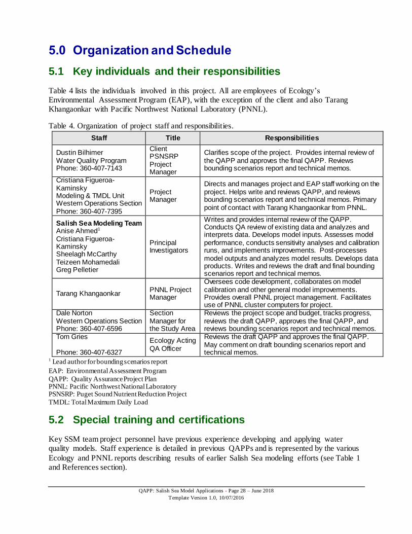
5.1 Key individuals and their responsibilities
Table 4 lists the individuals involved in this project. All are employees of Ecology’s Environmental Assessment Program (EAP), with the exception of the client and also Tarang Khangaonkar with Pacific Northwest National Laboratory (PNNL).
Table 4. Organization of project staff and responsibilities.
Staff Title Responsibilities
Dustin Bilhimer Water Quality Program Phone: 360-407-7143
Client PSNSRP Project Manager
Clarifies scope of the project. Provides internal review of the QAPP and approves the final QAPP. Reviews bounding scenarios report and technical memos.
Cristiana Figueroa-Kaminsky Modeling & TMDL Unit Western Operations Section Phone: 360-407-7395
Project Manager
Directs and manages project and EAP staff working on the project. Helps write and reviews QAPP, and reviews bounding scenarios report and technical memos. Primary point of contact with Tarang Khangaonkar from PNNL.
Salish Sea Modeling Team Anise Ahmed1
Cristiana Figueroa-Kaminsky Sheelagh McCarthy Teizeen Mohamedali Greg Pelletier
Principal Investigators
Writes and provides internal review of the QAPP. Conducts QA review of existing data and analyzes and interprets data. Develops model inputs. Assesses model performance, conducts sensitivity analyses and calibration runs, and implements improvements. Post-processes model outputs and analyzes model results. Develops data products. Writes and reviews the draft and final bounding scenarios report and technical memos.
Tarang Khangaonkar PNNL Project Manager
Oversees code development, collaborates on model calibration and other general model improvements. Provides overall PNNL project management. Facilitates use of PNNL cluster computers for project.
Dale Norton Western Operations Section Phone: 360-407-6596
Section Manager for the Study Area
Reviews the project scope and budget, tracks progress, reviews the draft QAPP, approves the final QAPP, and reviews bounding scenarios report and technical memos.
Tom Gries Phone: 360-407-6327
Ecology Acting QA Officer
Reviews the draft QAPP and approves the final QAPP. May comment on draft bounding scenarios report and technical memos.
1 Lead author for bounding scenarios report
EAP: Environmental Assessment Program
QAPP: Quality Assurance Project Plan PNNL: Pacific Northwest National Laboratory PSNSRP: Puget Sound Nutrient Reduction Project
TMDL: Total Maximum Daily Load
5.2 Special training and certifications
Key SSM team project personnel have previous experience developing and applying water quality models. Staff experience is detailed in previous QAPPs and is represented by the various
Ecology and PNNL reports describing results of earlier Salish Sea modeling efforts (see Table 1 and References section).

QAPP: Salish Sea Model Applications - Page 29 – June 2018
Template Version 1.0, 10/07/2016
5.3 Organization chart
Table 4 lists the key individuals, their current position, and their responsibilities for this project.
5.4 Proposed project schedule
Table 5 presents the proposed project schedule for this project. The project schedule depends on the policy process that underlies it and may be subject to changes throughout the duration of this
work. It is a proposed schedule that was developed for scoping purposes. The schedule and data products may change as this project progresses, and may be outside the control of the SSM team.
Table 5. Proposed project schedule for modeling work and written documents for the Puget Sound Nutrient Source Reduction Project (PSNSRP).
Task Expected
Completion
Bounding Scenarios
Work
Modeling effort
Improvements to model calibration and developing model inputs June 2018
Conducting existing and reference conditions runs June 2018
Conducting bounding scenarios runs July 2018
Model output and processing and analysis July 2018
Model performance assessment July 2018
Bounding Scenarios Report (Author Lead: Anise Ahmed)
Draft due for Internal Team/Client Review July 2018
Draft due for External Peer Review August 2018
Revisions for Final Report September 2018
Final to Publications Coordinator September 2018
Final Report due on Web October 2018
Optimization Scenarios
Work
Modeling effort
Improvements to model calibration and developing model inputs Ongoing
Continuing model performance assessment December 2020
Running model scenarios (optimization runs) March 2021
Model output and processing and analysis March 2021
Baseline model support and improvements (meetings and contract management)
December 2021
Communication of Science
Participation in modeling and project group meetings, developing interim data products, creating presentations
December 2022
Technical Memos due December 2022
5.5 Budget and funding
This work for SSM applications and modeling scenarios may be partially funded by National
Estuary Program (NEP) grants among other resources. The totals do not include costs for some Ecology staff time funded through other state or federal sources.

QAPP: Salish Sea Model Applications - Page 30 – June 2018
Template Version 1.0, 10/07/2016
Table 6. Proposed budget and funding for modeling work for the Puget Sound Nutrient Reduction Project (PSNSRP).
Category Deliverable Group Estimated
Cost Estimated Schedule
Modeling and Technical work to support PSNSRP
SSM bounding scenarios EAP-MTU Funded 2018
SSM optimization scenarios EAP-MTU Funded 2018-2021
PNNL Continuing SSM Development and Collaboration FY 2018
PNNL
Funded FY2018
PNNL Continuing SSM Development and Support FY 2019
$110,000 FY2019
PNNL Continuing SSM Development and Support FY 2020-FY21
$182,500 FY2020- Mar 31, 2021
MATLAB software licensing EAP-MTU/WQP
$20,000 3 yrs for user license
Model Requirements
SSM QAPP EAP-MTU Funded 2018
EAP participation with PSNSRP and related projects
EAP-MTU participation on SSM subgroup
EAP-MTU Funded 2018-2022
EAP: Environmental Assessment Program. FY: Fiscal Year.
MTU: Modeling & TMDL Unit. PNNL: Pacific. Northwest National Laboratory. PSNSRP: Puget Sound Nutrient Reduction Project.
QAPP: Quality Assurance Project Plan. SSM: Salish Sea Model.

QAPP: Salish Sea Model Applications - Page 31 – June 2018
Template Version 1.0, 10/07/2016
6.0 Quality Objectives
6.1 Data quality objectives
The Salish Sea Model (SSM) will be used in applications that include implementable options for nutrient reduction from point and nonpoint nutrient sources in Washington State. The objectives of the model scenarios can vary, based on the specific policy questions that preceded the
investigation. For this reason, the primary data quality objective is to accurately characterize and assess model performance, as compared to observations, so that policy and decision makers can take model uncertainty into account when using model output.
6.2 Measurement quality objectives
Not applicable; no field measurements are included.
6.3 Acceptance criteria for quality of data
Best available information from sources such as Ecology, National Oceanic and Atmospheric Administration (NOAA), King County, and University of Washington (UW) is used for model calibration and comparison with model results. Data used for model calibration will be acceptable if they are obtained from credible sources that document and implement their own
respective QA procedures in a QAPP or other equivalent QA document. Data will follow Ecology’s credible data policy (Ecology, 2006). This QAPP does not address the QA procedures for any individual data set collection, but does
reference their respective QAPPs and QA information for existing data sets. Appendix A includes a table with further details describing information and data needed for this work, including website links to data sources.
However, additional sources of information may be considered as needed or as new sources are identified. Any additional sources of data and information used will be included in the final published documents. The process to determine acceptance of additional existing data or data that will be generated during the duration of the multi-year PSNSRP will follow the same criteria
described by Sackmann (2009 and 2011) that was used in previous model versions and applications. These data acceptance criteria include:
Data Reasonableness. Data quality of existing data will be evaluated where available. Best professional judgement will be used to identify erroneous or outlier data, and these data will
be removed from the data set.
Data Representativeness. Data used will be reasonably complete and representative of the location or time period under consideration. Representativeness is a qualitative measure of the degree to which data accurately and precisely represent a characteristic of a population
(EPA, 2012). Incomplete data sets will be used if they are considered representative of conditions during the period of interest. Data from outside the period of interest will be used only if no other data are available. In this case, best professional judgement will be used to determine the utility of the available data.

QAPP: Salish Sea Model Applications - Page 32 – June 2018
Template Version 1.0, 10/07/2016
Data Comparability. Long-term water quality monitoring programs often collect, handle, preserve, and analyze samples using methodologies that evolve over time. Best professional
judgement will be used to determine whether or if data sets can be compared. The report or technical memos will detail any caveats or assumptions that were made when using data collected from differing sampling or analysis techniques.
Continuous data
Continuous data are available at certain sites with data loggers that record monitoring data for various parameters at specific time-intervals (e.g. 30 minutes) for an extended duration. Continuous data are used in a quantitative manner to compare to model output, if the data meet quality standards for the intended application.
For continuous data collected by Ecology, data must go through data verification and adjustment QA/QC procedures. These data checks may be performed in the field and then again during the review process or as needed to adjust data. These data checks include reviewing instrument
function and possible malfunctions, reviewing residuals and adjusting data as appropriate using a weight-of-evidence approach, and using best professional judgement and visual review to confirm any adjustments. These QA/QC procedures for continuous data are described in more detail in each project-specific QAPP, as well as in the Programmatic QAPP (McCarthy and
Mathieu, 2017) and in related standard operating procedures (SOPs). Agencies and organizations outside of Ecology have their own specific QA/QC procedures that they follow to assess the quality of their continuous data and measurement procedures. These
QA/QC procedures may be accessed online with the data (see Appendix A, Table A-1, “Links to QA Information”). Ecology staff will continue to assess and review all continuous data quality based on relevant
data usability assessments, comparability with other observations, other data sources, and professional judgement. If questions about the quality of the data or potential data qualifiers arise, then contacting the sources of the data for verification and further information may be necessary. Any suspect data from point sources will be checked by contacting the appropriate
permit manager for the site. Data that are suspect without sufficient documented QA/QC information will be discarded and not used.
Missing data and data gaps
Due to the large amount of data and sources for data used in this work, missing data and data
gaps will be encountered. Missing data will be addressed using different approaches depending on the intended use of the data. In addition to nitrogen, organic carbon is also a key nutrient that influences DO levels and
acidification in Puget Sound. However, availability of organic carbon data are more limited than nitrogen data. Observations of organic carbon entering Puget Sound are more abundant from point sources, in the form of biological oxygen demand (BOD) measurements, however organic carbon data from the water column in either rivers or streams marine waters are sparse. A
component of the ongoing work for this study involves reviewing organic carbon data that pertains to the Puget Sound region, as it becomes available, such as recent work from the USGS that monitored organic carbon in the Green and Duwamish Rivers (Conn et al., 2018).

QAPP: Salish Sea Model Applications - Page 33 – June 2018
Template Version 1.0, 10/07/2016
For data used in model inputs (e.g. river flows, water quality), missing data from time series will be estimated. This is necessary to ensure that the model inputs contain comprehensive information to represent the conditions of water quality and physical processes in the Salish Sea.
For small data gaps (e.g. a daily value), the missing data will be estimated based on linear interpolation.
For larger data gaps (e.g. multiple consecutive weeks of missing data), regressions will be
created based on existing data and extrapolated to account for data gaps to be used in the model input to ensure that there are sufficient data for the entire modeling duration. Extrapolation approaches will be reviewed by computing descriptive statistics upon comparing results with known data. Extrapolation approaches that provide optimal statistics
(highest accuracy, lowest error, and bias), and for which data sets are available, will be used.
6.4 Model quality objectives
Previous calibrations of the SSM have been documented in previous reports and work (see Section 3.2.2). This work will use previously calibrated versions of the SSM for water quality conditions scenarios and model applications. If needed, the process for model re-calibration is
described in Section 13.4. To meet project goals and objectives, model quality results should be similar to observations, modeling results in previous SSM work, and other models used in similar Salish Sea modeling
projects and reports. Model performance measures the ability of a model to reproduce characteristics in the processes and parameters being simulated. Model performance for these results will be evaluated through quality assessment procedures (Section 13.4). The bounding scenarios report and technical memos will summarize model performance, describe how model
performance affects the interpretation and uncertainty of the results, and recommend next steps that could include management actions or further projects. Indicators of model quality include the following considerations:
Goodness-of-fit: The accuracy with which the model is able to predict observed data. This can be described through bias and by visually comparing plots of modeled and observed values.
Accurate representation of processes: The modeling results should achieve reasonable
predictions by invoking correct explanations of observed data and reasonably simulating real-world processes.
Sensitivity to key inputs: The model should be able to reasonably predict the response of the system to key inputs.

QAPP: Salish Sea Model Applications - Page 34 – June 2018
Template Version 1.0, 10/07/2016
7.0 Study Design
7.1 Study boundaries
The study boundaries are defined by the model domain for the SSM and include areas in the U.S.
and Canada. The model domain encompasses the Salish Sea (Puget Sound, Strait of Georgia, and Strait of Juan de Fuca), in addition to a section along the Pacific Coast out to the continental shelf (Figure 6).
There are currently two versions of the model: (1) the original version Puget Sound Model (PSM) and (2) an updated version Salish Sea Model (SSM). The original PSM model domain extended from the mouth of the Strait of Juan de Fuca to South Puget Sound. The northern boundary was set at the entrance to Johnstone Straits past the Fraser River north of Vancouver
B.C. The model grid was expanded from the model domain used in previous studies to the continental shelf to improve circulation modeling of the entire Salish Sea (Khangaonkar and Xu, 2017). The expanded grid model now includes Discovery Islands, Johnstone Strait, Broughton Archipelago and the associated waterways, along with major rivers along the Pacific Coast
(Chehalis, Columbia, Willamette, and Willapa Rivers) (Figure 6).
Figure 6. Salish Sea Model expanded grid model domain.
More descriptions for the study boundaries can be found in Sackmann (2009) and Khangaonkar
and Xu (2017).

QAPP: Salish Sea Model Applications - Page 35 – June 2018
Template Version 1.0, 10/07/2016
7.2 Field data collection
This QAPP addresses the QA procedures for using the SSM in model applications. Data from additional field studies may be used to help refine model inputs and as comparisons with model results. Any additional field work will have its own project-specific QAPP outlining field
collection procedures and data quality objectives.
7.3 Modeling and analysis design
7.3.1 Model setup and data needs
SSM is a complex, 3-D model used to simulate hydrodynamics and water quality using an unstructured grid framework. The model has been updated and improved, resulting in different
versions of the Salish Sea Model (PSM and SSM). A summary of the various versions of the SSM and its related hydrodynamic model, water quality model, and ocean boundary setup are presented in Table 7. Details for these previous model setups are found in Appendix B and in previous model documents (Sackmann 2009; Khangaonkar et al., 2012a,b; Khangaonkar et al.,
2011; Yang et al., 2010).
Table 7. Salish Sea model versions.
Version
Year
Initially
Calibrated
Brief description Ocean Boundary
PSM0 2012 Original intermediate-scale model Strait of Juan de Fuca
& Johnston Strait
PSM1 2016 Intermediate-scale model with sediment diagenesis. Strait of Juan de Fuca & Johnston Strait
PSM2 2016 Intermediate scale model with sediment diagenesis and ocean acidification.
Strait of Juan de Fuca & Johnston Strait
SSM0 2017 Expanded grid, intermediate scale model with
sediment diagenesis and ocean acidification. WA continental shelf
SSM1 2018 Expanded grid, intermediate scale model with sediment diagenesis and ocean acidification,
refined and distributed freshwater inflows.
WA continental shelf
SSM2 2018
Expanded grid, intermediate-scale model with SD
and OA, refined and distributed freshwater inflows
plus Canadian watersheds
WA continental shelf
SD: Sediment diagenesis
OA: Ocean acidification

QAPP: Salish Sea Model Applications - Page 36 – June 2018
Template Version 1.0, 10/07/2016
This project describes the model setup and data needs for the current version of the SSM (SSM2). Earlier versions of the model (e.g. PSM2) may be applied to simulate water quality conditions in the Salish Sea. These will be as determined necessary by the modeling team, due to
the benefits of earlier model versions, such as lower associated costs due to shorter model run time. Table 8 presents a summary of the data needs for both the hydrodynamic and biogeochemical
water quality component of the model. Appendix A includes a table with specific sources and descriptions for each of the types of data used in the model.
Table 8. Summary of data needs for model inputs for the hydrodynamic and water quality model.
Model Inputs/Results Data Needs
Hydrodynamic Model – Model Input
Freshwater flows for river and stream inflows
Freshwater temperature data
Atmospheric and meteorological data
Marine point sources discharge
Tides and water surface elevation data
Water Quality Model – Model Input
Freshwater quality data for river and stream inflows
Marine water quality data at ocean boundary
Marine point sources water quality data
Model Results Comparison
Marine water observations (temperature, salinity)
Marine water quality data
Tides and water surface elevation data
The hydrodynamic component of the SSM is an application of the unstructured grid Finite-
Volume Community Ocean Model (FVCOM; Chen et al., 2003). The unstructured grid framework allows for the representation of complex shoreline geometry, waterways, and islands in the Salish Sea. FVCOM can simulate wetting and drying and uses a sigma grid system where the vertical layer thickness changes to simulate sea surface height.
The biogeochemical component is an adaptation of the Integrated Compartment Model (CE-QUAL-ICM; Cerco and Cole, 1995), which is referred to as FVCOM-ICM when coupled with the FVCOM hydrodynamic model (Kim and Khangaonkar, 2010). FVCOM-ICM is run non-
concurrently and uses hydrodynamic fields computed by FVCOM using the model grid. Both of these modeling frameworks, including equations used to represent physical, biological, and chemical processes, have been documented and used extensively in other peer-reviewed studies (Chen et al., 2003; Khangaonkar et al., 2011, 2012, 2018; Kim and Khangaonkar, 2012; Pelletier
et al., 2017a,b; Bianucci et al., 2018). A schematic diagram represents the biogeochemical processes and key parameters included in the model (Figure 7).

QAPP: Salish Sea Model Applications - Page 37 – June 2018
Template Version 1.0, 10/07/2016
Figure 7. Biogeochemical processes diagram for the Salish Sea Model (Pelletier et al., 2017b)
The hydrodynamic framework and the model development and testing approach for the original model, including both the circulation and water quality model components, are described in detail by Sackmann (2009 and 2011). These publications provide additional information on
ocean boundary conditions, meteorology, river inputs, marine discharges from WWTPs, and marine profiles and time series for model performance assessment as conducted in prior years. Any updates to methodologies are detailed in Section 7.3.2. The Sediment Diagenesis and Ocean Acidification Modules framework are described in detail by Roberts et al. (2015a,b) and Pelletier
et al. (2017a,b). These publications for previous versions of the model and other related work are presented in the publications table (Table 1, Section 3.2.2). The SSM has a suite of parameters, including rates and constants, used to model hydrodynamic
and biogeochemical processes. Through a series of model enhancements, more parameters have been included in the modeling framework, particularly within the water quality component. The QAPPs and final reports for the Sediment Diagenesis and Ocean Acidification Modules document the parameters added for these modules (Roberts et al., 2015a,b; Pelletier et al.,
2017a,b). The values used for the parameters in the SSM are determined through a combination of review of available, relevant literature and a period of extensive model calibration. An overview of the
types of parameters currently in use are provided below. Calibration parameters may be adjusted to improve model performance. More information about these parameters can be found in Appendix C.
Phytoplankton (diatoms and dinoflagellates): growth rate, photosynthetic rate, metabolic rate,
predation rate, nitrogen-to-carbon ratio, carbon-to-chlorophyll ratio, optimal growth temperature.

QAPP: Salish Sea Model Applications - Page 38 – June 2018
Template Version 1.0, 10/07/2016
Mineralization: nitrification rate, reaeration coefficient, oxygen-to-carbon mass ratio in production and respiration.
Settling: settling rates of fixed solids, labile particulate organic solids, refractory particulate organic matter, diatoms, and dinoflagellates.
Sediment diagenesis: diffusion and advection rate between water and sediment, decay rate of various forms of particulate organic matter, sedimentation, and resuspension rates.
The majority of parameter values for the SSM are commonly accepted to be the same constant values across a large number of studies (e.g., Martin and Wool, 2013; Di Toro, 2001; and Testa et al., 2013). The parameter values were determined through a process of extensive model
calibration, as described in Section 13 and other previous SSM related documents. The range of values for water column parameters that were used for model simulations are documented in Appendix C. These parameter values may be updated, as data sets and more information become available that help to better describe and quantify any of the parameters discussed above.
The Excel formulation of CO2SYS (Pelletier et al., 2015), after the work of Lewis and Wallace (1998), will be used in model setup and testing. CO2SYS is used as a calculator for the carbon dioxide system in seawater written in Microsoft Excel/VBA. This program uses any two
parameters of the carbon dioxide system in seawater (alkalinity, total organic carbon, pH, and fugacity or partial pressure of carbon dioxide), and calculates the other two parameters for given input and output conditions of temperature and pressure. Calcium solubility is also calculated for both calcite and aragonite.
7.3.2 Boundary conditions
Ocean Conditions
The Salish Sea has a continuous open boundary with the Pacific Ocean across the length of the
continental shelf. Water quality conditions were characterized at these open boundaries using available marine water quality data collected either by Fisheries and Oceans Canada (DFO) or jointly by Ecology and UW as part of the Joint Effort to Monitor the Strait of Juan de Fuca (JEMS). Data from NOAA’s World Ocean Atlas may be used as needed to supplement data from
DFO and JEMS. Details on how data were used to create open ocean boundary conditions and uncertainties at this boundary are described by Khangaonkar et al. (2017, 2018). An area of continued research to improve modeling at the open ocean boundary includes the use
of global ocean models, such as HYCOM (Halliwell et al., 1998, 2000; Bleck, 2002) as inputs. The ocean boundary methodology is expected to be updated as new scripting and modeling tools are developed that are able to utilize these global models. Particularly, this will become necessary when modeling future years based on the Intergovernmental Panel on Climate Change
(IPCC) climate change scenarios. An addendum to this QAPP will be written to specify details for climate change runs.
Meteorology
Meteorological boundary conditions are required to simulate circulation and water quality. These
include wind speed and direction, heat flux, irradiance, and day length. Meteorological data are used in both the hydrodynamic (FVCOM) and water quality (CE-QUAL-ICM) model

QAPP: Salish Sea Model Applications - Page 39 – June 2018
Template Version 1.0, 10/07/2016
framework. The original SSM (PSM0-1) used the North American Regional Reanalysis data sets from NOAA (Yang et al., 2010) on a 30 km x 30 km grid. An overwater station near the triple junction at the south end of Whidbey Island near the center of Puget Sound was also previously
used to calculate representative net heat flux applied to the entire domain. These data were available on a 6-hourly interval basis. Meteorological inputs for the SSM were improved by transitioning to the Weather Research
Forecasting (WRF) model reanalysis data provided by the UW on a finer resolution, 12 km x 12 km grid (Khangaonkar et al., 2012a). These are hourly data. The WRF Model, as implemented by the Northwest Regional Modeling Consortium, provides an increased resolution of distributed wind, air temperature, and other meteorological data over the Puget Sound region. These data
have been available since 2009. Meteorological data for previous years is also available from the Northwest Regional Modeling Consortium but from MM5 (fifth generation Penn State/ National Center for Atmospheric Research Mesoscale Model).
For future years and climate change scenarios, data will be dynamically down-scaled global from model scenario predictions. An example of this type of work using down-scaled global models is in the climate change scenarios report by Khangaonkar et al. (2018a).
WRF model reanalysis data are also available from the UW on a finer resolution, 4 km x 4 km grid. This allows for more WRF nodes within the Salish Sea, but more importantly within Puget Sound. Future model scenarios may use a hybrid approach with WRF data from both grids. Data from the coarser grid (12 km x 12 km grid) will be used for Washington and Canadian coastal
waters and the Straits of Juan De Fuca and Georgia, while data for Puget Sound may be used from the finer grid (4 km x 4 km grid).
Watershed Inflows
Watershed inflows into the model domain include freshwater into Puget Sound, the Strait of
Georgia, and the Strait of Juan de Fuca as well as Johnstone Strait and major river inflows into the Pacific Ocean. These freshwater inflows include large rivers, smaller streams, unmonitored watersheds, and the shoreline fringe. Previous versions of the SSM included estimates of flow and nutrient concentrations at a daily interval from 64 freshwater inflows. The methods used to
develop these are summarized in Mohamedali et al. (2011). The original 1999-2008 time-series of flow estimates used in previous SSM versions have been updated with newer and additional data to account for more recent flow values. These flow
estimates now also accommodate the greater number of inflows needed for the expanded and refined versions of the model grid. These changes and updates include:
There are now 161 freshwater inflows entering the model domain. These additional freshwater inflows are mostly a result of:
o Subdividing larger watersheds from previous model versions into smaller watersheds. The improvement in the spatial resolution of watershed inflows was primarily focused on watersheds in South and Central Puget Sound.

QAPP: Salish Sea Model Applications - Page 40 – June 2018
Template Version 1.0, 10/07/2016
o Adding the larger rivers that discharge into the Pacific Ocean of Washington State since these rivers are now within the expanded model boundary which includes the Washington coastline.
o Adding flow from Canadian watersheds that drain into Johnston Strait and the Strait of Georgia which are now within the northern portion of the expanded model boundary.
The methods for flow estimates were kept consistent with those described by Mohamedali et
al. (2011), where streamflow data were normalized and scaled (by drainage area and average annual precipitation of each watershed) to estimate flow from ungaged watersheds (or ungaged portions of the watershed). However, the average annual precipitation for each watershed was updated and now uses ‘PRISM 30-year Normals’ which cover the period
1981-2010. The modeling team is evaluating the use of WRF-Hydro and may implement its use for hydrological flow estimates.
The flow time series was extended beyond 2008 to include flow estimates from 2009-2017 for all freshwater inflows.
Flow estimates for the Green River were updated by scaling flow values from USGS’s Green River near Auburn site (Station No. 12113000).
Flows to represent Lake Washington and Ballard Locks were updated. Previously, this had been estimated using a combination of upstream gages. The updated flow is now based on actual flow measurements taken by the US Army Corps of Engineers near Ballard Locks from 2006-2017.
A new inflow was added to capture the flow from ‘Cushman Powerhouse No. 2’. This is a
diversion of flow, monitored by Tacoma Public Utilities, that is located below Lake Kokanee and goes through a Powerhouse and then is discharged into Hood Canal. This inflow was previously missing.
Flow estimates are now based on 39 stations with long-term streamflow gage data. Most of the gages used in Washington State are maintained and run by the USGS, but those on the Canadian side are maintained and run by the Government of Canada.
Estimates of time-varying water quality data were also developed by Mohamedali et al. (2011) for 1999-2008. These were based on a statistical method called multiple-linear regression, which related concentrations to flow and time of year using a best fit to monitoring data. The methods and regression coefficients for water quality estimates are kept consistent, but the following
changes and updates have been made:
The time-series of water quality parameters was extended beyond 2008 to include 2009-2017.
Alkalinity and pH estimates were added for every inflow based on available data, since these
estimates were needed for the acidification module of the model (Pelletier et al, 2017b; Bianucci et al., 2018).
The extension of the time-series for water quality data used the original multiple linear
regressions that were developed based on data primarily collected in 2006-2007. As part of upcoming work, the regression predicted water quality variables will be compared with

QAPP: Salish Sea Model Applications - Page 41 – June 2018
Template Version 1.0, 10/07/2016
observations where data are available (e.g. at Ecology freshwater ambient monitoring stations where we have monthly data for each year for the major rivers entering Puget Sound). This will help to validate whether the original multiple linear regression parameters are still relevant for
2009-2017, or if they need to be revised in order to refine the estimates. Reference conditions (previously referred to as ‘natural conditions’) for these watershed inflows were also estimated by Mohamedali et al. (2011), including natural DIN concentrations and
loads in the absence of human influence. These were updated to also include estimates of organic nitrogen and organic carbon reference conditions as described in Pelletier et al. (2017b). The difference between existing and reference conditions represents our best estimate of human nutrient contributions within watershed inflows. Human contributions from watershed sources
include the combined effects of point and nonpoint sources. The methods used to calculate reference conditions may be reviewed again for future model use and may be updated with additional data or improved methods if better information is available. Any changes to the reference conditions will be documented in the bounding scenarios report or technical memos.
For future year and climate change scenarios, watershed hydrology inputs will be adapted from future climatic conditions based on available simulations. Oceanographic and meteorological data for future conditions will be developed by downscaling global scale model outputs
(Khangaonkar et al., 2018a).
Marine Point Sources
‘Marine point sources’ refers to the 99 municipal WWTPs and industrial facilities that discharge directly into Puget Sound, the Strait of Georgia, and the Strait of Juan de Fuca, and are included
in the current version of the model. This includes WWTPs located in the U.S. and Canada, oil refineries, active pulp and paper mills, and an aluminum facility. Additional point sources discharge further upstream in rivers that reach the Salish Sea. These sources are not individually quantified, but their contributions are included in the watershed inflow estimates.
Marine point sources are represented as discrete points that enter into the model domain at specified nodes. For this version of the model, the point source plume enters at a specified layer within the water column at the plume trapping depth estimated externally with mixing zone
models. PNNL is in the process of developing a tool to simulate effluent dilution and mixing from outfalls within the SSM. Depending on the demonstration of performance of this tool, the modeling team may use it during the optimization runs.
Flow and water quality loading estimates were originally estimated at daily intervals for these point sources from 1999-2008, as described in Mohamedali et al. (2011). This approach used a combination of plant-specific data (where available) and template concentration values based on plant size. Plant specific flow and water quality data for several parameters were acquired from
discharge monitoring reports and focused monitoring efforts in 2006-2007. Where sufficient data exists, plant-specific regressions were developed for those parameters (mostly carbonaceous biochemical oxygen demand and ammonium). Available concentration
data were then analyzed to develop concentrations templates by facility size (large plants > 10 mgd, medium plants 4-10 mgd, small plants < 4 mgd). Template concentrations were applied to those facilities for which there was no site-specific water quality data. Most large facilities had

QAPP: Salish Sea Model Applications - Page 42 – June 2018
Template Version 1.0, 10/07/2016
plant-specific water quality information and did not use template values. Plant-specific flows were used to generate loads. For industrial facilities, characteristic concentrations were developed using best available
information for the pulp and paper mills, oil refineries, and an aluminum facility. Plant-specific data for Canadian WWTPs were used where available. Because Canadian WWTPs are not the focus of the study and data are limited, often a single year-round concentrations value is applied for each month of the year based on the treatment levels at each plant.
The main updates to marine point source inflows since Mohamedali et al. (2011) include:
Extending the flow and water quality time-series beyond 2008 to include 2009-2017.
Acquiring updated water quality data from discharge monitoring reports for more facilities, and developing plant-specific regressions for these instead of using the template concentrations. This included updated information on Canadian WWTPs from Metro Vancouver and Capital Regional District Annual reports and personal communication, as
well as new information on federal facilities obtained from EPA.
Including new point sources with data that are now available on a website (e.g. King County’s Brightwater WWTP).
For WWTP where plant unit processes changed, new regressions were developed for missing
data from the time the new unit processes came on line. Old regressions were used for missing data before the unit process change.
Updating model grid nodes to be assigned to all WWTP for the expanded SSM grid. Where
an outfall location changed, a new model grid node was assigned to the new outfall.
7.3.3 Conducting model runs
Modeling work for PSNSRP involves specific modeling scenarios. These are outlined in Section 4.2.1 and apply the SSM in three phases:
1. Modeling current conditions for select years and reference conditions.
2. Conducting bounding scenarios model runs.
3. Conducting optimization scenarios model runs.
Current conditions are determined through hindcasting of recent years, where the model is tested against past observed conditions to assess model performance (CREM, 2009). The years selected to simulate current conditions of the Salish Sea for the bounding scenarios report (2006, 2008) were based on a combination of data availability, model performance, and conditions that are
representative of Puget Sound. For further analyses, additional years may be selected based on data availability and model performance. The year 2006 has been well-studied and documented in various research and modeling
publications as a year that is representative of low oxygen conditions in Puget Sound (Albertson et al., 2016; Khangaonkar et al., 2011 and 2012; Roberts et al., 2014a; Pelletier et al., 2017a,b). 2008 represents a year with more typical conditions in Puget Sound. Figure 8 (Albertson et al., 2016) displays the residence time index for the summer months from 1999-2014. The residence
time index was estimated by a Knudsen relationship using river flow and observational marine data for the upper 30 meters (Albertson et al., 2016; Knudsen, 1900). Residence time is

QAPP: Salish Sea Model Applications - Page 43 – June 2018
Template Version 1.0, 10/07/2016
displayed as an index relative to a 16-year baseline. Note that the index of residence time relative to normal for 2006 is approximately 1.5, whereas during 2008 the index is much closer to zero. Years with higher residence times are typically due to warm, dry conditions and are represented
by higher indices.
Figure 8. Residence time index for the Central Puget Sound basin during summer months, (Albertson et al., 2016).
Reference conditions (referred to as ‘natural conditions’ in previous SSM publications) consist of model runs that are the same as current conditions, except with estimated regional anthropogenic nutrient sources excluded. The effect of regional anthropogenic nutrient sources on water quality will be evaluated by analyzing the difference in results between current conditions and reference
conditions (Mohamedali et al., 2011; Pelletier et al., 2017b). Regional anthropogenic nutrient sources that will be excluded in the reference conditions include the anthropogenic component of loading in the WWTPs, and all freshwater sources will be set to reference condition levels for nitrogen and organic carbon. The bounding scenarios report and technical memos will document
how reference conditions were calculated. After modeling current and reference conditions, the next phase will involve conducting the bounding scenarios runs. These bounding scenarios represent the range of response of water
quality in Puget Sound (both high and low) to major changes in model inputs. These scenarios will improve understanding of the relative importance of these changes and the relative influence of watershed sources compared to marine point sources.
The final phase of modeling runs will involve running the optimization scenarios. These will evaluate different combinations of marine and watershed source reductions that are scaled back from the bounding scenarios to represent different combinations of implementation approaches. Modeling runs will be conducted that simulate the response of the system to nutrient reductions
at different levels and from different sources. To identify the necessary scenarios, these

QAPP: Salish Sea Model Applications - Page 44 – June 2018
Template Version 1.0, 10/07/2016
optimization scenarios will be determined based on continuous discussions and collaboration with the PSNSRP steering committee, Puget Sound Nutrient Forum, Marine WQ Implementation Strategy team, and the SSM team.
7.4 Assumptions in relation to objectives and study area
Modeling work contains inherent assumptions when representing a water body through a simplified mathematical-representation that is not able to fully account for each variable and element influencing the system.
General modeling assumptions for the SSM include:
Equations that are used in the model are representative of the biological, physical, and chemical processes in the Salish Sea.
Rates and constants are reasonable and within literature-reported values, when available.
Marine data that are used for model calibration are representative of the spatial and temporal variation within the Salish Sea.
Watershed inflow data that are used for model calibration are representative of those sources.
Meteorological data derived from model predictions are representative of actual conditions.
Unknown or unidentified sources have a negligible effect on model results.
Vertical distortion from smoothed bathymetry is appropriate at the scales being used in each model version.
The use of downscaled oceanographic and meteorological global models for simulating current or future conditions are representative of the Salish Sea.
Additional modeling assumptions related to river and WWTP loading are documented in Mohamedali et al. (2011). More specific modeling assumptions for the ocean acidification module are described by Long et al. (2014) and Pelletier et al. (2017b). Modeling assumptions
related to the sediment diagenesis module are found in Martin and Wool (2013), Di Toro (2001), and Pelletier et al. (2017a).
7.5 Possible challenges and contingencies
7.5.1 Logistical problems
This project is not expecting any logistical problems, such as field work issues or property access. We have access to all appropriate modeling software.
7.5.2 Practical constraints
Computational requirements and constraints, such as unmet data needs or unknown data quality, are described in Sections 4.3, 11, and 13. Budget constraints may influence the model version
and model runs used for various modeling scenarios. All documentation of model results will describe the model version used. Outside of the modeling work, budget constraints can also influence the amount of data that is able to be collected and used for model input and comparison with model results.

QAPP: Salish Sea Model Applications - Page 45 – June 2018
Template Version 1.0, 10/07/2016
7.5.3 Schedule limitations
Any unforeseen limitations, such as policy challenges, that would affect the project schedule will
be discussed with the modeling team, project manager, and appropriate personnel, as needed, and documented. Schedule constraints that are influenced by modeling work and run-time (see above), may require using a previous version of the SSM for modeling run-time efficiency.
8.0 Field Procedures
Not applicable; no sampling is planned.
8.1 Invasive species evaluation
Not applicable; no sampling is planned.
8.2 Measurement and sampling procedures
Not applicable; no sampling or laboratory analysis is planned.
8.3 Containers, preservation methods, holding times
Not applicable; no sampling or laboratory analysis is planned.
8.4 Equipment decontamination
Not applicable; no sampling or laboratory analysis is planned.
8.5 Sample ID
Not applicable; no sampling or laboratory analysis is planned.
8.6 Chain-of-custody
Not applicable; no sampling or laboratory analysis is planned.
8.7 Field log requirements
Not applicable; no sampling or laboratory analysis is planned.
8.8 Other activities
Not applicable; no sampling or laboratory analysis is planned.

QAPP: Salish Sea Model Applications - Page 46 – June 2018
Template Version 1.0, 10/07/2016
9.0 Laboratory Procedures
Not applicable; no sampling or laboratory analysis is planned.
9.1 Lab procedures table
Not applicable; no sampling or laboratory analysis is planned.
9.2 Sample preparation method(s)
Not applicable; no sampling or laboratory analysis is planned.
9.3 Special method requirements
Not applicable; no sampling or laboratory analysis is planned.
9.4 Laboratories accredited for methods
Not applicable; no sampling or laboratory analysis is planned.
10.0 Quality Control Procedures
10.1 Table of field and laboratory quality control
Not applicable; no sampling or laboratory analysis is planned.
10.2 Corrective action processes
No sampling or laboratory analysis is planned. See Section 7.3 for model setup and testing, and Section 13.4.1 for model calibration and sensitivity testing. Calibration is, by nature, an iterative process that seeks to optimize model performance to a level consistent with understanding of underlying processes and data gaps. Model performance will be evaluated throughout this work,
as will interpreting model output considering uncertainty. If corrective action processes are needed based on the evaluation of model performance and results, project personnel and technical experts will convene to decide on the next steps that need to be taken to improve model performance.

QAPP: Salish Sea Model Applications - Page 47 – June 2018
Template Version 1.0, 10/07/2016
11.0 Data Management Procedures
11.1 Data recording and reporting requirements
Model input and output data for various bounding and optimization scenario runs will be made accessible through different forms, such as varied plots and summary tables, and also via web maps created on Esri’s ArcGIS Online platform. Web maps are developed to display results for
certain model runs and years. Figure 9 is an example of this type of web map that shows existing conditions for annual average DO concentrations in the bottom layer during 2006. These interactive maps allow the user to view specific model output data in geospatial form by selecting various layers that contain model results (left side of Figure 9).
Figure 9. Example of an ArcGIS Online web map that shows model output for existing conditions for annual average DO in bottom layer during 2006.
11.2 Laboratory data package requirements
Not applicable; no sampling or laboratory analysis is planned.
11.3 Electronic transfer requirements
Not applicable; no sampling or laboratory analysis is planned.

QAPP: Salish Sea Model Applications - Page 48 – June 2018
Template Version 1.0, 10/07/2016
11.4 EIM/STORET data upload procedures
Not applicable; no sampling or laboratory analysis is planned.
11.5 Model information management
The primary models FVCOM and FVCOM-ICM used in this Salish Sea modeling project are public domain research codes that undergo modification and testing as part of model
development (e.g., development and incorporation of the sediment diagenesis kinetics into FVCOM-ICM). All source codes used by Ecology are stored on a server at both Ecology and PNNL. If modifications to source codes are needed, these will be performed by Ecology or PNNL staff with appropriate experience. The process for updating model codes is described in
Section 13.4.1. Any changes to model source codes will are discussed with the modeling team and will be noted in model documents and “readme” files.
11.5.1 Cluster computer data management
Running the model requires use of a high-performance computing (HPC) cluster computer using the Linux operating system. The hydrodynamic model takes approximately 0.5 days for run time. Each year-long water quality model run requires the dedicated use of 4 computing nodes with a total of 96 processors for about 2 days. These time estimates do not include pre- and post-
processing of model input and output. The type of computational platform required for running the model is not supported by Ecology’s Information Technology Services Office (ITSO). Ecology plans to use the PNNL
cluster named “Constance” for this project to perform model runs. Constance is a 300-node, 7200 processor super-computer.
Ecology’s modeling server is a storage area network (SAN) housed in Olympia. The Ecology
server is accessed through remote log-in, and read-write permissions for the SSM directory on the modeling server are only allowed for members of the modeling team. All members of the modeling team also have their own secure folder, restricting access from other users. These permission levels improve the overall security of modeling files and significantly decrease the
chance of unintentional file corruption, mistakes, or loss.
11.5.2 Project input and output files
Running the SSM requires a large amounts of data and pre- and post-processing efforts. Model input files are generated after (1) all data have been determined to meet acceptable criteria and
(2) developing nonpoint and point source inflows have been completed. Users upload the model input files with the associated case names to Constance. Running the model produces large amounts of output data and files requiring post-processing. Model output files are copied from Constance to Ecology servers for further processing. Solution files may be downloaded by
individual users for further visualization.

QAPP: Salish Sea Model Applications - Page 49 – June 2018
Template Version 1.0, 10/07/2016
Modeling input and output files are stored on Ecology’s server. Model input and output files will follow certain naming conventions to maintain an organized and consistent record of files. The model runs will be stored into appropriate folders and are named according to the version of the
model, year of the model run, type of modeling run, and the number of the model iteration. In addition to naming protocols, “readme” files may be created that provide more details for specific model runs, files, and organization. These will be created by members of the modeling
team as determined necessary.
11.5.3 Modeling project folders
Modeling project folders will be organized on the current Ecology modeling server. Figure 10 shows an overview of the general layout of the modeling server’s file management system, with each box representing a folder. Changes may be made to this layout as deemed necessary by the modeling team in order to improve efficiency, organization, and overall suitability to the
project’s needs. The file management will follow this basic structure:
The Boundary Conditions folder will have at least two subfolders:
o Nonpoint sources data and analysis, including files relating to river nutrient loading and
flow data.
o Point source data and analysis, including information such as WWTP data.
Each year (e.g. 2006, 2008) will have its own folder that contains at least two subfolders:
o Water quality (WQ) subfolder that contains model input files and model output files for
the water quality model.
o Hydrodynamics (HYD) subfolder that contains model input files and model output files
for the hydrodynamic model.
The Source Code folder will contain code information for:
o FVCOM code.
o ICM code.
Additionally, “readme” and other guidance files may be used and included in different folders and subfolders to support file organization and management. These files may include information detailing a file directory, information contained in a specific subfolder, sources of
data, and status or progress of a certain task.

QAPP: Salish Sea Model Applications - Page 50 – June 2018
Template Version 1.0, 10/07/2016
Figure 10. Folder and file management structure for the modeling server.
Each box designates a folder that contains related files.

QAPP: Salish Sea Model Applications - Page 51 – June 2018
Template Version 1.0, 10/07/2016
12.0 Audits and Reports
12.1 Field, laboratory, and other audits
The modeling team will meet regularly to review recent progress, evaluate project needs, and revisit next steps to meet project objectives. This provides an internal peer review function. The team will present interim results to appropriate project personnel (e.g. PSNSRP steering
committee, Puget Sound Nutrient Forum, and Marine WQ Implementation Strategy team) at key project junctures. These meetings provide review from external parties on key results and graphics before extensive report writing is completed.
12.2 Responsible personnel
Table 4 lists staff responsibilities. The modeling team collaborates on review of interim results.
12.3 Frequency and distribution of reports
Model results will be communicated through various documents throughout this project. At this point for PSNSRP, there will be one bounding scenarios report, multiple technical memos, and numerous data products that may be used for presentations. Interim results will be evaluated internally and externally as the project progresses; these results may be featured in data products
described in Section 14.3. The bounding scenarios report will be a published, peer-reviewed technical report that includes model results from the bounding scenarios objectives (Section 4.2.1). This report will also
contain any updates to the model such as recalibration processes, updated model inputs, and nutrient loading estimates. The bounding scenarios report will follow Ecology’s Environmental Assessment Program’s (EAP) publication guidelines.
Following the bounding scenarios report, technical memos will document key findings of model results, including results from the optimization scenarios. These technical memos will occur at key project junctures and will include any updates or improvements to the model. These technical memos will follow Ecology’s EAP publications guidelines.
12.4 Responsibility for reports
Tables 4 and 5 list the personnel responsible for the bounding scenarios report and technical memos.

QAPP: Salish Sea Model Applications - Page 52 – June 2018
Template Version 1.0, 10/07/2016
13.0 Data Verification
Data used to calibrate the SSM will be from existing data sources. These data have undergone a data quality assessment process, using the quality objectives described in sections 4.3 and 6.3. Data used for model inputs are assessed to be considered usable for this project.
This section describes the model calibration process and the analysis methods used for assessing model sensitivity and uncertainty.
13.1 Field data verification, requirements, and responsibilities
Not applicable; no sampling or laboratory analysis is planned.
13.2 Laboratory data verification
Not applicable; no sampling or laboratory analysis is planned.
13.3 Validation requirements, if necessary
Not applicable; no sampling or laboratory analysis is planned.
13.4 Model quality assessment
Model performance will be evaluated using quantitative and qualitative methods to determine the relative quality of model calibration and model results (EPA, 2002; CREM, 2009). Model
performance statistics are evaluated using comparisons of model output with observations. Sensitivity and uncertainty analyses will be conducted to assess the variability of the model results to specific parameters and level of confidence in key output values.
13.4.1 Calibration and evaluation
Calibration refers to the process of adjusting model parameters within physically defensible ranges until the resulting predictions give the best possible match with observed data (EPA, 1994). Model evaluation is the process used to determine whether a model and its analytical results are of sufficient quality to serve as the basis for a decision and whether the model is
capable of approximating the real system of interest (EPA, 2002). Some modeling projects refer to this as validation, confirmation, or verification. Model calibration is an iterative procedure that combines quantitative and qualitative comparison
with measured data and best professional judgment. The calibration process is sometimes limited by sparse availability of observational data, which can vary for different parameters. As more acceptable data become available, the opportunity of optimizing or improving model calibration will be considered. This process is important for long-term projects such as this one. Thus, model
calibration can occur throughout the implementation of a model. This optimization process will

QAPP: Salish Sea Model Applications - Page 53 – June 2018
Template Version 1.0, 10/07/2016
be based on a comparison of new model calibrations with model performance results from previous model versions and applications.
An updated model calibration is considered optimized and will be used if the model performs as well as or better than the results from previous model versions regarding key parameters (temperature, salinity, DO, nitrate, pH, or alkalinity), using the same performance evaluation methods, such as root-mean-square-error (RMSE) and bias. The optimally calibrated model will
demonstrate a balanced performance among biogeochemical parameters. This optimally calibrated model will be used to run scenarios for each stage of the project as the model development process improves. Model hindcasting is used to test the model against past observed conditions (CREM, 2009). This project will use this model hindcasting method to
account for current conditions. Calibration and evaluation rely on a combination of quantitative statistics for goodness-of-fit and visual comparison of predicted and observed time series and depth profiles (Krause et al., 2005).
This project will continue to use similar approaches as reported in Sackmann (2009), Roberts et al. (2014a), Ahmed et al. (2014), and Pelletier et al.(2017a,b), as needed. Model performance will be optimized by consulting the modeling team and EPA modeling guidance documents (CREM, 2009; EPA, 2002; EPA, 2016).
Periodic improvements to the model code are possible. Updated parameterization schemes or computational code improvements are expected on a regular basis due to continued research by the broader modeling community and availability of more data. The SSM team may determine
that updates or code modifications are appropriate. Modifications to the model code will be completed by either the SSM team or PNNL staff with appropriate knowledge of the source code.
After any source code modifications, sensitivity runs will be conducted for key parameters and discussed with the modeling group. Model results from modifications to the source code will be summarized and submitted to the modeling team for review and discussion. Once any model code changes have been tested and accepted, they are assessed for model performance. If
appropriate, updates to the underlying equations that represent the biogeochemical phenomena implicit in the model formulation listed in Appendix D will be necessary.
13.4.1.1 Evaluating model performance
Previous efforts have assessed the quality of data used as input or comparison data for SSM
applications. Marine data collected by various entities using appropriate quality controls are used to evaluate accuracy (measured by RMSE) and bias. These include Ecology’s ambient marine monitoring program data, as well as data from special studies such as the South Puget Sound Dissolved Oxygen Study (Roberts et al., 2008). These data have been assessed for quality prior
to publication. Section 4.3 and Appendix A provide more information about acceptable data and sources that may be used during calibration and evaluation of the SSM.

QAPP: Salish Sea Model Applications - Page 54 – June 2018
Template Version 1.0, 10/07/2016
Initially, model results are compared with observational data using scatter plots and other means of basic data visualization. This allows for a qualitative assessment of model performance and a visualization tool for potential bias. Model results are summarized using descriptive statistics
(e.g. mean, maximum, minimum) and compared to observations, when acceptable data are available. Model resolution and performance are measured using the root-mean-square-error (RMSE), a
commonly used measure of model variability (Reckhow, 1986). The RMSE is defined as the square root of the mean of the squared difference between observed and simulated values. RMSE will be used to estimate:
1. Error between model predictions and observations for any given model run or year
(RMSEexisting).
2. Error inherent in the difference between highly correlated model runs, such as a reference
scenario run paired with a hindcast run (RMSEdiff).
Root-Mean-Square-Error Statistic (RMSE). The RMSE (Erms) is defined as
𝐸𝑟𝑚𝑠 = √∑(𝑂 − 𝑃)2
𝑛
where, O = observation
P = model predication at same location and time as the observation n = number of observed-predicted pairs Erms = root-mean-square-error
The following equations (Snedecor and Cochran, 1989) will be used to estimate the variance of the difference between existing conditions and reference conditions (Vardiff ) and the RMSE of these two model runs (and RMSEdiff). These equations use the variance of the existing condition as an estimate of the variance of the reference condition (R is Pearson’s correlation coefficient
between existing and reference conditions):
Varexisting = RMSEexisting2
Varreference = RMSEreference2 = RMSEexisting
2 Vardiff = Varexisting + Varreference – 2 * R * RMSEexisting * RMSEreference RMSEdiff = Vardiff
0.5
In addition to using RMSE to evaluate model performance, this study will evaluate mean bias and may use other statistics to assess model accuracy. While there are no specifications for tolerance values for RMSE or bias, they will be compared with values from other studies and
previous model runs. RMSE and bias will be evaluated for the following parameters: DO, temperature, salinity, carbonate system parameters, chlorophyll, and nutrient profiles plus time series in the surface and bottom layers, when data are available.

QAPP: Salish Sea Model Applications - Page 55 – June 2018
Template Version 1.0, 10/07/2016
Previous model performance statistics for the SSM did not include Padilla Bay, a shallow, tidally influenced mud-flat region in Puget Sound. While the model performs well compared to observational data for some parameters in Padilla Bay related to hydrodynamics (e.g.
temperature), it does not perform as well for other key parameters (e.g. DO, shown in Figure 11). These influential factors include:
The current grid configuration of SSM is not designed to resolve the bathymetry of mud-flat,
intertidal areas at this point.
Eelgrass or other submerged aquatic vegetation-dominated system that causes a significant
difference in terms of DO, pH, and other important ecosystem characteristics in Padilla Bay.
Figure 11. Comparison of model results with observational data for dissolved oxygen (DO) in Padilla Bay.
13.4.2 Sensitivity and uncertainty analyses
Model performance and the variability of results are evaluated through sensitivity and
uncertainty analyses. Uncertainty can arise from a number of sources that range from errors in the input data used to calibrate the model, to imprecise estimates for key parameters, to variations in how processes are parameterized in the model domain. EPA’s Council on Regulatory Environmental Modeling describes how sensitivity and uncertainty analyses are used
to evaluate model performance (CREM, 2009). By estimating the uncertainty associated with parameter values and the sensitivity of the model to specific parameters, a user will be more informed regarding the confidence that can be placed in the model results.
Uncertainty analysis investigates the lack of knowledge about a certain population of the real value of model parameters. Thesecan include either qualitative or quantitative assessments. Qualitative assessments are used when the uncertainty in model predictions may arise from sources whose uncertainty cannot be quantified (CREM, 2009). This requires best professional

QAPP: Salish Sea Model Applications - Page 56 – June 2018
Template Version 1.0, 10/07/2016
judgement from the modeling team to determine appropriate values for model parameters and inputs that cannot be directly observed or measured. Quantitative assessments involve statistical uncertainty and sensitivity analyses.
A main reason for model uncertainty is due to a lack of data that adequately describes the temporal distribution of rates and parameters within the system to be used as a comparison with model results (CREM, 2009). Model uncertainty can be improved through additional data. As
new data at a finer temporal or spatial resolution become available, these data will be included with the comparison of model results. Any new data used to evaluate model performance will meet the acceptance criteria outlined earlier (Section 6.3). These data are determined to be acceptable if they accurately and precisely represent a characteristic of a population (EPA,
2002). Sensitivity analysis measures the effect of changes in input values or assumptions on the outputs (Morgan and Henrion, 1990). In contrast, uncertainty analysis investigates the lack of knowledge
about a certain environmental component or the real value of model parameters. Although sensitivity and uncertainty are closely related, uncertainty is parameter-specific and sensitivity is algorithm-specific with respect to model variables. By investigating the relative sensitivity of model parameters, a user can better understand the relative importance of the interactions of
parameters in the model, based on the modeling framework and setup. Numerous sensitivity tests for SSM were performed as part of calibrations for previous studies which resulted in acceptable model calibration and selection of model coefficients for water
column processes (Roberts et al., 2014a; Khangaonkar et al., 2012b; Pelletier et al., 2017a,b). Prior SSM publications documented sensitivity tests focused on the response of key parameters (e.g. DO, algal carbon, nutrients, pH) to changes in rates, constants, and boundary conditions. Many of these sensitivity analyses were used to characterize how influential several processes
are in terms of DO. Any new updates from model calibration and optimization will require additional sensitivity tests to continuously assess model performance. During the model evaluation process, the sensitivity
of model outputs for key parameters (e.g. temperature, salinity, DO, and nitrate) are evaluated to better understand the magnitudes of responses to perturbations of model input or coefficients. With each model calibration and optimization iteration, model performance is expected to improve.
Additional statistical tests may be used to assess sensitivity and uncertainty of the model and model results. These will be determined, as appropriate, by the modeling team. These methods and results will be included in the final published documents.

QAPP: Salish Sea Model Applications - Page 57 – June 2018
Template Version 1.0, 10/07/2016
14.0 Data Quality (Usability) Assessment
14.1 Process for determining project objectives were met
This QAPP outlines the procedures and methods that help ensure that performance of the model, when used with existing and best available data, will be satisfactory to meet project goals and objectives.
The process for determining if the project’s objectives were met involves evaluating if the SSM:
Behaves in a manner that is consistent with the current understanding of processes known to
affect water quality in the Salish Sea.
Realistically reproduces variations in water quality observed within individual sub-basins of
Puget Sound and the Straits on inter-annual, seasonal, and possibly intra-seasonal timescales.
The modeling team will (1) prepare written documentation addressing the calibrated model’s ability to meet specific project goals and objectives, and (2) summarize model performance in the bounding scenarios report, technical memos, and presentations. If a current conditions modeled run falls short of fully meeting goals and objectives, the modeling team will conduct a
thorough review of the problem and potential corrective actions (e.g., by collecting additional data or modifying model code). The modeling team will also provide an assessment of how it may still be useful for addressing study questions. The modeling team will determine appropriate uses of the SSM based on model performance and
available resources, per consultation with the PSNSRP steering committee on the types of decisions that need to be made. If the modeling team determines that the quality of the model is insufficient to address any aspects of the project goals and study objectives, the modeling team will consult with peers, experts, and partners, as appropriate. This will involve assessing the
levels of uncertainty present in the model, which requirements can be met, and any actions needed to address the issue.
14.2 Treatment of non-detects
Existing data sets from Ecology and other credible sources will be used for model inputs and as data observations to compare with model results. Due to the large volumes of data used for this
project, these data sets may include non-detects. Using non-detects in modeling will be treated in several ways depending on goodness-of-fit. Non-detects may be:
Replaced with half the detection limit.
Replaced with a raw laboratory instrument value.
Treated as an indeterminate value between zero and the detection limit. For example, when comparing model predictions to observed data where the observed data are a non-detect, any predicted value less than the detection limit would be considered a reasonable match.

QAPP: Salish Sea Model Applications - Page 58 – June 2018
Template Version 1.0, 10/07/2016
14.3 Data analysis and presentation methods
A variety of data analysis methods will be used at different stages throughout this study. These methods will be used during the model application process, including as a means to analyze existing data for model input and model output results. Statistical analyses may be performed to
further analyze the data. Some of these data analysis and statistical methods may include:
Regressions to interpolate results for specific times and locations with missing data.
Graphical and tabular forms to show a comparison of observed values with model results.
Descriptive statistics and summary statistics.
Additional statistical analyses, as determined necessary by the modeling team.
Model performance will be evaluated through uncertainty and sensitivity analyses discussed in Section 13.4. Numerous presentation methods will be used to show model results and related data. These
presentation methods may include:
Visual representations of data in the form of planview maps, cross-sections, depth profiles, and three-dimensional projections of different parameters.
Time series of model output at a particular location.
Animations to show model simulation over time.
Tables with quantitative information, including tables of values specific to various scenarios.
Descriptive statistics and summary statistics plots.
Mathematical function plots including regressions.
Informal, unpublished presentations containing data products.
The above approaches may be used during oral presentations, communication, or published materials including maps, graphics and figures, the bounding scenarios report, and technical memos.
14.4 Sampling design evaluation
Not applicable; no sampling or laboratory analysis is planned.
14.5 Documentation of assessment
There will be one bounding scenarios report and multiple technical memos that will document the results for PSNRSP modeling work. In addition, interim findings will be presented at various project steps to key members of the larger project group, such as members of the PSNSRP
steering committee, the Puget Sound Nutrient Forum, and the Marine WQ Implementation Strategy team.

QAPP: Salish Sea Model Applications - Page 59 – June 2018
Template Version 1.0, 10/07/2016
15.0 References
Ahmed, A., G. Pelletier, M. Roberts, and A. Kolosseus. 2014. South Puget Sound Dissolved Oxygen Study: Water Quality Model Calibration and Scenarios. Washington State Department of Ecology, Olympia, WA. Publication No. 14-03-004.
https://fortress.wa.gov/ecy/publications/summarypages/1403004.html. Ahmed, A., G. Pelletier, and M. Roberts. 2017. South Puget Sound flushing times and residual flows. Estuarine, Coastal and Shelf Science. 187.10.1016/j.ecss.2016.12.027.
Albertson, S., C. Krembs, M. Keyzers, L. Hermanson, J. Bos, and C. Maloy. 2016. Puget Sound Marine Waters 2015 Annual Report: Water Quality (IV) water mass characterization. Puget Sound Ecosystem Monitoring Program (PSEMP) Watergroup. 17-18.
Banas, N.S., Conway-Cranos, L., Sutherland, D.A. 2015. Patterns of River Influence and Connectivity Among Subbasins of Puget Sound, with Application to Bacterial and Nutrient Loading Estuaries and Coasts (2015) 38: 735.
Barton, A., B. Hales, G.G. Waldbusser, C. Langdon, and R.A. Feely. 2012. The Pacific oyster, Crassostrea gigas, shows negative correlation to naturally elevated carbon dioxide levels: Implications for near-term ocean acidification effects. Limnology and Oceanography 57: 698-
710. doi: 10.4319/lo.2012.57.3.0698. Bianucci, L., W. Long, T. Khangaonkar, G. Pelletier, A. Ahmed, T. Mohamedali, M. Roberts, and C. Figueroa-Kaminsky. 2018. Elementa: Science of the Anthropocene. Special Feature:
Advances in ocean acidification. Bleck, R., 2002: An oceanic general circulation model framed in hybrid isopycnic-Cartesian coordinates. Ocean Modeling, 4, 55-88.
Brandenberger, J.M., P. Louchouarn, and E.A. Crecelius. 2011. Natural and post-urbanization signatures of hypoxia in two basins of Puget Sound: Historical reconstruction of redox sensitive metals and organic matter inputs. Aquatic Geochemistry.
Cannon, G.A., 1983. An Overview of Circulation in the Puget Sound Estuarine Sys- tem. NOAA Technical Memorandum ERL PMEL-48.
Cerco, C.F. and T.M. Cole. 1995. User’s Guide to the CE-QUAL-ICM Three-Dimensional Eutrophication Model, Release Version 1.0. U.S. Army Corps of Engineers, Washington, DC. 320 pp.

QAPP: Salish Sea Model Applications - Page 60 – June 2018
Template Version 1.0, 10/07/2016
Chan, F., Boehm, A.B., Barth, J.A., Chornesky, E.A., Dickson, A.G., Feely, R.A., Hales, B., Hill, T.M., Hofmann, G., Ianson, D., Klinger, T., Largier, J., Newton, J., Pedersen, T.F., Somero, G.N., Sutula, M., Wakefield, W.W., Waldbusser, G.G., Weisberg, S.B., and Whiteman, E.A. The
West Coast Ocean Acidification and Hypoxia Science Panel: Major Findings, Recommendations, and Actions. California Ocean Science Trust, Oakland, California, USA. April 2016. http://westcoastoah.org/wp-content/uploads/2016/04/OAH-Panel-Key-Findings-Recommendations-and-Actions-4.4.16-FINAL.pdf
Chen, C., H. Liu, R.C. Beardsley, 2003. An unstructured, finite-volume, three-dimensional primitive equation ocean model: Application to coastal ocean and estuaries. Journal of Atmospheric and Oceanic Technology 20:159-186.
Conn, K.E., Black, R.W., Peterson, N.T., Senter, C.A., and Chapman, E.A., 2018. Chemical concentrations in water and suspended sediment, Green River to Lower Duwamish Waterway near Seattle, Washington, 2016–17: U.S. Geological Survey Data Series 1073, 17 p.,
https://doi.org/10.3133/ds1073. CREM, 2009. Guidance on the Development, Evaluation and Application of Environmental Models. Council for Regulatory Environmental Modeling, United States Environmental
Protection Agency. Washington, D.C. Deppe, R.W., J. Thomson, C. Krembs, and B. Polagye, 2013. Hypoxic intrusions to Puget Sound from the Ocean, Oceans. 2013 .MTS/IEEE, San Diego, CA.
Deppe, R.W., J. Thomson, B. Polagye, and C. Krembs. 2017. Predicting deep water intrusions to Puget Sound, WA (USA), and the seasonal modulation of dissolved oxygen. Estuaries and Coasts.
Di Toro, D.M., P.R. Paquin, K. Subburamu, and D.A. Gruber. 1990. Sediment oxygen demand model: Methane and ammonia oxidation. Journal of Environmental Engineering 116 (5), 945–986.
Di Toro, D.M. 2001. Sediment Flux Modeling. Wiley Interscience. John Wiley & Sons, Inc. Ebbesmeyer, C.C., Coomes, C.A., Cox, J.M., Helseth, J.M., Hinchey, L.R., Cannon, G.A.,
Barnes, C.A., 1984. Synthesis of current measurements in Puget Sound, Washington. Circulation in Puget Sound: An Interpretation Based on Historical Records of Currents, vol. 3. NOAA Technical Memorandum. NOS OMS 5, p. 73
Ecology, 2006. Water Quality Program Policy: Ensuring Credible Data for Water Quality Management. Washington State Department of Ecology, Olympia, WA. WQP Policy 1-11 https://ecology.wa.gov/DOE/files/3b/3bf2eaab-090b-49d1-8ff4-fd8c82960f7a.pdf
Ecology, 2009. Permits – Point Source Pollution. Water Quality Program, Washington State Department of Ecology, Olympia, WA. https://ecology.wa.gov/Water-Shorelines/Water-quality/Water-quality-permits

QAPP: Salish Sea Model Applications - Page 61 – June 2018
Template Version 1.0, 10/07/2016
Ecology, 2009. River and Stream Water Quality Monitoring. Environmental Assessment Program, Washington State Department of Ecology, Olympia, WA. https://ecology.wa.gov/Research-Data/Monitoring-assessment/River-stream-monitoring/Water-
quality-monitoring Ecology, 2009. Quality Assurance at Ecology. Environmental Assessment Program, Washington State Department of Ecology, Olympia, WA.
https://ecology.wa.gov/About-us/How-we-operate/Scientific-services/Quality-assurance Ecology, 2009. Water Quality Data Quality Assessment. Water Quality Program, Washington State Department of Ecology, Olympia, WA.
https://ecology.wa.gov/Research-Data/Monitoring-assessment/River-stream-monitoring/Water-quality-monitoring/River-stream-data-quality-assurance Ecology, 2012. Washington State Water Quality Assessment. Water Quality Program,
Washington State Department of Ecology, Olympia, WA. https://ecology.wa.gov/Water-Shorelines/Water-quality/Water-improvement/Assessment-of-state-waters-303d Ecology. 2013. SedFlux – An Excel/VBA model of sediment nutrient fluxes and sediment
oxygen demand (SOD). Washington State Department of Ecology, Olympia WA. https://ecology.wa.gov/Research-Data/Data-resources/Models-spreadsheets/Modeling-the-environment/Models-tools-for-TMDLs
Ecology, 2018. Washington State’s Marine Dissolved Oxygen Criteria: Application to Nutrients. Washington State Department of Ecology, Olympia, WA. EPA, 1994. Report of the Agency Task Force on Environmental Regulatory Modeling:
Guidance, Support Needs, Draft Criteria and Charter. EPA-500-R-94-001. Washington, D.C.: U.S. Environmental Protection Agency EPA, 2002. Guidance for Quality Assurance Project Plans for Modeling. U.S. Environmental
Protection Agency, Office of Environmental Information, Washington, D.C. EPA/240/R-02/007. EPA, 2012. Guidance on Quality Assurance Project Plans. United States Environmental Protection Agency. Washington, D.C. CIO 2106-G-05.
EPA, 2016. Guidance for Quality Assurance Project Plans for Water Quality Modeling Projects. U.S. Environmental Protection Agency, Region 10, Office of Environmental Review and Assessment. Seattle, Washington. EPA/910/R/16/007.
Esri, 2018. ArcGIS Online web maps. http://www.esri.com/software/arcgis/arcgisonline Feely, R.A., S.R. Alin, J. Newton, C.L. Sabine, M. Warner, A. Devol, C. Krembs, and C.
Maloy. 2010. The Combined effects of ocean acidification, mixing, and respiration on pH and carbonate saturation in an urbanized estuary. Estuarine, Coastal and Shelf Science 88 p. 442-449

QAPP: Salish Sea Model Applications - Page 62 – June 2018
Template Version 1.0, 10/07/2016
Geyer, W.R. and Cannon, G.A., 1982. Sill processes related to deep water renewal in a fjord. Journal of Geophysical Research: Oceans, 87(C10), pp.7985-7996.
Glibert, P.M., S. Seitzinger, C.A. Heil, J. M. Burkholder, M. W. Parrow, L.A. Codispoti, V. Kelly. 2005. The Role of Eutrophication in the Global Proliferation of Harmful Algal Blooms. Oceanography. Vol. 18, No. 2.
Halliwell, G. R., Jr., R. Bleck, and E. Chassignet, 1998: Atlantic Ocean simulations performed using a new hybrid-coordinate ocean model. EOS, Fall 1998 AGU Meeting. Halliwell, G .R, R. Bleck, E. P. Chassignet, and L.T. Smith, 2000: mixed layer model validation
in Atlantic Ocean simulations using the Hybrid Coordinate Ocean Model (HYCOM). EOS, 80, OS304. Hettinger, A., E. Sanford, T.M. Hill, A.D. Russell, K.N.S. Sato, J. Hoey, M. Forsch, H.N. Page,
and B. Gaylord. 2012. Persistent carry-over effects of planktonic exposure to ocean acidification in the Olympia oyster. Ecology 93:2758-2768. Howarth, R.W., 2008. Coastal nitrogen pollution: A review of sources and trends globally and
regionally. Harmful Algae, 8: 14-20. Howarth, R. and R. Marino, 2006. Nitrogen as the Limiting Nutrient for Eutrophication in Coastal Marine Ecosystems: Evolving Views Over Three Decades. Limnology and
Oceanography 51(1, part 2): 364-376. Khangaonkar, T. and T. Kim. 2009. Model Selection Recommendations for DO Model of Puget Sound. Technical Memorandum prepared for the Washington State Department of Ecology,
PNNL, Seattle, WA. Khangaonkar, T., Z. Yang, T. Kim, and M. Roberts. 2011. Tidally Averaged Circulation in Puget Sound Sub-basins: Comparison of Historical Data, Analytical Model, and Numerical
Model. Journal of Estuarine Coastal and Shelf Science, 93(4):305-319. doi: 10.1016/j.ecss.2011.04.016 Khangaonkar T., W. Long, B. Sackmann, T. Mohamedali, and M. Roberts. 2012a. Puget Sound
Dissolved Oxygen Modeling Study: Development of an Intermediate Scale Water Quality Model. PNNL-20384 Rev 1, prepared for the Washington State Department of Ecology (Publication No. 12-03-049), by Pacific Northwest National Laboratory, Richland, Washington.
Khangaonkar, T., B. Sackmann, W. Long, T. Mohamedali, and M. Roberts. 2012b. Simulation of annual biogeochemical cycles of nutrient balance, phytoplankton bloom(s), and DO in Puget Sound using an unstructured grid model. Ocean Dynamics, 62(9):1353-1379.doi: 10.1007/s10236-012-0562-4
Khangaonkar, T., W. Long, and W. Xu. 2017. Assessment of circulation and inter-basin transport in the Salish Sea including Johnstone Strait and Discovery Islands pathways, Ocean Modelling, 109:11-32.doi: 10.1016/j.ocemod.2016.11.004

QAPP: Salish Sea Model Applications - Page 63 – June 2018
Template Version 1.0, 10/07/2016
Khangaonkar T, W Xu, A Nugraha, and K Balaguru. 2018a. Simulation of Response to Climate Change and Sea Level Rise Scenarios. PNNL-27276, prepared for Prepared for Climate
Preparedness and Resilience Program by Pacific Northwest National Laboratory, Seattle, WA. https://salish-sea.pnnl.gov/media/PNNL-27276.pdf Khangaonkar, T., A. Nugraha, W. Xu, W. Long, L. Bianucci, A. Ahmed, T. Mohamedali, and G.
Pelletier, 2018b. Analysis of hypoxia and sensitivity to nutrient pollution in Salish Sea. In Review. Kim, T. and T. Khangaonkar. 2012. An Offline Unstructured Biogeochemical Model (UBM) for
Complex Estuarine and Coastal Environments. Environmental Modelling Software 31 (2012) Pages 47-63. https://doi.org/10.1016/j.envsoft.2011.11.010 King County, 2003. Marine Ambient and Outfall Monitoring Program – 2003. Sampling and
Analysis Plan. Prepared by Daniel Smith, Marine Monitoring Group, King County Department of Natural Resources and Parks, Water and Land Resources Division, Seattle, WA. http://green2.kingcounty.gov/ScienceLibrary/Document.aspx?ArticleID=224
Knudsen, M. 1900. Ein hydrographischer Lehratsz. Ann. Hydrologr. Maritimen Meteor., 316-320. Krause, P., D.P. Boyle, and F. Base, 2005. Comparison of Different Efficiency Criteria for
Hydrological Model Assessment. Advances in Geoscience 5: 89-97. Lewis, E. and D.W.R. Wallace. 1998. Program Developed for CO2 System Calculations, ORNL/CDIAC-105, Carbon Dioxide Information Analysis Center, Oak Ridge National
Laboratory. Long W., T. Khangaonkar, M. Roberts, and G. Pelletier. 2014. Approach for Simulating Acidification and the Carbon Cycle in the Salish Sea to Distinguish Regional Source Impacts.
Publication No. 14-03-002. Washington State Department of Ecology, Olympia. Martin, J.L. and T.A. Wool. 2013. Supplement to Water Analysis Simulation Program User Documentation. WASP Sediment diagenesis Routines: Model Theory and Users Guide. U.S.
Environmental Protection Agency, Region 4, Atlanta GA. Mauger, G.S., J.H. Casola, H.A. Morgan, R.L. Strauch, B. Jones, B. Curry, T.M. Busch Isaksen, L. Whitely Binder, M.B. Krosby, and A.K. Snover. 2015. State of Knowledge: Climate Change
in Puget Sound. Report prepared for the Puget Sound Partnership and the National Oceanic and Atmospheric Administration. Climate Impacts Group, University of Washington, Seattle. McCarthy, S., and N. Mathieu, 2017. Programmatic Quality Assurance Project Plan for Water
Quality Impairment Studies. Publication No. 17-03-107, Washington State Department of Ecology, Olympia, Washington. https://fortress.wa.gov/ecy/publications/documents/1703107.pdf

QAPP: Salish Sea Model Applications - Page 64 – June 2018
Template Version 1.0, 10/07/2016
Mohamedali T., M. Roberts, B. Sackmann, and A. Kolosseus, 2011. Puget Sound Dissolved Oxygen Model Nutrient Load Summary for 1999-2008. Publication No. 11-03-057, Washington State Department of Ecology, Olympia, Washington.
https://fortress.wa.gov/ecy/publications/summarypages/1103057.html Morgan, M.G. and Henrion, M, 1990. Uncertainty: a Guide to Dealing with Uncertainty in Quantitative Risk and Policy Analysis. New York: Cambridge University.
Morrison, J., M. G. G. Foreman & D. Masson. 2012. A Method for Estimating Monthly Freshwater Discharge Affecting British Columbia Coastal Waters, Atmosphere-Ocean, 50:1, 1-8, DOI: 10.1080/07055900.2011.637667
Mote, P., A.K. Snover, S. Capalbo, S.D. Eigenbrode, P. Glick, J. Littell, R. Raymondi, and S. Reeder. 2014. Ch. 21: Northwest. Climate Change Impacts in the United States: The Third National Climate Assessment, J.M. Melillo, Terese (T.C.) Richmond, and G.W. Yohe, Eds., U.S.
Global Change Research Program, p. 487-513. http://nca2014.globalchange.gov/report/regions/northwest Newton, J. and K. Van Voorhis, 2002. Seasonal Patterns and Controlling Factors of Primary
Production in Puget Sound’s Central Basin and Possession Sound. Washington State Department of Ecology, Olympia, Washington. Publication No. 02-03-059. https://fortress.wa.gov/ecy/publications/documents/0203059.pdf
Pelletier, G.J., L. Bianucci, W. Long, T. Khangaonkar, T. Mohamedali, A. Ahmed, and C. Figueroa-Kaminsky. 2017a. Salish Sea Model, Sediment Diagenesis Module. Washington State Department of Ecology, Olympia, WA. Publication No. 17-03-010. https://fortress.wa.gov/ecy/publications/SummaryPages/1703010.html
Pelletier, G.J., L. Bianucci, W. Long, T. Khangaonkar, T. Mohamedali, A. Ahmed, and C. Figueroa-Kaminsky. 2017b. Salish Sea Model, Ocean Acidification Module and the Response to Regional Anthropogenic Nutrient Sources. Washington State Department of Ecology, Olympia,
WA. Publication No. 17-03-009. https://fortress.wa.gov/ecy/publications/documents/1703009.pdf Pelletier, G., M. Roberts, M. Keyzers, and S.A. Alin. 2017c. Seasonal variation in aragonite
saturation in surface waters of Puget Sound – a pilot study. (Submitted to Elementa for the special feature on ocean acidification.) Pelletier, G., E. Lewis, and D. Wallace. 2013. CO2SYS.XLS: A calculator for the CO2 system in
seawater for Microsoft Excel/VBA. Washington State Department of Ecology, Olympia, WA and Brookhaven National Laboratories, Upton, NY. https://ecology.wa.gov/Research-Data/Data-resources/Models-spreadsheets/Modeling-the-environment/Models-tools-for-TMDLs

QAPP: Salish Sea Model Applications - Page 65 – June 2018
Template Version 1.0, 10/07/2016
PSEMP (Puget Sound Ecosystem Monitoring Program) Marine Waters Workgroup, 2017. Puget Sound Marine Waters: 2016 overview. http://www.psp.wa.gov/PSmarinewatersoverview.php
Reckhow, K.H., 1986. Statistical Goodness-of-Fit Measures for Waste Load Allocation Models. Work Assignment No. 33, EPA Contract No. 68-01-6904. Roberts M., J Bos, and S Albertson. 2008. South Puget Sound Dissolved Oxygen Study. Interim
Data Report. Washington State Department of Ecology, Olympia, Washington. Publication No. 08-03-037/ https://fortress.wa.gov/ecy/publications/SummaryPages/0803037.html Roberts M., T Mohamedali, B Sackmann, T Khangaonkar, and W Long. 2014a. Dissolved
Oxygen Model Scenarios for Puget Sound and the Straits: Impacts of Current and Future Nitrogen Sources and Climate Change through 2070. Publication No. 14-03-007, Washington State Department of Ecology, Olympia, Washington. https://fortress.wa.gov/ecy/publications/SummaryPages/1403007.html
Roberts, M., S. Albertson, A. Ahmed, and G. Pelletier. 2014b. South Puget Sound Dissolved Oxygen Study: South and Central Puget Sound Water circulation Model Development and Calibration. Washington State Department of Ecology, Olympia, Washington. Publication No.
14-03-015. https://fortress.wa.gov/ecy/publications/publications/1403015.pdf Roberts, M., G. Pelletier, T. Khangaonkar, and W. Long. 2015a. Quality Assurance Project Plan: Salish Sea Dissolved Oxygen Modeling Approach: Sediment-Water Interactions. Washington
State Department of Ecology Publication No. 15-03-103. https://fortress.wa.gov/ecy/publications/SummaryPages/1503103.html Roberts, M., G. Pelletier, T. Khangaonkar, W. Long, and L. Bianucci. 2015b. Quality Assurance
Project Plan: Salish Sea Acidification Model Development. Washington State Department of Ecology Publication No. 15-03-109. https://fortress.wa.gov/ecy/publications/SummaryPages/1503109.html
Sackmann, B. 2009. Quality Assurance Project Plan: Puget Sound Dissolved Oxygen Modeling Study: Intermediate-scale Model Development. Washington State Department of Ecology Publication No. 09-03-110. https://fortress.wa.gov/ecy/publications/summarypages/0903110.html
Sackmann, B. 2011. Addendum to Quality Assurance Project Plan: Puget Sound Dissolved Oxygen Modeling Study Intermediate-scale Model Development. Washington State Department of Ecology Publication No. 09-03-110Addendum1.
https://fortress.wa.gov/ecy/publications/SummaryPages/0903110Addendum1.html. Snedecor, G.W. and W.G. Cochran. 1989. Statistical methods. Eighth edition. Iowa State University Press.

QAPP: Salish Sea Model Applications - Page 66 – June 2018
Template Version 1.0, 10/07/2016
Snover, A.K, G.S. Mauger, L.C. Whitely Binder, M. Krosby, and I. Tohver. 2013. Climate Change Impacts and Adaptation in Washington State: Technical Summaries for Decision Makers. State of Knowledge Report prepared for the Washington State Department of Ecology.
Climate Impacts Group, University of Washington, Seattle. http://cses.washington.edu/db/pdf/snoveretalsok816.pdf Sutherland, D.A., P. MacCready, N. Banas, L. Smedstad. 2011. A model study of the Salish Sea
estuarine circulation. Journal of Physical Oceanography. Testa, J.M., D.C. Brady, D.M. Di Toro, W.R. Boynton, J.C. Cornwell, and W.M Kemp. 2013. Sediment flux modeling: simulating nitrogen, phosphorus, and silica cycles. Estuarine, Coastal,
and Shelf Science. 2013), http://www.sciencedirect.com/science/article/pii/S0272771413002928. WAC 173-201A. Water Quality Standards for Surface Waters in the State of Washington Washington State Department of Ecology, Olympia, WA.
https://ecology.wa.gov/Water-Shorelines/Water-quality/Freshwater/Surface-water-quality-standards Waldbusser, G., B. Hales, C.J. Langdon, B.A. Haley, P. Schrader, E.L. Brunner, M.W. Gray,
C.A. Miller, and I. Gimenez. 2014. Saturation-state sensitivity of marine bivalve larvae to ocean acidification. Nature Climate Change 15 December 2014, Wallcraft, Alan J. 2003. HYCOM Model Development, Validation, and Documentation. Naval
Research Laboratory. Yang Z, Khangaonkar T, Labiosa R, and Kim T. 2010. Puget Sound Dissolved Oxygen Modeling Study: Development of an Intermediate-Scale Hydrodynamic Model. Richland,
Washington: Pacific Northwest National Laboratory.
QAPP: Salish Sea Model Applications - Page 67 – June 2018
Template Version 1.0, 10/07/2016
16.0 Appendices

QAPP: Salish Sea Model Applications - Page 68 – June 2018
Template Version 1.0, 10/07/2016
Appendix A. Existing data sources and information
Table A-1 presents a summary of existing databases and data sources used for the model. This table provides the type of data, source of data, period of record, and website.
Some sources have data collected prior to the period of interest (1999-2017) – such as King County that has routinely monitored some freshwater sites since 1976 – but these data were not used for this study. Other data were collected only for a subset period of time (e.g. South Puget
Sound dissolved oxygen study from 2006-2007). This table also includes web links that provide more information about data sources and quality assurance, when available.
Additional sources of information may be considered, as needed, or as new sources are identified.

QAPP: Salish Sea Model Applications - Page 69 – June 2018
Template Version 1.0, 10/07/2016
Table A-1. Data and data sources used for model input and model results comparison.
Data Current Source
Details Period of Interest
Links to Data Sources
Links to QA Information
Atmospheric deposition
National Atmospheric Deposition Program
Atmospheric deposition data used to quantify reference and current conditions for nitrogen deposition
1999-current
http://nadp.sws.uiuc.edu/NTN/
http://nadp.sws.uiuc.edu/NTN/NTNLAb.aspx
Atmospheric deposition
AIRPACT-WSU
AIRPACT is a computerized system for predicting air quality (AQ) for the immediate future of one to three days for ID, OR and WA.
Future conditions
http://lar.wsu.edu/airpact/monthly_depo_ap5.php
Atmospheric pCO2
NOAA
NOAA's Pacific Marine Environmental Laboratory installed a CO2 sensor on the top of the Space Needle to examine the variability in atmospheric pCO2 over Seattle
2009-current
https://www.pmel.noaa.gov/co2/story/Space+Needle
Atmospheric pCO2
Puget Sound Ecosystem Monitoring Program (PSEMP)
Atmospheric partial pressure of carbon dioxide measurements located at Washington Coast
2006-current
http://www.psp.wa.gov/PSmarinewatersoverview.php
Flow Tacoma Public Utilities
Cushman Powerhouse No. 2 daily flow data 1999-current
https://www.mytpu.org/tacomapower/about-tacoma-power/dams-power-sources/hydro-power/cushman-hydro-project/
Flow U.S. Navy Sinclair and Dyes Inlets flow (2001-2005) 2001-2005
https://fortress.wa.gov/ecy/publications/documents/1110051.pdf
Flow US Army Corps of Engineers
Ballard Locks daily flow data 1999-current
http://www.nwd-wc.usace.army.mil/dd/common/projects/www/lwsc.html

QAPP: Salish Sea Model Applications - Page 70 – June 2018
Template Version 1.0, 10/07/2016
Data Current Source
Details Period of Interest
Links to Data Sources
Links to QA Information
Flow USGS USGS maintains a network of streamflow gaging stations, including sites in Puget Sound area
1999-2017 https://waterdata.usgs.gov/wa/nwis/rt
Flow Kitsap County Daily flow data for Big Beef Creek, following USGS discontinued monitoring in 2010
2010-current
http://kpudhydrodata.kpud.org/BB_CurrentConditions.aspx
Flow – Canada Environment Canada
Flow values for Canadian rivers 1999-current
https://wateroffice.ec.gc.ca/
https://www.canada.ca/en/environment-climate-change/services/meteorological-service-standards/publications/hydrometric-data-information.html
Freshwater quality Ecology Ecology maintains a freshwater ambient monitoring network at numerous sites on rivers and streams within the Puget Sound area
1999-current
https://fortress.wa.gov/ecy/eap/riverwq/regions/state.asp
https://ecology.wa.gov/Research-Data/Monitoring-assessment/River-stream-monitoring/Water-quality-monitoring/River-stream-data-quality-assurance
Freshwater quality King County Freshwater quality data for streams, rivers, and lakes in King County
1999-current
http://green2.kingcounty.gov/lakes/default.aspx http://green2.kingcounty.gov/streamsdata/
http://green2.kingcounty.gov/ScienceLibrary/default.aspx?&TopicID=13

QAPP: Salish Sea Model Applications - Page 71 – June 2018
Template Version 1.0, 10/07/2016
Data Current Source
Details Period of Interest
Links to Data Sources
Links to QA Information
Freshwater quality – South Puget Sound
Ecology
Ecology conducted a water quality study focused on low DO levels in South Puget Sound at both river and wastewater treatment plants
2006-2007
https://fortress.wa.gov/ecy/publications/SummaryPages/0803037.html
https://fortress.wa.gov/ecy/publications/SummaryPages/0703101.html
Freshwater quality – Canada
Environment Canada
Water quality values for Canadian rivers 1999-current
http://aquatic.pyr.ec.gc.ca/webdataonlinenational/en/Home?siteCode=BC08MF0001&projectCode=PYLTM®ionId=0
Marine water quality
Ecology
Ecology maintained 3 mooring stations in Puget Sound to provide continuous data for investigation of status and trends of marine water quality.
2005-2015 https://fortress.wa.gov/ecy/eap/marinewq/mwdataset.asp
https://fortress.wa.gov/ecy/publications/SummaryPages/1503101.html
Marine water quality
King County
King County supports a comprehensive, long-term marine monitoring program that assess water quality in Central Puget Sound for both offshore and nearshore sites
1999-current
http://green2.kingcounty.gov/marine/Monitoring/Offshore
http://www.kingcounty.gov/services/environment/water-and-land/puget-sound-marine/marine-mooring/data%20quality%20control.aspx
Marine water quality
University of Washington
Oceanic Remote Chemical Analyzers (ORCA) are mooring buoys that provide real-time data of water quality.
2010-current
http://orca.ocean.washington.edu/prod_PugetSound.shtml
Marine water quality
University of Washington - Puget Sound Regional Synthesis Model (PRISM)
UW conducted twice-annual PRISM monitoring cruises over approximately 40 stations through Puget Sound.
1998-2008 http://www.prism.washington.edu/home

QAPP: Salish Sea Model Applications - Page 72 – June 2018
Template Version 1.0, 10/07/2016
Data Current Source
Details Period of Interest
Links to Data Sources
Links to QA Information
Marine water quality
JEMS
Joint Effort to Monitor the Strait of Juan de Fuca (JEMS) was established to understand how oceanic conditions entering Puget Sound via the Strait were influencing inland water quality through monthly cruises.
1999-2002
http://www.prism.washington.edu/story/JEMS
Marine water quality
Padilla Bay NOAA National Estuarine Research Reserve System
The Padilla Bay NOAA National Estuarine Research Reserve System measures marine water quality in Padilla Bay
1999-current
http://cdmo.baruch.sc.edu/get/landing.cfm
http://cdmo.baruch.sc.edu/data/qaqc.cfm
Marine water quality
NOAA World Ocean Atlas
The World Ocean Atlas is a set of objectively analyzed climatological fields of in situ water quality data at standard depth levels for annual, seasonal, and monthly compositing periods.
1999-current
https://www.nodc.noaa.gov/OC5/woa13/
https://data.nodc.noaa.gov/woa/WOA13/DOC/woa13documentation.pdf
Marine water quality – Hood Canal
Hood Canal Dissolved Oxygen Program partnership
The Hood Canal Dissolved Oxygen Program is a partnership that monitor marine water quality and freshwater quality that discharges into Hood Canal.
1999-2011 http://www.hoodcanal.washington.edu/
Marine water quality – Canada
Fisheries and Oceans Canada (DFO)
A series of approximately 73 stations extending from the mouth of the Strait of Juan de Fuca up to the northern end of the Strait of Georgia hare visited seasonally by Fisheries and Oceans Canada Pacific Region. Hydrographic profiles are taken at each station, and water samples are collected at a subset of stations.
1999-current
http://www.pac.dfo-mpo.gc.ca/index-eng.htm
Meteorology University of Washington
WRF model https://www.atmos.washington.edu/wrfrt/

QAPP: Salish Sea Model Applications - Page 73 – June 2018
Template Version 1.0, 10/07/2016
Data Current Source
Details Period of Interest
Links to Data Sources
Links to QA Information
Meteorology University of Washington
Oceanic Remote Chemical Analyzers (ORCA) are mooring buoys that provide real-time measurements of atmospheric data.
2010-current
http://orca.ocean.washington.edu/prod_PugetSound.shtml
Precipitation PRISM
PRISM Climate Group, 30-Year Normals where the normal are baseline data sets describing average monthly and annual precipitation over the most recent three full decades.
1981-2010 http://www.prism.oregonstate.edu/normals/
http://www.prism.oregonstate.edu/fetchData.php
Wastewater treatment plant effluent – Puget Sound
Ecology NPDES
Wastewater treatment plant monthly data reported under NPDES permits are available through Ecology's Permitting and Reporting Information System (PARIS)
1999-current
https://ecology.wa.gov/Regulations-Permits/Guidance-technical-assistance/Water-quality-permits-database
Wastewater treatment plant effluent – South & Central Puget Sound
Ecology
Ecology conducted a water quality study focused on low DO levels in South Puget Sound at both river and wastewater treatment plants
2006-2007
https://fortress.wa.gov/ecy/publications/SummaryPages/0803037.html
https://fortress.wa.gov/ecy/publications/SummaryPages/0703101.html
Wastewater treatment plant effluent – Canada
Capital Regional District
Wastewater treatment plant data for Canadian facilities
1999-current
https://www.crd.bc.ca/project/wastewater-treatment-project
Wastewater treatment plant effluent – Canada
Metro Vancouver Wastewater treatment plant data for Canadian facilities in metro-Vancouver area
1999-current
http://www.metrovancouver.org/services/liquid-waste/treatment/Pages/default.aspx
WWTP: Wastewater treatment plant

QAPP: Salish Sea Model Applications - Page 74 – June 2018
Template Version 1.0, 10/07/2016
Appendix B. Model versions
The Salish Sea Model (SSM) is an evolving modeling tool that continues to be improved and
updated. Since its original conception as the Puget Sound Model (PSM), improvements to the model have included:
Expanding the geographic extent of the model domain.
Refining the spatial resolution in select sub-basins.
Adding modules used to simulate key processes (sediment diagenesis and ocean acidification).
The different naming conventions for the versions of the model are presented in Table B-1. This table describes the similarities and differences between each model version.

QAPP: Salish Sea Model Applications - Page 75 – June 2018
Template Version 1.0, 10/07/2016
Table B-1. Salish Sea Model versions.
Name Model
Version
Year Finalized & Calibrated
Brief description FVCOM
Hydrodynamic model
CE-QUAL-ICM Water Quality Model
Location of Ocean
Boundary
Puget Sound Model
PSM0 2012 Original intermediate-scale model
original hydrodynamics model, uniform wind
original water quality model (WQM), predicts DO, no sediment diagenesis
Strait of Juan de Fuca & Johnston Strait
PSM1 July 2016 Intermediate scale-model with SD
updated to produce output at 20 seconds intervals
WQM with Sediment Diagenesis Module
Strait of Juan de Fuca & Johnston Strait
PSM2 August 2016 Intermediate scale model with SD and OA
updated to produce output at 20 seconds intervals
WQM with Sediment Diagenesis and Ocean Acidification modules
Strait of Juan de Fuca & Johnston Strait
Salish Sea Model
SSM0 2017 Expanded grid, intermediate scale model with SD and OA
same as PSM2 with distributed meteorology
WQM with Sediment Diagenesis and Ocean Acidification modules
WA continental shelf
SSM1 in development Expanded grid, intermediate-scale model with SD and OA, distributed freshwater inflows
same as SSM0 WQM with Sediment Diagenesis and Ocean Acidification modules
WA continental shelf
SSM2 in development
Expanded grid, intermediate-scale model with SD and OA, distributed freshwater inflows plus Canadian watersheds
same as SSM0 WQM with Sediment Diagenesis and Ocean Acidification modules
WA continental shelf
Salish Sea Model
(Updated) SS1 in development
Expanded grid, refined grid in South & Central Puget Sound with SD and OA, distributed freshwater inflows.
same as SSM0 WQM with Sediment Diagenesis and Ocean Acidification modules
WA continental shelf
DO = dissolved oxygen SD = sediment diagenesis OA = ocean acidification
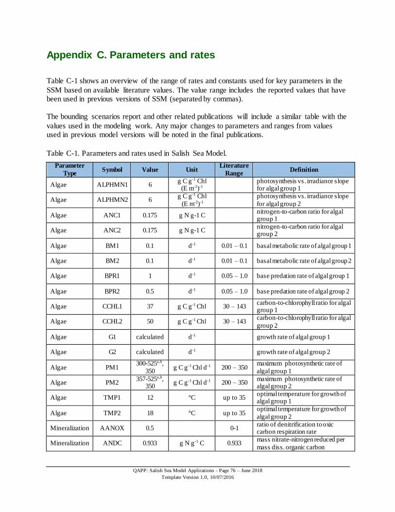
QAPP: Salish Sea Model Applications - Page 76 – June 2018
Template Version 1.0, 10/07/2016
Appendix C. Parameters and rates
Table C-1 shows an overview of the range of rates and constants used for key parameters in the
SSM based on available literature values. The value range includes the reported values that have been used in previous versions of SSM (separated by commas). The bounding scenarios report and other related publications will include a similar table with the
values used in the modeling work. Any major changes to parameters and ranges from values used in previous model versions will be noted in the final publications.
Table C-1. Parameters and rates used in Salish Sea Model.
Parameter
Type Symbol Value Unit
Literature
Range Definition
Algae ALPHMN1 6 g C g-1 Chl
(E m-2)-1
photosynthesis vs. irradiance slope for algal group 1
Algae ALPHMN2 6 g C g-1 Chl
(E m-2)-1
photosynthesis vs. irradiance slope
for algal group 2
Algae ANC1 0.175 g N g-1 C nitrogen-to-carbon ratio for algal group 1
Algae ANC2 0.175 g N g-1 C nitrogen-to-carbon ratio for algal group 2
Algae BM1 0.1 d-1 0.01 – 0.1 basal metabolic rate of algal group 1
Algae BM2 0.1 d-1 0.01 – 0.1 basal metabolic rate of algal group 2
Algae BPR1 1 d-1 0.05 – 1.0 base predation rate of algal group 1
Algae BPR2 0.5 d-1 0.05 – 1.0 base predation rate of algal group 2
Algae CCHL1 37 g C g-1 Chl 30 – 143 carbon-to-chlorophyll ratio for algal group 1
Algae CCHL2 50 g C g-1 Chl 30 – 143 carbon-to-chlorophyll ratio for algal
group 2
Algae G1 calculated d-1 growth rate of algal group 1
Algae G2 calculated d-1 growth rate of algal group 2
Algae PM1 300-525a,b,
350 g C g-1 Chl d-1 200 – 350
maximum photosynthetic rate of
algal group 1
Algae PM2 357-525a,b,
350 g C g-1 Chl d-1 200 – 350
maximum photosynthetic rate of algal group 2
Algae TMP1 12 °C up to 35 optimal temperature for growth of algal group 1
Algae TMP2 18 °C up to 35 optimal temperature for growth of
algal group 2
Mineralization AANOX 0.5 0-1 ratio of denitrification to oxic carbon respiration rate
Mineralization ANDC 0.933 g N g-1 C 0.933 mass nitrate-nitrogen reduced per
mass diss. organic carbon

QAPP: Salish Sea Model Applications - Page 77 – June 2018
Template Version 1.0, 10/07/2016
Parameter Type
Symbol Value Unit Literature
Range Definition
Mineralization AOCR 2.37,2.67 g O2 g-1C
oxygen-to-carbon mass ratio in production and respiration
Mineralization AONT 4.33 g O2 g-1 N
oxygen consumed per mass
ammonium nitrified
Mineralization DENIT calculated d-1 denitrification rate
Mineralization KHNDN 0.1 g N m-3 half-saturation conc. of nitrate required for denitrification
Mineralization KHNNT 0.5 g N m-3 half-saturation conc. of NH4
required for nitrification
Mineralization KHODOC 0.5 g O2 m-3
half-saturation conc. of DO required for oxic respiration
Mineralization KHONT 3 g O2 m-3
half-saturation conc. of DO required
for nitrification
Mineralization Kr calculated reaeration coefficient, calculated as a function of wind speed
Mineralization KTNT1 0.0045 °C-2 effect of sub-optimal temperature on nitrification
Mineralization KTNT2 0.0045 °C-2 effect of super-optimal temperature
on nitrification
Mineralization NTm 0.4 g N m-3 d-1 0.01 – 0.7 maximum nitrification rate
Mineralization TMNT 30 °C 25 – 35 optimal temperature for nitrification
Settling SS 0.25 m d-1 fixed solids settling rate
Settling WS1 0.6,0.4 m d-1 0 – 30 settling velocity of algal group 1
Settling WS2 0.3,0.2 m d-1 0 – 30 settling velocity of algal group 2
Settling WSLAB 10,5 m d-1 labile particulate organic solids settling rate
Settling WSREF 10,5 m d-1 refractory particulate organic matter settling rate
a Value specified in subbasins – Hood Canal, Whidbey Basin, Bellingham Bay, and South Puget Sound. b Value specified in selected shallow regions of Puget Sound known for low values of near-bed DO.

QAPP: Salish Sea Model Applications - Page 78 – June 2018
Template Version 1.0, 10/07/2016
Appendix D. Model equations
This section presents the equations from the model code that are currently being used in the
Salish Sea Model (SSM). These are equations based on CE-QUAL-ICM. More information about the processes and kinetics are documented in the user manual for CE-QUAL-ICM (1994). Some of these equations have been adapted to better represent conditions in the Salish Sea. For equations used specific for the Sediment Diagenesis and Ocean Acidification Modules, see their
respective reports (Pelletier et al., 2017a,b).
Phytoplankton (𝑔𝐶/𝑚3)
Two algae species are modeled. They are algal groups 1 and 2 (𝐵1 and 𝐵2 ). The equation for algal
group 1 is given here: 𝑑𝐵1
𝑑𝑡= 𝑁𝑃𝐵1 − 𝑃𝑅1 − 𝐵1𝑆𝑍− 𝐵1𝐿𝑍 − 𝑊𝑆𝐵1 × 𝑑𝐵1/𝑑𝑧
where 𝑁𝑃𝐵1 is net primary production: 𝑁𝑃𝐵1 = (𝑃1𝑀𝑖𝑛(𝑁𝐿1 ,𝑃𝐿1) × (1 − 𝛾1)/𝛼𝐶𝐶𝐻𝐿1 − 𝐵𝑀1) × 𝐵1 ,
where 𝑃1 is algal group 1 total growth: 𝑃1 = 𝑃𝑀1 × 𝑓𝑃𝑀(𝑇) × 𝐹𝐼1. 𝑃𝑀1 is maximum
photosynthesis rate (𝑔𝐶/𝑔𝐶𝐻𝐿/𝑑𝑎𝑦), 𝑓𝑃𝑀(𝑇) is temperature control on growth rate (0-
1), and 𝐹𝐼1 is light limitation (0-1). 𝑁𝐿1 is nitrogen limitation (Nitrate and Ammonia)
(0-1), 𝑃𝐿1 is phosphorus limitation (0-1), 𝛾1 is fraction of photosynthesis that is lost due to photochemical respiration (0-1), 𝛼𝐶𝐶𝐻𝐿1 is carbon to chlorophyll ratio (𝑔𝐶/𝑔𝐶𝐻𝐿),
𝐵𝑀1 is rate of loss due to basal metabolism (1/day).
𝑃𝑅1 is loss due to predation (𝑔𝐶/𝑚3/𝑑𝑎𝑦). 𝐵1𝑆𝑍 and 𝐵1𝐿𝑍 are micro and macro-zooplankton
consumption of algal group 1. 𝑊𝑆𝐵1 is settling speed (𝑚/𝑑𝑎𝑦).
Equation for algal group 2 𝐵2 is similar and omitted here.
Nitrate (𝒈𝑵/𝒎𝟑)
𝑑𝑁𝑂3
𝑑𝑡= 𝑁𝑇 − 𝛼𝑁𝐶 × 𝐷𝑁 − 𝑁𝑂3𝐴1 − 𝑁𝑂3𝐴2
where NT is gain of nitrate (𝑔𝑁/𝑚3/𝑑𝑎𝑦) due to nitrification, 𝛼𝑁𝐶 is stoichiometric ratio of
NO3 to LDOC in denitrification (𝑔𝑁/𝑔𝐶), and DN (𝑔𝐶/𝑚3/𝑑𝑎𝑦) is loss of labile dissolved
organic carbon (LDOC) due to denitrification:
𝐷𝑁 = 𝐾𝐿𝐷𝑂𝐶 × 𝑓𝑇𝑀𝑁𝐿 × 𝛼𝐴𝑁𝑂𝑋 × [𝐾𝐻𝑂,𝐷𝑂𝐶
𝐾𝐻𝑂,𝐷𝑂𝐶 +𝑂2] × [
𝑁𝑂3
𝐾𝐻𝑁𝐷𝑁 +𝑁𝑂3] × 𝐿𝐷𝑂𝐶
where 𝐾𝐿𝐷𝑂𝐶 is LDOC respiration rate (1/day). 𝛼𝐴𝑁𝑂𝑋 is ratio of denitrification to oxic carbon respiration rate (0-1), 𝐾𝐻𝑂,𝐷𝑂𝐶 is half-saturation concentration of dissolved
oxygen required for oxic respiration (𝑔𝑂2/𝑚3 ). 𝐾𝐻𝑁𝐷𝑁 is half-saturation concentration
of nitrate for denitrification (𝑔𝑁/𝑚3 ). LDOC is concentration of labile dissolved
organic matter (𝑔𝐶/𝑚3). 𝑓𝑇𝑀𝑁𝐿 = 𝑒(𝐾𝑇𝑀𝑁𝐿 (𝑇− 𝑇𝑅𝑀𝑁𝐿 )), where 𝐾𝑇𝑀𝑁𝐿 is the effect of
temperature deviations from 𝑇𝑅𝑀𝑁𝐿 on remineralization, T is temperature, and 𝑇𝑅𝑀𝑁𝐿 is the reference temperature for remineralization.
𝑁𝑂3𝐴1 is uptake of NO3 by algal group 1 (𝑔𝑁/𝑚3/𝑑𝑎𝑦) , 𝑁𝑂3𝐴2 is uptake of NO3 by algal
group 2 (𝑔𝑁/𝑚3/𝑑𝑎𝑦) .

QAPP: Salish Sea Model Applications - Page 79 – June 2018
Template Version 1.0, 10/07/2016
Ammonia (𝒈𝑵/𝒎𝟑)
𝑑𝑁𝐻4
𝑑𝑡= 𝑁𝐻4𝐴1 + 𝑁𝐻4𝐴2 + 𝑀𝑁𝐿𝐿𝐷𝑂𝑁 + 𝑀𝑁𝐿𝑅𝐷𝑂𝑁 − 𝑁𝑇 + 𝑁𝐻4𝑆𝑍 + 𝑁𝐻4𝐿𝑍
Where 𝑁𝐻4𝐴1 is production of NH4 due to basal metabolism and photochemical respiration, predation and uptake of NH4 by algal group 1 (𝑔𝑁/𝑚3/𝑑𝑎𝑦), and 𝑁𝐻4𝐴2 is production of NH4
due to basal metabolism and photochemical respiration, predation and uptake of NH4 by algal
group 2 (𝑔𝑁/𝑚3/𝑑𝑎𝑦). 𝑀𝑁𝐿𝐿𝐷𝑂𝑁 and 𝑀𝑁𝐿𝑅𝐷𝑂𝑁 are mineralization of LDON and RDON
respectively (𝑔𝑁/𝑚3/𝑑𝑎𝑦):
𝑀𝑁𝐿𝐿𝐷𝑂𝑁 =𝐷𝑂+𝐴𝐴𝑁𝑂𝑋 ×𝐾𝐻𝑂,𝐷𝑂𝐶
𝐾𝐻𝑂𝐷𝑂𝐶 +𝐷𝑂× 𝐾𝐿𝐷𝑂𝑁 × 𝑓𝑇𝑀𝑁𝐿 × 𝐿𝐷𝑂𝑁
𝑀𝑁𝐿𝑅𝐷𝑂𝑁 =𝐷𝑂+𝐴𝐴𝑁𝑂𝑋 ×𝐾𝐻𝑂,𝐷𝑂𝐶
𝐾𝐻𝑂𝐷𝑂𝐶 +𝐷𝑂 × 𝐾𝑅𝐷𝑂𝑁 × 𝑓𝑇𝑀𝑁𝐿 × 𝑅𝐷𝑂𝑁
where AANOX is the ratio of denitrification to oxic carbon respiration, 𝐾𝐿𝐷𝑂𝑁 and 𝐾𝑅𝐷𝑂𝑁 are mineralization rates of LDON and RDON respectively (1/day).
𝑁𝐻4𝑆𝑍 and 𝑁𝐻4𝐿𝑍 are recycled NH4 from the death of zooplankton (large and small species).
LDON (𝒈𝑵/𝒎𝟑)
𝑑𝐿𝐷𝑂𝑁
𝑑𝑡= 𝑓𝑁𝐿𝐷1 × 𝑁𝑃1 + 𝑓𝑁𝐿𝐷𝑃 × 𝑃𝑅1 × 𝛼𝑁𝐶1 + 𝑓𝑁𝐿𝐷2 × 𝑁𝑃2 + 𝑓𝑁𝐿𝐷𝑃 × 𝑃𝑅2 × 𝛼𝑁𝐶2
−𝑀𝑁𝐿𝐿𝐷𝑂𝑁 + 𝐾𝐻𝐷,𝐿𝑃𝑂𝑁 × 𝐿𝑃𝑂𝑁 + 𝐾𝐻𝐷,𝑅𝑃𝑂𝑁 × 𝑅𝑃𝑂𝑁 + 𝐿𝐷𝑂𝑁𝑆𝑍 + 𝐿𝐷𝑂𝑁𝐿𝑍
where 𝑓𝑁𝐿𝐷1 and 𝑓𝑁𝐿𝐷2 are the fraction of algal groups 1 and 2 metabolism released as LDON.
𝑁𝑃1 = 𝛼𝑁𝐶1 × 𝐶𝑃1 and 𝑁𝑃2 = 𝛼𝑁𝐶2 × 𝐶𝑃2 are photochemical respiration and basal metabolism
loss of first and second algae. 𝐶𝑃1 and 𝐶𝑃2 are loss of carbon due to photochemical respiration and basal metabolism of algal groups 1 and 2 (𝑔𝐶/𝑚3/𝑑𝑎𝑦):
𝐶𝑃1 = (𝑃1 × 𝛾1 + 𝐵𝑀1) × 𝐵1
𝐶𝑃2 = (𝑃2 × 𝛾2 + 𝐵𝑀2) × 𝐵2 where 𝑃1 and 𝑃2 are primary production rate (1/day) of first and second algae with light and nutrient limitation accounted for (1/day).
𝑓𝑁𝐿𝐷𝑃 is the fraction of algal predation released as LDON. 𝛼𝑁𝐶1 and 𝛼𝑁𝐶2 are nitrogen to carbon
ratios of first and second algae respectively (𝑔𝐶/𝑔𝑁). 𝐾𝐻𝐷,𝐿𝑃𝑂𝑁 is first order hydrolysis rate of
LPON (1/day) and 𝐾𝐻𝐷,𝑅𝑃𝑂𝑁 is first order hydrolysis rate of RPON (1/day).
RDON (𝒈𝑵/𝒎𝟑)
𝑑𝑅𝐷𝑂𝑁
𝑑𝑡= 𝑓𝑁𝑅𝐷1 × 𝑁𝑃1 + 𝑓𝑁𝑅𝐷𝑃 × 𝑃𝑅1 × 𝛼𝑁𝐶1 + 𝑓𝑁𝑅𝐷2 × 𝑁𝑃2 + 𝑓𝑁𝑅𝐷𝑃 × 𝑃𝑅2 × 𝛼𝑁𝐶2
−𝑀𝑁𝐿𝑅𝐷𝑂𝑁 + 𝑅𝐷𝑂𝑁𝑆𝑍 + 𝑅𝐷𝑂𝑁𝐿𝑍 − 𝐶𝐺𝑁 where 𝑓𝑁𝑅𝐷1 and 𝑓𝑁𝑅𝐷2 are the fraction of algal groups 1 and 2 metabolism released as RDON.
𝑓𝑁𝑅𝐷𝑃 is the fraction of algal predation released as RDON. 𝐶𝐺𝑁 is coagulation loss of RDON
(𝑔𝑁/𝑚3/𝑑𝑎𝑦):
𝐶𝐺𝑁 = 𝑆 × 𝐾𝑅𝐶𝑂𝐴𝐺 × 𝑅𝐷𝑂𝑁
where S is the influence of salinity on coagulation and 𝐾𝑅𝐶𝑂𝐴𝐺 is first order coagulation rate (1/day).
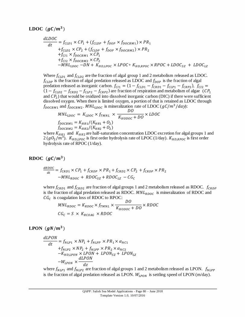
QAPP: Salish Sea Model Applications - Page 80 – June 2018
Template Version 1.0, 10/07/2016
LDOC (𝒈𝑪/𝒎𝟑)
𝑑𝐿𝐷𝑂𝐶
𝑑𝑡= 𝑓𝐶𝐿𝐷1 × 𝐶𝑃1 + (𝑓𝐶𝐿𝐷𝑃 + 𝑓𝐷𝑂𝑃 × 𝑓𝐷𝑂𝐶𝐵𝑀1) × 𝑃𝑅1
+𝑓𝐶𝐿𝐷2 × 𝐶𝑃2 + (𝑓𝐶𝐿𝐷𝑃 + 𝑓𝐷𝑂𝑃 × 𝑓𝐷𝑂𝐶𝐵𝑀2) × 𝑃𝑅2
+𝑓𝐶𝐼1 × 𝑓𝐷𝑂𝐶𝐵𝑀1 × 𝐶𝑃1
+𝑓𝐶𝐼2 × 𝑓𝐷𝑂𝐶𝐵𝑀2 × 𝐶𝑃2 −𝑀𝑁𝐿𝐿𝐷𝑂𝐶 −𝐷𝑁 + 𝐾𝐻𝐷,𝐿𝑃𝑂𝐶 × 𝐿𝑃𝑂𝐶+ 𝐾𝐻𝐷,𝑅𝑃𝑂𝐶 × 𝑅𝑃𝑂𝐶 + 𝐿𝐷𝑂𝐶𝑆𝑍 + 𝐿𝐷𝑂𝐶𝐿𝑍
Where 𝑓𝐶𝐿𝐷1 and 𝑓𝐶𝐿𝐷2 are the fraction of algal group 1 and 2 metabolism released as LDOC.
𝑓𝐶𝐿𝐷𝑃 is the fraction of algal predation released as LDOC and 𝑓𝐷𝑂𝑃 is the fraction of algal
predation released as inorganic carbon. 𝑓𝐶𝐼1 = (1 − 𝑓𝐶𝐿𝐷1 − 𝑓𝐶𝑅𝐷1 − 𝑓𝐶𝐿𝑃1 − 𝑓𝐶𝑅𝑃2), 𝑓𝐶𝐼2 =(1 − 𝑓𝐶𝐿𝐷2 − 𝑓𝐶𝑅𝐷2 − 𝑓𝐶𝐿𝑃2 − 𝑓𝐶𝑅𝑃2) are fraction of respiration and metabolism of algae (𝐶𝑃1
and 𝐶𝑃2) that would be oxidized into dissolved inorganic carbon (DIC) if there were sufficient dissolved oxygen. When there is limited oxygen, a portion of that is retained as LDOC through
𝑓𝐷𝑂𝐶𝐵𝑀1 and 𝑓𝐷𝑂𝐶𝐵𝑀2 . 𝑀𝑁𝐿𝐿𝐷𝑂𝐶 is mineralization rate of LDOC (𝑔𝐶/𝑚3/𝑑𝑎𝑦):
𝑀𝑁𝐿𝐿𝐷𝑂𝐶 = 𝐾𝐿𝐷𝑂𝐶 × 𝑓𝑇𝑀𝑁𝐿 × 𝐷𝑂
𝐾𝐻𝑂𝐷𝑂𝐶 + 𝐷𝑂× 𝐿𝐷𝑂𝐶
𝑓𝐷𝑂𝐶𝐵𝑀1 = 𝐾𝐻𝑅1/(𝐾𝐻𝑅1 + 𝑂2) 𝑓𝐷𝑂𝐶𝐵𝑀2 = 𝐾𝐻𝑅2/(𝐾𝐻𝑅2 + 𝑂2)
where 𝐾𝐻𝑅1 and 𝐾𝐻𝑅2 are half-saturation concentration LDOC excretion for algal groups 1 and 2 (𝑔𝑂2/𝑚3). 𝐾𝐻𝐷,𝐿𝑃𝑂𝐶 is first order hydrolysis rate of LPOC (1/day). 𝐾𝐻𝐷,𝑅𝑃𝑂𝐶 is first order
hydrolysis rate of RPOC (1/day).
RDOC (𝒈𝑪/𝒎𝟑)
𝑑𝑅𝐷𝑂𝐶
𝑑𝑡= 𝑓𝐶𝑅𝐷1 × 𝐶𝑃1 + 𝑓𝐶𝑅𝐷𝑃 × 𝑃𝑅1 + 𝑓𝐶𝑅𝐷2 × 𝐶𝑃2 + 𝑓𝐶𝑅𝐷𝑃 × 𝑃𝑅2
−𝑀𝑁𝐿𝑅𝐷𝑂𝐶 + 𝑅𝐷𝑂𝐶𝑆𝑍 + 𝑅𝐷𝑂𝐶𝐿𝑍 − 𝐶𝐺𝐶
where 𝑓𝐶𝑅𝐷1 and 𝑓𝐶𝑅𝐷2 are fraction of algal groups 1 and 2 metabolism released as RDOC. 𝑓𝐶𝑅𝐷𝑃
is the fraction of algal predation released as RDOC. 𝑀𝑁𝐿𝑅𝐷𝑂𝐶 is mineralization of RDOC and
𝐶𝐺𝐶 is coagulation loss of RDOC to RPOC:
𝑀𝑁𝐿𝑅𝐷𝑂𝐶 = 𝐾𝑅𝐷𝑂𝐶 × 𝑓𝑇𝑀𝑁𝐿 ×𝐷𝑂
𝐾𝐻𝑂𝐷𝑂𝐶 + 𝐷𝑂× 𝑅𝐷𝑂𝐶
𝐶𝐺𝐶 = 𝑆 × 𝐾𝑅𝐶𝑂𝐴𝐺 × 𝑅𝐷𝑂𝐶
LPON (𝒈𝑵/𝒎𝟑)
𝑑𝐿𝑃𝑂𝑁
𝑑𝑡= 𝑓𝑁𝐿𝑃1 × 𝑁𝑃1 + 𝑓𝑁𝐿𝑃𝑃 × 𝑃𝑅1 × 𝛼𝑁𝐶1
+𝑓𝑁𝐿𝑃2 × 𝑁𝑃2 + 𝑓𝑁𝐿𝑃𝑃 × 𝑃𝑅2 × 𝛼𝑁𝐶2
−𝐾𝐻𝐷,𝐿𝑃𝑂𝑁 × 𝐿𝑃𝑂𝑁 + 𝐿𝑃𝑂𝑁𝑆𝑍 + 𝐿𝑃𝑂𝑁𝐿𝑍
−𝑊𝐿𝑃𝑂𝑁 ×𝑑𝐿𝑃𝑂𝑁
𝑑𝑧
where 𝑓𝑁𝐿𝑃1 and 𝑓𝑁𝐿𝑃2 are fraction of algal groups 1 and 2 metabolism released as LPON. 𝑓𝑁𝐿𝑃𝑃
is the fraction of algal predation released as LPON. 𝑊𝐿𝑃𝑂𝑁 is settling speed of LPON (m/day).

QAPP: Salish Sea Model Applications - Page 81 – June 2018
Template Version 1.0, 10/07/2016
RPON (𝒈𝑵/𝒎𝟑)
𝑑𝑅𝑃𝑂𝑁
𝑑𝑡= 𝑓𝑁𝑅𝑃1 × 𝑁𝑃1 + 𝑓𝑁𝑅𝑃𝑃 × 𝑃𝑅1 × 𝛼𝑁𝐶1
+𝑓𝑁𝑅𝑃2 × 𝑁𝑃2 + 𝐹𝑁𝑅𝑃𝑃 × 𝑃𝑅2 × 𝛼𝑁𝐶2
−𝐾𝐻𝐷,𝑅𝑃𝑂𝑁 × 𝑅𝑃𝑂𝑁 + 𝑅𝑃𝑂𝑁𝑆𝑍 + 𝑅𝑃𝑂𝑁𝐿𝑍
+𝐶𝐺𝑁 − 𝑊𝑅𝑃𝑂𝑁 ×𝑅𝑃𝑂𝑁
𝑑𝑧
where 𝑓𝑁𝑅𝑃1 and 𝑓𝑁𝑅𝑃2 are fraction of algal groups 1 and 2 metabolism released as RPON. 𝑓𝑁𝑅𝑃𝑃
is the fraction of algal predation released as RPON. 𝑊𝑅𝑃𝑂𝑁 is settling speed of RPON (m/day).
LPOC (𝒈𝑪/𝒎𝟑)
𝑑𝐿𝑃𝑂𝐶
𝑑𝑡= 𝑓𝐶𝐿𝑃1 × 𝐶𝑃1 + 𝑓𝐶𝐿𝑃𝑃 × 𝑃𝑅1
+𝑓𝐶𝐿𝑃2 × 𝐶𝑃2 + 𝑓𝐶𝐿𝑃𝑃 × 𝑃𝑅2
−𝐾𝐻𝐷,𝐿𝑃𝑂𝐶 × 𝐿𝑃𝑂𝐶 + 𝐿𝑃𝑂𝐶𝑆𝑍 + 𝐿𝑃𝑂𝐶𝐿𝑍
−𝑊𝐿𝑃𝑂𝐶 ×𝑑𝐿𝑃𝑂𝐶
𝑑𝑧
where 𝑓𝐶𝐿𝑃1 and 𝑓𝐶𝐿𝑃2 are fraction of algal groups 1 and 2 metabolism released as LPOC. 𝑓𝐶𝐿𝑃𝑃
is the fraction of algal predation released as LPOC. 𝑊𝐿𝑃𝑂𝐶 is settling speed of LPOC (m/day).
RPOC (𝒈𝑪/𝒎𝟑)
𝑑𝑅𝑃𝑂𝐶
𝑑𝑡= 𝑓𝐶𝑅𝑃1 × 𝐶𝑃1 + 𝐹𝐶𝑅𝑃𝑃 × 𝑃𝑅1
+𝑓𝐶𝑅𝑃2 × 𝐶𝑃2 + 𝐹𝐶𝑅𝑃𝑃 × 𝑃𝑅2
−𝐾𝐻𝐷,𝑅𝑃𝑂𝐶 × 𝑅𝑃𝑂𝐶 + 𝑅𝑃𝑂𝐶𝑆𝑍 + 𝑅𝑃𝑂𝐶𝐿𝑍
+𝐶𝐺𝐶
−𝑊𝑅𝑃𝑂𝐶 ×𝑑𝑅𝑃𝑂𝐶
𝑑𝑧
where 𝑓𝐶𝑅𝑃1 and 𝑓𝐶𝑅𝑃2 are fraction of algal groups 1 and 2 metabolism released as LPOC. 𝑓𝐶𝑅𝑃𝑃
is the fraction of algal predation released as LPOC. 𝑊𝑅𝑃𝑂𝐶 is settling speed of RPOC (m/day).

QAPP: Salish Sea Model Applications - Page 82 – June 2018
Template Version 1.0, 10/07/2016
Oxygen (𝒈𝑶𝟐 /𝒎𝟑)
𝑑𝑂2
𝑑𝑡= 𝐷𝑂𝑅1 + 𝐷𝑂𝑅2 − 𝐷𝑂𝑃1 − 𝐷𝑂𝑃2 − 𝐷𝑂𝐷𝑂𝐶 − 𝑁𝑇 − 𝐷𝑂𝑆𝑍 − 𝐷𝑂𝐿𝑍
+𝐾𝑅𝐷𝑂 /𝑑𝑧𝑠 × (𝐷𝑂𝑆𝑎𝑡 − 𝑂2) − 𝑆𝑂𝐷/𝑑𝑧𝑏)
where 𝐷𝑂𝑅1 and 𝐷𝑂𝑅2 are the sum of production of oxygen due to photosynthesis, consumption of oxygen due to photochemical respiration and metabolism of algal groups 1 and 2
(𝑔𝑂2/𝑚3/𝑑𝑎𝑦):
𝐷𝑂𝑅1 = ((1.3 − 0.3𝑃𝑁1) × 𝑃1 − 𝑓𝑅𝐷𝑂1 × 𝐶𝑃1) × 𝛼𝑂𝐶,𝑅 × 𝐵1
𝐷𝑂𝑅2 = ((1.3 − 0.3𝑃𝑁2)× 𝑃2 − 𝑓𝑅𝐷𝑂2 × 𝐶𝑃2) × 𝛼𝑂𝐶,𝑅 × 𝐵2
where 𝑃𝑁1 and 𝑃𝑁2 are ammonia preference for nitrogen uptake by first and second algae respectively (0 ~1). 𝛼𝑂𝐶,𝑅 is oxygen to carbon stoichiometric ratio (𝑔𝑂2/𝑔𝐶)
𝑓𝑅𝐷𝑂1 = (1 − 𝑓𝐶𝐿𝐷1 − 𝑓𝐶𝑅𝐷1 − 𝑓𝐶𝐿𝑃1 − 𝑓𝐶𝑅𝑃1) ×𝑂2
𝐾𝐻𝑅1 + 𝑂2= 𝑓𝐶𝐼1 × (1 − 𝑓𝐷𝑂𝐶𝐵𝑀1)
𝑓𝑅𝐷𝑂2 = (1 − 𝑓𝐶𝐿𝐷2 − 𝑓𝐶𝑅𝐷2 − 𝑓𝐶𝐿𝑃2 − 𝑓𝐶𝑅𝑃2) ×𝑂2
𝐾𝐻𝑅2 + 𝑂2= 𝑓𝐶𝐼2 × (1 − 𝑓𝐷𝑂𝐶𝐵𝑀2)
𝐷𝑂𝑃1 and 𝐷𝑂𝑃2 are loss of oxygen due to predation on algal groups 1 and 2 (𝑔𝑂2/𝑚3/𝑑𝑎𝑦).
𝐷𝑂𝐷𝑂𝐶 is oxygen consumption due to mineralization of LDOC and RDOC (𝑔𝑂2/𝑚3/𝑑𝑎𝑦).
𝐷𝑂𝑃1 = 𝑓𝐷𝑂𝑃 × 𝑃𝑅1 ×𝑂2
𝐾𝐻𝑅1 + 𝑂2× 𝛼𝑂𝐶,𝑅
𝐷𝑂𝑃2 = 𝑓𝐷𝑂𝑃 × 𝑃𝑅2 ×𝑂2
𝐾𝐻𝑅2 + 𝑂2× 𝛼𝑂𝐶,𝑅
𝐷𝑂𝐷𝑂𝐶 = (𝑀𝑁𝐿𝐿𝐷𝑂𝐶 + 𝑀𝑁𝐿𝑅𝐷𝑂𝐶) × 𝛼𝑂𝐶,𝑅
For the surface layer, 𝐾𝑅𝐷𝑂 is surface reaeration rate for dissolved oxygen (m/day) and 𝑑𝑧𝑠 is surface layer thickness (m). For bottom layer, SOD is sediment oxygen demand (𝑔𝑂2/𝑚3/𝑑𝑎𝑦) and 𝑑𝑧𝑏 is bottom layer thickness (m). SOD is calculated by sediment diagenesis module.

QAPP: Salish Sea Model Applications - Page 83 – June 2018
Template Version 1.0, 10/07/2016
Appendix E. Method of evaluation of predicted violations of the DO criteria
The dissolved oxygen (DO) criteria are expressed as the lowest 1-day minimum oxygen
concentration that occurs anywhere in a water body and is not applied as a water-column average. The water quality standards establish both an absolute numeric threshold criterion and a relative difference criterion when the natural DO level (referred to as ‘reference conditions’ for this modeling work) is below the numeric criterion (WAC 173-201A-210(1)(d)). The DO
concentration is interpreted as the diel minimum for each day, since the health of aquatic species is tied predominantly to the pattern of daily minimum oxygen concentrations. Compliance with the water quality standards for DO will be based on the following steps:
1. For each day of the model simulation, find the minimum DO in each cell layer for the loading scenario (e.g. current conditions) and the reference condition.
2. Calculate the difference in diel minimum DO for each day comparing the loading scenario minus the reference condition for each cell layer. Negative values for the difference indicate
that the loading scenario has depleted DO relative to the reference scenario.
3. If any layer in a cell has a DO difference of less than -0.2 mg/l, and during the same day, the
diel minimum DO in that cell layer for the reference condition is less than the numeric water quality standard plus 0.2, then count that day as one day that is added to the cumulative number of days of non-compliance with the water quality standard for that cell.
4. Repeat for all days, and calculate the cumulative number of days for the entire simulation
period.
The difference of 0.2 mg/L of DO is based on the anthropogenic allowance of the second part of the water quality standards criterion for DO.

QAPP: Salish Sea Model Applications - Page 84 – June 2018
Template Version 1.0, 10/07/2016
Appendix F. Glossaries, acronyms, and abbreviations
Glossary of general terms Acidification: Reduction in the pH of the ocean over an extended period of time, caused
primarily by the update of carbon dioxide from the atmosphere.
Ambient: Background or away from point sources of contamination. Surrounding environmental condition.
Anthropogenic: Human-caused.
Clean Water Act: A federal act passed in 1972 that contains provisions to restore and maintain the quality of the nation’s waters. Section 303(d) of the Clean Water Act establishes the TMDL program.
Designated uses: Those uses specified in Chapter 173-201A WAC (Water Quality Standards
for Surface Waters of the State of Washington) for each water body or segment, regardless of whether or not the uses are currently attained.
Dissolved oxygen (DO): A measure of the amount of oxygen dissolved in water.
Effluent: An outflowing of water from a natural body of water or from a human-made structure.
For example, the treated outflow from a wastewater treatment plant.
Eutrophic: Nutrient rich and high in productivity resulting from human activities such as fertilizer runoff and leaky septic systems.
Margin of safety: Required component of TMDLs that accounts for uncertainty about the
relationship between pollutant loads and quality of the receiving water body.
Marine point sources: Wastewater treatment plants and industrial facilities that discharge directly into marine waters.
Model performance : Measures of the ability of a model to reproduce characteristics in the
processes and parameters being simulated.
National Pollutant Discharge Elimination System (NPDES): National program for issuing, modifying, revoking and reissuing, terminating, monitoring, and enforcing permits, and imposing and enforcing pretreatment requirements under the Clean Water Act. The NPDES
program regulates discharges from wastewater treatment plants, large factories, and other facilities that use, process, and discharge water back into lakes, streams, rivers, bays, and oceans.
Nonpoint source: Pollution that enters any waters of the state from any dispersed land-based or water-based activities, including but not limited to atmospheric deposition, surface-water runoff
from agricultural lands, urban areas, or forest lands, subsurface or underground sources, or discharges from boats or marine vessels not otherwise regulated under the NPDES program.

QAPP: Salish Sea Model Applications - Page 85 – June 2018
Template Version 1.0, 10/07/2016
Generally, any unconfined and diffuse source of contamination. Legally, any source of water pollution that does not meet the legal definition of “point source” in section 502(14) of the Clean Water Act.
Nutrient: Substance such as carbon, nitrogen, and phosphorus used by organisms to live and grow. Too many nutrients in the water can promote algal blooms and rob the water of oxygen vital to aquatic organisms.
Parameter: A physical chemical or biological property whose values determine environmental
characteristics or behavior.
pH: A measure of the acidity or alkalinity of water. A low pH value (0 to 7) indicates that an acidic condition is present, while a high pH (7 to 14) indicates a basic or alkaline condition. A pH of 7 is considered to be neutral. Since the pH scale is logarithmic, a water sample with a pH
of 8 is ten times more basic than one with a pH of 7.
Point source: Source of pollution that discharges at a specific location from pipes, outfalls, and conveyance channels to a surface water. Examples of point source discharges include municipal wastewater treatment plants, municipal stormwater systems, industrial waste treatment facilities,
and construction sites where more than 5 acres of land have been cleared.
Pollution: Contamination or other alteration of the physical, chemical, or biological properties of any waters of the state. This includes change in temperature, taste, color, turbidity, or odor of the waters. It also includes discharge of any liquid, gaseous, solid, radioactive, or other
substance into any waters of the state. This definition assumes that these changes will, or are likely to, create a nuisance or render such waters harmful, detrimental, or injurious to (1) public health, safety, or welfare, or (2) domestic, commercial, industrial, agricultural, recreational, or other legitimate beneficial uses, or (3) livestock, wild animals, birds, fish, or
other aquatic life.
Salish Sea: Formal name recognized by the U.S. and Canada to describe the estuarine waters that include the Strait of Juan de Fuca, Strait of Georgia, Puget Sound and all adjoining waters.
Sediment: Soil and organic matter that is covered with water (for example, river or lake
bottom).
Stormwater: The portion of precipitation that does not naturally percolate into the ground or evaporate but instead runs off roads, pavement, and roofs during rainfall or snow melt. Stormwater can also come from hard or saturated grass surfaces such as lawns, pastures,
playfields, and from gravel roads and parking lots.
Streamflow: Discharge of water in a surface stream (river or creek).
Surface waters of the state: Lakes, rivers, ponds, streams, inland waters, salt waters, wetlands and all other surface waters and water courses within the jurisdiction of Washington State.
Thalweg: The deepest and fastest moving portion of a stream.

QAPP: Salish Sea Model Applications - Page 86 – June 2018
Template Version 1.0, 10/07/2016
Watershed: A drainage area or basin in which all land and water areas drain or flow toward a central collector such as a stream, river, or lake at a lower elevation.
303(d) list: Section 303(d) of the federal Clean Water Act, requiring Washington State to
periodically prepare a list of all surface waters in the state for which beneficial uses of the water – such as for drinking, recreation, aquatic habitat, and industrial use – are impaired by pollutants. These are water quality-limited estuaries, lakes, and streams that fall short of state surface water quality standards and are not expected to improve within the next two years.
Acronyms and Abbreviations
Ωar Aragonite saturation state BMP Best management practice BNR Biological nutrient removal CESM The Community Earth System Model
DIC Dissolved inorganic carbon DIN Dissolved inorganic nitrogen DO (see Glossary above) DOC Dissolved organic carbon
e.g. For example Ecology Washington State Department of Ecology EIM Environmental Information Management database EPA U.S. Environmental Protection Agency
et al. And others FVCOM Finite-Volume Community Ocean Model GIS Geographic Information System software i.e. In other words
ICM Integrated Compartment Model MEL Manchester Environmental Laboratory MQO Measurement quality objective NOAA National Oceanic and Atmospheric Administration
NPDES (See Glossary above) PNNL Pacific Northwest National Lab PSDOM Puget Sound Dissolved Oxygen Model PSNSRP Puget Sound Nutrient Reduction Project
QA Quality assurance QAPP Quality assurance project plan QC Quality control RMSE Root-mean square error
SSM Salish Sea Model SOP Standard operating procedures TMDL (See Glossary above) TOC Total organic carbon
TSS (See Glossary above) USGS United States Geological Survey UW University of Washington WAC Washington Administrative Code

QAPP: Salish Sea Model Applications - Page 87 – June 2018
Template Version 1.0, 10/07/2016
WRF Weather Research Forecasting WQS Water Quality Standards WWTP Wastewater treatment plant
Y Year Units of Measurement
°C degrees centigrade cfs cubic feet per second ft feet
g gram, a unit of mass kg kilograms, a unit of mass equal to 1,000 grams kg/d kilograms per day km kilometer, a unit of length equal to 1,000 meters
m meter m3/s cubic meters per second, a unit of flow mgd million gallons per day mg/L milligrams per liter
NTU nephelometric turbidity units psu practical salinity units s.u. standard units
Quality Assurance Glossary Accreditation: A certification process for laboratories, designed to evaluate and document a
lab’s ability to perform analytical methods and produce acceptable data. For Ecology, it is
“Formal recognition by (Ecology)…that an environmental laboratory is capable of producing accurate analytical data.” [WAC 173-50-040] (Kammin, 2010)
Accuracy: The degree to which a measured value agrees with the true value of the measured property. USEPA recommends that this term not be used, and that the terms precision and bias be used to convey the information associated with the term accuracy. (USGS, 1998)
Analyte: An element, ion, compound, or chemical moiety (pH, alkalinity) which is to be determined. The definition can be expanded to include organisms, e.g., fecal coliform, Klebsiella. (Kammin, 2010)
Bias: The difference between the population mean and the true value. Bias usually describes a systematic difference reproducible over time, and is characteristic of both the measurement system, and the analyte(s) being measured. Bias is a commonly used data quality indicator (DQI). (Kammin, 2010; Ecology, 2004)
Blank: A synthetic sample, free of the analyte(s) of interest. For example, in water analysis, pure water is used for the blank. In chemical analysis, a blank is used to estimate the analytical response to all factors other than the analyte in the sample. In general, blanks are used to assess

QAPP: Salish Sea Model Applications - Page 88 – June 2018
Template Version 1.0, 10/07/2016
possible contamination or inadvertent introduction of analyte during various stages of the sampling and analytical process. (USGS, 1998)
Calibration: The process of establishing the relationship between the response of a measurement system and the concentration of the parameter being measured. (Ecology, 2004)
Check standard: A substance or reference material obtained from a source independent from
the source of the calibration standard; used to assess bias for an analytical method. This is an obsolete term, and its use is highly discouraged. See Calibration Verification Standards, Lab Control Samples (LCS), Certified Reference Materials (CRM), and/or spiked blanks. These are all check standards, but should be referred to by their actual designator, e.g., CRM, LCS.
(Kammin, 2010; Ecology, 2004)
Comparability: The degree to which different methods, data sets and/or decisions agree or can be represented as similar; a data quality indicator. (USEPA, 1997)
Completeness: The amount of valid data obtained from a project compared to the planned amount. Usually expressed as a percentage. A data quality indicator. (USEPA, 1997)
Continuing Calibration Verification Standard (CCV): A QC sample analyzed with samples to check for acceptable bias in the measurement system. The CCV is usually a midpoint calibration standard that is re-run at an established frequency during the course of an analytical run. (Kammin, 2010)
Control chart: A graphical representation of quality control results demonstrating the performance of an aspect of a measurement system. (Kammin, 2010; Ecology 2004)
Control limits: Statistical warning and action limits calculated based on control charts. Warning limits are generally set at +/- 2 standard deviations from the mean, action limits at +/- 3 standard deviations from the mean. (Kammin, 2010)
Data integrity: A qualitative DQI that evaluates the extent to which a data set contains data that is misrepresented, falsified, or deliberately misleading. (Kammin, 2010)
Data Quality Indicators (DQI): Commonly used measures of acceptability for environmental
data. The principal DQIs are precision, bias, representativeness, comparability, completeness, sensitivity, and integrity. (USEPA, 2006)
Data Quality Objectives (DQO): Qualitative and quantitative statements derived from
systematic planning processes that clarify study objectives, define the appropriate type of data, and specify tolerable levels of potential decision errors that will be used as the basis for establishing the quality and quantity of data needed to support decisions. (USEPA, 2006)
Data set: A grouping of samples organized by date, time, analyte, etc. (Kammin, 2010)
QAPP: Salish Sea Model Applications - Page 89 – June 2018
Template Version 1.0, 10/07/2016
Data validation: An analyte-specific and sample-specific process that extends the evaluation of data beyond data verification to determine the usability of a specific data set. It involves a detailed examination of the data package, using both professional judgment, and objective
criteria, to determine whether the MQOs for precision, bias, and sensitivity have been met. It may also include an assessment of completeness, representativeness, comparability and integrity, as these criteria relate to the usability of the data set. Ecology considers four key criteria to determine if data validation has actually occurred. These are:
Use of raw or instrument data for evaluation.
Use of third-party assessors.
Data set is complex.
Use of EPA Functional Guidelines or equivalent for review. Examples of data types commonly validated would be:
Gas Chromatography (GC).
Gas Chromatography-Mass Spectrometry (GC-MS).
Inductively Coupled Plasma (ICP).
The end result of a formal validation process is a determination of usability that assigns qualifiers to indicate usability status for every measurement result. These qualifiers include:
No qualifier – data are usable for intended purposes.
J (or a J variant) – data are estimated, may be usable, may be biased high or low.
REJ – data are rejected, cannot be used for intended purposes. (Kammin, 2010; Ecology, 2004).
Data verification: Examination of a data set for errors or omissions, and assessment of the Data Quality Indicators related to that data set for compliance with acceptance criteria (MQOs). Verification is a detailed quality review of a data set. (Ecology, 2004)
Detection limit (limit of detection): The concentration or amount of an analyte which can be determined to a specified level of certainty to be greater than zero. (Ecology, 2004)
Duplicate samples: Two samples taken from and representative of the same population, and
carried through and steps of the sampling and analytical procedures in an identical manner. Duplicate samples are used to assess variability of all method activities including sampling and analysis. (USEPA, 1997)
Field blank: A blank used to obtain information on contamination introduced during sample collection, storage, and transport. (Ecology, 2004) Initial Calibration Verification Standard (ICV): A QC sample prepared independently of
calibration standards and analyzed along with the samples to check for acceptable bias in the measurement system. The ICV is analyzed prior to the analysis of any samples. (Kammin, 2010)
Laboratory Control Sample (LCS): A sample of known composition prepared using contaminant-free water or an inert solid that is spiked with analytes of interest at the midpoint of

QAPP: Salish Sea Model Applications - Page 90 – June 2018
Template Version 1.0, 10/07/2016
the calibration curve or at the level of concern. It is prepared and analyzed in the same batch of regular samples using the same sample preparation method, reagents, and analytical methods employed for regular samples. (USEPA, 1997)
Matrix spike: A QC sample prepared by adding a known amount of the target analyte(s) to an aliquot of a sample to check for bias due to interference or matrix effects. (Ecology, 2004)
Measurement Quality Objectives (MQOs): Performance or acceptance criteria for individual data quality indicators, usually including precision, bias, sensitivity, completeness, comparability, and representativeness. (USEPA, 2006)
Measurement result: A value obtained by performing the procedure described in a method. (Ecology, 2004)
Method: A formalized group of procedures and techniques for performing an activity (e.g.,
sampling, chemical analysis, data analysis), systematically presented in the order in which they are to be executed. (EPA, 1997)
Method blank: A blank prepared to represent the sample matrix, prepared and analyzed with a
batch of samples. A method blank will contain all reagents used in the preparation of a sample, and the same preparation process is used for the method blank and samples. (Ecology, 2004; Kammin, 2010)
Method Detection Limit (MDL): This definition for detection was first formally advanced in 40CFR 136, October 26, 1984 edition. MDL is defined there as the minimum concentration of an analyte that, in a given matrix and with a specific method, has a 99% probability of being identified, and reported to be greater than zero. (Federal Register, October 26, 1984)
Percent Relative Standard Deviation (%RSD): A statistic used to evaluate precision in environmental analysis. It is determined in the following manner:
%RSD = (100 * s)/x
where s is the sample standard deviation and x is the mean of results from more than two replicate samples. (Kammin, 2010)
Parameter: A specified characteristic of a population or sample. Also, an analyte or grouping
of analytes. Benzene and nitrate + nitrite are all “parameters.” (Kammin, 2010; Ecology, 2004) Population: The hypothetical set of all possible observations of the type being investigated. (Ecology, 2004)
Precision: The extent of random variability among replicate measurements of the same property; a data quality indicator. (USGS, 1998)
Quality assurance (QA): A set of activities designed to establish and document the reliability and usability of measurement data. (Kammin, 2010)
QAPP: Salish Sea Model Applications - Page 91 – June 2018
Template Version 1.0, 10/07/2016
Quality Assurance Project Plan (QAPP): A document that describes the objectives of a project, and the processes and activities necessary to develop data that will support those objectives. (Kammin, 2010; Ecology, 2004)
Quality control (QC): The routine application of measurement and statistical procedures to assess the accuracy of measurement data. (Ecology, 2004)
Relative Percent Difference (RPD): RPD is commonly used to evaluate precision. The following formula is used:
[Abs(a-b)/((a + b)/2)] * 100 where “Abs()” is absolute value and a and b are results for the two replicate samples. RPD can
be used only with 2 values. Percent Relative Standard Deviation is (%RSD) is used if there are results for more than 2 replicate samples (Ecology, 2004).
Replicate samples: Two or more samples taken from the environment at the same time and
place, using the same protocols. Replicates are used to estimate the random variability of the material sampled. (USGS, 1998)
Representativeness: The degree to which a sample reflects the population from which it is
taken; a data quality indicator. (USGS, 1998)
Sample (field): A portion of a population (environmental entity) that is measured and assumed to represent the entire population. (USGS, 1998)
Sample (statistical): A finite part or subset of a statistical population. (USEPA, 1997)
Sensitivity: In general, denotes the rate at which the analytical response (e.g., absorbance,
volume, meter reading) varies with the concentration of the parameter being determined. In a specialized sense, it has the same meaning as the detection limit. (Ecology, 2004) Spiked blank: A specified amount of reagent blank fortified with a known mass of the target
analyte(s); usually used to assess the recovery efficiency of the method. (USEPA, 1997)
Spiked sample: A sample prepared by adding a known mass of target analyte(s) to a specified amount of matrix sample for which an independent estimate of target analyte(s) concentration is
available. Spiked samples can be used to determine the effect of the matrix on a method’s recovery efficiency. (USEPA, 1997)
Split sample: A discrete sample subdivided into portions, usually duplicates (Kammin, 2010)
Standard Operating Procedure (SOP): A document which describes in detail a reproducible and repeatable organized activity. (Kammin, 2010)
Surrogate: For environmental chemistry, a surrogate is a substance with properties similar to those of the target analyte(s). Surrogates are unlikely to be native to environmental samples. They are added to environmental samples for quality control purposes, to track extraction

QAPP: Salish Sea Model Applications - Page 92 – June 2018
Template Version 1.0, 10/07/2016
efficiency and/or measure analyte recovery. Deuterated organic compounds are examples of surrogates commonly used in organic compound analysis. (Kammin, 2010)
Systematic planning: A step-wise process which develops a clear description of the goals and objectives of a project, and produces decisions on the type, quantity, and quality of data that will be needed to meet those goals and objectives. The DQO process is a specialized type of systematic planning. (USEPA, 2006)
References for QA Glossary
Ecology, 2004. Guidance for the Preparation of Quality Assurance Project Plans for Environmental Studies. https://fortress.wa.gov/ecy/publications/SummaryPages/0403030.html
Kammin, B., 2010. Definition developed or extensively edited by William Kammin, 2010. Washington State Department of Ecology, Olympia, WA.
USEPA, 1997. Glossary of Quality Assurance Terms and Related Acronyms. U.S. Environmental Protection Agency.
USEPA, 2006. Guidance on Systematic Planning Using the Data Quality Objectives Process EPA QA/G-4. U.S. Environmental Protection Agency. http://www.epa.gov/quality/qs-docs/g4-final.pdf
USGS, 1998. Principles and Practices for Quality Assurance and Quality Control. Open-File
Report 98-636. U.S. Geological Survey. http://ma.water.usgs.gov/fhwa/products/ofr98-636.pdf


![CONNECTING THE DOTS: Orcas, Salmon and Toxic Chemicals in the Salish Sea · 2019-12-16 · Administration [NOAA], 2015). Icons of the Salish Sea, which includes the marine waters](https://static.fdocuments.in/doc/165x107/5f44369df28c160257725d68/connecting-the-dots-orcas-salmon-and-toxic-chemicals-in-the-salish-sea-2019-12-16.jpg)