Qualitative behaviour of numerical methods for … behaviour of numerical methods for SDEs and...
46
Qualitative behaviour of numerical methods for SDEs and application to homogenization K. C. Zygalakis Oxford Centre For Collaborative Applied Mathematics, University of Oxford. Center for Nonlinear Analysis, Carnegie Mellon University, 20/10/2011 K. C. Zygalakis (University of Oxford) Modified Equations for SDEs 1 / 45
Transcript of Qualitative behaviour of numerical methods for … behaviour of numerical methods for SDEs and...

Qualitative behaviour of numerical methods for SDEsand application to homogenization
K. C. Zygalakis
Oxford Centre For Collaborative Applied Mathematics,University of Oxford.
Center for Nonlinear Analysis,Carnegie Mellon University,
20/10/2011
K. C. Zygalakis (University of Oxford) Modified Equations for SDEs 1 / 45

Outline
1 Modified Equations
ODE theory.Main idea for SDEs.Different numerical methods and Associated Modified Equations.Numerical examples.
2 Application to Homogenization
Long time behaviour and homogenization.Numerical algorithms/results.From homogenization to averaging in cellular flows.
3 Higher order numerical methods based on modified equations.
Key idea.One simple example.
K. C. Zygalakis (University of Oxford) Modified Equations for SDEs 2 / 45

Introduction
Motivating example
K. C. Zygalakis (University of Oxford) Modified Equations for SDEs 3 / 45

Introduction
Interesting Question
The two numerical methods have the same order of convergence butcompletely different qualitative behaviour.
Is there a way to distinguish between these two methods?
A very powerful tool for addressing this question is backward erroranalysis (modified equations).
K. C. Zygalakis (University of Oxford) Modified Equations for SDEs 4 / 45

Introduction Ordinary Differential Equations
Modified equations for ODEs
dx
dt= f (x),
and let xn be a numerical approximation of x of order p:
|x(nh)− xn| = O(hp).
Can I find X (t) satisfying another ODE (modified equation) such that:
|X (nh)− xn| = O(hp+q).
K. C. Zygalakis (University of Oxford) Modified Equations for SDEs 5 / 45
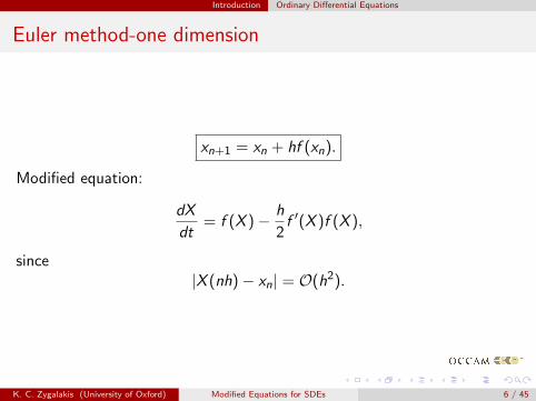
Introduction Ordinary Differential Equations
Euler method-one dimension
xn+1 = xn + hf (xn).
Modified equation:
dX
dt= f (X )− h
2f ′(X )f (X ),
since|X (nh)− xn| = O(h2).
K. C. Zygalakis (University of Oxford) Modified Equations for SDEs 6 / 45

Introduction Ordinary Differential Equations
Sketch proof
dX
dt= f (X ) + hg(X ).
X (h) = X (0) +
∫ h
0
(f (X (s)) + hg(X (s))) ds
= X (0) + hf (X (0)) + h2g(X (0)) +h2
2f (X (0))f ′(X (0)) +O(h3).
Assume x0 = X (0) then
X (h)− x1 = h2
(g(X (0)) +
1
2f (X (0))f ′(X (0))
)+O(h3),
and thus
g(x) = −1
2f (x)f ′(x).
K. C. Zygalakis (University of Oxford) Modified Equations for SDEs 7 / 45

Introduction Stochastic Differential Equations
Stochastic Differential Equations and Numerical Methods
dx = u(x)dt + σ(x)dWt ,
Euler method:xn+1 = xn + hu(xn) +
√hσ(xn)ξn,
θ-Milstein method:
xn+1 = xn +θhu(xn+1)+(1−θ)hu(xn)+√
hσ(xn)ξn +h
2σ(xn)σ(1)(xn)(ξ2
n−1),
where ξn ∼ N (0, 1).
K. C. Zygalakis (University of Oxford) Modified Equations for SDEs 8 / 45
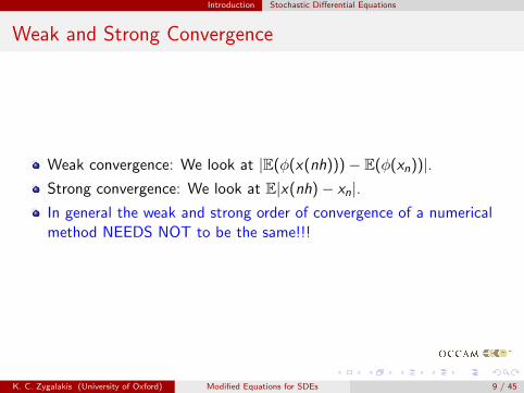
Introduction Stochastic Differential Equations
Weak and Strong Convergence
Weak convergence: We look at |E(φ(x(nh)))− E(φ(xn))|.Strong convergence: We look at E|x(nh)− xn|.In general the weak and strong order of convergence of a numericalmethod NEEDS NOT to be the same!!!
K. C. Zygalakis (University of Oxford) Modified Equations for SDEs 9 / 45

Introduction Stochastic Differential Equations
Statement of the Problem
Let x(t) satisfy the following SDE:
dx = u1(x)dt + σ1(x)dWt ,
and xn be its numerical approximation at T = nh by a weak p-ordermethod i.e
|E(φ(x(T )))− E(φ(xn))| = O(hp), ∀φ ∈ C∞.
We want to develop a procedure that allows us to evaluate the propertiesof our weak numerical scheme.
K. C. Zygalakis (University of Oxford) Modified Equations for SDEs 10 / 45

Introduction Stochastic Differential Equations
First Modified Equation
We want to find a modified SDE of the form (i.e., find v2 and σ2)
dx = [u1(x) + hu2(x)] + [σ1(x) + hσ2(x)] dWt ,
for which
|E(φ(x(T )))− E(φ(xn))| = O(hp+1), ∀φ ∈ C∞.
For the rest of the talk we concentrate in the case where p = 1.
K. C. Zygalakis (University of Oxford) Modified Equations for SDEs 11 / 45

Main Idea
Generators for ODEs and SDEs
ODE:
dx = h(x)dt,
Lu := h(x) · ∇xu.
SDE:
dx = h(x)dt + σ(x)dWt ,
Lu := h(x) · ∇xu +1
2σ(x)σT (x) : ∇x∇xu.
K. C. Zygalakis (University of Oxford) Modified Equations for SDEs 12 / 45
Main Idea
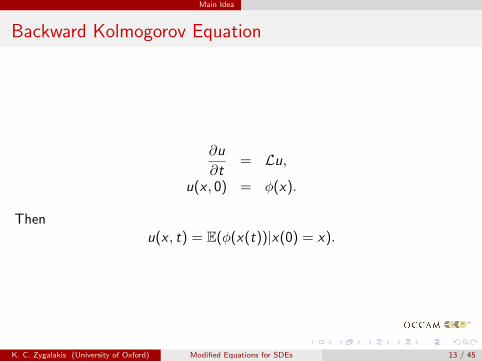
Backward Kolmogorov Equation
∂u
∂t= Lu,
u(x , 0) = φ(x).
Thenu(x , t) = E(φ(x(t))|x(0) = x).
K. C. Zygalakis (University of Oxford) Modified Equations for SDEs 13 / 45

Main Idea
Stochastic B-series
By integrating over time the backward Kolmogorov Equation and taking aTaylor expansion of u(x , s) around s = 0, we obtain, (assumingappropriate smoothness of the drift and diffusion term)
u(x , h)− φ(x) =∞∑k=0
hk+1
(k + 1)!Lk+1φ(x).
Note that in the case where φ(x) = x , σ(x) = 0, this expansioncorrespond to the B-series expansion of the ODE
dx = v1(x)dt.
K. C. Zygalakis (University of Oxford) Modified Equations for SDEs 14 / 45
Main Idea
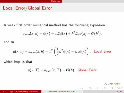
Local Error/Global Error
A weak first order numerical method has the following expansion
unum(x , h)− φ(x) = hLφ(x) + h2Leφ(x) +O(h3),
and so
u(x , h)− unum(x , h) = h2
(1
2L2φ(x)− Leφ(x)
), Local Error
which implies that
u(x ,T )− unum(x ,T ) = O(h). Global Error
K. C. Zygalakis (University of Oxford) Modified Equations for SDEs 15 / 45

Main Idea
Generator of the Modified Equation
Remember that the 1-st modified equation is of the form
dx = [u1(x) + hu2(x)] + [σ1(x) + hσ2(x)] dWt .
Its generator L can be written as
L = L0 + hL1 + h2L2,
where L0 is the generator of the original SDE and
L1φ := u2(x)dφ
dx+ σ1(x)σ2(x)
d2φ
dx2.
K. C. Zygalakis (University of Oxford) Modified Equations for SDEs 16 / 45

Main Idea
Main Equation
If we now subtract the Taylor expansion of the numerical method from thestochastic B-series of the modified equation we see that in order for thelocal error to be O(∆t3) we need
L1φ = Leφ−1
2L2
0φ, ∀φ ∈ C∞.
K. C. Zygalakis (University of Oxford) Modified Equations for SDEs 17 / 45

Different Numerical Methods
Euler-Maryama Method
In the case of Euler-Maryama method in the case of multiplicative noise itturns out that a modified equation does not exist since
L1φ 6= · · ·+σ3
1(x)
2σ
(1)1 (x)φ(3)(x).
as L1 is a second order partial differential operator!!!
K. C. Zygalakis (University of Oxford) Modified Equations for SDEs 18 / 45

Different Numerical Methods
θ-Milstein Method
u2(x) =
(θ − 1
2
)(v1(x)v
(1)1 (x) +
σ21(x)
2v
(2)1 (x)
),
σ2(x) =
(θ − 1
2
)σ1(x)v
(1)1 (x)− 1
2v1(x)σ
(1)1 (x)− σ2
1(x)
4σ
(2)1 (x).
K. C. Zygalakis (University of Oxford) Modified Equations for SDEs 19 / 45

Numerical examples SDEs Driven by Multiplicative Noise
Geometric Brownian motion
dx = µxdt + σxdWt ,
dX =
[(µ− h
2µ2
)X
]dt + σX (1− hµ) dWt .
10−3
10−2
10−1
10−5
10−4
10−3
10−2
10−1
100
∆ t
erro
r
original SDEmodified SDE
10−3
10−2
10−1
10−4
10−3
10−2
10−1
100
101
∆ t
erro
r
original SDEmodified SDE
First moment Second moment
K. C. Zygalakis (University of Oxford) Modified Equations for SDEs 20 / 45

Numerical examples ∞ Modified equations
Linear SDEs with additive noise
dx = Axdt + ΣdWt ,
Numerical Approximation:
x(h) = A(h)x + f (h, ω).
Example (Euler-Maryama):
A(h) = (I + hA),
f (h, ω) = Σ√
hξ.
K. C. Zygalakis (University of Oxford) Modified Equations for SDEs 21 / 45

Numerical examples ∞ Modified equations
∞ Modified Equation and its coefficients
dx = Axdt + ΣdWt ,
A =log(A(h))
h,
eAhΣΣT eATh − ΣΣT = AJ + JAT ,
whereJ = E(ff T ).
K. C. Zygalakis (University of Oxford) Modified Equations for SDEs 22 / 45

Numerical examples ∞ Modified equations
Orstein Uhlenbeck Process
dx = −γxdt + σdWt .
Forward Euler:
A =log(1− γh)
h,
Σ = σ
√2 log(1− γh)
(1− γh)2 − 1.
Backward Euler:
A = − log(1 + γh)
h,
Σ = σ
√2 log(1 + γh)
1− (1 + γh)−2.
K. C. Zygalakis (University of Oxford) Modified Equations for SDEs 23 / 45

Numerical examples ∞ Modified equations
Invariant Measure
limt→∞
E(x2(t)) =σ2
2γ − γ2h, Forward Euler
limt→∞
E(x2(t)) =σ2(1 + γh)
2γ + γ2h, Backward Euler.
0 0.05 0.1 0.15 0.2 0.25 0.3 0.35 0.4 0.45 0.50.48
0.5
0.52
0.54
0.56
0.58
0.6
0.62
0.64
0.66
0.68
∆ t
Var
(x)
numerical solution∞ modified equation
0 0.05 0.1 0.15 0.2 0.25 0.3 0.35 0.4 0.45 0.50.45
0.5
0.55
0.6
0.65
0.7
0.75
0.8
0.85
0.9
0.95
∆ t
Var
(x)
numerical solution∞ modified equation
Forward Euler Backward Euler
Figure: limt→∞ E(x2(t)) as a function of h.
K. C. Zygalakis (University of Oxford) Modified Equations for SDEs 24 / 45

An application to homogenization Long Time Behaviour and Homogenization
Passive Tracers, Effective Diffusivity
dx = v(x)dt + σdWt ,
where v(x) is a periodic function. It is possible to show usinghomogenization that
limt→∞
E(x(t)⊗ x(t))
2t= K.
We will refer to K as the effective diffusivity matrix
K. C. Zygalakis (University of Oxford) Modified Equations for SDEs 25 / 45

An application to homogenization Long Time Behaviour and Homogenization
Velocity Field of Interest
Example
We are interested in the following 2-dimensional incompressible velocityfield
v(x) = ∇⊥Ψ(x), where Ψ(x) = sin x1 sin x2
Result
In this case it is known that K = DI2, where D ∈ R depending on σ forpassive tracers and that the following result is true for passive tracers
D(σ) ∼ σ, σ � 1
K. C. Zygalakis (University of Oxford) Modified Equations for SDEs 26 / 45
An application to homogenization Long Time Behaviour and Homogenization
Key Property of the Velocity Field
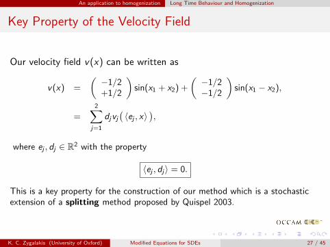
Our velocity field v(x) can be written as
v(x) =
(−1/2+1/2
)sin(x1 + x2) +
(−1/2−1/2
)sin(x1 − x2),
=2∑
j=1
djvj(〈ej , x〉
),
where ej , dj ∈ R2 with the property
〈ej , dj〉 = 0.
This is a key property for the construction of our method which is a stochasticextension of a splitting method proposed by Quispel 2003.
K. C. Zygalakis (University of Oxford) Modified Equations for SDEs 27 / 45

An application to homogenization Numerical algorithm/results
Description of the Method:
The method in the case of passive tracers involves these 3 steps:
Step 1: Solve x1 = d1v1
(〈e1, x1〉
),
Step 2: Solve x2 = d2v2
(〈e2, x2〉
),
Step 3: Solve x3 = σβ1.
K. C. Zygalakis (University of Oxford) Modified Equations for SDEs 28 / 45

An application to homogenization Numerical algorithm/results
The Deterministic Case
Splitting method for σ = 0. Euler method for σ = 0.
K. C. Zygalakis (University of Oxford) Modified Equations for SDEs 29 / 45

An application to homogenization Numerical algorithm/results
The Case σ � 1
Splitting method for σ = 10−2. Euler method for σ = 10−2.
K. C. Zygalakis (University of Oxford) Modified Equations for SDEs 30 / 45

An application to homogenization Numerical algorithm/results
Calculating Effective Diffusivities
10!2 10!1 100 10110!3
10!2
10!1
100
101
102
!
K
Volume preservingEuler!Maruyama
10!3 10!2 10!110!6
10!5
10!4
10!3
10!2
10!1
!
KComparison of the two methods. Splitting Method.
K. C. Zygalakis (University of Oxford) Modified Equations for SDEs 31 / 45

An application to homogenization Numerical algorithm/results
Mean Hamiltonian
We apply Ito ’s formula to H = Ψ we obtain
dΨ
dt= −σ2Ψ + M.T
which implies that the mean Hamiltonian decays like e−σ2t
K. C. Zygalakis (University of Oxford) Modified Equations for SDEs 32 / 45

An application to homogenization Numerical algorithm/results
Numerical calculation of the mean Hamiltonian with thetwo methods
0 1 2 3 4 5 6 7 8 9 10x 104
!0.1
0
0.1
0.2
0.3
0.4
0.5
0.6
0.7
0.8
t
Mea
n Ha
milt
onia
n
Euler MethodStochastic Splitting MethodTheory
Figure: Mean value of the Hamiltonian as a function of time, for∆t = 10−1, σ = 10−2.
K. C. Zygalakis (University of Oxford) Modified Equations for SDEs 33 / 45

An application to homogenization Numerical algorithm/results
Modified Equations for the Euler Method
dx =
(v(x)− ∆t
2(∇v(x))v(x)− σ2∆t
4∆v(x)
)dt
+ σ
(1− ∆t
2∇vT (x)
)dWt .
dΨ
dt= −∆t
2(cos2 x1 + cos2 x2)Ψ− σ2Ψ(1 + ∆t cos x1 cos x2)
+σ2∆2t
4(cos2 x1 cos2 x2Ψ−Ψ3) + M∆t .
K. C. Zygalakis (University of Oxford) Modified Equations for SDEs 34 / 45

An application to homogenization From Homogenization to averaging in cellular flows.
Statement of the problem
u(x) = ∇⊥Ψ(x), Ψ(x) =1
πsinπx1 sinπx2.
Xt satisfies the following SDE
dXt = −Au(Xt)dt +√
2dWt .
Exit time problem
−∆τ + Au · ∇τ = 1 in D,
τ = 0 on ∂D,
where D = [−L/2, L/2]× [−L/2, L/2].
K. C. Zygalakis (University of Oxford) Modified Equations for SDEs 35 / 45

An application to homogenization From Homogenization to averaging in cellular flows.
Known results and open questions
1 A fixed, L→∞, homogenization (τ →∞).
2 L fixed, A→∞, averaging (τ → 0).
3 If D = BL a disk of radius L, then τ(x) ∼ L2 − |x |2.4 A = Lα and L→∞
α < 4, homogenization (τ ∼ L2−α/2).α > 4, averaging (τ ∼ L2−α/2).
Question
How about α = 4?
K. C. Zygalakis (University of Oxford) Modified Equations for SDEs 36 / 45
An application to homogenization From Homogenization to averaging in cellular flows.
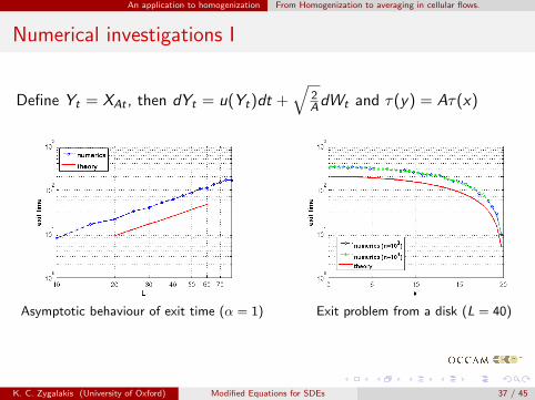
Numerical investigations I
Define Yt = XAt , then dYt = u(Yt)dt +√
2AdWt and τ(y) = Aτ(x)
Asymptotic behaviour of exit time (α = 1) Exit problem from a disk (L = 40)
K. C. Zygalakis (University of Oxford) Modified Equations for SDEs 37 / 45

An application to homogenization From Homogenization to averaging in cellular flows.
Numerical investigations II, Case α = 4
Asymptotic behaviour of exit time (α = 4) Comparison of c.d.f
K. C. Zygalakis (University of Oxford) Modified Equations for SDEs 38 / 45

Higher order methods
Key idea
i) Choose a numerical method for the original SDE.
ii) Write down a suitably chosen SDE different than the original one(this SDE depends on the choice of the method from step i).
iii) Apply the numerical method from step i to the SDE from step ii.
Example
dXt = u1(Xt)dt + σ1(Xt)
i) xn+1 = xn+θhu1(xn+1)+(1−θ)hu1(xn)+√hσ1(xn)ξn+ h
2σ1(xn)σ
(1)1 (xn)(ξ2
n−1)
ii) dXt = u(Xt)dt + σ(Xt), u = u1 − hu2, σ = σ1 − hσ2
iii) xn+1 = xn + θhu(xn+1) + (1− θ)hu(xn) +√hσ(xn)ξn + h
2σ1(xn)σ
(1)1 (xn)(ξ2
n − 1)
K. C. Zygalakis (University of Oxford) Modified Equations for SDEs 39 / 45

Higher order methods
Application to an economy model for asset prices
dX1 = β1X1X2dW1,
dX2 = −(X2 − X3)dt + β2X2dW2,
dX3 = α(X2 − X3)dt,
N. Hofmann, E. Platen, M. Schweizer. Option pricing under incompletness andstochastic volatility. Mathematical Finance, 2(3):153–187, (1992).
K. C. Zygalakis (University of Oxford) Modified Equations for SDEs 40 / 45

Higher order methods
Numerical Investigations
Error for E(X 21 ). Nonstiff case α = 1. Error for E(X 2
1 ). Very stiff case α = 100.
Error for E(X 21 ). Stiff case α = 25. Error for E(X 2
2 ). Stiff case α = 25.
K. C. Zygalakis (University of Oxford) Modified Equations for SDEs 41 / 45
Summary
Conclusions
1 It is not always possible to write down a modified Ito SDE for a givennumerical method.
2 In the case of linear SDEs with additive noise it is possible to writedown an ∞-modified equation that the numerical method satisfyexactly in the weak sense.
3 It is possible to generalize ideas from the backward error analysis ofODEs to SDEs.
4 Modified equations can be used as a tool for constructing higher ordermethods.
K. C. Zygalakis (University of Oxford) Modified Equations for SDEs 42 / 45

Summary
Future work
1 Find modified equations for numerical methods with respect to strongconvergence.
2 Give a rigorous explanation for failing to find a modified SDE for theEuler method in case of multiplicative noise.
3 Use modified equations to characterize the invariant measureapproximated by different numerical schemes.
4 Compare exit times from a square for different starting points, withthe ones of the effective Brownian motion.
5 Study exit times in case where the inertia is important (inertialparticles).
K. C. Zygalakis (University of Oxford) Modified Equations for SDEs 43 / 45

Acknowledgements
Thank for your attention!Collaborators:A. Abdulle (EPFL), D. Cohen (Basel), G. Iyer (CMU),G. Pavliotis (Imperial), A. M. Stuart (Warwick), G. Villmart (ENSCachan).
Funding: David Crighton Fellowship and award KUK-C1-013-04, made byKing Abdullah University of Science and Technology (KAUST).
K. C. Zygalakis (University of Oxford) Modified Equations for SDEs 44 / 45

References
Ernst Hairer, Christian Lubich, and Gerhard Wanner. Geometric numerical integration, volume 31 of Springer Series in
Computational Mathematics. Springer-Verlag, Berlin, (2002).
G.R.W. Quispel and D.I. McLaren, Explicit volume-preserving and symplectic integrators for trigonometric polynomial
flows, J. Comp. Phys, 186 308 - 316, (2003).
T. Shardlow. Modified equations for stochastic differential equations.BIT, 46(1):111–125, (2006).
I. Lenane, K. Burrage and G. Lythe. Numerical methods for second order stochastic equations. SIAM J.Sci.Comp,
29(1):245–246, (2008).
G. A. Pavliotis, A. M. Stuart, K. C. Zygalakis. Calculating Effective Diffusivities in Vanishing Molecular Diffusion, J.
Comp. Phys. 228, 1030–1055 (2009).
K. C. Zygalakis. On the existence and the applications of modified equations for stochastic differential equations. SIAM
J. Sci. Comput.. 33, 102-130 (2011).
A. Abdulle, D. Cohen, G. Villmart, K. C. Zygalakis. High order weak methods for stochastic differential equations based
on modified equations. Submitted to SIAM J. Sci. Comput..
G. Iyer, T. Komorowski, A. Novikov, L. Ryzhik. From homogenization to averaging in cellular flows. (Submitted)
A. Abdulle, G. Villmart, K. C. Zygalakis. Explicit higher order methods for stiff stochastic differential equations. In
preparation.
K. C. Zygalakis (University of Oxford) Modified Equations for SDEs 45 / 45