Quadrotor Control By Policy Iteration With Signed Derivative

Conrado S. Miranda1 and Janito V. Ferreira1

Abstract— Proven stable algorithms, such as backstepping,use control constants that may be hard to tune, and eithermodel’s parameters or complex adaptive laws. However, prac-tical applications tend to use simpler controllers that are easierto understand and adjust, such as PID and LQR, although thetunning process may be cumbersome. Based on these simplercontrollers, this work presents a quadrotor controller thatdoesn’t require any vehicle’s parameters knowledge, demandingonly an initial parameter set to stabilize the system. Theseparameters are then adjusted to minimize a given cost function,automating the tunning process for each particular system.Results show that the quadrotor is able to hover and followa circular trajectory for a wide range of parameters. Thetechnique’s limitations and methods to improve performanceare discussed, and future extensions are proposed.

I. INTRODUCTION

In the area of aerial vehicles, quadrotors have been the

focus of many research topics [1], [2] due to their under-

actuated dynamics and miniaturization capabilities [3]. To

provide appropriate system’s behaviour, a good controller

must be used, and most of them can be classified in two

categories.

The first one comprises controllers with strong theoret-

ical stability guarantees for tracking position and heading

references. [4] uses a feedback linearization controller to

transform the quadrotor into a linear model, where classi-

cal techniques can be used. [5] builds a controller using

backstepping, which is extended as an adaptative controller

by [6] to allow the quadrotor’s mass to be unknown. [7]

presents another backstepping controller with added integral

terms for robustness, but considering small angles approxi-

mation. These techniques usually require knowledge of many

system’s parameters, which may be hard to measure, while

ignoring aerodynamic and motor effects, and demanding user

chosen parameters, which may be difficult to tune. In some

particular cases, robust controllers have been developed to

compensate for external disturbances and model uncertain-

ties [8], at the cost of introducing more parameters and

increasing the controller complexity. Despite the inherent

problems caused by model assumptions not being true,

such as unmodeled dynamics which may render the system

unstable even though the simplified model’s controller has

theoretical stability proof, the difficulty in defining their

parameters’ values is frequently used as rationale not to use

these controllers.

The other category is composed of well known traditional

controllers originally designed for linear systems control,

*This work was supported by FAPESP through the process 2012/01511-6.1Conrado S. Miranda and Janito V. Ferreira are with School of

Mechanical Engineering, University of Campinas, Campinas, SP, Brazilcmiranda,janito@fem.unicamp.br

which are used on quadrotors with the assumption that the

errors are small and the linear approximation is reasonable.

[9] provides a comparison between PID and LQ controllers

for quadrotor control, and PIDs are used on other works

[10], [11], suggesting that simple controllers may be able to

successfully control such systems. Indeed these controllers

have been successfully used for many years in projects such

as the Paparazzi2, OpenPilot3, and AeroQuad4. One justifi-

cation for PIDs use is that they are simpler to understand,

making the parameter tunning process more intuitive while

time-consuming.

Besides these two categories, some algorithms based on

machine learning have been developed over the years mainly

focused on policy iteration, where a controller’s parameters

are modified to minimize a given cost. [12] shows that policy

iteration can be used to control a helicopter, although a

model must be used to simulate the real system. To solve

this problem, [13] introduced the idea of approximating the

gradient compute by the policy iteration using an approxi-

mate system’s behaviour called signed derivative.

In this paper, the signed derivative is used to adjust param-

eters for two biased PD controllers, one for the position and

another for the attitude, from initial stabilizing controllers.

The parameters are adjusted according to a user defined

quadratic cost function, so that previous knowledge from de-

signing LQ controllers can be used. This paper’s contribution

is that the parameter tunning, usually performed by hand, is

made online and automatic, requiring no user interaction or

vehicle’s parameters. This automatic adjustment allows for

much finer tunning, and adaptation to vehicle’s changes while

flying. The performance increase if the nominal propeller

parameters are known, as they are usually available from

the manufacturer and not subject to modifications, is also

investigated.

The sections are organized as follows. Section II describes

the complete quadrotor model used in the simulations to

validate the controller. Section III explains the underlying

controller used to track the desired trajectory. The signed

derivative algorithm is summarized in Sec. IV, and its use

on the quadrotor is elaborated in Sec. V. Section VI describes

how the experiments are performed, including parameter

generation and learning sequence, and Sec. VII shows the

results obtained for hovering and following circular trajec-

tories. Finally, Sec. VIII outlines the conclusions from the

experiments, and provides future research directions.

2paparazzi.enac.fr3www.openpilot.org4www.aeroquad.com

II. QUADROTOR MODEL

The quarotor has been the focus of many control re-

searches, but most models used tend to ignore real behaviour

like motor dynamics and aerodynamic effects, lending them-

selves unusable for realist simulations. However, there has

been some research on better models, like the problem

of understanding how to design better quadrotors [14] or

detailing the blade’s aerodynamic behaviour [11].

As this paper needs a good model to test many parameter

combinations, the model described by Bouabdallah [7], [15]

was chosen among others as a reference because it takes

into account many aerodynamic effects and rotor dynamics,

while also providing nominal values for all parameters for

an indoor quadrotor. This section is based on the quadrotor

model described in his works.

A. Aerodynamic Effects

The aerodynamic forces and moments presented in this

section were originally derived from blade element theory by

Gary Fay [16]. The symbols used and their meanings are: σ,

solidity ratio; a, lift slope; µ, advance ratio; λ, inflow ratio;

ρ, air density; R, rotor radius; A, rotor area; Ω, rotor speed;

θ0, pitch of incidence; θtw, twist pitch; Cd, drag coefficient

at 70% radial station.

The thrust force T , the hub force H , the drag moment Qand the rolling moment Rm for each propeller are given by:

T = CTρA(ΩR)2 (1a)

H = CHρA(ΩR)2 (1b)

Q = CQρA(ΩR)2R (1c)

Rm = CRmρA(ΩR)2R (1d)

CTσa

= (16 + 14µ

2)θ0 − (1 + µ2) θtw8 − 14λ (1e)

CHσa

= 14aµCd +

14λµ(θ0 − θtw

2 ) (1f)

CQσa

= 18a (1 + µ2)Cd + λ(16θ0 − 1

8θtw − 14λ) (1g)

CRmσa

= −µ(16θ0 − 18θtw − 1

8λ) (1h)

B. Rotor dynamics

The rotor is considered a brushless DC motor, whose

model can be approximated by a first order system [7], [15]

as:

Ω = 1τm

(−Ω+ kmΩdes) (2)

where τm and km are motor parameters, Ω is the rotor speed

and Ωdes is the speed requested by the controller.

C. Equations of motion

The model’s state used in this paper can be decomposed

as

x = [p,v,q, ω]T (3)

where p is the position, v is the linear velocity, q is the

quaternion for the current attitude, and ω is the angular

velocity.

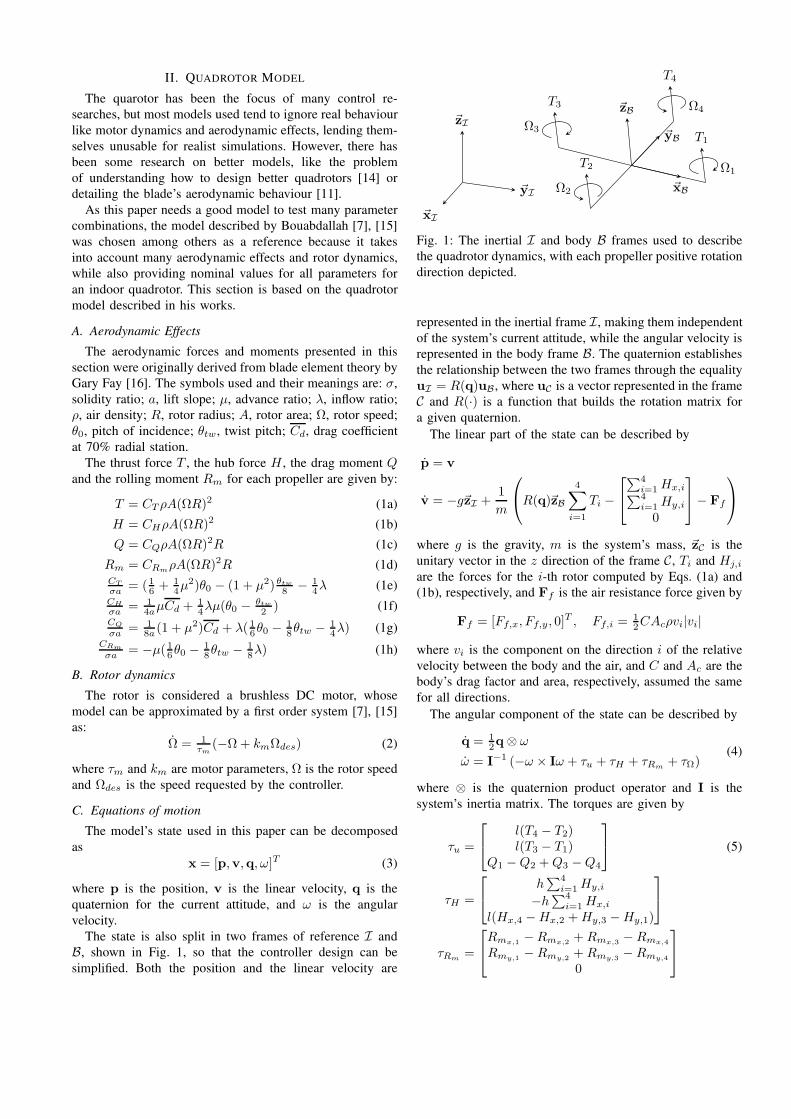
The state is also split in two frames of reference I and

B, shown in Fig. 1, so that the controller design can be

simplified. Both the position and the linear velocity are

~xI

~yI

~zI

~xB

~yB

~zB

T1

Ω1

T3

Ω3

T4

Ω4

T2

Ω2

Fig. 1: The inertial I and body B frames used to describe

the quadrotor dynamics, with each propeller positive rotation

direction depicted.

represented in the inertial frame I, making them independent

of the system’s current attitude, while the angular velocity is

represented in the body frame B. The quaternion establishes

the relationship between the two frames through the equality

uI = R(q)uB , where uC is a vector represented in the frame

C and R(·) is a function that builds the rotation matrix for

a given quaternion.

The linear part of the state can be described by

p = v

v = −g~zI +1

m

R(q)~zB

4∑

i=1

Ti −

∑4i=1Hx,i

∑4i=1Hy,i

0

− Ff

where g is the gravity, m is the system’s mass, ~zC is the

unitary vector in the z direction of the frame C, Ti and Hj,i

are the forces for the i-th rotor computed by Eqs. (1a) and

(1b), respectively, and Ff is the air resistance force given by

Ff = [Ff,x, Ff,y, 0]T , Ff,i =

12CAcρvi|vi|

where vi is the component on the direction i of the relative

velocity between the body and the air, and C and Ac are the

body’s drag factor and area, respectively, assumed the same

for all directions.

The angular component of the state can be described by

q = 12q⊗ ω

ω = I−1 (−ω × Iω + τu + τH + τRm + τΩ)(4)

where ⊗ is the quaternion product operator and I is the

system’s inertia matrix. The torques are given by

τu =

l(T4 − T2)l(T3 − T1)

Q1 −Q2 +Q3 −Q4

(5)

τH =

h∑4

i=1Hy,i

−h∑4i=1Hx,i

l(Hx,4 −Hx,2 +Hy,3 −Hy,1)

τRm =

Rmx,1 −Rmx,2 + Rmx,3 −Rmx,4Rmy,1 −Rmy,2 + Rmy,3 −Rmy,4

0

τΩ =

jrωyΩm−jrωxΩmjrΩm

, Ωm = Ω1 − Ω2 +Ω3 − Ω4

where l is the rotor arm length, h is the center of gravity’s

height, jr is the rotors’ inertia, ωi is the angular speed in the

direction i , Ωi is the i-th rotor speed computed by Eq. (2),

and Ti, Qi, Hj,i and Rmj,i are given by Eqs. (1a) to (1d).

III. BASE CONTROLLER

Consider that the controller must follow a trajectory given

by a reference position, pref (t), and reference rotation angle

around ~zI , ψref (t). [17] shows that all states and inputs

can be written algebraically based on these variables if the

model’s parameters are known, using it to design a trajectory

and a controller. A modified version of this controller is

presented in this section and will be used as the underlying

controller for the learning algorithm.

Although there are complex aerodynamic effects based on

the rotor speed, as shown in Sec. II, most controllers [5],

[6], [7], [10], [17], [18] consider only the thrust T and drag

moment Q from Eqs. (1a) and (1c), respectively, as inputs,

ignoring other aerodynamic effects or rotor dynamics. This

allows the designer to work with the torque τu from Eq. (5)

and a vertical thrust Fz . These efforts that can be transformed

in the propellers’ speed, assuming saturation doesn’t occur,

by solving the linear system

Fzτxτyτz

=

κT,1 κT,2 κT,3 κT,40 −lκT,2 0 lκT,4

−lκT,1 0 lκT,3 0κQ,1 −κQ,2 κQ,3 −κQ,4

︸ ︷︷ ︸

M

Ω21

Ω22

Ω23

Ω24

(6)

where the parameters κT,i and κQ,i can be found through

Eqs. (1a) and (1c) by setting Ti = κT,iΩ2i and Qi = κQ,iΩ

2i ,

and l is the rotor arm length.

Given the state decomposition in Eq. (3) and the trajectory

pref and ψref , an error state

e = [ep, ev, eq, eω]T (7)

can be defined, and the controller must be designed to reduce

these errors. As the position p is already defined by the

trajectory, the position and velocity errors are simply given

by ep = p− pref and ev = v − pref .

Let Kp and Kv be two positive definite matrices. Then a

PD force controller for the position is given by

Fdes = −Kpep −Kvev +mg~zI +mpref (8)

where m is the system’s mass, g is the gravity, pref is a

feedforward acceleration term, and ~zI is the unitary vector

in the z direction for the frame I, shown in Fig. 1.

As the quadrotor can only produce forces in the local

z direction using the thrusts Ti, the desired force Fdes,

assumed not null, must be decomposed in a scalar term

parallel to the body’s z axis, given by

Fz = Fdes · ~zB, (9)

where · is the scalar product, and a desired direction for the

z axis, given by

~zB,des =Fdes

‖Fdes‖. (10)

The angle ψref defines a rotation of the inertial frame Iaround ~zI , creating an intermediary coordinate frame C. The

x axis of this frame can be written as

~xC = [cosψref , sinψref , 0]T .

Using this frame and the desired body z direction given by

Eq. (10), the other axis for the desired frame are defined [17]

by

~yB,des =~zB,des × ~xC

‖~zB,des × ~xC‖, ~xB,des = ~yB,des × ~zB,des

if ~zB,des × ~xC 6= 0.

The three unitary vectors ~xB,des, ~yB,des, and ~zB,des define

a rotation matrix, from which a quaternion qdes can be

extracted using the method described in [19]. Using this

quaternion as a reference for q, the attitude error can be

written as

eq = q−1des ⊗ q. (11)

Let hω be defined by

hω =m

Fz(...pref − (~zB · ...

pref )~zB) , (12)

then the desired values for the angular speeds ωx and ωy are

given by

ωx,des = −hω · ~yB, ωy,des = hω · ~xB.

Finally, the desired value for ωz is given by

ωz,des = ψref~zI · ~zB,

and the angular speed error is defined as

eω = ω − ωdes (13)

Let kq be a positive scalar, Kω a positive definite matrix,

and ~eq the vector component of the error quaternion. Then

it can be shown [20] that the torque τ given by

τ = −kq~eq −Kωeω (14)

globally asymptotically stabilizes the attitude model in

Eq. (4) if τu = τ and only the gyroscopic effect is

considered. Stronger convergence guarantees can be given,

such as exponential stability or feedforward tracking, but

they require more knowledge about the system’s parameters,

like inertia values, which is precisely what this paper avoids.

It’s also important to note that qdes and ωdes aren’t constant,

so there’s no guarantee that the control law for τ will make

the system follow the trajectory with null error.

Using Fz and τ , defined in Eqs. (9) and (14), the rotor

speeds can be found using Eq. (6), assuming that the param-

eters κT and κQ are known.

IV. THE SIGNED DERIVATIVE ALGORITHM

Let a dynamic discrete system be described by

xt+1 = f(xt,ut), (15)

where xt is the state at time t and ut is a control input.

The controller design problem is defined by finding a set of

parameters θ so that the total path cost

J(x; θ) =

H∑

t=0

C(xt,ut), ut = π(xt; θ)

is minimized, where C(·, ·) is a cost function for a single

time step, π(·; ·) is the control policy, and H is the horizon

considered.

A simple algorithm to find the optimal parameter θ∗ is

the gradient descent, where θ is adjusted every H + 1 steps

in the reverse direction of the gradient. If the learn step is

given by α, then the adjustment can be written as

θk+1 = θk − α∂J(x; θk)

∂θk(16)

where the cost gradient is given by

∂J(x; θ)

∂θ=

H∑

t=0

(

(qt + rtKt)

(t−1∑

t′=0

∂xt∂ut′

Φt′

)

+ rtΦt

)

(17a)

qt ≡∂C(xt,ut)

∂xtrt ≡

∂C(xt,ut)

∂ut

Kt ≡∂π(xt; θ)

∂xtΦt ≡

∂π(xt; θ)

∂θ(17b)

Although the gradient depend mostly on known values,

defined through the known functions C(·, ·) and π(·; ·), the

partial derivative ∂xt∂ut′

measures the effect of ut′ on xt, which

depends on the dynamic model given by Eq. (15).

As the system’s model may not be known, Kolter [13],

[21] proposed that the partial derivative may be written as

∂xt∂ut′

= Dt(S+Et,t′) (18)

where Dt is a diagonal positive definite matrix and Et,t′ is an

error. Each line of the matrix S is given by at most one value

different of 0. This value must be +1 or −1, and encodes the

derivative’s sign for that state and input. Assuming that the

inputs are orthogonal, i.e., each state is affected mostly by a

single input, the matrix DtS provides a good approximation

for the derivative, as the lines of S can be scaled properly

to reduce the error matrix Et,t′ .

Kolter also notes in [21] that the lines of S may contain

more than one non-zero value, but their values must be in

the correct proportion, as the algorithm is unable to change

the columns scaling. This means that, if more than one

input affects significantly a state, the relative amount that

they change the state must be known or the error Et,t′ will

increase.

Using the approximate derivative given by Eq. (18), an

approximation to the gradient in Eq. (17a) can be written as

˜∂J(x; θ)

∂θ=

H∑

t=0

(

(qt + rtKt)S

(t−1∑

t′=0

Φt′

)

+ rtΦt

)

,

(19)

which depends only on the user knowledge about the system

embedded in S, and the cost and policy functions, also

defined by the user.

V. CONTROLLER OPTIMIZATION FOR A QUADROTOR

USING SIGNED DERIVATIVE

To use the signed derivative algorithm, the control policy

and cost function must be defined, so that the cost gradient in

Eq. (17a) can be computed. Moreover, the signed derivative

S must be built in a way as close as possible to the intended

format, and the motor saturation must be considered, as it

produces a discontinuity on the gradient.

A. Controller Policy

Although the controller output is given by the desired

rotor speeds, consider for now that it is actually given by

the vertical thrust Fz and torque τ .

It’s clear from Eqs. (8) and (12) that both Fz and τ depend

on the unknown system’s mass m. A standard approach in

adaptive control is to use one estimator for each use of

an unknown parameter [6], but the gradient terms∂π(xt;θ)

∂θ

for the feedforward acceleration pref and for hω would be

different from zero only when the system wasn’t hovering,

degrading their mass estimation. Although the mass term

associated with the gravity in Eq. (8) is always excited, it

isn’t capable of distinguishing changes in mass from vertical

wind changes. Hence a compromise of the uses of m must

be made to provide good estimation.

Consider that the state presented to the controller is the

error in Eq. (7), where the mass estimate is used instead of

the real value, and the vectors ~zI and ~zB are also given as

parameters independent of the state. The desired force Fdesfrom Eq. (8) can be written as

Fdes = θKpep + θKv

ev + θmg~zI +θmgg

pref , (20)

where θv is a controller’s parameter associated with the

original parameter v, and the perpendicular force Fz can be

computed using Eq. (9). The parameter θmg is used instead

of θm due to its higher value, providing more stability during

optimization. As θmg is used both to compensate gravity and

to improve feedforward tracking, the learnt parameter will

establish a compromise between the two while moving, and

focus on keeping altitude while hovering. This parameter is

also used in Eq. (12) instead of the correct mass to compute

hω.

Similarly to Fdes, the torque τ given by Eq. (14) can be

written as

τ = θkqeq + θKωeω + θτ (21)

where θτ is introduced to allow the torque to have a bias

on its value. As parameters for integral terms are hard to

learn, the varying bias serves as a replacement to reduce

static errors.

Once Fz and τ are computed, the rotors’ speeds can be

computed by Eq. (6). However, the transformation matrix

depends on many parameters, and κT and κQ aren’t even

constants. The dependency on l may be ignored by using

the scaled torques τ ′x = τx/l and τ ′y = τy/l in Eq. (21) and

letting the controller learn new parameters θ′.If the nominal thrust and drag coefficients for the propeller

are known, they are used instead of the correct values for

κT and κQ, which vary with the advance and inflow ratios.

If the nominal coefficients aren’t known, an approximation

matrix O(M) is used instead of M in Eq. (6), where

O(M) approximates the thrust and drag coefficients from

M by their orders of magnitude. While the effects of this

approximation are discussed in Sec. VII, it’s important to

note that M−1 corresponds to a right-hand multiplication of

S, thus making the columns scale incorrect and decreasing

performance if it differs from the real matrix.

The simplification of considering the error e as the state

known by the controller, with the directions ~zI and ~zB as

independent known parameters, reduces the complexity of

Φt, making the policy linear in the parameters, by avoiding

the computation of some intricate derivatives, like hω in

relation to θKp. However, it also decouples the linear and

angular systems originally coupled by Kt. This decoupling

doesn’t worsen the performance because, as discussed in the

next section, the value of Kt is ignored.

B. Cost Function

As suggested by Kolter [21], a common cost function is

given by the quadratic

C(x,u) = exTQex + eu

TReu (22)

where ex = x − xref and eu = u − uref are state and

control errors, respectively. These errors are computed using

some full state trajectory as reference, but such trajectory

generation algorithms generally use a known system’s model

to compute the desired states and inputs [17].

This approach isn’t feasible for the problem presented

in this paper, as the parameters are assumed unknown.

However, the state error given by Eq. (7), computed using

only pdes and ψdes as reference, can be used instead of the

error based on a previously determined full trajectory. As

for the control effort, it doesn’t have a reference value and

determining its cost may be hard, so R = 0 may be used

[21].

It’s important to notice that, by setting R = 0, the term

rt in Eq. (17a) is also null, making the gradient independent

of the value of Kt. Thus the simplification presented in the

last section, which decouples the linear and angular systems

from the controller policy’s perspective, affects the learning

only by approximating Φt. The only term that relates the two

subsystems is given by the matrix S.

C. Signed Derivative

As discussed in Sec. IV, the signed derivative S is built

based on the orthogonality between inputs. However, the

quadrotor is a well known under-actuated coupled dynamic

system, so its signed derivative must be designed to express

as much orthogonality as possible.

This design is greatly simplified by the observation that,

during the theoretical development in [21], the signed deriva-

tive S is assumed constant, but this constraint isn’t explored.

Indeed, S is isolated in Eq. (18), yielding

S = D−1t

∂xt∂ut′

−Et,t′ ,

and replaced in Eq. (19) for the analysis. Therefore, the

signed derivative can be generally described by a matrix

St,t′ .

While this general form increases the signed derivative

expressiveness, it also couples the times t and t′, which is

one of the main problems that the algorithm was designed

to solve. Therefore, an intermediary representation is con-

sidered in this paper, which allows the matrix S to vary

but restricts the time knowledge to a single time instant,

considering the state-output relationship to be approximately

constant in the horizon H . The two possibilities explored in

this paper are given by St and St′ , which will be computed

the same way but have slightly different meanings.

The matrix St establishes how previous inputs ut′ affect

the current state xt, assuming that the signed derivative

depends only on the current state. In contrast, the matrix St′

describes how future states xt will be affected by the current

input ut′ , such that the signed derivative in computed with

the state at the time of the input. Although the difference is

subtle and both resulting behaviours should be close if S is

continuous, they may differ significantly when the matrix is

discontinuous, as is the case of this work.

The signed derivative St can be decomposed as

St = [SpT ,Sp

T ,SqT ,Sω

T ]T ,

where Sc is the component for the state’s section c, and the

influence of the inputs over the position and linear velocity

is considered the same. The input order for the columns are

given by Fz , τx, τy and τz .

Assuming that the non-diagonal terms of the inertia matrix

I are small, it’s clear from Eq. (4) that each component of

the angular velocity ω is mainly affected by the respective

component of τ . As ω in the error computation, using

Eq. (13), is positive, the input affects the error eω in a similar

fashion. Therefore the matrix Sω can be defined as

Sω = [03×1, I3],

where 0 is the null matrix and I is the identity.

Consider now that the vector component for error quater-

nion ~eq is small, which makes the scalar component eq close

to ±1. A first order expansion of the quaternion dynamic in

Eq. (4) for the error in Eq. (11), assuming qdes constant, is

given by

eq,t+1 = eq,t +∆t

0eqωxeqωyeqωz

.

Using the relationship between ω and τ previously discussed,

the signed derivative can be written as

Sq =

[01×4

s(eq)Sω

]

,

where the function s(·) gives the sign of its argument.

Although the assumption of ~eq small may be invalid on

some cases, the controller is designed so that it is true most

of the time. Moreover, a generic formulation would have a

full matrix Sq, but the columns scaling is unknown as the

precise relation between ω and τ depends on the system’s

inertia.

For Sp, start with the assumption that the inertial I and

body B frames are aligned. In this case, it’s clear that epz is

mostly affected by Fz , incrementing epx requires τy to be

positive, and a negative value for τx increases epy . Assuming

that the inertias in the x and y directions have close values,

the proportion between τx and τy is next to 1 and the signed

derivative can have more than one non-zero term to mix

the effects of τx and τy without significantly increasing the

approximation error. Therefore, the general matrix Sp can

be written as

Sp =

0 sinψ cosψ 00 − cosψ sinψ 01 0 0 0

, (23)

where ψ is the rotation angle around ~zI between I and an

intermediary frame C′, which is given by the body frame

B with its z direction aligned to I. Note that this matrix

assumes that ~zI · ~zB > 0, as the inputs would have the

reverse effect otherwise. Hence a matrix Sp′ = s(~zI ·~zB)Sp

is used to allow the quadrotor to be facing down.

Note that the signed derivative Sp doesn’t consider the ef-

fect of Fz in the x and y directions, which can be significant

if the system’s attitude isn’t near hovering. Expressing such

knowledge depends on establishing a relationship between

the effects of Fz and τ so that the columns can be correctly

scaled, which isn’t trivial.

As the matrices Sq and Sp depend on certain assumptions

on the states, this can lead to incorrect learning when

violated. A solution for transient behaviours that may not

satisfy the assumptions is to disable learning by making

α = 0 in Eq. (16). However, the results in Sec. VII suggest

that the algorithm may be able to deal with these situations

by itself.

D. Dealing with Saturation

The efforts Fz and τ , computed through Eqs. (9), (20)

and (21), don’t take into consideration the motor saturation.

When solving Eq. (6) for Ω2i , the resulting values may

be unachievable by the rotors. In such cases, a common

practice is to just use the saturated value, though this leads

to a problem in the gradient defined in Eq. (17a), as the

derivatives in Eq. (17b) are ill defined. The solution to this

problem proposed in this paper is to ignore the gradient

gathered in this time window and start recollecting data as

if the horizon had been reached.

While the saturation may be a fluke in the system, it may

also be caused by the parameters θ being too big, which

makes the desired efforts large even for small errors. As this

may occur due to an overconfident previous learning step,

the parameters are adjusted with θk+1 = γθk whenever the

speeds saturate, in addition to resetting the gradient. The

parameter γ ≤ 1 controls how smooth is the parameters’ re-

duction, and must not be too low as the resulting parameters

may not be able to control the quadrotor.

VI. EXPERIMENTS

A. Simulation parameters

The parameters used on the simulations were separated in

three groups, with varying noise levels. The constant ones

are shown in Tab. I, and are comprised of literature values

for the model described in Sec. II and chosen simulation

parameters.

The learning rate α is small so that a larger horizon Hcan be used to better capture the dynamics, and to avoid

overconfident steps. As the learning is more conservative and

the rotor speed is considered to only be bounded from below,

due to the difficulty of finding upper bounds that always

allowed the quadrotor to even lift itself, the parameters shrink

γ wasn’t necessary. However, some experiments with the

nominal quadrotor parameters have shown that 0.99 < γ <0.999 greatly improves the performance during the initial

learning phase.

The cost matrix Q in Eq. (22) is decomposed as

Q = diag(qpI3, qvI3, 0, qqI3, qωI3),

where I3 is the identity matrix of size 3, and the scalar term

of the quaternion is assumed to have no cost, as its value is

adjusted based on the vector component. The input cost R

is considered null for the reasons discussed in Sec. V-B.

For the quadrotor parameters, the nominal values are

shown in Tabs. II and III. Each simulation parameter p′ is

created from the nominal one by applying a uniform noise,

such that p′ = p(1 +wp), wp ∼ U([−β, β]), where p is the

nominal value and β is the noise level.

The parameters in Tab. II have smaller values of β as

they aren’t actually independent [16]. Also, by examining

Eqs. (1e) to (1h), it’s clear that incorrect values may affect

the results significantly. For instance, in Eq. (1e), if θ0 gets

smaller while θtw gets bigger, the thrust coefficient may

become negative, which means that a positive rotor speed

produces thrust in the reverse direction. This effect was

perceived for lager values of β, which lead to the reduced

noise level. It’s also important to highlight that the noisy

values may not correspond to any real propeller, as these

usually have their parameters optimized, and may not be

a good fit for the quadrotor’s parameters, which influence

which propeller is chosen, hence the performance may be

worsened.

The matrix M in Eq. (6) depend on the nominal simulation

values κ′T and κ′Q, as discussed in Sec. V-A. As those values

may not be available, the notion of approximating M by

a matrix with the order of magnitude of its terms O(M)

TABLE I: Constant experiment parameters.

Parameter Description Value

a Lift slope 5.7ρ Air density 1.293

Number of blades 2g Gravity 9.81

Number of runs 100Simulated time in seconds 120

Sampling frequency in hertz 1000α Learning rate 10−4

H Learning horizon 9γ Parameter shrink on saturation 1Ω Maximum rotor speed ∞

Ω Minimum rotor speed 0qp Position cost 1qv Linear velocity cost 1qq Quaternion cost 10qω Angular velocity cost 1

TABLE II: Propeller parameters with β = 0.1.

Parameter Description Value

θ0 Pitch of incidence 0.2618θtw Twist picth 0.045Cd Drag coefficient 0.052c Chord 0.0394R Radius 0.15

TABLE III: Experiment parameters with β = 0.25.

Parameter Description Value

km Rotor gain 0.936τm Rotor time constant 0.178I Quadrotor’s inertia diag([7.5, 7.5, 1.3])× 10−3

κT Nominal thrust coefficient 3.13× 10−5

κQ Nominal drag coefficient 7.5× 10−7

l Arm length 0.232m Mass 0.53jr Rotor inertia 6× 10−5

h Center of gravity’s height 0.058Ac Center hub area 0.005C Center drag coefficient 1.32

was introduced. Experiments have shown that starting with

a controller overconfident of how much thrust and drag the

propellers produce provides better results than otherwise, as

the lower rotor speeds are applied. Therefore, the parameters

κ′i are approximated by O(κi) = 10⌈log10 κi⌉, where ⌈·⌉ is

the round up operator, and the original nominal value is used

instead of the nominal noised one, which is assumed to be

unknown.

Besides the noisy parameters, a small wind was also

applied during simulation, as the nominal parameters are

from an indoor quadrotor [15]. The wind wt at time step

t is composed of two different sources such that wt =wt,1 + wt,2. The first one describes fast change in wind,

due to rotor motion and to simulate natural vibration, and is

described by wt,1 ∼ N (03×1, 0.5I3), where N (µ, σ) is the

normal distribution, while the second one is a dynamic wind

flow characterized by wt,2 =√1− τ2wt−1,2 + τvt,vt ∼

N (03×1, 0.1I3), where the time constant is τ = 10−3 and

the starting condition is w0,2 ∼ N (03×1, 0.1I3).

The controller parameters in Eqs. (20) and (21) are as-

sumed to be diagonal, and their initial values are given by

θKp= −2I3, θKv

= −5I3, θKq= −10, θKω

= −I3, and

θmg = 0, where I3 is the identity matrix of size 3 and θmgstarts null as no mass estimate is used.

B. Learning methodology

As the initial value for θmg is null, the quadrotor isn’t

even able to hover. The first step in the learning process is

to find some good initial estimate so that the vehicle can be

near hover. This is achieved by starting at an initial position

on the ground, such that pz ≥ 0, setting θmg = 10t, where tis the current time, and only using it to compute the control

output. Once pz > 0, the vehicle has taken flight and the

current value of θmg is used as initial estimate for the next

phase. It must be highlighted that, in general, this estimate

is higher than the value needed for hovering due to rotor

dynamics, as described by Eq. (2).

Once the initial θmg has been estimated, the quadrotor

is left on the air with its motors shutdown at the desired

position and orientation, so that it can adjust its parameters

to have good hovering values.

The final step is composed of circular trajectories which

are given by

pref (t) = [rT cos(ωT t), rT sin(ωT t), 0]T , ψref (t) = ωT t.

(24)

To avoid large control values due to non-zero initial error

and to test the performance on inconsistent trajectories, the

values derived from the trajectory used by the controller are

given by

v′ref =

vrefttw, if t ≤ tw

vref , otherwise

where tw is the time window to reach the original trajectory,

such that larger values provide a smoother transition but the

trajectory is inconsistent for longer time periods, and v is

any trajectory derived value used by the controller, such as...p.

VII. RESULTS

There are two different sets of results in this paper. The

first one assumes that the nominal noisy propeller parameters

κ′T and κ′Q are known, so that the matrix M in Eq. (6)

is closer to the real one. The second set assumes that

these parameters aren’t available, and are replaced by their

approximations O(κi).The legend t corresponds to learning using St, while

t′ corresponds to using St′ , where the difference between

the two is discussed in Sec. V-C. The heading angle ψ is

computed from the attitude q considering only a rotation

around z, while the heading error is given by eψ = ψ−ψref .

A. Known propeller parameters

Figure 2 shows the quadrotor performance during hover.

It’s clear that in the first few seconds the controller is

getting used to the dynamics, adjusting the parameters ag-

gressively. Nonetheless, the position stayed within reasonable

boundaries, suggesting that this first learning can happen

in any available space. The signed derivative St had faster

0 20 40 60 80 100 120−4

−2

0

2

4

6

8

tt′

ψ(

)

Time (s)0 20 40 60 80 100 120

−0.15

−0.1

−0.05

0

0.05

0.1

0.15

0.2

tt′

px

(m)

Time (s)

0 20 40 60 80 100 120−0.8

−0.6

−0.4

−0.2

0

0.2

0.4

0.6

0.8

tt′

py

(m)

Time (s)0 20 40 60 80 100 120

−0.4

−0.2

0

0.2

0.4

0.6

0.8

1

tt′

pz

(m)

Time (s)

Fig. 2: Upper and lower bounds while hovering with correct parameters, and two options of S.

0 20 40 60 80 100 120−200

−100

0

100

200

0 20 40 60 80 100 120−20

−15

−10

−5

0

5

10

tt′

ψ(

)eψ

()

Time (s)

0 20 40 60 80 100 120−3

−2

−1

0

1

2

3

0 20 40 60 80 100 120−1.5

−1

−0.5

0

0.5

1

1.5

tt′

px

(m)

epx

(m)

Time (s)

0 20 40 60 80 100 120−3

−2

−1

0

1

2

3

0 20 40 60 80 100 120−1.5

−1

−0.5

0

0.5

1

1.5

tt′

py

(m)

epy

(m)

Time (s)0 20 40 60 80 100 120

−1

−0.5

0

0.5

1

1.5

2

tt′

pz

(m)

Time (s)

Fig. 3: Upper and lower bounds for circular trajectory with rT = 2, ωT = 2π4 , tw = 10, correct

parameters, and two options of S.

convergence than its counterpart S′t on some cases, but both

performed similarly most of the time.

It’s worth noting that the boundaries for x and y are

practically constant, presenting minor oscillations. Although

the error is small, it shows a flaw in the controller that must

be kept in mind: the signed derivative in Eq. (23) doesn’t

0 20 40 60 80 100 120−200

−100

0

100

200

0 20 40 60 80 100 120−10

−8

−6

−4

−2

0

2

4

tt′

ψ(

)eψ

()

Time (s)

0 20 40 60 80 100 120−4

−2

0

2

4

6

0 20 40 60 80 100 120−2

−1.5

−1

−0.5

0

0.5

1

1.5

tt′

px

(m)

epx

(m)

Time (s)

0 20 40 60 80 100 120−6

−4

−2

0

2

4

0 20 40 60 80 100 120−2

−1.5

−1

−0.5

0

0.5

1

1.5

tt′

py

(m)

epy

(m)

Time (s)0 20 40 60 80 100 120

−1

−0.5

0

0.5

1

1.5

2

2.5

tt′

pz

(m)

Time (s)

Fig. 4: Upper and lower bounds for circular trajectory with rT = 4, ωT = 2π8 , tw = 20, correct

parameters, and two options of S.

0 20 40 60 80 100 120−5

−4

−3

−2

−1

0

1

2

3

4

5

tt′

ψ(

)

Time (s)0 20 40 60 80 100 120

−0.6

−0.4

−0.2

0

0.2

0.4

0.6

0.8

tt′

px

(m)

Time (s)

0 20 40 60 80 100 120−0.5

−0.4

−0.3

−0.2

−0.1

0

0.1

0.2

0.3

0.4

0.5

tt′

py

(m)

Time (s)0 20 40 60 80 100 120

−1

−0.5

0

0.5

1

1.5

tt′

pz

(m)

Time (s)

Fig. 5: Upper and lower bounds while hovering with approximate parameters and two options of

S.

express any relation between Fz and the position on x and

y due to limitations discussed in Sec. V-C. Therefore, the

controller seem to be able to compensate for lateral wind

only by applying some torque to prevent the quadrotor from

0 20 40 60 80 100 120−200

−100

0

100

200

0 20 40 60 80 100 120−30

−20

−10

0

10

20

tt′

ψ(

)eψ

()

Time (s)

0 20 40 60 80 100 120−4

−2

0

2

4

0 20 40 60 80 100 120−4

−3

−2

−1

0

1

2

tt′

px

(m)

epx

(m)

Time (s)

0 20 40 60 80 100 120−6

−4

−2

0

2

4

0 20 40 60 80 100 120−3

−2

−1

0

1

2

3

tt′

py

(m)

epy

(m)

Time (s)0 20 40 60 80 100 120

−1.5

−1

−0.5

0

0.5

1

1.5

2

2.5

3

tt′

pz

(m)

Time (s)

Fig. 6: Upper and lower bounds for circular trajectory with rT = 2, ωT = 2π5 , tw = 10, approximate

parameters, and two options of S.

0 20 40 60 80 100 120−200

−100

0

100

200

0 20 40 60 80 100 120−8

−6

−4

−2

0

2

4

6

tt′

ψ(

)eψ

()

Time (s)

0 20 40 60 80 100 120−5

0

5

0 20 40 60 80 100 120−4

−2

0

2

4

tt′

px

(m)

epx

(m)

Time (s)

0 20 40 60 80 100 120−5

0

5

0 20 40 60 80 100 120−2

−1

0

1

2

3

4

5

tt′

py

(m)

epy

(m)

Time (s)0 20 40 60 80 100 120

−1.5

−1

−0.5

0

0.5

1

1.5

2

2.5

3

3.5

tt′

pz

(m)

Time (s)

Fig. 7: Upper and lower bounds for circular trajectory with rT = 4, ωT = 2π10 , tw = 20, approximate

parameters, and two options of S.

drifting. However, as the errors in pz are significantly higher,

due to its higher sensitivity to wind, and every position’s

component has the same weight, the controller focus most

of its effort on the altitude.

Figures 3 and 4 show the controller following two different

circular trajectories described by Eq. (24) after learning the

hovering parameters. Even though the underlying controller

is simple, being composed basically of PD controllers with

no angular feedforward, the signed derivative doesn’t have

correct columns scaling, and the propeller parameters may

not be adequate, the learnt parameters allow the vehicle to

follow the trajectory reasonably well.

B. Approximate propeller parameters

Figure 5 shows the controller learning to hover a quadrotor

without any parameter knowledge. Although the errors dur-

ing the first few seconds are higher than the previous case,

the performance after the parameters have nearly converged

is similar to the one presented in Fig. 2. This occurs because,

during hover, the main control effort used is the force

Fz , with the torques near zero, so that the rotors’ speed

coupling isn’t strong. In this situation, O(M) is clearly a

good approximation.

However, the approximation degrades the performance

during highly coupled trajectories, such as the circular ones

in Figs. 6 and 7. In these, the controller isn’t much capable

of dealing with the trajectory inconsistencies during the

initial window, leading to large transient errors. The rotation

speed was lowered from the previous case as the transient

inconsistency on the original speed destabilized the system.

Even though the steady lateral errors also increase, the

vehicle follows the trajectory close enough for some appli-

cations, and is kept stable even with the gradient direction

considerably distorted. Although not presented here, using

unmodified propeller parameters, i.e., setting β = 0 for the

values in Tab. II, the errors are reduced in half, indicating

that the values assigned may not be used in real systems and

the real error may be considerably smaller with appropriate

components choice.

From the position px in Fig. 7 at t = 40, 50, 60, . . .,it’s obvious that the errors aren’t consistent each turn. This

is a result of the incorrect gradient, as the controller tries

to minimize the total error and may end up increasing it.

However, the trajectory is aggressive enough that a static

controller, with the parameters learnt during hover, isn’t able

to stabilize the system. As the learning algorithm searches for

the locally optimal solution, it’s able to change its parameter

settings based on the local error, thus forming a dynamic

system on itself.

VIII. CONCLUSION

This paper presented a simple PD-based controller to stabi-

lize a quadrotor without parameters knowledge using signed

derivative policy iteration. Two approaches were analysed,

where they differed on whether the controller knows only the

nominal propeller parameters or an approximation is used.

Even though the gradient is distorted due to the signed

derivative having incorrect columns scaling, which is a

limitation of the technique, the controller ignores rotor

dynamics and most aerodynamic effects, and doesn’t use

angular feedforward, the vehicle achieved stable hovering

and was able to follow a circular trajectory. However, if

the propeller parameters are unknown, the error on fast

trajectories may be too large for some applications. To the

best of the authors’ knowledge, this is the first quadrotor

controller proposal that requires no parameter knowledge or

hand tunning whatsoever.

If the nominal propeller parameters are known, the per-

formance may be further improved if the position signed

derivative is aware of how the thrust affects the x and ypositions, while keeping the torque knowledge. For the case

where no parameters are known, knowing the ratio between

the propeller parameters may also boost performance. As

the signed derivative isn’t able to learn these parameters,

an approach currently being studied is the use of another

learning algorithm to learn these scalings online.

Simulations have shown that the quadrotor’s transient

behaviour may distance significantly from the desired tra-

jectory. As safety is a major concern for these systems [22],

one may be able to apply reachability sets [23] to disable

learning and switch to a safe controller if necessary. Also,

if the task performed is repetitive, other approaches such as

iterative learning control [24] and trajectory corrections [25],

[26] can also be integrated to compensate for errors caused

by policy iteration limitations, although the effects of this

simultaneous learning are still being analysed.

REFERENCES

[1] S. Lupashin, A. Schollig, M. Hehn, and R. D’Andrea, “The flyingmachine arena as of 2010,” in Proceedings of the IEEE International

Conference on Robotics and Automation. IEEE, 2011, pp. 2970–2971.

[2] G. M. Hoffmann, D. G. Rajnarayan, S. L. Waslander, D. Dostal, J. S.Jang, and C. J. Tomlin, “The Stanford testbed of autonomous rotorcraftfor multi agent control (STARMAC),” in Digital Avionics Systems

Conference. IEEE, 2004.

[3] S. Bouabdallah, P. Murrieri, and R. Siegwart, “Design and control ofan indoor micro quadrotor,” in Proceedings of the IEEE International

Conference on Robotics and Automation. IEEE, 2004, pp. 4393–4398,vol. 5.

[4] A. Benallegue, A. Mokhtari, and L. Fridman, “High-order sliding-mode observer for a quadrotor UAV,” International Journal of Robust

and Nonlinear Control, vol. 18, no. 4-5, pp. 427–440, 2008.

[5] T. Madani and A. Benallegue, “Backstepping control for a quadrotorhelicopter,” in Proceedings of the IEEE International Conference on

Intelligent Robots and Systems. IEEE, Oct. 2006, pp. 3255–3260.

[6] M. Huang, B. Xian, C. Diao, K. Yang, and Y. Feng, “Adaptivetracking control of underactuated quadrotor unmanned aerial vehiclesvia backstepping,” in American Control Conference. IEEE, 2010, pp.2076–2081.

[7] S. Bouabdallah and R. Siegwart, “Full control of a quadrotor,” inProceedings of the IEEE International Conference on IntelligentRobots and Systems, no. 1. IEEE, Oct. 2007, pp. 153–158.

[8] L. Besnard, Y. B. Shtessel, and B. Landrum, “Quadrotor vehiclecontrol via sliding mode controller driven by sliding mode disturbanceobserver,” Journal of the Franklin Institute, vol. 349, no. 2, pp. 658–684, Mar. 2012.

[9] S. Bouabdallah, A. Noth, and R. Siegwart, “PID vs LQ controltechniques applied to an indoor micro quadrotor,” in Proceedings of

the IEEE International Conference on Intelligent Robots and Systems,vol. 3. IEEE, 2004, pp. 2451–2456, vol. 3.

[10] P. E. I. Pounds, R. Mahony, and P. Corke, “Modelling and control ofa large quadrotor robot,” Control Engineering Practice, vol. 18, no. 7,pp. 691–699, July 2010.

[11] G. M. Hoffmann, H. Huang, S. L. Waslander, and C. J. Tomlin,“Quadrotor helicopter flight dynamics and control: Theory and experi-ment,” in Proceedings of the AIAA Guidance, Navigation, and Control

Conference, no. August. AIAA, 2007, pp. 1–20.

[12] A. Y. Ng, H. J. Kim, M. I. Jordan, and S. Sastry, “Autonomoushelicopter flight via Reinforcement Learning,” in Advances in NeuralInformation Processing Systems 16, vol. Volume 21. MIT Press,2004.

[13] J. Kolter and A. Ng, “Policy search via the signed derivative,” inRobotics: science and systems. MIT Press, 2009.

[14] P. E. I. Pounds, R. Mahony, J. Gresham, P. Corke, and J. Roberts,“Towards dynamically-favourable quad-rotor aerial robots,” in Pro-

ceedings of the 2004 Australasian Conference on Robotics and Au-tomation. ARAA, 2004.

[15] S. Bouabdallah, “Design and control of quadrotors with application toautonomous flying,” Ph.D. dissertation, 2007.

[16] G. Fay, “Derivation of the aerodynamic forces for the mesicoptersimulation,” Stanford University, Tech. Rep., 2001.

[17] D. Mellinger and V. Kumar, “Minimum snap trajectory generationand control for quadrotors,” in Proceedings of the IEEE InternationalConference on Robotics and Automation. IEEE, 2011, pp. 2520–2525.

[18] N. Guenard, T. Hamel, and V. Moreau, “Dynamic modeling andintuitive control strategy for an X4-flyer,” in Proceedings of the IEEE

International Conference on Control and Automation. IEEE, 2005,pp. 141–146, vol. 1.

[19] I. Y. Bar-Itzhack, “New method for extracting the quaternion from arotation matrix,” Journal of Guidance, Control, and Dynamics, vol. 23,no. 6, pp. 1085–1087, 2000.

[20] A. Tayebi and S. McGilvray, “Attitude stabilization of a four-rotoraerial robot,” in Conference on Decision and Control. IEEE, 2004,pp. 1216–1221, vol. 2.

[21] J. Z. Kolter, “Learning and control with inaccurate models,” Ph.D.dissertation, 2010.

[22] M. W. Mueller and R. D’Andrea, “Critical subsystem failure mitigationin an indoor UAV testbed,” in Proceedings of the IEEE InternationalConference on Intelligent Robots and Systems. IEEE, Oct. 2012, pp.780–785.

[23] J. H. Gillula and C. J. Tomlin, “Reducing Conservativeness in SafetyGuarantees by Learning Disturbances Online: Iterated Guaranteed SafeOnline Learning.” in Robotics: Science and Systems. IEEE, 2012.

[24] O. Purwin and R. D’Andrea, “Performing aggressive maneuvers usingiterative learning control,” in Proceedings of the IEEE InternationalConference on Robotics and Automation. IEEE, May 2009, pp. 1731–1736.

[25] S. Lupashin, A. Schollig, M. Sherback, and R. D’Andrea, “A simplelearning strategy for high-speed quadrocopter multi-flips,” in Pro-

ceedings of the IEEE International Conference on Robotics and

Automation. IEEE, 2010, pp. 1642–1648.[26] S. Lupashin and R. D’Andrea, “Adaptive open-loop aerobatic maneu-

vers for quadrocopters,” in IFAC World Congress, no. 2010. IFAC,2011, pp. 2600–2606.