Qu: 00, 00, 00, 00 - Apache2 Ubuntu Default Page: It works GHA/LOW P2: FQP Final Qu: 00, 00, 00, 00...

P1: GHA/LOW P2: FQP Final Qu: 00, 00, 00, 00

Encyclopedia of Physical Science and Technology EN006C-258 June 28, 2001 19:56

Fourier SeriesJames S. WalkerUniversity of Wisconsin–Eau Claire

I. Historical BackgroundII. Definition of Fourier SeriesIII. Convergence of Fourier SeriesIV. Convergence in NormV. Summability of Fourier Series

VI. Generalized Fourier SeriesVII. Discrete Fourier Series

VIII. Conclusion

GLOSSARY

Bounded variation A function f has bounded vari-ation on a closed interval [a, b] if there exists apositive constant B such that, for all finite setsof points a = x0 < x1 < · · · < xN = b, the inequality∑N

i=1 |f(xi ) − f(xi−1)| ≤ B is satisfied. Jordan provedthat a function has bounded variation if and only if itcan be expressed as the difference of two nondecreas-ing functions.

Countably infinite set A set is countably infinite if itcan be put into one-to-one correspondence with the setof natural numbers (1, 2, . . . , n, . . .). Examples: Theintegers and the rational numbers are countably infinitesets.

Continuous function If limx→cf(x) = f(c), then the func-tion f is continuous at the point c. Such a point is calleda continuity point for f. A function which is continuousat all points is simply referred to as continuous.

Lebesgue measure zero A set S of real numbers is said tohave Lebesgue measure zero if, for each ε > 0, there ex-

ists a collection {(ai , bi )}∞i=1 of open intervals such thatS ⊂ ∪∞

i=1(ai , bi ) and∑∞

i=1(bi − ai ) ≤ ε. Examples: Allfinite sets, and all countably infinite sets, have Lebesguemeasure zero.

Odd and even functions A function f is odd iff(−x) = −f(x) for all x in its domain. A function f iseven if f(−x) = f(x) for all x in its domain.

One-sided limits f(x−) and f(x+) denote limits of f(t)as t tends to x from the left and right, respectively.

Periodic function A function f is periodic, with periodP > 0, if the identity f(x + P) = f(x) holds for all x .Example: f(x) = | sin x | is periodic with period π .

FOURIER SERIES has long provided one of the prin-cipal methods of analysis for mathematical physics, en-gineering, and signal processing. It has spurred general-izations and applications that continue to develop rightup to the present. While the original theory of Fourierseries applies to periodic functions occurring in wave mo-tion, such as with light and sound, its generalizations often

167

html

P1: GHA/LOW P2: FQP Final


168 Fourier Series

relate to wider settings, such as the time-frequency analy-sis underlying the recent theories of wavelet analysis andlocal trigonometric analysis.

I. HISTORICAL BACKGROUND

There are antecedents to the notion of Fourier series inthe work of Euler and D. Bernoulli on vibrating strings,but the theory of Fourier series truly began with the pro-found work of Fourier on heat conduction at the begin-ning of the 19th century. Fourier deals with the problemof describing the evolution of the temperature T (x, t) of athin wire of length π , stretched between x = 0 and x = π ,with a constant zero temperature at the ends: T (0, t) = 0and T (π, t) = 0. He proposed that the initial tempera-ture T (x, 0) = f(x) could be expanded in a series of sinefunctions:

f(x) =∞∑

n=1

bn sin nx (1)

with

bn = 2

π

∫ π

0f(x) sin nx dx . (2)

A. Fourier Series

Although Fourier did not give a convincing proof of con-vergence of the infinite series in Eq. (1), he did offer theconjecture that convergence holds for an “arbitrary” func-tion f. Subsequent work by Dirichlet, Riemann, Lebesgue,and others, throughout the next two hundred years, wasneeded to delineate precisely which functions wereexpandable in such trigonometric series. Part of this workentailed giving a precise definition of function (Dirichlet),and showing that the integrals in Eq. (2) are properlydefined (Riemann and Lebesgue). Throughout this articlewe shall state results that are always true when Riemannintegrals are used (except for Section IV where we needto use results from the theory of Lebesgue integrals).

In addition to positing Eqs. (1) and (2), Fourier arguedthat the temperature T (x, t) is a solution to the followingheat equation with boundary conditions:

∂T

∂t= ∂2T

∂x2, 0 < x < π, t > 0

T (0, t) = T (π, t) = 0, t ≥ 0

T (x, 0) = f (x), 0 ≤ x ≤ π.

Making use of Eq. (1), Fourier showed that the solutionT (x, t) satisfies

T (x, t) =∞∑

n=1

bne−n2t sin nx . (3)

This was the first example of the use of Fourier series tosolve boundary value problems in partial differential equa-tions. To obtain Eq. (3), Fourier made use of D. Bernoulli’smethod of separation of variables, which is now a stan-dard technique for solving boundary value problems.

A good, short introduction to the history of Fourier se-ries can be found in The Mathematical Experience. Be-sides his many mathematical contributions, Fourier hasleft us with one of the truly great philosophical principles:“The deep study of nature is the most fruitful source ofknowledge.”

II. DEFINITION OF FOURIER SERIES

The Fourier sine series, defined in Eqs. (1) and (2), is a spe-cial case of a more general concept: the Fourier series for aperiodic function. Periodic functions arise in the study ofwave motion, when a basic waveform repeats itself peri-odically. Such periodic waveforms occur in musical tones,in the plane waves of electromagnetic vibrations, and inthe vibration of strings. These are just a few examples.Periodic effects also arise in the motion of the planets, inAC electricity, and (to a degree) in animal heartbeats.

A function f is said to have period P if f(x + P) =f(x) for all x . For notational simplicity, we shall restrictour discussion to functions of period 2π . There is no lossof generality in doing so, since we can always use a sim-ple change of scale x = (P/2π )t to convert a function ofperiod P into one of period 2π .

If the function f has period 2π , then its Fourier series is

c0 +∞∑

n=1

{an cos nx + bn sin nx} (4)

with Fourier coefficients c0, an , and bn defined by theintegrals

c0 = 1

2π

∫ π

−π

f(x) dx (5)

an = 1

π

∫ π

−π

f(x) cos nx dx, (6)

bn = 1

π

∫ π

−π

f(x) sin nx dx . (7)

[Note: The sine series defined by Eqs. (1) and (2) is aspecial instance of Fourier series. If f is initially definedover the interval [0, π ], then it can be extended to [−π, π ](as an odd function) by letting f(−x) = −f(x), and thenextended periodically with period P = 2π . The Fourierseries for this odd, periodic function reduces to the sineseries in Eqs. (1) and (2), because c0 = 0, each an = 0, andeach bn in Eq. (7) is equal to the bn in Eq. (2).]



Fourier Series 169

It is more common nowadays to express Fourier se-ries in an algebraically simpler form involving complexexponentials. Following Euler, we use the fact that thecomplex exponential ei θ satisfies ei θ = cos θ + isin θ .Hence

cos θ = 1

2(ei θ + ei θ ),

sin θ = 1

2i (ei θ − e −i θ ).

From these equations, it follows by elementary algebrathat Formulas (5)–(7) can be rewritten (by rewriting eachterm separately) as

c0 +∞∑

n =1

{cneinx + c−ne −inx

}(8)

with cn defined for all integers n by

cn = 1

2π

∫ π

−π

f(x)e −inx dx . (9)

The series in Eq. (8) is usually written in the form

∞∑n =−∞

cneinx . (10)

We now consider a couple of examples. First, let f1 bedefined over [−π, π ] by

f1(x) ={

1 if |x | < π/2

0 if π/2 ≤ |x | ≤ π

and have period 2π . The graph of f1 is shown in Fig. 1;it is called a square wave in electric circuit theory. Theconstant c0 is

c0 = 1

2π

∫ π

−π

f1(x) dx

= 1

2π

∫ π/2

−π/21 dx = 1

2 .

While, for n �= 0,

cn = 1

2π

∫ π

−π

f1(x)e −inx dx

= 1

2π

∫ π/2

−π/2e −inx dx

= 1

2π

e −inπ/2 − einπ/2

−in

= sin(n π/2)

n π.

FIGURE 1 Square wave.

Thus, the Fourier series for this square wave is

1

2+

∞∑n=1

sin(nπ/2)

nπ(einx + e−inx )

= 1

2+

∞∑n=1

2 sin(nπ/2)

nπcos nx . (11)

Second, let f2(x) = x2 over [−π, π] and have period 2π ,see Fig. 2. We shall refer to this wave as a parabolic wave.This parabolic wave has c0 = π2/3 and cn , for n �= 0, is

cn = 1

2π

∫ π

−π

x2e−inx dx

= 1

2π

∫ π

−π

x2 cos nx dx − i

2π

∫ π

−π

x2 sin nx dx

= 2(−1)n

n2

after an integration by parts. The Fourier series for thisfunction is then

π2

3+

∞∑n=1

2(−1)n

n2(einx + e−inx )

= π2

3+

∞∑n=1

4(−1)n

n2cos nx . (12)

We will discuss the convergence of these Fourier series,to f1 and f2, respectively, in Section III.



170 Fourier Series

FIGURE 2 Parabolic wave.

Returning to the general Fourier series in Eq. (10), weshall now discuss some ways of interpreting this series. Acomplex exponential einx = cos nx + isin nx has a small-est period of 2π/n. Consequently it is said to have a fre-quency of n/2π , because the form of its graph over theinterval [0, 2π/n] is repeated n/2π times within each unit-length. Therefore, the integral in Eq. (9) that defines theFourier coefficient cn can be interpreted as a correlationbetween f and a complex exponential with a precisely lo-cated frequency of n/2π . Thus the whole collection ofthese integrals, for all integers n, specifies the frequencycontent of f over the set of frequencies {n/2π}∞n=−∞. Ifthe series in Eq. (10) converges to f, i.e., if we can write

f(x) =∞∑

n=−∞cneinx , (13)

then f is being expressed as a superposition of elemen-tary functions cneinx having frequency n/2π and ampli-tude cn . (The validity of Eq. (13) will be discussed in thenext section.) Furthermore, the correlations in Eq. (9) areindependent of each other in the sense that correlationsbetween distinct exponentials are zero:

1

2π

∫ π

−π

einx e−imx dx ={

0 if m �= n

1 if m = n.(14)

This equation is called the orthogonality property of com-plex exponentials.

The orthogonality property of complex exponentialscan be used to give a derivation of Eq. (9). Multiplying

Eq. (13) by e−imx and integrating term-by-term from −π

to π , we obtain

∫ π

−π

f(x)e−imx dx =∞∑

n=−∞cn

∫ π

−π

einx e−imx dx .

By the orthogonality property, this leads to∫ π

−π

f(x)e−imx dx = 2πcm,

which justifies (in a formal, nonrigorous way) the defini-tion of cn in Eq. (9).

We close this section by discussing two important prop-erties of Fourier coefficients, Bessel’s inequality and theRiemann-Lebesgue lemma.

Theorem 1 (Bessel’s Inequality): If∫ π

−π|f(x)|2 dx is fi-

nite, then

∞∑n=−∞

|cn|2 ≤ 1

2π

∫ π

−π

|f(x)|2 dx . (15)

Bessel’s inequality can be proved easily. In fact, we have

0 ≤ 1

2π

∫ π

−π

∣∣∣∣∣f(x) −N∑

n=−N

cneinx

∣∣∣∣∣2

dx

= 1

2π

∫ π

−π

(f(x) −

N∑m=−N

cmeimx

)(f(x) −

N∑n=−N

cne−inx

)dx .

Multiplying out the last integrand above, and making useof Eqs. (9) and (14), we obtain

1

2π

∫ π

−π

∣∣∣∣∣f(x) −N∑

n=−N

cneinx

∣∣∣∣∣2

dx

= 1

2π

∫ π

−π

|f(x)|2 dx −N∑

n=−N

|cn|2. (16)

Thus, for all N ,

N∑n=−N

|cn|2 ≤ 1

2π

∫ π

−π

|f(x)|2 dx (17)

and Bessel’s inequality (15) follows by letting N → ∞.

Bessel’s inequality has a physical interpretation. If f hasfinite energy, in the sense that the right side of Eq. (15) isfinite, then the sum of the moduli-squared of the Fouriercoefficients is also finite. In Section IV, we shall see thatthe inequality in Eq. (15) is actually an equality, whichsays that the sum of the moduli-squared of the Fouriercoefficients is precisely the same as the energy of f.



Fourier Series 171

Because of Bessel’s inequality, it follows that

lim|n |→∞

cn = 0 (18)

holds whenever∫ π

−π|f(x)|2 dx is finite. The Riemann-

Lebesgue lemma says that Eq. (18) holds in the followingmore general case:

Theorem 2 (Riemann-Lebesgue Lemma): If∫ π

−π| f(x)| dx is finite, then Eq. (18) holds.

One of the most important uses of the Riemann-Lebesguelemma is in proofs of some basic pointwise convergencetheorems, such as the ones described in the next section.

See Krantz and Walker (1998) for further discussionsof the definition of Fourier series, Bessel’s inequality, andthe Riemann-Lebesgue lemma.

III. CONVERGENCE OF FOURIER SERIES

There are many ways to interpret the meaning of Eq. (13).Investigations into the types of functions allowed on theleft side of Eq. (13), and the kinds of convergence con-sidered for its right side, have fueled mathematical in-vestigations by such luminaries as Dirichlet, Riemann,Weierstrass, Lipschitz, Lebesgue, Fejer, Gelfand, andSchwartz. In short, convergence questions for Fourier se-ries have helped lay the foundations and much of the su-perstructure of mathematical analysis.

The three types of convergence that we shall describehere are pointwise, uniform, and norm convergence. Weshall discuss the first two types in this section and take upthe third type in the next section.

All convergence theorems are concerned with how thepartial sums

SN (x) :=N∑

n=−N

cn einx

converge to f(x). That is, does limN→∞ SN = f hold insome sense?

The question of pointwise convergence, for example,concerns whether limN→∞ SN (x0) = f(x0) for each fixedx-value x0. If limN→∞ SN (x0) does equal f(x0), then wesay that the Fourier series for f converges to f(x0) at x0.

We shall now state the simplest pointwise convergencetheorem for which an elementary proof can be given.This theorem assumes that a function is Lipschitz at eachpoint where convergence occurs. A function is said to beLipschitz at a point x0 if, for some positive constant A,

|f(x) − f(x0)| ≤ A |x − x0| (19)

holds for all x near x0 (i.e., |x − x0| < δ for some δ > 0). Itis easy to see, for instance, that the square wave functionf1 is Lipschitz at all of its continuity points.

The inequality in Eq. (19) has a simple geometricinterpretation. Since both sides are 0 when x = x0, thisinequality is equivalent to∣∣∣∣ f(x) − f(x0)

x − x0

∣∣∣∣ ≤ A (20)

for all x near x0 (and x �= x0). Inequality (20) simply saysthat the difference quotients of f (i.e., the slopes of itssecants) near x0 are bounded. With this interpretation, itis easy to see that the parabolic wave f2 is Lipschitz at allpoints. More generally, if f has a derivative at x0 (or evenjust left- and right-hand derivatives), then f is Lipschitzat x0.

We can now state and prove a simple convergence the-orem.

Theorem 3: Suppose f has period 2π , that∫ π

−π|f(x)| dx is

finite, and that f is Lipschitz at x0. Then the Fourier seriesfor f converges to f(x0) at x0.

To prove this theorem, we assume that f(x0) = 0. Thereis no loss of generality in doing so, since we can alwayssubtract the constant f(x0) from f(x). Define the function gby g(x) = f(x)/(eix − eix0 ). This function g has period 2π .Furthermore,

∫ π

−π|g(x)| dx is finite, because the quotient

f(x)/(eix − eix0 ) is bounded in magnitude for x near x0. Infact, for such x ,∣∣∣∣ f(x)

eix − ex0

∣∣∣∣ =∣∣∣∣ f(x) − f (x0)

eix − ex0

∣∣∣∣≤ A

∣∣∣∣ x − x0

eix − ex0

∣∣∣∣and (x − x0)/(eix − ex0 ) is bounded in magnitude, becauseit tends to the reciprocal of the derivative of eix at x0.

If we let dn denote the nth Fourier coefficient forg(x), then we have cn = dn−1 − dneix0 because f(x) =g(x)(eix − eix0 ). The partial sum SN (x0) then telescopes:

SN (x0) =N∑

n=−N

cneinx0

= d−N−1e−i N x0 − dN ei(N+1)x0 .

Since dn → 0 as |n| → ∞, by the Riemann-Lebesguelemma, we conclude that SN (x0) → 0. This completes theproof.

It should be noted that for the square wave f1 and theparabolic wave f2, it is not necessary to use the generalRiemann-Lebesgue lemma stated above. That is becausefor those functions it is easy to see that

∫ π

−π|g(x)|2 dx is



172 Fourier Series

finite for the function g defined in the proof of Theorem 3.Consequently, dn → 0 as |n | → ∞ follows from Bessel’sinequality for g.

In any case, Theorem 3 implies that the Fourier seriesfor the square wave f1 converges to f1 at all of its pointsof continuity. It also implies that the Fourier series for theparabolic wave f2 converges to f2 at all points. While thismay settle matters (more or less) in a pure mathematicalsense for these two waves, it is still important to examinespecific partial sums in order to learn more about the natureof their convergence to these waves.

For example, in Fig. 3 we show a graph of the par-tial sum S100 superimposed on the square wave. AlthoughTheorem 3 guarantees that SN → f1 as N → ∞ at eachcontinuity point, Fig. 3 indicates that this convergence is ata rather slow rate. The partial sum S100 differs significantlyfrom f1. Near the square wave’s jump discontinuities, forexample, there is a severe spiking behavior called Gibbs’phenomenon (see Fig. 4). This spiking behavior does notgo away as N → ∞, although the width of the spike doestend to zero. In fact, the peaks of the spikes overshoot thesquare wave’s value of 1, tending to a limit of about 1.09.The partial sum also oscillates quite noticeably about theconstant value of the square wave at points away from thediscontinuities. This is known as ringing.

These defects do have practical implications. For in-stance, oscilloscopes—which generate wave forms as

FIGURE 3 Fourier series partial sum S100 superimposed onsquare wave.

FIGURE 4 Gibbs’ phenomenon and ringing for square wave.

combinations of sinusoidal waves over a limited rangeof frequencies—cannot use S100, or any partial sum SN ,to produce a square wave. We shall see, however, inSection V that a clever modification of a partial sum doesproduce an acceptable version of a square wave.

The cause of ringing and Gibbs’ phenomenon for thesquare wave is a rather slow convergence to zero of itsFourier coefficients (at a rate comparable to |n |−1). In thenext section, we shall interpret this in terms of energyand show that a partial sum like S100 does not capture ahigh enough percentage of the energy of the square wavef1.

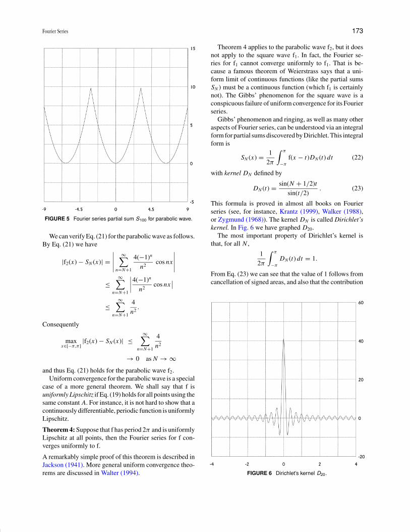
In contrast, the Fourier coefficients of the parabolicwave f2 tend to zero more rapidly (at a rate comparable ton −2). Because of this, the partial sum S100 for f2 is a muchbetter approximation to the parabolic wave (see Fig. 5).In fact, its partial sums SN exhibit the phenomenon ofuniform convergence.

We say that the Fourier series for a function f convergesuniformly to f if

limN →∞

{max

x ∈[−π,π ]|f(x) − SN (x)|

}= 0. (21)

This equation says that, for large enough N , we can havethe maximum distance between the graphs of f and SN assmall as we wish. Figure 5 is a good illustration of this forthe parabolic wave.



Fourier Series 173

FIGURE 5 Fourier series partial sum S100 for parabolic wave.

We can verify Eq. (21) for the parabolic wave as follows.By Eq. (21) we have

|f2(x) − SN (x)| =∣∣∣∣∣

∞∑n =N +1

4(−1)n

n2cos nx

∣∣∣∣∣≤

∞∑n =N +1

∣∣∣∣4(−1)n

n2cos nx

∣∣≤

∞∑n =N +1

4

n2 .

Consequently

maxx ∈[−π,π ]

|f2(x) − SN (x)| ≤∞∑

n =N +1

4

n2

→ 0 as N → ∞and thus Eq. (21) holds for the parabolic wave f2.

Uniform convergence for the parabolic wave is a specialcase of a more general theorem. We shall say that f isuniformly Lipschitz if Eq. (19) holds for all points using thesame constant A. For instance, it is not hard to show that acontinuously differentiable, periodic function is uniformlyLipschitz.

Theorem 4: Suppose that f has period 2π and is uniformlyLipschitz at all points, then the Fourier series for f con-verges uniformly to f.

A remarkably simple proof of this theorem is described inJackson (1941). More general uniform convergence theo-rems are discussed in Walter (1994).

Theorem 4 applies to the parabolic wave f2, but it doesnot apply to the square wave f1. In fact, the Fourier se-ries for f1 cannot converge uniformly to f1. That is be-cause a famous theorem of Weierstrass says that a uni-form limit of continuous functions (like the partial sumsSN ) must be a continuous function (which f1 is certainlynot). The Gibbs’ phenomenon for the square wave is aconspicuous failure of uniform convergence for its Fourierseries.

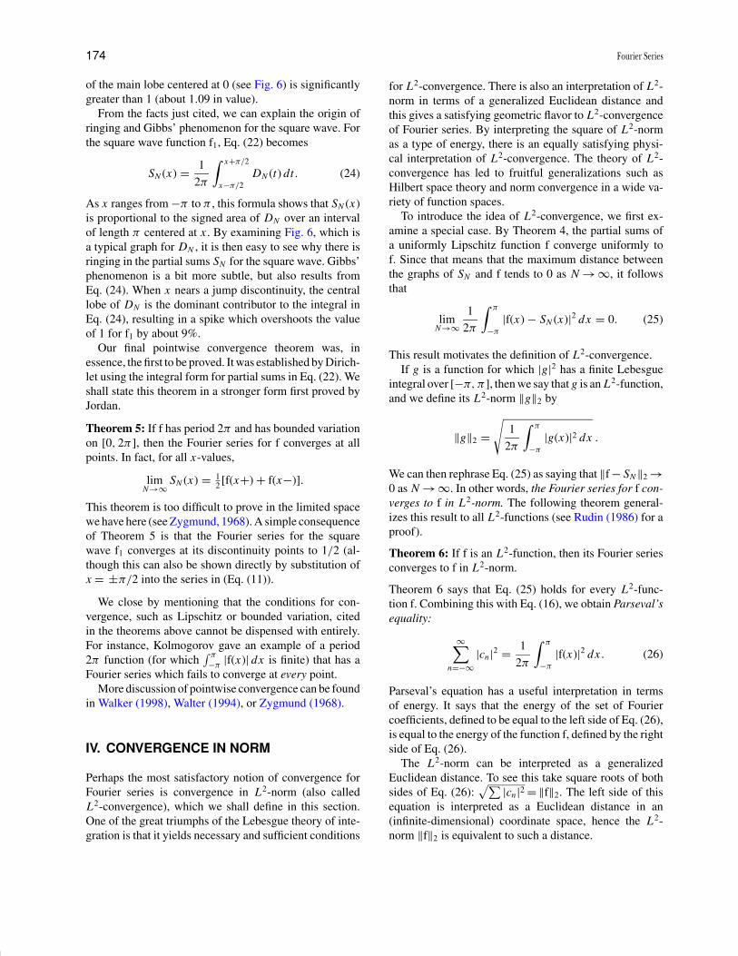
Gibbs’ phenomenon and ringing, as well as many otheraspects of Fourier series, can be understood via an integralform for partial sums discovered by Dirichlet. This integralform is

SN (x) = 1

2π

∫ π

−π

f(x − t)DN (t) dt (22)

with kernel DN defined by

DN (t) = sin(N + 1/2)t

sin(t /2). (23)

This formula is proved in almost all books on Fourierseries (see, for instance, Krantz (1999), Walker (1988),or Zygmund (1968)). The kernel DN is called Dirichlet’skernel. In Fig. 6 we have graphed D20.

The most important property of Dirichlet’s kernel isthat, for all N ,

1

2π

∫ π

−π

DN (t) dt = 1.

From Eq. (23) we can see that the value of 1 follows fromcancellation of signed areas, and also that the contribution

FIGURE 6 Dirichlet’s kernel D20.



174 Fourier Series

of the main lobe centered at 0 (see Fig. 6) is significantlygreater than 1 (about 1.09 in value).

From the facts just cited, we can explain the origin ofringing and Gibbs’ phenomenon for the square wave. Forthe square wave function f1, Eq. (22) becomes

SN (x) = 1

2π

∫ x +π/2

x −π/2DN (t) dt . (24)

As x ranges from −π to π , this formula shows that SN (x)is proportional to the signed area of DN over an intervalof length π centered at x . By examining Fig. 6, which isa typical graph for DN , it is then easy to see why there isringing in the partial sums SN for the square wave. Gibbs’phenomenon is a bit more subtle, but also results fromEq. (24). When x nears a jump discontinuity, the centrallobe of DN is the dominant contributor to the integral inEq. (24), resulting in a spike which overshoots the valueof 1 for f1 by about 9%.

Our final pointwise convergence theorem was, inessence, the first to be proved. It was established by Dirich-let using the integral form for partial sums in Eq. (22). Weshall state this theorem in a stronger form first proved byJordan.

Theorem 5: If f has period 2π and has bounded variationon [0, 2π ], then the Fourier series for f converges at allpoints. In fact, for all x-values,

limN →∞

SN (x) = 12 [f(x +) + f(x −)].

This theorem is too difficult to prove in the limited spacewe have here (see Zygmund, 1968). A simple consequenceof Theorem 5 is that the Fourier series for the squarewave f1 converges at its discontinuity points to 1/2 (al-though this can also be shown directly by substitution ofx = ±π/2 into the series in (Eq. (11)).

We close by mentioning that the conditions for con-vergence, such as Lipschitz or bounded variation, citedin the theorems above cannot be dispensed with entirely.For instance, Kolmogorov gave an example of a period2π function (for which

∫ π

−π|f(x)| dx is finite) that has a

Fourier series which fails to converge at every point.More discussion of pointwise convergence can be found

in Walker (1998), Walter (1994), or Zygmund (1968).

IV. CONVERGENCE IN NORM

Perhaps the most satisfactory notion of convergence forFourier series is convergence in L2-norm (also calledL2-convergence), which we shall define in this section.One of the great triumphs of the Lebesgue theory of inte-gration is that it yields necessary and sufficient conditions

for L2-convergence. There is also an interpretation of L2-norm in terms of a generalized Euclidean distance andthis gives a satisfying geometric flavor to L2-convergenceof Fourier series. By interpreting the square of L2-normas a type of energy, there is an equally satisfying physi-cal interpretation of L2-convergence. The theory of L2-convergence has led to fruitful generalizations such asHilbert space theory and norm convergence in a wide va-riety of function spaces.

To introduce the idea of L2-convergence, we first ex-amine a special case. By Theorem 4, the partial sums ofa uniformly Lipschitz function f converge uniformly tof. Since that means that the maximum distance betweenthe graphs of SN and f tends to 0 as N → ∞, it followsthat

limN →∞

1

2π

∫ π

−π

|f(x) − SN (x)|2 dx = 0. (25)

This result motivates the definition of L2-convergence.If g is a function for which |g |2 has a finite Lebesgue

integral over [−π, π], then we say that g is an L2-function,and we define its L2-norm ‖g ‖2 by

‖g ‖2 =√

1

2π

∫ π

−π

|g(x)|2 dx .

We can then rephrase Eq. (25) as saying that ‖f − SN ‖2 →0 as N → ∞. In other words, the Fourier series for f con-verges to f in L2-norm. The following theorem general-izes this result to all L2-functions (see Rudin (1986) for aproof).

Theorem 6: If f is an L2-function, then its Fourier seriesconverges to f in L2-norm.

Theorem 6 says that Eq. (25) holds for every L2-func-tion f. Combining this with Eq. (16), we obtain Parseval’sequality:

∞∑n=−∞

|cn|2 = 1

2π

∫ π

−π

|f(x)|2 dx . (26)

Parseval’s equation has a useful interpretation in termsof energy. It says that the energy of the set of Fouriercoefficients, defined to be equal to the left side of Eq. (26),is equal to the energy of the function f, defined by the rightside of Eq. (26).

The L2-norm can be interpreted as a generalizedEuclidean distance. To see this take square roots of bothsides of Eq. (26):

√∑ |cn |2 = ‖f‖2. The left side of thisequation is interpreted as a Euclidean distance in an(infinite-dimensional) coordinate space, hence the L2-norm ‖f‖2 is equivalent to such a distance.



Fourier Series 175

As examples of these ideas, let’s return to the squarewave and parabolic wave. For the square wave f1, we findthat

‖f1 − S100 ‖22 =

∑|n |>100

sin2(n π/2)

(n π )2

= 1.0 × 10−3 .

Likewise, for the parabolic wave f2, we have ‖f2 −S100 ‖2

2 = 2.6 × 10−6. These facts show that the energyof the parabolic wave is almost entirely contained inthe partial sum S100; their energy difference is almostthree orders of magnitude smaller than in the square wavecase. In terms of generalized Euclidean distance, we have‖f2 − S100 ‖2 = 1.6 × 10−3 and ‖f1 − S100 ‖2 = 3.2 × 10−2,showing that the partial sum is an order of magnitudecloser for the parabolic wave.

Theorem 6 has a converse, known as the Riesz-Fischertheorem.

Theorem 7 (Riesz-Fischer): If∑ |cn |2 converges, then

there exists an L2-function f having {cn } as its Fouriercoefficients.

This theorem is proved in Rudin (1986). Theorem andthe Riesz-Fischer theorem combine to give necessary andsufficient conditions for L2-convergence of Fourier series,conditions which are remarkably easy to apply. This hasmade L2-convergence into the most commonly used no-tion of convergence for Fourier series.

These ideas for L2-norms partially generalize to thecase of L p-norms. Let p be real number satisfying p ≥ 1.If g is a function for which |g |p has a finite Lebesgueintegral over [−π, π ], then we say that g is an L p-function,and we define its L p-norm ‖g ‖p by

‖g ‖p =[

1

2π

∫ π

−π

|g(x)|p dx

]1/p

.

If ‖f − SN ‖p → 0, then we say that the Fourier series forf converges to f in L p-norm. The following theorem gen-eralizes Theorem 6 (see Krantz (1999) for a proof).

Theorem 8: If f is an L p-function for p > 1, then itsFourier series converges to f in L p-norm.

Notice that the case of p = 1 is not included in Theorem 8.The example of Kolmogorov cited at the end of Section IIIshows that there exist L1-functions whose Fourier seriesdo not converge in L1-norm. For p �= 2, there are no simpleanalogs of either Parseval’s equality or the Riesz-Fischertheorem (which say that we can characterize L2-functionsby the magnitude of their Fourier coefficients). Some par-tial analogs of these latter results for L p-functions, whenp �= 2, are discussed in Zygmund (1968) (in the context ofLittlewood-Paley theory).

We close this section by returning full circle to the no-tion of pointwise convergence. The following theorem wasproved by Carleson for L2-functions and by Hunt for L p-functions (p �= 2).

Theorem 9: If f is an L p-function for p > 1, then itsFourier series converges to it at almost all points.

By almost all points, we mean that the set of points wheredivergence occurs has Lebesgue measure zero. Referencesfor the proof of Theorem 9 can be found in Krantz (1999)and Zygmund (1968). Its proof is undoubtedly the mostdifficult one in the theory of Fourier series.

V. SUMMABILITY OF FOURIER SERIES

In the previous sections, we noted some problems withconvergence of Fourier series partial sums. Some of theseproblems include Kolmogorov’s example of a Fourierseries for an L1-function that diverges everywhere, andGibbs’ phenomenon and ringing in the Fourier series par-tial sums for discontinuous functions. Another problemis Du Bois Reymond’s example of a continuous functionwhose Fourier series diverges on a countably infinite set ofpoints, see Walker (1968). It turns out that all of these dif-ficulties simply disappear when new summation methods,based on appropriate modifications of the partial sums, areused.

The simplest modification of partial sums, and one ofthe first historically to be used, is to take arithmeticmeans. Define the N th arithmetic mean σN by σN =(S0 + S1 + · · · + SN−1)/N . From which it follows that

σN (x) =N∑

n=−N

(1 − |n|

N

)cn einx . (27)

The factors (1 − |n|/N ) are called convergence factors.They modify the Fourier coefficients cn so that the am-plitude of the higher frequency terms (for |n| near N ) aredamped down toward zero. This produces a great improve-ment in convergence properties as shown by the followingtheorem.

Theorem 10: Let f be a periodic function. If f is an L p-function for p ≥ 1, then σN → f in L p-norm as N → ∞.If f is a continuous function, then σN → f uniformly asN → ∞.

Notice that L1-convergence is included in Theorem 10.Even for Kolmogorov’s function, it is the case that‖f − σN ‖1 → 0 as N → ∞. It also should be noted thatno assumption, other than continuity of the periodic func-tion, is needed in order to ensure uniform convergence ofits arithmetic means.



176 Fourier Series

For a proof of Theorem 10, see Krantz (1999). The keyto the proof is Fejer’s integral form for σN :

σN (x) = 1

2π

∫ π

−π

f(x − t)FN (t) dt (28)

where Fejer’s kernel FN is defined by

FN (t) = 1

N

(sin Nt/2

sin t /2

)2

. (29)

In Fig. 7 we show the graph of F20. Compare this graphwith the one of Dirichlet’s kernel D20 in Fig. 6. UnlikeDirichlet’s kernel, Fejer’s kernel is positive [FN (t) ≥ 0],and is close to 0 away from the origin. These two factsare the main reasons that Theorem 10 holds. The fact thatFejer’s kernel satisfies

1

2π

∫ π

−π

FN (t) dt = 1

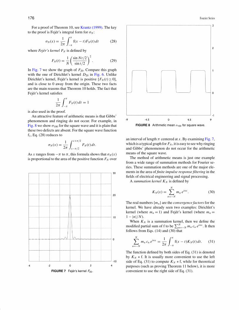
is also used in the proof.An attractive feature of arithmetic means is that Gibbs’

phenomenon and ringing do not occur. For example, inFig. 8 we show σ100 for the square wave and it is plain thatthese two defects are absent. For the square wave functionf1, Eq. (28) reduces to

σN (x) = 1

2π

∫ x +π/2

x −π/2FN (t) dt .

As x ranges from −π to π , this formula shows that σN (x)is proportional to the area of the positive function FN over

FIGURE 7 Fejer’s kernel F20.

FIGURE 8 Arithmetic mean σ100 for square wave.

an interval of length π centered at x . By examining Fig. 7,which is a typical graph for FN , it is easy to see why ringingand Gibbs’ phenomenon do not occur for the arithmeticmeans of the square wave.

The method of arithmetic means is just one examplefrom a wide range of summation methods for Fourier se-ries. These summation methods are one of the major ele-ments in the area of finite impulse response filtering in thefields of electrical engineering and signal processing.

A summation kernel KN is defined by

KN (x) =N∑

n=−N

mn einx . (30)

The real numbers {mn} are the convergence factors for thekernel. We have already seen two examples: Dirichlet’skernel (where mn = 1) and Fejer’s kernel (where mn =1 − |n|/N ).

When KN is a summation kernel, then we define themodified partial sum of f to be

∑Nn=−N mn cn einx . It then

follows from Eqs. (14) and (30) that

N∑n=−N

mn cn einx = 1

2π

∫ π

−π

f(x − t)KN (t) dt. (31)

The function defined by both sides of Eq. (31) is denotedby KN ∗ f. It is usually more convenient to use the leftside of Eq. (31) to compute KN ∗ f, while for theoreticalpurposes (such as proving Theorem 11 below), it is moreconvenient to use the right side of Eq. (31).



Fourier Series 177

We say that a summation kernel KN is regular if itsatisfies the following three conditions.

1. For each N ,

1

2π

∫ π

−π

KN (x) dx = 1.

2. There is a positive constant C such that

1

2π

∫ π

−π

|KN (x)| dx ≤ C .

3. For each 0 < δ < π ,

limN →∞

{max

δ≤|x |≤π|KN (x)|

}= 0.

There are many examples of regular summation kernels.Fejer’s kernel, which has mn = 1 − |n |/N , is regular. An-other regular summation kernel is Hann’s kernel, whichhas mn = 0.5 + 0.5 cos(n π/N ). A third regular summa-tion kernel is de le Vallee Poussin’s kernel, for whichmn = 1 when |n | ≤ N /2, and mn = 2(1 − |m /N |) whenN /2 < |m | ≤ N . The proofs that these summation kernelsare regular are given in Walker (1996). It should be notedthat Dirichlet’s kernel is not regular, because properties 2and 3 do not hold.

As with Fejer’s kernel, all regular summation kernelssignificantly improve the convergence of Fourier series.In fact, the following theorem generalizes Theorem 10.

Theorem 11: Let f be a periodic function, and let KN be aregular summation kernel. If f is an L p-function for p ≥ 1,then KN ∗f → f in L p-norm as N → ∞. If f is a continuousfunction, then KN ∗ f → f uniformly as N → ∞.

For an elegant proof of this theorem, see Krantz (1999).From Theorem 11 we might be tempted to conclude

that the convergence properties of regular summation ker-nels are all the same. They do differ, however, in the ratesat which they converge. For example, in Fig. 9 we showK100 ∗ f1 where the kernel is Hann’s kernel and f1 is thesquare wave. Notice that this graph is a much better ap-proximation of a square wave than the arithmetic meangraph in Fig. 8. An oscilloscope, for example, can easilygenerate the graph in Fig. 9, thereby producing an accept-able version of a square wave.

Summation of Fourier series is discussed furtherin Krantz (1999), Walker (1996), Walter (1994), andZygmund (1968).

VI. GENERALIZED FOURIER SERIES

The classical theory of Fourier series has undergone ex-tensive generalizations during the last two hundred years.

FIGURE 9 Approximate square wave using Hann’s kernel.

For example, Fourier series can be viewed as one aspectof a general theory of orthogonal series expansions. Inthis section, we shall discuss a few of the more celebratedorthogonal series, such as Legendre series, Haar series,and wavelet series.

We begin with Legendre series. The first two Legendrepolynomials are P0(x) = 1, and P1(x) = x . For n = 2,

3, 4, . . . , the nth Legendre polynomial Pn is defined bythe recursion relation

n Pn(x) = (2n − 1)x Pn−1(x) + (n − 1)Pn−2(x).

These polynomials satisfy the following orthogonalityrelation∫ 1

−1Pn(x) Pm(x) dx =

{0 if m �= n

(2n + 1)/2 if m = n.(32)

This equation is quite similar to Eq. (14). Because ofEq. (32)—recall how we used Eq. (14) to derive Eq. (9)—the Legendre series for a function f over the interval[−1, 1] is defined to be

∞∑n=0

cn Pn(x) (33)

with

cn = 2

2n + 1

∫ 1

−1f(x) Pn(x) dx . (34)



178 Fourier Series

FIGURE 10 Step function and its Legendre series partial sumS11.

The partial sum SN of the series in Eq. (33) is defined tobe

SN (x) =N∑

n =0

cn Pn(x).

As an example, let f(x) = 1 for 0 ≤ x ≤ 1 and f(x) = 0for −1 ≤ x < 0. The Legendre series for this step functionis [see Walker (1988)]:

1

2+

∞∑k =0

(−1)k(4k + 3)(2k)!

4k +1(k + 1)!k!P2k +1(x).

In Fig. 10 we show the partial sum S11 for this series. Thegraph of S11 is reminiscent of a Fourier series partial sumfor a step function. In fact, the following theorem is true.

Theorem 12: If∫ 1−1 |f(x)|2 dx is finite, then the partial

sums SN for the Legendre series for f satisfy

limN →∞

∫ 1

−1|f(x) − SN (x)|2 dx = 0.

Moreover, if f is Lipschitz at a point x0, then SN (x0) →f(x0) as N → ∞.

This theorem is proved in Walter (1994) and Jackson(1941). Further details and other examples of orthogonalpolynomial series can be found in either Davis (1975),Jackson (1941), or Walter (1994). There are many impor-tant orthogonal series—such as Hermite, Laguerre, and

Tchebysheff—which we cannot examine here because ofspace limitations.

We now turn to another type of orthogonal series, theHaar series. The defects, such as Gibbs’ phenomenon andringing, that occur with Fourier series expansions can betraced to the unlocalized nature of the functions used forexpansions. The complex exponentials used in classicalFourier series, and the polynomials used in Legendre se-ries, are all non-zero (except possibly for a finite number ofpoints) over their domains. In contrast, Haar series makeuse of localized functions, which are non-zero only overtiny regions within their domains.

In order to define Haar series, we first define the funda-mental Haar wavelet H (x) by

H (x) ={

1 if 0 ≤ x < 1/2

−1 if 1/2 ≤ x ≤ 1.

The Haar wavelets {Hj ,k(x)} are then defined by

Hj ,k(x) = 2 j /2 H (2 j x − k)

for j = 0, 1, 2, . . . ; k = 0, 1, . . . , 2 j − 1. Notice thatHj ,k(x) is non-zero only on the interval [k2− j ,

(k + 1)2− j ], which for large j is a tiny subinterval of [0, 1].As k ranges between 0 and 2 j − 1, these subintervals par-tition the interval [0, 1], and the partition becomes finer(shorter subintervals) with increasing j .

The Haar series for a function f is defined by

b +∞∑j =0

2 j −1∑k =0

c j ,k Hj ,k(x) (35)

with b = ∫ 10 f(x) dx and

c j ,k =∫ 1

0f (x) Hj ,k(x) dx .

The definitions of b and c j ,k are justified by orthogonalityrelations between the Haar functions (similar to the or-thogonality relations that we used above to justify Fourierseries and Legendre series).

A partial sum SN for the Haar series in Eq. () is definedby

SN (x) = b +∑

{ j,k | 2 j +k≤N }c j,k Hj,k(x).

For example, let f be the function on [0, 1] defined asfollows

f(x) ={

x − 1/2 if 1/4 < x < 3/4

0 if x ≤ 1/4 or 3/4 ≤ x .

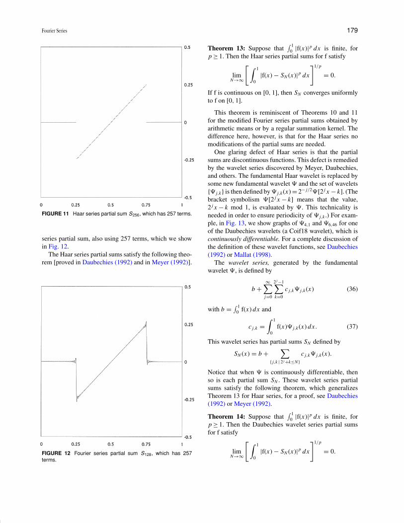
In Fig. 11 we show the Haar series partial sum S256 for thisfunction. Notice that there is no Gibbs’ phenomenon withthis partial sum. This contrasts sharply with the Fourier



Fourier Series 179

FIGURE 11 Haar series partial sum S256, which has 257 terms.

series partial sum, also using 257 terms, which we showin Fig. 12.

The Haar series partial sums satisfy the following theo-rem [proved in Daubechies (1992) and in Meyer (1992)].

FIGURE 12 Fourier series partial sum S128, which has 257terms.

Theorem 13: Suppose that∫ 1

0 |f(x)|p dx is finite, forp ≥ 1. Then the Haar series partial sums for f satisfy

limN →∞

[ ∫ 1

0|f(x) − SN (x)|p dx

]1/p

= 0.

If f is continuous on [0, 1], then SN converges uniformlyto f on [0, 1].

This theorem is reminiscent of Theorems 10 and 11for the modified Fourier series partial sums obtained byarithmetic means or by a regular summation kernel. Thedifference here, however, is that for the Haar series nomodifications of the partial sums are needed.

One glaring defect of Haar series is that the partialsums are discontinuous functions. This defect is remediedby the wavelet series discovered by Meyer, Daubechies,and others. The fundamental Haar wavelet is replaced bysome new fundamental wavelet and the set of wavelets{ j ,k } is then defined by j ,k(x) = 2− j /2 [2 j x − k]. (Thebracket symbolism [2 j x − k] means that the value,2 j x − k mod 1, is evaluated by . This technicality isneeded in order to ensure periodicity of j ,k .) For exam-ple, in Fig. 13, we show graphs of 4,1 and 6,46 for oneof the Daubechies wavelets (a Coif18 wavelet), which iscontinuously differentiable. For a complete discussion ofthe definition of these wavelet functions, see Daubechies(1992) or Mallat (1998).

The wavelet series, generated by the fundamentalwavelet , is defined by

b +∞∑j =0

2 j −1∑k =0

c j ,k j ,k(x) (36)

with b = ∫ 10 f(x) dx and

c j ,k =∫ 1

0f(x) j ,k(x) dx . (37)

This wavelet series has partial sums SN defined by

SN (x) = b +∑

{ j ,k | 2 j +k ≤N }c j ,k j ,k(x).

Notice that when is continuously differentiable, thenso is each partial sum SN . These wavelet series partialsums satisfy the following theorem, which generalizesTheorem 13 for Haar series, for a proof, see Daubechies(1992) or Meyer (1992).


0 |f(x)|p dx is finite, forp ≥ 1. Then the Daubechies wavelet series partial sumsfor f satisfy

limN→∞

[ ∫ 1


]1/p

= 0.



180 Fourier Series

FIGURE 13 Two Daubechies wavelets.

If f is continuous on [0, 1], then SN converges uniformlyto f on [0, 1].

Theorem 14 does not reveal the full power of waveletseries. In almost all cases, it is possible to rearrange theterms in the wavelet series in any manner whatsoever andconvergence will still hold. One reason for doing a rear-rangement is in order to add the terms in the series withcoefficients of largest magnitude (thus largest energy) firstso as to speed up convergence to the function. Here is aconvergence theorem for such permuted series.


0 |f(x)|p dx is finite, forp > 1. If the terms of a Daubechies wavelet series are per-muted (in any manner whatsoever), then the partial sumsSN of the permuted series satisfy

limN →∞

[ ∫ 1


]1/p

= 0.

If f is uniformly Lipschitz, then the partial sums SN of thepermuted series converge uniformly to f.

This theorem is proved in Daubechies (1992) and Meyer(1992). This type of convergence of wavelet series iscalled unconditional convergence. It is known [see Mallat(1998)] that unconditional convergence of wavelet seriesensures an optimality of compression of signals. For de-tails about compression of signals and other applicationsof wavelet series, see Walker (1999) for a simple intro-duction and Mallat (1998) for a thorough treatment.

VII. DISCRETE FOURIER SERIES

The digital computer has revolutionized the practice ofscience in the latter half of the twentieth century. Themethods of computerized Fourier series, based upon thefast Fourier transform algorithms for digital approxima-tion of Fourier series, have completely transformed theapplication of Fourier series to scientific problems. In thissection, we shall briefly outline the main facts in the theoryof discrete Fourier series.

The Fourier series coefficients {cn } can be discretely ap-proximated via Riemann sums for the integrals in Eq. (9).For a (large) positive integer M , let xk = −π + 2πk /Mfor k = 0, 1, 2, . . . , M − 1 and let �x = 2π/M . Then thenth Fourier coefficient cn for a function f is approximatedas follows:

cn ≈ 1

2π

M −1∑k =0

f(xk) e −i2πnxk�x

= e −inπ

M

M −1∑k =0

f(xk)e −i2πkn/M .

The last sum above is called the Discrete Fourier Trans-form (DFT) of the finite sequence of numbers {f(xk)}.That is, we define the DFT of a sequence {gk}M−1

k=0 ofnumbers by

Gn =M−1∑k=0

gk e−i2πkn/M . (38)

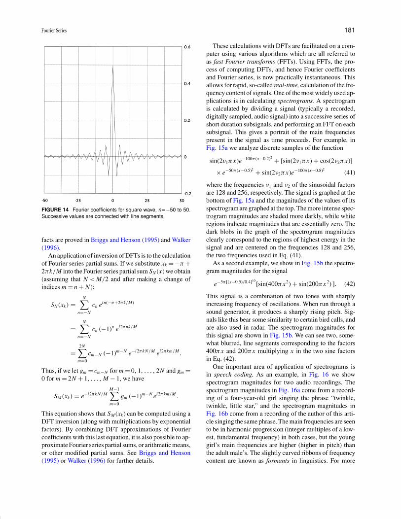
The DFT is the set of numbers {Gn}, and we see from thediscussion above that the Fourier coefficients of a functionf can be approximated by a DFT (multiplied by the fac-tors e −inπ/M). For example, in Fig. 14 we show a graphof approximations of the Fourier coefficients {cn}50

n=−50 ofthe square wave f1 obtained via a DFT (using M = 1024).For all values, these approximate Fourier coefficients dif-fer from the exact coefficients by no more than 10−3. Bytaking M even larger, the error can be reduced still further.

The two principal properties of DFTs are that they canbe inverted and they preserve energy (up to a scale factor).The inversion formula for the DFT is

gk =M−1∑n=0

Gn ei2πkn/M . (39)

And the conservation of energy property is

M−1∑k=0

|gk |2 = 1

N

M−1∑n=0

|Gn|2. (40)

Interpreting a sum of squares as energy, Eq. (40) says that,up to multiplication by the factor 1/N , the energy of thediscrete signal {gk} and its DFT {Gn} are the same. These



Fourier Series 181

FIGURE 14 Fourier coefficients for square wave, n = −50 to 50.Successive values are connected with line segments.

facts are proved in Briggs and Henson (1995) and Walker(1996).

An application of inversion of DFTs is to the calculationof Fourier series partial sums. If we substitute xk = −π +2πk /M into the Fourier series partial sum SN (x) we obtain(assuming that N < M /2 and after making a change ofindices m = n + N ):

SN (xk) =N∑

n =−N

cn ein(−π+2πk /M)

=N∑

n =−N

cn (−1)n ei2πnk /M

=2N∑

m =0

cm −N (−1)m −N e −i2πk N/M ei2πkm/M .

Thus, if we let gm = cm −N for m = 0, 1, . . . , 2N and gm =0 for m = 2N + 1, . . . , M − 1, we have

SM (xk) = e −i2πk N/MM −1∑m =0

gm (−1)m −N ei2πkm/M .

This equation shows that SM (xk) can be computed using aDFT inversion (along with multiplications by exponentialfactors). By combining DFT approximations of Fouriercoefficients with this last equation, it is also possible to ap-proximate Fourier series partial sums, or arithmetic means,or other modified partial sums. See Briggs and Henson(1995) or Walker (1996) for further details.

These calculations with DFTs are facilitated on a com-puter using various algorithms which are all referred toas fast Fourier transforms (FFTs). Using FFTs, the pro-cess of computing DFTs, and hence Fourier coefficientsand Fourier series, is now practically instantaneous. Thisallows for rapid, so-called real-time, calculation of the fre-quency content of signals. One of the most widely used ap-plications is in calculating spectrograms. A spectrogramis calculated by dividing a signal (typically a recorded,digitally sampled, audio signal) into a successive series ofshort duration subsignals, and performing an FFT on eachsubsignal. This gives a portrait of the main frequenciespresent in the signal as time proceeds. For example, inFig. 15a we analyze discrete samples of the function

sin(2ν1 πx)e −100π (x −0.2)2 + [sin(2ν1 πx) + cos(2ν2 πx)]

× e −50π (x −0.5)2 + sin(2ν2 πx)e −100π (x −0.8)2(41)

where the frequencies ν1 and ν2 of the sinusoidal factorsare 128 and 256, respectively. The signal is graphed at thebottom of Fig. 15a and the magnitudes of the values of itsspectrogram are graphed at the top. The more intense spec-trogram magnitudes are shaded more darkly, while whiteregions indicate magnitudes that are essentially zero. Thedark blobs in the graph of the spectrogram magnitudesclearly correspond to the regions of highest energy in thesignal and are centered on the frequencies 128 and 256,the two frequencies used in Eq. (41).

As a second example, we show in Fig. 15b the spectro-gram magnitudes for the signal

e −5π [(x −0.5)/0.4]10 [sin(400πx2) + sin(200πx2) ]. (42)

This signal is a combination of two tones with sharplyincreasing frequency of oscillations. When run through asound generator, it produces a sharply rising pitch. Sig-nals like this bear some similarity to certain bird calls, andare also used in radar. The spectrogram magnitudes forthis signal are shown in Fig. 15b. We can see two, some-what blurred, line segments corresponding to the factors400πx and 200πx multiplying x in the two sine factorsin Eq. (42).

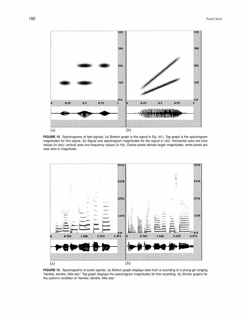
One important area of application of spectrograms isin speech coding. As an example, in Fig. 16 we showspectrogram magnitudes for two audio recordings. Thespectrogram magnitudes in Fig. 16a come from a record-ing of a four-year-old girl singing the phrase “twinkle,twinkle, little star,” and the spectrogram magnitudes inFig. 16b come from a recording of the author of this arti-cle singing the same phrase. The main frequencies are seento be in harmonic progression (integer multiples of a low-est, fundamental frequency) in both cases, but the younggirl’s main frequencies are higher (higher in pitch) thanthe adult male’s. The slightly curved ribbons of frequencycontent are known as formants in linguistics. For more



182 Fourier Series

FIGURE 15 Spectrograms of test signals. (a) Bottom graph is the signal in Eq. (41). Top graph is the spectrogrammagnitudes for this signal. (b) Signal and spectrogram magnitudes for the signal in (42). Horizontal axes are timevalues (in sec); vertical axes are frequency values (in Hz). Darker pixels denote larger magnitudes, white pixels arenear zero in magnitude.

FIGURE 16 Spectrograms of audio signals. (a) Bottom graph displays data from a recording of a young girl singing“twinkle, twinkle, little star.” Top graph displays the spectrogram magnitudes for this recording. (b) Similar graphs forthe author’s rendition of “twinkle, twinkle, little star.”



Fourier Series 183

details on the use of spectrograms in signal analysis, seeMallat (1998).

It is possible to invert spectrograms. In other words, wecan recover the original signal by inverting the successionof DFTs that make up its spectrogram. One applicationof this inverse procedure is to the compression of audiosignals. After discarding (setting to zero) all the values inthe spectrogram with magnitudes below a threshold value,the inverse procedure creates an approximation to the sig-nal which uses significantly less data than the originalsignal. For example, by discarding all of the spectrogramvalues having magnitudes less than 1/320 times the largestmagnitude spectrogram value, the young girl’s version of“twinkle, twinkle, little star” can be approximated, withoutnoticeable degradation of quality, using about one-eighththe amount of data as the original recording. Some of thebest results in audio compression are based on sophis-ticated generalizations of this spectrogram technique—referred to either as lapped transforms or as local cosineexpansions, see Malvar (1992) and Mallat (1998).

VIII. CONCLUSION

In this article, we have outlined the main features ofthe theory and application of one-variable Fourier series.Much additional information, however, can be found inthe references. In particular, we did not have sufficientspace to discuss the intricacies of multivariable Fourierseries which, for example, have important applicationsin crystallography and molecular structure determination.For a mathematical introduction to multivariable Fourierseries, see Krantz (1999), and for an introduction to theirapplications, see Walker (1988).

SEE ALSO THE FOLLOWING ARTICLES

FUNCTIONAL ANALYSIS • GENERALIZED FUNCTIONS •MEASURE AND INTEGRATION • NUMERICAL ANALYSIS •SIGNAL PROCESSING • WAVELETS

BIBLIOGRAPHY

Briggs, W. L., and Henson, V. E. (1995). “The DFT. An Owner’s Manual,”SIAM, Philadelphia.

Daubechies, I. (1992). “Ten Lectures on Wavelets,” SIAM, Philadelphia.Davis, P. J. (1975). “Interpolation and Approximation,” Dover, New

York.Davis, P. J., and Hersh, R. (1982). “The Mathematical Experience,”

Houghton Mifflin, Boston.Fourier, J. (1955). “The Analytical Theory of Heat,” Dover, New York.Jackson, D. (1941). “Fourier Series and Orthogonal Polynomials,” Math.

Assoc. of America, Washington, DC.Krantz, S. G. (1999). “A Panorama of Harmonic Analysis,” Math. Assoc.

of America, Washington, DC.Mallat, S. (1998). “A Wavelet Tour of Signal Processing,” Academic

Press, New York.Malvar, H. S. (1992). “Signal Processing with Lapped Transforms,”

Artech House, Norwood.Meyer, Y. (1992). “Wavelets and Operators,” Cambridge Univ. Press,

Cambridge.Rudin, W. (1986). “Real and Complex Analysis,” 3rd edition, McGraw-

Hill, New York.Walker, J. S. (1988). “Fourier Analysis,” Oxford Univ. Press, Oxford.Walker, J. S. (1996). “Fast Fourier Transforms,” 2nd edition, CRC Press,

Boca Raton.Walker, J. S. (1999). “A Primer on Wavelets and their Scientific Appli-

cations,” CRC Press, Boca Raton.Walter, G. G. (1994). “Wavelets and Other Orthogonal Systems with

Applications,” CRC Press, Boca Raton.Zygmund, A. (1968). “Trigonometric Series,” Cambridge Univ. Press,

Cambridge.

Qu: 00, 00, 00, 00 - Apache2 Ubuntu Default Page: It works GHA/LOW P2: FQP Final Qu: 00, 00, 00, 00...

Documents

Transcript of Qu: 00, 00, 00, 00 - Apache2 Ubuntu Default Page: It works GHA/LOW P2: FQP Final Qu: 00, 00, 00, 00...