
QTLNetwork-2.0 User Manual
30
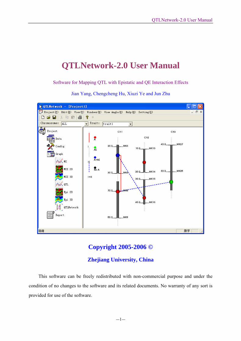
QTLNetwork-2.0 User Manual ―1― QTLNetwork-2.0 User Manual Software for Mapping QTL with Epistatic and QE Interaction Effects Jian Yang, Chengcheng Hu, Xiuzi Ye and Jun Zhu Copyright 2005-2006 © Zhejiang University, China This software can be freely redistributed with non-commercial purpose and under the condition of no changes to the software and its related documents. No warranty of any sort is provided for use of the software.
Transcript of QTLNetwork-2.0 User Manual
QTLNetwork-2.0 User Manual
―1―
QTLNetwork-2.0 User Manual
Software for Mapping QTL with Epistatic and QE Interaction Effects
Jian Yang, Chengcheng Hu, Xiuzi Ye and Jun Zhu
Copyright 2005-2006 ©
Zhejiang University, China
This software can be freely redistributed with non-commercial purpose and under the
condition of no changes to the software and its related documents. No warranty of any sort is
provided for use of the software.
QTLNetwork-2.0 User Manual
―2―
Contents
QTLNetwork-2.0 User Guide ............................................................ 1
1. Introduction to QTLNetwork ................................................... 3
2. Installing QTLNetwork............................................................ 3
3. Running QTLNetwork ............................................................. 6
4. Starting with QTLNetwork ...................................................... 7
4.1. Data Format..................................................................... 7
4.2. Create new project with map and data files. ................. 13
4.3. Open the project with map, data and result files........... 21
5. Interactive Visualization operations....................................... 22
6. Config setting in the mapping computation........................... 23
6.1. General page.................................................................. 24
6.2. Genome scan configuration page.................................. 25
6.3. Significance level configuration page........................... 25
6.4. Output configuration page............................................. 26
7. Graph setting .......................................................................... 26
8. Save pictures and reports ....................................................... 27
8.1. Save pictures. ................................................................ 27
8.2. Save and understand the text reports............................. 27
QTLNetwork-2.0 User Manual
―3―
1. Introduction to QTLNetwork
QTLNetwork-2.0 is user-friendly computer software for mapping quantitative trait loci
(QTL) with epistatic effects and QTL by environment (QE) interaction effects in DH, RI,
BC1, BC2, F2, IF2 and BxFy populations, and for graphical presentation of QTL mapping
results. The software is developed based on the MCIM (mixed-model based composite
interval mapping) method, and programmed by C++ programming language under Microsoft
Visual C++ 6.0 environment. The GUI (Graphic User Interface) of QTLNetwork is developed
by MFC (Microsoft Foundation Class) and the graphic visualization is done by VTK
(Visualization Tookit). This software works with Microsoft Windows operating systems,
including Windows 95/98, NT, 2000, XP, 2003server. A new version of QTLNetwork is
under developing, and its functions will be extended to include marker-assisted virtual
breeding. Considering that most users are using Microsoft Windows system, we will only
describe the application of GUI version of QTLNetwork in the following section.
2 Installing QTLNetwork The software is freely available from the URL http://ibi.zju.edu.cn/software/qtlnetwork/.
Download the QTLNetwork setup package QTLNetwork-2.0-Setup.exe , and double
click it. The setup welcome screen displays as following.
Click the button of next, and
enter to the screen of License
agreement.
QTLNetwork-2.0 User Manual
―4―
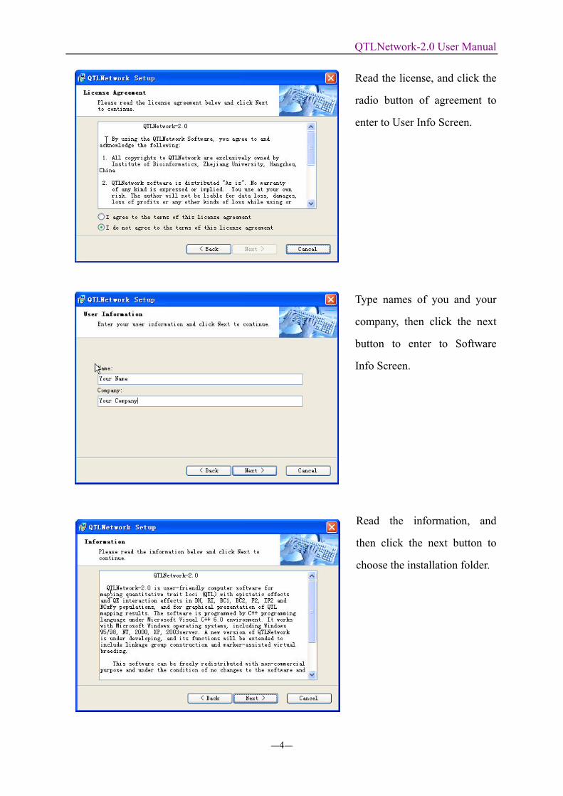
Read the license, and click the
radio button of agreement to
enter to User Info Screen.
Type names of you and your
company, then click the next
button to enter to Software
Info Screen.
Read the information, and
then click the next button to
choose the installation folder.
QTLNetwork-2.0 User Manual
―5―
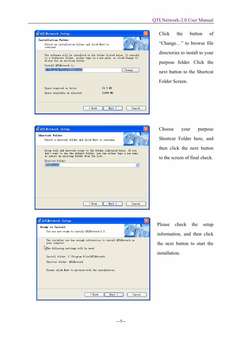
Click the button of
“Change…” to browse file
directories to install to your
purpose folder. Click the
next button to the Shortcut
Folder Screen.
Choose your purpose
Shortcut Folder here, and
then click the next button
to the screen of final check.
Please check the setup
information, and then click
the next button to start the
installation.
QTLNetwork-2.0 User Manual
―6―
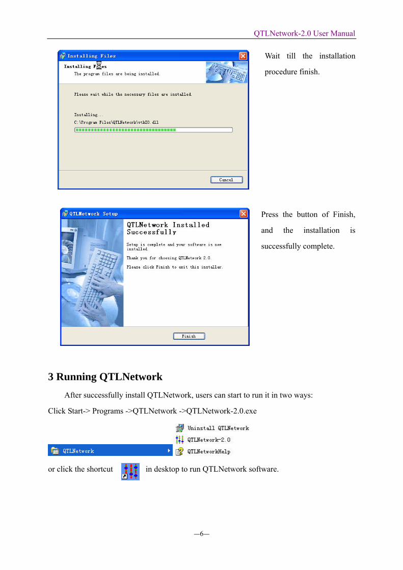
Wait till the installation
procedure finish.
Press the button of Finish,
and the installation is
successfully complete.
3 Running QTLNetwork After successfully install QTLNetwork, users can start to run it in two ways:
Click Start-> Programs ->QTLNetwork ->QTLNetwork-2.0.exe
or click the shortcut in desktop to run QTLNetwork software.
QTLNetwork-2.0 User Manual
―7―
4 Starting with QTLNetwork
4.1 Data Format
For performing analyses with QTLNetwork 2.0, two source data files are required: a
marker linkage map file (for simplification, we call it map file) and a data file. A map file
contains information about the order and genetic distances of all observed markers on the
chromosomes or linkage groups. A data file contains observations of the markers and the
traits under study for all individuals. We provide some sample files for briefly demonstrating
the format of source data files for QTLNetwork 2.0 in the sub-directory (\SampleData) where
QTLNetwork has been installed. The map and data files for QTLMapper software can be
directly used by QTLNetwork 2.0.
4.1.1 Format of marker linkage map file
This file contains information about the marker linkage map, such as the number of
chromosomes, number and order of markers on each of the chromosomes, flanking marker
distances, etc. It consists of general description and map body. General Description: This part is in the front of map file. A typical general description looks
like:
_DistanceUnit cM
_MapFunction K
_Chromosomes 4
_MarkerNumbers 6 4 7 9
There are a total of four possible items for general description. They can be in any order.
Each item in general description is a key word followed by certain specification(s). Each key
string must be started with an underline “_”, and there should not be any list separator (white
space or table) within the key string. The specification(s) must be separated from the key
word by at least one list separator, and there must also be at least one list separator between
any two neighboring specifications if two or more specifications are included for the item. A
key string and its specification(s) must be placed in the same line. Both key strings and
specification(s) (if characters) are not case insensitive. _DistanceUnit specifies the unit of genetic distances used in the map file. The specification
string “cM” stands for centi-Morgan and “M” stands for Morgan.
QTLNetwork-2.0 User Manual
―8―
_MapFunction indicates the map function used in creating the marker linkage map for
transforming recombination fractions into genetic distances. Specification character “K” is for
Kosambi function and “H” for Haldane function.
_Chromosomes is for specifying the total number of chromosomes or linkage groups
involved in the map file.
_MarkerNumbers is for specifying the number of markers on each of the chromosomes. The
order of the numbers must be consistent with that for genetic-distance columns in the map
body.
Map Body: This part starts from key string *MapBegin* and ends at key string *MapEnd*. A
typical map body looks like:
*MapBegin*
Marker# Ch1 Ch2 Ch3 Ch4
1 0.00 0.00 0.00 0.00
2 9.84 11.26 7.45 9.85
3 10.22 8.69 9.10 10.93
4 8.25 9.87 10.66 10.70
5 9.79 10.16 10.10
6 7.47 8.34 11.30
7 11.21 9.30
8 7.23
9 11.78
*MapEnd*
The strings (Marker#, Ch1, Ch2, Ch3, Ch4) in the second row show the contents of the
columns below them. The Marker# column (first column) is for the order of all markers on
each chromosome; the maximum order is equal to the number of markers on the chromosome
that has the most markers among all the chromosomes. The Ch1 column (second column) to
Ch4 column (last column) each represents a chromosome or linkage group, and contains
genetic distances between adjacent markers on the chromosome. Specifically, the genetic
distance for the first marker on each chromosome must be set to zero as the start point of the
linkage map for the chromosome; the distance for the second marker is between the first and
the second markers; the distance for the third marker is between the second and the third
QTLNetwork-2.0 User Manual
―9―
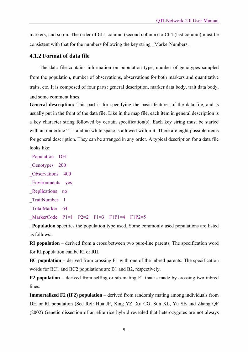
markers, and so on. The order of Ch1 column (second column) to Ch4 (last column) must be
consistent with that for the numbers following the key string _MarkerNumbers.
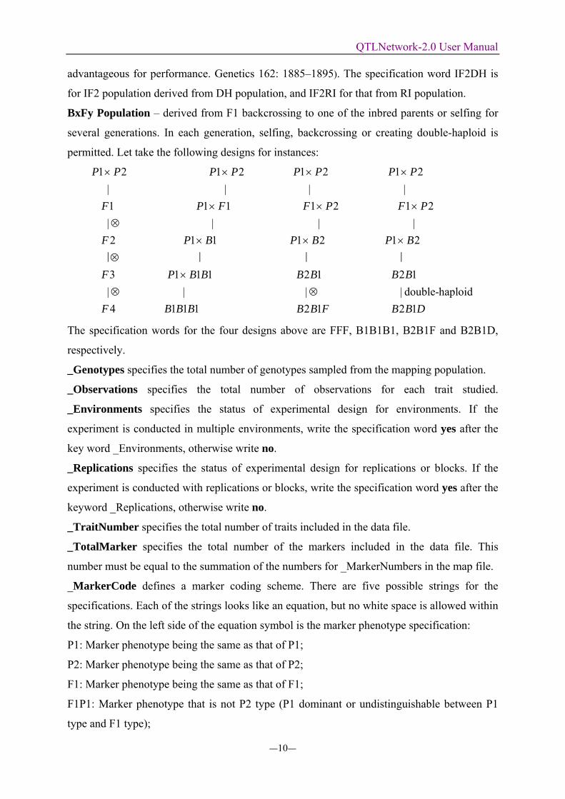
4.1.2 Format of data file
The data file contains information on population type, number of genotypes sampled
from the population, number of observations, observations for both markers and quantitative
traits, etc. It is composed of four parts: general description, marker data body, trait data body,
and some comment lines. General description: This part is for specifying the basic features of the data file, and is
usually put in the front of the data file. Like in the map file, each item in general description is
a key character string followed by certain specification(s). Each key string must be started
with an underline “_”, and no white space is allowed within it. There are eight possible items
for general description. They can be arranged in any order. A typical description for a data file
looks like:
_Population DH
_Genotypes 200
_Observations 400
_Environments yes
_Replications no
_TraitNumber 1
_TotalMarker 64
_MarkerCode P1=1 P2=2 F1=3 F1P1=4 F1P2=5
_Population specifies the population type used. Some commonly used populations are listed
as follows:
RI population – derived from a cross between two pure-line parents. The specification word
for RI population can be RI or RIL.
BC population – derived from crossing F1 with one of the inbred parents. The specification
words for BC1 and BC2 populations are B1 and B2, respectively.
F2 population – derived from selfing or sib-mating F1 that is made by crossing two inbred
lines.
Immortalized F2 (IF2) population – derived from randomly mating among individuals from
DH or RI population (See Ref: Hua JP, Xing YZ, Xu CG, Sun XL, Yu SB and Zhang QF
(2002) Genetic dissection of an elite rice hybrid revealed that heterozygotes are not always
QTLNetwork-2.0 User Manual
―10―
advantageous for performance. Genetics 162: 1885–1895). The specification word IF2DH is
for IF2 population derived from DH population, and IF2RI for that from RI population.
BxFy Population – derived from F1 backcrossing to one of the inbred parents or selfing for
several generations. In each generation, selfing, backcrossing or creating double-haploid is
permitted. Let take the following designs for instances:
1 2|1|2
3|4
P P
F
F
F
F
×
⊗
⊗
⊗
|
1 2|
1 1|
1 1
1 1 1|
1 1 1
P P
P F
P B
P B B
B B B
×
×
×
×|
1 2|1 2
|1 2
2 1|2 1
P P
F P
P B
B B
B B F
×
×
×
⊗
|
1 2|1 2
|1 2
2 1| double-haploid2 1
P P
F P
P B
B B
B B D
×
×
×|
The specification words for the four designs above are FFF, B1B1B1, B2B1F and B2B1D,
respectively.
_Genotypes specifies the total number of genotypes sampled from the mapping population.
_Observations specifies the total number of observations for each trait studied.
_Environments specifies the status of experimental design for environments. If the
experiment is conducted in multiple environments, write the specification word yes after the
key word _Environments, otherwise write no.
_Replications specifies the status of experimental design for replications or blocks. If the
experiment is conducted with replications or blocks, write the specification word yes after the
keyword _Replications, otherwise write no.
_TraitNumber specifies the total number of traits included in the data file.
_TotalMarker specifies the total number of the markers included in the data file. This
number must be equal to the summation of the numbers for _MarkerNumbers in the map file.
_MarkerCode defines a marker coding scheme. There are five possible strings for the
specifications. Each of the strings looks like an equation, but no white space is allowed within
the string. On the left side of the equation symbol is the marker phenotype specification:
P1: Marker phenotype being the same as that of P1;
P2: Marker phenotype being the same as that of P2;
F1: Marker phenotype being the same as that of F1;
F1P1: Marker phenotype that is not P2 type (P1 dominant or undistinguishable between P1
type and F1 type);
QTLNetwork-2.0 User Manual
―11―
F1P2: Marker phenotype that is not P1 type (P2 dominant or undistinguishable between P2
type and F1 type).
On the right side of the equation symbol is the code for the marker type. The marker
code should always be a single character (a number or a letter). The symbol dot “.” is used to
represent missing marker data or trait value. It is not necessary to specify codes for all
possible marker types except for F2 population. For example, if your marker data were
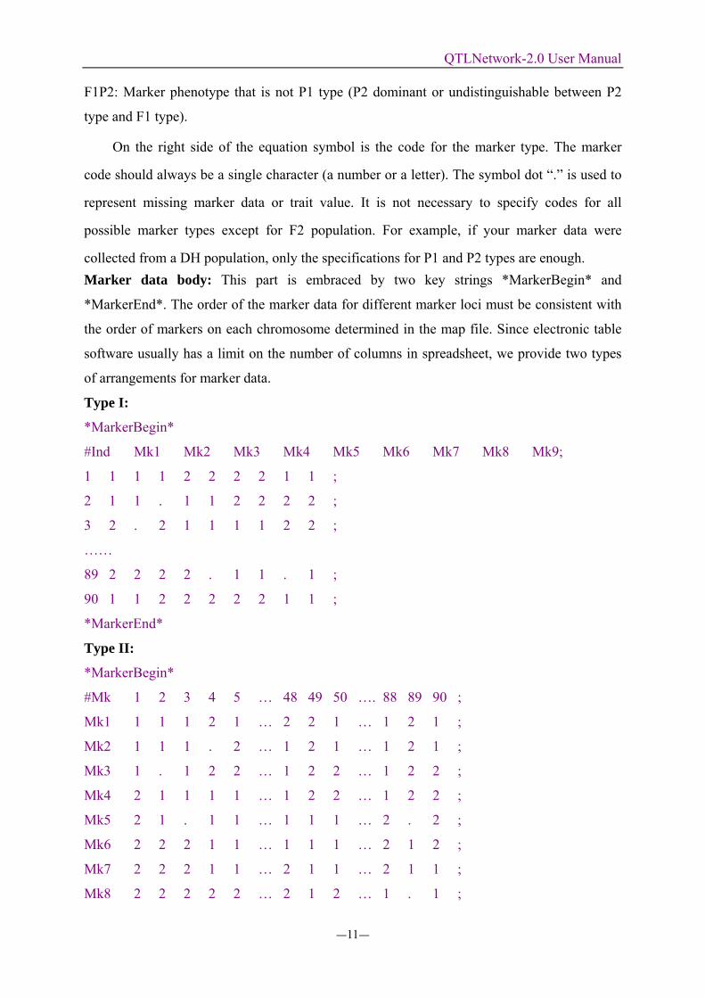
collected from a DH population, only the specifications for P1 and P2 types are enough. Marker data body: This part is embraced by two key strings *MarkerBegin* and
*MarkerEnd*. The order of the marker data for different marker loci must be consistent with
the order of markers on each chromosome determined in the map file. Since electronic table
software usually has a limit on the number of columns in spreadsheet, we provide two types
of arrangements for marker data.
Type I:
*MarkerBegin*
#Ind Mk1 Mk2 Mk3 Mk4 Mk5 Mk6 Mk7 Mk8 Mk9;
1 1 1 1 2 2 2 2 1 1 ;
2 1 1 . 1 1 2 2 2 2 ;
3 2 . 2 1 1 1 1 2 2 ;
……
89 2 2 2 2 . 1 1 . 1 ;
90 1 1 2 2 2 2 2 1 1 ;
*MarkerEnd*
Type II:
*MarkerBegin*
#Mk 1 2 3 4 5 … 48 49 50 …. 88 89 90 ;
Mk1 1 1 1 2 1 … 2 2 1 … 1 2 1 ;
Mk2 1 1 1 . 2 … 1 2 1 … 1 2 1 ;
Mk3 1 . 1 2 2 … 1 2 2 … 1 2 2 ;
Mk4 2 1 1 1 1 … 1 2 2 … 1 2 2 ;
Mk5 2 1 . 1 1 … 1 1 1 … 2 . 2 ;
Mk6 2 2 2 1 1 … 1 1 1 … 2 1 2 ;
Mk7 2 2 2 1 1 … 2 1 1 … 2 1 1 ;
Mk8 2 2 2 2 2 … 2 1 2 … 1 . 1 ;
QTLNetwork-2.0 User Manual
―12―
Mk9 1 2 2 2 2 … 2 2 2 … 2 1 1 ;
*MarkerEnd*
The two types of marker data arrangement are distinguished by a keyword placed at the
beginning of the send row, the keyword #Ind for type I and #Mk for type II. The marker
names and marker data must be arranged in the order given in the map file. Any list separator
is not allowed within the marker names. Each row must end with a semicolon “;”.
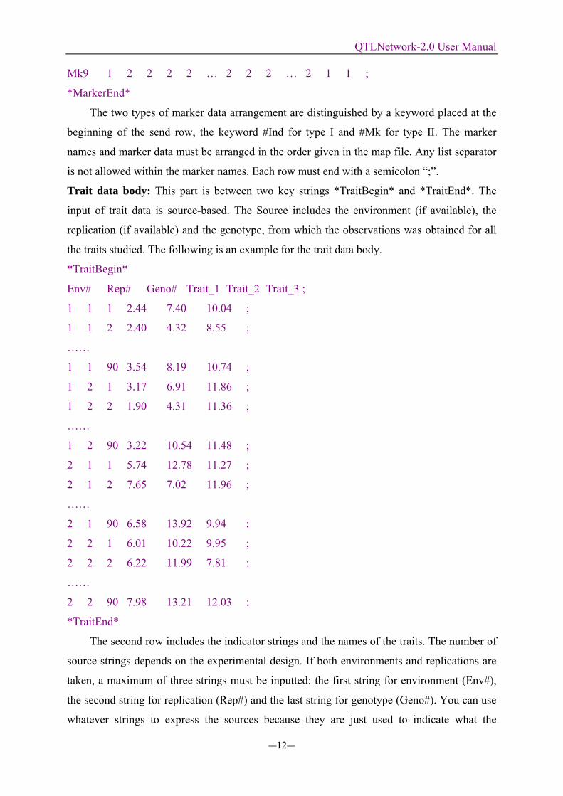
Trait data body: This part is between two key strings *TraitBegin* and *TraitEnd*. The
input of trait data is source-based. The Source includes the environment (if available), the
replication (if available) and the genotype, from which the observations was obtained for all
the traits studied. The following is an example for the trait data body.
*TraitBegin*
Env# Rep# Geno# Trait_1 Trait_2 Trait_3 ;
1 1 1 2.44 7.40 10.04 ;
1 1 2 2.40 4.32 8.55 ;
……
1 1 90 3.54 8.19 10.74 ;
1 2 1 3.17 6.91 11.86 ;
1 2 2 1.90 4.31 11.36 ;
……
1 2 90 3.22 10.54 11.48 ;
2 1 1 5.74 12.78 11.27 ;
2 1 2 7.65 7.02 11.96 ;
……
2 1 90 6.58 13.92 9.94 ;
2 2 1 6.01 10.22 9.95 ;
2 2 2 6.22 11.99 7.81 ;
……
2 2 90 7.98 13.21 12.03 ;
*TraitEnd*
The second row includes the indicator strings and the names of the traits. The number of
source strings depends on the experimental design. If both environments and replications are
taken, a maximum of three strings must be inputted: the first string for environment (Env#),
the second string for replication (Rep#) and the last string for genotype (Geno#). You can use
whatever strings to express the sources because they are just used to indicate what the
QTLNetwork-2.0 User Manual
―13―
numbers are in the columns below them. If the experiment is conducted without
environmental factor or replications, the corresponding column must be removed. And also, a
semicolon “;” is required at the end of each observation data row.
4.1.3 Other acceptable data formats
Our software could also accept the OUT data format of QTL Cartographer (*.map and
*.cro) and the data format of MapMaker/QTL (*.map and *.raw). It should be noted that the
marker number and order in the RAW file (*.raw) of MapMarker/QTL must be exactly
consistent with that in the map file. And the population type after the keyword “TYPE” must
have the same specifications as those of QTLNetwork, i.e. “F2” for F2 population, “DH” for
DH population, “RI” for Recombination inbred lines, “B1” and “B2” for backcross population
to P1 and P2.
4.2 Create new project with map and data files
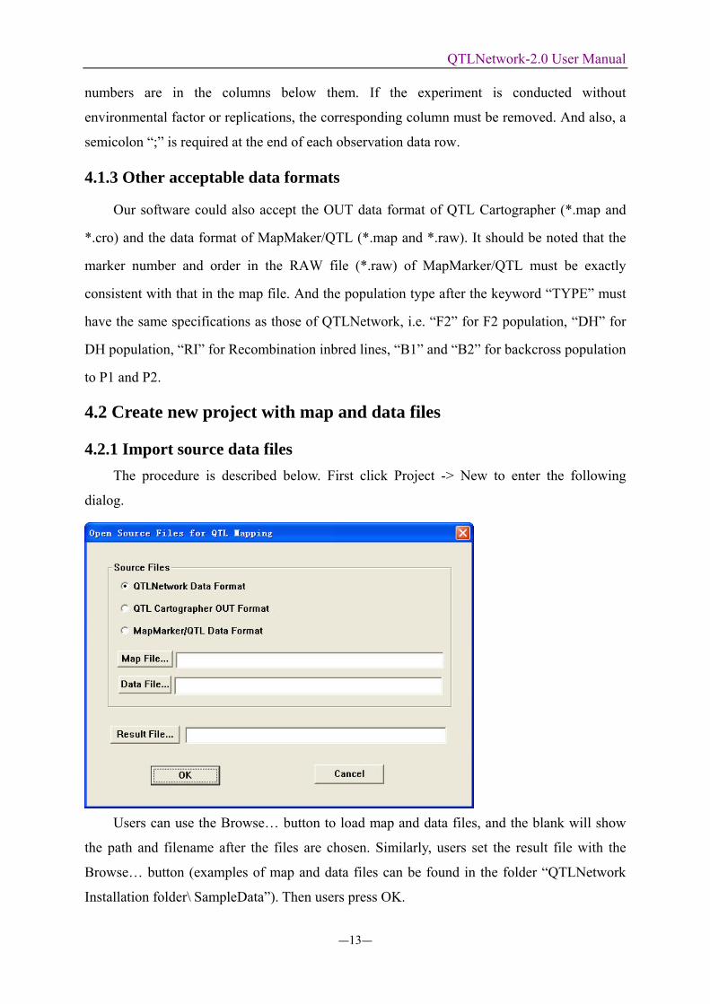
4.2.1 Import source data files The procedure is described below. First click Project -> New to enter the following
dialog.
Users can use the Browse… button to load map and data files, and the blank will show
the path and filename after the files are chosen. Similarly, users set the result file with the
Browse… button (examples of map and data files can be found in the folder “QTLNetwork
Installation folder\ SampleData”). Then users press OK.
QTLNetwork-2.0 User Manual
―14―
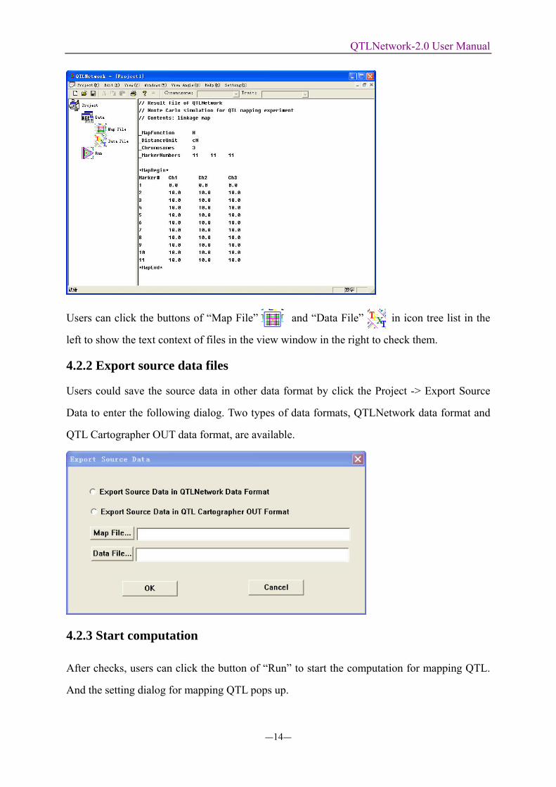
Users can click the buttons of “Map File” and “Data File” in icon tree list in the
left to show the text context of files in the view window in the right to check them.
4.2.2 Export source data files
Users could save the source data in other data format by click the Project -> Export Source
Data to enter the following dialog. Two types of data formats, QTLNetwork data format and
QTL Cartographer OUT data format, are available.
4.2.3 Start computation
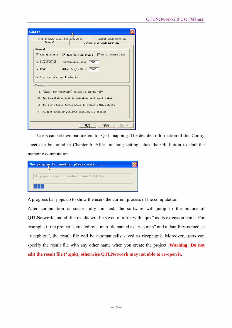
After checks, users can click the button of “Run” to start the computation for mapping QTL.
And the setting dialog for mapping QTL pops up.
QTLNetwork-2.0 User Manual
―15―
Users can set own parameters for QTL mapping. The detailed information of this Config
sheet can be found in Chapter 6. After finishing setting, click the OK button to start the
mapping computation.
A progress bar pops up to show the users the current process of the computation.
After computation is successfully finished, the software will jump to the picture of
QTLNetwork, and all the results will be saved in a file with “qnk” as its extension name. For
example, if the project is created by a map file named as “rice.map” and a data files named as
“riceph.txt”, the result file will be automatically saved as riceph.qnk. Moreover, users can
specify the result file with any other name when you create the project. Warning! Do not
edit the result file (*.qnk), otherwise QTLNetwork may not able to re-open it.
QTLNetwork-2.0 User Manual
―16―
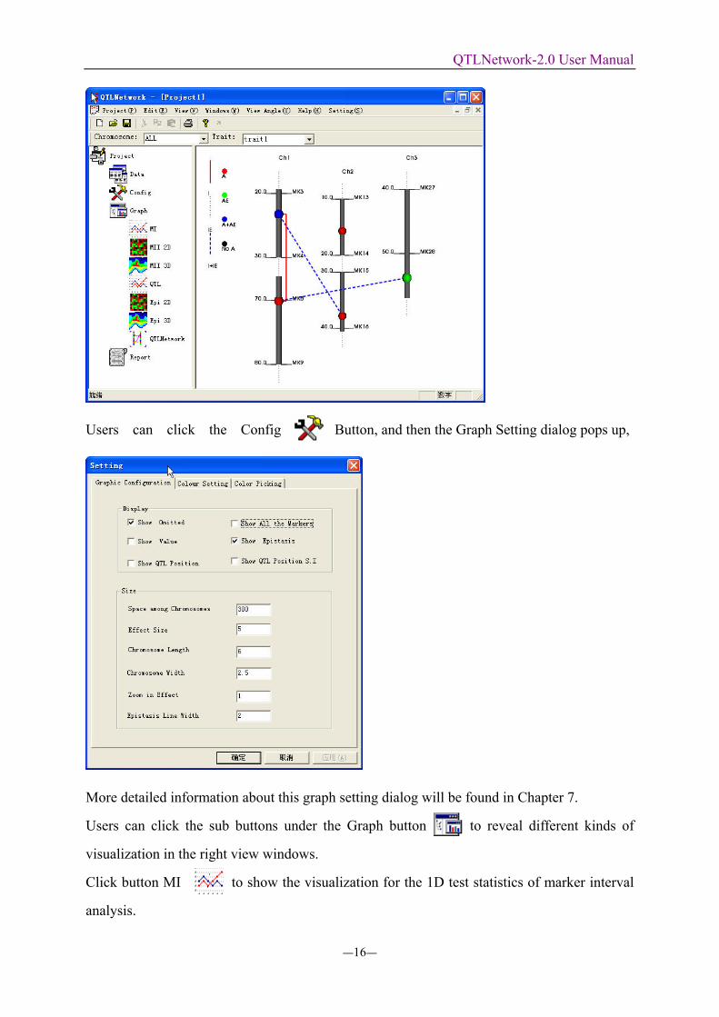
Users can click the Config Button, and then the Graph Setting dialog pops up,
More detailed information about this graph setting dialog will be found in Chapter 7.
Users can click the sub buttons under the Graph button to reveal different kinds of
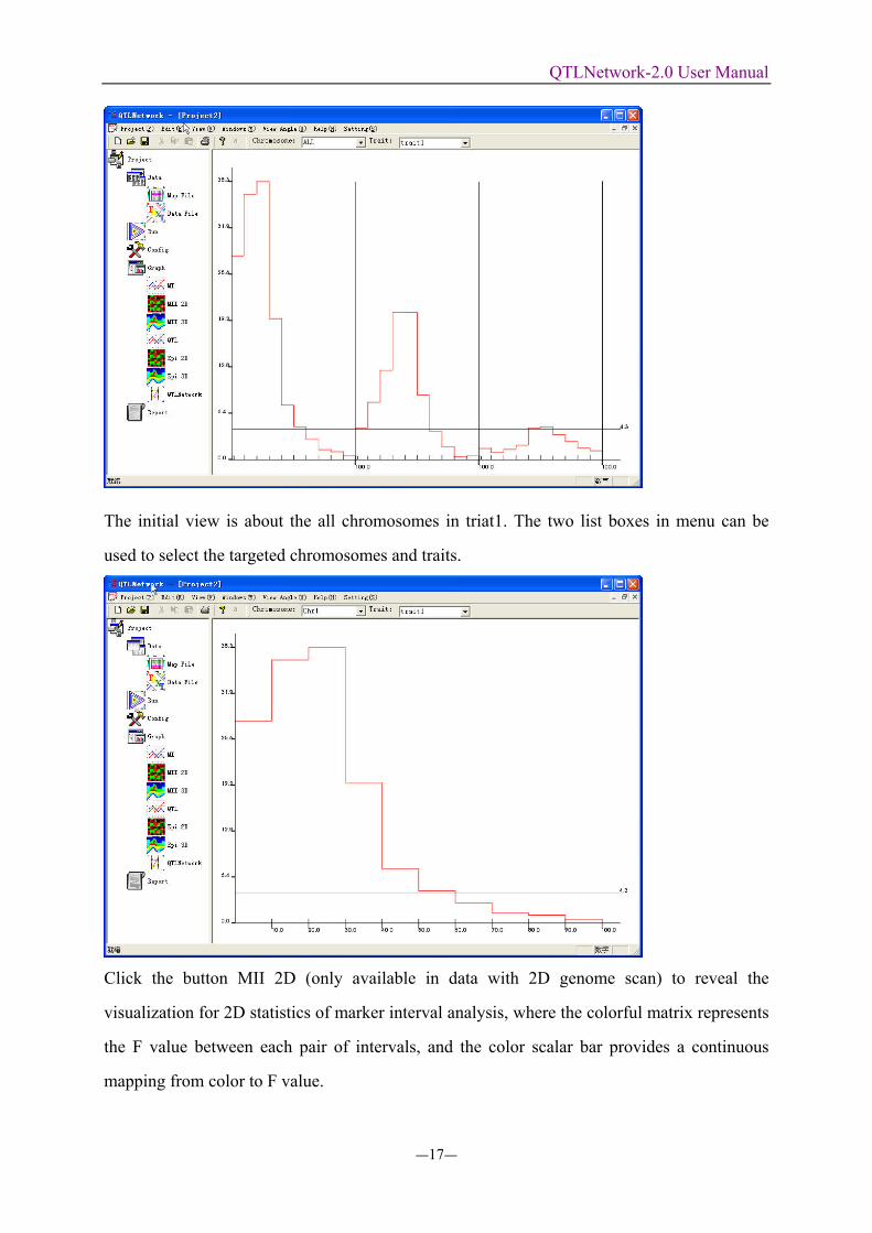
visualization in the right view windows.
Click button MI to show the visualization for the 1D test statistics of marker interval
analysis.
QTLNetwork-2.0 User Manual
―17―
The initial view is about the all chromosomes in triat1. The two list boxes in menu can be
used to select the targeted chromosomes and traits.
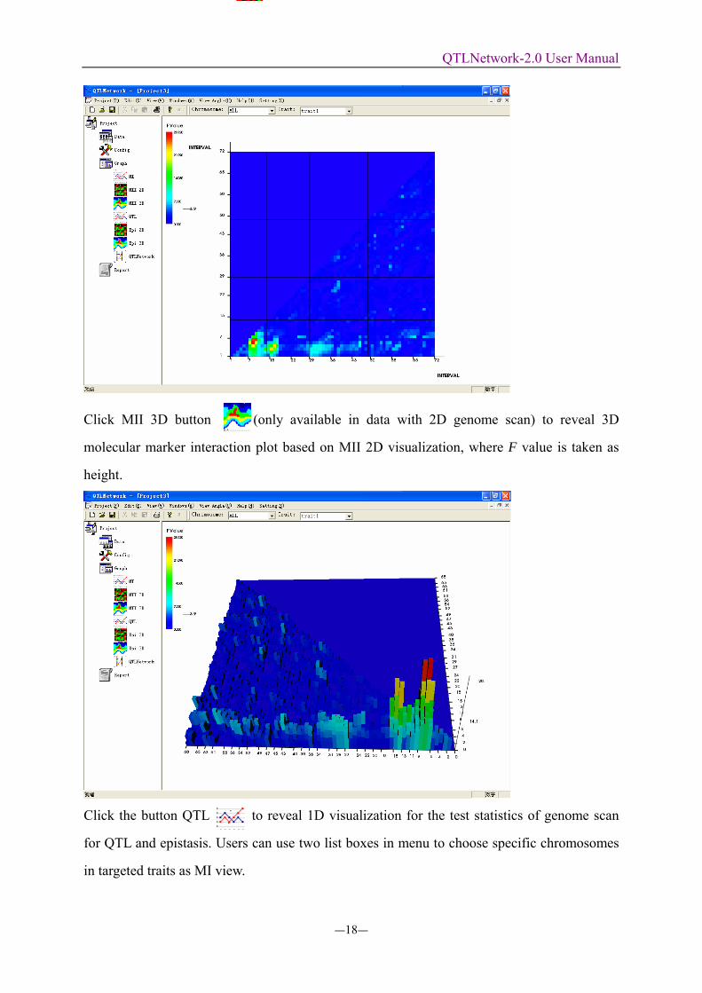
Click the button MII 2D (only available in data with 2D genome scan) to reveal the
visualization for 2D statistics of marker interval analysis, where the colorful matrix represents
the F value between each pair of intervals, and the color scalar bar provides a continuous
mapping from color to F value.
QTLNetwork-2.0 User Manual
―18―
Click MII 3D button (only available in data with 2D genome scan) to reveal 3D
molecular marker interaction plot based on MII 2D visualization, where F value is taken as
height.
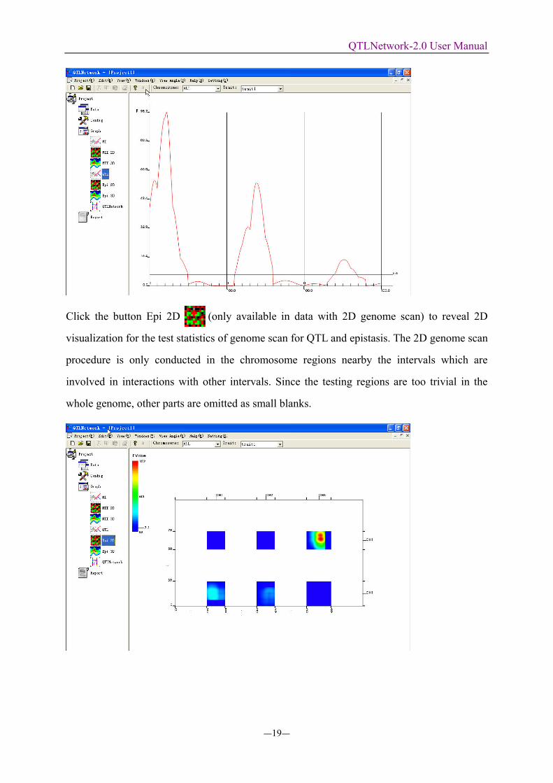
Click the button QTL to reveal 1D visualization for the test statistics of genome scan
for QTL and epistasis. Users can use two list boxes in menu to choose specific chromosomes
in targeted traits as MI view.
QTLNetwork-2.0 User Manual
―19―
Click the button Epi 2D (only available in data with 2D genome scan) to reveal 2D
visualization for the test statistics of genome scan for QTL and epistasis. The 2D genome scan
procedure is only conducted in the chromosome regions nearby the intervals which are
involved in interactions with other intervals. Since the testing regions are too trivial in the
whole genome, other parts are omitted as small blanks.
QTLNetwork-2.0 User Manual
―20―
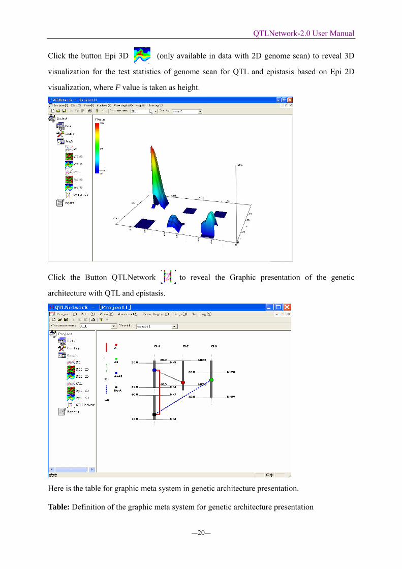
Click the button Epi 3D (only available in data with 2D genome scan) to reveal 3D
visualization for the test statistics of genome scan for QTL and epistasis based on Epi 2D
visualization, where F value is taken as height.
Click the Button QTLNetwork to reveal the Graphic presentation of the genetic
architecture with QTL and epistasis.
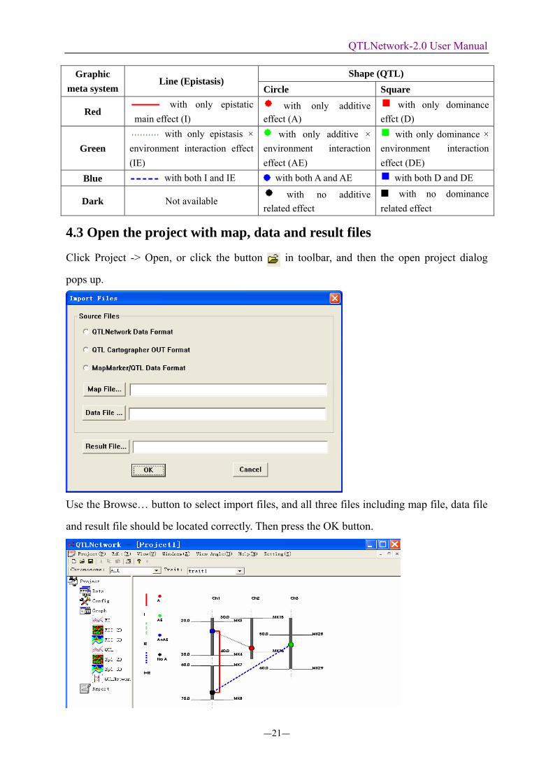
Here is the table for graphic meta system in genetic architecture presentation.
Table: Definition of the graphic meta system for genetic architecture presentation
QTLNetwork-2.0 User Manual
―21―
Shape (QTL) Graphic meta system
Line (Epistasis) Circle Square
Red with only epistatic
main effect (I) with only additive
effect (A) with only dominance
effct (D)
Green with only epistasis ×
environment interaction effect (IE)
with only additive × environment interaction effect (AE)
with only dominance × environment interaction effect (DE)
Blue with both I and IE with both A and AE with both D and DE
Dark Not available with no additive
related effect with no dominance
related effect
4.3 Open the project with map, data and result files
Click Project -> Open, or click the button in toolbar, and then the open project dialog
pops up.
Use the Browse… button to select import files, and all three files including map file, data file
and result file should be located correctly. Then press the OK button.
QTLNetwork-2.0 User Manual
―22―
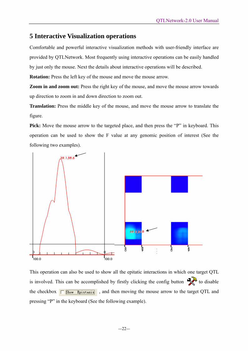
5 Interactive Visualization operations Comfortable and powerful interactive visualization methods with user-friendly interface are
provided by QTLNetwork. Most frequently using interactive operations can be easily handled
by just only the mouse. Next the details about interactive operations will be described.
Rotation: Press the left key of the mouse and move the mouse arrow.
Zoom in and zoom out: Press the right key of the mouse, and move the mouse arrow towards
up direction to zoom in and down direction to zoom out.
Translation: Press the middle key of the mouse, and move the mouse arrow to translate the
figure.
Pick: Move the mouse arrow to the targeted place, and then press the “P” in keyboard. This
operation can be used to show the F value at any genomic position of interest (See the
following two examples).
This operation can also be used to show all the epitatic interactions in which one target QTL
is involved. This can be accomplished by firstly clicking the config button to disable
the checkbox , and then moving the mouse arrow to the target QTL and
pressing “P” in the keyboard (See the following example).
QTLNetwork-2.0 User Manual
―23―
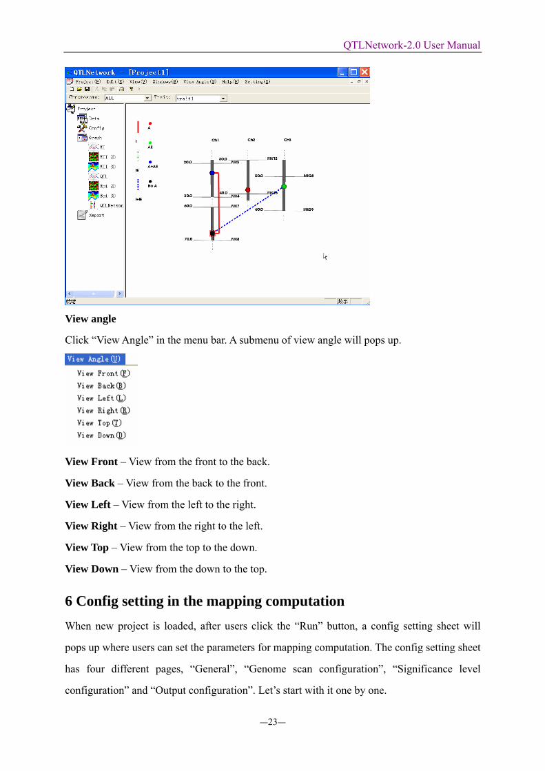
View angle
Click “View Angle” in the menu bar. A submenu of view angle will pops up.
View Front – View from the front to the back.
View Back – View from the back to the front.
View Left – View from the left to the right.
View Right – View from the right to the left.
View Top – View from the top to the down.
View Down – View from the down to the top.
6 Config setting in the mapping computation When new project is loaded, after users click the “Run” button, a config setting sheet will
pops up where users can set the parameters for mapping computation. The config setting sheet
has four different pages, “General”, “Genome scan configuration”, “Significance level
configuration” and “Output configuration”. Let’s start with it one by one.
QTLNetwork-2.0 User Manual
―24―
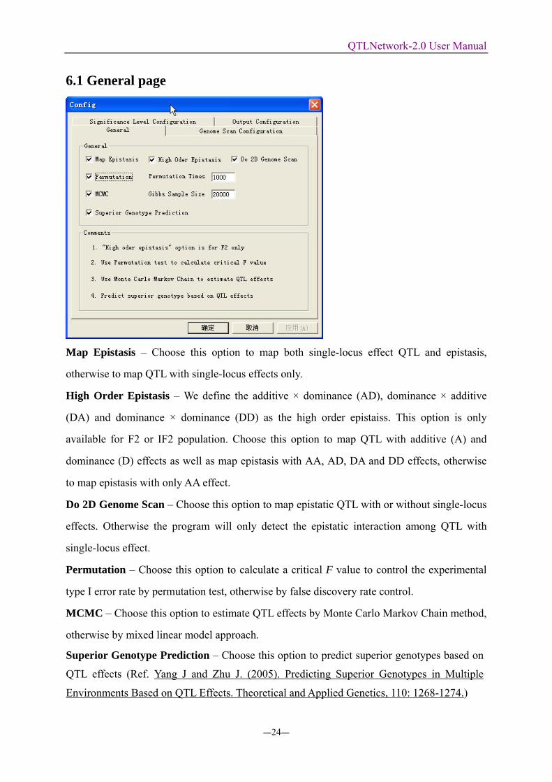
6.1 General page
Map Epistasis – Choose this option to map both single-locus effect QTL and epistasis,
otherwise to map QTL with single-locus effects only.
High Order Epistasis – We define the additive × dominance (AD), dominance × additive
(DA) and dominance × dominance (DD) as the high order epistaiss. This option is only
available for F2 or IF2 population. Choose this option to map QTL with additive (A) and
dominance (D) effects as well as map epistasis with AA, AD, DA and DD effects, otherwise
to map epistasis with only AA effect.
Do 2D Genome Scan – Choose this option to map epistatic QTL with or without single-locus
effects. Otherwise the program will only detect the epistatic interaction among QTL with
single-locus effect.
Permutation – Choose this option to calculate a critical F value to control the experimental
type I error rate by permutation test, otherwise by false discovery rate control.
MCMC – Choose this option to estimate QTL effects by Monte Carlo Markov Chain method,
otherwise by mixed linear model approach.
Superior Genotype Prediction – Choose this option to predict superior genotypes based on
QTL effects (Ref. Yang J and Zhu J. (2005). Predicting Superior Genotypes in Multiple
Environments Based on QTL Effects. Theoretical and Applied Genetics, 110: 1268-1274.)
QTLNetwork-2.0 User Manual
―25―
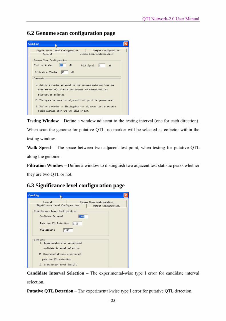
6.2 Genome scan configuration page
Testing Window – Define a window adjacent to the testing interval (one for each direction).
When scan the genome for putative QTL, no marker will be selected as cofactor within the
testing window.
Walk Speed – The space between two adjacent test point, when testing for putative QTL
along the genome.
Filtration Window – Define a window to distinguish two adjacent test statistic peaks whether
they are two QTL or not.
6.3 Significance level configuration page
Candidate Interval Selection – The experimental-wise type I error for candidate interval
selection.
Putative QTL Detection – The experimental-wise type I error for putative QTL detection.
QTLNetwork-2.0 User Manual
―26―
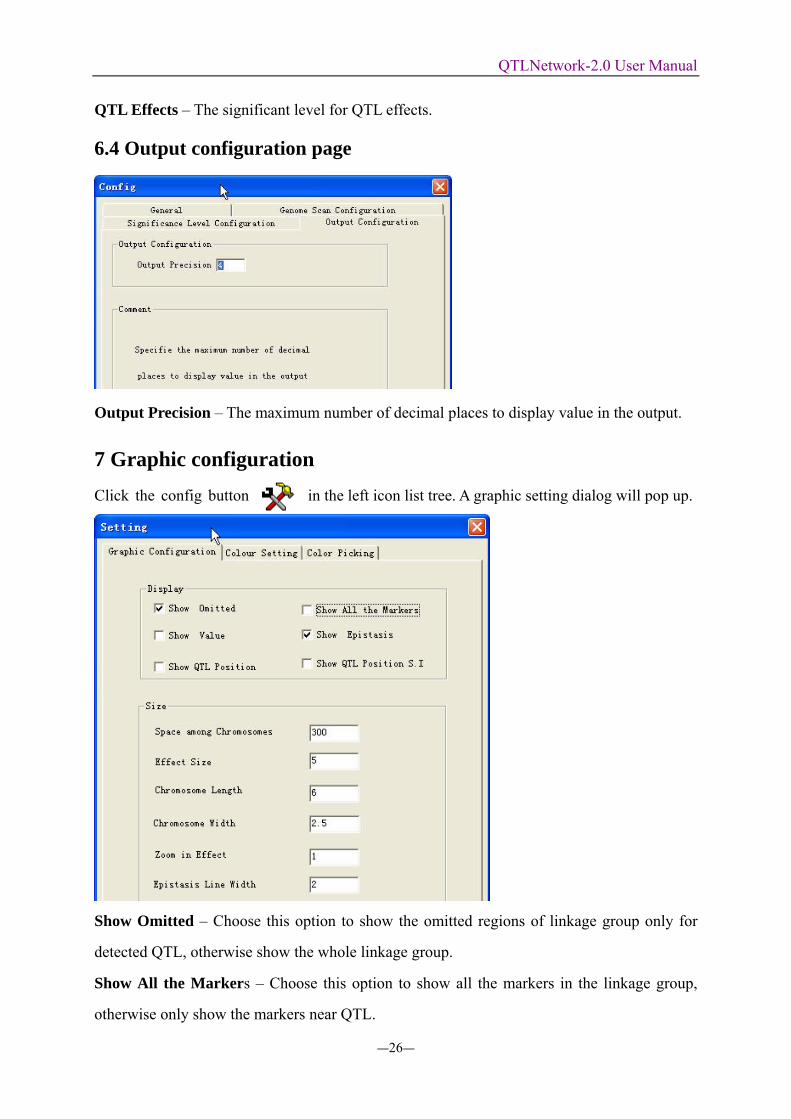
QTL Effects – The significant level for QTL effects.
6.4 Output configuration page
Output Precision – The maximum number of decimal places to display value in the output.
7 Graphic configuration Click the config button in the left icon list tree. A graphic setting dialog will pop up.
Show Omitted – Choose this option to show the omitted regions of linkage group only for
detected QTL, otherwise show the whole linkage group.
Show All the Markers – Choose this option to show all the markers in the linkage group,
otherwise only show the markers near QTL.
QTLNetwork-2.0 User Manual
―27―
Show Value – Choose this option to show the effect values of QTL and epistasis.
Show Epistasis – Choose this option to show the epistatic interaction among QTL.
Show QTL Position S.I. – Choose this option to show the support interval of QTL position.
Space among Chromosomes – The distance between two adjacent chromosomes.
Effect Size – The radius of the effect sphere.
Chromosome Length – The length of the chromosome column.
Chromosome Width – The width of the chromosome column.
Zoom in Effect –The scale size of effects in the QTL network graph.
Epistasis Line Width – The width of the epistasis line.
8 Save pictures and reports
8.1 Save pictures. QTLNetwork provides users easy-use interface to save pictures of all the graphs.
There are two different ways of saving pictures, “Save picture” and “Quick SP options”.
Save Picture – Click this item, a normal file dialog appears to help users to save the graph in
a targeted directory.
Quick SP – Click this item, the software will automatically save the graph in a picture file,
which will be named the data filename plus the serial number. The serial number increases
from 1 to N.
8.2 Save and Understand the Text Reports Click the “Edit” button in the menu bar, and then click “Save Report”. A normal file dialog
appears to help users to save the QTL mapping result in text format in a targeted directory.
The report is presented in six parts (if all the options have been chosen in the config dialog
before computing) each of which start with a key word.
Part 1 _variance_components (partition the variance components of phenotype
QTLNetwork-2.0 User Manual
―28―
variation)
V(G)/V(P)– variance of genetic main effects divided by phenotypic variance;
V(E)/V(P)– variance of environmental effects divided by phenotypic variance;
V(GE)/V(P)– variance of genotype-by-environment interaction effects divided by phenotypic
variance;
V(e) /V(P)– variance of residual effects divided by phenotypic variance;
V(p)– phenotypic variance.
Part 2 _QTL (mapping results of single-locus effect QTL)
QTL– QTL is named with the relevant chromosome and the marker intervals. For example, if
a QTL is named as 3-6, it is means that this QTL locates at the 6th marker interval of the 3th
chromosome.
Interval – The flanking markers of QTL.
Position – The distance between QTL and the first marker of the relevant chromosome.
Range – The support interval of QTL position.
A – The estimated additive effect.
D –The estimated dominance effect.
AE – The predicted additive by environment interaction effect.
DE –The predicted dominance by environment interaction effect.
SE and P-Value –The standard error of estimated or predicted QTL effect and P-value.
Part 3 _QTL_heritability (heritabilities of QTL effects)
h^2(a)– The heritability of additive effect.
h^2(d)– The heritability of dominance effect.
h^2(ae)– The heritability of additive by environment interaction effects.
h^2(de)– The heritability of dominance by environment interaction effects.
Part 4 _epistasis (mapping results of epistasis)
QTL_i and QTL_j– The two QTL involved in epistatic interaction.
interval_i– The flanking markers of QTL_i.
position_i– The distance between QTL_i and the first marker of the relevant chromosome
QTLNetwork-2.0 User Manual
―29―
range_i– The position support interval of QTL_i.
interval_j– The flanking markers of QTL_j.
position_j– The distance between QTL_j and the first marker of the relevant chromosome
range_j– The position support interval of QTL_j.
AA – The estimated additive by additive effect.
AD – The estimated additive by dominance effect.
DA –The estimated dominance by additive effect.
DD – The estimated dominance by dominance effect.
AAE – The predicted aa by environment interaction effect.
ADE – The predicted ad by environment interaction effect.
DAE – The predicted da by environment interaction effect.
DDE –The predicted dd by environment interaction effect.
SE and P-Value –The standard error of estimated or predicted QTL effect and P-value.
Part 5 _epistasis_heritability (heritabilities of epistatic effects)
h^2(aa)– The heritability of additive by additive effect.
h^2(ad)– The heritability of additive by dominance effect.
h^2(da)– The heritability of dominance by additive effect.
h^2(dd)– The heritability of dominance by dominance effect.
h^2(aae)– The heritability of aa by environment interaction effects.
h^2(ade)– The heritability of ad by environment interaction effects.
h^2(dae)– The heritability of da by environment interaction effects.
h^2(ade)– The heritability of dd by environment interaction effects.
Part 6 _genotype_value (genetic effects of the two parents, the F1 hybrid and the predicted
superior genotypes)
G– general genetic effects of P1, P2 and F1 hybrid as well as the predicted general superior
lines and general superior hybrids.
G+GE– total genetic effects of P1, P2 and F1 hybrid in a specific environment as well as the
predicted superior lines and superior hybrids in that environment.
The notation (+) and (–) denote the superior genotypes are predicted to get the maximum and

QTLNetwork-2.0 User Manual
―30―
minimum genetic effects, respectively.
Part 7 _superior_genotype (QTL geneotypes of the predicted superior genotypes)
G– specifies the general genetic effects of P1, P2 and F1 hybrid as well as the predicted
general superior genotypes.
G+GE– specifies the total genetic effects of P1, P2 and F1 hybrid in a specific environment as
well as the predicted superior genotype in that environment.