QSAR of corrosion inhibitors by genetic function ... · QSAR of corrosion inhibitors by genetic...

J. Mater. Environ. Sci. 7 (6) (2016) 2121-2136 Khaled et al.

ISSN : 2028-2508

CODEN: JMESC

2121

QSAR of corrosion inhibitors by genetic function approximation, neural

network and molecular dynamics simulation methods

K.F. Khaled

*1,2 N.M.Al-Nofai

*1, N. S. Abdel-Shafi

2,3

1Chemistry Department, Faculty of Science, Taif University, Saudi Arabia

2Electrochemistry Research Laboratory, Chemistry Department, Faculty of Education, Ain Shams Univ., Roxy, Cairo, Egypt

3Chemistry Department, Faculty of Science, Hail University, Hail, Saudi Arabia

Received 23 Jan 2016, Revised 23 Mar 2016, Accepted 08 Apr 2016

*Corresponding author. E-mail: [email protected] (K. F. Khaled) & [email protected] (N. M. Al-Nofai);

Abstract Correlations between the calculated physicochemical descriptors and corrosion inhibition efficiency for furan

derivatives against iron corrosion in HCl solutions were examined using quantitative structure–activity

relationship (QSAR) paradigm, genetic function approximation (GFA) and neural network analysis (NNA)

techniques. The quantum chemical indices were calculated, the energy of the highest occupied molecular orbital

(EHOMO), the energy of the lowest unoccupied molecular orbital (ELUMO), Binding energy, Molecular sizes (area

and volume) for the seventeen furan derivatives. Molecular dynamics (MD) method and density functional theory

have been used to study adsorption behavior of these inhibitors on Fe surface. High correlation was obtained with

the multivariate correlation, i.e. all the indices combined together, where the prediction power was very high for

GFA and NNA. The GFA and NNA algorithm has been applied to these published data sets to demonstrate it is

an effective tool for doing QSAR. The molecular dynamics simulations results indicated that the furan derivatives

could adsorb on the Fe surface firmly through the hetero-atoms.

Keywords: Acid corrosion inhibitor; Modeling studies; QSAR; Genetic Function Approximation algorithm; Neural

Network Analysis.

1. Introduction

A subject of intense interest in corrosion science research is the effect of molecular structure of the corrosion

inhibitor molecule on its inhibition efficiency [1-5]. Quantitative structure activity relationship (QSAR) has been

derived for several series of active corrosion inhibitors [6-9].

Some organic compounds have been used as corrosion inhibitors for many metals and alloys. It has been known

that organic inhibitor usually interacts electrostatically with the metal surface. It includes electrons transfer from

the organic compounds to metal surface. Also, it forms coordinate covalent bond during chemical adsorption

process [10-12].

Recently, theoretical chemical calculations have been used, such as quantum chemical calculations, to

illustrate the mechanism of corrosion inhibition [13-17].

In this study theoretical measurements go far beyond the experimental research. The method of quantum chemical

calculations has been widely used as a powerful tool for studying the reaction mechanisms of corrosion inhibition.


ISSN : 2028-2508

CODEN: JMESC

2122

The structural parameters such as the frontier molecular orbital (MO) energy HOMO (highest occupied molecular

orbital) and LUMO (lowest unoccupied molecular orbital) and molecular volume/area [8]. The quantitative

structure-activity relationship (QSAR) is a relationship between descriptors characterizing the structure properties

of corrosion inhibitors against their corrosion inhibition efficiencies.

QSAR correlates and predicts physical and chemical properties of chemicals and plays an important role in

effective assessment of organic inhibitors. The application of QSAR in corrosion research has been reported [18,

19].

Genetic function approximation (GFA) algorithm offers a new approach to the problem of building quantitative

structure-activity relationship (QSAR) and quantitative structure property relationship (QSPR) models [20-22].

Replacing regression analysis with the GFA algorithm allows the construction of models competitive with or

superior to those produced by standard techniques. GFA makes available additional information not provided by

other techniques. GFA provides multiple models, where the populations of the models are created by evolving

random initial models using a genetic algorithm [23].

Neural network (NN) analysis method which is an artificial intelligence approach to mathematical modeling.

Neutral networks are inspired by the way the human brain works. The brain consists of billions of neurons, which

are linked together into a complex network. A neuron communicates with another by sending an electrical signal

along an axon, which is a long nerve fiber that connects to the second neuron at a synapse [24, 25]. Each neuron

acts as an information processing element because the electrical signals sent out by one neuron depend on the

strength of the incoming signals at its synapses [24, 26]. Neural network analysis is a sophisticated model-

building technique capable of modeling data may be better represented by non-linear functions. Corrosion is a

complex non-linear phenomenon that is too complex to be described by analytical methods or empirical rules

which make it an ideal phenomenon to be studied using artificial neural networks [24, 27].

The main purpose of this work is to build a quantitative structure–activity relationship (QSAR) using (GFA) and

(NNA) between the structural properties and the inhibition efficiencies of seventeen furan derivatives. Also, the

aim of this work is to simulate the adsorption of an example of furan derivative molecules on iron (111) surface

computationally as well as generating adsorption configurations to obtain a ranking of the energies for each

generated configuration, thereby indicating the preferred adsorption sites [8].

2. Computational and statistical details The quantum chemical calculations were performed using the generalized gradient approximation (GGA)

within the density functional theory was conducted with the software package DMol3 in Materials Studio of

BIOVIA. To optimize the molecule geometry and to obtain the quantum chemical parameters, parametric Method

(PM3) and semi-empirical method were employed [10]. Complete geometric optimization of all stationary points

for the seventeen investigated furan derivatives. The double numerical with polarization (DNP) basis set and the

(PWC) exchange correlation functional were conducted in all calculations, since this was the best set available in

DMol3. This basis set is known to provide accurate electronic properties and geometries for wide range of organic

compounds. The optimization was repeated until minimum energy reached. The quantum chemical indices were

calculated: the energy of the highest occupied molecular orbital (EHOMO), the energy of the lowest unoccupied

molecular orbital (ELUMO), Binding energy, Molecular sizes (area and volume) of all compounds for the seventeen

furan derivatives using QSAR model.

To get the lower energy adsorption sites on the iron surface and to examine the favored adsorption of the

studied inhibitors, the studied furan derivatives have been simulated as adsorbate on iron surface (111) substrate

[28]. Monte Carlo method has been used to calculate the binding energy and the adsorption density of the studied

inhibitors. In this computational study, possible adsorption configurations have been identified by carrying out

Monte Carlo searches of the configurationally space of the iron/ furan derivatives inhibitor system as the

temperature is slowly decreased [28].

The studied furan derivatives, the adsorbates, were constructed and their energy was optimized using Forcite

classical simulation engine [28].


ISSN : 2028-2508

CODEN: JMESC

2123

The geometry optimization process is carried out using an iterative process, in which the atomic

coordinates are adjusted until the total energy of a structure is minimized, i.e., it corresponds to a local minimum

in the potential energy surface [28, 29]. Geometry optimization is based on reducing the magnitude of calculated

forces until they become smaller than defined convergence tolerances [28]. The forces on the atoms in the studied

inhibitors are calculated from the potential energy expression and will, therefore, depend on the force field that is

selected [28]. Materials Studio software is used to perform the MD simulation of the interaction between the

studied inhibitor molecule and iron (111) surface [30]. The size of the area above the electrode surface (vacuum

slab) must be enough (15 Å) that the non-bond calculation for the adsorbate does not interact with the periodic

image of the bottom layer of atoms in the surface. After minimizing the Fe (111) surface and the furan derivatives

inhibitor molecules, the corrosion system will be built by layer builder to place the inhibitor molecules on Fe

(111) surface, and the COMPASS (condensed phase optimized molecular potentials for atomistic simulation

studies) force field was used to simulate the behaviors of these molecules on the Fe (111) surface [28]. To model

the adsorption of the inhibitor molecules onto Fe (111) surface, adsorption locator module in Materials Studio

have been used 7[31], and thus provide access to the energetic of the adsorption and its effects on the inhibition

efficiencies of the studied. The following equation was used to calculate the binding energy, Ebinding between the

studied inhibitors and Fe (111) surface [32].

𝐸𝑏𝑖𝑛𝑑𝑖𝑛𝑔 = 𝐸𝑡𝑜𝑡𝑎𝑙 − 𝐸𝑠𝑢𝑟𝑓𝑎𝑐𝑒 + 𝐸𝑖𝑛𝑕𝑖𝑏𝑖𝑡𝑖𝑜𝑛 (1)

Where (Etotal ) is the total energy of the inhibitor and surface, (Esurface ) is the energy of the surface without the

inhibitor, and (Einhibition ) is the energy of the inhibitor without the surface.

The Genetic Function Approximation GFA algorithm detailed description has been described elsewhere

[28, 33]. This technique has a number of important advantages over other standard regression analysis techniques.

It forms multiple models instead of a single model [28, 34]. It automatically selects which features are to be used

in the models. It is better at discovering combinations of features that take advantage of correlations between

multiple features [28]. GFA incorporates Friedman's LOF error measure, which estimates the most appropriate

number of features, resists over-fitting, and allows control over the smoothness of fit. Also, it can use a larger

variety of equation term types in construction of its models and finally, it provides, through study of the evolving

models, additional information not available from standard regression analysis [28, 34].

The structure of the artificial neural network was described elsewhere [24]. It consists of layers. The input

layer(s), hidden layers and output layer. The input layer is used to introduce the input (predictor) variables to the

network. The upper layer is the output layer. The outputs of the nodes in this layer represent the predictions made

by the network for the response variables. The network also includes hidden layers with several nodes. Each node

(other than those in the input layer) takes as its input a transformed linear combination of the outputs from the

nodes in the layer below it. This input is then passed through a transfer function to calculate the output of the

node. The transfer function is an S-shaped sigmoid function which is used by QSAR. S-shaped sigmoid function

is chosen because it is smooth and easily differentiable, features that help the algorithm that is used to train the

network [24, 35].

3. Inhibitor

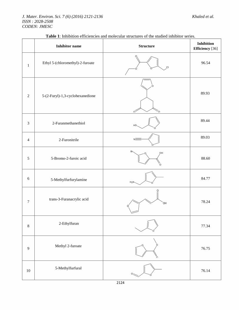
The dataset used in this study consisted of seventeen furan derivatives used as corrosion inhibitors and their

calculated corrosion inhibition extracted from literature [36]. A brief summary for the determination of corrosion

inhibition of mild steel in 1 M HCl in the presence of the furan derivatives are presented as elsewhere [36].

Potentiodynamic polarization measurements were carried out at (25±1°C) using 250 ml of 1.0 M HCl solution

without and with the addition of 0.005 M of the inhibitors.

Polarization measurements was conducted in potential range -0.25 and +0.25 V with respect to open circuit

potential in Autolab potentiostat/Galvanostat using a standard three electrode corrosion cell [36].


ISSN : 2028-2508

CODEN: JMESC

2124

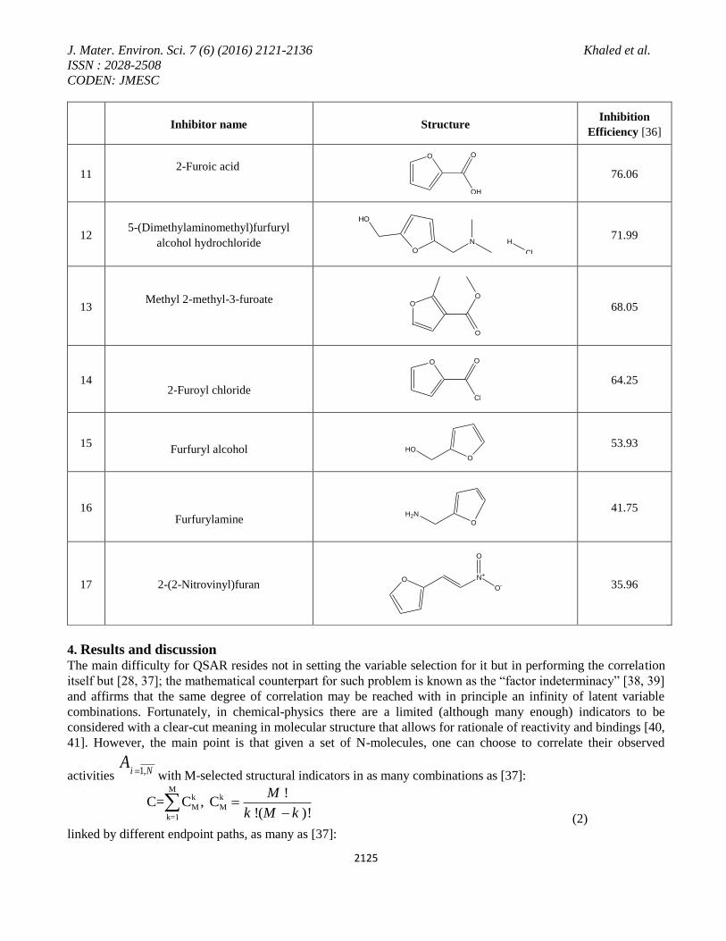
Table 1: Inhibition efficiencies and molecular structures of the studied inhibitor series.

Inhibition

Efficiency [36] Structure Inhibitor name

96.54

O

O

OCl

Ethyl 5-(chloromethyl)-2-furoate

1

89.93

OO

O

5-(2-Furyl)-1,3-cyclohexanedione 2

89.44

O

HS

2-Furanmethanethiol 3

89.03

O

N

2-Furonitrile 4

88.60

O

O

OHBr

5-Bromo-2-furoic acid 5

84.77 H2N O

5-Methylfurfurylamine

6

78.24 O

O

OH

trans-3-Furanacrylic acid

7

77.34 O

2-Ethylfuran

8

76.75 O

O

O

Methyl 2-furoate

9

76.14 O

O

5-Methylfurfural

10


ISSN : 2028-2508

CODEN: JMESC

2125

Inhibition

Efficiency [36] Structure Inhibitor name

76.06

O O

OH

2-Furoic acid

11

71.99

O

N

HO

H

Cl

5-(Dimethylaminomethyl)furfuryl

alcohol hydrochloride 12

68.05 O

O

O

Methyl 2-methyl-3-furoate

13

64.25

O O

Cl 2-Furoyl chloride

14

53.93

O

HO

Furfuryl alcohol

15

41.75 H2N

O Furfurylamine

16

35.96 O N+

O

O-

2-(2-Nitrovinyl)furan 17

4. Results and discussion The main difficulty for QSAR resides not in setting the variable selection for it but in performing the correlation

itself but [28, 37]; the mathematical counterpart for such problem is known as the “factor indeterminacy” [38, 39]

and affirms that the same degree of correlation may be reached with in principle an infinity of latent variable

combinations. Fortunately, in chemical-physics there are a limited (although many enough) indicators to be

considered with a clear-cut meaning in molecular structure that allows for rationale of reactivity and bindings [40,

41]. However, the main point is that given a set of N-molecules, one can choose to correlate their observed

activities 1,i NA

with M-selected structural indicators in as many combinations as [37]: M

k k

M M

k=1

!C= C , C

!( )!

M

k M k

(2)

linked by different endpoint paths, as many as [37]:


ISSN : 2028-2508

CODEN: JMESC

2126

1

M k

MkK C

(3)

indexing the numbers of paths built from connected distinct models with orders (dimension of correlation) from

k=1 to k=M [37].

In the present study we developed the best QSAR model to explain the correlations between the

physicochemical parameters and corrosion inhibition efficiency for 17 furan derivatives used as corrosion

inhibitor extracted from the literature [36].

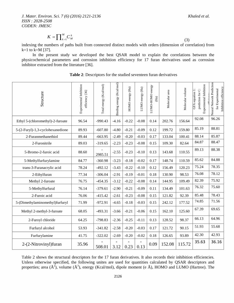
Table 2: Descriptors for the studied seventeen furan derivatives

Str

uct

ure

Exp

erim

enta

l In

hib

itio

n

effi

cien

cy [

36

]

To

tal

ener

gy (

Kca

l/m

ol)

Bin

din

g e

ner

gy

(K

cal/

mo

l)

HO

MO

en

erg

y (

Ha)

LU

MO

ener

gy

(H

a)

LU

MO

-HO

MO

ener

gy

(Ha)

Mole

cula

r ar

ea

Mole

cula

r vo

lum

e

GF

A e

qu

atio

n 1

:

pre

dic

tion

fo

r C

:

Exp

erim

enta

l In

hib

itio

n

effi

cien

cy

Neu

ral

Net

wo

rk P

red

icti

on

for

Ex

per

imen

tal

Inhib

itio

n e

ffic

ien

cy

Ethyl 5-(chloromethyl)-2-furoate 96.54 -990.43 -4.16 -0.22 -0.08 0.14 202.76 156.64 92.08 96.26

5-(2-Furyl)-1,3-cyclohexanedione 89.93 -607.80 -4.80 -0.21 -0.09 0.12 199.72 159.80 85.19 88.81

2-Furanmethanethiol 89.44 -663.95 -2.49 -0.20 -0.03 0.17 133.04 100.41 88.14 85.87

2-Furonitrile 89.03 -319.65 -2.23 -0.23 -0.08 0.15 109.30 82.64 84.87 88.47

5-Bromo-2-furoic acid 88.60 -

2985.51 -2.55 -0.23 -0.10 0.13 143.68 110.55

89.13 88.38

5-Methylfurfurylamine 84.77 -360.98 -3.23 -0.18 -0.02 0.17 148.74 110.59 85.62 84.88

trans-3-Furanacrylic acid 78.24 -492.12 -3.43 -0.22 -0.10 0.12 156.49 120.23 75.24 78.35

2-Ethylfuran 77.34 -306.04 -2.91 -0.19 -0.01 0.18 130.90 98.53 76.08 78.12

Methyl 2-furoate 76.75 -454.35 -3.12 -0.22 -0.08 0.14 144.95 109.49 82.39 75.92

5-Methylfurfural 76.14 -379.61 -2.90 -0.21 -0.09 0.11 134.49 101.63 76.32 75.60

2-Furoic acid 76.06 -415.42 -2.61 -0.23 -0.08 0.15 121.82 92.39 85.48 78.43

5-(Dimethylaminomethyl)furfuryl 71.99 -972.91 -4.65 -0.18 -0.03 0.15 242.12 177.52 74.85 71.56

Methyl 2-methyl-3-furoate 68.05 -493.31 -3.66 -0.21 -0.06 0.15 162.10 125.60 67.39 69.65

2-Furoyl chloride 64.25 -798.83 -2.36 -0.25 -0.11 0.13 128.52 98.37 66.13 64.96

Furfuryl alcohol 53.93 -341.82 -2.58 -0.20 -0.03 0.17 121.72 90.15 51.93 55.68

Furfurylamine 41.75 -322.02 -2.69 -0.20 -0.02 0.18 126.65 93.89 42.30 42.93

2-(2-Nitrovinyl)furan 35.96 -

508.01

-

3.12

-

0.23

-

0.13 0.09 152.08 115.72

35.63 36.16

Table 2 shows the structural descriptors for the 17 furan derivatives. It also records their inhibition efficiencies.

Unless otherwise specified, the following unites are used for quantities calculated by QSAR descriptors and

properties; area (Å2), volume (Å

3), energy (Kcal/mol), dipole moment (e Å), HOMO and LUMO (Hartree). The


ISSN : 2028-2508

CODEN: JMESC

2127

atom volumes and surfaces model calculate surface areas and volumes of surfaces around atomistic structures

using the atom volumes and surfaces functionality of the Materials Studio software [30, 42].

Molecular area in Table 2, describes the volume inside the van der waals area of the molecular surface area

determines the extent to which a molecule exposes to the external environment [28]. This descriptor is related to

binding, transport, and solubility. Molecular volume in Table 2, describes the volume inside the van der waals

area of a molecule [28]. Total molecular dipole moment, this descriptor calculates the molecule dipole moments

from partial charges defined on the atoms of the molecule [28]. If no partial charges were defined, the molecular

dipole moment would be zero. Total energy, HOMO and LUMO energy have been described in our previous

studies in details [33].

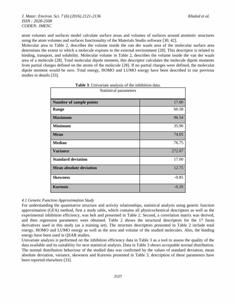
Table 3: Univariate analysis of the inhibition data.

Statistical parameters

Number of sample points 17.00

Range 60.58

Maximum 96.54

Minimum 35.96

Mean 74.05

Median 76.75

Variance 272.07

Standard deviation 17.00

Mean absolute deviation 12.75

Skewness -0.85

Kurtosis -0.29

4.1 Genetic Function Approximation Study

For understanding the quantitative structure and activity relationships, statistical analysis using genetic function

approximation (GFA) method, first a study table, which contains all physicochemical descriptors as well as the

experimental inhibition efficiency, was belt and presented in Table 2. Second, a correlation matrix was derived,

and then regression parameters were obtained. Table 2 shows the structural descriptors for the 17 furan

derivatives used in this study (as a training set). The structure descriptors presented in Table 2 include total

energy, HOMO and LUMO energy as well as the area and volume of the studied molecules. Also, the binding

energy have been used in QSAR studies.

Univariate analysis is performed on the inhibition efficiency data in Table 3 as a tool to assess the quality of the

data available and its suitability for next statistical analysis. Data in Table 3 shows acceptable normal distribution.

The normal distribution behaviour of the studied data was confirmed by the values of standard deviation, mean

absolute deviation, variance, skewness and Kurtosis presented in Table 3, description of these parameters have

been reported elsewhere [33].


ISSN : 2028-2508

CODEN: JMESC

2128

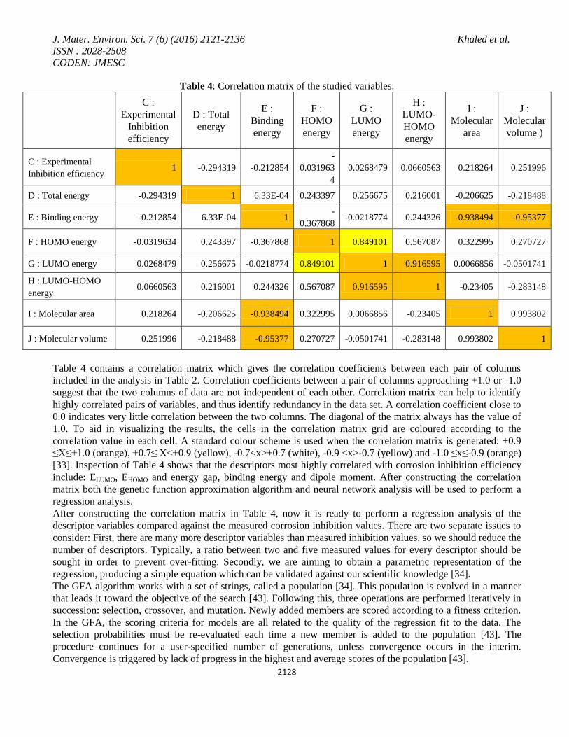
Table 4: Correlation matrix of the studied variables:

C :

Experimental

Inhibition

efficiency

D : Total

energy

E :

Binding

energy

F :

HOMO

energy

G :

LUMO

energy

H :

LUMO-

HOMO

energy

I :

Molecular

area

J :

Molecular

volume )

C : Experimental

Inhibition efficiency 1 -0.294319 -0.212854

-

0.031963

4

0.0268479 0.0660563 0.218264 0.251996

D : Total energy -0.294319 1 6.33E-04 0.243397 0.256675 0.216001 -0.206625 -0.218488

E : Binding energy -0.212854 6.33E-04 1 -

0.367868 -0.0218774 0.244326 -0.938494 -0.95377

F : HOMO energy -0.0319634 0.243397 -0.367868 1 0.849101 0.567087 0.322995 0.270727

G : LUMO energy 0.0268479 0.256675 -0.0218774 0.849101 1 0.916595 0.0066856 -0.0501741

H : LUMO-HOMO

energy 0.0660563 0.216001 0.244326 0.567087 0.916595 1 -0.23405 -0.283148

I : Molecular area 0.218264 -0.206625 -0.938494 0.322995 0.0066856 -0.23405 1 0.993802

J : Molecular volume 0.251996 -0.218488 -0.95377 0.270727 -0.0501741 -0.283148 0.993802 1

Table 4 contains a correlation matrix which gives the correlation coefficients between each pair of columns

included in the analysis in Table 2. Correlation coefficients between a pair of columns approaching +1.0 or -1.0

suggest that the two columns of data are not independent of each other. Correlation matrix can help to identify

highly correlated pairs of variables, and thus identify redundancy in the data set. A correlation coefficient close to

0.0 indicates very little correlation between the two columns. The diagonal of the matrix always has the value of

1.0. To aid in visualizing the results, the cells in the correlation matrix grid are coloured according to the

correlation value in each cell. A standard colour scheme is used when the correlation matrix is generated: +0.9

≤X≤+1.0 (orange), +0.7≤ X<+0.9 (yellow), -0.7<x>+0.7 (white), -0.9 <x>-0.7 (yellow) and -1.0 ≤x≤-0.9 (orange)

[33]. Inspection of Table 4 shows that the descriptors most highly correlated with corrosion inhibition efficiency

include: ELUMO, EHOMO and energy gap, binding energy and dipole moment. After constructing the correlation

matrix both the genetic function approximation algorithm and neural network analysis will be used to perform a

regression analysis.

After constructing the correlation matrix in Table 4, now it is ready to perform a regression analysis of the

descriptor variables compared against the measured corrosion inhibition values. There are two separate issues to

consider: First, there are many more descriptor variables than measured inhibition values, so we should reduce the

number of descriptors. Typically, a ratio between two and five measured values for every descriptor should be

sought in order to prevent over-fitting. Secondly, we are aiming to obtain a parametric representation of the

regression, producing a simple equation which can be validated against our scientific knowledge [34].

The GFA algorithm works with a set of strings, called a population [34]. This population is evolved in a manner

that leads it toward the objective of the search [43]. Following this, three operations are performed iteratively in

succession: selection, crossover, and mutation. Newly added members are scored according to a fitness criterion.

In the GFA, the scoring criteria for models are all related to the quality of the regression fit to the data. The

selection probabilities must be re-evaluated each time a new member is added to the population [43]. The

procedure continues for a user-specified number of generations, unless convergence occurs in the interim.

Convergence is triggered by lack of progress in the highest and average scores of the population [43].


ISSN : 2028-2508

CODEN: JMESC

2129

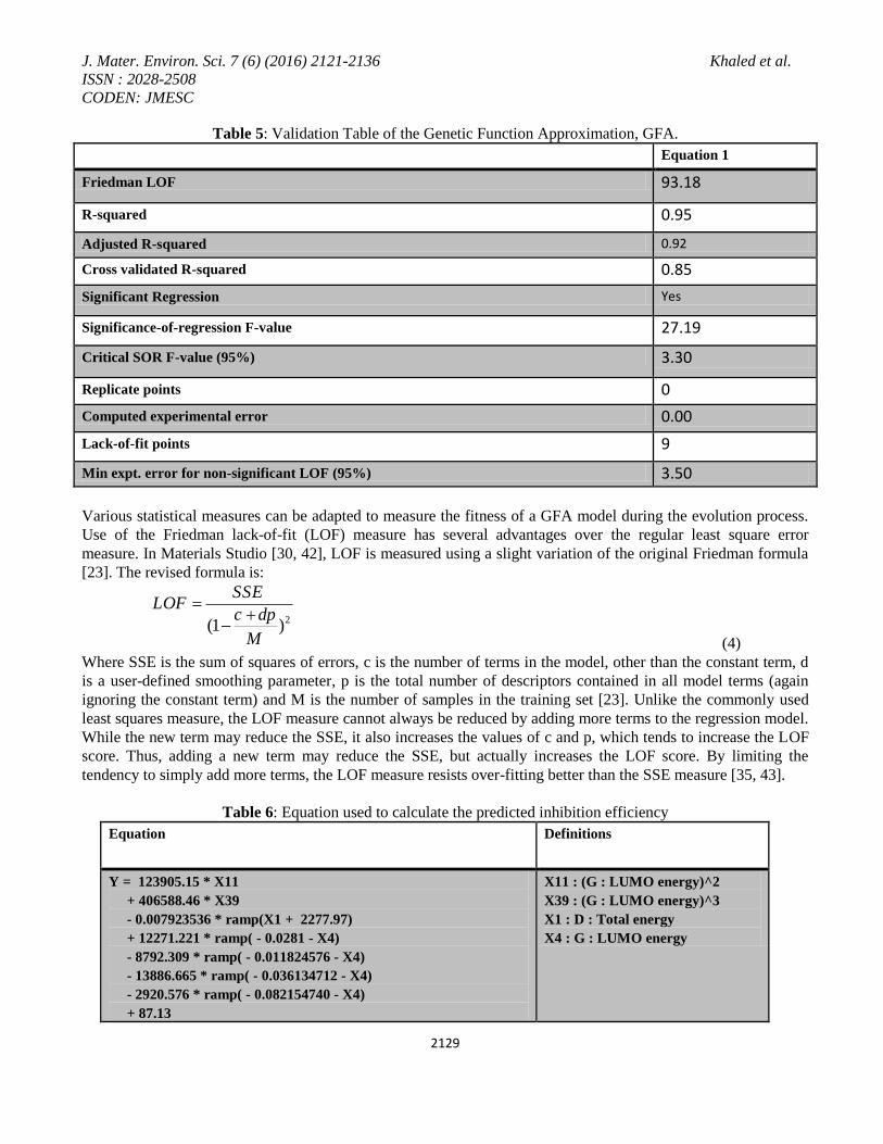
Table 5: Validation Table of the Genetic Function Approximation, GFA.

Equation 1

Friedman LOF 93.18

R-squared 0.95

Adjusted R-squared 0.92

Cross validated R-squared 0.85

Significant Regression Yes

Significance-of-regression F-value 27.19

Critical SOR F-value (95%) 3.30

Replicate points 0

Computed experimental error 0.00

Lack-of-fit points 9

Min expt. error for non-significant LOF (95%) 3.50

Various statistical measures can be adapted to measure the fitness of a GFA model during the evolution process.

Use of the Friedman lack-of-fit (LOF) measure has several advantages over the regular least square error

measure. In Materials Studio [30, 42], LOF is measured using a slight variation of the original Friedman formula

[23]. The revised formula is:

2(1 )

SSELOF

c dp

M

(4)

Where SSE is the sum of squares of errors, c is the number of terms in the model, other than the constant term, d

is a user-defined smoothing parameter, p is the total number of descriptors contained in all model terms (again

ignoring the constant term) and M is the number of samples in the training set [23]. Unlike the commonly used

least squares measure, the LOF measure cannot always be reduced by adding more terms to the regression model.

While the new term may reduce the SSE, it also increases the values of c and p, which tends to increase the LOF

score. Thus, adding a new term may reduce the SSE, but actually increases the LOF score. By limiting the

tendency to simply add more terms, the LOF measure resists over-fitting better than the SSE measure [35, 43].

Table 6: Equation used to calculate the predicted inhibition efficiency

Equation Definitions

Y = 123905.15 * X11

+ 406588.46 * X39

- 0.007923536 * ramp(X1 + 2277.97)

+ 12271.221 * ramp( - 0.0281 - X4)

- 8792.309 * ramp( - 0.011824576 - X4)

- 13886.665 * ramp( - 0.036134712 - X4)

- 2920.576 * ramp( - 0.082154740 - X4)

+ 87.13

X11 : (G : LUMO energy)^2

X39 : (G : LUMO energy)^3

X1 : D : Total energy

X4 : G : LUMO energy


ISSN : 2028-2508

CODEN: JMESC

2130

Table 5 shows the GFA analysis which gives summary of the input parameters used for the calculation. Also, it

reports whether the GFA algorithm converged in specified number of generations. The GFA algorithm is assumed

to have converged when no improvement is seen in the score of the population over a significant length of time,

either that of the best model in each population or the average of all the models in each population. When this

criterion has been satisfied, no further generations are calculated [33].

The Friedman's lack-of-fit (LOF) score in Table 5 evaluates the QSAR model [33]. The lower the LOF, the less

likely it is that GFA model will fit the data. The significant regression is given by F-test, and the higher the value,

the better the model.

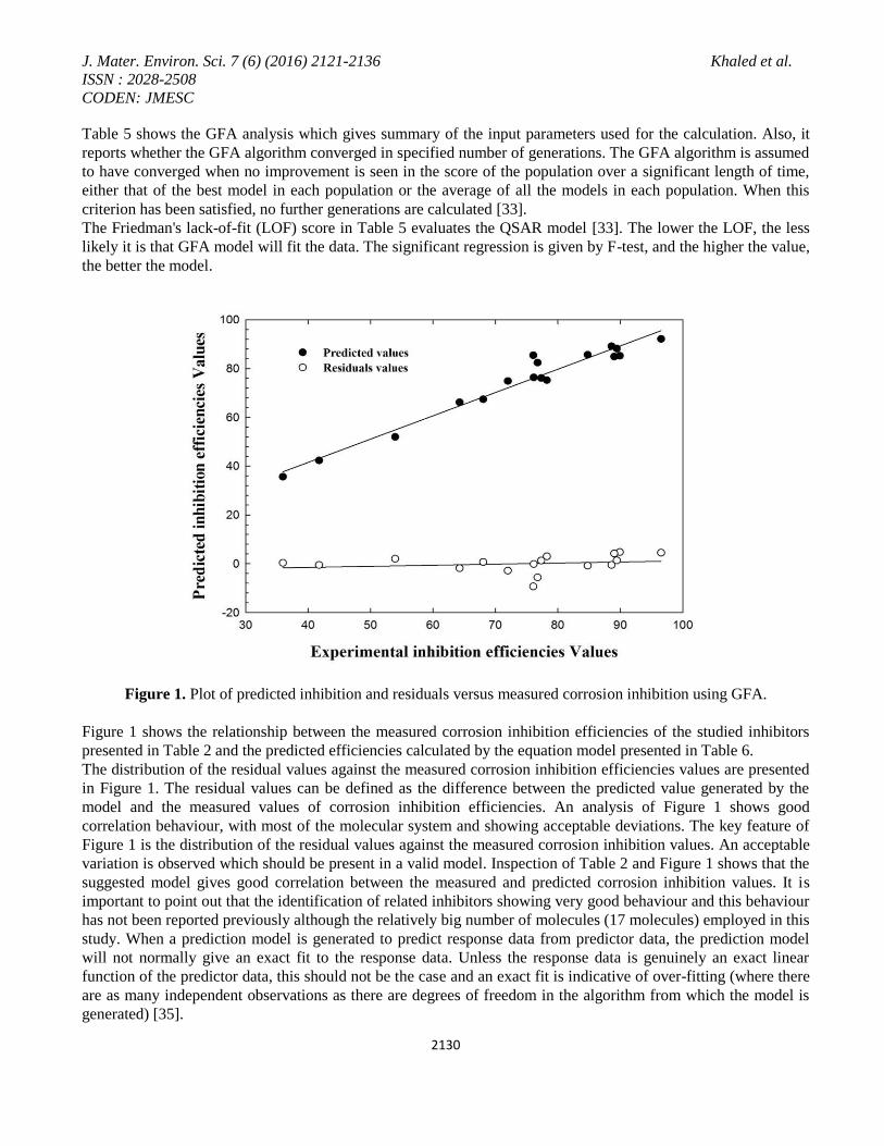
Figure 1. Plot of predicted inhibition and residuals versus measured corrosion inhibition using GFA.

Figure 1 shows the relationship between the measured corrosion inhibition efficiencies of the studied inhibitors

presented in Table 2 and the predicted efficiencies calculated by the equation model presented in Table 6.

The distribution of the residual values against the measured corrosion inhibition efficiencies values are presented

in Figure 1. The residual values can be defined as the difference between the predicted value generated by the

model and the measured values of corrosion inhibition efficiencies. An analysis of Figure 1 shows good

correlation behaviour, with most of the molecular system and showing acceptable deviations. The key feature of

Figure 1 is the distribution of the residual values against the measured corrosion inhibition values. An acceptable

variation is observed which should be present in a valid model. Inspection of Table 2 and Figure 1 shows that the

suggested model gives good correlation between the measured and predicted corrosion inhibition values. It is

important to point out that the identification of related inhibitors showing very good behaviour and this behaviour

has not been reported previously although the relatively big number of molecules (17 molecules) employed in this

study. When a prediction model is generated to predict response data from predictor data, the prediction model

will not normally give an exact fit to the response data. Unless the response data is genuinely an exact linear

function of the predictor data, this should not be the case and an exact fit is indicative of over-fitting (where there

are as many independent observations as there are degrees of freedom in the algorithm from which the model is

generated) [35].


ISSN : 2028-2508

CODEN: JMESC

2131

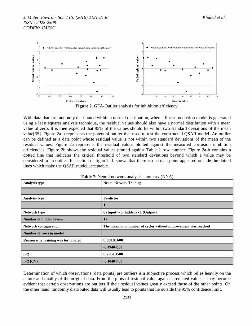
Figure 2. GFA-Outlier analysis for inhibition efficiency.

With data that are randomly distributed within a normal distribution, when a linear prediction model is generated

using a least squares analysis technique, the residual values should also have a normal distribution with a mean

value of zero. It is then expected that 95% of the values should lie within two standard deviations of the mean

value[35]. Figure 2a-b represents the potential outlier that used to test the constructed QSAR model. An outlier

can be defined as a data point whose residual value is not within two standard deviations of the mean of the

residual values. Figure 2a represents the residual values plotted against the measured corrosion inhibition

efficiencies. Figure 2b shows the residual values plotted against Table 2 row number. Figure 2a-b contains a

dotted line that indicates the critical threshold of two standard deviations beyond which a value may be

considered to an outlier. Inspection of figure2a-b shows that there is one data point appeared outside the dotted

lines which make the QSAR model acceptable.

Table 7: Neural network analysis summary (NNA)

Analysis type Neural Network Training

Analysis type Predictor

1

Network type 6 (Input) - 3 (hidden) - 1 (Output)

Number of hidden layers 17

Network configuration The maximum number of cycles without improvement was reached

Number of rows in model

Reason why training was terminated 0.99181600

-0.49404500

r^2 0.70513500

r^2 (CV) -0.10404400

Determination of which observations (data points) are outliers is a subjective process which relies heavily on the

nature and quality of the original data. From the plots of residual value against predicted value, it may become

evident that certain observations are outliers if their residual values greatly exceed those of the other points. On

the other hand, randomly distributed data will usually lead to points that lie outside the 95% confidence limit.


ISSN : 2028-2508

CODEN: JMESC

2132

4.2 Neural Network Analysis

The cross validation data for the neural network model operates by repeating the calculation several times using

subset of the original data to obtain a prediction model and then comparing the predicted values with the actual

values for the omitted data [36]. The main measure of the predictive ability of the model is the correlation

coefficient r2. The closer the value is to 1.0 the better the predictive power. For a good model r

2 value should be

fairly close to 1.0. The correlation coefficient r2 for this study is equal to 0.999 (Table 7) which is reasonably high

that indicates the predictive power of the model.

Investigation of the neural network analysis in QSAR study shows that the network has too many degrees of

freedom (usually the number of network connections between nodes) for the number of observations (rows of

data) for which the network is being trained. In this study there are 6 input, three hidden layers and one output,

summary of the neural network analysis presented in Table 7.

Applying the neural network prediction model generates a model containing predictions corresponding to each

output of the neural network. The neural network model adds a new column containing a calculation of the model

to the study table (Table 2). Also, residual values of the predictions corresponding to each output of the neural

network.

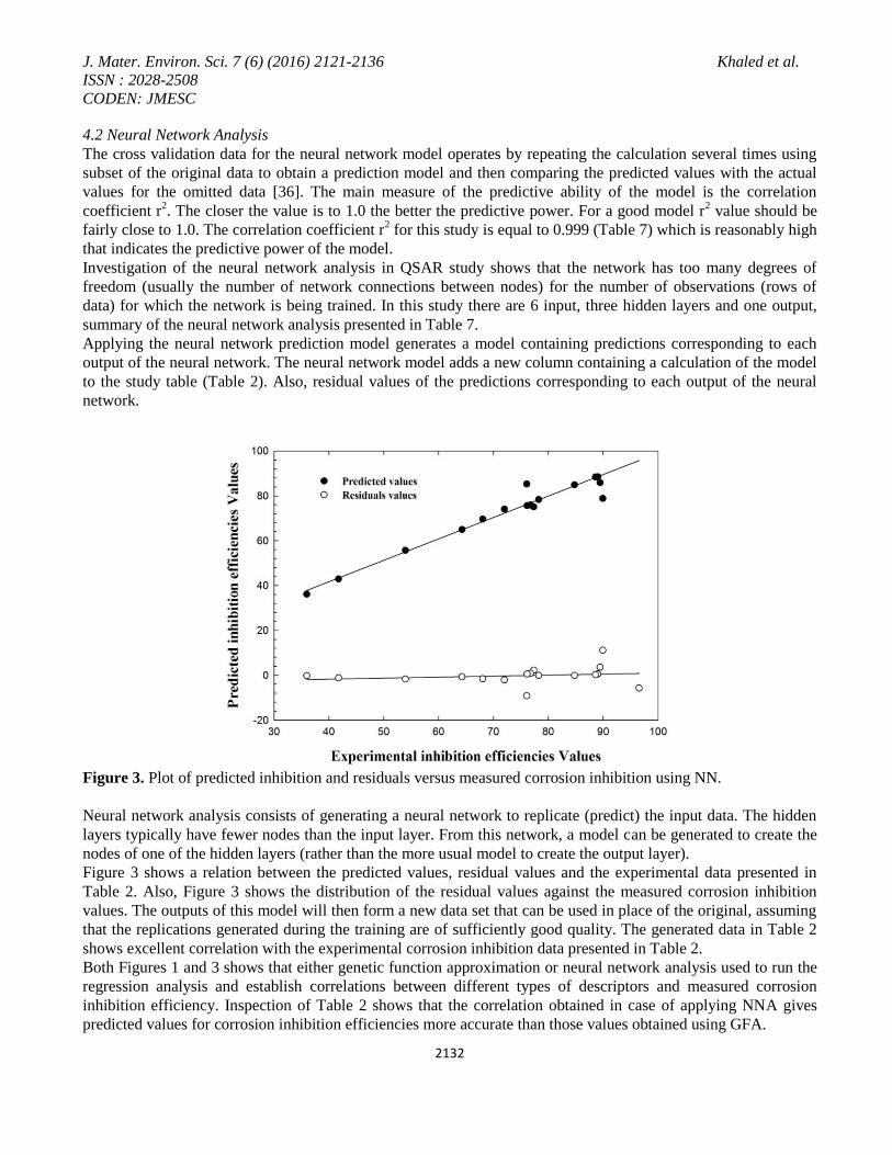
Figure 3. Plot of predicted inhibition and residuals versus measured corrosion inhibition using NN.

Neural network analysis consists of generating a neural network to replicate (predict) the input data. The hidden

layers typically have fewer nodes than the input layer. From this network, a model can be generated to create the

nodes of one of the hidden layers (rather than the more usual model to create the output layer).

Figure 3 shows a relation between the predicted values, residual values and the experimental data presented in

Table 2. Also, Figure 3 shows the distribution of the residual values against the measured corrosion inhibition

values. The outputs of this model will then form a new data set that can be used in place of the original, assuming

that the replications generated during the training are of sufficiently good quality. The generated data in Table 2

shows excellent correlation with the experimental corrosion inhibition data presented in Table 2.

Both Figures 1 and 3 shows that either genetic function approximation or neural network analysis used to run the

regression analysis and establish correlations between different types of descriptors and measured corrosion

inhibition efficiency. Inspection of Table 2 shows that the correlation obtained in case of applying NNA gives

predicted values for corrosion inhibition efficiencies more accurate than those values obtained using GFA.


ISSN : 2028-2508

CODEN: JMESC

2133

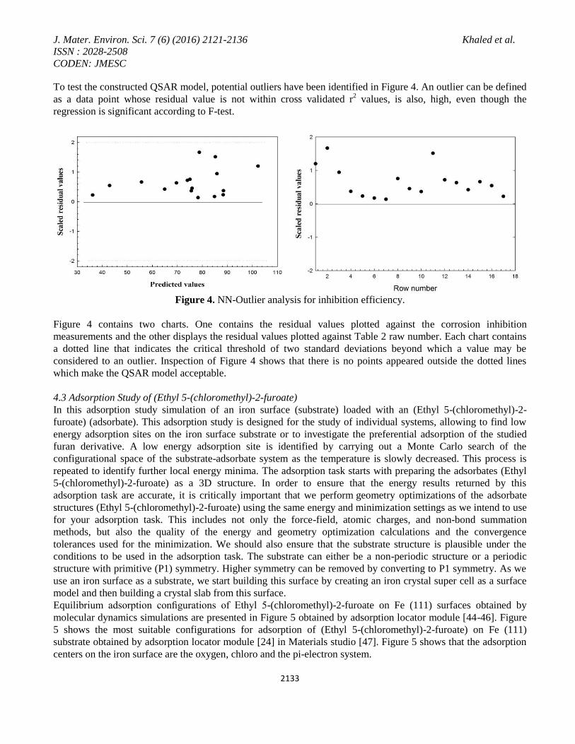
To test the constructed QSAR model, potential outliers have been identified in Figure 4. An outlier can be defined

as a data point whose residual value is not within cross validated r2 values, is also, high, even though the

regression is significant according to F-test.

Figure 4. NN-Outlier analysis for inhibition efficiency.

Figure 4 contains two charts. One contains the residual values plotted against the corrosion inhibition

measurements and the other displays the residual values plotted against Table 2 raw number. Each chart contains

a dotted line that indicates the critical threshold of two standard deviations beyond which a value may be

considered to an outlier. Inspection of Figure 4 shows that there is no points appeared outside the dotted lines

which make the QSAR model acceptable.

4.3 Adsorption Study of (Ethyl 5-(chloromethyl)-2-furoate)

In this adsorption study simulation of an iron surface (substrate) loaded with an (Ethyl 5-(chloromethyl)-2-

furoate) (adsorbate). This adsorption study is designed for the study of individual systems, allowing to find low

energy adsorption sites on the iron surface substrate or to investigate the preferential adsorption of the studied

furan derivative. A low energy adsorption site is identified by carrying out a Monte Carlo search of the

configurational space of the substrate-adsorbate system as the temperature is slowly decreased. This process is

repeated to identify further local energy minima. The adsorption task starts with preparing the adsorbates (Ethyl

5-(chloromethyl)-2-furoate) as a 3D structure. In order to ensure that the energy results returned by this

adsorption task are accurate, it is critically important that we perform geometry optimizations of the adsorbate

structures (Ethyl 5-(chloromethyl)-2-furoate) using the same energy and minimization settings as we intend to use

for your adsorption task. This includes not only the force-field, atomic charges, and non-bond summation

methods, but also the quality of the energy and geometry optimization calculations and the convergence

tolerances used for the minimization. We should also ensure that the substrate structure is plausible under the

conditions to be used in the adsorption task. The substrate can either be a non-periodic structure or a periodic

structure with primitive (P1) symmetry. Higher symmetry can be removed by converting to P1 symmetry. As we

use an iron surface as a substrate, we start building this surface by creating an iron crystal super cell as a surface

model and then building a crystal slab from this surface.

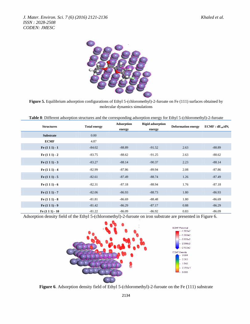
Equilibrium adsorption configurations of Ethyl 5-(chloromethyl)-2-furoate on Fe (111) surfaces obtained by

molecular dynamics simulations are presented in Figure 5 obtained by adsorption locator module [44-46]. Figure

5 shows the most suitable configurations for adsorption of (Ethyl 5-(chloromethyl)-2-furoate) on Fe (111)

substrate obtained by adsorption locator module [24] in Materials studio [47]. Figure 5 shows that the adsorption

centers on the iron surface are the oxygen, chloro and the pi-electron system.


ISSN : 2028-2508

CODEN: JMESC

2134

Figure 5. Equilibrium adsorption configurations of Ethyl 5-(chloromethyl)-2-furoate on Fe (111) surfaces obtained by

molecular dynamics simulations

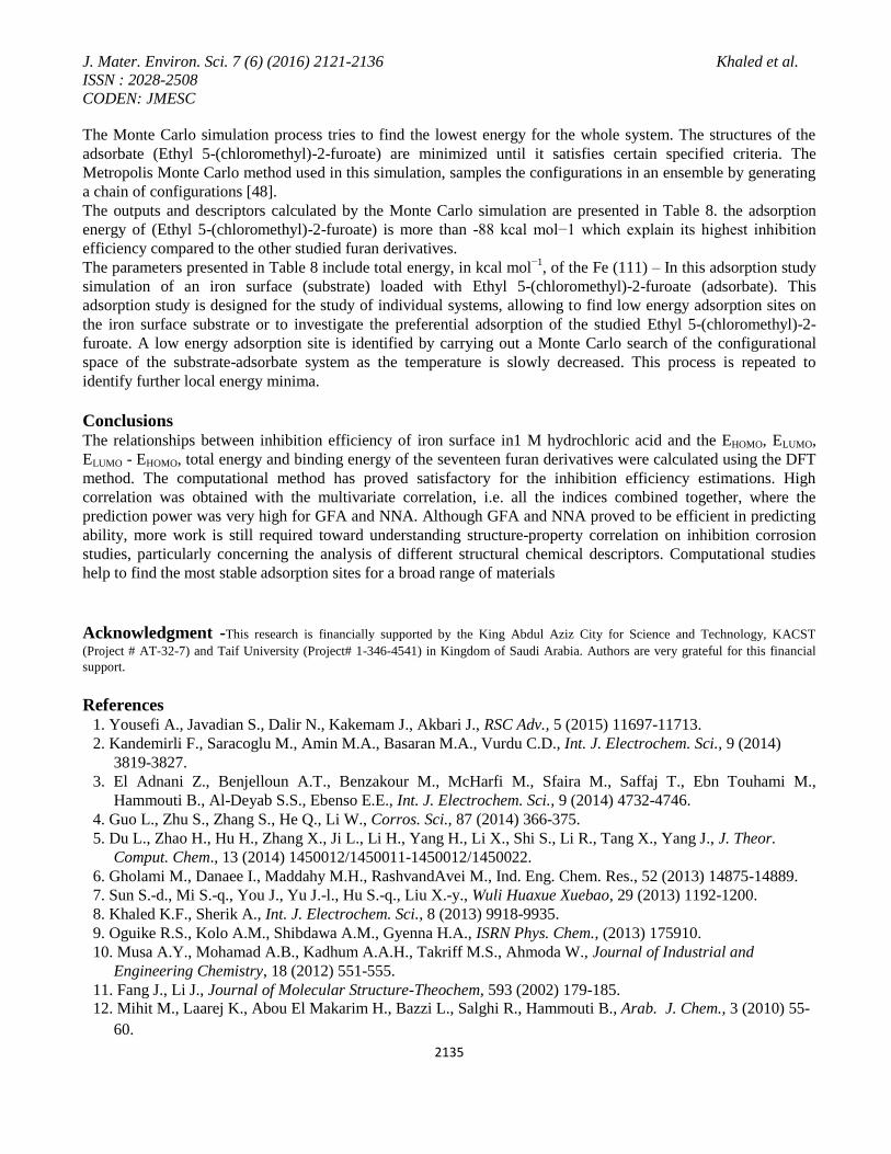
Table 8: Different adsorption structures and the corresponding adsorption energy for Ethyl 5-(chloromethyl)-2-furoate

Structures Total energy Adsorption

energy

Rigid adsorption

energy Deformation energy ECMF : dEad/dNi

Substrate 0.00

ECMF 4.87

Fe (1 1 1) - 1 -84.02 -88.89 -91.52 2.63 -88.89

Fe (1 1 1) - 2 -83.75 -88.62 -91.25 2.63 -88.62

Fe (1 1 1) - 3 -83.27 -88.14 -90.37 2.23 -88.14

Fe (1 1 1) - 4 -82.99 -87.86 -89.94 2.08 -87.86

Fe (1 1 1) - 5 -82.61 -87.49 -88.74 1.26 -87.49

Fe (1 1 1) - 6 -82.31 -87.18 -88.94 1.76 -87.18

Fe (1 1 1) - 7 -82.06 -86.93 -88.73 1.80 -86.93

Fe (1 1 1) - 8 -81.81 -86.69 -88.48 1.80 -86.69

Fe (1 1 1) - 9 -81.42 -86.29 -87.17 0.88 -86.29

Fe (1 1 1) - 10 -81.22 -86.09 -86.92 0.83 -86.09

Adsorption density field of the Ethyl 5-(chloromethyl)-2-furoate on iron substrate are presented in Figure 6.

Figure 6. Adsorption density field of Ethyl 5-(chloromethyl)-2-furoate on the Fe (111) substrate


ISSN : 2028-2508

CODEN: JMESC

2135

The Monte Carlo simulation process tries to find the lowest energy for the whole system. The structures of the

adsorbate (Ethyl 5-(chloromethyl)-2-furoate) are minimized until it satisfies certain specified criteria. The

Metropolis Monte Carlo method used in this simulation, samples the configurations in an ensemble by generating

a chain of configurations [48].

The outputs and descriptors calculated by the Monte Carlo simulation are presented in Table 8. the adsorption

energy of (Ethyl 5-(chloromethyl)-2-furoate) is more than -88 kcal mol−1 which explain its highest inhibition

efficiency compared to the other studied furan derivatives.

The parameters presented in Table 8 include total energy, in kcal mol−1

, of the Fe (111) – In this adsorption study

simulation of an iron surface (substrate) loaded with Ethyl 5-(chloromethyl)-2-furoate (adsorbate). This

adsorption study is designed for the study of individual systems, allowing to find low energy adsorption sites on

the iron surface substrate or to investigate the preferential adsorption of the studied Ethyl 5-(chloromethyl)-2-

furoate. A low energy adsorption site is identified by carrying out a Monte Carlo search of the configurational

space of the substrate-adsorbate system as the temperature is slowly decreased. This process is repeated to

identify further local energy minima.

Conclusions The relationships between inhibition efficiency of iron surface in1 M hydrochloric acid and the EHOMO, ELUMO,

ELUMO - EHOMO, total energy and binding energy of the seventeen furan derivatives were calculated using the DFT

method. The computational method has proved satisfactory for the inhibition efficiency estimations. High

correlation was obtained with the multivariate correlation, i.e. all the indices combined together, where the

prediction power was very high for GFA and NNA. Although GFA and NNA proved to be efficient in predicting

ability, more work is still required toward understanding structure-property correlation on inhibition corrosion

studies, particularly concerning the analysis of different structural chemical descriptors. Computational studies

help to find the most stable adsorption sites for a broad range of materials

Acknowledgment -This research is financially supported by the King Abdul Aziz City for Science and Technology, KACST

(Project # AT-32-7) and Taif University (Project# 1-346-4541) in Kingdom of Saudi Arabia. Authors are very grateful for this financial

support.

References 1. Yousefi A., Javadian S., Dalir N., Kakemam J., Akbari J., RSC Adv., 5 (2015) 11697-11713.

2. Kandemirli F., Saracoglu M., Amin M.A., Basaran M.A., Vurdu C.D., Int. J. Electrochem. Sci., 9 (2014)

3819-3827.

3. El Adnani Z., Benjelloun A.T., Benzakour M., McHarfi M., Sfaira M., Saffaj T., Ebn Touhami M.,

Hammouti B., Al-Deyab S.S., Ebenso E.E., Int. J. Electrochem. Sci., 9 (2014) 4732-4746.

4. Guo L., Zhu S., Zhang S., He Q., Li W., Corros. Sci., 87 (2014) 366-375.

5. Du L., Zhao H., Hu H., Zhang X., Ji L., Li H., Yang H., Li X., Shi S., Li R., Tang X., Yang J., J. Theor.

Comput. Chem., 13 (2014) 1450012/1450011-1450012/1450022.

6. Gholami M., Danaee I., Maddahy M.H., RashvandAvei M., Ind. Eng. Chem. Res., 52 (2013) 14875-14889.

7. Sun S.-d., Mi S.-q., You J., Yu J.-l., Hu S.-q., Liu X.-y., Wuli Huaxue Xuebao, 29 (2013) 1192-1200.

8. Khaled K.F., Sherik A., Int. J. Electrochem. Sci., 8 (2013) 9918-9935.

9. Oguike R.S., Kolo A.M., Shibdawa A.M., Gyenna H.A., ISRN Phys. Chem., (2013) 175910.

10. Musa A.Y., Mohamad A.B., Kadhum A.A.H., Takriff M.S., Ahmoda W., Journal of Industrial and

Engineering Chemistry, 18 (2012) 551-555.

11. Fang J., Li J., Journal of Molecular Structure-Theochem, 593 (2002) 179-185.

12. Mihit M., Laarej K., Abou El Makarim H., Bazzi L., Salghi R., Hammouti B., Arab. J. Chem., 3 (2010) 55-

60.


ISSN : 2028-2508

CODEN: JMESC

2136

13. Behpour M., Ghoreishi S.M., Soltani N., Salavati-Niasari M., Hamadanian M., Gandomi A., Corros. Sci., 50

(2008) 2172-2181.

14. Al Hamzi A.H., Zarrok H., Zarrouk A., Salghi R., Hammouti B., Al-Deyab S.S., Bouachrine M., Amine A.,

Guenoun F., Int. J. Electrochem. Sci., 8 (2013) 2586-2605.

15. John S., Ali K.M., Joseph A., Bull. Mater. Sci., 34 (2011) 1245-1256.

16. Li W., He Q., Pei C., Hou B., Electrochim. Acta, 52 (2007) 6386-6394.

17. Feng L., Yang H., Wang F., Electrochim. Acta, 58 (2011) 427-436.

18. Costa J.M., Lluch J.M., Corros. Sci., 24 (1984) 929-933.

19. Abdul-Ahad P.G., Al-Madfai S.H.F., Corrosion, 45 (1989) 978-980.

20. K.F K., Corros. Sci., 53 (2011) 3457-3465.

21. Rogers D., Hopfinger A.J., J. Chem. Inf. Comput. Sci., 34 (1994) 854-866.

22. Patel H.C., Koehler M., Hopfinger A.J., Am. Chem. Soc., 1995, pp. ENVR-100.

23. Friedman J.H., Multivariate Adaptive Regression Splines, Technical Report No. 102, Laboratory for

Computational Statistics, Department of Statistics, Stanford University, Stanford 1988.

24. Khaled K.F., Al-Mobarak N.A., Int. J. Electrochem. Sci., 7 (2012) 1045-1059.

25. Jahanbani H., El-shafie A.H., Paddy and Water Environment, 9 (2011) 207-220.

26. Wu X., Shi J., Chen F., Wang Y., Kybernetes, 38 (2009) 1684-1692.

27. Dopazo J., Carazo J.M., Journal of Molecular Evolution, 44 (1997) 226-233.

28. Khaled K., Abdel-Shafi N., Int. J. Electrochem. Sci, 6 (2011) 4077-4094.

29. Khaled K.F., J. Solid State Electrochem., 13 (2009) 1743-1756.

30. Delley B., J. Chem. Phys., 92 (1990) 508.

31. Barriga J., Coto B., Fernandez B., Tribology International, 40 (2007) 960-966.

32. Khaled K., Fadl-Allah S.A., Hammouti B., Mater. Chem. Phys., 117 (2009) 148-155.

33. Khaled K.F., Corros. Sci., 53 (2011) 3457-3465.

34. Anonymous, Health & Beauty Close - Up, (2011).

35. Materials Studio 6.0 Manual, Accelrys, (2009).

36. Al-Fakih A.M., Aziz M., Abdallah H.H., Algamal Z.Y., Lee M.H., Maarof H., Int. J. Electrochem. Sci., 10

(2015) 3568-3583.

37. Putz M.V., Putz A.-M., Lazea M., Ienciu L., Chiriac A., International journal of molecular science, 10

(2009) 1193-1214.

38. Steiger J.H., Schonemann P.H., A history of factor indeterminacy. In Theory Construction and Data

Analysis in the Behavioural Science, San Francisco, CA, USA, 1978.1978.

39. Spearman C., The Abilities of Man, MacMillan, London, UK, , 1927.

40. Topliss J.G., Costello R.J., J. Med. Chem., 15 (1972) 1066-1068.

41. Topliss J.G., Edwards R.P., J. Med. Chem., 22 (1979) 1238-1244.

42. Delley B., J. Chem. Phys., 113 (2000) 7756.

43. Accelrys, Inc, Dun and Bradstreet, Inc., Austin, United States, Austin, 2012, pp. 105038.

44. Tamura H., Corros. Sci., 50 (2008) 1872-1883.

45. Tang J., Shao Y., Zhang T., Meng G., Wang F., Corros. Sci., 53 (2011) 1715-1723.

46. Gudze M.T., Melchers R.E., Corros. Sci., 50 (2008) 3296-3307.

47. Delley B., Journal of chemical physics, 92 (1990) 508-517.

48. Accelrys, Materials Studio Manual, Accelrys, USA, 2013.

(2016) ; http://www.jmaterenvironsci.com/

http://www.jmaterenvironsci.com/

QSAR of corrosion inhibitors by genetic function ... · QSAR of corrosion inhibitors by genetic...

Documents

Transcript of QSAR of corrosion inhibitors by genetic function ... · QSAR of corrosion inhibitors by genetic...