Three-dimensional numerical simulation of the dynamic interaction between high-speed trains and a steel-truss arch bridge

*Qing Zeng1), Elias G. Dimitrakopoulos2) and Cheuk Him LO3)

1), 2), 3) Department of Civil and Environmental Engineering, Hong Kong University of

Science and Technology, Clear Water Bay, Kowloon, Hong Kong 1) qzeng@ust.hk

ABSTRACT

The present paper studies the dynamic interaction between high-speed trains and a steel-truss arch bridge with the proposed vehicle-bridge interaction (VBI) model. The train vehicle is treated as a 3D multibody assembly, consisting of one car body, two bogies and four wheelsets. The bridge is simulated with the finite element method (FEM). Particularly, the bridge deck is modeled with shell elements. The contact forces between wheels and rails are derived based on a kinematical constraint on the acceleration level. Key feature of the proposed scheme is the matrix character of the formulation, which results in a set of condensed equations of motion for the VBI system. Track irregularities and wind loading are taken as the excitation to the VBI system. 1. INTRODUCTION To meet the increasing economic and social demands for safer and more efficient transportation, an increased number of high-speed railways (HSR’s) have been built throughout the world, and especially in China. Compared with the conventional railway lines, HSR’s utilize a higher percentage of bridges (Xia, Zhang et al. 2012), mainly for reasons of preventing track settlements and reducing interruptions by surroundings. As a reference, 1059 km of the Beijing-Shanghai HSR line (1318 km long) is on (244) bridges, accounting for a ratio of 80.5%. Among them, the 164 km Danyang-Kunshan Grand Bridge is the longest bridge system in the world (Wikipedia 2015), which is comprised of over 4000 bridge units. In view of the ever increasing number and length of railway bridges, as well as the unprecedented speeds HSR trains operate, the interaction dynamics between (HSR) trains and (railway) bridges should be analyzed in depth to ensure the comfort, and more importantly, the safety of vehicles during the operation. The VBI dynamics attracts the attention of researchers for almost a century (Dimitrakopoulos, Zeng 2015), especially the last decades, due to the advent of high

1) Graduate Student 2) Professor 3) Under Graduate Student

computational power. More sophisticated models, for both bridges and vehicles, are considered. Most recent studies, e.g. (Dimitrakopoulos, Zeng 2015, Antolín, Zhang et al. 2013, Xia, Han et al. 2006, Xu, Zhang et al. 2004, Xia, Xu et al. 2000), simulate the vehicle as a multibody assembly (car-body, bogies and wheelsets), connected with springs and dashpots. As for the bridge model, most of VBI studies focus on simple structural types, e.g. simply supported bridges (Antolín, Zhang et al. 2013), or continuous bridges (Xia, Han et al. 2006). Others consider more sophisticated structural types, such as cable-stayed bridges (Xu, Zhang et al. 2004) or suspension bridges (Xia, Xu et al. 2000). Studies on the dynamic VBI of arch bridges are scarce. Recently, the authors (Dimitrakopoulos, Zeng 2015) proposed a versatile scheme for the dynamic analysis of the VBI system, accounting for different types of bridges and vehicles. Based on the previous work of (Dimitrakopoulos, Zeng 2015), this paper examines the dynamic interaction between HSR train vehicles and a steel arch bridge. The study takes into account the track irregularities and the wind loading excitation. 2. PROPOSED VEHICLE-BRIDGE INTERACTION MODEL The proposed dynamic analysis of the vehicle-bridge interaction (VBI) consists of the vehicle subsystem and the bridge subsystem, together with the track irregularities and the external loading (e.g. wind loading). The two subsystems interact with each other through the contact forces between the vehicle wheels and the rails. The study adopts a global coordinate system for the VBI analysis, and considers the X-axis as the longitudinal direction, the Y-axis the lateral direction, and the Z-axis the vertical direction, following a right-hand rule (Figs 1 and 2). 2.1 Modelling of the vehicle and vehicular dynamics In this study, each vehicle of the train is modeled as a three-dimensional (3D) multibody assembly, consisting of one car body, two bogies and four wheelsets (Fig. 1). The distinct components, the car-body, the bogies and the wheelsets, are rigid bodies connected by linear springs and viscous dashpots, representing the properties of suspension systems. The car-body and the bogies have 5 degrees of freedom (DOF’s) each, and the wheelsets 4 DOF’s each, excluding the pitching DOF (Fig. 1). Therefore, the total DOF’s of each vehicle is 31. The equations of motion (EOM’s) for each vehicle take the form:

,V V V V V V V V VN N T T M u C u K u W λ W λ F (1)

where MV, KV and CV are the mass, stiffness and damping matrices, respectively, of the vehicle given in (Antolín, Zhang et al. 2013). λN and λT are the normal and tangential contact force vectors, respectively (Section 2.3), and V

NW and VTW are

the direction matrices corresponding to λN and λT (Dimitrakopoulos, Zeng 2015). Throughout this paper, the subscripts N and T, denote the normal and the tangential directions of contact, respectively. The only nonzero entries in matrices V

NW and VTW correspond to the wheels of the vehicle. For the upper part of the vehicle, i.e., the

car body and the bogies, the pertinent sub-matrices are zero (Dimitrakopoulos, Zeng

2015). FV is the external force vector of the vehicle, including the weight and the wind loading (when considered).

Fig. 1 Vehicle model: (a) side view, (b) back view, (c) top view, and (d) terminology.

Fig. 2 The examined arch bridge. 2.2 Modelling of the bridge The examined bridge is a steel arch truss bridge for a HSR line. The arch bridge, consists of parabolic arch ribs, main girders, struts, crossbeams, stringers and suspenders, all made of steel, and a bridge deck made of concrete (Fig. 2). The length

Z

X

car-body

wheelset

bogie

(a)

(c)

speed vZ

Y

(b)

(d)

Y (lateral)

Z (vertical)(yawing)

(rolling)XY

terminology

(vertical)

(pitching)

(lateral)

(lateral)(rolling)

(lateral)

(yawing)

λN1 λN2λT1

and the width of the bridge are 140 m and 16 m, respectively. The bridge is modeled with finite elements, considering the complete geometrical model, instead of the modal superposition method. The arch ribs, main girders, struts, crossbeams, and stringers, are modelled with beam elements; the vertical suspenders are modelled with axial-deformed truss elements; the bridge deck is modelled with shell elements. Six DOF’s are considered per node: three translations and three rotations with respect to the X, Y and Z axes accordingly. The stiffness matrix KB , the mass matrix MB and the Rayleigh damping matrix CB (assuming a damping ratio of 0.05 for the first two modes) are obtained from an in-house algorithm, developed and verified, previously (Zeng, Dimitrakopoulos 2015). The EOM’s for the bridge are:

, B B B B B B B B BN N T TM u C u K u W λ W λ F (2)

where uB is the bridge displacement vector and FB is the vector of the loads acting on the bridge, including the wind loading (when considered); B

NW and BTW are the

contact force direction matrices for the bridge, which contain shape functions for the shell elements (Cook 2007). The nonzero entries in the B

NW and BTW matrices

correspond to the DOF’s of the shell elements taking participating in the contact (Dimitrakopoulos, Zeng 2015). 2.3 Modelling of interaction between the two sub-systems The contact forces are the key connecting the two subsystems, i.e. the vehicle (Eq. (1)) and the bridge vehicle (Eq. (2)). Firstly, the pertinent vectors/matrices of the two individual subsystems in Eqs. (1) and (2) are assembled as:

* ,t M u Cu Ku Wλ F (3)

where

, , , , ,

, , , ,

V V V V V

B B B B B

V VN N T

N T N TB BT N T

M K C u FM K C u F

M K C u F

λ W Wλ W W W W W

λ W W

(4)

The calculation of the contact forces adopts a macroscopic “rigid contact” model, assuming no separation in the normal direction and no sliding in the tangential direction, as in (Dimitrakopoulos, Zeng 2015), which is checked for each analysis. Specifically, each wheelset considers two normal contact forces and one tangential contact force (Fig. 1(b)). On the acceleration level, the “rigid contact” states that the relative wheel/ rail acceleration is zero. Finally, the global EOM’s of the VBI system become (Dimitrakopoulos, Zeng 2015):

* * * , t t t t t tMu C u K u F (5)

with

*

*

*

1 1T 1 T

1 1T 1 2 T

1 1T 1 2

2

,

c

t t t t t t t

t t t t t t t

t t t t t t t

v

v

v

E W G W M W G W

E W G W M K W G W

E

C C

K

W G W M F W rF G

(6)

where E is an identity matrix. Matrix G is equal to G = WTM-1W, and its inverse G-1 represents the mass activated by the contact. cr is the track irregularities. Note that

the global stiffness matrix K*(t), the global damping matrix C*(t) and the global loading vector F*(t) of the coupled system are all time-dependent. 3. RESULTS AND DISCUSSION In this study, we first consider, a single vehicle representing the locomotive, and a completed train consisting of ten vehicles, running over the bridge with a speed of v = 300 km/h. Before the vehicle enters the bridge, it is assumed that the vehicle runs on tracks lying on the rigid ground with the same track irregularities as on the bridge, and it has come to an equilibrium configuration with initial non-zero deformation when it enters the bridge. The dynamic VBI starts when the first vehicle enters the bridge and stops when the last vehicle of train leaves the bridge. After a vehicle leaves the bridge, its response is not of concern for this study, similarly to (Dimitrakopoulos, Zeng 2015). The examined point of the bridge is the midpoint of the midspan (Fig. 2). Fig. 3 plots the time-histories of the response of both the bridge and the vehicle. Specifically, Fig. 3 (a) and (b) compares the vertical displacement of the examined point of the bridge, induced by the passage of a single vehicle and ten vehicles, respectively. In the vertical direction, the behavior of the bridge due to the VBI resembles quasi-static loading conditions. In general, the more vehicles are, the larger the vertical displacement of the bridge and the longer “deflection-plateau” are (Fig. 3 (a) and (b)). Besides, the midpoint of the bridge deflects upwards (from 0 to 0.5s in Fig. 3 (a) and (b)), when the vehicles are running on the first half span of the bridge. Therefore, the vertical displacement of the bridge resembles the deformation pattern of a beam supported on continuous springs. The maximum vertical displacement of the bridge is around 3 mm, well within the requirement from the code, e.g. 1/800 of the span, (China's Ministry of Railways 2009), indicating the high stiffness of the bridge in the vertical direction. Further, Fig. 3 (c) to (e) investigate the response of the first vehicle, considering ten vehicles passing over the bridge. Fig. 3 (c) plots the normal contact force of the wheel 1 (λN1 in Fig. 1) of the first vehicle. λN1 vibrates about the value of the static weight of a specific wheel (71.12 kN), due to the presence of track irregularities. The vertical acceleration of the first vehicle (Fig. 3 (d)) is well below the contemporary code limit for HSR e.g. (China's Ministry of Railways 2009): 1.2 m/s2. Fig. 3 (e) plots the vertical displacement of the car-body of the first vehicle. The displacement of the vehicle starts with non-zero deformation when it enters the bridge (-0.388 m), due to the weight of the vehicle. As the bridge deflects by the moving vehicles, it affects in turn the response of the vehicles; the car-body of the vehicle

defects downwards, following the trend of the downward deformation of the bridge. Two peak values appear in Fig. 3 (e), corresponding to the two bogies of the specific vehicle (Fig. 1).

Fig. 3 The vertical displacement time-histories of the bridge, induced by the passage of (a) a single vehicle and (b) ten vehicles; (c) the normal contact force of wheel 1, (d) the

vertical acceleration and (e) the vertical displacement of the first vehicle. Fig. 4 plots the deformed shape of the bridge for six different time instants, which correspond to different numbers of vehicles running on the bridge. For the visualization of the results, and not for the analysis of the response, we employ again the commercially available software ANSYS (ANSYS 2011). The bridge displays different

0 0.5 1 1.5 2 2.5 3 3.5 4 4.5 5-4

-3

-2

-1

0

1

0 0.5 1 1.5 265

70

75

80

0 0.5 1 1.5 2-4

-3

-2

-1

0

1

0 0.5 1 1.5 2-0.2

-0.1

0

0.1

0.2

(a)

● u: displacement ● a: acceleration ● λN: normal contact force ● NV: vehicle number

u

BZ (

mm

)

(b)

uB

Z (

mm

)

a

VZ

1 (m

/s2 )

time (s) time (s)

(d)

car-body of 1st vehicle

λ N

1 (k

N)

(c)

with the passage of 10 vehicles

wheel 1 of

the 1st vehicle

0 0.5 1 1.5 2-0.394

-0.392

-0.39

-0.388

-0.386

u

VZ

1 (m

)

(e)

car-body of 1st vehicle

with the passage of 1 vehicle

71.12 kN

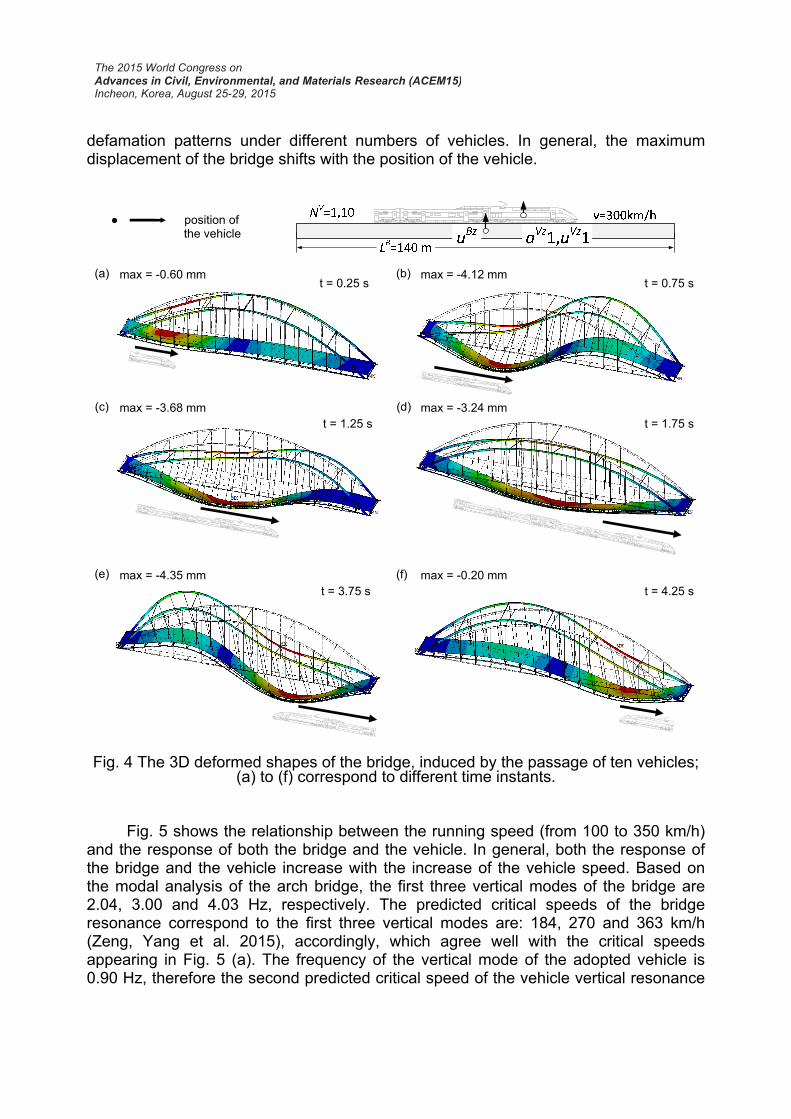
defamation patterns under different numbers of vehicles. In general, the maximum displacement of the bridge shifts with the position of the vehicle.

Fig. 4 The 3D deformed shapes of the bridge, induced by the passage of ten vehicles; (a) to (f) correspond to different time instants.

Fig. 5 shows the relationship between the running speed (from 100 to 350 km/h) and the response of both the bridge and the vehicle. In general, both the response of the bridge and the vehicle increase with the increase of the vehicle speed. Based on the modal analysis of the arch bridge, the first three vertical modes of the bridge are 2.04, 3.00 and 4.03 Hz, respectively. The predicted critical speeds of the bridge resonance correspond to the first three vertical modes are: 184, 270 and 363 km/h (Zeng, Yang et al. 2015), accordingly, which agree well with the critical speeds appearing in Fig. 5 (a). The frequency of the vertical mode of the adopted vehicle is 0.90 Hz, therefore the second predicted critical speed of the vehicle vertical resonance

t = 0.25 s

t = 1.25 s t = 1.75 s

t = 4.25 st = 3.75 s

t = 0.75 s

max = -4.35 mm

max = -3.68 mm

max = -0.20 mm

max = -3.24 mm

max = -0.60 mm (a)

(c)

(e)

(b)

(d)

(f)

● position of the vehicle

max = -4.12 mm

is 227 km/h (Zeng, Yang et al. 2015). The numerical critical speed from the VBI analysis (Fig. 5 (b)) is in good agreement with predicted critical speed. The pertinent acceleration is amplified in the vicinity of the resonance speed (Fig. 5 (b)).

Fig. 5 The (a) vertical displacement of the bridge and (b) the acceleration of the first vehicle, vs. vehicle speed.

Fig. 6 extends the work of Fig. 3, accounting for the wind loading on both the bridge and the vehicle. The study considers three values of wind velocity: 0 (i.e. no wind), 10 and 30 m/s. The wind flow direction is assumed constantly along the lateral direction (Y-axis) of the bridge. The simulation of the time-domain fluctuating wind velocity adopts the spectral representation method (Cao, Xiang et al. 2000). The wind loading on the bridge consists of the steady-state forces due to the mean wind velocity, and the buffeting forces due to the fluctuating wind velocity. The self-excited forces, due to the intense vibration of the bridge itself, are considered negligible because of the high stiffness of this particular bridge (Guo, Xia et al. 2011). Due to lack of wind tunnel test to obtain the aerodynamic parameters for this particular bridge, the drag (lateral), lift (vertical), and moment (rolling) coefficients of the bridge are assumed as 1.18, 0.12 and 0.21, and their first derivatives are 0.00, 0.00 and 3.70, respectively, when the attack angle of wind is zero (Xu, Zhang et al. 2004). The wind loading on the vehicle considers the steady-state forces due to the mean wind velocity. The drag (lateral), lift (vertical), and moment (rolling) aerodynamic parameters of the train vehicle are 0.30, 0.25 and 0.30, respectively (Xu, Zhang et al. 2004). The wind loading lifts up the bridge structure; therefore, the larger the wind velocity is, the smaller the vertical displacement of the bridge is (Fig. 6 (a)). Without wind, the lateral displacement of the bridge starts with zero value and vibrates about the undeformed geometry (Fig. 6 (b)). The presence of the wind forces the bridge to deform laterally and the pertinent time history starts with a non-zero value and vibrates about the deformed geometry (Fig. 6 (b)). The larger wind velocity results in a larger lateral displacement of the bridge, as it is expected. Regarding the response of the

100 150 200 250 300 3500.06

0.08

0.1

0.12

0.14

0.16

● u: displacement ● a: acceleration ● λN: normal contact force ● NV: vehicle number

uB

Z (

mm

)

vehicle speed (v) vehicle speed (v)

(a)

aV

Z1

(m/s

2 )

(b)

car-body of 1st vehicle

100 150 200 250 300 350

2.9

3.05

3.1

3.15

190 km/h

350 km/h

280 km/h

225 km/h

vehicle, the vertical acceleration of the vehicle is not significantly affected by wind loading (Fig. 6 (c)). The present of the wind loading amplifies the lateral acceleration of the vehicle. The pertinent lateral acceleration increases with increase of the wind velocity (Fig. 6 (d)). More significantly, the two important metrics of the safety of the running vehicle, the derailment factor and the offload factor, are amplified due to the wind loading, from 0.06 and 0.01 (without wind) to 0.37, 0.40 (Uw = 10 m/s), 0.45 and 0.44 (Uw = 30 m/s). The pertinent thresholds are 0.8 and 0.6 (China's Ministry of Railways 2009); therefore for the examined wind loading case, the safety of the vehicle is guaranteed.

Fig. 6 The (a) vertical and the (b) lateral displacement time-histories of the bridge; the (c) vertical and the (d) lateral acceleration of the vehicle, induced by the passage of ten

vehicles and wind loading. 4. CONCLUSIONS This study examines a realistic vehicle-bridge interaction case, focusing on the HSR vehicles and a steel arch bridge. The study considers different loading cases, including: the passage of a single locomotive and a completed train consisting of ten vehicles; different running speeds of the vehicles and different wind velocities.

0 0.5 1 1.5 2 2.5-0.2

-0.1

0

0.1

0.2

0.3

● u: displacement ● a: acceleration ● λN: normal contact force ● NV: vehicle number

uBZ (

mm

)

time (s) time (s)

(a)

uBY (

mm

)

(b)

car-body of 1st vehicle

0 1 2 3 4 5-0.1

0

0.1

0.2

0.3

0.4

0.5

0 0.5 1 1.5 2 2.5-0.2

-0.1

0

0.1

0.2

0 1 2 3 4 5-4

-3

-2

-1

0

1

aV

Z (

m/s

2 )

(c)

a

VY (

m/s

2 )

(c)

Uw = 30 m/s

Uw = 0 (no wind)

Uw = 10 m/s

car-body of 1st vehicle

LB=140 m

NV=10 v=300km/huBz

uBy

aVz1aVy1

The results show that the arch bridge has good dynamic properties to ensure a safe and comfort running of the train vehicles, without other external loading, e.g. wind loading. For the considered wind loading, larger wind velocity results in larger lateral displacement of the bridge and larger lateral acceleration of the vehicle, but smaller vertical displacement of the bridge. The presence of the wind load reduces the running safety of the vehicles. However, the present study offers only a glimpse into the complex and multi-parametric vehicle-bridge interaction problem under wind loading, and further extensive parametric studies are needed to reach conclusions of general value. REFERENCES ANSYS. (2011), ANSYS User's Manual Version 14.0. Houston, USA: ANSYS Inc. ANTOLÍN, P., ZHANG, N., GOICOLEAA, J.M., XIA, H., ASTIZA, M.Á and OLIVAA, J.

(2013), “Consideration of nonlinear wheel-rail contact forces for dynamic vehicle-bridge interaction in high-speed railways,” J. Sound Vibrat., 332, 1231-1251.

CAO, Y., XIANG, H. and ZHOU, Y. (2000), “Simulation of stochastic wind velocity field on long-span bridges,” J. Eng. Mech., 126(1), 1-6.

CHINA'S MINISTRY OF RAILWAYS. (2009), “Code for Design of High Speed Railway”. COOK, R.D., 2007. “Concepts and applications of finite element analysis,” New York:

Wiley. DIMITRAKOPOULOS, E.G. and ZENG, Q. (2015). “A three-dimensional dynamic

analysis scheme for the interaction between trains and curved railway bridges,” Comput. Struct., 149, 43-60.

GUO, WW., XIA, H., ZHANG, T. and SUN, G. (2011), “Dynamic responses of a railway bridge under high-speed trains subjected to turbulent winds”, Proceedings of the 8th International Conference on Structural Dynamics (EURODYN 2011), 1164-1171.

WIKIPEDIA, 2015-last update, Danyang-Kunshan Grand Bridge. Available: http://en.wikipedia.org/wiki/Danyang\%E2\%80\%93Kunshan\_Grand\_Bridge [02/06, 2015].

XIA, H., XU, Y.L. and CHAN, T. (2000), “Dynamic interaction of long suspension bridges with running trains,” J. Sound. Vibrat., 237(2), 263-280.

XIA, H., ZHANG, N. and GUO, W. (2012), “Application of train-bridge-interaction analysis to bridge design of high-speed railways in China”, Proceedings of the 1st International Workshop on High-Speed and Intercity Railways, Springer, 355-371.

XIA, H., HAN, Y., ZHANG, N. and GUO, W. (2006), “Dynamic analysis of train–bridge system subjected to non‐uniform seismic excitations,” Earthquake Eng. Struct. Dyn., 35(12), 1563-1579.

XU, Y., ZHANG, N. and XIA, H. (2004), “Vibration of coupled train and cable-stayed bridge systems in cross winds,” Eng. Struct., 26(10), 1389-1406.

ZENG, Q. and DIMITRAKOPOULOS, E.G. (2015), “Seismic response analysis of an interacting curved bridge-train system under frequent earthquakes,” Earthquake Eng, Struct. Dyn. (under consideration)

ZENG, Q., YANG, Y.B. and DIMITRAKOPOULOS, E.G., 2015. “Dynamic response of high speed vehicles and sustaining curved bridges under conditions of resonance,” Eng. Struct. (under consideration)