Q D U STANDING PART INFORMATION IN CNNS

Under review as a conference paper at ICLR 2020

QUANTITATIVELY DISENTANGLING AND UNDER-STANDING PART INFORMATION IN CNNS

Anonymous authorsPaper under double-blind review

ABSTRACT

This paper presents an unsupervised method to learn a neural network, namely anexplainer, to disentangle and quantify the knowledge of object parts that is usedfor inference by a pre-trained convolutional neural network (CNN). The explain-er performs like an auto-encoder, which quantitatively disentangles part featuresfrom intermediate layers and uses the part features to reconstruct CNN featureswithout much loss of information. The disentanglement and quantification of partinformation help people understand intermediate-layer features used by the CNN.More crucially, we learn the explainer via knowledge distillation without usingany annotations of object parts or textures for supervision. In experiments, ourmethod was widely used to diagnose features of different benchmark CNNs, andexplainers significantly boosted the feature interpretability.

1 INTRODUCTION

Convolutional neural networks (CNNs) (LeCun et al., 1998; Krizhevsky et al., 2012; He et al., 2016)have shown promise in many visual tasks, but the model interpretability has been an Achilles’ heelof deep neural networks for decades. Especially in recent years, helping CNNs to earn trust forsafety issues in critical applications has become a new demand for CNNs beyond the accuracy.

Therefore, in order to explain the knowledge contained in a CNN, we aim to quantify signals inintermediate-layer features, which represent object objects, away from signals for other concepts(e.g. textures). Note that as shown in Table 1, our objective is not to qualitatively visualize object-part features within a CNN. Instead, this work quantitatively explains how much information ofobject parts and how much information of other concepts are used by the CNN for prediction. Thequantitative disentanglement of object-part information and other concepts from an intermediatelayer can provide new insights of information processing inside the CNN, and is of considerabletheoretical values in explainable AI.

Crucially, we are not given any manual annotations of object parts in this study. Bau et al. (2017)used annotations of object parts2, textures and other visual concepts to quantify the semantic mean-ing of each filter. However, the requirement for the rigorous analysis of part concepts conflicts withthe fact that there does exist comprehensive annotations of all object parts and textures. It is be-cause object parts encoded by the CNN usually do not have explicit names (e.g. the combinationof the neck and the left shoulder), thereby difficult to be annotated. In comparison, we propose toobjectively quantify the ratio of object-part concepts to all other concepts (see Table 3), which is notsupposed not to be affected by the potential subjective bias in human annotations.

Therefore, potential issues in above tasks can be summarized as follows.

• Automatic disentanglement of explainable1 (object-part) information and unexplainable informa-tion that are activated in an intermediate layer is necessary for a rigorous and trustworthy diagnosisof CNNs. Each filter of a conv-layer usually encodes a mixture of various semantics and noises (seeFig. 1).

2In (Zhang et al., 2018c), both “objects” and “parts” are categorized as parts.1In this study, we do not distinguish the subtle difference between terms of interpretable and explainable.

We use terms of interpretable conv-layers and interpretable filters as defined in (Zhang et al., 2018c).

1


… ... APerformer

Explainer

BEncoder Decoder

Filter 1

Filter 2

Unclear semantics

Unclear semantics

Filter 1

Filter 2

Head pattern

Torso pattern

Feature maps of ordinary filters Feature maps of interpretable filters

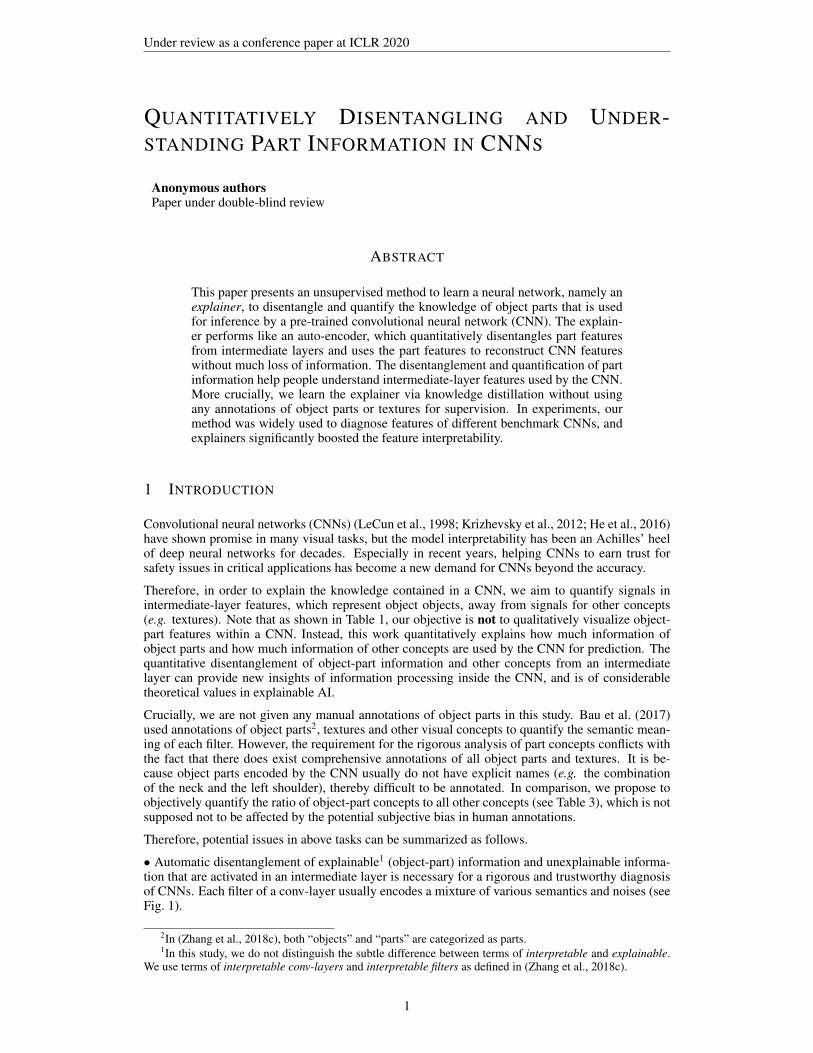
Figure 1: Explainer network. We use an explainer network to disentangle object-part features thatused by a pre-trained performer network. The explainer network disentangles object-part features(B) from the performer to mimic signal processing in the performer. The explainer network can alsoinvert the disentangled object-part features to reconstruct features of the performer without muchloss of information. We compare traditional features (A) in the performer and the disentangledfeatures (B) in the explainer on the right. The gray and green lines indicate the information-passroute during the inference process and that during the diagnosis process, respectively.

Traditional CNNs Interpretable CNNs (Zhang et al., 2018c) Capsule nets (Sabour et al., 2017) Visualization & diagnosis ExplainerCan explain pre-trained model X XDisentangle explainable signals X X XSemantic-level explanation X X XHigh feature interpretability X X — XHigh discrimination power X Do not affect the pre-trained modelPotential broad applicability X X X

Table 1: Comparison between our research and other studies. Note that this table can only summa-rize mainstreams in different research directions considering the huge research diversity. Please seeSection 2 for detailed discussions of related work.

Therefore, the disentanglement of object-part information requires us 1. to mathematically modeland distinguish features corresponding to object parts away from textures and noises, without anypart annotations; and 2. to quantify neural activations for object parts and other concepts. Forexample, 90% signals for inference may be quantified as object parts and treat the rest 10% may beconsidered as textures and noises.

• Semantic explanations: Furthermore, the disentangled features can be assigned with different ob-ject parts with clear semantic meanings. In comparisons, network visualization and diagnosis (Fong& Vedaldi, 2017; Selvaraju et al., 2017; Ribeiro et al., 2016; Lundberg & Lee, 2017) mainly illus-trate the appearance corresponding to a network output/filter at the pixel level, without quantitativelysummarizing strict semantics. Our method identifies which object parts are used for inference. Com-pared to previous pixel-level visualization and diagnosis of a CNN, our quantitative disentanglementof object-part features presents a more trustworthy way to diagnose CNNs.

Tasks, learning networks to diagnose networks: We propose a new strategy to boost feature inter-pretability. Given a pre-trained CNN, we learn another neural network, namely a explainer network,to transform and decompose chaotic intermediate-layer features of the CNN into (1) elementaryfeatures corresponding to object parts and (2) unexplainable features. Accordingly, the pre-trainedCNN is termed a performer network.

As shown in Fig. 1, the performer is trained for superior performance, in which each filter usuallyrepresents a chaotic mixture of object parts and textures (Bau et al., 2017). The explainer workslike an auto-encoder, which is learned to mimic the logic of the performer. Two specific sets offilters in the explainer decomposes performer features into features of object parts and other con-cepts, respectively. Then, the decomposed features are also trained to reconstruct features of upperlayers of the performer. The explainer is attached onto the performer without affecting the originaldiscrimination power of the performer.

A high reconstruction quality ensures the explainer successfully mimics the signal processing inthe performer (please see Appendix C for more discussions). Besides, the disentangled object-partfeatures can be treated as a paraphrase of performer feature representations. The proposed methodroughly quantifies the ratio of neural activations for object parts, i.e. telling us• how much features (e.g. 90%) in the performer can be explained as object parts;• information of what parts is encoded in the performer;• for each specific inference score, which object parts activate filters in the performer, and how muchthey contribute to the inference.

Diagnosing black-box networks vs. learning interpretable1 networks: As compared in Table 1,diagnosing pre-trained black-box neural networks has distinctive contributions beyond learning se-mantically meaningful intermediate-layer features, such as (Sabour et al., 2017; Zhang et al., 2018c).It is because traditional black-box networks have exhibited much broader applicability than inter-

2


p

1-pConv-ordin ReLU Norm Pool

Conv-interp-2

ReLU

Mask

LossfConv-interp-1

ReLU

Mask

Lossf Norm

Pool

ReLU

FC

-

dec-1

FC

-

dec-2

Reconstruction loss

Reconstruction loss

Interpretabletrack

Ordinarytrack D

ecoder

Encode

r

Performer

p

1-p

Interpretable Track

Ordinary Track

Encode

r Decoder

Performer

Conv-

ordin

ReLU

Norm

Pool

Conv-interp-2

ReLU

Mask

LossfConv-interp-1

ReLU

Mask

Lossf Norm

Pool

Ordinary track

Interpretabletrack

DecoderReLUfc-dec-1 fc-dec-2

Reconstruction loss

Reconstruction loss

Mask

Conv-interp-1

ReLU

Lossf Mask

Conv-interp-2

ReLU

Lossf Norm

Pool

Conv-ordin

ReLU

Norm

Pool

Interpretable track

Ordinary track Decoder

ReLU fc-dec-2fc-dec-1

Interpretable Track

Ordinary Track

p

1-p

Decoder

… ...Performer

Explaine

rFigure 2: The explainer network (left). Detailed structures within the interpretable1 track, the ordi-nary track, and the decoder are shown on the right. People can change the number of conv-layersand FC layers within the encoder and the decoder for their own applications.

pretable networks.• Model flexibility: Most existing CNNs are black-box models with low interpretability, so diagnos-ing pre-trained CNNs has broad applicability. In comparison, interpretable neural networks usuallyhave specific requirements for structures (Sabour et al., 2017) or losses (Zhang et al., 2018c), whichlimit the model flexibility and applicability.• Interpretability vs. discriminability: Unlike diagnosing pre-trained networks, learning inter-pretable networks usually suffers from the dilemma between the feature interpretability and itsdiscrimination power. A high interpretability is not equivalent to, and sometimes conflicts witha high discrimination power. As shown in (Sabour et al., 2017), increasing the interpretability of aneural network may affect its discrimination power. Furthermore, filter losses in the interpretableCNN (Zhang et al., 2018c) greatly hurts the classification performance when the network has so-phisticated structures (please see Appendix A). People usually have to trade off between the networkinterpretability and the performance in real applications.

Learning: We learn the explainer by distilling feature representations from the performer to theexplainer. No annotations of parts or textures are used to guide the feature disentanglement duringthe learning process. We add a loss to specific filters in the explainer (see Fig. 2). Without partannotations, the filter loss automatically encourages the filter to be exclusively triggered by a certainobject part of a category. This filter is termed an interpretable1 filter.

Meanwhile, the disentangled object-part features are also required to reconstruct features of upperlayers of the performer. Successful feature reconstructions guarantee to avoid significant informationloss during the disentanglement of part features.

Contributions of this study are summarized as follows.• We tackle a new strategy to diagnose pre-trained neural networks, i.e. learning an explainer net-work to disentangle object-part concepts that are used by a pre-trained CNN. Our method roughlyquantifies neural activations corresponding to object parts, which sheds new light on understandingblack-box models.• Our method is able to learn the explainer without any annotations of object parts or texturesfor supervision. Experiments show that our approach has considerably improved the feature inter-pretability.

2 RELATED WORK

Network interpretability: Instead of analyzing network features from a global view (Wolchover,2017; Schwartz-Ziv & Tishby, 2017; Rauber et al., 2016), (Bau et al., 2017) defined six kinds ofsemantics for intermediate-layer feature maps of a CNN, i.e. objects, parts, scenes, textures, mate-rials, and colors. Fong and Vedaldi (Fong & Vedaldi, 2018) analyzed how multiple filters jointlyrepresented a certain semantic concept. We can roughly consider the first two semantics as objectparts with explicit shapes, and summarize the last four semantics as textures. Our research aims todisentangle object-part information from intermediate layers of the performer network.

Many studies for network interpretability mainly showed visual appearance corresponding to a neu-ral unit inside a CNN (Zeiler & Fergus, 2014; Mahendran & Vedaldi, 2015; Simonyan et al., 2013;Dosovitskiy & Brox, 2016; Yosinski et al., 2015; Dong et al., 2017) or extracted image regions thatwere responsible for network output (Ribeiro et al., 2016; Elenberg et al., 2017; Koh & Liang, 2017;Fong & Vedaldi, 2017; Selvaraju et al., 2017; Kumar et al., 2017). Other studies retrieved mid-levelrepresentations with specific meanings from CNNs for various applications (Kolouri et al., 2017;

3


Lengerich et al., 2017). For example, (Zhou et al., 2015; 2016) selected neural units to describe“scenes”. (Simon & Rodner, 2015) discovered objects from feature maps of unlabeled images. Infact, each filter in an intermediate conv-layer usually encodes a mixture of parts and textures, andthese studies consider the most notable part/texture component as the semantic meaning of a fil-ter. In contrast, our research uses a filter loss to purify the semantic meaning of each filter (Fig. 1visualizes the difference between the two types of filters).

A new trend related to network interpretability is to learn networks with disentangled, explainablerepresentations (Hu et al., 2016; Stone et al., 2017; Liao et al., 2016). Many studies learn explainablerepresentations in a weakly-supervised or unsupervised manner. For example, capsule nets (Sabouret al., 2017) and interpretable RCNN (Wu et al., 2017) learned interpretable intermediate-layer fea-tures. InfoGAN (Chen et al., 2016) and β-VAE (Higgins et al., 2017) learned meaningful inputcodes of generative networks. The study of interpretable CNNs (Zhang et al., 2018c) developed aloss to push each intermediate-layer filter towards the representation of a specific object part duringthe learning process without given part annotations. However, as mentioned in (Bau et al., 2017), aninterpretable model cannot always ensure a high discrimination power, which limits the applicabilityof interpretable models. Therefore, instead of directly boosting the interpretability of the performernetwork, we propose to learn an explainer network in an unsupervised fashion. (Vaughan et al.,2018) distilled knowledge of a network into an additive model, but this study does not explain thenetwork at a semantic level.

Meta-learning: Our study is also related to meta-learning (Chen et al., 2017; Andrychowicz et al.,2016; Li & Malik, 2016; Wang et al., 2017). Meta-learning uses an additional model to guide thelearning of the target model. In contrast, our research uses an additional explainer network to explainintermediate-layer features of the target performer network.

3 ALGORITHM

3.1 NETWORK STRUCTURE OF THE EXPLAINER

As shown in Fig. 2, the explainer network has two modules, i.e. an encoder and a decoder, which de-compose the performer’s intermediate-layer features into explainable object-part features and invertobject-part features back to features of the performer, respectively. If features of the performer canbe well reconstructed, then we can roughly consider that the decomposed features contain nearly thesame information as features in the performer.

We applied the encoder and decoder with following structures to all types of performers in experi-ments. Nevertheless, people can change the layer number of the explainer in their applications.

Encoder: In order to reduce the risk of over-interpreting textures or noises as parts, we design twotracks for the encoder, namely an interpretable1 track with interpretable filters and an ordinary trackwith ordinary filters, which model object-part features and other features, respectively. Although asdiscussed in (Zhang et al., 2018c), a high conv-layer mainly represents parts rather than textures,avoiding over-interpreting is still necessary for the explainer.

The interpretable track disentangles object parts from chaotic features. This track has two inter-pretable conv-layers (namely conv-interp-1,conv-interp-2), each followed by a ReLU layer and amask layer. The interpretable conv-layer is defined in (Zhang et al., 2018c). Each filter in an in-terpretable conv-layer is learned to be exclusively triggered by a specific object part, and is termedan interpretable filter. This interpretable filter is learned using both the task loss and an filter loss.The filter loss boosts the interpretability, which will be introduced later. Besides, the ordinary trackcontains a conv-layer (namely conv-ordin), a ReLU layer, and a pooling layer.

We sum up output features of the interpretable track xinterp and those of the ordinary track xordin as thefinal output of the encoder, i.e. xenc = p · xinterp + (1− p) · xordin, where a scalar weight p measures thequantitative contribution from the interpretable track. p is parameterized as a sigmoid probabilityp = sigmoid(wp), wp ∈ θ, where θ is the set of parameters to be learned. Our method encourages alarge p so that most information in xenc comes from the interpretable track.

For example, if p = 0.9, we can roughly consider that about 90% feature information from theperformer can be represented as object parts due to the use of norm-layers.

4


Norm-layer: We normalize xinterp and xordin to make the probability p accurately represent the ratioof the contribution from the interpretable track, i.e. making each channel of these feature mapsproduces the same magnitude of activation values. Thus, we add two norm-layers to the interpretabletrack and the ordinary track (see Fig. 2). For each input feature map x ∈ RL×L×D, the normalizationoperation is given as x(ijk) = x(ijk)/αk, where αk ∈ α ⊂ θ denotes the average activation magnitudeof the k-th channel αk = Ex[

∑ij max(x(ijk), 0)] through feature maps of all images, where x(ijk)

denotes an element in x. We update α during the forward propagation, just like in the learning forbatch normalization.

Mask layer: We add mask layers after two interpretable conv-layers to remove activations that areunrelated to the target part. As shown in Fig. 3, each activated feature map after the mask layeralways has a single activation peak.

Let xf ∈ RL×L denote the feature map of an interpretable filter f after the ReLU operation. Themask layer localizes the potential target object part on xf as the neural unit with the strongestactivation µ = argmaxµ=[i,j]x

(ij)f , where µ=[i, j] denotes a neural unit in xf (1≤ i, j≤L), and x(ij)f

indicates its activation value.

Based on the estimated part location µ, the mask layer assigns xf with a mask maskf to removenoises, xmasked

f = xf ◦maskf , where ◦ denotes the Hadamard product. The mask w.r.t. µ is given asmaskf = max(Tµ, 0), where Tµ is a pre-define template with a single activation peak at µ. Theo-retically, there are various choices for the template shape, but for simplicity, we used part templatesin (Zhang et al., 2018c) in this study, i.e. T (ij)

µ = max{1 − 4‖µ−[i,j]‖1L , 0}. ‖ · ‖1 denotes the L-1

norm. Given µ, we treat maskf as a constant to enable gradient back-propagation.

Decoder: The decoder inverts xenc to xdec to reconstruct performer features. The decoder has two FClayers, namely fc-dec-1 and fc-dec-2, which are used to reconstruct feature maps of two correspond-ing FC layers in the performer. The reconstruction loss will be introduced later. The better featurereconstruction indicates that the explainer’s feature xenc loses less information.

3.2 LEARNING

When we distill knowledge representations from the performer to the explainer, we minimize thefollowing loss for each input image.

Loss(θ)=∑l∈L

λ(l)‖x(l)−x∗(l)‖2−η log p+∑f

λf ·Lossf (xf ) (1)

where θ denotes the set of parameters to be learned, including filter weights of conv-layers andFC layers in the explainer, wp for p, and parameters for norm-layers. λ(l), λf and η are scalarhyper-parameters.

• The first term ‖x(l)−x∗(l)‖2 is the reconstruction loss, which also minimizes the information losswhen we use the explainer’s features to mimic the logic of the performer. x(l) denotes the featureof the FC layer l in the decoder, L = {fc − dec − 1, fc − dec − 2}. x∗(l) indicates the correspondingfeature in the performer.

• The second term − log p encourages the interpretable track to make more contribution to theinference. In other words, this term forces object-part information in the performer’s features gothrough the interpretable track, instead of going through the traditional track a short-cut path.

• The third term Lossf (xf ) is the loss of filter interpretability. Without annotations of object parts,the filter loss forces each filter xf to be exclusively triggered by a specific object part of a certaincategory.

During the back propagation, the interpretable filter f receives gradients from both the filter loss andthe reconstruction loss to update its weights. Whereas, ordinary filters in the ordinary track and thedecoder only learn from gradients of the reconstruction loss.

The filter loss was formulated in (Zhang et al., 2019) as the minus mutual information between thedistribution of feature maps and that of part locations. Given an input image, xf is learned to satisfythat if the target part appears, then xf should have a single activation peak at the part location;otherwise, xf should keep inactivated.

Lossf =∑

xf∈XLossf (xf ) = −MI(X;P) = −

∑µ∈P

p(µ)∑

xf∈Xp(xf |µ) log

p(xf |µ)p(xf )

(2)

5


where MI(·) indicates the mutual information. X denotes a set of feature maps of the filter f , whichare extracted from different input images. P = {µ|µ = [i, j], 1 ≤ i, j ≤ L} ∪ {∅} is referred to asa set of all part-location candidates. As mentioned above, each location µ = [i, j] is referred to asan activation unit in the feature map. Besides, ∅ ∈ P denotes the case that the target part of thefilter does not appear in the input image, and we expect all units in xf to keep inactivated. The jointprobability p(xf , µ) describes the compatibility between xf and µ. Please see (Zhang et al., 2018c)or Appendix H for details of p(µ) and p(xf |µ). The filter loss ensures xf match only one of allL2 + 1 location candidates.

As shown in Fig. 2, we add a filter loss to each interpretable filter f in the two conv-layers (conv-interp-1 and conv-interp-2). xf ∈ RL×L denotes the feature map of the interpretable filter after theReLU operation.

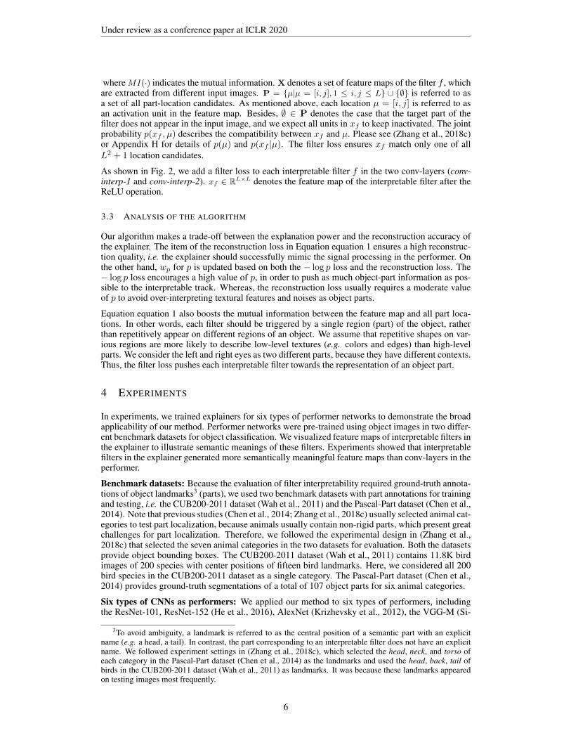
3.3 ANALYSIS OF THE ALGORITHM

Our algorithm makes a trade-off between the explanation power and the reconstruction accuracy ofthe explainer. The item of the reconstruction loss in Equation equation 1 ensures a high reconstruc-tion quality, i.e. the explainer should successfully mimic the signal processing in the performer. Onthe other hand, wp for p is updated based on both the − log p loss and the reconstruction loss. The− log p loss encourages a high value of p, in order to push as much object-part information as pos-sible to the interpretable track. Whereas, the reconstruction loss usually requires a moderate valueof p to avoid over-interpreting textural features and noises as object parts.

Equation equation 1 also boosts the mutual information between the feature map and all part loca-tions. In other words, each filter should be triggered by a single region (part) of the object, ratherthan repetitively appear on different regions of an object. We assume that repetitive shapes on var-ious regions are more likely to describe low-level textures (e.g. colors and edges) than high-levelparts. We consider the left and right eyes as two different parts, because they have different contexts.Thus, the filter loss pushes each interpretable filter towards the representation of an object part.

4 EXPERIMENTS

In experiments, we trained explainers for six types of performer networks to demonstrate the broadapplicability of our method. Performer networks were pre-trained using object images in two differ-ent benchmark datasets for object classification. We visualized feature maps of interpretable filters inthe explainer to illustrate semantic meanings of these filters. Experiments showed that interpretablefilters in the explainer generated more semantically meaningful feature maps than conv-layers in theperformer.

Benchmark datasets: Because the evaluation of filter interpretability required ground-truth annota-tions of object landmarks3 (parts), we used two benchmark datasets with part annotations for trainingand testing, i.e. the CUB200-2011 dataset (Wah et al., 2011) and the Pascal-Part dataset (Chen et al.,2014). Note that previous studies (Chen et al., 2014; Zhang et al., 2018c) usually selected animal cat-egories to test part localization, because animals usually contain non-rigid parts, which present greatchallenges for part localization. Therefore, we followed the experimental design in (Zhang et al.,2018c) that selected the seven animal categories in the two datasets for evaluation. Both the datasetsprovide object bounding boxes. The CUB200-2011 dataset (Wah et al., 2011) contains 11.8K birdimages of 200 species with center positions of fifteen bird landmarks. Here, we considered all 200bird species in the CUB200-2011 dataset as a single category. The Pascal-Part dataset (Chen et al.,2014) provides ground-truth segmentations of a total of 107 object parts for six animal categories.

Six types of CNNs as performers: We applied our method to six types of performers, includingthe ResNet-101, ResNet-152 (He et al., 2016), AlexNet (Krizhevsky et al., 2012), the VGG-M (Si-

3To avoid ambiguity, a landmark is referred to as the central position of a semantic part with an explicitname (e.g. a head, a tail). In contrast, the part corresponding to an interpretable filter does not have an explicitname. We followed experiment settings in (Zhang et al., 2018c), which selected the head, neck, and torso ofeach category in the Pascal-Part dataset (Chen et al., 2014) as the landmarks and used the head, back, tail ofbirds in the CUB200-2011 dataset (Wah et al., 2011) as landmarks. It was because these landmarks appearedon testing images most frequently.

6


Feature maps of an interpretable filter in

the explainerFeature maps of an ordinary filter in the

performer



performer



performer

Figure 3: Visualization of interpretable filters in the explainer and ordinary filters in the performer.As discussed in (Bau et al., 2017), the top conv-layer of a CNN is more likely to represent objectparts than low conv-layers. We compared filters in the top conv-layer of the performer and inter-pretable filters in the conv-interp-2 layer of the explainer. We used (Zhou et al., 2015) to visualizethe RF4 of neural activations in a feature map after a ReLU layer and a mask layer. Ordinary filtersare usually activated by repetitive textures, while interpretable filters always represent the same partthrough different images, which are more semantically meaningful. Please see Appendix B for moreresults.

monyan & Zisserman, 2015), the VGG-S (Simonyan & Zisserman, 2015), the VGG-16 (Simonyan& Zisserman, 2015).

Two experiments: We followed experimental settings in (Zhang et al., 2018c) to conduct two ex-periments, i.e. an experiment of single-category classification and an experiment of multi-categoryclassification. For single-category classification, we trained six performers with structures of theAlexNet (Krizhevsky et al., 2012), VGG-M (Simonyan & Zisserman, 2015), VGG-S (Simonyan& Zisserman, 2015), VGG-16 (Simonyan & Zisserman, 2015), ResNet-101 (He et al., 2016), andResNet-152 (He et al., 2016) for the seven animal categories in the two benchmark datasets. Thus,we trained 40 performers, each of which was learned to classify objects of a certain category fromother objects. We cropped objects of the target category based on their bounding boxes as posi-tive samples. Images of other categories were regarded as negative samples. For multi-categoryclassification, we trained the VGG-M (Simonyan & Zisserman, 2015), VGG-S (Simonyan & Zis-serman, 2015), and VGG-16 (Simonyan & Zisserman, 2015) to classify the six animal categories inthe Pascal-Part dataset (Chen et al., 2014).

Experimental details: As discussed in (Bau et al., 2017), high conv-layers in a CNN (performer)are more likely to represent object parts, while low conv-layers mainly encode textures. Therefore,we used feature maps before the top conv-layer of the performer as the input of the explainer, i.e. therelu4 layer of the AlexNet/VGG-M/VGG-S (the 12th/12th/11th layer of the AlexNet/VGG-M/VGG-S) and the relu5-2 layer of the VGG-16 (the 28th layer). Note that we did not select feature mapsof the top conv-layer to enable a fair comparison, because we can parallel the top conv-layer of theperformer to the conv-ordin layer of the explainer. For ResNets, we used the output feature of thelast residual block as the input of the explainer. We trained the explainer network to disentanglethese feature maps for testing.

For ordinary CNNs, the output of the explainer reconstructed the feature of the fc7 layer of theAlexNet/VGG-M/VGG-S/VGG-16 performer and was fed back to the performer. Thus, a recon-struction loss matched features between the fc-dec-2 layer of the explainer and the fc7 layer of theperformer. Another reconstruction loss connected the fc-dec-1 layer of the explainer and the previ-ous fc6 layer of the performer. For ResNets, feature maps of fc-dec-1 and fc-dec-2 correspond tooutputs of the second last residual block and the last residual block, respectively, although they arenot FC layers. Each conv-layer in the explainer had D filters with a 3×3×D kernel and a biasedterm, where D is the channel number of its input feature map. We used zero padding to ensure theoutput feature map had the same size of the input feature map. The fc-dec-1 and fc-dec-2 layers inthe explainer copied filter weights from the fc6 and fc7 layers of the performer, respectively. Poolinglayers in the explainer were also parameterized according to the last pooling layer in the performer.

7


Single-category Multibird cat cow dog horse sheep Avg. Avg.

AlexNet 0.153 0.131 0.141 0.128 0.145 0.140 0.140 –Explainer 0.104 0.089 0.101 0.083 0.098 0.103 0.096 –VGG-M 0.152 0.132 0.143 0.130 0.145 0.141 0.141 0.135Explainer 0.106 0.088 0.101 0.088 0.097 0.101 0.097 0.097VGG-S 0.152 0.131 0.141 0.128 0.144 0.141 0.139 0.138Explainer 0.110 0.085 0.098 0.085 0.091 0.096 0.094 0.107VGG-16 0.145 0.133 0.146 0.127 0.143 0.143 0.139 0.128Explainer 0.095 0.089 0.097 0.085 0.087 0.089 0.090 0.109ResNet-101 0.147 0.134 0.142 0.127 0.144 0.142 0.139 –Explainer 0.098 0.088 0.099 0.088 0.088 0.093 0.092 –ResNet-152 0.148 0.134 0.143 0.128 0.145 0.142 0.140 –Explainer 0.097 0.088 0.098 0.089 0.088 0.092 0.092 –

Table 2: Location instability of feature maps between per-formers and explainers that were trained using the Pascal-Part dataset (Chen et al., 2014). A low location instabilityindicates a high filter interpretability. Please see Appendix Ffor comparisons with more baselines.

Pascal-Part dataset CUB200Single-class Multi-class dataset

AlexNet – 0.7137 0.5810VGG-M 0.9012 0.8066 0.8611VGG-S 0.9270 0.8996 0.9533VGG-16 0.8593 0.8718 0.9579ResNet-101 0.9727 – –ResNet-152 0.9833 – –

Table 3: Average p values of ex-plainers. p measures the quanti-tative contribution from the inter-pretable track. When we used anexplainer to diagnose feature map-s of a VGG network, about 86%–96% activation scores came fromexplainable features.

We set η = 1.0 × 106 for the AlexNet, VGG-M, and VGG-S, because these three CNNs havesimilar numbers of layers. We set η = 1.5×105 for the VGG-16 and ResNets, since they have moreconv-layers. For each type of CNN performers, the parameter setting was uniformly applied to thelearning of different performers for various categories. We set λ(l) = 5 × 104/Ex∗

(l)[‖max(x∗(l), 0)‖],

where the expectation was averaged over features of all images.

Evaluation metric: We compared the object-part interpretability between feature maps of the ex-plainer and those of the performer. To obtain a convincing evaluation, we both visualized filters (seeFig. 3) and used the objective metric of location instability to measure the fitness between a filter fand the representation of an object part.

The metric of location instability was widely used (Zhang et al., 2018c). As discussed in (Zhanget al., 2018c), compared to the interpretability metric in (Bau et al., 2017), the location instability isa more reasonable metric when the filter is automatically learned without ground-truth annotationsor scales of parts (see Appendix G for details). Given a feature map xf , we localized the part at theunit µ with the highest activation. We used (Zhou et al., 2015) to project the part coordinate µ on thefeature map onto the image plane and obtained pµ. We assumed that if the filter f consistently rep-resented the same object part of a certain category through different images, then distances betweenthe inferred part location pµ and some object landmarks3 of the category should not change a lot a-mong different objects. For example, if f always represented the head part on different objects, thenthe distance between the localized part pµ (i.e. the dog head) and the ground-truth landmark of theshoulder should keep stable, although the head location pµ changes in different images. Thus, forsingle-category classification, we computed the deviation of the distance between pµ and a specificlandmark through objects of the category, and we used the average deviation w.r.t. various land-marks to evaluate the location instability of f . The location instability was reported as the averagedeviation, when we computed deviations using all pairs of filters and landmarks of the category. Formulti-category classification, we first determined the target category of each filter f and then com-puted the location instability based on objects of the target category. We assigned each interpretablefilter in the explainer to the category whose images can activate the filter most. Please see (Zhanget al., 2018c) for computational details of this evaluation metric.

According to network structures used in experiments, we can parallel the explainer to the top conv-layer of the performer, because they both receive features from the relu4/relu5-2 layer of the per-former and output features to the upper layers of the performer. Crucially, as discussed in (Bauet al., 2017), low conv-layers in a CNN usually represent colors and textures, while high conv-layersmainly represent object parts; the top conv-layer of the CNN is most likely to model object partsamong all conv-layers. Therefore, to enable a fair comparison, we compared feature maps of theconv-interp-2 layer of the explainer with feature maps of the top conv-layer of the performer.

4.1 EXPERIMENTAL RESULTS AND ANALYSIS

Tables 2 and 4 compare the interpretability between feature maps in the performer and feature mapsin the explainer. Feature maps in our explainers were much more explainable than feature maps in

8


AlexNet VGG-M VGG-S VGG-16Performer 0.1502 0.1476 0.1481 0.1373Explainer 0.0906 0.0815 0.0704 0.0490

Table 4: Location instability of feature maps in per-formers and explainers that were trained using theCUB200-2011 dataset (Wah et al., 2011). A low lo-cation instability indicates a high filter interpretabili-ty. Please see Appendix F for comparisons with morebaselines.

Performer Explainer ∆ ErrorVGG-M 6.12% 6.62% 0.5%VGG-S 5.95% 6.97% 1.02%VGG-16 2.03% 2.17% 0.14%ResNet-101 1.67% 3.19% 1.52%ResNet-152 0.71% 1.55% 0.84%

Table 5: Multi-category classificationerrors using features of performers andexplainers based on the Pascal-Partdataset (Chen et al., 2014). Please seeAppendix J for more results of performersand explainers.

Filter 1 in the VGG‐16

performer

Filter 2 in the VGG‐16

performer

Filter 1 in the AlexNet

performer

Filter 2 in the AlexNet

performer

activations are disentangled as object parts

activations are disentangled as object parts

Figure 4: Comparisons of feature maps of different performers corresponding to different valuesof p. 95.8% of VGG-16 features were disentangled as object parts, while only 58.1% of AlexNetfeatures were disentangled as object parts. Note that each visualized filter of the performer does notstrictly represent a single object part, which is different from interpretable filters in the explainer.

performers in all comparisons. The explainer exhibited only 35.7%–68.8% of the location instabilityof the performer, which means that interpretable filters in the explainer more consistently describedthe same object part through different images than filters in the performer.

The p value of an explainer indicates the quantitative ratio of the contribution from explainable fea-tures. Table 3 lists p values of explainers that were learned for different performers. p measures thequantitative contribution from the interpretable track. For example, the VGG-16 network learnedusing the CUB200-2011 dataset has a p value p = 0.9579, which means that about 95.8% featureinformation of the performer can be represented as object parts, and only about 4.2% feature in-formation comes from textures and noises. In contrast, the AlexNet is not so powerful in learningobject-part features. Only about 58.1% feature information describes object parts, when the AlexNetis learned the CUB200-2011 dataset.

Fig. 4 visualizes feature maps of the VGG-16 and AlexNet to demonstrate the difference betweendifferent conv-layers in part information. We found that the explainer disentangled more featuresfrom the VGG-16 network as object parts than those from the AlexNet. Accordingly, the visualizedfeature maps of the VGG-16 network were also more localized and more related to part pattern-s. Note that p is just a rough measurement of object-part information. Accurately disentanglingsemantic information from a CNN is still a significant challenge.

To evaluate feature reconstructions of an explainer, we fed the reconstructed features back to theperformer for classification. As shown in Table 5, we compared the classification accuracy of ex-plainer’s reconstructed features with the accuracy based on original performer features. Performersoutperformed explainers in object classification. We used the explainer’s increase of classificationerrors w.r.t. the performer (i.e. “∆ Error” in Table 5) to measure the information loss during featuretransformation in the explainer.

Visualization of filters: We used the visualization method proposed by (Zhou et al., 2015) to com-pute the receptive field (RF) of neural activations of an interpretable filter (after ReLU and maskoperations), which was scaled up to the image resolution. As mentioned in (Zhou et al., 2015),the computed RF represented image regions that were responsible for neural activations of a filter,

9


a head filter

a torso filter

interpretable Ordinary interpretable Ordinary interpretable Ordinary

58 head filters: contributing 12.8%

243 torso filters:contributing 44.8%

167 neck filters:contributing 42.2%

44 other filters:contributing 0.2%

interpretable

Figure 5: Grad-CAM attention maps and quantitative analysis. We used (Selvaraju et al., 2017)to compute grad-CAM attention maps of interpretable feature maps in the explainer and ordinaryfeature maps in the performer. Interpretable filters focused on a few distinct object parts, whileordinary filters separated its attention to both textures and parts. We can assign each interpretablefilter with a semantic part. E.g. the network learned 58, 167, and 243 filters in the conv-interp-2 layerto represent the head, neck, and torso of the bird, respectively. We used the linear model in (Zhanget al., 2018b) to estimate contributions of different filters to the classification score. We summedup contributions of a part’s filters as the part’s quantitative contribution. Please see Appendix D formore results.

which was much smaller than the theoretical size of the RF. Fig. 3 used RFs4 to visualize inter-pretable filters in the conv-interp-2 layer of the explainer and ordinary filters in the top conv-layerof the performer. Fig. 5 compares grad-CAM attention maps (Selvaraju et al., 2017) of the conv-interp-2 layer in the explainer and those of the top conv-layer of the performer. Interpretable filtersin an explainer mainly represented an object part, while feature maps of ordinary filters were usuallyactivated by different image regions without clear meanings.

5 CONCLUSION AND DISCUSSIONS

In this paper, we have proposed a new network-diagnosis strategy, i.e. learning an explainer net-work to disentangle object-part features and other features that are used by a pre-trained performernetwork. We have developed a simple yet effective method to learn the explainer, which guaranteesthe high interpretability of feature maps without using annotations of object parts or textures forsupervision. Theoretically, our explainer-performer structure supports knowledge distillation intonew explainer networks with different losses. People can revise network structures inside the or-dinary track, the interpretable track, and the decoder and apply novel interpretability losses to theinterpretable track.

We divide the encoder of the explainer into an interpretable track and an ordinary track to reduce therisk of over-interpreting textures or noises as parts. Fortunately, experiments have shown that mostof signals in the performer can be explained as parts.

Directly learning interpretable features (Zhang et al., 2018c) may hurt the discrimination power,especially when the CNN has complex structures (e.g. residual networks, see Section 1). In compar-ison, learning an explainer does not affect the performer, thereby ensuring the broad applicability.

We have applied our method to different types of performers, and experimental results show that ourexplainers can disentangle most information in the performer into object-part feature maps, whichsignificantly boosts the feature interpretability. E.g. for explainers for VGG networks, more than80% signals go through the interpretable track, so they can be explained as object-part information.

4When an ordinary filter in the performer does not have consistent contours, it is difficult for (Zhou et al.,2015) to align different images to compute the average RF. Thus, for performers, we simply used a round RFfor each activation. We overlapped all activated RFs in a feature map to compute the final RF.

10


REFERENCES

Marcin Andrychowicz, Misha Denil, Sergio Gomez Colmenarejo, Matthew W. Hoffman, DavidPfau, Tom Schaul, Brendan Shillingford, and Nando de Freitas. Learning to learn by gradientdescent by gradient descent. In NIPS, 2016.

David Bau, Bolei Zhou, Aditya Khosla, Aude Oliva, and Antonio Torralba. Network dissection:Quantifying interpretability of deep visual representations. In CVPR, 2017.

X. Chen, R. Mottaghi, X. Liu, S. Fidler, R. Urtasun, and A. Yuille. Detect what you can: Detectingand representing objects using holistic models and body parts. In CVPR, 2014.

Xi Chen, Yan Duan, Rein Houthooft, John Schulman, Ilya Sutskever, and Pieter Abbeel. Infogan:Interpretable representation learning by information maximizing generative adversarial nets. InNIPS, 2016.

Yutian Chen, Matthew W. Hoffman, Sergio Gomez Colmenarejo, Misha Denil, Timothy P. Lillicrap,Matt Botvinick, and Nando de Freitas. Learning to learn without gradient descent by gradientdescent. In ICML, 2017.

Yinpeng Dong, Hang Su, Jun Zhu, and Fan Bao. Towards interpretable deep neural networks byleveraging adversarial examples. In arXiv:1708.05493, 2017.

Alexey Dosovitskiy and Thomas Brox. Inverting visual representations with convolutional networks.In CVPR, 2016.

Ethan R. Elenberg, Alexandros G. Dimakis, Moran Feldman, and Amin Karbasi. Streaming weaksubmodularity: Interpreting neural networks on the fly. In NIPS, 2017.

Ruth Fong and Andrea Vedaldi. Net2vec: Quantifying and explaining how concepts are encoded byfilters in deep neural networks. In CVPR, 2018.

Ruth C. Fong and Andrea Vedaldi. Interpretable explanations of black boxes by meaningful pertur-bation. In ICCV, 2017.

Kaiming He, Xiangyu Zhang, Shaoqing Ren, and Jian Sun. Deep residual learning for image recog-nition. In CVPR, 2016.

Irina Higgins, Loic Matthey, Arka Pal, Christopher Burgess, Xavier Glorot, Matthew Botvinick,Shakir Mohamed, and Alexander Lerchner. β-vae: learning basic visual concepts with a con-strained variational framework. In ICLR, 2017.

Zhiting Hu, Xuezhe Ma, Zhengzhong Liu, Eduard Hovy, and Eric P. Xing. Harnessing deep neuralnetworks with logic rules. In arXiv:1603.06318v2, 2016.

PangWei Koh and Percy Liang. Understanding black-box predictions via influence functions. InICML, 2017.

Soheil Kolouri, Charles E. Martin, and Heiko Hoffmann. Explaining distributed neural activationsvia unsupervised learning. In CVPR Workshop on Explainable Computer Vision and Job Candi-date Screening Competition, 2017.

A. Krizhevsky, I. Sutskever, and G. E. Hinton. Imagenet classification with deep convolutionalneural networks. In NIPS, 2012.

Devinder Kumar, Alexander Wong, and Graham W. Taylor. Explaining the unexplained: A class-enhanced attentive response (clear) approach to understanding deep neural networks. In CVPRWorkshop on Explainable Computer Vision and Job Candidate Screening Competition, 2017.

Yann LeCun, Leon Bottou, Yoshua Bengio, and Patrick Haffner. Gradient-based learning applied todocument recognition. In Proceedings of the IEEE, 1998.

Benjamin J. Lengerich, Sandeep Konam, Eric P. Xing, Stephanie Rosenthal, and Manuela Veloso.Visual explanations for convolutional neural networks via input resampling. In ICML Workshopon Visualization for Deep Learning, 2017.

11


Ke Li and Jitendra Malik. Learning to optimize. In arXiv:1606.01885, 2016.

Renjie Liao, Alex Schwing, Richard Zemel, and Raquel Urtasun. Learning deep parsimoniousrepresentations. In NIPS, 2016.

Scott M. Lundberg and Su-In Lee. A unified approach to interpreting model predictions. In NIPS,2017.

Aravindh Mahendran and Andrea Vedaldi. Understanding deep image representations by invertingthem. In CVPR, 2015.

Paulo E. Rauber, Samuel G. Fadel, Alexandre X. Falc ao, and Alexandru C. Telea. Visualizing thehidden activity of artificial neural networks. In Transactions on PAMI, 23(1):101–110, 2016.

Marco Tulio Ribeiro, Sameer Singh, and Carlos Guestrin. “why should i trust you?” explaining thepredictions of any classifier. In KDD, 2016.

Sara Sabour, Nicholas Frosst, and Geoffrey E. Hinton. Dynamic routing between capsules. In NIPS,2017.

Ravid Schwartz-Ziv and Naftali Tishby. Opening the black box of deep neural networks via infor-mation. In arXiv:1703.00810, 2017.

Ramprasaath R. Selvaraju, Michael Cogswell, Abhishek Das, Ramakrishna Vedantam, Devi Parikh,and Dhruv Batra. Grad-cam: Visual explanations from deep networks via gradient-based local-ization. In ICCV, 2017.

Marcel Simon and Erik Rodner. Neural activation constellations: Unsupervised part model discov-ery with convolutional networks. In ICCV, 2015.

Karen Simonyan and Andrew Zisserman. Very deep convolutional networks for large-scale imagerecognition. In ICLR, 2015.

Karen Simonyan, Andrea Vedaldi, and Andrew Zisserman. Deep inside convolutional networks:visualising image classification models and saliency maps. In arXiv:1312.6034, 2013.

Austin Stone, Huayan Wang, Yi Liu, D. Scott Phoenix, and Dileep George. Teaching composition-ality to cnns. In CVPR, 2017.

Joel Vaughan, Agus Sudjianto, Erind Brahimi, Jie Chen, and Vijayan N. Nair. Explainable neuralnetworks based on additive index models. In arXiv:1806.01933, 2018.

C. Wah, S. Branson, P. Welinder, P. Perona, and S. Belongie. The caltech-ucsd birds-200-2011dataset. Technical report, In California Institute of Technology, 2011.

J.X. Wang, Z. Kurth-Nelson, D. Tirumala, H. Soyer, J.Z.d Leibo, R. Munos, C. Blundell, D. Ku-maran, and M. Botvinick. Learning to reinforcement learn. In arXiv:1611.05763v3, 2017.

Natalie Wolchover. New theory cracks open the black box of deep learning. In Quanta Magazine,2017.

Tianfu Wu, Xilai Li, Xi Song, Wei Sun, Liang Dong, and Bo Li. Interpretable r-cnn. In arX-iv:1711.05226, 2017.

Jason Yosinski, Jeff Clune, Anh Nguyen, Thomas Fuchs, and Hod Lipson. Understanding neuralnetworks through deep visualization. In ICML Deep Learning Workshop, 2015.

Matthew D. Zeiler and Rob Fergus. Visualizing and understanding convolutional networks. InECCV, 2014.

Q. Zhang, R. Cao, F. Shi, Y.N. Wu, and S.-C. Zhu. Interpreting cnn knowledge via an explanatorygraph. In AAAI, 2018a.

Q. Zhang, W. Wang, and S.-C. Zhu. Examining cnn representations with respect to dataset bias. InAAAI, 2018b.

12


Quanshi Zhang, Ying Nian Wu, and Song-Chun Zhu. Interpretable convolutional neural networks.In CVPR, 2018c.

Quanshi Zhang, Ying Nian Wu, and Song-Chun Zhu. Interpretable cnns. In arXiv:1901.02413,2019.

Bolei Zhou, Aditya Khosla, Agata Lapedriza, Aude Oliva, and Antonio Torralba. Object detectorsemerge in deep scene cnns. In ICRL, 2015.

Bolei Zhou, Aditya Khosla, Agata Lapedriza, Aude Oliva, and Antonio Torralba. Learning deepfeatures for discriminative localization. In CVPR, 2016.

13


A CONFLICTS BETWEEN THE FEATURE INTERPRETABILITY AND THEDISCRIMINATION POWER

Unlike our learning explainers to diagnose pre-trained CNNs, directly learning explainableintermediate-layer features usually hurts the discrimination power of the neural network, especiallywhen the neural network has sophisticated structures.

To prove this assertion, we did further experiments. We followed experimental settings in (Zhanget al., 2018c) to add an interpretable conv-layer with filter losses above the last residual block andlearn interpretable feature representations. We trained ResNets for the binary classification for eachanimal category in the VOC Part dataset (Chen et al., 2014), just like experiments in (Zhang et al.,2018c).

In the following table, we compared the classification errors between the original ResNet-101/ResNet-152 and the revised ResNet-101/ResNet-152 with an interpretable layer.

bird cat cow dog horse sheep Avg.original ResNet-101 0.50% 2.00% 0.51% 1.50% 5.00% 0.51% 1.67%interpretable ResNet-101 0.50% 2.75% 0.51% 3.00% 12.50% 8.10% 4.56%original ResNet-152 0.25% 0.75% 0.00% 1.75% 1.26% 0.25% 0.71%interpretable ResNet-152 2.24% 2.25% 8.38% 2.50% 9.09% 6.06% 5.09%

Table 6: Classification errors of original ResNets and interpretable ResNets

Therefore, our learning explainers to diagnose a pre-trained CNN without hurting the discriminationpower of the CNN has distinctive contributions beyond learning models with interpretable features.

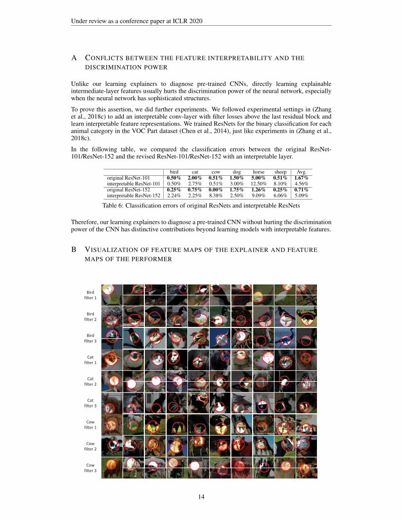
B VISUALIZATION OF FEATURE MAPS OF THE EXPLAINER AND FEATUREMAPS OF THE PERFORMER

14


Visualization of feature maps in the conv-interp-2 layer of the explainer. Each row correspondsto feature maps of a filter in the conv-interp-2 layer. We simply used a round RF for each neuralactivation and overlapped all RFs for visualization.

Visualization of feature maps in the conv-interp-2 layer of the explainer. Each row correspondsto feature maps of a filter in the conv-interp-2 layer. We simply used a round RF for each neuralactivation and overlapped all RFs for visualization.

15


Visualization of feature maps in the top conv-layer of the performer. Each row corresponds to featuremaps of a filter in the top conv-layer. We simply used a round RF for each neural activation andoverlapped all RFs for visualization.

C ENSURING THE EXPLAINER TO MIMIC THE PERFORMER

A high reconstruction quality ensures the explainer successfully mimics the signal processing inthe performer. Let us assume the explainer mistakenly uses an object part for prediction, whichthe performer does not use. Then, when we add or remove the target part from an testing image,the explainer will generate a obviously different feature, but the performer will not; vice versa. Inthis way, given sufficient training samples, a high reconstruction quality can ensures the explainerapproximate the logic of signal processing in the performer.

16


D GRAD-CAM ATTENTION MAPS

interpretable Ordinary interpretable Ordinary interpretable Ordinary interpretable Ordinary

Grad-CAM attention maps. We used (Selvaraju et al., 2017) to compute grad-CAM attention mapsof interpretable features of the conv-interp-2 layer in the explainer and those of ordinary featuresof the top conv-layer in the performer. Interpretable filters in the conv-interp-2 layer focused ondistinct object parts, while ordinary filters in the performer separated its attention to both texturesand parts.

The quantitative analysis in Figure 4 of the paper shows an example of how to use the disentangledobject-part features to quantitatively evaluate contributions of different parts to the output score ofobject classification. Based on prior semantic meanings of the interpretable filters, we show a priorexplanation of the logic in the classification without manually checking activation distributions ofeach channel of the feature map. Thus, this is different from the visualization of CNN representa-tions, which requires people to manually check the explanation based on visualization results.

E DETAILED RESULTS OF p VALUES

Pascal-Part dataset (Chen et al., 2014) CUB200-2011 (Wah et al., 2011)Single-category Multi-category

bird cat cow dog horse sheep Avg. Avg. Avg.AlexNet 0.75 0.72 0.69 0.72 0.70 0.70 0.71 – 0.5810VGG-M 0.81 0.80 0.81 0.80 0.81 0.81 0.81 0.9012 0.8611VGG-S 0.91 0.90 0.90 0.90 0.90 0.90 0.90 0.9270 0.9533VGG-16 0.88 0.89 0.87 0.87 0.86 0.88 0.87 0.8593 0.9579ResNet-101 0.98 0.97 0.97 0.97 0.98 0.97 0.97 – –ResNet-152 0.98 0.98 0.98 0.98 0.98 0.99 0.98 – –

Table 7: p values of explainers.

F MORE RESULTS OF LOCATION INSTABILITY

In this supplementary material, we add another baseline for comparison. Because we took fea-ture maps of the relu4 layer of the AlexNet/VGG-M/VGG-S (the 12th/12th/11th layer of theAlexNet/VGG-M/VGG-S) and the relu5-2 layer of the VGG-16 (the 28th layer) as target featuremaps to be explained, we sent feature maps of these layers feature into explainer networks to dis-entangle them. Thus, we measured the location instability of these target feature maps as the newbaseline.

The following two tables show that our explainer networks successfully disentangled these targetfeature maps, and the disentangled feature maps in the explainer exhibited much lower locationinstability.

17


Single-categorybird cat cow dog horse sheep Avg

AlexNet (the relu4 layer) 0.152 0.130 0.140 0.127 0.143 0.139 0.139AlexNet (the top conv-layer) 0.153 0.131 0.141 0.128 0.145 0.140 0.140Explainer 0.104 0.089 0.101 0.083 0.098 0.103 0.096VGG-M (the relu4 layer) 0.148 0.127 0.138 0.126 0.140 0.137 0.136VGG-M (the top conv-layer) 0.152 0.132 0.143 0.130 0.145 0.141 0.141Explainer 0.106 0.088 0.101 0.088 0.097 0.101 0.097VGG-S (the relu4 layer) 0.148 0.127 0.136 0.125 0.139 0.137 0.135VGG-S (the top conv-layer) 0.152 0.131 0.141 0.128 0.144 0.141 0.139Explainer 0.110 0.085 0.098 0.085 0.091 0.096 0.094VGG-16 (the relu5-2 layer) 0.151 0.128 0.145 0.124 0.146 0.146 0.140VGG-16 (the top conv-layer) 0.145 0.133 0.146 0.127 0.143 0.143 0.139Explainer 0.095 0.089 0.097 0.085 0.087 0.089 0.090

Table 8: Location instability of feature maps in performers and explainers. Performers are learnedbased on the Pascal-Part dataset (Chen et al., 2014)

AlexNet (relu4 layer) 0.1542AlexNet (the top conv-layer) 0.1502Explainer 0.0906VGG-M (relu4 layer) 0.1484VGG-M (the top conv-layer) 0.1476Explainer 0.0815VGG-S (relu4 layer) 0.1518VGG-S (the top conv-layer) 0.1481Explainer 0.0704VGG-16 (relu5-2 layer) 0.1444VGG-16 (the top conv-layer) 0.1373Explainer 0.0490

Table 9: Location instability of feature maps in performers and explainers. Performers are learnedbased on the CUB200-2011 dataset (Wah et al., 2011)

G ABOUT EVALUATION METRIC

The location instability is designed to evaluate the fitness between an intermediate-layer filter f andthe representation of a specific object part, and it has been widely used in (Zhang et al., 2018c;a).Therefore, we used this metric for evaluation in our experiments. In fact, there is another metric toidentify semantics of CNN filters, which was proposed by (Bau et al., 2017). This study annotatedpixel-level labels for six kinds of semantics (objects, parts, scenes, textures, materials, and colors)on testing images. Then, given a feature map of a filter f , they used the intersection-of-union (IoU)between activation regions in the feature map and image regions of each kind of semantics to iden-tify the semantic meaning of this filter. I.e. for filters oriented to representations of object parts, thismetric measures whether or not activation regions in a feature map greatly overlap to ground-truthsegment of a specific object part. However, in this study, we disentangled original feature mapsinto object parts without any ground-truth annotations of object parts. The disentangled object partsusually represent joint regions of ground-truth parts, sub-regions of ground-truth parts, or combina-tions of small ground-truth parts, although each disentangled object part consistently describes thesame part through different objects. Therefore, when filters are learned without ground-truth partannotations, the metric in (Bau et al., 2017) is less suitable to evaluate the object-part semantics thanthe metric of location instability (Zhang et al., 2018a).

H UNDERSTANDING OF FILTER LOSSES

According to (Zhang et al., 2019), we can re-write the filter loss as

Lossf = −H(P) +H(P′|X) +∑

xf∈Xp(P+, xf )H(P+|X = xf )

18


where P′ = {∅,P+}. H(P) = −∑µ∈P p(µ) log p(µ) is a constant prior entropy of part-location

candidates (here µ = ∅ is a dummy location candidate).

To compute above mutual information, p(µ) is defined as constant. p(xf |µ) is given as

p(xf |µ) = p(xf |Tµ) =1

Zµexp

[tr(xf · Tµ)

](3)

where Tµ denotes the part template corresponding to the part location µ, as shown in the followingfigure. Zµ =

∑xf

exp[tr(xf · Tµ)]. tr(·) indicates the trace of a matrix.

Conv‐interp

ReLU

Best fit this template

LossfLossfLossf

Feature maps

Part template Tµ corresponding to each part location µ (Zhang et al., 2019)

Low inter-category entropy: The second term H(P′ = {∅,P+}|X) is computed as H(T′ ={∅,P+}|X) = −

∑xfp(xf )

∑µ∈{∅,P+} p(µ|xf ) log p(µ|xf ), where P+ = {µ1, µ2, . . . , µL2} ⊂

P and p(P+|xf ) =∑L2

i=1 p(µi|xf ). We define the set of all valid part locations in P+ as a singlelabel to represent the category c. We use a negative template ∅ to denote other categories. This termencourages a low conditional entropy of inter-category activations, i.e. a well-learned filter f needsto be exclusively activated by a certain category c and keep silent on other categories. The featuremap xf can usually identify whether the input image belongs to category c or not, i.e. xf fitting toeither a valid part location µ ∈ P+ or ∅, without great uncertainty.

Low spatial entropy: The third term is given as H(P+|X = xf ) =∑L2

i=1 p(µi|xf ) log p(µi|xf ),where p(µi|xf ) =

p(µi|xf )p(P+|xf ) . This term encourages a low conditional entropy of spatial distribution

of xf ’s activations. I.e. given an image I ∈ Ic, a well-learned filter should only be activated bya single region µ ∈ P+ of the feature map xf , instead of being repetitively triggered at differentlocations.

Optimization of filter losses: The computation of gradients of the filter loss w.r.t. each element x(ij)f

of feature map xf is time-consuming. (Zhang et al., 2019) computes an approximate but efficientgradients to speed up the computation, as follows.

∂Lossf

∂x(ij)f

=∑µ∈P

p(µ)tijetr(xf ·Tµ)

Zµ

{tr(xf · Tµ)− log

[Zµp(xf )

]}≈p(µ)tij

Zµetr(xf ·T )

{tr(xf · T )− log[Zµp(xf )]

}where T is the target template for feature map xf . Let us assume that there are multiple object

categories C. We simply assign each filter f with the category c ∈ C whose images activate fthe most, i.e. c = argmaxcExf :I∈Ic

∑ij x

(ij)f . If the input image I belongs to the filter f ’s target

category, then T = Tµ, where µ= argmaxµ=[i,j]x(ij)f . If image I belongs to other categories, then

T = ∅. Considering ∀µ∈P \ {µ}, etr(xf ·T )� etr(xf ·Tµ) after initial learning epoches, we can makeapproximations in the above equation.

Note that above assignments of object categories are also used to compute location instability forintermediate-layer filters to evaluate their interpretability.

19


Inspired by optimization tricks in (Zhang et al., 2019), we updated the parameter λf =1

300NExf [‖

∂Lossrec∂xf

‖]/Exf [‖∂Lossf∂xf

‖] for the N -th learning epoch in an online manner, where∂Lossrec∂xf

denotes gradients of reconstruction losses obtained from upper layers. In particular, giv-en performers for single-category classification, we simply used feature maps of positive images(i.e. objects of the target category) to approximately estimate the parameter α for the norm-layer,because positive images can much more strongly trigger interpretable filters than negative images.Thus, computing α based on positive images made p accurately measure the contribution ratio of theinterpretable track when the network made predictions to positive images. We will clarify all thesesettings when the paper is accepted. In experiments, for interpretable filters in the conv-interp-2layer, we added the filter loss to x′f = p · xf + (1− p) · xordin, where xordin ∈ RL×L denotes a channelof xordin that corresponds to the channel of filter f . We found that this modification achieved morerobust performance than directly applying the filter loss to xf . In this case, the filter loss encourageda large value of p and trained the interpretable filter f , but we did not pass gradients of the filter lossto the ordinary track.

I ABOUT PARAMETER SETTINGS

In the experimental section, we have clarified settings for parameters. We simply set η = 1.0× 106

for the AlexNet, VGG-M, and VGG-S without sophisticatedly turning the value of η. We set η =1.5×105 for the VGG-16, since the VGG-16 has more conv-layers than the other networks. For eachtype of CNNs, the same value of η was uniformly applied to various CNNs for different categories.Our method is not sensitive to η. When the VGG-16 used the η value of the AlexNet, it only changedan average location instability of 0.003 over all experiments.

J EVALUATING THE RECONSTRUCTION QUALITY BASED ON THEOBJECT-CLASSIFICATION ACCURACY

In order to evaluate the feature-reconstruction quality, we used the classification accuracy basedon explainer features as an evaluation metric. We fed output features of the explainer back to theperformer for classification. Theoretically, a high classification accuracy may demonstrate that theexplainer can well reconstruct performer features without losing much information. Note that ex-plainers were learned to reconstruct feature maps of performers, rather than optimizing the classifi-cation loss, so explainers could only approximate the classification performance of performers butcould not outperform performers.

In addition, we added another baseline, namely Explainer+cls, which used the object-classificationloss to replace the reconstruction loss to learned explainer networks. Thus, output features of Ex-plainer+cls exhibited higher classification accuracy than features of the original explainer.

The following table compares the classification accuracy between the performer and the explainer.For multi-category classification, the performance of explainers was quite close to that of perform-ers. Learning explainers with classification losses exhibited significantly better classification perfor-mance than learning explainers with reconstruction losses. Because Explainer+cls directly learnedfrom the classification loss, Explainer+cls sometimes even outperformed the performer.

Pascal-Part (Chen et al., 2014) CUB200 (Wah et al., 2011)Multi-category Single-category

Performer Explainer Explainer+cls Performer Explainer Explainer+cls Performer Explainer Explainer+cls

AlexNet – – – 4.60% 8.20% 2.88% 4.41% 10.98% 3.57%VGG-M 6.12% 6.62% 5.22% 3.18% 8.58% 3.40% 2.66% 6.84% 2.54%VGG-S 5.95% 6.97% 5.43% 2.26% 10.97% 3.86% 2.76% 8.53% 2.72%VGG-16 2.03% 2.17% 2.49% 1.34% 6.12% 1.76% 1.09% 6.04% 0.90%

Table 10: Classification errors based on feature maps of performers and explainers.

20

Q D U STANDING PART INFORMATION IN CNNS

Documents

Transcript of Q D U STANDING PART INFORMATION IN CNNS