Q# and NWChem: Tools for Scalable Quantum Chemistry on Quantum Computers

Guang Hao Low,1, ∗ Nicholas P. Bauman,2 Christopher E. Granade,1 Bo Peng,2 Nathan Wiebe,1 Eric J. Bylaska,2 DaveWecker,1 Sriram Krishnamoorthy,2 Martin Roetteler,1 Karol Kowalski,2 Matthias Troyer,1 and Nathan A. Baker2

1Microsoft Research, Quantum Architectures and Computation Group, Redmond, Washington 98052, USA2Pacific Northwest National Laboratory, Richland, Washington 99354, USA

(Dated: April 3, 2019)

Fault-tolerant quantum computation promises to solve outstanding problems in quantum chem-istry within the next decade. Realizing this promise requires scalable tools that allow users to trans-late descriptions of electronic structure problems to optimized quantum gate sequences executed onphysical hardware, without requiring specialized quantum computing knowledge. To this end, wepresent a quantum chemistry library, under the open-source MIT license, that implements and enablesstraightforward use of state-of-art quantum simulation algorithms. The library is implemented in Q#,a language designed to express quantum algorithms at scale, and interfaces with NWChem, a lead-ing electronic structure package. We define a standardized schema for this interface, Broombridge,that describes second-quantized Hamiltonians, along with metadata required for effective quantumsimulation, such as trial wavefunction ansatzes. This schema is generated for arbitrary moleculesby NWChem, conveniently accessible, for instance, through Docker containers and a recently devel-oped web interface EMSL Arrows. We illustrate use of the library with various examples, includingground- and excited-state calculations for LiH, H10, and C20 with an active-space simplification, andautomatically obtain resource estimates for classically intractable examples.

CONTENTS

I. Introduction 2

II. Review 4A. Quantum computing and programming 4B. Quantum chemistry 8C. Quantum simulation 13

III. The Broombridge schema for representing electronic structure problems 19A. Broombridge v0.1 specifications 19B. Generating Broombridge with NWChem 21

IV. Simulating quantum chemistry with the Microsoft Quantum Development Kit 21A. Constructing qubit Hamiltonians from chemistry Hamiltonians 21B. Synthesizing quantum simulation circuits 23C. Estimating eigenvalues 24

V. Example applications 25A. Lithium hydride ground- and excited-state energies 25B. Empirical Trotter error estimation of stretched H10 chains 27C. Quantum computing predictions and resource estimations for C20 isomerizations 29

VI. Conclusions 32

Acknowledgments 32

References 33

A. Running examples 36

∗ guanghao.low@microsoft.com

arX

iv:1

904.

0113

1v1

[qu

ant-

ph]

1 A

pr 2

019

2

I. INTRODUCTION

Computational chemistry is one of the main consumers of computing resources today. Computational chem-istry calculations generally aim to approximate electronic structure Schrödinger equation solutions to “chemicalaccuracy” (defined in Sec. II A): where predicted computed chemical properties quantitatively match experimen-tal observations. There have been great successes in the field, heralded by celebrated techniques such as densityfunctional theory (DFT) [1], coupled-cluster (CC) theory [2], or density matrix renormalization group (DMRG) [3].However, chemical accuracy remains beyond the reach of tractable classical computing techniques for numerousproblems, often involving transition metals and excited states. In particular, a brute-force computational approach tothe Schrödinger equation has exponential cost arising from the curse of dimensionality, and is generally infeasible—for both current and projected supercomputers—for chemical systems beyond a hundred spin orbitals.

Quantum computing [4] promises a solution to this fundamental challenge of accurate electronic structure calcula-tions. Instead of simulating the time-evolution of electrons according to the laws of quantum mechanics on classicalTuring-machine computers, quantum computers natively realize quantum effects at a hardware level. The inher-ent computational power of quantum systems provides hope of solving the hardest quantum mechanical problemsin chemistry and material science, such as the mechanism of biological nitrogen fixation [5] or high-temperaturesuperconductivity [6, 7].

The theoretical details of quantum algorithms for electronic structure calculations have been studied extensively.The first explicit algorithm for simulating generic local Hamiltonians was by Lloyd [8], which has since seen con-tinual improvements and generalizations [9–17]. These algorithms have been specialized to fermionic systems [18],especially that of chemistry [19, 20], along with numerous case studies [21–26], and novel quantum-classical hy-brid schemes that trade-off quantum circuit depth for at least polynomially more rounds of classical repetition andpost-processing [7, 27, 28]. A more thorough overview can be found in other publications [29].

However, the practical details of using quantum methods for many real-world chemistry and material science prob-lems pose unique challenges. Setting aside the availability of fault-tolerant quantum hardware, and the difficultyof controlling said devices, it is non-trivial to program quantum devices to achieve a desired effect. Paralleling thehistory of classical computing, quantum computing requires significant software development effort before domainexperts can apply quantum resources to their problems at scale. This need has motivated the recent development ofa variety of quantum programming languages [30–34], each of which makes feasible and accessible various aspectsof quantum software development. Building on this, a number of different libraries for quantum chemistry appli-cations have been developed [35, 36], in or for use with quantum programming frameworks, focusing primarily onnear-term quantum chemistry tasks for Noisy Intermediate-Scale Quantum (NISQ) [37] devices.

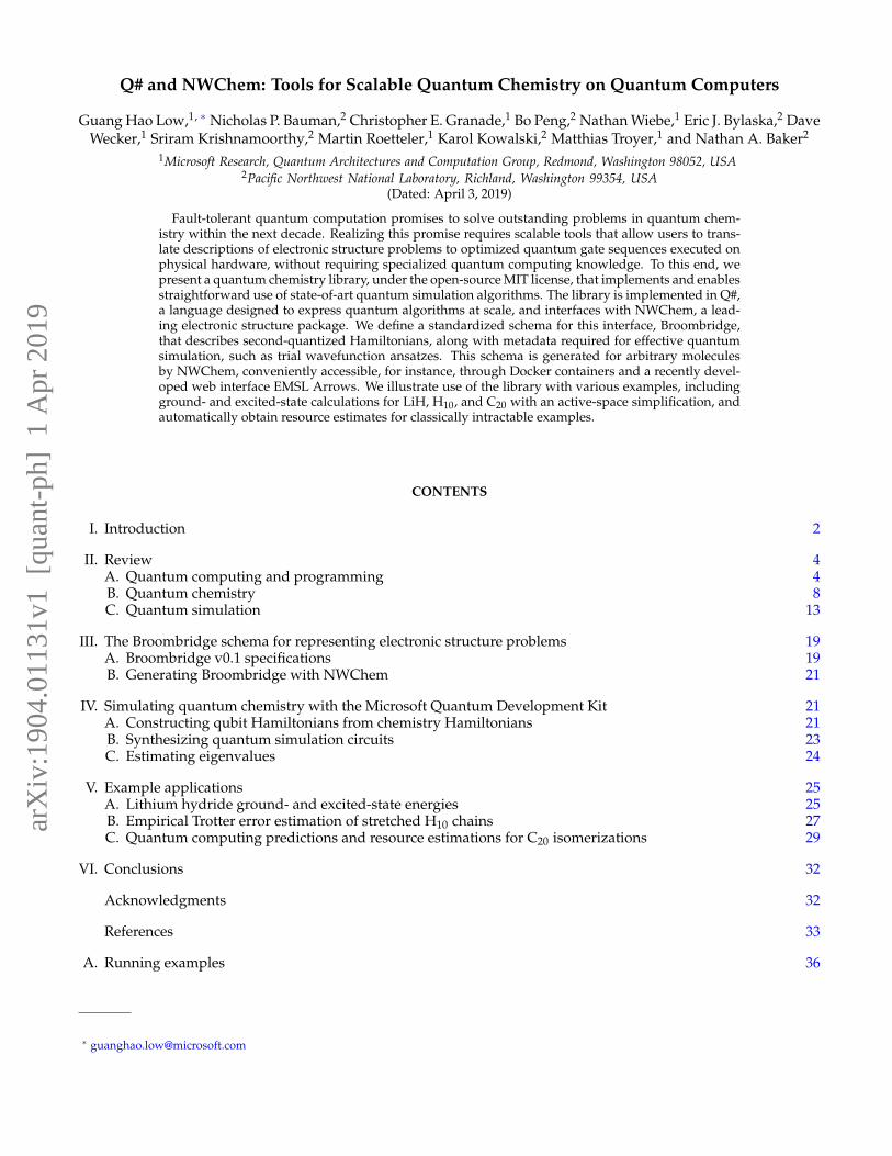
In this paper, we present a software suite outlined in Figure 1 that empowers quantum chemistry experts to writequantum simulation code that can be tested and costed using a classical computer as well as be executed as written ona fault-tolerant quantum computer once one becomes available. We accordingly focus on these future applications,as well as developing technologies that allow us to today simulate and profile resources needed for fault-tolerantquantum simulations. The quantum simulation software we provide interacts with the underlying quantum error-correcting code and, in turn, the physical qubits through an abstraction that we call a simulator. The simulator canbe easily swapped with genuine hardware, guaranteeing that our code can be reused once fault-tolerant quantumhardware becomes available. We have designed our quantum simulator software so that solutions are amenable touse by domain experts in quantum chemistry, without requiring strong domain expertise in quantum computingand quantum algorithms. This focus is especially critical as we transition from preliminary investigations—such asthe use of quantum devices to study ground-state energies of relatively simple molecules [38]—to applications suchas studying higher-energy properties and more complicated systems.

NWChem:Electronic structure

modelling

Quantum Development Kit chemistry library:

Simulation algorithms for fermions

Broombrige:YAML-based Serialization

Quantum application:Classical host & other Q# operations

Quantum Development Kit canon library:

Quantum algorithm building blocks

Target machines:Quantum computer / simulator /

resources estimator / ...

Figure 1. Workflow for simulating quantum chemistry on quantum computers using NWChem and Microsoft Quantum De-velopment Kit libraries. Our main contributions, Broombridge and the chemistry library, are shaded. See Figure 2 for a detailedbreakdown.

3

Making effective use of quantum computing resources past this transition puts a more significant demand on soft-ware development and interoperability between different pieces in a complete workflow. We address this demandby introducing Broombridge, a new serialization format for representing fermionic Hamiltonians. Broombridge en-ables interoperation between North-West Chemistry (NWChem) modelling software [39], a leadership-class suite oftools for modeling quantum chemistry problems, and the Microsoft Quantum Development Kit [34], a software plat-form for implementing quantum algorithms for both simulated execution and execution on eventual fault-toleranthardware. Our reproducible workflow shown in Figure 1 automates simulations of large families of molecules. Thisworkflow begins with NWChem, and its recent optional web interface Environmental Molecular Science Laboratory(EMSL) Arrows, which serializes descriptions of electronic structure problems as Broombridge. Broombridge is thenconsumed by our quantum chemistry library in the Microsoft Quantum Development Kit, which is used in appli-cations invoking quantum simulation and other supporting quantum algorithms. As seen in the flowchart, manyintermediate choices that affect performance and accuracy can be made between the initial problem specificationand the final simulation on hardware. Ultimately, the software should free users from these fine details, and allowthem to focus on the scientific endeavor.

We illustrate this interoperability through a series of examples, including the basic examples traditionally used tointroduce quantum chemistry development as well as examples motivated by future quantum simulation applica-tions. In particular, we highlight features in the Broombridge schema that enable us to conveniently describe thequantum Hamiltonian as well as the initial guesses for the eigenstate in question, which includes excited states thatare traditionally difficult to probe by variational approaches. These features are illustrated in example simulationsof excited states of LiH and standard problems such as obtaining correlation energies of the hydrogen chain H10,and energy calculations of different C20 isomer configurations calculated using small active spaces. We highlight theability of the quantum chemistry library to perform gate count estimates for a challenging example, specifically a full-configuration interaction simulation of C20 in a 100 spin-orbital active space. Such simulations are beyond the reachof any classical computer, but are expected to be tractable for quantum computers. These examples demonstrate thevalue of our system: in addition to simplifying quantum resources counts and electronic structure simulations, it alsoenables large-scale surveys of quantum chemistry simulations that have hitherto been too challenging to perform byhand.

The layout of the paper is as follows. We begin in Section II with a review of quantum computing as well asquantum chemistry. In particular, we review state-of-the-art quantum simulation methods, such as qubitization andTrotter formulas, as well as methods for phase estimation. Important software such as Q# and NWChem are also re-viewed. In Section III, we introduce the Broombridge schema used to interface NWChem with Q#, and demonstrate

Real-world problemsReal-world problems

NanostructuresBiomolecules MaterialsNanostructuresBiomolecules Materials

Real-world problems

NanostructuresBiomolecules Materials

Domain specific knowledgeReaction rates and pathways

Ground and excited states

Domain specific knowledgeReaction rates and pathways

Ground and excited states

Broombridge database

Jordan-Wigner mapping

Jordan-Wigner mapping

Algorithm-specific optimizations

Algorithm-specific optimizations

Quantum state preparation

QROMRejection sampling

Simulation algorithms

Qubitization

T-gate-count optimized

Qubit-count optimized

SBM ...

Trotter—Suzuki

Arbitrary even order

First order

Phase estimation

RobustQuantum ...

Simulation algorithms specialized to electronic structureSimulation algorithms specialized to electronic structure

NWChem:Electronic structure

modelling

Quantum Development Kit

chemistry library:

Simulation algorithms for

fermions

Electronic structure representation and

metadataFormat validator

Broombrige:YAML-based Serialization

Trial wavefunction Ansatz

Electronic structure Hamiltonian

Relevant metadata

Fermion representation

Trial wavefunction Ansatz

Electronic structure Hamiltonian

Relevant metadata

Fermion representation

Trial wavefunction Ansatz

Electronic structure Hamiltonian

Relevant metadata

Qubitrepresentation

Trial wavefunction Ansatz

Electronic structure Hamiltonian

Relevant metadata

Qubitrepresentation

Basis set

Plane wavesGaussians

Basis set

Plane wavesGaussians

Quantum Development Kit

canon library:Quantum algorithm

building blocks

Q# operations and functions

C# host program

Quantum application

Quantum computer

Full-statesimulator

Target machines

Figure 2. Detailed workflow for simulating quantum chemistry on quantum computers.

4

how Broombridge may be produced. Section IV provides a high-level discussion that shows how to use these toolstogether to simulate molecules within the Microsoft Quantum Development Kit chemistry simulation library. Weprovide concrete examples of the library in action in Section V and use our tools to study the electronic states of LiH,H10, and C20 using quantum algorithms simulated on classical computers, as well as provide resource estimates forsimulations of hard molecules before concluding. Finally, we conclude in Section VI with our perspective of futuredirections for this line of work.

II. REVIEW

The exponential growth of classical computing capabilities projected by Moore’s law is coming to an end [40].However, many computational problems of scientific and technological interest remain out of reach. In light of this,quantum computing has emerged—amongst various technologies—as the leading contender for continued progressdue to its potential for realizing further exponential speedups, at least for certain specialized problems. The centralidea is to develop a device that can, within arbitrarily small error, implement at least a universal set of quantumtransformation on a quantum state. This suffices to capture the computation power of practical quantum computing,encapsulated by the complexity class BQP.

Of all the applications of quantum computing, the quantum simulation of physics, chemistry, and materials isenvisioned to be the most transformative; one of the earliest useful areas for quantum advantage. Since the dynamicsof quantum systems are given by unitary transformations, we can in principle compile these dynamics, representedby Hamiltonians, into a sequence of discrete gates on a quantum computer. This approach can yield exponentialspeedups over the best known classical algorithms for simulating hard quantum problems, such as those in catalysisor material science.

We review the key concepts of quantum computation based on qubits in Section II A, together with an overviewfor implementing and execution quantum algorithms in the Q# programming language. Subsequently, we statethe fundamental concepts and definitions underlying quantum chemistry problems in Section II B, with a focus onits fermionic second-quantized representation, and the use of NWChem. The ideas of quantum computation andquantum chemistry are merged in Section II C, which outlines the map from fermions to qubit, and the algorithmsthat simulate quantum Hamiltonian on a quantum computer.

A. Quantum computing and programming

Before describing the compilation of quantum simulation algorithm for Hamiltonian dynamics into primitiveoperations on quantum computing, we need to discuss the elementary units of quantum memory, and the targetgate set of compilation. The fundamental unit of memory in a quantum computer is a qubit. A qubit is much likea probabilistic classical bit. It can take the values 0 or 1, which we denote by the orthonormal two-dimensionalcolumn vectors |0〉 and |1〉. The quantum state for a qubit can be an arbitrary quantum mixture of these two states;the simplest example is known as a “pure” quantum state. For a qubit, the pure quantum state takes the form of acomplex unit vector a|0〉+ b|1〉 = [a b]T . An ordinary probabilistic classical bit would have positive probabilities aand b that sum to 1; however, a pure quantum state has a, b ∈ C and |a|2 + |b|2 = 1.

Just as measurement causes the prior distribution over the value of a classical stochastic bit to collapse to either0 or 1, measurement of a quantum bit causes a similar impact on the quantum state. The principal difference fromthe classical case is that Pr [0] = |a|2 for the quantum example, rather than Pr [0] = a as in the classical case. Theexponentially greater power of quantum computers stems largely from this subtle difference. As a, b ∈ C and—moreimportantly—can be negative, the different possible configurations that a register of qubits can be in can interferewith each other. From this perspective, quantum computing can be viewed as the art of introducing and exploitingquantum interference for computational purposes.

The quantum state for multiple qubits can be represented by a tensor product of single qubit states. This meansthat, while a single qubit state is described by a two-dimensional vector space C2, a two-qubit state lives on a four-dimensional vector space C22

. In general, an n-qubit quantum state exists on a vector space C2nof dimension 2n. This

is unsurprising as a classical probability distribution over n bits is also spanned by exponentially many bit strings.Interference between the possible configurations of a quantum system is engineered using quantum gates. Perhaps

the most important defining characteristic of a quantum computer is the existence of a “universal quantum gate set”.This set consists of operations that can approximate, within arbitrarily small error, any transformation permitted byquantum mechanics on qubit states. These legal transformations are represented as unitary matrices, which preservethe lengths of vectors, conserve the value of |a|2 + |b|2 for qubits, and hence conserve probability. In principle,

5

arbitrary single-qubit rotations and an entangling gate such as a controlled-NOT can be used to generate any unitarytransformation. If we take |0〉 = [1 0]T and |1〉 = [0 1]T , then these single qubit rotations can be easily expressed asexponentials of the following single-qubit Pauli operations

1 =

[1 00 1

], X =

[0 11 0

], Y =

[0 −ii 0

], and Z =

[1 00 −1

]. (1)

These Paulis can be interconverted using products of Clifford gates called the Hadamard and phase gate:

HAD =1√2

[1 11 −1

], S =

[1 00 i

]. (2)

The notion of a single-qubit rotation is similarly a convenient concept in quantum computing. The analogue of arotation about the z-axis for a quantum bit for an angle θ can be expressed as

RZ(θ) = e−iZθ/2 = cos (θ/2)1− i sin (θ/2)Z =

[cos (θ/2) −i sin (θ/2)−i sin (θ/2) cos (θ/2)

]. (3)

Any-single qubit operation can be expressed as a sequence of three rotations: RZ(θ) · RX(φ) · RZ(ψ) = RZ(θ) ·HAD · RZ(φ) ·HAD · RZ(ψ) for appropriate Euler angles θ, φ and ψ. In fault-tolerant applications, these rotations aretypically approximated by sequences of HAD and T =

√S gates.

The simplest two-qubit quantum gate is the controlled-NOT gate controlled by qubit j and applied to qubit k,which has the action |0〉j |x〉k 7→ |0〉j |x〉k and |1〉j |x〉k 7→ |1〉j |x⊕ 1〉k. The gate takes the following matrix represen-tation (using the above basis convention)

CNOTjk =

1 0 0 00 1 0 00 0 0 10 0 1 0

. (4)

It can be useful to observe that gates in the Clifford group {HAD, S, CNOT} can map any n-qubit Pauli P ∈{1, X, Y, Z}⊗n operator to any other n-qubit Pauli by conjugation. This provides one possible, though not nec-essarily the most efficient, implementation of RP(θ) = e−iPθ/2 which is commonly found in quantum simulationalgorithms.

Thinking about quantum simulation algorithms strictly in terms of these operations is quite taxing, just as pro-gramming a word processor using only assembly code would be a challenge in classical computing. Higher-levelquantum programming languages have been developed to address these challenges [30–32, 34]. These languagesbridge the gap between the low-level physics-inspired description of the quantum states and the higher level de-scriptions of algorithms that are customarily shown as pseudocode in quantum computing papers. Such bridges areessential not only because the act of compiling a quantum algorithm into an optimized sequence of quantum gates isdemanding, but also because a quantum computer is not just a single monolithic device. A quantum computer is arich nested stack of computing substrates that view the quantum computer at different levels of abstraction: a fault-tolerant quantum computer provides a user with a view of logical qubits that are made out of collections of physicalqubits which are themselves an abstraction of the basic physical systems that lie beneath all held within an errorcorrecting code wherein the quantum gates actually represent complex sequences of physical gates. Given this com-plexity, one quickly realizes that high-level quantum programming languages are not a luxury, but a necessity—evenbefore quantum computing comes of age.

1. Developing quantum algorithms in Q#

Our aim is to show how simulations of quantum chemistry can be made easier by using the Microsoft QuantumDevelopment Kit in conjunction with NWChem. Here we will review the Microsoft Quantum Development Kitwhich provides a new language, Q#, that is used to program the quantum chemistry simulations in this paper.The Microsoft Quantum Development Kit is distributed under the open-source MIT license as a set of installablepackages for .NET Core, an open-source cross-platform programming environment that includes high-level classicallanguages such as C# and F#.

Quantum programs written in Q# use an accelerator model, similar to graphics programming or the use of field-programmable gate arrays. As illustrated in Figure 3, once a user writes Q# code, that program can be dispatched

6

Figure 3. Execution model used by the Microsoft Quantum Development Kit to interact with target machines, each of whichexecutes Q# code on behalf of a classical program written in a .NET Core language such as C#.

to one of several target machines by a host program written in any .NET Core language. The target machine thenruns the Q# program, including both classical logic and quantum instructions, and returns its result to the classicalhost program. Each target machine exposes a set of available instructions to Q# programs as operations that can becalled during a program’s execution. For instance, the Hadamard gate can be applied by calling the H operation inthe Microsoft.Quantum.Primitive namespace. The operations that define the interface between a Q# program and targetmachines are collectively known as the prelude, and can be referenced in a Q# source file using an open statement.

In Listing 1, we show a simple example of using the Microsoft Quantum Development Kit to program a quantumrandom number generator (QRNG). At Line 9, the user declares a new operation, Qrng, that can interact with thetarget machine in a variety of ways, including allocating fresh qubits, or calling primitive operations. Once definedin this way, Qrng can be called from other operations, or can be invoked from a classical host program written inC# or another .NET Core language. For a complete set of samples demonstrating this process, please see https://github.com/Microsoft/Quantum.

// All Q# code l i v e s i n s i d e of a namespace , so we begin by dec lar ing t h a t namespace here .namespace Qrng {

// We can import names from other namespaces using the open keyword .open Microsof t . Quantum . P r i m i t i v e ;

5

/// # Summary/// Prepares a qubit in the |+〉 s t a t e , then measures in the Z b a s i s to obta in a random b i t .// This l i n e d e c l a r e s an operat ion t h a t takes no inputs and re turns a Resul t .operation Qrng ( ) : Result {

10 mutable r e s u l t = Zero ;// The using keyword asks the t a r g e t machine f o r a f r e s h qubit , i n i t i a l l y in the |0〉 s t a t e .using ( qubit = Qubit ( ) ) {

// Applying the H operat ion to a qubit in the |0〉 s t a t e prepares t h a t qubit in the H |0〉 = |+〉↪→ s t a t e .

H( qubit ) ;15 // We can measure our qubit in the Z−b a s i s using the M operat ion provided by the prelude .

s e t r e s u l t = M( qubit ) ;// Before re turning the qubit to the t a r g e t machine , we need to make sure t h a t i t i s in the |0〉

↪→ s t a t e . This can be done using a c l a s s i c a l l y c o n t r o l l e d X gate , which we apply using a↪→ c l a s s i c a l if s tatement and the X operat ion .

i f ( r e s u l t == One) { X( qubit ) ; }}

20 // F i n a l l y , we return our random b i t to the c l a s s i c a l host program .return r e s u l t ;

}}

Listing 1. A simple quantum random number generator (QRNG) written in Q#. examples/qrng/qrng.qs

The Microsoft Quantum Development Kit also includes a set of standard libraries known as the canon that arebuilt up within Q# itself. These libraries provide Q# programs with useful routines for performing measurementsand manipulating flow control, as well as for higher-level quantum algorithms such as the quantum Fourier trans-form (QFT), implementations of phase estimation algorithms, and routines for quantum simulation algorithms. Acomplete reference to the prelude and canon is available online at https://docs.microsoft.com/qsharp/api/. Thefunctions and operations in the canon, together with other features of the Q# language—such as the Adjoint functor

7

to automatically transform an operation into its inverse operation, make it straightforward to encapsulate and reusecode in quantum applications.

2. Running Q# quantum algorithms

Once a quantum program has been written using Q#, it can be run using a classical host program to allocate atarget machine. This host will often be written in C#, but any other .NET Core language can be used. To demonstrate,we use an excerpt in Listing 2 from the example of quantum teleportation, which is described in detail within thecomplete source file.

/// # Summary/// Runs the Telepor t operat ion above by a l l o c a t i n g three qubits ,/// and a s s e r t i n g t h a t the message qubit i s c o r r e c t l y t e l e p o r t e d .operation RunTeleport ( ) : Unit {

5 using ( ( msg , here , there ) = ( Qubit ( ) , Qubit ( ) , Qubit ( ) ) ) {// We’ l l prepare a s t a t e |+〉 = H |0〉 by using// the H operat ion .H(msg) ;// After t e l e p o r t i n g using the Teleport operation ,

10 // the t a r g e t qubit should be in the |+〉 s t a t e . Thus ,// applying another H w i l l transform i t back i n t o the// |0〉 s t a t e .Te lepor t (msg , here , there ) ;H( there ) ;

15 // When run on a simulator , we can a s s e r t t h i s f a c t// using the AssertQubit operat ion . In other cases , t h i s// operat ion i s s a f e l y ignored s i n c e i t has no e f f e c t .AssertQubit ( Zero , there ) ;

}20 }

Listing 2. An example of quantum teleportation between two qubits written in Q#. examples/teleport/Teleport.qs

In many cases, we want to run our quantum programs on a simulator that will let us check that they operate correctlyon noiseless qubits. The Microsoft Quantum Development Kit provides the QuantumSimulator target machine for thiscase, as demonstrated in Listing 3. Full details on running this example can be found in Section A of the appendix.

The QuantumSimulator target machine is especially useful in conjunction with unit testing frameworks such as xU-nit [41], as this makes it possible to write a comprehensive set of tests for a quantum algorithm implementation.Such test suites help build confidence that an implementation is correct.

Once we are confident that a Q# program functions correctly, the next steps often involve costing out larger casesthat are intractable with only classical resources. The Microsoft Quantum Development Kit offers another targetmachine, the QCTraceSimulator class, which counts the resources required to run a quantum program. We demonstratethe use of this target machine in Listing 3 as well.

// C# programs used as c l a s s i c a l hosts f o r Q# programs// can be wri t ten as t y p i c a l console a p p p l i c a t i o n s .s t a t i c void Main ( s t r i n g [ ] args ){

19 // We can a l l o c a t e the QuantumSimulator t a r g e t// machine by i n s t a n t i a t i n g a new i n s t a n c e . The using// block makes sure t h a t the new t a r g e t machine// i s c o r r e c t l y d e a l l o c a t e d at the end .using ( var qsim = new QuantumSimulator ( ) )

24 {// The Q# compiler exposes operat ions and f u n c t i o n s// as .NET c l a s s e s , each of which has a s t a t i c method// Run t h a t accepts a t a r g e t machine and runs the// funct ion or operat ion on t h a t machine .

29 // Since t a r g e t machines re turn t h e i r r e s u l t s asynchronously ,// we use the Wait method to make sure t h a t the// operat ion has completed .RunTeleport . Run( qsim ) . Wait ( ) ;

}34

// In the same way , we can i n s t a n t i a t e a new QCTraceSimulator

8

// t a r g e t machine to t r a c e the resources required by the RunTeleport// operat ion .var traceSim = new QCTraceSimulator (

39 // The t r a c e s imulator takes a c o n f i g u r a t i o n o b j e c t t h a t d e s c r i b e s// what c o s t s we would l i k e to t race , and how the t r a c e s imulator// should handle measurements . For more d e t a i l s , see// https://docs.microsoft.com/quantum/machines/qc-trace-simulator/ .new QCTraceSimulatorConfiguration

44 {usePrimit iveOperat ionsCounter = true ,throwOnUnconstraintMeasurement = f a l s e

}) ;

49

// Once we have our t r a c e simulator , we can run our operat ion in the// same way . After running , we can ask about the c o s t s required .RunTeleport . Run( traceSim ) . Wait ( ) ;var nCNOTs = traceSim . GetMetric <RunTeleport >( PrimitiveOperationsGroupsNames .CNOT) ;

54 System . Console . WriteLine ( $ " Used {nCNOTs} CNOT operat ions . " ) ;

}

Listing 3. Classical host for Listing 2. examples/teleport/Host.cs

Critically, the Q# code run in both parts of Listing 3 is identical: the RunTeleport operation cannot observe whetherit is is being simulated by QuantumSimulator or QCTraceSimulator. That is, the choice of target machine is transparent toQ# code as it is being run, allowing us to build confidence by testing with small classical resources, and then reusethe same code in cost estimation and—eventually—in actual hardware.

B. Quantum chemistry

The main focus of quantum chemistry is providing computational tools for modeling molecular structure, chem-ical reactions, dynamics, and spectroscopic properties. These are inextricably linked to many-body methods forsolving the stationary (time-independent) Schrödinger equation

H |Ψ〉 = E |Ψ〉 , (5)

where H, |Ψ〉, and E represent the Hamiltonian operator, wavefunction, and corresponding energy of a molecularsystem (respectively). The energy scale of interest in these problems is typically on the order of 1 Hartree, which weshall use as our units for energy and inverse-time in the following. In general, eigenvectors and eigenvalues of theSchrödinger equations (|Ψ〉 and E, respectively) describe ground or excited electronic states. By applying variousassumptions regarding the nature of the inter-electron interactions and the algebraic form of the electronic wave-function, a plethora of various approximate methods have been introduced and tested over the last century. Thesemethods find approximate solutions to Schrödinger equations, and their underlying assumptions intrinsically de-fine the memory requirements and numerical overheads of simulating approximate many-body models on classicalmachines.

Among the several classes of many-body methodologies, a number of approaches stand out. These include thenumerous variants of Hartree–Fock (HF) and DFT methods, many-body perturbation theory (MBPT), Green’s func-tion methods (GF), configuration interaction (CI) and CC methods, density matrix theory, and DMRG approaches.Over the years, these methods have evolved into staple working engines used in numerous simulations of chemicalprocesses. A significant effort has also been directed towards the development of reduced scaling methods and em-bedding formulations to handle correlation effects in large molecular systems. The widespread use of these methodshas emphasized the role played by the proper inclusion of complex electron correlation effects for a comprehen-sive and accurate understanding of molecular processes. In some cases, for example CI and CC theories, achieving“chemical accuracy” of roughly

Chemical accuracy = 10−3 Hartree = 0.02721 eV = 2.625 kJ/mol = 316.8 kBKelvin, (6)

requires including enormous numbers of wavefunction parameters, which results in a steep computational com-plexity scaling of these formalisms. In asymptotic limit of the Full CI (FCI) formulation, the number of wavefunctionparameters scales as N! with respect to system size N. Examples that appear to require reaching this limit in-clude modeling low-spin open-shell systems, radicals, transition metal oxides, and actinides. Fortunately, quantumcomputing, which has polynomial scaling in N, offers means to address the exponential scaling of high-accuracywavefunction formulations on classical computing platforms.

9

1. Second-quantized Hamiltonians

The language of second quantization has permeated almost the entire area of quantum chemistry and it is widelyused to classify various many-body effects contributing to complex inter-electron correlation effects. Second quan-tization has also become a foundation for diagrammatic representation of various many-body theories. The cen-tral role in quantum chemistry is played by the Born–Oppenheimer approximation, where the electronic structureHamiltonian H describes electrons that move within a fixed nuclear frame

H =η

∑i=1

(−∇2

i2−∑

l

Zl|ri − Rl |

)+

η

∑i<j

1|ri − rj|

, (7)

where ∇2 is the Laplacian, Zl and Rl are the charge and position of the l-th nucleus, and ri is the position of the i-thelectron. In this basis, the corresponding η-electron wavefunction has components Ψ(x1, x2, . . . , xη) = 〈x1x2 . . . xη |Ψ〉indexed by the spatial and spin coordinates of i-th electron, i.e., xi = (ri, si) where ri ∈ R3 and si ∈ {↑, ↓}.

As |Ψ〉 describes of indistinguishable fermions (electrons), it also has to satisfy fermion statistics associated withits antisymmetry upon swapping the coordinates of any pair of electrons. Second-quantization techniques and theoccupation number representation provide a concise way of characterizing many-body effects in the Hamiltonianoperator and electronic wavefunction while automatically assuring its anti-symmetry. In the second-quantization,all operators and the many-body wavefunction are represented in terms of creation and annihilation operators a†

pand ap indexed by p. These operators satisfy the of anti-commutation relations

{ap, aq} = {a†p, a†

q} = 0, and {ap, a†q} = δpq. (8)

Additionally, when acting with any annihilation operator on the physical vacuum state |0〉 or when the creationoperator is applied to an occupied state, the following is always satisfied

∀p, ap |0〉 = a†p |1〉p = 0. (9)

Similarly, if the annihilation operator is applied to an occupied state or if the creation operator is applied to thevacuum then particles are destroyed or created respectively:

∀p, a†p |0〉 = |1〉p , ap |1〉p = |0〉p . (10)

Using these operators, one can represent the Hamiltonian operator as

H = ∑pq

hpqa†paq +

12 ∑

p,q,r,shpqrsa†

pa†q aras, (11)

The connection to the electronic structure Hamiltonian of (7) is completed by choosing p = (i, s) ∈ {1, · · · , M} ×{↑, ↓} to index one of M carefully chosen orbitals with amplitude φi(r) = 〈r|φi〉 in the position basis, and a spinstate with amplitude χs. In other words, a†

p creates an electron in one of N = 2M single-particle spin-orbitals|ψp〉 = |φi〉 |χs〉. The coefficients of (11) are then

hpq ≡ h(i,s1)(j,s2)= 〈ψp|

(−∇

2

2−∑

l

Zl|r− RI |

)|ψq〉 = δs1s2

∫dr φ∗i (r)

(−∇

2

2−∑

l

Zl|r− RI |

)φj(r)︸ ︷︷ ︸

hij

, (12)

hpqrs ≡ h(i,s1)(j,s2)(k,s3)(l,s4)= 〈ψp| 〈ψq|

1|r1 − r2|

|ψr〉 |ψs〉 = δs1s4 δs2s3

∫dr1dr2

φ∗i (r1)φ∗j (r2)φk(r2)φl(r1)

|r1 − r2|︸ ︷︷ ︸hijkl

. (13)

A convenient way of representing electronic wavefunction vector |Ψ〉 is then as as a linear combination of allsymmetry-allowed Slater determinants | f 〉 created by some sequence of η creation operators

|Ψ〉 = ∑f

c f | f 〉 , (14)

10

where the c f are complex coefficients. The above expansion is often referred to as the full configuration expansion(FCI) and is considered an exact solution to the electronic Schrödinger equation for a given finite basis set. A givenSlater determinant | f 〉 in the occupation number representation can be expressed in terms of string of fi numbers( fi ∈ {0, 1}, i = 1, . . . , N, where N is a total number of spin-orbitals), which is usually denoted as

| f 〉 = | fN , . . . , fi, . . . , f1〉 , (15)

where the actions of the creation and annihilation operators on such a state are given by formulas

ap| fN , . . . , fi, . . . , f1〉 = δ fp ,1(−1)∑p−1i=0 fi | fN , . . . , fi − 1, . . . , f1〉 , (16)

and a†p| fN , . . . , fi, . . . , f1〉 = δ fp ,0(−1)∑

p−1i=0 fi | fN , . . . , fi + 1, . . . , f1〉 , (17)

Since the cost of solving FCI problem grows exponentially with the basis set size M, classical computers can onlybe used to solve small problems. In contrast, quantum computers can efficiently create and manipulate states thatare a superposition of exponentially many elements. Thus problems that are intrinsically multi-configurational andrequire FCI to achieve chemical accuracy appear to be ideal targets for quantum solutions.

2. Computational Quantum Chemistry in NWChem

The NWChem modeling software, found at http://www.nwchem-sw.org, is a popular molecular chemistry simu-lation tool designed from conception to operate on massively parallel supercomputers [39, 42, 43], and is open-sourceunder the permissive Educational Community License (ECL) 2.0 license. Source files and binaries for NWChemare located in a Github repository https://github.com/nwchemgit/nwchem. A Docker image of NWChem is alsoavailable https://hub.docker.com/r/nwchemorg/nwchem-qc. While prior NWChem releases are compatible withLinux distributions, this option is not currently recommended as the most recent versions of NWChem (compatiblewith Windows) are required to generate input for the Microsoft Quantum Development Kit.

Today, NWChem contains an umbrella of modules that include single and multi-configuration self consistent field(SCF); second-order Møller-Plesset perturbation theory; CC; selected CI; Tensor Contraction Engine (TCE) basedmany body methods; DFT; time-dependent DFT (TDDFT); real-time TDDFT; pseudopotential plane-wave DFT; bandstructure; ab initio molecular dynamics; Car–Parrinello molecular dynamics; classical molecular dynamics; QM/MM;AIMD/MM; GIAO NMR; COSMO, COSMO-SMD, and RISM solvation models; free energy simulations; reactionpath optimization; parallel-in-time dynamics; among other capabilities. New capabilities continue to be added witheach release.

An electronic structure problem can be input to NWChem by specifying the coordinates of its component atoms,as seen in the following Listing 4 for a minimal example of Lithium Hydride (LiH).

# Begins a c a l c u l a t i o n t h a t w i l l output a f i l e named ‘ l i h . out ’ .s t a r t l i h

# Outputs a copy of t h i s input deck in a f i l e named ‘ l i h .nw’ .5 echo

# A l l o c a t e s the maximum memory used f o r t h i s c a l c u l a t i o n .memory 1900 mb

10 # Overal l charge of t h i s system in u n i t s of e l e c t r i c charge .charge 0

# Geometry s p e c i f i c a t i o n input group of the e l e c t r o n i c s t r u c t u r e problem .# Atom p o s i t i o n s are defined in Car tes ian coordinates in u n i t s of Angstrom ( 10−10m ) .

15 geometry u n i t s angstrom# Spec i fy ing the point group symmetry of the problem can speed up c a l c u l a t i o n s . Currently , only the C1

↪→ symmetry i s allowed in the NWChem−Quantum Development Kit i n t e r f a c e .symmetry c1# A Lithium atom i s placed at coordinates (0, 0, 0)Å .# A Hydrogen atom i s placed at coordinates (0, 0, 1.624)Å .

20 Li 0.000000000000000 0.000000000000000 0.000000000000000H 0.000000000000000 0.000000000000000 1.624000000000000# The keyword ‘ end ’ marks the end of an input group .end

Listing 4. NWChem input example for geometry of LiH electronic structure problem. examples/lih.nw

11

Electronic structure Hamiltonians in the second-quantized formalism employ certain representations of molecularorbitals, usually corresponding to some independent particle model (IPM) based on a finite-dimensional one-particlebasis set. NWChem offers a broad array of IPMs including:

• Restricted Hartree–Fock formalism (RHF),

• Open-shell Restricted Hartree–Fock method (ROHF),

• Unrestricted Hartree–Fock method (UHF),

• various Density Functional Theory (DFT) formulations.

These methods can use a variety of basis sets—ranging from Gaussian to plane-wave—to express molecular orbitals|φi〉 as linear combinations of other basis set orbitals |Φµ〉, i.e.,

|ψi〉 = ∑µ

ciµ |Φµ〉 , (18)

where ciµ are variationally optimized coefficients. Once the molecular orbitals are determined, one- and two-electronintegrals are obtained from atomic one- (hµν) and two-electron (hµνρσ) integrals through the so-called 2- and 4-indextransformations:

hij = ∑µν

ciµciνhµν, and hijkl = ∑µνρσ

ciµcjνckρclσhµνρσ. (19)

In practical implementations, these transformations are factorized using recursive intermediate techniques with clas-sical time complexity O(N3) and O(N5) respectively.

Of the IPMs, DFT can provide an array of trial wavefunctions depending on the functional used to describe the sys-tem which bring a definite level of uncertainty and are not systematically improvable. While the single-configurationHF state provides a zeroth-order approximation to the ground state, its description of the trial wavefunction is oftenqualitatively poor or incorrect and provides energy estimates that far exceed chemical accuracy, often by orders ofmagnitude. In order to provide better target trial wavefunctions one can turn to post-HF approximations which aimto recover the difference between the IPM and FCI, such as MBPT, CI formalisms, and CC methodologies.

Higher-level methods rely on an initial calculation based on the choice of basis set and IPM. For example, a calcu-lation with RHF orbitals in the Slater-type orbital (STO)-3G basis set is made through two groups of instructions inthe NWChem input as seen in Listing 5. A similar input structure may be used to produce DFT orbitals in variousbasis sets. These molecular orbitals in (18) are subsequently used in (19) to generate one- and two-electron integralsdefined by (12) and (13).

# Bas i s s e t s p e c i f i c a t i o n input group .2 basis

# We choose the STO−3G b a s i s s e t f o r both atoms .H l i b r a r y sto−3gLi l i b r a r y sto−3g# End of b a s i s s e t input group .

7 end

# S e l f−c o n s i s t e n t f i e l d model s p e c i f i c a t i o n input group .s c f# We choose the r e s t r i c t e d Hartree−−Fock approach .

12 rhf# We choose a system where a l l e l e c t r o n s are paired i f p o s s i b l e .s i n g l e t# SCF convergence threshold f o r molecular o r b i t a l v a r i a t i o n a l opt imizat ion in (18) .thresh 1 . 0 e−10

17 # Two−e l e c t r o n i n t e g r a l screening threshold f o r the evaluat ion of the energy and r e l a t e d q u a n t i t i e s .t o l 2 e 1 . 0 e−10# Maximum number of i t e r a t i o n s in v a r i a t i o n a l opt imizat ion to reach thresholds .maxiter 501# End of SCF model input group .

22 end

Listing 5. NWChem input instructions for choice of basis set and independent particle model. examples/lih.nw

12

Of the post-IPM methods, CC theory provides a rapid convergence to the FCI limit and is systematically improv-able along with other desirable features. The most common IPM for CC calculations is the HF wavefunction, |ΨHF〉.The ground-state CC wavefunction |Ψ0〉 takes the following form

|Ψ0〉 ' eT |ΨHF〉 , where T = ∑n

Tn and Tn =1

(n!)2 ∑i1,...,ina1,...,an

ti1,...,ina1,...,an a†

a1. . .a†

an ain . . .ai1 (20)

for some real coefficients t······, referred to as cluster amplitudes. Similarly, the K-th excited equation-of-motion (EOM)CC trial wavefunction |ΨK〉 is approximated by applying a linear excitation operator RK to the ground-state CCwavefunction

|ΨK〉 ' RK |Ψ0〉 = RKeT |ΨHF〉 , where RK = ∑n

RK,n and RK,n =1

(n!)2 ∑i1,...,ina1,...,an

ri1,...,ina1,...,an(K)a†

a1. . .a†

an ain . . .ai1

(21)for some real coefficients r······(K), referred to as excitation amplitudes. Truncating T and RK expansions at values ofn < η leads to the hierarchy of CC and EOMCC approximations. Currently, the CC model with singles and doubles(CCSD, i.e., T = T1 + T2) [44] and the EOMCC formalism with singles and doubles (EOMCCSD, i.e., T = T1 + T2and RK = RK,1 + RK,2) [45–47] methods in NWChem can be used to generate an initial wavefunction. The trialwavefunction outputs are simple and reasonable approximations to (20) and (21) which takes the following forms:

|Ψ0〉 ' (1 + T1 + T2) |ΨHF〉 (22)

in the case of the ground state and

|ΨK〉 ' (RK,1 + RK,2) |ΨHF〉 (23)

for excited states. Importantly, the cluster and excitation amplitudes in (22) and (23) are obtained from fullCC/EOMCC calculations. For more strongly correlated cases, one can envision the inclusion of higher rank ex-citations and products of cluster and/or excitation operators. A typical input for generating one- and two-electronintegrals—as well as leading CCSD and EOMCCSD trial wavefunction amplitudes—uses the NWChem TCE moduleand takes the form in Listing 6.

# Tensor c o n t r a c t i o n engine module . As not a l l f e a t u r e s of NWChem are c u r r e n t l y supported by the Quantum↪→ Development Kit chemistry l i b r a r y , users are advised to use s e t t i n g s i d e n t i c a l to the fol lowing ,↪→ except f o r the nroots parameter .

t c e# S p e c i f i c a t i o n of the coupled−c l u s t e r model (CCSD)

4 ccsd# Molecular o r b i t a l t i l e s i z e de f ines the s i z e of the blocks conta in ing subsets of spin−o r b i t a l i n d i c e s of

↪→ the same spin and s p a t i a l symmetries . Currently the i n t e r f a c e between NWChem and the Quantum↪→ Development Kit uses s i z e 1 , which i s a l s o i t s d e f a u l t value .

t i l e s i z e 1# The two− and four−index t rans format ions defined by the fol lowing keywords are performed at the o r b i t a l

↪→ l e v e l assuming the same o r b i t a l s f o r both spin−up and spin−down spin−o r b i t a l s . This enables one to↪→ use the r e s t r i c t e d Hartree−−Fock and r e s t r i c t e d open−s h e l l Hartree−−Fock r e f e r e n c e s . The current↪→ vers ion does not o f f e r the u n r e s t r i c t e d Hartree−−Fock type one− and two−e l e c t r o n i n t e g r a l s .

2 eorb9 2emet 13

# Number of e x c i t e d s t a t e s to be c a l c u l a t e d in the EOMCC model . I f the t h i s parameter i s skipped , only the↪→ ground−s t a t e coupled−c l u s t e r c a l c u l a t i o n s w i l l be performed .

nroots 5# Convergence threshold f o r CCSD and EOMCCSD c a l c u l a t i o n sthresh 1 . 0 e−6

14 # End of tensor c o n t r a c t i o n engine module input group .end

Listing 6. NWChem input deck for generating trial coupled-cluster wavefunctions. examples/lih.nw

The trial wavefunctions (22) and (23) information along with the corresponding one- and two-electron integralsare printed out after a final specification of parameters outlined in the following Listing 7.

# I n s t r u c t NWChem to p r i n t one− and two−e l e c t r o n i n t e g r a l s to the output f i l e . This parameter a l s o↪→ t r i g g e r s remaining elements of c a l c u l a t i o n s needed to c h a r a c t e r i z e wavefunctions a t the CCSD/↪→ EOMCCSD l e v e l .

13

s e t t c e : p r i n t _ i n t e g r a l s T3 # Define the t o t a l number of c o r r e l a t e d a c t i v e o r b i t a l s in the c a l c u l a t i o n .

s e t t c e : qorb 6# Number of c o r r e l a t e d a c t i v e alpha ( spin−up ) e l e c t r o n s .s e t t c e : qe la 2# Number of c o r r e l a t e d a c t i v e beta ( spin−down) e l e c t r o n s .

8 s e t t c e : qelb 2

# NWChem task d e f i n i t i o n ( compute coupled−c l u s t e r using TCE module )task t c e energy

Listing 7. NWChem input deck for additional outputs for Broombridge serialization. examples/lih.nw

C. Quantum simulation

Quantum simulation is the original and perhaps most promising application of quantum computation [48]. Givena Hamiltonian H describing the system of interest and an evolution time t, the goal is to output the time-evolutionoperation e−iHt. This time-evolution operator describes quantum dynamics as it evolves a the quantum state |ψ(0)〉to the state |ψ(t)〉 = e−iHt |ψ(t)〉 at some future time t in accordance to the time-dependent Schrödinger equation

iddt|ψ(t)〉 = H |ψ(t)〉 . (24)

Importantly, e−iHt must be expressed in terms of quantum gates that may be implemented on a universal quantumcomputer. As this is difficult to do exactly, a maximum simulation error ε is allowed and we instead output anoperation U such that

‖e−iHt −U‖ ≤ ε. (25)

This criterion suffices to guarantee that the error in simulation for any initial quantum state is at most ε. Similarly, italso guarantees that the error in eigenvalues of U are at most ε [49, Theorem VI.3.11] from the exact time-evolutionoperator e−iHt, which in turn encodes the eigenvalues of H. The spectral norm is one of the most common choicesfor ‖ · ‖, although other choices are possible.

The complexity of simulating a second-quantized Hamiltonian on a classical computer scales exponentially withthe number of spin-orbitals in the thermodynamic limit. However, if we use a quantum computer, the dynamicalsimulation problem in (25) can be solved using a polynomial number of quantum operations. This involves mappingthe fermionic operators of the original Hamiltonian in (11) to a Hamiltonian expressed by qubit operators, often bya Jordan–Wigner transformation, followed by an explicit algorithm for synthesizing U. At present, the two mostpopular methods for constructing the operator U are Trotter–Suzuki methods [10] and Qubitization [14]. The formerrequires fewer qubits and can in practice require fewer gates for certain simulation problems, whereas the latter hasbetter asymptotic scaling. The precise number of gates needed for these simulations (as a function of the numberof spin-orbitals) have fallen precipitously. Early work suggested that the number of gate operations should scalelike O(N11) [21], where N is the number of spin-orbitals in the problem. More recent work has reduced this to atmost O(N6) [20, 22] for generic problems in chemistry or O(N2) [16] or lower for Coulomb interactions in the morestructured plane-wave basis. The time-evolution operator of dynamical simulation is usually used as a primitive inother algorithms. For instance, static properties of a quantum system, such as the ground-state energy of a molecule,can be extracted using a phase estimation algorithm on U. This returns an eigenphase Ejt of U, up to some specified

number of bits of precision in the algorithm. This eigenphase of U |Ψj〉 = eiEjt |Ψj〉 is selected with a probabilityPr [j] = | 〈Ψj|Ψ〉 |2 that depends on the overlap between the desired eigenstate and the prepared trial wavefunction|Ψ〉. This trial wavefunction |Ψ〉 may be prepared by various means, like using another unitary similar in structureto U such as the recently developed downfolding technique based on the extension of the subsystem-embedding-subalgebras to unitary coupled-cluster formalisms outlined in Section II B 2.

1. The Jordan–Wigner transformation

Before simulating electronic structure problems, it is necessary to map the fermionic operators into Pauli operatorsthat properly respect fermion anti-commutation relations and may be performed on a qubit quantum computer. A

14

number of such mappings from second-quantization, such as Bravyi-Kitaev, are possible [50] but a careful analysisshows no advantage over the simplest: the Jordan–Wigner transformation [23]. The encoding of the fermionic oper-ators into Pauli operators works as described below. We define the state |0〉k to be the vacuum state for spin-orbitalk and similarly |1〉k is the occupied state. It is then easy to see from (1) that

a†0 → (X0 − iY0)/2, a0 → (X0 + iY0)/2. (26)

The creation operators acting on spin-orbitals with labels greater than zero need to be slightly modified to make surethat they properly anti-commute. This can be achieved by noting that XZ = −ZX and YZ = −YZ; that is, Z anti-commutes with both Pauli operators in the Jordan–Wigner decomposition of a†

0. This means that we can constructcreation operators acting on spin orbitals with an index greater than 0 by attaching strings of Z operators to each ofthe qubits of lower labels to generate the proper anti-commutation relationship. Specifically, we replace

a†p →

p−1

∏j=0

Zj(Xp − iYp

)/2. (27)

The Jordan–Wigner transformation of ap can be found by taking the adjoint of (27).As an example, consider the term a†

j aja†k ak = (11− Zj + Zk + ZjZk)/4 after the Jordan–Wigner transformation.

Time-evolution by this term may be decomposed into the sequence of quantum gates

e−ia†j aja†

k akt= e−it/4eiZjt/4 · eiZkt/4 · e−iZjZkt/4

= e−it/4eiZjt/4 · eiZkt/4 · CNOTj,k · e−iZkt/4 · CNOTj,k. (28)

Note that because each term commutes in the Jordan–Wigner representation of the Hamiltonian, this expression isexact. In contrast, if a†

j ak + a†k aj = XjZj+1 · · · Zk−1Xk/4 + YjZj+1 · · · Zk−1Yk/4, then time evolution by this term

decomposes into

e−i(a†j ak+a†

k aj)t = HADj ·HADk · CNOTj,k · · ·CNOTk−1,k · e−iZkt/4 · CNOTk−1,k · · ·CNOTj,k ·HADj ·HADk

·HADj ·HADk · S†j · S†

k · CNOTj,k · · ·CNOTk−1,k · e−iZkt/4 · CNOTk−1,k · · ·CNOTj,k · Sj · Sk

·HADj ·HADk. (29)

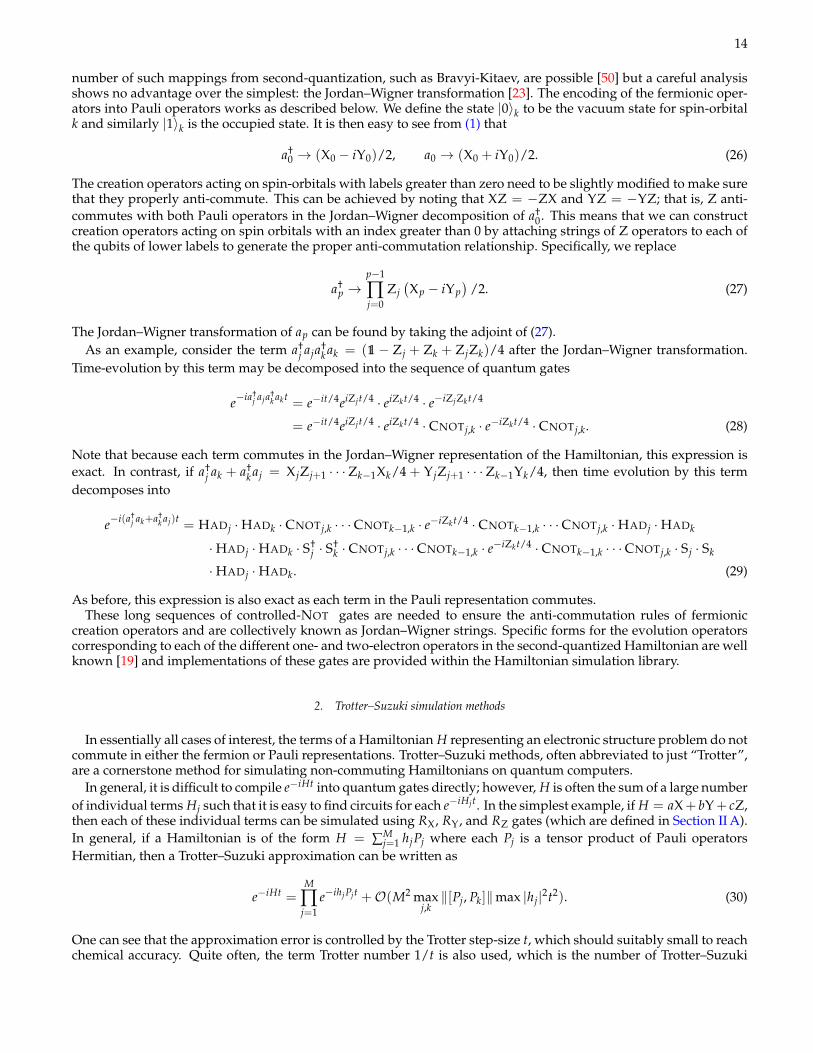
As before, this expression is also exact as each term in the Pauli representation commutes.These long sequences of controlled-NOT gates are needed to ensure the anti-commutation rules of fermionic

creation operators and are collectively known as Jordan–Wigner strings. Specific forms for the evolution operatorscorresponding to each of the different one- and two-electron operators in the second-quantized Hamiltonian are wellknown [19] and implementations of these gates are provided within the Hamiltonian simulation library.

2. Trotter–Suzuki simulation methods

In essentially all cases of interest, the terms of a Hamiltonian H representing an electronic structure problem do notcommute in either the fermion or Pauli representations. Trotter–Suzuki methods, often abbreviated to just “Trotter”,are a cornerstone method for simulating non-commuting Hamiltonians on quantum computers.

In general, it is difficult to compile e−iHt into quantum gates directly; however, H is often the sum of a large numberof individual terms Hj such that it is easy to find circuits for each e−iHjt. In the simplest example, if H = aX+ bY+ cZ,then each of these individual terms can be simulated using RX, RY, and RZ gates (which are defined in Section II A).In general, if a Hamiltonian is of the form H = ∑M

j=1 hjPj where each Pj is a tensor product of Pauli operatorsHermitian, then a Trotter–Suzuki approximation can be written as

e−iHt =M

∏j=1

e−ihjPjt +O(M2 maxj,k‖[Pj, Pk]‖max |hj|2t2). (30)

One can see that the approximation error is controlled by the Trotter step-size t, which should suitably small to reachchemical accuracy. Quite often, the term Trotter number 1/t is also used, which is the number of Trotter–Suzuki

15

formula applications required to achieve unit-time time-evolution. Furthermore, elementary quantum circuits in-volving chains only Clifford gates and a single qubit rotation can be used to simulate each exponential of a Paulioperator. Therefore, if the chemical Hamiltonian can be decomposed into a sum of a modest number of quantumcircuit is known to simulate e−iHt, then the Trotter formula can be used to build an approximation to e−iHt assum-ing t is sufficiently small. Using mappings such as Jordan–Wigner, fermion Hamiltonians are represented by as asum of Pauli operators, and methods exist for simulating such exponentials using a polynomial number of primitivequantum gates.

One example of a non-commuting fermion Hamiltonian is a combination of the terms from the previous section.Let H = a†

j aj + a†j ak + a†

k aj = (11− Zj)/2 + XjZj+1 · · · Zk−1Xk/4 + YjZj+1 · · · Zk−1Yk/4. A simulation circuit can beformulated using exactly the same methodology. However, because [Zk, Xk] 6= 0 6= [Zk, Yk] the error—often calledthe Trotter error—is O(t2) for such a simulation. Specifically, it can be shown using the same approach demonstratedabove that

e−iHt = e−it/2e−iZjt/2 ·HADj ·HADk · CNOTj,k · · ·CNOTk−1,k · e−iZkt/4 · CNOTk−1,k · · ·CNOTj,k ·HADj ·HADk

·HADj ·HADk · S†j · S†

k · CNOTj,k · · ·CNOTk−1,k · e−iZkt/4 · CNOTk−1,k · · ·CNOTj,k · Sj · Sk ·HADj ·HADk

+ O(M2 maxj,k‖[Hj, Hk]‖t2), (31)

Higher-order Trotter–Suzuki decompositions [10] also exist and are available within the Hamiltonian simulationlibrary. The simplest such decomposition is the symmetric (or second order) Trotter formula, which takes the form

e−iHt =M

∏j=1

e−iHjt/21

∏j=M

e−iHjt/2 + O(M3 maxj,k,`‖H`‖‖[Hj, Hk]‖t3). (32)

Arbitrarily high-order Trotter formulas can also be constructed from the second-order formula; however, the highest-order formula used in practice is the fourth-order formula [25].

Once e−iHt has been decomposed into a product of elementary unitary operations using one of the above formulas,we have everything that we need to simulate quantum dynamics on a quantum computer. However, for chemistrysimulation applications, we are usually interested in static properties like the correlation energy of a molecule. Ob-servables such as eigenvalues of the Hamiltonian can then be extracted from the time-evolution operator. For exam-ple, if H |ψ〉 = E |ψ〉 then e−iHt has eigenvalue e−iEt on the state. Thus, if we apply phase estimation on e−iHt, thenwe can learn Et directly from the phase and in turn E since t is known. For the purpose of estimating the ground-state eigenvalue, the second-order Trotter formula yields the same accuracy as the first-order Trotter formula, whichallows a potential savings of a factor of 2 in the complexity [22]. However, most simulation results use the symmetricformula to simplify the error analysis.

In theory, this simulation approach does not compare favorably asymptotically to methods based on qubitizationor linear combinations of unitaries; however, Trotter–Suzuki formulas require fewer qubits than any other knownmethod. Moreover, the complexity of the simulation depends strongly on the size of the commutators between theHamiltonian terms. In practice, this means that Trotter–Suzuki methods can be more efficient than more recent sim-ulation methods for some problems [25] and, therefore, will remain an important part of the landscape of quantumsimulation algorithms for the foreseeable future.

3. Qubitization simulation methods

In the previous section, we described the Trotter–Suzuki algorithm that directly approximates the unitary time-evolution operator e−iHt. However, for the purposes of estimating eigenvalues of the Hamiltonian H, it sufficesto implement time-evolution by any monotonic function of H, say ei f (H), where f (·) is applied to the eigenvaluesof H without modifying the eigenvectors [51, 52]. Qubitization [14] is a simulation technique for synthesizing aunitary that is exactly ei sin−1(H/h) for some normalization constant h ≥ ‖H‖, up to fixed phase factors and localisometries. Compared to the Trotter–Suzuki algorithm, qubitization offers a different complexity tradeoff that maybe advantageous in certain situations.

The starting point of qubitization is a Hamiltonian represented as a linear combination of N Pauli operators Pjwith positive coefficients hj, say

H =N

∑j=0

hjPj. (33)

16

Such a decomposition can be found for the chemistry Hamiltonian by using the Jordan–Wigner decomposition givenin (27). Information about this Hamiltonian is then encoded in two unitary operators PREPARE and SELECT. Coeffi-cient information is encoded in a quantum state

|h〉 =N−1

∑j=0

√|hj|h|j〉 , (34)

where h = ∑N−1j=0 |hj| is the one-norm of coefficients. Note that the number state |j〉 encodes a binary representation

of j, e.g. |6〉 = |1〉 |1〉 |0〉. This state can be prepared by the quantum circuit

PREPARE |0〉 = |h〉 , (35)

implemented following Ref. [53]. Operator information is encoded in a unitary operator, implemented followingRef. [26],

SELECT =N−1

∑j=0|j〉 〈j| ⊗ Pj, (36)

that applies the jth Pauli operator given the number state |j〉. Together, these combine to apply the Hamiltonian inthe sense of

V = (PREPARE† ⊗ 1) · SELECT · (PREPARE⊗ 1) (37)Hh

= (〈0| ⊗ 1) ·V · (|0〉 ⊗ 1).

By combining PREPARE and SELECT, qubitization is simply the walk operator

W = ((2 |0〉 〈0| − 1)⊗ 1) ·V. (38)

When evaluating its action on eigenstates |E〉 of H |E〉 = E |E〉 with energy E when the input in the other register is|0〉, there are two cases of interest: |E| = h, and |E| 6= h. In the former case,

W |0〉 |E〉 = Eh|0〉 |E〉 = sign[E] |0〉 |E〉 . (39)

Thus, the walk operator simply applies a phase 0 or π to the input. In the latter case, using the simplified notationEh = λ,

W |0〉 |E〉 = λ |0〉 |E〉 −√

1− |λ|2 |0E⊥〉 , (40)

where |0E⊥〉 is orthogonal to the original input. By rearranging, this new state

|0E⊥〉 = −W |0〉 |E〉+ λ |0〉 |E〉√1− |λ|2

. (41)

Thus, we may evaluate the matrix elements of W in this basis as

W =⊕

E

[E/h

√1− |E/h2

−√

1− |E/h2 E/h

]. (42)

By diagonalizing each subspace separately, we see that W applies a phase e∓i cos−1 (E/h) to the eigenstates |0〉|E〉±|0E⊥〉√2

.Within this basis, the spectrum of the walk operator is isomorphic to

W = e−iY⊗cos−1(H/h) = −ie−iY⊗sin−1(H/h). (43)

17

4. Circuit optimizations for qubitization

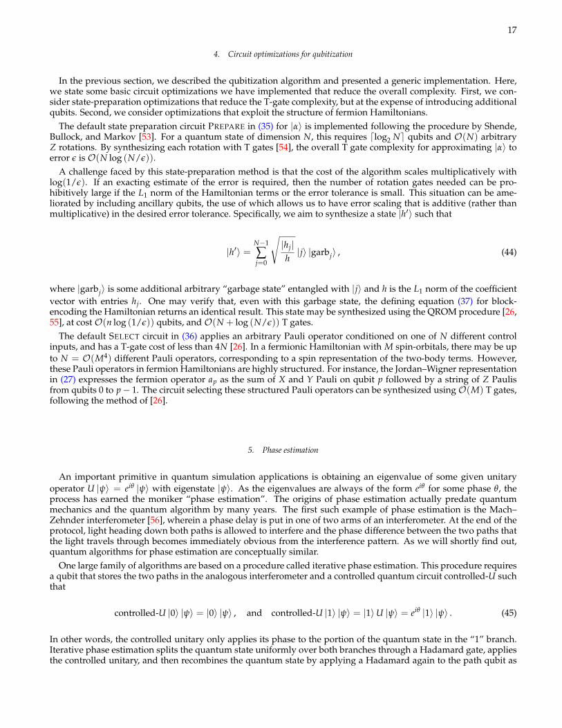
In the previous section, we described the qubitization algorithm and presented a generic implementation. Here,we state some basic circuit optimizations we have implemented that reduce the overall complexity. First, we con-sider state-preparation optimizations that reduce the T-gate complexity, but at the expense of introducing additionalqubits. Second, we consider optimizations that exploit the structure of fermion Hamiltonians.

The default state preparation circuit PREPARE in (35) for |α〉 is implemented following the procedure by Shende,Bullock, and Markov [53]. For a quantum state of dimension N, this requires dlog2 Ne qubits and O(N) arbitraryZ rotations. By synthesizing each rotation with T gates [54], the overall T gate complexity for approximating |α〉 toerror ε is O(N log (N/ε)).

A challenge faced by this state-preparation method is that the cost of the algorithm scales multiplicatively withlog(1/ε). If an exacting estimate of the error is required, then the number of rotation gates needed can be pro-hibitively large if the L1 norm of the Hamiltonian terms or the error tolerance is small. This situation can be ame-liorated by including ancillary qubits, the use of which allows us to have error scaling that is additive (rather thanmultiplicative) in the desired error tolerance. Specifically, we aim to synthesize a state |h′〉 such that

|h′〉 =N−1

∑j=0

√|hj|h|j〉 |garbj〉 , (44)

where |garbj〉 is some additional arbitrary “garbage state” entangled with |j〉 and h is the L1 norm of the coefficientvector with entries hj. One may verify that, even with this garbage state, the defining equation (37) for block-encoding the Hamiltonian returns an identical result. This state may be synthesized using the QROM procedure [26,55], at cost O(n log (1/ε)) qubits, and O(N + log (N/ε)) T gates.

The default SELECT circuit in (36) applies an arbitrary Pauli operator conditioned on one of N different controlinputs, and has a T-gate cost of less than 4N [26]. In a fermionic Hamiltonian with M spin-orbitals, there may be upto N = O(M4) different Pauli operators, corresponding to a spin representation of the two-body terms. However,these Pauli operators in fermion Hamiltonians are highly structured. For instance, the Jordan–Wigner representationin (27) expresses the fermion operator ap as the sum of X and Y Pauli on qubit p followed by a string of Z Paulisfrom qubits 0 to p− 1. The circuit selecting these structured Pauli operators can be synthesized using O(M) T gates,following the method of [26].

5. Phase estimation

An important primitive in quantum simulation applications is obtaining an eigenvalue of some given unitaryoperator U |ψ〉 = eiθ |ψ〉 with eigenstate |ψ〉. As the eigenvalues are always of the form eiθ for some phase θ, theprocess has earned the moniker “phase estimation”. The origins of phase estimation actually predate quantummechanics and the quantum algorithm by many years. The first such example of phase estimation is the Mach–Zehnder interferometer [56], wherein a phase delay is put in one of two arms of an interferometer. At the end of theprotocol, light heading down both paths is allowed to interfere and the phase difference between the two paths thatthe light travels through becomes immediately obvious from the interference pattern. As we will shortly find out,quantum algorithms for phase estimation are conceptually similar.

One large family of algorithms are based on a procedure called iterative phase estimation. This procedure requiresa qubit that stores the two paths in the analogous interferometer and a controlled quantum circuit controlled-U suchthat

controlled-U |0〉 |ψ〉 = |0〉 |ψ〉 , and controlled-U |1〉 |ψ〉 = |1〉U |ψ〉 = eiθ |1〉 |ψ〉 . (45)

In other words, the controlled unitary only applies its phase to the portion of the quantum state in the “1” branch.Iterative phase estimation splits the quantum state uniformly over both branches through a Hadamard gate, appliesthe controlled unitary, and then recombines the quantum state by applying a Hadamard again to the path qubit as

18

follows.

|0〉 |ψ〉 7→ 1√2(|0〉 |ψ〉+ |1〉 |ψ〉)

7→ 1√2

(|0〉 |ψ〉+ eiθ |1〉 |ψ〉

)7→ 1

2

((1 + eiθ) |0〉 |ψ〉+ (1− eiθ) |1〉 |ψ〉

)= eiθ/2 (cos(θ/2) |0〉 |ψ〉 − i sin(θ/2) |1〉 |ψ〉) (46)

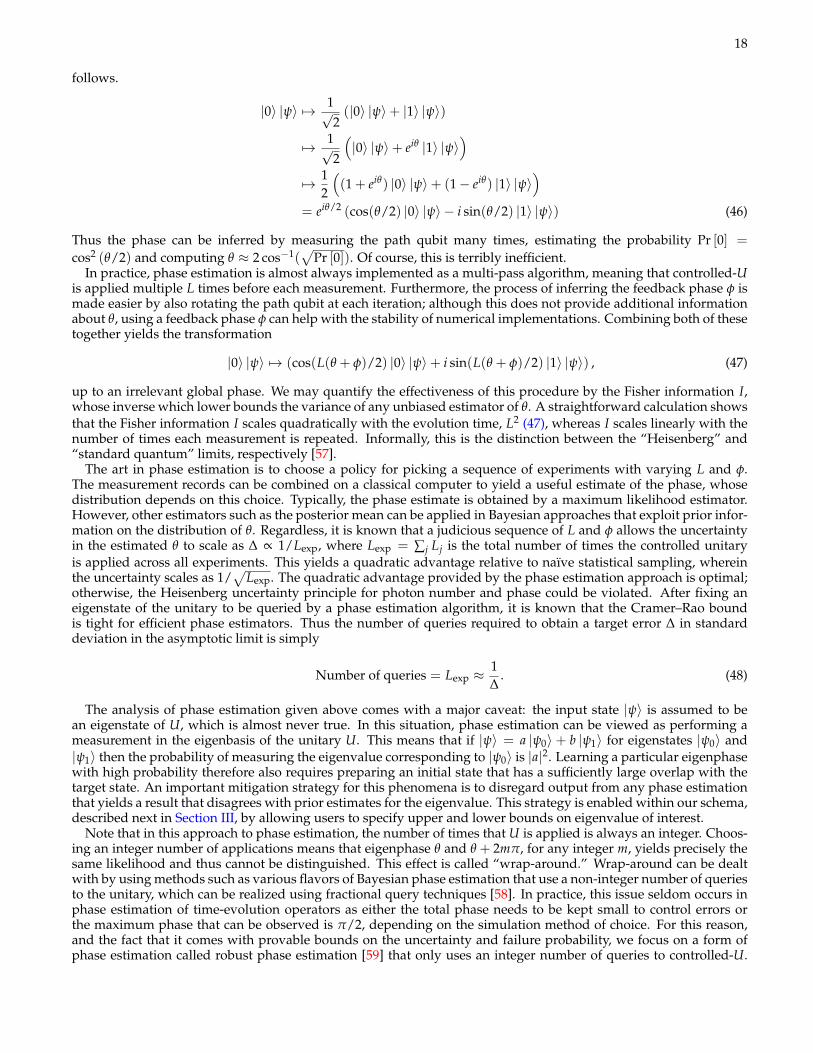
Thus the phase can be inferred by measuring the path qubit many times, estimating the probability Pr [0] =

cos2 (θ/2) and computing θ ≈ 2 cos−1(√

Pr [0]). Of course, this is terribly inefficient.In practice, phase estimation is almost always implemented as a multi-pass algorithm, meaning that controlled-U

is applied multiple L times before each measurement. Furthermore, the process of inferring the feedback phase φ ismade easier by also rotating the path qubit at each iteration; although this does not provide additional informationabout θ, using a feedback phase φ can help with the stability of numerical implementations. Combining both of thesetogether yields the transformation

|0〉 |ψ〉 7→ (cos(L(θ + φ)/2) |0〉 |ψ〉+ i sin(L(θ + φ)/2) |1〉 |ψ〉) , (47)

up to an irrelevant global phase. We may quantify the effectiveness of this procedure by the Fisher information I,whose inverse which lower bounds the variance of any unbiased estimator of θ. A straightforward calculation showsthat the Fisher information I scales quadratically with the evolution time, L2 (47), whereas I scales linearly with thenumber of times each measurement is repeated. Informally, this is the distinction between the “Heisenberg” and“standard quantum” limits, respectively [57].

The art in phase estimation is to choose a policy for picking a sequence of experiments with varying L and φ.The measurement records can be combined on a classical computer to yield a useful estimate of the phase, whosedistribution depends on this choice. Typically, the phase estimate is obtained by a maximum likelihood estimator.However, other estimators such as the posterior mean can be applied in Bayesian approaches that exploit prior infor-mation on the distribution of θ. Regardless, it is known that a judicious sequence of L and φ allows the uncertaintyin the estimated θ to scale as ∆ ∝ 1/Lexp, where Lexp = ∑j Lj is the total number of times the controlled unitaryis applied across all experiments. This yields a quadratic advantage relative to naïve statistical sampling, whereinthe uncertainty scales as 1/

√Lexp. The quadratic advantage provided by the phase estimation approach is optimal;

otherwise, the Heisenberg uncertainty principle for photon number and phase could be violated. After fixing aneigenstate of the unitary to be queried by a phase estimation algorithm, it is known that the Cramer–Rao boundis tight for efficient phase estimators. Thus the number of queries required to obtain a target error ∆ in standarddeviation in the asymptotic limit is simply

Number of queries = Lexp ≈1∆

. (48)

The analysis of phase estimation given above comes with a major caveat: the input state |ψ〉 is assumed to bean eigenstate of U, which is almost never true. In this situation, phase estimation can be viewed as performing ameasurement in the eigenbasis of the unitary U. This means that if |ψ〉 = a |ψ0〉 + b |ψ1〉 for eigenstates |ψ0〉 and|ψ1〉 then the probability of measuring the eigenvalue corresponding to |ψ0〉 is |a|2. Learning a particular eigenphasewith high probability therefore also requires preparing an initial state that has a sufficiently large overlap with thetarget state. An important mitigation strategy for this phenomena is to disregard output from any phase estimationthat yields a result that disagrees with prior estimates for the eigenvalue. This strategy is enabled within our schema,described next in Section III, by allowing users to specify upper and lower bounds on eigenvalue of interest.

Note that in this approach to phase estimation, the number of times that U is applied is always an integer. Choos-ing an integer number of applications means that eigenphase θ and θ + 2mπ, for any integer m, yields precisely thesame likelihood and thus cannot be distinguished. This effect is called “wrap-around.” Wrap-around can be dealtwith by using methods such as various flavors of Bayesian phase estimation that use a non-integer number of queriesto the unitary, which can be realized using fractional query techniques [58]. In practice, this issue seldom occurs inphase estimation of time-evolution operators as either the total phase needs to be kept small to control errors orthe maximum phase that can be observed is π/2, depending on the simulation method of choice. For this reason,and the fact that it comes with provable bounds on the uncertainty and failure probability, we focus on a form ofphase estimation called robust phase estimation [59] that only uses an integer number of queries to controlled-U.

19

Other algorithms exist and we recommend the interested reader to look at faster phase estimation [60], Bayesianphase estimation [61], and quantum phase estimation [4]. Each of these approaches has different tradeoffs betweenexperimental run time, classical processing, and the number of quantum bits used in the protocol.

III. THE BROOMBRIDGE SCHEMA FOR REPRESENTING ELECTRONIC STRUCTURE PROBLEMS

The Broombridge schema1 defines a data structure for representing electronic structure problems together withsupporting metadata to enable effective simulation on a quantum computer. Using a human-readable serialization,this provides an interface between electronic structure calculation tools, in particular NWChem, and the MicrosoftQuantum Development Kit chemistry library. By standardizing this interface under the open-source MIT license,we also enable potential inter-operation between any set of classical and quantum chemistry simulation softwarepackages, and enable future schema extensions to meet the requirements of state-of-the-art electronic structure algo-rithms.

We outline in Section III A the essential components contained in Broombridge that are relevant to the chemistrylibrary. Subsequently, we describe in Section III B how Broombridge may be generated by NWChem, which is usedlater in the examples of Section V.

A. Broombridge v0.1 specifications

We now present snippets from the Broombridge example of LiH that highlight its essential keys and values. Asfuture versions of Broombridge may not be backwards-compatible, each Broombridge instance begins with a versionnumber and a link to its specification. Some entries of Broombridge are required and will not pass validation ifomitted, whereas other entries are optional metadata, as shown in the following Listing 8.

1 # ( Required ) Address to complete d e f i n i t i o n f o r va l ida ing Broombridge v0 . 1 ."$schema": https://raw.githubusercontent.com/Microsoft/Quantum/master/Chemistry/Schema/broombridge-0.1.

↪→ schema.json

# ( Required ) Broombridge vers ion of e l e c t r o n i c s t r u c t u r e problem r e p r e s e n t a t i o n .format: {version: ’0.1’}

6

# ( Optional ) Bibl iography f o r problems represented in t h i s Broombridge .bibliography:- url: ’https://www.nwchem-sw.org’

Listing 8. Broombridge version number formatting. examples/lih.yaml

A quantitative description of the electronic structure problem is stored as an entry in the ‘integral_set’ list – mul-tiple Broombridge problems may be stored in this list. Each entry in this list contains a description of the problem.Some parameters are essential for specifying a complete quantum simulation problem. This includes the numberof orbitals and electrons required, the constant energy offsets equivalent to identify terms in the Hamiltonian, theHartree–Fock energy, and the one-electron and two-electron integrals over the defined orbital subspace. These areoutlined in the following Listing 9.

1 # Terms in the e l e c t r o n i c s t r u c t u r e Hamiltonian .hamiltonian:# L i s t of one−e l e c t r o n i n t e g r a l sone_electron_integrals:

# Only non−zero terms are s p e c i f i e d in a sparse format .6 format: sparse

units: hartreevalues:# Each element [ i , j , hij ] , where i, j ∈ {1, · · · ,n_orbitals} , i s the o r b i t a l i n t e g r a l (12) .# As hij = hji , only one of these terms must be s p e c i f i e d .

11 - [1, 1, -4.7225445389]- [2, 1, 0.1046509472]# e t c .

1 So named after the Broom bridge in Dublin, Ireland, upon which Sir William Rowan Hamilton, the namesake of ‘Hamiltonian’, inscribed thefirst defining equations of quarternions.

20

# L i s t of two−e l e c t r o n i n t e g r a l s16 two_electron_integrals:

format: sparseindex_convention: mullikenunits: hartreevalues:

21 # Each element [ i , l , j , k , hijkl ] , where i, j, j, k ∈ {1, · · · ,n_orbitals} , i s the o r b i t a l i n t e g r a l (13) .# As hijkl = hjilk = hikjl = hlkji f o r r e a l o r b i t a l s , only one of these terms must be s p e c i f i e d .- [1, 1, 1, 1, 1.6586341297]- [2, 1, 1, 1, -0.110636355]# e t c .

Listing 9. Essential Broombridge components for specifying an electronic structure problem. examples/lih.yaml

Some elements of this description are optional but are highly recommended as they can be used by the chemistrylibrary. Importantly, as shown in Listing 10, this includes multi-configurational trial wavefunctions that are super-positions of Slater determinants, as well as approximations to the full configuration-interaction energy that can alsobe used to determine the principle range of phase estimation, if applicable.

# Approximate upper and lower bounds on the exac t ground−s t a t e energy .fci_energy: {units: hartree, lower: -7.981844675840114, upper: -7.781844675840115}

# Various multi−c o n f i g u r a t i o n a l t r i a l wavefunctions .5 initial_state_suggestions:

# This i s a ground s t a t e t r i a l wavefunction .- state:

# Approximate energy of t h i s s t a t e10 energy: {units: hartree, value: -7.881844675840115}

# Label used to r e f e r e n c e t h i s s t a t e .label: ’|G>’

15 # The t r i a l wavefunction descr ibed by a superpos i t ion where each entry i s the amplitude followed# by the corresponding S l a t e r determininant descr ibed by fermion operators a c t i n g on the vacuum# s t a t e . In Pol i sh notat ion , (3 a ) +≡ a†

3,↑ , ( 2 b )≡ a2,↓ , ( 2 a )≡ a2,↑ and so on .superposition:- [0.993182561322233, (1a)+, (2a)+, (1b)+, (2b)+, ’|vacuum>’]

20 - [-0.116569292206005, (6a)+, (6b)+, (2b), (2a), (1a)+, (2a)+, (1b)+, (2b)+, ’|vacuum>’]

# This i s a f i r s t e x c i t e d s t a t e t r i a l wavefunction .- state:

energy: {units: hartree, value: -7.750219591632256}25 label: ’|E1>’

superposition:- [0.664745837968804, (3a)+, (2a), (1a)+, (2a)+, (1b)+, (2b)+, ’|vacuum>’]- [0.664745837968804, (3b)+, (2b), (1a)+, (2a)+, (1b)+, (2b)+, ’|vacuum>’]- [-0.246552630006247, (3a)+, (3b)+, (2b), (2a), (1a)+, (2a)+, (1b)+, (2b)+, ’|vacuum>’]

30 - [0.166489853209298, (3a)+, (6b)+, (2b), (2a), (1a)+, (2a)+, (1b)+, (2b)+, ’|vacuum>’]

Listing 10. Recommended Broombridge properties that can be used by the chemistry library. examples/lih.yaml

Some elements of this description are optional and are not currently used by the chemistry library. For instance,this includes the molecule geometry and the basis set as outlined in the following Listing 11. Full details of allother fields are documented online at https://docs.microsoft.com/en-us/quantum/libraries/chemistry/schema/broombridge.

# Bas i s s e t used to represent problem .2 basis_set: {name: sto-3g, type: gaussian}

# Geometry descr ib ing the problem .geometry:

atoms:7 - {name: Li, coords: [0.0, 0.0, -0.406]}

- {name: H, coords: [0.0, 0.0, 1.218]}coordinate_system: cartesiansymmetry: c1units: angstrom

21

12

# Any a d d i t i o n a l miscel laneous metadata . This must be included , but may be empty .metadata: {}

Listing 11. Select optional Broombridge properties not used by the chemistry library. examples/lih.yaml

B. Generating Broombridge with NWChem

One of the following methods may be used to either obtain or generate a description of an electronic structureproblem, serialized as Broombridge.

• The easiest way to obtain Broombridge is from the numerous existing samples at, say, https://github.com/Microsoft/Quantum/tree/master/Chemistry/IntegralData/YAML.

• The next easiest way to generate Broombridge is to use the EMSL Arrows Builder for the Microsoft Quan-tum Development Kit at https://arrows.emsl.pnnl.gov/api/qsharp_chem. This is a web-based frontend toNWChem and chemical computational databases for many materials and chemical modeling problems viaa broad spectrum of digital communications, including posts to web API. With this framework, a moleculecan be input into EMSL Arrows using a variety of techniques documented at http://www.nwchem-sw.org/index.php/EMSL_Arrows say, the simplified molecular-input line-entry system, a graphical 2D or 3D moleculebuilder, or as a standard NWChem input deck.

• For the most flexibility, PNNL also provides a Docker image that automatically compiles a virtual machinecontaining a complete and executable version of NWChem.

• An advanced user may also download and compile NWChem from source.

Broombridge is obtained by serializing the output file dump of an NWChem computation of the format outlinedin Section II B 2, using the Python script provided with NWChem. A convenient frontend to the Docker image forNWChem is provided with the Quantum Development Kit as a cross-platform PowerShell script.

IV. SIMULATING QUANTUM CHEMISTRY WITH THE MICROSOFT QUANTUM DEVELOPMENT KIT

The Microsoft Quantum Development Kit chemistry library implements the quantum simulation algorithmsof Section II C in Q# with chemistry-specific optimizations, and provides an interface in C# to define fermion Hamil-tonians relevant to chemistry, such as through the Broombridge schema in Section III. Taken together, a quantumsimulation of any electronic structure problem generated by NWChem in Section III B may be executed on any thetarget machine provided by the Microsoft Quantum Development Kit. The two target machines relevant here are:(1) the full-state simulator, which emulates a noiseless quantum computer, albeit with exponential time scaling inqubit count, and (2) the trace simulator, which evaluates various resource costs of the simulation with polynomialtime scaling in qubit count.

We describe use of this library through a quantum simulation of molecular hydrogen. In Section IV A, we constructthe hydrogen Hamiltonian, and simulate its real-time evolution. Real-time evolution is then invoked as a subroutineto obtain estimates of the ground-state energy in Section IV C. For molecules with many qubits, full-state simulationon a classical machine is intractable. However, efficiently obtaining cost estimates of the simulation is possible simplyby swapping in the trace simulator.

A. Constructing qubit Hamiltonians from chemistry Hamiltonians

Consider a simple representation of molecular hydrogen in the STO-3G with two orbitals. In this basis, the hydro-gen Hamiltonian has the form

H = h0 I + ∑i,j

hi,j ∑σ∈{↑,↓}

a†i,σaj,σ +

12 ∑

i,j,k,lhi,j,k,l ∑

σ,ρ∈{↑,↓}a†

i,σa†j,ρak,ρal,σ, (49)

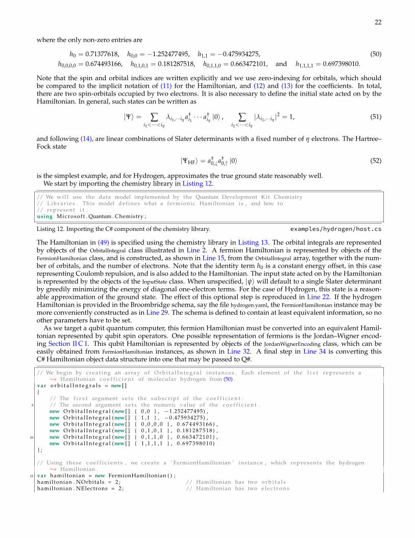
22

where the only non-zero entries are

h0 = 0.71377618, h0,0 = −1.252477495, h1,1 = −0.475934275, (50)h0,0,0,0 = 0.674493166, h0,1,0,1 = 0.181287518, h0,1,1,0 = 0.663472101, and h1,1,1,1 = 0.697398010.

Note that the spin and orbital indices are written explicitly and we use zero-indexing for orbitals, which shouldbe compared to the implicit notation of (11) for the Hamiltonian, and (12) and (13) for the coefficients. In total,there are two spin-orbitals occupied by two electrons. It is also necessary to define the initial state acted on by theHamiltonian. In general, such states can be written as

|Ψ〉 = ∑i1<···<iη

λi1,···iη a†i1 · · · a

†iη |0〉 , ∑

i1<···<iη

|λi1,···iη |2 = 1, (51)

and following (14), are linear combinations of Slater determinants with a fixed number of η electrons. The Hartree–Fock state

|ΨHF〉 = a†0,↓a

†0,↑ |0〉 (52)

is the simplest example, and for Hydrogen, approximates the true ground state reasonably well.We start by importing the chemistry library in Listing 12.

// We w i l l use the data model implemented by the Quantum Development Kit Chemistry// L i b r a r i e s . This model de f ines what a fermionic Hamiltonian is , and how to// represent i t .using Microsof t . Quantum . Chemistry ;

Listing 12. Importing the C# component of the chemistry library. examples/hydrogen/host.cs

The Hamiltonian in (49) is specified using the chemistry library in Listing 13. The orbital integrals are representedby objects of the OrbitalIntegral class illustrated in Line 2. A fermion Hamiltonian is represented by objects of theFermionHamiltonian class, and is constructed, as shown in Line 15, from the OrbitalIntegral array, together with the num-ber of orbitals, and the number of electrons. Note that the identity term h0 is a constant energy offset, in this caserepresenting Coulomb repulsion, and is also added to the Hamiltonian. The input state acted on by the Hamiltonianis represented by the objects of the InputState class. When unspecified, |ψ〉 will default to a single Slater determinantby greedily minimizing the energy of diagonal one-electron terms. For the case of Hydrogen, this state is a reason-able approximation of the ground state. The effect of this optional step is reproduced in Line 22. If the hydrogenHamiltonian is provided in the Broombridge schema, say the file hydrogen.yaml, the FermionHamiltonian instance may bemore conveniently constructed as in Line 29. The schema is defined to contain at least equivalent information, so noother parameters have to be set.

As we target a qubit quantum computer, this fermion Hamiltonian must be converted into an equivalent Hamil-tonian represented by qubit spin operators. One possible representation of fermions is the Jordan–Wigner encod-ing Section II C 1. This qubit Hamiltonian is represented by objects of the JordanWignerEncoding class, which can beeasily obtained from FermionHamiltonian instances, as shown in Line 32. A final step in Line 34 is converting thisC# Hamiltonian object data structure into one that may be passed to Q#.

// We begin by c r e a t i n g an array of O r b i t a l I n t e g r a l i n s t a n c e s . Each element of the l i s t r e p r e s e n t s a↪→ Hamiltonian c o e f f i c i e n t of molecular hydrogen from (50) .

var o r b i t a l I n t e g r a l s = new [ ]{

// The f i r s t argument s e t s the s u b s c r i p t of the c o e f f i c i e n t .5 // The second argument s e t s the numeric value of the c o e f f i c i e n t .

new O r b i t a l I n t e g r a l (new [ ] { 0 ,0 } , −1.252477495) ,new O r b i t a l I n t e g r a l (new [ ] { 1 ,1 } , −0.475934275) ,new O r b i t a l I n t e g r a l (new [ ] { 0 , 0 , 0 , 0 } , 0 .674493166 ) ,new O r b i t a l I n t e g r a l (new [ ] { 0 , 1 , 0 , 1 } , 0 .181287518 ) ,

10 new O r b i t a l I n t e g r a l (new [ ] { 0 , 1 , 1 , 0 } , 0 .663472101 ) ,new O r b i t a l I n t e g r a l (new [ ] { 1 , 1 , 1 , 1 } , 0 .697398010 )

} ;

// Using these c o e f f i c i e n t s , we c r e a t e a ‘ FermionHamiltonian ’ ins tance , which r e p r e s e n t s the hydrogen↪→ Hamiltonian .

15 var hamiltonian = new FermionHamiltonian ( ) ;hamiltonian . NOrbitals = 2 ; // Hamiltonian has two o r b i t a l shamiltonian . NElectrons = 2 ; // Hamiltonian has two e l e c t r o n s

23

hamiltonian . EnergyOffset = 0 . 7 1 3 7 7 6 1 8 ; // I d e n t i t y term in the Hamiltonian .hamiltonian . AddFermionTerm ( o r b i t a l I n t e g r a l s ) ; // Add a l l o r b i t a l i n t e g r a l s .

20

// We then s e l e c t the s i n g l e S l a t e r determinant input s t a t e of the Hamiltonian , which i s the d e f a u l t↪→ choice .

var i n p u t S t a t e = hamiltonian . GreedyStatePreparat ion ( ) ;// Input s t a t e s are given a l a b e l to i d e n t i t f y then l a t e r on . The d e f a u l t has the l a b e l " Greedy " .var inputSta teChoice = i n p u t S t a t e . Label ;

25 // Assign t h i s s t a t e to the ‘ FermionHamiltonian ’ i n s t a n c e . The choice of which s t a t e from the l i s t to↪→ prepare in the quantum algorithm may be made l a t e r .

hamiltonian . I n p u t S t a t e s = new Lis t <FermionHamiltonian . InputState > ( ) { i n p u t S t a t e } ;

// A l t e r n a t v i e l y , we can c r e a t e a l i s t of ‘ FermionHamiltonian ’ i n s t a n c e s from a s i n g l e Broombridge f i l e ,↪→ which may conta in d e s c r i p t i o n s of mult ip le Hamiltonians .

var hamiltoniansFromBroombridge = FermionHamiltonian . LoadFromYAML( " hydrogen . yaml " ) ;30

// The Jordan−Wigner encoding converts the fermion Hamiltonian , expressed in terms of fermionic operators ,↪→ to a qubit Hamiltonian , expressed in terms of Paul i matr ices . This i s an e s s e n t i a l s tep f o r↪→ s imulat ing our constructed Hamiltonians on a qubit quantum computer .

var jordanWignerEncoding = JordanWignerEncoding . Create ( hamiltonian ) ;// Converts jordanWignerEncoding i n t o format consumable by Q# . This d e f a u l t s to " Greedy " i f the opt iona l

↪→ argument ‘ inputStateChoice ‘ i s not provided .var qSharpData = jordanWignerEncoding . QSharpData ( inputSta teChoice ) ;

Listing 13. Specifying a Hydrogen Hamiltonian in the chemistry library. examples/hydrogen/host.cs

B. Synthesizing quantum simulation circuits

The quantum simulation algorithms of Trotter–Suzuki and Qubitization are implemented in the Q# canon libraryof the Microsoft Quantum Development Kit. The chemistry library provides an interface to invoke these algorithmsusing the C# Hamiltonian data structures of the previous section. In this section, we use the chemistry library toobtain operations representing preparation of the initial quantum state, and dynamical evolution by these Hamilto-nians. We start by importing the Q# component of the chemistry library as follows.

// Imports Q# components of the chemistry l i b r a r y f o r the Jordan−Wigner encoding .open Microsof t . Quantum . Chemistry . JordanWigner ;

// Import the math constant π and the r e a l modulus funct ion .5 open Microsof t . Quantum . Extensions . Math

Listing 14. Importing the Q# component of the chemistry library. examples/hydrogen/hydrogen.qs

As the required number of qubits depends on the choice of quantum simulation algorithm, this information is alsoreturned by the chemistry library. The results of these steps, illustrated in Listing 15, are used to obtain eigenstateenergy estimates in the next section. In Line 7, we deconstruct the qSharpData data structure, representing hydrogen,from the previous section into components to be processed in Q#.

We consider two simulation techniques. First, in Line 9, we use the chemistry library to synthesize an operationthat implements a single step of the Trotter–Suzuki integrator. The integrator order is set in Line 11. This circuitapproximates real-time evolution e−iHt, where t is the integrator step size, set in Line 13. Second, in Line 24, weinstead synthesize an operation that implements a quantum walk by H using the Qubitization procedure. Thisquantum walk implements the unitary with spectrum similar to eiY⊗sin−1(H/h), which may be understood as time-evolution by the Hamiltonian, but with a modified spectrum. Note that h is the L1 norm of the Hamiltonian termcoefficients. An operation that synthesizes the ‘‘ Greedy’’ input state, specified in the previous section is obtainedin Line 32.

//The Q# data s t r u c t u r e ‘ qSharpData ‘ from Line 34 of Listing 13 r e p r e s e n t s hydrogen .// This decons t ruc ts i n t o v a r i a b l e s t h a t w i l l be passed to l a t e r Q# algori thms .// ‘ nSpinOrbita ls ‘ i s the number of spin−o r b i t a l s .// ‘ data ‘ d e s c r i b e s Hamiltonian terms .

5 // ‘ statePrepData ‘ d e s c r i b e s the input s t a t e the s imulat ion algorithm a c t s on .// ‘ energyOffset ‘ i s the i d e n t i t y c o e f f i c i e n t of the Hamiltonian .l e t ( nSpinOrbi ta ls , data , statePrepData , energyOffset ) = qSharpData ! ;

// Using T r o t t e r i z a t i o n //////////////////////////////////////////////////

24

10 // Set the Trot te r−−Suzuki i n t e g r a t i o n order .l e t order = 1 ;// Set the Trot te r−−Suzuki i n t e g r a t i o n step s i z e .l e t s t e p S i z e = 0 . 4 ;

15 // Apply the chemistry l i b r a r y funct ion ‘ Trot terS tepOrac le ‘ to the Q#// data s t r u c t u r e r e p r e s e n t a t i n g hydrogen .// ‘ nQubits ‘ i s the number of qubi t s a l l o c a t e d to the quantum c i r c u i t .// ‘ r e s c a l e ‘ i s ‘ 1 .0/ t r o t t e r S t e p S i z e ‘ , and i s the number of T r o t t e r s teps// needed to s imulat ion evolut ion f o r uni t time .

20 // ‘ t r o t t e r S t e p ‘ i s an operat ion implenting one Trot te r−−Suzuki s tep .l e t ( nQubits , ( r e s c a l e , t r o t t e r S t e p ) ) =

T r o t t e r S t e p O r a c l e ( qSharpData , s tepSize , order ) ;

// Using Qubi t iza t ion ////////////////////////////////////////////////////25 // Apply the chemistry l i b r a r y funct ion ‘ Qubi t izat ionOrac le ‘ to the Q#

// data s t r u c t u r e r e p r e s e n t a t i n g hydrogen .// ‘ nQubits ‘ i s the number of qubi t s a l l o c a t e d to the quantum c i r c u i t .// ‘ r e s c a l e ‘ i s the L1 norm of Hamiltonian c o e f f i c i e n t s .// ‘quantumWalk ‘ i s an operat ion implenting one quantum walk step .

30 l e t ( nQubits , ( l1Norm , quantumWalk ) ) = Qubi t iza t ionOrac le ( qSharpData ) ;

// S t a t e Preparat ion /////////////////////////////////////////////////////// Apply the chemistry l i b r a r y operat ion ‘ P r e p a r e T r i a l S t a t e ‘ to// synthes ize a quantum c i r c u i t t h a t prepares the i n i t i a l s t a t e acted on by

35 // the Hamiltonian . Note t h a t the p a r t i a l a p p l i c a t i o n of the l a s t paramter ,// which has the ‘ Qubit [ ] ‘ type .l e t s t a t e P r e p = P r e p a r e T r i a l S t a t e ( statePrepData , _ ) ;

Listing 15. Quantum simulation circuits by the Hamiltonian in Listing 13. examples/hydrogen/hydrogen.qs

C. Estimating eigenvalues

The operations we assembled in the previous section simulate quantum dynamics. These operations may becombined with phase estimation—described in Section II C 5—to estimate energy levels En of the Hamiltonian. Ifthe code from Listing 15 is used to specify the approximation to e−iHt and the initial state, then the application ofphase estimation here will provide an estimate of the ground-state energy of hydrogen with high probability becauseof the large overlap between the ground-state of hydrogen and the Hartree–Fock trial state used therein.

Below in Listing 16, we illustrate this procedure by combining the chemistry library with phase estimation in thecanon library. Specifically, we apply robust phase estimation below to estimate an eigenvalue of the Hamiltonian.

// Choose robust phase es t imat ion amongst various p o s s i b l e phase// es t imat ion algori thms in the Q# canon . This i s parameterized by b i t s

3 // of p r e c i s i o n ‘b ‘ which c o n t r o l s the standard devia t ion ≈ 2b−1 of// the returned phase .l e t n B i t s = 8 ;l e t phaseEstAlg = RobustPhaseEstimation ( nBits , _ , _ ) ;

8 // Use the Q# canon funct ion ‘ EstimateEnergy ‘ t h a t a l l o c a t e s qubi t s// to the quantum simulat ion , c r e a t e s the input s t a t e s , performs// phase est imat ion , and then re turns the est imated phase .l e t phaseEst = EstimateEnergy ( nQubits , s ta tePrep , t r o t t e r S t e p , phaseEstAlg ) ;

13 // Rescale the est imated phase to obta in the energy , and a l s o add the// i d e n t i t y c o e f f i c i e n t of the Hamiltonian .l e t energyEst = phaseEst * r e s c a l e + energyOffset ;

// Suppose a guess of the true energy i s a v a i l a b l e to i d e n t i f y the p r i n c i p l e value18 // range .

l e t energyGuess = −1.0;

// Add the mul t ip les of 2π to obta in the p r i n c i p l e value using// the canon ‘RealMod ‘ modulus funct ion .

23 l e t pr inc ip leEnergyEst =RealMod ( energyEst , 2 * PI ( ) * r e s c a l e , energyGuess − PI ( ) * r e s c a l e ) ;

25

Listing 16. Obtaining an estimate of an eigenvalue of the Hamiltonian. examples/hydrogen/hydrogen.qs

This code is quite modular. It is easy to replace the Trotter–Suzuki simulation algorithm used here with anotherunitary operation, such as those yielded by qubitization or linear combinations of unitaries. It is also worth notingthat, while the initial state preparation provided previously will tend to have a high-overlap with the ground statefor this problem, such an elementary ansatz may not be appropriate in some cases. In examples of the next section,we will generalize this state to probe the excited states of molecules, which is often a more challenging problem thanfinding ground-state energies for classical computers.

V. EXAMPLE APPLICATIONS

In this section, we illustrate our quantum chemistry library and interoperation with NWChem by studying sev-eral model systems that epitomize typical challenges encountered in realistic molecular simulations. Evaluatingthe behavior of Trotter–Suzuki simulation algorithms integrators from Section II C 2 in conjunction with phase esti-mation algorithms from Section II C 5 for situations characterized by high levels of electronic wavefunction quasi-degeneracy is of special importance in these investigations. Such situations naturally occur in studies of ground-state potential energy surfaces, bond-forming and bond-breaking processes, as well as condensed matter systemsapproaching metallic regimes. These problems usually elude standard formulations, especially in cases when onecannot define proper reference function or the use of multi-reference concepts and model/active spaces leads to theemergence of intruder state problems [62–65].

We model systems broadly used in testing and verification of high-accuracy methods that exhibit such quasi-degeneracies. First, we study potential energy surfaces of LiH for the ground state and excited states, which aretypically strongly varying with a large doubly excited component. We show how to build these models for theHamiltonian and states of LiH and simulate them through our reproducible workflow. By using elementary coupled-cluster ansatzes, which are conveniently represented using Broombridge, the excited states of LiH are probed for arange of different internuclear separations and the success probability for this is found to typically quite large. Theseresults not only illustrate the utility of quantum chemistry simulation library, but suggests that understanding theexcited states of molecules will be an important application for quantum computers.

Second, we rigorously evaluate the ground-state energy of stretched H10. This system is typically used to modelsituations where almost all orbitals need to be considered as active, especially for the large H–H separations. Anextensive discussion of the H10 system properties can be found in Ref. [66]. Whereas the ground-state energy ofH10 is challenging to describe even using high-order coupled-cluster methods, we show that quantum computing iscapable of providing accurate ground-state energy estimates. This example also performs sweeps, across differentTrotter–Suzuki step-sizes and the precision of phase estimation to mimic how one might, on quantum hardware,empirically verify that chemical accuracy has been reached. Such sweeps would be difficult to do by hand as dozensof configurations need to be probed in these studies, which shows that such software allows for qualitatively differenttypes of research that would be inconvenient without it.

Third, we compare the ground-state energy of different C20 isomerizations by employing an active space. Evenmore accurate results can be obtained by a larger 50-orbital active space. While these large examples are too difficultto simulate on classical computers, we are capable of using our software to automatically estimate the number ofgates required for a simulation. We further find that the cost of such simulations is comparable to previous estimatesgenerated for FeMoco [5], but without requiring any form of extrapolation from empirical results. This providesevidence suggesting that the applied algorithm, an optimized implementation of qubitization, may be a favoredmethod for simulating challenging problems on fault-tolerant quantum computers.

A. Lithium hydride ground- and excited-state energies

Studies of excited-state potential energy surfaces rely on good-quality initial choices for the approximate excitedstates that provide a reasonable overlap with the exact excited states. An illustration is provided by identifyingseveral lowest-lying excited states of the LiH molecule with 12 spin orbitals in the STO-3G basis set as a function ofthe internuclear Li-H distance RLi-H. In Table I, we collate the leading coefficients of the excited-state wavefunctionexpansion corresponding to the largest EOMCCSD amplitudes defining RK,1 and RK,2 operators defined in (21). Asone can see from the table, even for close-to-equilibrium geometry RLi-H = 1.6Å, all five lowest-lying singlet excitedstates reveal multi-configurational character where several excited Slater determinants play key roles.

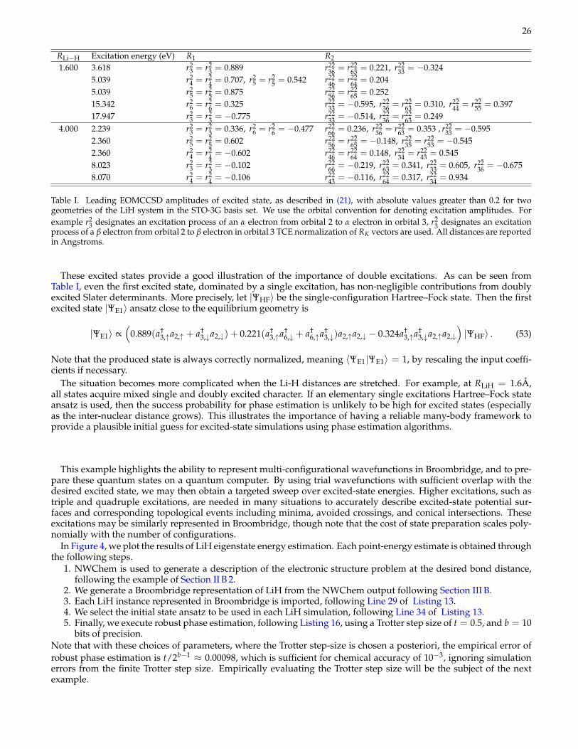
26

RLi−H Excitation energy (eV) R1 R2

1.600 3.618 r23 = r2

3 = 0.889 r2236 = r22

63 = 0.221, r2233 = −0.324

5.039 r24 = r2

4 = 0.707, r25 = r2

5 = 0.542 r2246 = r22

64 = 0.2045.039 r2

5 = r25 = 0.875 r22

56 = r2265 = 0.252

15.342 r26 = r2

6 = 0.325 r2233 = −0.595, r22

36 = r2263 = 0.310, r22

44 = r2255 = 0.397

17.947 r23 = r2

3 = −0.775 r2233 = −0.514, r22

36 = r2263 = 0.249

4.000 2.239 r23 = r2

3 = 0.336, r26 = r2

6 = −0.477 r2266 = 0.236, r22

36 = r2263 = 0.353 , r22

33 = −0.5952.360 r2

5 = r25 = 0.602 r22

56 = r2265 = −0.148, r22

35 = r2253 = −0.545

2.360 r24 = r2

4 = −0.602 r2246 = r22

64 = 0.148, r2234 = r22

43 = 0.5458.023 r2

3 = r23 = −0.102 r22

66 = −0.219, r2263 = 0.341, r22

33 = 0.605, r2236 = −0.675

8.070 r24 = r2

4 = −0.106 r2243 = −0.116, r22

64 = 0.317, r2234 = 0.934

Table I. Leading EOMCCSD amplitudes of excited state, as described in (21), with absolute values greater than 0.2 for twogeometries of the LiH system in the STO-3G basis set. We use the orbital convention for denoting excitation amplitudes. Forexample r2

3 designates an excitation process of an α electron from orbital 2 to α electron in orbital 3, r23 designates an excitation

process of a β electron from orbital 2 to β electron in orbital 3 TCE normalization of RK vectors are used. All distances are reportedin Angstroms.

These excited states provide a good illustration of the importance of double excitations. As can be seen fromTable I, even the first excited state, dominated by a single excitation, has non-negligible contributions from doublyexcited Slater determinants. More precisely, let |ΨHF〉 be the single-configuration Hartree–Fock state. Then the firstexcited state |ΨE1〉 ansatz close to the equilibrium geometry is

|ΨE1〉 ∝(

0.889(a†3,↑a2,↑ + a†

3,↓a2,↓) + 0.221(a†3,↑a

†6,↓ + a†

6,↑a†3,↓)a2,↑a2,↓ − 0.324a†

3,↑a†3,↓a2,↑a2,↓

)|ΨHF〉 . (53)

Note that the produced state is always correctly normalized, meaning 〈ΨE1|ΨE1〉 = 1, by rescaling the input coeffi-cients if necessary.

The situation becomes more complicated when the Li-H distances are stretched. For example, at RLiH = 1.6Å,all states acquire mixed single and doubly excited character. If an elementary single excitations Hartree–Fock stateansatz is used, then the success probability for phase estimation is unlikely to be high for excited states (especiallyas the inter-nuclear distance grows). This illustrates the importance of having a reliable many-body framework toprovide a plausible initial guess for excited-state simulations using phase estimation algorithms.

This example highlights the ability to represent multi-configurational wavefunctions in Broombridge, and to pre-pare these quantum states on a quantum computer. By using trial wavefunctions with sufficient overlap with thedesired excited state, we may then obtain a targeted sweep over excited-state energies. Higher excitations, such astriple and quadruple excitations, are needed in many situations to accurately describe excited-state potential sur-faces and corresponding topological events including minima, avoided crossings, and conical intersections. Theseexcitations may be similarly represented in Broombridge, though note that the cost of state preparation scales poly-nomially with the number of configurations.

In Figure 4, we plot the results of LiH eigenstate energy estimation. Each point-energy estimate is obtained throughthe following steps.

1. NWChem is used to generate a description of the electronic structure problem at the desired bond distance,following the example of Section II B 2.

2. We generate a Broombridge representation of LiH from the NWChem output following Section III B.3. Each LiH instance represented in Broombridge is imported, following Line 29 of Listing 13.4. We select the initial state ansatz to be used in each LiH simulation, following Line 34 of Listing 13.5. Finally, we execute robust phase estimation, following Listing 16, using a Trotter step size of t = 0.5, and b = 10

bits of precision.Note that with these choices of parameters, where the Trotter step-size is chosen a posteriori, the empirical error ofrobust phase estimation is t/2b−1 ≈ 0.00098, which is sufficient for chemical accuracy of 10−3, ignoring simulationerrors from the finite Trotter step size. Empirically evaluating the Trotter step size will be the subject of the nextexample.

27

1 2 3 4 5-8.0

-7.8

-7.6

-7.4

-7.2

-7.0

RLi-H / Angstrom

Energy/Hartree

Ground and excited energy sweeps using EOMCCSD wavefunction ansatz

Figure 4. Estimated eigenstate energies as a function of RLi-H bonding distance obtained using robust phase estimation witha Trotter step size of t = 0.5, b = 10 bits of precision, and two repetitions at each bonding distance per energy level. Errorbars correspond to contribution of the phase estimation procedure alone, and are exaggerated by a factor of 5 for clarity. ExactFCI energies are plotted (gray) for comparison. Different colored points correspond to initial state ansatzes targeted at differentenergy levels. Each ansatz is multi-configurational with up to the first 12 dominant coefficients included. This enables a selectivesweep of the desired excited-state energy, though observe that at large bond distances, particularly the fourth excited state, theansatz may still have a low probability of projecting onto the exact eigenstate.

B. Empirical Trotter error estimation of stretched H10 chains

The H10 system epitomizes many of the correlation effects encountered in realistic strongly correlated molecularsystems. This system has been recently used in studies of various methods designed to deal with strong quasi-degeneracy effects [67] as the degree of multi-configurational character of the ground-state wavefunction can bevaried by changing the hydrogen-hydrogen distance R in a linear chain of the hydrogen atoms. For example, atR = 1.0 a.u., the corresponding wavefunction is dominated by a single restricted Hartree–Fock determinant. How-ever stretching the R distance to 3.6 a.u. results in a multi-reference character of the wavefunction, which posesa significant challenge for single reference CC methods using RHF reference. Among several methods tested inRef. [66], the auxiliary-field quantum Monte Carlo (AFQMC), density matrix embedding theory (DMET), UHF-CC, and self-energy embedding theory (SEET) formalisms lent themselves to coping with strong correlation effects.Other formalisms such as self-consistent second-order Green’s function (GF2) and RHF-CC approximations suffersignificant deterioration in energy accuracies especially for stretched geometries. For this reason, the H10 system isan ideal target for testing various elements of quantum algorithms for electronic structure problems. We also com-pare and discuss the accuracies of state-selective multi-reference coupled-cluster (MRCC) methods, represented hereby the Mukherjee’s MRCC approach (MkMRCC) [68, 69], which was not studied in Ref. [66].

We perform quantum simulations within an STO-6G minimal basis consisting of 20 spin orbitals. The results ofrobust phase estimation on a first-order Trotter-Suzuki formula, similar to LiH in the previous section, are comparedto various classical approaches. The MkMRCC formalism has been tested using its two variants: MkMRCC modelwith singles and doubles (MkMRCCSD) and MkMRCCSD with perturbative triples corrections (MkMRCCSD(T));see [70–72]. In Table II, we have also collated CCSDT [73–75] and CCSDTQ [76, 77] ground-state energies, whichalso have not been studied in Ref. [66].

As a result of strong quasi-degeneracy effects, both CCSD and CCSDT energies start to significantly deviate fromtheir FCI counterparts for stretched geometries. Although the non-variational collapse of the CCSDT energies isnot as profound as in the CCSD case, we notice a sizable CCSDT energy error of 47 milliHartree at R = 3.6 a.u.The addition of quadruple excitations in the CCSDTQ method offsets the variational collapse of the CCSD method.However, a 4 milliHartree still persists for larger distances.

Although resorting to the MkMRCCSD formalism significantly improves the quality of energies in the R = 1.0 a.u.

28

R (a.u.) FCI (Hartree) Difference from FCI (10−3 Hartree)CCSD CCSDT CCSDTQ MkMRCCSD MkMRCCSD(T) RPE

1.0 -3.82439 0.5 0.0 0.0 0.1 -0.1 -1.9 ± 0.81.2 -4.76638 0.8 0.0 0.0 0.0 -0.2 -0.7 ± 0.61.4 -5.20509 1.1 -0.1 0.0 0.0 -0.5 -0.3 ± 0.51.6 -5.38436 1.4 -0.2 0.0 -0.1 -0.8 0.0 ± 0.51.8 -5.42439 1.8 -0.5 0.0 -0.3 -1.4 1.5 ± 1.22.0 -5.38963 2.2 -1.1 0.0 -0.4 -2.2 -1.7 ± 0.82.4 -5.22794 1.1 -5.6 0.0 0.3 -4.0 -0.7 ± 0.82.8 -5.05024 -17.1 -32.7 0.6 0.6 -8.9 -0.8 ± 0.53.2 -4.91038 -990.0 -888.0 3.5 -1.3 -19.4 -0.4 ± 0.43.6 -4.81870 -111.0 -47.3 4.5 -43.3 ± 1.0 -74.3 ± 1.0 0.7 ± 1.1

Table II. Comparison of energies with respect to bond distance R obtained by phase estimation through the Microsoft QuantumDevelopment Kit Robust Phase Estimation (RPE) algorithm with energies obtained by various CC methodologies for the H10system in the STO-6G basis set. In all CC calculations, restricted Hartree–Fock molecular orbitals are used.

to R = 3.2 a.u. region, the MkMRCCSD approach still yields large negative errors at R = 3.6 a.u.. This situation ismostly a consequence of an inadequate choice of model space and the resulting intruder state problem [78]. Theseare manifestations of divergent perturbation theory expansions that occur in near-degenerate systems and are theculprits behind the divergent character of MkMRCCSD(T) correction.

Phase estimation approaches on quantum computers remove the biases introduced by the use of reference func-tion, model space, and level of excitation. In contrast to other results collated in Table II, phase estimation produceserrors of small uniform size for all geometries. This is especially important for stretched geometries, particularlyR = 3.6 a.u., where the CCSD, CCSDT, MkMRCCSD, and MkMRCCSD(T) approaches reveal singular behavior.Even though the failure of the CCSDTQ approach is not as pronounced as it is in the other cases, the CCSDTQ en-ergy error of 4.5 milliHartree for R = 3.6 a.u. is significantly larger than the 0.7 milliHartree error obtained withphase estimation. In principle, the error of phase estimation can be made arbitrarily small, at a modest propor-tionately higher cost. This presents a strong argument in favor of using quantum simulation algorithms withinquasi-degenerate or metallic regimes.

In these examples, the Trotter number chosen for the Trotter–Suzuki formula, which is the inverse of the Trotterstep-size as described after (30), in the phase estimation algorithm can be found in Figure 5. We see that, despite theerrors in all the coupled-cluster methods considered in Table II that increasing with R, the Trotter number needed toachieve chemical accuracy actually decreases monotonically with R, which corresponds to a more efficient quantumsimulation. This increase is unsurprising as the Coulomb interaction between electrons, which typically dominateserrors in the quantum simulation algorithms, weaken when the molecule stretches.

A major strength arising from the integration of Q# and NWChem is the ability to automate these sweeps of theFCI energy as a function of R. This automation means that studies of phase estimation over different spacings in H10,or surveys of hydrogen chains of different lengths, can be easily generated inside a single framework. Furthermore,all code written for these simulations will still be useful once quantum computers are built that can reliably performphase estimation on H10 because of the simulator model used within Q# forbids the language from distinguishingbetween the simulator and a quantum computer. This work provides a preview of the types of studies that auto-mated quantum computer simulations of chemistry will one day enable while illustrating the challenges that can befaced by classical methods for even simple molecules.

In Figure 5, we plot the results of H10 eigenstate energy estimation. Each point-energy estimate is obtained asfollows.

1. NWChem is used to generate a description of the electronic structure problem at the desired bond distance,following Section II B 2.

2. We generate a Broombridge representation of H10 from the NWChem output following Section III B.3. Each H10 instance represented in Broombridge is imported, following Line 29 of Listing 13.4. Select the ground-state ansatz in Broombridge, following Line 34 of Listing 13.5. Execute robust phase estimation, following Listing 16, using a Trotter step size t ∈ [tmin, tmax] uniformly sam-

pled on a log scale, and some b bits of precision.In contrast to Section V A, where the Trotter number r = 1/t and bits of precision b were chosen a posteriori, weempirically determine the Trotter step-size t required to control the error contribution ∆ from the Trotter–Suzuki

29

-5.3913(8)

R= 2.0 a.u.

-0.2 0.0 0.2 0.4 0.6 0.8

+0.

+0.05

+0.1

+0.15

Log10(Trotter number)

Energy/Hartree

-3.8263(8)

R= 1.0 a.u.

+0.

+0.05

+0.1

+0.15

Energy/Hartree

-5.2286(8)

R= 2.4 a.u.

-0.2 0.0 0.2 0.4 0.6 0.8Log10(Trotter number)

-4.7671(6)

R= 1.2 a.u.

-5.0510(5)

R= 2.8 a.u.

-0.2 0.0 0.2 0.4 0.6 0.8Log10(Trotter number)

-5.2054(5)

R= 1.4 a.u.

-4.9104(3)

R= 3.2 a.u.

-0.2 0.0 0.2 0.4 0.6 0.8Log10(Trotter number)

-5.3844(5)

R= 1.6 a.u.

-4.8180(11)

R= 3.6 a.u.

-0.2 0.0 0.2 0.4 0.6 0.8

+0.

+0.05

+0.1

+0.15

Log10(Trotter number)

-5.4229(12)

R= 1.8 a.u.

+0.

+0.05

+0.1

+0.15

Figure 5. Estimated ground-state energy E (orange) as a function of Trotter number r of the first-order integrator ∏j e−iHj/r forH10 at various bond distances obtained by a least-squares fit to E = m

r2 + E0 (blue), where m, E0 are fit parameters. The ground-state energy estimate E0, which is assumed to be normal distributed, is also plotted (yellow) with its standard deviation providedin round brackets. Error bars represent the standard deviation of E0 by robust phase estimation, given the prior that E0 lies in theplotted range. Dotted error bars (gray) are excluded from the fit as they either have a large Trotter–Suzuki error, or correspond toexcited states. The shaded region (green) corresponds to a Trotter number that achieves at least chemical accuracy based on thefit m

r2 ≤ 0.001 Hartree.

integrator. We do so by applying the known error scaling from (30)∥∥∥∥∥e−iHt −M

∏j=1

e−ihjPjt

∥∥∥∥∥ = O(t2) (54)

for the first-order integrator that is used here. Thus, in the limit of sufficient small t, the estimated ground stateenergy E ought to scale as

E = E0 + ∆ = E0 + mt2 +O(t3), (55)

where E0 is the exact ground-state energy and m is a constant. Thus, performing phase estimation on E for variousstep sizes t allows us to obtain data that we fit to obtain E0 and m, in the regime where the quadratic t2 scaling is ob-served to be dominant. Note that by repeating O(1/∆2) times, achieving chemical accuracy is possible through thefit, even if the sampling error from a single run of phase estimation is large. However, overall quantum gate complex-ity is always minimized by performing a logarithmic number of high-precision estimates which takes O(1/∆) time,rather than the O(1/∆2) time required by naïve sampling. In particular, the fitted energy estimates can be highlyaccurate even if all individual data points have both a Trotter–Suzuki approximation error and a phase estimationerror larger than chemical accuracy.

C. Quantum computing predictions and resource estimations for C20 isomerizations

The relative energies of the three C20 fullerene, bowl, and ring isomers have been a subject of intensive theo-retical studies spanning nearly three decades [79–92]. Although these three isomers have been widely examined

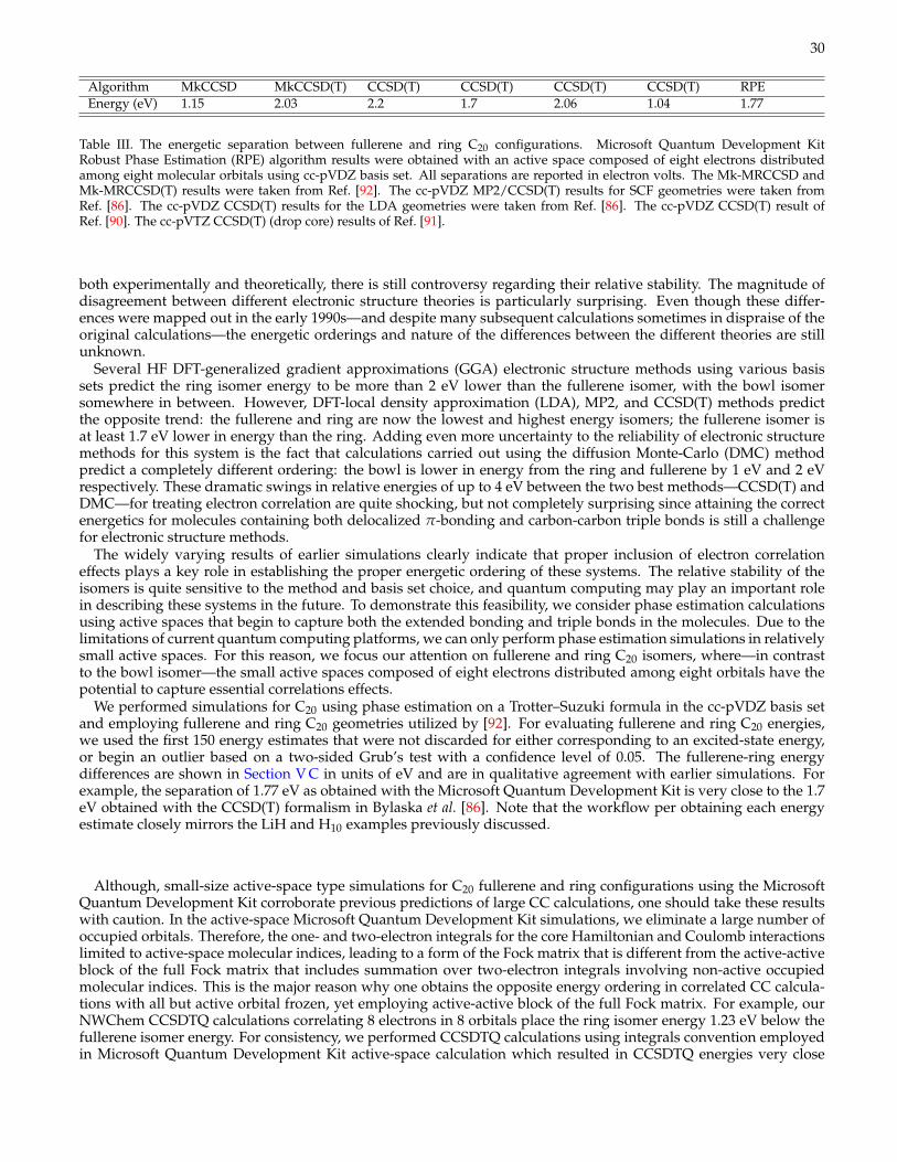
30

Algorithm MkCCSD MkCCSD(T) CCSD(T) CCSD(T) CCSD(T) CCSD(T) RPEEnergy (eV) 1.15 2.03 2.2 1.7 2.06 1.04 1.77

Table III. The energetic separation between fullerene and ring C20 configurations. Microsoft Quantum Development KitRobust Phase Estimation (RPE) algorithm results were obtained with an active space composed of eight electrons distributedamong eight molecular orbitals using cc-pVDZ basis set. All separations are reported in electron volts. The Mk-MRCCSD andMk-MRCCSD(T) results were taken from Ref. [92]. The cc-pVDZ MP2/CCSD(T) results for SCF geometries were taken fromRef. [86]. The cc-pVDZ CCSD(T) results for the LDA geometries were taken from Ref. [86]. The cc-pVDZ CCSD(T) result ofRef. [90]. The cc-pVTZ CCSD(T) (drop core) results of Ref. [91].

both experimentally and theoretically, there is still controversy regarding their relative stability. The magnitude ofdisagreement between different electronic structure theories is particularly surprising. Even though these differ-ences were mapped out in the early 1990s—and despite many subsequent calculations sometimes in dispraise of theoriginal calculations—the energetic orderings and nature of the differences between the different theories are stillunknown.

Several HF DFT-generalized gradient approximations (GGA) electronic structure methods using various basissets predict the ring isomer energy to be more than 2 eV lower than the fullerene isomer, with the bowl isomersomewhere in between. However, DFT-local density approximation (LDA), MP2, and CCSD(T) methods predictthe opposite trend: the fullerene and ring are now the lowest and highest energy isomers; the fullerene isomer isat least 1.7 eV lower in energy than the ring. Adding even more uncertainty to the reliability of electronic structuremethods for this system is the fact that calculations carried out using the diffusion Monte-Carlo (DMC) methodpredict a completely different ordering: the bowl is lower in energy from the ring and fullerene by 1 eV and 2 eVrespectively. These dramatic swings in relative energies of up to 4 eV between the two best methods—CCSD(T) andDMC—for treating electron correlation are quite shocking, but not completely surprising since attaining the correctenergetics for molecules containing both delocalized π-bonding and carbon-carbon triple bonds is still a challengefor electronic structure methods.

The widely varying results of earlier simulations clearly indicate that proper inclusion of electron correlationeffects plays a key role in establishing the proper energetic ordering of these systems. The relative stability of theisomers is quite sensitive to the method and basis set choice, and quantum computing may play an important rolein describing these systems in the future. To demonstrate this feasibility, we consider phase estimation calculationsusing active spaces that begin to capture both the extended bonding and triple bonds in the molecules. Due to thelimitations of current quantum computing platforms, we can only perform phase estimation simulations in relativelysmall active spaces. For this reason, we focus our attention on fullerene and ring C20 isomers, where—in contrastto the bowl isomer—the small active spaces composed of eight electrons distributed among eight orbitals have thepotential to capture essential correlations effects.

We performed simulations for C20 using phase estimation on a Trotter–Suzuki formula in the cc-pVDZ basis setand employing fullerene and ring C20 geometries utilized by [92]. For evaluating fullerene and ring C20 energies,we used the first 150 energy estimates that were not discarded for either corresponding to an excited-state energy,or begin an outlier based on a two-sided Grub’s test with a confidence level of 0.05. The fullerene-ring energydifferences are shown in Section V C in units of eV and are in qualitative agreement with earlier simulations. Forexample, the separation of 1.77 eV as obtained with the Microsoft Quantum Development Kit is very close to the 1.7eV obtained with the CCSD(T) formalism in Bylaska et al. [86]. Note that the workflow per obtaining each energyestimate closely mirrors the LiH and H10 examples previously discussed.

Although, small-size active-space type simulations for C20 fullerene and ring configurations using the MicrosoftQuantum Development Kit corroborate previous predictions of large CC calculations, one should take these resultswith caution. In the active-space Microsoft Quantum Development Kit simulations, we eliminate a large number ofoccupied orbitals. Therefore, the one- and two-electron integrals for the core Hamiltonian and Coulomb interactionslimited to active-space molecular indices, leading to a form of the Fock matrix that is different from the active-activeblock of the full Fock matrix that includes summation over two-electron integrals involving non-active occupiedmolecular indices. This is the major reason why one obtains the opposite energy ordering in correlated CC calcula-tions with all but active orbital frozen, yet employing active-active block of the full Fock matrix. For example, ourNWChem CCSDTQ calculations correlating 8 electrons in 8 orbitals place the ring isomer energy 1.23 eV below thefullerene isomer energy. For consistency, we performed CCSDTQ calculations using integrals convention employedin Microsoft Quantum Development Kit active-space calculation which resulted in CCSDTQ energies very close

31

Generic Qubitization Optimized QubitizationGeometry N η Qubits T gates Rz L1 norm Qubits T gates Rz L1 norm (56) × T gatesRing 50 32 143 9278072 17931406 1539 312 18605634 18 962 1.8× 1013

Fullerene 50 32 145 18514478 3586938 2004 316 37078492 18 1392 5.2× 1013

Bowl 50 32 145 26153750 36815676 2297 316 52357100 18 1480 7.7× 1013

Ring 17 14 63 121574 145222 315 210 252860 18 294 7.4× 1010

Fullerene 17 14 65 242664 292166 448 214 495158 18 418 2.1× 1011

Bowl 17 14 67 357458 569110 411 218 724880 18 384 2.8× 1011

Table IV. Resources required to perform a single quantum walk step created by the Qubitization procedure for different config-urations of C20 in the cc-pVDZ basis set, with η electrons and varying numbers of N orbitals within the active space. Here allHamiltonian terms below with norm below 10−10 Hartree are truncated and the L1 norm is the sum of the absolute values ofthe Hamiltonian terms in Jordan–Wigner representation. Generic qubitization refers to the unoptimized procedure as describedin Section II C 3, whereas optimized Qubitization applies chemistry-specific optimizations described in Section II C 4. The ex-pected number of T gates needed to synthesize nRz rotations within total error at most ε (without the use of ancillæ) is boundedabove by 3nRz (log2 (nRz /ε) +O(log log (nRz /ε))) [54], where ∆ = 1 milliHartree for chemical accuracy. The rightmost rowstates the total number of T gates required for an energy estimate of the ground state to chemical accuracy.

to ones obtained in Microsoft Quantum Development Kit simulations. This disagreement may be resolved eitherthrough Microsoft Quantum Development Kit simulations employing particle-hole representation of creation/anni-hilation operators [93] or by employing larger active spaces, as discussed next.

1. Resource estimation for simulating C20 isomers

Until fault-tolerant quantum computers are available, classical simulations of quantum chemistry at chemical ac-curacy are limited to 40− 50 spin orbitals. Nevertheless, we may still obtain estimates of the quantum resourcesrequired to execute these classically intractable examples. Resource estimates are tabulated in Table IV for two im-plementations of qubitization: one unoptimized and the other optimized for chemistry as described in Section II C 4.Data in each row are obtained by the following procedure:

1. NWChem is used to generate a description of the electronic structure problem in the desired configuration,following Section II B 2.

2. We generate a Broombridge representation of C20 from the NWChem output following Section III B.3. The C20 instance represented in Broombridge is imported, following Line 29 of Listing 13.4. Qubitization is chosen as the simulation method, both with and without optimization, following Line 24 of

Listing 15.5. A single step of the qubitization walk operator is run through the Trace simulator, which yields resource esti-

mates needed for the simulation, following Listing 3.The output of the Trace simulator is tabulated in Table IV. We see from the data included that the costs of im-

plementing the qubitization walk operator is substantially reduced through the use of the optimizations discussedin Line 24. In particular, for the case where C20 is configured in a ring with an active space consisting of 50 orbitalsand using 1 milliHartree as our target precision, we find that if an ancilla-free synthesis method is used then theexpected total number of T gates needed to perform the walk operator is roughly 1.8× 109. The majority of thiscost arises from synthesis of arbitrary single-qubit rotations with a fault-tolerant gate set. If we use the optimizedapproach, then the number of gates required is reduced by nearly a factor of 100 to 1.8× 107 T gates. The remain-ing cases see similar improvements, underlining the importance of problem-specific optimization of the subroutinesused in qubitization.

As a final example, let us consider the problem of computing the number of gates that would be needed to estimatethe ground-state energy within error ε using qubitization. From (48), the number of applications of a unitary requiredto obtain a phase estimate with standard deviation ∆ Hartree is ≈ 1/∆. Combined with the phase-doubling trickof [26], the number of applications of the qubitization walk operator is approximately

Lexp ≈L1 norm

2∆. (56)

As the spectrum of the quantum walk is exactly similar to arcsin[H/h] ≈ H/h, the only other error contribution isfrom the finite precision of Hamiltonian coefficients realized in the quantum circuit. However, we may ignore thiserror contribution as it can be made arbitrarily small without changing the T-count, to leading order in the optimizedqubitization scheme.

32

By using this formula, we obtain estimates T gate count for sampling from the Hamiltonian spectrum to chemicalaccuracy. We find that the number of T gates needed for the simulation (for the ring geometry) is expected to beless than 1.8× 1013. The number of spin orbitals required in this case are 100, which places the scale on the sameorder of magnitude as that estimated for Trotter-based simulations for FeMoco given in [5]. Similarly, we findthat the number of T gates is within an order of magnitude of the 1014 gates required for a qualitatively accuratesimulation for the 108 spin-orbital example of FeMoco considered therein. A crucial difference however is that theFeMoco gate estimates required a certain optimistic extrapolation of empirical Trotter step-size from small, classicallysimulable molecules. In contrast, the qubitization T gate estimate is fully rigorous, assuming the ground truth of thepresented Hamiltonian. This further suggests that optimized variants qubitization may be preferable to Trotter–Suzuki simulations for challenging problems in general.

VI. CONCLUSIONS

Today, the steady progress of scalable fault-tolerant quantum computing from theory to reality drives intenseresearch in its use. Many promising quantum algorithms are already known and more continue to be developedat a furious pace. Paralleling the history of classical computing, we may expect that algorithmic advances willcontribute far more to the overall computational capability of quantum computers than optimistic Moore’s-Lawhardware scaling predictions. However, the many envisioned applications of quantum computing, particularly thatof electronic structure problems, are highly inter-disciplinary. The current barrier to their use by non-specialists inquantum computing—the intended audience—is, more often than not, insurmountable. In many cases, effective useof these algorithms requires knowledge of low-level details such as error-correction schemes and specialized circuitoptimizations.

When the requisite quantum hardware arrives, its use should be accessible, reproducible, and extensible. Theopen-source tools and workflow we present here are intended to realize this vision. Accessibility by the targetaudience is achieved by using NWChem, a standard classical computational chemistry packages, as the access point,followed by the integration with quantum algorithms that are expressed and invoked at a high-level in our chemistrylibrary. Reproducibility through our proposed workflow allows for a straightforward and consistent application tofuture problems of scientific and industrial interest. Extensibility of our work to future algorithmic improvementson both the classical and quantum side remains possible through our definition of standardized interfaces, such asBroombridge, for representing electronic structure problems.

The examples we provide and their results underscore the value of the workflow enabled by integrating Q# withNWChem. By combining the two, we are capable of generating end-to-end resource estimates for simulation thatare not only accurate but are also highly optimized and reproducible. This illustrates that by building libraries tocompute accurate electronic structure representations and also by building highly optimized libraries for quantumsimulation targeted at quantum hardware, we can create tools that empower people to explore and cost quantumchemistry simulation algorithms without requiring that the user be an expert in both fields.

This work highlights the impact that scientific software development can have on reproducible research. It isour hope that this work helps chemists, physicists, and computer scientists to pool their knowledge so as to enablequantum methods for electronic structure calculation to reach the same level of sophistication and value as classicalcomputing today already achieves. More broadly, we hope to inspire the development of new libraries, platforms,and even programming languages that facilitate the entry of new researchers into the interdisciplinary field of quan-tum computing and eventually be constructively used to solve the intractable quantum problems of today.

ACKNOWLEDGMENTS

We thank the broader Microsoft Quantum team for insightful comments and discussions. The PNNL portion ofthis research was funded by the Quantum Algorithms, Software, and Architectures (QUASAR) Initiative, conductedunder the Laboratory Directed Research and Development Program at PNNL. KK and EJB also acknowledge supportfrom the ‘Embedding Quantum Computing into Many-body Frameworks for Strongly Correlated Molecular andMaterials Systems’ project, which is funded by the U.S. Department of Energy (DOE), Office of Science, Office of BasicEnergy Sciences, the Division of Chemical Sciences, Geosciences, and Biosciences. The development of NWChemwas supported from Environmental Molecular Sciences Laboratory (EMSL) operations. Environmental MolecularSciences Laboratory (EMSL) operations are supported by the DOE Office of Biological and Environmental Research.The Pacific Northwest National Laboratory, is operated for the U.S. DOE by Battelle under Contract Number DE-

33

AC05-76RL01830.

[1] W. Koch and M. C. Holthausen, Journal of the American Chemical Society (Wiley-VCH Verlag GmbH, Weinheim, FRG, 2001).[2] R. J. Bartlett and M. Musiał, “Coupled-cluster theory in quantum chemistry,” Reviews of Modern Physics 79, 291 (2007).[3] U. Schollwöck, “The density-matrix renormalization group,” Reviews of Modern Physics 77, 259 (2005).[4] M. A. Nielsen and I. L. Chuang, Quantum Computation and Quantum Information, 1st ed. (Cambridge University Press, 2004).[5] M. Reiher, N. Wiebe, K. M. Svore, D. Wecker, and M. Troyer, “Elucidating reaction mechanisms on quantum computers,”

Proceedings of the National Academy of Sciences 114, 7555 (2017), arXiv:1605.03590.[6] D. Wecker, M. B. Hastings, N. Wiebe, B. K. Clark, C. Nayak, and M. Troyer, “Solving strongly correlated electron models on

a quantum computer,” Physical Review A 92, 062318 (2015).[7] B. Bauer, D. Wecker, A. J. Millis, M. B. Hastings, and M. Troyer, “Hybrid Quantum-Classical Approach to Correlated Mate-

rials,” Physical Review X 6, 031045 (2016).[8] S. Lloyd, “Universal Quantum Simulators,” Science 273, 1073 (1996).[9] D. Aharonov and A. Ta-Shma, “Adiabatic quantum state generation and statistical zero knowledge,” in Proceedings of the

thirty-fifth ACM symposium on Theory of computing - STOC ’03, STOC ’03 (ACM Press, New York, New York, USA, 2003) p. 20.[10] D. W. Berry, G. Ahokas, R. Cleve, and B. C. Sanders, “Efficient Quantum Algorithms for Simulating Sparse Hamiltonians,”

Communications in Mathematical Physics 270, 359 (2007).[11] D. W. Berry and A. M. Childs, “Black-box Hamiltonian simulation and unitary implementation,” Quantum Information &

Computation 12, 29 (2012), arXiv:0910.4157.[12] D. W. Berry, A. M. Childs, R. Cleve, R. Kothari, and R. D. Somma, “Simulating Hamiltonian Dynamics with a Truncated

Taylor Series,” Physical Review Letters 114, 090502 (2015).[13] G. H. Low and I. L. Chuang, “Optimal Hamiltonian Simulation by Quantum Signal Processing,” Physical Review Letters

118, 010501 (2017), arXiv:1606.02685.[14] G. H. Low and I. L. Chuang, “Hamiltonian Simulation by Qubitization,” arXiv preprint arXiv:1610.06546 (2016),

arXiv:1610.06546.[15] J. Haah, M. Hastings, R. Kothari, and G. H. Low, “Quantum Algorithm for Simulating Real Time Evolution of Lattice

Hamiltonians,” in 2018 IEEE 59th Annual Symposium on Foundations of Computer Science (FOCS), FOCS ’18 (IEEE, Washington,DC, USA, 2018) pp. 350–360.

[16] G. H. Low and N. Wiebe, “Hamiltonian Simulation in the Interaction Picture,” arXiv preprint arXiv:1805.00675 (2018),arXiv:1805.00675.

[17] E. Campbell, “A random compiler for fast Hamiltonian simulation,” arXiv preprint arXiv:1811.08017 (2018),arXiv:1811.08017.

[18] D. S. Abrams and S. Lloyd, “Simulation of Many-Body Fermi Systems on a Universal Quantum Computer,” Physical ReviewLetters 79, 2586 (1997).

[19] J. D. Whitfield, J. Biamonte, and A. Aspuru-Guzik, “Simulation of electronic structure Hamiltonians using quantum com-puters,” Molecular Physics 109, 735 (2011).

[20] R. Babbush, D. W. Berry, I. D. Kivlichan, A. Y. Wei, P. J. Love, and A. Aspuru-Guzik, “Exponentially more precise quantumsimulation of fermions in second quantization,” New Journal of Physics 18, 033032 (2016).

[21] D. Wecker, B. Bauer, B. K. Clark, M. B. Hastings, and M. Troyer, “Gate-count estimates for performing quantum chemistryon small quantum computers,” Physical Review A 90, 022305 (2014).

[22] D. Poulin, M. B. Hastings, D. Wecker, N. Wiebe, A. C. Doberty, M. Troyer, A. C. Doherty, and M. Troyer, “The Trotter stepsize required for accurate quantum simulation of quantum chemistry,” Quantum Information & Computation 15, 361 (2015),arXiv:1406.4920.

[23] M. B. Hastings, D. Wecker, B. Bauer, and M. Troyer, “Improving Quantum Algorithms for Quantum Chemistry,” QuantumInformation & Computation 15, 1 (2015).

[24] R. Babbush, J. McClean, D. Wecker, A. Aspuru-Guzik, and N. Wiebe, “Chemical basis of Trotter-Suzuki errors in quantumchemistry simulation,” Physical Review A 91, 022311 (2015).

[25] A. M. Childs, D. Maslov, Y. Nam, N. J. Ross, and Y. Su, “Toward the first quantum simulation with quantum speedup,”Proceedings of the National Academy of Sciences 115, 9456 (2018).

[26] R. Babbush, C. Gidney, D. W. Berry, N. Wiebe, J. McClean, A. Paler, A. Fowler, and H. Neven, “Encoding Electronic Spectrain Quantum Circuits with Linear T Complexity,” arXiv (2018).

[27] J. R. McClean, J. Romero, R. Babbush, and A. Aspuru-Guzik, “The theory of variational hybrid quantum-classical algo-rithms,” New Journal of Physics 18, 023023 (2016).

[28] N. C. Rubin, R. Babbush, and J. McClean, “Application of fermionic marginal constraints to hybrid quantum algorithms,”New Journal of Physics 20, 053020 (2018).

[29] Y. Cao, J. Romero, J. P. Olson, M. Degroote, P. D. Johnson, M. Kieferová, I. D. Kivlichan, T. Menke, B. Peropadre, N. P. D.Sawaya, S. Sim, L. Veis, and A. Aspuru-Guzik, “Quantum Chemistry in the Age of Quantum Computing,” arXiv preprintarXiv:1812.09976 (2018), arXiv:1812.09976.

[30] A. S. Green, P. L. Lumsdaine, N. J. Ross, P. Selinger, and B. Valiron, “Quipper,” in ACM SIGPLAN Notices, Vol. 48 (ACM,2013) p. 333.

34

[31] D. Wecker and K. M. Svore, “LIQUi|〉: A Software Design Architecture and Domain-Specific Language for Quantum Com-puting,” arXiv preprint arXiv:1402.4467 (2014), arXiv:1402.4467.

[32] D. S. Steiger, T. Häner, and M. Troyer, “ProjectQ: an open source software framework for quantum computing,” Quantum 2,49 (2018).

[33] A. W. Cross, L. S. Bishop, J. A. Smolin, and J. M. Gambetta, “Open Quantum Assembly Language,” arXiv preprintarXiv:1707.03429 (2017), arXiv:1707.03429.

[34] K. Svore, A. Geller, M. Troyer, J. Azariah, C. Granade, B. Heim, V. Kliuchnikov, M. Mykhailova, A. Paz, and M. Roetteler,“Q#: Enabling scalable quantum computing and development with a high-level domain-specific language,” in Proceedingsof the Real World Domain Specific Languages Workshop 2018 on - RWDSL2018, RWDSL2018 (ACM Press, New York, New York,USA, 2018) pp. 1–10.

[35] J. R. McClean, T. Häner, D. S. Steiger, and R. Babbush, FermiLib v0. 1, Tech. Rep. (Lawrence Berkeley National Lab.(LBNL),Berkeley, CA (United States), 2017).

[36] J. R. McClean, K. J. Sung, I. D. Kivlichan, Y. Cao, C. Dai, E. S. Fried, C. Gidney, B. Gimby, P. Gokhale, T. Häner, T. Hardikar,V. Havlícek, O. Higgott, C. Huang, J. Izaac, Z. Jiang, X. Liu, S. McArdle, M. Neeley, T. O’Brien, B. O’Gorman, I. Ozfidan,M. D. Radin, J. Romero, N. Rubin, N. P. D. Sawaya, K. Setia, S. Sim, D. S. Steiger, M. Steudtner, Q. Sun, W. Sun, D. Wang,F. Zhang, and R. Babbush, “OpenFermion: The Electronic Structure Package for Quantum Computers,” arXiv preprintarXiv:1710.07629 (2017), arXiv:1710.07629.

[37] J. Preskill, “Quantum Computing in the NISQ era and beyond,” Quantum 2, 79 (2018).[38] A. Kandala, A. Mezzacapo, K. Temme, M. Takita, M. Brink, J. M. Chow, and J. M. Gambetta, “Hardware-efficient variational

quantum eigensolver for small molecules and quantum magnets,” Nature 549, 242 (2017).[39] M. Valiev, E. Bylaska, N. Govind, K. Kowalski, T. Straatsma, H. Van Dam, D. Wang, J. Nieplocha, E. Apra, T. Windus,

and W. de Jong, “NWChem: A comprehensive and scalable open-source solution for large scale molecular simulations,”Computer Physics Communications 181, 1477 (2010).

[40] M. M. Waldrop, “The chips are down for Moore’s law,” Nature 530, 144 (2016).[41] G. Meszaros, xUnit test patterns: Refactoring test code (Pearson Education, 2007).[42] D. E. Bernholdt, E. E. Aprà, H. A. Früchtl, M. F. Guest, R. J. Harrison, R. A. Kendall, R. A. Kutteh, X. Long, J. B. Nicholas,

J. A. Nichols, H. L. Taylor, A. T. Wong, G. I. Fann, R. J. Littlefield, and J. Nieplocha, “Parallel computational chemistry madeeasier: The development of NWChem,” International Journal of Quantum Chemistry 56, 475 (1995).

[43] R. A. Kendall, E. Aprà, D. E. Bernholdt, E. J. Bylaska, M. Dupuis, G. I. Fann, R. J. Harrison, J. Ju, J. A. Nichols, J. Nieplocha,T. Straatsma, T. L. Windus, and A. T. Wong, “High performance computational chemistry: An overview of NWChem adistributed parallel application,” Computer Physics Communications 128, 260 (2000).

[44] G. D. Purvis and R. J. Bartlett, “A full coupledâARcluster singles and doubles model: The inclusion of disconnected triples,”The Journal of Chemical Physics 76, 1910 (1982).

[45] J. Geertsen, M. Rittby, and R. J. Bartlett, “The equation-of-motion coupled-cluster method: Excitation energies of Be andCO,” Chemical Physics Letters 164, 57 (1989).

[46] D. C. Comeau and R. J. Bartlett, “The equation-of-motion coupled-cluster method. Applications to open- and closed-shellreference states,” Chemical Physics Letters 207, 414 (1993).

[47] J. F. Stanton and R. J. Bartlett, “The equation of motion coupled-cluster method. A systematic biorthogonal approach tomolecular excitation energies, transition probabilities, and excited state properties,” The Journal of Chemical Physics 98,7029 (1993).

[48] R. P. Feynman, Feynman lectures on computation (CRC Press, 2018).[49] R. Bhatia, Matrix Analysis, Graduate Texts in Mathematics, Vol. 169 (Springer New York, New York, NY, 1997).[50] J. T. Seeley, M. J. Richard, and P. J. Love, “The Bravyi-Kitaev transformation for quantum computation of electronic struc-

ture,” The Journal of Chemical Physics 137, 224109 (2012).[51] D. Poulin, A. Kitaev, D. S. Steiger, M. B. Hastings, and M. Troyer, “Quantum Algorithm for Spectral Measurement with a

Lower Gate Count,” Physical Review Letters 121, 010501 (2018).[52] D. W. Berry, M. Kieferová, A. Scherer, Y. R. Sanders, G. H. Low, N. Wiebe, C. Gidney, and R. Babbush, “Improved techniques

for preparing eigenstates of fermionic Hamiltonians,” npj Quantum Information 4, 22 (2018).[53] V. Shende, S. Bullock, and I. Markov, “Synthesis of quantum-logic circuits,” IEEE Transactions on Computer-Aided Design

of Integrated Circuits and Systems 25, 1000 (2006).[54] N. J. Ross and P. Selinger, “Optimal Ancilla-free Clifford+T Approximation of Z-rotations,” Quantum Information & Com-

putation 16, 901 (2016).[55] G. H. Low, V. Kliuchnikov, and L. Schaeffer, “Trading T-gates for dirty qubits in state preparation and unitary synthesis,”

(2018), arXiv:1812.00954.[56] K. P. Zetie, S. F. Adams, and R. M. Tocknell, “How does a Mach-Zehnder interferometer work?” Physics Education 35, 46

(2000).[57] C. Ferrie, C. E. Granade, and D. G. Cory, “How to best sample a periodic probability distribution, or on the accuracy of

Hamiltonian finding strategies,” Quantum Information Processing 12, 611 (2013).[58] A. Gilyén, Y. Su, G. H. Low, and N. Wiebe, “Quantum singular value transformation and beyond: exponential improvements

for quantum matrix arithmetics,” arXiv preprint arXiv:1806.01838 (2018), arXiv:1806.01838.[59] S. Kimmel, G. H. Low, and T. J. Yoder, “Robust calibration of a universal single-qubit gate set via robust phase estimation,”

Physical Review A 92, 062315 (2015).[60] K. M. Svore, M. B. Hastings, and M. Freedman, “Faster Phase Estimation,” Quantum Information & Computation 14, 306

35

(2013), arXiv:1304.0741.[61] N. Wiebe and C. Granade, “Efficient Bayesian Phase Estimation,” Physical Review Letters 117, 010503 (2016),

arXiv:1508.00869 [quant-ph].[62] T. Schucan and H. Weidenmüller, “The effective interaction in nuclei and its perturbation expansion: An algebraic approach,”

Annals of Physics 73, 108 (1972).[63] G. Hose and U. Kaldor, “A General-Model-Space Diagrammatic Perturbation Theory,” Physica Scripta 21, 357 (1980).[64] S. Zarrabian and J. Paldus, “Applicability of multi-reference many-body perturbation theory to the determination of potential

energy surfaces: A model study,” International Journal of Quantum Chemistry 38, 761 (1990).[65] J. P. Finley, R. K. Chaudhuri, and K. F. Freed, “Applications of multireference perturbation theory to potential energy surfaces

by optimal partitioning of H : Intruder states avoidance and convergence enhancement,” The Journal of Chemical Physics103, 4990 (1995).

[66] M. Motta, D. M. Ceperley, G. K.-L. Chan, J. A. Gomez, E. Gull, S. Guo, C. A. Jiménez-Hoyos, T. N. Lan, J. Li, F. Ma, A. J.Millis, N. V. Prokof’ev, U. Ray, G. E. Scuseria, S. Sorella, E. M. Stoudenmire, Q. Sun, I. S. Tupitsyn, S. R. White, D. Zgid, andS. Zhang, “Towards the Solution of the Many-Electron Problem in Real Materials: Equation of State of the Hydrogen Chainwith State-of-the-Art Many-Body Methods,” Physical Review X 7, 031059 (2017).

[67] J. Hachmann, W. Cardoen, and G. K.-L. Chan, “Multireference correlation in long molecules with the quadratic scalingdensity matrix renormalization group,” The Journal of Chemical Physics 125, 144101 (2006).

[68] U. S. Mahapatra, B. Datta, and D. Mukherjee, “A size-consistent state-specific multireference coupled cluster theory: Formaldevelopments and molecular applications,” The Journal of Chemical Physics 110, 6171 (1999).

[69] U. S. Mahapatra, B. Datta, and D. Mukherjee, “Development of a size-consistent state-specific multireference perturbationtheory with relaxed model-space coefficients,” Chemical Physics Letters 299, 42 (1999).

[70] K. Bhaskaran-Nair, O. Demel, and J. Pittner, “Multireference state-specific Mukherjee’s coupled cluster method with nonit-erative triexcitations,” The Journal of Chemical Physics 129, 184105 (2008).

[71] K. Bhaskaran-Nair, O. Demel, J. Šmydke, and J. Pittner, “Multireference state-specific Mukherjee’s coupled cluster methodwith noniterative triexcitations using uncoupled approximation,” The Journal of Chemical Physics 134, 154106 (2011).

[72] K. Bhaskaran-Nair, J. Brabec, E. Aprà, H. J. J. van Dam, J. Pittner, and K. Kowalski, “Implementation of the multireferenceBrillouin-Wigner and Mukherjee’s coupled cluster methods with non-iterative triple excitations utilizing reference-level par-allelism,” The Journal of Chemical Physics 137, 094112 (2012).

[73] J. Noga and R. J. Bartlett, “The full CCSDT model for molecular electronic structure,” The Journal of Chemical Physics 86,7041 (1987).

[74] J. Noga and R. J. Bartlett, “Erratum: The full CCSDT model for molecular electronic structure [J. Chem. Phys. 8 6 , 7041(1987)],” The Journal of Chemical Physics 89, 3401 (1988).

[75] G. E. Scuseria and H. F. Schaefer, “A new implementation of the full CCSDT model for molecular electronic structure,”Chemical Physics Letters 152, 382 (1988).

[76] S. A. Kucharski and R. J. Bartlett, “Recursive intermediate factorization and complete computational linearization of thecoupled-cluster single, double, triple, and quadruple excitation equations,” Theoretica Chimica Acta 80, 387 (1991).

[77] N. Oliphant and L. Adamowicz, “CoupledâARcluster method truncated at quadruples,” The Journal of Chemical Physics95, 6645 (1991).

[78] S. Evangelisti, J. P. Daudey, and J. P. Malrieu, “Qualitative intruder-state problems in effective Hamiltonian theory and theirsolution through intermediate Hamiltonians,” Physical Review A 35, 4930 (1987).

[79] J. M. Martin, J. El-Yazal, and J.-P. François, “On the structure and vibrational frequencies of C20,” Chemical Physics Letters248, 345 (1996).

[80] C. J. Brabec, E. B. Anderson, B. N. Davidson, S. A. Kajihara, Q.-M. Zhang, J. Bernholc, and D. Tománek, “Precursors to C60fullerene formation,” Physical Review B 46, 7326 (1992).

[81] B. L. Zhang, C. Z. Wang, K. M. Ho, C. H. Xu, and C. T. Chan, “The geometry of small fullerene cages: C20 to C70,” TheJournal of Chemical Physics 97, 5007 (1992).

[82] K. Raghavachari, D. Strout, G. Odom, G. Scuseria, J. Pople, B. Johnson, and P. Gill, “Isomers of C20. Dramatic effect ofgradient corrections in density functional theory,” Chemical Physics Letters 214, 357 (1993).

[83] G. von Helden, M. T. Hsu, N. Gotts, and M. T. Bowers, “Carbon cluster cations with up to 84 atoms: structures, formationmechanism, and reactivity,” The Journal of Physical Chemistry 97, 8182 (1993).

[84] J. C. Grossman, L. Mitas, and K. Raghavachari, “Structure and Stability of Molecular Carbon: Importance of Electron Corre-lation,” Physical Review Letters 75, 3870 (1995).

[85] P. R. Taylor, E. Bylaska, J. H. Weare, and R. Kawai, “C20: fullerene, bowl or ring? New results from coupled-cluster calcula-tions,” Chemical Physics Letters 235, 558 (1995).

[86] E. J. Bylaska, P. R. Taylor, R. Kawai, and J. H. Weare, “LDA Predictions of C20 Isomerizations: Neutral and Charged Species,”The Journal of Physical Chemistry 100, 6966 (1996).

[87] G. Galli, “Tight-binding molecular dynamics for carbon systems: Fullerenes on surfaces,” Computational Materials Science12, 242 (1998).

[88] S. Sokolova, A. Lüchow, and J. B. Anderson, “Energetics of carbon clusters C20 from all-electron quantum Monte Carlocalculations,” Chemical Physics Letters 323, 229 (2000).

[89] S. Grimme and C. Mück-Lichtenfeld, “Structural isomers of C20 revisited: the cage and bowl are almost isoenergetic,”ChemPhysChem 3, 207 (2002).

[90] W. An, Y. Gao, S. Bulusu, and X. C. Zeng, “Ab initio calculation of bowl, cage, and ring isomers of C20 and C−20,” The Journal

36

of Chemical Physics 122, 204109 (2005).[91] Y. Jin, A. Perera, V. F. Lotrich, and R. J. Bartlett, “Coupled cluster geometries and energies of C20 carbon cluster isomers âAS

A new benchmark study,” Chemical Physics Letters 629, 76 (2015).[92] E. Aprà and K. Kowalski, “Implementation of High-Order Multireference Coupled-Cluster Methods on Intel Many Inte-

grated Core Architecture,” Journal of Chemical Theory and Computation 12, 1129 (2016).[93] P. K. Barkoutsos, J. F. Gonthier, I. Sokolov, N. Moll, G. Salis, A. Fuhrer, M. Ganzhorn, D. J. Egger, M. Troyer, A. Mezza-

capo, S. Filipp, and I. Tavernelli, “Quantum algorithms for electronic structure calculations: Particle-hole Hamiltonian andoptimized wave-function expansions,” Physical Review A 98, 022322 (2018).

Appendix A: Running examples

The code examples in this paper are available in the anc/src/ directory of the supplementary material. Additionalexamples may be found at in samples repository of Microsoft Quantum Development Kit at https://github.com/Microsoft/Quantum. The implementation of the Microsoft Quantum Development Kit chemistry library may befound at https://github.com/Microsoft/QuantumLibraries.

To run the examples on your own system, we recommend either installing the Microsoft Quantum DevelopmentKit and NWChem, or using the provided Docker file to prepare a container for use with these examples. We brieflydescribe both approaches in this appendix.

We also provide a configuration file for Docker, a software platform for managing lightweight computing envi-ronments known as containers. This Dockerfile can be used to automatically build and run a container that includes theMicrosoft Quantum Development Kit, NWChem, and the code examples in this paper. Though installing Docker isbeyond the scope of this paper, complete instructions can be found at https://docs.docker.com/install/.

Once Docker has been installed on your machine, the docker command can be used to automatically build and runthe container described by anc/src/Dockerfile, as shown in Listing 17. We format the procedure in Listing 17 for usewith Bash or similar shells, but similar instructions hold for PowerShell and other command-line environments.

# F i r s t , navigate to the src f o l d e r of the supplementary m a t e r i a l .$ cd anc/ s r c# This command w i l l cause Docker to bui ld a co nt a i ne r c a l l e d chem-examples# from a D o c k e r f i l e found in the current working d i r e c t o r y ( denoted . ) .

5 # Note t h a t t h i s command needs to download l a r g e images , and may take a long# time to complete . These images are then cached , such t h a t subsequent bui lds# w i l l complete more quickly .$ docker bui ld −t chem−examples .# Once t h i s completes , the new co nt a i ne r can be run in an i n t e r a c t i v e mode .

10 $ docker run − i t chem−examples# This w i l l s t a r t a PowerShell prompt i n s i d e the conta iner , appropriate f o r# use with commands such as those discussed in Section III B .PS /src > cd examples/ t e l e p o r tPS / s r c /examples/ t e l e p o r t > dotnet run

15 Used 2 CNOT operat ions .

Listing 17. Procedure to run the teleport example of Listing 2 using Docker.