Python High Performance Programming - Packt · Python High Performance Programming Gabriele Lanaro...

Python High Performance Programming

Gabriele Lanaro

Chapter No. 1

"Benchmarking and Profiling"

In this package, you will find: A Biography of the author of the book

A preview chapter from the book, Chapter NO.1 "Benchmarking and Profiling"

A synopsis of the book’s content

Information on where to buy this book

About the Author Gabriele Lanaro is a PhD student in Chemistry at the University of British Columbia,

in the field of Molecular Simulation. He writes high performance Python code to analyze

chemical systems in large-scale simulations. He is the creator of Chemlab—a high

performance visualization software in Python—and emacs-for-python—a collection of

emacs extensions that facilitate working with Python code in the emacs text editor. This

book builds on his experience in writing scientific Python code for his research and

personal projects.

I want to thank my parents for their huge, unconditional love and

support. My gratitude cannot be expressed by words but I hope that I

made them proud of me with this project.

I would also thank the Python community for producing and

maintaining a massive quantity of high-quality resources made available

for free. Their extraordinary supportive and compassionate attitude

really fed my passion for this amazing technology.

A special thanks goes to Hessam Mehr for reviewing my drafts, testing

the code and providing extremely valuable feedback. I would also like

to thank my roommate Kaveh for being such an awesome friend and Na

for bringing me chocolate bars during rough times.

For More Information: www.packtpub.com/python-high-performance-programming/book

http://www.packtpub.com/python-high-performance-programming/book

Python High Performance Programming Python is a programming language renowned for its simplicity, elegance, and the

support of an outstanding community. Thanks to the impressive amount of high-quality

third-party libraries, Python is used in many domains.

Low-level languages such as C, C++, and Fortran are usually preferred in performance-

critical applications. Programs written in those languages perform extremely well, but are

hard to write and maintain.

Python is an easier language to deal with and it can be used to quickly write complex

applications. Thanks to its tight integration with C, Python is able to avoid the

performance drop associated with dynamic languages. You can use blazing fast C

extensions for performance-critical code and retain all the convenience of Python for the

rest of your application.

In this book, you will learn, in a step-by-step method how to find and speedup the slow

parts of your programs using basic and advanced techniques.

The style of the book is practical; every concept is explained and illustrated with

examples. This book also addresses common mistakes and teaches how to avoid them.

The tools used in this book are quite popular and battle-tested; you can be sure that they

will stay relevant and well-supported in the future.

This book starts from the basics and builds on them, therefore, I suggest you to move

through the chapters in order.

And don't forget to have fun!



What This Book Covers Chapter 1, Benchmarking and Profiling shows you how to find the parts of your program

that need optimization. We will use tools for different use cases and explain how to

analyze and interpret profiling statistics.

Chapter 2, Fast Array Operations with NumPy is a guide to the NumPy package. NumPy

is a framework for array calculations in Python. It comes with a clean and concise API,

and efficient array operations.

Chapter 3, C Performance with Cython is a tutorial on Cython: a language that acts as a

bridge between Python and C. Cython can be used to write code using a superset of the

Python syntax and to compile it to obtain efficient C extensions.

Chapter 4, Parallel Processing is an introduction to parallel programming. In this

chapter, you will learn how parallel programming is different from serial programming

and how to parallelize simple problems. We will also explain how to use multiprocessing,

and to write code for multiple cores.



Benchmarking and Profi lingRecognizing the slow parts of your program is the single most important task when it comes to speeding up your code. In most cases, the bottlenecks account for a very small fraction of the program. By specifi cally addressing those critical spots you can focus on the parts that need improvement without wasting time in micro-optimizations.

Profi ling is the technique that allows us to pinpoint the bottlenecks. A profi ler is a program that runs the code and observes how long each function takes to run, detecting the slow parts of the program. Python provides several tools to help us fi nd those bottlenecks and navigate the performance metrics. In this chapter, we will learn how to use the standard cProfile module, line_profiler and memory_profiler. We will also learn how to interpret the profi ling results using the program KCachegrind.

You may also want to assess the total execution time of your program and see how it is affected by your changes. We will learn how to write benchmarks and how to accurately time your programs.

Designing your applicationWhen you are designing a performance-intensive program, the very fi rst step is to write your code without having optimization in mind; quoting Donald Knuth:

Premature optimization is the root of all evil.

In the early development stages, the design of the program can change quickly, requiring you to rewrite and reorganize big chunks of code. By testing different prototypes without bothering about optimizations, you learn more about your program, and this will help you make better design decisions.



Benchmarking and Profi ling

[ 8 ]

The mantras that you should remember when optimizing your code, are as follows:

• Make it run: We have to get the software in a working state, and be sure that it produces the correct results. This phase serves to explore the problem that we are trying to solve and to spot major design issues in the early stages.

• Make it right: We want to make sure that the design of the program is solid. Refactoring should be done before attempting any performance optimization. This really helps separate the application into independent and cohesive units that are easier to maintain.

• Make it fast: Once our program is working and has a good design we want to optimize the parts of the program that are not fast enough. We may also want to optimize memory usage if that constitutes an issue.

In this section we will profi le a test application—a particle simulator. The simulator is a program that takes some particles and evolves them over time according to a set of laws that we will establish. Those particles can either be abstract entities or correspond to physical objects. They can be, for example, billiard balls moving on a table, molecules in gas, stars moving through space, smoke particles, fl uids in a chamber, and so on.

Those simulations are useful in fi elds such as Physics, Chemistry, and Astronomy, and the programs used to simulate physical systems are typically performance-intensive. In order to study realistic systems it's often necessary to simulate the highest possible number of bodies.

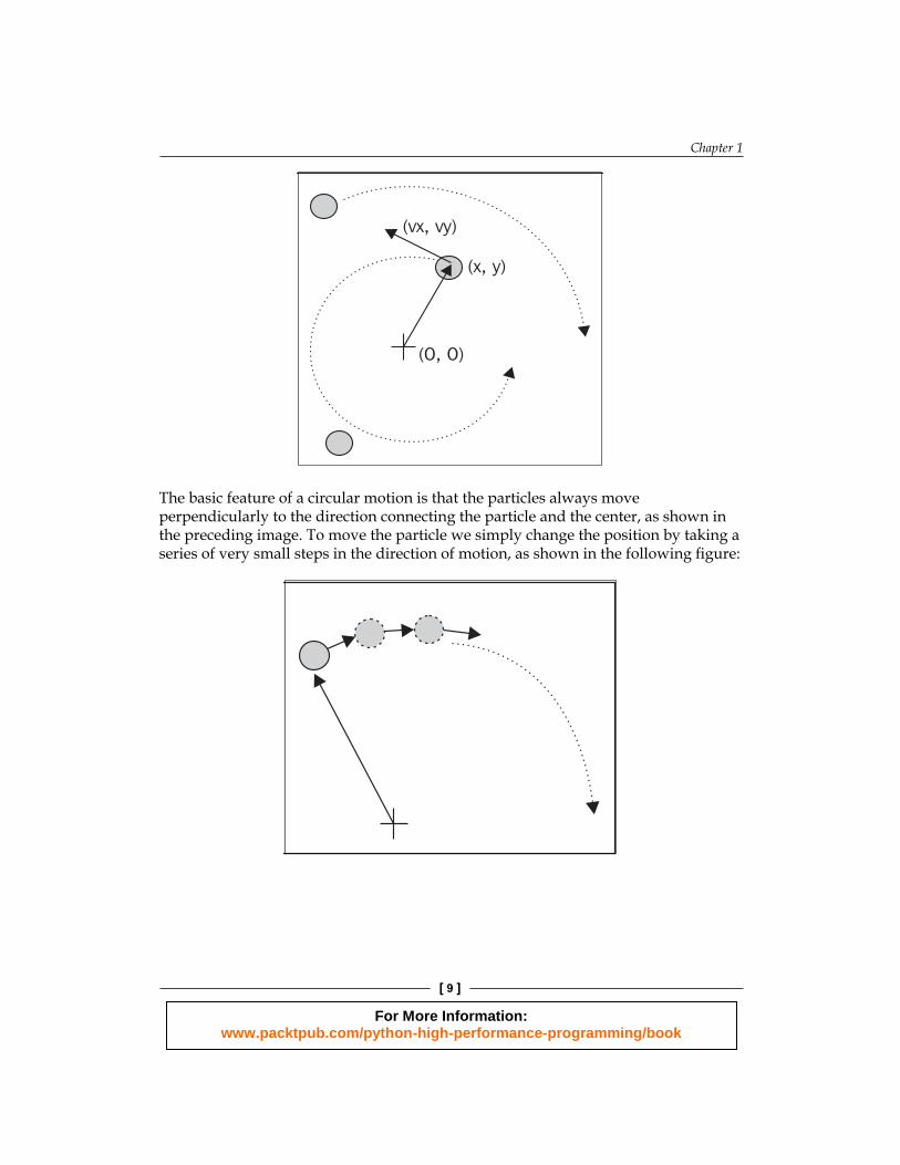
In our fi rst example, we will simulate a system containing particles that constantly rotate around a central point at various speeds, like the hands of a clock.

The necessary information to run our simulation will be the starting positions of the particles, the speed, and the rotation direction. From these elements, we have to calculate the position of the particle in the next instant of time.



Chapter 1

[ 9 ]

(vx, vy)

(x, y)

(0, 0)

The basic feature of a circular motion is that the particles always move perpendicularly to the direction connecting the particle and the center, as shown in the preceding image. To move the particle we simply change the position by taking a series of very small steps in the direction of motion, as shown in the following fi gure:




[ 10 ]

We will start by designing the application in an object-oriented way. According to our requirements, it is natural to have a generic Particle class that simply stores the particle position (x, y) and its angular speed:

class Particle: def __init__(self, x, y, ang_speed): self.x = x self.y = y self.ang_speed = ang_speed

Another class, called ParticleSimulator will encapsulate our laws of motion and will be responsible for changing the positions of the particles over time. The __init__ method will store a list of Particle instances and the evolve method will change the particle positions according to our laws.

We want the particles to rotate around the point (x, y), which, here, is equal to (0, 0), at constant speed. The direction of the particles will always be perpendicular to the direction from the center (refer to the fi rst fi gure of this chapter). To fi nd this vector

v= v ,v( )x y

(corresponding to the Python variables v_x and v_y) it is suffi cient to use these formula e:

v =-yx / x +y2 2

v =xy / x +y2 2

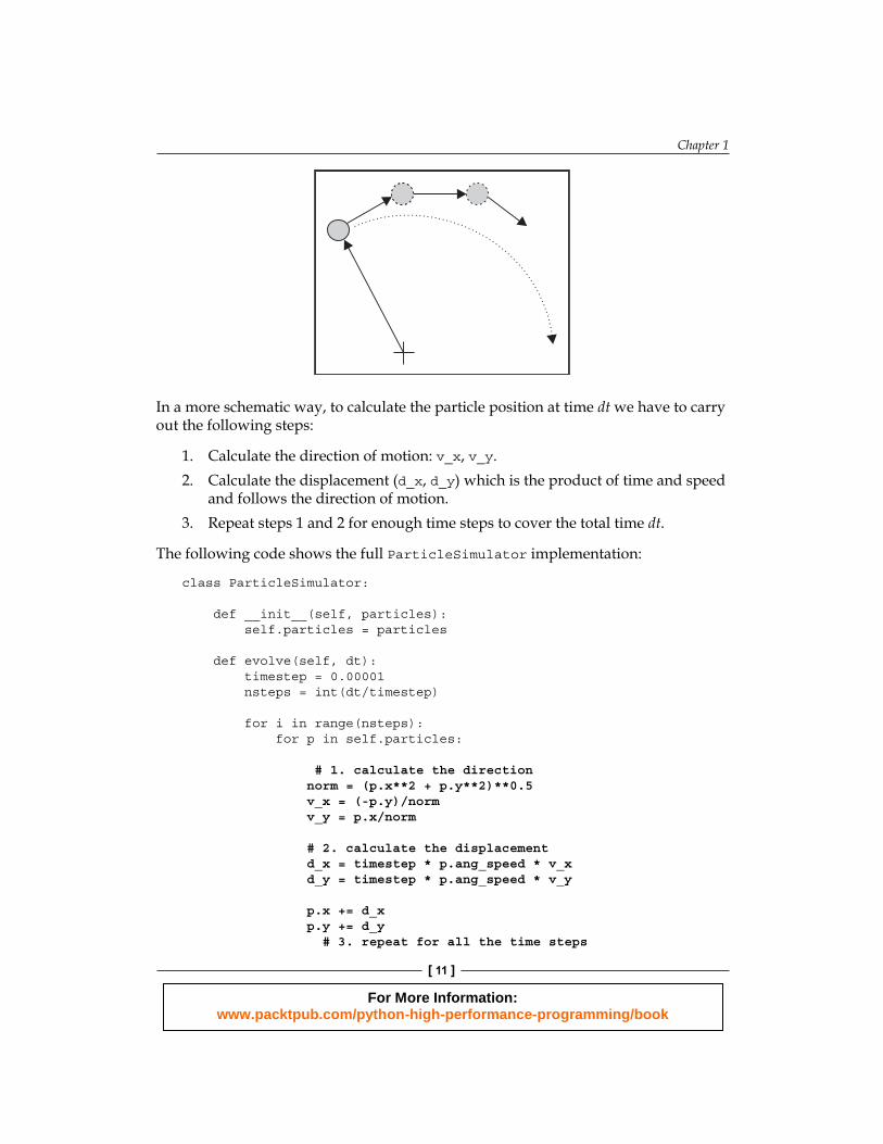
If we let one of our particles move, after a certain time dt, it will follow a circular path, reaching another position. To let the particle follow that trajectory we have to divide the time interval dt into very small time steps where the particle moves tangentially to the circle. The fi nal result, is just an approximation of a circular motion and, in fact, it's similar to a polygon. The time steps should be very small, otherwise the particle trajectory will diverge quickly, as shown in the following fi gure:



Chapter 1

[ 11 ]

In a more schematic way, to calculate the particle position at time dt we have to carry out the following steps:

1. Calculate the direction of motion: v_x, v_y.2. Calculate the displacement (d_x, d_y) which is the product of time and speed

and follows the direction of motion.3. Repeat steps 1 and 2 for enough time steps to cover the total time dt.

The following code shows the full ParticleSimulator implementation:

class ParticleSimulator:

def __init__(self, particles): self.particles = particles

def evolve(self, dt): timestep = 0.00001 nsteps = int(dt/timestep)

for i in range(nsteps): for p in self.particles:

# 1. calculate the direction norm = (p.x**2 + p.y**2)**0.5 v_x = (-p.y)/norm v_y = p.x/norm

# 2. calculate the displacement d_x = timestep * p.ang_speed * v_x d_y = timestep * p.ang_speed * v_y

p.x += d_x p.y += d_y # 3. repeat for all the time steps




[ 12 ]

We can use the matplotlib library to visualize our particles. This library is not included in the Python standard library. To install it, you can follow the instructions included in the offi cial documentation at:

http://matplotlib.org/users/installing.html

Alternatively, you can use the Anaconda Python distribution (https://store.continuum.io/cshop/anaconda/) that includes matplotlib and most of the other third-party packages used in this book. Anaconda is free and available for Linux, Windows, and Mac.

The plot function included in matplotlib can display our particles as points on a Cartesian grid and the FuncAnimation class can animate the evolution of our particles over time.

The visualize function accomplishes this by taking the particle simulator and displaying the trajectory in an animated plot.

The visualize function is structured as follows:

• Setup the axes and display the particles as points using the plot function• Write an initialization function (init) and an update function

(animate) that changes the x, y coordinates of the data points using the line.set_data method

• Create a FuncAnimation instance passing the functions and some parameters• Run the animation with plt.show()

The complete implementation of the visualize function is as follows:from matplotlib import pyplot as pltfrom matplotlib import animation

def visualize(simulator):

X = [p.x for p in simulator.particles] Y = [p.y for p in simulator.particles]

fig = plt.figure() ax = plt.subplot(111, aspect='equal') line, = ax.plot(X, Y, 'ro')

# Axis limits plt.xlim(-1, 1) plt.ylim(-1, 1)



Chapter 1

[ 13 ]

# It will be run when the animation starts def init(): line.set_data([], []) return line,

def animate(i): # We let the particle evolve for 0.1 time units simulator.evolve(0.01) X = [p.x for p in simulator.particles] Y = [p.y for p in simulator.particles]

line.set_data(X, Y) return line,

# Call the animate function each 10 ms anim = animation.FuncAnimation(fig, animate, init_func=init, blit=True,# Efficient animation interval=10) plt.show()

Finally, we defi ne a small test function—test_visualize—that animates a system of three particles rotating in different directions. Note that the third particle completes a round three times faster than the others:

def test_visualize(): particles = [Particle( 0.3, 0.5, +1), Particle( 0.0, -0.5, -1), Particle(-0.1, -0.4, +3)] simulator = ParticleSimulator(particles) visualize(simulator)

if __name__ == '__main__': test_visualize()

Writing tests and benchmarksNow that we have a working simulator, we can start measuring our performance and tuning-up our code, so that our simulator can handle as many particles as possible. The fi rst step in this process is to write a test and a benchmark.

We need a test that checks whether the results produced by the simulation are correct or not. In the optimization process we will rewrite the code to try different solutions; by doing so we may easily introduce bugs. Maintaining a solid test suite is essential to avoid wasting time on broken code.




[ 14 ]

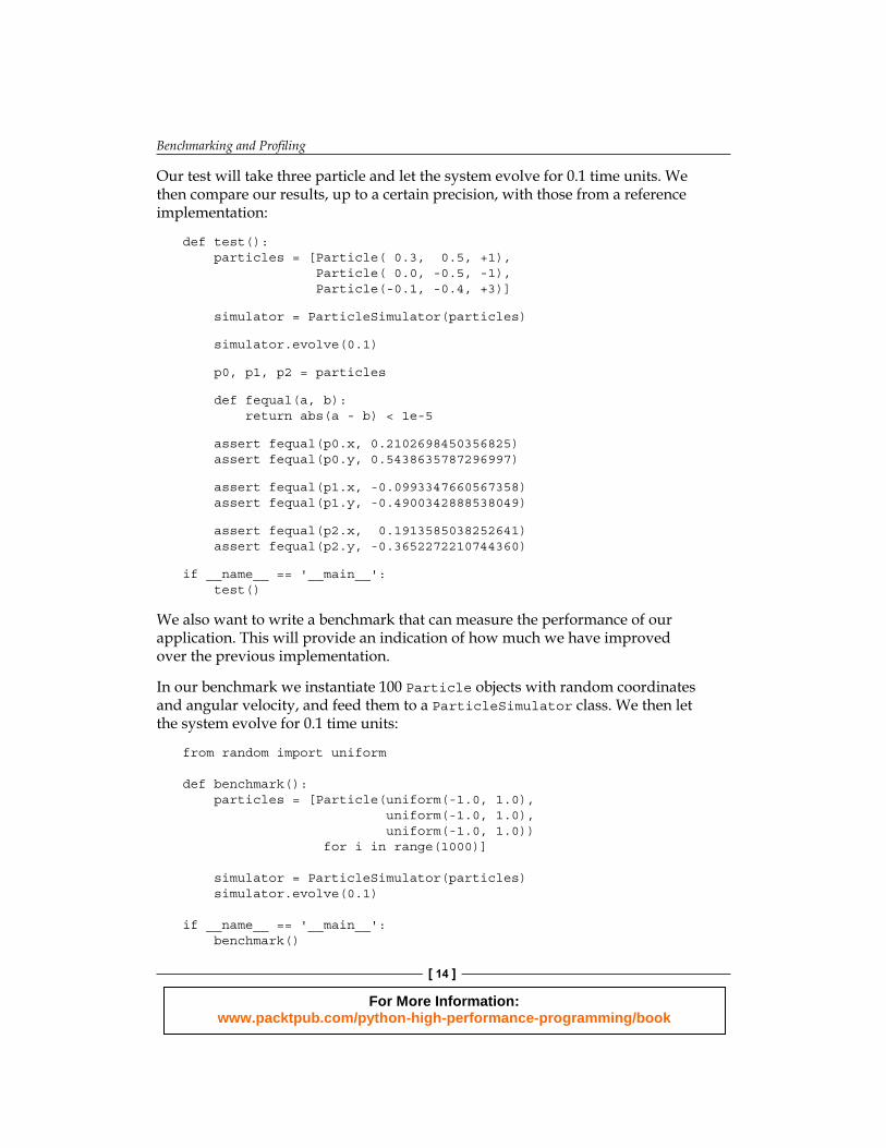
Our test will take three particle and let the system evolve for 0.1 time units. We then compare our results, up to a certain precision, with those from a reference implementation:

def test(): particles = [Particle( 0.3, 0.5, +1), Particle( 0.0, -0.5, -1), Particle(-0.1, -0.4, +3)]

simulator = ParticleSimulator(particles)

simulator.evolve(0.1)

p0, p1, p2 = particles

def fequal(a, b): return abs(a - b) < 1e-5

assert fequal(p0.x, 0.2102698450356825) assert fequal(p0.y, 0.5438635787296997)

assert fequal(p1.x, -0.0993347660567358) assert fequal(p1.y, -0.4900342888538049)

assert fequal(p2.x, 0.1913585038252641) assert fequal(p2.y, -0.3652272210744360)

if __name__ == '__main__': test()

We also want to write a benchmark that can measure the performance of our application. This will provide an indication of how much we have improved over the previous implementation.

In our benchmark we instantiate 100 Particle objects with random coordinates and angular velocity, and feed them to a ParticleSimulator class. We then let the system evolve for 0.1 time units:

from random import uniform

def benchmark(): particles = [Particle(uniform(-1.0, 1.0), uniform(-1.0, 1.0), uniform(-1.0, 1.0)) for i in range(1000)] simulator = ParticleSimulator(particles) simulator.evolve(0.1)

if __name__ == '__main__': benchmark()



Chapter 1

[ 15 ]

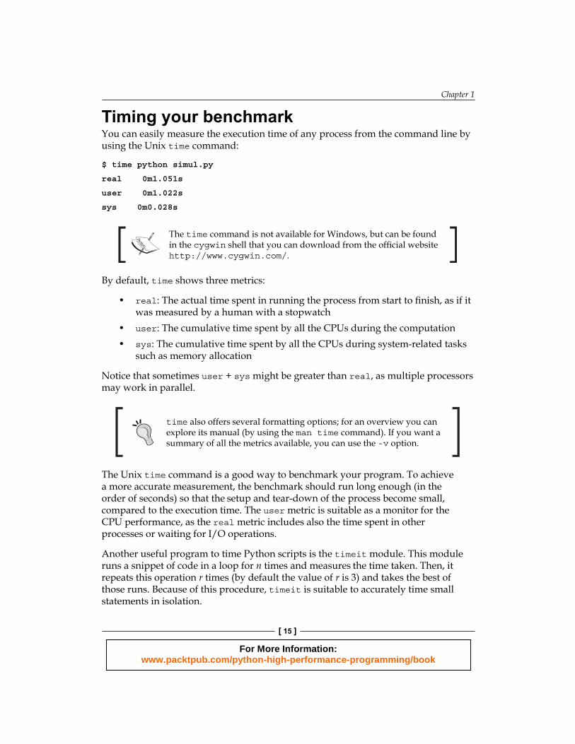
Timing your benchmarkYou can easily measure the execution time of any process from the command line by using the Unix time command:

$ time python simul.py

real 0m1.051s

user 0m1.022s

sys 0m0.028s

The time command is not available for Windows, but can be found in the cygwin shell that you can download from the offi cial website http://www.cygwin.com/.

By default, time shows three metrics:

• real: The actual time spent in running the process from start to fi nish, as if it was measured by a human with a stopwatch

• user: The cumulative time spent by all the CPUs during the computation• sys: The cumulative time spent by all the CPUs during system-related tasks

such as memory allocation

Notice that sometimes user + sys might be greater than real, as multiple processors may work in parallel.

time also offers several formatting options; for an overview you can explore its manual (by using the man time command). If you want a summary of all the metrics available, you can use the -v option.

The Unix time command is a good way to benchmark your program. To achieve a more accurate measurement, the benchmark should run long enough (in the order of seconds) so that the setup and tear-down of the process become small, compared to the execution time. The user metric is suitable as a monitor for the CPU performance, as the real metric includes also the time spent in other processes or waiting for I/O operations.

Another useful program to time Python scripts is the timeit module. This module runs a snippet of code in a loop for n times and measures the time taken. Then, it repeats this operation r times (by default the value of r is 3) and takes the best of those runs. Because of this procedure, timeit is suitable to accurately time small statements in isolation.




[ 16 ]

The timeit module can be used as a Python module, from the command line, or from IPython .

IPython is a Python shell designed for interactive usage. It boosts tab completion and many utilities to time, profi le, and debug your code. We will make use of this shell to try out snippets throughout the book. The IPython shell accepts magic commands—statements that start with a % symbol—that enhance the shell with special behaviors. Commands that start with %% are called cell magics , and these commands can be applied on multi-line snippets (called cells ).

IPython is available on most Linux distributions and is included in Anaconda. You can follow the installation instructions in the offi cial documentation at:

http://ipython.org/install.html

You can use IPython as a regular Python shell (ipython) but it is also available in a Qt-based version (ipython qtconsole) and as a powerful browser-based interface (ipython notebook).

In IPython and command line interfaces it is possible to specify the number of loops or repetitions with the options -n and -r, otherwise they will be determined automatically. When invoking timeit from the command line, you can also give a setup code that will run before executing the statement in a loop.

In the following code we show how to use timeit from IPython, from the command line and as a Python module:

# IPython Interface$ ipythonIn [1]: from simul import benchmarkIn [2]: %timeit benchmark()1 loops, best of 3: 782 ms per loop

# Command Line Interface$ python -m timeit -s 'from simul import benchmark' 'benchmark()'10 loops, best of 3: 826 msec per loop

# Python Interface# put this function into the simul.py script

import timeitresult = timeit.timeit('benchmark()', setup='from __main__ import benchmark', number=10)# result is the time (in seconds) to run the whole loop



Chapter 1

[ 17 ]

result = timeit.repeat('benchmark()', setup='from __main__ import benchmark', number=10, repeat=3)# result is a list containing the time of each repetition (repeat=3 in this case)

Notice that while the command line and IPython interfaces are automatically determining a reasonable value for n, the Python interface requires you to explicitly pass it as the number argument.

Finding bottlenecks with cProfi leAfter assessing the execution time of the program we are ready to identify the parts of the code that need performance tuning. Those parts are typically quite small, compared to the size of the program.

Historically, there are three different profi ling modules in Python's standard library:

• The profile module: This module is written in pure Python and adds a signifi cant overhead to the program execution. Its presence in the standard library is due mainly to its extendibility.

• The hotshot module: A C module designed to minimize the profi ling overhead. Its use is not recommended by the Python community and it is not available in Python 3.

• The cProfile module: The main profi ling module, with an interface similar to profile. It has a small overhead and it is suitable as a general purpose profi ler.

We will see how to use the cProfi le module in two different ways:

• From the command line• From IPython

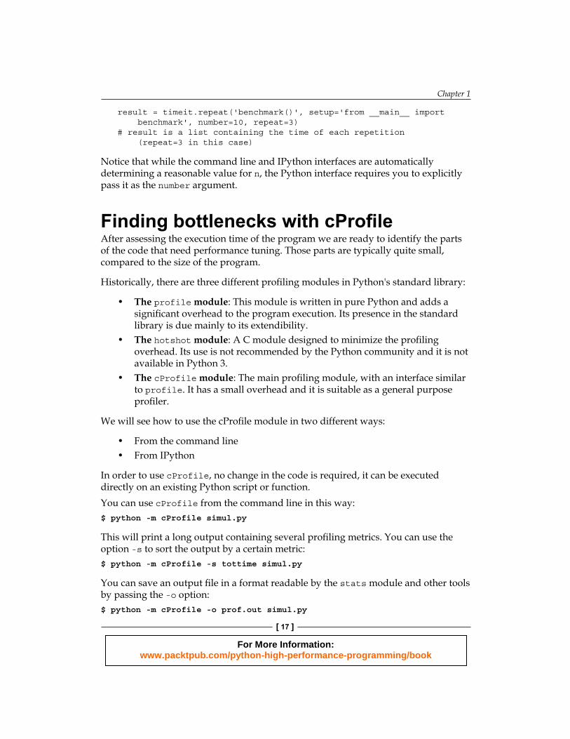
In order to use cProfile, no change in the code is required, it can be executed directly on an existing Python script or function.You can use cProfile from the command line in this way:$ python -m cProfile simul.py

This will print a long output containing several profi ling metrics. You can use the option -s to sort the output by a certain metric:$ python -m cProfile -s tottime simul.py

You can save an output fi le in a format readable by the stats module and other tools by passing the -o option:$ python -m cProfile -o prof.out simul.py




[ 18 ]

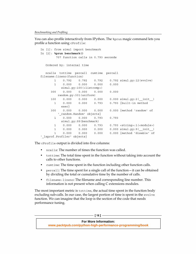
You can also profi le interactively from IPython. The %prun magic command lets you profi le a function using cProfile:

In [1]: from simul import benchmarkIn [2]: %prun benchmark() 707 function calls in 0.793 seconds

Ordered by: internal time

ncalls tottime percall cumtime percall filename:lineno(function) 1 0.792 0.792 0.792 0.792 simul.py:12(evolve) 1 0.000 0.000 0.000 0.000 simul.py:100(<listcomp>) 300 0.000 0.000 0.000 0.000 random.py:331(uniform) 100 0.000 0.000 0.000 0.000 simul.py:2(__init__) 1 0.000 0.000 0.793 0.793 {built-in method exec} 300 0.000 0.000 0.000 0.000 {method 'random' of '_random.Random' objects} 1 0.000 0.000 0.793 0.793 simul.py:99(benchmark) 1 0.000 0.000 0.793 0.793 <string>:1(<module>) 1 0.000 0.000 0.000 0.000 simul.py:9(__init__) 1 0.000 0.000 0.000 0.000 {method 'disable' of '_lsprof.Profiler' objects}

The cProfile output is divided into fi ve columns:

• ncalls: The number of times the function was called.• tottime: The total time spent in the function without taking into account the

calls to other functions.• cumtime: The time spent in the function including other function calls.• percall: The time spent for a single call of the function—it can be obtained

by dividing the total or cumulative time by the number of calls.• filename:lineno: The fi lename and corresponding line number. This

information is not present when calling C extensions modules.

The most important metric is tottime, the actual time spent in the function body excluding sub-calls. In our case, the largest portion of time is spent in the evolve function. We can imagine that the loop is the section of the code that needs performance tuning.



Chapter 1

[ 19 ]

Analyzing data in a textual way can be daunting for big programs with a lot of calls and sub-calls. Some graphic tools aid the task by improving the navigation with an interactive interface.

KCachegrind is a GUI (Graphical User Interface) useful to analyze the profi ling output of different programs.

KCachegrind is available in Ubuntu 13.10 offi cial repositories. The Qt port, QCacheGrind can be downloaded for Windows from the following web page:http://sourceforge.net/projects/qcachegrindwin/

Mac users can compile QCacheGrind using Mac Ports (http://www.macports.org/) by following the instructions present in the blog post at this link:http://blogs.perl.org/users/rurban/2013/04/install-kachegrind-on-macosx-with-ports.html

KCachegrind can't read directly the output fi les produced by cProfile. Luckily, the pyprof2calltree third-party Python module is able to convert the cProfile output fi le into a format readable by KCachegrind.You can install pyprof2calltree from source (https://pypi.python.org/pypi/pyprof2calltree/) or from the Python Package Index (https://pypi.python.org/).

To best show the KCachegrind features we will use another example with a more diversifi ed structure. We defi ne a recursive function factorial, and two other functions that use factorial, and they are taylor_exp and taylor_sin. They represent the polynomial coeffi cients of the Taylor approximations of exp(x) and sin(x):

def factorial(n): if n == 0: return 1.0 else: return float(n) * factorial(n-1)

def taylor_exp(n): return [1.0/factorial(i) for i in range(n)]

def taylor_sin(n): res = [] for i in range(n): if i % 2 == 1:




[ 20 ]

res.append((-1)**((i-1)/2)/float(factorial(i))) else: res.append(0.0) return res

def benchmark(): taylor_exp(500) taylor_sin(500)

if __name__ == '__main__': benchmark()

We need to fi rst generate the cProfile output fi le:

$ python -m cProfile -o prof.out taylor.py

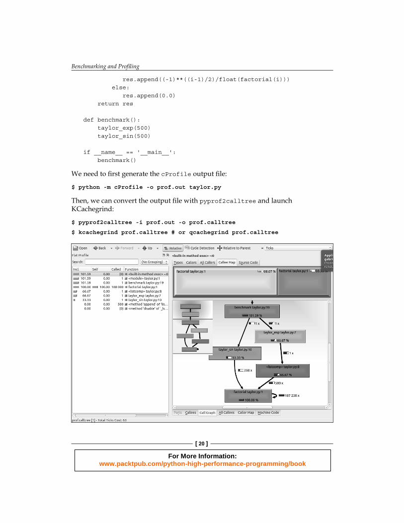
Then, we can convert the output fi le with pyprof2calltree and launch KCachegrind:

$ pyprof2calltree -i prof.out -o prof.calltree

$ kcachegrind prof.calltree # or qcachegrind prof.calltree



Chapter 1

[ 21 ]

The preceding image is a screenshot of the KCachegrind user interface. On the left we have an output fairly similar to cProfile. The actual column names are slightly different: Incl. translates to cProfile module's cumtime; Self translates to tottime. The values are given in percentages by clicking on the Relative button on the menu bar. By clicking on the column headers you can sort by the corresponding property.

On the top right, a click on the Callee Map tab contains a diagram of the function costs. In the diagram, each function is represented by a rectangle and the time percentage spent by the function is proportional to the area of the rectangle. Rectangles can contain sub-rectangles that represent sub-calls to other functions. In this case, we can easily see that there are two rectangles for the factorial function. The one on the left corresponds to the calls made by taylor_exp and the one on the right to the calls made by taylor_sin.

On the bottom right, you can display another diagram—the call graph—by clicking on the Call Graph tab. A call graph is a graphical representation of the calling relationship between the functions: each square represents a function and the arrows imply a calling relationship. For example, taylor_exp calls <listcomp> (a list comprehension) which calls factorial 500 times taylor_sin calls factorial 250 times. KCachegrind also detects recursive calls: factorial calls itself 187250 times.

You can navigate to the Call Graph or the Caller Map tabs by double-clicking on the rectangles; the interface will update accordingly showing that the timing properties are relative to the selected function. For example, double-clicking on taylor_exp will cause the graph to change, showing only the taylor_exp contribution to the total cost.

Gprof2Dot (https://code.google.com/p/jrfonseca/wiki/Gprof2Dot) is another popular tool used to produce call graphs. Starting from output fi les produced by one of the supported profi lers, it will generate a .dot diagram representing the call graph.

Profi le line by line with line_profi lerNow that we know which function we have to optimize, we can use the line_profiler module that shows us how time is spent in a line-by-line fashion. This is very useful in situations where it's diffi cult to determine which statements are costly. The line_profiler module is a third-party module that is available on the Python Package Index and can be installed by following the instructions on its website:

http://pythonhosted.org/line_profiler/




[ 22 ]

In order to use line_profiler, we need to apply a @profile decorator to the functions we intend to monitor. Notice that you don't have to import the profile function from another module, as it gets injected in the global namespace when running the profi ling script kernprof.py. To produce profi ling output for our program we need to add the @profile decorator to the evolve function:

@profiledef evolve: # code

The script kernprof.py will produce an output fi le and will print on standard output the result of the profi ling. We should run the script with two options:

• -l to use the line_profiler function• -v to immediately print the results on screen

$ kernprof.py -l -v simul.py

It is also possible to run the profi ler in an IPython shell for interactive editing. You should fi rst load the line_profiler extension that will provide the magic command lprun. By using that command you can avoid adding the @profile decorator.

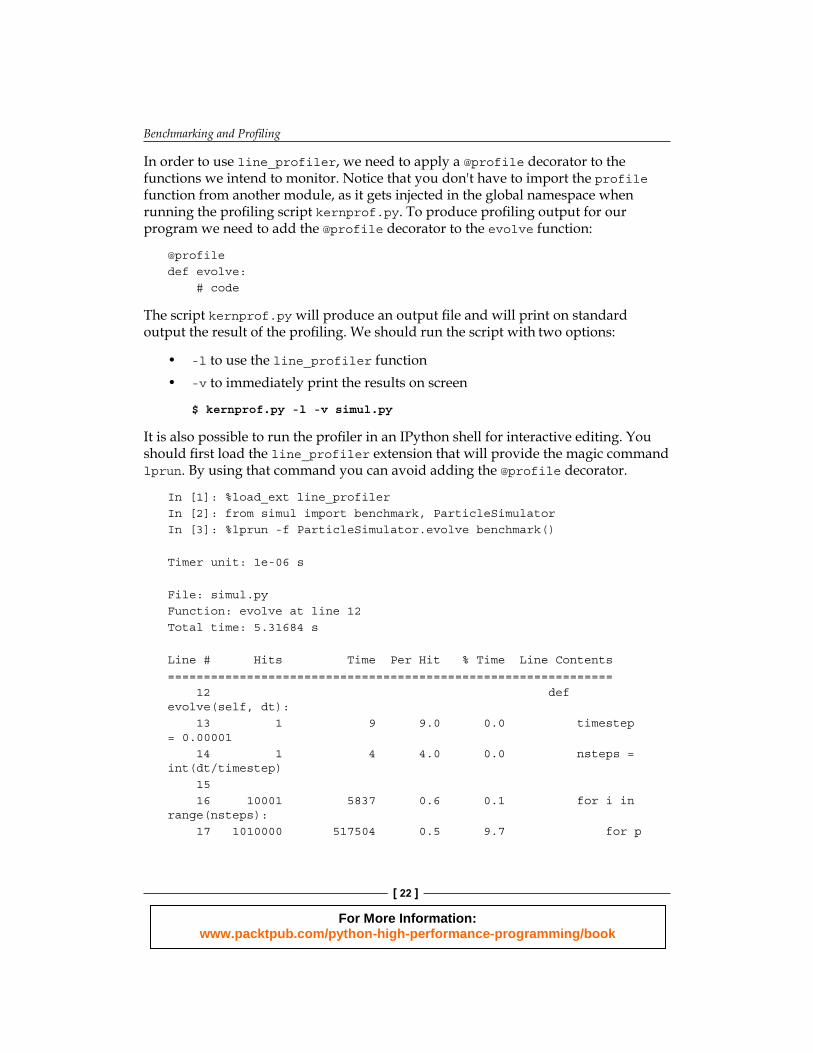
In [1]: %load_ext line_profilerIn [2]: from simul import benchmark, ParticleSimulatorIn [3]: %lprun -f ParticleSimulator.evolve benchmark() Timer unit: 1e-06 s

File: simul.pyFunction: evolve at line 12Total time: 5.31684 s

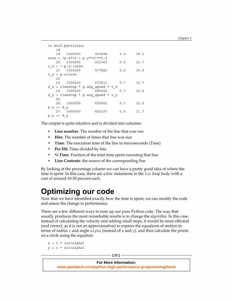
Line # Hits Time Per Hit % Time Line Contents============================================================== 12 def evolve(self, dt): 13 1 9 9.0 0.0 timestep = 0.00001 14 1 4 4.0 0.0 nsteps = int(dt/timestep) 15 16 10001 5837 0.6 0.1 for i in range(nsteps): 17 1010000 517504 0.5 9.7 for p



Chapter 1

[ 23 ]

in self.particles: 18 19 1000000 963498 1.0 18.1 norm = (p.x**2 + p.y**2)**0.5 20 1000000 621063 0.6 11.7 v_x = (-p.y)/norm 21 1000000 577882 0.6 10.9 v_y = p.x/norm 22 23 1000000 672811 0.7 12.7 d_x = timestep * p.ang_speed * v_x 24 1000000 685092 0.7 12.9 d_y = timestep * p.ang_speed * v_y 25 26 1000000 650802 0.7 12.2 p.x += d_x 27 1000000 622337 0.6 11.7 p.y += d_y

The output is quite intuitive and is divided into columns:

• Line number: The number of the line that was run• Hits: The number of times that line was run• Time: The execution time of the line in microseconds (Time)• Per Hit: Time divided by hits• % Time: Fraction of the total time spent executing that line• Line Contents: the source of the corresponding line

By looking at the percentage column we can have a pretty good idea of where the time is spent. In this case, there are a few statements in the for loop body with a cost of around 10-20 percent each.

Optimizing our codeNow that we have identifi ed exactly how the time is spent, we can modify the code and assess the change in performance.

There are a few different ways to tune up our pure Python code. The way that usually produces the most remarkable results is to change the algorithm. In this case, instead of calculating the velocity and adding small steps, it would be more effi cient (and correct, as it is not an approximation) to express the equations of motion in terms of radius r and angle alpha (instead of x and y), and then calculate the points on a circle using the equation:

x = r * cos(alpha)y = r * sin(alpha)




[ 24 ]

Another way lies in minimizing the number of instructions. For example, we can pre-calculate the factor timestep * p.ang_speed that doesn't change with time. We can exchange the loop order (fi rst we iterate on particles, then we iterate on time steps) and put the calculation of the factor outside of the loop on the particles.

The line by line profi ling showed also that even simple assignment operations can take a considerable amount of time. For example, the following statement takes more than 10 percent of the total time:

v_x = (-p.y)/norm

Therefore, a way to optimize the loop is reducing the number of assignment operations. To do that, we can avoid intermediate variables by sacrifi cing readability and rewriting the expression in a single and slightly more complex statement (notice that the right-hand side gets evaluated completely before being assigned to the variables):

p.x, p.y = p.x - t_x_ang*p.y/norm, p.y + t_x_ang * p.x/norm

This leads to the following code:

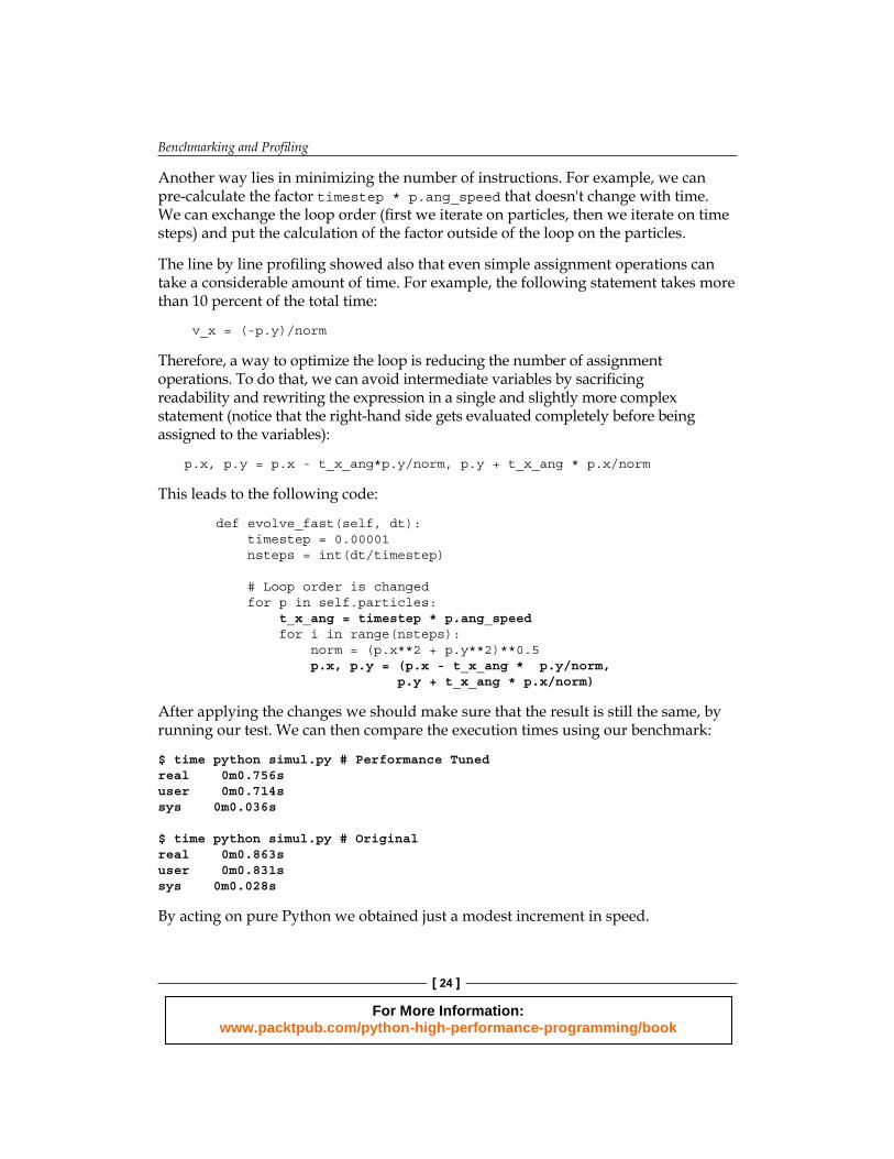
def evolve_fast(self, dt): timestep = 0.00001 nsteps = int(dt/timestep) # Loop order is changed for p in self.particles: t_x_ang = timestep * p.ang_speed for i in range(nsteps): norm = (p.x**2 + p.y**2)**0.5 p.x, p.y = (p.x - t_x_ang * p.y/norm, p.y + t_x_ang * p.x/norm)

After applying the changes we should make sure that the result is still the same, by running our test. We can then compare the execution times using our benchmark:

$ time python simul.py # Performance Tunedreal 0m0.756suser 0m0.714ssys 0m0.036s

$ time python simul.py # Originalreal 0m0.863suser 0m0.831ssys 0m0.028s

By acting on pure Python we obtained just a modest increment in speed.



Chapter 1

[ 25 ]

The dis moduleSometimes, it's not easy to evaluate how many operations a Python statement will take. In this section, we will explore Python internals to estimate the performance of Python statements. Python code gets converted to an intermediate representation—called bytecode—that gets executed by the Python virtual machine.

To help inspect how the code gets converted into bytecode we can use the Python module dis (disassemble). Its usage is really simple, it is suffi cient to call the function dis.dis on the ParticleSimulator.evolve method:

import disfrom simul import ParticleSimulatordis.dis(ParticleSimulator.evolve)

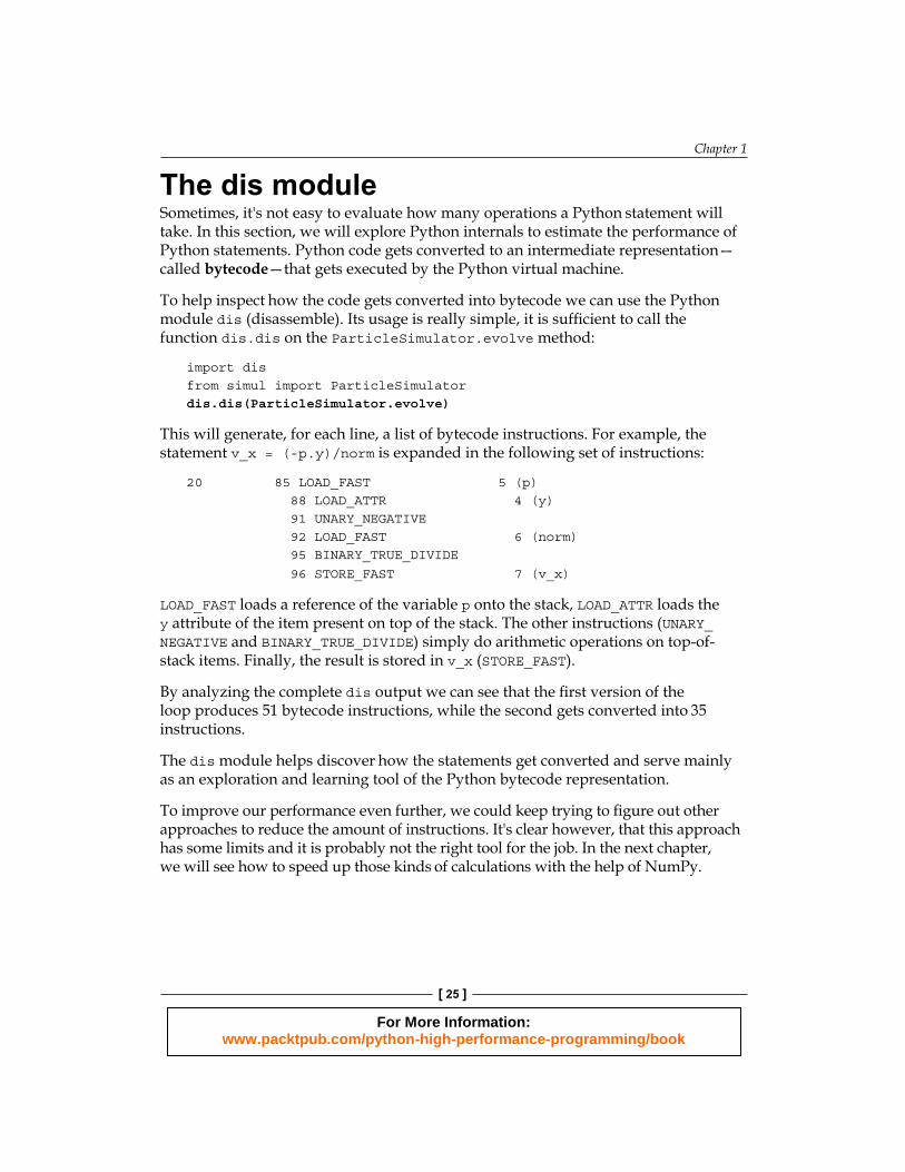
This will generate, for each line, a list of bytecode instructions. For example, the statement v_x = (-p.y)/norm is expanded in the following set of instructions:

20 85 LOAD_FAST 5 (p) 88 LOAD_ATTR 4 (y) 91 UNARY_NEGATIVE 92 LOAD_FAST 6 (norm) 95 BINARY_TRUE_DIVIDE

96 STORE_FAST 7 (v_x)

LOAD_FAST loads a reference of the variable p onto the stack, LOAD_ATTR loads the y attribute of the item present on top of the stack. The other instructions (UNARY_NEGATIVE and BINARY_TRUE_DIVIDE) simply do arithmetic operations on top-of-stack items. Finally, the result is stored in v_x (STORE_FAST).

By analyzing the complete dis output we can see that the fi rst version of the loop produces 51 bytecode instructions, while the second gets converted into 35 instructions.

The dis module helps discover how the statements get converted and serve mainly as an exploration and learning tool of the Python bytecode representation.

To improve our performance even further, we could keep trying to fi gure out other approaches to reduce the amount of instructions. It's clear however, that this approach has some limits and it is probably not the right tool for the job. In the next chapter, we will see how to speed up those kinds of calculations with the help of NumPy.




[ 26 ]

Profi ling memory usage with memory_profi lerIn some cases, memory usage constitutes an issue. For example, if we want to handle a huge number of particles we will have a memory overhead due to the creation of many Particle instances.

The module memory_profiler summarizes, in a way similar to line_profiler, the memory usage of the process.

The memory_profiler package is also available on the Python Package Index. You should also install the psutil module (https://code.google.com/p/psutil/) as an optional dependency, it will make memory_profiler run considerably faster.

Just like line_profiler, memory_profiler also requires the instrumentation of the source code, by putting a @profile decorator on the function we intend to monitor. In our case, we want to analyze the function benchmark.

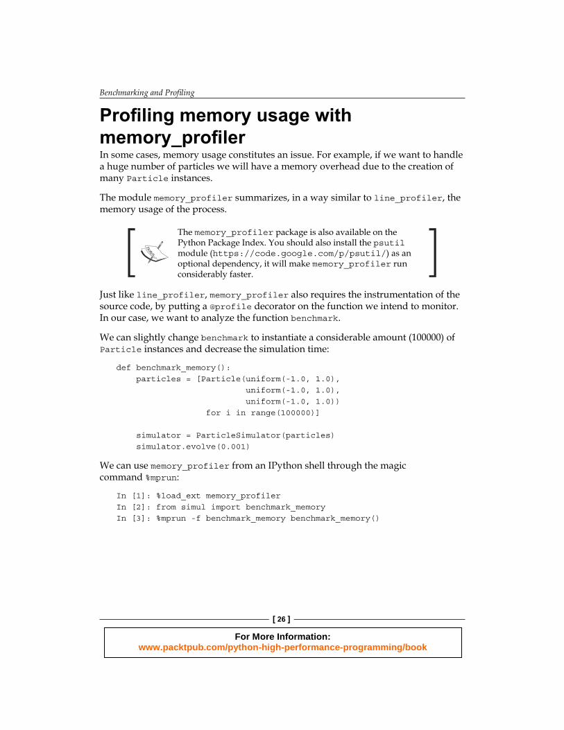
We can slightly change benchmark to instantiate a considerable amount (100000) of Particle instances and decrease the simulation time:

def benchmark_memory(): particles = [Particle(uniform(-1.0, 1.0), uniform(-1.0, 1.0), uniform(-1.0, 1.0)) for i in range(100000)] simulator = ParticleSimulator(particles) simulator.evolve(0.001)

We can use memory_profiler from an IPython shell through the magic command %mprun:

In [1]: %load_ext memory_profilerIn [2]: from simul import benchmark_memoryIn [3]: %mprun -f benchmark_memory benchmark_memory()



Chapter 1

[ 27 ]

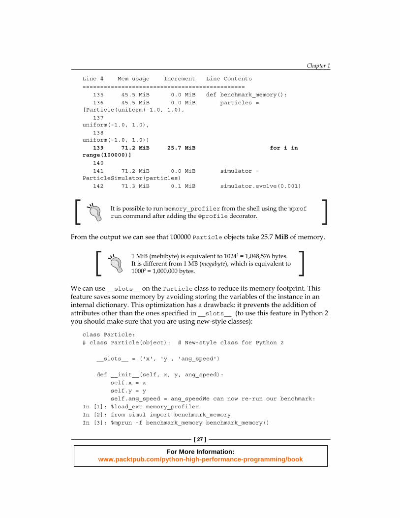
Line # Mem usage Increment Line Contents============================================== 135 45.5 MiB 0.0 MiB def benchmark_memory(): 136 45.5 MiB 0.0 MiB particles = [Particle(uniform(-1.0, 1.0), 137 uniform(-1.0, 1.0), 138 uniform(-1.0, 1.0)) 139 71.2 MiB 25.7 MiB for i in range(100000)] 140 141 71.2 MiB 0.0 MiB simulator = ParticleSimulator(particles) 142 71.3 MiB 0.1 MiB simulator.evolve(0.001)

It is possible to run memory_profiler from the shell using the mprof run command after adding the @profile decorator.

From the output we can see that 100000 Particle objects take 25.7 MiB of memory.

1 MiB (mebibyte) is equivalent to 10242 = 1,048,576 bytes. It is different from 1 MB (megabyte), which is equivalent to 10002 = 1,000,000 bytes.

We can use __slots__ on the Particle class to reduce its memory footprint. This feature saves some memory by avoiding storing the variables of the instance in an internal dictionary. This optimization has a drawback: it prevents the addition of attributes other than the ones specifi ed in __slots__ (to use this feature in Python 2 you should make sure that you are using new-style classes):

class Particle: # class Particle(object): # New-style class for Python 2

__slots__ = ('x', 'y', 'ang_speed') def __init__(self, x, y, ang_speed): self.x = x self.y = y self.ang_speed = ang_speedWe can now re-run our benchmark:In [1]: %load_ext memory_profilerIn [2]: from simul import benchmark_memoryIn [3]: %mprun -f benchmark_memory benchmark_memory()




[ 28 ]

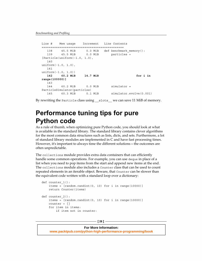
Line # Mem usage Increment Line Contents============================================== 138 45.5 MiB 0.0 MiB def benchmark_memory(): 139 45.5 MiB 0.0 MiB particles = [Particle(uniform(-1.0, 1.0), 140 uniform(-1.0, 1.0), 141 uniform(-1.0, 1.0)) 142 60.2 MiB 14.7 MiB for i in range(100000)] 143 144 60.2 MiB 0.0 MiB simulator = ParticleSimulator(particles) 145 60.3 MiB 0.1 MiB simulator.evolve(0.001)

By rewriting the Particle class using __slots__ we can save 11 MiB of memory.

Performance tuning tips for pure Python codeAs a rule of thumb, when optimizing pure Python code, you should look at what is available in the standard library. The standard library contains clever algorithms for the most common data structures such as lists, dicts, and sets. Furthermore, a lot of standard library modules are implemented in C and have fast processing times. However, it's important to always time the different solutions—the outcomes are often unpredictable.

The collections module provides extra data containers that can effi ciently handle some common operations. For example, you can use deque in place of a list when you need to pop items from the start and append new items at the end. The collections module also includes a Counter class that can be used to count repeated elements in an iterable object. Beware, that Counter can be slower than the equivalent code written with a standard loop over a dictionary:

def counter_1(): items = [random.randint(0, 10) for i in range(10000)] return Counter(items)

def counter_2(): items = [random.randint(0, 10) for i in range(10000)] counter = {} for item in items: if item not in counter:



Chapter 1

[ 29 ]

counter[item] = 0 else: counter[item] += 1 return counter

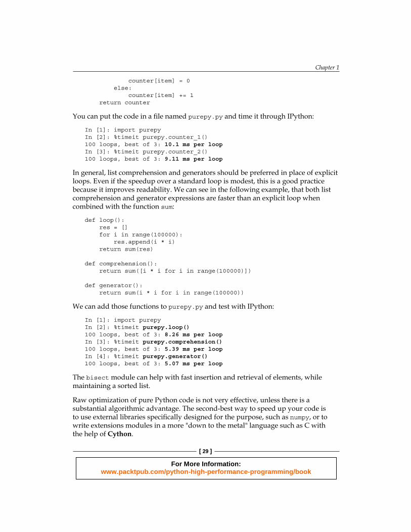
You can put the code in a fi le named purepy.py and time it through IPython:

In [1]: import purepyIn [2]: %timeit purepy.counter_1()100 loops, best of 3: 10.1 ms per loopIn [3]: %timeit purepy.counter_2()100 loops, best of 3: 9.11 ms per loop

In general, list comprehension and generators should be preferred in place of explicit loops. Even if the speedup over a standard loop is modest, this is a good practice because it improves readability. We can see in the following example, that both list comprehension and generator expressions are faster than an explicit loop when combined with the function sum:

def loop(): res = [] for i in range(100000): res.append(i * i) return sum(res)

def comprehension(): return sum([i * i for i in range(100000)])

def generator(): return sum(i * i for i in range(100000))

We can add those functions to purepy.py and test with IPython:

In [1]: import purepyIn [2]: %timeit purepy.loop()100 loops, best of 3: 8.26 ms per loopIn [3]: %timeit purepy.comprehension()100 loops, best of 3: 5.39 ms per loopIn [4]: %timeit purepy.generator()100 loops, best of 3: 5.07 ms per loop

The bisect module can help with fast insertion and retrieval of elements, while maintaining a sorted list.

Raw optimization of pure Python code is not very effective, unless there is a substantial algorithmic advantage. The second-best way to speed up your code is to use external libraries specifi cally designed for the purpose, such as numpy, or to write extensions modules in a more "down to the metal" language such as C with the help of Cython.




[ 30 ]

SummaryIn this chapter, we introduced the basic principles of optimization and we applied those principles to our test application. The most important thing is identifying the bottlenecks in the application before editing the code. We saw how to write and time a benchmark using the time Unix command and the Python timeit module. We learned how to profi le our application using cProfile, line_profiler, and memory_profiler, and how to analyze and navigate graphically the profi ling data with KCachegrind. We surveyed some of the strategies to optimize pure Python code by leveraging the tools available in the standard library.

In the next chapter, we will see how to use numpy to dramatically speedup computations in an easy and convenient way.



Where to buy this book You can buy Python High Performance Programming from the Packt Publishing website:

.

Free shipping to the US, UK, Europe and selected Asian countries. For more information, please

read our shipping policy.

Alternatively, you can buy the book from Amazon, BN.com, Computer Manuals and

most internet book retailers.

www.PacktPub.com


http://www.packtpub.com/Shippingpolicy

http://www.packtpub.com/


Python High Performance Programming - Packt · Python High Performance Programming Gabriele Lanaro...

Documents

Transcript of Python High Performance Programming - Packt · Python High Performance Programming Gabriele Lanaro...