Python for Data Analysis
470
-
Upload
wes-mckinney -
Category
Documents
-
view
358 -
download
18
Transcript of Python for Data Analysis


Python for Data Analysis
Wes McKinney
Beijing • Cambridge • Farnham • Köln • Sebastopol • Tokyo

Python for Data Analysisby Wes McKinney
Copyright © 2013 Wes McKinney. All rights reserved.Printed in the United States of America.
Published by O’Reilly Media, Inc., 1005 Gravenstein Highway North, Sebastopol, CA 95472.
O’Reilly books may be purchased for educational, business, or sales promotional use. Online editionsare also available for most titles (http://my.safaribooksonline.com). For more information, contact ourcorporate/institutional sales department: 800-998-9938 or [email protected].
Editors: Julie Steele and Meghan BlanchetteProduction Editor: Melanie YarbroughCopyeditor: Teresa ExleyProofreader: BIM Publishing Services
Indexer: BIM Publishing ServicesCover Designer: Karen MontgomeryInterior Designer: David FutatoIllustrator: Rebecca Demarest
October 2012: First Edition.
Revision History for the First Edition:2012-10-05 First release
See http://oreilly.com/catalog/errata.csp?isbn=9781449319793 for release details.
Nutshell Handbook, the Nutshell Handbook logo, and the O’Reilly logo are registered trademarks ofO’Reilly Media, Inc. Python for Data Analysis, the cover image of a golden-tailed tree shrew, and relatedtrade dress are trademarks of O’Reilly Media, Inc.
Many of the designations used by manufacturers and sellers to distinguish their products are claimed astrademarks. Where those designations appear in this book, and O’Reilly Media, Inc., was aware of atrademark claim, the designations have been printed in caps or initial caps.
While every precaution has been taken in the preparation of this book, the publisher and author assumeno responsibility for errors or omissions, or for damages resulting from the use of the information con-tained herein.
ISBN: 978-1-449-31979-3
[LSI]
1349356084

Table of Contents
Preface . . . . . . . . . . . . . . . . . . . . . . . . . . . . . . . . . . . . . . . . . . . . . . . . . . . . . . . . . . . . . . . . . . . . . xi
1. Preliminaries . . . . . . . . . . . . . . . . . . . . . . . . . . . . . . . . . . . . . . . . . . . . . . . . . . . . . . . . . . . 1What Is This Book About? 1Why Python for Data Analysis? 2
Python as Glue 2Solving the “Two-Language” Problem 2Why Not Python? 3
Essential Python Libraries 3NumPy 4pandas 4matplotlib 5IPython 5SciPy 6
Installation and Setup 6Windows 7Apple OS X 9GNU/Linux 10Python 2 and Python 3 11Integrated Development Environments (IDEs) 11
Community and Conferences 12Navigating This Book 12
Code Examples 13Data for Examples 13Import Conventions 13Jargon 13
Acknowledgements 14
2. Introductory Examples . . . . . . . . . . . . . . . . . . . . . . . . . . . . . . . . . . . . . . . . . . . . . . . . . . 171.usa.gov data from bit.ly 17
Counting Time Zones in Pure Python 19
iii

Counting Time Zones with pandas 21MovieLens 1M Data Set 26
Measuring rating disagreement 30US Baby Names 1880-2010 32
Analyzing Naming Trends 36Conclusions and The Path Ahead 43
3. IPython: An Interactive Computing and Development Environment . . . . . . . . . . . . 45IPython Basics 46
Tab Completion 47Introspection 48The %run Command 49Executing Code from the Clipboard 50Keyboard Shortcuts 52Exceptions and Tracebacks 53Magic Commands 54Qt-based Rich GUI Console 55Matplotlib Integration and Pylab Mode 56
Using the Command History 58Searching and Reusing the Command History 58Input and Output Variables 58Logging the Input and Output 59
Interacting with the Operating System 60Shell Commands and Aliases 60Directory Bookmark System 62
Software Development Tools 62Interactive Debugger 62Timing Code: %time and %timeit 67Basic Profiling: %prun and %run -p 68Profiling a Function Line-by-Line 70
IPython HTML Notebook 72Tips for Productive Code Development Using IPython 72
Reloading Module Dependencies 74Code Design Tips 74
Advanced IPython Features 76Making Your Own Classes IPython-friendly 76Profiles and Configuration 77
Credits 78
4. NumPy Basics: Arrays and Vectorized Computation . . . . . . . . . . . . . . . . . . . . . . . . . . 79The NumPy ndarray: A Multidimensional Array Object 80
Creating ndarrays 81Data Types for ndarrays 83
iv | Table of Contents

Operations between Arrays and Scalars 85Basic Indexing and Slicing 86Boolean Indexing 89Fancy Indexing 92Transposing Arrays and Swapping Axes 93
Universal Functions: Fast Element-wise Array Functions 95Data Processing Using Arrays 97
Expressing Conditional Logic as Array Operations 98Mathematical and Statistical Methods 100Methods for Boolean Arrays 101Sorting 101Unique and Other Set Logic 102
File Input and Output with Arrays 103Storing Arrays on Disk in Binary Format 103Saving and Loading Text Files 104
Linear Algebra 105Random Number Generation 106Example: Random Walks 108
Simulating Many Random Walks at Once 109
5. Getting Started with pandas . . . . . . . . . . . . . . . . . . . . . . . . . . . . . . . . . . . . . . . . . . . . 111Introduction to pandas Data Structures 112
Series 112DataFrame 115Index Objects 120
Essential Functionality 122Reindexing 122Dropping entries from an axis 125Indexing, selection, and filtering 125Arithmetic and data alignment 128Function application and mapping 132Sorting and ranking 133Axis indexes with duplicate values 136
Summarizing and Computing Descriptive Statistics 137Correlation and Covariance 139Unique Values, Value Counts, and Membership 141
Handling Missing Data 142Filtering Out Missing Data 143Filling in Missing Data 145
Hierarchical Indexing 147Reordering and Sorting Levels 149Summary Statistics by Level 150Using a DataFrame’s Columns 150
Table of Contents | v

Other pandas Topics 151Integer Indexing 151Panel Data 152
6. Data Loading, Storage, and File Formats . . . . . . . . . . . . . . . . . . . . . . . . . . . . . . . . . . 155Reading and Writing Data in Text Format 155
Reading Text Files in Pieces 160Writing Data Out to Text Format 162Manually Working with Delimited Formats 163JSON Data 165XML and HTML: Web Scraping 166
Binary Data Formats 171Using HDF5 Format 171Reading Microsoft Excel Files 172
Interacting with HTML and Web APIs 173Interacting with Databases 174
Storing and Loading Data in MongoDB 176
7. Data Wrangling: Clean, Transform, Merge, Reshape . . . . . . . . . . . . . . . . . . . . . . . . 177Combining and Merging Data Sets 177
Database-style DataFrame Merges 178Merging on Index 182Concatenating Along an Axis 185Combining Data with Overlap 188
Reshaping and Pivoting 189Reshaping with Hierarchical Indexing 190Pivoting “long” to “wide” Format 192
Data Transformation 194Removing Duplicates 194Transforming Data Using a Function or Mapping 195Replacing Values 196Renaming Axis Indexes 197Discretization and Binning 199Detecting and Filtering Outliers 201Permutation and Random Sampling 202Computing Indicator/Dummy Variables 203
String Manipulation 205String Object Methods 206Regular expressions 207Vectorized string functions in pandas 210
Example: USDA Food Database 212
vi | Table of Contents
8. Plotting and Visualization . . . . . . . . . . . . . . . . . . . . . . . . . . . . . . . . . . . . . . . . . . . . . . 219A Brief matplotlib API Primer 219
Figures and Subplots 220Colors, Markers, and Line Styles 224Ticks, Labels, and Legends 225Annotations and Drawing on a Subplot 228Saving Plots to File 231matplotlib Configuration 231
Plotting Functions in pandas 232Line Plots 232Bar Plots 235Histograms and Density Plots 238Scatter Plots 239
Plotting Maps: Visualizing Haiti Earthquake Crisis Data 241Python Visualization Tool Ecosystem 247
Chaco 248mayavi 248Other Packages 248The Future of Visualization Tools? 249
9. Data Aggregation and Group Operations . . . . . . . . . . . . . . . . . . . . . . . . . . . . . . . . . . 251GroupBy Mechanics 252
Iterating Over Groups 255Selecting a Column or Subset of Columns 256Grouping with Dicts and Series 257Grouping with Functions 258Grouping by Index Levels 259
Data Aggregation 259Column-wise and Multiple Function Application 262Returning Aggregated Data in “unindexed” Form 264
Group-wise Operations and Transformations 264Apply: General split-apply-combine 266Quantile and Bucket Analysis 268Example: Filling Missing Values with Group-specific Values 270Example: Random Sampling and Permutation 271Example: Group Weighted Average and Correlation 273Example: Group-wise Linear Regression 274
Pivot Tables and Cross-Tabulation 275Cross-Tabulations: Crosstab 277
Example: 2012 Federal Election Commission Database 278Donation Statistics by Occupation and Employer 280Bucketing Donation Amounts 283Donation Statistics by State 285
Table of Contents | vii

10. Time Series . . . . . . . . . . . . . . . . . . . . . . . . . . . . . . . . . . . . . . . . . . . . . . . . . . . . . . . . . . 289Date and Time Data Types and Tools 290
Converting between string and datetime 291Time Series Basics 293
Indexing, Selection, Subsetting 294Time Series with Duplicate Indices 296
Date Ranges, Frequencies, and Shifting 297Generating Date Ranges 298Frequencies and Date Offsets 299Shifting (Leading and Lagging) Data 301
Time Zone Handling 303Localization and Conversion 304Operations with Time Zone−aware Timestamp Objects 305Operations between Different Time Zones 306
Periods and Period Arithmetic 307Period Frequency Conversion 308Quarterly Period Frequencies 309Converting Timestamps to Periods (and Back) 311Creating a PeriodIndex from Arrays 312
Resampling and Frequency Conversion 312Downsampling 314Upsampling and Interpolation 316Resampling with Periods 318
Time Series Plotting 319Moving Window Functions 320
Exponentially-weighted functions 324Binary Moving Window Functions 324User-Defined Moving Window Functions 326
Performance and Memory Usage Notes 327
11. Financial and Economic Data Applications . . . . . . . . . . . . . . . . . . . . . . . . . . . . . . . . . 329Data Munging Topics 329
Time Series and Cross-Section Alignment 330Operations with Time Series of Different Frequencies 332Time of Day and “as of” Data Selection 334Splicing Together Data Sources 336Return Indexes and Cumulative Returns 338
Group Transforms and Analysis 340Group Factor Exposures 342Decile and Quartile Analysis 343
More Example Applications 345Signal Frontier Analysis 345Future Contract Rolling 347
viii | Table of Contents

Rolling Correlation and Linear Regression 350
12. Advanced NumPy . . . . . . . . . . . . . . . . . . . . . . . . . . . . . . . . . . . . . . . . . . . . . . . . . . . . . 353ndarray Object Internals 353
NumPy dtype Hierarchy 354Advanced Array Manipulation 355
Reshaping Arrays 355C versus Fortran Order 356Concatenating and Splitting Arrays 357Repeating Elements: Tile and Repeat 360Fancy Indexing Equivalents: Take and Put 361
Broadcasting 362Broadcasting Over Other Axes 364Setting Array Values by Broadcasting 367
Advanced ufunc Usage 367ufunc Instance Methods 368Custom ufuncs 370
Structured and Record Arrays 370Nested dtypes and Multidimensional Fields 371Why Use Structured Arrays? 372Structured Array Manipulations: numpy.lib.recfunctions 372
More About Sorting 373Indirect Sorts: argsort and lexsort 374Alternate Sort Algorithms 375numpy.searchsorted: Finding elements in a Sorted Array 376
NumPy Matrix Class 377Advanced Array Input and Output 379
Memory-mapped Files 379HDF5 and Other Array Storage Options 380
Performance Tips 380The Importance of Contiguous Memory 381Other Speed Options: Cython, f2py, C 382
Appendix: Python Language Essentials . . . . . . . . . . . . . . . . . . . . . . . . . . . . . . . . . . . . . . . . . 385
Index . . . . . . . . . . . . . . . . . . . . . . . . . . . . . . . . . . . . . . . . . . . . . . . . . . . . . . . . . . . . . . . . . . . . . 433
Table of Contents | ix


Preface
The scientific Python ecosystem of open source libraries has grown substantially overthe last 10 years. By late 2011, I had long felt that the lack of centralized learningresources for data analysis and statistical applications was a stumbling block for newPython programmers engaged in such work. Key projects for data analysis (especiallyNumPy, IPython, matplotlib, and pandas) had also matured enough that a book writtenabout them would likely not go out-of-date very quickly. Thus, I mustered the nerveto embark on this writing project. This is the book that I wish existed when I startedusing Python for data analysis in 2007. I hope you find it useful and are able to applythese tools productively in your work.
Conventions Used in This BookThe following typographical conventions are used in this book:
ItalicIndicates new terms, URLs, email addresses, filenames, and file extensions.
Constant widthUsed for program listings, as well as within paragraphs to refer to program elementssuch as variable or function names, databases, data types, environment variables,statements, and keywords.
Constant width boldShows commands or other text that should be typed literally by the user.
Constant width italicShows text that should be replaced with user-supplied values or by values deter-mined by context.
This icon signifies a tip, suggestion, or general note.
xi
This icon indicates a warning or caution.
Using Code ExamplesThis book is here to help you get your job done. In general, you may use the code inthis book in your programs and documentation. You do not need to contact us forpermission unless you’re reproducing a significant portion of the code. For example,writing a program that uses several chunks of code from this book does not requirepermission. Selling or distributing a CD-ROM of examples from O’Reilly books doesrequire permission. Answering a question by citing this book and quoting examplecode does not require permission. Incorporating a significant amount of example codefrom this book into your product’s documentation does require permission.
We appreciate, but do not require, attribution. An attribution usually includes the title,author, publisher, and ISBN. For example: “Python for Data Analysis by William Wes-ley McKinney (O’Reilly). Copyright 2012 William McKinney, 978-1-449-31979-3.”
If you feel your use of code examples falls outside fair use or the permission given above,feel free to contact us at [email protected].
Safari® Books OnlineSafari Books Online (www.safaribooksonline.com) is an on-demand digitallibrary that delivers expert content in both book and video form from theworld’s leading authors in technology and business.
Technology professionals, software developers, web designers, and business and cre-ative professionals use Safari Books Online as their primary resource for research,problem solving, learning, and certification training.
Safari Books Online offers a range of product mixes and pricing programs for organi-zations, government agencies, and individuals. Subscribers have access to thousandsof books, training videos, and prepublication manuscripts in one fully searchable da-tabase from publishers like O’Reilly Media, Prentice Hall Professional, Addison-WesleyProfessional, Microsoft Press, Sams, Que, Peachpit Press, Focal Press, Cisco Press, JohnWiley & Sons, Syngress, Morgan Kaufmann, IBM Redbooks, Packt, Adobe Press, FTPress, Apress, Manning, New Riders, McGraw-Hill, Jones & Bartlett, Course Tech-nology, and dozens more. For more information about Safari Books Online, please visitus online.
xii | Preface

How to Contact UsPlease address comments and questions concerning this book to the publisher:
O’Reilly Media, Inc.1005 Gravenstein Highway NorthSebastopol, CA 95472800-998-9938 (in the United States or Canada)707-829-0515 (international or local)707-829-0104 (fax)
We have a web page for this book, where we list errata, examples, and any additionalinformation. You can access this page at http://oreil.ly/python_for_data_analysis.
To comment or ask technical questions about this book, send email [email protected].
For more information about our books, courses, conferences, and news, see our websiteat http://www.oreilly.com.
Find us on Facebook: http://facebook.com/oreilly
Follow us on Twitter: http://twitter.com/oreillymedia
Watch us on YouTube: http://www.youtube.com/oreillymedia
Preface | xiii

CHAPTER 1
Preliminaries
What Is This Book About?This book is concerned with the nuts and bolts of manipulating, processing, cleaning,and crunching data in Python. It is also a practical, modern introduction to scientificcomputing in Python, tailored for data-intensive applications. This is a book about theparts of the Python language and libraries you’ll need to effectively solve a broad set ofdata analysis problems. This book is not an exposition on analytical methods usingPython as the implementation language.
When I say “data”, what am I referring to exactly? The primary focus is on structureddata, a deliberately vague term that encompasses many different common forms ofdata, such as
• Multidimensional arrays (matrices)
• Tabular or spreadsheet-like data in which each column may be a different type(string, numeric, date, or otherwise). This includes most kinds of data commonlystored in relational databases or tab- or comma-delimited text files
• Multiple tables of data interrelated by key columns (what would be primary orforeign keys for a SQL user)
• Evenly or unevenly spaced time series
This is by no means a complete list. Even though it may not always be obvious, a largepercentage of data sets can be transformed into a structured form that is more suitablefor analysis and modeling. If not, it may be possible to extract features from a data setinto a structured form. As an example, a collection of news articles could be processedinto a word frequency table which could then be used to perform sentiment analysis.
Most users of spreadsheet programs like Microsoft Excel, perhaps the most widely useddata analysis tool in the world, will not be strangers to these kinds of data.
1

Why Python for Data Analysis?For many people (myself among them), the Python language is easy to fall in love with.Since its first appearance in 1991, Python has become one of the most popular dynamic,programming languages, along with Perl, Ruby, and others. Python and Ruby havebecome especially popular in recent years for building websites using their numerousweb frameworks, like Rails (Ruby) and Django (Python). Such languages are oftencalled scripting languages as they can be used to write quick-and-dirty small programs,or scripts. I don’t like the term “scripting language” as it carries a connotation that theycannot be used for building mission-critical software. Among interpreted languagesPython is distinguished by its large and active scientific computing community. Adop-tion of Python for scientific computing in both industry applications and academicresearch has increased significantly since the early 2000s.
For data analysis and interactive, exploratory computing and data visualization, Pythonwill inevitably draw comparisons with the many other domain-specific open sourceand commercial programming languages and tools in wide use, such as R, MATLAB,SAS, Stata, and others. In recent years, Python’s improved library support (primarilypandas) has made it a strong alternative for data manipulation tasks. Combined withPython’s strength in general purpose programming, it is an excellent choice as a singlelanguage for building data-centric applications.
Python as GluePart of Python’s success as a scientific computing platform is the ease of integrating C,C++, and FORTRAN code. Most modern computing environments share a similar setof legacy FORTRAN and C libraries for doing linear algebra, optimization, integration,fast fourier transforms, and other such algorithms. The same story has held true formany companies and national labs that have used Python to glue together 30 years’worth of legacy software.
Most programs consist of small portions of code where most of the time is spent, withlarge amounts of “glue code” that doesn’t run often. In many cases, the execution timeof the glue code is insignificant; effort is most fruitfully invested in optimizing thecomputational bottlenecks, sometimes by moving the code to a lower-level languagelike C.
In the last few years, the Cython project (http://cython.org) has become one of thepreferred ways of both creating fast compiled extensions for Python and also interfacingwith C and C++ code.
Solving the “Two-Language” ProblemIn many organizations, it is common to research, prototype, and test new ideas usinga more domain-specific computing language like MATLAB or R then later port those
2 | Chapter 1: Preliminaries
ideas to be part of a larger production system written in, say, Java, C#, or C++. Whatpeople are increasingly finding is that Python is a suitable language not only for doingresearch and prototyping but also building the production systems, too. I believe thatmore and more companies will go down this path as there are often significant organ-izational benefits to having both scientists and technologists using the same set of pro-grammatic tools.
Why Not Python?While Python is an excellent environment for building computationally-intensive sci-entific applications and building most kinds of general purpose systems, there are anumber of uses for which Python may be less suitable.
As Python is an interpreted programming language, in general most Python code willrun substantially slower than code written in a compiled language like Java or C++. Asprogrammer time is typically more valuable than CPU time, many are happy to makethis tradeoff. However, in an application with very low latency requirements (for ex-ample, a high frequency trading system), the time spent programming in a lower-level,lower-productivity language like C++ to achieve the maximum possible performancemight be time well spent.
Python is not an ideal language for highly concurrent, multithreaded applications, par-ticularly applications with many CPU-bound threads. The reason for this is that it haswhat is known as the global interpreter lock (GIL), a mechanism which prevents theinterpreter from executing more than one Python bytecode instruction at a time. Thetechnical reasons for why the GIL exists are beyond the scope of this book, but as ofthis writing it does not seem likely that the GIL will disappear anytime soon. While itis true that in many big data processing applications, a cluster of computers may berequired to process a data set in a reasonable amount of time, there are still situationswhere a single-process, multithreaded system is desirable.
This is not to say that Python cannot execute truly multithreaded, parallel code; thatcode just cannot be executed in a single Python process. As an example, the Cythonproject features easy integration with OpenMP, a C framework for parallel computing,in order to to parallelize loops and thus significantly speed up numerical algorithms.
Essential Python LibrariesFor those who are less familiar with the scientific Python ecosystem and the librariesused throughout the book, I present the following overview of each library.
Essential Python Libraries | 3

NumPyNumPy, short for Numerical Python, is the foundational package for scientific com-puting in Python. The majority of this book will be based on NumPy and libraries builton top of NumPy. It provides, among other things:
• A fast and efficient multidimensional array object ndarray
• Functions for performing element-wise computations with arrays or mathematicaloperations between arrays
• Tools for reading and writing array-based data sets to disk
• Linear algebra operations, Fourier transform, and random number generation
• Tools for integrating connecting C, C++, and Fortran code to Python
Beyond the fast array-processing capabilities that NumPy adds to Python, one of itsprimary purposes with regards to data analysis is as the primary container for data tobe passed between algorithms. For numerical data, NumPy arrays are a much moreefficient way of storing and manipulating data than the other built-in Python datastructures. Also, libraries written in a lower-level language, such as C or Fortran, canoperate on the data stored in a NumPy array without copying any data.
pandaspandas provides rich data structures and functions designed to make working withstructured data fast, easy, and expressive. It is, as you will see, one of the critical in-gredients enabling Python to be a powerful and productive data analysis environment.The primary object in pandas that will be used in this book is the DataFrame, a two-dimensional tabular, column-oriented data structure with both row and column labels:
>>> frame total_bill tip sex smoker day time size1 16.99 1.01 Female No Sun Dinner 22 10.34 1.66 Male No Sun Dinner 33 21.01 3.5 Male No Sun Dinner 34 23.68 3.31 Male No Sun Dinner 25 24.59 3.61 Female No Sun Dinner 46 25.29 4.71 Male No Sun Dinner 47 8.77 2 Male No Sun Dinner 28 26.88 3.12 Male No Sun Dinner 49 15.04 1.96 Male No Sun Dinner 210 14.78 3.23 Male No Sun Dinner 2
pandas combines the high performance array-computing features of NumPy with theflexible data manipulation capabilities of spreadsheets and relational databases (suchas SQL). It provides sophisticated indexing functionality to make it easy to reshape,slice and dice, perform aggregations, and select subsets of data. pandas is the primarytool that we will use in this book.
4 | Chapter 1: Preliminaries
For financial users, pandas features rich, high-performance time series functionalityand tools well-suited for working with financial data. In fact, I initially designed pandasas an ideal tool for financial data analysis applications.
For users of the R language for statistical computing, the DataFrame name will befamiliar, as the object was named after the similar R data.frame object. They are notthe same, however; the functionality provided by data.frame in R is essentially a strictsubset of that provided by the pandas DataFrame. While this is a book about Python, Iwill occasionally draw comparisons with R as it is one of the most widely-used opensource data analysis environments and will be familiar to many readers.
The pandas name itself is derived from panel data, an econometrics term for multidi-mensional structured data sets, and Python data analysis itself.
matplotlibmatplotlib is the most popular Python library for producing plots and other 2D datavisualizations. It was originally created by John D. Hunter (JDH) and is now maintainedby a large team of developers. It is well-suited for creating plots suitable for publication.It integrates well with IPython (see below), thus providing a comfortable interactiveenvironment for plotting and exploring data. The plots are also interactive; you canzoom in on a section of the plot and pan around the plot using the toolbar in the plotwindow.
IPythonIPython is the component in the standard scientific Python toolset that ties everythingtogether. It provides a robust and productive environment for interactive and explor-atory computing. It is an enhanced Python shell designed to accelerate the writing,testing, and debugging of Python code. It is particularly useful for interactively workingwith data and visualizing data with matplotlib. IPython is usually involved with themajority of my Python work, including running, debugging, and testing code.
Aside from the standard terminal-based IPython shell, the project also provides
• A Mathematica-like HTML notebook for connecting to IPython through a webbrowser (more on this later).
• A Qt framework-based GUI console with inline plotting, multiline editing, andsyntax highlighting
• An infrastructure for interactive parallel and distributed computing
I will devote a chapter to IPython and how to get the most out of its features. I stronglyrecommend using it while working through this book.
Essential Python Libraries | 5
SciPySciPy is a collection of packages addressing a number of different standard problemdomains in scientific computing. Here is a sampling of the packages included:
• scipy.integrate: numerical integration routines and differential equation solvers
• scipy.linalg: linear algebra routines and matrix decompositions extending be-yond those provided in numpy.linalg.
• scipy.optimize: function optimizers (minimizers) and root finding algorithms
• scipy.signal: signal processing tools
• scipy.sparse: sparse matrices and sparse linear system solvers
• scipy.special: wrapper around SPECFUN, a Fortran library implementing manycommon mathematical functions, such as the gamma function
• scipy.stats: standard continuous and discrete probability distributions (densityfunctions, samplers, continuous distribution functions), various statistical tests,and more descriptive statistics
• scipy.weave: tool for using inline C++ code to accelerate array computations
Together NumPy and SciPy form a reasonably complete computational replacementfor much of MATLAB along with some of its add-on toolboxes.
Installation and SetupSince everyone uses Python for different applications, there is no single solution forsetting up Python and required add-on packages. Many readers will not have a completescientific Python environment suitable for following along with this book, so here I willgive detailed instructions to get set up on each operating system. I recommend usingone of the following base Python distributions:
• Enthought Python Distribution: a scientific-oriented Python distribution from En-thought (http://www.enthought.com). This includes EPDFree, a free base scientificdistribution (with NumPy, SciPy, matplotlib, Chaco, and IPython) and EPD Full,a comprehensive suite of more than 100 scientific packages across many domains.EPD Full is free for academic use but has an annual subscription for non-academicusers.
• Python(x,y) (http://pythonxy.googlecode.com): A free scientific-oriented Pythondistribution for Windows.
I will be using EPDFree for the installation guides, though you are welcome to takeanother approach depending on your needs. At the time of this writing, EPD includesPython 2.7, though this might change at some point in the future. After installing, youwill have the following packages installed and importable:
6 | Chapter 1: Preliminaries

• Scientific Python base: NumPy, SciPy, matplotlib, and IPython. These are all in-cluded in EPDFree.
• IPython Notebook dependencies: tornado and pyzmq. These are included in EPD-Free.
• pandas (version 0.8.2 or higher).
At some point while reading you may wish to install one or more of the followingpackages: statsmodels, PyTables, PyQt (or equivalently, PySide), xlrd, lxml, basemap,pymongo, and requests. These are used in various examples. Installing these optionallibraries is not necessary, and I would would suggest waiting until you need them. Forexample, installing PyQt or PyTables from source on OS X or Linux can be ratherarduous. For now, it’s most important to get up and running with the bare minimum:EPDFree and pandas.
For information on each Python package and links to binary installers or other help,see the Python Package Index (PyPI, http://pypi.python.org). This is also an excellentresource for finding new Python packages.
To avoid confusion and to keep things simple, I am avoiding discussionof more complex environment management tools like pip and virtua-lenv. There are many excellent guides available for these tools on theInternet.
Some users may be interested in alternate Python implementations, suchas IronPython, Jython, or PyPy. To make use of the tools presented inthis book, it is (currently) necessary to use the standard C-based Pythoninterpreter, known as CPython.
WindowsTo get started on Windows, download the EPDFree installer from http://www.enthought.com, which should be an MSI installer named like epd_free-7.3-1-win-x86.msi. Run the installer and accept the default installation location C:\Python27. Ifyou had previously installed Python in this location, you may want to delete it manuallyfirst (or using Add/Remove Programs).
Next, you need to verify that Python has been successfully added to the system pathand that there are no conflicts with any prior-installed Python versions. First, open acommand prompt by going to the Start Menu and starting the Command Prompt ap-plication, also known as cmd.exe. Try starting the Python interpreter by typingpython. You should see a message that matches the version of EPDFree you installed:
C:\Users\Wes>pythonPython 2.7.3 |EPD_free 7.3-1 (32-bit)| (default, Apr 12 2012, 14:30:37) on win32Type "credits", "demo" or "enthought" for more information.>>>
Installation and Setup | 7

If you see a message for a different version of EPD or it doesn’t work at all, you willneed to clean up your Windows environment variables. On Windows 7 you can starttyping “environment variables” in the programs search field and select Edit environment variables for your account. On Windows XP, you will have to go to ControlPanel > System > Advanced > Environment Variables. On the window that pops up,you are looking for the Path variable. It needs to contain the following two directorypaths, separated by semicolons:
C:\Python27;C:\Python27\Scripts
If you installed other versions of Python, be sure to delete any other Python-relateddirectories from both the system and user Path variables. After making a path alterna-tion, you have to restart the command prompt for the changes to take effect.
Once you can launch Python successfully from the command prompt, you need toinstall pandas. The easiest way is to download the appropriate binary installer fromhttp://pypi.python.org/pypi/pandas. For EPDFree, this should be pandas-0.9.0.win32-py2.7.exe. After you run this, let’s launch IPython and check that things are installedcorrectly by importing pandas and making a simple matplotlib plot:
C:\Users\Wes>ipython --pylabPython 2.7.3 |EPD_free 7.3-1 (32-bit)|Type "copyright", "credits" or "license" for more information.
IPython 0.12.1 -- An enhanced Interactive Python.? -> Introduction and overview of IPython's features.%quickref -> Quick reference.help -> Python's own help system.object? -> Details about 'object', use 'object??' for extra details.
Welcome to pylab, a matplotlib-based Python environment [backend: WXAgg].For more information, type 'help(pylab)'.
In [1]: import pandas
In [2]: plot(arange(10))
If successful, there should be no error messages and a plot window will appear. Youcan also check that the IPython HTML notebook can be successfully run by typing:
$ ipython notebook --pylab=inline
If you use the IPython notebook application on Windows and normallyuse Internet Explorer, you will likely need to install and run MozillaFirefox or Google Chrome instead.
EPDFree on Windows contains only 32-bit executables. If you want or need a 64-bitsetup on Windows, using EPD Full is the most painless way to accomplish that. If youwould rather install from scratch and not pay for an EPD subscription, ChristophGohlke at the University of California, Irvine, publishes unofficial binary installers for
8 | Chapter 1: Preliminaries

all of the book’s necessary packages (http://www.lfd.uci.edu/~gohlke/pythonlibs/) for 32-and 64-bit Windows.
Apple OS XTo get started on OS X, you must first install Xcode, which includes Apple’s suite ofsoftware development tools. The necessary component for our purposes is the gcc Cand C++ compiler suite. The Xcode installer can be found on the OS X install DVDthat came with your computer or downloaded from Apple directly.
Once you’ve installed Xcode, launch the terminal (Terminal.app) by navigating toApplications > Utilities. Type gcc and press enter. You should hopefully see some-thing like:
$ gcci686-apple-darwin10-gcc-4.2.1: no input files
Now you need to install EPDFree. Download the installer which should be a disk imagenamed something like epd_free-7.3-1-macosx-i386.dmg. Double-click the .dmg file tomount it, then double-click the .mpkg file inside to run the installer.
When the installer runs, it automatically appends the EPDFree executable path toyour .bash_profile file. This is located at /Users/your_uname/.bash_profile:
# Setting PATH for EPD_free-7.3-1PATH="/Library/Frameworks/Python.framework/Versions/Current/bin:${PATH}"export PATH
Should you encounter any problems in the following steps, you’ll want to inspectyour .bash_profile and potentially add the above directory to your path.
Now, it’s time to install pandas. Execute this command in the terminal:
$ sudo easy_install pandasSearching for pandasReading http://pypi.python.org/simple/pandas/Reading http://pandas.pydata.orgReading http://pandas.sourceforge.netBest match: pandas 0.9.0Downloading http://pypi.python.org/packages/source/p/pandas/pandas-0.9.0.zipProcessing pandas-0.9.0.zipWriting /tmp/easy_install-H5mIX6/pandas-0.9.0/setup.cfgRunning pandas-0.9.0/setup.py -q bdist_egg --dist-dir /tmp/easy_install-H5mIX6/pandas-0.9.0/egg-dist-tmp-RhLG0zAdding pandas 0.9.0 to easy-install.pth file
Installed /Library/Frameworks/Python.framework/Versions/7.3/lib/python2.7/site-packages/pandas-0.9.0-py2.7-macosx-10.5-i386.eggProcessing dependencies for pandasFinished processing dependencies for pandas
To verify everything is working, launch IPython in Pylab mode and test importing pan-das then making a plot interactively:
Installation and Setup | 9

$ ipython --pylab22:29 ~/VirtualBox VMs/WindowsXP $ ipythonPython 2.7.3 |EPD_free 7.3-1 (32-bit)| (default, Apr 12 2012, 11:28:34)Type "copyright", "credits" or "license" for more information.
IPython 0.12.1 -- An enhanced Interactive Python.? -> Introduction and overview of IPython's features.%quickref -> Quick reference.help -> Python's own help system.object? -> Details about 'object', use 'object??' for extra details.
Welcome to pylab, a matplotlib-based Python environment [backend: WXAgg].For more information, type 'help(pylab)'.
In [1]: import pandas
In [2]: plot(arange(10))
If this succeeds, a plot window with a straight line should pop up.
GNU/Linux
Some, but not all, Linux distributions include sufficiently up-to-dateversions of all the required Python packages and can be installed usingthe built-in package management tool like apt. I detail setup using EPD-Free as it's easily reproducible across distributions.
Linux details will vary a bit depending on your Linux flavor, but here I give details forDebian-based GNU/Linux systems like Ubuntu and Mint. Setup is similar to OS X withthe exception of how EPDFree is installed. The installer is a shell script that must beexecuted in the terminal. Depending on whether you have a 32-bit or 64-bit system,you will either need to install the x86 (32-bit) or x86_64 (64-bit) installer. You will thenhave a file named something similar to epd_free-7.3-1-rh5-x86_64.sh. To install it,execute this script with bash:
$ bash epd_free-7.3-1-rh5-x86_64.sh
After accepting the license, you will be presented with a choice of where to put theEPDFree files. I recommend installing the files in your home directory, say /home/wesm/epd (substituting your own username for wesm).
Once the installer has finished, you need to add EPDFree’s bin directory to your $PATH variable. If you are using the bash shell (the default in Ubuntu, for example), thismeans adding the following path addition in your .bashrc:
export PATH=/home/wesm/epd/bin:$PATH
Obviously, substitute the installation directory you used for /home/wesm/epd/. Afterdoing this you can either start a new terminal process or execute your .bashrc againwith source ~/.bashrc.
10 | Chapter 1: Preliminaries

You need a C compiler such as gcc to move forward; many Linux distributions includegcc, but others may not. On Debian systems, you can install gcc by executing:
sudo apt-get install gcc
If you type gcc on the command line it should say something like:
$ gccgcc: no input files
Now, time to install pandas:
$ easy_install pandas
If you installed EPDFree as root, you may need to add sudo to the command and enterthe sudo or root password. To verify things are working, perform the same checks asin the OS X section.
Python 2 and Python 3The Python community is currently undergoing a drawn-out transition from the Python2 series of interpreters to the Python 3 series. Until the appearance of Python 3.0, allPython code was backwards compatible. The community decided that in order to movethe language forward, certain backwards incompatible changes were necessary.
I am writing this book with Python 2.7 as its basis, as the majority of the scientificPython community has not yet transitioned to Python 3. The good news is that, witha few exceptions, you should have no trouble following along with the book if youhappen to be using Python 3.2.
Integrated Development Environments (IDEs)When asked about my standard development environment, I almost always say “IPy-thon plus a text editor”. I typically write a program and iteratively test and debug eachpiece of it in IPython. It is also useful to be able to play around with data interactivelyand visually verify that a particular set of data manipulations are doing the right thing.Libraries like pandas and NumPy are designed to be easy-to-use in the shell.
However, some will still prefer to work in an IDE instead of a text editor. They doprovide many nice “code intelligence” features like completion or quickly pulling upthe documentation associated with functions and classes. Here are some that you canexplore:
• Eclipse with PyDev Plugin
• Python Tools for Visual Studio (for Windows users)
• PyCharm
• Spyder
• Komodo IDE
Installation and Setup | 11
Community and ConferencesOutside of an Internet search, the scientific Python mailing lists are generally helpfuland responsive to questions. Some ones to take a look at are:
• pydata: a Google Group list for questions related to Python for data analysis andpandas
• pystatsmodels: for statsmodels or pandas-related questions
• numpy-discussion: for NumPy-related questions
• scipy-user: for general SciPy or scientific Python questions
I deliberately did not post URLs for these in case they change. They can be easily locatedvia Internet search.
Each year many conferences are held all over the world for Python programmers. PyConand EuroPython are the two main general Python conferences in the United States andEurope, respectively. SciPy and EuroSciPy are scientific-oriented Python conferenceswhere you will likely find many “birds of a feather” if you become more involved withusing Python for data analysis after reading this book.
Navigating This BookIf you have never programmed in Python before, you may actually want to start at theend of the book, where I have placed a condensed tutorial on Python syntax, languagefeatures, and built-in data structures like tuples, lists, and dicts. These things are con-sidered prerequisite knowledge for the remainder of the book.
The book starts by introducing you to the IPython environment. Next, I give a shortintroduction to the key features of NumPy, leaving more advanced NumPy use foranother chapter at the end of the book. Then, I introduce pandas and devote the restof the book to data analysis topics applying pandas, NumPy, and matplotlib (for vis-ualization). I have structured the material in the most incremental way possible, thoughthere is occasionally some minor cross-over between chapters.
Data files and related material for each chapter are hosted as a git repository on GitHub:
http://github.com/pydata/pydata-book
I encourage you to download the data and use it to replicate the book’s code examplesand experiment with the tools presented in each chapter. I will happily accept contri-butions, scripts, IPython notebooks, or any other materials you wish to contribute tothe book's repository for all to enjoy.
12 | Chapter 1: Preliminaries

Code ExamplesMost of the code examples in the book are shown with input and output as it wouldappear executed in the IPython shell.
In [5]: codeOut[5]: output
At times, for clarity, multiple code examples will be shown side by side. These shouldbe read left to right and executed separately.
In [5]: code In [6]: code2Out[5]: output Out[6]: output2
Data for ExamplesData sets for the examples in each chapter are hosted in a repository on GitHub: http://github.com/pydata/pydata-book. You can download this data either by using the gitrevision control command-line program or by downloading a zip file of the repositoryfrom the website.
I have made every effort to ensure that it contains everything necessary to reproducethe examples, but I may have made some mistakes or omissions. If so, please send mean e-mail: [email protected].
Import ConventionsThe Python community has adopted a number of naming conventions for commonly-used modules:
import numpy as npimport pandas as pdimport matplotlib.pyplot as plt
This means that when you see np.arange, this is a reference to the arange function inNumPy. This is done as it’s considered bad practice in Python software developmentto import everything (from numpy import *) from a large package like NumPy.
JargonI’ll use some terms common both to programming and data science that you may notbe familiar with. Thus, here are some brief definitions:
Munge/Munging/WranglingDescribes the overall process of manipulating unstructured and/or messy data intoa structured or clean form. The word has snuck its way into the jargon of manymodern day data hackers. Munge rhymes with “lunge”.
Navigating This Book | 13

PseudocodeA description of an algorithm or process that takes a code-like form while likelynot being actual valid source code.
Syntactic sugarProgramming syntax which does not add new features, but makes something moreconvenient or easier to type.
AcknowledgementsIt would have been difficult for me to write this book without the support of a largenumber of people.
On the O’Reilly staff, I’m very grateful for my editors Meghan Blanchette and JulieSteele who guided me through the process. Mike Loukides also worked with me in theproposal stages and helped make the book a reality.
I received a wealth of technical review from a large cast of characters. In particular,Martin Blais and Hugh White were incredibly helpful in improving the book’s exam-ples, clarity, and organization from cover to cover. James Long, Drew Conway, Fer-nando Pérez, Brian Granger, Thomas Kluyver, Adam Klein, Josh Klein, Chang She, andStéfan van der Walt each reviewed one or more chapters, providing pointed feedbackfrom many different perspectives.
I got many great ideas for examples and data sets from friends and colleagues in thedata community, among them: Mike Dewar, Jeff Hammerbacher, James Johndrow,Kristian Lum, Adam Klein, Hilary Mason, Chang She, and Ashley Williams.
I am of course indebted to the many leaders in the open source scientific Python com-munity who’ve built the foundation for my development work and gave encouragementwhile I was writing this book: the IPython core team (Fernando Pérez, Brian Granger,Min Ragan-Kelly, Thomas Kluyver, and others), John Hunter, Skipper Seabold, TravisOliphant, Peter Wang, Eric Jones, Robert Kern, Josef Perktold, Francesc Alted, ChrisFonnesbeck, and too many others to mention. Several other people provided a greatdeal of support, ideas, and encouragement along the way: Drew Conway, Sean Taylor,Giuseppe Paleologo, Jared Lander, David Epstein, John Krowas, Joshua Bloom, DenPilsworth, John Myles-White, and many others I’ve forgotten.
I’d also like to thank a number of people from my formative years. First, my formerAQR colleagues who’ve cheered me on in my pandas work over the years: Alex Reyf-man, Michael Wong, Tim Sargen, Oktay Kurbanov, Matthew Tschantz, Roni Israelov,Michael Katz, Chris Uga, Prasad Ramanan, Ted Square, and Hoon Kim. Lastly, myacademic advisors Haynes Miller (MIT) and Mike West (Duke).
On the personal side, Casey Dinkin provided invaluable day-to-day support during thewriting process, tolerating my highs and lows as I hacked together the final draft on
14 | Chapter 1: Preliminaries

top of an already overcommitted schedule. Lastly, my parents, Bill and Kim, taught meto always follow my dreams and to never settle for less.
Acknowledgements | 15


CHAPTER 2
Introductory Examples
This book teaches you the Python tools to work productively with data. While readersmay have many different end goals for their work, the tasks required generally fall intoa number of different broad groups:
Interacting with the outside worldReading and writing with a variety of file formats and databases.
PreparationCleaning, munging, combining, normalizing, reshaping, slicing and dicing, andtransforming data for analysis.
TransformationApplying mathematical and statistical operations to groups of data sets to derivenew data sets. For example, aggregating a large table by group variables.
Modeling and computationConnecting your data to statistical models, machine learning algorithms, or othercomputational tools
PresentationCreating interactive or static graphical visualizations or textual summaries
In this chapter I will show you a few data sets and some things we can do with them.These examples are just intended to pique your interest and thus will only be explainedat a high level. Don’t worry if you have no experience with any of these tools; they willbe discussed in great detail throughout the rest of the book. In the code examples you’llsee input and output prompts like In [15]:; these are from the IPython shell.
1.usa.gov data from bit.lyIn 2011, URL shortening service bit.ly partnered with the United States governmentwebsite usa.gov to provide a feed of anonymous data gathered from users who shortenlinks ending with .gov or .mil. As of this writing, in addition to providing a live feed,hourly snapshots are available as downloadable text files.1
17
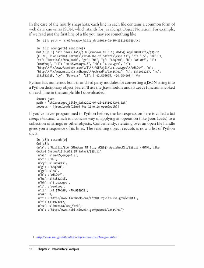
In the case of the hourly snapshots, each line in each file contains a common form ofweb data known as JSON, which stands for JavaScript Object Notation. For example,if we read just the first line of a file you may see something like
In [15]: path = 'ch02/usagov_bitly_data2012-03-16-1331923249.txt'
In [16]: open(path).readline()Out[16]: '{ "a": "Mozilla\\/5.0 (Windows NT 6.1; WOW64) AppleWebKit\\/535.11(KHTML, like Gecko) Chrome\\/17.0.963.78 Safari\\/535.11", "c": "US", "nk": 1,"tz": "America\\/New_York", "gr": "MA", "g": "A6qOVH", "h": "wfLQtf", "l":"orofrog", "al": "en-US,en;q=0.8", "hh": "1.usa.gov", "r":"http:\\/\\/www.facebook.com\\/l\\/7AQEFzjSi\\/1.usa.gov\\/wfLQtf", "u":"http:\\/\\/www.ncbi.nlm.nih.gov\\/pubmed\\/22415991", "t": 1331923247, "hc":1331822918, "cy": "Danvers", "ll": [ 42.576698, -70.954903 ] }\n'
Python has numerous built-in and 3rd party modules for converting a JSON string intoa Python dictionary object. Here I’ll use the json module and its loads function invokedon each line in the sample file I downloaded:
import jsonpath = 'ch02/usagov_bitly_data2012-03-16-1331923249.txt'records = [json.loads(line) for line in open(path)]
If you’ve never programmed in Python before, the last expression here is called a listcomprehension, which is a concise way of applying an operation (like json.loads) to acollection of strings or other objects. Conveniently, iterating over an open file handlegives you a sequence of its lines. The resulting object records is now a list of Pythondicts:
In [18]: records[0]Out[18]:{u'a': u'Mozilla/5.0 (Windows NT 6.1; WOW64) AppleWebKit/535.11 (KHTML, likeGecko) Chrome/17.0.963.78 Safari/535.11', u'al': u'en-US,en;q=0.8', u'c': u'US', u'cy': u'Danvers', u'g': u'A6qOVH', u'gr': u'MA', u'h': u'wfLQtf', u'hc': 1331822918, u'hh': u'1.usa.gov', u'l': u'orofrog', u'll': [42.576698, -70.954903], u'nk': 1, u'r': u'http://www.facebook.com/l/7AQEFzjSi/1.usa.gov/wfLQtf', u't': 1331923247, u'tz': u'America/New_York', u'u': u'http://www.ncbi.nlm.nih.gov/pubmed/22415991'}
1. http://www.usa.gov/About/developer-resources/1usagov.shtml
18 | Chapter 2: Introductory Examples
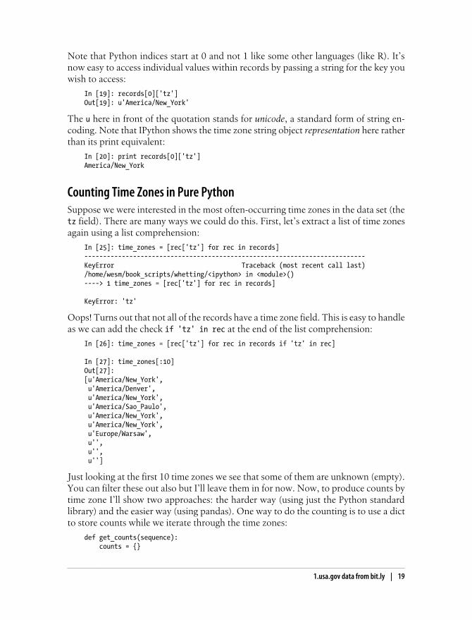
Note that Python indices start at 0 and not 1 like some other languages (like R). It’snow easy to access individual values within records by passing a string for the key youwish to access:
In [19]: records[0]['tz']Out[19]: u'America/New_York'
The u here in front of the quotation stands for unicode, a standard form of string en-coding. Note that IPython shows the time zone string object representation here ratherthan its print equivalent:
In [20]: print records[0]['tz']America/New_York
Counting Time Zones in Pure PythonSuppose we were interested in the most often-occurring time zones in the data set (thetz field). There are many ways we could do this. First, let’s extract a list of time zonesagain using a list comprehension:
In [25]: time_zones = [rec['tz'] for rec in records]---------------------------------------------------------------------------KeyError Traceback (most recent call last)/home/wesm/book_scripts/whetting/<ipython> in <module>()----> 1 time_zones = [rec['tz'] for rec in records]
KeyError: 'tz'
Oops! Turns out that not all of the records have a time zone field. This is easy to handleas we can add the check if 'tz' in rec at the end of the list comprehension:
In [26]: time_zones = [rec['tz'] for rec in records if 'tz' in rec]
In [27]: time_zones[:10]Out[27]:[u'America/New_York', u'America/Denver', u'America/New_York', u'America/Sao_Paulo', u'America/New_York', u'America/New_York', u'Europe/Warsaw', u'', u'', u'']
Just looking at the first 10 time zones we see that some of them are unknown (empty).You can filter these out also but I’ll leave them in for now. Now, to produce counts bytime zone I’ll show two approaches: the harder way (using just the Python standardlibrary) and the easier way (using pandas). One way to do the counting is to use a dictto store counts while we iterate through the time zones:
def get_counts(sequence): counts = {}
1.usa.gov data from bit.ly | 19

for x in sequence: if x in counts: counts[x] += 1 else: counts[x] = 1 return counts
If you know a bit more about the Python standard library, you might prefer to writethe same thing more briefly:
from collections import defaultdict
def get_counts2(sequence): counts = defaultdict(int) # values will initialize to 0 for x in sequence: counts[x] += 1 return counts
I put this logic in a function just to make it more reusable. To use it on the time zones,just pass the time_zones list:
In [31]: counts = get_counts(time_zones)
In [32]: counts['America/New_York']Out[32]: 1251
In [33]: len(time_zones)Out[33]: 3440
If we wanted the top 10 time zones and their counts, we have to do a little bit of dic-tionary acrobatics:
def top_counts(count_dict, n=10): value_key_pairs = [(count, tz) for tz, count in count_dict.items()] value_key_pairs.sort() return value_key_pairs[-n:]
We have then:
In [35]: top_counts(counts)Out[35]:[(33, u'America/Sao_Paulo'), (35, u'Europe/Madrid'), (36, u'Pacific/Honolulu'), (37, u'Asia/Tokyo'), (74, u'Europe/London'), (191, u'America/Denver'), (382, u'America/Los_Angeles'), (400, u'America/Chicago'), (521, u''), (1251, u'America/New_York')]
20 | Chapter 2: Introductory Examples
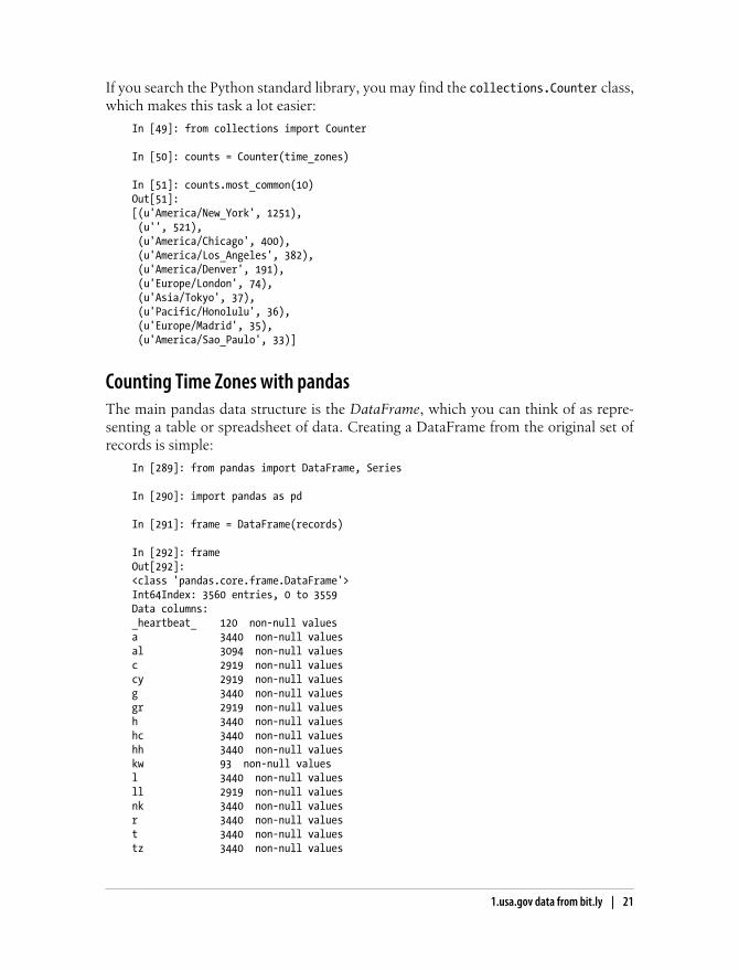
If you search the Python standard library, you may find the collections.Counter class,which makes this task a lot easier:
In [49]: from collections import Counter
In [50]: counts = Counter(time_zones)
In [51]: counts.most_common(10)Out[51]:[(u'America/New_York', 1251), (u'', 521), (u'America/Chicago', 400), (u'America/Los_Angeles', 382), (u'America/Denver', 191), (u'Europe/London', 74), (u'Asia/Tokyo', 37), (u'Pacific/Honolulu', 36), (u'Europe/Madrid', 35), (u'America/Sao_Paulo', 33)]
Counting Time Zones with pandasThe main pandas data structure is the DataFrame, which you can think of as repre-senting a table or spreadsheet of data. Creating a DataFrame from the original set ofrecords is simple:
In [289]: from pandas import DataFrame, Series
In [290]: import pandas as pd
In [291]: frame = DataFrame(records)
In [292]: frameOut[292]: <class 'pandas.core.frame.DataFrame'>Int64Index: 3560 entries, 0 to 3559Data columns:_heartbeat_ 120 non-null valuesa 3440 non-null valuesal 3094 non-null valuesc 2919 non-null valuescy 2919 non-null valuesg 3440 non-null valuesgr 2919 non-null valuesh 3440 non-null valueshc 3440 non-null valueshh 3440 non-null valueskw 93 non-null valuesl 3440 non-null valuesll 2919 non-null valuesnk 3440 non-null valuesr 3440 non-null valuest 3440 non-null valuestz 3440 non-null values
1.usa.gov data from bit.ly | 21

u 3440 non-null valuesdtypes: float64(4), object(14)
In [293]: frame['tz'][:10]Out[293]: 0 America/New_York1 America/Denver2 America/New_York3 America/Sao_Paulo4 America/New_York5 America/New_York6 Europe/Warsaw7 8 9 Name: tz
The output shown for the frame is the summary view, shown for large DataFrame ob-jects. The Series object returned by frame['tz'] has a method value_counts that givesus what we’re looking for:
In [294]: tz_counts = frame['tz'].value_counts()
In [295]: tz_counts[:10]Out[295]: America/New_York 1251 521America/Chicago 400America/Los_Angeles 382America/Denver 191Europe/London 74Asia/Tokyo 37Pacific/Honolulu 36Europe/Madrid 35America/Sao_Paulo 33
Then, we might want to make a plot of this data using plotting library, matplotlib. Youcan do a bit of munging to fill in a substitute value for unknown and missing time zonedata in the records. The fillna function can replace missing (NA) values and unknown(empty strings) values can be replaced by boolean array indexing:
In [296]: clean_tz = frame['tz'].fillna('Missing')
In [297]: clean_tz[clean_tz == ''] = 'Unknown'
In [298]: tz_counts = clean_tz.value_counts()
In [299]: tz_counts[:10]Out[299]: America/New_York 1251Unknown 521America/Chicago 400America/Los_Angeles 382America/Denver 191Missing 120
22 | Chapter 2: Introductory Examples

Europe/London 74Asia/Tokyo 37Pacific/Honolulu 36Europe/Madrid 35
Making a horizontal bar plot can be accomplished using the plot method on thecounts objects:
In [301]: tz_counts[:10].plot(kind='barh', rot=0)
See Figure 2-1 for the resulting figure. We’ll explore more tools for working with thiskind of data. For example, the a field contains information about the browser, device,or application used to perform the URL shortening:
In [302]: frame['a'][1]Out[302]: u'GoogleMaps/RochesterNY'
In [303]: frame['a'][50]Out[303]: u'Mozilla/5.0 (Windows NT 5.1; rv:10.0.2) Gecko/20100101 Firefox/10.0.2'
In [304]: frame['a'][51]Out[304]: u'Mozilla/5.0 (Linux; U; Android 2.2.2; en-us; LG-P925/V10e Build/FRG83G) AppleWebKit/533.1 (KHTML, like Gecko) Version/4.0 Mobile Safari/533.1'
Figure 2-1. Top time zones in the 1.usa.gov sample data
Parsing all of the interesting information in these “agent” strings may seem like adaunting task. Luckily, once you have mastered Python’s built-in string functions andregular expression capabilities, it is really not so bad. For example, we could split offthe first token in the string (corresponding roughly to the browser capability) and makeanother summary of the user behavior:
In [305]: results = Series([x.split()[0] for x in frame.a.dropna()])
In [306]: results[:5]Out[306]: 0 Mozilla/5.01 GoogleMaps/RochesterNY2 Mozilla/4.03 Mozilla/5.04 Mozilla/5.0
1.usa.gov data from bit.ly | 23
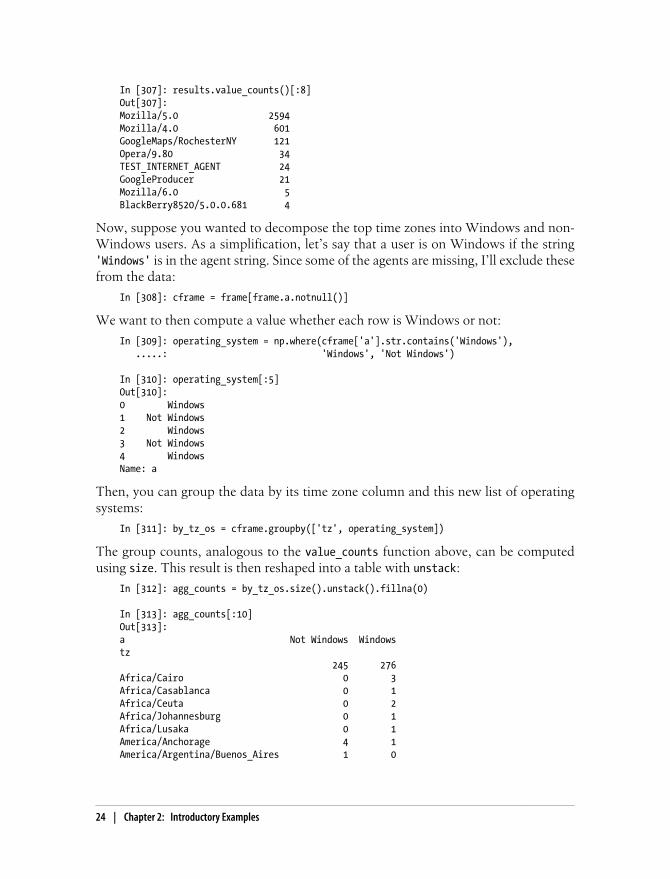
In [307]: results.value_counts()[:8]Out[307]: Mozilla/5.0 2594Mozilla/4.0 601GoogleMaps/RochesterNY 121Opera/9.80 34TEST_INTERNET_AGENT 24GoogleProducer 21Mozilla/6.0 5BlackBerry8520/5.0.0.681 4
Now, suppose you wanted to decompose the top time zones into Windows and non-Windows users. As a simplification, let’s say that a user is on Windows if the string'Windows' is in the agent string. Since some of the agents are missing, I’ll exclude thesefrom the data:
In [308]: cframe = frame[frame.a.notnull()]
We want to then compute a value whether each row is Windows or not:
In [309]: operating_system = np.where(cframe['a'].str.contains('Windows'), .....: 'Windows', 'Not Windows')
In [310]: operating_system[:5]Out[310]: 0 Windows1 Not Windows2 Windows3 Not Windows4 WindowsName: a
Then, you can group the data by its time zone column and this new list of operatingsystems:
In [311]: by_tz_os = cframe.groupby(['tz', operating_system])
The group counts, analogous to the value_counts function above, can be computedusing size. This result is then reshaped into a table with unstack:
In [312]: agg_counts = by_tz_os.size().unstack().fillna(0)
In [313]: agg_counts[:10]Out[313]: a Not Windows Windowstz 245 276Africa/Cairo 0 3Africa/Casablanca 0 1Africa/Ceuta 0 2Africa/Johannesburg 0 1Africa/Lusaka 0 1America/Anchorage 4 1America/Argentina/Buenos_Aires 1 0
24 | Chapter 2: Introductory Examples
America/Argentina/Cordoba 0 1America/Argentina/Mendoza 0 1
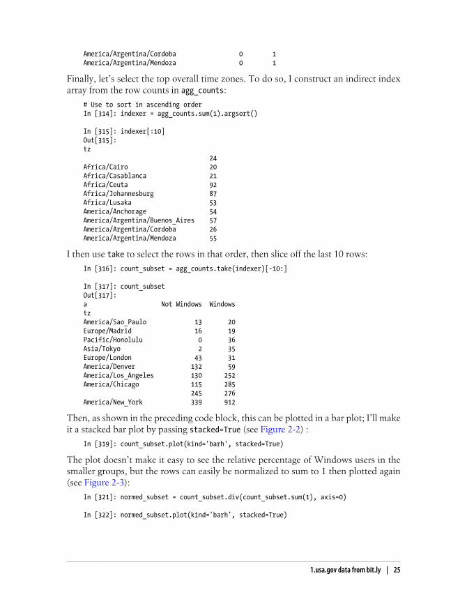
Finally, let’s select the top overall time zones. To do so, I construct an indirect indexarray from the row counts in agg_counts:
# Use to sort in ascending orderIn [314]: indexer = agg_counts.sum(1).argsort()
In [315]: indexer[:10]Out[315]: tz 24Africa/Cairo 20Africa/Casablanca 21Africa/Ceuta 92Africa/Johannesburg 87Africa/Lusaka 53America/Anchorage 54America/Argentina/Buenos_Aires 57America/Argentina/Cordoba 26America/Argentina/Mendoza 55
I then use take to select the rows in that order, then slice off the last 10 rows:
In [316]: count_subset = agg_counts.take(indexer)[-10:]
In [317]: count_subsetOut[317]: a Not Windows Windowstz America/Sao_Paulo 13 20Europe/Madrid 16 19Pacific/Honolulu 0 36Asia/Tokyo 2 35Europe/London 43 31America/Denver 132 59America/Los_Angeles 130 252America/Chicago 115 285 245 276America/New_York 339 912
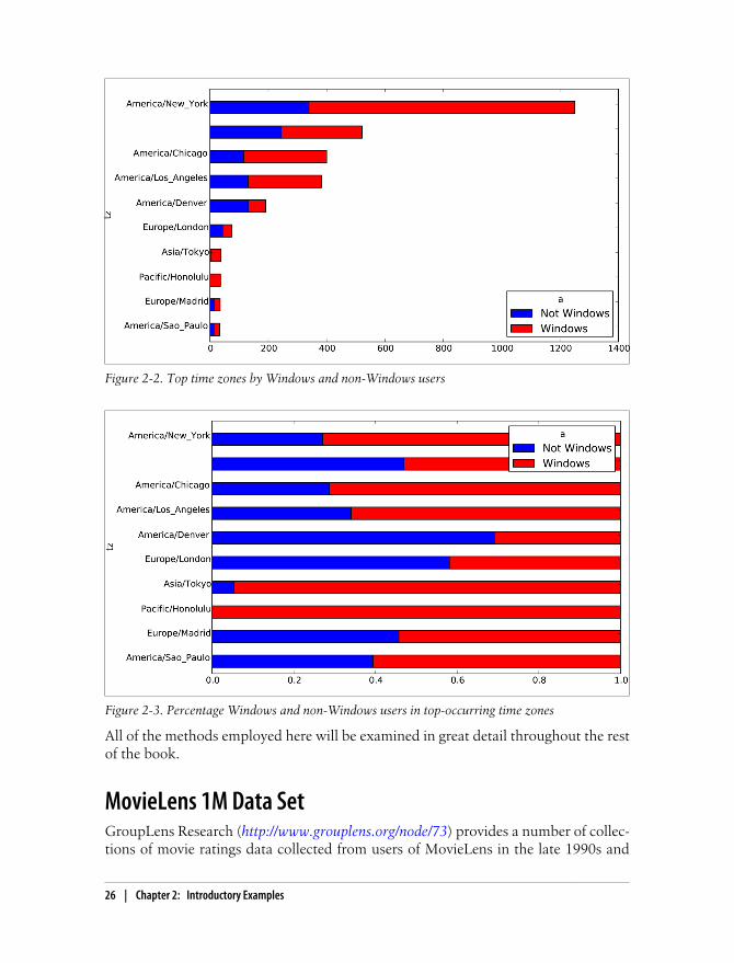
Then, as shown in the preceding code block, this can be plotted in a bar plot; I’ll makeit a stacked bar plot by passing stacked=True (see Figure 2-2) :
In [319]: count_subset.plot(kind='barh', stacked=True)
The plot doesn’t make it easy to see the relative percentage of Windows users in thesmaller groups, but the rows can easily be normalized to sum to 1 then plotted again(see Figure 2-3):
In [321]: normed_subset = count_subset.div(count_subset.sum(1), axis=0)
In [322]: normed_subset.plot(kind='barh', stacked=True)
1.usa.gov data from bit.ly | 25
All of the methods employed here will be examined in great detail throughout the restof the book.
MovieLens 1M Data SetGroupLens Research (http://www.grouplens.org/node/73) provides a number of collec-tions of movie ratings data collected from users of MovieLens in the late 1990s and
Figure 2-2. Top time zones by Windows and non-Windows users
Figure 2-3. Percentage Windows and non-Windows users in top-occurring time zones
26 | Chapter 2: Introductory Examples
early 2000s. The data provide movie ratings, movie metadata (genres and year), anddemographic data about the users (age, zip code, gender, and occupation). Such datais often of interest in the development of recommendation systems based on machinelearning algorithms. While I will not be exploring machine learning techniques in greatdetail in this book, I will show you how to slice and dice data sets like these into theexact form you need.
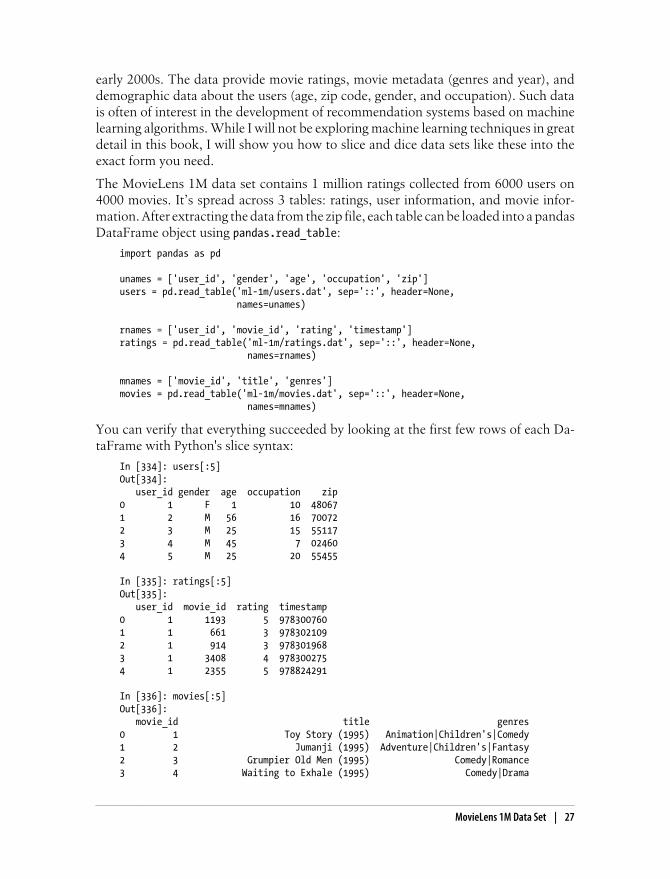
The MovieLens 1M data set contains 1 million ratings collected from 6000 users on4000 movies. It’s spread across 3 tables: ratings, user information, and movie infor-mation. After extracting the data from the zip file, each table can be loaded into a pandasDataFrame object using pandas.read_table:
import pandas as pd
unames = ['user_id', 'gender', 'age', 'occupation', 'zip']users = pd.read_table('ml-1m/users.dat', sep='::', header=None, names=unames)
rnames = ['user_id', 'movie_id', 'rating', 'timestamp']ratings = pd.read_table('ml-1m/ratings.dat', sep='::', header=None, names=rnames)
mnames = ['movie_id', 'title', 'genres']movies = pd.read_table('ml-1m/movies.dat', sep='::', header=None, names=mnames)
You can verify that everything succeeded by looking at the first few rows of each Da-taFrame with Python's slice syntax:
In [334]: users[:5]Out[334]: user_id gender age occupation zip0 1 F 1 10 480671 2 M 56 16 700722 3 M 25 15 551173 4 M 45 7 024604 5 M 25 20 55455
In [335]: ratings[:5]Out[335]: user_id movie_id rating timestamp0 1 1193 5 9783007601 1 661 3 9783021092 1 914 3 9783019683 1 3408 4 9783002754 1 2355 5 978824291
In [336]: movies[:5]Out[336]: movie_id title genres0 1 Toy Story (1995) Animation|Children's|Comedy1 2 Jumanji (1995) Adventure|Children's|Fantasy2 3 Grumpier Old Men (1995) Comedy|Romance3 4 Waiting to Exhale (1995) Comedy|Drama
MovieLens 1M Data Set | 27
4 5 Father of the Bride Part II (1995) Comedy
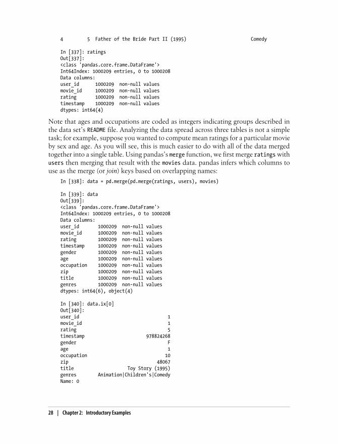
In [337]: ratingsOut[337]: <class 'pandas.core.frame.DataFrame'>Int64Index: 1000209 entries, 0 to 1000208Data columns:user_id 1000209 non-null valuesmovie_id 1000209 non-null valuesrating 1000209 non-null valuestimestamp 1000209 non-null valuesdtypes: int64(4)
Note that ages and occupations are coded as integers indicating groups described inthe data set’s README file. Analyzing the data spread across three tables is not a simpletask; for example, suppose you wanted to compute mean ratings for a particular movieby sex and age. As you will see, this is much easier to do with all of the data mergedtogether into a single table. Using pandas’s merge function, we first merge ratings withusers then merging that result with the movies data. pandas infers which columns touse as the merge (or join) keys based on overlapping names:
In [338]: data = pd.merge(pd.merge(ratings, users), movies)
In [339]: dataOut[339]: <class 'pandas.core.frame.DataFrame'>Int64Index: 1000209 entries, 0 to 1000208Data columns:user_id 1000209 non-null valuesmovie_id 1000209 non-null valuesrating 1000209 non-null valuestimestamp 1000209 non-null valuesgender 1000209 non-null valuesage 1000209 non-null valuesoccupation 1000209 non-null valueszip 1000209 non-null valuestitle 1000209 non-null valuesgenres 1000209 non-null valuesdtypes: int64(6), object(4)
In [340]: data.ix[0]Out[340]: user_id 1movie_id 1rating 5timestamp 978824268gender Fage 1occupation 10zip 48067title Toy Story (1995)genres Animation|Children's|ComedyName: 0
28 | Chapter 2: Introductory Examples
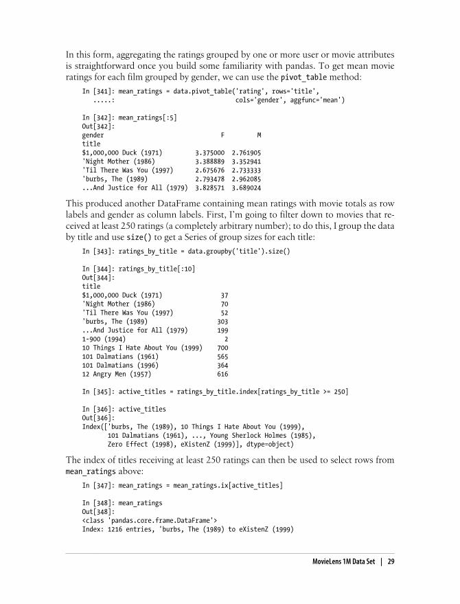
In this form, aggregating the ratings grouped by one or more user or movie attributesis straightforward once you build some familiarity with pandas. To get mean movieratings for each film grouped by gender, we can use the pivot_table method:
In [341]: mean_ratings = data.pivot_table('rating', rows='title', .....: cols='gender', aggfunc='mean')
In [342]: mean_ratings[:5]Out[342]: gender F Mtitle $1,000,000 Duck (1971) 3.375000 2.761905'Night Mother (1986) 3.388889 3.352941'Til There Was You (1997) 2.675676 2.733333'burbs, The (1989) 2.793478 2.962085...And Justice for All (1979) 3.828571 3.689024
This produced another DataFrame containing mean ratings with movie totals as rowlabels and gender as column labels. First, I’m going to filter down to movies that re-ceived at least 250 ratings (a completely arbitrary number); to do this, I group the databy title and use size() to get a Series of group sizes for each title:
In [343]: ratings_by_title = data.groupby('title').size()
In [344]: ratings_by_title[:10]Out[344]: title$1,000,000 Duck (1971) 37'Night Mother (1986) 70'Til There Was You (1997) 52'burbs, The (1989) 303...And Justice for All (1979) 1991-900 (1994) 210 Things I Hate About You (1999) 700101 Dalmatians (1961) 565101 Dalmatians (1996) 36412 Angry Men (1957) 616
In [345]: active_titles = ratings_by_title.index[ratings_by_title >= 250]
In [346]: active_titlesOut[346]: Index(['burbs, The (1989), 10 Things I Hate About You (1999), 101 Dalmatians (1961), ..., Young Sherlock Holmes (1985), Zero Effect (1998), eXistenZ (1999)], dtype=object)
The index of titles receiving at least 250 ratings can then be used to select rows frommean_ratings above:
In [347]: mean_ratings = mean_ratings.ix[active_titles]
In [348]: mean_ratingsOut[348]: <class 'pandas.core.frame.DataFrame'>Index: 1216 entries, 'burbs, The (1989) to eXistenZ (1999)
MovieLens 1M Data Set | 29

Data columns:F 1216 non-null valuesM 1216 non-null valuesdtypes: float64(2)
To see the top films among female viewers, we can sort by the F column in descendingorder:
In [350]: top_female_ratings = mean_ratings.sort_index(by='F', ascending=False)
In [351]: top_female_ratings[:10]Out[351]: gender F MClose Shave, A (1995) 4.644444 4.473795Wrong Trousers, The (1993) 4.588235 4.478261Sunset Blvd. (a.k.a. Sunset Boulevard) (1950) 4.572650 4.464589Wallace & Gromit: The Best of Aardman Animation (1996) 4.563107 4.385075Schindler's List (1993) 4.562602 4.491415Shawshank Redemption, The (1994) 4.539075 4.560625Grand Day Out, A (1992) 4.537879 4.293255To Kill a Mockingbird (1962) 4.536667 4.372611Creature Comforts (1990) 4.513889 4.272277Usual Suspects, The (1995) 4.513317 4.518248
Measuring rating disagreementSuppose you wanted to find the movies that are most divisive between male and femaleviewers. One way is to add a column to mean_ratings containing the difference inmeans, then sort by that:
In [352]: mean_ratings['diff'] = mean_ratings['M'] - mean_ratings['F']
Sorting by 'diff' gives us the movies with the greatest rating difference and which werepreferred by women:
In [353]: sorted_by_diff = mean_ratings.sort_index(by='diff')
In [354]: sorted_by_diff[:15]Out[354]: gender F M diffDirty Dancing (1987) 3.790378 2.959596 -0.830782Jumpin' Jack Flash (1986) 3.254717 2.578358 -0.676359Grease (1978) 3.975265 3.367041 -0.608224Little Women (1994) 3.870588 3.321739 -0.548849Steel Magnolias (1989) 3.901734 3.365957 -0.535777Anastasia (1997) 3.800000 3.281609 -0.518391Rocky Horror Picture Show, The (1975) 3.673016 3.160131 -0.512885Color Purple, The (1985) 4.158192 3.659341 -0.498851Age of Innocence, The (1993) 3.827068 3.339506 -0.487561Free Willy (1993) 2.921348 2.438776 -0.482573French Kiss (1995) 3.535714 3.056962 -0.478752Little Shop of Horrors, The (1960) 3.650000 3.179688 -0.470312Guys and Dolls (1955) 4.051724 3.583333 -0.468391Mary Poppins (1964) 4.197740 3.730594 -0.467147Patch Adams (1998) 3.473282 3.008746 -0.464536
30 | Chapter 2: Introductory Examples

Reversing the order of the rows and again slicing off the top 15 rows, we get the moviespreferred by men that women didn’t rate as highly:
# Reverse order of rows, take first 15 rowsIn [355]: sorted_by_diff[::-1][:15]Out[355]: gender F M diffGood, The Bad and The Ugly, The (1966) 3.494949 4.221300 0.726351Kentucky Fried Movie, The (1977) 2.878788 3.555147 0.676359Dumb & Dumber (1994) 2.697987 3.336595 0.638608Longest Day, The (1962) 3.411765 4.031447 0.619682Cable Guy, The (1996) 2.250000 2.863787 0.613787Evil Dead II (Dead By Dawn) (1987) 3.297297 3.909283 0.611985Hidden, The (1987) 3.137931 3.745098 0.607167Rocky III (1982) 2.361702 2.943503 0.581801Caddyshack (1980) 3.396135 3.969737 0.573602For a Few Dollars More (1965) 3.409091 3.953795 0.544704Porky's (1981) 2.296875 2.836364 0.539489Animal House (1978) 3.628906 4.167192 0.538286Exorcist, The (1973) 3.537634 4.067239 0.529605Fright Night (1985) 2.973684 3.500000 0.526316Barb Wire (1996) 1.585366 2.100386 0.515020
Suppose instead you wanted the movies that elicited the most disagreement amongviewers, independent of gender. Disagreement can be measured by the variance orstandard deviation of the ratings:
# Standard deviation of rating grouped by titleIn [356]: rating_std_by_title = data.groupby('title')['rating'].std()
# Filter down to active_titlesIn [357]: rating_std_by_title = rating_std_by_title.ix[active_titles]
# Order Series by value in descending orderIn [358]: rating_std_by_title.order(ascending=False)[:10]Out[358]: titleDumb & Dumber (1994) 1.321333Blair Witch Project, The (1999) 1.316368Natural Born Killers (1994) 1.307198Tank Girl (1995) 1.277695Rocky Horror Picture Show, The (1975) 1.260177Eyes Wide Shut (1999) 1.259624Evita (1996) 1.253631Billy Madison (1995) 1.249970Fear and Loathing in Las Vegas (1998) 1.246408Bicentennial Man (1999) 1.245533Name: rating
You may have noticed that movie genres are given as a pipe-separated (|) string. If youwanted to do some analysis by genre, more work would be required to transform thegenre information into a more usable form. I will revisit this data later in the book toillustrate such a transformation.
MovieLens 1M Data Set | 31
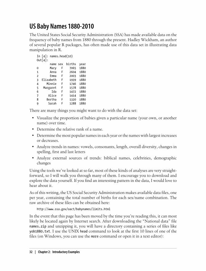
US Baby Names 1880-2010The United States Social Security Administration (SSA) has made available data on thefrequency of baby names from 1880 through the present. Hadley Wickham, an authorof several popular R packages, has often made use of this data set in illustrating datamanipulation in R.
In [4]: names.head(10)Out[4]: name sex births year0 Mary F 7065 18801 Anna F 2604 18802 Emma F 2003 18803 Elizabeth F 1939 18804 Minnie F 1746 18805 Margaret F 1578 18806 Ida F 1472 18807 Alice F 1414 18808 Bertha F 1320 18809 Sarah F 1288 1880
There are many things you might want to do with the data set:
• Visualize the proportion of babies given a particular name (your own, or anothername) over time.
• Determine the relative rank of a name.
• Determine the most popular names in each year or the names with largest increasesor decreases.
• Analyze trends in names: vowels, consonants, length, overall diversity, changes inspelling, first and last letters
• Analyze external sources of trends: biblical names, celebrities, demographicchanges
Using the tools we’ve looked at so far, most of these kinds of analyses are very straight-forward, so I will walk you through many of them. I encourage you to download andexplore the data yourself. If you find an interesting pattern in the data, I would love tohear about it.
As of this writing, the US Social Security Administration makes available data files, oneper year, containing the total number of births for each sex/name combination. Theraw archive of these files can be obtained here:
http://www.ssa.gov/oact/babynames/limits.html
In the event that this page has been moved by the time you’re reading this, it can mostlikely be located again by Internet search. After downloading the “National data” filenames.zip and unzipping it, you will have a directory containing a series of files likeyob1880.txt. I use the UNIX head command to look at the first 10 lines of one of thefiles (on Windows, you can use the more command or open it in a text editor):
32 | Chapter 2: Introductory Examples

In [367]: !head -n 10 names/yob1880.txtMary,F,7065Anna,F,2604Emma,F,2003Elizabeth,F,1939Minnie,F,1746Margaret,F,1578Ida,F,1472Alice,F,1414Bertha,F,1320Sarah,F,1288
As this is a nicely comma-separated form, it can be loaded into a DataFrame withpandas.read_csv:
In [368]: import pandas as pd
In [369]: names1880 = pd.read_csv('names/yob1880.txt', names=['name', 'sex', 'births'])
In [370]: names1880Out[370]: <class 'pandas.core.frame.DataFrame'>Int64Index: 2000 entries, 0 to 1999Data columns:name 2000 non-null valuessex 2000 non-null valuesbirths 2000 non-null valuesdtypes: int64(1), object(2)
These files only contain names with at least 5 occurrences in each year, so for simplic-ity’s sake we can use the sum of the births column by sex as the total number of birthsin that year:
In [371]: names1880.groupby('sex').births.sum()Out[371]: sexF 90993M 110493Name: births
Since the data set is split into files by year, one of the first things to do is to assembleall of the data into a single DataFrame and further to add a year field. This is easy todo using pandas.concat:
# 2010 is the last available year right nowyears = range(1880, 2011)
pieces = []columns = ['name', 'sex', 'births']
for year in years: path = 'names/yob%d.txt' % year frame = pd.read_csv(path, names=columns)
frame['year'] = year pieces.append(frame)
US Baby Names 1880-2010 | 33
# Concatenate everything into a single DataFramenames = pd.concat(pieces, ignore_index=True)
There are a couple things to note here. First, remember that concat glues the DataFrameobjects together row-wise by default. Secondly, you have to pass ignore_index=Truebecause we’re not interested in preserving the original row numbers returned fromread_csv. So we now have a very large DataFrame containing all of the names data:
Now the names DataFrame looks like:
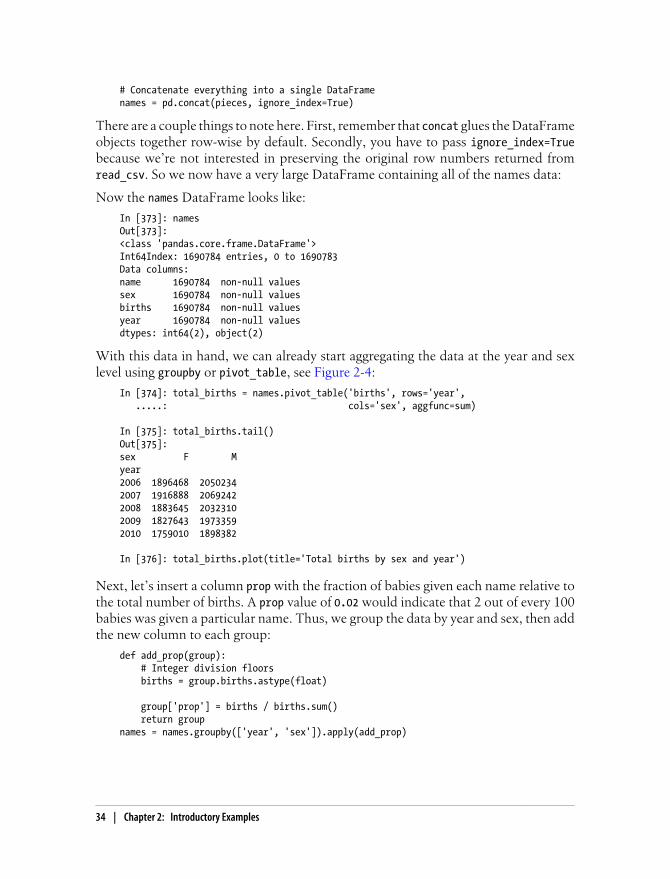
In [373]: namesOut[373]: <class 'pandas.core.frame.DataFrame'>Int64Index: 1690784 entries, 0 to 1690783Data columns:name 1690784 non-null valuessex 1690784 non-null valuesbirths 1690784 non-null valuesyear 1690784 non-null valuesdtypes: int64(2), object(2)
With this data in hand, we can already start aggregating the data at the year and sexlevel using groupby or pivot_table, see Figure 2-4:
In [374]: total_births = names.pivot_table('births', rows='year', .....: cols='sex', aggfunc=sum)
In [375]: total_births.tail()Out[375]: sex F Myear 2006 1896468 20502342007 1916888 20692422008 1883645 20323102009 1827643 19733592010 1759010 1898382
In [376]: total_births.plot(title='Total births by sex and year')
Next, let’s insert a column prop with the fraction of babies given each name relative tothe total number of births. A prop value of 0.02 would indicate that 2 out of every 100babies was given a particular name. Thus, we group the data by year and sex, then addthe new column to each group:
def add_prop(group): # Integer division floors births = group.births.astype(float)
group['prop'] = births / births.sum() return groupnames = names.groupby(['year', 'sex']).apply(add_prop)
34 | Chapter 2: Introductory Examples
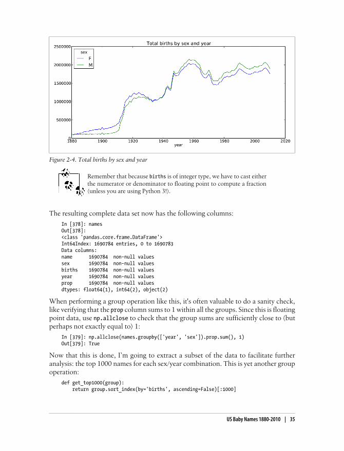
Remember that because births is of integer type, we have to cast eitherthe numerator or denominator to floating point to compute a fraction(unless you are using Python 3!).
The resulting complete data set now has the following columns:
In [378]: namesOut[378]: <class 'pandas.core.frame.DataFrame'>Int64Index: 1690784 entries, 0 to 1690783Data columns:name 1690784 non-null valuessex 1690784 non-null valuesbirths 1690784 non-null valuesyear 1690784 non-null valuesprop 1690784 non-null valuesdtypes: float64(1), int64(2), object(2)
When performing a group operation like this, it's often valuable to do a sanity check,like verifying that the prop column sums to 1 within all the groups. Since this is floatingpoint data, use np.allclose to check that the group sums are sufficiently close to (butperhaps not exactly equal to) 1:
In [379]: np.allclose(names.groupby(['year', 'sex']).prop.sum(), 1)Out[379]: True
Now that this is done, I’m going to extract a subset of the data to facilitate furtheranalysis: the top 1000 names for each sex/year combination. This is yet another groupoperation:
def get_top1000(group): return group.sort_index(by='births', ascending=False)[:1000]
Figure 2-4. Total births by sex and year
US Baby Names 1880-2010 | 35

grouped = names.groupby(['year', 'sex'])top1000 = grouped.apply(get_top1000)
If you prefer a do-it-yourself approach, you could also do:
pieces = []for year, group in names.groupby(['year', 'sex']): pieces.append(group.sort_index(by='births', ascending=False)[:1000])top1000 = pd.concat(pieces, ignore_index=True)
The resulting data set is now quite a bit smaller:
In [382]: top1000Out[382]: <class 'pandas.core.frame.DataFrame'>Int64Index: 261877 entries, 0 to 261876Data columns:name 261877 non-null valuessex 261877 non-null valuesbirths 261877 non-null valuesyear 261877 non-null valuesprop 261877 non-null valuesdtypes: float64(1), int64(2), object(2)
We’ll use this Top 1,000 data set in the following investigations into the data.
Analyzing Naming TrendsWith the full data set and Top 1,000 data set in hand, we can start analyzing variousnaming trends of interest. Splitting the Top 1,000 names into the boy and girl portionsis easy to do first:
In [383]: boys = top1000[top1000.sex == 'M']
In [384]: girls = top1000[top1000.sex == 'F']
Simple time series, like the number of Johns or Marys for each year can be plotted butrequire a bit of munging to be a bit more useful. Let’s form a pivot table of the totalnumber of births by year and name:
In [385]: total_births = top1000.pivot_table('births', rows='year', cols='name', .....: aggfunc=sum)
Now, this can be plotted for a handful of names using DataFrame’s plot method:
In [386]: total_birthsOut[386]: <class 'pandas.core.frame.DataFrame'>Int64Index: 131 entries, 1880 to 2010Columns: 6865 entries, Aaden to Zuridtypes: float64(6865)
In [387]: subset = total_births[['John', 'Harry', 'Mary', 'Marilyn']]
In [388]: subset.plot(subplots=True, figsize=(12, 10), grid=False, .....: title="Number of births per year")
36 | Chapter 2: Introductory Examples
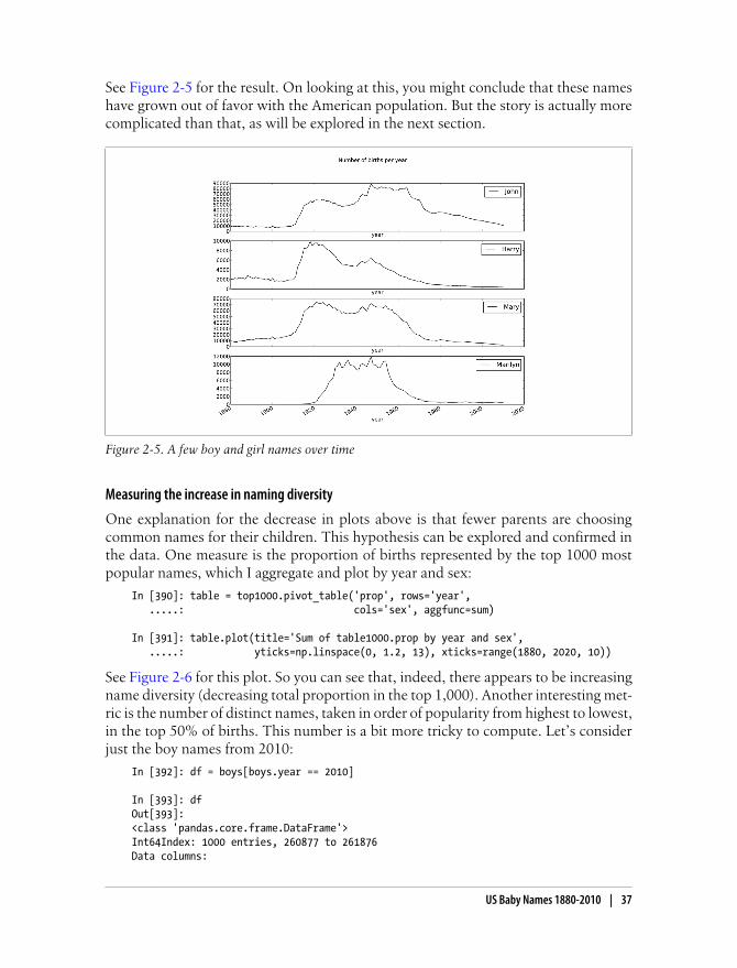
See Figure 2-5 for the result. On looking at this, you might conclude that these nameshave grown out of favor with the American population. But the story is actually morecomplicated than that, as will be explored in the next section.
Figure 2-5. A few boy and girl names over time
Measuring the increase in naming diversity
One explanation for the decrease in plots above is that fewer parents are choosingcommon names for their children. This hypothesis can be explored and confirmed inthe data. One measure is the proportion of births represented by the top 1000 mostpopular names, which I aggregate and plot by year and sex:
In [390]: table = top1000.pivot_table('prop', rows='year', .....: cols='sex', aggfunc=sum)
In [391]: table.plot(title='Sum of table1000.prop by year and sex', .....: yticks=np.linspace(0, 1.2, 13), xticks=range(1880, 2020, 10))
See Figure 2-6 for this plot. So you can see that, indeed, there appears to be increasingname diversity (decreasing total proportion in the top 1,000). Another interesting met-ric is the number of distinct names, taken in order of popularity from highest to lowest,in the top 50% of births. This number is a bit more tricky to compute. Let’s considerjust the boy names from 2010:
In [392]: df = boys[boys.year == 2010]
In [393]: dfOut[393]: <class 'pandas.core.frame.DataFrame'>Int64Index: 1000 entries, 260877 to 261876Data columns:
US Baby Names 1880-2010 | 37
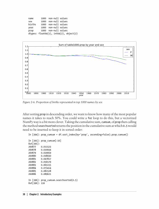
name 1000 non-null valuessex 1000 non-null valuesbirths 1000 non-null valuesyear 1000 non-null valuesprop 1000 non-null valuesdtypes: float64(1), int64(2), object(2)
Figure 2-6. Proportion of births represented in top 1000 names by sex
After sorting prop in descending order, we want to know how many of the most popularnames it takes to reach 50%. You could write a for loop to do this, but a vectorizedNumPy way is a bit more clever. Taking the cumulative sum, cumsum, of prop then callingthe method searchsorted returns the position in the cumulative sum at which 0.5 wouldneed to be inserted to keep it in sorted order:
In [394]: prop_cumsum = df.sort_index(by='prop', ascending=False).prop.cumsum()
In [395]: prop_cumsum[:10]Out[395]: 260877 0.011523260878 0.020934260879 0.029959260880 0.038930260881 0.047817260882 0.056579260883 0.065155260884 0.073414260885 0.081528260886 0.089621
In [396]: prop_cumsum.searchsorted(0.5)Out[396]: 116
38 | Chapter 2: Introductory Examples
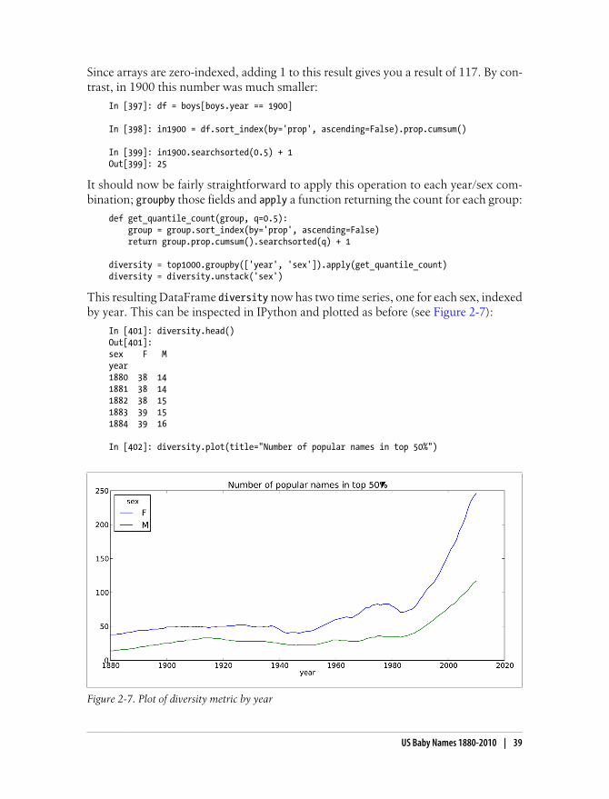
Since arrays are zero-indexed, adding 1 to this result gives you a result of 117. By con-trast, in 1900 this number was much smaller:
In [397]: df = boys[boys.year == 1900]
In [398]: in1900 = df.sort_index(by='prop', ascending=False).prop.cumsum()
In [399]: in1900.searchsorted(0.5) + 1Out[399]: 25
It should now be fairly straightforward to apply this operation to each year/sex com-bination; groupby those fields and apply a function returning the count for each group:
def get_quantile_count(group, q=0.5): group = group.sort_index(by='prop', ascending=False) return group.prop.cumsum().searchsorted(q) + 1
diversity = top1000.groupby(['year', 'sex']).apply(get_quantile_count)diversity = diversity.unstack('sex')
This resulting DataFrame diversity now has two time series, one for each sex, indexedby year. This can be inspected in IPython and plotted as before (see Figure 2-7):
In [401]: diversity.head()Out[401]: sex F Myear 1880 38 141881 38 141882 38 151883 39 151884 39 16
In [402]: diversity.plot(title="Number of popular names in top 50%")
Figure 2-7. Plot of diversity metric by year
US Baby Names 1880-2010 | 39
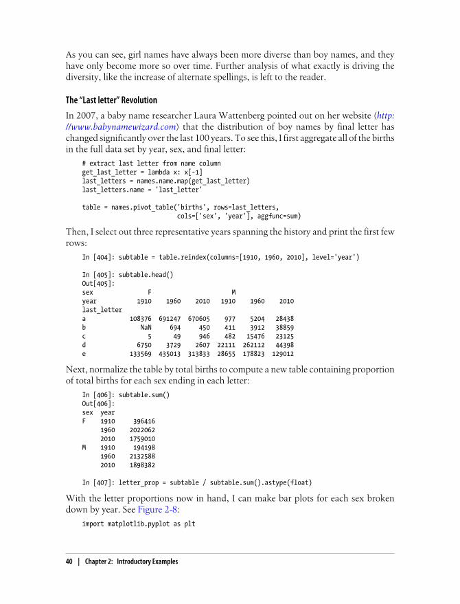
As you can see, girl names have always been more diverse than boy names, and theyhave only become more so over time. Further analysis of what exactly is driving thediversity, like the increase of alternate spellings, is left to the reader.
The “Last letter” Revolution
In 2007, a baby name researcher Laura Wattenberg pointed out on her website (http://www.babynamewizard.com) that the distribution of boy names by final letter haschanged significantly over the last 100 years. To see this, I first aggregate all of the birthsin the full data set by year, sex, and final letter:
# extract last letter from name columnget_last_letter = lambda x: x[-1]last_letters = names.name.map(get_last_letter)last_letters.name = 'last_letter'
table = names.pivot_table('births', rows=last_letters, cols=['sex', 'year'], aggfunc=sum)
Then, I select out three representative years spanning the history and print the first fewrows:
In [404]: subtable = table.reindex(columns=[1910, 1960, 2010], level='year')
In [405]: subtable.head()Out[405]: sex F M year 1910 1960 2010 1910 1960 2010last_letter a 108376 691247 670605 977 5204 28438b NaN 694 450 411 3912 38859c 5 49 946 482 15476 23125d 6750 3729 2607 22111 262112 44398e 133569 435013 313833 28655 178823 129012
Next, normalize the table by total births to compute a new table containing proportionof total births for each sex ending in each letter:
In [406]: subtable.sum()Out[406]: sex yearF 1910 396416 1960 2022062 2010 1759010M 1910 194198 1960 2132588 2010 1898382
In [407]: letter_prop = subtable / subtable.sum().astype(float)
With the letter proportions now in hand, I can make bar plots for each sex brokendown by year. See Figure 2-8:
import matplotlib.pyplot as plt
40 | Chapter 2: Introductory Examples
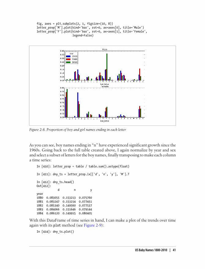
fig, axes = plt.subplots(2, 1, figsize=(10, 8))letter_prop['M'].plot(kind='bar', rot=0, ax=axes[0], title='Male')letter_prop['F'].plot(kind='bar', rot=0, ax=axes[1], title='Female', legend=False)
Figure 2-8. Proportion of boy and girl names ending in each letter
As you can see, boy names ending in “n” have experienced significant growth since the1960s. Going back to the full table created above, I again normalize by year and sexand select a subset of letters for the boy names, finally transposing to make each columna time series:
In [410]: letter_prop = table / table.sum().astype(float)
In [411]: dny_ts = letter_prop.ix[['d', 'n', 'y'], 'M'].T
In [412]: dny_ts.head()Out[412]: d n yyear 1880 0.083055 0.153213 0.0757601881 0.083247 0.153214 0.0774511882 0.085340 0.149560 0.0775371883 0.084066 0.151646 0.0791441884 0.086120 0.149915 0.080405
With this DataFrame of time series in hand, I can make a plot of the trends over timeagain with its plot method (see Figure 2-9):
In [414]: dny_ts.plot()
US Baby Names 1880-2010 | 41

Figure 2-9. Proportion of boys born with names ending in d/n/y over time
Boy names that became girl names (and vice versa)
Another fun trend is looking at boy names that were more popular with one sex earlierin the sample but have “changed sexes” in the present. One example is the name Lesleyor Leslie. Going back to the top1000 dataset, I compute a list of names occurring in thedataset starting with 'lesl':
In [415]: all_names = top1000.name.unique()
In [416]: mask = np.array(['lesl' in x.lower() for x in all_names])
In [417]: lesley_like = all_names[mask]
In [418]: lesley_likeOut[418]: array([Leslie, Lesley, Leslee, Lesli, Lesly], dtype=object)
From there, we can filter down to just those names and sum births grouped by nameto see the relative frequencies:
In [419]: filtered = top1000[top1000.name.isin(lesley_like)]
In [420]: filtered.groupby('name').births.sum()Out[420]: nameLeslee 1082Lesley 35022Lesli 929Leslie 370429Lesly 10067Name: births
Next, let’s aggregate by sex and year and normalize within year:
42 | Chapter 2: Introductory Examples

In [421]: table = filtered.pivot_table('births', rows='year', .....: cols='sex', aggfunc='sum')
In [422]: table = table.div(table.sum(1), axis=0)
In [423]: table.tail()Out[423]: sex F Myear 2006 1 NaN2007 1 NaN2008 1 NaN2009 1 NaN2010 1 NaN
Lastly, it’s now easy to make a plot of the breakdown by sex over time (Figure 2-10):
In [425]: table.plot(style={'M': 'k-', 'F': 'k--'})
Figure 2-10. Proportion of male/female Lesley-like names over time
Conclusions and The Path AheadThe examples in this chapter are rather simple, but they’re here to give you a bit of aflavor of what sorts of things you can expect in the upcoming chapters. The focus ofthis book is on tools as opposed to presenting more sophisticated analytical methods.Mastering the techniques in this book will enable you to implement your own analyses(assuming you know what you want to do!) in short order.
Conclusions and The Path Ahead | 43


CHAPTER 3
IPython: An Interactive Computing andDevelopment Environment
Act without doing; work without effort. Think of the small as large and the few as many.Confront the difficult while it is still easy; accomplish the great task by a series of smallacts.
—Laozi
People often ask me, “What is your Python development environment?” My answer isalmost always the same, “IPython and a text editor”. You may choose to substitute anIntegrated Development Environment (IDE) for a text editor in order to take advantageof more advanced graphical tools and code completion capabilities. Even if so, I stronglyrecommend making IPython an important part of your workflow. Some IDEs evenprovide IPython integration, so it’s possible to get the best of both worlds.
The IPython project began in 2001 as Fernando Pérez’s side project to make a betterinteractive Python interpreter. In the subsequent 11 years it has grown into what’swidely considered one of the most important tools in the modern scientific Pythoncomputing stack. While it does not provide any computational or data analytical toolsby itself, IPython is designed from the ground up to maximize your productivity in bothinteractive computing and software development. It encourages an execute-exploreworkflow instead of the typical edit-compile-run workflow of many other programminglanguages. It also provides very tight integration with the operating system’s shell andfile system. Since much of data analysis coding involves exploration, trial and error,and iteration, IPython will, in almost all cases, help you get the job done faster.
Of course, the IPython project now encompasses a great deal more than just an en-hanced, interactive Python shell. It also includes a rich GUI console with inline plotting,a web-based interactive notebook format, and a lightweight, fast parallel computingengine. And, as with so many other tools designed for and by programmers, it is highlycustomizable. I’ll discuss some of these features later in the chapter.
45
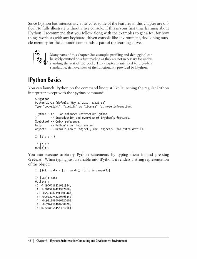
Since IPython has interactivity at its core, some of the features in this chapter are dif-ficult to fully illustrate without a live console. If this is your first time learning aboutIPython, I recommend that you follow along with the examples to get a feel for howthings work. As with any keyboard-driven console-like environment, developing mus-cle-memory for the common commands is part of the learning curve.
Many parts of this chapter (for example: profiling and debugging) canbe safely omitted on a first reading as they are not necessary for under-standing the rest of the book. This chapter is intended to provide astandalone, rich overview of the functionality provided by IPython.
IPython BasicsYou can launch IPython on the command line just like launching the regular Pythoninterpreter except with the ipython command:
$ ipythonPython 2.7.2 (default, May 27 2012, 21:26:12)Type "copyright", "credits" or "license" for more information.
IPython 0.12 -- An enhanced Interactive Python.? -> Introduction and overview of IPython's features.%quickref -> Quick reference.help -> Python's own help system.object? -> Details about 'object', use 'object??' for extra details.
In [1]: a = 5
In [2]: aOut[2]: 5
You can execute arbitrary Python statements by typing them in and pressing<return>. When typing just a variable into IPython, it renders a string representationof the object:
In [542]: data = {i : randn() for i in range(7)}
In [543]: dataOut[543]: {0: 0.6900018528091594, 1: 1.0015434424937888, 2: -0.5030873913603446, 3: -0.6222742250596455, 4: -0.9211686080130108, 5: -0.726213492660829, 6: 0.2228955458351768}
46 | Chapter 3: IPython: An Interactive Computing and Development Environment

Many kinds of Python objects are formatted to be more readable, or pretty-printed,which is distinct from normal printing with print. If you printed a dict like the abovein the standard Python interpreter, it would be much less readable:
>>> from numpy.random import randn>>> data = {i : randn() for i in range(7)}>>> print data{0: -1.5948255432744511, 1: 0.10569006472787983, 2: 1.972367135977295,3: 0.15455217573074576, 4: -0.24058577449429575, 5: -1.2904897053651216,6: 0.3308507317325902}
IPython also provides facilities to make it easy to execute arbitrary blocks of code (viasomewhat glorified copy-and-pasting) and whole Python scripts. These will be dis-cussed shortly.
Tab CompletionOn the surface, the IPython shell looks like a cosmetically slightly-different interactivePython interpreter. Users of Mathematica may find the enumerated input and outputprompts familiar. One of the major improvements over the standard Python shell istab completion, a feature common to most interactive data analysis environments.While entering expressions in the shell, pressing <Tab> will search the namespace forany variables (objects, functions, etc.) matching the characters you have typed so far:
In [1]: an_apple = 27
In [2]: an_example = 42
In [3]: an<Tab>an_apple and an_example any
In this example, note that IPython displayed both the two variables I defined as well asthe Python keyword and and built-in function any. Naturally, you can also completemethods and attributes on any object after typing a period:
In [3]: b = [1, 2, 3]
In [4]: b.<Tab>b.append b.extend b.insert b.remove b.sortb.count b.index b.pop b.reverse
The same goes for modules:
In [1]: import datetime
In [2]: datetime.<Tab>datetime.date datetime.MAXYEAR datetime.timedeltadatetime.datetime datetime.MINYEAR datetime.tzinfodatetime.datetime_CAPI datetime.time
IPython Basics | 47
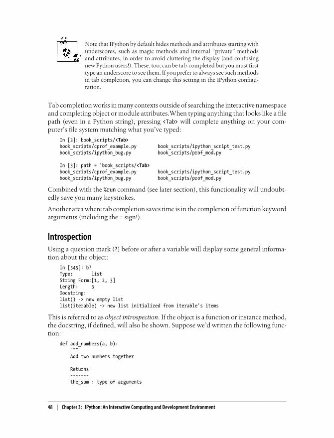
Note that IPython by default hides methods and attributes starting withunderscores, such as magic methods and internal “private” methodsand attributes, in order to avoid cluttering the display (and confusingnew Python users!). These, too, can be tab-completed but you must firsttype an underscore to see them. If you prefer to always see such methodsin tab completion, you can change this setting in the IPython configu-ration.
Tab completion works in many contexts outside of searching the interactive namespaceand completing object or module attributes.When typing anything that looks like a filepath (even in a Python string), pressing <Tab> will complete anything on your com-puter’s file system matching what you’ve typed:
In [3]: book_scripts/<Tab>book_scripts/cprof_example.py book_scripts/ipython_script_test.pybook_scripts/ipython_bug.py book_scripts/prof_mod.py
In [3]: path = 'book_scripts/<Tab>book_scripts/cprof_example.py book_scripts/ipython_script_test.pybook_scripts/ipython_bug.py book_scripts/prof_mod.py
Combined with the %run command (see later section), this functionality will undoubt-edly save you many keystrokes.
Another area where tab completion saves time is in the completion of function keywordarguments (including the = sign!).
IntrospectionUsing a question mark (?) before or after a variable will display some general informa-tion about the object:
In [545]: b?Type: listString Form:[1, 2, 3]Length: 3Docstring:list() -> new empty listlist(iterable) -> new list initialized from iterable's items
This is referred to as object introspection. If the object is a function or instance method,the docstring, if defined, will also be shown. Suppose we’d written the following func-tion:
def add_numbers(a, b): """ Add two numbers together
Returns ------- the_sum : type of arguments
48 | Chapter 3: IPython: An Interactive Computing and Development Environment

""" return a + b
Then using ? shows us the docstring:
In [547]: add_numbers?Type: functionString Form:<function add_numbers at 0x5fad848>File: book_scripts/<ipython-input-546-5473012eeb65>Definition: add_numbers(a, b)Docstring:Add two numbers togetherReturns-------the_sum : type of arguments
Using ?? will also show the function’s source code if possible:
In [548]: add_numbers??Type: functionString Form:<function add_numbers at 0x5fad848>File: book_scripts/<ipython-input-546-5473012eeb65>Definition: add_numbers(a, b)Source:def add_numbers(a, b): """ Add two numbers together Returns ------- the_sum : type of arguments """ return a + b
? has a final usage, which is for searching the IPython namespace in a manner similarto the standard UNIX or Windows command line. A number of characters combinedwith the wildcard (*) will show all names matching the wildcard expression. For ex-ample, we could get a list of all functions in the top level NumPy namespace containingload:
In [549]: np.*load*?np.loadnp.loadsnp.loadtxtnp.pkgload
The %run CommandAny file can be run as a Python program inside the environment of your IPython sessionusing the %run command. Suppose you had the following simple script stored in ipython_script_test.py:
def f(x, y, z): return (x + y) / z
a = 5
IPython Basics | 49
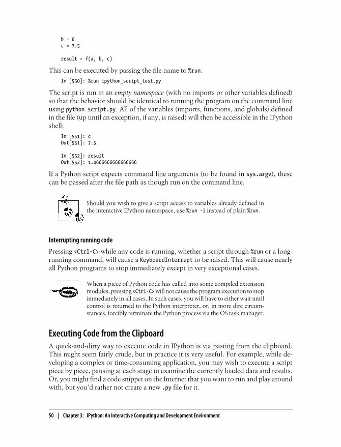
b = 6c = 7.5
result = f(a, b, c)
This can be executed by passing the file name to %run:
In [550]: %run ipython_script_test.py
The script is run in an empty namespace (with no imports or other variables defined)so that the behavior should be identical to running the program on the command lineusing python script.py. All of the variables (imports, functions, and globals) definedin the file (up until an exception, if any, is raised) will then be accessible in the IPythonshell:
In [551]: cOut[551]: 7.5
In [552]: resultOut[552]: 1.4666666666666666
If a Python script expects command line arguments (to be found in sys.argv), thesecan be passed after the file path as though run on the command line.
Should you wish to give a script access to variables already defined inthe interactive IPython namespace, use %run -i instead of plain %run.
Interrupting running code
Pressing <Ctrl-C> while any code is running, whether a script through %run or a long-running command, will cause a KeyboardInterrupt to be raised. This will cause nearlyall Python programs to stop immediately except in very exceptional cases.
When a piece of Python code has called into some compiled extensionmodules, pressing <Ctrl-C> will not cause the program execution to stopimmediately in all cases. In such cases, you will have to either wait untilcontrol is returned to the Python interpreter, or, in more dire circum-stances, forcibly terminate the Python process via the OS task manager.
Executing Code from the ClipboardA quick-and-dirty way to execute code in IPython is via pasting from the clipboard.This might seem fairly crude, but in practice it is very useful. For example, while de-veloping a complex or time-consuming application, you may wish to execute a scriptpiece by piece, pausing at each stage to examine the currently loaded data and results.Or, you might find a code snippet on the Internet that you want to run and play aroundwith, but you’d rather not create a new .py file for it.
50 | Chapter 3: IPython: An Interactive Computing and Development Environment

Code snippets can be pasted from the clipboard in many cases by pressing <Ctrl-Shift-V>. Note that it is not completely robust as this mode of pasting mimics typing eachline into IPython, and line breaks are treated as <return>. This means that if you pastecode with an indented block and there is a blank line, IPython will think that the in-dented block is over. Once the next line in the block is executed, an IndentationError will be raised. For example the following code:
x = 5y = 7if x > 5: x += 1
y = 8
will not work if simply pasted:
In [1]: x = 5
In [2]: y = 7
In [3]: if x > 5: ...: x += 1 ...:
In [4]: y = 8IndentationError: unexpected indent
If you want to paste code into IPython, try the %paste and %cpastemagic functions.
As the error message suggests, we should instead use the %paste and %cpaste magicfunctions. %paste takes whatever text is in the clipboard and executes it as a single blockin the shell:
In [6]: %pastex = 5y = 7if x > 5: x += 1
y = 8## -- End pasted text --
Depending on your platform and how you installed Python, there’s asmall chance that %paste will not work. Packaged distributions likeEPDFree (as described in in the intro) should not be a problem.
%cpaste is similar, except that it gives you a special prompt for pasting code into:
In [7]: %cpastePasting code; enter '--' alone on the line to stop or use Ctrl-D.:x = 5:y = 7:if x > 5:
IPython Basics | 51

: x += 1:: y = 8:--
With the %cpaste block, you have the freedom to paste as much code as you like beforeexecuting it. You might decide to use %cpaste in order to look at the pasted code beforeexecuting it. If you accidentally paste the wrong code, you can break out of the %cpaste prompt by pressing <Ctrl-C>.
Later, I’ll introduce the IPython HTML Notebook which brings a new level of sophis-tication for developing analyses block-by-block in a browser-based notebook formatwith executable code cells.
IPython interaction with editors and IDEs
Some text editors, such as Emacs and vim, have 3rd party extensions enabling blocksof code to be sent directly from the editor to a running IPython shell. Refer to theIPython website or do an Internet search to find out more.
Some IDEs, such as the PyDev plugin for Eclipse and Python Tools for Visual Studiofrom Microsoft (and possibly others), have integration with the IPython terminal ap-plication. If you want to work in an IDE but don’t want to give up the IPython consolefeatures, this may be a good option for you.
Keyboard ShortcutsIPython has many keyboard shortcuts for navigating the prompt (which will be familiarto users of the Emacs text editor or the UNIX bash shell) and interacting with the shell’scommand history (see later section). Table 3-1 summarizes some of the most commonlyused shortcuts. See Figure 3-1 for an illustration of a few of these, such as cursor move-ment.
Figure 3-1. Illustration of some of IPython’s keyboard shortcuts
52 | Chapter 3: IPython: An Interactive Computing and Development Environment

Table 3-1. Standard IPython Keyboard Shortcuts
Command Description
Ctrl-P or up-arrow Search backward in command history for commands starting with currently-entered text
Ctrl-N or down-arrow Search forward in command history for commands starting with currently-entered text
Ctrl-R Readline-style reverse history search (partial matching)
Ctrl-Shift-V Paste text from clipboard
Ctrl-C Interrupt currently-executing code
Ctrl-A Move cursor to beginning of line
Ctrl-E Move cursor to end of line
Ctrl-K Delete text from cursor until end of line
Ctrl-U Discard all text on current line
Ctrl-F Move cursor forward one character
Ctrl-B Move cursor back one character
Ctrl-L Clear screen
Exceptions and TracebacksIf an exception is raised while %run-ing a script or executing any statement, IPython willby default print a full call stack trace (traceback) with a few lines of context around theposition at each point in the stack.
In [553]: %run ch03/ipython_bug.py---------------------------------------------------------------------------AssertionError Traceback (most recent call last)/home/wesm/code/ipython/IPython/utils/py3compat.pyc in execfile(fname, *where) 176 else: 177 filename = fname--> 178 __builtin__.execfile(filename, *where)book_scripts/ch03/ipython_bug.py in <module>() 13 throws_an_exception() 14 ---> 15 calling_things()book_scripts/ch03/ipython_bug.py in calling_things() 11 def calling_things(): 12 works_fine()---> 13 throws_an_exception() 14 15 calling_things()book_scripts/ch03/ipython_bug.py in throws_an_exception() 7 a = 5 8 b = 6----> 9 assert(a + b == 10) 10 11 def calling_things():AssertionError:
IPython Basics | 53
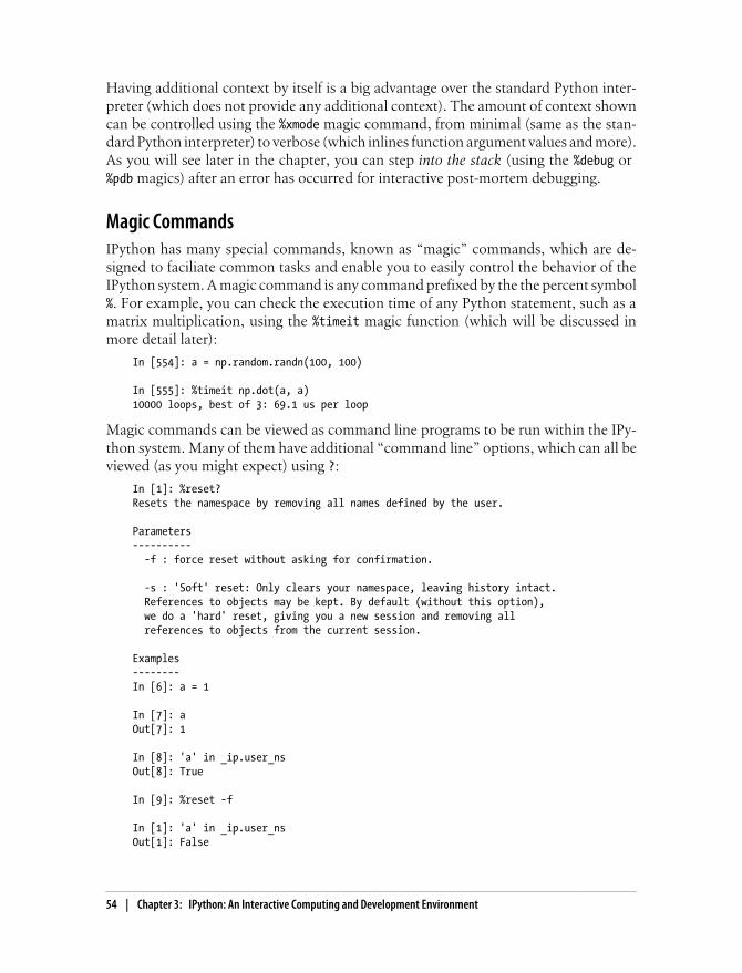
Having additional context by itself is a big advantage over the standard Python inter-preter (which does not provide any additional context). The amount of context showncan be controlled using the %xmode magic command, from minimal (same as the stan-dard Python interpreter) to verbose (which inlines function argument values and more).As you will see later in the chapter, you can step into the stack (using the %debug or %pdb magics) after an error has occurred for interactive post-mortem debugging.
Magic CommandsIPython has many special commands, known as “magic” commands, which are de-signed to faciliate common tasks and enable you to easily control the behavior of theIPython system. A magic command is any command prefixed by the the percent symbol%. For example, you can check the execution time of any Python statement, such as amatrix multiplication, using the %timeit magic function (which will be discussed inmore detail later):
In [554]: a = np.random.randn(100, 100)
In [555]: %timeit np.dot(a, a)10000 loops, best of 3: 69.1 us per loop
Magic commands can be viewed as command line programs to be run within the IPy-thon system. Many of them have additional “command line” options, which can all beviewed (as you might expect) using ?:
In [1]: %reset?Resets the namespace by removing all names defined by the user.
Parameters---------- -f : force reset without asking for confirmation.
-s : 'Soft' reset: Only clears your namespace, leaving history intact. References to objects may be kept. By default (without this option), we do a 'hard' reset, giving you a new session and removing all references to objects from the current session.
Examples--------In [6]: a = 1
In [7]: aOut[7]: 1
In [8]: 'a' in _ip.user_nsOut[8]: True
In [9]: %reset -f
In [1]: 'a' in _ip.user_nsOut[1]: False
54 | Chapter 3: IPython: An Interactive Computing and Development Environment
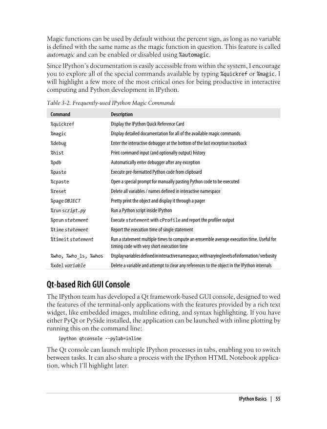
Magic functions can be used by default without the percent sign, as long as no variableis defined with the same name as the magic function in question. This feature is calledautomagic and can be enabled or disabled using %automagic.
Since IPython’s documentation is easily accessible from within the system, I encourageyou to explore all of the special commands available by typing %quickref or %magic. Iwill highlight a few more of the most critical ones for being productive in interactivecomputing and Python development in IPython.
Table 3-2. Frequently-used IPython Magic Commands
Command Description
%quickref Display the IPython Quick Reference Card
%magic Display detailed documentation for all of the available magic commands
%debug Enter the interactive debugger at the bottom of the last exception traceback
%hist Print command input (and optionally output) history
%pdb Automatically enter debugger after any exception
%paste Execute pre-formatted Python code from clipboard
%cpaste Open a special prompt for manually pasting Python code to be executed
%reset Delete all variables / names defined in interactive namespace
%page OBJECT Pretty print the object and display it through a pager
%run script.py Run a Python script inside IPython
%prun statement Execute statement with cProfile and report the profiler output
%time statement Report the execution time of single statement
%timeit statement Run a statement multiple times to compute an emsemble average execution time. Useful fortiming code with very short execution time
%who, %who_ls, %whos Display variables defined in interactive namespace, with varying levels of information / verbosity
%xdel variable Delete a variable and attempt to clear any references to the object in the IPython internals
Qt-based Rich GUI ConsoleThe IPython team has developed a Qt framework-based GUI console, designed to wedthe features of the terminal-only applications with the features provided by a rich textwidget, like embedded images, multiline editing, and syntax highlighting. If you haveeither PyQt or PySide installed, the application can be launched with inline plotting byrunning this on the command line:
ipython qtconsole --pylab=inline
The Qt console can launch multiple IPython processes in tabs, enabling you to switchbetween tasks. It can also share a process with the IPython HTML Notebook applica-tion, which I’ll highlight later.
IPython Basics | 55

Matplotlib Integration and Pylab ModePart of why IPython is so widely used in scientific computing is that it is designed as acompanion to libraries like matplotlib and other GUI toolkits. Don’t worry if you havenever used matplotlib before; it will be discussed in much more detail later in this book.If you create a matplotlib plot window in the regular Python shell, you’ll be sad to findthat the GUI event loop “takes control” of the Python session until the plot window isclosed. That won’t work for interactive data analysis and visualization, so IPython has
Figure 3-2. IPython Qt Console
56 | Chapter 3: IPython: An Interactive Computing and Development Environment

implemented special handling for each GUI framework so that it will work seamlesslywith the shell.
The typical way to launch IPython with matplotlib integration is by adding the --pylab flag (two dashes).
$ ipython --pylab
This will cause several things to happen. First IPython will launch with the default GUIbackend integration enabled so that matplotlib plot windows can be created with noissues. Secondly, most of NumPy and matplotlib will be imported into the top levelinteractive namespace to produce an interactive computing environment reminiscentof MATLAB and other domain-specific scientific computing environments. It’s possi-ble to do this setup by hand by using %gui, too (try running %gui? to find out how).
Figure 3-3. Pylab mode: IPython with matplotlib windows
IPython Basics | 57
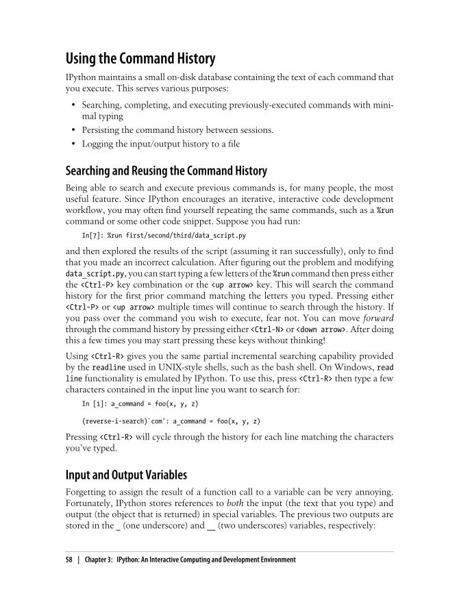
Using the Command HistoryIPython maintains a small on-disk database containing the text of each command thatyou execute. This serves various purposes:
• Searching, completing, and executing previously-executed commands with mini-mal typing
• Persisting the command history between sessions.
• Logging the input/output history to a file
Searching and Reusing the Command HistoryBeing able to search and execute previous commands is, for many people, the mostuseful feature. Since IPython encourages an iterative, interactive code developmentworkflow, you may often find yourself repeating the same commands, such as a %runcommand or some other code snippet. Suppose you had run:
In[7]: %run first/second/third/data_script.py
and then explored the results of the script (assuming it ran successfully), only to findthat you made an incorrect calculation. After figuring out the problem and modifyingdata_script.py, you can start typing a few letters of the %run command then press eitherthe <Ctrl-P> key combination or the <up arrow> key. This will search the commandhistory for the first prior command matching the letters you typed. Pressing either<Ctrl-P> or <up arrow> multiple times will continue to search through the history. Ifyou pass over the command you wish to execute, fear not. You can move forwardthrough the command history by pressing either <Ctrl-N> or <down arrow>. After doingthis a few times you may start pressing these keys without thinking!
Using <Ctrl-R> gives you the same partial incremental searching capability providedby the readline used in UNIX-style shells, such as the bash shell. On Windows, readline functionality is emulated by IPython. To use this, press <Ctrl-R> then type a fewcharacters contained in the input line you want to search for:
In [1]: a_command = foo(x, y, z)
(reverse-i-search)`com': a_command = foo(x, y, z)
Pressing <Ctrl-R> will cycle through the history for each line matching the charactersyou’ve typed.
Input and Output VariablesForgetting to assign the result of a function call to a variable can be very annoying.Fortunately, IPython stores references to both the input (the text that you type) andoutput (the object that is returned) in special variables. The previous two outputs arestored in the _ (one underscore) and __ (two underscores) variables, respectively:
58 | Chapter 3: IPython: An Interactive Computing and Development Environment
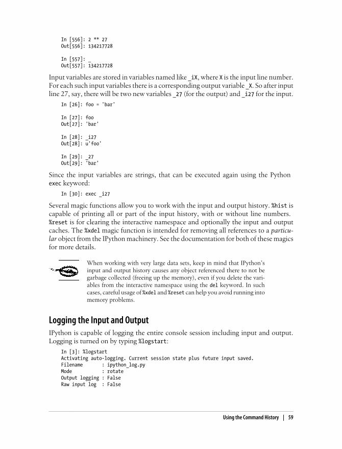
In [556]: 2 ** 27Out[556]: 134217728
In [557]: _Out[557]: 134217728
Input variables are stored in variables named like _iX, where X is the input line number.For each such input variables there is a corresponding output variable _X. So after inputline 27, say, there will be two new variables _27 (for the output) and _i27 for the input.
In [26]: foo = 'bar'
In [27]: fooOut[27]: 'bar'
In [28]: _i27Out[28]: u'foo'
In [29]: _27Out[29]: 'bar'
Since the input variables are strings, that can be executed again using the Python exec keyword:
In [30]: exec _i27
Several magic functions allow you to work with the input and output history. %hist iscapable of printing all or part of the input history, with or without line numbers. %reset is for clearing the interactive namespace and optionally the input and outputcaches. The %xdel magic function is intended for removing all references to a particu-lar object from the IPython machinery. See the documentation for both of these magicsfor more details.
When working with very large data sets, keep in mind that IPython’sinput and output history causes any object referenced there to not begarbage collected (freeing up the memory), even if you delete the vari-ables from the interactive namespace using the del keyword. In suchcases, careful usage of %xdel and %reset can help you avoid running intomemory problems.
Logging the Input and OutputIPython is capable of logging the entire console session including input and output.Logging is turned on by typing %logstart:
In [3]: %logstartActivating auto-logging. Current session state plus future input saved.Filename : ipython_log.pyMode : rotateOutput logging : FalseRaw input log : False
Using the Command History | 59

Timestamping : FalseState : active
IPython logging can be enabled at any time and it will record your entire session (in-cluding previous commands). Thus, if you are working on something and you decideyou want to save everything you did, you can simply enable logging. See the docstringof %logstart for more options (including changing the output file path), as well as thecompanion functions %logoff, %logon, %logstate, and %logstop.
Interacting with the Operating SystemAnother important feature of IPython is that it provides very strong integration withthe operating system shell. This means, among other things, that you can perform moststandard command line actions as you would in the Windows or UNIX (Linux, OS X)shell without having to exit IPython. This includes executing shell commands, changingdirectories, and storing the results of a command in a Python object (list or string).There are also simple shell command aliasing and directory bookmarking features.
See Table 3-3 for a summary of magic functions and syntax for calling shell commands.I’ll briefly visit these features in the next few sections.
Table 3-3. IPython system-related commands
Command Description
!cmd Execute cmd in the system shell
output = !cmd args Run cmd and store the stdout in output
%alias alias_name cmd Define an alias for a system (shell) command
%bookmark Utilize IPython’s directory bookmarking system
%cd directory Change system working directory to passed directory
%pwd Return the current system working directory
%pushd directory Place current directory on stack and change to target directory
%popd Change to directory popped off the top of the stack
%dirs Return a list containing the current directory stack
%dhist Print the history of visited directories
%env Return the system environment variables as a dict
Shell Commands and AliasesStarting a line in IPython with an exclamation point !, or bang, tells IPython to executeeverything after the bang in the system shell. This means that you can delete files (usingrm or del, depending on your OS), change directories, or execute any other process. It’seven possible to start processes that take control away from IPython, even anotherPython interpreter:
60 | Chapter 3: IPython: An Interactive Computing and Development Environment

In [2]: !pythonPython 2.7.2 |EPD 7.1-2 (64-bit)| (default, Jul 3 2011, 15:17:51)[GCC 4.1.2 20080704 (Red Hat 4.1.2-44)] on linux2Type "packages", "demo" or "enthought" for more information.>>>
The console output of a shell command can be stored in a variable by assigning the !-escaped expression to a variable. For example, on my Linux-based machine connectedto the Internet via ethernet, I can get my IP address as a Python variable:
In [1]: ip_info = !ifconfig eth0 | grep "inet "
In [2]: ip_info[0].strip()Out[2]: 'inet addr:192.168.1.137 Bcast:192.168.1.255 Mask:255.255.255.0'
The returned Python object ip_info is actually a custom list type containing variousversions of the console output.
IPython can also substitute in Python values defined in the current environment whenusing !. To do this, preface the variable name by the dollar sign $:
In [3]: foo = 'test*'
In [4]: !ls $footest4.py test.py test.xml
The %alias magic function can define custom shortcuts for shell commands. As a simpleexample:
In [1]: %alias ll ls -l
In [2]: ll /usrtotal 332drwxr-xr-x 2 root root 69632 2012-01-29 20:36 bin/drwxr-xr-x 2 root root 4096 2010-08-23 12:05 games/drwxr-xr-x 123 root root 20480 2011-12-26 18:08 include/drwxr-xr-x 265 root root 126976 2012-01-29 20:36 lib/drwxr-xr-x 44 root root 69632 2011-12-26 18:08 lib32/lrwxrwxrwx 1 root root 3 2010-08-23 16:02 lib64 -> lib/drwxr-xr-x 15 root root 4096 2011-10-13 19:03 local/drwxr-xr-x 2 root root 12288 2012-01-12 09:32 sbin/drwxr-xr-x 387 root root 12288 2011-11-04 22:53 share/drwxrwsr-x 24 root src 4096 2011-07-17 18:38 src/
Multiple commands can be executed just as on the command line by separating themwith semicolons:
In [558]: %alias test_alias (cd ch08; ls; cd ..)
In [559]: test_aliasmacrodata.csv spx.csv tips.csv
You’ll notice that IPython “forgets” any aliases you define interactively as soon as thesession is closed. To create permanent aliases, you will need to use the configurationsystem. See later in the chapter.
Interacting with the Operating System | 61

Directory Bookmark SystemIPython has a simple directory bookmarking system to enable you to save aliases forcommon directories so that you can jump around very easily. For example, I’m an aviduser of Dropbox, so I can define a bookmark to make it easy to change directories tomy Dropbox:
In [6]: %bookmark db /home/wesm/Dropbox/
Once I’ve done this, when I use the %cd magic, I can use any bookmarks I’ve defined
In [7]: cd db(bookmark:db) -> /home/wesm/Dropbox//home/wesm/Dropbox
If a bookmark name conflicts with a directory name in your current working directory,you can use the -b flag to override and use the bookmark location. Using the -l optionwith %bookmark lists all of your bookmarks:
In [8]: %bookmark -lCurrent bookmarks:db -> /home/wesm/Dropbox/
Bookmarks, unlike aliases, are automatically persisted between IPython sessions.
Software Development ToolsIn addition to being a comfortable environment for interactive computing and dataexploration, IPython is well suited as a software development environment. In dataanalysis applications, it’s important first to have correct code. Fortunately, IPython hasclosely integrated and enhanced the built-in Python pdb debugger. Secondly you wantyour code to be fast. For this IPython has easy-to-use code timing and profiling tools.I will give an overview of these tools in detail here.
Interactive DebuggerIPython’s debugger enhances pdb with tab completion, syntax highlighting, and contextfor each line in exception tracebacks. One of the best times to debug code is right afteran error has occurred. The %debug command, when entered immediately after an ex-ception, invokes the “post-mortem” debugger and drops you into the stack frame wherethe exception was raised:
In [2]: run ch03/ipython_bug.py---------------------------------------------------------------------------AssertionError Traceback (most recent call last)/home/wesm/book_scripts/ch03/ipython_bug.py in <module>() 13 throws_an_exception() 14---> 15 calling_things()
/home/wesm/book_scripts/ch03/ipython_bug.py in calling_things()
62 | Chapter 3: IPython: An Interactive Computing and Development Environment
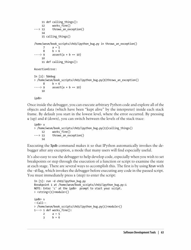
11 def calling_things(): 12 works_fine()---> 13 throws_an_exception() 14 15 calling_things()
/home/wesm/book_scripts/ch03/ipython_bug.py in throws_an_exception() 7 a = 5 8 b = 6----> 9 assert(a + b == 10) 10 11 def calling_things():
AssertionError:
In [3]: %debug> /home/wesm/book_scripts/ch03/ipython_bug.py(9)throws_an_exception() 8 b = 6----> 9 assert(a + b == 10) 10
ipdb>
Once inside the debugger, you can execute arbitrary Python code and explore all of theobjects and data (which have been “kept alive” by the interpreter) inside each stackframe. By default you start in the lowest level, where the error occurred. By pressingu (up) and d (down), you can switch between the levels of the stack trace:
ipdb> u> /home/wesm/book_scripts/ch03/ipython_bug.py(13)calling_things() 12 works_fine()---> 13 throws_an_exception() 14
Executing the %pdb command makes it so that IPython automatically invokes the de-bugger after any exception, a mode that many users will find especially useful.
It’s also easy to use the debugger to help develop code, especially when you wish to setbreakpoints or step through the execution of a function or script to examine the stateat each stage. There are several ways to accomplish this. The first is by using %run withthe -d flag, which invokes the debugger before executing any code in the passed script.You must immediately press s (step) to enter the script:
In [5]: run -d ch03/ipython_bug.pyBreakpoint 1 at /home/wesm/book_scripts/ch03/ipython_bug.py:1NOTE: Enter 'c' at the ipdb> prompt to start your script.> <string>(1)<module>()
ipdb> s--Call--> /home/wesm/book_scripts/ch03/ipython_bug.py(1)<module>()1---> 1 def works_fine(): 2 a = 5 3 b = 6
Software Development Tools | 63

After this point, it’s up to you how you want to work your way through the file. Forexample, in the above exception, we could set a breakpoint right before calling theworks_fine method and run the script until we reach the breakpoint by pressing c(continue):
ipdb> b 12ipdb> c> /home/wesm/book_scripts/ch03/ipython_bug.py(12)calling_things() 11 def calling_things():2--> 12 works_fine() 13 throws_an_exception()
At this point, you can step into works_fine() or execute works_fine() by pressing n(next) to advance to the next line:
ipdb> n> /home/wesm/book_scripts/ch03/ipython_bug.py(13)calling_things()2 12 works_fine()---> 13 throws_an_exception() 14
Then, we could step into throws_an_exception and advance to the line where the erroroccurs and look at the variables in the scope. Note that debugger commands takeprecedence over variable names; in such cases preface the variables with ! to examinetheir contents.
ipdb> s--Call--> /home/wesm/book_scripts/ch03/ipython_bug.py(6)throws_an_exception() 5----> 6 def throws_an_exception(): 7 a = 5
ipdb> n> /home/wesm/book_scripts/ch03/ipython_bug.py(7)throws_an_exception() 6 def throws_an_exception():----> 7 a = 5 8 b = 6
ipdb> n> /home/wesm/book_scripts/ch03/ipython_bug.py(8)throws_an_exception() 7 a = 5----> 8 b = 6 9 assert(a + b == 10)
ipdb> n> /home/wesm/book_scripts/ch03/ipython_bug.py(9)throws_an_exception() 8 b = 6----> 9 assert(a + b == 10) 10
ipdb> !a5ipdb> !b6
64 | Chapter 3: IPython: An Interactive Computing and Development Environment
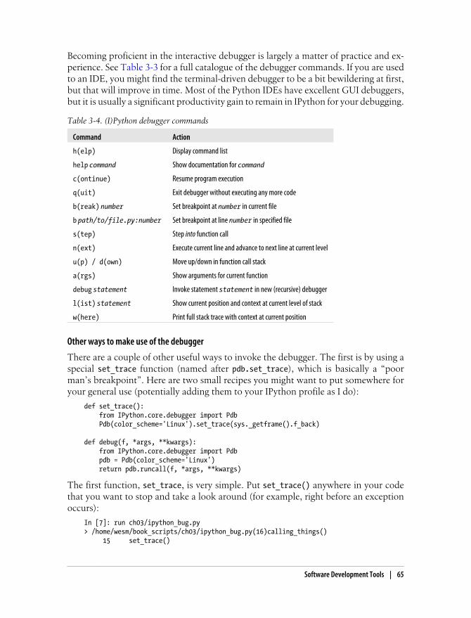
Becoming proficient in the interactive debugger is largely a matter of practice and ex-perience. See Table 3-3 for a full catalogue of the debugger commands. If you are usedto an IDE, you might find the terminal-driven debugger to be a bit bewildering at first,but that will improve in time. Most of the Python IDEs have excellent GUI debuggers,but it is usually a significant productivity gain to remain in IPython for your debugging.
Table 3-4. (I)Python debugger commands
Command Action
h(elp) Display command list
help command Show documentation for command
c(ontinue) Resume program execution
q(uit) Exit debugger without executing any more code
b(reak) number Set breakpoint at number in current file
b path/to/file.py:number Set breakpoint at line number in specified file
s(tep) Step into function call
n(ext) Execute current line and advance to next line at current level
u(p) / d(own) Move up/down in function call stack
a(rgs) Show arguments for current function
debug statement Invoke statement statement in new (recursive) debugger
l(ist) statement Show current position and context at current level of stack
w(here) Print full stack trace with context at current position
Other ways to make use of the debugger
There are a couple of other useful ways to invoke the debugger. The first is by using aspecial set_trace function (named after pdb.set_trace), which is basically a “poorman’s breakpoint”. Here are two small recipes you might want to put somewhere foryour general use (potentially adding them to your IPython profile as I do):
def set_trace(): from IPython.core.debugger import Pdb Pdb(color_scheme='Linux').set_trace(sys._getframe().f_back)
def debug(f, *args, **kwargs): from IPython.core.debugger import Pdb pdb = Pdb(color_scheme='Linux') return pdb.runcall(f, *args, **kwargs)
The first function, set_trace, is very simple. Put set_trace() anywhere in your codethat you want to stop and take a look around (for example, right before an exceptionoccurs):
In [7]: run ch03/ipython_bug.py> /home/wesm/book_scripts/ch03/ipython_bug.py(16)calling_things() 15 set_trace()
Software Development Tools | 65

---> 16 throws_an_exception() 17
Pressing c (continue) will cause the code to resume normally with no harm done.
The debug function above enables you to invoke the interactive debugger easily on anarbitrary function call. Suppose we had written a function like
def f(x, y, z=1): tmp = x + y return tmp / z
and we wished to step through its logic. Ordinarily using f would look like f(1, 2,z=3). To instead step into f, pass f as the first argument to debug followed by the po-sitional and keyword arguments to be passed to f:
In [6]: debug(f, 1, 2, z=3)> <ipython-input>(2)f() 1 def f(x, y, z):----> 2 tmp = x + y 3 return tmp / z
ipdb>
I find that these two simple recipes save me a lot of time on a day-to-day basis.
Lastly, the debugger can be used in conjunction with %run. By running a script with%run -d, you will be dropped directly into the debugger, ready to set any breakpointsand start the script:
In [1]: %run -d ch03/ipython_bug.pyBreakpoint 1 at /home/wesm/book_scripts/ch03/ipython_bug.py:1NOTE: Enter 'c' at the ipdb> prompt to start your script.> <string>(1)<module>()
ipdb>
Adding -b with a line number starts the debugger with a breakpoint set already:
In [2]: %run -d -b2 ch03/ipython_bug.pyBreakpoint 1 at /home/wesm/book_scripts/ch03/ipython_bug.py:2NOTE: Enter 'c' at the ipdb> prompt to start your script.> <string>(1)<module>()
ipdb> c> /home/wesm/book_scripts/ch03/ipython_bug.py(2)works_fine() 1 def works_fine():1---> 2 a = 5 3 b = 6
ipdb>
66 | Chapter 3: IPython: An Interactive Computing and Development Environment

Timing Code: %time and %timeitFor larger-scale or longer-running data analysis applications, you may wish to measurethe execution time of various components or of individual statements or function calls.You may want a report of which functions are taking up the most time in a complexprocess. Fortunately, IPython enables you to get this information very easily while youare developing and testing your code.
Timing code by hand using the built-in time module and its functions time.clock andtime.time is often tedious and repetitive, as you must write the same uninterestingboilerplate code:
import timestart = time.time()for i in range(iterations): # some code to run hereelapsed_per = (time.time() - start) / iterations
Since this is such a common operation, IPython has two magic functions %time and %timeit to automate this process for you. %time runs a statement once, reporting thetotal execution time. Suppose we had a large list of strings and we wanted to comparedifferent methods of selecting all strings starting with a particular prefix. Here is asimple list of 700,000 strings and two identical methods of selecting only the ones thatstart with 'foo':
# a very large list of stringsstrings = ['foo', 'foobar', 'baz', 'qux', 'python', 'Guido Van Rossum'] * 100000
method1 = [x for x in strings if x.startswith('foo')]
method2 = [x for x in strings if x[:3] == 'foo']
It looks like they should be about the same performance-wise, right? We can check forsure using %time:
In [561]: %time method1 = [x for x in strings if x.startswith('foo')]CPU times: user 0.19 s, sys: 0.00 s, total: 0.19 sWall time: 0.19 s
In [562]: %time method2 = [x for x in strings if x[:3] == 'foo']CPU times: user 0.09 s, sys: 0.00 s, total: 0.09 sWall time: 0.09 s
The Wall time is the main number of interest. So, it looks like the first method takesmore than twice as long, but it’s not a very precise measurement. If you try %time-ingthose statements multiple times yourself, you’ll find that the results are somewhatvariable. To get a more precise measurement, use the %timeit magic function. Givenan arbitrary statement, it has a heuristic to run a statement multiple times to producea fairly accurate average runtime.
In [563]: %timeit [x for x in strings if x.startswith('foo')]10 loops, best of 3: 159 ms per loop
Software Development Tools | 67

In [564]: %timeit [x for x in strings if x[:3] == 'foo']10 loops, best of 3: 59.3 ms per loop
This seemingly innocuous example illustrates that it is worth understanding the per-formance characteristics of the Python standard library, NumPy, pandas, and otherlibraries used in this book. In larger-scale data analysis applications, those millisecondswill start to add up!
%timeit is especially useful for analyzing statements and functions with very short ex-ecution times, even at the level of microseconds (1e-6 seconds) or nanoseconds (1e-9seconds). These may seem like insignificant amounts of time, but of course a 20 mi-crosecond function invoked 1 million times takes 15 seconds longer than a 5 micro-second function. In the above example, we could very directly compare the two stringoperations to understand their performance characteristics:
In [565]: x = 'foobar'
In [566]: y = 'foo'
In [567]: %timeit x.startswith(y)1000000 loops, best of 3: 267 ns per loop
In [568]: %timeit x[:3] == y10000000 loops, best of 3: 147 ns per loop
Basic Profiling: %prun and %run -pProfiling code is closely related to timing code, except it is concerned with determiningwhere time is spent. The main Python profiling tool is the cProfile module, which isnot specific to IPython at all. cProfile executes a program or any arbitrary block ofcode while keeping track of how much time is spent in each function.
A common way to use cProfile is on the command line, running an entire programand outputting the aggregated time per function. Suppose we had a simple script whichdoes some linear algebra in a loop (computing the maximum absolute eigenvalues ofa series of 100 x 100 matrices):
import numpy as npfrom numpy.linalg import eigvals
def run_experiment(niter=100): K = 100 results = [] for _ in xrange(niter): mat = np.random.randn(K, K) max_eigenvalue = np.abs(eigvals(mat)).max() results.append(max_eigenvalue) return resultssome_results = run_experiment()print 'Largest one we saw: %s' % np.max(some_results)
68 | Chapter 3: IPython: An Interactive Computing and Development Environment

Don’t worry if you are not familiar with NumPy. You can run this script throughcProfile by running the following in the command line:
python -m cProfile cprof_example.py
If you try that, you’ll find that the results are outputted sorted by function name. Thismakes it a bit hard to get an idea of where the most time is spent, so it’s very commonto specify a sort order using the -s flag:
$ python -m cProfile -s cumulative cprof_example.pyLargest one we saw: 11.923204422 15116 function calls (14927 primitive calls) in 0.720 seconds
Ordered by: cumulative time
ncalls tottime percall cumtime percall filename:lineno(function) 1 0.001 0.001 0.721 0.721 cprof_example.py:1(<module>) 100 0.003 0.000 0.586 0.006 linalg.py:702(eigvals) 200 0.572 0.003 0.572 0.003 {numpy.linalg.lapack_lite.dgeev} 1 0.002 0.002 0.075 0.075 __init__.py:106(<module>) 100 0.059 0.001 0.059 0.001 {method 'randn') 1 0.000 0.000 0.044 0.044 add_newdocs.py:9(<module>) 2 0.001 0.001 0.037 0.019 __init__.py:1(<module>) 2 0.003 0.002 0.030 0.015 __init__.py:2(<module>) 1 0.000 0.000 0.030 0.030 type_check.py:3(<module>) 1 0.001 0.001 0.021 0.021 __init__.py:15(<module>) 1 0.013 0.013 0.013 0.013 numeric.py:1(<module>) 1 0.000 0.000 0.009 0.009 __init__.py:6(<module>) 1 0.001 0.001 0.008 0.008 __init__.py:45(<module>) 262 0.005 0.000 0.007 0.000 function_base.py:3178(add_newdoc) 100 0.003 0.000 0.005 0.000 linalg.py:162(_assertFinite) ...
Only the first 15 rows of the output are shown. It’s easiest to read by scanning downthe cumtime column to see how much total time was spent inside each function. Notethat if a function calls some other function, the clock does not stop running. cProfilerecords the start and end time of each function call and uses that to produce the timing.
In addition to the above command-line usage, cProfile can also be used programmat-ically to profile arbitrary blocks of code without having to run a new process. IPythonhas a convenient interface to this capability using the %prun command and the -p optionto %run. %prun takes the same “command line options” as cProfile but will profile anarbitrary Python statement instead of a while .py file:
In [4]: %prun -l 7 -s cumulative run_experiment() 4203 function calls in 0.643 seconds
Ordered by: cumulative timeList reduced from 32 to 7 due to restriction <7>
ncalls tottime percall cumtime percall filename:lineno(function) 1 0.000 0.000 0.643 0.643 <string>:1(<module>) 1 0.001 0.001 0.643 0.643 cprof_example.py:4(run_experiment) 100 0.003 0.000 0.583 0.006 linalg.py:702(eigvals)
Software Development Tools | 69

200 0.569 0.003 0.569 0.003 {numpy.linalg.lapack_lite.dgeev} 100 0.058 0.001 0.058 0.001 {method 'randn'} 100 0.003 0.000 0.005 0.000 linalg.py:162(_assertFinite) 200 0.002 0.000 0.002 0.000 {method 'all' of 'numpy.ndarray' objects}
Similarly, calling %run -p -s cumulative cprof_example.py has the same effect as thecommand-line approach above, except you never have to leave IPython.
Profiling a Function Line-by-LineIn some cases the information you obtain from %prun (or another cProfile-based profilemethod) may not tell the whole story about a function’s execution time, or it may beso complex that the results, aggregated by function name, are hard to interpret. Forthis case, there is a small library called line_profiler (obtainable via PyPI or one of thepackage management tools). It contains an IPython extension enabling a new magicfunction %lprun that computes a line-by-line-profiling of one or more functions. Youcan enable this extension by modifying your IPython configuration (see the IPythondocumentation or the section on configuration later in this chapter) to include thefollowing line:
# A list of dotted module names of IPython extensions to load.c.TerminalIPythonApp.extensions = ['line_profiler']
line_profiler can be used programmatically (see the full documentation), but it isperhaps most powerful when used interactively in IPython. Suppose you had a moduleprof_mod with the following code doing some NumPy array operations:
from numpy.random import randn
def add_and_sum(x, y): added = x + y summed = added.sum(axis=1) return summed
def call_function(): x = randn(1000, 1000) y = randn(1000, 1000) return add_and_sum(x, y)
If we wanted to understand the performance of the add_and_sum function, %prun givesus the following:
In [569]: %run prof_mod
In [570]: x = randn(3000, 3000)
In [571]: y = randn(3000, 3000)
In [572]: %prun add_and_sum(x, y) 4 function calls in 0.049 seconds Ordered by: internal time ncalls tottime percall cumtime percall filename:lineno(function) 1 0.036 0.036 0.046 0.046 prof_mod.py:3(add_and_sum)
70 | Chapter 3: IPython: An Interactive Computing and Development Environment

1 0.009 0.009 0.009 0.009 {method 'sum' of 'numpy.ndarray' objects} 1 0.003 0.003 0.049 0.049 <string>:1(<module>) 1 0.000 0.000 0.000 0.000 {method 'disable' of '_lsprof.Profiler' objects}
This is not especially enlightening. With the line_profiler IPython extension activa-ted, a new command %lprun is available. The only difference in usage is that we mustinstruct %lprun which function or functions we wish to profile. The general syntax is:
%lprun -f func1 -f func2 statement_to_profile
In this case, we want to profile add_and_sum, so we run:
In [573]: %lprun -f add_and_sum add_and_sum(x, y)Timer unit: 1e-06 sFile: book_scripts/prof_mod.pyFunction: add_and_sum at line 3Total time: 0.045936 sLine # Hits Time Per Hit % Time Line Contents============================================================== 3 def add_and_sum(x, y): 4 1 36510 36510.0 79.5 added = x + y 5 1 9425 9425.0 20.5 summed = added.sum(axis=1) 6 1 1 1.0 0.0 return summed
You’ll probably agree this is much easier to interpret. In this case we profiled the samefunction we used in the statement. Looking at the module code above, we could callcall_function and profile that as well as add_and_sum, thus getting a full picture of theperformance of the code:
In [574]: %lprun -f add_and_sum -f call_function call_function()Timer unit: 1e-06 sFile: book_scripts/prof_mod.pyFunction: add_and_sum at line 3Total time: 0.005526 sLine # Hits Time Per Hit % Time Line Contents============================================================== 3 def add_and_sum(x, y): 4 1 4375 4375.0 79.2 added = x + y 5 1 1149 1149.0 20.8 summed = added.sum(axis=1) 6 1 2 2.0 0.0 return summedFile: book_scripts/prof_mod.pyFunction: call_function at line 8Total time: 0.121016 sLine # Hits Time Per Hit % Time Line Contents============================================================== 8 def call_function(): 9 1 57169 57169.0 47.2 x = randn(1000, 1000) 10 1 58304 58304.0 48.2 y = randn(1000, 1000) 11 1 5543 5543.0 4.6 return add_and_sum(x, y)
As a general rule of thumb, I tend to prefer %prun (cProfile) for “macro” profiling and%lprun (line_profiler) for “micro” profiling. It’s worthwhile to have a good under-standing of both tools.
Software Development Tools | 71

The reason that you have to specify explicitly the names of the functionsyou want to profile with %lprun is that the overhead of “tracing” theexecution time of each line is significant. Tracing functions that are notof interest would potentially significantly alter the profile results.
IPython HTML NotebookStarting in 2011, the IPython team, led by Brian Granger, built a web technology−basedinteractive computational document format that is commonly known as the IPythonNotebook. It has grown into a wonderful tool for interactive computing and an idealmedium for reproducible research and teaching. I’ve used it while writing most of theexamples in the book; I encourage you to make use of it, too.
It has a JSON-based .ipynb document format that enables easy sharing of code, output,and figures. Recently in Python conferences, a popular approach for demonstrationshas been to use the notebook and post the .ipynb files online afterward for everyoneto play with.
The notebook application runs as a lightweight server process on the command line.It can be started by running:
$ ipython notebook --pylab=inline[NotebookApp] Using existing profile dir: u'/home/wesm/.config/ipython/profile_default'[NotebookApp] Serving notebooks from /home/wesm/book_scripts[NotebookApp] The IPython Notebook is running at: http://127.0.0.1:8888/[NotebookApp] Use Control-C to stop this server and shut down all kernels.
On most platforms, your primary web browser will automatically open up to the note-book dashboard. In some cases you may have to navigate to the listed URL. From there,you can create a new notebook and start exploring.
Since you use the notebook inside a web browser, the server process can run anywhere.You can even securely connect to notebooks running on cloud service providers likeAmazon EC2. As of this writing, a new project NotebookCloud (http://notebookcloud.appspot.com) makes it easy to launch notebooks on EC2.
Tips for Productive Code Development Using IPythonWriting code in a way that makes it easy to develop, debug, and ultimately use inter-actively may be a paradigm shift for many users. There are procedural details like codereloading that may require some adjustment as well as coding style concerns.
As such, most of this section is more of an art than a science and will require someexperimentation on your part to determine a way to write your Python code that iseffective and productive for you. Ultimately you want to structure your code in a waythat makes it easy to use iteratively and to be able to explore the results of running aprogram or function as effortlessly as possible. I have found software designed with
72 | Chapter 3: IPython: An Interactive Computing and Development Environment

IPython in mind to be easier to work with than code intended only to be run as asstandalone command-line application. This becomes especially important when some-thing goes wrong and you have to diagnose an error in code that you or someone elsemight have written months or years beforehand.
Figure 3-4. IPython Notebook
Tips for Productive Code Development Using IPython | 73
Reloading Module DependenciesIn Python, when you type import some_lib, the code in some_lib is executed and all thevariables, functions, and imports defined within are stored in the newly createdsome_lib module namespace. The next time you type import some_lib, you will get areference to the existing module namespace. The potential difficulty in interactive codedevelopment in IPython comes when you, say, %run a script that depends on some othermodule where you may have made changes. Suppose I had the following code intest_script.py:
import some_lib
x = 5y = [1, 2, 3, 4]result = some_lib.get_answer(x, y)
If you were to execute %run test_script.py then modify some_lib.py, the next time youexecute %run test_script.py you will still get the old version of some_lib because ofPython’s “load-once” module system. This behavior differs from some other data anal-ysis environments, like MATLAB, which automatically propagate code changes.1 Tocope with this, you have a couple of options. The first way is to use Python's built-in reload function, altering test_script.py to look like the following:
import some_libreload(some_lib)
x = 5y = [1, 2, 3, 4]result = some_lib.get_answer(x, y)
This guarantees that you will get a fresh copy of some_lib every time you runtest_script.py. Obviously, if the dependencies go deeper, it might be a bit tricky to beinserting usages of reload all over the place. For this problem, IPython has a special dreload function (not a magic function) for “deep” (recursive) reloading of modules. IfI were to run import some_lib then type dreload(some_lib), it will attempt to reloadsome_lib as well as all of its dependencies. This will not work in all cases, unfortunately,but when it does it beats having to restart IPython.
Code Design TipsThere’s no simple recipe for this, but here are some high-level principles I have foundeffective in my own work.
1. Since a module or package may be imported in many different places in a particular program, Pythoncaches a module’s code the first time it is imported rather than executing the code in the module everytime. Otherwise, modularity and good code organization could potentially cause inefficiency in anapplication.
74 | Chapter 3: IPython: An Interactive Computing and Development Environment

Keep relevant objects and data alive
It’s not unusual to see a program written for the command line with a structure some-what like the following trivial example:
from my_functions import g
def f(x, y): return g(x + y)
def main(): x = 6 y = 7.5 result = x + y
if __name__ == '__main__': main()
Do you see what might be wrong with this program if we were to run it in IPython?After it’s done, none of the results or objects defined in the main function willl be ac-cessible in the IPython shell. A better way is to have whatever code is in main executedirectly in the module’s global namespace (or in the if __name__ == '__main__': block,if you want the module to also be importable). That way, when you %run the code,you’ll be able to look at all of the variables defined in main. It’s less meaningful in thissimple example, but in this book we’ll be looking at some complex data analysis prob-lems involving large data sets that you will want to be able to play with in IPython.
Flat is better than nested
Deeply nested code makes me think about the many layers of an onion. When testingor debugging a function, how many layers of the onion must you peel back in order toreach the code of interest? The idea that “flat is better than nested” is a part of the Zenof Python, and it applies generally to developing code for interactive use as well. Makingfunctions and classes as decoupled and modular as possible makes them easier to test(if you are writing unit tests), debug, and use interactively.
Overcome a fear of longer files
If you come from a Java (or another such language) background, you may have beentold to keep files short. In many languages, this is sound advice; long length is usuallya bad “code smell”, indicating refactoring or reorganization may be necessary. How-ever, while developing code using IPython, working with 10 small, but interconnectedfiles (under, say, 100 lines each) is likely to cause you more headache in general than asingle large file or two or three longer files. Fewer files means fewer modules to reloadand less jumping between files while editing, too. I have found maintaining largermodules, each with high internal cohesion, to be much more useful and pythonic. Afteriterating toward a solution, it sometimes will make sense to refactor larger files intosmaller ones.
Tips for Productive Code Development Using IPython | 75
Obviously, I don’t support taking this argument to the extreme, which would to be toput all of your code in a single monstrous file. Finding a sensible and intuitive moduleand package structure for a large codebase often takes a bit of work, but it is especiallyimportant to get right in teams. Each module should be internally cohesive, and itshould be as obvious as possible where to find functions and classes responsible foreach area of functionality.
Advanced IPython Features
Making Your Own Classes IPython-friendlyIPython makes every effort to display a console-friendly string representation of anyobject that you inspect. For many objects, like dicts, lists, and tuples, the built-in pprint module is used to do the nice formatting. In user-defined classes, however, youhave to generate the desired string output yourself. Suppose we had the following sim-ple class:
class Message: def __init__(self, msg): self.msg = msg
If you wrote this, you would be disappointed to discover that the default output foryour class isn’t very nice:
In [576]: x = Message('I have a secret')
In [577]: xOut[577]: <__main__.Message instance at 0x60ebbd8>
IPython takes the string returned by the __repr__ magic method (by doing output =repr(obj)) and prints that to the console. Thus, we can add a simple __repr__ methodto the above class to get a more helpful output:
class Message: def __init__(self, msg): self.msg = msg
def __repr__(self): return 'Message: %s' % self.msg
In [579]: x = Message('I have a secret')
In [580]: xOut[580]: Message: I have a secret
76 | Chapter 3: IPython: An Interactive Computing and Development Environment

Profiles and ConfigurationMost aspects of the appearance (colors, prompt, spacing between lines, etc.) and be-havior of the IPython shell are configurable through an extensive configuration system.Here are some of the things you can do via configuration:
• Change the color scheme
• Change how the input and output prompts look, or remove the blank line afterOut and before the next In prompt
• Change how the input and output prompts look
• Execute an arbitrary list of Python statements. These could be imports that youuse all the time or anything else you want to happen each time you launch IPython
• Enable IPython extensions, like the %lprun magic in line_profiler
• Define your own magics or system aliases
All of these configuration options are specified in a special ipython_config.py file whichwill be found in the ~/.config/ipython/ directory on UNIX-like systems and %HOME%/.ipython/ directory on Windows. Where your home directory is depends on yoursystem. Configuration is performed based on a particular profile. When you start IPy-thon normally, you load up, by default, the default profile, stored in the profile_default directory. Thus, on my Linux OS the full path to my default IPythonconfiguration file is:
/home/wesm/.config/ipython/profile_default/ipython_config.py
I’ll spare you the gory details of what’s in this file. Fortunately it has comments de-scribing what each configuration option is for, so I will leave it to the reader to tinkerand customize. One additional useful feature is that it’s possible to have multiple pro-files. Suppose you wanted to have an alternate IPython configuration tailored for aparticular application or project. Creating a new profile is as simple is typing somethinglike
ipython profile create secret_project
Once you’ve done this, edit the config files in the newly-created profile_secret_project directory then launch IPython like so
$ ipython --profile=secret_projectPython 2.7.2 |EPD 7.1-2 (64-bit)| (default, Jul 3 2011, 15:17:51)Type "copyright", "credits" or "license" for more information.
IPython 0.13 -- An enhanced Interactive Python.? -> Introduction and overview of IPython's features.%quickref -> Quick reference.help -> Python's own help system.object? -> Details about 'object', use 'object??' for extra details.
IPython profile: secret_project
Advanced IPython Features | 77
In [1]:
As always, the online IPython documentation is an excellent resource for more onprofiles and configuration.
CreditsParts of this chapter were derived from the wonderful documentation put together bythe IPython Development Team. I can’t thank them enough for all of their work build-ing this amazing set of tools.
78 | Chapter 3: IPython: An Interactive Computing and Development Environment
CHAPTER 4
NumPy Basics: Arrays and VectorizedComputation
NumPy, short for Numerical Python, is the fundamental package required for highperformance scientific computing and data analysis. It is the foundation on whichnearly all of the higher-level tools in this book are built. Here are some of the things itprovides:
• ndarray, a fast and space-efficient multidimensional array providing vectorizedarithmetic operations and sophisticated broadcasting capabilities
• Standard mathematical functions for fast operations on entire arrays of datawithout having to write loops
• Tools for reading / writing array data to disk and working with memory-mappedfiles
• Linear algebra, random number generation, and Fourier transform capabilities
• Tools for integrating code written in C, C++, and Fortran
The last bullet point is also one of the most important ones from an ecosystem pointof view. Because NumPy provides an easy-to-use C API, it is very easy to pass data toexternal libraries written in a low-level language and also for external libraries to returndata to Python as NumPy arrays. This feature has made Python a language of choicefor wrapping legacy C/C++/Fortran codebases and giving them a dynamic and easy-to-use interface.
While NumPy by itself does not provide very much high-level data analytical func-tionality, having an understanding of NumPy arrays and array-oriented computing willhelp you use tools like pandas much more effectively. If you’re new to Python and justlooking to get your hands dirty working with data using pandas, feel free to give thischapter a skim. For more on advanced NumPy features like broadcasting, see Chap-ter 12.
79

For most data analysis applications, the main areas of functionality I’ll focus on are:
• Fast vectorized array operations for data munging and cleaning, subsetting andfiltering, transformation, and any other kinds of computations
• Common array algorithms like sorting, unique, and set operations
• Efficient descriptive statistics and aggregating/summarizing data
• Data alignment and relational data manipulations for merging and joining togetherheterogeneous data sets
• Expressing conditional logic as array expressions instead of loops with if-elif-else branches
• Group-wise data manipulations (aggregation, transformation, function applica-tion). Much more on this in Chapter 5
While NumPy provides the computational foundation for these operations, you willlikely want to use pandas as your basis for most kinds of data analysis (especially forstructured or tabular data) as it provides a rich, high-level interface making most com-mon data tasks very concise and simple. pandas also provides some more domain-specific functionality like time series manipulation, which is not present in NumPy.
In this chapter and throughout the book, I use the standard NumPyconvention of always using import numpy as np. You are, of course,welcome to put from numpy import * in your code to avoid having towrite np., but I would caution you against making a habit of this.
The NumPy ndarray: A Multidimensional Array ObjectOne of the key features of NumPy is its N-dimensional array object, or ndarray, whichis a fast, flexible container for large data sets in Python. Arrays enable you to performmathematical operations on whole blocks of data using similar syntax to the equivalentoperations between scalar elements:
In [8]: dataOut[8]: array([[ 0.9526, -0.246 , -0.8856], [ 0.5639, 0.2379, 0.9104]])
In [9]: data * 10 In [10]: data + data Out[9]: Out[10]: array([[ 9.5256, -2.4601, -8.8565], array([[ 1.9051, -0.492 , -1.7713], [ 5.6385, 2.3794, 9.104 ]]) [ 1.1277, 0.4759, 1.8208]])
An ndarray is a generic multidimensional container for homogeneous data; that is, allof the elements must be the same type. Every array has a shape, a tuple indicating thesize of each dimension, and a dtype, an object describing the data type of the array:
In [11]: data.shapeOut[11]: (2, 3)
80 | Chapter 4: NumPy Basics: Arrays and Vectorized Computation
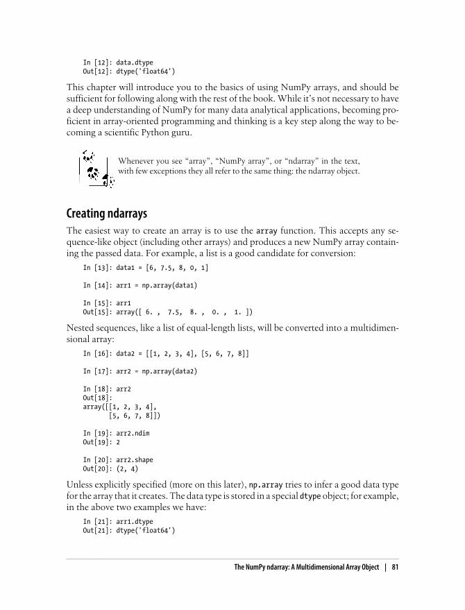
In [12]: data.dtypeOut[12]: dtype('float64')
This chapter will introduce you to the basics of using NumPy arrays, and should besufficient for following along with the rest of the book. While it’s not necessary to havea deep understanding of NumPy for many data analytical applications, becoming pro-ficient in array-oriented programming and thinking is a key step along the way to be-coming a scientific Python guru.
Whenever you see “array”, “NumPy array”, or “ndarray” in the text,with few exceptions they all refer to the same thing: the ndarray object.
Creating ndarraysThe easiest way to create an array is to use the array function. This accepts any se-quence-like object (including other arrays) and produces a new NumPy array contain-ing the passed data. For example, a list is a good candidate for conversion:
In [13]: data1 = [6, 7.5, 8, 0, 1]
In [14]: arr1 = np.array(data1)
In [15]: arr1Out[15]: array([ 6. , 7.5, 8. , 0. , 1. ])
Nested sequences, like a list of equal-length lists, will be converted into a multidimen-sional array:
In [16]: data2 = [[1, 2, 3, 4], [5, 6, 7, 8]]
In [17]: arr2 = np.array(data2)
In [18]: arr2Out[18]: array([[1, 2, 3, 4], [5, 6, 7, 8]])
In [19]: arr2.ndimOut[19]: 2
In [20]: arr2.shapeOut[20]: (2, 4)
Unless explicitly specified (more on this later), np.array tries to infer a good data typefor the array that it creates. The data type is stored in a special dtype object; for example,in the above two examples we have:
In [21]: arr1.dtypeOut[21]: dtype('float64')
The NumPy ndarray: A Multidimensional Array Object | 81
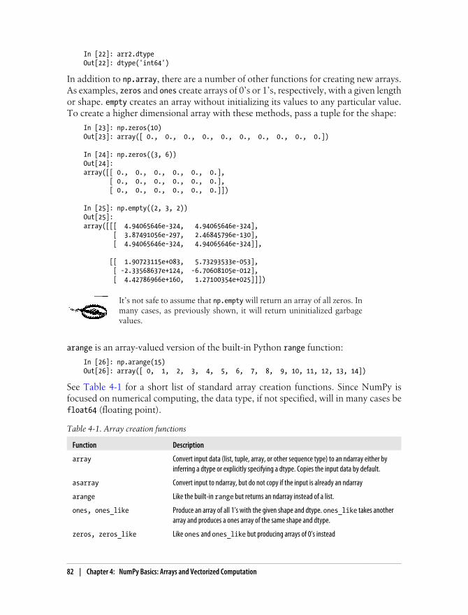
In [22]: arr2.dtypeOut[22]: dtype('int64')
In addition to np.array, there are a number of other functions for creating new arrays.As examples, zeros and ones create arrays of 0’s or 1’s, respectively, with a given lengthor shape. empty creates an array without initializing its values to any particular value.To create a higher dimensional array with these methods, pass a tuple for the shape:
In [23]: np.zeros(10)Out[23]: array([ 0., 0., 0., 0., 0., 0., 0., 0., 0., 0.])
In [24]: np.zeros((3, 6)) Out[24]: array([[ 0., 0., 0., 0., 0., 0.], [ 0., 0., 0., 0., 0., 0.], [ 0., 0., 0., 0., 0., 0.]])
In [25]: np.empty((2, 3, 2))Out[25]:array([[[ 4.94065646e-324, 4.94065646e-324], [ 3.87491056e-297, 2.46845796e-130], [ 4.94065646e-324, 4.94065646e-324]],
[[ 1.90723115e+083, 5.73293533e-053], [ -2.33568637e+124, -6.70608105e-012], [ 4.42786966e+160, 1.27100354e+025]]])
It’s not safe to assume that np.empty will return an array of all zeros. Inmany cases, as previously shown, it will return uninitialized garbagevalues.
arange is an array-valued version of the built-in Python range function:
In [26]: np.arange(15)Out[26]: array([ 0, 1, 2, 3, 4, 5, 6, 7, 8, 9, 10, 11, 12, 13, 14])
See Table 4-1 for a short list of standard array creation functions. Since NumPy isfocused on numerical computing, the data type, if not specified, will in many cases befloat64 (floating point).
Table 4-1. Array creation functions
Function Description
array Convert input data (list, tuple, array, or other sequence type) to an ndarray either byinferring a dtype or explicitly specifying a dtype. Copies the input data by default.
asarray Convert input to ndarray, but do not copy if the input is already an ndarray
arange Like the built-in range but returns an ndarray instead of a list.
ones, ones_like Produce an array of all 1’s with the given shape and dtype. ones_like takes anotherarray and produces a ones array of the same shape and dtype.
zeros, zeros_like Like ones and ones_like but producing arrays of 0’s instead
82 | Chapter 4: NumPy Basics: Arrays and Vectorized Computation

Function Description
empty, empty_like Create new arrays by allocating new memory, but do not populate with any values like ones and zeros
eye, identity Create a square N x N identity matrix (1’s on the diagonal and 0’s elsewhere)
Data Types for ndarraysThe data type or dtype is a special object containing the information the ndarray needsto interpret a chunk of memory as a particular type of data:
In [27]: arr1 = np.array([1, 2, 3], dtype=np.float64)
In [28]: arr2 = np.array([1, 2, 3], dtype=np.int32)
In [29]: arr1.dtype In [30]: arr2.dtype Out[29]: dtype('float64') Out[30]: dtype('int32')
Dtypes are part of what make NumPy so powerful and flexible. In most cases they mapdirectly onto an underlying machine representation, which makes it easy to read andwrite binary streams of data to disk and also to connect to code written in a low-levellanguage like C or Fortran. The numerical dtypes are named the same way: a type name,like float or int, followed by a number indicating the number of bits per element. Astandard double-precision floating point value (what’s used under the hood in Python’sfloat object) takes up 8 bytes or 64 bits. Thus, this type is known in NumPy asfloat64. See Table 4-2 for a full listing of NumPy’s supported data types.
Don’t worry about memorizing the NumPy dtypes, especially if you’rea new user. It’s often only necessary to care about the general kind ofdata you’re dealing with, whether floating point, complex, integer,boolean, string, or general Python object. When you need more controlover how data are stored in memory and on disk, especially large datasets, it is good to know that you have control over the storage type.
Table 4-2. NumPy data types
Type Type Code Description
int8, uint8 i1, u1 Signed and unsigned 8-bit (1 byte) integer types
int16, uint16 i2, u2 Signed and unsigned 16-bit integer types
int32, uint32 i4, u4 Signed and unsigned 32-bit integer types
int64, uint64 i8, u8 Signed and unsigned 32-bit integer types
float16 f2 Half-precision floating point
float32 f4 or f Standard single-precision floating point. Compatible with C float
float64, float128 f8 or d Standard double-precision floating point. Compatible with C doubleand Python float object
The NumPy ndarray: A Multidimensional Array Object | 83
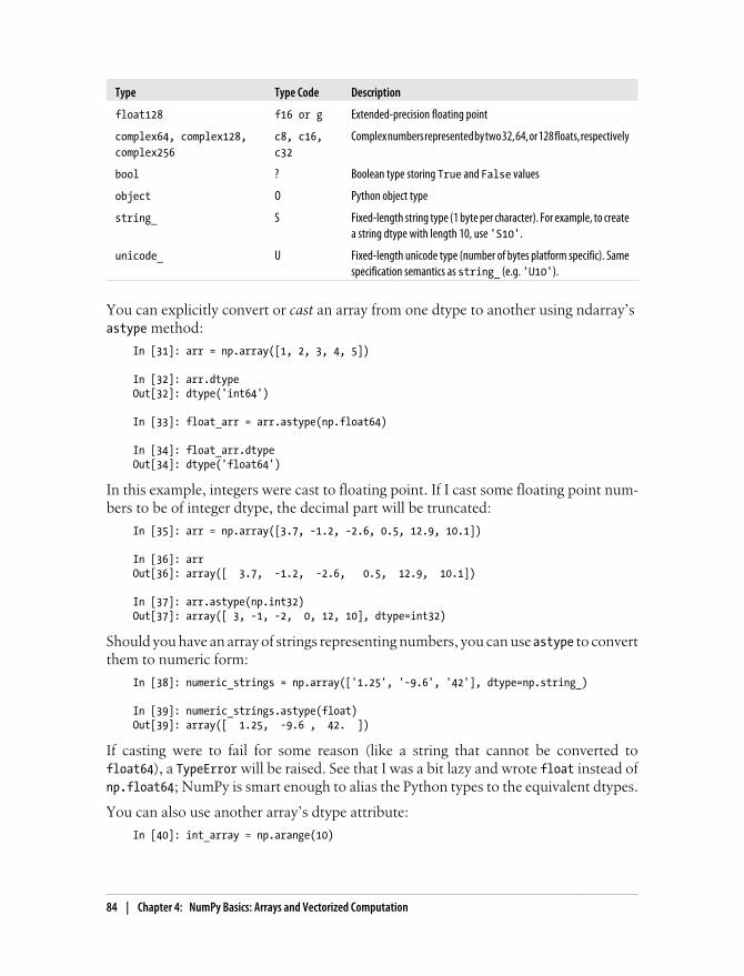
Type Type Code Description
float128 f16 or g Extended-precision floating point
complex64, complex128,complex256
c8, c16,c32
Complex numbers represented by two 32, 64, or 128 floats, respectively
bool ? Boolean type storing True and False values
object O Python object type
string_ S Fixed-length string type (1 byte per character). For example, to createa string dtype with length 10, use 'S10'.
unicode_ U Fixed-length unicode type (number of bytes platform specific). Samespecification semantics as string_ (e.g. 'U10').
You can explicitly convert or cast an array from one dtype to another using ndarray’s astype method:
In [31]: arr = np.array([1, 2, 3, 4, 5])
In [32]: arr.dtypeOut[32]: dtype('int64')
In [33]: float_arr = arr.astype(np.float64)
In [34]: float_arr.dtypeOut[34]: dtype('float64')
In this example, integers were cast to floating point. If I cast some floating point num-bers to be of integer dtype, the decimal part will be truncated:
In [35]: arr = np.array([3.7, -1.2, -2.6, 0.5, 12.9, 10.1])
In [36]: arrOut[36]: array([ 3.7, -1.2, -2.6, 0.5, 12.9, 10.1])
In [37]: arr.astype(np.int32)Out[37]: array([ 3, -1, -2, 0, 12, 10], dtype=int32)
Should you have an array of strings representing numbers, you can use astype to convertthem to numeric form:
In [38]: numeric_strings = np.array(['1.25', '-9.6', '42'], dtype=np.string_)
In [39]: numeric_strings.astype(float)Out[39]: array([ 1.25, -9.6 , 42. ])
If casting were to fail for some reason (like a string that cannot be converted tofloat64), a TypeError will be raised. See that I was a bit lazy and wrote float instead ofnp.float64; NumPy is smart enough to alias the Python types to the equivalent dtypes.
You can also use another array’s dtype attribute:
In [40]: int_array = np.arange(10)
84 | Chapter 4: NumPy Basics: Arrays and Vectorized Computation

In [41]: calibers = np.array([.22, .270, .357, .380, .44, .50], dtype=np.float64)
In [42]: int_array.astype(calibers.dtype)Out[42]: array([ 0., 1., 2., 3., 4., 5., 6., 7., 8., 9.])
There are shorthand type code strings you can also use to refer to a dtype:
In [43]: empty_uint32 = np.empty(8, dtype='u4')
In [44]: empty_uint32Out[44]: array([ 0, 0, 65904672, 0, 64856792, 0, 39438163, 0], dtype=uint32)
Calling astype always creates a new array (a copy of the data), even ifthe new dtype is the same as the old dtype.
It’s worth keeping in mind that floating point numbers, such as thosein float64 and float32 arrays, are only capable of approximating frac-tional quantities. In complex computations, you may accrue somefloating point error, making comparisons only valid up to a certain num-ber of decimal places.
Operations between Arrays and ScalarsArrays are important because they enable you to express batch operations on datawithout writing any for loops. This is usually called vectorization. Any arithmetic op-erations between equal-size arrays applies the operation elementwise:
In [45]: arr = np.array([[1., 2., 3.], [4., 5., 6.]])
In [46]: arrOut[46]: array([[ 1., 2., 3.], [ 4., 5., 6.]])
In [47]: arr * arr In [48]: arr - arr Out[47]: Out[48]: array([[ 1., 4., 9.], array([[ 0., 0., 0.], [ 16., 25., 36.]]) [ 0., 0., 0.]])
Arithmetic operations with scalars are as you would expect, propagating the value toeach element:
In [49]: 1 / arr In [50]: arr ** 0.5 Out[49]: Out[50]: array([[ 1. , 0.5 , 0.3333], array([[ 1. , 1.4142, 1.7321], [ 0.25 , 0.2 , 0.1667]]) [ 2. , 2.2361, 2.4495]])
The NumPy ndarray: A Multidimensional Array Object | 85
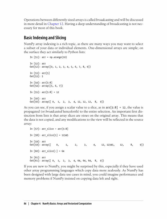
Operations between differently sized arrays is called broadcasting and will be discussedin more detail in Chapter 12. Having a deep understanding of broadcasting is not nec-essary for most of this book.
Basic Indexing and SlicingNumPy array indexing is a rich topic, as there are many ways you may want to selecta subset of your data or individual elements. One-dimensional arrays are simple; onthe surface they act similarly to Python lists:
In [51]: arr = np.arange(10)
In [52]: arrOut[52]: array([0, 1, 2, 3, 4, 5, 6, 7, 8, 9])
In [53]: arr[5]Out[53]: 5
In [54]: arr[5:8]Out[54]: array([5, 6, 7])
In [55]: arr[5:8] = 12
In [56]: arrOut[56]: array([ 0, 1, 2, 3, 4, 12, 12, 12, 8, 9])
As you can see, if you assign a scalar value to a slice, as in arr[5:8] = 12, the value ispropagated (or broadcasted henceforth) to the entire selection. An important first dis-tinction from lists is that array slices are views on the original array. This means thatthe data is not copied, and any modifications to the view will be reflected in the sourcearray:
In [57]: arr_slice = arr[5:8]
In [58]: arr_slice[1] = 12345
In [59]: arrOut[59]: array([ 0, 1, 2, 3, 4, 12, 12345, 12, 8, 9])
In [60]: arr_slice[:] = 64
In [61]: arrOut[61]: array([ 0, 1, 2, 3, 4, 64, 64, 64, 8, 9])
If you are new to NumPy, you might be surprised by this, especially if they have usedother array programming languages which copy data more zealously. As NumPy hasbeen designed with large data use cases in mind, you could imagine performance andmemory problems if NumPy insisted on copying data left and right.
86 | Chapter 4: NumPy Basics: Arrays and Vectorized Computation

If you want a copy of a slice of an ndarray instead of a view, you willneed to explicitly copy the array; for example arr[5:8].copy().
With higher dimensional arrays, you have many more options. In a two-dimensionalarray, the elements at each index are no longer scalars but rather one-dimensionalarrays:
In [62]: arr2d = np.array([[1, 2, 3], [4, 5, 6], [7, 8, 9]])
In [63]: arr2d[2]Out[63]: array([7, 8, 9])
Thus, individual elements can be accessed recursively. But that is a bit too much work,so you can pass a comma-separated list of indices to select individual elements. So theseare equivalent:
In [64]: arr2d[0][2]Out[64]: 3
In [65]: arr2d[0, 2]Out[65]: 3
See Figure 4-1 for an illustration of indexing on a 2D array.
Figure 4-1. Indexing elements in a NumPy array
In multidimensional arrays, if you omit later indices, the returned object will be a lower-dimensional ndarray consisting of all the data along the higher dimensions. So in the2 × 2 × 3 array arr3d
In [66]: arr3d = np.array([[[1, 2, 3], [4, 5, 6]], [[7, 8, 9], [10, 11, 12]]])
In [67]: arr3dOut[67]: array([[[ 1, 2, 3],
The NumPy ndarray: A Multidimensional Array Object | 87
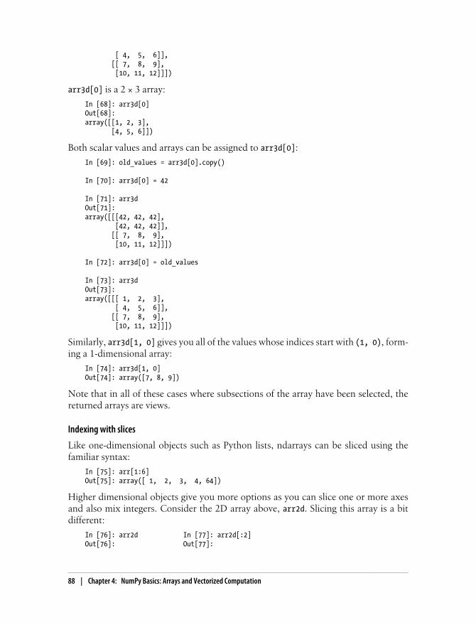
[ 4, 5, 6]], [[ 7, 8, 9], [10, 11, 12]]])
arr3d[0] is a 2 × 3 array:
In [68]: arr3d[0]Out[68]: array([[1, 2, 3], [4, 5, 6]])
Both scalar values and arrays can be assigned to arr3d[0]:
In [69]: old_values = arr3d[0].copy()
In [70]: arr3d[0] = 42
In [71]: arr3dOut[71]: array([[[42, 42, 42], [42, 42, 42]], [[ 7, 8, 9], [10, 11, 12]]])
In [72]: arr3d[0] = old_values
In [73]: arr3dOut[73]: array([[[ 1, 2, 3], [ 4, 5, 6]], [[ 7, 8, 9], [10, 11, 12]]])
Similarly, arr3d[1, 0] gives you all of the values whose indices start with (1, 0), form-ing a 1-dimensional array:
In [74]: arr3d[1, 0]Out[74]: array([7, 8, 9])
Note that in all of these cases where subsections of the array have been selected, thereturned arrays are views.
Indexing with slices
Like one-dimensional objects such as Python lists, ndarrays can be sliced using thefamiliar syntax:
In [75]: arr[1:6]Out[75]: array([ 1, 2, 3, 4, 64])
Higher dimensional objects give you more options as you can slice one or more axesand also mix integers. Consider the 2D array above, arr2d. Slicing this array is a bitdifferent:
In [76]: arr2d In [77]: arr2d[:2]Out[76]: Out[77]:
88 | Chapter 4: NumPy Basics: Arrays and Vectorized Computation

array([[1, 2, 3], array([[1, 2, 3], [4, 5, 6], [4, 5, 6]]) [7, 8, 9]])
As you can see, it has sliced along axis 0, the first axis. A slice, therefore, selects a rangeof elements along an axis. You can pass multiple slices just like you can pass multipleindexes:
In [78]: arr2d[:2, 1:]Out[78]: array([[2, 3], [5, 6]])
When slicing like this, you always obtain array views of the same number of dimensions.By mixing integer indexes and slices, you get lower dimensional slices:
In [79]: arr2d[1, :2] In [80]: arr2d[2, :1]Out[79]: array([4, 5]) Out[80]: array([7])
See Figure 4-2 for an illustration. Note that a colon by itself means to take the entireaxis, so you can slice only higher dimensional axes by doing:
In [81]: arr2d[:, :1]Out[81]: array([[1], [4], [7]])
Of course, assigning to a slice expression assigns to the whole selection:
In [82]: arr2d[:2, 1:] = 0
Boolean IndexingLet’s consider an example where we have some data in an array and an array of nameswith duplicates. I’m going to use here the randn function in numpy.random to generatesome random normally distributed data:
In [83]: names = np.array(['Bob', 'Joe', 'Will', 'Bob', 'Will', 'Joe', 'Joe'])
In [84]: data = randn(7, 4)
In [85]: namesOut[85]: array(['Bob', 'Joe', 'Will', 'Bob', 'Will', 'Joe', 'Joe'], dtype='|S4')
In [86]: dataOut[86]: array([[-0.048 , 0.5433, -0.2349, 1.2792], [-0.268 , 0.5465, 0.0939, -2.0445], [-0.047 , -2.026 , 0.7719, 0.3103], [ 2.1452, 0.8799, -0.0523, 0.0672], [-1.0023, -0.1698, 1.1503, 1.7289],
The NumPy ndarray: A Multidimensional Array Object | 89

[ 0.1913, 0.4544, 0.4519, 0.5535], [ 0.5994, 0.8174, -0.9297, -1.2564]])
Figure 4-2. Two-dimensional array slicing
Suppose each name corresponds to a row in the data array. If we wanted to select allthe rows with corresponding name 'Bob'. Like arithmetic operations, comparisons(such as ==) with arrays are also vectorized. Thus, comparing names with the string'Bob' yields a boolean array:
In [87]: names == 'Bob'Out[87]: array([ True, False, False, True, False, False, False], dtype=bool)
This boolean array can be passed when indexing the array:
In [88]: data[names == 'Bob']Out[88]: array([[-0.048 , 0.5433, -0.2349, 1.2792], [ 2.1452, 0.8799, -0.0523, 0.0672]])
The boolean array must be of the same length as the axis it’s indexing. You can evenmix and match boolean arrays with slices or integers (or sequences of integers, moreon this later):
In [89]: data[names == 'Bob', 2:]Out[89]: array([[-0.2349, 1.2792],
90 | Chapter 4: NumPy Basics: Arrays and Vectorized Computation

[-0.0523, 0.0672]])
In [90]: data[names == 'Bob', 3]Out[90]: array([ 1.2792, 0.0672])
To select everything but 'Bob', you can either use != or negate the condition using -:
In [91]: names != 'Bob'Out[91]: array([False, True, True, False, True, True, True], dtype=bool)
In [92]: data[-(names == 'Bob')]Out[92]: array([[-0.268 , 0.5465, 0.0939, -2.0445], [-0.047 , -2.026 , 0.7719, 0.3103], [-1.0023, -0.1698, 1.1503, 1.7289], [ 0.1913, 0.4544, 0.4519, 0.5535], [ 0.5994, 0.8174, -0.9297, -1.2564]])
Selecting two of the three names to combine multiple boolean conditions, use booleanarithmetic operators like & (and) and | (or):
In [93]: mask = (names == 'Bob') | (names == 'Will')
In [94]: maskOut[94]: array([True, False, True, True, True, False, False], dtype=bool)
In [95]: data[mask]Out[95]: array([[-0.048 , 0.5433, -0.2349, 1.2792], [-0.047 , -2.026 , 0.7719, 0.3103], [ 2.1452, 0.8799, -0.0523, 0.0672], [-1.0023, -0.1698, 1.1503, 1.7289]])
Selecting data from an array by boolean indexing always creates a copy of the data,even if the returned array is unchanged.
The Python keywords and and or do not work with boolean arrays.
Setting values with boolean arrays works in a common-sense way. To set all of thenegative values in data to 0 we need only do:
In [96]: data[data < 0] = 0
In [97]: dataOut[97]: array([[ 0. , 0.5433, 0. , 1.2792], [ 0. , 0.5465, 0.0939, 0. ], [ 0. , 0. , 0.7719, 0.3103], [ 2.1452, 0.8799, 0. , 0.0672], [ 0. , 0. , 1.1503, 1.7289], [ 0.1913, 0.4544, 0.4519, 0.5535], [ 0.5994, 0.8174, 0. , 0. ]])
The NumPy ndarray: A Multidimensional Array Object | 91

Setting whole rows or columns using a 1D boolean array is also easy:
In [98]: data[names != 'Joe'] = 7
In [99]: dataOut[99]: array([[ 7. , 7. , 7. , 7. ], [ 0. , 0.5465, 0.0939, 0. ], [ 7. , 7. , 7. , 7. ], [ 7. , 7. , 7. , 7. ], [ 7. , 7. , 7. , 7. ], [ 0.1913, 0.4544, 0.4519, 0.5535], [ 0.5994, 0.8174, 0. , 0. ]])
Fancy IndexingFancy indexing is a term adopted by NumPy to describe indexing using integer arrays.Suppose we had a 8 × 4 array:
In [100]: arr = np.empty((8, 4))
In [101]: for i in range(8): .....: arr[i] = i
In [102]: arrOut[102]: array([[ 0., 0., 0., 0.], [ 1., 1., 1., 1.], [ 2., 2., 2., 2.], [ 3., 3., 3., 3.], [ 4., 4., 4., 4.], [ 5., 5., 5., 5.], [ 6., 6., 6., 6.], [ 7., 7., 7., 7.]])
To select out a subset of the rows in a particular order, you can simply pass a list orndarray of integers specifying the desired order:
In [103]: arr[[4, 3, 0, 6]]Out[103]: array([[ 4., 4., 4., 4.], [ 3., 3., 3., 3.], [ 0., 0., 0., 0.], [ 6., 6., 6., 6.]])
Hopefully this code did what you expected! Using negative indices select rows fromthe end:
In [104]: arr[[-3, -5, -7]]Out[104]: array([[ 5., 5., 5., 5.], [ 3., 3., 3., 3.], [ 1., 1., 1., 1.]])
92 | Chapter 4: NumPy Basics: Arrays and Vectorized Computation
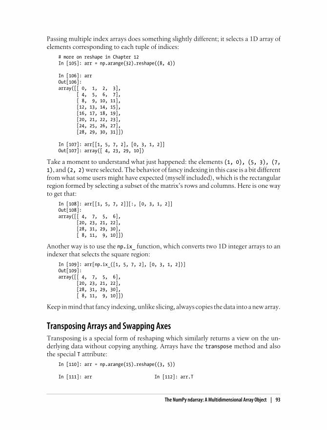
Passing multiple index arrays does something slightly different; it selects a 1D array ofelements corresponding to each tuple of indices:
# more on reshape in Chapter 12In [105]: arr = np.arange(32).reshape((8, 4))
In [106]: arrOut[106]: array([[ 0, 1, 2, 3], [ 4, 5, 6, 7], [ 8, 9, 10, 11], [12, 13, 14, 15], [16, 17, 18, 19], [20, 21, 22, 23], [24, 25, 26, 27], [28, 29, 30, 31]])
In [107]: arr[[1, 5, 7, 2], [0, 3, 1, 2]]Out[107]: array([ 4, 23, 29, 10])
Take a moment to understand what just happened: the elements (1, 0), (5, 3), (7,1), and (2, 2) were selected. The behavior of fancy indexing in this case is a bit differentfrom what some users might have expected (myself included), which is the rectangularregion formed by selecting a subset of the matrix’s rows and columns. Here is one wayto get that:
In [108]: arr[[1, 5, 7, 2]][:, [0, 3, 1, 2]]Out[108]: array([[ 4, 7, 5, 6], [20, 23, 21, 22], [28, 31, 29, 30], [ 8, 11, 9, 10]])
Another way is to use the np.ix_ function, which converts two 1D integer arrays to anindexer that selects the square region:
In [109]: arr[np.ix_([1, 5, 7, 2], [0, 3, 1, 2])]Out[109]: array([[ 4, 7, 5, 6], [20, 23, 21, 22], [28, 31, 29, 30], [ 8, 11, 9, 10]])
Keep in mind that fancy indexing, unlike slicing, always copies the data into a new array.
Transposing Arrays and Swapping AxesTransposing is a special form of reshaping which similarly returns a view on the un-derlying data without copying anything. Arrays have the transpose method and alsothe special T attribute:
In [110]: arr = np.arange(15).reshape((3, 5))
In [111]: arr In [112]: arr.T
The NumPy ndarray: A Multidimensional Array Object | 93

Out[111]: Out[112]: array([[ 0, 1, 2, 3, 4], array([[ 0, 5, 10], [ 5, 6, 7, 8, 9], [ 1, 6, 11], [10, 11, 12, 13, 14]]) [ 2, 7, 12], [ 3, 8, 13], [ 4, 9, 14]])
When doing matrix computations, you will do this very often, like for example com-puting the inner matrix product XTX using np.dot:
In [113]: arr = np.random.randn(6, 3)
In [114]: np.dot(arr.T, arr)Out[114]: array([[ 2.584 , 1.8753, 0.8888], [ 1.8753, 6.6636, 0.3884], [ 0.8888, 0.3884, 3.9781]])
For higher dimensional arrays, transpose will accept a tuple of axis numbers to permutethe axes (for extra mind bending):
In [115]: arr = np.arange(16).reshape((2, 2, 4))
In [116]: arrOut[116]: array([[[ 0, 1, 2, 3], [ 4, 5, 6, 7]], [[ 8, 9, 10, 11], [12, 13, 14, 15]]])
In [117]: arr.transpose((1, 0, 2))Out[117]: array([[[ 0, 1, 2, 3], [ 8, 9, 10, 11]], [[ 4, 5, 6, 7], [12, 13, 14, 15]]])
Simple transposing with .T is just a special case of swapping axes. ndarray has themethod swapaxes which takes a pair of axis numbers:
In [118]: arr In [119]: arr.swapaxes(1, 2)Out[118]: Out[119]: array([[[ 0, 1, 2, 3], array([[[ 0, 4], [ 4, 5, 6, 7]], [ 1, 5], [ 2, 6], [[ 8, 9, 10, 11], [ 3, 7]], [12, 13, 14, 15]]]) [[ 8, 12], [ 9, 13], [10, 14], [11, 15]]])
swapaxes similarly returns a view on the data without making a copy.
94 | Chapter 4: NumPy Basics: Arrays and Vectorized Computation

Universal Functions: Fast Element-wise Array FunctionsA universal function, or ufunc, is a function that performs elementwise operations ondata in ndarrays. You can think of them as fast vectorized wrappers for simple functionsthat take one or more scalar values and produce one or more scalar results.
Many ufuncs are simple elementwise transformations, like sqrt or exp:
In [120]: arr = np.arange(10)
In [121]: np.sqrt(arr)Out[121]: array([ 0. , 1. , 1.4142, 1.7321, 2. , 2.2361, 2.4495, 2.6458, 2.8284, 3. ])
In [122]: np.exp(arr)Out[122]: array([ 1. , 2.7183, 7.3891, 20.0855, 54.5982, 148.4132, 403.4288, 1096.6332, 2980.958 , 8103.0839])
These are referred to as unary ufuncs. Others, such as add or maximum, take 2 arrays(thus, binary ufuncs) and return a single array as the result:
In [123]: x = randn(8)
In [124]: y = randn(8)
In [125]: xOut[125]: array([ 0.0749, 0.0974, 0.2002, -0.2551, 0.4655, 0.9222, 0.446 , -0.9337])
In [126]: yOut[126]: array([ 0.267 , -1.1131, -0.3361, 0.6117, -1.2323, 0.4788, 0.4315, -0.7147])
In [127]: np.maximum(x, y) # element-wise maximumOut[127]: array([ 0.267 , 0.0974, 0.2002, 0.6117, 0.4655, 0.9222, 0.446 , -0.7147])
While not common, a ufunc can return multiple arrays. modf is one example, a vector-ized version of the built-in Python divmod: it returns the fractional and integral parts ofa floating point array:
In [128]: arr = randn(7) * 5
In [129]: np.modf(arr)Out[129]: (array([-0.6808, 0.0636, -0.386 , 0.1393, -0.8806, 0.9363, -0.883 ]), array([-2., 4., -3., 5., -3., 3., -6.]))
Universal Functions: Fast Element-wise Array Functions | 95

See Table 4-3 and Table 4-4 for a listing of available ufuncs.
Table 4-3. Unary ufuncs
Function Description
abs, fabs Compute the absolute value element-wise for integer, floating point, or complex values.Use fabs as a faster alternative for non-complex-valued data
sqrt Compute the square root of each element. Equivalent to arr ** 0.5
square Compute the square of each element. Equivalent to arr ** 2
exp Compute the exponent ex of each element
log, log10, log2, log1p Natural logarithm (base e), log base 10, log base 2, and log(1 + x), respectively
sign Compute the sign of each element: 1 (positive), 0 (zero), or -1 (negative)
ceil Compute the ceiling of each element, i.e. the smallest integer greater than or equal toeach element
floor Compute the floor of each element, i.e. the largest integer less than or equal to eachelement
rint Round elements to the nearest integer, preserving the dtype
modf Return fractional and integral parts of array as separate array
isnan Return boolean array indicating whether each value is NaN (Not a Number)
isfinite, isinf Return boolean array indicating whether each element is finite (non-inf, non-NaN) orinfinite, respectively
cos, cosh, sin, sinh,tan, tanh
Regular and hyperbolic trigonometric functions
arccos, arccosh, arcsin,arcsinh, arctan, arctanh
Inverse trigonometric functions
logical_not Compute truth value of not x element-wise. Equivalent to -arr.
Table 4-4. Binary universal functions
Function Description
add Add corresponding elements in arrays
subtract Subtract elements in second array from first array
multiply Multiply array elements
divide, floor_divide Divide or floor divide (truncating the remainder)
power Raise elements in first array to powers indicated in second array
maximum, fmax Element-wise maximum. fmax ignores NaN
minimum, fmin Element-wise minimum. fmin ignores NaN
mod Element-wise modulus (remainder of division)
copysign Copy sign of values in second argument to values in first argument
96 | Chapter 4: NumPy Basics: Arrays and Vectorized Computation
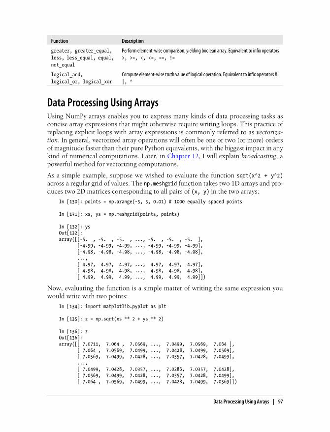
Function Description
greater, greater_equal,less, less_equal, equal,not_equal
Perform element-wise comparison, yielding boolean array. Equivalent to infix operators>, >=, <, <=, ==, !=
logical_and,logical_or, logical_xor
Compute element-wise truth value of logical operation. Equivalent to infix operators &|, ^
Data Processing Using ArraysUsing NumPy arrays enables you to express many kinds of data processing tasks asconcise array expressions that might otherwise require writing loops. This practice ofreplacing explicit loops with array expressions is commonly referred to as vectoriza-tion. In general, vectorized array operations will often be one or two (or more) ordersof magnitude faster than their pure Python equivalents, with the biggest impact in anykind of numerical computations. Later, in Chapter 12, I will explain broadcasting, apowerful method for vectorizing computations.
As a simple example, suppose we wished to evaluate the function sqrt(x^2 + y^2)across a regular grid of values. The np.meshgrid function takes two 1D arrays and pro-duces two 2D matrices corresponding to all pairs of (x, y) in the two arrays:
In [130]: points = np.arange(-5, 5, 0.01) # 1000 equally spaced points
In [131]: xs, ys = np.meshgrid(points, points)
In [132]: ysOut[132]: array([[-5. , -5. , -5. , ..., -5. , -5. , -5. ], [-4.99, -4.99, -4.99, ..., -4.99, -4.99, -4.99], [-4.98, -4.98, -4.98, ..., -4.98, -4.98, -4.98], ..., [ 4.97, 4.97, 4.97, ..., 4.97, 4.97, 4.97], [ 4.98, 4.98, 4.98, ..., 4.98, 4.98, 4.98], [ 4.99, 4.99, 4.99, ..., 4.99, 4.99, 4.99]])
Now, evaluating the function is a simple matter of writing the same expression youwould write with two points:
In [134]: import matplotlib.pyplot as plt
In [135]: z = np.sqrt(xs ** 2 + ys ** 2)
In [136]: zOut[136]: array([[ 7.0711, 7.064 , 7.0569, ..., 7.0499, 7.0569, 7.064 ], [ 7.064 , 7.0569, 7.0499, ..., 7.0428, 7.0499, 7.0569], [ 7.0569, 7.0499, 7.0428, ..., 7.0357, 7.0428, 7.0499], ..., [ 7.0499, 7.0428, 7.0357, ..., 7.0286, 7.0357, 7.0428], [ 7.0569, 7.0499, 7.0428, ..., 7.0357, 7.0428, 7.0499], [ 7.064 , 7.0569, 7.0499, ..., 7.0428, 7.0499, 7.0569]])
Data Processing Using Arrays | 97
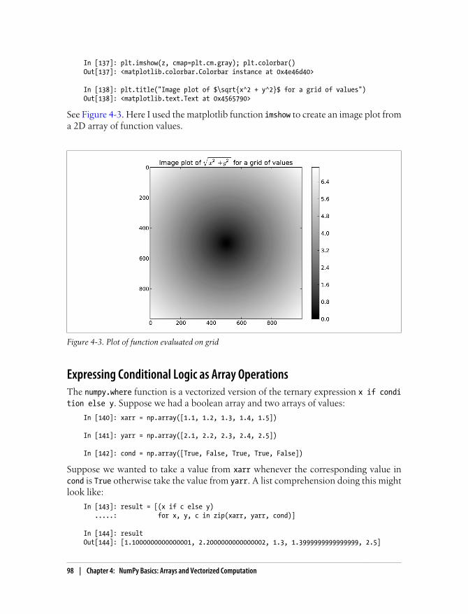
In [137]: plt.imshow(z, cmap=plt.cm.gray); plt.colorbar()Out[137]: <matplotlib.colorbar.Colorbar instance at 0x4e46d40>
In [138]: plt.title("Image plot of $\sqrt{x^2 + y^2}$ for a grid of values")Out[138]: <matplotlib.text.Text at 0x4565790>
See Figure 4-3. Here I used the matplotlib function imshow to create an image plot froma 2D array of function values.
Figure 4-3. Plot of function evaluated on grid
Expressing Conditional Logic as Array OperationsThe numpy.where function is a vectorized version of the ternary expression x if condition else y. Suppose we had a boolean array and two arrays of values:
In [140]: xarr = np.array([1.1, 1.2, 1.3, 1.4, 1.5])
In [141]: yarr = np.array([2.1, 2.2, 2.3, 2.4, 2.5])
In [142]: cond = np.array([True, False, True, True, False])
Suppose we wanted to take a value from xarr whenever the corresponding value incond is True otherwise take the value from yarr. A list comprehension doing this mightlook like:
In [143]: result = [(x if c else y) .....: for x, y, c in zip(xarr, yarr, cond)]
In [144]: resultOut[144]: [1.1000000000000001, 2.2000000000000002, 1.3, 1.3999999999999999, 2.5]
98 | Chapter 4: NumPy Basics: Arrays and Vectorized Computation

This has multiple problems. First, it will not be very fast for large arrays (because allthe work is being done in pure Python). Secondly, it will not work with multidimen-sional arrays. With np.where you can write this very concisely:
In [145]: result = np.where(cond, xarr, yarr)
In [146]: resultOut[146]: array([ 1.1, 2.2, 1.3, 1.4, 2.5])
The second and third arguments to np.where don’t need to be arrays; one or both ofthem can be scalars. A typical use of where in data analysis is to produce a new array ofvalues based on another array. Suppose you had a matrix of randomly generated dataand you wanted to replace all positive values with 2 and all negative values with -2.This is very easy to do with np.where:
In [147]: arr = randn(4, 4)
In [148]: arrOut[148]: array([[ 0.6372, 2.2043, 1.7904, 0.0752], [-1.5926, -1.1536, 0.4413, 0.3483], [-0.1798, 0.3299, 0.7827, -0.7585], [ 0.5857, 0.1619, 1.3583, -1.3865]])
In [149]: np.where(arr > 0, 2, -2)Out[149]: array([[ 2, 2, 2, 2], [-2, -2, 2, 2], [-2, 2, 2, -2], [ 2, 2, 2, -2]])
In [150]: np.where(arr > 0, 2, arr) # set only positive values to 2Out[150]: array([[ 2. , 2. , 2. , 2. ], [-1.5926, -1.1536, 2. , 2. ], [-0.1798, 2. , 2. , -0.7585], [ 2. , 2. , 2. , -1.3865]])
The arrays passed to where can be more than just equal sizes array or scalers.
With some cleverness you can use where to express more complicated logic; considerthis example where I have two boolean arrays, cond1 and cond2, and wish to assign adifferent value for each of the 4 possible pairs of boolean values:
result = []for i in range(n): if cond1[i] and cond2[i]: result.append(0) elif cond1[i]: result.append(1) elif cond2[i]: result.append(2) else: result.append(3)
Data Processing Using Arrays | 99
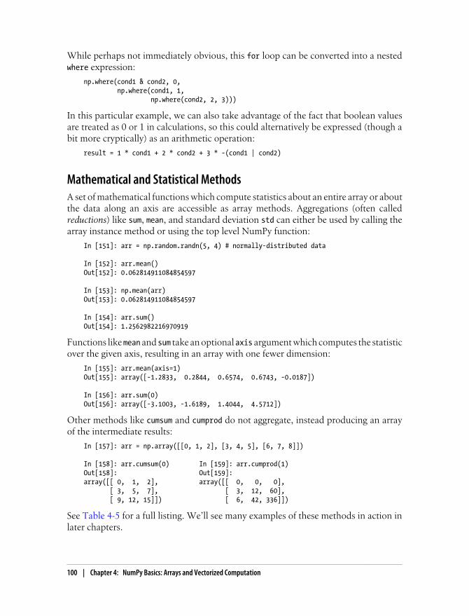
While perhaps not immediately obvious, this for loop can be converted into a nestedwhere expression:
np.where(cond1 & cond2, 0, np.where(cond1, 1, np.where(cond2, 2, 3)))
In this particular example, we can also take advantage of the fact that boolean valuesare treated as 0 or 1 in calculations, so this could alternatively be expressed (though abit more cryptically) as an arithmetic operation:
result = 1 * cond1 + 2 * cond2 + 3 * -(cond1 | cond2)
Mathematical and Statistical MethodsA set of mathematical functions which compute statistics about an entire array or aboutthe data along an axis are accessible as array methods. Aggregations (often calledreductions) like sum, mean, and standard deviation std can either be used by calling thearray instance method or using the top level NumPy function:
In [151]: arr = np.random.randn(5, 4) # normally-distributed data
In [152]: arr.mean()Out[152]: 0.062814911084854597
In [153]: np.mean(arr)Out[153]: 0.062814911084854597
In [154]: arr.sum()Out[154]: 1.2562982216970919
Functions like mean and sum take an optional axis argument which computes the statisticover the given axis, resulting in an array with one fewer dimension:
In [155]: arr.mean(axis=1)Out[155]: array([-1.2833, 0.2844, 0.6574, 0.6743, -0.0187])
In [156]: arr.sum(0)Out[156]: array([-3.1003, -1.6189, 1.4044, 4.5712])
Other methods like cumsum and cumprod do not aggregate, instead producing an arrayof the intermediate results:
In [157]: arr = np.array([[0, 1, 2], [3, 4, 5], [6, 7, 8]])
In [158]: arr.cumsum(0) In [159]: arr.cumprod(1)Out[158]: Out[159]: array([[ 0, 1, 2], array([[ 0, 0, 0], [ 3, 5, 7], [ 3, 12, 60], [ 9, 12, 15]]) [ 6, 42, 336]])
See Table 4-5 for a full listing. We’ll see many examples of these methods in action inlater chapters.
100 | Chapter 4: NumPy Basics: Arrays and Vectorized Computation

Table 4-5. Basic array statistical methods
Method Description
sum Sum of all the elements in the array or along an axis. Zero-length arrays have sum 0.
mean Arithmetic mean. Zero-length arrays have NaN mean.
std, var Standard deviation and variance, respectively, with optional degrees of freedom adjust-ment (default denominator n).
min, max Minimum and maximum.
argmin, argmax Indices of minimum and maximum elements, respectively.
cumsum Cumulative sum of elements starting from 0
cumprod Cumulative product of elements starting from 1
Methods for Boolean ArraysBoolean values are coerced to 1 (True) and 0 (False) in the above methods. Thus, sumis often used as a means of counting True values in a boolean array:
In [160]: arr = randn(100)
In [161]: (arr > 0).sum() # Number of positive valuesOut[161]: 44
There are two additional methods, any and all, useful especially for boolean arrays. any tests whether one or more values in an array is True, while all checks if every valueis True:
In [162]: bools = np.array([False, False, True, False])
In [163]: bools.any()Out[163]: True
In [164]: bools.all()Out[164]: False
These methods also work with non-boolean arrays, where non-zero elements evaluateto True.
SortingLike Python’s built-in list type, NumPy arrays can be sorted in-place using the sortmethod:
In [165]: arr = randn(8)
In [166]: arrOut[166]: array([ 0.6903, 0.4678, 0.0968, -0.1349, 0.9879, 0.0185, -1.3147, -0.5425])
In [167]: arr.sort()
Data Processing Using Arrays | 101
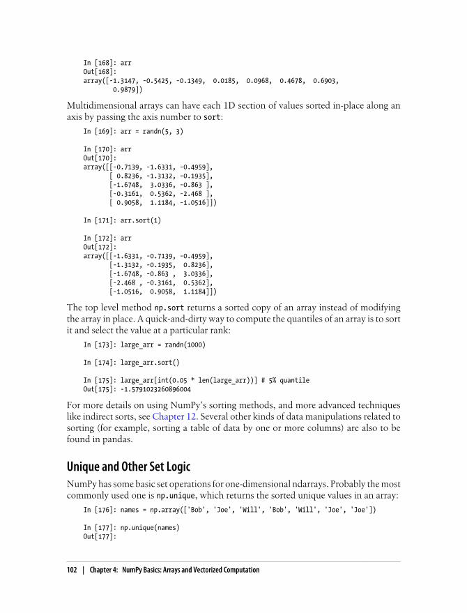
In [168]: arrOut[168]: array([-1.3147, -0.5425, -0.1349, 0.0185, 0.0968, 0.4678, 0.6903, 0.9879])
Multidimensional arrays can have each 1D section of values sorted in-place along anaxis by passing the axis number to sort:
In [169]: arr = randn(5, 3)
In [170]: arrOut[170]: array([[-0.7139, -1.6331, -0.4959], [ 0.8236, -1.3132, -0.1935], [-1.6748, 3.0336, -0.863 ], [-0.3161, 0.5362, -2.468 ], [ 0.9058, 1.1184, -1.0516]])
In [171]: arr.sort(1)
In [172]: arrOut[172]: array([[-1.6331, -0.7139, -0.4959], [-1.3132, -0.1935, 0.8236], [-1.6748, -0.863 , 3.0336], [-2.468 , -0.3161, 0.5362], [-1.0516, 0.9058, 1.1184]])
The top level method np.sort returns a sorted copy of an array instead of modifyingthe array in place. A quick-and-dirty way to compute the quantiles of an array is to sortit and select the value at a particular rank:
In [173]: large_arr = randn(1000)
In [174]: large_arr.sort()
In [175]: large_arr[int(0.05 * len(large_arr))] # 5% quantileOut[175]: -1.5791023260896004
For more details on using NumPy’s sorting methods, and more advanced techniqueslike indirect sorts, see Chapter 12. Several other kinds of data manipulations related tosorting (for example, sorting a table of data by one or more columns) are also to befound in pandas.
Unique and Other Set LogicNumPy has some basic set operations for one-dimensional ndarrays. Probably the mostcommonly used one is np.unique, which returns the sorted unique values in an array:
In [176]: names = np.array(['Bob', 'Joe', 'Will', 'Bob', 'Will', 'Joe', 'Joe'])
In [177]: np.unique(names)Out[177]:
102 | Chapter 4: NumPy Basics: Arrays and Vectorized Computation

array(['Bob', 'Joe', 'Will'], dtype='|S4')
In [178]: ints = np.array([3, 3, 3, 2, 2, 1, 1, 4, 4])
In [179]: np.unique(ints)Out[179]: array([1, 2, 3, 4])
Contrast np.unique with the pure Python alternative:
In [180]: sorted(set(names))Out[180]: ['Bob', 'Joe', 'Will']
Another function, np.in1d, tests membership of the values in one array in another,returning a boolean array:
In [181]: values = np.array([6, 0, 0, 3, 2, 5, 6])
In [182]: np.in1d(values, [2, 3, 6])Out[182]: array([ True, False, False, True, True, False, True], dtype=bool)
See Table 4-6 for a listing of set functions in NumPy.
Table 4-6. Array set operations
Method Description
unique(x) Compute the sorted, unique elements in x
intersect1d(x, y) Compute the sorted, common elements in x and y
union1d(x, y) Compute the sorted union of elements
in1d(x, y) Compute a boolean array indicating whether each element of x is contained in y
setdiff1d(x, y) Set difference, elements in x that are not in y
setxor1d(x, y) Set symmetric differences; elements that are in either of the arrays, but not both
File Input and Output with ArraysNumPy is able to save and load data to and from disk either in text or binary format.In later chapters you will learn about tools in pandas for reading tabular data intomemory.
Storing Arrays on Disk in Binary Formatnp.save and np.load are the two workhorse functions for efficiently saving and loadingarray data on disk. Arrays are saved by default in an uncompressed raw binary formatwith file extension .npy.
In [183]: arr = np.arange(10)
In [184]: np.save('some_array', arr)
File Input and Output with Arrays | 103

If the file path does not already end in .npy, the extension will be appended. The arrayon disk can then be loaded using np.load:
In [185]: np.load('some_array.npy')Out[185]: array([0, 1, 2, 3, 4, 5, 6, 7, 8, 9])
You save multiple arrays in a zip archive using np.savez and passing the arrays as key-word arguments:
In [186]: np.savez('array_archive.npz', a=arr, b=arr)
When loading an .npz file, you get back a dict-like object which loads the individualarrays lazily:
In [187]: arch = np.load('array_archive.npz')
In [188]: arch['b']Out[188]: array([0, 1, 2, 3, 4, 5, 6, 7, 8, 9])
Saving and Loading Text FilesLoading text from files is a fairly standard task. The landscape of file reading and writingfunctions in Python can be a bit confusing for a newcomer, so I will focus mainly onthe read_csv and read_table functions in pandas. It will at times be useful to load datainto vanilla NumPy arrays using np.loadtxt or the more specialized np.genfromtxt.
These functions have many options allowing you to specify different delimiters, con-verter functions for certain columns, skipping rows, and other things. Take a simplecase of a comma-separated file (CSV) like this:
In [191]: !cat array_ex.txt0.580052,0.186730,1.040717,1.1344110.194163,-0.636917,-0.938659,0.124094-0.126410,0.268607,-0.695724,0.047428-1.484413,0.004176,-0.744203,0.0054872.302869,0.200131,1.670238,-1.881090-0.193230,1.047233,0.482803,0.960334
This can be loaded into a 2D array like so:
In [192]: arr = np.loadtxt('array_ex.txt', delimiter=',')
In [193]: arrOut[193]: array([[ 0.5801, 0.1867, 1.0407, 1.1344], [ 0.1942, -0.6369, -0.9387, 0.1241], [-0.1264, 0.2686, -0.6957, 0.0474], [-1.4844, 0.0042, -0.7442, 0.0055], [ 2.3029, 0.2001, 1.6702, -1.8811], [-0.1932, 1.0472, 0.4828, 0.9603]])
np.savetxt performs the inverse operation: writing an array to a delimited text file.genfromtxt is similar to loadtxt but is geared for structured arrays and missing datahandling; see Chapter 12 for more on structured arrays.
104 | Chapter 4: NumPy Basics: Arrays and Vectorized Computation

For more on file reading and writing, especially tabular or spreadsheet-like data, see the later chapters involving pandas and DataFrame objects.
Linear AlgebraLinear algebra, like matrix multiplication, decompositions, determinants, and othersquare matrix math, is an important part of any array library. Unlike some languageslike MATLAB, multiplying two two-dimensional arrays with * is an element-wiseproduct instead of a matrix dot product. As such, there is a function dot, both an arraymethod, and a function in the numpy namespace, for matrix multiplication:
In [194]: x = np.array([[1., 2., 3.], [4., 5., 6.]])
In [195]: y = np.array([[6., 23.], [-1, 7], [8, 9]])
In [196]: x In [197]: y Out[196]: Out[197]: array([[ 1., 2., 3.], array([[ 6., 23.], [ 4., 5., 6.]]) [ -1., 7.], [ 8., 9.]]) In [198]: x.dot(y) # equivalently np.dot(x, y)Out[198]: array([[ 28., 64.], [ 67., 181.]])
A matrix product between a 2D array and a suitably sized 1D array results in a 1D array:
In [199]: np.dot(x, np.ones(3))Out[199]: array([ 6., 15.])
numpy.linalg has a standard set of matrix decompositions and things like inverse anddeterminant. These are implemented under the hood using the same industry-standardFortran libraries used in other languages like MATLAB and R, such as like BLAS, LA-PACK, or possibly (depending on your NumPy build) the Intel MKL:
In [201]: from numpy.linalg import inv, qr
In [202]: X = randn(5, 5)
In [203]: mat = X.T.dot(X)
In [204]: inv(mat)Out[204]: array([[ 3.0361, -0.1808, -0.6878, -2.8285, -1.1911], [-0.1808, 0.5035, 0.1215, 0.6702, 0.0956], [-0.6878, 0.1215, 0.2904, 0.8081, 0.3049], [-2.8285, 0.6702, 0.8081, 3.4152, 1.1557], [-1.1911, 0.0956, 0.3049, 1.1557, 0.6051]])
In [205]: mat.dot(inv(mat))
Linear Algebra | 105

Out[205]: array([[ 1., 0., 0., 0., -0.], [ 0., 1., -0., 0., 0.], [ 0., -0., 1., 0., 0.], [ 0., -0., -0., 1., -0.], [ 0., 0., 0., 0., 1.]])
In [206]: q, r = qr(mat)
In [207]: rOut[207]: array([[ -6.9271, 7.389 , 6.1227, -7.1163, -4.9215], [ 0. , -3.9735, -0.8671, 2.9747, -5.7402], [ 0. , 0. , -10.2681, 1.8909, 1.6079], [ 0. , 0. , 0. , -1.2996, 3.3577], [ 0. , 0. , 0. , 0. , 0.5571]])
See Table 4-7 for a list of some of the most commonly-used linear algebra functions.
The scientific Python community is hopeful that there may be a matrixmultiplication infix operator implemented someday, providing syntac-tically nicer alternative to using np.dot. But for now this is the way.
Table 4-7. Commonly-used numpy.linalg functions
Function Description
diag Return the diagonal (or off-diagonal) elements of a square matrix as a 1D array, or convert a 1D array into a squarematrix with zeros on the off-diagonal
dot Matrix multiplication
trace Compute the sum of the diagonal elements
det Compute the matrix determinant
eig Compute the eigenvalues and eigenvectors of a square matrix
inv Compute the inverse of a square matrix
pinv Compute the Moore-Penrose pseudo-inverse inverse of a square matrix
qr Compute the QR decomposition
svd Compute the singular value decomposition (SVD)
solve Solve the linear system Ax = b for x, where A is a square matrix
lstsq Compute the least-squares solution to y = Xb
Random Number GenerationThe numpy.random module supplements the built-in Python random with functions forefficiently generating whole arrays of sample values from many kinds of probability
106 | Chapter 4: NumPy Basics: Arrays and Vectorized Computation

distributions. For example, you can get a 4 by 4 array of samples from the standardnormal distribution using normal:
In [208]: samples = np.random.normal(size=(4, 4))
In [209]: samplesOut[209]: array([[ 0.1241, 0.3026, 0.5238, 0.0009], [ 1.3438, -0.7135, -0.8312, -2.3702], [-1.8608, -0.8608, 0.5601, -1.2659], [ 0.1198, -1.0635, 0.3329, -2.3594]])
Python’s built-in random module, by contrast, only samples one value at a time. As youcan see from this benchmark, numpy.random is well over an order of magnitude fasterfor generating very large samples:
In [210]: from random import normalvariate
In [211]: N = 1000000
In [212]: %timeit samples = [normalvariate(0, 1) for _ in xrange(N)]1 loops, best of 3: 1.33 s per loop
In [213]: %timeit np.random.normal(size=N)10 loops, best of 3: 57.7 ms per loop
See table Table 4-8 for a partial list of functions available in numpy.random. I’ll give someexamples of leveraging these functions’ ability to generate large arrays of samples all atonce in the next section.
Table 4-8. Partial list of numpy.random functions
Function Description
seed Seed the random number generator
permutation Return a random permutation of a sequence, or return a permuted range
shuffle Randomly permute a sequence in place
rand Draw samples from a uniform distribution
randint Draw random integers from a given low-to-high range
randn Draw samples from a normal distribution with mean 0 and standard deviation 1 (MATLAB-like interface)
binomial Draw samples a binomial distribution
normal Draw samples from a normal (Gaussian) distribution
beta Draw samples from a beta distribution
chisquare Draw samples from a chi-square distribution
gamma Draw samples from a gamma distribution
uniform Draw samples from a uniform [0, 1) distribution
Random Number Generation | 107
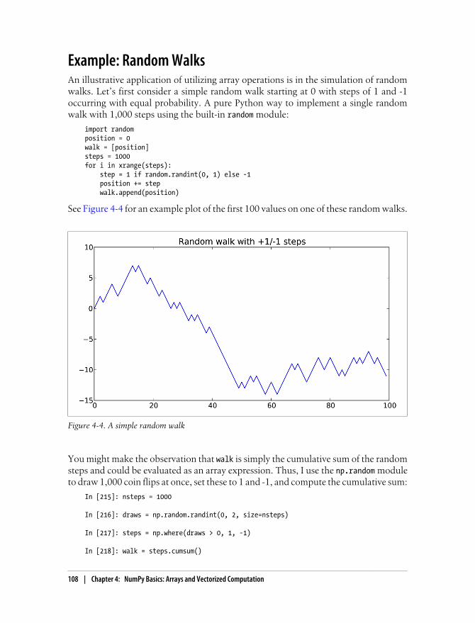
Example: Random WalksAn illustrative application of utilizing array operations is in the simulation of randomwalks. Let’s first consider a simple random walk starting at 0 with steps of 1 and -1occurring with equal probability. A pure Python way to implement a single randomwalk with 1,000 steps using the built-in random module:
import randomposition = 0walk = [position]steps = 1000for i in xrange(steps): step = 1 if random.randint(0, 1) else -1 position += step walk.append(position)
See Figure 4-4 for an example plot of the first 100 values on one of these random walks.
Figure 4-4. A simple random walk
You might make the observation that walk is simply the cumulative sum of the randomsteps and could be evaluated as an array expression. Thus, I use the np.random moduleto draw 1,000 coin flips at once, set these to 1 and -1, and compute the cumulative sum:
In [215]: nsteps = 1000
In [216]: draws = np.random.randint(0, 2, size=nsteps)
In [217]: steps = np.where(draws > 0, 1, -1)
In [218]: walk = steps.cumsum()
108 | Chapter 4: NumPy Basics: Arrays and Vectorized Computation

From this we can begin to extract statistics like the minimum and maximum value alongthe walk’s trajectory:
In [219]: walk.min() In [220]: walk.max()Out[219]: -3 Out[220]: 31
A more complicated statistic is the first crossing time, the step at which the randomwalk reaches a particular value. Here we might want to know how long it took therandom walk to get at least 10 steps away from the origin 0 in either direction.np.abs(walk) >= 10 gives us a boolean array indicating where the walk has reached orexceeded 10, but we want the index of the first 10 or -10. Turns out this can be com-puted using argmax, which returns the first index of the maximum value in the booleanarray (True is the maximum value):
In [221]: (np.abs(walk) >= 10).argmax()Out[221]: 37
Note that using argmax here is not always efficient because it always makes a full scanof the array. In this special case once a True is observed we know it to be the maximumvalue.
Simulating Many Random Walks at OnceIf your goal was to simulate many random walks, say 5,000 of them, you can generateall of the random walks with minor modifications to the above code. The numpy.random functions if passed a 2-tuple will generate a 2D array of draws, and we can computethe cumulative sum across the rows to compute all 5,000 random walks in one shot:
In [222]: nwalks = 5000
In [223]: nsteps = 1000
In [224]: draws = np.random.randint(0, 2, size=(nwalks, nsteps)) # 0 or 1
In [225]: steps = np.where(draws > 0, 1, -1)
In [226]: walks = steps.cumsum(1)
In [227]: walksOut[227]: array([[ 1, 0, 1, ..., 8, 7, 8], [ 1, 0, -1, ..., 34, 33, 32], [ 1, 0, -1, ..., 4, 5, 4], ..., [ 1, 2, 1, ..., 24, 25, 26], [ 1, 2, 3, ..., 14, 13, 14], [ -1, -2, -3, ..., -24, -23, -22]])
Now, we can compute the maximum and minimum values obtained over all of thewalks:
In [228]: walks.max() In [229]: walks.min()Out[228]: 138 Out[229]: -133
Example: Random Walks | 109

Out of these walks, let’s compute the minimum crossing time to 30 or -30. This isslightly tricky because not all 5,000 of them reach 30. We can check this using the any method:
In [230]: hits30 = (np.abs(walks) >= 30).any(1)
In [231]: hits30Out[231]: array([False, True, False, ..., False, True, False], dtype=bool)
In [232]: hits30.sum() # Number that hit 30 or -30Out[232]: 3410
We can use this boolean array to select out the rows of walks that actually cross theabsolute 30 level and call argmax across axis 1 to get the crossing times:
In [233]: crossing_times = (np.abs(walks[hits30]) >= 30).argmax(1)
In [234]: crossing_times.mean()Out[234]: 498.88973607038122
Feel free to experiment with other distributions for the steps other than equal sizedcoin flips. You need only use a different random number generation function, like normal to generate normally distributed steps with some mean and standard deviation:
In [235]: steps = np.random.normal(loc=0, scale=0.25, .....: size=(nwalks, nsteps))
110 | Chapter 4: NumPy Basics: Arrays and Vectorized Computation
CHAPTER 5
Getting Started with pandas
pandas will be the primary library of interest throughout much of the rest of the book.It contains high-level data structures and manipulation tools designed to make dataanalysis fast and easy in Python. pandas is built on top of NumPy and makes it easy touse in NumPy-centric applications.
As a bit of background, I started building pandas in early 2008 during my tenure atAQR, a quantitative investment management firm. At the time, I had a distinct set ofrequirements that were not well-addressed by any single tool at my disposal:
• Data structures with labeled axes supporting automatic or explicit data alignment.This prevents common errors resulting from misaligned data and working withdifferently-indexed data coming from different sources.
• Integrated time series functionality.
• The same data structures handle both time series data and non-time series data.
• Arithmetic operations and reductions (like summing across an axis) would passon the metadata (axis labels).
• Flexible handling of missing data.
• Merge and other relational operations found in popular database databases (SQL-based, for example).
I wanted to be able to do all of these things in one place, preferably in a language well-suited to general purpose software development. Python was a good candidate lan-guage for this, but at that time there was not an integrated set of data structures andtools providing this functionality.
Over the last four years, pandas has matured into a quite large library capable of solvinga much broader set of data handling problems than I ever anticipated, but it has ex-panded in its scope without compromising the simplicity and ease-of-use that I desiredfrom the very beginning. I hope that after reading this book, you will find it to be justas much of an indispensable tool as I do.
Throughout the rest of the book, I use the following import conventions for pandas:
111
In [1]: from pandas import Series, DataFrame
In [2]: import pandas as pd
Thus, whenever you see pd. in code, it’s referring to pandas. Series and DataFrame areused so much that I find it easier to import them into the local namespace.
Introduction to pandas Data StructuresTo get started with pandas, you will need to get comfortable with its two workhorsedata structures: Series and DataFrame. While they are not a universal solution for everyproblem, they provide a solid, easy-to-use basis for most applications.
SeriesA Series is a one-dimensional array-like object containing an array of data (of anyNumPy data type) and an associated array of data labels, called its index. The simplestSeries is formed from only an array of data:
In [4]: obj = Series([4, 7, -5, 3])
In [5]: objOut[5]: 0 41 72 -53 3
The string representation of a Series displayed interactively shows the index on the leftand the values on the right. Since we did not specify an index for the data, a defaultone consisting of the integers 0 through N - 1 (where N is the length of the data) iscreated. You can get the array representation and index object of the Series via its valuesand index attributes, respectively:
In [6]: obj.valuesOut[6]: array([ 4, 7, -5, 3])
In [7]: obj.indexOut[7]: Int64Index([0, 1, 2, 3])
Often it will be desirable to create a Series with an index identifying each data point:
In [8]: obj2 = Series([4, 7, -5, 3], index=['d', 'b', 'a', 'c'])
In [9]: obj2Out[9]: d 4b 7a -5c 3
112 | Chapter 5: Getting Started with pandas
In [10]: obj2.indexOut[10]: Index([d, b, a, c], dtype=object)
Compared with a regular NumPy array, you can use values in the index when selectingsingle values or a set of values:
In [11]: obj2['a']Out[11]: -5
In [12]: obj2['d'] = 6
In [13]: obj2[['c', 'a', 'd']]Out[13]: c 3a -5d 6
NumPy array operations, such as filtering with a boolean array, scalar multiplication,or applying math functions, will preserve the index-value link:
In [14]: obj2Out[14]: d 6b 7a -5c 3
In [15]: obj2[obj2 > 0] In [16]: obj2 * 2 In [17]: np.exp(obj2)Out[15]: Out[16]: Out[17]: d 6 d 12 d 403.428793 b 7 b 14 b 1096.633158 c 3 a -10 a 0.006738 c 6 c 20.085537
Another way to think about a Series is as a fixed-length, ordered dict, as it is a mappingof index values to data values. It can be substituted into many functions that expect adict:
In [18]: 'b' in obj2Out[18]: True
In [19]: 'e' in obj2Out[19]: False
Should you have data contained in a Python dict, you can create a Series from it bypassing the dict:
In [20]: sdata = {'Ohio': 35000, 'Texas': 71000, 'Oregon': 16000, 'Utah': 5000}
In [21]: obj3 = Series(sdata)
In [22]: obj3Out[22]: Ohio 35000Oregon 16000
Introduction to pandas Data Structures | 113

Texas 71000Utah 5000
When only passing a dict, the index in the resulting Series will have the dict’s keys insorted order.
In [23]: states = ['California', 'Ohio', 'Oregon', 'Texas']
In [24]: obj4 = Series(sdata, index=states)
In [25]: obj4Out[25]: California NaNOhio 35000Oregon 16000Texas 71000
In this case, 3 values found in sdata were placed in the appropriate locations, but sinceno value for 'California' was found, it appears as NaN (not a number) which is con-sidered in pandas to mark missing or NA values. I will use the terms “missing” or “NA”to refer to missing data. The isnull and notnull functions in pandas should be used todetect missing data:
In [26]: pd.isnull(obj4) In [27]: pd.notnull(obj4)Out[26]: Out[27]: California True California False Ohio False Ohio True Oregon False Oregon True Texas False Texas True
Series also has these as instance methods:
In [28]: obj4.isnull()Out[28]: California TrueOhio FalseOregon FalseTexas False
I discuss working with missing data in more detail later in this chapter.
A critical Series feature for many applications is that it automatically aligns differently-indexed data in arithmetic operations:
In [29]: obj3 In [30]: obj4 Out[29]: Out[30]: Ohio 35000 California NaNOregon 16000 Ohio 35000Texas 71000 Oregon 16000Utah 5000 Texas 71000 In [31]: obj3 + obj4Out[31]: California NaNOhio 70000Oregon 32000
114 | Chapter 5: Getting Started with pandas
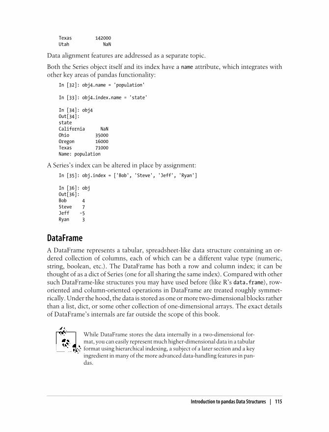
Texas 142000Utah NaN
Data alignment features are addressed as a separate topic.
Both the Series object itself and its index have a name attribute, which integrates withother key areas of pandas functionality:
In [32]: obj4.name = 'population'
In [33]: obj4.index.name = 'state'
In [34]: obj4Out[34]: stateCalifornia NaNOhio 35000Oregon 16000Texas 71000Name: population
A Series’s index can be altered in place by assignment:
In [35]: obj.index = ['Bob', 'Steve', 'Jeff', 'Ryan']
In [36]: objOut[36]: Bob 4Steve 7Jeff -5Ryan 3
DataFrameA DataFrame represents a tabular, spreadsheet-like data structure containing an or-dered collection of columns, each of which can be a different value type (numeric,string, boolean, etc.). The DataFrame has both a row and column index; it can bethought of as a dict of Series (one for all sharing the same index). Compared with othersuch DataFrame-like structures you may have used before (like R’s data.frame), row-oriented and column-oriented operations in DataFrame are treated roughly symmet-rically. Under the hood, the data is stored as one or more two-dimensional blocks ratherthan a list, dict, or some other collection of one-dimensional arrays. The exact detailsof DataFrame’s internals are far outside the scope of this book.
While DataFrame stores the data internally in a two-dimensional for-mat, you can easily represent much higher-dimensional data in a tabularformat using hierarchical indexing, a subject of a later section and a keyingredient in many of the more advanced data-handling features in pan-das.
Introduction to pandas Data Structures | 115

There are numerous ways to construct a DataFrame, though one of the most commonis from a dict of equal-length lists or NumPy arrays
data = {'state': ['Ohio', 'Ohio', 'Ohio', 'Nevada', 'Nevada'], 'year': [2000, 2001, 2002, 2001, 2002], 'pop': [1.5, 1.7, 3.6, 2.4, 2.9]}frame = DataFrame(data)
The resulting DataFrame will have its index assigned automatically as with Series, andthe columns are placed in sorted order:
In [38]: frameOut[38]: pop state year0 1.5 Ohio 20001 1.7 Ohio 20012 3.6 Ohio 20023 2.4 Nevada 20014 2.9 Nevada 2002
If you specify a sequence of columns, the DataFrame’s columns will be exactly whatyou pass:
In [39]: DataFrame(data, columns=['year', 'state', 'pop'])Out[39]: year state pop0 2000 Ohio 1.51 2001 Ohio 1.72 2002 Ohio 3.63 2001 Nevada 2.44 2002 Nevada 2.9
As with Series, if you pass a column that isn’t contained in data, it will appear with NAvalues in the result:
In [40]: frame2 = DataFrame(data, columns=['year', 'state', 'pop', 'debt'], ....: index=['one', 'two', 'three', 'four', 'five'])
In [41]: frame2Out[41]: year state pop debtone 2000 Ohio 1.5 NaNtwo 2001 Ohio 1.7 NaNthree 2002 Ohio 3.6 NaNfour 2001 Nevada 2.4 NaNfive 2002 Nevada 2.9 NaN
In [42]: frame2.columnsOut[42]: Index([year, state, pop, debt], dtype=object)
A column in a DataFrame can be retrieved as a Series either by dict-like notation or byattribute:
In [43]: frame2['state'] In [44]: frame2.yearOut[43]: Out[44]: one Ohio one 2000
116 | Chapter 5: Getting Started with pandas

two Ohio two 2001 three Ohio three 2002 four Nevada four 2001 five Nevada five 2002 Name: state Name: year
Note that the returned Series have the same index as the DataFrame, and their nameattribute has been appropriately set.
Rows can also be retrieved by position or name by a couple of methods, such as theix indexing field (much more on this later):
In [45]: frame2.ix['three']Out[45]: year 2002state Ohiopop 3.6debt NaNName: three
Columns can be modified by assignment. For example, the empty 'debt' column couldbe assigned a scalar value or an array of values:
In [46]: frame2['debt'] = 16.5
In [47]: frame2Out[47]: year state pop debtone 2000 Ohio 1.5 16.5two 2001 Ohio 1.7 16.5three 2002 Ohio 3.6 16.5four 2001 Nevada 2.4 16.5five 2002 Nevada 2.9 16.5
In [48]: frame2['debt'] = np.arange(5.)
In [49]: frame2Out[49]: year state pop debtone 2000 Ohio 1.5 0two 2001 Ohio 1.7 1three 2002 Ohio 3.6 2four 2001 Nevada 2.4 3five 2002 Nevada 2.9 4
When assigning lists or arrays to a column, the value’s length must match the lengthof the DataFrame. If you assign a Series, it will be instead conformed exactly to theDataFrame’s index, inserting missing values in any holes:
In [50]: val = Series([-1.2, -1.5, -1.7], index=['two', 'four', 'five'])
In [51]: frame2['debt'] = val
In [52]: frame2Out[52]: year state pop debt
Introduction to pandas Data Structures | 117

one 2000 Ohio 1.5 NaNtwo 2001 Ohio 1.7 -1.2three 2002 Ohio 3.6 NaNfour 2001 Nevada 2.4 -1.5five 2002 Nevada 2.9 -1.7
Assigning a column that doesn’t exist will create a new column. The del keyword willdelete columns as with a dict:
In [53]: frame2['eastern'] = frame2.state == 'Ohio'
In [54]: frame2Out[54]: year state pop debt easternone 2000 Ohio 1.5 NaN Truetwo 2001 Ohio 1.7 -1.2 Truethree 2002 Ohio 3.6 NaN Truefour 2001 Nevada 2.4 -1.5 Falsefive 2002 Nevada 2.9 -1.7 False
In [55]: del frame2['eastern']
In [56]: frame2.columnsOut[56]: Index([year, state, pop, debt], dtype=object)
The column returned when indexing a DataFrame is a view on the un-derlying data, not a copy. Thus, any in-place modifications to the Serieswill be reflected in the DataFrame. The column can be explicitly copiedusing the Series’s copy method.
Another common form of data is a nested dict of dicts format:
In [57]: pop = {'Nevada': {2001: 2.4, 2002: 2.9}, ....: 'Ohio': {2000: 1.5, 2001: 1.7, 2002: 3.6}}
If passed to DataFrame, it will interpret the outer dict keys as the columns and the innerkeys as the row indices:
In [58]: frame3 = DataFrame(pop)
In [59]: frame3Out[59]: Nevada Ohio2000 NaN 1.52001 2.4 1.72002 2.9 3.6
Of course you can always transpose the result:
In [60]: frame3.TOut[60]: 2000 2001 2002Nevada NaN 2.4 2.9Ohio 1.5 1.7 3.6
118 | Chapter 5: Getting Started with pandas

The keys in the inner dicts are unioned and sorted to form the index in the result. Thisisn’t true if an explicit index is specified:
In [61]: DataFrame(pop, index=[2001, 2002, 2003])Out[61]: Nevada Ohio2001 2.4 1.72002 2.9 3.62003 NaN NaN
Dicts of Series are treated much in the same way:
In [62]: pdata = {'Ohio': frame3['Ohio'][:-1], ....: 'Nevada': frame3['Nevada'][:2]}
In [63]: DataFrame(pdata)Out[63]: Nevada Ohio2000 NaN 1.52001 2.4 1.7
For a complete list of things you can pass the DataFrame constructor, see Table 5-1.
If a DataFrame’s index and columns have their name attributes set, these will also bedisplayed:
In [64]: frame3.index.name = 'year'; frame3.columns.name = 'state'
In [65]: frame3Out[65]: state Nevada Ohioyear 2000 NaN 1.52001 2.4 1.72002 2.9 3.6
Like Series, the values attribute returns the data contained in the DataFrame as a 2Dndarray:
In [66]: frame3.valuesOut[66]: array([[ nan, 1.5], [ 2.4, 1.7], [ 2.9, 3.6]])
If the DataFrame’s columns are different dtypes, the dtype of the values array will bechosen to accomodate all of the columns:
In [67]: frame2.valuesOut[67]: array([[2000, Ohio, 1.5, nan], [2001, Ohio, 1.7, -1.2], [2002, Ohio, 3.6, nan], [2001, Nevada, 2.4, -1.5], [2002, Nevada, 2.9, -1.7]], dtype=object)
Introduction to pandas Data Structures | 119
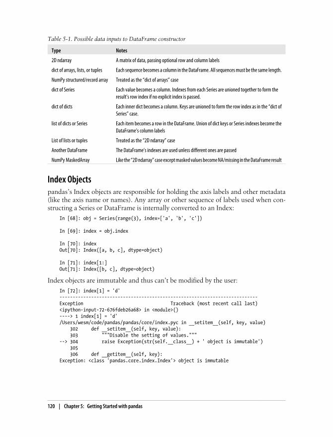
Table 5-1. Possible data inputs to DataFrame constructor
Type Notes
2D ndarray A matrix of data, passing optional row and column labels
dict of arrays, lists, or tuples Each sequence becomes a column in the DataFrame. All sequences must be the same length.
NumPy structured/record array Treated as the “dict of arrays” case
dict of Series Each value becomes a column. Indexes from each Series are unioned together to form theresult’s row index if no explicit index is passed.
dict of dicts Each inner dict becomes a column. Keys are unioned to form the row index as in the “dict ofSeries” case.
list of dicts or Series Each item becomes a row in the DataFrame. Union of dict keys or Series indexes become theDataFrame’s column labels
List of lists or tuples Treated as the “2D ndarray” case
Another DataFrame The DataFrame’s indexes are used unless different ones are passed
NumPy MaskedArray Like the “2D ndarray” case except masked values become NA/missing in the DataFrame result
Index Objectspandas’s Index objects are responsible for holding the axis labels and other metadata(like the axis name or names). Any array or other sequence of labels used when con-structing a Series or DataFrame is internally converted to an Index:
In [68]: obj = Series(range(3), index=['a', 'b', 'c'])
In [69]: index = obj.index
In [70]: indexOut[70]: Index([a, b, c], dtype=object)
In [71]: index[1:]Out[71]: Index([b, c], dtype=object)
Index objects are immutable and thus can’t be modified by the user:
In [72]: index[1] = 'd'---------------------------------------------------------------------------Exception Traceback (most recent call last)<ipython-input-72-676fdeb26a68> in <module>()----> 1 index[1] = 'd'/Users/wesm/code/pandas/pandas/core/index.pyc in __setitem__(self, key, value) 302 def __setitem__(self, key, value): 303 """Disable the setting of values."""--> 304 raise Exception(str(self.__class__) + ' object is immutable') 305 306 def __getitem__(self, key):Exception: <class 'pandas.core.index.Index'> object is immutable
120 | Chapter 5: Getting Started with pandas

Immutability is important so that Index objects can be safely shared among datastructures:
In [73]: index = pd.Index(np.arange(3))
In [74]: obj2 = Series([1.5, -2.5, 0], index=index)
In [75]: obj2.index is indexOut[75]: True
Table 5-2 has a list of built-in Index classes in the library. With some developmenteffort, Index can even be subclassed to implement specialized axis indexing function-ality.
Many users will not need to know much about Index objects, but they’renonetheless an important part of pandas’s data model.
Table 5-2. Main Index objects in pandas
Class Description
Index The most general Index object, representing axis labels in a NumPy array of Python objects.
Int64Index Specialized Index for integer values.
MultiIndex “Hierarchical” index object representing multiple levels of indexing on a single axis. Can be thought ofas similar to an array of tuples.
DatetimeIndex Stores nanosecond timestamps (represented using NumPy’s datetime64 dtype).
PeriodIndex Specialized Index for Period data (timespans).
In addition to being array-like, an Index also functions as a fixed-size set:
In [76]: frame3Out[76]: state Nevada Ohioyear 2000 NaN 1.52001 2.4 1.72002 2.9 3.6
In [77]: 'Ohio' in frame3.columnsOut[77]: True
In [78]: 2003 in frame3.indexOut[78]: False
Each Index has a number of methods and properties for set logic and answering othercommon questions about the data it contains. These are summarized in Table 5-3.
Introduction to pandas Data Structures | 121

Table 5-3. Index methods and properties
Method Description
append Concatenate with additional Index objects, producing a new Index
diff Compute set difference as an Index
intersection Compute set intersection
union Compute set union
isin Compute boolean array indicating whether each value is contained in the passed collection
delete Compute new Index with element at index i deleted
drop Compute new index by deleting passed values
insert Compute new Index by inserting element at index i
is_monotonic Returns True if each element is greater than or equal to the previous element
is_unique Returns True if the Index has no duplicate values
unique Compute the array of unique values in the Index
Essential FunctionalityIn this section, I’ll walk you through the fundamental mechanics of interacting withthe data contained in a Series or DataFrame. Upcoming chapters will delve more deeplyinto data analysis and manipulation topics using pandas. This book is not intended toserve as exhaustive documentation for the pandas library; I instead focus on the mostimportant features, leaving the less common (that is, more esoteric) things for you toexplore on your own.
ReindexingA critical method on pandas objects is reindex, which means to create a new objectwith the data conformed to a new index. Consider a simple example from above:
In [79]: obj = Series([4.5, 7.2, -5.3, 3.6], index=['d', 'b', 'a', 'c'])
In [80]: objOut[80]: d 4.5b 7.2a -5.3c 3.6
Calling reindex on this Series rearranges the data according to the new index, intro-ducing missing values if any index values were not already present:
In [81]: obj2 = obj.reindex(['a', 'b', 'c', 'd', 'e'])
In [82]: obj2Out[82]: a -5.3
122 | Chapter 5: Getting Started with pandas
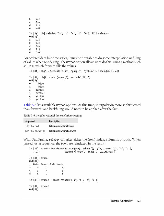
b 7.2c 3.6d 4.5e NaN
In [83]: obj.reindex(['a', 'b', 'c', 'd', 'e'], fill_value=0)Out[83]: a -5.3b 7.2c 3.6d 4.5e 0.0
For ordered data like time series, it may be desirable to do some interpolation or fillingof values when reindexing. The method option allows us to do this, using a method suchas ffill which forward fills the values:
In [84]: obj3 = Series(['blue', 'purple', 'yellow'], index=[0, 2, 4])
In [85]: obj3.reindex(range(6), method='ffill')Out[85]: 0 blue1 blue2 purple3 purple4 yellow5 yellow
Table 5-4 lists available method options. At this time, interpolation more sophisticatedthan forward- and backfilling would need to be applied after the fact.
Table 5-4. reindex method (interpolation) options
Argument Description
ffill or pad Fill (or carry) values forward
bfill or backfill Fill (or carry) values backward
With DataFrame, reindex can alter either the (row) index, columns, or both. Whenpassed just a sequence, the rows are reindexed in the result:
In [86]: frame = DataFrame(np.arange(9).reshape((3, 3)), index=['a', 'c', 'd'], ....: columns=['Ohio', 'Texas', 'California'])
In [87]: frameOut[87]: Ohio Texas Californiaa 0 1 2c 3 4 5d 6 7 8
In [88]: frame2 = frame.reindex(['a', 'b', 'c', 'd'])
In [89]: frame2Out[89]:
Essential Functionality | 123

Ohio Texas Californiaa 0 1 2b NaN NaN NaNc 3 4 5d 6 7 8
The columns can be reindexed using the columns keyword:
In [90]: states = ['Texas', 'Utah', 'California']
In [91]: frame.reindex(columns=states)Out[91]: Texas Utah Californiaa 1 NaN 2c 4 NaN 5d 7 NaN 8
Both can be reindexed in one shot, though interpolation will only apply row-wise (axis0):
In [92]: frame.reindex(index=['a', 'b', 'c', 'd'], method='ffill', ....: columns=states)Out[92]: Texas Utah Californiaa 1 NaN 2b 1 NaN 2c 4 NaN 5d 7 NaN 8
As you’ll see soon, reindexing can be done more succinctly by label-indexing with ix:
In [93]: frame.ix[['a', 'b', 'c', 'd'], states]Out[93]: Texas Utah Californiaa 1 NaN 2b NaN NaN NaNc 4 NaN 5d 7 NaN 8
Table 5-5. reindex function arguments
Argument Description
index New sequence to use as index. Can be Index instance or any other sequence-like Python data structure. AnIndex will be used exactly as is without any copying
method Interpolation (fill) method, see Table 5-4 for options.
fill_value Substitute value to use when introducing missing data by reindexing
limit When forward- or backfilling, maximum size gap to fill
level Match simple Index on level of MultiIndex, otherwise select subset of
copy Do not copy underlying data if new index is equivalent to old index. True by default (i.e. always copy data).
124 | Chapter 5: Getting Started with pandas

Dropping entries from an axisDropping one or more entries from an axis is easy if you have an index array or listwithout those entries. As that can require a bit of munging and set logic, the dropmethod will return a new object with the indicated value or values deleted from an axis:
In [94]: obj = Series(np.arange(5.), index=['a', 'b', 'c', 'd', 'e'])
In [95]: new_obj = obj.drop('c')
In [96]: new_objOut[96]: a 0b 1d 3e 4
In [97]: obj.drop(['d', 'c'])Out[97]: a 0b 1e 4
With DataFrame, index values can be deleted from either axis:
In [98]: data = DataFrame(np.arange(16).reshape((4, 4)), ....: index=['Ohio', 'Colorado', 'Utah', 'New York'], ....: columns=['one', 'two', 'three', 'four'])
In [99]: data.drop(['Colorado', 'Ohio'])Out[99]: one two three fourUtah 8 9 10 11New York 12 13 14 15
In [100]: data.drop('two', axis=1) In [101]: data.drop(['two', 'four'], axis=1)Out[100]: Out[101]: one three four one three Ohio 0 2 3 Ohio 0 2 Colorado 4 6 7 Colorado 4 6 Utah 8 10 11 Utah 8 10 New York 12 14 15 New York 12 14
Indexing, selection, and filteringSeries indexing (obj[...]) works analogously to NumPy array indexing, except you canuse the Series’s index values instead of only integers. Here are some examples this:
In [102]: obj = Series(np.arange(4.), index=['a', 'b', 'c', 'd'])
In [103]: obj['b'] In [104]: obj[1]Out[103]: 1.0 Out[104]: 1.0 In [105]: obj[2:4] In [106]: obj[['b', 'a', 'd']]Out[105]: Out[106]:
Essential Functionality | 125

c 2 b 1 d 3 a 0 d 3 In [107]: obj[[1, 3]] In [108]: obj[obj < 2]Out[107]: Out[108]: b 1 a 0 d 3 b 1
Slicing with labels behaves differently than normal Python slicing in that the endpointis inclusive:
In [109]: obj['b':'c']Out[109]: b 1c 2
Setting using these methods works just as you would expect:
In [110]: obj['b':'c'] = 5
In [111]: objOut[111]: a 0b 5c 5d 3
As you’ve seen above, indexing into a DataFrame is for retrieving one or more columnseither with a single value or sequence:
In [112]: data = DataFrame(np.arange(16).reshape((4, 4)), .....: index=['Ohio', 'Colorado', 'Utah', 'New York'], .....: columns=['one', 'two', 'three', 'four'])
In [113]: dataOut[113]: one two three fourOhio 0 1 2 3Colorado 4 5 6 7Utah 8 9 10 11New York 12 13 14 15
In [114]: data['two'] In [115]: data[['three', 'one']]Out[114]: Out[115]: Ohio 1 three one Colorado 5 Ohio 2 0 Utah 9 Colorado 6 4 New York 13 Utah 10 8 Name: two New York 14 12
Indexing like this has a few special cases. First selecting rows by slicing or a booleanarray:
In [116]: data[:2] In [117]: data[data['three'] > 5]Out[116]: Out[117]: one two three four one two three four
126 | Chapter 5: Getting Started with pandas
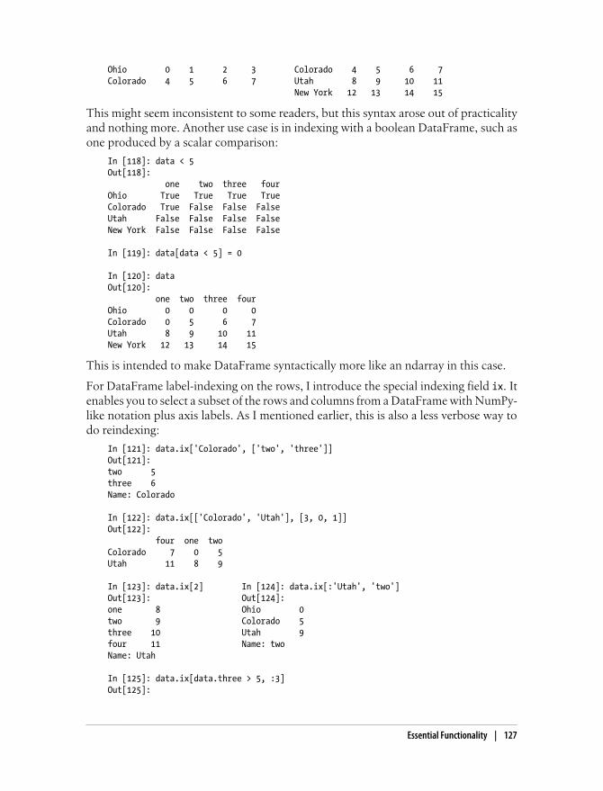
Ohio 0 1 2 3 Colorado 4 5 6 7 Colorado 4 5 6 7 Utah 8 9 10 11 New York 12 13 14 15
This might seem inconsistent to some readers, but this syntax arose out of practicalityand nothing more. Another use case is in indexing with a boolean DataFrame, such asone produced by a scalar comparison:
In [118]: data < 5Out[118]: one two three fourOhio True True True TrueColorado True False False FalseUtah False False False FalseNew York False False False False
In [119]: data[data < 5] = 0
In [120]: dataOut[120]: one two three fourOhio 0 0 0 0Colorado 0 5 6 7Utah 8 9 10 11New York 12 13 14 15
This is intended to make DataFrame syntactically more like an ndarray in this case.
For DataFrame label-indexing on the rows, I introduce the special indexing field ix. Itenables you to select a subset of the rows and columns from a DataFrame with NumPy-like notation plus axis labels. As I mentioned earlier, this is also a less verbose way todo reindexing:
In [121]: data.ix['Colorado', ['two', 'three']]Out[121]: two 5three 6Name: Colorado
In [122]: data.ix[['Colorado', 'Utah'], [3, 0, 1]]Out[122]: four one twoColorado 7 0 5Utah 11 8 9
In [123]: data.ix[2] In [124]: data.ix[:'Utah', 'two']Out[123]: Out[124]: one 8 Ohio 0 two 9 Colorado 5 three 10 Utah 9 four 11 Name: two Name: Utah In [125]: data.ix[data.three > 5, :3]Out[125]:
Essential Functionality | 127
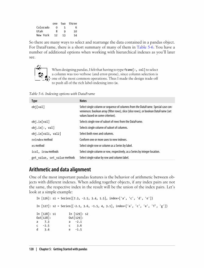
one two threeColorado 0 5 6Utah 8 9 10New York 12 13 14
So there are many ways to select and rearrange the data contained in a pandas object.For DataFrame, there is a short summary of many of them in Table 5-6. You have anumber of additional options when working with hierarchical indexes as you’ll latersee.
When designing pandas, I felt that having to type frame[:, col] to selecta column was too verbose (and error-prone), since column selection isone of the most common operations. Thus I made the design trade-offto push all of the rich label-indexing into ix.
Table 5-6. Indexing options with DataFrame
Type Notes
obj[val] Select single column or sequence of columns from the DataFrame. Special case con-veniences: boolean array (filter rows), slice (slice rows), or boolean DataFrame (setvalues based on some criterion).
obj.ix[val] Selects single row of subset of rows from the DataFrame.
obj.ix[:, val] Selects single column of subset of columns.
obj.ix[val1, val2] Select both rows and columns.
reindex method Conform one or more axes to new indexes.
xs method Select single row or column as a Series by label.
icol, irow methods Select single column or row, respectively, as a Series by integer location.
get_value, set_value methods Select single value by row and column label.
Arithmetic and data alignmentOne of the most important pandas features is the behavior of arithmetic between ob-jects with different indexes. When adding together objects, if any index pairs are notthe same, the respective index in the result will be the union of the index pairs. Let’slook at a simple example:
In [126]: s1 = Series([7.3, -2.5, 3.4, 1.5], index=['a', 'c', 'd', 'e'])
In [127]: s2 = Series([-2.1, 3.6, -1.5, 4, 3.1], index=['a', 'c', 'e', 'f', 'g'])
In [128]: s1 In [129]: s2Out[128]: Out[129]: a 7.3 a -2.1 c -2.5 c 3.6 d 3.4 e -1.5
128 | Chapter 5: Getting Started with pandas
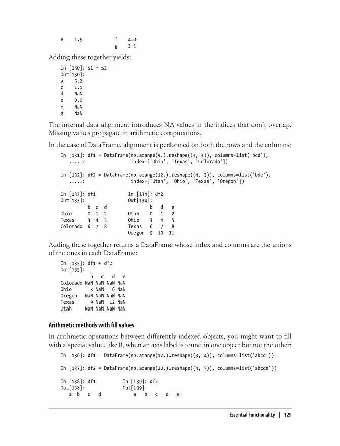
e 1.5 f 4.0 g 3.1
Adding these together yields:
In [130]: s1 + s2Out[130]: a 5.2c 1.1d NaNe 0.0f NaNg NaN
The internal data alignment introduces NA values in the indices that don’t overlap.Missing values propagate in arithmetic computations.
In the case of DataFrame, alignment is performed on both the rows and the columns:
In [131]: df1 = DataFrame(np.arange(9.).reshape((3, 3)), columns=list('bcd'), .....: index=['Ohio', 'Texas', 'Colorado'])
In [132]: df2 = DataFrame(np.arange(12.).reshape((4, 3)), columns=list('bde'), .....: index=['Utah', 'Ohio', 'Texas', 'Oregon'])
In [133]: df1 In [134]: df2 Out[133]: Out[134]: b c d b d eOhio 0 1 2 Utah 0 1 2Texas 3 4 5 Ohio 3 4 5Colorado 6 7 8 Texas 6 7 8 Oregon 9 10 11
Adding these together returns a DataFrame whose index and columns are the unionsof the ones in each DataFrame:
In [135]: df1 + df2Out[135]: b c d eColorado NaN NaN NaN NaNOhio 3 NaN 6 NaNOregon NaN NaN NaN NaNTexas 9 NaN 12 NaNUtah NaN NaN NaN NaN
Arithmetic methods with fill values
In arithmetic operations between differently-indexed objects, you might want to fillwith a special value, like 0, when an axis label is found in one object but not the other:
In [136]: df1 = DataFrame(np.arange(12.).reshape((3, 4)), columns=list('abcd'))
In [137]: df2 = DataFrame(np.arange(20.).reshape((4, 5)), columns=list('abcde'))
In [138]: df1 In [139]: df2 Out[138]: Out[139]: a b c d a b c d e
Essential Functionality | 129

0 0 1 2 3 0 0 1 2 3 41 4 5 6 7 1 5 6 7 8 92 8 9 10 11 2 10 11 12 13 14 3 15 16 17 18 19
Adding these together results in NA values in the locations that don’t overlap:
In [140]: df1 + df2Out[140]: a b c d e0 0 2 4 6 NaN1 9 11 13 15 NaN2 18 20 22 24 NaN3 NaN NaN NaN NaN NaN
Using the add method on df1, I pass df2 and an argument to fill_value:
In [141]: df1.add(df2, fill_value=0)Out[141]: a b c d e0 0 2 4 6 41 9 11 13 15 92 18 20 22 24 143 15 16 17 18 19
Relatedly, when reindexing a Series or DataFrame, you can also specify a different fillvalue:
In [142]: df1.reindex(columns=df2.columns, fill_value=0)Out[142]: a b c d e0 0 1 2 3 01 4 5 6 7 02 8 9 10 11 0
Table 5-7. Flexible arithmetic methods
Method Description
add Method for addition (+)
sub Method for subtraction (-)
div Method for division (/)
mul Method for multiplication (*)
Operations between DataFrame and Series
As with NumPy arrays, arithmetic between DataFrame and Series is well-defined. First,as a motivating example, consider the difference between a 2D array and one of its rows:
In [143]: arr = np.arange(12.).reshape((3, 4))
In [144]: arrOut[144]: array([[ 0., 1., 2., 3.], [ 4., 5., 6., 7.],
130 | Chapter 5: Getting Started with pandas
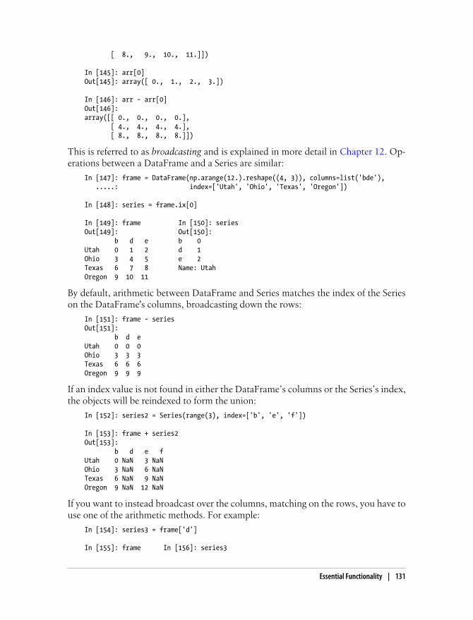
[ 8., 9., 10., 11.]])
In [145]: arr[0]Out[145]: array([ 0., 1., 2., 3.])
In [146]: arr - arr[0]Out[146]: array([[ 0., 0., 0., 0.], [ 4., 4., 4., 4.], [ 8., 8., 8., 8.]])
This is referred to as broadcasting and is explained in more detail in Chapter 12. Op-erations between a DataFrame and a Series are similar:
In [147]: frame = DataFrame(np.arange(12.).reshape((4, 3)), columns=list('bde'), .....: index=['Utah', 'Ohio', 'Texas', 'Oregon'])
In [148]: series = frame.ix[0]
In [149]: frame In [150]: seriesOut[149]: Out[150]: b d e b 0 Utah 0 1 2 d 1 Ohio 3 4 5 e 2 Texas 6 7 8 Name: Utah Oregon 9 10 11
By default, arithmetic between DataFrame and Series matches the index of the Serieson the DataFrame's columns, broadcasting down the rows:
In [151]: frame - seriesOut[151]: b d eUtah 0 0 0Ohio 3 3 3Texas 6 6 6Oregon 9 9 9
If an index value is not found in either the DataFrame’s columns or the Series’s index,the objects will be reindexed to form the union:
In [152]: series2 = Series(range(3), index=['b', 'e', 'f'])
In [153]: frame + series2Out[153]: b d e fUtah 0 NaN 3 NaNOhio 3 NaN 6 NaNTexas 6 NaN 9 NaNOregon 9 NaN 12 NaN
If you want to instead broadcast over the columns, matching on the rows, you have touse one of the arithmetic methods. For example:
In [154]: series3 = frame['d']
In [155]: frame In [156]: series3
Essential Functionality | 131
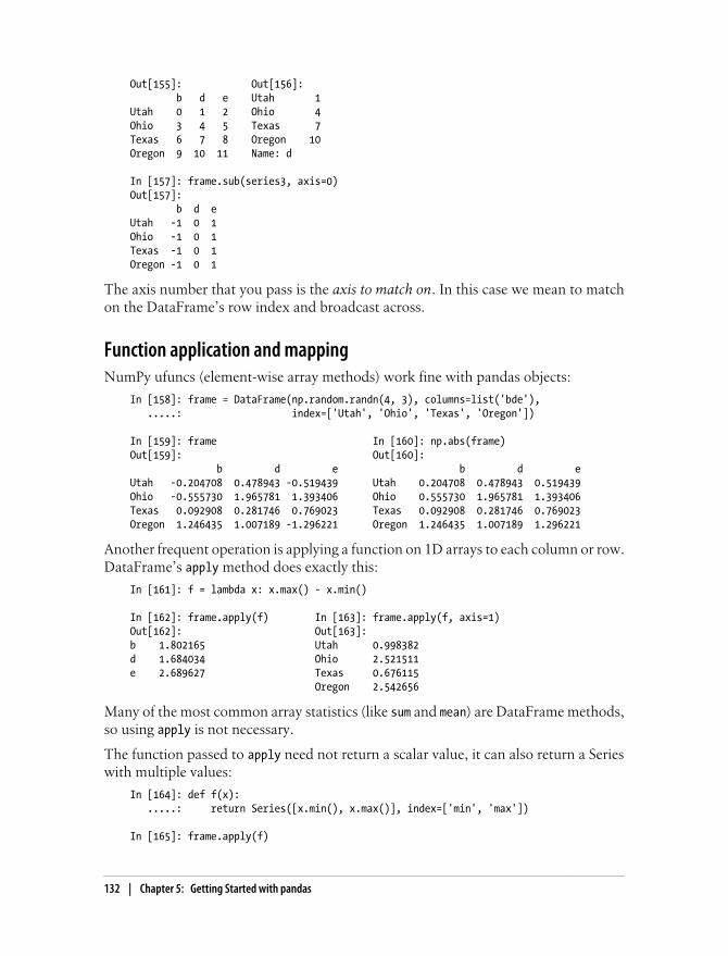
Out[155]: Out[156]: b d e Utah 1 Utah 0 1 2 Ohio 4 Ohio 3 4 5 Texas 7 Texas 6 7 8 Oregon 10 Oregon 9 10 11 Name: d In [157]: frame.sub(series3, axis=0)Out[157]: b d eUtah -1 0 1Ohio -1 0 1Texas -1 0 1Oregon -1 0 1
The axis number that you pass is the axis to match on. In this case we mean to matchon the DataFrame’s row index and broadcast across.
Function application and mappingNumPy ufuncs (element-wise array methods) work fine with pandas objects:
In [158]: frame = DataFrame(np.random.randn(4, 3), columns=list('bde'), .....: index=['Utah', 'Ohio', 'Texas', 'Oregon'])
In [159]: frame In [160]: np.abs(frame) Out[159]: Out[160]: b d e b d eUtah -0.204708 0.478943 -0.519439 Utah 0.204708 0.478943 0.519439Ohio -0.555730 1.965781 1.393406 Ohio 0.555730 1.965781 1.393406Texas 0.092908 0.281746 0.769023 Texas 0.092908 0.281746 0.769023Oregon 1.246435 1.007189 -1.296221 Oregon 1.246435 1.007189 1.296221
Another frequent operation is applying a function on 1D arrays to each column or row.DataFrame’s apply method does exactly this:
In [161]: f = lambda x: x.max() - x.min()
In [162]: frame.apply(f) In [163]: frame.apply(f, axis=1)Out[162]: Out[163]: b 1.802165 Utah 0.998382 d 1.684034 Ohio 2.521511 e 2.689627 Texas 0.676115 Oregon 2.542656
Many of the most common array statistics (like sum and mean) are DataFrame methods,so using apply is not necessary.
The function passed to apply need not return a scalar value, it can also return a Serieswith multiple values:
In [164]: def f(x): .....: return Series([x.min(), x.max()], index=['min', 'max'])
In [165]: frame.apply(f)
132 | Chapter 5: Getting Started with pandas
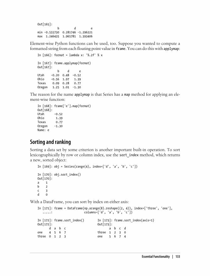
Out[165]: b d emin -0.555730 0.281746 -1.296221max 1.246435 1.965781 1.393406
Element-wise Python functions can be used, too. Suppose you wanted to compute aformatted string from each floating point value in frame. You can do this with applymap:
In [166]: format = lambda x: '%.2f' % x
In [167]: frame.applymap(format)Out[167]: b d eUtah -0.20 0.48 -0.52Ohio -0.56 1.97 1.39Texas 0.09 0.28 0.77Oregon 1.25 1.01 -1.30
The reason for the name applymap is that Series has a map method for applying an ele-ment-wise function:
In [168]: frame['e'].map(format)Out[168]: Utah -0.52Ohio 1.39Texas 0.77Oregon -1.30Name: e
Sorting and rankingSorting a data set by some criterion is another important built-in operation. To sortlexicographically by row or column index, use the sort_index method, which returnsa new, sorted object:
In [169]: obj = Series(range(4), index=['d', 'a', 'b', 'c'])
In [170]: obj.sort_index()Out[170]: a 1b 2c 3d 0
With a DataFrame, you can sort by index on either axis:
In [171]: frame = DataFrame(np.arange(8).reshape((2, 4)), index=['three', 'one'], .....: columns=['d', 'a', 'b', 'c'])
In [172]: frame.sort_index() In [173]: frame.sort_index(axis=1)Out[172]: Out[173]: d a b c a b c d one 4 5 6 7 three 1 2 3 0 three 0 1 2 3 one 5 6 7 4
Essential Functionality | 133

The data is sorted in ascending order by default, but can be sorted in descending order,too:
In [174]: frame.sort_index(axis=1, ascending=False)Out[174]: d c b athree 0 3 2 1one 4 7 6 5
To sort a Series by its values, use its order method:
In [175]: obj = Series([4, 7, -3, 2])
In [176]: obj.order()Out[176]: 2 -33 20 41 7
Any missing values are sorted to the end of the Series by default:
In [177]: obj = Series([4, np.nan, 7, np.nan, -3, 2])
In [178]: obj.order()Out[178]: 4 -35 20 42 71 NaN3 NaN
On DataFrame, you may want to sort by the values in one or more columns. To do so,pass one or more column names to the by option:
In [179]: frame = DataFrame({'b': [4, 7, -3, 2], 'a': [0, 1, 0, 1]})
In [180]: frame In [181]: frame.sort_index(by='b')Out[180]: Out[181]: a b a b 0 0 4 2 0 -3 1 1 7 3 1 2 2 0 -3 0 0 4 3 1 2 1 1 7
To sort by multiple columns, pass a list of names:
In [182]: frame.sort_index(by=['a', 'b'])Out[182]: a b2 0 -30 0 43 1 21 1 7
134 | Chapter 5: Getting Started with pandas
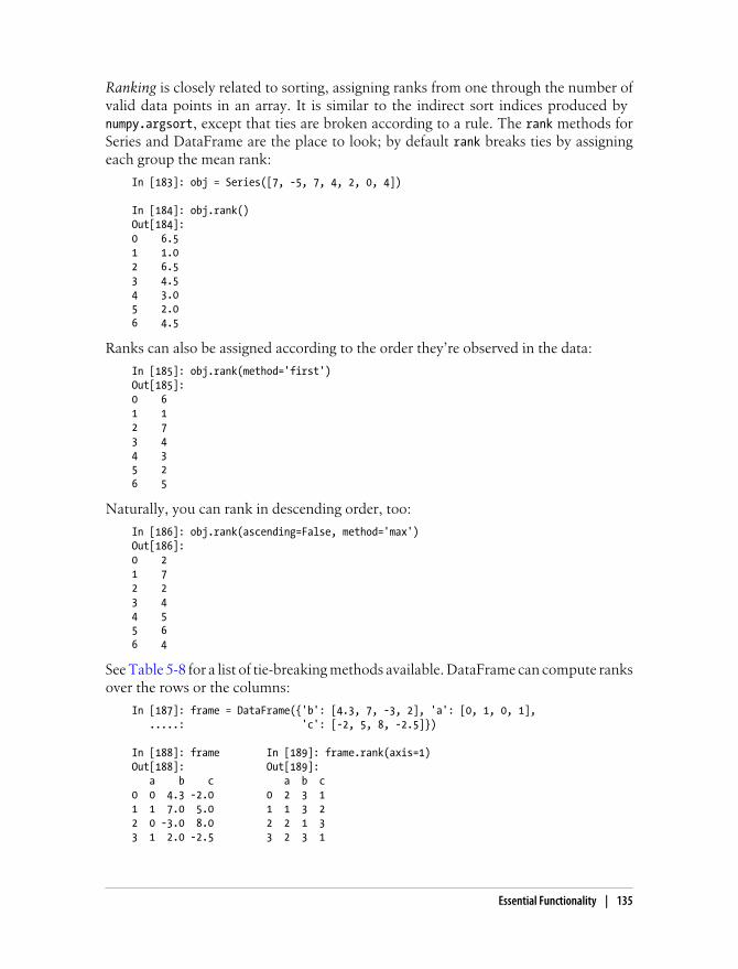
Ranking is closely related to sorting, assigning ranks from one through the number ofvalid data points in an array. It is similar to the indirect sort indices produced by numpy.argsort, except that ties are broken according to a rule. The rank methods forSeries and DataFrame are the place to look; by default rank breaks ties by assigningeach group the mean rank:
In [183]: obj = Series([7, -5, 7, 4, 2, 0, 4])
In [184]: obj.rank()Out[184]: 0 6.51 1.02 6.53 4.54 3.05 2.06 4.5
Ranks can also be assigned according to the order they’re observed in the data:
In [185]: obj.rank(method='first')Out[185]: 0 61 12 73 44 35 26 5
Naturally, you can rank in descending order, too:
In [186]: obj.rank(ascending=False, method='max')Out[186]: 0 21 72 23 44 55 66 4
See Table 5-8 for a list of tie-breaking methods available. DataFrame can compute ranksover the rows or the columns:
In [187]: frame = DataFrame({'b': [4.3, 7, -3, 2], 'a': [0, 1, 0, 1], .....: 'c': [-2, 5, 8, -2.5]})
In [188]: frame In [189]: frame.rank(axis=1)Out[188]: Out[189]: a b c a b c 0 0 4.3 -2.0 0 2 3 1 1 1 7.0 5.0 1 1 3 2 2 0 -3.0 8.0 2 2 1 3 3 1 2.0 -2.5 3 2 3 1
Essential Functionality | 135

Table 5-8. Tie-breaking methods with rank
Method Description
'average' Default: assign the average rank to each entry in the equal group.
'min' Use the minimum rank for the whole group.
'max' Use the maximum rank for the whole group.
'first' Assign ranks in the order the values appear in the data.
Axis indexes with duplicate valuesUp until now all of the examples I’ve showed you have had unique axis labels (indexvalues). While many pandas functions (like reindex) require that the labels be unique,it’s not mandatory. Let’s consider a small Series with duplicate indices:
In [190]: obj = Series(range(5), index=['a', 'a', 'b', 'b', 'c'])
In [191]: objOut[191]: a 0a 1b 2b 3c 4
The index’s is_unique property can tell you whether its values are unique or not:
In [192]: obj.index.is_uniqueOut[192]: False
Data selection is one of the main things that behaves differently with duplicates. In-dexing a value with multiple entries returns a Series while single entries return a scalarvalue:
In [193]: obj['a'] In [194]: obj['c']Out[193]: Out[194]: 4 a 0 a 1
The same logic extends to indexing rows in a DataFrame:
In [195]: df = DataFrame(np.random.randn(4, 3), index=['a', 'a', 'b', 'b'])
In [196]: dfOut[196]: 0 1 2a 0.274992 0.228913 1.352917a 0.886429 -2.001637 -0.371843b 1.669025 -0.438570 -0.539741b 0.476985 3.248944 -1.021228
In [197]: df.ix['b']Out[197]: 0 1 2
136 | Chapter 5: Getting Started with pandas

b 1.669025 -0.438570 -0.539741b 0.476985 3.248944 -1.021228
Summarizing and Computing Descriptive Statisticspandas objects are equipped with a set of common mathematical and statistical meth-ods. Most of these fall into the category of reductions or summary statistics, methodsthat extract a single value (like the sum or mean) from a Series or a Series of values fromthe rows or columns of a DataFrame. Compared with the equivalent methods of vanillaNumPy arrays, they are all built from the ground up to exclude missing data. Considera small DataFrame:
In [198]: df = DataFrame([[1.4, np.nan], [7.1, -4.5], .....: [np.nan, np.nan], [0.75, -1.3]], .....: index=['a', 'b', 'c', 'd'], .....: columns=['one', 'two'])
In [199]: dfOut[199]: one twoa 1.40 NaNb 7.10 -4.5c NaN NaNd 0.75 -1.3
Calling DataFrame’s sum method returns a Series containing column sums:
In [200]: df.sum()Out[200]: one 9.25two -5.80
Passing axis=1 sums over the rows instead:
In [201]: df.sum(axis=1)Out[201]: a 1.40b 2.60c NaNd -0.55
NA values are excluded unless the entire slice (row or column in this case) is NA. Thiscan be disabled using the skipna option:
In [202]: df.mean(axis=1, skipna=False)Out[202]: a NaNb 1.300c NaNd -0.275
See Table 5-9 for a list of common options for each reduction method options.
Summarizing and Computing Descriptive Statistics | 137

Table 5-9. Options for reduction methods
Method Description
axis Axis to reduce over. 0 for DataFrame’s rows and 1 for columns.
skipna Exclude missing values, True by default.
level Reduce grouped by level if the axis is hierarchically-indexed (MultiIndex).
Some methods, like idxmin and idxmax, return indirect statistics like the index valuewhere the minimum or maximum values are attained:
In [203]: df.idxmax()Out[203]: one btwo d
Other methods are accumulations:
In [204]: df.cumsum()Out[204]: one twoa 1.40 NaNb 8.50 -4.5c NaN NaNd 9.25 -5.8
Another type of method is neither a reduction nor an accumulation. describe is onesuch example, producing multiple summary statistics in one shot:
In [205]: df.describe()Out[205]: one twocount 3.000000 2.000000mean 3.083333 -2.900000std 3.493685 2.262742min 0.750000 -4.50000025% 1.075000 -3.70000050% 1.400000 -2.90000075% 4.250000 -2.100000max 7.100000 -1.300000
On non-numeric data, describe produces alternate summary statistics:
In [206]: obj = Series(['a', 'a', 'b', 'c'] * 4)
In [207]: obj.describe()Out[207]: count 16unique 3top afreq 8
See Table 5-10 for a full list of summary statistics and related methods.
138 | Chapter 5: Getting Started with pandas

Table 5-10. Descriptive and summary statistics
Method Description
count Number of non-NA values
describe Compute set of summary statistics for Series or each DataFrame column
min, max Compute minimum and maximum values
argmin, argmax Compute index locations (integers) at which minimum or maximum value obtained, respectively
idxmin, idxmax Compute index values at which minimum or maximum value obtained, respectively
quantile Compute sample quantile ranging from 0 to 1
sum Sum of values
mean Mean of values
median Arithmetic median (50% quantile) of values
mad Mean absolute deviation from mean value
var Sample variance of values
std Sample standard deviation of values
skew Sample skewness (3rd moment) of values
kurt Sample kurtosis (4th moment) of values
cumsum Cumulative sum of values
cummin, cummax Cumulative minimum or maximum of values, respectively
cumprod Cumulative product of values
diff Compute 1st arithmetic difference (useful for time series)
pct_change Compute percent changes
Correlation and CovarianceSome summary statistics, like correlation and covariance, are computed from pairs ofarguments. Let’s consider some DataFrames of stock prices and volumes obtained fromYahoo! Finance:
import pandas.io.data as web
all_data = {}for ticker in ['AAPL', 'IBM', 'MSFT', 'GOOG']: all_data[ticker] = web.get_data_yahoo(ticker, '1/1/2000', '1/1/2010')
price = DataFrame({tic: data['Adj Close'] for tic, data in all_data.iteritems()})volume = DataFrame({tic: data['Volume'] for tic, data in all_data.iteritems()})
I now compute percent changes of the prices:
In [209]: returns = price.pct_change()
In [210]: returns.tail()
Summarizing and Computing Descriptive Statistics | 139
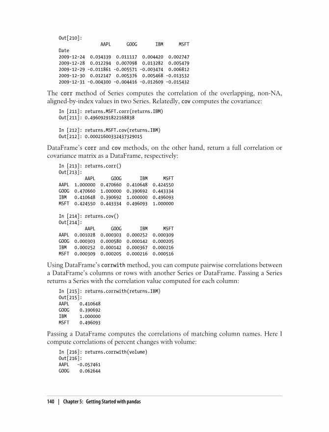
Out[210]: AAPL GOOG IBM MSFTDate 2009-12-24 0.034339 0.011117 0.004420 0.0027472009-12-28 0.012294 0.007098 0.013282 0.0054792009-12-29 -0.011861 -0.005571 -0.003474 0.0068122009-12-30 0.012147 0.005376 0.005468 -0.0135322009-12-31 -0.004300 -0.004416 -0.012609 -0.015432
The corr method of Series computes the correlation of the overlapping, non-NA,aligned-by-index values in two Series. Relatedly, cov computes the covariance:
In [211]: returns.MSFT.corr(returns.IBM)Out[211]: 0.49609291822168838
In [212]: returns.MSFT.cov(returns.IBM)Out[212]: 0.00021600332437329015
DataFrame’s corr and cov methods, on the other hand, return a full correlation orcovariance matrix as a DataFrame, respectively:
In [213]: returns.corr()Out[213]: AAPL GOOG IBM MSFTAAPL 1.000000 0.470660 0.410648 0.424550GOOG 0.470660 1.000000 0.390692 0.443334IBM 0.410648 0.390692 1.000000 0.496093MSFT 0.424550 0.443334 0.496093 1.000000
In [214]: returns.cov()Out[214]: AAPL GOOG IBM MSFTAAPL 0.001028 0.000303 0.000252 0.000309GOOG 0.000303 0.000580 0.000142 0.000205IBM 0.000252 0.000142 0.000367 0.000216MSFT 0.000309 0.000205 0.000216 0.000516
Using DataFrame’s corrwith method, you can compute pairwise correlations betweena DataFrame’s columns or rows with another Series or DataFrame. Passing a Seriesreturns a Series with the correlation value computed for each column:
In [215]: returns.corrwith(returns.IBM)Out[215]: AAPL 0.410648GOOG 0.390692IBM 1.000000MSFT 0.496093
Passing a DataFrame computes the correlations of matching column names. Here Icompute correlations of percent changes with volume:
In [216]: returns.corrwith(volume)Out[216]: AAPL -0.057461GOOG 0.062644
140 | Chapter 5: Getting Started with pandas
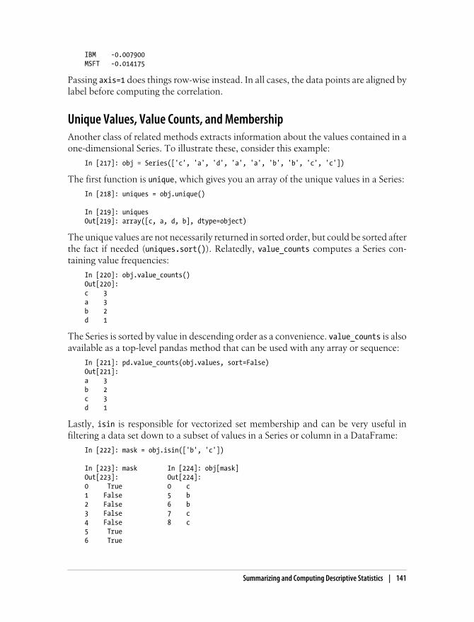
IBM -0.007900MSFT -0.014175
Passing axis=1 does things row-wise instead. In all cases, the data points are aligned bylabel before computing the correlation.
Unique Values, Value Counts, and MembershipAnother class of related methods extracts information about the values contained in aone-dimensional Series. To illustrate these, consider this example:
In [217]: obj = Series(['c', 'a', 'd', 'a', 'a', 'b', 'b', 'c', 'c'])
The first function is unique, which gives you an array of the unique values in a Series:
In [218]: uniques = obj.unique()
In [219]: uniquesOut[219]: array([c, a, d, b], dtype=object)
The unique values are not necessarily returned in sorted order, but could be sorted afterthe fact if needed (uniques.sort()). Relatedly, value_counts computes a Series con-taining value frequencies:
In [220]: obj.value_counts()Out[220]: c 3a 3b 2d 1
The Series is sorted by value in descending order as a convenience. value_counts is alsoavailable as a top-level pandas method that can be used with any array or sequence:
In [221]: pd.value_counts(obj.values, sort=False)Out[221]: a 3b 2c 3d 1
Lastly, isin is responsible for vectorized set membership and can be very useful infiltering a data set down to a subset of values in a Series or column in a DataFrame:
In [222]: mask = obj.isin(['b', 'c'])
In [223]: mask In [224]: obj[mask]Out[223]: Out[224]: 0 True 0 c 1 False 5 b 2 False 6 b 3 False 7 c 4 False 8 c 5 True 6 True
Summarizing and Computing Descriptive Statistics | 141
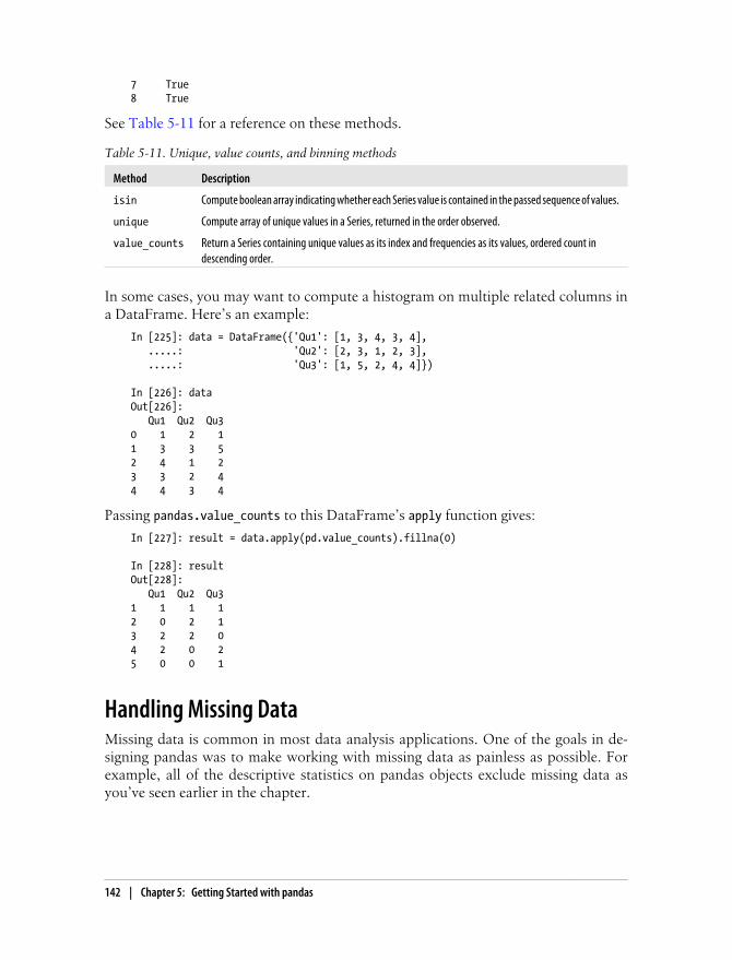
7 True 8 True
See Table 5-11 for a reference on these methods.
Table 5-11. Unique, value counts, and binning methods
Method Description
isin Compute boolean array indicating whether each Series value is contained in the passed sequence of values.
unique Compute array of unique values in a Series, returned in the order observed.
value_counts Return a Series containing unique values as its index and frequencies as its values, ordered count indescending order.
In some cases, you may want to compute a histogram on multiple related columns ina DataFrame. Here’s an example:
In [225]: data = DataFrame({'Qu1': [1, 3, 4, 3, 4], .....: 'Qu2': [2, 3, 1, 2, 3], .....: 'Qu3': [1, 5, 2, 4, 4]})
In [226]: dataOut[226]: Qu1 Qu2 Qu30 1 2 11 3 3 52 4 1 23 3 2 44 4 3 4
Passing pandas.value_counts to this DataFrame’s apply function gives:
In [227]: result = data.apply(pd.value_counts).fillna(0)
In [228]: resultOut[228]: Qu1 Qu2 Qu31 1 1 12 0 2 13 2 2 04 2 0 25 0 0 1
Handling Missing DataMissing data is common in most data analysis applications. One of the goals in de-signing pandas was to make working with missing data as painless as possible. Forexample, all of the descriptive statistics on pandas objects exclude missing data asyou’ve seen earlier in the chapter.
142 | Chapter 5: Getting Started with pandas

pandas uses the floating point value NaN (Not a Number) to represent missing data inboth floating as well as in non-floating point arrays. It is just used as a sentinel that canbe easily detected:
In [229]: string_data = Series(['aardvark', 'artichoke', np.nan, 'avocado'])
In [230]: string_data In [231]: string_data.isnull()Out[230]: Out[231]: 0 aardvark 0 False 1 artichoke 1 False 2 NaN 2 True 3 avocado 3 False
The built-in Python None value is also treated as NA in object arrays:
In [232]: string_data[0] = None
In [233]: string_data.isnull()Out[233]: 0 True1 False2 True3 False
I do not claim that pandas’s NA representation is optimal, but it is simple and reason-ably consistent. It’s the best solution, with good all-around performance characteristicsand a simple API, that I could concoct in the absence of a true NA data type or bitpattern in NumPy’s data types. Ongoing development work in NumPy may change thisin the future.
Table 5-12. NA handling methods
Argument Description
dropna Filter axis labels based on whether values for each label have missing data, with varying thresholds for how muchmissing data to tolerate.
fillna Fill in missing data with some value or using an interpolation method such as 'ffill' or 'bfill'.
isnull Return like-type object containing boolean values indicating which values are missing / NA.
notnull Negation of isnull.
Filtering Out Missing DataYou have a number of options for filtering out missing data. While doing it by hand isalways an option, dropna can be very helpful. On a Series, it returns the Series with onlythe non-null data and index values:
In [234]: from numpy import nan as NA
In [235]: data = Series([1, NA, 3.5, NA, 7])
In [236]: data.dropna()Out[236]:
Handling Missing Data | 143

0 1.02 3.54 7.0
Naturally, you could have computed this yourself by boolean indexing:
In [237]: data[data.notnull()]Out[237]: 0 1.02 3.54 7.0
With DataFrame objects, these are a bit more complex. You may want to drop rowsor columns which are all NA or just those containing any NAs. dropna by default dropsany row containing a missing value:
In [238]: data = DataFrame([[1., 6.5, 3.], [1., NA, NA], .....: [NA, NA, NA], [NA, 6.5, 3.]])
In [239]: cleaned = data.dropna()
In [240]: data In [241]: cleanedOut[240]: Out[241]: 0 1 2 0 1 2 0 1 6.5 3 0 1 6.5 3 1 1 NaN NaN 2 NaN NaN NaN 3 NaN 6.5 3
Passing how='all' will only drop rows that are all NA:
In [242]: data.dropna(how='all')Out[242]: 0 1 20 1 6.5 31 1 NaN NaN3 NaN 6.5 3
Dropping columns in the same way is only a matter of passing axis=1:
In [243]: data[4] = NA
In [244]: data In [245]: data.dropna(axis=1, how='all')Out[244]: Out[245]: 0 1 2 4 0 1 2 0 1 6.5 3 NaN 0 1 6.5 3 1 1 NaN NaN NaN 1 1 NaN NaN 2 NaN NaN NaN NaN 2 NaN NaN NaN 3 NaN 6.5 3 NaN 3 NaN 6.5 3
A related way to filter out DataFrame rows tends to concern time series data. Supposeyou want to keep only rows containing a certain number of observations. You canindicate this with the thresh argument:
In [246]: df = DataFrame(np.random.randn(7, 3))
In [247]: df.ix[:4, 1] = NA; df.ix[:2, 2] = NA
144 | Chapter 5: Getting Started with pandas
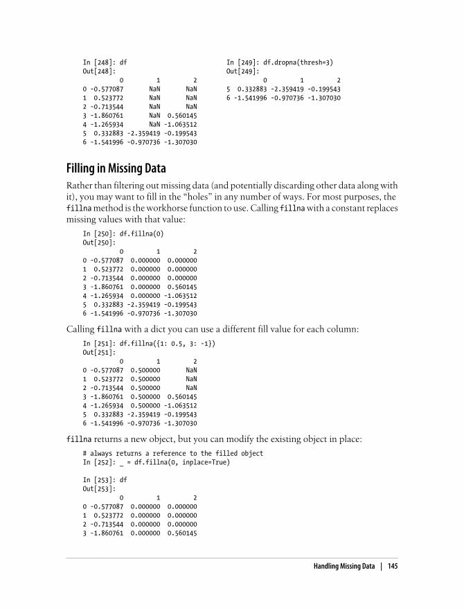
In [248]: df In [249]: df.dropna(thresh=3) Out[248]: Out[249]: 0 1 2 0 1 20 -0.577087 NaN NaN 5 0.332883 -2.359419 -0.1995431 0.523772 NaN NaN 6 -1.541996 -0.970736 -1.3070302 -0.713544 NaN NaN 3 -1.860761 NaN 0.560145 4 -1.265934 NaN -1.063512 5 0.332883 -2.359419 -0.199543 6 -1.541996 -0.970736 -1.307030
Filling in Missing DataRather than filtering out missing data (and potentially discarding other data along withit), you may want to fill in the “holes” in any number of ways. For most purposes, the fillna method is the workhorse function to use. Calling fillna with a constant replacesmissing values with that value:
In [250]: df.fillna(0)Out[250]: 0 1 20 -0.577087 0.000000 0.0000001 0.523772 0.000000 0.0000002 -0.713544 0.000000 0.0000003 -1.860761 0.000000 0.5601454 -1.265934 0.000000 -1.0635125 0.332883 -2.359419 -0.1995436 -1.541996 -0.970736 -1.307030
Calling fillna with a dict you can use a different fill value for each column:
In [251]: df.fillna({1: 0.5, 3: -1})Out[251]: 0 1 20 -0.577087 0.500000 NaN1 0.523772 0.500000 NaN2 -0.713544 0.500000 NaN3 -1.860761 0.500000 0.5601454 -1.265934 0.500000 -1.0635125 0.332883 -2.359419 -0.1995436 -1.541996 -0.970736 -1.307030
fillna returns a new object, but you can modify the existing object in place:
# always returns a reference to the filled objectIn [252]: _ = df.fillna(0, inplace=True)
In [253]: dfOut[253]: 0 1 20 -0.577087 0.000000 0.0000001 0.523772 0.000000 0.0000002 -0.713544 0.000000 0.0000003 -1.860761 0.000000 0.560145
Handling Missing Data | 145

4 -1.265934 0.000000 -1.0635125 0.332883 -2.359419 -0.1995436 -1.541996 -0.970736 -1.307030
The same interpolation methods available for reindexing can be used with fillna:
In [254]: df = DataFrame(np.random.randn(6, 3))
In [255]: df.ix[2:, 1] = NA; df.ix[4:, 2] = NA
In [256]: dfOut[256]: 0 1 20 0.286350 0.377984 -0.7538871 0.331286 1.349742 0.0698772 0.246674 NaN 1.0048123 1.327195 NaN -1.5491064 0.022185 NaN NaN5 0.862580 NaN NaN
In [257]: df.fillna(method='ffill') In [258]: df.fillna(method='ffill', limit=2)Out[257]: Out[258]: 0 1 2 0 1 2 0 0.286350 0.377984 -0.753887 0 0.286350 0.377984 -0.753887 1 0.331286 1.349742 0.069877 1 0.331286 1.349742 0.069877 2 0.246674 1.349742 1.004812 2 0.246674 1.349742 1.004812 3 1.327195 1.349742 -1.549106 3 1.327195 1.349742 -1.549106 4 0.022185 1.349742 -1.549106 4 0.022185 NaN -1.549106 5 0.862580 1.349742 -1.549106 5 0.862580 NaN -1.549106
With fillna you can do lots of other things with a little creativity. For example, youmight pass the mean or median value of a Series:
In [259]: data = Series([1., NA, 3.5, NA, 7])
In [260]: data.fillna(data.mean())Out[260]: 0 1.0000001 3.8333332 3.5000003 3.8333334 7.000000
See Table 5-13 for a reference on fillna.
Table 5-13. fillna function arguments
Argument Description
value Scalar value or dict-like object to use to fill missing values
method Interpolation, by default 'ffill' if function called with no other arguments
axis Axis to fill on, default axis=0
inplace Modify the calling object without producing a copy
limit For forward and backward filling, maximum number of consecutive periods to fill
146 | Chapter 5: Getting Started with pandas

Hierarchical IndexingHierarchical indexing is an important feature of pandas enabling you to have multiple(two or more) index levels on an axis. Somewhat abstractly, it provides a way for youto work with higher dimensional data in a lower dimensional form. Let’s start with asimple example; create a Series with a list of lists or arrays as the index:
In [261]: data = Series(np.random.randn(10), .....: index=[['a', 'a', 'a', 'b', 'b', 'b', 'c', 'c', 'd', 'd'], .....: [1, 2, 3, 1, 2, 3, 1, 2, 2, 3]])
In [262]: dataOut[262]: a 1 0.670216 2 0.852965 3 -0.955869b 1 -0.023493 2 -2.304234 3 -0.652469c 1 -1.218302 2 -1.332610d 2 1.074623 3 0.723642
What you’re seeing is a prettified view of a Series with a MultiIndex as its index. The“gaps” in the index display mean “use the label directly above”:
In [263]: data.indexOut[263]: MultiIndex[('a', 1) ('a', 2) ('a', 3) ('b', 1) ('b', 2) ('b', 3) ('c', 1) ('c', 2) ('d', 2) ('d', 3)]
With a hierarchically-indexed object, so-called partial indexing is possible, enablingyou to concisely select subsets of the data:
In [264]: data['b']Out[264]: 1 -0.0234932 -2.3042343 -0.652469
In [265]: data['b':'c'] In [266]: data.ix[['b', 'd']]Out[265]: Out[266]: b 1 -0.023493 b 1 -0.023493 2 -2.304234 2 -2.304234 3 -0.652469 3 -0.652469 c 1 -1.218302 d 2 1.074623 2 -1.332610 3 0.723642
Selection is even possible in some cases from an “inner” level:
In [267]: data[:, 2]Out[267]: a 0.852965
Hierarchical Indexing | 147

b -2.304234c -1.332610d 1.074623
Hierarchical indexing plays a critical role in reshaping data and group-based operationslike forming a pivot table. For example, this data could be rearranged into a DataFrameusing its unstack method:
In [268]: data.unstack()Out[268]: 1 2 3a 0.670216 0.852965 -0.955869b -0.023493 -2.304234 -0.652469c -1.218302 -1.332610 NaNd NaN 1.074623 0.723642
The inverse operation of unstack is stack:
In [269]: data.unstack().stack()Out[269]: a 1 0.670216 2 0.852965 3 -0.955869b 1 -0.023493 2 -2.304234 3 -0.652469c 1 -1.218302 2 -1.332610d 2 1.074623 3 0.723642
stack and unstack will be explored in more detail in Chapter 7.
With a DataFrame, either axis can have a hierarchical index:
In [270]: frame = DataFrame(np.arange(12).reshape((4, 3)), .....: index=[['a', 'a', 'b', 'b'], [1, 2, 1, 2]], .....: columns=[['Ohio', 'Ohio', 'Colorado'], .....: ['Green', 'Red', 'Green']])
In [271]: frameOut[271]: Ohio Colorado Green Red Greena 1 0 1 2 2 3 4 5b 1 6 7 8 2 9 10 11
The hierarchical levels can have names (as strings or any Python objects). If so, thesewill show up in the console output (don’t confuse the index names with the axis labels!):
In [272]: frame.index.names = ['key1', 'key2']
In [273]: frame.columns.names = ['state', 'color']
In [274]: frame
148 | Chapter 5: Getting Started with pandas
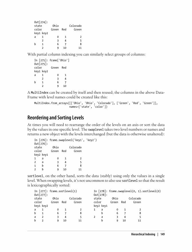
Out[274]: state Ohio Coloradocolor Green Red Greenkey1 key2 a 1 0 1 2 2 3 4 5b 1 6 7 8 2 9 10 11
With partial column indexing you can similarly select groups of columns:
In [275]: frame['Ohio']Out[275]: color Green Redkey1 key2 a 1 0 1 2 3 4b 1 6 7 2 9 10
A MultiIndex can be created by itself and then reused; the columns in the above Data-Frame with level names could be created like this:
MultiIndex.from_arrays([['Ohio', 'Ohio', 'Colorado'], ['Green', 'Red', 'Green']], names=['state', 'color'])
Reordering and Sorting LevelsAt times you will need to rearrange the order of the levels on an axis or sort the databy the values in one specific level. The swaplevel takes two level numbers or names andreturns a new object with the levels interchanged (but the data is otherwise unaltered):
In [276]: frame.swaplevel('key1', 'key2')Out[276]: state Ohio Coloradocolor Green Red Greenkey2 key1 1 a 0 1 22 a 3 4 51 b 6 7 82 b 9 10 11
sortlevel, on the other hand, sorts the data (stably) using only the values in a singlelevel. When swapping levels, it’s not uncommon to also use sortlevel so that the resultis lexicographically sorted:
In [277]: frame.sortlevel(1) In [278]: frame.swaplevel(0, 1).sortlevel(0)Out[277]: Out[278]: state Ohio Colorado state Ohio Colorado color Green Red Green color Green Red Green key1 key2 key2 key1 a 1 0 1 2 1 a 0 1 2 b 1 6 7 8 b 6 7 8 a 2 3 4 5 2 a 3 4 5 b 2 9 10 11 b 9 10 11
Hierarchical Indexing | 149

Data selection performance is much better on hierarchically indexedobjects if the index is lexicographically sorted starting with the outer-most level, that is, the result of calling sortlevel(0) or sort_index().
Summary Statistics by LevelMany descriptive and summary statistics on DataFrame and Series have a level optionin which you can specify the level you want to sum by on a particular axis. Considerthe above DataFrame; we can sum by level on either the rows or columns like so:
In [279]: frame.sum(level='key2')Out[279]: state Ohio Coloradocolor Green Red Greenkey2 1 6 8 102 12 14 16
In [280]: frame.sum(level='color', axis=1)Out[280]: color Green Redkey1 key2 a 1 2 1 2 8 4b 1 14 7 2 20 10
Under the hood, this utilizes pandas’s groupby machinery which will be discussed inmore detail later in the book.
Using a DataFrame’s ColumnsIt’s not unusual to want to use one or more columns from a DataFrame as the rowindex; alternatively, you may wish to move the row index into the DataFrame’s col-umns. Here’s an example DataFrame:
In [281]: frame = DataFrame({'a': range(7), 'b': range(7, 0, -1), .....: 'c': ['one', 'one', 'one', 'two', 'two', 'two', 'two'], .....: 'd': [0, 1, 2, 0, 1, 2, 3]})
In [282]: frameOut[282]: a b c d0 0 7 one 01 1 6 one 12 2 5 one 23 3 4 two 04 4 3 two 15 5 2 two 26 6 1 two 3
150 | Chapter 5: Getting Started with pandas
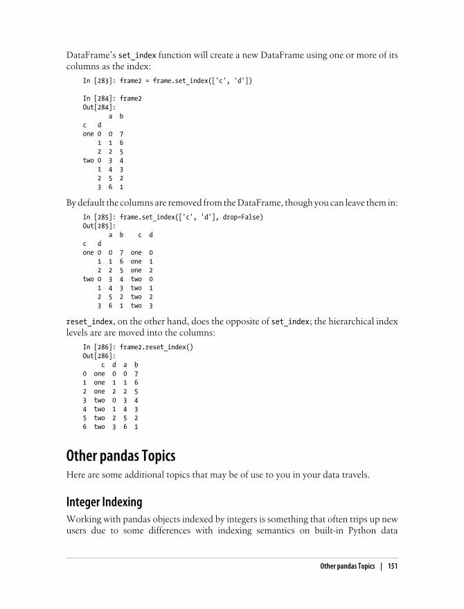
DataFrame’s set_index function will create a new DataFrame using one or more of itscolumns as the index:
In [283]: frame2 = frame.set_index(['c', 'd'])
In [284]: frame2Out[284]: a bc d one 0 0 7 1 1 6 2 2 5two 0 3 4 1 4 3 2 5 2 3 6 1
By default the columns are removed from the DataFrame, though you can leave them in:
In [285]: frame.set_index(['c', 'd'], drop=False)Out[285]: a b c dc d one 0 0 7 one 0 1 1 6 one 1 2 2 5 one 2two 0 3 4 two 0 1 4 3 two 1 2 5 2 two 2 3 6 1 two 3
reset_index, on the other hand, does the opposite of set_index; the hierarchical indexlevels are are moved into the columns:
In [286]: frame2.reset_index()Out[286]: c d a b0 one 0 0 71 one 1 1 62 one 2 2 53 two 0 3 44 two 1 4 35 two 2 5 26 two 3 6 1
Other pandas TopicsHere are some additional topics that may be of use to you in your data travels.
Integer IndexingWorking with pandas objects indexed by integers is something that often trips up newusers due to some differences with indexing semantics on built-in Python data
Other pandas Topics | 151

structures like lists and tuples. For example, you would not expect the following codeto generate an error:
ser = Series(np.arange(3.))ser[-1]
In this case, pandas could “fall back” on integer indexing, but there’s not a safe andgeneral way (that I know of) to do this without introducing subtle bugs. Here we havean index containing 0, 1, 2, but inferring what the user wants (label-based indexing orposition-based) is difficult::
In [288]: serOut[288]: 0 01 12 2
On the other hand, with a non-integer index, there is no potential for ambiguity:
In [289]: ser2 = Series(np.arange(3.), index=['a', 'b', 'c'])
In [290]: ser2[-1]Out[290]: 2.0
To keep things consistent, if you have an axis index containing indexers, data selectionwith integers will always be label-oriented. This includes slicing with ix, too:
In [291]: ser.ix[:1]Out[291]: 0 01 1
In cases where you need reliable position-based indexing regardless of the index type,you can use the iget_value method from Series and irow and icol methods from Da-taFrame:
In [292]: ser3 = Series(range(3), index=[-5, 1, 3])
In [293]: ser3.iget_value(2)Out[293]: 2
In [294]: frame = DataFrame(np.arange(6).reshape(3, 2)), index=[2, 0, 1])
In [295]: frame.irow(0)Out[295]: 0 01 1Name: 2
Panel DataWhile not a major topic of this book, pandas has a Panel data structure, which you canthink of as a three-dimensional analogue of DataFrame. Much of the development focusof pandas has been in tabular data manipulations as these are easier to reason about,
152 | Chapter 5: Getting Started with pandas
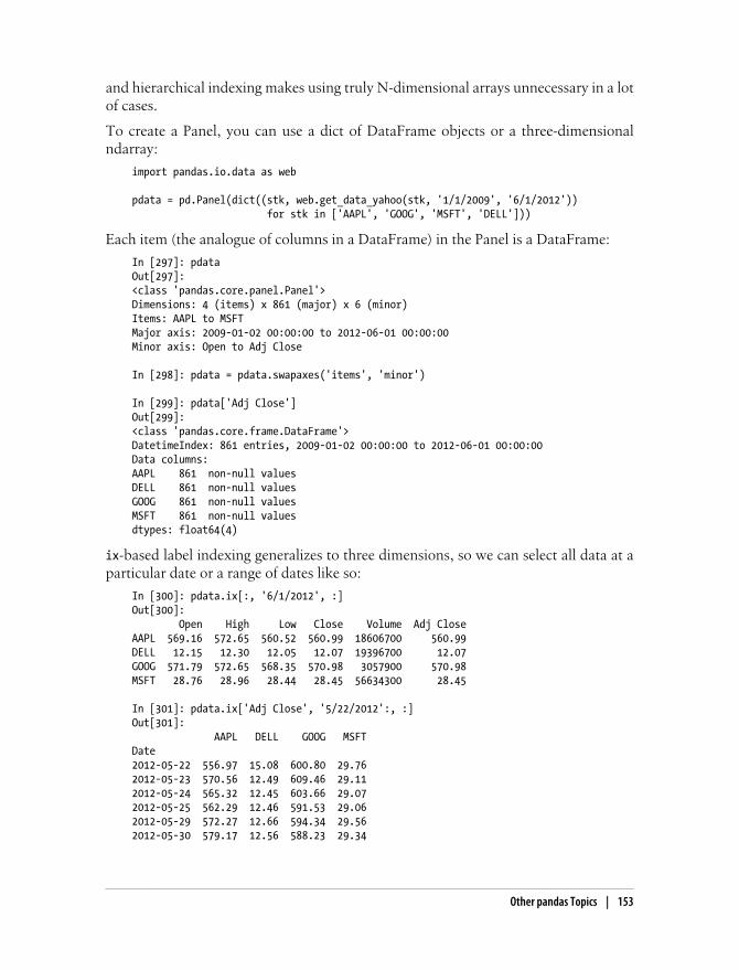
and hierarchical indexing makes using truly N-dimensional arrays unnecessary in a lotof cases.
To create a Panel, you can use a dict of DataFrame objects or a three-dimensionalndarray:
import pandas.io.data as web
pdata = pd.Panel(dict((stk, web.get_data_yahoo(stk, '1/1/2009', '6/1/2012')) for stk in ['AAPL', 'GOOG', 'MSFT', 'DELL']))
Each item (the analogue of columns in a DataFrame) in the Panel is a DataFrame:
In [297]: pdataOut[297]: <class 'pandas.core.panel.Panel'>Dimensions: 4 (items) x 861 (major) x 6 (minor)Items: AAPL to MSFTMajor axis: 2009-01-02 00:00:00 to 2012-06-01 00:00:00Minor axis: Open to Adj Close
In [298]: pdata = pdata.swapaxes('items', 'minor')
In [299]: pdata['Adj Close']Out[299]: <class 'pandas.core.frame.DataFrame'>DatetimeIndex: 861 entries, 2009-01-02 00:00:00 to 2012-06-01 00:00:00Data columns:AAPL 861 non-null valuesDELL 861 non-null valuesGOOG 861 non-null valuesMSFT 861 non-null valuesdtypes: float64(4)
ix-based label indexing generalizes to three dimensions, so we can select all data at aparticular date or a range of dates like so:
In [300]: pdata.ix[:, '6/1/2012', :]Out[300]: Open High Low Close Volume Adj CloseAAPL 569.16 572.65 560.52 560.99 18606700 560.99DELL 12.15 12.30 12.05 12.07 19396700 12.07GOOG 571.79 572.65 568.35 570.98 3057900 570.98MSFT 28.76 28.96 28.44 28.45 56634300 28.45
In [301]: pdata.ix['Adj Close', '5/22/2012':, :]Out[301]: AAPL DELL GOOG MSFTDate 2012-05-22 556.97 15.08 600.80 29.762012-05-23 570.56 12.49 609.46 29.112012-05-24 565.32 12.45 603.66 29.072012-05-25 562.29 12.46 591.53 29.062012-05-29 572.27 12.66 594.34 29.562012-05-30 579.17 12.56 588.23 29.34
Other pandas Topics | 153

2012-05-31 577.73 12.33 580.86 29.192012-06-01 560.99 12.07 570.98 28.45
An alternate way to represent panel data, especially for fitting statistical models, is in“stacked” DataFrame form:
In [302]: stacked = pdata.ix[:, '5/30/2012':, :].to_frame()
In [303]: stackedOut[303]: Open High Low Close Volume Adj Closemajor minor 2012-05-30 AAPL 569.20 579.99 566.56 579.17 18908200 579.17 DELL 12.59 12.70 12.46 12.56 19787800 12.56 GOOG 588.16 591.90 583.53 588.23 1906700 588.23 MSFT 29.35 29.48 29.12 29.34 41585500 29.342012-05-31 AAPL 580.74 581.50 571.46 577.73 17559800 577.73 DELL 12.53 12.54 12.33 12.33 19955500 12.33 GOOG 588.72 590.00 579.00 580.86 2968300 580.86 MSFT 29.30 29.42 28.94 29.19 39134000 29.192012-06-01 AAPL 569.16 572.65 560.52 560.99 18606700 560.99 DELL 12.15 12.30 12.05 12.07 19396700 12.07 GOOG 571.79 572.65 568.35 570.98 3057900 570.98 MSFT 28.76 28.96 28.44 28.45 56634300 28.45
DataFrame has a related to_panel method, the inverse of to_frame:
In [304]: stacked.to_panel()Out[304]: <class 'pandas.core.panel.Panel'>Dimensions: 6 (items) x 3 (major) x 4 (minor)Items: Open to Adj CloseMajor axis: 2012-05-30 00:00:00 to 2012-06-01 00:00:00Minor axis: AAPL to MSFT
154 | Chapter 5: Getting Started with pandas

CHAPTER 6
Data Loading, Storage, and FileFormats
The tools in this book are of little use if you can’t easily import and export data inPython. I’m going to be focused on input and output with pandas objects, though thereare of course numerous tools in other libraries to aid in this process. NumPy, for ex-ample, features low-level but extremely fast binary data loading and storage, includingsupport for memory-mapped array. See Chapter 12 for more on those.
Input and output typically falls into a few main categories: reading text files and othermore efficient on-disk formats, loading data from databases, and interacting with net-work sources like web APIs.
Reading and Writing Data in Text FormatPython has become a beloved language for text and file munging due to its simple syntaxfor interacting with files, intuitive data structures, and convenient features like tuplepacking and unpacking.
pandas features a number of functions for reading tabular data as a DataFrame object.Table 6-1 has a summary of all of them, though read_csv and read_table are likely theones you’ll use the most.
Table 6-1. Parsing functions in pandas
Function Description
read_csv Load delimited data from a file, URL, or file-like object. Use comma as default delimiter
read_table Load delimited data from a file, URL, or file-like object. Use tab ('\t') as default delimiter
read_fwf Read data in fixed-width column format (that is, no delimiters)
read_clipboard Version of read_table that reads data from the clipboard. Useful for converting tables from web pages
155
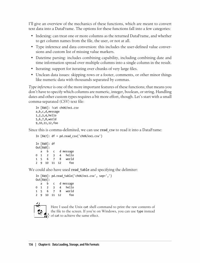
I’ll give an overview of the mechanics of these functions, which are meant to converttext data into a DataFrame. The options for these functions fall into a few categories:
• Indexing: can treat one or more columns as the returned DataFrame, and whetherto get column names from the file, the user, or not at all.
• Type inference and data conversion: this includes the user-defined value conver-sions and custom list of missing value markers.
• Datetime parsing: includes combining capability, including combining date andtime information spread over multiple columns into a single column in the result.
• Iterating: support for iterating over chunks of very large files.
• Unclean data issues: skipping rows or a footer, comments, or other minor thingslike numeric data with thousands separated by commas.
Type inference is one of the more important features of these functions; that means youdon’t have to specify which columns are numeric, integer, boolean, or string. Handlingdates and other custom types requires a bit more effort, though. Let’s start with a smallcomma-separated (CSV) text file:
In [846]: !cat ch06/ex1.csva,b,c,d,message1,2,3,4,hello5,6,7,8,world9,10,11,12,foo
Since this is comma-delimited, we can use read_csv to read it into a DataFrame:
In [847]: df = pd.read_csv('ch06/ex1.csv')
In [848]: dfOut[848]: a b c d message0 1 2 3 4 hello1 5 6 7 8 world2 9 10 11 12 foo
We could also have used read_table and specifying the delimiter:
In [849]: pd.read_table('ch06/ex1.csv', sep=',')Out[849]: a b c d message0 1 2 3 4 hello1 5 6 7 8 world2 9 10 11 12 foo
Here I used the Unix cat shell command to print the raw contents ofthe file to the screen. If you’re on Windows, you can use type insteadof cat to achieve the same effect.
156 | Chapter 6: Data Loading, Storage, and File Formats
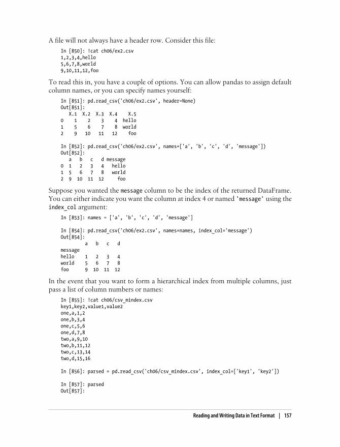
A file will not always have a header row. Consider this file:
In [850]: !cat ch06/ex2.csv1,2,3,4,hello5,6,7,8,world9,10,11,12,foo
To read this in, you have a couple of options. You can allow pandas to assign defaultcolumn names, or you can specify names yourself:
In [851]: pd.read_csv('ch06/ex2.csv', header=None)Out[851]: X.1 X.2 X.3 X.4 X.50 1 2 3 4 hello1 5 6 7 8 world2 9 10 11 12 foo
In [852]: pd.read_csv('ch06/ex2.csv', names=['a', 'b', 'c', 'd', 'message'])Out[852]: a b c d message0 1 2 3 4 hello1 5 6 7 8 world2 9 10 11 12 foo
Suppose you wanted the message column to be the index of the returned DataFrame.You can either indicate you want the column at index 4 or named 'message' using theindex_col argument:
In [853]: names = ['a', 'b', 'c', 'd', 'message']
In [854]: pd.read_csv('ch06/ex2.csv', names=names, index_col='message')Out[854]: a b c dmessage hello 1 2 3 4world 5 6 7 8foo 9 10 11 12
In the event that you want to form a hierarchical index from multiple columns, justpass a list of column numbers or names:
In [855]: !cat ch06/csv_mindex.csvkey1,key2,value1,value2one,a,1,2one,b,3,4one,c,5,6one,d,7,8two,a,9,10two,b,11,12two,c,13,14two,d,15,16
In [856]: parsed = pd.read_csv('ch06/csv_mindex.csv', index_col=['key1', 'key2'])
In [857]: parsedOut[857]:
Reading and Writing Data in Text Format | 157

value1 value2key1 key2 one a 1 2 b 3 4 c 5 6 d 7 8two a 9 10 b 11 12 c 13 14 d 15 16
In some cases, a table might not have a fixed delimiter, using whitespace or some otherpattern to separate fields. In these cases, you can pass a regular expression as a delimiterfor read_table. Consider a text file that looks like this:
In [858]: list(open('ch06/ex3.txt'))Out[858]: [' A B C\n', 'aaa -0.264438 -1.026059 -0.619500\n', 'bbb 0.927272 0.302904 -0.032399\n', 'ccc -0.264273 -0.386314 -0.217601\n', 'ddd -0.871858 -0.348382 1.100491\n']
While you could do some munging by hand, in this case fields are separated by a variableamount of whitespace. This can be expressed by the regular expression \s+, so we havethen:
In [859]: result = pd.read_table('ch06/ex3.txt', sep='\s+')
In [860]: resultOut[860]: A B Caaa -0.264438 -1.026059 -0.619500bbb 0.927272 0.302904 -0.032399ccc -0.264273 -0.386314 -0.217601ddd -0.871858 -0.348382 1.100491
Because there was one fewer column name than the number of data rows, read_tableinfers that the first column should be the DataFrame’s index in this special case.
The parser functions have many additional arguments to help you handle the widevariety of exception file formats that occur (see Table 6-2). For example, you can skipthe first, third, and fourth rows of a file with skiprows:
In [861]: !cat ch06/ex4.csv# hey!a,b,c,d,message# just wanted to make things more difficult for you# who reads CSV files with computers, anyway?1,2,3,4,hello5,6,7,8,world9,10,11,12,fooIn [862]: pd.read_csv('ch06/ex4.csv', skiprows=[0, 2, 3])Out[862]: a b c d message
158 | Chapter 6: Data Loading, Storage, and File Formats

0 1 2 3 4 hello1 5 6 7 8 world2 9 10 11 12 foo
Handling missing values is an important and frequently nuanced part of the file parsingprocess. Missing data is usually either not present (empty string) or marked by some sentinel value. By default, pandas uses a set of commonly occurring sentinels, such asNA, -1.#IND, and NULL:
In [863]: !cat ch06/ex5.csvsomething,a,b,c,d,messageone,1,2,3,4,NAtwo,5,6,,8,worldthree,9,10,11,12,fooIn [864]: result = pd.read_csv('ch06/ex5.csv')
In [865]: resultOut[865]: something a b c d message0 one 1 2 3 4 NaN1 two 5 6 NaN 8 world2 three 9 10 11 12 foo
In [866]: pd.isnull(result)Out[866]: something a b c d message0 False False False False False True1 False False False True False False2 False False False False False False
The na_values option can take either a list or set of strings to consider missing values:
In [867]: result = pd.read_csv('ch06/ex5.csv', na_values=['NULL'])
In [868]: resultOut[868]: something a b c d message0 one 1 2 3 4 NaN1 two 5 6 NaN 8 world2 three 9 10 11 12 foo
Different NA sentinels can be specified for each column in a dict:
In [869]: sentinels = {'message': ['foo', 'NA'], 'something': ['two']}
In [870]: pd.read_csv('ch06/ex5.csv', na_values=sentinels)Out[870]: something a b c d message0 one 1 2 3 4 NaN1 NaN 5 6 NaN 8 world2 three 9 10 11 12 NaN
Reading and Writing Data in Text Format | 159
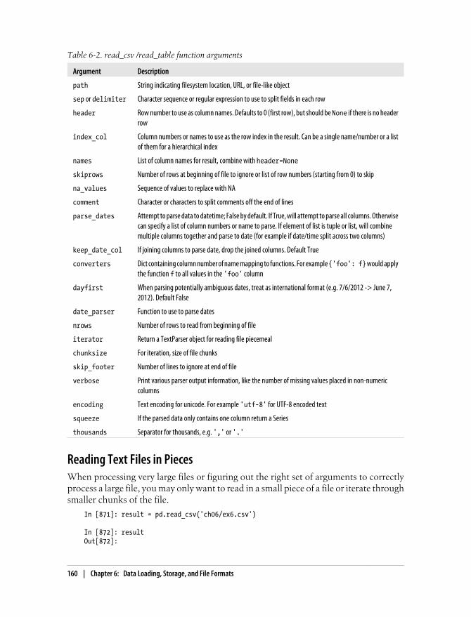
Table 6-2. read_csv /read_table function arguments
Argument Description
path String indicating filesystem location, URL, or file-like object
sep or delimiter Character sequence or regular expression to use to split fields in each row
header Row number to use as column names. Defaults to 0 (first row), but should be None if there is no headerrow
index_col Column numbers or names to use as the row index in the result. Can be a single name/number or a listof them for a hierarchical index
names List of column names for result, combine with header=None
skiprows Number of rows at beginning of file to ignore or list of row numbers (starting from 0) to skip
na_values Sequence of values to replace with NA
comment Character or characters to split comments off the end of lines
parse_dates Attempt to parse data to datetime; False by default. If True, will attempt to parse all columns. Otherwisecan specify a list of column numbers or name to parse. If element of list is tuple or list, will combinemultiple columns together and parse to date (for example if date/time split across two columns)
keep_date_col If joining columns to parse date, drop the joined columns. Default True
converters Dict containing column number of name mapping to functions. For example {'foo': f} would applythe function f to all values in the 'foo' column
dayfirst When parsing potentially ambiguous dates, treat as international format (e.g. 7/6/2012 -> June 7,2012). Default False
date_parser Function to use to parse dates
nrows Number of rows to read from beginning of file
iterator Return a TextParser object for reading file piecemeal
chunksize For iteration, size of file chunks
skip_footer Number of lines to ignore at end of file
verbose Print various parser output information, like the number of missing values placed in non-numericcolumns
encoding Text encoding for unicode. For example 'utf-8' for UTF-8 encoded text
squeeze If the parsed data only contains one column return a Series
thousands Separator for thousands, e.g. ',' or '.'
Reading Text Files in PiecesWhen processing very large files or figuring out the right set of arguments to correctlyprocess a large file, you may only want to read in a small piece of a file or iterate throughsmaller chunks of the file.
In [871]: result = pd.read_csv('ch06/ex6.csv')
In [872]: resultOut[872]:
160 | Chapter 6: Data Loading, Storage, and File Formats

<class 'pandas.core.frame.DataFrame'>Int64Index: 10000 entries, 0 to 9999Data columns:one 10000 non-null valuestwo 10000 non-null valuesthree 10000 non-null valuesfour 10000 non-null valueskey 10000 non-null valuesdtypes: float64(4), object(1)
If you want to only read out a small number of rows (avoiding reading the entire file),specify that with nrows:
In [873]: pd.read_csv('ch06/ex6.csv', nrows=5)Out[873]: one two three four key0 0.467976 -0.038649 -0.295344 -1.824726 L1 -0.358893 1.404453 0.704965 -0.200638 B2 -0.501840 0.659254 -0.421691 -0.057688 G3 0.204886 1.074134 1.388361 -0.982404 R4 0.354628 -0.133116 0.283763 -0.837063 Q
To read out a file in pieces, specify a chunksize as a number of rows:
In [874]: chunker = pd.read_csv('ch06/ex6.csv', chunksize=1000)
In [875]: chunkerOut[875]: <pandas.io.parsers.TextParser at 0x8398150>
The TextParser object returned by read_csv allows you to iterate over the parts of thefile according to the chunksize. For example, we can iterate over ex6.csv, aggregatingthe value counts in the 'key' column like so:
chunker = pd.read_csv('ch06/ex6.csv', chunksize=1000)
tot = Series([])for piece in chunker: tot = tot.add(piece['key'].value_counts(), fill_value=0)
tot = tot.order(ascending=False)
We have then:
In [877]: tot[:10]Out[877]: E 368X 364L 346O 343Q 340M 338J 337F 335K 334H 330
Reading and Writing Data in Text Format | 161
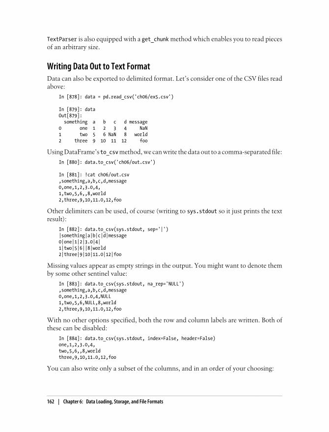
TextParser is also equipped with a get_chunk method which enables you to read piecesof an arbitrary size.
Writing Data Out to Text FormatData can also be exported to delimited format. Let’s consider one of the CSV files readabove:
In [878]: data = pd.read_csv('ch06/ex5.csv')
In [879]: dataOut[879]: something a b c d message0 one 1 2 3 4 NaN1 two 5 6 NaN 8 world2 three 9 10 11 12 foo
Using DataFrame’s to_csv method, we can write the data out to a comma-separated file:
In [880]: data.to_csv('ch06/out.csv')
In [881]: !cat ch06/out.csv,something,a,b,c,d,message0,one,1,2,3.0,4,1,two,5,6,,8,world2,three,9,10,11.0,12,foo
Other delimiters can be used, of course (writing to sys.stdout so it just prints the textresult):
In [882]: data.to_csv(sys.stdout, sep='|')|something|a|b|c|d|message0|one|1|2|3.0|4|1|two|5|6||8|world2|three|9|10|11.0|12|foo
Missing values appear as empty strings in the output. You might want to denote themby some other sentinel value:
In [883]: data.to_csv(sys.stdout, na_rep='NULL'),something,a,b,c,d,message0,one,1,2,3.0,4,NULL1,two,5,6,NULL,8,world2,three,9,10,11.0,12,foo
With no other options specified, both the row and column labels are written. Both ofthese can be disabled:
In [884]: data.to_csv(sys.stdout, index=False, header=False)one,1,2,3.0,4,two,5,6,,8,worldthree,9,10,11.0,12,foo
You can also write only a subset of the columns, and in an order of your choosing:
162 | Chapter 6: Data Loading, Storage, and File Formats

In [885]: data.to_csv(sys.stdout, index=False, cols=['a', 'b', 'c'])a,b,c1,2,3.05,6,9,10,11.0
Series also has a to_csv method:
In [886]: dates = pd.date_range('1/1/2000', periods=7)
In [887]: ts = Series(np.arange(7), index=dates)
In [888]: ts.to_csv('ch06/tseries.csv')
In [889]: !cat ch06/tseries.csv2000-01-01 00:00:00,02000-01-02 00:00:00,12000-01-03 00:00:00,22000-01-04 00:00:00,32000-01-05 00:00:00,42000-01-06 00:00:00,52000-01-07 00:00:00,6
With a bit of wrangling (no header, first column as index), you can read a CSV versionof a Series with read_csv, but there is also a from_csv convenience method that makesit a bit simpler:
In [890]: Series.from_csv('ch06/tseries.csv', parse_dates=True)Out[890]: 2000-01-01 02000-01-02 12000-01-03 22000-01-04 32000-01-05 42000-01-06 52000-01-07 6
See the docstrings for to_csv and from_csv in IPython for more information.
Manually Working with Delimited FormatsMost forms of tabular data can be loaded from disk using functions like pandas.read_table. In some cases, however, some manual processing may be necessary.It’s not uncommon to receive a file with one or more malformed lines that trip up read_table. To illustrate the basic tools, consider a small CSV file:
In [891]: !cat ch06/ex7.csv"a","b","c""1","2","3""1","2","3","4"
For any file with a single-character delimiter, you can use Python’s built-in csv module.To use it, pass any open file or file-like object to csv.reader:
Reading and Writing Data in Text Format | 163
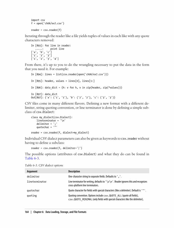
import csvf = open('ch06/ex7.csv')
reader = csv.reader(f)
Iterating through the reader like a file yields tuples of values in each like with any quotecharacters removed:
In [893]: for line in reader: .....: print line['a', 'b', 'c']['1', '2', '3']['1', '2', '3', '4']
From there, it’s up to you to do the wrangling necessary to put the data in the formthat you need it. For example:
In [894]: lines = list(csv.reader(open('ch06/ex7.csv')))
In [895]: header, values = lines[0], lines[1:]
In [896]: data_dict = {h: v for h, v in zip(header, zip(*values))}
In [897]: data_dictOut[897]: {'a': ('1', '1'), 'b': ('2', '2'), 'c': ('3', '3')}
CSV files come in many different flavors. Defining a new format with a different de-limiter, string quoting convention, or line terminator is done by defining a simple sub-class of csv.Dialect:
class my_dialect(csv.Dialect): lineterminator = '\n' delimiter = ';' quotechar = '"'
reader = csv.reader(f, dialect=my_dialect)
Individual CSV dialect parameters can also be given as keywords to csv.reader withouthaving to define a subclass:
reader = csv.reader(f, delimiter='|')
The possible options (attributes of csv.Dialect) and what they do can be found inTable 6-3.
Table 6-3. CSV dialect options
Argument Description
delimiter One-character string to separate fields. Defaults to ','.
lineterminator Line terminator for writing, defaults to '\r\n'. Reader ignores this and recognizescross-platform line terminators.
quotechar Quote character for fields with special characters (like a delimiter). Default is '"'.
quoting Quoting convention. Options include csv.QUOTE_ALL (quote all fields),csv.QUOTE_MINIMAL (only fields with special characters like the delimiter),
164 | Chapter 6: Data Loading, Storage, and File Formats

Argument Descriptioncsv.QUOTE_NONNUMERIC, and csv.QUOTE_NON (no quoting). See Python’sdocumentation for full details. Defaults to QUOTE_MINIMAL.
skipinitialspace Ignore whitespace after each delimiter. Default False.
doublequote How to handle quoting character inside a field. If True, it is doubled. See onlinedocumentation for full detail and behavior.
escapechar String to escape the delimiter if quoting is set to csv.QUOTE_NONE. Disabled bydefault
For files with more complicated or fixed multicharacter delimiters, youwill not be able to use the csv module. In those cases, you’ll have to dothe line splitting and other cleanup using string’s split method or theregular expression method re.split.
To write delimited files manually, you can use csv.writer. It accepts an open, writablefile object and the same dialect and format options as csv.reader:
with open('mydata.csv', 'w') as f: writer = csv.writer(f, dialect=my_dialect) writer.writerow(('one', 'two', 'three')) writer.writerow(('1', '2', '3')) writer.writerow(('4', '5', '6')) writer.writerow(('7', '8', '9'))
JSON DataJSON (short for JavaScript Object Notation) has become one of the standard formatsfor sending data by HTTP request between web browsers and other applications. It isa much more flexible data format than a tabular text form like CSV. Here is an example:
obj = """{"name": "Wes", "places_lived": ["United States", "Spain", "Germany"], "pet": null, "siblings": [{"name": "Scott", "age": 25, "pet": "Zuko"}, {"name": "Katie", "age": 33, "pet": "Cisco"}]}"""
JSON is very nearly valid Python code with the exception of its null value null andsome other nuances (such as disallowing trailing commas at the end of lists). The basictypes are objects (dicts), arrays (lists), strings, numbers, booleans, and nulls. All of thekeys in an object must be strings. There are several Python libraries for reading andwriting JSON data. I’ll use json here as it is built into the Python standard library. Toconvert a JSON string to Python form, use json.loads:
In [899]: import json
Reading and Writing Data in Text Format | 165
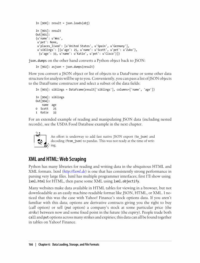
In [900]: result = json.loads(obj)
In [901]: resultOut[901]: {u'name': u'Wes', u'pet': None, u'places_lived': [u'United States', u'Spain', u'Germany'], u'siblings': [{u'age': 25, u'name': u'Scott', u'pet': u'Zuko'}, {u'age': 33, u'name': u'Katie', u'pet': u'Cisco'}]}
json.dumps on the other hand converts a Python object back to JSON:
In [902]: asjson = json.dumps(result)
How you convert a JSON object or list of objects to a DataFrame or some other datastructure for analysis will be up to you. Conveniently, you can pass a list of JSON objectsto the DataFrame constructor and select a subset of the data fields:
In [903]: siblings = DataFrame(result['siblings'], columns=['name', 'age'])
In [904]: siblingsOut[904]: name age0 Scott 251 Katie 33
For an extended example of reading and manipulating JSON data (including nestedrecords), see the USDA Food Database example in the next chapter.
An effort is underway to add fast native JSON export (to_json) anddecoding (from_json) to pandas. This was not ready at the time of writ-ing.
XML and HTML: Web ScrapingPython has many libraries for reading and writing data in the ubiquitous HTML andXML formats. lxml (http://lxml.de) is one that has consistently strong performance inparsing very large files. lxml has multiple programmer interfaces; first I’ll show using lxml.html for HTML, then parse some XML using lxml.objectify.
Many websites make data available in HTML tables for viewing in a browser, but notdownloadable as an easily machine-readable format like JSON, HTML, or XML. I no-ticed that this was the case with Yahoo! Finance’s stock options data. If you aren’tfamiliar with this data; options are derivative contracts giving you the right to buy(call option) or sell (put option) a company’s stock at some particular price (thestrike) between now and some fixed point in the future (the expiry). People trade bothcall and put options across many strikes and expiries; this data can all be found togetherin tables on Yahoo! Finance.
166 | Chapter 6: Data Loading, Storage, and File Formats
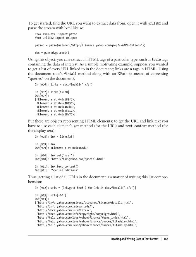
To get started, find the URL you want to extract data from, open it with urllib2 andparse the stream with lxml like so:
from lxml.html import parsefrom urllib2 import urlopen
parsed = parse(urlopen('http://finance.yahoo.com/q/op?s=AAPL+Options'))
doc = parsed.getroot()
Using this object, you can extract all HTML tags of a particular type, such as table tagscontaining the data of interest. As a simple motivating example, suppose you wantedto get a list of every URL linked to in the document; links are a tags in HTML. Usingthe document root’s findall method along with an XPath (a means of expressing“queries” on the document):
In [906]: links = doc.findall('.//a')
In [907]: links[15:20]Out[907]: [<Element a at 0x6c488f0>, <Element a at 0x6c48950>, <Element a at 0x6c489b0>, <Element a at 0x6c48a10>, <Element a at 0x6c48a70>]
But these are objects representing HTML elements; to get the URL and link text youhave to use each element’s get method (for the URL) and text_content method (forthe display text):
In [908]: lnk = links[28]
In [909]: lnkOut[909]: <Element a at 0x6c48dd0>
In [910]: lnk.get('href')Out[910]: 'http://biz.yahoo.com/special.html'
In [911]: lnk.text_content()Out[911]: 'Special Editions'
Thus, getting a list of all URLs in the document is a matter of writing this list compre-hension:
In [912]: urls = [lnk.get('href') for lnk in doc.findall('.//a')]
In [913]: urls[-10:]Out[913]: ['http://info.yahoo.com/privacy/us/yahoo/finance/details.html', 'http://info.yahoo.com/relevantads/', 'http://docs.yahoo.com/info/terms/', 'http://docs.yahoo.com/info/copyright/copyright.html', 'http://help.yahoo.com/l/us/yahoo/finance/forms_index.html', 'http://help.yahoo.com/l/us/yahoo/finance/quotes/fitadelay.html', 'http://help.yahoo.com/l/us/yahoo/finance/quotes/fitadelay.html',
Reading and Writing Data in Text Format | 167
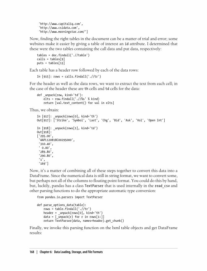
'http://www.capitaliq.com', 'http://www.csidata.com', 'http://www.morningstar.com/']
Now, finding the right tables in the document can be a matter of trial and error; somewebsites make it easier by giving a table of interest an id attribute. I determined thatthese were the two tables containing the call data and put data, respectively:
tables = doc.findall('.//table')calls = tables[9]puts = tables[13]
Each table has a header row followed by each of the data rows:
In [915]: rows = calls.findall('.//tr')
For the header as well as the data rows, we want to extract the text from each cell; inthe case of the header these are th cells and td cells for the data:
def _unpack(row, kind='td'): elts = row.findall('.//%s' % kind) return [val.text_content() for val in elts]
Thus, we obtain:
In [917]: _unpack(rows[0], kind='th')Out[917]: ['Strike', 'Symbol', 'Last', 'Chg', 'Bid', 'Ask', 'Vol', 'Open Int']
In [918]: _unpack(rows[1], kind='td')Out[918]: ['295.00', 'AAPL120818C00295000', '310.40', ' 0.00', '289.80', '290.80', '1', '169']
Now, it’s a matter of combining all of these steps together to convert this data into aDataFrame. Since the numerical data is still in string format, we want to convert some,but perhaps not all of the columns to floating point format. You could do this by hand,but, luckily, pandas has a class TextParser that is used internally in the read_csv andother parsing functions to do the appropriate automatic type conversion:
from pandas.io.parsers import TextParser
def parse_options_data(table): rows = table.findall('.//tr') header = _unpack(rows[0], kind='th') data = [_unpack(r) for r in rows[1:]] return TextParser(data, names=header).get_chunk()
Finally, we invoke this parsing function on the lxml table objects and get DataFrameresults:
168 | Chapter 6: Data Loading, Storage, and File Formats
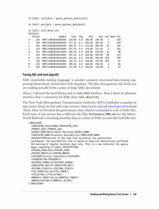
In [920]: call_data = parse_options_data(calls)
In [921]: put_data = parse_options_data(puts)
In [922]: call_data[:10]Out[922]: Strike Symbol Last Chg Bid Ask Vol Open Int0 295 AAPL120818C00295000 310.40 0.0 289.80 290.80 1 1691 300 AAPL120818C00300000 277.10 1.7 284.80 285.60 2 4782 305 AAPL120818C00305000 300.97 0.0 279.80 280.80 10 3163 310 AAPL120818C00310000 267.05 0.0 274.80 275.65 6 2394 315 AAPL120818C00315000 296.54 0.0 269.80 270.80 22 885 320 AAPL120818C00320000 291.63 0.0 264.80 265.80 96 1736 325 AAPL120818C00325000 261.34 0.0 259.80 260.80 N/A 1087 330 AAPL120818C00330000 230.25 0.0 254.80 255.80 N/A 218 335 AAPL120818C00335000 266.03 0.0 249.80 250.65 4 469 340 AAPL120818C00340000 272.58 0.0 244.80 245.80 4 30
Parsing XML with lxml.objectify
XML (extensible markup language) is another common structured data format sup-porting hierarchical, nested data with metadata. The files that generate the book youare reading actually form a series of large XML documents.
Above, I showed the lxml library and its lxml.html interface. Here I show an alternateinterface that’s convenient for XML data, lxml.objectify.
The New York Metropolitan Transportation Authority (MTA) publishes a number ofdata series about its bus and train services (http://www.mta.info/developers/download.html). Here we’ll look at the performance data which is contained in a set of XML files.Each train or bus service has a different file (like Performance_MNR.xml for the Metro-North Railroad) containing monthly data as a series of XML records that look like this:
<INDICATOR> <INDICATOR_SEQ>373889</INDICATOR_SEQ> <PARENT_SEQ></PARENT_SEQ> <AGENCY_NAME>Metro-North Railroad</AGENCY_NAME> <INDICATOR_NAME>Escalator Availability</INDICATOR_NAME> <DESCRIPTION>Percent of the time that escalators are operational systemwide. The availability rate is based on physical observations performed the morning of regular business days only. This is a new indicator the agency began reporting in 2009.</DESCRIPTION> <PERIOD_YEAR>2011</PERIOD_YEAR> <PERIOD_MONTH>12</PERIOD_MONTH> <CATEGORY>Service Indicators</CATEGORY> <FREQUENCY>M</FREQUENCY> <DESIRED_CHANGE>U</DESIRED_CHANGE> <INDICATOR_UNIT>%</INDICATOR_UNIT> <DECIMAL_PLACES>1</DECIMAL_PLACES> <YTD_TARGET>97.00</YTD_TARGET> <YTD_ACTUAL></YTD_ACTUAL> <MONTHLY_TARGET>97.00</MONTHLY_TARGET> <MONTHLY_ACTUAL></MONTHLY_ACTUAL></INDICATOR>
Reading and Writing Data in Text Format | 169

Using lxml.objectify, we parse the file and get a reference to the root node of the XMLfile with getroot:
from lxml import objectify
path = 'Performance_MNR.xml'parsed = objectify.parse(open(path))root = parsed.getroot()
root.INDICATOR return a generator yielding each <INDICATOR> XML element. For eachrecord, we can populate a dict of tag names (like YTD_ACTUAL) to data values (excludinga few tags):
data = []
skip_fields = ['PARENT_SEQ', 'INDICATOR_SEQ', 'DESIRED_CHANGE', 'DECIMAL_PLACES']
for elt in root.INDICATOR: el_data = {} for child in elt.getchildren(): if child.tag in skip_fields: continue el_data[child.tag] = child.pyval data.append(el_data)
Lastly, convert this list of dicts into a DataFrame:
In [927]: perf = DataFrame(data)
In [928]: perfOut[928]: Empty DataFrameColumns: array([], dtype=int64)Index: array([], dtype=int64)
XML data can get much more complicated than this example. Each tag can have met-adata, too. Consider an HTML link tag which is also valid XML:
from StringIO import StringIOtag = '<a href="http://www.google.com">Google</a>'
root = objectify.parse(StringIO(tag)).getroot()
You can now access any of the fields (like href) in the tag or the link text:
In [930]: rootOut[930]: <Element a at 0x88bd4b0>
In [931]: root.get('href')Out[931]: 'http://www.google.com'
In [932]: root.textOut[932]: 'Google'
170 | Chapter 6: Data Loading, Storage, and File Formats

Binary Data FormatsOne of the easiest ways to store data efficiently in binary format is using Python’s built-in pickle serialization. Conveniently, pandas objects all have a save method whichwrites the data to disk as a pickle:
In [933]: frame = pd.read_csv('ch06/ex1.csv')
In [934]: frameOut[934]: a b c d message0 1 2 3 4 hello1 5 6 7 8 world2 9 10 11 12 foo
In [935]: frame.save('ch06/frame_pickle')
You read the data back into Python with pandas.load, another pickle conveniencefunction:
In [936]: pd.load('ch06/frame_pickle')Out[936]: a b c d message0 1 2 3 4 hello1 5 6 7 8 world2 9 10 11 12 foo
pickle is only recommended as a short-term storage format. The prob-lem is that it is hard to guarantee that the format will be stable over time;an object pickled today may not unpickle with a later version of a library.I have made every effort to ensure that this does not occur with pandas,but at some point in the future it may be necessary to “break” the pickleformat.
Using HDF5 FormatThere are a number of tools that facilitate efficiently reading and writing large amountsof scientific data in binary format on disk. A popular industry-grade library for this isHDF5, which is a C library with interfaces in many other languages like Java, Python,and MATLAB. The “HDF” in HDF5 stands for hierarchical data format. Each HDF5file contains an internal file system-like node structure enabling you to store multipledatasets and supporting metadata. Compared with simpler formats, HDF5 supportson-the-fly compression with a variety of compressors, enabling data with repeated pat-terns to be stored more efficiently. For very large datasets that don’t fit into memory,HDF5 is a good choice as you can efficiently read and write small sections of muchlarger arrays.
There are not one but two interfaces to the HDF5 library in Python, PyTables and h5py,each of which takes a different approach to the problem. h5py provides a direct, buthigh-level interface to the HDF5 API, while PyTables abstracts many of the details of
Binary Data Formats | 171

HDF5 to provide multiple flexible data containers, table indexing, querying capability,and some support for out-of-core computations.
pandas has a minimal dict-like HDFStore class, which uses PyTables to store pandasobjects:
In [937]: store = pd.HDFStore('mydata.h5')
In [938]: store['obj1'] = frame
In [939]: store['obj1_col'] = frame['a']
In [940]: storeOut[940]: <class 'pandas.io.pytables.HDFStore'>File path: mydata.h5obj1 DataFrameobj1_col Series
Objects contained in the HDF5 file can be retrieved in a dict-like fashion:
In [941]: store['obj1']Out[941]: a b c d message0 1 2 3 4 hello1 5 6 7 8 world2 9 10 11 12 foo
If you work with huge quantities of data, I would encourage you to explore PyTablesand h5py to see how they can suit your needs. Since many data analysis problems areIO-bound (rather than CPU-bound), using a tool like HDF5 can massively accelerateyour applications.
HDF5 is not a database. It is best suited for write-once, read-many da-tasets. While data can be added to a file at any time, if multiple writersdo so simultaneously, the file can become corrupted.
Reading Microsoft Excel Filespandas also supports reading tabular data stored in Excel 2003 (and higher) files usingthe ExcelFile class. Interally ExcelFile uses the xlrd and openpyxl packages, so youmay have to install them first. To use ExcelFile, create an instance by passing a pathto an xls or xlsx file:
xls_file = pd.ExcelFile('data.xls')
Data stored in a sheet can then be read into DataFrame using parse:
table = xls_file.parse('Sheet1')
172 | Chapter 6: Data Loading, Storage, and File Formats

Interacting with HTML and Web APIsMany websites have public APIs providing data feeds via JSON or some other format.There are a number of ways to access these APIs from Python; one easy-to-use methodthat I recommend is the requests package (http://docs.python-requests.org). To searchfor the words “python pandas” on Twitter, we can make an HTTP GET request like so:
In [944]: import requests
In [945]: url = 'http://search.twitter.com/search.json?q=python%20pandas'
In [946]: resp = requests.get(url)
In [947]: respOut[947]: <Response [200]>
The Response object’s text attribute contains the content of the GET query. Many webAPIs will return a JSON string that must be loaded into a Python object:
In [948]: import json
In [949]: data = json.loads(resp.text)
In [950]: data.keys()Out[950]: [u'next_page', u'completed_in', u'max_id_str', u'since_id_str', u'refresh_url', u'results', u'since_id', u'results_per_page', u'query', u'max_id', u'page']
The results field in the response contains a list of tweets, each of which is representedas a Python dict that looks like:
{u'created_at': u'Mon, 25 Jun 2012 17:50:33 +0000', u'from_user': u'wesmckinn', u'from_user_id': 115494880, u'from_user_id_str': u'115494880', u'from_user_name': u'Wes McKinney', u'geo': None, u'id': 217313849177686018, u'id_str': u'217313849177686018', u'iso_language_code': u'pt', u'metadata': {u'result_type': u'recent'}, u'source': u'<a href="http://twitter.com/">web</a>', u'text': u'Lunchtime pandas-fu http://t.co/SI70xZZQ #pydata', u'to_user': None, u'to_user_id': 0,
Interacting with HTML and Web APIs | 173

u'to_user_id_str': u'0', u'to_user_name': None}
We can then make a list of the tweet fields of interest then pass the results list to Da-taFrame:
In [951]: tweet_fields = ['created_at', 'from_user', 'id', 'text']
In [952]: tweets = DataFrame(data['results'], columns=tweet_fields)
In [953]: tweetsOut[953]: <class 'pandas.core.frame.DataFrame'>Int64Index: 15 entries, 0 to 14Data columns:created_at 15 non-null valuesfrom_user 15 non-null valuesid 15 non-null valuestext 15 non-null valuesdtypes: int64(1), object(3)
Each row in the DataFrame now has the extracted data from each tweet:
In [121]: tweets.ix[7]Out[121]:created_at Thu, 23 Jul 2012 09:54:00 +0000from_user deblikeid 227419585803059201text pandas: powerful Python data analysis toolkitName: 7
With a bit of elbow grease, you can create some higher-level interfaces to common webAPIs that return DataFrame objects for easy analysis.
Interacting with DatabasesIn many applications data rarely comes from text files, that being a fairly inefficientway to store large amounts of data. SQL-based relational databases (such as SQL Server,PostgreSQL, and MySQL) are in wide use, and many alternative non-SQL (so-calledNoSQL) databases have become quite popular. The choice of database is usually de-pendent on the performance, data integrity, and scalability needs of an application.
Loading data from SQL into a DataFrame is fairly straightforward, and pandas hassome functions to simplify the process. As an example, I’ll use an in-memory SQLitedatabase using Python’s built-in sqlite3 driver:
import sqlite3
query = """CREATE TABLE test(a VARCHAR(20), b VARCHAR(20), c REAL, d INTEGER);"""
174 | Chapter 6: Data Loading, Storage, and File Formats

con = sqlite3.connect(':memory:')con.execute(query)con.commit()
Then, insert a few rows of data:
data = [('Atlanta', 'Georgia', 1.25, 6), ('Tallahassee', 'Florida', 2.6, 3), ('Sacramento', 'California', 1.7, 5)]stmt = "INSERT INTO test VALUES(?, ?, ?, ?)"
con.executemany(stmt, data)con.commit()
Most Python SQL drivers (PyODBC, psycopg2, MySQLdb, pymssql, etc.) return a listof tuples when selecting data from a table:
In [956]: cursor = con.execute('select * from test')
In [957]: rows = cursor.fetchall()
In [958]: rowsOut[958]: [(u'Atlanta', u'Georgia', 1.25, 6), (u'Tallahassee', u'Florida', 2.6, 3), (u'Sacramento', u'California', 1.7, 5)]
You can pass the list of tuples to the DataFrame constructor, but you also need thecolumn names, contained in the cursor’s description attribute:
In [959]: cursor.descriptionOut[959]: (('a', None, None, None, None, None, None), ('b', None, None, None, None, None, None), ('c', None, None, None, None, None, None), ('d', None, None, None, None, None, None))
In [960]: DataFrame(rows, columns=zip(*cursor.description)[0])Out[960]: a b c d0 Atlanta Georgia 1.25 61 Tallahassee Florida 2.60 32 Sacramento California 1.70 5
This is quite a bit of munging that you’d rather not repeat each time you query thedatabase. pandas has a read_frame function in its pandas.io.sql module that simplifiesthe process. Just pass the select statement and the connection object:
In [961]: import pandas.io.sql as sql
In [962]: sql.read_frame('select * from test', con)Out[962]: a b c d0 Atlanta Georgia 1.25 61 Tallahassee Florida 2.60 32 Sacramento California 1.70 5
Interacting with Databases | 175
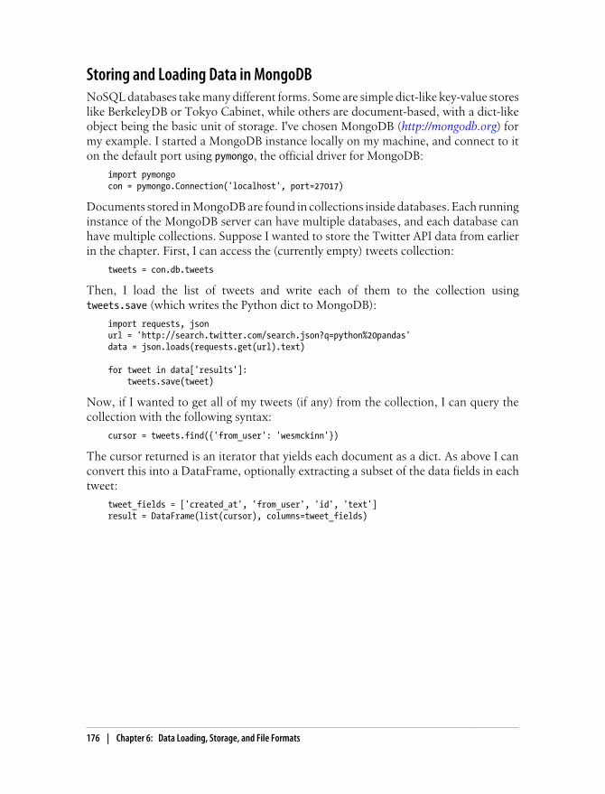
Storing and Loading Data in MongoDBNoSQL databases take many different forms. Some are simple dict-like key-value storeslike BerkeleyDB or Tokyo Cabinet, while others are document-based, with a dict-likeobject being the basic unit of storage. I've chosen MongoDB (http://mongodb.org) formy example. I started a MongoDB instance locally on my machine, and connect to iton the default port using pymongo, the official driver for MongoDB:
import pymongocon = pymongo.Connection('localhost', port=27017)
Documents stored in MongoDB are found in collections inside databases. Each runninginstance of the MongoDB server can have multiple databases, and each database canhave multiple collections. Suppose I wanted to store the Twitter API data from earlierin the chapter. First, I can access the (currently empty) tweets collection:
tweets = con.db.tweets
Then, I load the list of tweets and write each of them to the collection usingtweets.save (which writes the Python dict to MongoDB):
import requests, jsonurl = 'http://search.twitter.com/search.json?q=python%20pandas'data = json.loads(requests.get(url).text)
for tweet in data['results']: tweets.save(tweet)
Now, if I wanted to get all of my tweets (if any) from the collection, I can query thecollection with the following syntax:
cursor = tweets.find({'from_user': 'wesmckinn'})
The cursor returned is an iterator that yields each document as a dict. As above I canconvert this into a DataFrame, optionally extracting a subset of the data fields in eachtweet:
tweet_fields = ['created_at', 'from_user', 'id', 'text']result = DataFrame(list(cursor), columns=tweet_fields)
176 | Chapter 6: Data Loading, Storage, and File Formats
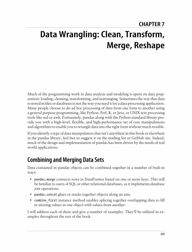
CHAPTER 7
Data Wrangling: Clean, Transform,Merge, Reshape
Much of the programming work in data analysis and modeling is spent on data prep-aration: loading, cleaning, transforming, and rearranging. Sometimes the way that datais stored in files or databases is not the way you need it for a data processing application.Many people choose to do ad hoc processing of data from one form to another usinga general purpose programming, like Python, Perl, R, or Java, or UNIX text processingtools like sed or awk. Fortunately, pandas along with the Python standard library pro-vide you with a high-level, flexible, and high-performance set of core manipulationsand algorithms to enable you to wrangle data into the right form without much trouble.
If you identify a type of data manipulation that isn’t anywhere in this book or elsewherein the pandas library, feel free to suggest it on the mailing list or GitHub site. Indeed,much of the design and implementation of pandas has been driven by the needs of realworld applications.
Combining and Merging Data SetsData contained in pandas objects can be combined together in a number of built-inways:
• pandas.merge connects rows in DataFrames based on one or more keys. This willbe familiar to users of SQL or other relational databases, as it implements databasejoin operations.
• pandas.concat glues or stacks together objects along an axis.
• combine_first instance method enables splicing together overlapping data to fillin missing values in one object with values from another.
I will address each of these and give a number of examples. They’ll be utilized in ex-amples throughout the rest of the book.
177

Database-style DataFrame MergesMerge or join operations combine data sets by linking rows using one or more keys.These operations are central to relational databases. The merge function in pandas isthe main entry point for using these algorithms on your data.
Let’s start with a simple example:
In [15]: df1 = DataFrame({'key': ['b', 'b', 'a', 'c', 'a', 'a', 'b'], ....: 'data1': range(7)})
In [16]: df2 = DataFrame({'key': ['a', 'b', 'd'], ....: 'data2': range(3)})
In [17]: df1 In [18]: df2Out[17]: Out[18]: data1 key data2 key0 0 b 0 0 a1 1 b 1 1 b2 2 a 2 2 d3 3 c4 4 a5 5 a6 6 b
This is an example of a many-to-one merge situation; the data in df1 has multiple rowslabeled a and b, whereas df2 has only one row for each value in the key column. Callingmerge with these objects we obtain:
In [19]: pd.merge(df1, df2)Out[19]: data1 key data20 2 a 01 4 a 02 5 a 03 0 b 14 1 b 15 6 b 1
Note that I didn’t specify which column to join on. If not specified, merge uses theoverlapping column names as the keys. It’s a good practice to specify explicitly, though:
In [20]: pd.merge(df1, df2, on='key')Out[20]: data1 key data20 2 a 01 4 a 02 5 a 03 0 b 14 1 b 15 6 b 1
If the column names are different in each object, you can specify them separately:
In [21]: df3 = DataFrame({'lkey': ['b', 'b', 'a', 'c', 'a', 'a', 'b'], ....: 'data1': range(7)})
178 | Chapter 7: Data Wrangling: Clean, Transform, Merge, Reshape

In [22]: df4 = DataFrame({'rkey': ['a', 'b', 'd'], ....: 'data2': range(3)})
In [23]: pd.merge(df3, df4, left_on='lkey', right_on='rkey')Out[23]: data1 lkey data2 rkey0 2 a 0 a1 4 a 0 a2 5 a 0 a3 0 b 1 b4 1 b 1 b5 6 b 1 b
You probably noticed that the 'c' and 'd' values and associated data are missing fromthe result. By default merge does an 'inner' join; the keys in the result are the intersec-tion. Other possible options are 'left', 'right', and 'outer'. The outer join takes theunion of the keys, combining the effect of applying both left and right joins:
In [24]: pd.merge(df1, df2, how='outer')Out[24]: data1 key data20 2 a 01 4 a 02 5 a 03 0 b 14 1 b 15 6 b 16 3 c NaN7 NaN d 2
Many-to-many merges have well-defined though not necessarily intuitive behavior.Here’s an example:
In [25]: df1 = DataFrame({'key': ['b', 'b', 'a', 'c', 'a', 'b'], ....: 'data1': range(6)})
In [26]: df2 = DataFrame({'key': ['a', 'b', 'a', 'b', 'd'], ....: 'data2': range(5)})
In [27]: df1 In [28]: df2Out[27]: Out[28]: data1 key data2 key0 0 b 0 0 a1 1 b 1 1 b2 2 a 2 2 a3 3 c 3 3 b4 4 a 4 4 d5 5 b
In [29]: pd.merge(df1, df2, on='key', how='left')Out[29]: data1 key data20 2 a 01 2 a 2
Combining and Merging Data Sets | 179

2 4 a 03 4 a 24 0 b 15 0 b 36 1 b 17 1 b 38 5 b 19 5 b 310 3 c NaN
Many-to-many joins form the Cartesian product of the rows. Since there were 3 'b'rows in the left DataFrame and 2 in the right one, there are 6 'b' rows in the result.The join method only affects the distinct key values appearing in the result:
In [30]: pd.merge(df1, df2, how='inner')Out[30]: data1 key data20 2 a 01 2 a 22 4 a 03 4 a 24 0 b 15 0 b 36 1 b 17 1 b 38 5 b 19 5 b 3
To merge with multiple keys, pass a list of column names:
In [31]: left = DataFrame({'key1': ['foo', 'foo', 'bar'], ....: 'key2': ['one', 'two', 'one'], ....: 'lval': [1, 2, 3]})
In [32]: right = DataFrame({'key1': ['foo', 'foo', 'bar', 'bar'], ....: 'key2': ['one', 'one', 'one', 'two'], ....: 'rval': [4, 5, 6, 7]})
In [33]: pd.merge(left, right, on=['key1', 'key2'], how='outer')Out[33]: key1 key2 lval rval0 bar one 3 61 bar two NaN 72 foo one 1 43 foo one 1 54 foo two 2 NaN
To determine which key combinations will appear in the result depending on the choiceof merge method, think of the multiple keys as forming an array of tuples to be usedas a single join key (even though it’s not actually implemented that way).
When joining columns-on-columns, the indexes on the passed Data-Frame objects are discarded.
180 | Chapter 7: Data Wrangling: Clean, Transform, Merge, Reshape
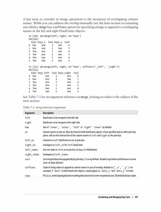
A last issue to consider in merge operations is the treatment of overlapping columnnames. While you can address the overlap manually (see the later section on renamingaxis labels), merge has a suffixes option for specifying strings to append to overlappingnames in the left and right DataFrame objects:
In [34]: pd.merge(left, right, on='key1')Out[34]: key1 key2_x lval key2_y rval0 bar one 3 one 61 bar one 3 two 72 foo one 1 one 43 foo one 1 one 54 foo two 2 one 45 foo two 2 one 5
In [35]: pd.merge(left, right, on='key1', suffixes=('_left', '_right'))Out[35]: key1 key2_left lval key2_right rval0 bar one 3 one 61 bar one 3 two 72 foo one 1 one 43 foo one 1 one 54 foo two 2 one 45 foo two 2 one 5
See Table 7-1 for an argument reference on merge. Joining on index is the subject of thenext section.
Table 7-1. merge function arguments
Argument Description
left DataFrame to be merged on the left side
right DataFrame to be merged on the right side
how One of 'inner', 'outer', 'left' or 'right'. 'inner' by default
on Column names to join on. Must be found in both DataFrame objects. If not specified and no other join keysgiven, will use the intersection of the column names in left and right as the join keys
left_on Columns in left DataFrame to use as join keys
right_on Analogous to left_on for left DataFrame
left_index Use row index in left as its join key (or keys, if a MultiIndex)
right_index Analogous to left_index
sort Sort merged data lexicographically by join keys; True by default. Disable to get better performance in somecases on large datasets
suffixes Tuple of string values to append to column names in case of overlap; defaults to ('_x', '_y'). Forexample, if 'data' in both DataFrame objects, would appear as 'data_x' and 'data_y' in result
copy If False, avoid copying data into resulting data structure in some exceptional cases. By default always copies
Combining and Merging Data Sets | 181

Merging on IndexIn some cases, the merge key or keys in a DataFrame will be found in its index. In thiscase, you can pass left_index=True or right_index=True (or both) to indicate that theindex should be used as the merge key:
In [36]: left1 = DataFrame({'key': ['a', 'b', 'a', 'a', 'b', 'c'], ....: 'value': range(6)})
In [37]: right1 = DataFrame({'group_val': [3.5, 7]}, index=['a', 'b'])
In [38]: left1 In [39]: right1Out[38]: Out[39]: key value group_val0 a 0 a 3.51 b 1 b 7.02 a 23 a 34 b 45 c 5
In [40]: pd.merge(left1, right1, left_on='key', right_index=True)Out[40]: key value group_val0 a 0 3.52 a 2 3.53 a 3 3.51 b 1 7.04 b 4 7.0
Since the default merge method is to intersect the join keys, you can instead form theunion of them with an outer join:
In [41]: pd.merge(left1, right1, left_on='key', right_index=True, how='outer')Out[41]: key value group_val0 a 0 3.52 a 2 3.53 a 3 3.51 b 1 7.04 b 4 7.05 c 5 NaN
With hierarchically-indexed data, things are a bit more complicated:
In [42]: lefth = DataFrame({'key1': ['Ohio', 'Ohio', 'Ohio', 'Nevada', 'Nevada'], ....: 'key2': [2000, 2001, 2002, 2001, 2002], ....: 'data': np.arange(5.)})
In [43]: righth = DataFrame(np.arange(12).reshape((6, 2)), ....: index=[['Nevada', 'Nevada', 'Ohio', 'Ohio', 'Ohio', 'Ohio'], ....: [2001, 2000, 2000, 2000, 2001, 2002]], ....: columns=['event1', 'event2'])
In [44]: lefth In [45]: righthOut[44]: Out[45]:
182 | Chapter 7: Data Wrangling: Clean, Transform, Merge, Reshape

data key1 key2 event1 event20 0 Ohio 2000 Nevada 2001 0 11 1 Ohio 2001 2000 2 32 2 Ohio 2002 Ohio 2000 4 53 3 Nevada 2001 2000 6 74 4 Nevada 2002 2001 8 9 2002 10 11
In this case, you have to indicate multiple columns to merge on as a list (pay attentionto the handling of duplicate index values):
In [46]: pd.merge(lefth, righth, left_on=['key1', 'key2'], right_index=True)Out[46]: data key1 key2 event1 event23 3 Nevada 2001 0 10 0 Ohio 2000 4 50 0 Ohio 2000 6 71 1 Ohio 2001 8 92 2 Ohio 2002 10 11
In [47]: pd.merge(lefth, righth, left_on=['key1', 'key2'], ....: right_index=True, how='outer')Out[47]: data key1 key2 event1 event24 NaN Nevada 2000 2 33 3 Nevada 2001 0 14 4 Nevada 2002 NaN NaN0 0 Ohio 2000 4 50 0 Ohio 2000 6 71 1 Ohio 2001 8 92 2 Ohio 2002 10 11
Using the indexes of both sides of the merge is also not an issue:
In [48]: left2 = DataFrame([[1., 2.], [3., 4.], [5., 6.]], index=['a', 'c', 'e'], ....: columns=['Ohio', 'Nevada'])
In [49]: right2 = DataFrame([[7., 8.], [9., 10.], [11., 12.], [13, 14]], ....: index=['b', 'c', 'd', 'e'], columns=['Missouri', 'Alabama'])
In [50]: left2 In [51]: right2Out[50]: Out[51]: Ohio Nevada Missouri Alabamaa 1 2 b 7 8c 3 4 c 9 10e 5 6 d 11 12 e 13 14
In [52]: pd.merge(left2, right2, how='outer', left_index=True, right_index=True)Out[52]: Ohio Nevada Missouri Alabamaa 1 2 NaN NaNb NaN NaN 7 8c 3 4 9 10d NaN NaN 11 12e 5 6 13 14
Combining and Merging Data Sets | 183
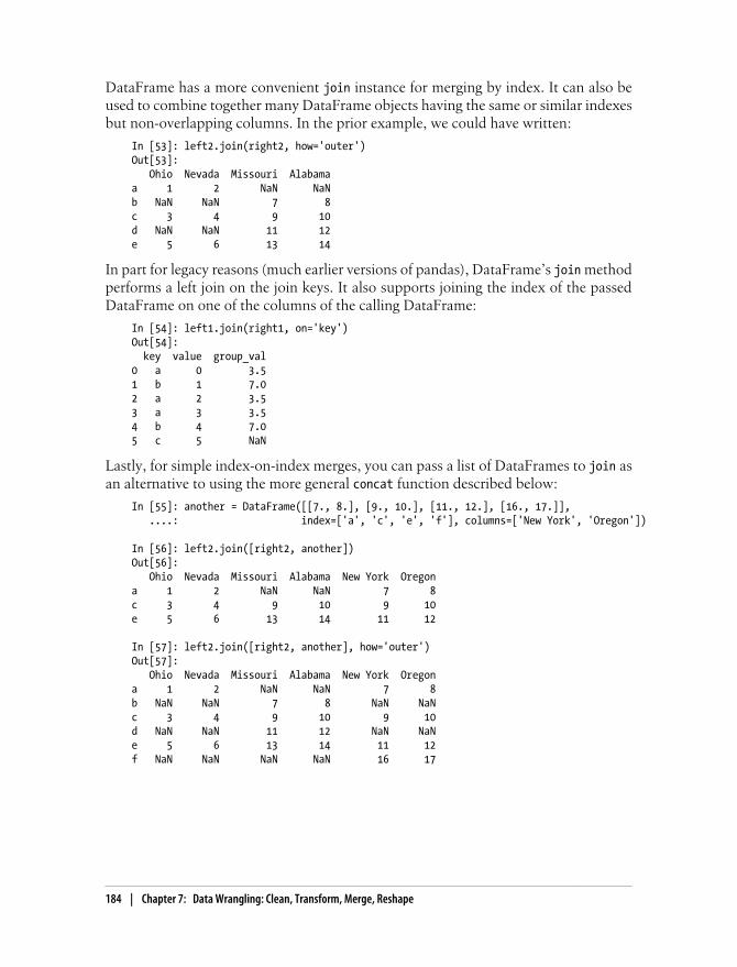
DataFrame has a more convenient join instance for merging by index. It can also beused to combine together many DataFrame objects having the same or similar indexesbut non-overlapping columns. In the prior example, we could have written:
In [53]: left2.join(right2, how='outer')Out[53]: Ohio Nevada Missouri Alabamaa 1 2 NaN NaNb NaN NaN 7 8c 3 4 9 10d NaN NaN 11 12e 5 6 13 14
In part for legacy reasons (much earlier versions of pandas), DataFrame’s join methodperforms a left join on the join keys. It also supports joining the index of the passedDataFrame on one of the columns of the calling DataFrame:
In [54]: left1.join(right1, on='key')Out[54]: key value group_val0 a 0 3.51 b 1 7.02 a 2 3.53 a 3 3.54 b 4 7.05 c 5 NaN
Lastly, for simple index-on-index merges, you can pass a list of DataFrames to join asan alternative to using the more general concat function described below:
In [55]: another = DataFrame([[7., 8.], [9., 10.], [11., 12.], [16., 17.]], ....: index=['a', 'c', 'e', 'f'], columns=['New York', 'Oregon'])
In [56]: left2.join([right2, another])Out[56]: Ohio Nevada Missouri Alabama New York Oregona 1 2 NaN NaN 7 8c 3 4 9 10 9 10e 5 6 13 14 11 12
In [57]: left2.join([right2, another], how='outer')Out[57]: Ohio Nevada Missouri Alabama New York Oregona 1 2 NaN NaN 7 8b NaN NaN 7 8 NaN NaNc 3 4 9 10 9 10d NaN NaN 11 12 NaN NaNe 5 6 13 14 11 12f NaN NaN NaN NaN 16 17
184 | Chapter 7: Data Wrangling: Clean, Transform, Merge, Reshape

Concatenating Along an AxisAnother kind of data combination operation is alternatively referred to as concatena-tion, binding, or stacking. NumPy has a concatenate function for doing this with rawNumPy arrays:
In [58]: arr = np.arange(12).reshape((3, 4))
In [59]: arrOut[59]:array([[ 0, 1, 2, 3], [ 4, 5, 6, 7], [ 8, 9, 10, 11]])
In [60]: np.concatenate([arr, arr], axis=1)Out[60]:array([[ 0, 1, 2, 3, 0, 1, 2, 3], [ 4, 5, 6, 7, 4, 5, 6, 7], [ 8, 9, 10, 11, 8, 9, 10, 11]])
In the context of pandas objects such as Series and DataFrame, having labeled axesenable you to further generalize array concatenation. In particular, you have a numberof additional things to think about:
• If the objects are indexed differently on the other axes, should the collection ofaxes be unioned or intersected?
• Do the groups need to be identifiable in the resulting object?
• Does the concatenation axis matter at all?
The concat function in pandas provides a consistent way to address each of these con-cerns. I’ll give a number of examples to illustrate how it works. Suppose we have threeSeries with no index overlap:
In [61]: s1 = Series([0, 1], index=['a', 'b'])
In [62]: s2 = Series([2, 3, 4], index=['c', 'd', 'e'])
In [63]: s3 = Series([5, 6], index=['f', 'g'])
Calling concat with these object in a list glues together the values and indexes:
In [64]: pd.concat([s1, s2, s3])Out[64]:a 0b 1c 2d 3e 4f 5g 6
Combining and Merging Data Sets | 185
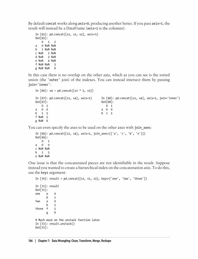
By default concat works along axis=0, producing another Series. If you pass axis=1, theresult will instead be a DataFrame (axis=1 is the columns):
In [65]: pd.concat([s1, s2, s3], axis=1)Out[65]: 0 1 2a 0 NaN NaNb 1 NaN NaNc NaN 2 NaNd NaN 3 NaNe NaN 4 NaNf NaN NaN 5g NaN NaN 6
In this case there is no overlap on the other axis, which as you can see is the sortedunion (the 'outer' join) of the indexes. You can instead intersect them by passingjoin='inner':
In [66]: s4 = pd.concat([s1 * 5, s3])
In [67]: pd.concat([s1, s4], axis=1) In [68]: pd.concat([s1, s4], axis=1, join='inner')Out[67]: Out[68]: 0 1 0 1a 0 0 a 0 0b 1 5 b 1 5f NaN 5g NaN 6
You can even specify the axes to be used on the other axes with join_axes:
In [69]: pd.concat([s1, s4], axis=1, join_axes=[['a', 'c', 'b', 'e']])Out[69]: 0 1a 0 0c NaN NaNb 1 5e NaN NaN
One issue is that the concatenated pieces are not identifiable in the result. Supposeinstead you wanted to create a hierarchical index on the concatenation axis. To do this,use the keys argument:
In [70]: result = pd.concat([s1, s1, s3], keys=['one', 'two', 'three'])
In [71]: resultOut[71]:one a 0 b 1two a 0 b 1three f 5 g 6
# Much more on the unstack function laterIn [72]: result.unstack()Out[72]:
186 | Chapter 7: Data Wrangling: Clean, Transform, Merge, Reshape

a b f gone 0 1 NaN NaNtwo 0 1 NaN NaNthree NaN NaN 5 6
In the case of combining Series along axis=1, the keys become the DataFrame columnheaders:
In [73]: pd.concat([s1, s2, s3], axis=1, keys=['one', 'two', 'three'])Out[73]: one two threea 0 NaN NaNb 1 NaN NaNc NaN 2 NaNd NaN 3 NaNe NaN 4 NaNf NaN NaN 5g NaN NaN 6
The same logic extends to DataFrame objects:
In [74]: df1 = DataFrame(np.arange(6).reshape(3, 2), index=['a', 'b', 'c'], ....: columns=['one', 'two'])
In [75]: df2 = DataFrame(5 + np.arange(4).reshape(2, 2), index=['a', 'c'], ....: columns=['three', 'four'])
In [76]: pd.concat([df1, df2], axis=1, keys=['level1', 'level2'])Out[76]: level1 level2 one two three foura 0 1 5 6b 2 3 NaN NaNc 4 5 7 8
If you pass a dict of objects instead of a list, the dict’s keys will be used for the keysoption:
In [77]: pd.concat({'level1': df1, 'level2': df2}, axis=1)Out[77]: level1 level2 one two three foura 0 1 5 6b 2 3 NaN NaNc 4 5 7 8
There are a couple of additional arguments governing how the hierarchical index iscreated (see Table 7-2):
In [78]: pd.concat([df1, df2], axis=1, keys=['level1', 'level2'], ....: names=['upper', 'lower'])Out[78]:upper level1 level2lower one two three foura 0 1 5 6b 2 3 NaN NaNc 4 5 7 8
Combining and Merging Data Sets | 187

A last consideration concerns DataFrames in which the row index is not meaningful inthe context of the analysis:
In [79]: df1 = DataFrame(np.random.randn(3, 4), columns=['a', 'b', 'c', 'd'])
In [80]: df2 = DataFrame(np.random.randn(2, 3), columns=['b', 'd', 'a'])
In [81]: df1 In [82]: df2Out[81]: Out[82]: a b c d b d a0 -0.204708 0.478943 -0.519439 -0.555730 0 0.274992 0.228913 1.3529171 1.965781 1.393406 0.092908 0.281746 1 0.886429 -2.001637 -0.3718432 0.769023 1.246435 1.007189 -1.296221
In this case, you can pass ignore_index=True:
In [83]: pd.concat([df1, df2], ignore_index=True)Out[83]: a b c d0 -0.204708 0.478943 -0.519439 -0.5557301 1.965781 1.393406 0.092908 0.2817462 0.769023 1.246435 1.007189 -1.2962213 1.352917 0.274992 NaN 0.2289134 -0.371843 0.886429 NaN -2.001637
Table 7-2. concat function arguments
Argument Description
objs List or dict of pandas objects to be concatenated. The only required argument
axis Axis to concatenate along; defaults to 0
join One of 'inner', 'outer', defaulting to 'outer'; whether to intersection (inner) or union(outer) together indexes along the other axes
join_axes Specific indexes to use for the other n-1 axes instead of performing union/intersection logic
keys Values to associate with objects being concatenated, forming a hierarchical index along theconcatenation axis. Can either be a list or array of arbitrary values, an array of tuples, or a list ofarrays (if multiple level arrays passed in levels)
levels Specific indexes to use as hierarchical index level or levels if keys passed
names Names for created hierarchical levels if keys and / or levels passed
verify_integrity Check new axis in concatenated object for duplicates and raise exception if so. By default(False) allows duplicates
ignore_index Do not preserve indexes along concatenation axis, instead producing a newrange(total_length) index
Combining Data with OverlapAnother data combination situation can’t be expressed as either a merge or concate-nation operation. You may have two datasets whose indexes overlap in full or part. Asa motivating example, consider NumPy’s where function, which expressed a vectorizedif-else:
188 | Chapter 7: Data Wrangling: Clean, Transform, Merge, Reshape
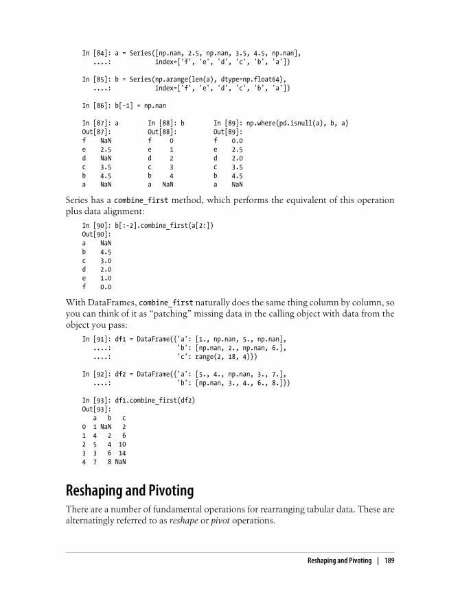
In [84]: a = Series([np.nan, 2.5, np.nan, 3.5, 4.5, np.nan], ....: index=['f', 'e', 'd', 'c', 'b', 'a'])
In [85]: b = Series(np.arange(len(a), dtype=np.float64), ....: index=['f', 'e', 'd', 'c', 'b', 'a'])
In [86]: b[-1] = np.nan
In [87]: a In [88]: b In [89]: np.where(pd.isnull(a), b, a)Out[87]: Out[88]: Out[89]:f NaN f 0 f 0.0e 2.5 e 1 e 2.5d NaN d 2 d 2.0c 3.5 c 3 c 3.5b 4.5 b 4 b 4.5a NaN a NaN a NaN
Series has a combine_first method, which performs the equivalent of this operationplus data alignment:
In [90]: b[:-2].combine_first(a[2:])Out[90]:a NaNb 4.5c 3.0d 2.0e 1.0f 0.0
With DataFrames, combine_first naturally does the same thing column by column, soyou can think of it as “patching” missing data in the calling object with data from theobject you pass:
In [91]: df1 = DataFrame({'a': [1., np.nan, 5., np.nan], ....: 'b': [np.nan, 2., np.nan, 6.], ....: 'c': range(2, 18, 4)})
In [92]: df2 = DataFrame({'a': [5., 4., np.nan, 3., 7.], ....: 'b': [np.nan, 3., 4., 6., 8.]})
In [93]: df1.combine_first(df2)Out[93]: a b c0 1 NaN 21 4 2 62 5 4 103 3 6 144 7 8 NaN
Reshaping and PivotingThere are a number of fundamental operations for rearranging tabular data. These arealternatingly referred to as reshape or pivot operations.
Reshaping and Pivoting | 189

Reshaping with Hierarchical IndexingHierarchical indexing provides a consistent way to rearrange data in a DataFrame.There are two primary actions:
• stack: this “rotates” or pivots from the columns in the data to the rows
• unstack: this pivots from the rows into the columns
I’ll illustrate these operations through a series of examples. Consider a small DataFramewith string arrays as row and column indexes:
In [94]: data = DataFrame(np.arange(6).reshape((2, 3)), ....: index=pd.Index(['Ohio', 'Colorado'], name='state'), ....: columns=pd.Index(['one', 'two', 'three'], name='number'))
In [95]: dataOut[95]:number one two threestateOhio 0 1 2Colorado 3 4 5
Using the stack method on this data pivots the columns into the rows, producing aSeries:
In [96]: result = data.stack()
In [97]: resultOut[97]:state numberOhio one 0 two 1 three 2Colorado one 3 two 4 three 5
From a hierarchically-indexed Series, you can rearrange the data back into a DataFramewith unstack:
In [98]: result.unstack()Out[98]:number one two threestateOhio 0 1 2Colorado 3 4 5
By default the innermost level is unstacked (same with stack). You can unstack a dif-ferent level by passing a level number or name:
In [99]: result.unstack(0) In [100]: result.unstack('state')Out[99]: Out[100]:state Ohio Colorado state Ohio Coloradonumber numberone 0 3 one 0 3
190 | Chapter 7: Data Wrangling: Clean, Transform, Merge, Reshape
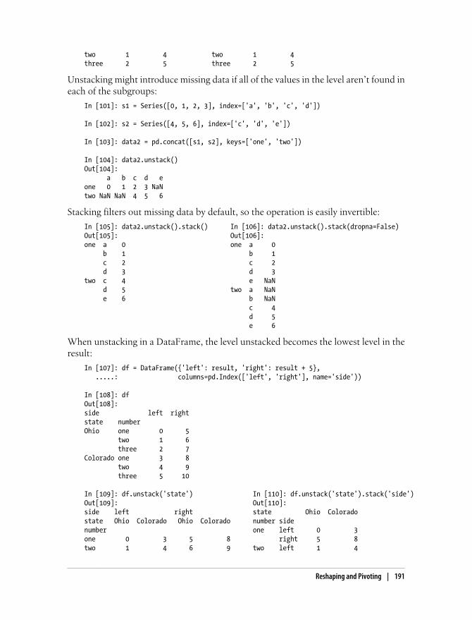
two 1 4 two 1 4three 2 5 three 2 5
Unstacking might introduce missing data if all of the values in the level aren’t found ineach of the subgroups:
In [101]: s1 = Series([0, 1, 2, 3], index=['a', 'b', 'c', 'd'])
In [102]: s2 = Series([4, 5, 6], index=['c', 'd', 'e'])
In [103]: data2 = pd.concat([s1, s2], keys=['one', 'two'])
In [104]: data2.unstack()Out[104]: a b c d eone 0 1 2 3 NaNtwo NaN NaN 4 5 6
Stacking filters out missing data by default, so the operation is easily invertible:
In [105]: data2.unstack().stack() In [106]: data2.unstack().stack(dropna=False)Out[105]: Out[106]:one a 0 one a 0 b 1 b 1 c 2 c 2 d 3 d 3two c 4 e NaN d 5 two a NaN e 6 b NaN c 4 d 5 e 6
When unstacking in a DataFrame, the level unstacked becomes the lowest level in theresult:
In [107]: df = DataFrame({'left': result, 'right': result + 5}, .....: columns=pd.Index(['left', 'right'], name='side'))
In [108]: dfOut[108]:side left rightstate numberOhio one 0 5 two 1 6 three 2 7Colorado one 3 8 two 4 9 three 5 10
In [109]: df.unstack('state') In [110]: df.unstack('state').stack('side')Out[109]: Out[110]:side left right state Ohio Coloradostate Ohio Colorado Ohio Colorado number sidenumber one left 0 3one 0 3 5 8 right 5 8two 1 4 6 9 two left 1 4
Reshaping and Pivoting | 191

three 2 5 7 10 right 6 9 three left 2 5 right 7 10
Pivoting “long” to “wide” FormatA common way to store multiple time series in databases and CSV is in so-called longor stacked format:
In [116]: ldata[:10]Out[116]: date item value0 1959-03-31 00:00:00 realgdp 2710.3491 1959-03-31 00:00:00 infl 0.0002 1959-03-31 00:00:00 unemp 5.8003 1959-06-30 00:00:00 realgdp 2778.8014 1959-06-30 00:00:00 infl 2.3405 1959-06-30 00:00:00 unemp 5.1006 1959-09-30 00:00:00 realgdp 2775.4887 1959-09-30 00:00:00 infl 2.7408 1959-09-30 00:00:00 unemp 5.3009 1959-12-31 00:00:00 realgdp 2785.204
Data is frequently stored this way in relational databases like MySQL as a fixed schema(column names and data types) allows the number of distinct values in the item columnto increase or decrease as data is added or deleted in the table. In the above exampledate and item would usually be the primary keys (in relational database parlance),offering both relational integrity and easier joins and programmatic queries in manycases. The downside, of course, is that the data may not be easy to work with in longformat; you might prefer to have a DataFrame containing one column per distinctitem value indexed by timestamps in the date column. DataFrame’s pivot method per-forms exactly this transformation:
In [117]: pivoted = ldata.pivot('date', 'item', 'value')
In [118]: pivoted.head()Out[118]:item infl realgdp unempdate1959-03-31 0.00 2710.349 5.81959-06-30 2.34 2778.801 5.11959-09-30 2.74 2775.488 5.31959-12-31 0.27 2785.204 5.61960-03-31 2.31 2847.699 5.2
The first two values passed are the columns to be used as the row and column index,and finally an optional value column to fill the DataFrame. Suppose you had two valuecolumns that you wanted to reshape simultaneously:
In [119]: ldata['value2'] = np.random.randn(len(ldata))
In [120]: ldata[:10]Out[120]:
192 | Chapter 7: Data Wrangling: Clean, Transform, Merge, Reshape
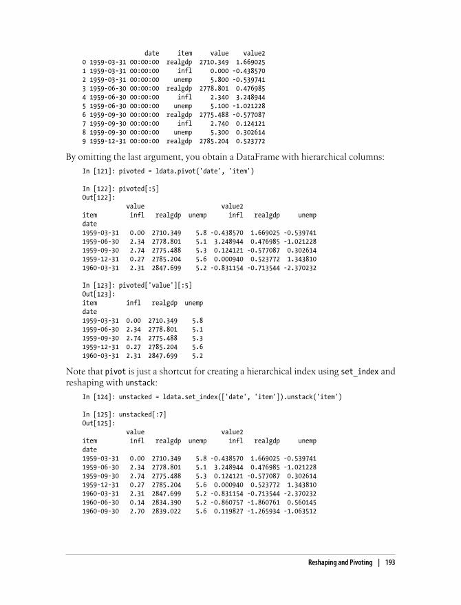
date item value value20 1959-03-31 00:00:00 realgdp 2710.349 1.6690251 1959-03-31 00:00:00 infl 0.000 -0.4385702 1959-03-31 00:00:00 unemp 5.800 -0.5397413 1959-06-30 00:00:00 realgdp 2778.801 0.4769854 1959-06-30 00:00:00 infl 2.340 3.2489445 1959-06-30 00:00:00 unemp 5.100 -1.0212286 1959-09-30 00:00:00 realgdp 2775.488 -0.5770877 1959-09-30 00:00:00 infl 2.740 0.1241218 1959-09-30 00:00:00 unemp 5.300 0.3026149 1959-12-31 00:00:00 realgdp 2785.204 0.523772
By omitting the last argument, you obtain a DataFrame with hierarchical columns:
In [121]: pivoted = ldata.pivot('date', 'item')
In [122]: pivoted[:5]Out[122]: value value2item infl realgdp unemp infl realgdp unempdate1959-03-31 0.00 2710.349 5.8 -0.438570 1.669025 -0.5397411959-06-30 2.34 2778.801 5.1 3.248944 0.476985 -1.0212281959-09-30 2.74 2775.488 5.3 0.124121 -0.577087 0.3026141959-12-31 0.27 2785.204 5.6 0.000940 0.523772 1.3438101960-03-31 2.31 2847.699 5.2 -0.831154 -0.713544 -2.370232
In [123]: pivoted['value'][:5]Out[123]:item infl realgdp unempdate1959-03-31 0.00 2710.349 5.81959-06-30 2.34 2778.801 5.11959-09-30 2.74 2775.488 5.31959-12-31 0.27 2785.204 5.61960-03-31 2.31 2847.699 5.2
Note that pivot is just a shortcut for creating a hierarchical index using set_index andreshaping with unstack:
In [124]: unstacked = ldata.set_index(['date', 'item']).unstack('item')
In [125]: unstacked[:7]Out[125]: value value2item infl realgdp unemp infl realgdp unempdate1959-03-31 0.00 2710.349 5.8 -0.438570 1.669025 -0.5397411959-06-30 2.34 2778.801 5.1 3.248944 0.476985 -1.0212281959-09-30 2.74 2775.488 5.3 0.124121 -0.577087 0.3026141959-12-31 0.27 2785.204 5.6 0.000940 0.523772 1.3438101960-03-31 2.31 2847.699 5.2 -0.831154 -0.713544 -2.3702321960-06-30 0.14 2834.390 5.2 -0.860757 -1.860761 0.5601451960-09-30 2.70 2839.022 5.6 0.119827 -1.265934 -1.063512
Reshaping and Pivoting | 193

Data TransformationSo far in this chapter we’ve been concerned with rearranging data. Filtering, cleaning,and other tranformations are another class of important operations.
Removing DuplicatesDuplicate rows may be found in a DataFrame for any number of reasons. Here is anexample:
In [126]: data = DataFrame({'k1': ['one'] * 3 + ['two'] * 4, .....: 'k2': [1, 1, 2, 3, 3, 4, 4]})
In [127]: dataOut[127]: k1 k20 one 11 one 12 one 23 two 34 two 35 two 46 two 4
The DataFrame method duplicated returns a boolean Series indicating whether eachrow is a duplicate or not:
In [128]: data.duplicated()Out[128]:0 False1 True2 False3 False4 True5 False6 True
Relatedly, drop_duplicates returns a DataFrame where the duplicated array is True:
In [129]: data.drop_duplicates()Out[129]: k1 k20 one 12 one 23 two 35 two 4
Both of these methods by default consider all of the columns; alternatively you canspecify any subset of them to detect duplicates. Suppose we had an additional columnof values and wanted to filter duplicates only based on the 'k1' column:
In [130]: data['v1'] = range(7)
In [131]: data.drop_duplicates(['k1'])
194 | Chapter 7: Data Wrangling: Clean, Transform, Merge, Reshape
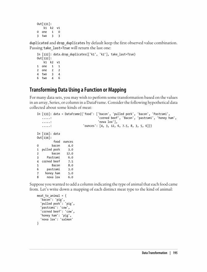
Out[131]: k1 k2 v10 one 1 03 two 3 3
duplicated and drop_duplicates by default keep the first observed value combination.Passing take_last=True will return the last one:
In [132]: data.drop_duplicates(['k1', 'k2'], take_last=True)Out[132]: k1 k2 v11 one 1 12 one 2 24 two 3 46 two 4 6
Transforming Data Using a Function or MappingFor many data sets, you may wish to perform some transformation based on the valuesin an array, Series, or column in a DataFrame. Consider the following hypothetical datacollected about some kinds of meat:
In [133]: data = DataFrame({'food': ['bacon', 'pulled pork', 'bacon', 'Pastrami', .....: 'corned beef', 'Bacon', 'pastrami', 'honey ham', .....: 'nova lox'], .....: 'ounces': [4, 3, 12, 6, 7.5, 8, 3, 5, 6]})
In [134]: dataOut[134]: food ounces0 bacon 4.01 pulled pork 3.02 bacon 12.03 Pastrami 6.04 corned beef 7.55 Bacon 8.06 pastrami 3.07 honey ham 5.08 nova lox 6.0
Suppose you wanted to add a column indicating the type of animal that each food camefrom. Let’s write down a mapping of each distinct meat type to the kind of animal:
meat_to_animal = { 'bacon': 'pig', 'pulled pork': 'pig', 'pastrami': 'cow', 'corned beef': 'cow', 'honey ham': 'pig', 'nova lox': 'salmon'}
Data Transformation | 195
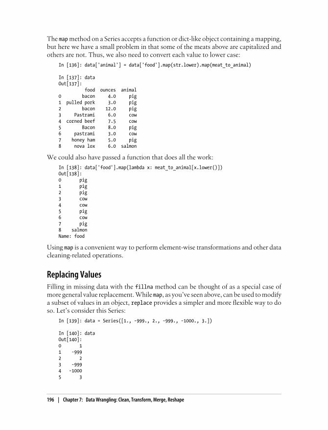
The map method on a Series accepts a function or dict-like object containing a mapping,but here we have a small problem in that some of the meats above are capitalized andothers are not. Thus, we also need to convert each value to lower case:
In [136]: data['animal'] = data['food'].map(str.lower).map(meat_to_animal)
In [137]: dataOut[137]: food ounces animal0 bacon 4.0 pig1 pulled pork 3.0 pig2 bacon 12.0 pig3 Pastrami 6.0 cow4 corned beef 7.5 cow5 Bacon 8.0 pig6 pastrami 3.0 cow7 honey ham 5.0 pig8 nova lox 6.0 salmon
We could also have passed a function that does all the work:
In [138]: data['food'].map(lambda x: meat_to_animal[x.lower()])Out[138]:0 pig1 pig2 pig3 cow4 cow5 pig6 cow7 pig8 salmonName: food
Using map is a convenient way to perform element-wise transformations and other datacleaning-related operations.
Replacing ValuesFilling in missing data with the fillna method can be thought of as a special case ofmore general value replacement. While map, as you’ve seen above, can be used to modifya subset of values in an object, replace provides a simpler and more flexible way to doso. Let’s consider this Series:
In [139]: data = Series([1., -999., 2., -999., -1000., 3.])
In [140]: dataOut[140]:0 11 -9992 23 -9994 -10005 3
196 | Chapter 7: Data Wrangling: Clean, Transform, Merge, Reshape

The -999 values might be sentinel values for missing data. To replace these with NAvalues that pandas understands, we can use replace, producing a new Series:
In [141]: data.replace(-999, np.nan)Out[141]:0 11 NaN2 23 NaN4 -10005 3
If you want to replace multiple values at once, you instead pass a list then the substitutevalue:
In [142]: data.replace([-999, -1000], np.nan)Out[142]:0 11 NaN2 23 NaN4 NaN5 3
To use a different replacement for each value, pass a list of substitutes:
In [143]: data.replace([-999, -1000], [np.nan, 0])Out[143]:0 11 NaN2 23 NaN4 05 3
The argument passed can also be a dict:
In [144]: data.replace({-999: np.nan, -1000: 0})Out[144]:0 11 NaN2 23 NaN4 05 3
Renaming Axis IndexesLike values in a Series, axis labels can be similarly transformed by a function or mappingof some form to produce new, differently labeled objects. The axes can also be modifiedin place without creating a new data structure. Here’s a simple example:
In [145]: data = DataFrame(np.arange(12).reshape((3, 4)), .....: index=['Ohio', 'Colorado', 'New York'], .....: columns=['one', 'two', 'three', 'four'])
Data Transformation | 197

Like a Series, the axis indexes have a map method:
In [146]: data.index.map(str.upper)Out[146]: array([OHIO, COLORADO, NEW YORK], dtype=object)
You can assign to index, modifying the DataFrame in place:
In [147]: data.index = data.index.map(str.upper)
In [148]: dataOut[148]: one two three fourOHIO 0 1 2 3COLORADO 4 5 6 7NEW YORK 8 9 10 11
If you want to create a transformed version of a data set without modifying the original,a useful method is rename:
In [149]: data.rename(index=str.title, columns=str.upper)Out[149]: ONE TWO THREE FOUROhio 0 1 2 3Colorado 4 5 6 7New York 8 9 10 11
Notably, rename can be used in conjunction with a dict-like object providing new valuesfor a subset of the axis labels:
In [150]: data.rename(index={'OHIO': 'INDIANA'}, .....: columns={'three': 'peekaboo'})Out[150]: one two peekaboo fourINDIANA 0 1 2 3COLORADO 4 5 6 7NEW YORK 8 9 10 11
rename saves having to copy the DataFrame manually and assign to its index and columns attributes. Should you wish to modify a data set in place, pass inplace=True:
# Always returns a reference to a DataFrameIn [151]: _ = data.rename(index={'OHIO': 'INDIANA'}, inplace=True)
In [152]: dataOut[152]: one two three fourINDIANA 0 1 2 3COLORADO 4 5 6 7NEW YORK 8 9 10 11
198 | Chapter 7: Data Wrangling: Clean, Transform, Merge, Reshape

Discretization and BinningContinuous data is often discretized or otherwised separated into “bins” for analysis.Suppose you have data about a group of people in a study, and you want to group theminto discrete age buckets:
In [153]: ages = [20, 22, 25, 27, 21, 23, 37, 31, 61, 45, 41, 32]
Let’s divide these into bins of 18 to 25, 26 to 35, 35 to 60, and finally 60 and older. Todo so, you have to use cut, a function in pandas:
In [154]: bins = [18, 25, 35, 60, 100]
In [155]: cats = pd.cut(ages, bins)
In [156]: catsOut[156]:Categorical:array([(18, 25], (18, 25], (18, 25], (25, 35], (18, 25], (18, 25], (35, 60], (25, 35], (60, 100], (35, 60], (35, 60], (25, 35]], dtype=object)Levels (4): Index([(18, 25], (25, 35], (35, 60], (60, 100]], dtype=object)
The object pandas returns is a special Categorical object. You can treat it like an arrayof strings indicating the bin name; internally it contains a levels array indicating thedistinct category names along with a labeling for the ages data in the labels attribute:
In [157]: cats.labelsOut[157]: array([0, 0, 0, 1, 0, 0, 2, 1, 3, 2, 2, 1])
In [158]: cats.levelsOut[158]: Index([(18, 25], (25, 35], (35, 60], (60, 100]], dtype=object)
In [159]: pd.value_counts(cats)Out[159]:(18, 25] 5(35, 60] 3(25, 35] 3(60, 100] 1
Consistent with mathematical notation for intervals, a parenthesis means that the sideis open while the square bracket means it is closed (inclusive). Which side is closed canbe changed by passing right=False:
In [160]: pd.cut(ages, [18, 26, 36, 61, 100], right=False)Out[160]:Categorical:array([[18, 26), [18, 26), [18, 26), [26, 36), [18, 26), [18, 26), [36, 61), [26, 36), [61, 100), [36, 61), [36, 61), [26, 36)], dtype=object)Levels (4): Index([[18, 26), [26, 36), [36, 61), [61, 100)], dtype=object)
You can also pass your own bin names by passing a list or array to the labels option:
In [161]: group_names = ['Youth', 'YoungAdult', 'MiddleAged', 'Senior']
In [162]: pd.cut(ages, bins, labels=group_names)Out[162]:
Data Transformation | 199

Categorical:array([Youth, Youth, Youth, YoungAdult, Youth, Youth, MiddleAged, YoungAdult, Senior, MiddleAged, MiddleAged, YoungAdult], dtype=object)Levels (4): Index([Youth, YoungAdult, MiddleAged, Senior], dtype=object)
If you pass cut a integer number of bins instead of explicit bin edges, it will computeequal-length bins based on the minimum and maximum values in the data. Considerthe case of some uniformly distributed data chopped into fourths:
In [163]: data = np.random.rand(20)
In [164]: pd.cut(data, 4, precision=2)Out[164]:Categorical:array([(0.45, 0.67], (0.23, 0.45], (0.0037, 0.23], (0.45, 0.67], (0.67, 0.9], (0.45, 0.67], (0.67, 0.9], (0.23, 0.45], (0.23, 0.45], (0.67, 0.9], (0.67, 0.9], (0.67, 0.9], (0.23, 0.45], (0.23, 0.45], (0.23, 0.45], (0.67, 0.9], (0.0037, 0.23], (0.0037, 0.23], (0.23, 0.45], (0.23, 0.45]], dtype=object)Levels (4): Index([(0.0037, 0.23], (0.23, 0.45], (0.45, 0.67], (0.67, 0.9]], dtype=object)
A closely related function, qcut, bins the data based on sample quantiles. Dependingon the distribution of the data, using cut will not usually result in each bin having thesame number of data points. Since qcut uses sample quantiles instead, by definitionyou will obtain roughly equal-size bins:
In [165]: data = np.random.randn(1000) # Normally distributed
In [166]: cats = pd.qcut(data, 4) # Cut into quartiles
In [167]: catsOut[167]:Categorical:array([(-0.022, 0.641], [-3.745, -0.635], (0.641, 3.26], ..., (-0.635, -0.022], (0.641, 3.26], (-0.635, -0.022]], dtype=object)Levels (4): Index([[-3.745, -0.635], (-0.635, -0.022], (-0.022, 0.641], (0.641, 3.26]], dtype=object)
In [168]: pd.value_counts(cats)Out[168]:[-3.745, -0.635] 250(0.641, 3.26] 250(-0.635, -0.022] 250(-0.022, 0.641] 250
Similar to cut you can pass your own quantiles (numbers between 0 and 1, inclusive):
In [169]: pd.qcut(data, [0, 0.1, 0.5, 0.9, 1.])Out[169]:Categorical:array([(-0.022, 1.302], (-1.266, -0.022], (-0.022, 1.302], ..., (-1.266, -0.022], (-0.022, 1.302], (-1.266, -0.022]], dtype=object)Levels (4): Index([[-3.745, -1.266], (-1.266, -0.022], (-0.022, 1.302], (1.302, 3.26]], dtype=object)
200 | Chapter 7: Data Wrangling: Clean, Transform, Merge, Reshape

We’ll return to cut and qcut later in the chapter on aggregation and group operations,as these discretization functions are especially useful for quantile and group analysis.
Detecting and Filtering OutliersFiltering or transforming outliers is largely a matter of applying array operations. Con-sider a DataFrame with some normally distributed data:
In [170]: np.random.seed(12345)
In [171]: data = DataFrame(np.random.randn(1000, 4))
In [172]: data.describe()Out[172]: 0 1 2 3count 1000.000000 1000.000000 1000.000000 1000.000000mean -0.067684 0.067924 0.025598 -0.002298std 0.998035 0.992106 1.006835 0.996794min -3.428254 -3.548824 -3.184377 -3.74535625% -0.774890 -0.591841 -0.641675 -0.64414450% -0.116401 0.101143 0.002073 -0.01361175% 0.616366 0.780282 0.680391 0.654328max 3.366626 2.653656 3.260383 3.927528
Suppose you wanted to find values in one of the columns exceeding three in magnitude:
In [173]: col = data[3]
In [174]: col[np.abs(col) > 3]Out[174]:97 3.927528305 -3.399312400 -3.745356Name: 3
To select all rows having a value exceeding 3 or -3, you can use the any method on aboolean DataFrame:
In [175]: data[(np.abs(data) > 3).any(1)]Out[175]: 0 1 2 35 -0.539741 0.476985 3.248944 -1.02122897 -0.774363 0.552936 0.106061 3.927528102 -0.655054 -0.565230 3.176873 0.959533305 -2.315555 0.457246 -0.025907 -3.399312324 0.050188 1.951312 3.260383 0.963301400 0.146326 0.508391 -0.196713 -3.745356499 -0.293333 -0.242459 -3.056990 1.918403523 -3.428254 -0.296336 -0.439938 -0.867165586 0.275144 1.179227 -3.184377 1.369891808 -0.362528 -3.548824 1.553205 -2.186301900 3.366626 -2.372214 0.851010 1.332846
Values can just as easily be set based on these criteria. Here is code to cap values outsidethe interval -3 to 3:
Data Transformation | 201
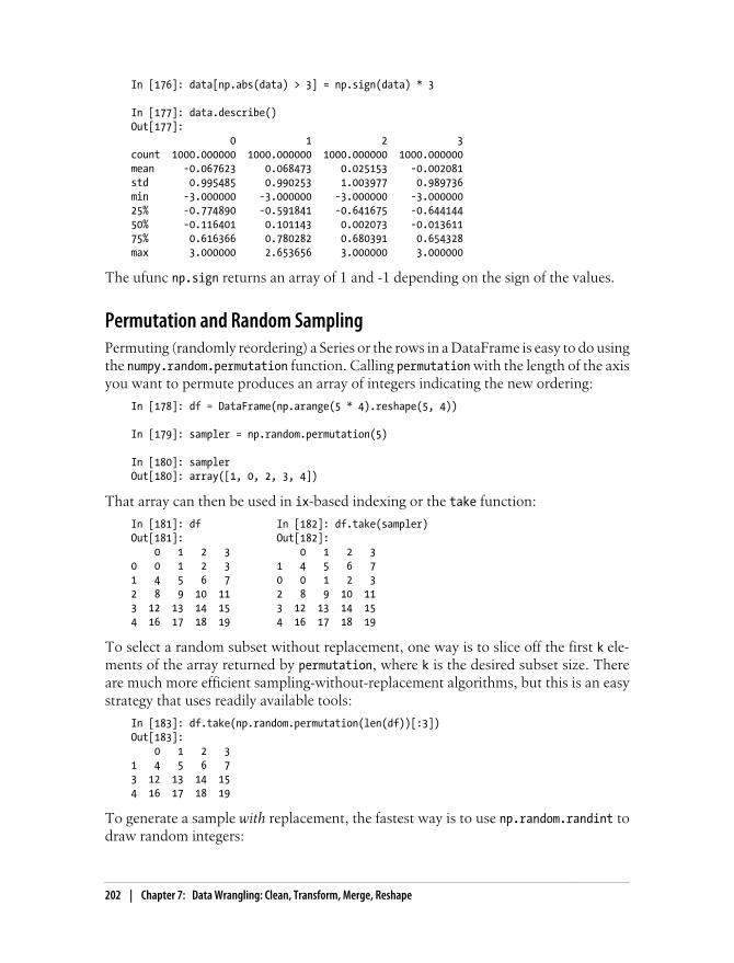
In [176]: data[np.abs(data) > 3] = np.sign(data) * 3
In [177]: data.describe()Out[177]: 0 1 2 3count 1000.000000 1000.000000 1000.000000 1000.000000mean -0.067623 0.068473 0.025153 -0.002081std 0.995485 0.990253 1.003977 0.989736min -3.000000 -3.000000 -3.000000 -3.00000025% -0.774890 -0.591841 -0.641675 -0.64414450% -0.116401 0.101143 0.002073 -0.01361175% 0.616366 0.780282 0.680391 0.654328max 3.000000 2.653656 3.000000 3.000000
The ufunc np.sign returns an array of 1 and -1 depending on the sign of the values.
Permutation and Random SamplingPermuting (randomly reordering) a Series or the rows in a DataFrame is easy to do usingthe numpy.random.permutation function. Calling permutation with the length of the axisyou want to permute produces an array of integers indicating the new ordering:
In [178]: df = DataFrame(np.arange(5 * 4).reshape(5, 4))
In [179]: sampler = np.random.permutation(5)
In [180]: samplerOut[180]: array([1, 0, 2, 3, 4])
That array can then be used in ix-based indexing or the take function:
In [181]: df In [182]: df.take(sampler)Out[181]: Out[182]: 0 1 2 3 0 1 2 30 0 1 2 3 1 4 5 6 71 4 5 6 7 0 0 1 2 32 8 9 10 11 2 8 9 10 113 12 13 14 15 3 12 13 14 154 16 17 18 19 4 16 17 18 19
To select a random subset without replacement, one way is to slice off the first k ele-ments of the array returned by permutation, where k is the desired subset size. Thereare much more efficient sampling-without-replacement algorithms, but this is an easystrategy that uses readily available tools:
In [183]: df.take(np.random.permutation(len(df))[:3])Out[183]: 0 1 2 31 4 5 6 73 12 13 14 154 16 17 18 19
To generate a sample with replacement, the fastest way is to use np.random.randint todraw random integers:
202 | Chapter 7: Data Wrangling: Clean, Transform, Merge, Reshape
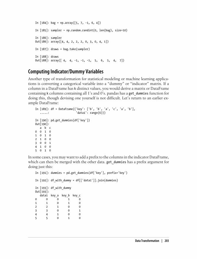
In [184]: bag = np.array([5, 7, -1, 6, 4])
In [185]: sampler = np.random.randint(0, len(bag), size=10)
In [186]: samplerOut[186]: array([4, 4, 2, 2, 2, 0, 3, 0, 4, 1])
In [187]: draws = bag.take(sampler)
In [188]: drawsOut[188]: array([ 4, 4, -1, -1, -1, 5, 6, 5, 4, 7])
Computing Indicator/Dummy VariablesAnother type of transformation for statistical modeling or machine learning applica-tions is converting a categorical variable into a “dummy” or “indicator” matrix. If acolumn in a DataFrame has k distinct values, you would derive a matrix or DataFramecontaining k columns containing all 1’s and 0’s. pandas has a get_dummies function fordoing this, though devising one yourself is not difficult. Let’s return to an earlier ex-ample DataFrame:
In [189]: df = DataFrame({'key': ['b', 'b', 'a', 'c', 'a', 'b'], .....: 'data1': range(6)})
In [190]: pd.get_dummies(df['key'])Out[190]: a b c0 0 1 01 0 1 02 1 0 03 0 0 14 1 0 05 0 1 0
In some cases, you may want to add a prefix to the columns in the indicator DataFrame,which can then be merged with the other data. get_dummies has a prefix argument fordoing just this:
In [191]: dummies = pd.get_dummies(df['key'], prefix='key')
In [192]: df_with_dummy = df[['data1']].join(dummies)
In [193]: df_with_dummyOut[193]: data1 key_a key_b key_c0 0 0 1 01 1 0 1 02 2 1 0 03 3 0 0 14 4 1 0 05 5 0 1 0
Data Transformation | 203

If a row in a DataFrame belongs to multiple categories, things are a bit more compli-cated. Let’s return to the MovieLens 1M dataset from earlier in the book:
In [194]: mnames = ['movie_id', 'title', 'genres']
In [195]: movies = pd.read_table('ch07/movies.dat', sep='::', header=None, .....: names=mnames)
In [196]: movies[:10]Out[196]: movie_id title genres0 1 Toy Story (1995) Animation|Children's|Comedy1 2 Jumanji (1995) Adventure|Children's|Fantasy2 3 Grumpier Old Men (1995) Comedy|Romance3 4 Waiting to Exhale (1995) Comedy|Drama4 5 Father of the Bride Part II (1995) Comedy5 6 Heat (1995) Action|Crime|Thriller6 7 Sabrina (1995) Comedy|Romance7 8 Tom and Huck (1995) Adventure|Children's8 9 Sudden Death (1995) Action9 10 GoldenEye (1995) Action|Adventure|Thriller
Adding indicator variables for each genre requires a little bit of wrangling. First, weextract the list of unique genres in the dataset (using a nice set.union trick):
In [197]: genre_iter = (set(x.split('|')) for x in movies.genres)
In [198]: genres = sorted(set.union(*genre_iter))
Now, one way to construct the indicator DataFrame is to start with a DataFrame of allzeros:
In [199]: dummies = DataFrame(np.zeros((len(movies), len(genres))), columns=genres)
Now, iterate through each movie and set entries in each row of dummies to 1:
In [200]: for i, gen in enumerate(movies.genres): .....: dummies.ix[i, gen.split('|')] = 1
Then, as above, you can combine this with movies:
In [201]: movies_windic = movies.join(dummies.add_prefix('Genre_'))
In [202]: movies_windic.ix[0]Out[202]:movie_id 1title Toy Story (1995)genres Animation|Children's|ComedyGenre_Action 0Genre_Adventure 0Genre_Animation 1Genre_Children's 1Genre_Comedy 1Genre_Crime 0Genre_Documentary 0Genre_Drama 0Genre_Fantasy 0
204 | Chapter 7: Data Wrangling: Clean, Transform, Merge, Reshape

Genre_Film-Noir 0Genre_Horror 0Genre_Musical 0Genre_Mystery 0Genre_Romance 0Genre_Sci-Fi 0Genre_Thriller 0Genre_War 0Genre_Western 0Name: 0
For much larger data, this method of constructing indicator variableswith multiple membership is not especially speedy. A lower-level func-tion leveraging the internals of the DataFrame could certainly be writ-ten.
A useful recipe for statistical applications is to combine get_dummies with a discretiza-tion function like cut:
In [204]: values = np.random.rand(10)
In [205]: valuesOut[205]:array([ 0.9296, 0.3164, 0.1839, 0.2046, 0.5677, 0.5955, 0.9645, 0.6532, 0.7489, 0.6536])
In [206]: bins = [0, 0.2, 0.4, 0.6, 0.8, 1]
In [207]: pd.get_dummies(pd.cut(values, bins))Out[207]: (0, 0.2] (0.2, 0.4] (0.4, 0.6] (0.6, 0.8] (0.8, 1]0 0 0 0 0 11 0 1 0 0 02 1 0 0 0 03 0 1 0 0 04 0 0 1 0 05 0 0 1 0 06 0 0 0 0 17 0 0 0 1 08 0 0 0 1 09 0 0 0 1 0
String ManipulationPython has long been a popular data munging language in part due to its ease-of-usefor string and text processing. Most text operations are made simple with the stringobject’s built-in methods. For more complex pattern matching and text manipulations,regular expressions may be needed. pandas adds to the mix by enabling you to applystring and regular expressions concisely on whole arrays of data, additionally handlingthe annoyance of missing data.
String Manipulation | 205
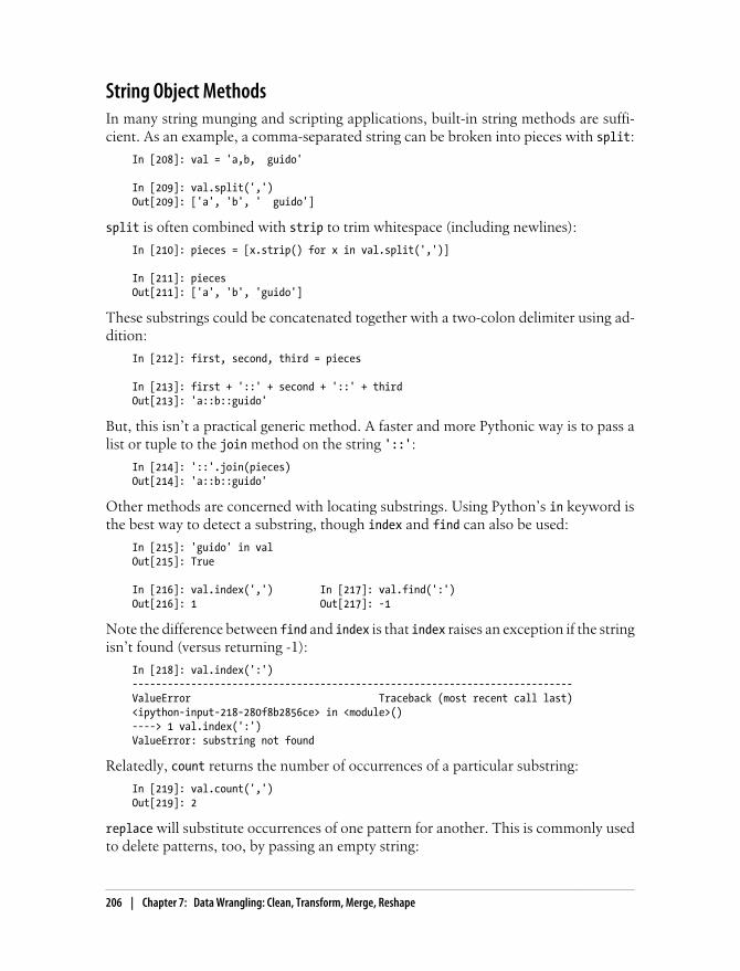
String Object MethodsIn many string munging and scripting applications, built-in string methods are suffi-cient. As an example, a comma-separated string can be broken into pieces with split:
In [208]: val = 'a,b, guido'
In [209]: val.split(',')Out[209]: ['a', 'b', ' guido']
split is often combined with strip to trim whitespace (including newlines):
In [210]: pieces = [x.strip() for x in val.split(',')]
In [211]: piecesOut[211]: ['a', 'b', 'guido']
These substrings could be concatenated together with a two-colon delimiter using ad-dition:
In [212]: first, second, third = pieces
In [213]: first + '::' + second + '::' + thirdOut[213]: 'a::b::guido'
But, this isn’t a practical generic method. A faster and more Pythonic way is to pass alist or tuple to the join method on the string '::':
In [214]: '::'.join(pieces)Out[214]: 'a::b::guido'
Other methods are concerned with locating substrings. Using Python’s in keyword isthe best way to detect a substring, though index and find can also be used:
In [215]: 'guido' in valOut[215]: True
In [216]: val.index(',') In [217]: val.find(':')Out[216]: 1 Out[217]: -1
Note the difference between find and index is that index raises an exception if the stringisn’t found (versus returning -1):
In [218]: val.index(':')---------------------------------------------------------------------------ValueError Traceback (most recent call last)<ipython-input-218-280f8b2856ce> in <module>()----> 1 val.index(':')ValueError: substring not found
Relatedly, count returns the number of occurrences of a particular substring:
In [219]: val.count(',')Out[219]: 2
replace will substitute occurrences of one pattern for another. This is commonly usedto delete patterns, too, by passing an empty string:
206 | Chapter 7: Data Wrangling: Clean, Transform, Merge, Reshape

In [220]: val.replace(',', '::') In [221]: val.replace(',', '')Out[220]: 'a::b:: guido' Out[221]: 'ab guido'
Regular expressions can also be used with many of these operations as you’ll see below.
Table 7-3. Python built-in string methods
Argument Description
count Return the number of non-overlapping occurrences of substring in the string.
endswith, startswith Returns True if string ends with suffix (starts with prefix).
join Use string as delimiter for concatenating a sequence of other strings.
index Return position of first character in substring if found in the string. Raises ValueError if not found.
find Return position of first character of first occurrence of substring in the string. Likeindex, but returns -1 if not found.
rfind Return position of first character of last occurrence of substring in the string. Returns -1if not found.
replace Replace occurrences of string with another string.
strip, rstrip, lstrip Trim whitespace, including newlines; equivalent to x.strip() (and rstrip,lstrip, respectively) for each element.
split Break string into list of substrings using passed delimiter.
lower, upper Convert alphabet characters to lowercase or uppercase, respectively.
ljust, rjust Left justify or right justify, respectively. Pad opposite side of string with spaces (or someother fill character) to return a string with a minimum width.
Regular expressionsRegular expressions provide a flexible way to search or match string patterns in text. Asingle expression, commonly called a regex, is a string formed according to the regularexpression language. Python’s built-in re module is responsible for applying regularexpressions to strings; I’ll give a number of examples of its use here.
The art of writing regular expressions could be a chapter of its own andthus is outside the book’s scope. There are many excellent tutorials andreferences on the internet, such as Zed Shaw’s Learn Regex The HardWay (http://regex.learncodethehardway.org/book/).
The re module functions fall into three categories: pattern matching, substitution, andsplitting. Naturally these are all related; a regex describes a pattern to locate in the text,which can then be used for many purposes. Let’s look at a simple example: suppose Iwanted to split a string with a variable number of whitespace characters (tabs, spaces,and newlines). The regex describing one or more whitespace characters is \s+:
String Manipulation | 207

In [222]: import re
In [223]: text = "foo bar\t baz \tqux"
In [224]: re.split('\s+', text)Out[224]: ['foo', 'bar', 'baz', 'qux']
When you call re.split('\s+', text), the regular expression is first compiled, then itssplit method is called on the passed text. You can compile the regex yourself with re.compile, forming a reusable regex object:
In [225]: regex = re.compile('\s+')
In [226]: regex.split(text)Out[226]: ['foo', 'bar', 'baz', 'qux']
If, instead, you wanted to get a list of all patterns matching the regex, you can use the findall method:
In [227]: regex.findall(text)Out[227]: [' ', '\t ', ' \t']
To avoid unwanted escaping with \ in a regular expression, use rawstring literals like r'C:\x' instead of the equivalent 'C:\\x'.
Creating a regex object with re.compile is highly recommended if you intend to applythe same expression to many strings; doing so will save CPU cycles.
match and search are closely related to findall. While findall returns all matches in astring, search returns only the first match. More rigidly, match only matches at thebeginning of the string. As a less trivial example, let’s consider a block of text and aregular expression capable of identifying most email addresses:
text = """Dave [email protected] [email protected] [email protected] [email protected]"""pattern = r'[A-Z0-9._%+-]+@[A-Z0-9.-]+\.[A-Z]{2,4}'
# re.IGNORECASE makes the regex case-insensitiveregex = re.compile(pattern, flags=re.IGNORECASE)
Using findall on the text produces a list of the e-mail addresses:
In [229]: regex.findall(text)Out[229]: ['[email protected]', '[email protected]', '[email protected]', '[email protected]']
search returns a special match object for the first email address in the text. For theabove regex, the match object can only tell us the start and end position of the patternin the string:
208 | Chapter 7: Data Wrangling: Clean, Transform, Merge, Reshape

In [230]: m = regex.search(text)
In [231]: mOut[231]: <_sre.SRE_Match at 0x10a05de00>
In [232]: text[m.start():m.end()]Out[232]: '[email protected]'
regex.match returns None, as it only will match if the pattern occurs at the start of thestring:
In [233]: print regex.match(text)None
Relatedly, sub will return a new string with occurrences of the pattern replaced by thea new string:
In [234]: print regex.sub('REDACTED', text)Dave REDACTEDSteve REDACTEDRob REDACTEDRyan REDACTED
Suppose you wanted to find email addresses and simultaneously segment each addressinto its 3 components: username, domain name, and domain suffix. To do this, putparentheses around the parts of the pattern to segment:
In [235]: pattern = r'([A-Z0-9._%+-]+)@([A-Z0-9.-]+)\.([A-Z]{2,4})'
In [236]: regex = re.compile(pattern, flags=re.IGNORECASE)
A match object produced by this modified regex returns a tuple of the pattern compo-nents with its groups method:
In [237]: m = regex.match('[email protected]')
In [238]: m.groups()Out[238]: ('wesm', 'bright', 'net')
findall returns a list of tuples when the pattern has groups:
In [239]: regex.findall(text)Out[239]:[('dave', 'google', 'com'), ('steve', 'gmail', 'com'), ('rob', 'gmail', 'com'), ('ryan', 'yahoo', 'com')]
sub also has access to groups in each match using special symbols like \1, \2, etc.:
In [240]: print regex.sub(r'Username: \1, Domain: \2, Suffix: \3', text)Dave Username: dave, Domain: google, Suffix: comSteve Username: steve, Domain: gmail, Suffix: comRob Username: rob, Domain: gmail, Suffix: comRyan Username: ryan, Domain: yahoo, Suffix: com
String Manipulation | 209
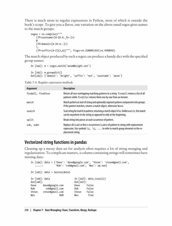
There is much more to regular expressions in Python, most of which is outside thebook’s scope. To give you a flavor, one variation on the above email regex gives namesto the match groups:
regex = re.compile(r""" (?P<username>[A-Z0-9._%+-]+) @ (?P<domain>[A-Z0-9.-]+) \. (?P<suffix>[A-Z]{2,4})""", flags=re.IGNORECASE|re.VERBOSE)
The match object produced by such a regex can produce a handy dict with the specifiedgroup names:
In [242]: m = regex.match('[email protected]')
In [243]: m.groupdict()Out[243]: {'domain': 'bright', 'suffix': 'net', 'username': 'wesm'}
Table 7-4. Regular expression methods
Argument Description
findall, finditer Return all non-overlapping matching patterns in a string. findall returns a list of allpatterns while finditer returns them one by one from an iterator.
match Match pattern at start of string and optionally segment pattern components into groups.If the pattern matches, returns a match object, otherwise None.
search Scan string for match to pattern; returning a match object if so. Unlike match, the matchcan be anywhere in the string as opposed to only at the beginning.
split Break string into pieces at each occurrence of pattern.
sub, subn Replace all (sub) or first n occurrences (subn) of pattern in string with replacementexpression. Use symbols \1, \2, ... to refer to match group elements in the re-placement string.
Vectorized string functions in pandasCleaning up a messy data set for analysis often requires a lot of string munging andregularization. To complicate matters, a column containing strings will sometimes havemissing data:
In [244]: data = {'Dave': '[email protected]', 'Steve': '[email protected]', .....: 'Rob': '[email protected]', 'Wes': np.nan}
In [245]: data = Series(data)
In [246]: data In [247]: data.isnull()Out[246]: Out[247]:Dave [email protected] Dave FalseRob [email protected] Rob FalseSteve [email protected] Steve FalseWes NaN Wes True
210 | Chapter 7: Data Wrangling: Clean, Transform, Merge, Reshape
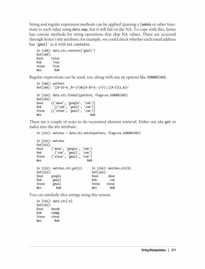
String and regular expression methods can be applied (passing a lambda or other func-tion) to each value using data.map, but it will fail on the NA. To cope with this, Serieshas concise methods for string operations that skip NA values. These are accessedthrough Series’s str attribute; for example, we could check whether each email addresshas 'gmail' in it with str.contains:
In [248]: data.str.contains('gmail')Out[248]:Dave FalseRob TrueSteve TrueWes NaN
Regular expressions can be used, too, along with any re options like IGNORECASE:
In [249]: patternOut[249]: '([A-Z0-9._%+-]+)@([A-Z0-9.-]+)\\.([A-Z]{2,4})'
In [250]: data.str.findall(pattern, flags=re.IGNORECASE)Out[250]:Dave [('dave', 'google', 'com')]Rob [('rob', 'gmail', 'com')]Steve [('steve', 'gmail', 'com')]Wes NaN
There are a couple of ways to do vectorized element retrieval. Either use str.get orindex into the str attribute:
In [251]: matches = data.str.match(pattern, flags=re.IGNORECASE)
In [252]: matchesOut[252]:Dave ('dave', 'google', 'com')Rob ('rob', 'gmail', 'com')Steve ('steve', 'gmail', 'com')Wes NaN
In [253]: matches.str.get(1) In [254]: matches.str[0]Out[253]: Out[254]:Dave google Dave daveRob gmail Rob robSteve gmail Steve steveWes NaN Wes NaN
You can similarly slice strings using this syntax:
In [255]: data.str[:5]Out[255]:Dave dave@Rob rob@gSteve steveWes NaN
String Manipulation | 211

Table 7-5. Vectorized string methods
Method Description
cat Concatenate strings element-wise with optional delimiter
contains Return boolean array if each string contains pattern/regex
count Count occurrences of pattern
endswith, startswith Equivalent to x.endswith(pattern) or x.startswith(pattern) for each el-ement.
findall Compute list of all occurrences of pattern/regex for each string
get Index into each element (retrieve i-th element)
join Join strings in each element of the Series with passed separator
len Compute length of each string
lower, upper Convert cases; equivalent to x.lower() or x.upper() for each element.
match Use re.match with the passed regular expression on each element, returning matchedgroups as list.
pad Add whitespace to left, right, or both sides of strings
center Equivalent to pad(side='both')
repeat Duplicate values; for example s.str.repeat(3) equivalent to x * 3 for each string.
replace Replace occurrences of pattern/regex with some other string
slice Slice each string in the Series.
split Split strings on delimiter or regular expression
strip, rstrip, lstrip Trim whitespace, including newlines; equivalent to x.strip() (and rstrip,lstrip, respectively) for each element.
Example: USDA Food DatabaseThe US Department of Agriculture makes available a database of food nutrient infor-mation. Ashley Williams, an English hacker, has made available a version of this da-tabase in JSON format (http://ashleyw.co.uk/project/food-nutrient-database). The re-cords look like this:
{ "id": 21441, "description": "KENTUCKY FRIED CHICKEN, Fried Chicken, EXTRA CRISPY,Wing, meat and skin with breading", "tags": ["KFC"], "manufacturer": "Kentucky Fried Chicken", "group": "Fast Foods", "portions": [ { "amount": 1, "unit": "wing, with skin", "grams": 68.0 },
212 | Chapter 7: Data Wrangling: Clean, Transform, Merge, Reshape

... ], "nutrients": [ { "value": 20.8, "units": "g", "description": "Protein", "group": "Composition" },
... ]}
Each food has a number of identifying attributes along with two lists of nutrients andportion sizes. Having the data in this form is not particularly amenable for analysis, sowe need to do some work to wrangle the data into a better form.
After downloading and extracting the data from the link above, you can load it intoPython with any JSON library of your choosing. I’ll use the built-in Python json mod-ule:
In [256]: import json
In [257]: db = json.load(open('ch07/foods-2011-10-03.json'))
In [258]: len(db)Out[258]: 6636
Each entry in db is a dict containing all the data for a single food. The 'nutrients' fieldis a list of dicts, one for each nutrient:
In [259]: db[0].keys() In [260]: db[0]['nutrients'][0]Out[259]: Out[260]:[u'portions', {u'description': u'Protein', u'description', u'group': u'Composition', u'tags', u'units': u'g', u'nutrients', u'value': 25.18} u'group', u'id', u'manufacturer']
In [261]: nutrients = DataFrame(db[0]['nutrients'])
In [262]: nutrients[:7]Out[262]: description group units value0 Protein Composition g 25.181 Total lipid (fat) Composition g 29.202 Carbohydrate, by difference Composition g 3.063 Ash Other g 3.284 Energy Energy kcal 376.005 Water Composition g 39.286 Energy Energy kJ 1573.00
Example: USDA Food Database | 213

When converting a list of dicts to a DataFrame, we can specify a list of fields to extract.We’ll take the food names, group, id, and manufacturer:
In [263]: info_keys = ['description', 'group', 'id', 'manufacturer']
In [264]: info = DataFrame(db, columns=info_keys)
In [265]: info[:5]Out[265]: description group id manufacturer0 Cheese, caraway Dairy and Egg Products 10081 Cheese, cheddar Dairy and Egg Products 10092 Cheese, edam Dairy and Egg Products 10183 Cheese, feta Dairy and Egg Products 10194 Cheese, mozzarella, part skim milk Dairy and Egg Products 1028
In [266]: infoOut[266]:<class 'pandas.core.frame.DataFrame'>Int64Index: 6636 entries, 0 to 6635Data columns:description 6636 non-null valuesgroup 6636 non-null valuesid 6636 non-null valuesmanufacturer 5195 non-null valuesdtypes: int64(1), object(3)
You can see the distribution of food groups with value_counts:
In [267]: pd.value_counts(info.group)[:10]Out[267]:Vegetables and Vegetable Products 812Beef Products 618Baked Products 496Breakfast Cereals 403Legumes and Legume Products 365Fast Foods 365Lamb, Veal, and Game Products 345Sweets 341Pork Products 328Fruits and Fruit Juices 328
Now, to do some analysis on all of the nutrient data, it’s easiest to assemble the nutrientsfor each food into a single large table. To do so, we need to take several steps. First, I’llconvert each list of food nutrients to a DataFrame, add a column for the food id, andappend the DataFrame to a list. Then, these can be concatenated together with concat:
nutrients = []
for rec in db: fnuts = DataFrame(rec['nutrients']) fnuts['id'] = rec['id'] nutrients.append(fnuts)
nutrients = pd.concat(nutrients, ignore_index=True)
214 | Chapter 7: Data Wrangling: Clean, Transform, Merge, Reshape
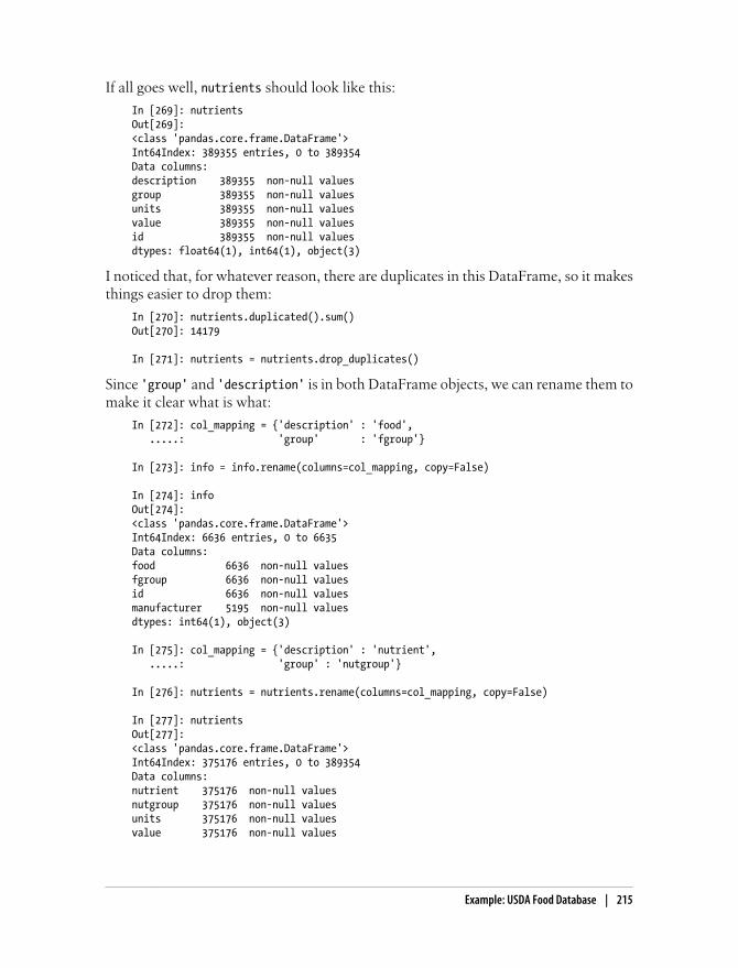
If all goes well, nutrients should look like this:
In [269]: nutrientsOut[269]:<class 'pandas.core.frame.DataFrame'>Int64Index: 389355 entries, 0 to 389354Data columns:description 389355 non-null valuesgroup 389355 non-null valuesunits 389355 non-null valuesvalue 389355 non-null valuesid 389355 non-null valuesdtypes: float64(1), int64(1), object(3)
I noticed that, for whatever reason, there are duplicates in this DataFrame, so it makesthings easier to drop them:
In [270]: nutrients.duplicated().sum()Out[270]: 14179
In [271]: nutrients = nutrients.drop_duplicates()
Since 'group' and 'description' is in both DataFrame objects, we can rename them tomake it clear what is what:
In [272]: col_mapping = {'description' : 'food', .....: 'group' : 'fgroup'}
In [273]: info = info.rename(columns=col_mapping, copy=False)
In [274]: infoOut[274]:<class 'pandas.core.frame.DataFrame'>Int64Index: 6636 entries, 0 to 6635Data columns:food 6636 non-null valuesfgroup 6636 non-null valuesid 6636 non-null valuesmanufacturer 5195 non-null valuesdtypes: int64(1), object(3)
In [275]: col_mapping = {'description' : 'nutrient', .....: 'group' : 'nutgroup'}
In [276]: nutrients = nutrients.rename(columns=col_mapping, copy=False)
In [277]: nutrientsOut[277]:<class 'pandas.core.frame.DataFrame'>Int64Index: 375176 entries, 0 to 389354Data columns:nutrient 375176 non-null valuesnutgroup 375176 non-null valuesunits 375176 non-null valuesvalue 375176 non-null values
Example: USDA Food Database | 215
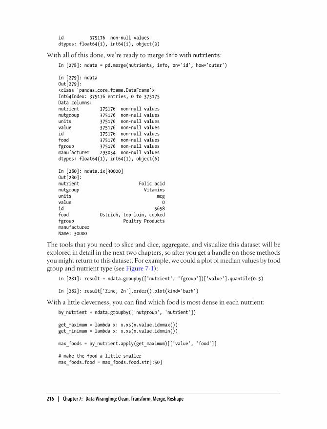
id 375176 non-null valuesdtypes: float64(1), int64(1), object(3)
With all of this done, we’re ready to merge info with nutrients:
In [278]: ndata = pd.merge(nutrients, info, on='id', how='outer')
In [279]: ndataOut[279]:<class 'pandas.core.frame.DataFrame'>Int64Index: 375176 entries, 0 to 375175Data columns:nutrient 375176 non-null valuesnutgroup 375176 non-null valuesunits 375176 non-null valuesvalue 375176 non-null valuesid 375176 non-null valuesfood 375176 non-null valuesfgroup 375176 non-null valuesmanufacturer 293054 non-null valuesdtypes: float64(1), int64(1), object(6)
In [280]: ndata.ix[30000]Out[280]:nutrient Folic acidnutgroup Vitaminsunits mcgvalue 0id 5658food Ostrich, top loin, cookedfgroup Poultry ProductsmanufacturerName: 30000
The tools that you need to slice and dice, aggregate, and visualize this dataset will beexplored in detail in the next two chapters, so after you get a handle on those methodsyou might return to this dataset. For example, we could a plot of median values by foodgroup and nutrient type (see Figure 7-1):
In [281]: result = ndata.groupby(['nutrient', 'fgroup'])['value'].quantile(0.5)
In [282]: result['Zinc, Zn'].order().plot(kind='barh')
With a little cleverness, you can find which food is most dense in each nutrient:
by_nutrient = ndata.groupby(['nutgroup', 'nutrient'])
get_maximum = lambda x: x.xs(x.value.idxmax())get_minimum = lambda x: x.xs(x.value.idxmin())
max_foods = by_nutrient.apply(get_maximum)[['value', 'food']]
# make the food a little smallermax_foods.food = max_foods.food.str[:50]
216 | Chapter 7: Data Wrangling: Clean, Transform, Merge, Reshape
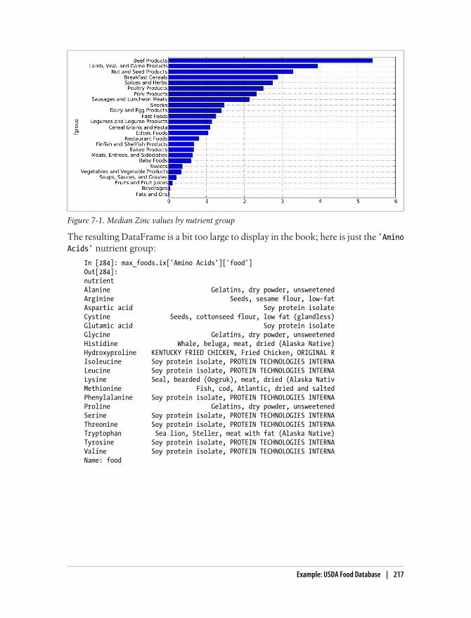
The resulting DataFrame is a bit too large to display in the book; here is just the 'AminoAcids' nutrient group:
In [284]: max_foods.ix['Amino Acids']['food']Out[284]:nutrientAlanine Gelatins, dry powder, unsweetenedArginine Seeds, sesame flour, low-fatAspartic acid Soy protein isolateCystine Seeds, cottonseed flour, low fat (glandless)Glutamic acid Soy protein isolateGlycine Gelatins, dry powder, unsweetenedHistidine Whale, beluga, meat, dried (Alaska Native)Hydroxyproline KENTUCKY FRIED CHICKEN, Fried Chicken, ORIGINAL RIsoleucine Soy protein isolate, PROTEIN TECHNOLOGIES INTERNALeucine Soy protein isolate, PROTEIN TECHNOLOGIES INTERNALysine Seal, bearded (Oogruk), meat, dried (Alaska NativMethionine Fish, cod, Atlantic, dried and saltedPhenylalanine Soy protein isolate, PROTEIN TECHNOLOGIES INTERNAProline Gelatins, dry powder, unsweetenedSerine Soy protein isolate, PROTEIN TECHNOLOGIES INTERNAThreonine Soy protein isolate, PROTEIN TECHNOLOGIES INTERNATryptophan Sea lion, Steller, meat with fat (Alaska Native)Tyrosine Soy protein isolate, PROTEIN TECHNOLOGIES INTERNAValine Soy protein isolate, PROTEIN TECHNOLOGIES INTERNAName: food
Figure 7-1. Median Zinc values by nutrient group
Example: USDA Food Database | 217

CHAPTER 8
Plotting and Visualization
Making plots and static or interactive visualizations is one of the most important tasksin data analysis. It may be a part of the exploratory process; for example, helping iden-tify outliers, needed data transformations, or coming up with ideas for models. Forothers, building an interactive visualization for the web using a toolkit like d3.js (http://d3js.org/) may be the end goal. Python has many visualization tools (see the end ofthis chapter), but I’ll be mainly focused on matplotlib (http://matplotlib.sourceforge.net).
matplotlib is a (primarily 2D) desktop plotting package designed for creating publica-tion-quality plots. The project was started by John Hunter in 2002 to enable a MAT-LAB-like plotting interface in Python. He, Fernando Pérez (of IPython), and others havecollaborated for many years since then to make IPython combined with matplotlib avery functional and productive environment for scientific computing. When used intandem with a GUI toolkit (for example, within IPython), matplotlib has interactivefeatures like zooming and panning. It supports many different GUI backends on alloperating systems and additionally can export graphics to all of the common vectorand raster graphics formats: PDF, SVG, JPG, PNG, BMP, GIF, etc. I have used it toproduce almost all of the graphics outside of diagrams in this book.
matplotlib has a number of add-on toolkits, such as mplot3d for 3D plots and basemapfor mapping and projections. I will give an example using basemap to plot data on a mapand to read shapefiles at the end of the chapter.
To follow along with the code examples in the chapter, make sure you have startedIPython in Pylab mode (ipython --pylab) or enabled GUI event loop integration withthe %gui magic.
A Brief matplotlib API PrimerThere are several ways to interact with matplotlib. The most common is through pylabmode in IPython by running ipython --pylab. This launches IPython configured to beable to support the matplotlib GUI backend of your choice (Tk, wxPython, PyQt, Mac
219

OS X native, GTK). For most users, the default backend will be sufficient. Pylab modealso imports a large set of modules and functions into IPython to provide a more MAT-LAB-like interface. You can test that everything is working by making a simple plot:
plot(np.arange(10))
If everything is set up right, a new window should pop up with a line plot. You canclose it by using the mouse or entering close(). Matplotlib API functions like plot and close are all in the matplotlib.pyplot module, which is typically imported by conven-tion as:
import matplotlib.pyplot as plt
While the pandas plotting functions described later deal with many of the mundanedetails of making plots, should you wish to customize them beyond the function op-tions provided you will need to learn a bit about the matplotlib API.
There is not enough room in the book to give a comprehensive treatmentto the breadth and depth of functionality in matplotlib. It should beenough to teach you the ropes to get up and running. The matplotlibgallery and documentation are the best resource for becoming a plottingguru and using advanced features.
Figures and SubplotsPlots in matplotlib reside within a Figure object. You can create a new figure withplt.figure:
In [13]: fig = plt.figure()
Figure 8-1. A more complex matplotlib financial plot
220 | Chapter 8: Plotting and Visualization
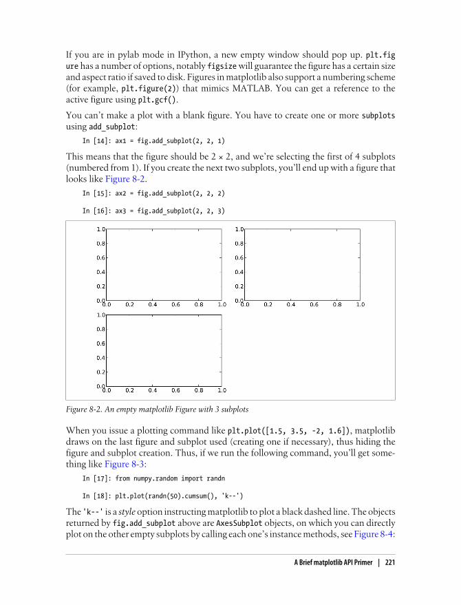
If you are in pylab mode in IPython, a new empty window should pop up. plt.figure has a number of options, notably figsize will guarantee the figure has a certain sizeand aspect ratio if saved to disk. Figures in matplotlib also support a numbering scheme(for example, plt.figure(2)) that mimics MATLAB. You can get a reference to theactive figure using plt.gcf().
You can’t make a plot with a blank figure. You have to create one or more subplotsusing add_subplot:
In [14]: ax1 = fig.add_subplot(2, 2, 1)
This means that the figure should be 2 × 2, and we’re selecting the first of 4 subplots(numbered from 1). If you create the next two subplots, you’ll end up with a figure thatlooks like Figure 8-2.
In [15]: ax2 = fig.add_subplot(2, 2, 2)
In [16]: ax3 = fig.add_subplot(2, 2, 3)
Figure 8-2. An empty matplotlib Figure with 3 subplots
When you issue a plotting command like plt.plot([1.5, 3.5, -2, 1.6]), matplotlibdraws on the last figure and subplot used (creating one if necessary), thus hiding thefigure and subplot creation. Thus, if we run the following command, you’ll get some-thing like Figure 8-3:
In [17]: from numpy.random import randn
In [18]: plt.plot(randn(50).cumsum(), 'k--')
The 'k--' is a style option instructing matplotlib to plot a black dashed line. The objectsreturned by fig.add_subplot above are AxesSubplot objects, on which you can directlyplot on the other empty subplots by calling each one’s instance methods, see Figure 8-4:
A Brief matplotlib API Primer | 221

In [19]: _ = ax1.hist(randn(100), bins=20, color='k', alpha=0.3)
In [20]: ax2.scatter(np.arange(30), np.arange(30) + 3 * randn(30))
You can find a comprehensive catalogue of plot types in the matplotlib documentation.
Since creating a figure with multiple subplots according to a particular layout is sucha common task, there is a convenience method, plt.subplots, that creates a new figureand returns a NumPy array containing the created subplot objects:
Figure 8-3. Figure after single plot
Figure 8-4. Figure after additional plots
222 | Chapter 8: Plotting and Visualization
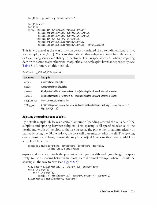
In [22]: fig, axes = plt.subplots(2, 3)
In [23]: axesOut[23]: array([[Axes(0.125,0.536364;0.227941x0.363636), Axes(0.398529,0.536364;0.227941x0.363636), Axes(0.672059,0.536364;0.227941x0.363636)], [Axes(0.125,0.1;0.227941x0.363636), Axes(0.398529,0.1;0.227941x0.363636), Axes(0.672059,0.1;0.227941x0.363636)]], dtype=object)
This is very useful as the axes array can be easily indexed like a two-dimensional array;for example, axes[0, 1]. You can also indicate that subplots should have the same Xor Y axis using sharex and sharey, respectively. This is especially useful when comparingdata on the same scale; otherwise, matplotlib auto-scales plot limits independently. SeeTable 8-1 for more on this method.
Table 8-1. pyplot.subplots options
Argument Description
nrows Number of rows of subplots
ncols Number of columns of subplots
sharex All subplots should use the same X-axis ticks (adjusting the xlim will affect all subplots)
sharey All subplots should use the same Y-axis ticks (adjusting the ylim will affect all subplots)
subplot_kw Dict of keywords for creating the
**fig_kw Additional keywords to subplots are used when creating the figure, such as plt.subplots(2, 2,figsize=(8, 6))
Adjusting the spacing around subplots
By default matplotlib leaves a certain amount of padding around the outside of thesubplots and spacing between subplots. This spacing is all specified relative to theheight and width of the plot, so that if you resize the plot either programmatically ormanually using the GUI window, the plot will dynamically adjust itself. The spacingcan be most easily changed using the subplots_adjust Figure method, also available asa top-level function:
subplots_adjust(left=None, bottom=None, right=None, top=None, wspace=None, hspace=None)
wspace and hspace controls the percent of the figure width and figure height, respec-tively, to use as spacing between subplots. Here is a small example where I shrink thespacing all the way to zero (see Figure 8-5):
fig, axes = plt.subplots(2, 2, sharex=True, sharey=True)for i in range(2): for j in range(2): axes[i, j].hist(randn(500), bins=50, color='k', alpha=0.5)plt.subplots_adjust(wspace=0, hspace=0)
A Brief matplotlib API Primer | 223

Figure 8-5. Figure with no inter-subplot spacing
You may notice that the axis labels overlap. matplotlib doesn’t check whether the labelsoverlap, so in a case like this you would need to fix the labels yourself by specifyingexplicit tick locations and tick labels. More on this in the coming sections.
Colors, Markers, and Line StylesMatplotlib’s main plot function accepts arrays of X and Y coordinates and optionallya string abbreviation indicating color and line style. For example, to plot x versus y withgreen dashes, you would execute:
ax.plot(x, y, 'g--')
This way of specifying both color and linestyle in a string is provided as a convenience;in practice if you were creating plots programmatically you might prefer not to have tomunge strings together to create plots with the desired style. The same plot could alsohave been expressed more explicitly as:
ax.plot(x, y, linestyle='--', color='g')
There are a number of color abbreviations provided for commonly-used colors, but anycolor on the spectrum can be used by specifying its RGB value (for example, '#CECECE'). You can see the full set of linestyles by looking at the docstring for plot.
Line plots can additionally have markers to highlight the actual data points. Since mat-plotlib creates a continuous line plot, interpolating between points, it can occasionallybe unclear where the points lie. The marker can be part of the style string, which musthave color followed by marker type and line style (see Figure 8-6):
In [28]: plt.plot(randn(30).cumsum(), 'ko--')
224 | Chapter 8: Plotting and Visualization

This could also have been written more explicitly as:
plot(randn(30).cumsum(), color='k', linestyle='dashed', marker='o')
For line plots, you will notice that subsequent points are linearly interpolated by de-fault. This can be altered with the drawstyle option:
In [30]: data = randn(30).cumsum()
In [31]: plt.plot(data, 'k--', label='Default')Out[31]: [<matplotlib.lines.Line2D at 0x461cdd0>]
In [32]: plt.plot(data, 'k-', drawstyle='steps-post', label='steps-post')Out[32]: [<matplotlib.lines.Line2D at 0x461f350>]
In [33]: plt.legend(loc='best')
Ticks, Labels, and LegendsFor most kinds of plot decorations, there are two main ways to do things: using theprocedural pyplot interface (which will be very familiar to MATLAB users) and themore object-oriented native matplotlib API.
The pyplot interface, designed for interactive use, consists of methods like xlim,xticks, and xticklabels. These control the plot range, tick locations, and tick labels,respectively. They can be used in two ways:
• Called with no arguments returns the current parameter value. For example plt.xlim() returns the current X axis plotting range
Figure 8-6. Line plot with markers example
A Brief matplotlib API Primer | 225
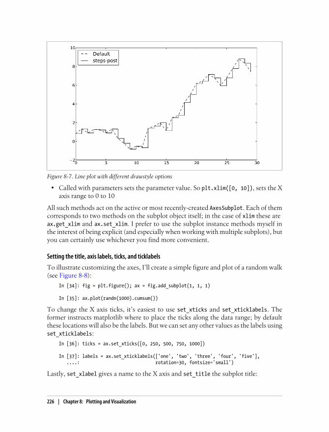
• Called with parameters sets the parameter value. So plt.xlim([0, 10]), sets the Xaxis range to 0 to 10
All such methods act on the active or most recently-created AxesSubplot. Each of themcorresponds to two methods on the subplot object itself; in the case of xlim these are ax.get_xlim and ax.set_xlim. I prefer to use the subplot instance methods myself inthe interest of being explicit (and especially when working with multiple subplots), butyou can certainly use whichever you find more convenient.
Setting the title, axis labels, ticks, and ticklabels
To illustrate customizing the axes, I’ll create a simple figure and plot of a random walk(see Figure 8-8):
In [34]: fig = plt.figure(); ax = fig.add_subplot(1, 1, 1)
In [35]: ax.plot(randn(1000).cumsum())
To change the X axis ticks, it’s easiest to use set_xticks and set_xticklabels. Theformer instructs matplotlib where to place the ticks along the data range; by defaultthese locations will also be the labels. But we can set any other values as the labels usingset_xticklabels:
In [36]: ticks = ax.set_xticks([0, 250, 500, 750, 1000])
In [37]: labels = ax.set_xticklabels(['one', 'two', 'three', 'four', 'five'], ....: rotation=30, fontsize='small')
Lastly, set_xlabel gives a name to the X axis and set_title the subplot title:
Figure 8-7. Line plot with different drawstyle options
226 | Chapter 8: Plotting and Visualization
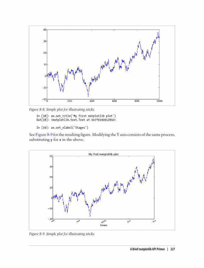
In [38]: ax.set_title('My first matplotlib plot')Out[38]: <matplotlib.text.Text at 0x7f9190912850>
In [39]: ax.set_xlabel('Stages')
See Figure 8-9 for the resulting figure. Modifying the Y axis consists of the same process,substituting y for x in the above.
Figure 8-9. Simple plot for illustrating xticks
Figure 8-8. Simple plot for illustrating xticks
A Brief matplotlib API Primer | 227
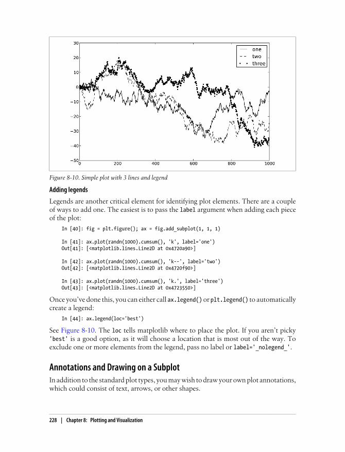
Adding legends
Legends are another critical element for identifying plot elements. There are a coupleof ways to add one. The easiest is to pass the label argument when adding each pieceof the plot:
In [40]: fig = plt.figure(); ax = fig.add_subplot(1, 1, 1)
In [41]: ax.plot(randn(1000).cumsum(), 'k', label='one')Out[41]: [<matplotlib.lines.Line2D at 0x4720a90>]
In [42]: ax.plot(randn(1000).cumsum(), 'k--', label='two')Out[42]: [<matplotlib.lines.Line2D at 0x4720f90>]
In [43]: ax.plot(randn(1000).cumsum(), 'k.', label='three')Out[43]: [<matplotlib.lines.Line2D at 0x4723550>]
Once you’ve done this, you can either call ax.legend() or plt.legend() to automaticallycreate a legend:
In [44]: ax.legend(loc='best')
See Figure 8-10. The loc tells matplotlib where to place the plot. If you aren’t picky'best' is a good option, as it will choose a location that is most out of the way. Toexclude one or more elements from the legend, pass no label or label='_nolegend_'.
Annotations and Drawing on a SubplotIn addition to the standard plot types, you may wish to draw your own plot annotations,which could consist of text, arrows, or other shapes.
Figure 8-10. Simple plot with 3 lines and legend
228 | Chapter 8: Plotting and Visualization

Annotations and text can be added using the text, arrow, and annotate functions.text draws text at given coordinates (x, y) on the plot with optional custom styling:
ax.text(x, y, 'Hello world!', family='monospace', fontsize=10)
Annotations can draw both text and arrows arranged appropriately. As an example,let’s plot the closing S&P 500 index price since 2007 (obtained from Yahoo! Finance)and annotate it with some of the important dates from the 2008-2009 financial crisis.See Figure 8-11 for the result:
from datetime import datetime
fig = plt.figure()ax = fig.add_subplot(1, 1, 1)
data = pd.read_csv('ch08/spx.csv', index_col=0, parse_dates=True)spx = data['SPX']
spx.plot(ax=ax, style='k-')
crisis_data = [ (datetime(2007, 10, 11), 'Peak of bull market'), (datetime(2008, 3, 12), 'Bear Stearns Fails'), (datetime(2008, 9, 15), 'Lehman Bankruptcy')]
for date, label in crisis_data: ax.annotate(label, xy=(date, spx.asof(date) + 50), xytext=(date, spx.asof(date) + 200), arrowprops=dict(facecolor='black'), horizontalalignment='left', verticalalignment='top')
# Zoom in on 2007-2010ax.set_xlim(['1/1/2007', '1/1/2011'])ax.set_ylim([600, 1800])
ax.set_title('Important dates in 2008-2009 financial crisis')
See the online matplotlib gallery for many more annotation examples to learn from.
Drawing shapes requires some more care. matplotlib has objects that represent manycommon shapes, referred to as patches. Some of these, like Rectangle and Circle arefound in matplotlib.pyplot, but the full set is located in matplotlib.patches.
To add a shape to a plot, you create the patch object shp and add it to a subplot bycalling ax.add_patch(shp) (see Figure 8-12):
fig = plt.figure()ax = fig.add_subplot(1, 1, 1)
rect = plt.Rectangle((0.2, 0.75), 0.4, 0.15, color='k', alpha=0.3)circ = plt.Circle((0.7, 0.2), 0.15, color='b', alpha=0.3)pgon = plt.Polygon([[0.15, 0.15], [0.35, 0.4], [0.2, 0.6]], color='g', alpha=0.5)
A Brief matplotlib API Primer | 229

ax.add_patch(rect)ax.add_patch(circ)ax.add_patch(pgon)
Figure 8-11. Important dates in 2008-2009 financial crisis
Figure 8-12. Figure composed from 3 different patches
If you look at the implementation of many familiar plot types, you will see that theyare assembled from patches.
230 | Chapter 8: Plotting and Visualization

Saving Plots to FileThe active figure can be saved to file using plt.savefig. This method is equivalent tothe figure object’s savefig instance method. For example, to save an SVG version of afigure, you need only type:
plt.savefig('figpath.svg')
The file type is inferred from the file extension. So if you used .pdf instead you wouldget a PDF. There are a couple of important options that I use frequently for publishinggraphics: dpi, which controls the dots-per-inch resolution, and bbox_inches, which cantrim the whitespace around the actual figure. To get the same plot as a PNG above withminimal whitespace around the plot and at 400 DPI, you would do:
plt.savefig('figpath.png', dpi=400, bbox_inches='tight')
savefig doesn’t have to write to disk; it can also write to any file-like object, such as aStringIO:
from io import StringIObuffer = StringIO()plt.savefig(buffer)plot_data = buffer.getvalue()
For example, this is useful for serving dynamically-generated images over the web.
Table 8-2. Figure.savefig options
Argument Description
fname String containing a filepath or a Python file-like object. The figure format is inferred from the fileextension, e.g. .pdf for PDF or .png for PNG.
dpi The figure resolution in dots per inch; defaults to 100 out of the box but can be configured
facecolor, edgecolor
The color of the figure background outside of the subplots. 'w' (white), by default
format The explicit file format to use ('png', 'pdf', 'svg', 'ps', 'eps', ...)
bbox_inches The portion of the figure to save. If 'tight' is passed, will attempt to trim the empty space aroundthe figure
matplotlib Configurationmatplotlib comes configured with color schemes and defaults that are geared primarilytoward preparing figures for publication. Fortunately, nearly all of the default behaviorcan be customized via an extensive set of global parameters governing figure size, sub-plot spacing, colors, font sizes, grid styles, and so on. There are two main ways tointeract with the matplotlib configuration system. The first is programmatically fromPython using the rc method. For example, to set the global default figure size to be 10x 10, you could enter:
plt.rc('figure', figsize=(10, 10))
A Brief matplotlib API Primer | 231

The first argument to rc is the component you wish to customize, such as 'figure','axes', 'xtick', 'ytick', 'grid', 'legend' or many others. After that can follow asequence of keyword arguments indicating the new parameters. An easy way to writedown the options in your program is as a dict:
font_options = {'family' : 'monospace', 'weight' : 'bold', 'size' : 'small'}plt.rc('font', **font_options)
For more extensive customization and to see a list of all the options, matplotlib comeswith a configuration file matplotlibrc in the matplotlib/mpl-data directory. If you cus-tomize this file and place it in your home directory titled .matplotlibrc, it will be loadedeach time you use matplotlib.
Plotting Functions in pandasAs you’ve seen, matplotlib is actually a fairly low-level tool. You assemble a plot fromits base components: the data display (the type of plot: line, bar, box, scatter, contour,etc.), legend, title, tick labels, and other annotations. Part of the reason for this is thatin many cases the data needed to make a complete plot is spread across many objects.In pandas we have row labels, column labels, and possibly grouping information. Thismeans that many kinds of fully-formed plots that would ordinarily require a lot ofmatplotlib code can be expressed in one or two concise statements. Therefore, pandashas an increasing number of high-level plotting methods for creating standard visual-izations that take advantage of how data is organized in DataFrame objects.
As of this writing, the plotting functionality in pandas is undergoingquite a bit of work. As part of the 2012 Google Summer of Code pro-gram, a student is working full time to add features and to make theinterface more consistent and usable. Thus, it’s possible that this codemay fall out-of-date faster than the other things in this book. The onlinepandas documentation will be the best resource in that event.
Line PlotsSeries and DataFrame each have a plot method for making many different plot types.By default, they make line plots (see Figure 8-13):
In [55]: s = Series(np.random.randn(10).cumsum(), index=np.arange(0, 100, 10))
In [56]: s.plot()
The Series object’s index is passed to matplotlib for plotting on the X axis, though thiscan be disabled by passing use_index=False. The X axis ticks and limits can be adjustedusing the xticks and xlim options, and Y axis respectively using yticks and ylim. See
232 | Chapter 8: Plotting and Visualization

Table 8-3 for a full listing of plot options. I’ll comment on a few more of them through-out this section and leave the rest to you to explore.
Most of pandas’s plotting methods accept an optional ax parameter, which can be amatplotlib subplot object. This gives you more flexible placement of subplots in a gridlayout. There will be more on this in the later section on the matplotlib API.
DataFrame’s plot method plots each of its columns as a different line on the samesubplot, creating a legend automatically (see Figure 8-14):
In [57]: df = DataFrame(np.random.randn(10, 4).cumsum(0), ....: columns=['A', 'B', 'C', 'D'], ....: index=np.arange(0, 100, 10))
In [58]: df.plot()
Additional keyword arguments to plot are passed through to the re-spective matplotlib plotting function, so you can further customizethese plots by learning more about the matplotlib API.
Table 8-3. Series.plot method arguments
Argument Description
label Label for plot legend
ax matplotlib subplot object to plot on. If nothing passed, uses active matplotlib subplot
style Style string, like 'ko--', to be passed to matplotlib.
alpha The plot fill opacity (from 0 to 1)
Figure 8-13. Simple Series plot example
Plotting Functions in pandas | 233
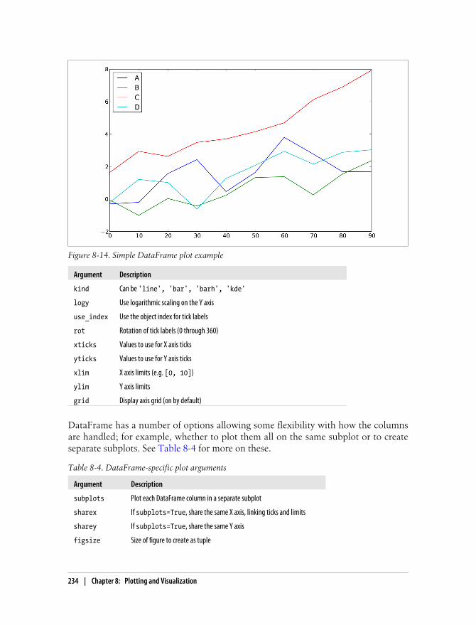
Argument Description
kind Can be 'line', 'bar', 'barh', 'kde'
logy Use logarithmic scaling on the Y axis
use_index Use the object index for tick labels
rot Rotation of tick labels (0 through 360)
xticks Values to use for X axis ticks
yticks Values to use for Y axis ticks
xlim X axis limits (e.g. [0, 10])
ylim Y axis limits
grid Display axis grid (on by default)
DataFrame has a number of options allowing some flexibility with how the columnsare handled; for example, whether to plot them all on the same subplot or to createseparate subplots. See Table 8-4 for more on these.
Table 8-4. DataFrame-specific plot arguments
Argument Description
subplots Plot each DataFrame column in a separate subplot
sharex If subplots=True, share the same X axis, linking ticks and limits
sharey If subplots=True, share the same Y axis
figsize Size of figure to create as tuple
Figure 8-14. Simple DataFrame plot example
234 | Chapter 8: Plotting and Visualization
Argument Description
title Plot title as string
legend Add a subplot legend (True by default)
sort_columns Plot columns in alphabetical order; by default uses existing column order
For time series plotting, see Chapter 10.
Bar PlotsMaking bar plots instead of line plots is a simple as passing kind='bar' (for verticalbars) or kind='barh' (for horizontal bars). In this case, the Series or DataFrame indexwill be used as the X (bar) or Y (barh) ticks (see Figure 8-15):
In [59]: fig, axes = plt.subplots(2, 1)
In [60]: data = Series(np.random.rand(16), index=list('abcdefghijklmnop'))
In [61]: data.plot(kind='bar', ax=axes[0], color='k', alpha=0.7)Out[61]: <matplotlib.axes.AxesSubplot at 0x4ee7750>
In [62]: data.plot(kind='barh', ax=axes[1], color='k', alpha=0.7)
For more on the plt.subplots function and matplotlib axes and figures,see the later section in this chapter.
With a DataFrame, bar plots group the values in each row together in a group in bars,side by side, for each value. See Figure 8-16:
In [63]: df = DataFrame(np.random.rand(6, 4), ....: index=['one', 'two', 'three', 'four', 'five', 'six'], ....: columns=pd.Index(['A', 'B', 'C', 'D'], name='Genus'))
In [64]: dfOut[64]: Genus A B C Done 0.301686 0.156333 0.371943 0.270731two 0.750589 0.525587 0.689429 0.358974three 0.381504 0.667707 0.473772 0.632528four 0.942408 0.180186 0.708284 0.641783five 0.840278 0.909589 0.010041 0.653207six 0.062854 0.589813 0.811318 0.060217
In [65]: df.plot(kind='bar')
Plotting Functions in pandas | 235

Figure 8-15. Horizonal and vertical bar plot example
Note that the name “Genus” on the DataFrame’s columns is used to title the legend.
Stacked bar plots are created from a DataFrame by passing stacked=True, resulting inthe value in each row being stacked together (see Figure 8-17):
In [67]: df.plot(kind='barh', stacked=True, alpha=0.5)
A useful recipe for bar plots (as seen in an earlier chapter) is to visualizea Series’s value frequency using value_counts: s.value_counts().plot(kind='bar')
Returning to the tipping data set used earlier in the book, suppose we wanted to makea stacked bar plot showing the percentage of data points for each party size on eachday. I load the data using read_csv and make a cross-tabulation by day and party size:
In [68]: tips = pd.read_csv('ch08/tips.csv')
In [69]: party_counts = pd.crosstab(tips.day, tips.size)
In [70]: party_countsOut[70]: size 1 2 3 4 5 6day Fri 1 16 1 1 0 0Sat 2 53 18 13 1 0Sun 0 39 15 18 3 1Thur 1 48 4 5 1 3
236 | Chapter 8: Plotting and Visualization

# Not many 1- and 6-person partiesIn [71]: party_counts = party_counts.ix[:, 2:5]
Figure 8-16. DataFrame bar plot example
Figure 8-17. DataFrame stacked bar plot example
Then, normalize so that each row sums to 1 (I have to cast to float to avoid integerdivision issues on Python 2.7) and make the plot (see Figure 8-18):
# Normalize to sum to 1In [72]: party_pcts = party_counts.div(party_counts.sum(1).astype(float), axis=0)
Plotting Functions in pandas | 237

In [73]: party_pctsOut[73]: size 2 3 4 5day Fri 0.888889 0.055556 0.055556 0.000000Sat 0.623529 0.211765 0.152941 0.011765Sun 0.520000 0.200000 0.240000 0.040000Thur 0.827586 0.068966 0.086207 0.017241
In [74]: party_pcts.plot(kind='bar', stacked=True)
Figure 8-18. Fraction of parties by size on each day
So you can see that party sizes appear to increase on the weekend in this data set.
Histograms and Density PlotsA histogram, with which you may be well-acquainted, is a kind of bar plot that gives adiscretized display of value frequency. The data points are split into discrete, evenlyspaced bins, and the number of data points in each bin is plotted. Using the tippingdata from before, we can make a histogram of tip percentages of the total bill using the hist method on the Series (see Figure 8-19):
In [76]: tips['tip_pct'] = tips['tip'] / tips['total_bill']
In [77]: tips['tip_pct'].hist(bins=50)
238 | Chapter 8: Plotting and Visualization

Figure 8-19. Histogram of tip percentages
A related plot type is a density plot, which is formed by computing an estimate of acontinuous probability distribution that might have generated the observed data. Ausual procedure is to approximate this distribution as a mixture of kernels, that is,simpler distributions like the normal (Gaussian) distribution. Thus, density plots arealso known as KDE (kernel density estimate) plots. Using plot with kind='kde' makesa density plot using the standard mixture-of-normals KDE (see Figure 8-20):
In [79]: tips['tip_pct'].plot(kind='kde')
These two plot types are often plotted together; the histogram in normalized form (togive a binned density) with a kernel density estimate plotted on top. As an example,consider a bimodal distribution consisting of draws from two different standard normaldistributions (see Figure 8-21):
In [81]: comp1 = np.random.normal(0, 1, size=200) # N(0, 1)
In [82]: comp2 = np.random.normal(10, 2, size=200) # N(10, 4)
In [83]: values = Series(np.concatenate([comp1, comp2]))
In [84]: values.hist(bins=100, alpha=0.3, color='k', normed=True)Out[84]: <matplotlib.axes.AxesSubplot at 0x5cd2350>
In [85]: values.plot(kind='kde', style='k--')
Scatter PlotsScatter plots are a useful way of examining the relationship between two one-dimen-sional data series. matplotlib has a scatter plotting method that is the workhorse of
Plotting Functions in pandas | 239

making these kinds of plots. To give an example, I load the macrodata dataset from thestatsmodels project, select a few variables, then compute log differences:
In [86]: macro = pd.read_csv('ch08/macrodata.csv')
In [87]: data = macro[['cpi', 'm1', 'tbilrate', 'unemp']]
In [88]: trans_data = np.log(data).diff().dropna()
Figure 8-20. Density plot of tip percentages
Figure 8-21. Normalized histogram of normal mixture with density estimate
240 | Chapter 8: Plotting and Visualization
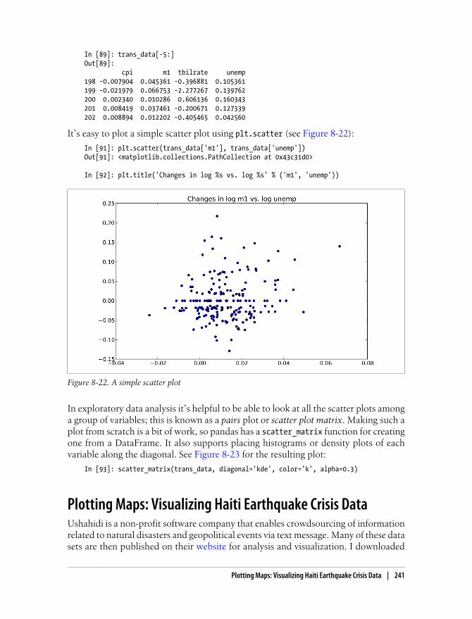
In [89]: trans_data[-5:]Out[89]: cpi m1 tbilrate unemp198 -0.007904 0.045361 -0.396881 0.105361199 -0.021979 0.066753 -2.277267 0.139762200 0.002340 0.010286 0.606136 0.160343201 0.008419 0.037461 -0.200671 0.127339202 0.008894 0.012202 -0.405465 0.042560
It’s easy to plot a simple scatter plot using plt.scatter (see Figure 8-22):
In [91]: plt.scatter(trans_data['m1'], trans_data['unemp'])Out[91]: <matplotlib.collections.PathCollection at 0x43c31d0>
In [92]: plt.title('Changes in log %s vs. log %s' % ('m1', 'unemp'))
Figure 8-22. A simple scatter plot
In exploratory data analysis it’s helpful to be able to look at all the scatter plots amonga group of variables; this is known as a pairs plot or scatter plot matrix. Making such aplot from scratch is a bit of work, so pandas has a scatter_matrix function for creatingone from a DataFrame. It also supports placing histograms or density plots of eachvariable along the diagonal. See Figure 8-23 for the resulting plot:
In [93]: scatter_matrix(trans_data, diagonal='kde', color='k', alpha=0.3)
Plotting Maps: Visualizing Haiti Earthquake Crisis DataUshahidi is a non-profit software company that enables crowdsourcing of informationrelated to natural disasters and geopolitical events via text message. Many of these datasets are then published on their website for analysis and visualization. I downloaded
Plotting Maps: Visualizing Haiti Earthquake Crisis Data | 241
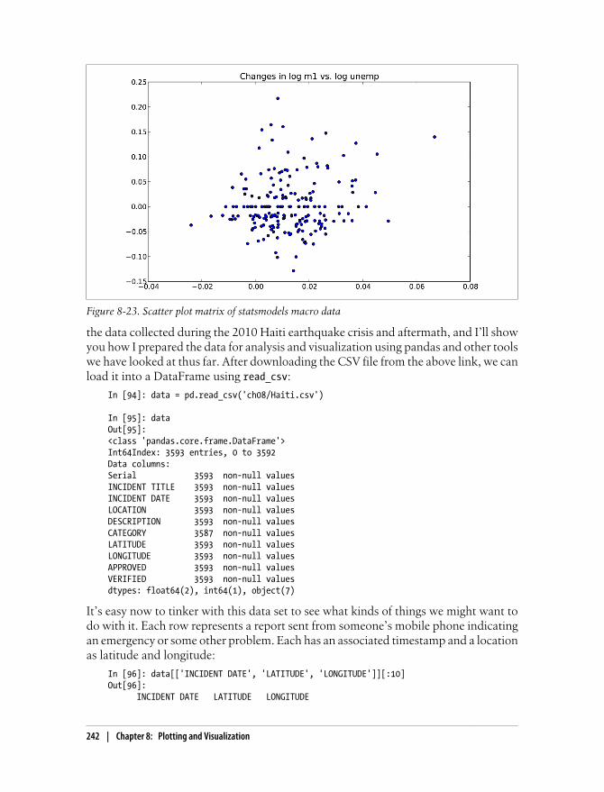
the data collected during the 2010 Haiti earthquake crisis and aftermath, and I’ll showyou how I prepared the data for analysis and visualization using pandas and other toolswe have looked at thus far. After downloading the CSV file from the above link, we canload it into a DataFrame using read_csv:
In [94]: data = pd.read_csv('ch08/Haiti.csv')
In [95]: dataOut[95]: <class 'pandas.core.frame.DataFrame'>Int64Index: 3593 entries, 0 to 3592Data columns:Serial 3593 non-null valuesINCIDENT TITLE 3593 non-null valuesINCIDENT DATE 3593 non-null valuesLOCATION 3593 non-null valuesDESCRIPTION 3593 non-null valuesCATEGORY 3587 non-null valuesLATITUDE 3593 non-null valuesLONGITUDE 3593 non-null valuesAPPROVED 3593 non-null valuesVERIFIED 3593 non-null valuesdtypes: float64(2), int64(1), object(7)
It’s easy now to tinker with this data set to see what kinds of things we might want todo with it. Each row represents a report sent from someone’s mobile phone indicatingan emergency or some other problem. Each has an associated timestamp and a locationas latitude and longitude:
In [96]: data[['INCIDENT DATE', 'LATITUDE', 'LONGITUDE']][:10]Out[96]: INCIDENT DATE LATITUDE LONGITUDE
Figure 8-23. Scatter plot matrix of statsmodels macro data
242 | Chapter 8: Plotting and Visualization

0 05/07/2010 17:26 18.233333 -72.5333331 28/06/2010 23:06 50.226029 5.7298862 24/06/2010 16:21 22.278381 114.1742873 20/06/2010 21:59 44.407062 8.9339894 18/05/2010 16:26 18.571084 -72.3346715 26/04/2010 13:14 18.593707 -72.3100796 26/04/2010 14:19 18.482800 -73.6388007 26/04/2010 14:27 18.415000 -73.1950008 15/03/2010 10:58 18.517443 -72.2368419 15/03/2010 11:00 18.547790 -72.410010
The CATEGORY field contains a comma-separated list of codes indicating the type ofmessage:
In [97]: data['CATEGORY'][:6]Out[97]: 0 1. Urgences | Emergency, 3. Public Health, 1 1. Urgences | Emergency, 2. Urgences logistiques 2 2. Urgences logistiques | Vital Lines, 8. Autre |3 1. Urgences | Emergency, 4 1. Urgences | Emergency, 5 5e. Communication lines down, Name: CATEGORY
If you notice above in the data summary, some of the categories are missing, so wemight want to drop these data points. Additionally, calling describe shows that thereare some aberrant locations:
In [98]: data.describe()Out[98]: Serial LATITUDE LONGITUDEcount 3593.000000 3593.000000 3593.000000mean 2080.277484 18.611495 -72.322680std 1171.100360 0.738572 3.650776min 4.000000 18.041313 -74.45275725% 1074.000000 18.524070 -72.41750050% 2163.000000 18.539269 -72.33500075% 3088.000000 18.561820 -72.293570max 4052.000000 50.226029 114.174287
Cleaning the bad locations and removing the missing categories is now fairly simple:
In [99]: data = data[(data.LATITUDE > 18) & (data.LATITUDE < 20) & ....: (data.LONGITUDE > -75) & (data.LONGITUDE < -70) ....: & data.CATEGORY.notnull()]
Now we might want to do some analysis or visualization of this data by category, buteach category field may have multiple categories. Additionally, each category is givenas a code plus an English and possibly also a French code name. Thus, a little bit ofwrangling is required to get the data into a more agreeable form. First, I wrote thesetwo functions to get a list of all the categories and to split each category into a code andan English name:
def to_cat_list(catstr): stripped = (x.strip() for x in catstr.split(','))
Plotting Maps: Visualizing Haiti Earthquake Crisis Data | 243

return [x for x in stripped if x]
def get_all_categories(cat_series): cat_sets = (set(to_cat_list(x)) for x in cat_series) return sorted(set.union(*cat_sets))
def get_english(cat): code, names = cat.split('.') if '|' in names: names = names.split(' | ')[1] return code, names.strip()
You can test out that the get_english function does what you expect:
In [101]: get_english('2. Urgences logistiques | Vital Lines')Out[101]: ('2', 'Vital Lines')
Now, I make a dict mapping code to name because we’ll use the codes for analysis.We’ll use this later when adorning plots (note the use of a generator expression in lieuof a list comprehension):
In [102]: all_cats = get_all_categories(data.CATEGORY)
# Generator expressionIn [103]: english_mapping = dict(get_english(x) for x in all_cats)
In [104]: english_mapping['2a']Out[104]: 'Food Shortage'
In [105]: english_mapping['6c']Out[105]: 'Earthquake and aftershocks'
There are many ways to go about augmenting the data set to be able to easily selectrecords by category. One way is to add indicator (or dummy) columns, one for eachcategory. To do that, first extract the unique category codes and construct a DataFrameof zeros having those as its columns and the same index as data:
def get_code(seq): return [x.split('.')[0] for x in seq if x]
all_codes = get_code(all_cats)code_index = pd.Index(np.unique(all_codes))dummy_frame = DataFrame(np.zeros((len(data), len(code_index))), index=data.index, columns=code_index)
If all goes well, dummy_frame should look something like this:
In [107]: dummy_frame.ix[:, :6]Out[107]: <class 'pandas.core.frame.DataFrame'>Int64Index: 3569 entries, 0 to 3592Data columns:1 3569 non-null values1a 3569 non-null values1b 3569 non-null values1c 3569 non-null values
244 | Chapter 8: Plotting and Visualization

1d 3569 non-null values2 3569 non-null valuesdtypes: float64(6)
As you recall, the trick is then to set the appropriate entries of each row to 1, lastlyjoining this with data:
for row, cat in zip(data.index, data.CATEGORY): codes = get_code(to_cat_list(cat)) dummy_frame.ix[row, codes] = 1
data = data.join(dummy_frame.add_prefix('category_'))
data finally now has new columns like:
In [109]: data.ix[:, 10:15]Out[109]: <class 'pandas.core.frame.DataFrame'>Int64Index: 3569 entries, 0 to 3592Data columns:category_1 3569 non-null valuescategory_1a 3569 non-null valuescategory_1b 3569 non-null valuescategory_1c 3569 non-null valuescategory_1d 3569 non-null valuesdtypes: float64(5)
Let’s make some plots! As this is spatial data, we’d like to plot the data by category ona map of Haiti. The basemap toolkit (http://matplotlib.github.com/basemap), an add-onto matplotlib, enables plotting 2D data on maps in Python. basemap provides manydifferent globe projections and a means for transforming projecting latitude and lon-gitude coordinates on the globe onto a two-dimensional matplotlib plot. After sometrial and error and using the above data as a guideline, I wrote this function which drawsa simple black and white map of Haiti:
from mpl_toolkits.basemap import Basemapimport matplotlib.pyplot as plt
def basic_haiti_map(ax=None, lllat=17.25, urlat=20.25, lllon=-75, urlon=-71): # create polar stereographic Basemap instance. m = Basemap(ax=ax, projection='stere', lon_0=(urlon + lllon) / 2, lat_0=(urlat + lllat) / 2, llcrnrlat=lllat, urcrnrlat=urlat, llcrnrlon=lllon, urcrnrlon=urlon, resolution='f') # draw coastlines, state and country boundaries, edge of map. m.drawcoastlines() m.drawstates() m.drawcountries() return m
The idea, now, is that the returned Basemap object, knows how to transform coordinatesonto the canvas. I wrote the following code to plot the data observations for a number
Plotting Maps: Visualizing Haiti Earthquake Crisis Data | 245

of report categories. For each category, I filter down the data set to the coordinateslabeled by that category, plot a Basemap on the appropriate subplot, transform the co-ordinates, then plot the points using the Basemap’s plot method:
fig, axes = plt.subplots(nrows=2, ncols=2, figsize=(12, 10))fig.subplots_adjust(hspace=0.05, wspace=0.05)
to_plot = ['2a', '1', '3c', '7a']
lllat=17.25; urlat=20.25; lllon=-75; urlon=-71
for code, ax in zip(to_plot, axes.flat): m = basic_haiti_map(ax, lllat=lllat, urlat=urlat, lllon=lllon, urlon=urlon)
cat_data = data[data['category_%s' % code] == 1]
# compute map proj coordinates. x, y = m(cat_data.LONGITUDE, cat_data.LATITUDE)
m.plot(x, y, 'k.', alpha=0.5) ax.set_title('%s: %s' % (code, english_mapping[code]))
The resulting figure can be seen in Figure 8-24.
It seems from the plot that most of the data is concentrated around the most populouscity, Port-au-Prince. basemap allows you to overlap additional map data which comesfrom what are called shapefiles. I first downloaded a shapefile with roads in Port-au-Prince (see http://cegrp.cga.harvard.edu/haiti/?q=resources_data). The Basemap objectconveniently has a readshapefile method so that, after extracting the road data archive,I added just the following lines to my code:
Figure 8-24. Haiti crisis data for 4 categories
246 | Chapter 8: Plotting and Visualization

shapefile_path = 'ch08/PortAuPrince_Roads/PortAuPrince_Roads'm.readshapefile(shapefile_path, 'roads')
After a little more trial and error with the latitude and longitude boundaries, I was ableto make Figure 8-25 for the “Food shortage” category.
Python Visualization Tool EcosystemAs is common with open source, there are a plethora of options for creating graphicsin Python (too many to list). In addition to open source, there are numerous commerciallibraries with Python bindings.
In this chapter and throughout the book, I have been primarily concerned with mat-plotlib as it is the most widely used plotting tool in Python. While it’s an importantpart of the scientific Python ecosystem, matplotlib has plenty of shortcomings when itcomes to the creation and display of statistical graphics. MATLAB users will likely findmatplotlib familiar, while R users (especially users of the excellent ggplot2 and trellis packages) may be somewhat disappointed (at least as of this writing). It is possibleto make beautiful plots for display on the web in matplotlib, but doing so often requiressignificant effort as the library is designed for the printed page. Aesthetics aside, it issufficient for most needs. In pandas, I, along with the other developers, have sought tobuild a convenient user interface that makes it easier to make most kinds of plots com-monplace in data analysis.
There are a number of other visualization tools in wide use. I list a few of them hereand encourage you to explore the ecosystem.
Figure 8-25. Food shortage reports in Port-au-Prince during the Haiti earthquake crisis
Python Visualization Tool Ecosystem | 247

ChacoChaco (http://code.enthought.com/chaco/), developed by Enthought, is a plotting tool-kit suitable both for static plotting and interactive visualizations. It is especially well-suited for expressing complex visualizations with data interrelationships. Comparedwith matplotlib, Chaco has much better support for interacting with plot elements andrendering is very fast, making it a good choice for building interactive GUI applications.
Figure 8-26. A Chaco example plot
mayaviThe mayavi project, developed by Prabhu Ramachandran, Gaël Varoquaux, and others,is a 3D graphics toolkit built on the open source C++ graphics library VTK. mayavi,like matplotlib, integrates with IPython so that it is easy to use interactively. The plotscan be panned, rotated, and zoomed using the mouse and keyboard. I used mayavi tomake one of the illustrations of broadcasting in Chapter 12. While I don’t show anymayavi-using code here, there is plenty of documentation and examples available on-line. In many cases, I believe it is a good alternative to a technology like WebGL, thoughthe graphics are harder to share in interactive form.
Other PackagesOf course, there are numerous other visualization libraries and applications availablein Python: PyQwt, Veusz, gnuplot-py, biggles, and others. I have seen PyQwt put togood use in GUI applications built using the Qt application framework using PyQt.While many of these libraries continue to be under active development (some of them
248 | Chapter 8: Plotting and Visualization

are part of much larger applications), I have noted in the last few years a general trendtoward web-based technologies and away from desktop graphics. I’ll say a few morewords about this in the next section.
The Future of Visualization Tools?Visualizations built on web technologies (that is, JavaScript-based) appear to be theinevitable future. Doubtlessly you have used many different kinds of static or interactivevisualizations built in Flash or JavaScript over the years. New toolkits (such as d3.jsand its numerous off-shoot projects) for building such displays are appearing all thetime. In contrast, development in non web-based visualization has slowed significantlyin recent years. This holds true of Python as well as other data analysis and statisticalcomputing environments like R.
The development challenge, then, will be in building tighter integration between dataanalysis and preparation tools, such as pandas, and the web browser. I am hopeful thatthis will become a fruitful point of collaboration between Python and non-Python usersas well.
Python Visualization Tool Ecosystem | 249

CHAPTER 9
Data Aggregation and GroupOperations
Categorizing a data set and applying a function to each group, whether an aggregationor transformation, is often a critical component of a data analysis workflow. Afterloading, merging, and preparing a data set, a familiar task is to compute group statisticsor possibly pivot tables for reporting or visualization purposes. pandas provides a flex-ible and high-performance groupby facility, enabling you to slice and dice, and sum-marize data sets in a natural way.
One reason for the popularity of relational databases and SQL (which stands for“structured query language”) is the ease with which data can be joined, filtered, trans-formed, and aggregated. However, query languages like SQL are rather limited in thekinds of group operations that can be performed. As you will see, with the expressive-ness and power of Python and pandas, we can perform much more complex groupedoperations by utilizing any function that accepts a pandas object or NumPy array. Inthis chapter, you will learn how to:
• Split a pandas object into pieces using one or more keys (in the form of functions,arrays, or DataFrame column names)
• Computing group summary statistics, like count, mean, or standard deviation, ora user-defined function
• Apply a varying set of functions to each column of a DataFrame
• Apply within-group transformations or other manipulations, like normalization,linear regression, rank, or subset selection
• Compute pivot tables and cross-tabulations
• Perform quantile analysis and other data-derived group analyses
251

Aggregation of time series data, a special use case of groupby, is referredto as resampling in this book and will receive separate treatment inChapter 10.
GroupBy MechanicsHadley Wickham, an author of many popular packages for the R programming lan-guage, coined the term split-apply-combine for talking about group operations, and Ithink that’s a good description of the process. In the first stage of the process, datacontained in a pandas object, whether a Series, DataFrame, or otherwise, is split intogroups based on one or more keys that you provide. The splitting is performed on aparticular axis of an object. For example, a DataFrame can be grouped on its rows(axis=0) or its columns (axis=1). Once this is done, a function is applied to each group,producing a new value. Finally, the results of all those function applications are com-bined into a result object. The form of the resulting object will usually depend on what’sbeing done to the data. See Figure 9-1 for a mockup of a simple group aggregation.
Figure 9-1. Illustration of a group aggregation
Each grouping key can take many forms, and the keys do not have to be all of the sametype:
• A list or array of values that is the same length as the axis being grouped
• A value indicating a column name in a DataFrame
252 | Chapter 9: Data Aggregation and Group Operations

• A dict or Series giving a correspondence between the values on the axis beinggrouped and the group names
• A function to be invoked on the axis index or the individual labels in the index
Note that the latter three methods are all just shortcuts for producing an array of valuesto be used to split up the object. Don’t worry if this all seems very abstract. Throughoutthis chapter, I will give many examples of all of these methods. To get started, here isa very simple small tabular dataset as a DataFrame:
In [13]: df = DataFrame({'key1' : ['a', 'a', 'b', 'b', 'a'], ....: 'key2' : ['one', 'two', 'one', 'two', 'one'], ....: 'data1' : np.random.randn(5), ....: 'data2' : np.random.randn(5)})
In [14]: dfOut[14]: data1 data2 key1 key20 -0.204708 1.393406 a one1 0.478943 0.092908 a two2 -0.519439 0.281746 b one3 -0.555730 0.769023 b two4 1.965781 1.246435 a one
Suppose you wanted to compute the mean of the data1 column using the groups labelsfrom key1. There are a number of ways to do this. One is to access data1 and callgroupby with the column (a Series) at key1:
In [15]: grouped = df['data1'].groupby(df['key1'])
In [16]: groupedOut[16]: <pandas.core.groupby.SeriesGroupBy at 0x2d78b10>
This grouped variable is now a GroupBy object. It has not actually computed anythingyet except for some intermediate data about the group key df['key1']. The idea is thatthis object has all of the information needed to then apply some operation to each ofthe groups. For example, to compute group means we can call the GroupBy’s meanmethod:
In [17]: grouped.mean()Out[17]: key1a 0.746672b -0.537585
Later, I'll explain more about what’s going on when you call .mean(). The importantthing here is that the data (a Series) has been aggregated according to the group key,producing a new Series that is now indexed by the unique values in the key1 column.The result index has the name 'key1' because the DataFrame column df['key1'] did.
If instead we had passed multiple arrays as a list, we get something different:
In [18]: means = df['data1'].groupby([df['key1'], df['key2']]).mean()
GroupBy Mechanics | 253

In [19]: meansOut[19]: key1 key2a one 0.880536 two 0.478943b one -0.519439 two -0.555730
In this case, we grouped the data using two keys, and the resulting Series now has ahierarchical index consisting of the unique pairs of keys observed:
In [20]: means.unstack()Out[20]: key2 one twokey1 a 0.880536 0.478943b -0.519439 -0.555730
In these examples, the group keys are all Series, though they could be any arrays of theright length:
In [21]: states = np.array(['Ohio', 'California', 'California', 'Ohio', 'Ohio'])
In [22]: years = np.array([2005, 2005, 2006, 2005, 2006])
In [23]: df['data1'].groupby([states, years]).mean()Out[23]: California 2005 0.478943 2006 -0.519439Ohio 2005 -0.380219 2006 1.965781
Frequently the grouping information to be found in the same DataFrame as the datayou want to work on. In that case, you can pass column names (whether those arestrings, numbers, or other Python objects) as the group keys:
In [24]: df.groupby('key1').mean()Out[24]: data1 data2key1 a 0.746672 0.910916b -0.537585 0.525384
In [25]: df.groupby(['key1', 'key2']).mean()Out[25]: data1 data2key1 key2 a one 0.880536 1.319920 two 0.478943 0.092908b one -0.519439 0.281746 two -0.555730 0.769023
You may have noticed in the first case df.groupby('key1').mean() that there is nokey2 column in the result. Because df['key2'] is not numeric data, it is said to be anuisance column, which is therefore excluded from the result. By default, all of the
254 | Chapter 9: Data Aggregation and Group Operations

numeric columns are aggregated, though it is possible to filter down to a subset as you’llsee soon.
Regardless of the objective in using groupby, a generally useful GroupBy method is size which return a Series containing group sizes:
In [26]: df.groupby(['key1', 'key2']).size()Out[26]: key1 key2a one 2 two 1b one 1 two 1
As of this writing, any missing values in a group key will be excludedfrom the result. It’s possible (and, in fact, quite likely), that by the timeyou are reading this there will be an option to include the NA group inthe result.
Iterating Over GroupsThe GroupBy object supports iteration, generating a sequence of 2-tuples containingthe group name along with the chunk of data. Consider the following small exampledata set:
In [27]: for name, group in df.groupby('key1'): ....: print name ....: print group ....:a data1 data2 key1 key20 -0.204708 1.393406 a one1 0.478943 0.092908 a two4 1.965781 1.246435 a oneb data1 data2 key1 key22 -0.519439 0.281746 b one3 -0.555730 0.769023 b two
In the case of multiple keys, the first element in the tuple will be a tuple of key values:
In [28]: for (k1, k2), group in df.groupby(['key1', 'key2']): ....: print k1, k2 ....: print group ....:a one data1 data2 key1 key20 -0.204708 1.393406 a one4 1.965781 1.246435 a onea two data1 data2 key1 key21 0.478943 0.092908 a twob one data1 data2 key1 key2
GroupBy Mechanics | 255
2 -0.519439 0.281746 b oneb two data1 data2 key1 key23 -0.55573 0.769023 b two
Of course, you can choose to do whatever you want with the pieces of data. A recipeyou may find useful is computing a dict of the data pieces as a one-liner:
In [29]: pieces = dict(list(df.groupby('key1')))
In [30]: pieces['b']Out[30]: data1 data2 key1 key22 -0.519439 0.281746 b one3 -0.555730 0.769023 b two
By default groupby groups on axis=0, but you can group on any of the other axes. Forexample, we could group the columns of our example df here by dtype like so:
In [31]: df.dtypesOut[31]: data1 float64data2 float64key1 objectkey2 object
In [32]: grouped = df.groupby(df.dtypes, axis=1)
In [33]: dict(list(grouped))Out[33]: {dtype('float64'): data1 data20 -0.204708 1.3934061 0.478943 0.0929082 -0.519439 0.2817463 -0.555730 0.7690234 1.965781 1.246435, dtype('object'): key1 key20 a one1 a two2 b one3 b two4 a one}
Selecting a Column or Subset of ColumnsIndexing a GroupBy object created from a DataFrame with a column name or array ofcolumn names has the effect of selecting those columns for aggregation. This means that:
df.groupby('key1')['data1']df.groupby('key1')[['data2']]
are syntactic sugar for:
df['data1'].groupby(df['key1'])df[['data2']].groupby(df['key1'])
256 | Chapter 9: Data Aggregation and Group Operations
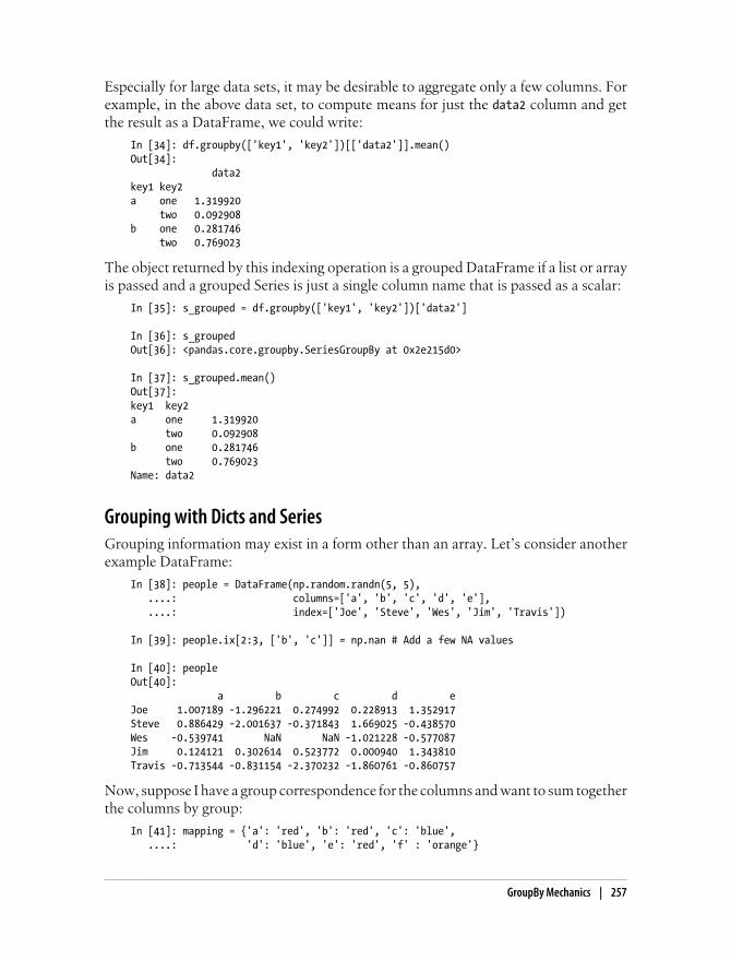
Especially for large data sets, it may be desirable to aggregate only a few columns. Forexample, in the above data set, to compute means for just the data2 column and getthe result as a DataFrame, we could write:
In [34]: df.groupby(['key1', 'key2'])[['data2']].mean()Out[34]: data2key1 key2 a one 1.319920 two 0.092908b one 0.281746 two 0.769023
The object returned by this indexing operation is a grouped DataFrame if a list or arrayis passed and a grouped Series is just a single column name that is passed as a scalar:
In [35]: s_grouped = df.groupby(['key1', 'key2'])['data2']
In [36]: s_groupedOut[36]: <pandas.core.groupby.SeriesGroupBy at 0x2e215d0>
In [37]: s_grouped.mean()Out[37]: key1 key2a one 1.319920 two 0.092908b one 0.281746 two 0.769023Name: data2
Grouping with Dicts and SeriesGrouping information may exist in a form other than an array. Let’s consider anotherexample DataFrame:
In [38]: people = DataFrame(np.random.randn(5, 5), ....: columns=['a', 'b', 'c', 'd', 'e'], ....: index=['Joe', 'Steve', 'Wes', 'Jim', 'Travis'])
In [39]: people.ix[2:3, ['b', 'c']] = np.nan # Add a few NA values
In [40]: peopleOut[40]: a b c d eJoe 1.007189 -1.296221 0.274992 0.228913 1.352917Steve 0.886429 -2.001637 -0.371843 1.669025 -0.438570Wes -0.539741 NaN NaN -1.021228 -0.577087Jim 0.124121 0.302614 0.523772 0.000940 1.343810Travis -0.713544 -0.831154 -2.370232 -1.860761 -0.860757
Now, suppose I have a group correspondence for the columns and want to sum togetherthe columns by group:
In [41]: mapping = {'a': 'red', 'b': 'red', 'c': 'blue', ....: 'd': 'blue', 'e': 'red', 'f' : 'orange'}
GroupBy Mechanics | 257

Now, you could easily construct an array from this dict to pass to groupby, but insteadwe can just pass the dict:
In [42]: by_column = people.groupby(mapping, axis=1)
In [43]: by_column.sum()Out[43]: blue redJoe 0.503905 1.063885Steve 1.297183 -1.553778Wes -1.021228 -1.116829Jim 0.524712 1.770545Travis -4.230992 -2.405455
The same functionality holds for Series, which can be viewed as a fixed size mapping.When I used Series as group keys in the above examples, pandas does, in fact, inspecteach Series to ensure that its index is aligned with the axis it’s grouping:
In [44]: map_series = Series(mapping)
In [45]: map_seriesOut[45]: a redb redc blued bluee redf orange
In [46]: people.groupby(map_series, axis=1).count()Out[46]: blue redJoe 2 3Steve 2 3Wes 1 2Jim 2 3Travis 2 3
Grouping with FunctionsUsing Python functions in what can be fairly creative ways is a more abstract way ofdefining a group mapping compared with a dict or Series. Any function passed as agroup key will be called once per index value, with the return values being used as thegroup names. More concretely, consider the example DataFrame from the previoussection, which has people’s first names as index values. Suppose you wanted to groupby the length of the names; you could compute an array of string lengths, but insteadyou can just pass the len function:
In [47]: people.groupby(len).sum()Out[47]: a b c d e3 0.591569 -0.993608 0.798764 -0.791374 2.119639
258 | Chapter 9: Data Aggregation and Group Operations

5 0.886429 -2.001637 -0.371843 1.669025 -0.4385706 -0.713544 -0.831154 -2.370232 -1.860761 -0.860757
Mixing functions with arrays, dicts, or Series is not a problem as everything gets con-verted to arrays internally:
In [48]: key_list = ['one', 'one', 'one', 'two', 'two']
In [49]: people.groupby([len, key_list]).min()Out[49]: a b c d e3 one -0.539741 -1.296221 0.274992 -1.021228 -0.577087 two 0.124121 0.302614 0.523772 0.000940 1.3438105 one 0.886429 -2.001637 -0.371843 1.669025 -0.4385706 two -0.713544 -0.831154 -2.370232 -1.860761 -0.860757
Grouping by Index LevelsA final convenience for hierarchically-indexed data sets is the ability to aggregate usingone of the levels of an axis index. To do this, pass the level number or name using the level keyword:
In [50]: columns = pd.MultiIndex.from_arrays([['US', 'US', 'US', 'JP', 'JP'], ....: [1, 3, 5, 1, 3]], names=['cty', 'tenor'])
In [51]: hier_df = DataFrame(np.random.randn(4, 5), columns=columns)
In [52]: hier_dfOut[52]: cty US JP tenor 1 3 5 1 30 0.560145 -1.265934 0.119827 -1.063512 0.3328831 -2.359419 -0.199543 -1.541996 -0.970736 -1.3070302 0.286350 0.377984 -0.753887 0.331286 1.3497423 0.069877 0.246674 -0.011862 1.004812 1.327195
In [53]: hier_df.groupby(level='cty', axis=1).count()Out[53]: cty JP US0 2 31 2 32 2 33 2 3
Data AggregationBy aggregation, I am generally referring to any data transformation that produces scalarvalues from arrays. In the examples above I have used several of them, such as mean,count, min and sum. You may wonder what is going on when you invoke mean() on aGroupBy object. Many common aggregations, such as those found in Table 9-1, haveoptimized implementations that compute the statistics on the dataset in place. How-ever, you are not limited to only this set of methods. You can use aggregations of your
Data Aggregation | 259
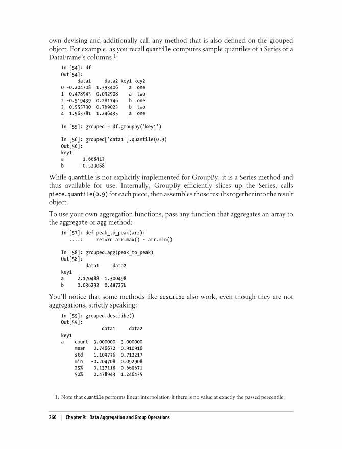
own devising and additionally call any method that is also defined on the groupedobject. For example, as you recall quantile computes sample quantiles of a Series or aDataFrame’s columns 1:
In [54]: dfOut[54]: data1 data2 key1 key20 -0.204708 1.393406 a one1 0.478943 0.092908 a two2 -0.519439 0.281746 b one3 -0.555730 0.769023 b two4 1.965781 1.246435 a one
In [55]: grouped = df.groupby('key1')
In [56]: grouped['data1'].quantile(0.9)Out[56]: key1a 1.668413b -0.523068
While quantile is not explicitly implemented for GroupBy, it is a Series method andthus available for use. Internally, GroupBy efficiently slices up the Series, callspiece.quantile(0.9) for each piece, then assembles those results together into the resultobject.
To use your own aggregation functions, pass any function that aggregates an array tothe aggregate or agg method:
In [57]: def peak_to_peak(arr): ....: return arr.max() - arr.min()
In [58]: grouped.agg(peak_to_peak)Out[58]: data1 data2key1 a 2.170488 1.300498b 0.036292 0.487276
You’ll notice that some methods like describe also work, even though they are notaggregations, strictly speaking:
In [59]: grouped.describe()Out[59]: data1 data2key1 a count 3.000000 3.000000 mean 0.746672 0.910916 std 1.109736 0.712217 min -0.204708 0.092908 25% 0.137118 0.669671 50% 0.478943 1.246435
1. Note that quantile performs linear interpolation if there is no value at exactly the passed percentile.
260 | Chapter 9: Data Aggregation and Group Operations

75% 1.222362 1.319920 max 1.965781 1.393406b count 2.000000 2.000000 mean -0.537585 0.525384 std 0.025662 0.344556 min -0.555730 0.281746 25% -0.546657 0.403565 50% -0.537585 0.525384 75% -0.528512 0.647203 max -0.519439 0.769023
I will explain in more detail what has happened here in the next major section on group-wise operations and transformations.
You may notice that custom aggregation functions are much slower thanthe optimized functions found in Table 9-1. This is because there issignificant overhead (function calls, data rearrangement) in construct-ing the intermediate group data chunks.
Table 9-1. Optimized groupby methods
Function name Description
count Number of non-NA values in the group
sum Sum of non-NA values
mean Mean of non-NA values
median Arithmetic median of non-NA values
std, var Unbiased (n - 1 denominator) standard deviation and variance
min, max Minimum and maximum of non-NA values
prod Product of non-NA values
first, last First and last non-NA values
To illustrate some more advanced aggregation features, I’ll use a less trivial dataset, adataset on restaurant tipping. I obtained it from the R reshape2 package; it was origi-nally found in Bryant & Smith’s 1995 text on business statistics (and found in the book’sGitHub repository). After loading it with read_csv, I add a tipping percentage columntip_pct.
In [60]: tips = pd.read_csv('ch08/tips.csv')
# Add tip percentage of total billIn [61]: tips['tip_pct'] = tips['tip'] / tips['total_bill']
In [62]: tips[:6]Out[62]: total_bill tip sex smoker day time size tip_pct0 16.99 1.01 Female No Sun Dinner 2 0.0594471 10.34 1.66 Male No Sun Dinner 3 0.160542
Data Aggregation | 261

2 21.01 3.50 Male No Sun Dinner 3 0.1665873 23.68 3.31 Male No Sun Dinner 2 0.1397804 24.59 3.61 Female No Sun Dinner 4 0.1468085 25.29 4.71 Male No Sun Dinner 4 0.186240
Column-wise and Multiple Function ApplicationAs you’ve seen above, aggregating a Series or all of the columns of a DataFrame is amatter of using aggregate with the desired function or calling a method like mean orstd. However, you may want to aggregate using a different function depending on thecolumn or multiple functions at once. Fortunately, this is straightforward to do, whichI’ll illustrate through a number of examples. First, I’ll group the tips by sex and smoker:
In [63]: grouped = tips.groupby(['sex', 'smoker'])
Note that for descriptive statistics like those in Table 9-1, you can pass the name of thefunction as a string:
In [64]: grouped_pct = grouped['tip_pct']
In [65]: grouped_pct.agg('mean')Out[65]: sex smokerFemale No 0.156921 Yes 0.182150Male No 0.160669 Yes 0.152771Name: tip_pct
If you pass a list of functions or function names instead, you get back a DataFrame withcolumn names taken from the functions:
In [66]: grouped_pct.agg(['mean', 'std', peak_to_peak])Out[66]: mean std peak_to_peaksex smoker Female No 0.156921 0.036421 0.195876 Yes 0.182150 0.071595 0.360233Male No 0.160669 0.041849 0.220186 Yes 0.152771 0.090588 0.674707
You don’t need to accept the names that GroupBy gives to the columns; notably lambda functions have the name '<lambda>' which make them hard to identify (you cansee for yourself by looking at a function’s __name__ attribute). As such, if you pass a listof (name, function) tuples, the first element of each tuple will be used as the DataFramecolumn names (you can think of a list of 2-tuples as an ordered mapping):
In [67]: grouped_pct.agg([('foo', 'mean'), ('bar', np.std)])Out[67]: foo barsex smoker Female No 0.156921 0.036421 Yes 0.182150 0.071595
262 | Chapter 9: Data Aggregation and Group Operations
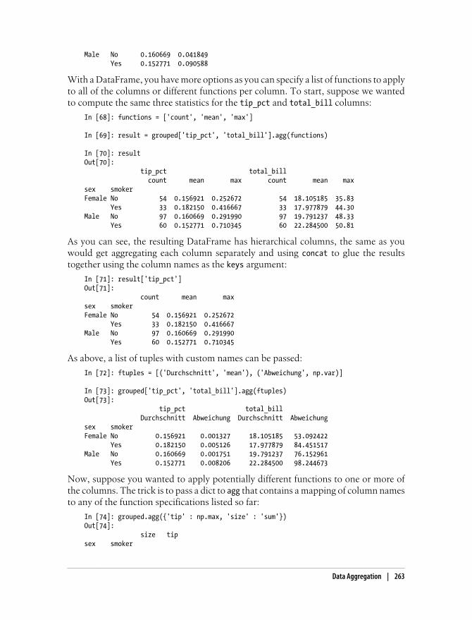
Male No 0.160669 0.041849 Yes 0.152771 0.090588
With a DataFrame, you have more options as you can specify a list of functions to applyto all of the columns or different functions per column. To start, suppose we wantedto compute the same three statistics for the tip_pct and total_bill columns:
In [68]: functions = ['count', 'mean', 'max']
In [69]: result = grouped['tip_pct', 'total_bill'].agg(functions)
In [70]: resultOut[70]: tip_pct total_bill count mean max count mean maxsex smoker Female No 54 0.156921 0.252672 54 18.105185 35.83 Yes 33 0.182150 0.416667 33 17.977879 44.30Male No 97 0.160669 0.291990 97 19.791237 48.33 Yes 60 0.152771 0.710345 60 22.284500 50.81
As you can see, the resulting DataFrame has hierarchical columns, the same as youwould get aggregating each column separately and using concat to glue the resultstogether using the column names as the keys argument:
In [71]: result['tip_pct']Out[71]: count mean maxsex smoker Female No 54 0.156921 0.252672 Yes 33 0.182150 0.416667Male No 97 0.160669 0.291990 Yes 60 0.152771 0.710345
As above, a list of tuples with custom names can be passed:
In [72]: ftuples = [('Durchschnitt', 'mean'), ('Abweichung', np.var)]
In [73]: grouped['tip_pct', 'total_bill'].agg(ftuples)Out[73]: tip_pct total_bill Durchschnitt Abweichung Durchschnitt Abweichungsex smoker Female No 0.156921 0.001327 18.105185 53.092422 Yes 0.182150 0.005126 17.977879 84.451517Male No 0.160669 0.001751 19.791237 76.152961 Yes 0.152771 0.008206 22.284500 98.244673
Now, suppose you wanted to apply potentially different functions to one or more ofthe columns. The trick is to pass a dict to agg that contains a mapping of column namesto any of the function specifications listed so far:
In [74]: grouped.agg({'tip' : np.max, 'size' : 'sum'})Out[74]: size tipsex smoker
Data Aggregation | 263

Female No 140 5.2 Yes 74 6.5Male No 263 9.0 Yes 150 10.0
In [75]: grouped.agg({'tip_pct' : ['min', 'max', 'mean', 'std'], ....: 'size' : 'sum'})Out[75]: tip_pct size min max mean std sumsex smoker Female No 0.056797 0.252672 0.156921 0.036421 140 Yes 0.056433 0.416667 0.182150 0.071595 74Male No 0.071804 0.291990 0.160669 0.041849 263 Yes 0.035638 0.710345 0.152771 0.090588 150
A DataFrame will have hierarchical columns only if multiple functions are applied toat least one column.
Returning Aggregated Data in “unindexed” FormIn all of the examples up until now, the aggregated data comes back with an index,potentially hierarchical, composed from the unique group key combinations observed.Since this isn’t always desirable, you can disable this behavior in most cases by passingas_index=False to groupby:
In [76]: tips.groupby(['sex', 'smoker'], as_index=False).mean()Out[76]: sex smoker total_bill tip size tip_pct0 Female No 18.105185 2.773519 2.592593 0.1569211 Female Yes 17.977879 2.931515 2.242424 0.1821502 Male No 19.791237 3.113402 2.711340 0.1606693 Male Yes 22.284500 3.051167 2.500000 0.152771
Of course, it’s always possible to obtain the result in this format by callingreset_index on the result.
Using groupby in this way is generally less flexible; results with hier-archical columns, for example, are not currently implemented as theform of the result would have to be somewhat arbitrary.
Group-wise Operations and TransformationsAggregation is only one kind of group operation. It is a special case in the more generalclass of data transformations; that is, it accepts functions that reduce a one-dimensionalarray to a scalar value. In this section, I will introduce you to the transform and applymethods, which will enable you to do many other kinds of group operations.
Suppose, instead, we wanted to add a column to a DataFrame containing group meansfor each index. One way to do this is to aggregate, then merge:
264 | Chapter 9: Data Aggregation and Group Operations
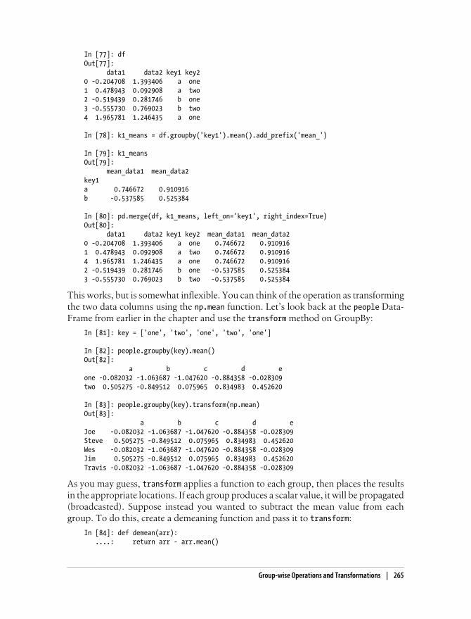
In [77]: dfOut[77]: data1 data2 key1 key20 -0.204708 1.393406 a one1 0.478943 0.092908 a two2 -0.519439 0.281746 b one3 -0.555730 0.769023 b two4 1.965781 1.246435 a one
In [78]: k1_means = df.groupby('key1').mean().add_prefix('mean_')
In [79]: k1_meansOut[79]: mean_data1 mean_data2key1 a 0.746672 0.910916b -0.537585 0.525384
In [80]: pd.merge(df, k1_means, left_on='key1', right_index=True)Out[80]: data1 data2 key1 key2 mean_data1 mean_data20 -0.204708 1.393406 a one 0.746672 0.9109161 0.478943 0.092908 a two 0.746672 0.9109164 1.965781 1.246435 a one 0.746672 0.9109162 -0.519439 0.281746 b one -0.537585 0.5253843 -0.555730 0.769023 b two -0.537585 0.525384
This works, but is somewhat inflexible. You can think of the operation as transformingthe two data columns using the np.mean function. Let’s look back at the people Data-Frame from earlier in the chapter and use the transform method on GroupBy:
In [81]: key = ['one', 'two', 'one', 'two', 'one']
In [82]: people.groupby(key).mean()Out[82]: a b c d eone -0.082032 -1.063687 -1.047620 -0.884358 -0.028309two 0.505275 -0.849512 0.075965 0.834983 0.452620
In [83]: people.groupby(key).transform(np.mean)Out[83]: a b c d eJoe -0.082032 -1.063687 -1.047620 -0.884358 -0.028309Steve 0.505275 -0.849512 0.075965 0.834983 0.452620Wes -0.082032 -1.063687 -1.047620 -0.884358 -0.028309Jim 0.505275 -0.849512 0.075965 0.834983 0.452620Travis -0.082032 -1.063687 -1.047620 -0.884358 -0.028309
As you may guess, transform applies a function to each group, then places the resultsin the appropriate locations. If each group produces a scalar value, it will be propagated(broadcasted). Suppose instead you wanted to subtract the mean value from eachgroup. To do this, create a demeaning function and pass it to transform:
In [84]: def demean(arr): ....: return arr - arr.mean()
Group-wise Operations and Transformations | 265
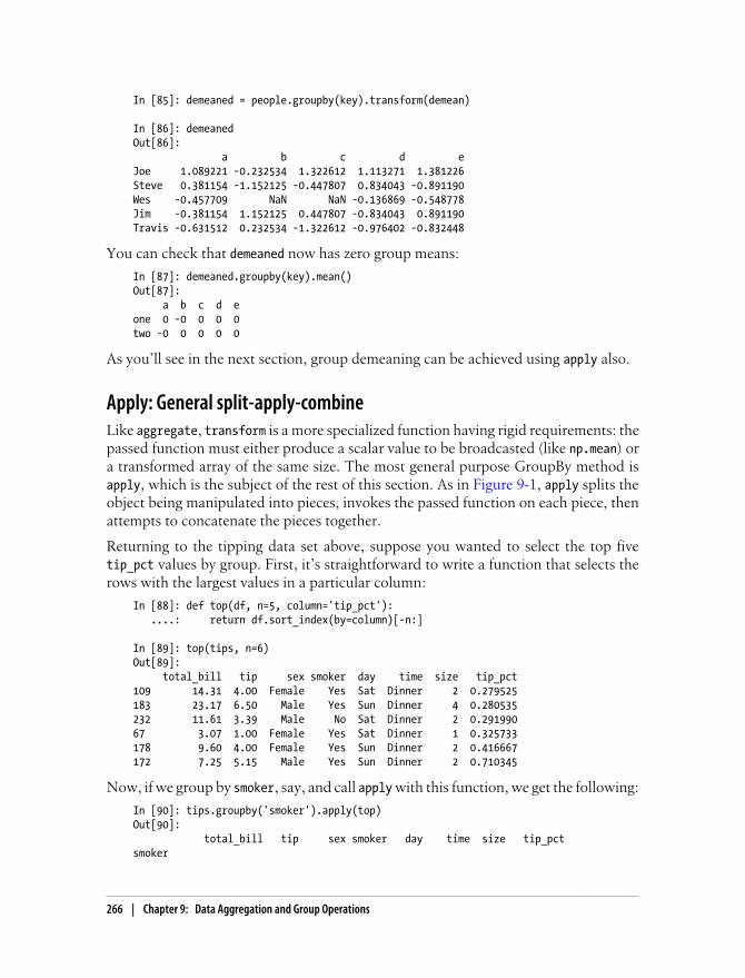
In [85]: demeaned = people.groupby(key).transform(demean)
In [86]: demeanedOut[86]: a b c d eJoe 1.089221 -0.232534 1.322612 1.113271 1.381226Steve 0.381154 -1.152125 -0.447807 0.834043 -0.891190Wes -0.457709 NaN NaN -0.136869 -0.548778Jim -0.381154 1.152125 0.447807 -0.834043 0.891190Travis -0.631512 0.232534 -1.322612 -0.976402 -0.832448
You can check that demeaned now has zero group means:
In [87]: demeaned.groupby(key).mean()Out[87]: a b c d eone 0 -0 0 0 0two -0 0 0 0 0
As you’ll see in the next section, group demeaning can be achieved using apply also.
Apply: General split-apply-combineLike aggregate, transform is a more specialized function having rigid requirements: thepassed function must either produce a scalar value to be broadcasted (like np.mean) ora transformed array of the same size. The most general purpose GroupBy method isapply, which is the subject of the rest of this section. As in Figure 9-1, apply splits theobject being manipulated into pieces, invokes the passed function on each piece, thenattempts to concatenate the pieces together.
Returning to the tipping data set above, suppose you wanted to select the top fivetip_pct values by group. First, it’s straightforward to write a function that selects therows with the largest values in a particular column:
In [88]: def top(df, n=5, column='tip_pct'): ....: return df.sort_index(by=column)[-n:]
In [89]: top(tips, n=6)Out[89]: total_bill tip sex smoker day time size tip_pct109 14.31 4.00 Female Yes Sat Dinner 2 0.279525183 23.17 6.50 Male Yes Sun Dinner 4 0.280535232 11.61 3.39 Male No Sat Dinner 2 0.29199067 3.07 1.00 Female Yes Sat Dinner 1 0.325733178 9.60 4.00 Female Yes Sun Dinner 2 0.416667172 7.25 5.15 Male Yes Sun Dinner 2 0.710345
Now, if we group by smoker, say, and call apply with this function, we get the following:
In [90]: tips.groupby('smoker').apply(top)Out[90]: total_bill tip sex smoker day time size tip_pctsmoker
266 | Chapter 9: Data Aggregation and Group Operations

No 88 24.71 5.85 Male No Thur Lunch 2 0.236746 185 20.69 5.00 Male No Sun Dinner 5 0.241663 51 10.29 2.60 Female No Sun Dinner 2 0.252672 149 7.51 2.00 Male No Thur Lunch 2 0.266312 232 11.61 3.39 Male No Sat Dinner 2 0.291990Yes 109 14.31 4.00 Female Yes Sat Dinner 2 0.279525 183 23.17 6.50 Male Yes Sun Dinner 4 0.280535 67 3.07 1.00 Female Yes Sat Dinner 1 0.325733 178 9.60 4.00 Female Yes Sun Dinner 2 0.416667 172 7.25 5.15 Male Yes Sun Dinner 2 0.710345
What has happened here? The top function is called on each piece of the DataFrame,then the results are glued together using pandas.concat, labeling the pieces with thegroup names. The result therefore has a hierarchical index whose inner level containsindex values from the original DataFrame.
If you pass a function to apply that takes other arguments or keywords, you can passthese after the function:
In [91]: tips.groupby(['smoker', 'day']).apply(top, n=1, column='total_bill')Out[91]: total_bill tip sex smoker day time size tip_pctsmoker day No Fri 94 22.75 3.25 Female No Fri Dinner 2 0.142857 Sat 212 48.33 9.00 Male No Sat Dinner 4 0.186220 Sun 156 48.17 5.00 Male No Sun Dinner 6 0.103799 Thur 142 41.19 5.00 Male No Thur Lunch 5 0.121389Yes Fri 95 40.17 4.73 Male Yes Fri Dinner 4 0.117750 Sat 170 50.81 10.00 Male Yes Sat Dinner 3 0.196812 Sun 182 45.35 3.50 Male Yes Sun Dinner 3 0.077178 Thur 197 43.11 5.00 Female Yes Thur Lunch 4 0.115982
Beyond these basic usage mechanics, getting the most out of apply islargely a matter of creativity. What occurs inside the function passed isup to you; it only needs to return a pandas object or a scalar value. Therest of this chapter will mainly consist of examples showing you how tosolve various problems using groupby.
You may recall above I called describe on a GroupBy object:
In [92]: result = tips.groupby('smoker')['tip_pct'].describe()
In [93]: resultOut[93]: smoker No count 151.000000 mean 0.159328 std 0.039910 min 0.056797 25% 0.136906 50% 0.155625 75% 0.185014 max 0.291990
Group-wise Operations and Transformations | 267

Yes count 93.000000 mean 0.163196 std 0.085119 min 0.035638 25% 0.106771 50% 0.153846 75% 0.195059 max 0.710345
In [94]: result.unstack('smoker')Out[94]: smoker No Yescount 151.000000 93.000000mean 0.159328 0.163196std 0.039910 0.085119min 0.056797 0.03563825% 0.136906 0.10677150% 0.155625 0.15384675% 0.185014 0.195059max 0.291990 0.710345
Inside GroupBy, when you invoke a method like describe, it is actually just a shortcutfor:
f = lambda x: x.describe()grouped.apply(f)
Suppressing the group keys
In the examples above, you see that the resulting object has a hierarchical index formedfrom the group keys along with the indexes of each piece of the original object. Thiscan be disabled by passing group_keys=False to groupby:
In [95]: tips.groupby('smoker', group_keys=False).apply(top)Out[95]: total_bill tip sex smoker day time size tip_pct88 24.71 5.85 Male No Thur Lunch 2 0.236746185 20.69 5.00 Male No Sun Dinner 5 0.24166351 10.29 2.60 Female No Sun Dinner 2 0.252672149 7.51 2.00 Male No Thur Lunch 2 0.266312232 11.61 3.39 Male No Sat Dinner 2 0.291990109 14.31 4.00 Female Yes Sat Dinner 2 0.279525183 23.17 6.50 Male Yes Sun Dinner 4 0.28053567 3.07 1.00 Female Yes Sat Dinner 1 0.325733178 9.60 4.00 Female Yes Sun Dinner 2 0.416667172 7.25 5.15 Male Yes Sun Dinner 2 0.710345
Quantile and Bucket AnalysisAs you may recall from Chapter 7, pandas has some tools, in particular cut and qcut,for slicing data up into buckets with bins of your choosing or by sample quantiles.Combining these functions with groupby, it becomes very simple to perform bucket or
268 | Chapter 9: Data Aggregation and Group Operations

quantile analysis on a data set. Consider a simple random data set and an equal-lengthbucket categorization using cut:
In [96]: frame = DataFrame({'data1': np.random.randn(1000), ....: 'data2': np.random.randn(1000)})
In [97]: factor = pd.cut(frame.data1, 4)
In [98]: factor[:10]Out[98]: Categorical: array([(-1.23, 0.489], (-2.956, -1.23], (-1.23, 0.489], (0.489, 2.208], (-1.23, 0.489], (0.489, 2.208], (-1.23, 0.489], (-1.23, 0.489], (0.489, 2.208], (0.489, 2.208]], dtype=object)Levels (4): Index([(-2.956, -1.23], (-1.23, 0.489], (0.489, 2.208], (2.208, 3.928]], dtype=object)
The Factor object returned by cut can be passed directly to groupby. So we could com-pute a set of statistics for the data2 column like so:
In [99]: def get_stats(group): ....: return {'min': group.min(), 'max': group.max(), ....: 'count': group.count(), 'mean': group.mean()}
In [100]: grouped = frame.data2.groupby(factor)
In [101]: grouped.apply(get_stats).unstack()Out[101]: count max mean mindata1 (-1.23, 0.489] 598 3.260383 -0.002051 -2.989741(-2.956, -1.23] 95 1.670835 -0.039521 -3.399312(0.489, 2.208] 297 2.954439 0.081822 -3.745356(2.208, 3.928] 10 1.765640 0.024750 -1.929776
These were equal-length buckets; to compute equal-size buckets based on samplequantiles, use qcut. I’ll pass labels=False to just get quantile numbers.
# Return quantile numbersIn [102]: grouping = pd.qcut(frame.data1, 10, labels=False)
In [103]: grouped = frame.data2.groupby(grouping)
In [104]: grouped.apply(get_stats).unstack()Out[104]: count max mean min0 100 1.670835 -0.049902 -3.3993121 100 2.628441 0.030989 -1.9500982 100 2.527939 -0.067179 -2.9251133 100 3.260383 0.065713 -2.3155554 100 2.074345 -0.111653 -2.0479395 100 2.184810 0.052130 -2.9897416 100 2.458842 -0.021489 -2.2235067 100 2.954439 -0.026459 -3.0569908 100 2.735527 0.103406 -3.7453569 100 2.377020 0.220122 -2.064111
Group-wise Operations and Transformations | 269

Example: Filling Missing Values with Group-specific ValuesWhen cleaning up missing data, in some cases you will filter out data observationsusing dropna, but in others you may want to impute (fill in) the NA values using a fixedvalue or some value derived from the data. fillna is the right tool to use; for examplehere I fill in NA values with the mean:
In [105]: s = Series(np.random.randn(6))
In [106]: s[::2] = np.nan
In [107]: sOut[107]: 0 NaN1 -0.1259212 NaN3 -0.8844754 NaN5 0.227290
In [108]: s.fillna(s.mean())Out[108]: 0 -0.2610351 -0.1259212 -0.2610353 -0.8844754 -0.2610355 0.227290
Suppose you need the fill value to vary by group. As you may guess, you need onlygroup the data and use apply with a function that calls fillna on each data chunk. Hereis some sample data on some US states divided into eastern and western states:
In [109]: states = ['Ohio', 'New York', 'Vermont', 'Florida', .....: 'Oregon', 'Nevada', 'California', 'Idaho']
In [110]: group_key = ['East'] * 4 + ['West'] * 4
In [111]: data = Series(np.random.randn(8), index=states)
In [112]: data[['Vermont', 'Nevada', 'Idaho']] = np.nan
In [113]: dataOut[113]: Ohio 0.922264New York -2.153545Vermont NaNFlorida -0.375842Oregon 0.329939Nevada NaNCalifornia 1.105913Idaho NaN
In [114]: data.groupby(group_key).mean()Out[114]:
270 | Chapter 9: Data Aggregation and Group Operations
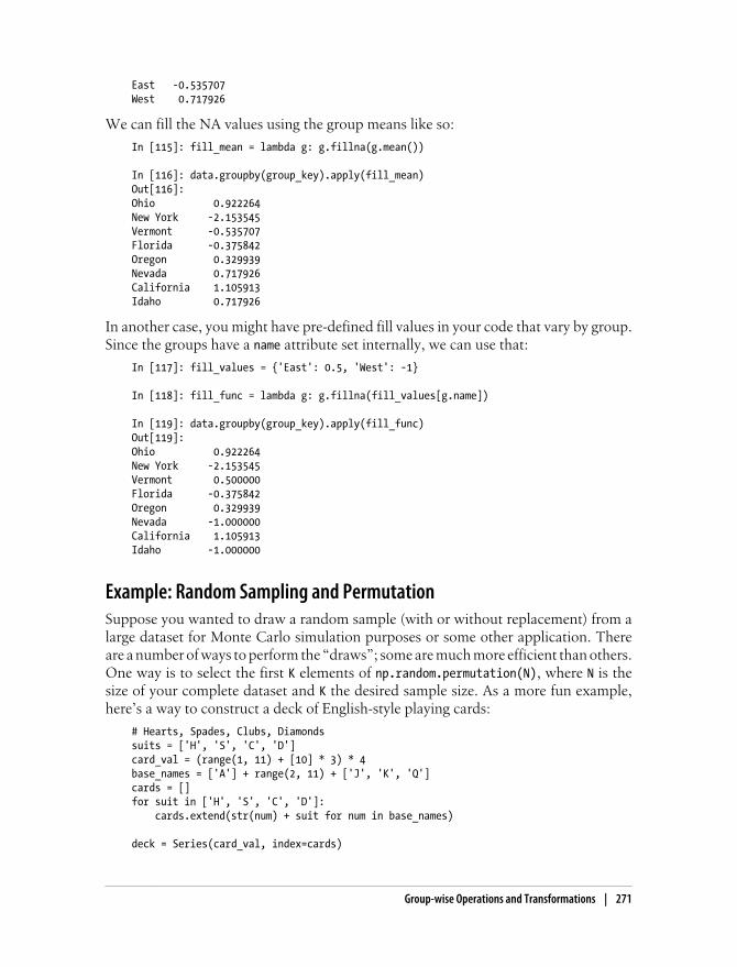
East -0.535707West 0.717926
We can fill the NA values using the group means like so:
In [115]: fill_mean = lambda g: g.fillna(g.mean())
In [116]: data.groupby(group_key).apply(fill_mean)Out[116]: Ohio 0.922264New York -2.153545Vermont -0.535707Florida -0.375842Oregon 0.329939Nevada 0.717926California 1.105913Idaho 0.717926
In another case, you might have pre-defined fill values in your code that vary by group.Since the groups have a name attribute set internally, we can use that:
In [117]: fill_values = {'East': 0.5, 'West': -1}
In [118]: fill_func = lambda g: g.fillna(fill_values[g.name])
In [119]: data.groupby(group_key).apply(fill_func)Out[119]: Ohio 0.922264New York -2.153545Vermont 0.500000Florida -0.375842Oregon 0.329939Nevada -1.000000California 1.105913Idaho -1.000000
Example: Random Sampling and PermutationSuppose you wanted to draw a random sample (with or without replacement) from alarge dataset for Monte Carlo simulation purposes or some other application. Thereare a number of ways to perform the “draws”; some are much more efficient than others.One way is to select the first K elements of np.random.permutation(N), where N is thesize of your complete dataset and K the desired sample size. As a more fun example,here’s a way to construct a deck of English-style playing cards:
# Hearts, Spades, Clubs, Diamondssuits = ['H', 'S', 'C', 'D']card_val = (range(1, 11) + [10] * 3) * 4base_names = ['A'] + range(2, 11) + ['J', 'K', 'Q']cards = []for suit in ['H', 'S', 'C', 'D']: cards.extend(str(num) + suit for num in base_names)
deck = Series(card_val, index=cards)
Group-wise Operations and Transformations | 271

So now we have a Series of length 52 whose index contains card names and values arethe ones used in blackjack and other games (to keep things simple, I just let the ace be1):
In [121]: deck[:13]Out[121]: AH 12H 23H 34H 45H 56H 67H 78H 89H 910H 10JH 10KH 10QH 10
Now, based on what I said above, drawing a hand of 5 cards from the desk could bewritten as:
In [122]: def draw(deck, n=5): .....: return deck.take(np.random.permutation(len(deck))[:n])
In [123]: draw(deck)Out[123]: AD 18C 85H 5KC 102C 2
Suppose you wanted two random cards from each suit. Because the suit is the lastcharacter of each card name, we can group based on this and use apply:
In [124]: get_suit = lambda card: card[-1] # last letter is suit
In [125]: deck.groupby(get_suit).apply(draw, n=2)Out[125]: C 2C 2 3C 3D KD 10 8D 8H KH 10 3H 3S 2S 2 4S 4
# alternativelyIn [126]: deck.groupby(get_suit, group_keys=False).apply(draw, n=2)Out[126]: KC 10JC 10AD 1
272 | Chapter 9: Data Aggregation and Group Operations

5D 55H 56H 67S 7KS 10
Example: Group Weighted Average and CorrelationUnder the split-apply-combine paradigm of groupby, operations between columns in aDataFrame or two Series, such a group weighted average, become a routine affair. Asan example, take this dataset containing group keys, values, and some weights:
In [127]: df = DataFrame({'category': ['a', 'a', 'a', 'a', 'b', 'b', 'b', 'b'], .....: 'data': np.random.randn(8), .....: 'weights': np.random.rand(8)})
In [128]: dfOut[128]: category data weights0 a 1.561587 0.9575151 a 1.219984 0.3472672 a -0.482239 0.5813623 a 0.315667 0.2170914 b -0.047852 0.8944065 b -0.454145 0.9185646 b -0.556774 0.2778257 b 0.253321 0.955905
The group weighted average by category would then be:
In [129]: grouped = df.groupby('category')
In [130]: get_wavg = lambda g: np.average(g['data'], weights=g['weights'])
In [131]: grouped.apply(get_wavg)Out[131]: categorya 0.811643b -0.122262
As a less trivial example, consider a data set from Yahoo! Finance containing end ofday prices for a few stocks and the S&P 500 index (the SPX ticker):
In [132]: close_px = pd.read_csv('ch09/stock_px.csv', parse_dates=True, index_col=0)
In [133]: close_pxOut[133]: <class 'pandas.core.frame.DataFrame'>DatetimeIndex: 2214 entries, 2003-01-02 00:00:00 to 2011-10-14 00:00:00Data columns:AAPL 2214 non-null valuesMSFT 2214 non-null valuesXOM 2214 non-null valuesSPX 2214 non-null valuesdtypes: float64(4)
Group-wise Operations and Transformations | 273

In [134]: close_px[-4:]Out[134]: AAPL MSFT XOM SPX2011-10-11 400.29 27.00 76.27 1195.542011-10-12 402.19 26.96 77.16 1207.252011-10-13 408.43 27.18 76.37 1203.662011-10-14 422.00 27.27 78.11 1224.58
One task of interest might be to compute a DataFrame consisting of the yearly corre-lations of daily returns (computed from percent changes) with SPX. Here is one way todo it:
In [135]: rets = close_px.pct_change().dropna()
In [136]: spx_corr = lambda x: x.corrwith(x['SPX'])
In [137]: by_year = rets.groupby(lambda x: x.year)
In [138]: by_year.apply(spx_corr)Out[138]: AAPL MSFT XOM SPX2003 0.541124 0.745174 0.661265 12004 0.374283 0.588531 0.557742 12005 0.467540 0.562374 0.631010 12006 0.428267 0.406126 0.518514 12007 0.508118 0.658770 0.786264 12008 0.681434 0.804626 0.828303 12009 0.707103 0.654902 0.797921 12010 0.710105 0.730118 0.839057 12011 0.691931 0.800996 0.859975 1
There is, of course, nothing to stop you from computing inter-column correlations:
# Annual correlation of Apple with MicrosoftIn [139]: by_year.apply(lambda g: g['AAPL'].corr(g['MSFT']))Out[139]: 2003 0.4808682004 0.2590242005 0.3000932006 0.1617352007 0.4177382008 0.6119012009 0.4327382010 0.5719462011 0.581987
Example: Group-wise Linear RegressionIn the same vein as the previous example, you can use groupby to perform more complexgroup-wise statistical analysis, as long as the function returns a pandas object or scalarvalue. For example, I can define the following regress function (using the statsmodels econometrics library) which executes an ordinary least squares (OLS) regressionon each chunk of data:
274 | Chapter 9: Data Aggregation and Group Operations

import statsmodels.api as smdef regress(data, yvar, xvars): Y = data[yvar] X = data[xvars] X['intercept'] = 1. result = sm.OLS(Y, X).fit() return result.params
Now, to run a yearly linear regression of AAPL on SPX returns, I execute:
In [141]: by_year.apply(regress, 'AAPL', ['SPX'])Out[141]: SPX intercept2003 1.195406 0.0007102004 1.363463 0.0042012005 1.766415 0.0032462006 1.645496 0.0000802007 1.198761 0.0034382008 0.968016 -0.0011102009 0.879103 0.0029542010 1.052608 0.0012612011 0.806605 0.001514
Pivot Tables and Cross-TabulationA pivot table is a data summarization tool frequently found in spreadsheet programsand other data analysis software. It aggregates a table of data by one or more keys,arranging the data in a rectangle with some of the group keys along the rows and somealong the columns. Pivot tables in Python with pandas are made possible using thegroupby facility described in this chapter combined with reshape operations utilizinghierarchical indexing. DataFrame has a pivot_table method, and additionally there isa top-level pandas.pivot_table function. In addition to providing a convenience inter-face to groupby, pivot_table also can add partial totals, also known as margins.
Returning to the tipping data set, suppose I wanted to compute a table of group means(the default pivot_table aggregation type) arranged by sex and smoker on the rows:
In [142]: tips.pivot_table(rows=['sex', 'smoker'])Out[142]: size tip tip_pct total_billsex smoker Female No 2.592593 2.773519 0.156921 18.105185 Yes 2.242424 2.931515 0.182150 17.977879Male No 2.711340 3.113402 0.160669 19.791237 Yes 2.500000 3.051167 0.152771 22.284500
This could have been easily produced using groupby. Now, suppose we want to aggre-gate only tip_pct and size, and additionally group by day. I’ll put smoker in the tablecolumns and day in the rows:
In [143]: tips.pivot_table(['tip_pct', 'size'], rows=['sex', 'day'], .....: cols='smoker')Out[143]:
Pivot Tables and Cross-Tabulation | 275
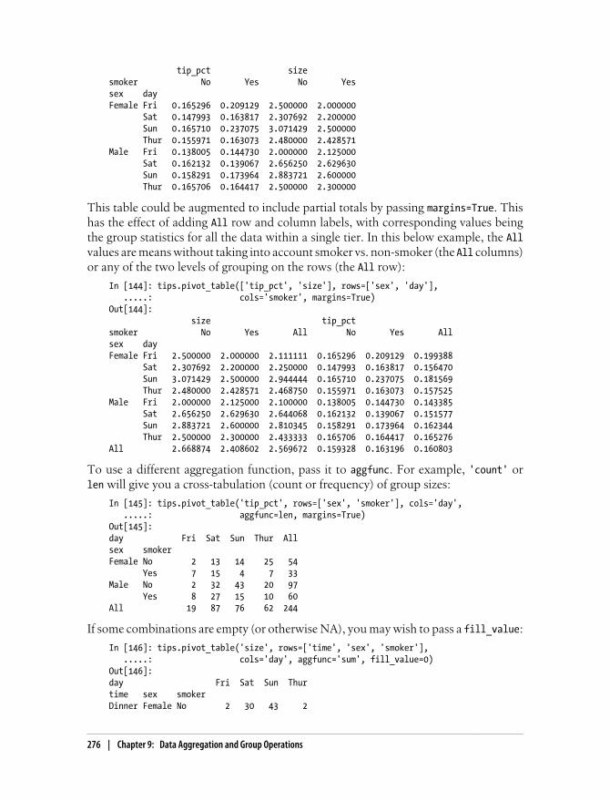
tip_pct size smoker No Yes No Yessex day Female Fri 0.165296 0.209129 2.500000 2.000000 Sat 0.147993 0.163817 2.307692 2.200000 Sun 0.165710 0.237075 3.071429 2.500000 Thur 0.155971 0.163073 2.480000 2.428571Male Fri 0.138005 0.144730 2.000000 2.125000 Sat 0.162132 0.139067 2.656250 2.629630 Sun 0.158291 0.173964 2.883721 2.600000 Thur 0.165706 0.164417 2.500000 2.300000
This table could be augmented to include partial totals by passing margins=True. Thishas the effect of adding All row and column labels, with corresponding values beingthe group statistics for all the data within a single tier. In this below example, the Allvalues are means without taking into account smoker vs. non-smoker (the All columns)or any of the two levels of grouping on the rows (the All row):
In [144]: tips.pivot_table(['tip_pct', 'size'], rows=['sex', 'day'], .....: cols='smoker', margins=True)Out[144]: size tip_pct smoker No Yes All No Yes Allsex day Female Fri 2.500000 2.000000 2.111111 0.165296 0.209129 0.199388 Sat 2.307692 2.200000 2.250000 0.147993 0.163817 0.156470 Sun 3.071429 2.500000 2.944444 0.165710 0.237075 0.181569 Thur 2.480000 2.428571 2.468750 0.155971 0.163073 0.157525Male Fri 2.000000 2.125000 2.100000 0.138005 0.144730 0.143385 Sat 2.656250 2.629630 2.644068 0.162132 0.139067 0.151577 Sun 2.883721 2.600000 2.810345 0.158291 0.173964 0.162344 Thur 2.500000 2.300000 2.433333 0.165706 0.164417 0.165276All 2.668874 2.408602 2.569672 0.159328 0.163196 0.160803
To use a different aggregation function, pass it to aggfunc. For example, 'count' orlen will give you a cross-tabulation (count or frequency) of group sizes:
In [145]: tips.pivot_table('tip_pct', rows=['sex', 'smoker'], cols='day', .....: aggfunc=len, margins=True)Out[145]: day Fri Sat Sun Thur Allsex smoker Female No 2 13 14 25 54 Yes 7 15 4 7 33Male No 2 32 43 20 97 Yes 8 27 15 10 60All 19 87 76 62 244
If some combinations are empty (or otherwise NA), you may wish to pass a fill_value:
In [146]: tips.pivot_table('size', rows=['time', 'sex', 'smoker'], .....: cols='day', aggfunc='sum', fill_value=0)Out[146]: day Fri Sat Sun Thurtime sex smoker Dinner Female No 2 30 43 2
276 | Chapter 9: Data Aggregation and Group Operations
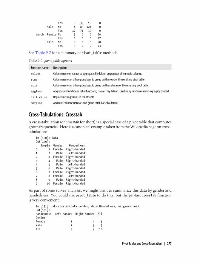
Yes 8 33 10 0 Male No 4 85 124 0 Yes 12 71 39 0Lunch Female No 3 0 0 60 Yes 6 0 0 17 Male No 0 0 0 50 Yes 5 0 0 23
See Table 9-2 for a summary of pivot_table methods.
Table 9-2. pivot_table options
Function name Description
values Column name or names to aggregate. By default aggregates all numeric columns
rows Column names or other group keys to group on the rows of the resulting pivot table
cols Column names or other group keys to group on the columns of the resulting pivot table
aggfunc Aggregation function or list of functions; 'mean' by default. Can be any function valid in a groupby context
fill_value Replace missing values in result table
margins Add row/column subtotals and grand total, False by default
Cross-Tabulations: CrosstabA cross-tabulation (or crosstab for short) is a special case of a pivot table that computesgroup frequencies. Here is a canonical example taken from the Wikipedia page on cross-tabulation:
In [150]: dataOut[150]: Sample Gender Handedness0 1 Female Right-handed1 2 Male Left-handed2 3 Female Right-handed3 4 Male Right-handed4 5 Male Left-handed5 6 Male Right-handed6 7 Female Right-handed7 8 Female Left-handed8 9 Male Right-handed9 10 Female Right-handed
As part of some survey analysis, we might want to summarize this data by gender andhandedness. You could use pivot_table to do this, but the pandas.crosstab functionis very convenient:
In [151]: pd.crosstab(data.Gender, data.Handedness, margins=True)Out[151]: Handedness Left-handed Right-handed AllGender Female 1 4 5Male 2 3 5All 3 7 10
Pivot Tables and Cross-Tabulation | 277

The first two arguments to crosstab can each either be an array or Series or a list ofarrays. As in the tips data:
In [152]: pd.crosstab([tips.time, tips.day], tips.smoker, margins=True)Out[152]: smoker No Yes Alltime day Dinner Fri 3 9 12 Sat 45 42 87 Sun 57 19 76 Thur 1 0 1Lunch Fri 1 6 7 Thur 44 17 61All 151 93 244
Example: 2012 Federal Election Commission DatabaseThe US Federal Election Commission publishes data on contributions to political cam-paigns. This includes contributor names, occupation and employer, address, and con-tribution amount. An interesting dataset is from the 2012 US presidential election(http://www.fec.gov/disclosurep/PDownload.do). As of this writing (June 2012), the fulldataset for all states is a 150 megabyte CSV file P00000001-ALL.csv, which can be loadedwith pandas.read_csv:
In [13]: fec = pd.read_csv('ch09/P00000001-ALL.csv')
In [14]: fecOut[14]:<class 'pandas.core.frame.DataFrame'>Int64Index: 1001731 entries, 0 to 1001730Data columns:cmte_id 1001731 non-null valuescand_id 1001731 non-null valuescand_nm 1001731 non-null valuescontbr_nm 1001731 non-null valuescontbr_city 1001716 non-null valuescontbr_st 1001727 non-null valuescontbr_zip 1001620 non-null valuescontbr_employer 994314 non-null valuescontbr_occupation 994433 non-null valuescontb_receipt_amt 1001731 non-null valuescontb_receipt_dt 1001731 non-null valuesreceipt_desc 14166 non-null valuesmemo_cd 92482 non-null valuesmemo_text 97770 non-null valuesform_tp 1001731 non-null valuesfile_num 1001731 non-null valuesdtypes: float64(1), int64(1), object(14)
A sample record in the DataFrame looks like this:
In [15]: fec.ix[123456]Out[15]:cmte_id C00431445
278 | Chapter 9: Data Aggregation and Group Operations

cand_id P80003338cand_nm Obama, Barackcontbr_nm ELLMAN, IRAcontbr_city TEMPEcontbr_st AZcontbr_zip 852816719contbr_employer ARIZONA STATE UNIVERSITYcontbr_occupation PROFESSORcontb_receipt_amt 50contb_receipt_dt 01-DEC-11receipt_desc NaNmemo_cd NaNmemo_text NaNform_tp SA17Afile_num 772372Name: 123456
You can probably think of many ways to start slicing and dicing this data to extractinformative statistics about donors and patterns in the campaign contributions. I’llspend the next several pages showing you a number of different analyses that applytechniques you have learned about so far.
You can see that there are no political party affiliations in the data, so this would beuseful to add. You can get a list of all the unique political candidates using unique (notethat NumPy suppresses the quotes around the strings in the output):
In [16]: unique_cands = fec.cand_nm.unique()
In [17]: unique_candsOut[17]:array([Bachmann, Michelle, Romney, Mitt, Obama, Barack, Roemer, Charles E. 'Buddy' III, Pawlenty, Timothy, Johnson, Gary Earl, Paul, Ron, Santorum, Rick, Cain, Herman, Gingrich, Newt, McCotter, Thaddeus G, Huntsman, Jon, Perry, Rick], dtype=object)
In [18]: unique_cands[2]Out[18]: 'Obama, Barack'
An easy way to indicate party affiliation is using a dict:2
parties = {'Bachmann, Michelle': 'Republican', 'Cain, Herman': 'Republican', 'Gingrich, Newt': 'Republican', 'Huntsman, Jon': 'Republican', 'Johnson, Gary Earl': 'Republican', 'McCotter, Thaddeus G': 'Republican', 'Obama, Barack': 'Democrat', 'Paul, Ron': 'Republican', 'Pawlenty, Timothy': 'Republican', 'Perry, Rick': 'Republican', "Roemer, Charles E. 'Buddy' III": 'Republican',
2. This makes the simplifying assumption that Gary Johnson is a Republican even though he later becamethe Libertarian party candidate.
Example: 2012 Federal Election Commission Database | 279

'Romney, Mitt': 'Republican', 'Santorum, Rick': 'Republican'}
Now, using this mapping and the map method on Series objects, you can compute anarray of political parties from the candidate names:
In [20]: fec.cand_nm[123456:123461]Out[20]:123456 Obama, Barack123457 Obama, Barack123458 Obama, Barack123459 Obama, Barack123460 Obama, BarackName: cand_nm
In [21]: fec.cand_nm[123456:123461].map(parties)Out[21]:123456 Democrat123457 Democrat123458 Democrat123459 Democrat123460 DemocratName: cand_nm
# Add it as a columnIn [22]: fec['party'] = fec.cand_nm.map(parties)
In [23]: fec['party'].value_counts()Out[23]:Democrat 593746Republican 407985
A couple of data preparation points. First, this data includes both contributions andrefunds (negative contribution amount):
In [24]: (fec.contb_receipt_amt > 0).value_counts()Out[24]:True 991475False 10256
To simplify the analysis, I’ll restrict the data set to positive contributions:
In [25]: fec = fec[fec.contb_receipt_amt > 0]
Since Barack Obama and Mitt Romney are the main two candidates, I’ll also preparea subset that just has contributions to their campaigns:
In [26]: fec_mrbo = fec[fec.cand_nm.isin(['Obama, Barack', 'Romney, Mitt'])]
Donation Statistics by Occupation and EmployerDonations by occupation is another oft-studied statistic. For example, lawyers (attor-neys) tend to donate more money to Democrats, while business executives tend todonate more to Republicans. You have no reason to believe me; you can see for yourselfin the data. First, the total number of donations by occupation is easy:
280 | Chapter 9: Data Aggregation and Group Operations

In [27]: fec.contbr_occupation.value_counts()[:10]Out[27]:RETIRED 233990INFORMATION REQUESTED 35107ATTORNEY 34286HOMEMAKER 29931PHYSICIAN 23432INFORMATION REQUESTED PER BEST EFFORTS 21138ENGINEER 14334TEACHER 13990CONSULTANT 13273PROFESSOR 12555
You will notice by looking at the occupations that many refer to the same basic jobtype, or there are several variants of the same thing. Here is a code snippet illustrates atechnique for cleaning up a few of them by mapping from one occupation to another;note the “trick” of using dict.get to allow occupations with no mapping to “passthrough”:
occ_mapping = { 'INFORMATION REQUESTED PER BEST EFFORTS' : 'NOT PROVIDED', 'INFORMATION REQUESTED' : 'NOT PROVIDED', 'INFORMATION REQUESTED (BEST EFFORTS)' : 'NOT PROVIDED', 'C.E.O.': 'CEO'}
# If no mapping provided, return xf = lambda x: occ_mapping.get(x, x)fec.contbr_occupation = fec.contbr_occupation.map(f)
I’ll also do the same thing for employers:
emp_mapping = { 'INFORMATION REQUESTED PER BEST EFFORTS' : 'NOT PROVIDED', 'INFORMATION REQUESTED' : 'NOT PROVIDED', 'SELF' : 'SELF-EMPLOYED', 'SELF EMPLOYED' : 'SELF-EMPLOYED',}
# If no mapping provided, return xf = lambda x: emp_mapping.get(x, x)fec.contbr_employer = fec.contbr_employer.map(f)
Now, you can use pivot_table to aggregate the data by party and occupation, thenfilter down to the subset that donated at least $2 million overall:
In [34]: by_occupation = fec.pivot_table('contb_receipt_amt', ....: rows='contbr_occupation', ....: cols='party', aggfunc='sum')
In [35]: over_2mm = by_occupation[by_occupation.sum(1) > 2000000]
In [36]: over_2mmOut[36]:party Democrat Republicancontbr_occupation
Example: 2012 Federal Election Commission Database | 281

ATTORNEY 11141982.97 7477194.430000CEO 2074974.79 4211040.520000CONSULTANT 2459912.71 2544725.450000ENGINEER 951525.55 1818373.700000EXECUTIVE 1355161.05 4138850.090000HOMEMAKER 4248875.80 13634275.780000INVESTOR 884133.00 2431768.920000LAWYER 3160478.87 391224.320000MANAGER 762883.22 1444532.370000NOT PROVIDED 4866973.96 20565473.010000OWNER 1001567.36 2408286.920000PHYSICIAN 3735124.94 3594320.240000PRESIDENT 1878509.95 4720923.760000PROFESSOR 2165071.08 296702.730000REAL ESTATE 528902.09 1625902.250000RETIRED 25305116.38 23561244.489999SELF-EMPLOYED 672393.40 1640252.540000
It can be easier to look at this data graphically as a bar plot ('barh' means horizontalbar plot, see Figure 9-2):
In [38]: over_2mm.plot(kind='barh')
Figure 9-2. Total donations by party for top occupations
You might be interested in the top donor occupations or top companies donating toObama and Romney. To do this, you can group by candidate name and use a variantof the top method from earlier in the chapter:
def get_top_amounts(group, key, n=5): totals = group.groupby(key)['contb_receipt_amt'].sum()
# Order totals by key in descending order return totals.order(ascending=False)[-n:]
282 | Chapter 9: Data Aggregation and Group Operations

Then aggregated by occupation and employer:
In [40]: grouped = fec_mrbo.groupby('cand_nm')
In [41]: grouped.apply(get_top_amounts, 'contbr_occupation', n=7)Out[41]:cand_nm contbr_occupationObama, Barack RETIRED 25305116.38 ATTORNEY 11141982.97 NOT PROVIDED 4866973.96 HOMEMAKER 4248875.80 PHYSICIAN 3735124.94 LAWYER 3160478.87 CONSULTANT 2459912.71Romney, Mitt RETIRED 11508473.59 NOT PROVIDED 11396894.84 HOMEMAKER 8147446.22 ATTORNEY 5364718.82 PRESIDENT 2491244.89 EXECUTIVE 2300947.03 C.E.O. 1968386.11Name: contb_receipt_amt
In [42]: grouped.apply(get_top_amounts, 'contbr_employer', n=10)Out[42]:cand_nm contbr_employerObama, Barack RETIRED 22694358.85 SELF-EMPLOYED 18626807.16 NOT EMPLOYED 8586308.70 NOT PROVIDED 5053480.37 HOMEMAKER 2605408.54 STUDENT 318831.45 VOLUNTEER 257104.00 MICROSOFT 215585.36 SIDLEY AUSTIN LLP 168254.00 REFUSED 149516.07Romney, Mitt NOT PROVIDED 12059527.24 RETIRED 11506225.71 HOMEMAKER 8147196.22 SELF-EMPLOYED 7414115.22 STUDENT 496490.94 CREDIT SUISSE 281150.00 MORGAN STANLEY 267266.00 GOLDMAN SACH & CO. 238250.00 BARCLAYS CAPITAL 162750.00 H.I.G. CAPITAL 139500.00Name: contb_receipt_amt
Bucketing Donation AmountsA useful way to analyze this data is to use the cut function to discretize the contributoramounts into buckets by contribution size:
In [43]: bins = np.array([0, 1, 10, 100, 1000, 10000, 100000, 1000000, 10000000])
Example: 2012 Federal Election Commission Database | 283

In [44]: labels = pd.cut(fec_mrbo.contb_receipt_amt, bins)
In [45]: labelsOut[45]:Categorical:contb_receipt_amtarray([(10, 100], (100, 1000], (100, 1000], ..., (1, 10], (10, 100], (100, 1000]], dtype=object)Levels (8): array([(0, 1], (1, 10], (10, 100], (100, 1000], (1000, 10000], (10000, 100000], (100000, 1000000], (1000000, 10000000]], dtype=object)
We can then group the data for Obama and Romney by name and bin label to get ahistogram by donation size:
In [46]: grouped = fec_mrbo.groupby(['cand_nm', labels])
In [47]: grouped.size().unstack(0)Out[47]:cand_nm Obama, Barack Romney, Mittcontb_receipt_amt(0, 1] 493 77(1, 10] 40070 3681(10, 100] 372280 31853(100, 1000] 153991 43357(1000, 10000] 22284 26186(10000, 100000] 2 1(100000, 1000000] 3 NaN(1000000, 10000000] 4 NaN
This data shows that Obama has received a significantly larger number of small don-ations than Romney. You can also sum the contribution amounts and normalize withinbuckets to visualize percentage of total donations of each size by candidate:
In [48]: bucket_sums = grouped.contb_receipt_amt.sum().unstack(0)
In [49]: bucket_sumsOut[49]:cand_nm Obama, Barack Romney, Mittcontb_receipt_amt(0, 1] 318.24 77.00(1, 10] 337267.62 29819.66(10, 100] 20288981.41 1987783.76(100, 1000] 54798531.46 22363381.69(1000, 10000] 51753705.67 63942145.42(10000, 100000] 59100.00 12700.00(100000, 1000000] 1490683.08 NaN(1000000, 10000000] 7148839.76 NaN
In [50]: normed_sums = bucket_sums.div(bucket_sums.sum(axis=1), axis=0)
In [51]: normed_sumsOut[51]:cand_nm Obama, Barack Romney, Mittcontb_receipt_amt(0, 1] 0.805182 0.194818(1, 10] 0.918767 0.081233(10, 100] 0.910769 0.089231
284 | Chapter 9: Data Aggregation and Group Operations

(100, 1000] 0.710176 0.289824(1000, 10000] 0.447326 0.552674(10000, 100000] 0.823120 0.176880(100000, 1000000] 1.000000 NaN(1000000, 10000000] 1.000000 NaN
In [52]: normed_sums[:-2].plot(kind='barh', stacked=True)
I excluded the two largest bins as these are not donations by individuals. See Fig-ure 9-3 for the resulting figure.
Figure 9-3. Percentage of total donations received by candidates for each donation size
There are of course many refinements and improvements of this analysis. For example,you could aggregate donations by donor name and zip code to adjust for donors whogave many small amounts versus one or more large donations. I encourage you todownload it and explore it yourself.
Donation Statistics by StateAggregating the data by candidate and state is a routine affair:
In [53]: grouped = fec_mrbo.groupby(['cand_nm', 'contbr_st'])
In [54]: totals = grouped.contb_receipt_amt.sum().unstack(0).fillna(0)
In [55]: totals = totals[totals.sum(1) > 100000]
In [56]: totals[:10]Out[56]:cand_nm Obama, Barack Romney, Mittcontbr_st
Example: 2012 Federal Election Commission Database | 285

AK 281840.15 86204.24AL 543123.48 527303.51AR 359247.28 105556.00AZ 1506476.98 1888436.23CA 23824984.24 11237636.60CO 2132429.49 1506714.12CT 2068291.26 3499475.45DC 4373538.80 1025137.50DE 336669.14 82712.00FL 7318178.58 8338458.81
If you divide each row by the total contribution amount, you get the relative percentageof total donations by state for each candidate:
In [57]: percent = totals.div(totals.sum(1), axis=0)
In [58]: percent[:10]Out[58]:cand_nm Obama, Barack Romney, Mittcontbr_stAK 0.765778 0.234222AL 0.507390 0.492610AR 0.772902 0.227098AZ 0.443745 0.556255CA 0.679498 0.320502CO 0.585970 0.414030CT 0.371476 0.628524DC 0.810113 0.189887DE 0.802776 0.197224FL 0.467417 0.532583
I thought it would be interesting to look at this data plotted on a map, using ideas fromChapter 8. After locating a shape file for the state boundaries (http://nationalatlas.gov/atlasftp.html?openChapters=chpbound) and learning a bit more about matplotlib andits basemap toolkit (I was aided by a blog posting from Thomas Lecocq)3, I ended upwith the following code for plotting these relative percentages:
from mpl_toolkits.basemap import Basemap, cmimport numpy as npfrom matplotlib import rcParamsfrom matplotlib.collections import LineCollectionimport matplotlib.pyplot as plt
from shapelib import ShapeFileimport dbflib
obama = percent['Obama, Barack']
fig = plt.figure(figsize=(12, 12))ax = fig.add_axes([0.1,0.1,0.8,0.8])
lllat = 21; urlat = 53; lllon = -118; urlon = -62
3. http://www.geophysique.be/2011/01/27/matplotlib-basemap-tutorial-07-shapefiles-unleached/
286 | Chapter 9: Data Aggregation and Group Operations

m = Basemap(ax=ax, projection='stere', lon_0=(urlon + lllon) / 2, lat_0=(urlat + lllat) / 2, llcrnrlat=lllat, urcrnrlat=urlat, llcrnrlon=lllon, urcrnrlon=urlon, resolution='l')m.drawcoastlines()m.drawcountries()
shp = ShapeFile('../states/statesp020')dbf = dbflib.open('../states/statesp020')
for npoly in range(shp.info()[0]): # Draw colored polygons on the map shpsegs = [] shp_object = shp.read_object(npoly) verts = shp_object.vertices() rings = len(verts) for ring in range(rings): lons, lats = zip(*verts[ring]) x, y = m(lons, lats) shpsegs.append(zip(x,y)) if ring == 0: shapedict = dbf.read_record(npoly) name = shapedict['STATE'] lines = LineCollection(shpsegs,antialiaseds=(1,))
# state_to_code dict, e.g. 'ALASKA' -> 'AK', omitted try: per = obama[state_to_code[name.upper()]] except KeyError: continue
lines.set_facecolors('k') lines.set_alpha(0.75 * per) # Shrink the percentage a bit lines.set_edgecolors('k') lines.set_linewidth(0.3) ax.add_collection(lines)
plt.show()
See Figure 9-4 for the result.
Example: 2012 Federal Election Commission Database | 287
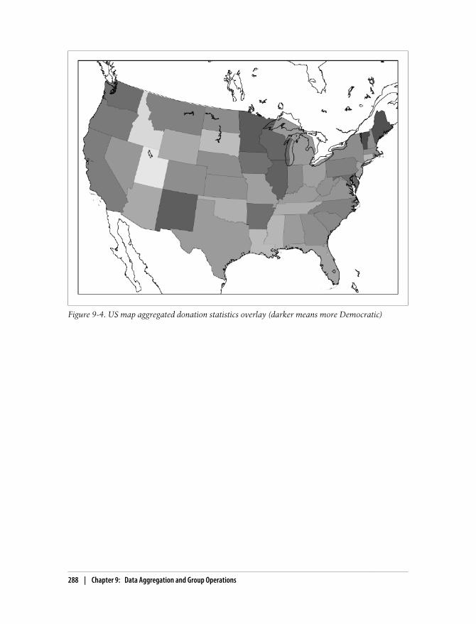
Figure 9-4. US map aggregated donation statistics overlay (darker means more Democratic)
288 | Chapter 9: Data Aggregation and Group Operations

CHAPTER 10
Time Series
Time series data is an important form of structured data in many different fields, suchas finance, economics, ecology, neuroscience, or physics. Anything that is observed ormeasured at many points in time forms a time series. Many time series are fixed fre-quency, which is to say that data points occur at regular intervals according to somerule, such as every 15 seconds, every 5 minutes, or once per month. Time series canalso be irregular without a fixed unit or time or offset between units. How you markand refer to time series data depends on the application and you may have one of thefollowing:
• Timestamps, specific instants in time
• Fixed periods, such as the month January 2007 or the full year 2010
• Intervals of time, indicated by a start and end timestamp. Periods can be thoughtof as special cases of intervals
• Experiment or elapsed time; each timestamp is a measure of time relative to aparticular start time. For example, the diameter of a cookie baking each secondsince being placed in the oven
In this chapter, I am mainly concerned with time series in the first 3 categories, thoughmany of the techniques can be applied to experimental time series where the index maybe an integer or floating point number indicating elapsed time from the start of theexperiment. The simplest and most widely used kind of time series are those indexedby timestamp.
pandas provides a standard set of time series tools and data algorithms. With this, youcan efficiently work with very large time series and easily slice and dice, aggregate, andresample irregular and fixed frequency time series. As you might guess, many of thesetools are especially useful for financial and economics applications, but you could cer-tainly use them to analyze server log data, too.
289

Some of the features and code, in particular period logic, presented inthis chapter were derived from the now defunct scikits.timeseries li-brary.
Date and Time Data Types and ToolsThe Python standard library includes data types for date and time data, as well ascalendar-related functionality. The datetime, time, and calendar modules are the mainplaces to start. The datetime.datetime type, or simply datetime, is widely used:
In [317]: from datetime import datetime
In [318]: now = datetime.now()
In [319]: nowOut[319]: datetime.datetime(2012, 8, 4, 17, 9, 21, 832092)
In [320]: now.year, now.month, now.dayOut[320]: (2012, 8, 4)
datetime stores both the date and time down to the microsecond. datetime.timedelta represents the temporal difference between two datetime objects:
In [321]: delta = datetime(2011, 1, 7) - datetime(2008, 6, 24, 8, 15)
In [322]: deltaOut[322]: datetime.timedelta(926, 56700)
In [323]: delta.days In [324]: delta.secondsOut[323]: 926 Out[324]: 56700
You can add (or subtract) a timedelta or multiple thereof to a datetime object to yielda new shifted object:
In [325]: from datetime import timedelta
In [326]: start = datetime(2011, 1, 7)
In [327]: start + timedelta(12)Out[327]: datetime.datetime(2011, 1, 19, 0, 0)
In [328]: start - 2 * timedelta(12)Out[328]: datetime.datetime(2010, 12, 14, 0, 0)
The data types in the datetime module are summarized in Table 10-1. While this chap-ter is mainly concerned with the data types in pandas and higher level time series ma-nipulation, you will undoubtedly encounter the datetime-based types in many otherplaces in Python the wild.
290 | Chapter 10: Time Series

Table 10-1. Types in datetime module
Type Description
date Store calendar date (year, month, day) using the Gregorian calendar.
time Store time of day as hours, minutes, seconds, and microseconds
datetime Stores both date and time
timedelta Represents the difference between two datetime values (as days, seconds, and micro-seconds)
Converting between string and datetimedatetime objects and pandas Timestamp objects, which I’ll introduce later, can be for-matted as strings using str or the strftime method, passing a format specification:
In [329]: stamp = datetime(2011, 1, 3)
In [330]: str(stamp) In [331]: stamp.strftime('%Y-%m-%d')Out[330]: '2011-01-03 00:00:00' Out[331]: '2011-01-03'
See Table 10-2 for a complete list of the format codes. These same format codes can beused to convert strings to dates using datetime.strptime:
In [332]: value = '2011-01-03'
In [333]: datetime.strptime(value, '%Y-%m-%d')Out[333]: datetime.datetime(2011, 1, 3, 0, 0)
In [334]: datestrs = ['7/6/2011', '8/6/2011']
In [335]: [datetime.strptime(x, '%m/%d/%Y') for x in datestrs]Out[335]: [datetime.datetime(2011, 7, 6, 0, 0), datetime.datetime(2011, 8, 6, 0, 0)]
datetime.strptime is the best way to parse a date with a known format. However, itcan be a bit annoying to have to write a format spec each time, especially for commondate formats. In this case, you can use the parser.parse method in the third party dateutil package:
In [336]: from dateutil.parser import parse
In [337]: parse('2011-01-03')Out[337]: datetime.datetime(2011, 1, 3, 0, 0)
dateutil is capable of parsing almost any human-intelligible date representation:
In [338]: parse('Jan 31, 1997 10:45 PM')Out[338]: datetime.datetime(1997, 1, 31, 22, 45)
In international locales, day appearing before month is very common, so you can passdayfirst=True to indicate this:
In [339]: parse('6/12/2011', dayfirst=True)Out[339]: datetime.datetime(2011, 12, 6, 0, 0)
Date and Time Data Types and Tools | 291
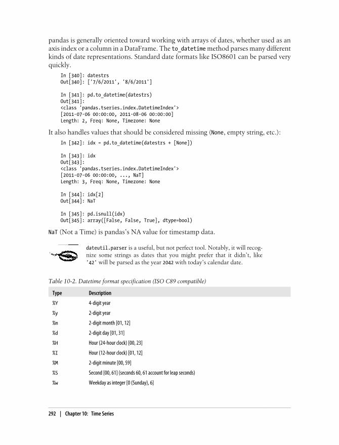
pandas is generally oriented toward working with arrays of dates, whether used as anaxis index or a column in a DataFrame. The to_datetime method parses many differentkinds of date representations. Standard date formats like ISO8601 can be parsed veryquickly.
In [340]: datestrsOut[340]: ['7/6/2011', '8/6/2011']
In [341]: pd.to_datetime(datestrs)Out[341]: <class 'pandas.tseries.index.DatetimeIndex'>[2011-07-06 00:00:00, 2011-08-06 00:00:00]Length: 2, Freq: None, Timezone: None
It also handles values that should be considered missing (None, empty string, etc.):
In [342]: idx = pd.to_datetime(datestrs + [None])
In [343]: idxOut[343]: <class 'pandas.tseries.index.DatetimeIndex'>[2011-07-06 00:00:00, ..., NaT]Length: 3, Freq: None, Timezone: None
In [344]: idx[2]Out[344]: NaT
In [345]: pd.isnull(idx)Out[345]: array([False, False, True], dtype=bool)
NaT (Not a Time) is pandas’s NA value for timestamp data.
dateutil.parser is a useful, but not perfect tool. Notably, it will recog-nize some strings as dates that you might prefer that it didn’t, like'42' will be parsed as the year 2042 with today’s calendar date.
Table 10-2. Datetime format specification (ISO C89 compatible)
Type Description
%Y 4-digit year
%y 2-digit year
%m 2-digit month [01, 12]
%d 2-digit day [01, 31]
%H Hour (24-hour clock) [00, 23]
%I Hour (12-hour clock) [01, 12]
%M 2-digit minute [00, 59]
%S Second [00, 61] (seconds 60, 61 account for leap seconds)
%w Weekday as integer [0 (Sunday), 6]
292 | Chapter 10: Time Series
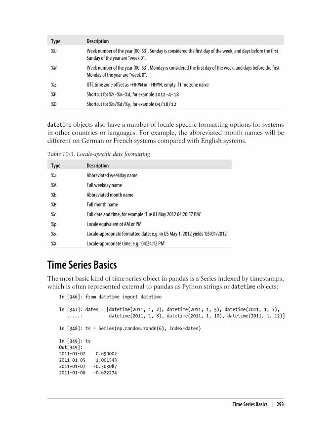
Type Description
%U Week number of the year [00, 53]. Sunday is considered the first day of the week, and days before the firstSunday of the year are “week 0”.
%W Week number of the year [00, 53]. Monday is considered the first day of the week, and days before the firstMonday of the year are “week 0”.
%z UTC time zone offset as +HHMM or -HHMM, empty if time zone naive
%F Shortcut for %Y-%m-%d, for example 2012-4-18
%D Shortcut for %m/%d/%y, for example 04/18/12
datetime objects also have a number of locale-specific formatting options for systemsin other countries or languages. For example, the abbreviated month names will bedifferent on German or French systems compared with English systems.
Table 10-3. Locale-specific date formatting
Type Description
%a Abbreviated weekday name
%A Full weekday name
%b Abbreviated month name
%B Full month name
%c Full date and time, for example ‘Tue 01 May 2012 04:20:57 PM’
%p Locale equivalent of AM or PM
%x Locale-appropriate formatted date; e.g. in US May 1, 2012 yields ’05/01/2012’
%X Locale-appropriate time, e.g. ’04:24:12 PM’
Time Series BasicsThe most basic kind of time series object in pandas is a Series indexed by timestamps,which is often represented external to pandas as Python strings or datetime objects:
In [346]: from datetime import datetime
In [347]: dates = [datetime(2011, 1, 2), datetime(2011, 1, 5), datetime(2011, 1, 7), .....: datetime(2011, 1, 8), datetime(2011, 1, 10), datetime(2011, 1, 12)]
In [348]: ts = Series(np.random.randn(6), index=dates)
In [349]: tsOut[349]: 2011-01-02 0.6900022011-01-05 1.0015432011-01-07 -0.5030872011-01-08 -0.622274
Time Series Basics | 293

2011-01-10 -0.9211692011-01-12 -0.726213
Under the hood, these datetime objects have been put in a DatetimeIndex, and thevariable ts is now of type TimeSeries:
In [350]: type(ts)Out[350]: pandas.core.series.TimeSeries
In [351]: ts.indexOut[351]: <class 'pandas.tseries.index.DatetimeIndex'>[2011-01-02 00:00:00, ..., 2011-01-12 00:00:00]Length: 6, Freq: None, Timezone: None
It’s not necessary to use the TimeSeries constructor explicitly; whencreating a Series with a DatetimeIndex, pandas knows that the object isa time series.
Like other Series, arithmetic operations between differently-indexed time series auto-matically align on the dates:
In [352]: ts + ts[::2]Out[352]: 2011-01-02 1.3800042011-01-05 NaN2011-01-07 -1.0061752011-01-08 NaN2011-01-10 -1.8423372011-01-12 NaN
pandas stores timestamps using NumPy’s datetime64 data type at the nanosecond res-olution:
In [353]: ts.index.dtypeOut[353]: dtype('datetime64[ns]')
Scalar values from a DatetimeIndex are pandas Timestamp objects
In [354]: stamp = ts.index[0]
In [355]: stampOut[355]: <Timestamp: 2011-01-02 00:00:00>
A Timestamp can be substituted anywhere you would use a datetime object. Addition-ally, it can store frequency information (if any) and understands how to do time zoneconversions and other kinds of manipulations. More on both of these things later.
Indexing, Selection, SubsettingTimeSeries is a subclass of Series and thus behaves in the same way with regard toindexing and selecting data based on label:
294 | Chapter 10: Time Series

In [356]: stamp = ts.index[2]
In [357]: ts[stamp]Out[357]: -0.50308739136034464
As a convenience, you can also pass a string that is interpretable as a date:
In [358]: ts['1/10/2011'] In [359]: ts['20110110'] Out[358]: -0.92116860801301081 Out[359]: -0.92116860801301081
For longer time series, a year or only a year and month can be passed to easily selectslices of data:
In [360]: longer_ts = Series(np.random.randn(1000), .....: index=pd.date_range('1/1/2000', periods=1000))
In [361]: longer_tsOut[361]: 2000-01-01 0.2228962000-01-02 0.0513162000-01-03 -1.1577192000-01-04 0.816707...2002-09-23 -0.3958132002-09-24 -0.1807372002-09-25 1.3375082002-09-26 -0.416584Freq: D, Length: 1000
In [362]: longer_ts['2001'] In [363]: longer_ts['2001-05']Out[362]: Out[363]: 2001-01-01 -1.499503 2001-05-01 1.662014 2001-01-02 0.545154 2001-05-02 -1.189203 2001-01-03 0.400823 2001-05-03 0.093597 2001-01-04 -1.946230 2001-05-04 -0.539164 ... ... 2001-12-28 -1.568139 2001-05-28 -0.683066 2001-12-29 -0.900887 2001-05-29 -0.950313 2001-12-30 0.652346 2001-05-30 0.400710 2001-12-31 0.871600 2001-05-31 -0.126072 Freq: D, Length: 365 Freq: D, Length: 31
Slicing with dates works just like with a regular Series:
In [364]: ts[datetime(2011, 1, 7):]Out[364]: 2011-01-07 -0.5030872011-01-08 -0.6222742011-01-10 -0.9211692011-01-12 -0.726213
Because most time series data is ordered chronologically, you can slice with timestampsnot contained in a time series to perform a range query:
In [365]: ts In [366]: ts['1/6/2011':'1/11/2011']Out[365]: Out[366]: 2011-01-02 0.690002 2011-01-07 -0.503087
Time Series Basics | 295

2011-01-05 1.001543 2011-01-08 -0.622274 2011-01-07 -0.503087 2011-01-10 -0.921169 2011-01-08 -0.622274 2011-01-10 -0.921169 2011-01-12 -0.726213
As before you can pass either a string date, datetime, or Timestamp. Remember thatslicing in this manner produces views on the source time series just like slicing NumPyarrays. There is an equivalent instance method truncate which slices a TimeSeries be-tween two dates:
In [367]: ts.truncate(after='1/9/2011')Out[367]: 2011-01-02 0.6900022011-01-05 1.0015432011-01-07 -0.5030872011-01-08 -0.622274
All of the above holds true for DataFrame as well, indexing on its rows:
In [368]: dates = pd.date_range('1/1/2000', periods=100, freq='W-WED')
In [369]: long_df = DataFrame(np.random.randn(100, 4), .....: index=dates, .....: columns=['Colorado', 'Texas', 'New York', 'Ohio'])
In [370]: long_df.ix['5-2001']Out[370]: Colorado Texas New York Ohio2001-05-02 0.943479 -0.349366 0.530412 -0.5087242001-05-09 0.230643 -0.065569 -0.248717 -0.5871362001-05-16 -1.022324 1.060661 0.954768 -0.5118242001-05-23 -1.387680 0.767902 -1.164490 1.5270702001-05-30 0.287542 0.715359 -0.345805 0.470886
Time Series with Duplicate IndicesIn some applications, there may be multiple data observations falling on a particulartimestamp. Here is an example:
In [371]: dates = pd.DatetimeIndex(['1/1/2000', '1/2/2000', '1/2/2000', '1/2/2000', .....: '1/3/2000'])
In [372]: dup_ts = Series(np.arange(5), index=dates)
In [373]: dup_tsOut[373]: 2000-01-01 02000-01-02 12000-01-02 22000-01-02 32000-01-03 4
We can tell that the index is not unique by checking its is_unique property:
296 | Chapter 10: Time Series
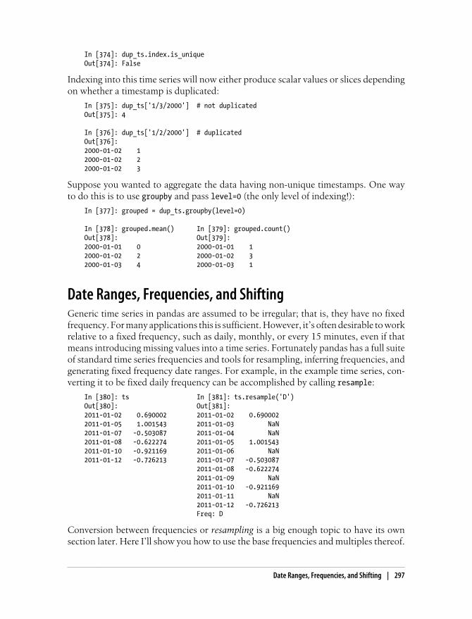
In [374]: dup_ts.index.is_uniqueOut[374]: False
Indexing into this time series will now either produce scalar values or slices dependingon whether a timestamp is duplicated:
In [375]: dup_ts['1/3/2000'] # not duplicatedOut[375]: 4
In [376]: dup_ts['1/2/2000'] # duplicatedOut[376]: 2000-01-02 12000-01-02 22000-01-02 3
Suppose you wanted to aggregate the data having non-unique timestamps. One wayto do this is to use groupby and pass level=0 (the only level of indexing!):
In [377]: grouped = dup_ts.groupby(level=0)
In [378]: grouped.mean() In [379]: grouped.count()Out[378]: Out[379]: 2000-01-01 0 2000-01-01 1 2000-01-02 2 2000-01-02 3 2000-01-03 4 2000-01-03 1
Date Ranges, Frequencies, and ShiftingGeneric time series in pandas are assumed to be irregular; that is, they have no fixedfrequency. For many applications this is sufficient. However, it’s often desirable to workrelative to a fixed frequency, such as daily, monthly, or every 15 minutes, even if thatmeans introducing missing values into a time series. Fortunately pandas has a full suiteof standard time series frequencies and tools for resampling, inferring frequencies, andgenerating fixed frequency date ranges. For example, in the example time series, con-verting it to be fixed daily frequency can be accomplished by calling resample:
In [380]: ts In [381]: ts.resample('D')Out[380]: Out[381]: 2011-01-02 0.690002 2011-01-02 0.690002 2011-01-05 1.001543 2011-01-03 NaN 2011-01-07 -0.503087 2011-01-04 NaN 2011-01-08 -0.622274 2011-01-05 1.001543 2011-01-10 -0.921169 2011-01-06 NaN 2011-01-12 -0.726213 2011-01-07 -0.503087 2011-01-08 -0.622274 2011-01-09 NaN 2011-01-10 -0.921169 2011-01-11 NaN 2011-01-12 -0.726213 Freq: D
Conversion between frequencies or resampling is a big enough topic to have its ownsection later. Here I’ll show you how to use the base frequencies and multiples thereof.
Date Ranges, Frequencies, and Shifting | 297

Generating Date RangesWhile I used it previously without explanation, you may have guessed that pandas.date_range is responsible for generating a DatetimeIndex with an indicated lengthaccording to a particular frequency:
In [382]: index = pd.date_range('4/1/2012', '6/1/2012')
In [383]: indexOut[383]: <class 'pandas.tseries.index.DatetimeIndex'>[2012-04-01 00:00:00, ..., 2012-06-01 00:00:00]Length: 62, Freq: D, Timezone: None
By default, date_range generates daily timestamps. If you pass only a start or end date,you must pass a number of periods to generate:
In [384]: pd.date_range(start='4/1/2012', periods=20)Out[384]: <class 'pandas.tseries.index.DatetimeIndex'>[2012-04-01 00:00:00, ..., 2012-04-20 00:00:00]Length: 20, Freq: D, Timezone: None
In [385]: pd.date_range(end='6/1/2012', periods=20)Out[385]: <class 'pandas.tseries.index.DatetimeIndex'>[2012-05-13 00:00:00, ..., 2012-06-01 00:00:00]Length: 20, Freq: D, Timezone: None
The start and end dates define strict boundaries for the generated date index. For ex-ample, if you wanted a date index containing the last business day of each month, youwould pass the 'BM' frequency (business end of month) and only dates falling on orinside the date interval will be included:
In [386]: pd.date_range('1/1/2000', '12/1/2000', freq='BM')Out[386]: <class 'pandas.tseries.index.DatetimeIndex'>[2000-01-31 00:00:00, ..., 2000-11-30 00:00:00]Length: 11, Freq: BM, Timezone: None
date_range by default preserves the time (if any) of the start or end timestamp:
In [387]: pd.date_range('5/2/2012 12:56:31', periods=5)Out[387]: <class 'pandas.tseries.index.DatetimeIndex'>[2012-05-02 12:56:31, ..., 2012-05-06 12:56:31]Length: 5, Freq: D, Timezone: None
Sometimes you will have start or end dates with time information but want to generatea set of timestamps normalized to midnight as a convention. To do this, there is anormalize option:
In [388]: pd.date_range('5/2/2012 12:56:31', periods=5, normalize=True)Out[388]: <class 'pandas.tseries.index.DatetimeIndex'>
298 | Chapter 10: Time Series

[2012-05-02 00:00:00, ..., 2012-05-06 00:00:00]Length: 5, Freq: D, Timezone: None
Frequencies and Date OffsetsFrequencies in pandas are composed of a base frequency and a multiplier. Base fre-quencies are typically referred to by a string alias, like 'M' for monthly or 'H' for hourly.For each base frequency, there is an object defined generally referred to as a date off-set. For example, hourly frequency can be represented with the Hour class:
In [389]: from pandas.tseries.offsets import Hour, Minute
In [390]: hour = Hour()
In [391]: hourOut[391]: <1 Hour>
You can define a multiple of an offset by passing an integer:
In [392]: four_hours = Hour(4)
In [393]: four_hoursOut[393]: <4 Hours>
In most applications, you would never need to explicitly create one of these objects,instead using a string alias like 'H' or '4H'. Putting an integer before the base frequencycreates a multiple:
In [394]: pd.date_range('1/1/2000', '1/3/2000 23:59', freq='4h')Out[394]: <class 'pandas.tseries.index.DatetimeIndex'>[2000-01-01 00:00:00, ..., 2000-01-03 20:00:00]Length: 18, Freq: 4H, Timezone: None
Many offsets can be combined together by addition:
In [395]: Hour(2) + Minute(30)Out[395]: <150 Minutes>
Similarly, you can pass frequency strings like '2h30min' which will effectively be parsedto the same expression:
In [396]: pd.date_range('1/1/2000', periods=10, freq='1h30min')Out[396]: <class 'pandas.tseries.index.DatetimeIndex'>[2000-01-01 00:00:00, ..., 2000-01-01 13:30:00]Length: 10, Freq: 90T, Timezone: None
Some frequencies describe points in time that are not evenly spaced. For example,'M' (calendar month end) and 'BM' (last business/weekday of month) depend on thenumber of days in a month and, in the latter case, whether the month ends on a weekendor not. For lack of a better term, I call these anchored offsets.
See Table 10-4 for a listing of frequency codes and date offset classes available in pandas.
Date Ranges, Frequencies, and Shifting | 299
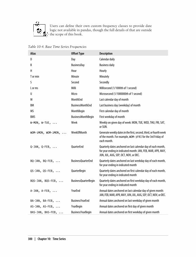
Users can define their own custom frequency classes to provide datelogic not available in pandas, though the full details of that are outsidethe scope of this book.
Table 10-4. Base Time Series Frequencies
Alias Offset Type Description
D Day Calendar daily
B BusinessDay Business daily
H Hour Hourly
T or min Minute Minutely
S Second Secondly
L or ms Milli Millisecond (1/1000th of 1 second)
U Micro Microsecond (1/1000000th of 1 second)
M MonthEnd Last calendar day of month
BM BusinessMonthEnd Last business day (weekday) of month
MS MonthBegin First calendar day of month
BMS BusinessMonthBegin First weekday of month
W-MON, W-TUE, ... Week Weekly on given day of week: MON, TUE, WED, THU, FRI, SAT,or SUN.
WOM-1MON, WOM-2MON, ... WeekOfMonth Generate weekly dates in the first, second, third, or fourth weekof the month. For example, WOM-3FRI for the 3rd Friday ofeach month.
Q-JAN, Q-FEB, ... QuarterEnd Quarterly dates anchored on last calendar day of each month,for year ending in indicated month: JAN, FEB, MAR, APR, MAY,JUN, JUL, AUG, SEP, OCT, NOV, or DEC.
BQ-JAN, BQ-FEB, ... BusinessQuarterEnd Quarterly dates anchored on last weekday day of each month,for year ending in indicated month
QS-JAN, QS-FEB, ... QuarterBegin Quarterly dates anchored on first calendar day of each month,for year ending in indicated month
BQS-JAN, BQS-FEB, ... BusinessQuarterBegin Quarterly dates anchored on first weekday day of each month,for year ending in indicated month
A-JAN, A-FEB, ... YearEnd Annual dates anchored on last calendar day of given month:JAN, FEB, MAR, APR, MAY, JUN, JUL, AUG, SEP, OCT, NOV, or DEC.
BA-JAN, BA-FEB, ... BusinessYearEnd Annual dates anchored on last weekday of given month
AS-JAN, AS-FEB, ... YearBegin Annual dates anchored on first day of given month
BAS-JAN, BAS-FEB, ... BusinessYearBegin Annual dates anchored on first weekday of given month
300 | Chapter 10: Time Series

Week of month dates
One useful frequency class is “week of month”, starting with WOM. This enables you toget dates like the third Friday of each month:
In [397]: rng = pd.date_range('1/1/2012', '9/1/2012', freq='WOM-3FRI')
In [398]: list(rng)Out[398]: [<Timestamp: 2012-01-20 00:00:00>, <Timestamp: 2012-02-17 00:00:00>, <Timestamp: 2012-03-16 00:00:00>, <Timestamp: 2012-04-20 00:00:00>, <Timestamp: 2012-05-18 00:00:00>, <Timestamp: 2012-06-15 00:00:00>, <Timestamp: 2012-07-20 00:00:00>, <Timestamp: 2012-08-17 00:00:00>]
Traders of US equity options will recognize these dates as the standard dates of monthlyexpiry.
Shifting (Leading and Lagging) Data“Shifting” refers to moving data backward and forward through time. Both Series andDataFrame have a shift method for doing naive shifts forward or backward, leavingthe index unmodified:
In [399]: ts = Series(np.random.randn(4), .....: index=pd.date_range('1/1/2000', periods=4, freq='M'))
In [400]: ts In [401]: ts.shift(2) In [402]: ts.shift(-2)Out[400]: Out[401]: Out[402]: 2000-01-31 0.575283 2000-01-31 NaN 2000-01-31 1.8145822000-02-29 0.304205 2000-02-29 NaN 2000-02-29 1.6348582000-03-31 1.814582 2000-03-31 0.575283 2000-03-31 NaN2000-04-30 1.634858 2000-04-30 0.304205 2000-04-30 NaNFreq: M Freq: M Freq: M
A common use of shift is computing percent changes in a time series or multiple timeseries as DataFrame columns. This is expressed as
ts / ts.shift(1) - 1
Because naive shifts leave the index unmodified, some data is discarded. Thus if thefrequency is known, it can be passed to shift to advance the timestamps instead ofsimply the data:
In [403]: ts.shift(2, freq='M')Out[403]: 2000-03-31 0.5752832000-04-30 0.3042052000-05-31 1.8145822000-06-30 1.634858Freq: M
Date Ranges, Frequencies, and Shifting | 301

Other frequencies can be passed, too, giving you a lot of flexibility in how to lead andlag the data:
In [404]: ts.shift(3, freq='D') In [405]: ts.shift(1, freq='3D')Out[404]: Out[405]: 2000-02-03 0.575283 2000-02-03 0.575283 2000-03-03 0.304205 2000-03-03 0.304205 2000-04-03 1.814582 2000-04-03 1.814582 2000-05-03 1.634858 2000-05-03 1.634858 In [406]: ts.shift(1, freq='90T')Out[406]: 2000-01-31 01:30:00 0.5752832000-02-29 01:30:00 0.3042052000-03-31 01:30:00 1.8145822000-04-30 01:30:00 1.634858
Shifting dates with offsets
The pandas date offsets can also be used with datetime or Timestamp objects:
In [407]: from pandas.tseries.offsets import Day, MonthEnd
In [408]: now = datetime(2011, 11, 17)
In [409]: now + 3 * Day()Out[409]: datetime.datetime(2011, 11, 20, 0, 0)
If you add an anchored offset like MonthEnd, the first increment will roll forward a dateto the next date according to the frequency rule:
In [410]: now + MonthEnd()Out[410]: datetime.datetime(2011, 11, 30, 0, 0)
In [411]: now + MonthEnd(2)Out[411]: datetime.datetime(2011, 12, 31, 0, 0)
Anchored offsets can explicitly “roll” dates forward or backward using their rollforward and rollback methods, respectively:
In [412]: offset = MonthEnd()
In [413]: offset.rollforward(now)Out[413]: datetime.datetime(2011, 11, 30, 0, 0)
In [414]: offset.rollback(now)Out[414]: datetime.datetime(2011, 10, 31, 0, 0)
A clever use of date offsets is to use these methods with groupby:
In [415]: ts = Series(np.random.randn(20), .....: index=pd.date_range('1/15/2000', periods=20, freq='4d'))
In [416]: ts.groupby(offset.rollforward).mean()Out[416]: 2000-01-31 -0.448874
302 | Chapter 10: Time Series

2000-02-29 -0.6836632000-03-31 0.251920
Of course, an easier and faster way to do this is using resample (much more on this later):
In [417]: ts.resample('M', how='mean')Out[417]: 2000-01-31 -0.4488742000-02-29 -0.6836632000-03-31 0.251920Freq: M
Time Zone HandlingWorking with time zones is generally considered one of the most unpleasant parts oftime series manipulation. In particular, daylight savings time (DST) transitions are acommon source of complication. As such, many time series users choose to work withtime series in coordinated universal time or UTC, which is the successor to GreenwichMean Time and is the current international standard. Time zones are expressed asoffsets from UTC; for example, New York is four hours behind UTC during daylightsavings time and 5 hours the rest of the year.
In Python, time zone information comes from the 3rd party pytz library, which exposesthe Olson database, a compilation of world time zone information. This is especiallyimportant for historical data because the DST transition dates (and even UTC offsets)have been changed numerous times depending on the whims of local governments. Inthe United States,the DST transition times have been changed many times since 1900!
For detailed information about pytz library, you’ll need to look at that library’s docu-mentation. As far as this book is concerned, pandas wraps pytz’s functionality so youcan ignore its API outside of the time zone names. Time zone names can be foundinteractively and in the docs:
In [418]: import pytz
In [419]: pytz.common_timezones[-5:]Out[419]: ['US/Eastern', 'US/Hawaii', 'US/Mountain', 'US/Pacific', 'UTC']
To get a time zone object from pytz, use pytz.timezone:
In [420]: tz = pytz.timezone('US/Eastern')
In [421]: tzOut[421]: <DstTzInfo 'US/Eastern' EST-1 day, 19:00:00 STD>
Methods in pandas will accept either time zone names or these objects. I recommendjust using the names.
Time Zone Handling | 303

Localization and ConversionBy default, time series in pandas are time zone naive. Consider the following time series:
rng = pd.date_range('3/9/2012 9:30', periods=6, freq='D')ts = Series(np.random.randn(len(rng)), index=rng)
The index’s tz field is None:
In [423]: print(ts.index.tz)None
Date ranges can be generated with a time zone set:
In [424]: pd.date_range('3/9/2012 9:30', periods=10, freq='D', tz='UTC')Out[424]: <class 'pandas.tseries.index.DatetimeIndex'>[2012-03-09 09:30:00, ..., 2012-03-18 09:30:00]Length: 10, Freq: D, Timezone: UTC
Conversion from naive to localized is handled by the tz_localize method:
In [425]: ts_utc = ts.tz_localize('UTC')
In [426]: ts_utcOut[426]: 2012-03-09 09:30:00+00:00 0.4146152012-03-10 09:30:00+00:00 0.4271852012-03-11 09:30:00+00:00 1.1725572012-03-12 09:30:00+00:00 -0.3515722012-03-13 09:30:00+00:00 1.4545932012-03-14 09:30:00+00:00 2.043319Freq: D
In [427]: ts_utc.indexOut[427]: <class 'pandas.tseries.index.DatetimeIndex'>[2012-03-09 09:30:00, ..., 2012-03-14 09:30:00]Length: 6, Freq: D, Timezone: UTC
Once a time series has been localized to a particular time zone, it can be converted toanother time zone using tz_convert:
In [428]: ts_utc.tz_convert('US/Eastern')Out[428]: 2012-03-09 04:30:00-05:00 0.4146152012-03-10 04:30:00-05:00 0.4271852012-03-11 05:30:00-04:00 1.1725572012-03-12 05:30:00-04:00 -0.3515722012-03-13 05:30:00-04:00 1.4545932012-03-14 05:30:00-04:00 2.043319Freq: D
In the case of the above time series, which straddles a DST transition in the US/Easterntime zone, we could localize to EST and convert to, say, UTC or Berlin time:
In [429]: ts_eastern = ts.tz_localize('US/Eastern')
304 | Chapter 10: Time Series

In [430]: ts_eastern.tz_convert('UTC')Out[430]: 2012-03-09 14:30:00+00:00 0.4146152012-03-10 14:30:00+00:00 0.4271852012-03-11 13:30:00+00:00 1.1725572012-03-12 13:30:00+00:00 -0.3515722012-03-13 13:30:00+00:00 1.4545932012-03-14 13:30:00+00:00 2.043319Freq: D
In [431]: ts_eastern.tz_convert('Europe/Berlin')Out[431]: 2012-03-09 15:30:00+01:00 0.4146152012-03-10 15:30:00+01:00 0.4271852012-03-11 14:30:00+01:00 1.1725572012-03-12 14:30:00+01:00 -0.3515722012-03-13 14:30:00+01:00 1.4545932012-03-14 14:30:00+01:00 2.043319Freq: D
tz_localize and tz_convert are also instance methods on DatetimeIndex:
In [432]: ts.index.tz_localize('Asia/Shanghai')Out[432]: <class 'pandas.tseries.index.DatetimeIndex'>[2012-03-09 09:30:00, ..., 2012-03-14 09:30:00]Length: 6, Freq: D, Timezone: Asia/Shanghai
Localizing naive timestamps also checks for ambiguous or non-existenttimes around daylight savings time transitions.
Operations with Time Zone−aware Timestamp ObjectsSimilar to time series and date ranges, individual Timestamp objects similarly can belocalized from naive to time zone-aware and converted from one time zone to another:
In [433]: stamp = pd.Timestamp('2011-03-12 04:00')
In [434]: stamp_utc = stamp.tz_localize('utc')
In [435]: stamp_utc.tz_convert('US/Eastern')Out[435]: <Timestamp: 2011-03-11 23:00:00-0500 EST, tz=US/Eastern>
You can also pass a time zone when creating the Timestamp:
In [436]: stamp_moscow = pd.Timestamp('2011-03-12 04:00', tz='Europe/Moscow')
In [437]: stamp_moscowOut[437]: <Timestamp: 2011-03-12 04:00:00+0300 MSK, tz=Europe/Moscow>
Time zone-aware Timestamp objects internally store a UTC timestamp value as nano-seconds since the UNIX epoch (January 1, 1970); this UTC value is invariant betweentime zone conversions:
Time Zone Handling | 305

In [438]: stamp_utc.valueOut[438]: 1299902400000000000
In [439]: stamp_utc.tz_convert('US/Eastern').valueOut[439]: 1299902400000000000
When performing time arithmetic using pandas’s DateOffset objects, daylight savingstime transitions are respected where possible:
# 30 minutes before DST transitionIn [440]: from pandas.tseries.offsets import Hour
In [441]: stamp = pd.Timestamp('2012-03-12 01:30', tz='US/Eastern')
In [442]: stampOut[442]: <Timestamp: 2012-03-12 01:30:00-0400 EDT, tz=US/Eastern>
In [443]: stamp + Hour()Out[443]: <Timestamp: 2012-03-12 02:30:00-0400 EDT, tz=US/Eastern>
# 90 minutes before DST transitionIn [444]: stamp = pd.Timestamp('2012-11-04 00:30', tz='US/Eastern')
In [445]: stampOut[445]: <Timestamp: 2012-11-04 00:30:00-0400 EDT, tz=US/Eastern>
In [446]: stamp + 2 * Hour()Out[446]: <Timestamp: 2012-11-04 01:30:00-0500 EST, tz=US/Eastern>
Operations between Different Time ZonesIf two time series with different time zones are combined, the result will be UTC. Sincethe timestamps are stored under the hood in UTC, this is a straightforward operationand requires no conversion to happen:
In [447]: rng = pd.date_range('3/7/2012 9:30', periods=10, freq='B')
In [448]: ts = Series(np.random.randn(len(rng)), index=rng)
In [449]: tsOut[449]: 2012-03-07 09:30:00 -1.7493092012-03-08 09:30:00 -0.3872352012-03-09 09:30:00 -0.2080742012-03-12 09:30:00 -1.2219572012-03-13 09:30:00 -0.0674602012-03-14 09:30:00 0.2290052012-03-15 09:30:00 -0.5762342012-03-16 09:30:00 0.8168952012-03-19 09:30:00 -0.7721922012-03-20 09:30:00 -1.333576Freq: B
In [450]: ts1 = ts[:7].tz_localize('Europe/London')
306 | Chapter 10: Time Series

In [451]: ts2 = ts1[2:].tz_convert('Europe/Moscow')
In [452]: result = ts1 + ts2
In [453]: result.indexOut[453]: <class 'pandas.tseries.index.DatetimeIndex'>[2012-03-07 09:30:00, ..., 2012-03-15 09:30:00]Length: 7, Freq: B, Timezone: UTC
Periods and Period ArithmeticPeriods represent time spans, like days, months, quarters, or years. The Period classrepresents this data type, requiring a string or integer and a frequency from the abovetable:
In [454]: p = pd.Period(2007, freq='A-DEC')
In [455]: pOut[455]: Period('2007', 'A-DEC')
In this case, the Period object represents the full timespan from January 1, 2007 toDecember 31, 2007, inclusive. Conveniently, adding and subtracting integers from pe-riods has the effect of shifting by their frequency:
In [456]: p + 5 In [457]: p - 2 Out[456]: Period('2012', 'A-DEC') Out[457]: Period('2005', 'A-DEC')
If two periods have the same frequency, their difference is the number of units betweenthem:
In [458]: pd.Period('2014', freq='A-DEC') - pOut[458]: 7
Regular ranges of periods can be constructed using the period_range function:
In [459]: rng = pd.period_range('1/1/2000', '6/30/2000', freq='M')
In [460]: rngOut[460]: <class 'pandas.tseries.period.PeriodIndex'>freq: M[2000-01, ..., 2000-06]length: 6
The PeriodIndex class stores a sequence of periods and can serve as an axis index inany pandas data structure:
In [461]: Series(np.random.randn(6), index=rng)Out[461]: 2000-01 -0.3091192000-02 0.0285582000-03 1.1296052000-04 -0.3741732000-05 -0.011401
Periods and Period Arithmetic | 307

2000-06 0.272924Freq: M
If you have an array of strings, you can also appeal to the PeriodIndex class itself:
In [462]: values = ['2001Q3', '2002Q2', '2003Q1']
In [463]: index = pd.PeriodIndex(values, freq='Q-DEC')
In [464]: indexOut[464]: <class 'pandas.tseries.period.PeriodIndex'>freq: Q-DEC[2001Q3, ..., 2003Q1]length: 3
Period Frequency ConversionPeriods and PeriodIndex objects can be converted to another frequency using their asfreq method. As an example, suppose we had an annual period and wanted to convertit into a monthly period either at the start or end of the year. This is fairly straightfor-ward:
In [465]: p = pd.Period('2007', freq='A-DEC')
In [466]: p.asfreq('M', how='start') In [467]: p.asfreq('M', how='end')Out[466]: Period('2007-01', 'M') Out[467]: Period('2007-12', 'M')
You can think of Period('2007', 'A-DEC') as being a cursor pointing to a span of time,subdivided by monthly periods. See Figure 10-1 for an illustration of this. For a fiscalyear ending on a month other than December, the monthly subperiods belonging aredifferent:
In [468]: p = pd.Period('2007', freq='A-JUN')
In [469]: p.asfreq('M', 'start') In [470]: p.asfreq('M', 'end') Out[469]: Period('2006-07', 'M') Out[470]: Period('2007-07', 'M')
When converting from high to low frequency, the superperiod will be determined de-pending on where the subperiod “belongs”. For example, in A-JUN frequency, the monthAug-2007 is actually part of the 2008 period:
In [471]: p = pd.Period('2007-08', 'M')
In [472]: p.asfreq('A-JUN')Out[472]: Period('2008', 'A-JUN')
Whole PeriodIndex objects or TimeSeries can be similarly converted with the samesemantics:
In [473]: rng = pd.period_range('2006', '2009', freq='A-DEC')
In [474]: ts = Series(np.random.randn(len(rng)), index=rng)
In [475]: ts
308 | Chapter 10: Time Series

Out[475]: 2006 -0.6015442007 0.5742652008 -0.1941152009 0.202225Freq: A-DEC
In [476]: ts.asfreq('M', how='start') In [477]: ts.asfreq('B', how='end')Out[476]: Out[477]: 2006-01 -0.601544 2006-12-29 -0.601544 2007-01 0.574265 2007-12-31 0.574265 2008-01 -0.194115 2008-12-31 -0.194115 2009-01 0.202225 2009-12-31 0.202225 Freq: M Freq: B
Figure 10-1. Period frequency conversion illustration
Quarterly Period FrequenciesQuarterly data is standard in accounting, finance, and other fields. Much quarterly datais reported relative to a fiscal year end, typically the last calendar or business day of oneof the 12 months of the year. As such, the period 2012Q4 has a different meaning de-pending on fiscal year end. pandas supports all 12 possible quarterly frequencies as Q-JAN through Q-DEC:
In [478]: p = pd.Period('2012Q4', freq='Q-JAN')
In [479]: pOut[479]: Period('2012Q4', 'Q-JAN')
In the case of fiscal year ending in January, 2012Q4 runs from November through Jan-uary, which you can check by converting to daily frequency. See Figure 10-2 for anillustration:
In [480]: p.asfreq('D', 'start') In [481]: p.asfreq('D', 'end') Out[480]: Period('2011-11-01', 'D') Out[481]: Period('2012-01-31', 'D')
Periods and Period Arithmetic | 309
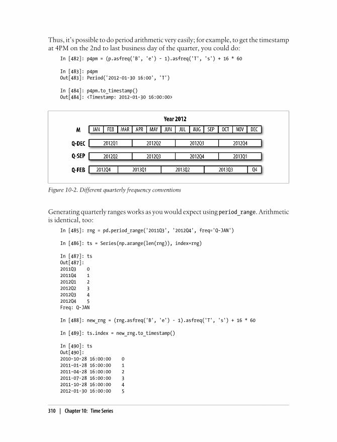
Thus, it’s possible to do period arithmetic very easily; for example, to get the timestampat 4PM on the 2nd to last business day of the quarter, you could do:
In [482]: p4pm = (p.asfreq('B', 'e') - 1).asfreq('T', 's') + 16 * 60
In [483]: p4pmOut[483]: Period('2012-01-30 16:00', 'T')
In [484]: p4pm.to_timestamp()Out[484]: <Timestamp: 2012-01-30 16:00:00>
Figure 10-2. Different quarterly frequency conventions
Generating quarterly ranges works as you would expect using period_range. Arithmeticis identical, too:
In [485]: rng = pd.period_range('2011Q3', '2012Q4', freq='Q-JAN')
In [486]: ts = Series(np.arange(len(rng)), index=rng)
In [487]: tsOut[487]: 2011Q3 02011Q4 12012Q1 22012Q2 32012Q3 42012Q4 5Freq: Q-JAN
In [488]: new_rng = (rng.asfreq('B', 'e') - 1).asfreq('T', 's') + 16 * 60
In [489]: ts.index = new_rng.to_timestamp()
In [490]: tsOut[490]: 2010-10-28 16:00:00 02011-01-28 16:00:00 12011-04-28 16:00:00 22011-07-28 16:00:00 32011-10-28 16:00:00 42012-01-30 16:00:00 5
310 | Chapter 10: Time Series

Converting Timestamps to Periods (and Back)Series and DataFrame objects indexed by timestamps can be converted to periods usingthe to_period method:
In [491]: rng = pd.date_range('1/1/2000', periods=3, freq='M')
In [492]: ts = Series(randn(3), index=rng)
In [493]: pts = ts.to_period()
In [494]: ts In [495]: pts Out[494]: Out[495]: 2000-01-31 -0.505124 2000-01 -0.5051242000-02-29 2.954439 2000-02 2.9544392000-03-31 -2.630247 2000-03 -2.630247Freq: M Freq: M
Since periods always refer to non-overlapping timespans, a timestamp can only belongto a single period for a given frequency. While the frequency of the new PeriodIndex isinferred from the timestamps by default, you can specify any frequency you want. Thereis also no problem with having duplicate periods in the result:
In [496]: rng = pd.date_range('1/29/2000', periods=6, freq='D')
In [497]: ts2 = Series(randn(6), index=rng)
In [498]: ts2.to_period('M')Out[498]: 2000-01 -0.3524532000-01 -0.4778082000-01 0.1615942000-02 1.6868332000-02 0.8219652000-02 -0.667406Freq: M
To convert back to timestamps, use to_timestamp:
In [499]: pts = ts.to_period()
In [500]: ptsOut[500]: 2000-01 -0.5051242000-02 2.9544392000-03 -2.630247Freq: M
In [501]: pts.to_timestamp(how='end')Out[501]: 2000-01-31 -0.5051242000-02-29 2.9544392000-03-31 -2.630247Freq: M
Periods and Period Arithmetic | 311

Creating a PeriodIndex from ArraysFixed frequency data sets are sometimes stored with timespan information spreadacross multiple columns. For example, in this macroeconomic data set, the year andquarter are in different columns:
In [502]: data = pd.read_csv('ch08/macrodata.csv')
In [503]: data.year In [504]: data.quarter Out[503]: Out[504]: 0 1959 0 1 1 1959 1 2 2 1959 2 3 3 1959 3 4 ... ... 199 2008 199 4 200 2009 200 1 201 2009 201 2 202 2009 202 3 Name: year, Length: 203 Name: quarter, Length: 203
By passing these arrays to PeriodIndex with a frequency, they can be combined to forman index for the DataFrame:
In [505]: index = pd.PeriodIndex(year=data.year, quarter=data.quarter, freq='Q-DEC')
In [506]: indexOut[506]: <class 'pandas.tseries.period.PeriodIndex'>freq: Q-DEC[1959Q1, ..., 2009Q3]length: 203
In [507]: data.index = index
In [508]: data.inflOut[508]: 1959Q1 0.001959Q2 2.341959Q3 2.741959Q4 0.27...2008Q4 -8.792009Q1 0.942009Q2 3.372009Q3 3.56Freq: Q-DEC, Name: infl, Length: 203
Resampling and Frequency ConversionResampling refers to the process of converting a time series from one frequency toanother. Aggregating higher frequency data to lower frequency is called downsam-pling, while converting lower frequency to higher frequency is called upsampling. Not
312 | Chapter 10: Time Series
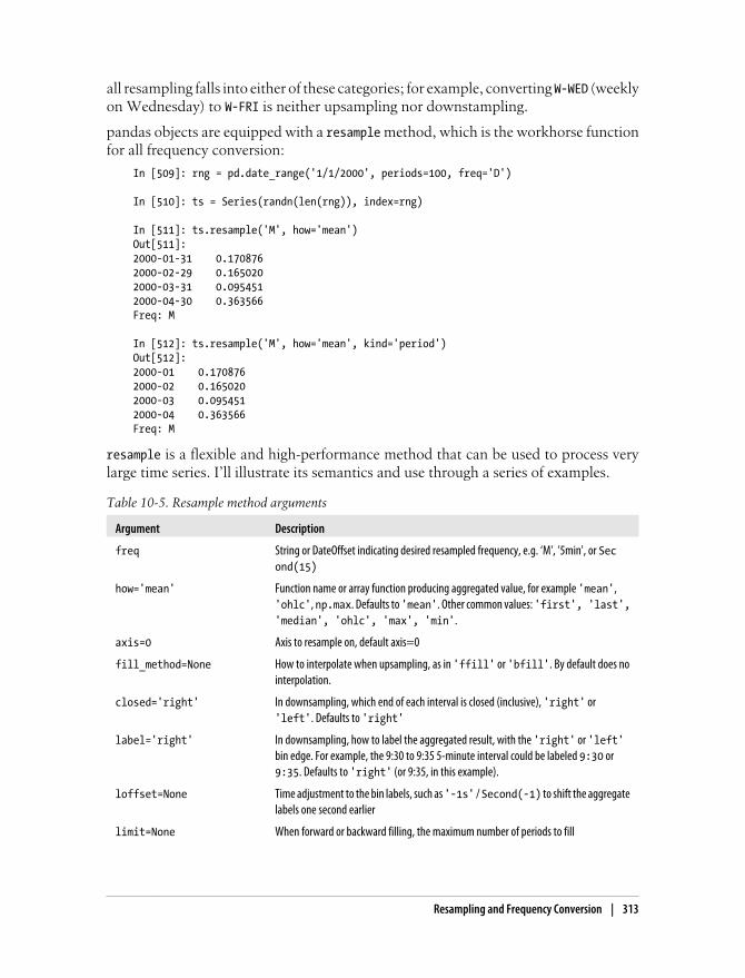
all resampling falls into either of these categories; for example, converting W-WED (weeklyon Wednesday) to W-FRI is neither upsampling nor downstampling.
pandas objects are equipped with a resample method, which is the workhorse functionfor all frequency conversion:
In [509]: rng = pd.date_range('1/1/2000', periods=100, freq='D')
In [510]: ts = Series(randn(len(rng)), index=rng)
In [511]: ts.resample('M', how='mean')Out[511]: 2000-01-31 0.1708762000-02-29 0.1650202000-03-31 0.0954512000-04-30 0.363566Freq: M
In [512]: ts.resample('M', how='mean', kind='period')Out[512]: 2000-01 0.1708762000-02 0.1650202000-03 0.0954512000-04 0.363566Freq: M
resample is a flexible and high-performance method that can be used to process verylarge time series. I’ll illustrate its semantics and use through a series of examples.
Table 10-5. Resample method arguments
Argument Description
freq String or DateOffset indicating desired resampled frequency, e.g. ‘M', ’5min', or Second(15)
how='mean' Function name or array function producing aggregated value, for example 'mean','ohlc', np.max. Defaults to 'mean'. Other common values: 'first', 'last','median', 'ohlc', 'max', 'min'.
axis=0 Axis to resample on, default axis=0
fill_method=None How to interpolate when upsampling, as in 'ffill' or 'bfill'. By default does nointerpolation.
closed='right' In downsampling, which end of each interval is closed (inclusive), 'right' or'left'. Defaults to 'right'
label='right' In downsampling, how to label the aggregated result, with the 'right' or 'left'bin edge. For example, the 9:30 to 9:35 5-minute interval could be labeled 9:30 or9:35. Defaults to 'right' (or 9:35, in this example).
loffset=None Time adjustment to the bin labels, such as '-1s' / Second(-1) to shift the aggregatelabels one second earlier
limit=None When forward or backward filling, the maximum number of periods to fill
Resampling and Frequency Conversion | 313
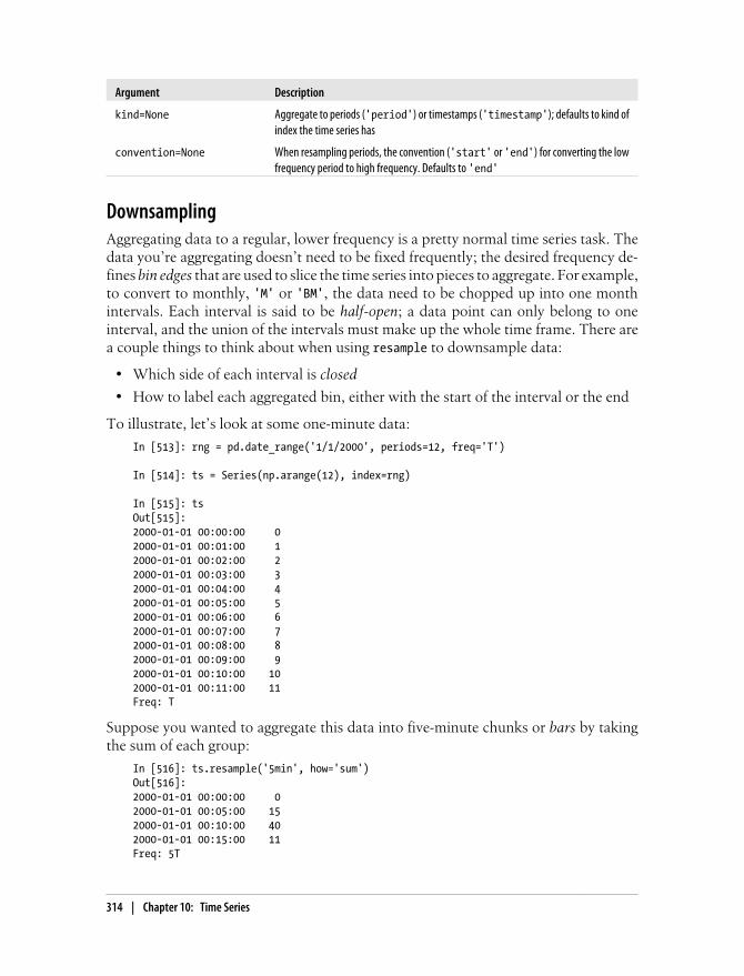
Argument Description
kind=None Aggregate to periods ('period') or timestamps ('timestamp'); defaults to kind ofindex the time series has
convention=None When resampling periods, the convention ('start' or 'end') for converting the lowfrequency period to high frequency. Defaults to 'end'
DownsamplingAggregating data to a regular, lower frequency is a pretty normal time series task. Thedata you’re aggregating doesn’t need to be fixed frequently; the desired frequency de-fines bin edges that are used to slice the time series into pieces to aggregate. For example,to convert to monthly, 'M' or 'BM', the data need to be chopped up into one monthintervals. Each interval is said to be half-open; a data point can only belong to oneinterval, and the union of the intervals must make up the whole time frame. There area couple things to think about when using resample to downsample data:
• Which side of each interval is closed
• How to label each aggregated bin, either with the start of the interval or the end
To illustrate, let’s look at some one-minute data:
In [513]: rng = pd.date_range('1/1/2000', periods=12, freq='T')
In [514]: ts = Series(np.arange(12), index=rng)
In [515]: tsOut[515]: 2000-01-01 00:00:00 02000-01-01 00:01:00 12000-01-01 00:02:00 22000-01-01 00:03:00 32000-01-01 00:04:00 42000-01-01 00:05:00 52000-01-01 00:06:00 62000-01-01 00:07:00 72000-01-01 00:08:00 82000-01-01 00:09:00 92000-01-01 00:10:00 102000-01-01 00:11:00 11Freq: T
Suppose you wanted to aggregate this data into five-minute chunks or bars by takingthe sum of each group:
In [516]: ts.resample('5min', how='sum')Out[516]: 2000-01-01 00:00:00 02000-01-01 00:05:00 152000-01-01 00:10:00 402000-01-01 00:15:00 11Freq: 5T
314 | Chapter 10: Time Series

The frequency you pass defines bin edges in five-minute increments. By default, theright bin edge is inclusive, so the 00:05 value is included in the 00:00 to 00:05 inter-val.1 Passing closed='left' changes the interval to be closed on the left:
In [517]: ts.resample('5min', how='sum', closed='left')Out[517]: 2000-01-01 00:05:00 102000-01-01 00:10:00 352000-01-01 00:15:00 21Freq: 5T
As you can see, the resulting time series is labeled by the timestamps from the right sideof each bin. By passing label='left' you can label them with the left bin edge:
In [518]: ts.resample('5min', how='sum', closed='left', label='left')Out[518]: 2000-01-01 00:00:00 102000-01-01 00:05:00 352000-01-01 00:10:00 21Freq: 5T
See Figure 10-3 for an illustration of minutely data being resampled to five-minute.
Figure 10-3. 5-minute resampling illustration of closed, label conventions
Lastly, you might want to shift the result index by some amount, say subtracting onesecond from the right edge to make it more clear which interval the timestamp refersto. To do this, pass a string or date offset to loffset:
In [519]: ts.resample('5min', how='sum', loffset='-1s')Out[519]: 1999-12-31 23:59:59 02000-01-01 00:04:59 152000-01-01 00:09:59 402000-01-01 00:14:59 11Freq: 5T
1. The choice of closed='right', label='right' as the default might seem a bit odd to some users. Inpractice the choice is somewhat arbitrary; for some target frequencies, closed='left' is preferable, whilefor others closed='right' makes more sense. The important thing is that you keep in mind exactly howyou are segmenting the data.
Resampling and Frequency Conversion | 315
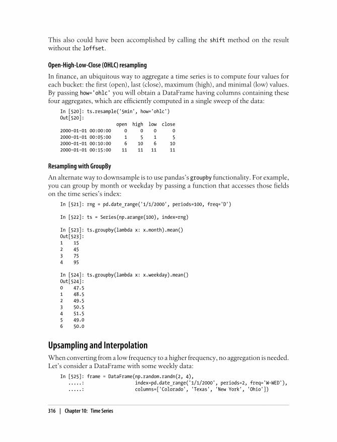
This also could have been accomplished by calling the shift method on the resultwithout the loffset.
Open-High-Low-Close (OHLC) resampling
In finance, an ubiquitous way to aggregate a time series is to compute four values foreach bucket: the first (open), last (close), maximum (high), and minimal (low) values.By passing how='ohlc' you will obtain a DataFrame having columns containing thesefour aggregates, which are efficiently computed in a single sweep of the data:
In [520]: ts.resample('5min', how='ohlc')Out[520]: open high low close2000-01-01 00:00:00 0 0 0 02000-01-01 00:05:00 1 5 1 52000-01-01 00:10:00 6 10 6 102000-01-01 00:15:00 11 11 11 11
Resampling with GroupBy
An alternate way to downsample is to use pandas’s groupby functionality. For example,you can group by month or weekday by passing a function that accesses those fieldson the time series’s index:
In [521]: rng = pd.date_range('1/1/2000', periods=100, freq='D')
In [522]: ts = Series(np.arange(100), index=rng)
In [523]: ts.groupby(lambda x: x.month).mean()Out[523]: 1 152 453 754 95
In [524]: ts.groupby(lambda x: x.weekday).mean()Out[524]: 0 47.51 48.52 49.53 50.54 51.55 49.06 50.0
Upsampling and InterpolationWhen converting from a low frequency to a higher frequency, no aggregation is needed.Let’s consider a DataFrame with some weekly data:
In [525]: frame = DataFrame(np.random.randn(2, 4), .....: index=pd.date_range('1/1/2000', periods=2, freq='W-WED'), .....: columns=['Colorado', 'Texas', 'New York', 'Ohio'])
316 | Chapter 10: Time Series

In [526]: frame[:5]Out[526]: Colorado Texas New York Ohio2000-01-05 -0.609657 -0.268837 0.195592 0.859792000-01-12 -0.263206 1.141350 -0.101937 -0.07666
When resampling this to daily frequency, by default missing values are introduced:
In [527]: df_daily = frame.resample('D')
In [528]: df_dailyOut[528]: Colorado Texas New York Ohio2000-01-05 -0.609657 -0.268837 0.195592 0.859792000-01-06 NaN NaN NaN NaN2000-01-07 NaN NaN NaN NaN2000-01-08 NaN NaN NaN NaN2000-01-09 NaN NaN NaN NaN2000-01-10 NaN NaN NaN NaN2000-01-11 NaN NaN NaN NaN2000-01-12 -0.263206 1.141350 -0.101937 -0.07666
Suppose you wanted to fill forward each weekly value on the non-Wednesdays. Thesame filling or interpolation methods available in the fillna and reindex methods areavailable for resampling:
In [529]: frame.resample('D', fill_method='ffill')Out[529]: Colorado Texas New York Ohio2000-01-05 -0.609657 -0.268837 0.195592 0.859792000-01-06 -0.609657 -0.268837 0.195592 0.859792000-01-07 -0.609657 -0.268837 0.195592 0.859792000-01-08 -0.609657 -0.268837 0.195592 0.859792000-01-09 -0.609657 -0.268837 0.195592 0.859792000-01-10 -0.609657 -0.268837 0.195592 0.859792000-01-11 -0.609657 -0.268837 0.195592 0.859792000-01-12 -0.263206 1.141350 -0.101937 -0.07666
You can similarly choose to only fill a certain number of periods forward to limit howfar to continue using an observed value:
In [530]: frame.resample('D', fill_method='ffill', limit=2)Out[530]: Colorado Texas New York Ohio2000-01-05 -0.609657 -0.268837 0.195592 0.859792000-01-06 -0.609657 -0.268837 0.195592 0.859792000-01-07 -0.609657 -0.268837 0.195592 0.859792000-01-08 NaN NaN NaN NaN2000-01-09 NaN NaN NaN NaN2000-01-10 NaN NaN NaN NaN2000-01-11 NaN NaN NaN NaN2000-01-12 -0.263206 1.141350 -0.101937 -0.07666
Notably, the new date index need not overlap with the old one at all:
Resampling and Frequency Conversion | 317
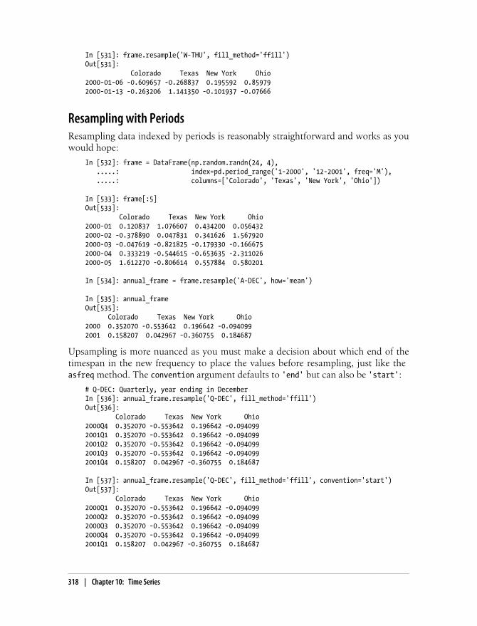
In [531]: frame.resample('W-THU', fill_method='ffill')Out[531]: Colorado Texas New York Ohio2000-01-06 -0.609657 -0.268837 0.195592 0.859792000-01-13 -0.263206 1.141350 -0.101937 -0.07666
Resampling with PeriodsResampling data indexed by periods is reasonably straightforward and works as youwould hope:
In [532]: frame = DataFrame(np.random.randn(24, 4), .....: index=pd.period_range('1-2000', '12-2001', freq='M'), .....: columns=['Colorado', 'Texas', 'New York', 'Ohio'])
In [533]: frame[:5]Out[533]: Colorado Texas New York Ohio2000-01 0.120837 1.076607 0.434200 0.0564322000-02 -0.378890 0.047831 0.341626 1.5679202000-03 -0.047619 -0.821825 -0.179330 -0.1666752000-04 0.333219 -0.544615 -0.653635 -2.3110262000-05 1.612270 -0.806614 0.557884 0.580201
In [534]: annual_frame = frame.resample('A-DEC', how='mean')
In [535]: annual_frameOut[535]: Colorado Texas New York Ohio2000 0.352070 -0.553642 0.196642 -0.0940992001 0.158207 0.042967 -0.360755 0.184687
Upsampling is more nuanced as you must make a decision about which end of thetimespan in the new frequency to place the values before resampling, just like the asfreq method. The convention argument defaults to 'end' but can also be 'start':
# Q-DEC: Quarterly, year ending in DecemberIn [536]: annual_frame.resample('Q-DEC', fill_method='ffill')Out[536]: Colorado Texas New York Ohio2000Q4 0.352070 -0.553642 0.196642 -0.0940992001Q1 0.352070 -0.553642 0.196642 -0.0940992001Q2 0.352070 -0.553642 0.196642 -0.0940992001Q3 0.352070 -0.553642 0.196642 -0.0940992001Q4 0.158207 0.042967 -0.360755 0.184687
In [537]: annual_frame.resample('Q-DEC', fill_method='ffill', convention='start')Out[537]: Colorado Texas New York Ohio2000Q1 0.352070 -0.553642 0.196642 -0.0940992000Q2 0.352070 -0.553642 0.196642 -0.0940992000Q3 0.352070 -0.553642 0.196642 -0.0940992000Q4 0.352070 -0.553642 0.196642 -0.0940992001Q1 0.158207 0.042967 -0.360755 0.184687
318 | Chapter 10: Time Series

Since periods refer to timespans, the rules about upsampling and downsampling aremore rigid:
• In downsampling, the target frequency must be a subperiod of the source frequency.
• In upsampling, the target frequency must be a superperiod of the source frequency.
If these rules are not satisfied, an exception will be raised. This mainly affects the quar-terly, annual, and weekly frequencies; for example, the timespans defined by Q-MAR onlyline up with A-MAR, A-JUN, A-SEP, and A-DEC:
In [538]: annual_frame.resample('Q-MAR', fill_method='ffill')Out[538]: Colorado Texas New York Ohio2001Q3 0.352070 -0.553642 0.196642 -0.0940992001Q4 0.352070 -0.553642 0.196642 -0.0940992002Q1 0.352070 -0.553642 0.196642 -0.0940992002Q2 0.352070 -0.553642 0.196642 -0.0940992002Q3 0.158207 0.042967 -0.360755 0.184687
Time Series PlottingPlots with pandas time series have improved date formatting compared with matplotlibout of the box. As an example, I downloaded some stock price data on a few commonUS stock from Yahoo! Finance:
In [539]: close_px_all = pd.read_csv('ch09/stock_px.csv', parse_dates=True, index_col=0)
In [540]: close_px = close_px_all[['AAPL', 'MSFT', 'XOM']]
In [541]: close_px = close_px.resample('B', fill_method='ffill')
In [542]: close_pxOut[542]: <class 'pandas.core.frame.DataFrame'>DatetimeIndex: 2292 entries, 2003-01-02 00:00:00 to 2011-10-14 00:00:00Freq: BData columns:AAPL 2292 non-null valuesMSFT 2292 non-null valuesXOM 2292 non-null valuesdtypes: float64(3)
Calling plot on one of the columns grenerates a simple plot, seen in Figure 10-4.
In [544]: close_px['AAPL'].plot()
When called on a DataFrame, as you would expect, all of the time series are drawn ona single subplot with a legend indicating which is which. I’ll plot only the year 2009data so you can see how both months and years are formatted on the X axis; seeFigure 10-5.
In [546]: close_px.ix['2009'].plot()
Time Series Plotting | 319

In [548]: close_px['AAPL'].ix['01-2011':'03-2011'].plot()
Quarterly frequency data is also more nicely formatted with quarterly markers, some-thing that would be quite a bit more work to do by hand. See Figure 10-7.
In [550]: appl_q = close_px['AAPL'].resample('Q-DEC', fill_method='ffill')
In [551]: appl_q.ix['2009':].plot()
A last feature of time series plotting in pandas is that by right-clicking and dragging tozoom in and out, the dates will be dynamically expanded or contracted and reformat-ting depending on the timespan contained in the plot view. This is of course only truewhen using matplotlib in interactive mode.
Moving Window FunctionsA common class of array transformations intended for time series operations are sta-tistics and other functions evaluated over a sliding window or with exponentially de-
Figure 10-4. AAPL Daily Price
Figure 10-5. Stock Prices in 2009
320 | Chapter 10: Time Series
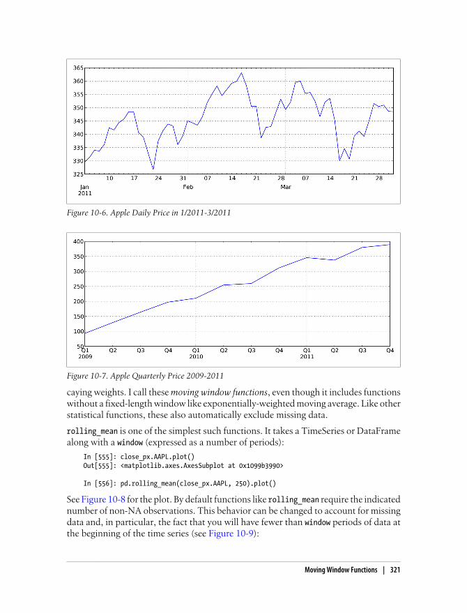
caying weights. I call these moving window functions, even though it includes functionswithout a fixed-length window like exponentially-weighted moving average. Like otherstatistical functions, these also automatically exclude missing data.
rolling_mean is one of the simplest such functions. It takes a TimeSeries or DataFramealong with a window (expressed as a number of periods):
In [555]: close_px.AAPL.plot()Out[555]: <matplotlib.axes.AxesSubplot at 0x1099b3990>
In [556]: pd.rolling_mean(close_px.AAPL, 250).plot()
See Figure 10-8 for the plot. By default functions like rolling_mean require the indicatednumber of non-NA observations. This behavior can be changed to account for missingdata and, in particular, the fact that you will have fewer than window periods of data atthe beginning of the time series (see Figure 10-9):
Figure 10-6. Apple Daily Price in 1/2011-3/2011
Figure 10-7. Apple Quarterly Price 2009-2011
Moving Window Functions | 321
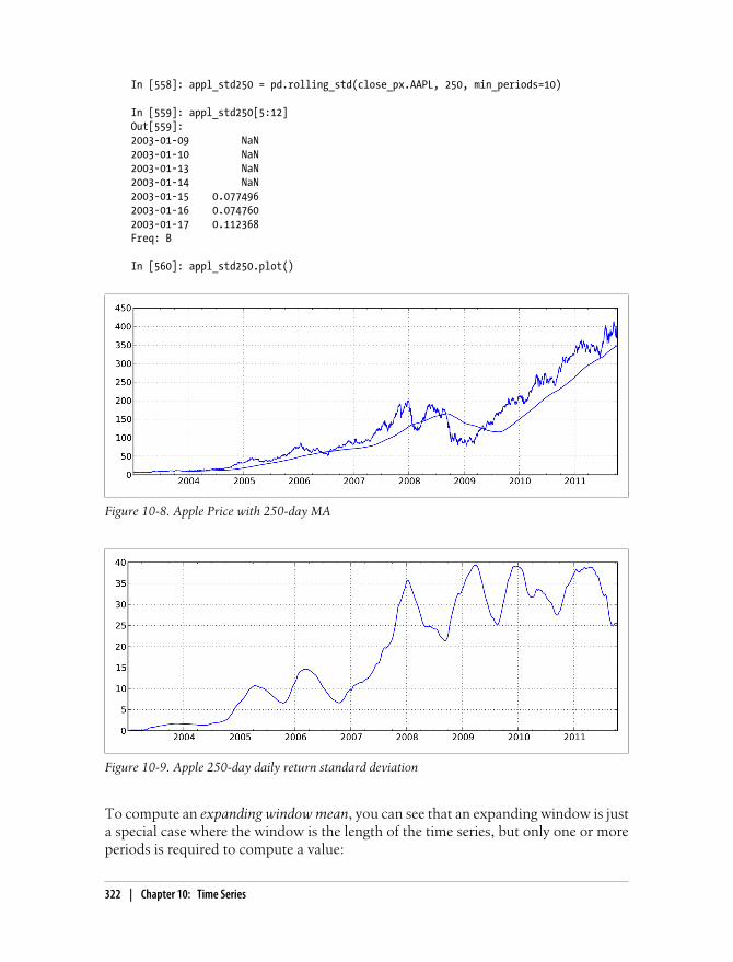
In [558]: appl_std250 = pd.rolling_std(close_px.AAPL, 250, min_periods=10)
In [559]: appl_std250[5:12]Out[559]: 2003-01-09 NaN2003-01-10 NaN2003-01-13 NaN2003-01-14 NaN2003-01-15 0.0774962003-01-16 0.0747602003-01-17 0.112368Freq: B
In [560]: appl_std250.plot()
Figure 10-8. Apple Price with 250-day MA
Figure 10-9. Apple 250-day daily return standard deviation
To compute an expanding window mean, you can see that an expanding window is justa special case where the window is the length of the time series, but only one or moreperiods is required to compute a value:
322 | Chapter 10: Time Series

# Define expanding mean in terms of rolling_meanIn [561]: expanding_mean = lambda x: rolling_mean(x, len(x), min_periods=1)
Calling rolling_mean and friends on a DataFrame applies the transformation to eachcolumn (see Figure 10-10):
In [563]: pd.rolling_mean(close_px, 60).plot(logy=True)
Figure 10-10. Stocks Prices 60-day MA (log Y-axis)
See Table 10-6 for a listing of related functions in pandas.
Table 10-6. Moving window and exponentially-weighted functions
Function Description
rolling_count Returns number of non-NA observations in each trailing window.
rolling_sum Moving window sum.
rolling_mean Moving window mean.
rolling_median Moving window median.
rolling_var, rolling_std Moving window variance and standard deviation, respectively. Uses n - 1 denom-inator.
rolling_skew, rolling_kurt Moving window skewness (3rd moment) and kurtosis (4th moment), respectively.
rolling_min, rolling_max Moving window minimum and maximum.
rolling_quantile Moving window score at percentile/sample quantile.
rolling_corr, rolling_cov Moving window correlation and covariance.
rolling_apply Apply generic array function over a moving window.
ewma Exponentially-weighted moving average.
ewmvar, ewmstd Exponentially-weighted moving variance and standard deviation.
ewmcorr, ewmcov Exponentially-weighted moving correlation and covariance.
Moving Window Functions | 323

bottleneck, a Python library by Keith Goodman, provides an alternateimplementation of NaN-friendly moving window functions and may beworth looking at depending on your application.
Exponentially-weighted functionsAn alternative to using a static window size with equally-weighted observations is tospecify a constant decay factor to give more weight to more recent observations. Inmathematical terms, if mat is the moving average result at time t and x is the time seriesin question, each value in the result is computed as mat = a * mat - 1 + (a - 1) * x_t, wherea is the decay factor. There are a couple of ways to specify the decay factor, a popularone is using a span, which makes the result comparable to a simple moving windowfunction with window size equal to the span.
Since an exponentially-weighted statistic places more weight on more recent observa-tions, it “adapts” faster to changes compared with the equal-weighted version. Here’san example comparing a 60-day moving average of Apple’s stock price with an EWmoving average with span=60 (see Figure 10-11):
fig, axes = plt.subplots(nrows=2, ncols=1, sharex=True, sharey=True, figsize=(12, 7))
aapl_px = close_px.AAPL['2005':'2009']
ma60 = pd.rolling_mean(aapl_px, 60, min_periods=50)ewma60 = pd.ewma(aapl_px, span=60)
aapl_px.plot(style='k-', ax=axes[0])ma60.plot(style='k--', ax=axes[0])aapl_px.plot(style='k-', ax=axes[1])ewma60.plot(style='k--', ax=axes[1])axes[0].set_title('Simple MA')axes[1].set_title('Exponentially-weighted MA')
Binary Moving Window FunctionsSome statistical operators, like correlation and covariance, need to operate on two timeseries. As an example, financial analysts are often interested in a stock’s correlation toa benchmark index like the S&P 500. We can compute that by computing the percentchanges and using rolling_corr (see Figure 10-12):
In [570]: spx_rets = spx_px / spx_px.shift(1) - 1
In [571]: returns = close_px.pct_change()
In [572]: corr = pd.rolling_corr(returns.AAPL, spx_rets, 125, min_periods=100)
In [573]: corr.plot()
324 | Chapter 10: Time Series
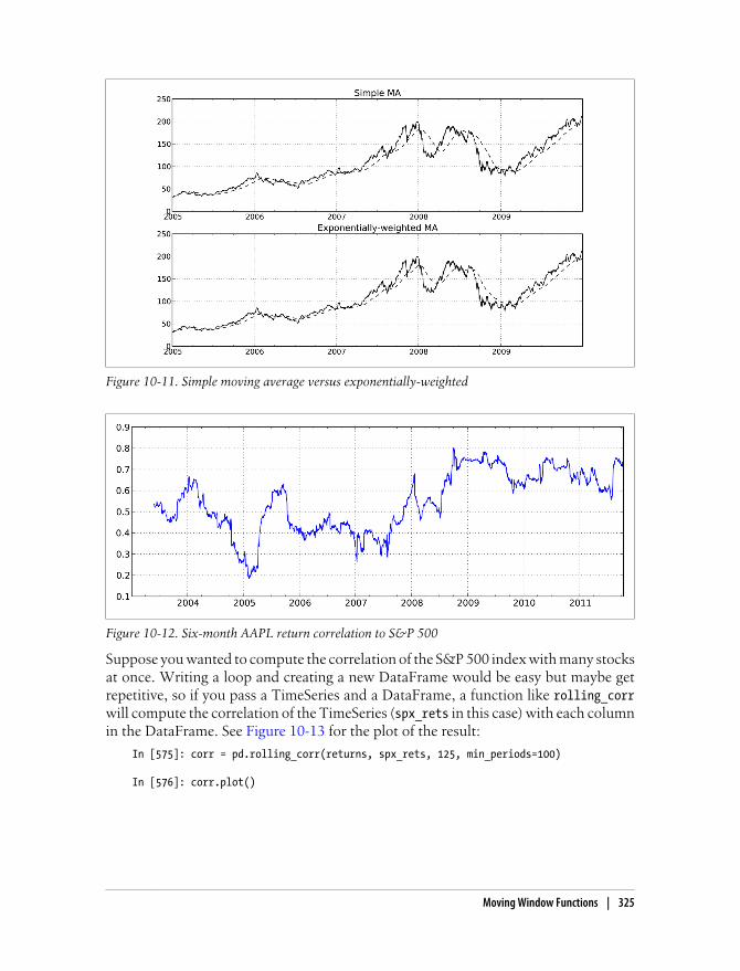
Suppose you wanted to compute the correlation of the S&P 500 index with many stocksat once. Writing a loop and creating a new DataFrame would be easy but maybe getrepetitive, so if you pass a TimeSeries and a DataFrame, a function like rolling_corrwill compute the correlation of the TimeSeries (spx_rets in this case) with each columnin the DataFrame. See Figure 10-13 for the plot of the result:
In [575]: corr = pd.rolling_corr(returns, spx_rets, 125, min_periods=100)
In [576]: corr.plot()
Figure 10-11. Simple moving average versus exponentially-weighted
Figure 10-12. Six-month AAPL return correlation to S&P 500
Moving Window Functions | 325

User-Defined Moving Window FunctionsThe rolling_apply function provides a means to apply an array function of your owndevising over a moving window. The only requirement is that the function produce asingle value (a reduction) from each piece of the array. For example, while we cancompute sample quantiles using rolling_quantile, we might be interested in the per-centile rank of a particular value over the sample. The scipy.stats.percentileofscore function does just this:
In [578]: from scipy.stats import percentileofscore
In [579]: score_at_2percent = lambda x: percentileofscore(x, 0.02)
In [580]: result = pd.rolling_apply(returns.AAPL, 250, score_at_2percent)
In [581]: result.plot()
Figure 10-13. Six-month return correlations to S&P 500
Figure 10-14. Percentile rank of 2% AAPL return over 1 year window
326 | Chapter 10: Time Series
Performance and Memory Usage NotesTimestamps and periods are represented as 64-bit integers using NumPy’s datetime64 dtype. This means that for each data point, there is an associated 8 bytes ofmemory per timestamp. Thus, a time series with 1 million float64 data points has amemory footprint of approximately 16 megabytes. Since pandas makes every effort toshare indexes among time series, creating views on existing time series do not causeany more memory to be used. Additionally, indexes for lower frequencies (daily andup) are stored in a central cache, so that any fixed-frequency index is a view on the datecache. Thus, if you have a large collection of low-frequency time series, the memoryfootprint of the indexes will not be as significant.
Performance-wise, pandas has been highly optimized for data alignment operations(the behind-the-scenes work of differently indexed ts1 + ts2) and resampling. Here isan example of aggregating 10MM data points to OHLC:
In [582]: rng = pd.date_range('1/1/2000', periods=10000000, freq='10ms')
In [583]: ts = Series(np.random.randn(len(rng)), index=rng)
In [584]: tsOut[584]: 2000-01-01 00:00:00 -1.4022352000-01-01 00:00:00.010000 2.4246672000-01-01 00:00:00.020000 -1.9560422000-01-01 00:00:00.030000 -0.897339...2000-01-02 03:46:39.960000 0.4955302000-01-02 03:46:39.970000 0.5747662000-01-02 03:46:39.980000 1.3483742000-01-02 03:46:39.990000 0.665034Freq: 10L, Length: 10000000
In [585]: ts.resample('15min', how='ohlc')Out[585]: <class 'pandas.core.frame.DataFrame'>DatetimeIndex: 113 entries, 2000-01-01 00:00:00 to 2000-01-02 04:00:00Freq: 15TData columns:open 113 non-null valueshigh 113 non-null valueslow 113 non-null valuesclose 113 non-null valuesdtypes: float64(4)
In [586]: %timeit ts.resample('15min', how='ohlc')10 loops, best of 3: 61.1 ms per loop
The runtime may depend slightly on the relative size of the aggregated result; higherfrequency aggregates unsurprisingly take longer to compute:
In [587]: rng = pd.date_range('1/1/2000', periods=10000000, freq='1s')
Performance and Memory Usage Notes | 327

In [588]: ts = Series(np.random.randn(len(rng)), index=rng)
In [589]: %timeit ts.resample('15s', how='ohlc')1 loops, best of 3: 88.2 ms per loop
It’s possible that by the time you read this, the performance of these algorithms maybe even further improved. As an example, there are currently no optimizations forconversions between regular frequencies, but that would be fairly straightforward to do.
328 | Chapter 10: Time Series

CHAPTER 11
Financial and Economic DataApplications
The use of Python in the financial industry has been increasing rapidly since 2005, ledlargely by the maturation of libraries (like NumPy and pandas) and the availability ofskilled Python programmers. Institutions have found that Python is well-suited bothas an interactive analysis environment as well as enabling robust systems to be devel-oped often in a fraction of the time it would have taken in Java or C++. Python is alsoan ideal glue layer; it is easy to build Python interfaces to legacy libraries built in C orC++.
While the field of financial analysis is broad enough to fill an entire book, I hope toshow you how the tools in this book can be applied to a number of specific problemsin finance. As with other research and analysis domains, too much programming effortis often spent wrangling data rather than solving the core modeling and research prob-lems. I personally got started building pandas in 2008 while grappling with inadequatedata tools.
In these examples, I’ll use the term cross-section to refer to data at a fixed point in time.For example, the closing prices of all the stocks in the S&P 500 index on a particulardate form a cross-section. Cross-sectional data at multiple points in time over multipledata items (for example, prices together with volume) form a panel. Panel data caneither be represented as a hierarchically-indexed DataFrame or using the three-dimen-sional Panel pandas object.
Data Munging TopicsMany helpful data munging tools for financial applications are spread across the earlierchapters. Here I’ll highlight a number of topics as they relate to this problem domain.
329

Time Series and Cross-Section AlignmentOne of the most time-consuming issues in working with financial data is the so-calleddata alignment problem. Two related time series may have indexes that don’t line upperfectly, or two DataFrame objects might have columns or row labels that don’t match.Users of MATLAB, R, and other matrix-programming languages often invest significanteffort in wrangling data into perfectly aligned forms. In my experience, having to aligndata by hand (and worse, having to verify that data is aligned) is a far too rigid andtedious way to work. It is also rife with potential for bugs due to combining misaligneddata.
pandas take an alternate approach by automatically aligning data in arithmetic opera-tions. In practice, this grants immense freedom and enhances your productivity. As anexample, let’s consider a couple of DataFrames containing time series of stock pricesand volume:
In [16]: pricesOut[16]: AAPL JNJ SPX XOM2011-09-06 379.74 64.64 1165.24 71.152011-09-07 383.93 65.43 1198.62 73.652011-09-08 384.14 64.95 1185.90 72.822011-09-09 377.48 63.64 1154.23 71.012011-09-12 379.94 63.59 1162.27 71.842011-09-13 384.62 63.61 1172.87 71.652011-09-14 389.30 63.73 1188.68 72.64
In [17]: volumeOut[17]: AAPL JNJ XOM2011-09-06 18173500 15848300 254163002011-09-07 12492000 10759700 231084002011-09-08 14839800 15551500 224348002011-09-09 20171900 17008200 279691002011-09-12 16697300 13448200 26205800
Suppose you wanted to compute a volume-weighted average price using all availabledata (and making the simplifying assumption that the volume data is a subset of theprice data). Since pandas aligns the data automatically in arithmetic and excludesmissing data in functions like sum, we can express this concisely as:
In [18]: prices * volumeOut[18]: AAPL JNJ SPX XOM2011-09-06 6901204890 1024434112 NaN 18083697452011-09-07 4796053560 704007171 NaN 17019336602011-09-08 5700560772 1010069925 NaN 16337021362011-09-09 7614488812 1082401848 NaN 19860857912011-09-12 6343972162 855171038 NaN 18826246722011-09-13 NaN NaN NaN NaN2011-09-14 NaN NaN NaN NaN
In [19]: vwap = (prices * volume).sum() / volume.sum()
330 | Chapter 11: Financial and Economic Data Applications

In [20]: vwap In [21]: vwap.dropna()Out[20]: Out[21]: AAPL 380.655181 AAPL 380.655181 JNJ 64.394769 JNJ 64.394769 SPX NaN XOM 72.024288 XOM 72.024288
Since SPX wasn’t found in volume, you can choose to explicitly discard that at any point.Should you wish to align by hand, you can use DataFrame’s align method, whichreturns a tuple of reindexed versions of the two objects:
In [22]: prices.align(volume, join='inner')Out[22]: ( AAPL JNJ XOM2011-09-06 379.74 64.64 71.152011-09-07 383.93 65.43 73.652011-09-08 384.14 64.95 72.822011-09-09 377.48 63.64 71.012011-09-12 379.94 63.59 71.84, AAPL JNJ XOM2011-09-06 18173500 15848300 254163002011-09-07 12492000 10759700 231084002011-09-08 14839800 15551500 224348002011-09-09 20171900 17008200 279691002011-09-12 16697300 13448200 26205800)
Another indispensable feature is constructing a DataFrame from a collection of poten-tially differently indexed Series:
In [23]: s1 = Series(range(3), index=['a', 'b', 'c'])
In [24]: s2 = Series(range(4), index=['d', 'b', 'c', 'e'])
In [25]: s3 = Series(range(3), index=['f', 'a', 'c'])
In [26]: DataFrame({'one': s1, 'two': s2, 'three': s3})Out[26]: one three twoa 0 1 NaNb 1 NaN 1c 2 2 2d NaN NaN 0e NaN NaN 3f NaN 0 NaN
As you have seen earlier, you can of course specify explicitly the index of the result,discarding the rest of the data:
In [27]: DataFrame({'one': s1, 'two': s2, 'three': s3}, index=list('face'))Out[27]: one three twof NaN 0 NaNa 0 1 NaNc 2 2 2e NaN NaN 3
Data Munging Topics | 331
Operations with Time Series of Different FrequenciesEconomic time series are often of annual, quarterly, monthly, daily, or some other morespecialized frequency. Some are completely irregular; for example, earnings revisionsfor a stock may arrive at any time. The two main tools for frequency conversion andrealignment are the resample and reindex methods. resample converts data to a fixedfrequency while reindex conforms data to a new index. Both support optional inter-polation (such as forward filling) logic.
Let’s consider a small weekly time series:
In [28]: ts1 = Series(np.random.randn(3), ....: index=pd.date_range('2012-6-13', periods=3, freq='W-WED'))
In [29]: ts1Out[29]: 2012-06-13 -1.1248012012-06-20 0.4690042012-06-27 -0.117439Freq: W-WED
If you resample this to business daily (Monday-Friday) frequency, you get holes on thedays where there is no data:
In [30]: ts1.resample('B')Out[30]: 2012-06-13 -1.1248012012-06-14 NaN2012-06-15 NaN2012-06-18 NaN2012-06-19 NaN2012-06-20 0.4690042012-06-21 NaN2012-06-22 NaN2012-06-25 NaN2012-06-26 NaN2012-06-27 -0.117439Freq: B
Of course, using 'ffill' as the fill_method forward fills values in those gaps. This isa common practice with lower frequency data as you compute a time series of valueson each timestamp having the latest valid or “as of” value:
In [31]: ts1.resample('B', fill_method='ffill')Out[31]: 2012-06-13 -1.1248012012-06-14 -1.1248012012-06-15 -1.1248012012-06-18 -1.1248012012-06-19 -1.1248012012-06-20 0.4690042012-06-21 0.4690042012-06-22 0.4690042012-06-25 0.4690042012-06-26 0.469004
332 | Chapter 11: Financial and Economic Data Applications

2012-06-27 -0.117439Freq: B
In practice, upsampling lower frequency data to a higher, regular frequency is a finesolution, but in the more general irregular time series case it may be a poor fit. Consideran irregularly sampled time series from the same general time period:
In [32]: dates = pd.DatetimeIndex(['2012-6-12', '2012-6-17', '2012-6-18', ....: '2012-6-21', '2012-6-22', '2012-6-29'])
In [33]: ts2 = Series(np.random.randn(6), index=dates)
In [34]: ts2Out[34]: 2012-06-12 -0.4494292012-06-17 0.4596482012-06-18 -0.1725312012-06-21 0.8359382012-06-22 -0.5947792012-06-29 0.027197
If you wanted to add the “as of” values in ts1 (forward filling) to ts2. One option wouldbe to resample both to a regular frequency then add, but if you want to maintain thedate index in ts2, using reindex is a more precise solution:
In [35]: ts1.reindex(ts2.index, method='ffill')Out[35]: 2012-06-12 NaN2012-06-17 -1.1248012012-06-18 -1.1248012012-06-21 0.4690042012-06-22 0.4690042012-06-29 -0.117439
In [36]: ts2 + ts1.reindex(ts2.index, method='ffill')Out[36]: 2012-06-12 NaN2012-06-17 -0.6651532012-06-18 -1.2973322012-06-21 1.3049422012-06-22 -0.1257752012-06-29 -0.090242
Using periods instead of timestamps
Periods (representing time spans) provide an alternate means of working with differentfrequency time series, especially financial or economic series with annual or quarterlyfrequency having a particular reporting convention. For example, a company mightannounce its quarterly earnings with fiscal year ending in June, thus having Q-JUN fre-quency. Consider a pair of macroeconomic time series related to GDP and inflation:
In [37]: gdp = Series([1.78, 1.94, 2.08, 2.01, 2.15, 2.31, 2.46], ....: index=pd.period_range('1984Q2', periods=7, freq='Q-SEP'))
Data Munging Topics | 333
In [38]: infl = Series([0.025, 0.045, 0.037, 0.04], ....: index=pd.period_range('1982', periods=4, freq='A-DEC'))
In [39]: gdp In [40]: inflOut[39]: Out[40]: 1984Q2 1.78 1982 0.0251984Q3 1.94 1983 0.0451984Q4 2.08 1984 0.0371985Q1 2.01 1985 0.0401985Q2 2.15 Freq: A-DEC 1985Q3 2.31 1985Q4 2.46 Freq: Q-SEP
Unlike time series with timestamps, operations between different-frequency time seriesindexed by periods are not possible without explicit conversions. In this case, if weknow that infl values were observed at the end of each year, we can then convert toQ-SEP to get the right periods in that frequency:
In [41]: infl_q = infl.asfreq('Q-SEP', how='end')
In [42]: infl_qOut[42]: 1983Q1 0.0251984Q1 0.0451985Q1 0.0371986Q1 0.040Freq: Q-SEP
That time series can then be reindexed with forward-filling to match gdp:
In [43]: infl_q.reindex(gdp.index, method='ffill')Out[43]: 1984Q2 0.0451984Q3 0.0451984Q4 0.0451985Q1 0.0371985Q2 0.0371985Q3 0.0371985Q4 0.037Freq: Q-SEP
Time of Day and “as of” Data SelectionSuppose you have a long time series containing intraday market data and you want toextract the prices at a particular time of day on each day of the data. What if the dataare irregular such that observations do not fall exactly on the desired time? In practicethis task can make for error-prone data munging if you are not careful. Here is anexample for illustration purposes:
# Make an intraday date range and time seriesIn [44]: rng = pd.date_range('2012-06-01 09:30', '2012-06-01 15:59', freq='T')
# Make a 5-day series of 9:30-15:59 values
334 | Chapter 11: Financial and Economic Data Applications
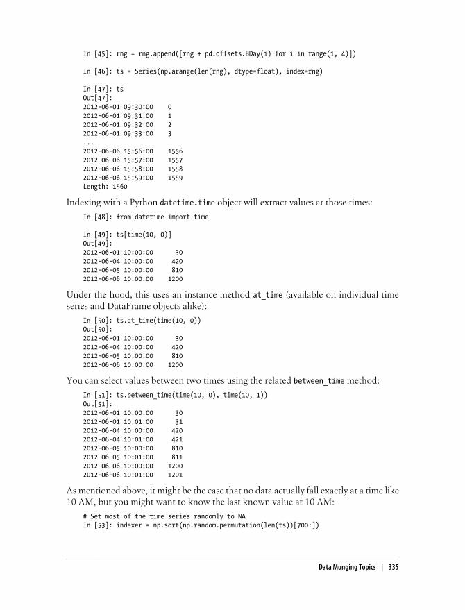
In [45]: rng = rng.append([rng + pd.offsets.BDay(i) for i in range(1, 4)])
In [46]: ts = Series(np.arange(len(rng), dtype=float), index=rng)
In [47]: tsOut[47]: 2012-06-01 09:30:00 02012-06-01 09:31:00 12012-06-01 09:32:00 22012-06-01 09:33:00 3...2012-06-06 15:56:00 15562012-06-06 15:57:00 15572012-06-06 15:58:00 15582012-06-06 15:59:00 1559Length: 1560
Indexing with a Python datetime.time object will extract values at those times:
In [48]: from datetime import time
In [49]: ts[time(10, 0)]Out[49]: 2012-06-01 10:00:00 302012-06-04 10:00:00 4202012-06-05 10:00:00 8102012-06-06 10:00:00 1200
Under the hood, this uses an instance method at_time (available on individual timeseries and DataFrame objects alike):
In [50]: ts.at_time(time(10, 0))Out[50]: 2012-06-01 10:00:00 302012-06-04 10:00:00 4202012-06-05 10:00:00 8102012-06-06 10:00:00 1200
You can select values between two times using the related between_time method:
In [51]: ts.between_time(time(10, 0), time(10, 1))Out[51]: 2012-06-01 10:00:00 302012-06-01 10:01:00 312012-06-04 10:00:00 4202012-06-04 10:01:00 4212012-06-05 10:00:00 8102012-06-05 10:01:00 8112012-06-06 10:00:00 12002012-06-06 10:01:00 1201
As mentioned above, it might be the case that no data actually fall exactly at a time like10 AM, but you might want to know the last known value at 10 AM:
# Set most of the time series randomly to NAIn [53]: indexer = np.sort(np.random.permutation(len(ts))[700:])
Data Munging Topics | 335

In [54]: irr_ts = ts.copy()
In [55]: irr_ts[indexer] = np.nan
In [56]: irr_ts['2012-06-01 09:50':'2012-06-01 10:00']Out[56]: 2012-06-01 09:50:00 202012-06-01 09:51:00 NaN2012-06-01 09:52:00 222012-06-01 09:53:00 232012-06-01 09:54:00 NaN2012-06-01 09:55:00 252012-06-01 09:56:00 NaN2012-06-01 09:57:00 NaN2012-06-01 09:58:00 NaN2012-06-01 09:59:00 NaN2012-06-01 10:00:00 NaN
By passing an array of timestamps to the asof method, you will obtain an array of thelast valid (non-NA) values at or before each timestamp. So we construct a date rangeat 10 AM for each day and pass that to asof:
In [57]: selection = pd.date_range('2012-06-01 10:00', periods=4, freq='B')
In [58]: irr_ts.asof(selection)Out[58]: 2012-06-01 10:00:00 252012-06-04 10:00:00 4202012-06-05 10:00:00 8102012-06-06 10:00:00 1197Freq: B
Splicing Together Data SourcesIn Chapter 7, I described a number of strategies for merging together two related datasets. In a financial or economic context, there are a few widely occurring use cases:
• Switching from one data source (a time series or collection of time series) to anotherat a specific point in time
• “Patching” missing values in a time series at the beginning, middle, or end usinganother time series
• Completely replacing the data for a subset of symbols (countries, asset tickers, andso on)
In the first case, switching from one set of time series to another at a specific instant, itis a matter of splicing together two TimeSeries or DataFrame objects using pandas.concat:
In [59]: data1 = DataFrame(np.ones((6, 3), dtype=float), ....: columns=['a', 'b', 'c'], ....: index=pd.date_range('6/12/2012', periods=6))
336 | Chapter 11: Financial and Economic Data Applications

In [60]: data2 = DataFrame(np.ones((6, 3), dtype=float) * 2, ....: columns=['a', 'b', 'c'], ....: index=pd.date_range('6/13/2012', periods=6))
In [61]: spliced = pd.concat([data1.ix[:'2012-06-14'], data2.ix['2012-06-15':]])
In [62]: splicedOut[62]: a b c2012-06-12 1 1 12012-06-13 1 1 12012-06-14 1 1 12012-06-15 2 2 22012-06-16 2 2 22012-06-17 2 2 22012-06-18 2 2 2
Suppose in a similar example that data1 was missing a time series present in data2:
In [63]: data2 = DataFrame(np.ones((6, 4), dtype=float) * 2, ....: columns=['a', 'b', 'c', 'd'], ....: index=pd.date_range('6/13/2012', periods=6))
In [64]: spliced = pd.concat([data1.ix[:'2012-06-14'], data2.ix['2012-06-15':]])
In [65]: splicedOut[65]: a b c d2012-06-12 1 1 1 NaN2012-06-13 1 1 1 NaN2012-06-14 1 1 1 NaN2012-06-15 2 2 2 22012-06-16 2 2 2 22012-06-17 2 2 2 22012-06-18 2 2 2 2
Using combine_first, you can bring in data from before the splice point to extend thehistory for 'd' item:
In [66]: spliced_filled = spliced.combine_first(data2)
In [67]: spliced_filledOut[67]: a b c d2012-06-12 1 1 1 NaN2012-06-13 1 1 1 22012-06-14 1 1 1 22012-06-15 2 2 2 22012-06-16 2 2 2 22012-06-17 2 2 2 22012-06-18 2 2 2 2
Since data2 does not have any values for 2012-06-12, no values are filled on that day.
DataFrame has a related method update for performing in-place updates. You have topass overwrite=False to make it only fill the holes:
Data Munging Topics | 337
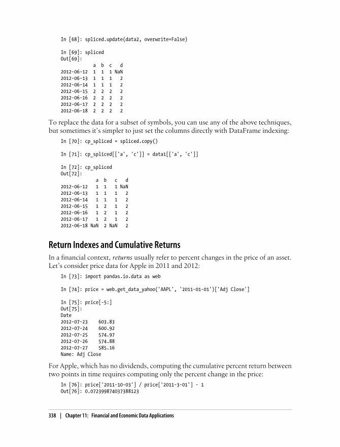
In [68]: spliced.update(data2, overwrite=False)
In [69]: splicedOut[69]: a b c d2012-06-12 1 1 1 NaN2012-06-13 1 1 1 22012-06-14 1 1 1 22012-06-15 2 2 2 22012-06-16 2 2 2 22012-06-17 2 2 2 22012-06-18 2 2 2 2
To replace the data for a subset of symbols, you can use any of the above techniques,but sometimes it’s simpler to just set the columns directly with DataFrame indexing:
In [70]: cp_spliced = spliced.copy()
In [71]: cp_spliced[['a', 'c']] = data1[['a', 'c']]
In [72]: cp_splicedOut[72]: a b c d2012-06-12 1 1 1 NaN2012-06-13 1 1 1 22012-06-14 1 1 1 22012-06-15 1 2 1 22012-06-16 1 2 1 22012-06-17 1 2 1 22012-06-18 NaN 2 NaN 2
Return Indexes and Cumulative ReturnsIn a financial context, returns usually refer to percent changes in the price of an asset.Let’s consider price data for Apple in 2011 and 2012:
In [73]: import pandas.io.data as web
In [74]: price = web.get_data_yahoo('AAPL', '2011-01-01')['Adj Close']
In [75]: price[-5:]Out[75]: Date2012-07-23 603.832012-07-24 600.922012-07-25 574.972012-07-26 574.882012-07-27 585.16Name: Adj Close
For Apple, which has no dividends, computing the cumulative percent return betweentwo points in time requires computing only the percent change in the price:
In [76]: price['2011-10-03'] / price['2011-3-01'] - 1Out[76]: 0.072399874037388123
338 | Chapter 11: Financial and Economic Data Applications
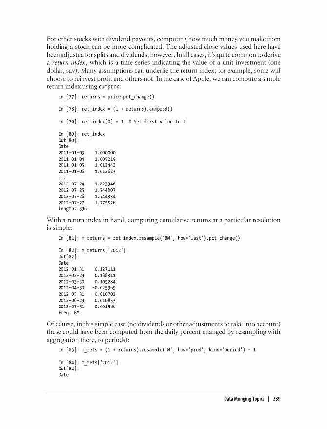
For other stocks with dividend payouts, computing how much money you make fromholding a stock can be more complicated. The adjusted close values used here havebeen adjusted for splits and dividends, however. In all cases, it’s quite common to derivea return index, which is a time series indicating the value of a unit investment (onedollar, say). Many assumptions can underlie the return index; for example, some willchoose to reinvest profit and others not. In the case of Apple, we can compute a simplereturn index using cumprod:
In [77]: returns = price.pct_change()
In [78]: ret_index = (1 + returns).cumprod()
In [79]: ret_index[0] = 1 # Set first value to 1
In [80]: ret_indexOut[80]: Date2011-01-03 1.0000002011-01-04 1.0052192011-01-05 1.0134422011-01-06 1.012623...2012-07-24 1.8233462012-07-25 1.7446072012-07-26 1.7443342012-07-27 1.775526Length: 396
With a return index in hand, computing cumulative returns at a particular resolutionis simple:
In [81]: m_returns = ret_index.resample('BM', how='last').pct_change()
In [82]: m_returns['2012']Out[82]: Date2012-01-31 0.1271112012-02-29 0.1883112012-03-30 0.1052842012-04-30 -0.0259692012-05-31 -0.0107022012-06-29 0.0108532012-07-31 0.001986Freq: BM
Of course, in this simple case (no dividends or other adjustments to take into account)these could have been computed from the daily percent changed by resampling withaggregation (here, to periods):
In [83]: m_rets = (1 + returns).resample('M', how='prod', kind='period') - 1
In [84]: m_rets['2012']Out[84]: Date
Data Munging Topics | 339

2012-01 0.1271112012-02 0.1883112012-03 0.1052842012-04 -0.0259692012-05 -0.0107022012-06 0.0108532012-07 0.001986Freq: M
If you had dividend dates and percentages, including them in the total return per daywould look like:
returns[dividend_dates] += dividend_pcts
Group Transforms and AnalysisIn Chapter 9, you learned the basics of computing group statistics and applying yourown transformations to groups in a dataset.
Let’s consider a collection of hypothetical stock portfolios. I first randomly generate abroad universe of 2000 tickers:
import random; random.seed(0)import string
N = 1000def rands(n): choices = string.ascii_uppercase return ''.join([random.choice(choices) for _ in xrange(n)])tickers = np.array([rands(5) for _ in xrange(N)])
I then create a DataFrame containing 3 columns representing hypothetical, but randomportfolios for a subset of tickers:
M = 500df = DataFrame({'Momentum' : np.random.randn(M) / 200 + 0.03, 'Value' : np.random.randn(M) / 200 + 0.08, 'ShortInterest' : np.random.randn(M) / 200 - 0.02}, index=tickers[:M])
Next, let’s create a random industry classification for the tickers. To keep things simple,I’ll just keep it to 2 industries, storing the mapping in a Series:
ind_names = np.array(['FINANCIAL', 'TECH'])sampler = np.random.randint(0, len(ind_names), N)industries = Series(ind_names[sampler], index=tickers, name='industry')
Now we can group by industries and carry out group aggregation and transformations:
In [90]: by_industry = df.groupby(industries)
In [91]: by_industry.mean()Out[91]: Momentum ShortInterest Value
340 | Chapter 11: Financial and Economic Data Applications
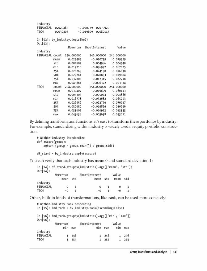
industry FINANCIAL 0.029485 -0.020739 0.079929TECH 0.030407 -0.019609 0.080113
In [92]: by_industry.describe()Out[92]: Momentum ShortInterest Valueindustry FINANCIAL count 246.000000 246.000000 246.000000 mean 0.029485 -0.020739 0.079929 std 0.004802 0.004986 0.004548 min 0.017210 -0.036997 0.067025 25% 0.026263 -0.024138 0.076638 50% 0.029261 -0.020833 0.079804 75% 0.032806 -0.017345 0.082718 max 0.045884 -0.006322 0.093334TECH count 254.000000 254.000000 254.000000 mean 0.030407 -0.019609 0.080113 std 0.005303 0.005074 0.004886 min 0.016778 -0.032682 0.065253 25% 0.026456 -0.022779 0.076737 50% 0.030650 -0.019829 0.080296 75% 0.033602 -0.016923 0.083353 max 0.049638 -0.003698 0.093081
By defining transformation functions, it’s easy to transform these portfolios by industry.For example, standardizing within industry is widely used in equity portfolio construc-tion:
# Within-Industry Standardizedef zscore(group): return (group - group.mean()) / group.std()
df_stand = by_industry.apply(zscore)
You can verify that each industry has mean 0 and standard deviation 1:
In [94]: df_stand.groupby(industries).agg(['mean', 'std'])Out[94]: Momentum ShortInterest Value mean std mean std mean stdindustry FINANCIAL 0 1 0 1 0 1TECH -0 1 -0 1 -0 1
Other, built-in kinds of transformations, like rank, can be used more concisely:
# Within-industry rank descendingIn [95]: ind_rank = by_industry.rank(ascending=False)
In [96]: ind_rank.groupby(industries).agg(['min', 'max'])Out[96]: Momentum ShortInterest Value min max min max min maxindustry FINANCIAL 1 246 1 246 1 246TECH 1 254 1 254 1 254
Group Transforms and Analysis | 341

In quantitative equity, “rank and standardize” is a common sequence of transforms.You could do this by chaining together rank and zscore like so:
# Industry rank and standardizeIn [97]: by_industry.apply(lambda x: zscore(x.rank()))Out[97]: <class 'pandas.core.frame.DataFrame'>Index: 500 entries, VTKGN to PTDQEData columns:Momentum 500 non-null valuesShortInterest 500 non-null valuesValue 500 non-null valuesdtypes: float64(3)
Group Factor ExposuresFactor analysis is a technique in quantitative portfolio management. Portfolio holdingsand performance (profit and less) are decomposed using one or more factors (risk fac-tors are one example) represented as a portfolio of weights. For example, a stock price’sco-movement with a benchmark (like S&P 500 index) is known as its beta, a commonrisk factor. Let’s consider a contrived example of a portfolio constructed from 3 ran-domly-generated factors (usually called the factor loadings) and some weights:
from numpy.random import randfac1, fac2, fac3 = np.random.rand(3, 1000)
ticker_subset = tickers.take(np.random.permutation(N)[:1000])
# Weighted sum of factors plus noiseport = Series(0.7 * fac1 - 1.2 * fac2 + 0.3 * fac3 + rand(1000), index=ticker_subset)factors = DataFrame({'f1': fac1, 'f2': fac2, 'f3': fac3}, index=ticker_subset)
Vector correlations between each factor and the portfolio may not indicate too much:
In [99]: factors.corrwith(port)Out[99]: f1 0.402377f2 -0.680980f3 0.168083
The standard way to compute the factor exposures is by least squares regression; usingpandas.ols with factors as the explanatory variables we can compute exposures overthe entire set of tickers:
In [100]: pd.ols(y=port, x=factors).betaOut[100]: f1 0.761789f2 -1.208760f3 0.289865intercept 0.484477
342 | Chapter 11: Financial and Economic Data Applications

As you can see, the original factor weights can nearly be recovered since there was nottoo much additional random noise added to the portfolio. Using groupby you can com-pute exposures industry by industry. To do so, write a function like so:
def beta_exposure(chunk, factors=None): return pd.ols(y=chunk, x=factors).beta
Then, group by industries and apply that function, passing the DataFrame of factorloadings:
In [102]: by_ind = port.groupby(industries)
In [103]: exposures = by_ind.apply(beta_exposure, factors=factors)
In [104]: exposures.unstack()Out[104]: f1 f2 f3 interceptindustry FINANCIAL 0.790329 -1.182970 0.275624 0.455569TECH 0.740857 -1.232882 0.303811 0.508188
Decile and Quartile AnalysisAnalyzing data based on sample quantiles is another important tool for financial ana-lysts. For example, the performance of a stock portfolio could be broken down intoquartiles (four equal-sized chunks) based on each stock’s price-to-earnings. Using pandas.qcut combined with groupby makes quantile analysis reasonably straightforward.
As an example, let’s consider a simple trend following or momentum strategy tradingthe S&P 500 index via the SPY exchange-traded fund. You can download the pricehistory from Yahoo! Finance:
In [105]: import pandas.io.data as web
In [106]: data = web.get_data_yahoo('SPY', '2006-01-01')
In [107]: dataOut[107]: <class 'pandas.core.frame.DataFrame'>DatetimeIndex: 1655 entries, 2006-01-03 00:00:00 to 2012-07-27 00:00:00Data columns:Open 1655 non-null valuesHigh 1655 non-null valuesLow 1655 non-null valuesClose 1655 non-null valuesVolume 1655 non-null valuesAdj Close 1655 non-null valuesdtypes: float64(5), int64(1)
Now, we’ll compute daily returns and a function for transforming the returns into atrend signal formed from a lagged moving sum:
px = data['Adj Close']returns = px.pct_change()
Group Transforms and Analysis | 343
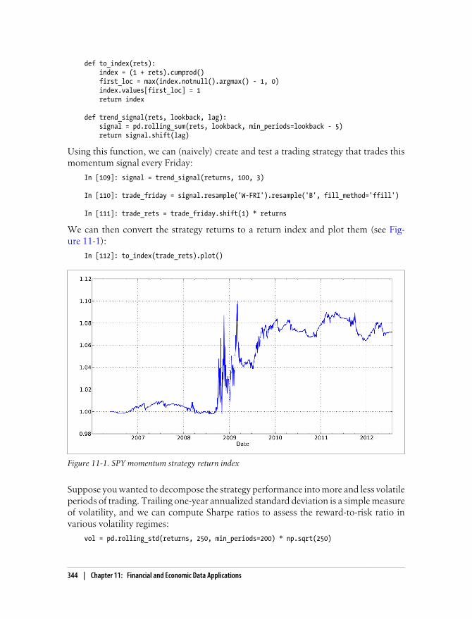
def to_index(rets): index = (1 + rets).cumprod() first_loc = max(index.notnull().argmax() - 1, 0) index.values[first_loc] = 1 return index
def trend_signal(rets, lookback, lag): signal = pd.rolling_sum(rets, lookback, min_periods=lookback - 5) return signal.shift(lag)
Using this function, we can (naively) create and test a trading strategy that trades thismomentum signal every Friday:
In [109]: signal = trend_signal(returns, 100, 3)
In [110]: trade_friday = signal.resample('W-FRI').resample('B', fill_method='ffill')
In [111]: trade_rets = trade_friday.shift(1) * returns
We can then convert the strategy returns to a return index and plot them (see Fig-ure 11-1):
In [112]: to_index(trade_rets).plot()
Figure 11-1. SPY momentum strategy return index
Suppose you wanted to decompose the strategy performance into more and less volatileperiods of trading. Trailing one-year annualized standard deviation is a simple measureof volatility, and we can compute Sharpe ratios to assess the reward-to-risk ratio invarious volatility regimes:
vol = pd.rolling_std(returns, 250, min_periods=200) * np.sqrt(250)
344 | Chapter 11: Financial and Economic Data Applications

def sharpe(rets, ann=250): return rets.mean() / rets.std() * np.sqrt(ann)
Now, dividing vol into quartiles with qcut and aggregating with sharpe we obtain:
In [114]: trade_rets.groupby(pd.qcut(vol, 4)).agg(sharpe)Out[114]: [0.0955, 0.16] 0.490051(0.16, 0.188] 0.482788(0.188, 0.231] -0.731199(0.231, 0.457] 0.570500
These results show that the strategy performed the best during the period when thevolatility was the highest.
More Example ApplicationsHere is a small set of additional examples.
Signal Frontier AnalysisIn this section, I’ll describe a simplified cross-sectional momentum portfolio and showhow you might explore a grid of model parameterizations. First, I’ll load historicalprices for a portfolio of financial and technology stocks:
names = ['AAPL', 'GOOG', 'MSFT', 'DELL', 'GS', 'MS', 'BAC', 'C']def get_px(stock, start, end): return web.get_data_yahoo(stock, start, end)['Adj Close']px = DataFrame({n: get_px(n, '1/1/2009', '6/1/2012') for n in names})
We can easily plot the cumulative returns of each stock (see Figure 11-2):
In [117]: px = px.asfreq('B').fillna(method='pad')
In [118]: rets = px.pct_change()
In [119]: ((1 + rets).cumprod() - 1).plot()
For the portfolio construction, we’ll compute momentum over a certain lookback, thenrank in descending order and standardize:
def calc_mom(price, lookback, lag): mom_ret = price.shift(lag).pct_change(lookback) ranks = mom_ret.rank(axis=1, ascending=False) demeaned = ranks - ranks.mean(axis=1) return demeaned / demeaned.std(axis=1)
With this transform function in hand, we can set up a strategy backtesting functionthat computes a portfolio for a particular lookback and holding period (days betweentrading), returning the overall Sharpe ratio:
compound = lambda x : (1 + x).prod() - 1daily_sr = lambda x: x.mean() / x.std()
More Example Applications | 345

def strat_sr(prices, lb, hold): # Compute portfolio weights freq = '%dB' % hold port = calc_mom(prices, lb, lag=1)
daily_rets = prices.pct_change()
# Compute portfolio returns port = port.shift(1).resample(freq, how='first') returns = daily_rets.resample(freq, how=compound) port_rets = (port * returns).sum(axis=1)
return daily_sr(port_rets) * np.sqrt(252 / hold)
Figure 11-2. Cumulative returns for each of the stocks
When called with the prices and a parameter combination, this function returns a scalarvalue:
In [122]: strat_sr(px, 70, 30)Out[122]: 0.27421582756800583
From there, you can evaluate the strat_sr function over a grid of parameters, storingthem as you go in a defaultdict and finally putting the results in a DataFrame:
from collections import defaultdict
lookbacks = range(20, 90, 5)holdings = range(20, 90, 5)dd = defaultdict(dict)for lb in lookbacks: for hold in holdings: dd[lb][hold] = strat_sr(px, lb, hold)
346 | Chapter 11: Financial and Economic Data Applications

ddf = DataFrame(dd)ddf.index.name = 'Holding Period'ddf.columns.name = 'Lookback Period'
To visualize the results and get an idea of what’s going on, here is a function that usesmatplotlib to produce a heatmap with some adornments:
import matplotlib.pyplot as plt
def heatmap(df, cmap=plt.cm.gray_r): fig = plt.figure() ax = fig.add_subplot(111) axim = ax.imshow(df.values, cmap=cmap, interpolation='nearest') ax.set_xlabel(df.columns.name) ax.set_xticks(np.arange(len(df.columns))) ax.set_xticklabels(list(df.columns)) ax.set_ylabel(df.index.name) ax.set_yticks(np.arange(len(df.index))) ax.set_yticklabels(list(df.index)) plt.colorbar(axim)
Calling this function on the backtest results, we get Figure 11-3:
In [125]: heatmap(ddf)
Figure 11-3. Heatmap of momentum strategy Sharpe ratio (higher is better) over various lookbacksand holding periods
Future Contract RollingA future is an ubiquitous form of derivative contract; it is an agreement to take deliveryof a certain asset (such as oil, gold, or shares of the FTSE 100 index) on a particulardate. In practice, modeling and trading futures contracts on equities, currencies,
More Example Applications | 347
commodities, bonds, and other asset classes is complicated by the time-limited natureof each contract. For example, at any given time for a type of future (say silver or copperfutures) multiple contracts with different expiration dates may be traded. In many cases,the future contract expiring next (the near contract) will be the most liquid (highestvolume and lowest bid-ask spread).
For the purposes of modeling and forecasting, it can be much easier to work with a continuous return index indicating the profit and loss associated with always holdingthe near contract. Transitioning from an expiring contract to the next (or far) contractis referred to as rolling. Computing a continuous future series from the individual con-tract data is not necessarily a straightforward exercise and typically requires a deeperunderstanding of the market and how the instruments are traded. For example, inpractice when and how quickly would you trade out of an expiring contract and intothe next contract? Here I describe one such process.
First, I’ll use scaled prices for the SPY exchange-traded fund as a proxy for the S&P 500index:
In [127]: import pandas.io.data as web
# Approximate price of S&P 500 indexIn [128]: px = web.get_data_yahoo('SPY')['Adj Close'] * 10
In [129]: pxOut[129]: Date2011-08-01 1261.02011-08-02 1228.82011-08-03 1235.5...2012-07-25 1339.62012-07-26 1361.72012-07-27 1386.8Name: Adj Close, Length: 251
Now, a little bit of setup. I put a couple of S&P 500 future contracts and expiry datesin a Series:
from datetime import datetimeexpiry = {'ESU2': datetime(2012, 9, 21), 'ESZ2': datetime(2012, 12, 21)}expiry = Series(expiry).order()
expiry then looks like:
In [131]: expiryOut[131]: ESU2 2012-09-21 00:00:00ESZ2 2012-12-21 00:00:00
348 | Chapter 11: Financial and Economic Data Applications

Then, I use the Yahoo! Finance prices along with a random walk and some noise tosimulate the two contracts into the future:
np.random.seed(12347)N = 200walk = (np.random.randint(0, 200, size=N) - 100) * 0.25perturb = (np.random.randint(0, 20, size=N) - 10) * 0.25walk = walk.cumsum()
rng = pd.date_range(px.index[0], periods=len(px) + N, freq='B')near = np.concatenate([px.values, px.values[-1] + walk])far = np.concatenate([px.values, px.values[-1] + walk + perturb])prices = DataFrame({'ESU2': near, 'ESZ2': far}, index=rng)
prices then has two time series for the contracts that differ from each other by a randomamount:
In [133]: prices.tail()Out[133]: ESU2 ESZ22013-04-16 1416.05 1417.802013-04-17 1402.30 1404.552013-04-18 1410.30 1412.052013-04-19 1426.80 1426.052013-04-22 1406.80 1404.55
One way to splice time series together into a single continuous series is to construct aweighting matrix. Active contracts would have a weight of 1 until the expiry date ap-proaches. At that point you have to decide on a roll convention. Here is a function thatcomputes a weighting matrix with linear decay over a number of periods leading up toexpiry:
def get_roll_weights(start, expiry, items, roll_periods=5): # start : first date to compute weighting DataFrame # expiry : Series of ticker -> expiration dates # items : sequence of contract names
dates = pd.date_range(start, expiry[-1], freq='B') weights = DataFrame(np.zeros((len(dates), len(items))), index=dates, columns=items)
prev_date = weights.index[0] for i, (item, ex_date) in enumerate(expiry.iteritems()): if i < len(expiry) - 1: weights.ix[prev_date:ex_date - pd.offsets.BDay(), item] = 1 roll_rng = pd.date_range(end=ex_date - pd.offsets.BDay(), periods=roll_periods + 1, freq='B')
decay_weights = np.linspace(0, 1, roll_periods + 1) weights.ix[roll_rng, item] = 1 - decay_weights weights.ix[roll_rng, expiry.index[i + 1]] = decay_weights else: weights.ix[prev_date:, item] = 1
prev_date = ex_date
More Example Applications | 349

return weights
The weights look like this around the ESU2 expiry:
In [135]: weights = get_roll_weights('6/1/2012', expiry, prices.columns)
In [136]: weights.ix['2012-09-12':'2012-09-21']Out[136]: ESU2 ESZ22012-09-12 1.0 0.02012-09-13 1.0 0.02012-09-14 0.8 0.22012-09-17 0.6 0.42012-09-18 0.4 0.62012-09-19 0.2 0.82012-09-20 0.0 1.02012-09-21 0.0 1.0
Finally, the rolled future returns are just a weighted sum of the contract returns:
In [137]: rolled_returns = (prices.pct_change() * weights).sum(1)
Rolling Correlation and Linear RegressionDynamic models play an important role in financial modeling as they can be used tosimulate trading decisions over a historical period. Moving window and exponentially-weighted time series functions are an example of tools that are used for dynamic models.
Correlation is one way to look at the co-movement between the changes in two assettime series. pandas’s rolling_corr function can be called with two return series tocompute the moving window correlation. First, I load some price series from Yahoo!Finance and compute daily returns:
aapl = web.get_data_yahoo('AAPL', '2000-01-01')['Adj Close']msft = web.get_data_yahoo('MSFT', '2000-01-01')['Adj Close']
aapl_rets = aapl.pct_change()msft_rets = msft.pct_change()
Then, I compute and plot the one-year moving correlation (see Figure 11-4):
In [140]: pd.rolling_corr(aapl_rets, msft_rets, 250).plot()
One issue with correlation between two assets is that it does not capture differences involatility. Least-squares regression provides another means for modeling the dynamicrelationship between a variable and one or more other predictor variables.
In [142]: model = pd.ols(y=aapl_rets, x={'MSFT': msft_rets}, window=250)
In [143]: model.betaOut[143]: <class 'pandas.core.frame.DataFrame'>DatetimeIndex: 2913 entries, 2000-12-28 00:00:00 to 2012-07-27 00:00:00Data columns:
350 | Chapter 11: Financial and Economic Data Applications
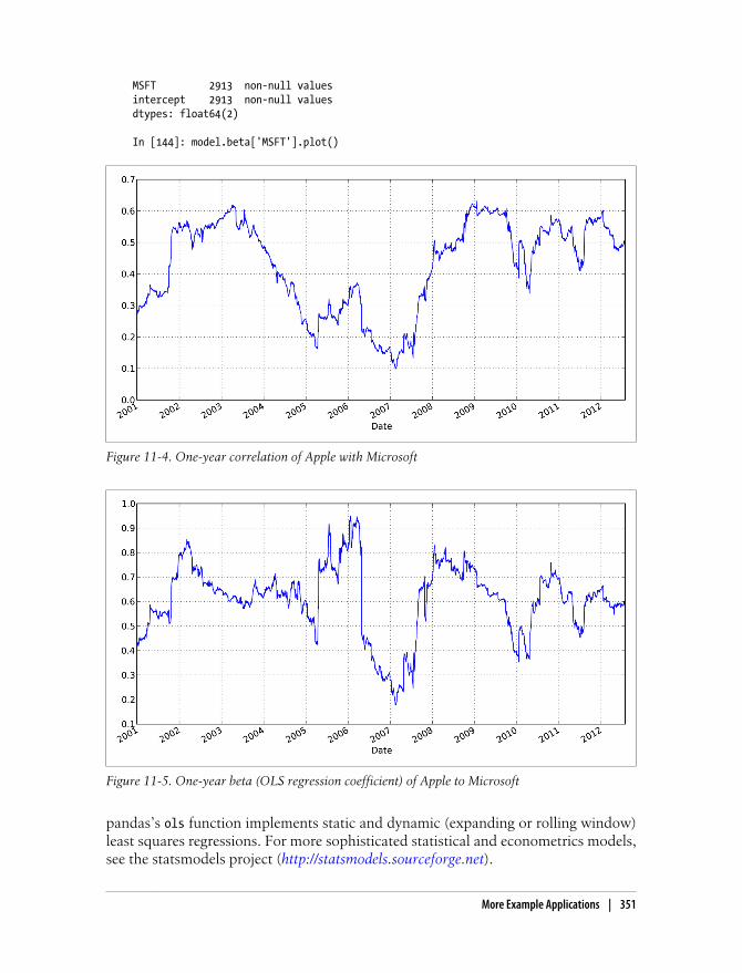
MSFT 2913 non-null valuesintercept 2913 non-null valuesdtypes: float64(2)
In [144]: model.beta['MSFT'].plot()
Figure 11-4. One-year correlation of Apple with Microsoft
Figure 11-5. One-year beta (OLS regression coefficient) of Apple to Microsoft
pandas’s ols function implements static and dynamic (expanding or rolling window)least squares regressions. For more sophisticated statistical and econometrics models,see the statsmodels project (http://statsmodels.sourceforge.net).
More Example Applications | 351


CHAPTER 12
Advanced NumPy
ndarray Object InternalsThe NumPy ndarray provides a means to interpret a block of homogeneous data (eithercontiguous or strided, more on this later) as a multidimensional array object. As you’veseen, the data type, or dtype, determines how the data is interpreted as being floatingpoint, integer, boolean, or any of the other types we’ve been looking at.
Part of what makes ndarray powerful is that every array object is a strided view on ablock of data. You might wonder, for example, how the array view arr[::2, ::-1] doesnot copy any data. Simply put, the ndarray is more than just a chunk of memory anda dtype; it also has striding information which enables the array to move throughmemory with varying step sizes. More precisely, the ndarray internally consists of thefollowing:
• A pointer to data, that is a block of system memory
• The data type or dtype
• A tuple indicating the array’s shape; For example, a 10 by 5 array would have shape(10, 5)
In [8]: np.ones((10, 5)).shapeOut[8]: (10, 5)
• A tuple of strides, integers indicating the number of bytes to “step” in order toadvance one element along a dimension; For example, a typical (C order, more onthis later) 3 x 4 x 5 array of float64 (8-byte) values has strides (160, 40, 8)
In [9]: np.ones((3, 4, 5), dtype=np.float64).stridesOut[9]: (160, 40, 8)
While it is rare that a typical NumPy user would be interested in the array strides,they are the critical ingredient in constructing copyless array views. Strides caneven be negative which enables an array to move backward through memory, whichwould be the case in a slice like obj[::-1] or obj[:, ::-1].
353

See Figure 12-1 for a simple mockup the ndarray innards.
Figure 12-1. The NumPy ndarray object
NumPy dtype HierarchyYou may occasionally have code which needs to check whether an array contains in-tegers, floating point numbers, strings, or Python objects. Because there are many typesof floating point numbers (float16 through float128), checking that the dtype is amonga list of types would be very verbose. Fortunately, the dtypes have superclasses such asnp.integer and np.floating which can be used in conjunction with the np.issubdtype function:
In [10]: ints = np.ones(10, dtype=np.uint16)
In [11]: floats = np.ones(10, dtype=np.float32)
In [12]: np.issubdtype(ints.dtype, np.integer)Out[12]: True
In [13]: np.issubdtype(floats.dtype, np.floating)Out[13]: True
You can see all of the parent classes of a specific dtype by calling the type’s mro method:
In [14]: np.float64.mro()Out[14]: [numpy.float64, numpy.floating, numpy.inexact, numpy.number, numpy.generic, float, object]
Most NumPy users will never have to know about this, but it occasionally comes inhandy. See Figure 12-2 for a graph of the dtype hierarchy and parent-subclassrelationships 1.
1. Some of the dtypes have trailing underscores in their names. These are there to avoid variable nameconflicts between the NumPy-specific types and the Python built-in ones.
354 | Chapter 12: Advanced NumPy

Advanced Array ManipulationThere are many ways to work with arrays beyond fancy indexing, slicing, and booleansubsetting. While much of the heavy lifting for data analysis applications is handled byhigher level functions in pandas, you may at some point need to write a data algorithmthat is not found in one of the existing libraries.
Reshaping ArraysGiven what we know about NumPy arrays, it should come as little surprise that youcan convert an array from one shape to another without copying any data. To do this,pass a tuple indicating the new shape to the reshape array instance method. For exam-ple, suppose we had a one-dimensional array of values that we wished to rearrange intoa matrix:
In [15]: arr = np.arange(8)
In [16]: arrOut[16]: array([0, 1, 2, 3, 4, 5, 6, 7])
In [17]: arr.reshape((4, 2))Out[17]: array([[0, 1], [2, 3], [4, 5], [6, 7]])
A multidimensional array can also be reshaped:
In [18]: arr.reshape((4, 2)).reshape((2, 4))Out[18]:
Figure 12-2. The NumPy dtype class hierarchy
Advanced Array Manipulation | 355

array([[0, 1, 2, 3], [4, 5, 6, 7]])
One of the passed shape dimensions can be -1, in which case the value used for thatdimension will be inferred from the data:
In [19]: arr = np.arange(15) In [20]: arr.reshape((5, -1)) Out[20]: array([[ 0, 1, 2], [ 3, 4, 5], [ 6, 7, 8], [ 9, 10, 11], [12, 13, 14]])
Since an array’s shape attribute is a tuple, it can be passed to reshape, too:
In [21]: other_arr = np.ones((3, 5))
In [22]: other_arr.shapeOut[22]: (3, 5)
In [23]: arr.reshape(other_arr.shape)Out[23]: array([[ 0, 1, 2, 3, 4], [ 5, 6, 7, 8, 9], [10, 11, 12, 13, 14]])
The opposite operation of reshape from one-dimensional to a higher dimension is typ-ically known as flattening or raveling:
In [24]: arr = np.arange(15).reshape((5, 3)) In [25]: arr Out[25]: array([[ 0, 1, 2], [ 3, 4, 5], [ 6, 7, 8], [ 9, 10, 11], [12, 13, 14]]) In [26]: arr.ravel()Out[26]: array([ 0, 1, 2, 3, 4, 5, 6, 7, 8, 9, 10, 11, 12, 13, 14])
ravel does not produce a copy of the underlying data if it does not have to (more onthis below). The flatten method behaves like ravel except it always returns a copy ofthe data:
In [27]: arr.flatten()Out[27]: array([ 0, 1, 2, 3, 4, 5, 6, 7, 8, 9, 10, 11, 12, 13, 14])
The data can be reshaped or raveled in different orders. This is a slightly nuanced topicfor new NumPy users and is therefore the next subtopic.
C versus Fortran OrderContrary to some other scientific computing environments like R and MATLAB,NumPy gives you much more control and flexibility over the layout of your data in
356 | Chapter 12: Advanced NumPy
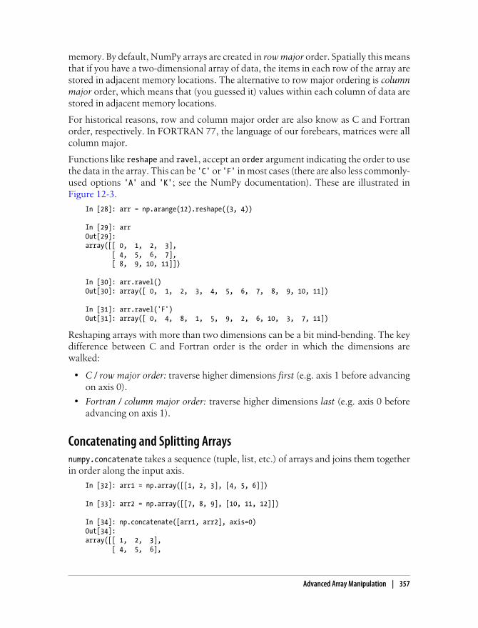
memory. By default, NumPy arrays are created in row major order. Spatially this meansthat if you have a two-dimensional array of data, the items in each row of the array arestored in adjacent memory locations. The alternative to row major ordering is columnmajor order, which means that (you guessed it) values within each column of data arestored in adjacent memory locations.
For historical reasons, row and column major order are also know as C and Fortranorder, respectively. In FORTRAN 77, the language of our forebears, matrices were allcolumn major.
Functions like reshape and ravel, accept an order argument indicating the order to usethe data in the array. This can be 'C' or 'F' in most cases (there are also less commonly-used options 'A' and 'K'; see the NumPy documentation). These are illustrated inFigure 12-3.
In [28]: arr = np.arange(12).reshape((3, 4))
In [29]: arrOut[29]: array([[ 0, 1, 2, 3], [ 4, 5, 6, 7], [ 8, 9, 10, 11]])
In [30]: arr.ravel()Out[30]: array([ 0, 1, 2, 3, 4, 5, 6, 7, 8, 9, 10, 11])
In [31]: arr.ravel('F')Out[31]: array([ 0, 4, 8, 1, 5, 9, 2, 6, 10, 3, 7, 11])
Reshaping arrays with more than two dimensions can be a bit mind-bending. The keydifference between C and Fortran order is the order in which the dimensions arewalked:
• C / row major order: traverse higher dimensions first (e.g. axis 1 before advancingon axis 0).
• Fortran / column major order: traverse higher dimensions last (e.g. axis 0 beforeadvancing on axis 1).
Concatenating and Splitting Arraysnumpy.concatenate takes a sequence (tuple, list, etc.) of arrays and joins them togetherin order along the input axis.
In [32]: arr1 = np.array([[1, 2, 3], [4, 5, 6]])
In [33]: arr2 = np.array([[7, 8, 9], [10, 11, 12]])
In [34]: np.concatenate([arr1, arr2], axis=0)Out[34]: array([[ 1, 2, 3], [ 4, 5, 6],
Advanced Array Manipulation | 357

[ 7, 8, 9], [10, 11, 12]])
In [35]: np.concatenate([arr1, arr2], axis=1)Out[35]: array([[ 1, 2, 3, 7, 8, 9], [ 4, 5, 6, 10, 11, 12]])
Figure 12-3. Reshaping in C (row major) or Fortran (column major) order
There are some convenience functions, like vstack and hstack, for common kinds ofconcatenation. The above operations could have been expressed as:
In [36]: np.vstack((arr1, arr2)) In [37]: np.hstack((arr1, arr2)) Out[36]: Out[37]: array([[ 1, 2, 3], array([[ 1, 2, 3, 7, 8, 9], [ 4, 5, 6], [ 4, 5, 6, 10, 11, 12]]) [ 7, 8, 9], [10, 11, 12]])
split, on the other hand, slices apart an array into multiple arrays along an axis:
In [38]: from numpy.random import randn
In [39]: arr = randn(5, 2) In [40]: arr Out[40]: array([[ 0.1689, 0.3287], [ 0.4703, 0.8989], [ 0.1535, 0.0243], [-0.2832, 1.1536], [ 0.2707, 0.8075]]) In [41]: first, second, third = np.split(arr, [1, 3])
In [42]: first
358 | Chapter 12: Advanced NumPy

Out[42]: array([[ 0.1689, 0.3287]])
In [43]: second In [44]: third Out[43]: Out[44]: array([[ 0.4703, 0.8989], array([[-0.2832, 1.1536], [ 0.1535, 0.0243]]) [ 0.2707, 0.8075]])
See Table 12-1 for a list of all relevant concatenation and splitting functions, some ofwhich are provided only as a convenience of the very general purpose concatenate.
Table 12-1. Array concatenation functions
Function Description
concatenate Most general function, concatenates collection of arrays along one axis
vstack, row_stack Stack arrays row-wise (along axis 0)
hstack Stack arrays column-wise (along axis 1)
column_stack Like hstack, but converts 1D arrays to 2D column vectors first
dstack Stack arrays “depth"-wise (along axis 2)
split Split array at passed locations along a particular axis
hsplit / vsplit / dsplit Convenience functions for splitting on axis 0, 1, and 2, respectively.
Stacking helpers: r_ and c_
There are two special objects in the NumPy namespace, r_ and c_, that make stackingarrays more concise:
In [45]: arr = np.arange(6)
In [46]: arr1 = arr.reshape((3, 2))
In [47]: arr2 = randn(3, 2)
In [48]: np.r_[arr1, arr2] In [49]: np.c_[np.r_[arr1, arr2], arr]Out[48]: Out[49]: array([[ 0. , 1. ], array([[ 0. , 1. , 0. ], [ 2. , 3. ], [ 2. , 3. , 1. ], [ 4. , 5. ], [ 4. , 5. , 2. ], [ 0.7258, -1.5325], [ 0.7258, -1.5325, 3. ], [-0.4696, -0.2127], [-0.4696, -0.2127, 4. ], [-0.1072, 1.2871]]) [-0.1072, 1.2871, 5. ]])
These additionally can translate slices to arrays:
In [50]: np.c_[1:6, -10:-5]Out[50]: array([[ 1, -10], [ 2, -9], [ 3, -8], [ 4, -7], [ 5, -6]])
See the docstring for more on what you can do with c_ and r_.
Advanced Array Manipulation | 359
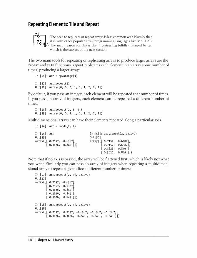
Repeating Elements: Tile and Repeat
The need to replicate or repeat arrays is less common with NumPy thanit is with other popular array programming languages like MATLAB.The main reason for this is that broadcasting fulfills this need better,which is the subject of the next section.
The two main tools for repeating or replicating arrays to produce larger arrays are the repeat and tile functions. repeat replicates each element in an array some number oftimes, producing a larger array:
In [51]: arr = np.arange(3)
In [52]: arr.repeat(3)Out[52]: array([0, 0, 0, 1, 1, 1, 2, 2, 2])
By default, if you pass an integer, each element will be repeated that number of times.If you pass an array of integers, each element can be repeated a different number oftimes:
In [53]: arr.repeat([2, 3, 4])Out[53]: array([0, 0, 1, 1, 1, 2, 2, 2, 2])
Multidimensional arrays can have their elements repeated along a particular axis.
In [54]: arr = randn(2, 2)
In [55]: arr In [56]: arr.repeat(2, axis=0)Out[55]: Out[56]: array([[ 0.7157, -0.6387], array([[ 0.7157, -0.6387], [ 0.3626, 0.849 ]]) [ 0.7157, -0.6387], [ 0.3626, 0.849 ], [ 0.3626, 0.849 ]])
Note that if no axis is passed, the array will be flattened first, which is likely not whatyou want. Similarly you can pass an array of integers when repeating a multidimen-sional array to repeat a given slice a different number of times:
In [57]: arr.repeat([2, 3], axis=0)Out[57]: array([[ 0.7157, -0.6387], [ 0.7157, -0.6387], [ 0.3626, 0.849 ], [ 0.3626, 0.849 ], [ 0.3626, 0.849 ]])
In [58]: arr.repeat([2, 3], axis=1)Out[58]: array([[ 0.7157, 0.7157, -0.6387, -0.6387, -0.6387], [ 0.3626, 0.3626, 0.849 , 0.849 , 0.849 ]])
360 | Chapter 12: Advanced NumPy

tile, on the other hand, is a shortcut for stacking copies of an array along an axis. Youcan visually think about it as like “laying down tiles”:
In [59]: arrOut[59]: array([[ 0.7157, -0.6387], [ 0.3626, 0.849 ]])
In [60]: np.tile(arr, 2)Out[60]: array([[ 0.7157, -0.6387, 0.7157, -0.6387], [ 0.3626, 0.849 , 0.3626, 0.849 ]])
The second argument is the number of tiles; with a scalar, the tiling is made row-by-row, rather than column by column: The second argument to tile can be a tuple in-dicating the layout of the “tiling”:
In [61]: arrOut[61]: array([[ 0.7157, -0.6387], [ 0.3626, 0.849 ]])
In [62]: np.tile(arr, (2, 1)) In [63]: np.tile(arr, (3, 2)) Out[62]: Out[63]: array([[ 0.7157, -0.6387], array([[ 0.7157, -0.6387, 0.7157, -0.6387], [ 0.3626, 0.849 ], [ 0.3626, 0.849 , 0.3626, 0.849 ], [ 0.7157, -0.6387], [ 0.7157, -0.6387, 0.7157, -0.6387], [ 0.3626, 0.849 ]]) [ 0.3626, 0.849 , 0.3626, 0.849 ], [ 0.7157, -0.6387, 0.7157, -0.6387], [ 0.3626, 0.849 , 0.3626, 0.849 ]])
Fancy Indexing Equivalents: Take and PutAs you may recall from Chapter 4, one way to get and set subsets of arrays is by fancy indexing using integer arrays:
In [64]: arr = np.arange(10) * 100
In [65]: inds = [7, 1, 2, 6] In [66]: arr[inds] Out[66]: array([700, 100, 200, 600])
There are alternate ndarray methods that are useful in the special case of only makinga selection on a single axis:
In [67]: arr.take(inds)Out[67]: array([700, 100, 200, 600])
In [68]: arr.put(inds, 42)
In [69]: arrOut[69]: array([ 0, 42, 42, 300, 400, 500, 42, 42, 800, 900])
In [70]: arr.put(inds, [40, 41, 42, 43])
Advanced Array Manipulation | 361
In [71]: arrOut[71]: array([ 0, 41, 42, 300, 400, 500, 43, 40, 800, 900])
To use take along other axes, you can pass the axis keyword:
In [72]: inds = [2, 0, 2, 1]
In [73]: arr = randn(2, 4)
In [74]: arrOut[74]: array([[-0.8237, 2.6047, -0.4578, -1. ], [ 2.3198, -1.0792, 0.518 , 0.2527]])
In [75]: arr.take(inds, axis=1)Out[75]: array([[-0.4578, -0.8237, -0.4578, 2.6047], [ 0.518 , 2.3198, 0.518 , -1.0792]])
put does not accept an axis argument but rather indexes into the flattened (one-di-mensional, C order) version of the array (this could be changed in principle). Thus,when you need to set elements using an index array on other axes, you will want to usefancy indexing.
As of this writing, the take and put functions in general have betterperformance than their fancy indexing equivalents by a significant mar-gin. I regard this as a “bug” and something to be fixed in NumPy, butit’s something worth keeping in mind if you’re selecting subsets of largearrays using integer arrays:
In [76]: arr = randn(1000, 50)
# Random sample of 500 rowsIn [77]: inds = np.random.permutation(1000)[:500]
In [78]: %timeit arr[inds]1000 loops, best of 3: 356 us per loop
In [79]: %timeit arr.take(inds, axis=0)10000 loops, best of 3: 34 us per loop
BroadcastingBroadcasting describes how arithmetic works between arrays of different shapes. It isa very powerful feature, but one that can be easily misunderstood, even by experiencedusers. The simplest example of broadcasting occurs when combining a scalar valuewith an array:
In [80]: arr = np.arange(5)
In [81]: arr In [82]: arr * 4 Out[81]: array([0, 1, 2, 3, 4]) Out[82]: array([ 0, 4, 8, 12, 16])
362 | Chapter 12: Advanced NumPy
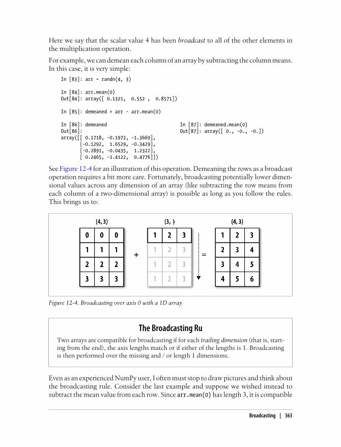
Here we say that the scalar value 4 has been broadcast to all of the other elements inthe multiplication operation.
For example, we can demean each column of an array by subtracting the column means.In this case, it is very simple:
In [83]: arr = randn(4, 3)
In [84]: arr.mean(0)Out[84]: array([ 0.1321, 0.552 , 0.8571])
In [85]: demeaned = arr - arr.mean(0)
In [86]: demeaned In [87]: demeaned.mean(0) Out[86]: Out[87]: array([ 0., -0., -0.])array([[ 0.1718, -0.1972, -1.3669], [-0.1292, 1.6529, -0.3429], [-0.2891, -0.0435, 1.2322], [ 0.2465, -1.4122, 0.4776]])
See Figure 12-4 for an illustration of this operation. Demeaning the rows as a broadcastoperation requires a bit more care. Fortunately, broadcasting potentially lower dimen-sional values across any dimension of an array (like subtracting the row means fromeach column of a two-dimensional array) is possible as long as you follow the rules.This brings us to:
Figure 12-4. Broadcasting over axis 0 with a 1D array
The Broadcasting RuTwo arrays are compatible for broadcasting if for each trailing dimension (that is, start-ing from the end), the axis lengths match or if either of the lengths is 1. Broadcastingis then performed over the missing and / or length 1 dimensions.
Even as an experienced NumPy user, I often must stop to draw pictures and think aboutthe broadcasting rule. Consider the last example and suppose we wished instead tosubtract the mean value from each row. Since arr.mean(0) has length 3, it is compatible
Broadcasting | 363

for broadcasting across axis 0 because the trailing dimension in arr is 3 and thereforematches. According to the rules, to subtract over axis 1 (that is, subtract the row meanfrom each row), the smaller array must have shape (4, 1):
In [88]: arrOut[88]: array([[ 0.3039, 0.3548, -0.5097], [ 0.0029, 2.2049, 0.5142], [-0.1571, 0.5085, 2.0893], [ 0.3786, -0.8602, 1.3347]])
In [89]: row_means = arr.mean(1) In [90]: row_means.reshape((4, 1)) Out[90]: array([[ 0.0496], [ 0.9073], [ 0.8136], [ 0.2844]]) In [91]: demeaned = arr - row_means.reshape((4, 1))
In [92]: demeaned.mean(1)Out[92]: array([ 0., 0., 0., 0.])
Has your head exploded yet? See Figure 12-5 for an illustration of this operation.
Figure 12-5. Broadcasting over axis 1 of a 2D array
See Figure 12-6 for another illustration, this time subtracting a two-dimensional arrayfrom a three-dimensional one across axis 0.
Broadcasting Over Other AxesBroadcasting with higher dimensional arrays can seem even more mind-bending, butit is really a matter of following the rules. If you don’t, you’ll get an error like this:
In [93]: arr - arr.mean(1)---------------------------------------------------------------------------ValueError Traceback (most recent call last)<ipython-input-93-7b87b85a20b2> in <module>()
364 | Chapter 12: Advanced NumPy

----> 1 arr - arr.mean(1)ValueError: operands could not be broadcast together with shapes (4,3) (4)
Figure 12-6. Broadcasting over axis 0 of a 3D array
It’s quite common to want to perform an arithmetic operation with a lower dimensionalarray across axes other than axis 0. According to the broadcasting rule, the “broadcastdimensions” must be 1 in the smaller array. In the example of row demeaning abovethis meant reshaping the row means to be shape (4, 1) instead of (4,):
In [94]: arr - arr.mean(1).reshape((4, 1))Out[94]: array([[ 0.2542, 0.3051, -0.5594], [-0.9044, 1.2976, -0.3931], [-0.9707, -0.3051, 1.2757], [ 0.0942, -1.1446, 1.0503]])
In the three-dimensional case, broadcasting over any of the three dimensions is only amatter of reshaping the data to be shape-compatible. See Figure 12-7 for a nice visual-ization of the shapes required to broadcast over each axis of a three-dimensional array.
A very common problem, therefore, is needing to add a new axis with length 1 specif-ically for broadcasting purposes, especially in generic algorithms. Using reshape is oneoption, but inserting an axis requires constructing a tuple indicating the new shape.This can often be a tedious exercise. Thus, NumPy arrays offer a special syntax forinserting new axes by indexing. We use the special np.newaxis attribute along with“full” slices to insert the new axis:
In [95]: arr = np.zeros((4, 4))
In [96]: arr_3d = arr[:, np.newaxis, :] In [97]: arr_3d.shape Out[97]: (4, 1, 4)
In [98]: arr_1d = np.random.normal(size=3)
In [99]: arr_1d[:, np.newaxis] In [100]: arr_1d[np.newaxis, :] Out[99]: Out[100]: array([[-0.3899, 0.396 , -0.1852]])
Broadcasting | 365

array([[-0.3899], [ 0.396 ], [-0.1852]])
Figure 12-7. Compatible 2D array shapes for broadcasting over a 3D array
Thus, if we had a three-dimensional array and wanted to demean axis 2, say, we wouldonly need to write:
In [101]: arr = randn(3, 4, 5)
In [102]: depth_means = arr.mean(2)
In [103]: depth_meansOut[103]: array([[ 0.1097, 0.3118, -0.5473, 0.2663], [ 0.1747, 0.1379, 0.1146, -0.4224], [ 0.0217, 0.3686, -0.0468, 1.3026]])
In [104]: demeaned = arr - depth_means[:, :, np.newaxis]
In [105]: demeaned.mean(2)Out[105]: array([[ 0., 0., -0., 0.], [ 0., -0., -0., 0.], [-0., -0., 0., 0.]])
If you’re completely confused by this, don’t worry. With practice you will get the hangof it!
366 | Chapter 12: Advanced NumPy

Some readers might wonder if there’s a way to generalize demeaning over an axiswithout sacrificing performance. There is, in fact, but it requires some indexinggymnastics:
def demean_axis(arr, axis=0): means = arr.mean(axis)
# This generalized things like [:, :, np.newaxis] to N dimensions indexer = [slice(None)] * arr.ndim indexer[axis] = np.newaxis return arr - means[indexer]
Setting Array Values by BroadcastingThe same broadcasting rule governing arithmetic operations also applies to settingvalues via array indexing. In the simplest case, we can do things like:
In [106]: arr = np.zeros((4, 3))
In [107]: arr[:] = 5 In [108]: arr Out[108]: array([[ 5., 5., 5.], [ 5., 5., 5.], [ 5., 5., 5.], [ 5., 5., 5.]])
However, if we had a one-dimensional array of values we wanted to set into the columnsof the array, we can do that as long as the shape is compatible:
In [109]: col = np.array([1.28, -0.42, 0.44, 1.6])
In [110]: arr[:] = col[:, np.newaxis] In [111]: arr Out[111]: array([[ 1.28, 1.28, 1.28], [-0.42, -0.42, -0.42], [ 0.44, 0.44, 0.44], [ 1.6 , 1.6 , 1.6 ]]) In [112]: arr[:2] = [[-1.37], [0.509]] In [113]: arr Out[113]: array([[-1.37 , -1.37 , -1.37 ], [ 0.509, 0.509, 0.509], [ 0.44 , 0.44 , 0.44 ], [ 1.6 , 1.6 , 1.6 ]])
Advanced ufunc UsageWhile many NumPy users will only make use of the fast element-wise operations pro-vided by the universal functions, there are a number of additional features that occa-sionally can help you write more concise code without loops.
Advanced ufunc Usage | 367

ufunc Instance MethodsEach of NumPy’s binary ufuncs has special methods for performing certain kinds ofspecial vectorized operations. These are summarized in Table 12-2, but I’ll give a fewconcrete examples to illustrate how they work.
reduce takes a single array and aggregates its values, optionally along an axis, by per-forming a sequence of binary operations. For example, an alternate way to sum ele-ments in an array is to use np.add.reduce:
In [114]: arr = np.arange(10)
In [115]: np.add.reduce(arr)Out[115]: 45
In [116]: arr.sum()Out[116]: 45
The starting value (0 for add) depends on the ufunc. If an axis is passed, the reductionis performed along that axis. This allows you to answer certain kinds of questions in aconcise way. As a less trivial example, we can use np.logical_and to check whether thevalues in each row of an array are sorted:
In [118]: arr = randn(5, 5)
In [119]: arr[::2].sort(1) # sort a few rows
In [120]: arr[:, :-1] < arr[:, 1:]Out[120]: array([[ True, True, True, True], [False, True, False, False], [ True, True, True, True], [ True, False, True, True], [ True, True, True, True]], dtype=bool)
In [121]: np.logical_and.reduce(arr[:, :-1] < arr[:, 1:], axis=1)Out[121]: array([ True, False, True, False, True], dtype=bool)
Of course, logical_and.reduce is equivalent to the all method.
accumulate is related to reduce like cumsum is related to sum. It produces an array of thesame size with the intermediate “accumulated” values:
In [122]: arr = np.arange(15).reshape((3, 5))
In [123]: np.add.accumulate(arr, axis=1)Out[123]: array([[ 0, 1, 3, 6, 10], [ 5, 11, 18, 26, 35], [10, 21, 33, 46, 60]])
outer performs a pairwise cross-product between two arrays:
In [124]: arr = np.arange(3).repeat([1, 2, 2])
368 | Chapter 12: Advanced NumPy

In [125]: arrOut[125]: array([0, 1, 1, 2, 2])
In [126]: np.multiply.outer(arr, np.arange(5))Out[126]: array([[0, 0, 0, 0, 0], [0, 1, 2, 3, 4], [0, 1, 2, 3, 4], [0, 2, 4, 6, 8], [0, 2, 4, 6, 8]])
The output of outer will have a dimension that is the sum of the dimensions of theinputs:
In [127]: result = np.subtract.outer(randn(3, 4), randn(5))
In [128]: result.shapeOut[128]: (3, 4, 5)
The last method, reduceat, performs a “local reduce”, in essence an array groupby op-eration in which slices of the array are aggregated together. While it’s less flexible thanthe GroupBy capabilities in pandas, it can be very fast and powerful in the right cir-cumstances. It accepts a sequence of “bin edges” which indicate how to split and ag-gregate the values:
In [129]: arr = np.arange(10)
In [130]: np.add.reduceat(arr, [0, 5, 8])Out[130]: array([10, 18, 17])
The results are the reductions (here, sums) performed over arr[0:5], arr[5:8], andarr[8:]. Like the other methods, you can pass an axis argument:
In [131]: arr = np.multiply.outer(np.arange(4), np.arange(5))
In [132]: arr In [133]: np.add.reduceat(arr, [0, 2, 4], axis=1)Out[132]: Out[133]: array([[ 0, 0, 0, 0, 0], array([[ 0, 0, 0], [ 0, 1, 2, 3, 4], [ 1, 5, 4], [ 0, 2, 4, 6, 8], [ 2, 10, 8], [ 0, 3, 6, 9, 12]]) [ 3, 15, 12]])
Table 12-2. ufunc methods
Method Description
reduce(x) Aggregate values by successive applications of the operation
accumulate(x) Aggregate values, preserving all partial aggregates
reduceat(x, bins) “Local” reduce or “group by”. Reduce contiguous slices of data to produce aggregatedarray.
outer(x, y) Apply operation to all pairs of elements in x and y. Result array has shape x.shape +y.shape
Advanced ufunc Usage | 369

Custom ufuncsThere are a couple facilities for creating your own functions with ufunc-like semantics. numpy.frompyfunc accepts a Python function along with a specification for the numberof inputs and outputs. For example, a simple function that adds element-wise wouldbe specified as:
In [134]: def add_elements(x, y): .....: return x + y
In [135]: add_them = np.frompyfunc(add_elements, 2, 1)
In [136]: add_them(np.arange(8), np.arange(8))Out[136]: array([0, 2, 4, 6, 8, 10, 12, 14], dtype=object)
Functions created using frompyfunc always return arrays of Python objects which isn’tvery convenient. Fortunately, there is an alternate, but slightly less featureful function numpy.vectorize that is a bit more intelligent about type inference:
In [137]: add_them = np.vectorize(add_elements, otypes=[np.float64])
In [138]: add_them(np.arange(8), np.arange(8))Out[138]: array([ 0., 2., 4., 6., 8., 10., 12., 14.])
These functions provide a way to create ufunc-like functions, but they are very slowbecause they require a Python function call to compute each element, which is a lotslower than NumPy’s C-based ufunc loops:
In [139]: arr = randn(10000)
In [140]: %timeit add_them(arr, arr)100 loops, best of 3: 2.12 ms per loop
In [141]: %timeit np.add(arr, arr)100000 loops, best of 3: 11.6 us per loop
There are a number of projects under way in the scientific Python community to makeit easier to define new ufuncs whose performance is closer to that of the built-in ones.
Structured and Record ArraysYou may have noticed up until now that ndarray is a homogeneous data container; thatis, it represents a block of memory in which each element takes up the same numberof bytes, determined by the dtype. On the surface, this would appear to not allow youto represent heterogeneous or tabular-like data. A structured array is an ndarray inwhich each element can be thought of as representing a struct in C (hence the “struc-tured” name) or a row in a SQL table with multiple named fields:
In [142]: dtype = [('x', np.float64), ('y', np.int32)]
In [143]: sarr = np.array([(1.5, 6), (np.pi, -2)], dtype=dtype)
370 | Chapter 12: Advanced NumPy

In [144]: sarrOut[144]: array([(1.5, 6), (3.141592653589793, -2)], dtype=[('x', '<f8'), ('y', '<i4')])
There are several ways to specify a structured dtype (see the online NumPy documen-tation). One typical way is as a list of tuples with (field_name, field_data_type). Now,the elements of the array are tuple-like objects whose elements can be accessed like adictionary:
In [145]: sarr[0]Out[145]: (1.5, 6)
In [146]: sarr[0]['y']Out[146]: 6
The field names are stored in the dtype.names attribute. On accessing a field on thestructured array, a strided view on the data is returned thus copying nothing:
In [147]: sarr['x']Out[147]: array([ 1.5 , 3.1416])
Nested dtypes and Multidimensional FieldsWhen specifying a structured dtype, you can additionally pass a shape (as an int ortuple):
In [148]: dtype = [('x', np.int64, 3), ('y', np.int32)]
In [149]: arr = np.zeros(4, dtype=dtype)
In [150]: arrOut[150]: array([([0, 0, 0], 0), ([0, 0, 0], 0), ([0, 0, 0], 0), ([0, 0, 0], 0)], dtype=[('x', '<i8', (3,)), ('y', '<i4')])
In this case, the x field now refers to an array of length three for each record:
In [151]: arr[0]['x']Out[151]: array([0, 0, 0])
Conveniently, accessing arr['x'] then returns a two-dimensional array instead of aone-dimensional array as in prior examples:
In [152]: arr['x']Out[152]: array([[0, 0, 0], [0, 0, 0], [0, 0, 0], [0, 0, 0]])
This enables you to express more complicated, nested structures as a single block ofmemory in an array. Though, since dtypes can be arbitrarily complex, why not nesteddtypes? Here is a simple example:
Structured and Record Arrays | 371

In [153]: dtype = [('x', [('a', 'f8'), ('b', 'f4')]), ('y', np.int32)]
In [154]: data = np.array([((1, 2), 5), ((3, 4), 6)], dtype=dtype)
In [155]: data['x']Out[155]: array([(1.0, 2.0), (3.0, 4.0)], dtype=[('a', '<f8'), ('b', '<f4')])
In [156]: data['y']Out[156]: array([5, 6], dtype=int32)
In [157]: data['x']['a']Out[157]: array([ 1., 3.])
As you can see, variable-shape fields and nested records is a very rich feature that canbe the right tool in certain circumstances. A DataFrame from pandas, by contrast, doesnot support this feature directly, though it is similar to hierarchical indexing.
Why Use Structured Arrays?Compared with, say, a DataFrame from pandas, NumPy structured arrays are a com-paratively low-level tool. They provide a means to interpreting a block of memory as atabular structure with arbitrarily complex nested columns. Since each element in thearray is represented in memory as a fixed number of bytes, structured arrays provide avery fast and efficient way of writing data to and from disk (including memory maps,more on this later), transporting it over the network, and other such use.
As another common use for structured arrays, writing data files as fixed length recordbyte streams is a common way to serialize data in C and C++ code, which is commonlyfound in legacy systems in industry. As long as the format of the file is known (the sizeof each record and the order, byte size, and data type of each element), the data can beread into memory using np.fromfile. Specialized uses like this are beyond the scope ofthis book, but it’s worth knowing that such things are possible.
Structured Array Manipulations: numpy.lib.recfunctionsWhile there is not as much functionality available for structured arrays as for Data-Frames, the NumPy module numpy.lib.recfunctions has some helpful tools for addingand dropping fields or doing basic join-like operations. The thing to remember withthese tools is that it is typically necessary to create a new array to make any modifica-tions to the dtype (like adding or dropping a column). These functions are left to theinterested reader to explore as I do not use them anywhere in this book.
372 | Chapter 12: Advanced NumPy

More About SortingLike Python’s built-in list, the ndarray sort instance method is an in-place sort, meaningthat the array contents are rearranged without producing a new array:
In [158]: arr = randn(6)
In [159]: arr.sort()
In [160]: arrOut[160]: array([-1.082 , 0.3759, 0.8014, 1.1397, 1.2888, 1.8413])
When sorting arrays in-place, remember that if the array is a view on a different ndarray,the original array will be modified:
In [161]: arr = randn(3, 5)
In [162]: arrOut[162]: array([[-0.3318, -1.4711, 0.8705, -0.0847, -1.1329], [-1.0111, -0.3436, 2.1714, 0.1234, -0.0189], [ 0.1773, 0.7424, 0.8548, 1.038 , -0.329 ]])
In [163]: arr[:, 0].sort() # Sort first column values in-place
In [164]: arrOut[164]: array([[-1.0111, -1.4711, 0.8705, -0.0847, -1.1329], [-0.3318, -0.3436, 2.1714, 0.1234, -0.0189], [ 0.1773, 0.7424, 0.8548, 1.038 , -0.329 ]])
On the other hand, numpy.sort creates a new, sorted copy of an array. Otherwise itaccepts the same arguments (such as kind, more on this below) as ndarray.sort:
In [165]: arr = randn(5)
In [166]: arrOut[166]: array([-1.1181, -0.2415, -2.0051, 0.7379, -1.0614])
In [167]: np.sort(arr)Out[167]: array([-2.0051, -1.1181, -1.0614, -0.2415, 0.7379])
In [168]: arrOut[168]: array([-1.1181, -0.2415, -2.0051, 0.7379, -1.0614])
All of these sort methods take an axis argument for sorting the sections of data alongthe passed axis independently:
In [169]: arr = randn(3, 5)
In [170]: arrOut[170]: array([[ 0.5955, -0.2682, 1.3389, -0.1872, 0.9111], [-0.3215, 1.0054, -0.5168, 1.1925, -0.1989], [ 0.3969, -1.7638, 0.6071, -0.2222, -0.2171]])
More About Sorting | 373
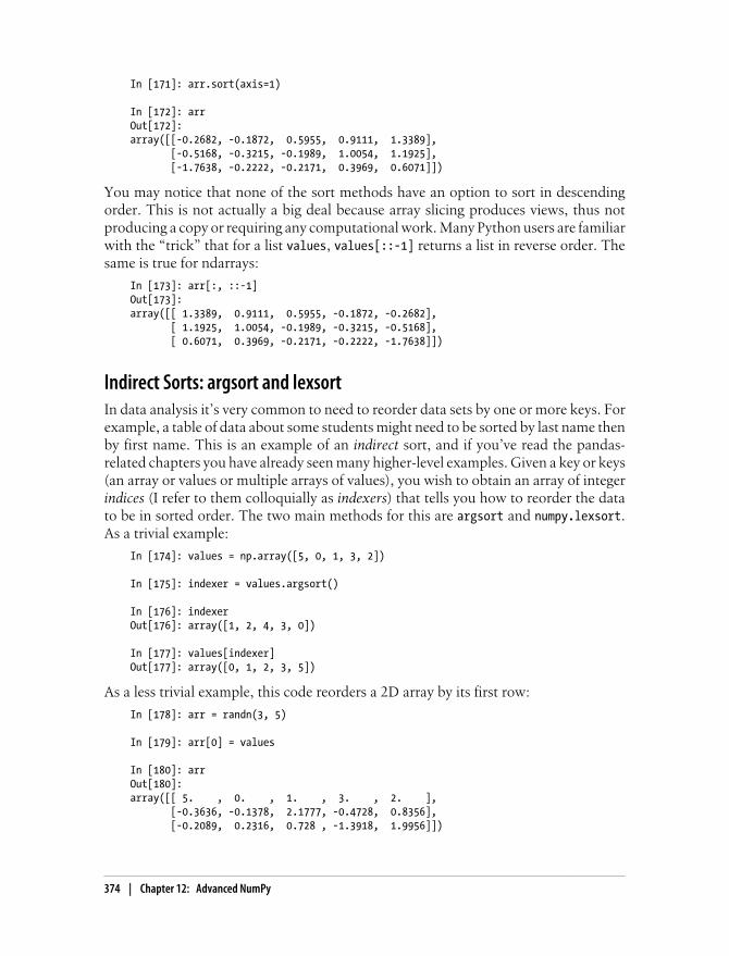
In [171]: arr.sort(axis=1)
In [172]: arrOut[172]: array([[-0.2682, -0.1872, 0.5955, 0.9111, 1.3389], [-0.5168, -0.3215, -0.1989, 1.0054, 1.1925], [-1.7638, -0.2222, -0.2171, 0.3969, 0.6071]])
You may notice that none of the sort methods have an option to sort in descendingorder. This is not actually a big deal because array slicing produces views, thus notproducing a copy or requiring any computational work. Many Python users are familiarwith the “trick” that for a list values, values[::-1] returns a list in reverse order. Thesame is true for ndarrays:
In [173]: arr[:, ::-1]Out[173]: array([[ 1.3389, 0.9111, 0.5955, -0.1872, -0.2682], [ 1.1925, 1.0054, -0.1989, -0.3215, -0.5168], [ 0.6071, 0.3969, -0.2171, -0.2222, -1.7638]])
Indirect Sorts: argsort and lexsortIn data analysis it’s very common to need to reorder data sets by one or more keys. Forexample, a table of data about some students might need to be sorted by last name thenby first name. This is an example of an indirect sort, and if you’ve read the pandas-related chapters you have already seen many higher-level examples. Given a key or keys(an array or values or multiple arrays of values), you wish to obtain an array of integerindices (I refer to them colloquially as indexers) that tells you how to reorder the datato be in sorted order. The two main methods for this are argsort and numpy.lexsort.As a trivial example:
In [174]: values = np.array([5, 0, 1, 3, 2])
In [175]: indexer = values.argsort()
In [176]: indexerOut[176]: array([1, 2, 4, 3, 0])
In [177]: values[indexer]Out[177]: array([0, 1, 2, 3, 5])
As a less trivial example, this code reorders a 2D array by its first row:
In [178]: arr = randn(3, 5)
In [179]: arr[0] = values
In [180]: arrOut[180]: array([[ 5. , 0. , 1. , 3. , 2. ], [-0.3636, -0.1378, 2.1777, -0.4728, 0.8356], [-0.2089, 0.2316, 0.728 , -1.3918, 1.9956]])
374 | Chapter 12: Advanced NumPy

In [181]: arr[:, arr[0].argsort()]Out[181]: array([[ 0. , 1. , 2. , 3. , 5. ], [-0.1378, 2.1777, 0.8356, -0.4728, -0.3636], [ 0.2316, 0.728 , 1.9956, -1.3918, -0.2089]])
lexsort is similar to argsort, but it performs an indirect lexicographical sort on multiplekey arrays. Suppose we wanted to sort some data identified by first and last names:
In [182]: first_name = np.array(['Bob', 'Jane', 'Steve', 'Bill', 'Barbara'])
In [183]: last_name = np.array(['Jones', 'Arnold', 'Arnold', 'Jones', 'Walters'])
In [184]: sorter = np.lexsort((first_name, last_name))
In [185]: zip(last_name[sorter], first_name[sorter])Out[185]: [('Arnold', 'Jane'), ('Arnold', 'Steve'), ('Jones', 'Bill'), ('Jones', 'Bob'), ('Walters', 'Barbara')]
lexsort can be a bit confusing the first time you use it because the order in which thekeys are used to order the data starts with the last array passed. As you can see,last_name was used before first_name.
pandas methods like Series’s and DataFrame’s sort_index methods andthe Series order method are implemented with variants of these func-tions (which also must take into account missing values)
Alternate Sort AlgorithmsA stable sorting algorithm preserves the relative position of equal elements. This canbe especially important in indirect sorts where the relative ordering is meaningful:
In [186]: values = np.array(['2:first', '2:second', '1:first', '1:second', '1:third'])
In [187]: key = np.array([2, 2, 1, 1, 1])
In [188]: indexer = key.argsort(kind='mergesort')
In [189]: indexerOut[189]: array([2, 3, 4, 0, 1])
In [190]: values.take(indexer)Out[190]: array(['1:first', '1:second', '1:third', '2:first', '2:second'], dtype='|S8')
The only stable sort available is mergesort which has guaranteed O(n log n) performance(for complexity buffs), but its performance is on average worse than the default
More About Sorting | 375

quicksort method. See Table 12-3 for a summary of available methods and their relativeperformance (and performance guarantees). This is not something that most users willever have to think about but useful to know that it’s there.
Table 12-3. Array sorting methods
Kind Speed Stable Work space Worst-case
'quicksort' 1 No 0 O(n2)
'mergesort' 2 Yes n / 2 O(n log n)
'heapsort' 3 No 0 O(n log n)
At the time of this writing, sort algorithms other than quicksort are notavailable on arrays of Python objects (dtype=object). This means occa-sionally that algorithms requiring stable sorting will require work-arounds when dealing with Python objects.
numpy.searchsorted: Finding elements in a Sorted Arraysearchsorted is an array method that performs a binary search on a sorted array, re-turning the location in the array where the value would need to be inserted to maintainsortedness:
In [191]: arr = np.array([0, 1, 7, 12, 15])
In [192]: arr.searchsorted(9)Out[192]: 3
As you might expect, you can also pass an array of values to get an array of indices back:
In [193]: arr.searchsorted([0, 8, 11, 16])Out[193]: array([0, 3, 3, 5])
You might have noticed that searchsorted returned 0 for the 0 element. This is becausethe default behavior is to return the index at the left side of a group of equal values:
In [194]: arr = np.array([0, 0, 0, 1, 1, 1, 1])
In [195]: arr.searchsorted([0, 1])Out[195]: array([0, 3])
In [196]: arr.searchsorted([0, 1], side='right')Out[196]: array([3, 7])
As another application of searchsorted, suppose we had an array of values between 0and 10,000) and a separate array of “bucket edges” that we wanted to use to bin thedata:
In [197]: data = np.floor(np.random.uniform(0, 10000, size=50))
In [198]: bins = np.array([0, 100, 1000, 5000, 10000])
In [199]: data
376 | Chapter 12: Advanced NumPy
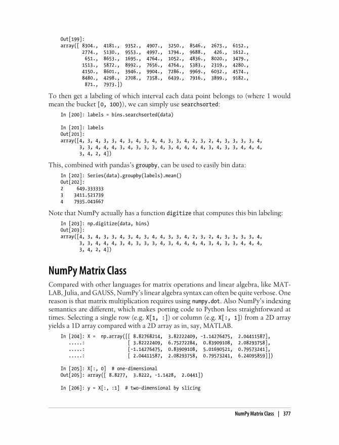
Out[199]: array([ 8304., 4181., 9352., 4907., 3250., 8546., 2673., 6152., 2774., 5130., 9553., 4997., 1794., 9688., 426., 1612., 651., 8653., 1695., 4764., 1052., 4836., 8020., 3479., 1513., 5872., 8992., 7656., 4764., 5383., 2319., 4280., 4150., 8601., 3946., 9904., 7286., 9969., 6032., 4574., 8480., 4298., 2708., 7358., 6439., 7916., 3899., 9182., 871., 7973.])
To then get a labeling of which interval each data point belongs to (where 1 wouldmean the bucket [0, 100)), we can simply use searchsorted:
In [200]: labels = bins.searchsorted(data)
In [201]: labelsOut[201]: array([4, 3, 4, 3, 3, 4, 3, 4, 3, 4, 4, 3, 3, 4, 2, 3, 2, 4, 3, 3, 3, 3, 4, 3, 3, 4, 4, 4, 3, 4, 3, 3, 3, 4, 3, 4, 4, 4, 4, 3, 4, 3, 3, 4, 4, 4, 3, 4, 2, 4])
This, combined with pandas’s groupby, can be used to easily bin data:
In [202]: Series(data).groupby(labels).mean()Out[202]: 2 649.3333333 3411.5217394 7935.041667
Note that NumPy actually has a function digitize that computes this bin labeling:
In [203]: np.digitize(data, bins)Out[203]: array([4, 3, 4, 3, 3, 4, 3, 4, 3, 4, 4, 3, 3, 4, 2, 3, 2, 4, 3, 3, 3, 3, 4, 3, 3, 4, 4, 4, 3, 4, 3, 3, 3, 4, 3, 4, 4, 4, 4, 3, 4, 3, 3, 4, 4, 4, 3, 4, 2, 4])
NumPy Matrix ClassCompared with other languages for matrix operations and linear algebra, like MAT-LAB, Julia, and GAUSS, NumPy’s linear algebra syntax can often be quite verbose. Onereason is that matrix multiplication requires using numpy.dot. Also NumPy’s indexingsemantics are different, which makes porting code to Python less straightforward attimes. Selecting a single row (e.g. X[1, :]) or column (e.g. X[:, 1]) from a 2D arrayyields a 1D array compared with a 2D array as in, say, MATLAB.
In [204]: X = np.array([[ 8.82768214, 3.82222409, -1.14276475, 2.04411587], .....: [ 3.82222409, 6.75272284, 0.83909108, 2.08293758], .....: [-1.14276475, 0.83909108, 5.01690521, 0.79573241], .....: [ 2.04411587, 2.08293758, 0.79573241, 6.24095859]])
In [205]: X[:, 0] # one-dimensionalOut[205]: array([ 8.8277, 3.8222, -1.1428, 2.0441])
In [206]: y = X[:, :1] # two-dimensional by slicing
NumPy Matrix Class | 377
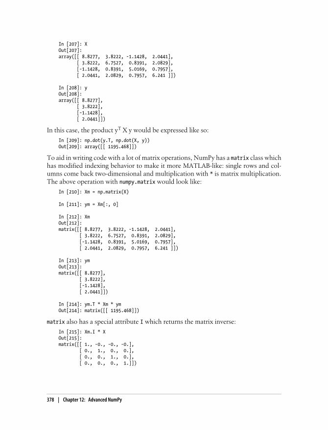
In [207]: XOut[207]: array([[ 8.8277, 3.8222, -1.1428, 2.0441], [ 3.8222, 6.7527, 0.8391, 2.0829], [-1.1428, 0.8391, 5.0169, 0.7957], [ 2.0441, 2.0829, 0.7957, 6.241 ]])
In [208]: yOut[208]: array([[ 8.8277], [ 3.8222], [-1.1428], [ 2.0441]])
In this case, the product yT X y would be expressed like so:
In [209]: np.dot(y.T, np.dot(X, y))Out[209]: array([[ 1195.468]])
To aid in writing code with a lot of matrix operations, NumPy has a matrix class whichhas modified indexing behavior to make it more MATLAB-like: single rows and col-umns come back two-dimensional and multiplication with * is matrix multiplication.The above operation with numpy.matrix would look like:
In [210]: Xm = np.matrix(X)
In [211]: ym = Xm[:, 0]
In [212]: XmOut[212]: matrix([[ 8.8277, 3.8222, -1.1428, 2.0441], [ 3.8222, 6.7527, 0.8391, 2.0829], [-1.1428, 0.8391, 5.0169, 0.7957], [ 2.0441, 2.0829, 0.7957, 6.241 ]])
In [213]: ymOut[213]: matrix([[ 8.8277], [ 3.8222], [-1.1428], [ 2.0441]])
In [214]: ym.T * Xm * ymOut[214]: matrix([[ 1195.468]])
matrix also has a special attribute I which returns the matrix inverse:
In [215]: Xm.I * XOut[215]: matrix([[ 1., -0., -0., -0.], [ 0., 1., 0., 0.], [ 0., 0., 1., 0.], [ 0., 0., 0., 1.]])
378 | Chapter 12: Advanced NumPy

I do not recommend using numpy.matrix as a replacement for regular ndarrays becausethey are generally more seldom used. In individual functions with lots of linear algebra,it may be helpful to convert the function argument to matrix type, then cast back toregular arrays with np.asarray (which does not copy any data) before returning them.
Advanced Array Input and OutputIn Chapter 4, I introduced you to np.save and np.load for storing arrays in binary formaton disk. There are a number of additional options to consider for more sophisticateduse. In particular, memory maps have the additional benefit of enabling you to workwith data sets that do not fit into RAM.
Memory-mapped FilesA memory-mapped file is a method for treating potentially very large binary data ondisk as an in-memory array. NumPy implements a memmap object that is ndarray-like,enabling small segments of a large file to be read and written without reading the wholearray into memory. Additionally, a memmap has the same methods as an in-memory arrayand thus can be substituted into many algorithms where an ndarray would be expected.
To create a new memmap, use the function np.memmap and pass a file path, dtype, shape,and file mode:
In [216]: mmap = np.memmap('mymmap', dtype='float64', mode='w+', shape=(10000, 10000))
In [217]: mmapOut[217]: memmap([[ 0., 0., 0., ..., 0., 0., 0.], [ 0., 0., 0., ..., 0., 0., 0.], [ 0., 0., 0., ..., 0., 0., 0.], ..., [ 0., 0., 0., ..., 0., 0., 0.], [ 0., 0., 0., ..., 0., 0., 0.], [ 0., 0., 0., ..., 0., 0., 0.]])
Slicing a memmap returns views on the data on disk:
In [218]: section = mmap[:5]
If you assign data to these, it will be buffered in memory (like a Python file object), butcan be written to disk by calling flush:
In [219]: section[:] = np.random.randn(5, 10000)
In [220]: mmap.flush()
In [221]: mmapOut[221]: memmap([[-0.1614, -0.1768, 0.422 , ..., -0.2195, -0.1256, -0.4012], [ 0.4898, -2.2219, -0.7684, ..., -2.3517, -1.0782, 1.3208], [-0.6875, 1.6901, -0.7444, ..., -1.4218, -0.0509, 1.2224],
Advanced Array Input and Output | 379
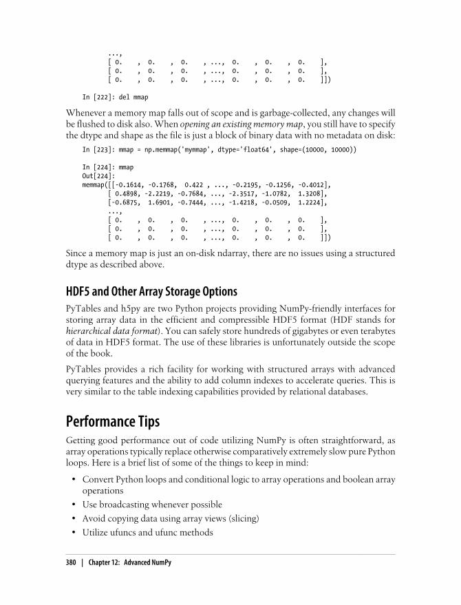
..., [ 0. , 0. , 0. , ..., 0. , 0. , 0. ], [ 0. , 0. , 0. , ..., 0. , 0. , 0. ], [ 0. , 0. , 0. , ..., 0. , 0. , 0. ]])
In [222]: del mmap
Whenever a memory map falls out of scope and is garbage-collected, any changes willbe flushed to disk also. When opening an existing memory map, you still have to specifythe dtype and shape as the file is just a block of binary data with no metadata on disk:
In [223]: mmap = np.memmap('mymmap', dtype='float64', shape=(10000, 10000))
In [224]: mmapOut[224]: memmap([[-0.1614, -0.1768, 0.422 , ..., -0.2195, -0.1256, -0.4012], [ 0.4898, -2.2219, -0.7684, ..., -2.3517, -1.0782, 1.3208], [-0.6875, 1.6901, -0.7444, ..., -1.4218, -0.0509, 1.2224], ..., [ 0. , 0. , 0. , ..., 0. , 0. , 0. ], [ 0. , 0. , 0. , ..., 0. , 0. , 0. ], [ 0. , 0. , 0. , ..., 0. , 0. , 0. ]])
Since a memory map is just an on-disk ndarray, there are no issues using a structureddtype as described above.
HDF5 and Other Array Storage OptionsPyTables and h5py are two Python projects providing NumPy-friendly interfaces forstoring array data in the efficient and compressible HDF5 format (HDF stands forhierarchical data format). You can safely store hundreds of gigabytes or even terabytesof data in HDF5 format. The use of these libraries is unfortunately outside the scopeof the book.
PyTables provides a rich facility for working with structured arrays with advancedquerying features and the ability to add column indexes to accelerate queries. This isvery similar to the table indexing capabilities provided by relational databases.
Performance TipsGetting good performance out of code utilizing NumPy is often straightforward, asarray operations typically replace otherwise comparatively extremely slow pure Pythonloops. Here is a brief list of some of the things to keep in mind:
• Convert Python loops and conditional logic to array operations and boolean arrayoperations
• Use broadcasting whenever possible
• Avoid copying data using array views (slicing)
• Utilize ufuncs and ufunc methods
380 | Chapter 12: Advanced NumPy

If you can’t get the performance you require after exhausting the capabilities providedby NumPy alone, writing code in C, Fortran, or especially Cython (see a bit more onthis below) may be in order. I personally use Cython (http://cython.org) heavily in myown work as an easy way to get C-like performance with minimal development.
The Importance of Contiguous MemoryWhile the full extent of this topic is a bit outside the scope of this book, in some ap-plications the memory layout of an array can significantly affect the speed of compu-tations. This is based partly on performance differences having to do with the cachehierarchy of the CPU; operations accessing contiguous blocks of memory (for example,summing the rows of a C order array) will generally be the fastest because the memorysubsystem will buffer the appropriate blocks of memory into the ultrafast L1 or L2 CPUcache. Also, certain code paths inside NumPy’s C codebase have been optimized forthe contiguous case in which generic strided memory access can be avoided.
To say that an array’s memory layout is contiguous means that the elements are storedin memory in the order that they appear in the array with respect to Fortran (columnmajor) or C (row major) ordering. By default, NumPy arrays are created as C-contigu-ous or just simply contiguous. A column major array, such as the transpose of a C-contiguous array, is thus said to be Fortran-contiguous. These properties can be ex-plicitly checked via the flags attribute on the ndarray:
In [227]: arr_c = np.ones((1000, 1000), order='C')
In [228]: arr_f = np.ones((1000, 1000), order='F')
In [229]: arr_c.flags In [230]: arr_f.flags Out[229]: Out[230]: C_CONTIGUOUS : True C_CONTIGUOUS : False F_CONTIGUOUS : False F_CONTIGUOUS : True OWNDATA : True OWNDATA : True WRITEABLE : True WRITEABLE : True ALIGNED : True ALIGNED : True UPDATEIFCOPY : False UPDATEIFCOPY : False In [231]: arr_f.flags.f_contiguousOut[231]: True
In this example, summing the rows of these arrays should, in theory, be faster forarr_c than arr_f since the rows are contiguous in memory. Here I check for sure using%timeit in IPython:
In [232]: %timeit arr_c.sum(1)1000 loops, best of 3: 1.33 ms per loop
In [233]: %timeit arr_f.sum(1)100 loops, best of 3: 8.75 ms per loop
Performance Tips | 381

When looking to squeeze more performance out of NumPy, this is often a place toinvest some effort. If you have an array that does not have the desired memory order,you can use copy and pass either 'C' or 'F':
In [234]: arr_f.copy('C').flagsOut[234]: C_CONTIGUOUS : True F_CONTIGUOUS : False OWNDATA : True WRITEABLE : True ALIGNED : True UPDATEIFCOPY : False
When constructing a view on an array, keep in mind that the result is not guaranteedto be contiguous:
In [235]: arr_c[:50].flags.contiguous In [236]: arr_c[:, :50].flagsOut[235]: True Out[236]: C_CONTIGUOUS : False F_CONTIGUOUS : False OWNDATA : False WRITEABLE : True ALIGNED : True UPDATEIFCOPY : False
Other Speed Options: Cython, f2py, CIn recent years, the Cython project ((http://cython.org) has become the tool of choicefor many scientific Python programmers for implementing fast code that may need tointeract with C or C++ libraries, but without having to write pure C code. You canthink of Cython as Python with static types and the ability to interleave functions im-plemented in C into Python-like code. For example, a simple Cython function to sumthe elements of a one-dimensional array might look like:
from numpy cimport ndarray, float64_t
def sum_elements(ndarray[float64_t] arr): cdef Py_ssize_t i, n = len(arr) cdef float64_t result = 0
for i in range(n): result += arr[i]
return result
Cython takes this code, translates it to C, then compiles the generated C code to createa Python extension. Cython is an attractive option for performance computing becausethe code is only slightly more time-consuming to write than pure Python code and itintegrates closely with NumPy. A common workflow is to get an algorithm working inPython, then translate it to Cython by adding type declarations and a handful of othertweaks. For more, see the project documentation.
382 | Chapter 12: Advanced NumPy

Some other options for writing high performance code with NumPy include f2py, awrapper generator for Fortran 77 and 90 code, and writing pure C extensions.
Performance Tips | 383


APPENDIX
Python Language Essentials
Knowledge is a treasure, but practice is the key to it.
—Thomas Fuller
People often ask me about good resources for learning Python for data-centric appli-cations. While there are many excellent Python language books, I am usually hesitantto recommend some of them as they are intended for a general audience rather thantailored for someone who wants to load in some data sets, do some computations, andplot some of the results. There are actually a couple of books on “scientific program-ming in Python”, but they are geared toward numerical computing and engineeringapplications: solving differential equations, computing integrals, doing Monte Carlosimulations, and various topics that are more mathematically-oriented rather than be-ing about data analysis and statistics. As this is a book about becoming proficient atworking with data in Python, I think it is valuable to spend some time highlighting themost important features of Python’s built-in data structures and libraries from the per-spective of processing and manipulating structured and unstructured data. As such, Iwill only present roughly enough information to enable you to follow along with therest of the book.
This chapter is not intended to be an exhaustive introduction to the Python languagebut rather a biased, no-frills overview of features which are used repeatedly throughoutthis book. For new Python programmers, I recommend that you supplement this chap-ter with the official Python tutorial (http://docs.python.org) and potentially one of themany excellent (and much longer) books on general purpose Python programming. Inmy opinion, it is not necessary to become proficient at building good software in Pythonto be able to productively do data analysis. I encourage you to use IPython to experi-ment with the code examples and to explore the documentation for the various types,functions, and methods. Note that some of the code used in the examples may notnecessarily be fully-introduced at this point.
Much of this book focuses on high performance array-based computing tools for work-ing with large data sets. In order to use those tools you must often first do some mungingto corral messy data into a more nicely structured form. Fortunately, Python is one of
385
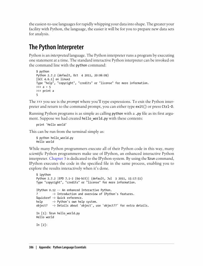
the easiest-to-use languages for rapidly whipping your data into shape. The greater yourfacility with Python, the language, the easier it will be for you to prepare new data setsfor analysis.
The Python InterpreterPython is an interpreted language. The Python interpreter runs a program by executingone statement at a time. The standard interactive Python interpreter can be invoked onthe command line with the python command:
$ pythonPython 2.7.2 (default, Oct 4 2011, 20:06:09)[GCC 4.6.1] on linux2Type "help", "copyright", "credits" or "license" for more information.>>> a = 5>>> print a5
The >>> you see is the prompt where you’ll type expressions. To exit the Python inter-preter and return to the command prompt, you can either type exit() or press Ctrl-D.
Running Python programs is as simple as calling python with a .py file as its first argu-ment. Suppose we had created hello_world.py with these contents:
print 'Hello world'
This can be run from the terminal simply as:
$ python hello_world.pyHello world
While many Python programmers execute all of their Python code in this way, manyscientific Python programmers make use of IPython, an enhanced interactive Pythoninterpreter. Chapter 3 is dedicated to the IPython system. By using the %run command,IPython executes the code in the specified file in the same process, enabling you toexplore the results interactively when it’s done.
$ ipythonPython 2.7.2 |EPD 7.1-2 (64-bit)| (default, Jul 3 2011, 15:17:51)Type "copyright", "credits" or "license" for more information.
IPython 0.12 -- An enhanced Interactive Python.? -> Introduction and overview of IPython's features.%quickref -> Quick reference.help -> Python's own help system.object? -> Details about 'object', use 'object??' for extra details.
In [1]: %run hello_world.pyHello world
In [2]:
386 | Appendix: Python Language Essentials

The default IPython prompt adopts the numbered In [2]: style compared with thestandard >>> prompt.
The Basics
Language SemanticsThe Python language design is distinguished by its emphasis on readability, simplicity,and explicitness. Some people go so far as to liken it to “executable pseudocode”.
Indentation, not braces
Python uses whitespace (tabs or spaces) to structure code instead of using braces as inmany other languages like R, C++, Java, and Perl. Take the for loop in the abovequicksort algorithm:
for x in array: if x < pivot: less.append(x) else: greater.append(x)
A colon denotes the start of an indented code block after which all of the code must beindented by the same amount until the end of the block. In another language, you mightinstead have something like:
for x in array { if x < pivot { less.append(x) } else { greater.append(x) } }
One major reason that whitespace matters is that it results in most Python code lookingcosmetically similar, which means less cognitive dissonance when you read a piece ofcode that you didn’t write yourself (or wrote in a hurry a year ago!). In a languagewithout significant whitespace, you might stumble on some differently formatted codelike:
for x in array { if x < pivot { less.append(x) } else { greater.append(x)
The Basics | 387
} }
Love it or hate it, significant whitespace is a fact of life for Python programmers, andin my experience it helps make Python code a lot more readable than other languagesI’ve used. While it may seem foreign at first, I suspect that it will grow on you after awhile.
I strongly recommend that you use 4 spaces to as your default indenta-tion and that your editor replace tabs with 4 spaces. Many text editorshave a setting that will replace tab stops with spaces automatically (dothis!). Some people use tabs or a different number of spaces, with 2spaces not being terribly uncommon. 4 spaces is by and large the stan-dard adopted by the vast majority of Python programmers, so I recom-mend doing that in the absence of a compelling reason otherwise.
As you can see by now, Python statements also do not need to be terminated by sem-icolons. Semicolons can be used, however, to separate multiple statements on a singleline:
a = 5; b = 6; c = 7
Putting multiple statements on one line is generally discouraged in Python as it oftenmakes code less readable.
Everything is an object
An important characteristic of the Python language is the consistency of its objectmodel. Every number, string, data structure, function, class, module, and so on existsin the Python interpreter in its own “box” which is referred to as a Python object. Eachobject has an associated type (for example, string or function) and internal data. Inpractice this makes the language very flexible, as even functions can be treated just likeany other object.
Comments
Any text preceded by the hash mark (pound sign) # is ignored by the Python interpreter.This is often used to add comments to code. At times you may also want to excludecertain blocks of code without deleting them. An easy solution is to comment out thecode:
results = []for line in file_handle: # keep the empty lines for now # if len(line) == 0: # continue results.append(line.replace('foo', 'bar'))
388 | Appendix: Python Language Essentials
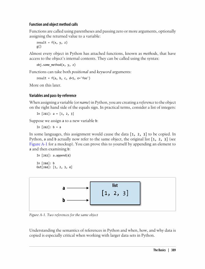
Function and object method calls
Functions are called using parentheses and passing zero or more arguments, optionallyassigning the returned value to a variable:
result = f(x, y, z)g()
Almost every object in Python has attached functions, known as methods, that haveaccess to the object’s internal contents. They can be called using the syntax:
obj.some_method(x, y, z)
Functions can take both positional and keyword arguments:
result = f(a, b, c, d=5, e='foo')
Variables and pass-by-reference
When assigning a variable (or name) in Python, you are creating a reference to the objecton the right hand side of the equals sign. In practical terms, consider a list of integers:
In [241]: a = [1, 2, 3]
Suppose we assign a to a new variable b:
In [242]: b = a
In some languages, this assignment would cause the data [1, 2, 3] to be copied. InPython, a and b actually now refer to the same object, the original list [1, 2, 3] (seeFigure A-1 for a mockup). You can prove this to yourself by appending an element toa and then examining b:
In [243]: a.append(4)
In [244]: bOut[244]: [1, 2, 3, 4]
Figure A-1. Two references for the same object
Understanding the semantics of references in Python and when, how, and why data iscopied is especially critical when working with larger data sets in Python.
The Basics | 389

Assignment is also referred to as binding, as we are binding a name toan object. Variables names that have been assigned may occasionally bereferred to as bound variables.
When you pass objects as arguments to a function, you are only passing references; nocopying occurs. Thus, Python is said to pass by reference, whereas some other languagessupport both pass by value (creating copies) and pass by reference. This means that afunction can mutate the internals of its arguments. Suppose we had the following func-tion:
def append_element(some_list, element): some_list.append(element)
Then given what’s been said, this should not come as a surprise:
In [2]: data = [1, 2, 3]
In [3]: append_element(data, 4)
In [4]: dataOut[4]: [1, 2, 3, 4]
Dynamic references, strong types
In contrast with many compiled languages, such as Java and C++, object references inPython have no type associated with them. There is no problem with the following:
In [245]: a = 5 In [246]: type(a) Out[246]: int In [247]: a = 'foo' In [248]: type(a) Out[248]: str
Variables are names for objects within a particular namespace; the type information isstored in the object itself. Some observers might hastily conclude that Python is not a“typed language”. This is not true; consider this example:
In [249]: '5' + 5---------------------------------------------------------------------------TypeError Traceback (most recent call last)<ipython-input-249-f9dbf5f0b234> in <module>()----> 1 '5' + 5TypeError: cannot concatenate 'str' and 'int' objects
In some languages, such as Visual Basic, the string '5' might get implicitly converted(or casted) to an integer, thus yielding 10. Yet in other languages, such as JavaScript,the integer 5 might be casted to a string, yielding the concatenated string '55'. In thisregard Python is considered a strongly-typed language, which means that every objecthas a specific type (or class), and implicit conversions will occur only in certain obviouscircumstances, such as the following:
390 | Appendix: Python Language Essentials

In [250]: a = 4.5
In [251]: b = 2
# String formatting, to be visited laterIn [252]: print 'a is %s, b is %s' % (type(a), type(b))a is <type 'float'>, b is <type 'int'>
In [253]: a / bOut[253]: 2.25
Knowing the type of an object is important, and it’s useful to be able to write functionsthat can handle many different kinds of input. You can check that an object is aninstance of a particular type using the isinstance function:
In [254]: a = 5 In [255]: isinstance(a, int) Out[255]: True
isinstance can accept a tuple of types if you want to check that an object’s type isamong those present in the tuple:
In [256]: a = 5; b = 4.5
In [257]: isinstance(a, (int, float)) In [258]: isinstance(b, (int, float))Out[257]: True Out[258]: True
Attributes and methods
Objects in Python typically have both attributes, other Python objects stored “inside”the object, and methods, functions associated with an object which can have access tothe object’s internal data. Both of them are accessed via the syntax obj.attribute_name:
In [1]: a = 'foo'
In [2]: a.<Tab>a.capitalize a.format a.isupper a.rindex a.stripa.center a.index a.join a.rjust a.swapcasea.count a.isalnum a.ljust a.rpartition a.titlea.decode a.isalpha a.lower a.rsplit a.translatea.encode a.isdigit a.lstrip a.rstrip a.uppera.endswith a.islower a.partition a.split a.zfilla.expandtabs a.isspace a.replace a.splitlinesa.find a.istitle a.rfind a.startswith
Attributes and methods can also be accessed by name using the getattr function:
>>> getattr(a, 'split')<function split>
While we will not extensively use the functions getattr and related functions hasattrand setattr in this book, they can be used very effectively to write generic, reusablecode.
The Basics | 391

“Duck” typing
Often you may not care about the type of an object but rather only whether it has certainmethods or behavior. For example, you can verify that an object is iterable if it imple-mented the iterator protocol. For many objects, this means it has a __iter__ “magicmethod”, though an alternative and better way to check is to try using the iter function:
def isiterable(obj): try: iter(obj) return True except TypeError: # not iterable return False
This function would return True for strings as well as most Python collection types:
In [260]: isiterable('a string') In [261]: isiterable([1, 2, 3])Out[260]: True Out[261]: True In [262]: isiterable(5)Out[262]: False
A place where I use this functionality all the time is to write functions that can acceptmultiple kinds of input. A common case is writing a function that can accept any kindof sequence (list, tuple, ndarray) or even an iterator. You can first check if the object isa list (or a NumPy array) and, if it is not, convert it to be one:
if not isinstance(x, list) and isiterable(x): x = list(x)
Imports
In Python a module is simply a .py file containing function and variable definitionsalong with such things imported from other .py files. Suppose that we had the followingmodule:
# some_module.pyPI = 3.14159
def f(x): return x + 2
def g(a, b): return a + b
If we wanted to access the variables and functions defined in some_module.py, fromanother file in the same directory we could do:
import some_moduleresult = some_module.f(5)pi = some_module.PI
Or equivalently:
from some_module import f, g, PIresult = g(5, PI)
392 | Appendix: Python Language Essentials
By using the as keyword you can give imports different variable names:
import some_module as smfrom some_module import PI as pi, g as gf
r1 = sm.f(pi)r2 = gf(6, pi)
Binary operators and comparisons
Most of the binary math operations and comparisons are as you might expect:
In [263]: 5 - 7 In [264]: 12 + 21.5Out[263]: -2 Out[264]: 33.5 In [265]: 5 <= 2Out[265]: False
See Table A-1 for all of the available binary operators.
To check if two references refer to the same object, use the is keyword. is not is alsoperfectly valid if you want to check that two objects are not the same:
In [266]: a = [1, 2, 3]
In [267]: b = a
# Note, the list function always creates a new listIn [268]: c = list(a)
In [269]: a is b In [270]: a is not cOut[269]: True Out[270]: True
Note this is not the same thing is comparing with ==, because in this case we have:
In [271]: a == cOut[271]: True
A very common use of is and is not is to check if a variable is None, since there is onlyone instance of None:
In [272]: a = None
In [273]: a is NoneOut[273]: True
Table A-1. Binary operators
Operation Description
a + b Add a and b
a - b Subtract b from a
a * b Multiply a by b
a / b Divide a by b
a // b Floor-divide a by b, dropping any fractional remainder
The Basics | 393

Operation Description
a ** b Raise a to the b power
a & b True if both a and b are True. For integers, take the bitwise AND.
a | b True if either a or b is True. For integers, take the bitwise OR.
a ^ b For booleans, True if a or b is True, but not both. For integers, take the bitwise EXCLUSIVE-OR.
a == b True if a equals b
a != b True if a is not equal to b
a <= b, a < b True if a is less than (less than or equal) to b
a > b, a >= b True if a is greater than (greater than or equal) to b
a is b True if a and b reference same Python object
a is not b True if a and b reference different Python objects
Strictness versus laziness
When using any programming language, it’s important to understand when expressionsare evaluated. Consider the simple expression:
a = b = c = 5d = a + b * c
In Python, once these statements are evaluated, the calculation is immediately (orstrictly) carried out, setting the value of d to 30. In another programming paradigm,such as in a pure functional programming language like Haskell, the value of d mightnot be evaluated until it is actually used elsewhere. The idea of deferring computationsin this way is commonly known as lazy evaluation. Python, on the other hand, is a very strict (or eager) language. Nearly all of the time, computations and expressions areevaluated immediately. Even in the above simple expression, the result of b * c iscomputed as a separate step before adding it to a.
There are Python techniques, especially using iterators and generators, which can beused to achieve laziness. When performing very expensive computations which are onlynecessary some of the time, this can be an important technique in data-intensive ap-plications.
Mutable and immutable objects
Most objects in Python are mutable, such as lists, dicts, NumPy arrays, or most user-defined types (classes). This means that the object or values that they contain can bemodified.
In [274]: a_list = ['foo', 2, [4, 5]]
In [275]: a_list[2] = (3, 4)
In [276]: a_listOut[276]: ['foo', 2, (3, 4)]
394 | Appendix: Python Language Essentials

Others, like strings and tuples, are immutable:
In [277]: a_tuple = (3, 5, (4, 5))
In [278]: a_tuple[1] = 'four'---------------------------------------------------------------------------TypeError Traceback (most recent call last)<ipython-input-278-b7966a9ae0f1> in <module>()----> 1 a_tuple[1] = 'four'TypeError: 'tuple' object does not support item assignment
Remember that just because you can mutate an object does not mean that you alwaysshould. Such actions are known in programming as side effects. For example, whenwriting a function, any side effects should be explicitly communicated to the user inthe function’s documentation or comments. If possible, I recommend trying to avoidside effects and favor immutability, even though there may be mutable objects involved.
Scalar TypesPython has a small set of built-in types for handling numerical data, strings, boolean(True or False) values, and dates and time. See Table A-2 for a list of the main scalartypes. Date and time handling will be discussed separately as these are provided by the datetime module in the standard library.
Table A-2. Standard Python Scalar Types
Type Description
None The Python “null” value (only one instance of the None object exists)
str String type. ASCII-valued only in Python 2.x and Unicode in Python 3
unicode Unicode string type
float Double-precision (64-bit) floating point number. Note there is no separate double type.
bool A True or False value
int Signed integer with maximum value determined by the platform.
long Arbitrary precision signed integer. Large int values are automatically converted to long.
Numeric types
The primary Python types for numbers are int and float. The size of the integer whichcan be stored as an int is dependent on your platform (whether 32 or 64-bit), but Pythonwill transparently convert a very large integer to long, which can store arbitrarily largeintegers.
In [279]: ival = 17239871
In [280]: ival ** 6Out[280]: 26254519291092456596965462913230729701102721L
The Basics | 395
Floating point numbers are represented with the Python float type. Under the hoodeach one is a double-precision (64 bits) value. They can also be expressed using scien-tific notation:
In [281]: fval = 7.243
In [282]: fval2 = 6.78e-5
In Python 3, integer division not resulting in a whole number will always yield a floatingpoint number:
In [284]: 3 / 2Out[284]: 1.5
In Python 2.7 and below (which some readers will likely be using), you can enable thisbehavior by default by putting the following cryptic-looking statement at the top ofyour module:
from __future__ import division
Without this in place, you can always explicitly convert the denominator into a floatingpoint number:
In [285]: 3 / float(2)Out[285]: 1.5
To get C-style integer division (which drops the fractional part if the result is not awhole number), use the floor division operator //:
In [286]: 3 // 2Out[286]: 1
Complex numbers are written using j for the imaginary part:
In [287]: cval = 1 + 2j
In [288]: cval * (1 - 2j)Out[288]: (5+0j)
Strings
Many people use Python for its powerful and flexible built-in string processing capa-bilities. You can write string literal using either single quotes ' or double quotes ":
a = 'one way of writing a string'b = "another way"
For multiline strings with line breaks, you can use triple quotes, either ''' or """:
c = """This is a longer string thatspans multiple lines"""
Python strings are immutable; you cannot modify a string without creating a new string:
396 | Appendix: Python Language Essentials

In [289]: a = 'this is a string'
In [290]: a[10] = 'f'---------------------------------------------------------------------------TypeError Traceback (most recent call last)<ipython-input-290-5ca625d1e504> in <module>()----> 1 a[10] = 'f'TypeError: 'str' object does not support item assignment
In [291]: b = a.replace('string', 'longer string')
In [292]: bOut[292]: 'this is a longer string'
Many Python objects can be converted to a string using the str function:
In [293]: a = 5.6 In [294]: s = str(a) In [295]: sOut[295]: '5.6'
Strings are a sequence of characters and therefore can be treated like other sequences,such as lists and tuples:
In [296]: s = 'python' In [297]: list(s) Out[297]: ['p', 'y', 't', 'h', 'o', 'n'] In [298]: s[:3]Out[298]: 'pyt'
The backslash character \ is an escape character, meaning that it is used to specifyspecial characters like newline \n or unicode characters. To write a string literal withbackslashes, you need to escape them:
In [299]: s = '12\\34'
In [300]: print s12\34
If you have a string with a lot of backslashes and no special characters, you might findthis a bit annoying. Fortunately you can preface the leading quote of the string with rwhich means that the characters should be interpreted as is:
In [301]: s = r'this\has\no\special\characters'
In [302]: sOut[302]: 'this\\has\\no\\special\\characters'
Adding two strings together concatenates them and produces a new string:
In [303]: a = 'this is the first half '
In [304]: b = 'and this is the second half'
In [305]: a + bOut[305]: 'this is the first half and this is the second half'
The Basics | 397

String templating or formatting is another important topic. The number of ways to doso has expanded with the advent of Python 3, here I will briefly describe the mechanicsof one of the main interfaces. Strings with a % followed by one or more format charactersis a target for inserting a value into that string (this is quite similar to the printf functionin C). As an example, consider this string:
In [306]: template = '%.2f %s are worth $%d'
In this string, %s means to format an argument as a string, %.2f a number with 2 decimalplaces, and %d an integer. To substitute arguments for these format parameters, use thebinary operator % with a tuple of values:
In [307]: template % (4.5560, 'Argentine Pesos', 1)Out[307]: '4.56 Argentine Pesos are worth $1'
String formatting is a broad topic; there are multiple methods and numerous optionsand tweaks available to control how values are formatted in the resulting string. Tolearn more, I recommend you seek out more information on the web.
I discuss general string processing as it relates to data analysis in more detail in Chap-ter 7.
Booleans
The two boolean values in Python are written as True and False. Comparisons andother conditional expressions evaluate to either True or False. Boolean values are com-bined with the and and or keywords:
In [308]: True and TrueOut[308]: True
In [309]: False or TrueOut[309]: True
Almost all built-in Python tops and any class defining the __nonzero__ magic methodhave a True or False interpretation in an if statement:
In [310]: a = [1, 2, 3] .....: if a: .....: print 'I found something!' .....:I found something!
In [311]: b = [] .....: if not b: .....: print 'Empty!' .....:Empty!
Most objects in Python have a notion of true- or falseness. For example, empty se-quences (lists, dicts, tuples, etc.) are treated as False if used in control flow (as abovewith the empty list b). You can see exactly what boolean value an object coerces to byinvoking bool on it:
398 | Appendix: Python Language Essentials
In [312]: bool([]), bool([1, 2, 3])Out[312]: (False, True)
In [313]: bool('Hello world!'), bool('')Out[313]: (True, False)
In [314]: bool(0), bool(1)Out[314]: (False, True)
Type casting
The str, bool, int and float types are also functions which can be used to cast valuesto those types:
In [315]: s = '3.14159'
In [316]: fval = float(s) In [317]: type(fval) Out[317]: float In [318]: int(fval) In [319]: bool(fval) In [320]: bool(0)Out[318]: 3 Out[319]: True Out[320]: False
None
None is the Python null value type. If a function does not explicitly return a value, itimplicitly returns None.
In [321]: a = None In [322]: a is None Out[322]: True In [323]: b = 5 In [324]: b is not None Out[324]: True
None is also a common default value for optional function arguments:
def add_and_maybe_multiply(a, b, c=None): result = a + b
if c is not None: result = result * c
return result
While a technical point, it’s worth bearing in mind that None is not a reserved keywordbut rather a unique instance of NoneType.
Dates and times
The built-in Python datetime module provides datetime, date, and time types. Thedatetime type as you may imagine combines the information stored in date and timeand is the most commonly used:
In [325]: from datetime import datetime, date, time
In [326]: dt = datetime(2011, 10, 29, 20, 30, 21)
The Basics | 399

In [327]: dt.day In [328]: dt.minuteOut[327]: 29 Out[328]: 30
Given a datetime instance, you can extract the equivalent date and time objects bycalling methods on the datetime of the same name:
In [329]: dt.date() In [330]: dt.time() Out[329]: datetime.date(2011, 10, 29) Out[330]: datetime.time(20, 30, 21)
The strftime method formats a datetime as a string:
In [331]: dt.strftime('%m/%d/%Y %H:%M')Out[331]: '10/29/2011 20:30'
Strings can be converted (parsed) into datetime objects using the strptime function:
In [332]: datetime.strptime('20091031', '%Y%m%d')Out[332]: datetime.datetime(2009, 10, 31, 0, 0)
See Table 10-2 for a full list of format specifications.
When aggregating of otherwise grouping time series data, it will occasionally be usefulto replace fields of a series of datetimes, for example replacing the minute and secondfields with zero, producing a new object:
In [333]: dt.replace(minute=0, second=0)Out[333]: datetime.datetime(2011, 10, 29, 20, 0)
The difference of two datetime objects produces a datetime.timedelta type:
In [334]: dt2 = datetime(2011, 11, 15, 22, 30)
In [335]: delta = dt2 - dt
In [336]: delta In [337]: type(delta) Out[336]: datetime.timedelta(17, 7179) Out[337]: datetime.timedelta
Adding a timedelta to a datetime produces a new shifted datetime:
In [338]: dtOut[338]: datetime.datetime(2011, 10, 29, 20, 30, 21)
In [339]: dt + deltaOut[339]: datetime.datetime(2011, 11, 15, 22, 30)
Control Flow
if, elif, and else
The if statement is one of the most well-known control flow statement types. It checksa condition which, if True, evaluates the code in the block that follows:
if x < 0: print 'It's negative'
400 | Appendix: Python Language Essentials

An if statement can be optionally followed by one or more elif blocks and a catch-allelse block if all of the conditions are False:
if x < 0: print 'It's negative'elif x == 0: print 'Equal to zero'elif 0 < x < 5: print 'Positive but smaller than 5'else: print 'Positive and larger than or equal to 5'
If any of the conditions is True, no further elif or else blocks will be reached. With acompound condition using and or or, conditions are evaluated left-to-right and willshort circuit:
In [340]: a = 5; b = 7
In [341]: c = 8; d = 4
In [342]: if a < b or c > d: .....: print 'Made it'Made it
In this example, the comparison c > d never gets evaluated because the first comparisonwas True.
for loops
for loops are for iterating over a collection (like a list or tuple) or an iterater. Thestandard syntax for a for loop is:
for value in collection: # do something with value
A for loop can be advanced to the next iteration, skipping the remainder of the block,using the continue keyword. Consider this code which sums up integers in a list andskips None values:
sequence = [1, 2, None, 4, None, 5]total = 0for value in sequence: if value is None: continue total += value
A for loop can be exited altogether using the break keyword. This code sums elementsof the list until a 5 is reached:
sequence = [1, 2, 0, 4, 6, 5, 2, 1]total_until_5 = 0for value in sequence: if value == 5: break total_until_5 += value
The Basics | 401

As we will see in more detail, if the elements in the collection or iterator are sequences(tuples or lists, say), they can be conveniently unpacked into variables in the for loopstatement:
for a, b, c in iterator: # do something
while loops
A while loop specifies a condition and a block of code that is to be executed until thecondition evaluates to False or the loop is explicitly ended with break:
x = 256total = 0while x > 0: if total > 500: break total += x x = x // 2
pass
pass is the “no-op” statement in Python. It can be used in blocks where no action is tobe taken; it is only required because Python uses whitespace to delimit blocks:
if x < 0: print 'negative!'elif x == 0: # TODO: put something smart here passelse: print 'positive!'
It’s common to use pass as a place-holder in code while working on a new piece offunctionality:
def f(x, y, z): # TODO: implement this function! pass
Exception handling
Handling Python errors or exceptions gracefully is an important part of building robustprograms. In data analysis applications, many functions only work on certain kinds ofinput. As an example, Python’s float function is capable of casting a string to a floatingpoint number, but fails with ValueError on improper inputs:
In [343]: float('1.2345')Out[343]: 1.2345
In [344]: float('something')---------------------------------------------------------------------------ValueError Traceback (most recent call last)<ipython-input-344-439904410854> in <module>()
402 | Appendix: Python Language Essentials

----> 1 float('something')ValueError: could not convert string to float: something
Suppose we wanted a version of float that fails gracefully, returning the input argu-ment. We can do this by writing a function that encloses the call to float in a try/except block:
def attempt_float(x): try: return float(x) except: return x
The code in the except part of the block will only be executed if float(x) raises anexception:
In [346]: attempt_float('1.2345')Out[346]: 1.2345
In [347]: attempt_float('something')Out[347]: 'something'
You might notice that float can raise exceptions other than ValueError:
In [348]: float((1, 2))---------------------------------------------------------------------------TypeError Traceback (most recent call last)<ipython-input-348-842079ebb635> in <module>()----> 1 float((1, 2))TypeError: float() argument must be a string or a number
You might want to only suppress ValueError, since a TypeError (the input was not astring or numeric value) might indicate a legitimate bug in your program. To do that,write the exception type after except:
def attempt_float(x): try: return float(x) except ValueError: return x
We have then:
In [350]: attempt_float((1, 2))---------------------------------------------------------------------------TypeError Traceback (most recent call last)<ipython-input-350-9bdfd730cead> in <module>()----> 1 attempt_float((1, 2))<ipython-input-349-3e06b8379b6b> in attempt_float(x) 1 def attempt_float(x): 2 try:----> 3 return float(x) 4 except ValueError: 5 return xTypeError: float() argument must be a string or a number
The Basics | 403
You can catch multiple exception types by writing a tuple of exception types instead(the parentheses are required):
def attempt_float(x): try: return float(x) except (TypeError, ValueError): return x
In some cases, you may not want to suppress an exception, but you want some codeto be executed regardless of whether the code in the try block succeeds or not. To dothis, use finally:
f = open(path, 'w')
try: write_to_file(f)finally: f.close()
Here, the file handle f will always get closed. Similarly, you can have code that executesonly if the try: block succeeds using else:
f = open(path, 'w')
try: write_to_file(f)except: print 'Failed'else: print 'Succeeded'finally: f.close()
range and xrange
The range function produces a list of evenly-spaced integers:
In [352]: range(10)Out[352]: [0, 1, 2, 3, 4, 5, 6, 7, 8, 9]
Both a start, end, and step can be given:
In [353]: range(0, 20, 2)Out[353]: [0, 2, 4, 6, 8, 10, 12, 14, 16, 18]
As you can see, range produces integers up to but not including the endpoint. A com-mon use of range is for iterating through sequences by index:
seq = [1, 2, 3, 4]for i in range(len(seq)): val = seq[i]
For very long ranges, it’s recommended to use xrange, which takes the same argumentsas range but returns an iterator that generates integers one by one rather than generating
404 | Appendix: Python Language Essentials
all of them up-front and storing them in a (potentially very large) list. This snippet sumsall numbers from 0 to 9999 that are multiples of 3 or 5:
sum = 0for i in xrange(10000): # % is the modulo operator if x % 3 == 0 or x % 5 == 0: sum += i
In Python 3, range always returns an iterator, and thus it is not necessaryto use the xrange function
Ternary Expressions
A ternary expression in Python allows you combine an if-else block which producesa value into a single line or expression. The syntax for this in Python is
value = true-expr if condition elsefalse-expr
Here, true-expr and false-expr can be any Python expressions. It has the identicaleffect as the more verbose
if condition: value = true-exprelse: value = false-expr
This is a more concrete example:
In [354]: x = 5
In [355]: 'Non-negative' if x >= 0 else 'Negative'Out[355]: 'Non-negative'
As with if-else blocks, only one of the expressions will be evaluated. While it may betempting to always use ternary expressions to condense your code, realize that you maysacrifice readability if the condition as well and the true and false expressions are verycomplex.
Data Structures and SequencesPython’s data structures are simple, but powerful. Mastering their use is a critical partof becoming a proficient Python programmer.
Data Structures and Sequences | 405

TupleA tuple is a one-dimensional, fixed-length, immutable sequence of Python objects. Theeasiest way to create one is with a comma-separated sequence of values:
In [356]: tup = 4, 5, 6
In [357]: tupOut[357]: (4, 5, 6)
When defining tuples in more complicated expressions, it’s often necessary to enclosethe values in parentheses, as in this example of creating a tuple of tuples:
In [358]: nested_tup = (4, 5, 6), (7, 8)
In [359]: nested_tupOut[359]: ((4, 5, 6), (7, 8))
Any sequence or iterator can be converted to a tuple by invoking tuple:
In [360]: tuple([4, 0, 2])Out[360]: (4, 0, 2)
In [361]: tup = tuple('string')
In [362]: tupOut[362]: ('s', 't', 'r', 'i', 'n', 'g')
Elements can be accessed with square brackets [] as with most other sequence types.Like C, C++, Java, and many other languages, sequences are 0-indexed in Python:
In [363]: tup[0]Out[363]: 's'
While the objects stored in a tuple may be mutable themselves, once created it’s notpossible to modify which object is stored in each slot:
In [364]: tup = tuple(['foo', [1, 2], True])
In [365]: tup[2] = False---------------------------------------------------------------------------TypeError Traceback (most recent call last)<ipython-input-365-c7308343b841> in <module>()----> 1 tup[2] = FalseTypeError: 'tuple' object does not support item assignment
# howeverIn [366]: tup[1].append(3)
In [367]: tupOut[367]: ('foo', [1, 2, 3], True)
Tuples can be concatenated using the + operator to produce longer tuples:
In [368]: (4, None, 'foo') + (6, 0) + ('bar',)Out[368]: (4, None, 'foo', 6, 0, 'bar')
406 | Appendix: Python Language Essentials

Multiplying a tuple by an integer, as with lists, has the effect of concatenating togetherthat many copies of the tuple.
In [369]: ('foo', 'bar') * 4Out[369]: ('foo', 'bar', 'foo', 'bar', 'foo', 'bar', 'foo', 'bar')
Note that the objects themselves are not copied, only the references to them.
Unpacking tuples
If you try to assign to a tuple-like expression of variables, Python will attempt to un-pack the value on the right-hand side of the equals sign:
In [370]: tup = (4, 5, 6)
In [371]: a, b, c = tup
In [372]: bOut[372]: 5
Even sequences with nested tuples can be unpacked:
In [373]: tup = 4, 5, (6, 7)
In [374]: a, b, (c, d) = tup
In [375]: dOut[375]: 7
Using this functionality it’s easy to swap variable names, a task which in many lan-guages might look like:
tmp = aa = bb = tmp
b, a = a, b
One of the most common uses of variable unpacking when iterating over sequences oftuples or lists:
seq = [(1, 2, 3), (4, 5, 6), (7, 8, 9)]for a, b, c in seq: pass
Another common use is for returning multiple values from a function. More on thislater.
Tuple methods
Since the size and contents of a tuple cannot be modified, it is very light on instancemethods. One particularly useful one (also available on lists) is count, which counts thenumber of occurrences of a value:
In [376]: a = (1, 2, 2, 2, 3, 4, 2)
Data Structures and Sequences | 407

In [377]: a.count(2)Out[377]: 4
ListIn contrast with tuples, lists are variable-length and their contents can be modified.They can be defined using square brackets [] or using the list type function:
In [378]: a_list = [2, 3, 7, None]
In [379]: tup = ('foo', 'bar', 'baz')
In [380]: b_list = list(tup) In [381]: b_list Out[381]: ['foo', 'bar', 'baz'] In [382]: b_list[1] = 'peekaboo' In [383]: b_list Out[383]: ['foo', 'peekaboo', 'baz']
Lists and tuples are semantically similar as one-dimensional sequences of objects andthus can be used interchangeably in many functions.
Adding and removing elements
Elements can be appended to the end of the list with the append method:
In [384]: b_list.append('dwarf')
In [385]: b_listOut[385]: ['foo', 'peekaboo', 'baz', 'dwarf']
Using insert you can insert an element at a specific location in the list:
In [386]: b_list.insert(1, 'red')
In [387]: b_listOut[387]: ['foo', 'red', 'peekaboo', 'baz', 'dwarf']
insert is computationally expensive compared with append as referencesto subsequent elements have to be shifted internally to make room forthe new element.
The inverse operation to insert is pop, which removes and returns an element at aparticular index:
In [388]: b_list.pop(2)Out[388]: 'peekaboo'
In [389]: b_listOut[389]: ['foo', 'red', 'baz', 'dwarf']
Elements can be removed by value using remove, which locates the first such value andremoves it from the last:
408 | Appendix: Python Language Essentials
In [390]: b_list.append('foo')
In [391]: b_list.remove('foo')
In [392]: b_listOut[392]: ['red', 'baz', 'dwarf', 'foo']
If performance is not a concern, by using append and remove, a Python list can be usedas a perfectly suitable “multi-set” data structure.
You can check if a list contains a value using the in keyword:
In [393]: 'dwarf' in b_listOut[393]: True
Note that checking whether a list contains a value is a lot slower than dicts and sets asPython makes a linear scan across the values of the list, whereas the others (based onhash tables) can make the check in constant time.
Concatenating and combining lists
Similar to tuples, adding two lists together with + concatenates them:
In [394]: [4, None, 'foo'] + [7, 8, (2, 3)]Out[394]: [4, None, 'foo', 7, 8, (2, 3)]
If you have a list already defined, you can append multiple elements to it using the extend method:
In [395]: x = [4, None, 'foo']
In [396]: x.extend([7, 8, (2, 3)])
In [397]: xOut[397]: [4, None, 'foo', 7, 8, (2, 3)]
Note that list concatenation is a compartively expensive operation since a new list mustbe created and the objects copied over. Using extend to append elements to an existinglist, especially if you are building up a large list, is usually preferable. Thus,
everything = []for chunk in list_of_lists: everything.extend(chunk)
is faster than than the concatenative alternative
everything = []for chunk in list_of_lists: everything = everything + chunk
Sorting
A list can be sorted in-place (without creating a new object) by calling its sort function:
In [398]: a = [7, 2, 5, 1, 3]
Data Structures and Sequences | 409

In [399]: a.sort()
In [400]: aOut[400]: [1, 2, 3, 5, 7]
sort has a few options that will occasionally come in handy. One is the ability to passa secondary sort key, i.e. a function that produces a value to use to sort the objects. Forexample, we could sort a collection of strings by their lengths:
In [401]: b = ['saw', 'small', 'He', 'foxes', 'six']
In [402]: b.sort(key=len)
In [403]: bOut[403]: ['He', 'saw', 'six', 'small', 'foxes']
Binary search and maintaining a sorted list
The built-in bisect module implements binary-search and insertion into a sorted list.bisect.bisect finds the location where an element should be inserted to keep it sorted,while bisect.insort actually inserts the element into that location:
In [404]: import bisect
In [405]: c = [1, 2, 2, 2, 3, 4, 7]
In [406]: bisect.bisect(c, 2) In [407]: bisect.bisect(c, 5)Out[406]: 4 Out[407]: 6 In [408]: bisect.insort(c, 6)
In [409]: cOut[409]: [1, 2, 2, 2, 3, 4, 6, 7]
The bisect module functions do not check whether the list is sorted asdoing so would be computationally expensive. Thus, using them withan unsorted list will succeed without error but may lead to incorrectresults.
Slicing
You can select sections of list-like types (arrays, tuples, NumPy arrays) by using slicenotation, which in its basic form consists of start:stop passed to the indexing operator[]:
In [410]: seq = [7, 2, 3, 7, 5, 6, 0, 1]
In [411]: seq[1:5]Out[411]: [2, 3, 7, 5]
Slices can also be assigned to with a sequence:
In [412]: seq[3:4] = [6, 3]
410 | Appendix: Python Language Essentials

In [413]: seqOut[413]: [7, 2, 3, 6, 3, 5, 6, 0, 1]
While element at the start index is included, the stop index is not included, so thatthe number of elements in the result is stop - start.
Either the start or stop can be omitted in which case they default to the start of thesequence and the end of the sequence, respectively:
In [414]: seq[:5] In [415]: seq[3:] Out[414]: [7, 2, 3, 6, 3] Out[415]: [6, 3, 5, 6, 0, 1]
Negative indices slice the sequence relative to the end:
In [416]: seq[-4:] In [417]: seq[-6:-2] Out[416]: [5, 6, 0, 1] Out[417]: [6, 3, 5, 6]
Slicing semantics takes a bit of getting used to, especially if you’re coming from R orMATLAB. See Figure A-2 for a helpful illustrating of slicing with positive and negativeintegers.
A step can also be used after a second colon to, say, take every other element:
In [418]: seq[::2]Out[418]: [7, 3, 3, 6, 1]
A clever use of this is to pass -1 which has the useful effect of reversing a list or tuple:
In [419]: seq[::-1]Out[419]: [1, 0, 6, 5, 3, 6, 3, 2, 7]
Figure A-2. Illustration of Python slicing conventions
Built-in Sequence FunctionsPython has a handful of useful sequence functions that you should familiarize yourselfwith and use at any opportunity.
Data Structures and Sequences | 411
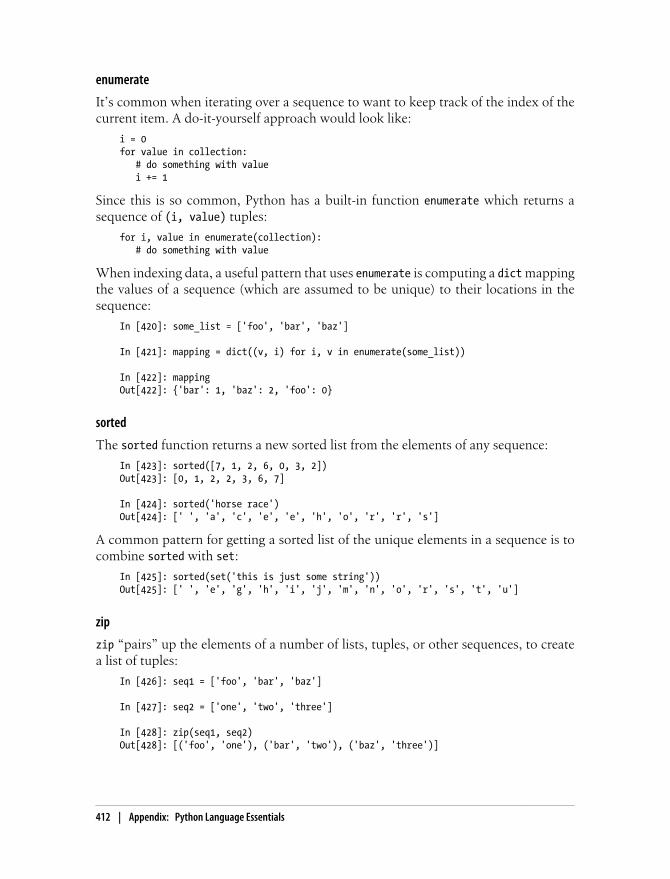
enumerate
It’s common when iterating over a sequence to want to keep track of the index of thecurrent item. A do-it-yourself approach would look like:
i = 0for value in collection: # do something with value i += 1
Since this is so common, Python has a built-in function enumerate which returns asequence of (i, value) tuples:
for i, value in enumerate(collection): # do something with value
When indexing data, a useful pattern that uses enumerate is computing a dict mappingthe values of a sequence (which are assumed to be unique) to their locations in thesequence:
In [420]: some_list = ['foo', 'bar', 'baz']
In [421]: mapping = dict((v, i) for i, v in enumerate(some_list))
In [422]: mappingOut[422]: {'bar': 1, 'baz': 2, 'foo': 0}
sorted
The sorted function returns a new sorted list from the elements of any sequence:
In [423]: sorted([7, 1, 2, 6, 0, 3, 2])Out[423]: [0, 1, 2, 2, 3, 6, 7]
In [424]: sorted('horse race')Out[424]: [' ', 'a', 'c', 'e', 'e', 'h', 'o', 'r', 'r', 's']
A common pattern for getting a sorted list of the unique elements in a sequence is tocombine sorted with set:
In [425]: sorted(set('this is just some string'))Out[425]: [' ', 'e', 'g', 'h', 'i', 'j', 'm', 'n', 'o', 'r', 's', 't', 'u']
zip
zip “pairs” up the elements of a number of lists, tuples, or other sequences, to createa list of tuples:
In [426]: seq1 = ['foo', 'bar', 'baz']
In [427]: seq2 = ['one', 'two', 'three']
In [428]: zip(seq1, seq2)Out[428]: [('foo', 'one'), ('bar', 'two'), ('baz', 'three')]
412 | Appendix: Python Language Essentials
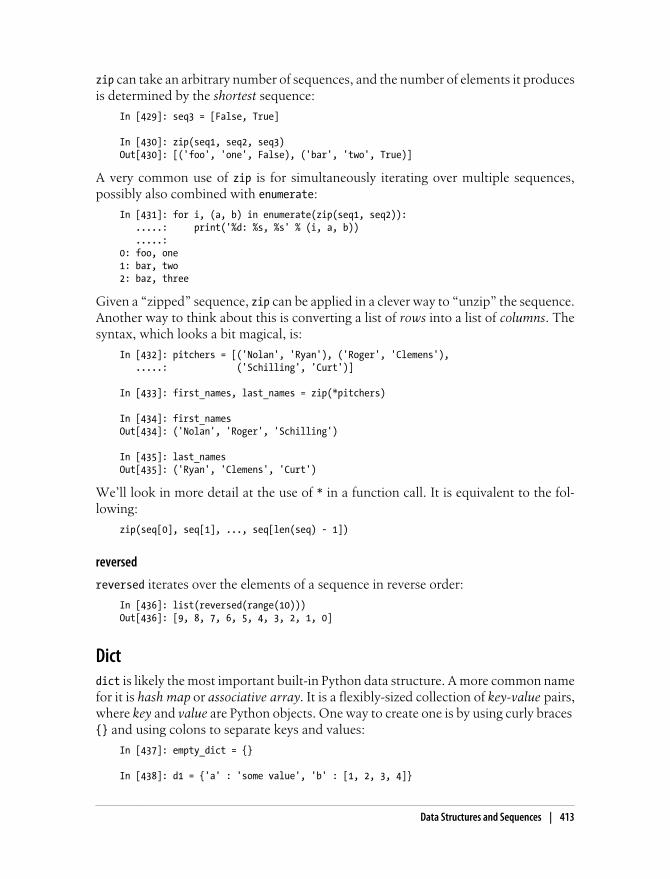
zip can take an arbitrary number of sequences, and the number of elements it producesis determined by the shortest sequence:
In [429]: seq3 = [False, True]
In [430]: zip(seq1, seq2, seq3)Out[430]: [('foo', 'one', False), ('bar', 'two', True)]
A very common use of zip is for simultaneously iterating over multiple sequences,possibly also combined with enumerate:
In [431]: for i, (a, b) in enumerate(zip(seq1, seq2)): .....: print('%d: %s, %s' % (i, a, b)) .....:0: foo, one1: bar, two2: baz, three
Given a “zipped” sequence, zip can be applied in a clever way to “unzip” the sequence.Another way to think about this is converting a list of rows into a list of columns. Thesyntax, which looks a bit magical, is:
In [432]: pitchers = [('Nolan', 'Ryan'), ('Roger', 'Clemens'), .....: ('Schilling', 'Curt')]
In [433]: first_names, last_names = zip(*pitchers)
In [434]: first_namesOut[434]: ('Nolan', 'Roger', 'Schilling')
In [435]: last_namesOut[435]: ('Ryan', 'Clemens', 'Curt')
We’ll look in more detail at the use of * in a function call. It is equivalent to the fol-lowing:
zip(seq[0], seq[1], ..., seq[len(seq) - 1])
reversed
reversed iterates over the elements of a sequence in reverse order:
In [436]: list(reversed(range(10)))Out[436]: [9, 8, 7, 6, 5, 4, 3, 2, 1, 0]
Dictdict is likely the most important built-in Python data structure. A more common namefor it is hash map or associative array. It is a flexibly-sized collection of key-value pairs,where key and value are Python objects. One way to create one is by using curly braces {} and using colons to separate keys and values:
In [437]: empty_dict = {}
In [438]: d1 = {'a' : 'some value', 'b' : [1, 2, 3, 4]}
Data Structures and Sequences | 413
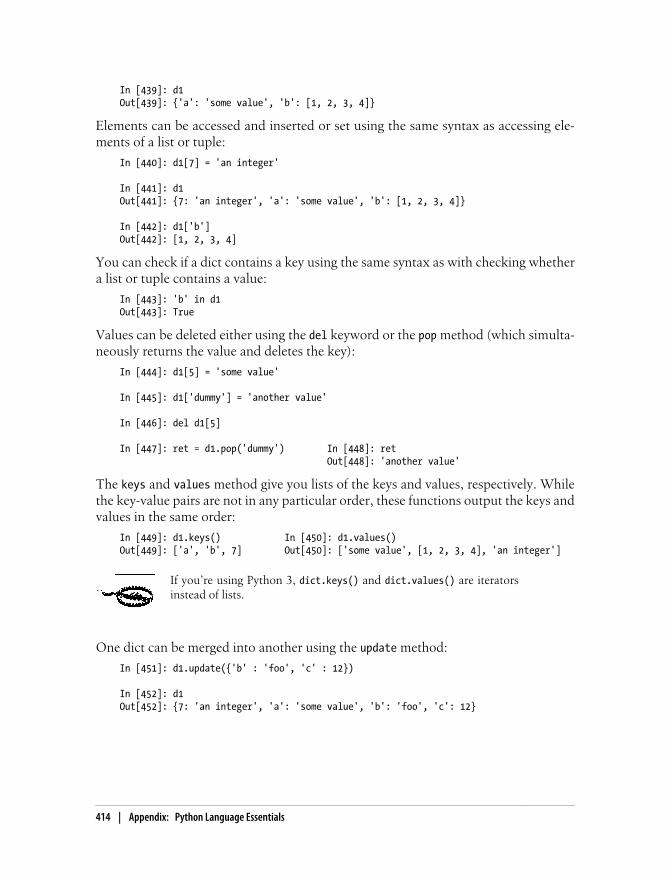
In [439]: d1Out[439]: {'a': 'some value', 'b': [1, 2, 3, 4]}
Elements can be accessed and inserted or set using the same syntax as accessing ele-ments of a list or tuple:
In [440]: d1[7] = 'an integer'
In [441]: d1Out[441]: {7: 'an integer', 'a': 'some value', 'b': [1, 2, 3, 4]}
In [442]: d1['b']Out[442]: [1, 2, 3, 4]
You can check if a dict contains a key using the same syntax as with checking whethera list or tuple contains a value:
In [443]: 'b' in d1Out[443]: True
Values can be deleted either using the del keyword or the pop method (which simulta-neously returns the value and deletes the key):
In [444]: d1[5] = 'some value'
In [445]: d1['dummy'] = 'another value'
In [446]: del d1[5]
In [447]: ret = d1.pop('dummy') In [448]: ret Out[448]: 'another value'
The keys and values method give you lists of the keys and values, respectively. Whilethe key-value pairs are not in any particular order, these functions output the keys andvalues in the same order:
In [449]: d1.keys() In [450]: d1.values() Out[449]: ['a', 'b', 7] Out[450]: ['some value', [1, 2, 3, 4], 'an integer']
If you’re using Python 3, dict.keys() and dict.values() are iteratorsinstead of lists.
One dict can be merged into another using the update method:
In [451]: d1.update({'b' : 'foo', 'c' : 12})
In [452]: d1Out[452]: {7: 'an integer', 'a': 'some value', 'b': 'foo', 'c': 12}
414 | Appendix: Python Language Essentials

Creating dicts from sequences
It’s common to occasionally end up with two sequences that you want to pair up ele-ment-wise in a dict. As a first cut, you might write code like this:
mapping = {}for key, value in zip(key_list, value_list): mapping[key] = value
Since a dict is essentially a collection of 2-tuples, it should be no shock that the dicttype function accepts a list of 2-tuples:
In [453]: mapping = dict(zip(range(5), reversed(range(5))))
In [454]: mappingOut[454]: {0: 4, 1: 3, 2: 2, 3: 1, 4: 0}
In a later section we’ll talk about dict comprehensions, another elegant way to constructdicts.
Default values
It’s very common to have logic like:
if key in some_dict: value = some_dict[key]else: value = default_value
Thus, the dict methods get and pop can take a default value to be returned, so that theabove if-else block can be written simply as:
value = some_dict.get(key, default_value)
get by default will return None if the key is not present, while pop will raise an exception.With setting values, a common case is for the values in a dict to be other collections,like lists. For example, you could imagine categorizing a list of words by their first lettersas a dict of lists:
In [455]: words = ['apple', 'bat', 'bar', 'atom', 'book']
In [456]: by_letter = {}
In [457]: for word in words: .....: letter = word[0] .....: if letter not in by_letter: .....: by_letter[letter] = [word] .....: else: .....: by_letter[letter].append(word) .....:
In [458]: by_letterOut[458]: {'a': ['apple', 'atom'], 'b': ['bat', 'bar', 'book']}
The setdefault dict method is for precisely this purpose. The if-else block above canbe rewritten as:
Data Structures and Sequences | 415

by_letter.setdefault(letter, []).append(word)
The built-in collections module has a useful class, defaultdict, which makes this eveneasier. One is created by passing a type or function for generating the default value foreach slot in the dict:
from collections import defaultdictby_letter = defaultdict(list)for word in words: by_letter[word[0]].append(word)
The initializer to defaultdict only needs to be a callable object (e.g. any function), notnecessarily a type. Thus, if you wanted the default value to be 4 you could pass afunction returning 4
counts = defaultdict(lambda: 4)
Valid dict key types
While the values of a dict can be any Python object, the keys have to be immutableobjects like scalar types (int, float, string) or tuples (all the objects in the tuple need tobe immutable, too). The technical term here is hashability. You can check whether anobject is hashable (can be used as a key in a dict) with the hash function:
In [459]: hash('string')Out[459]: -9167918882415130555
In [460]: hash((1, 2, (2, 3)))Out[460]: 1097636502276347782
In [461]: hash((1, 2, [2, 3])) # fails because lists are mutable---------------------------------------------------------------------------TypeError Traceback (most recent call last)<ipython-input-461-800cd14ba8be> in <module>()----> 1 hash((1, 2, [2, 3])) # fails because lists are mutableTypeError: unhashable type: 'list'
To use a list as a key, an easy fix is to convert it to a tuple:
In [462]: d = {}
In [463]: d[tuple([1, 2, 3])] = 5
In [464]: dOut[464]: {(1, 2, 3): 5}
SetA set is an unordered collection of unique elements. You can think of them like dicts,but keys only, no values. A set can be created in two ways: via the set function or usinga set literal with curly braces:
In [465]: set([2, 2, 2, 1, 3, 3])Out[465]: set([1, 2, 3])
416 | Appendix: Python Language Essentials
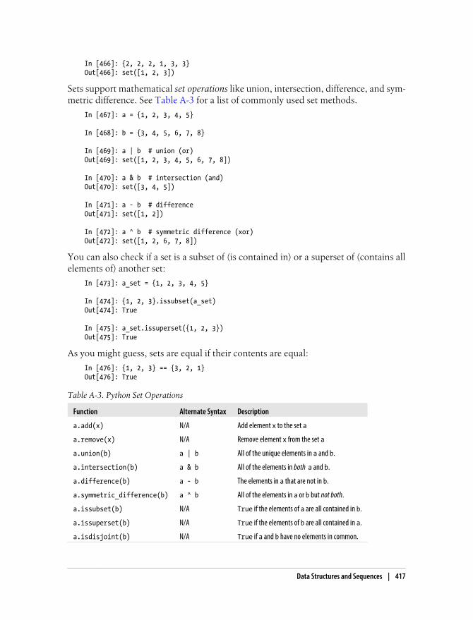
In [466]: {2, 2, 2, 1, 3, 3}Out[466]: set([1, 2, 3])
Sets support mathematical set operations like union, intersection, difference, and sym-metric difference. See Table A-3 for a list of commonly used set methods.
In [467]: a = {1, 2, 3, 4, 5}
In [468]: b = {3, 4, 5, 6, 7, 8}
In [469]: a | b # union (or)Out[469]: set([1, 2, 3, 4, 5, 6, 7, 8])
In [470]: a & b # intersection (and)Out[470]: set([3, 4, 5])
In [471]: a - b # differenceOut[471]: set([1, 2])
In [472]: a ^ b # symmetric difference (xor)Out[472]: set([1, 2, 6, 7, 8])
You can also check if a set is a subset of (is contained in) or a superset of (contains allelements of) another set:
In [473]: a_set = {1, 2, 3, 4, 5}
In [474]: {1, 2, 3}.issubset(a_set)Out[474]: True
In [475]: a_set.issuperset({1, 2, 3})Out[475]: True
As you might guess, sets are equal if their contents are equal:
In [476]: {1, 2, 3} == {3, 2, 1}Out[476]: True
Table A-3. Python Set Operations
Function Alternate Syntax Description
a.add(x) N/A Add element x to the set a
a.remove(x) N/A Remove element x from the set a
a.union(b) a | b All of the unique elements in a and b.
a.intersection(b) a & b All of the elements in both a and b.
a.difference(b) a - b The elements in a that are not in b.
a.symmetric_difference(b) a ^ b All of the elements in a or b but not both.
a.issubset(b) N/A True if the elements of a are all contained in b.
a.issuperset(b) N/A True if the elements of b are all contained in a.
a.isdisjoint(b) N/A True if a and b have no elements in common.
Data Structures and Sequences | 417
List, Set, and Dict ComprehensionsList comprehensions are one of the most-loved Python language features. They allowyou to concisely form a new list by filtering the elements of a collection and transformingthe elements passing the filter in one conscise expression. They take the basic form:
[expr for val in collection if condition]
This is equivalent to the following for loop:
result = []for val in collection: if condition: result.append(expr)
The filter condition can be omitted, leaving only the expression. For example, given alist of strings, we could filter out strings with length 2 or less and also convert them touppercase like this:
In [477]: strings = ['a', 'as', 'bat', 'car', 'dove', 'python']
In [478]: [x.upper() for x in strings if len(x) > 2]Out[478]: ['BAT', 'CAR', 'DOVE', 'PYTHON']
Set and dict comprehensions are a natural extension, producing sets and dicts in aidiomatically similar way instead of lists. A dict comprehension looks like this:
dict_comp = {key-expr : value-expr for value in collection if condition}
A set comprehension looks like the equivalent list comprehension except with curlybraces instead of square brackets:
set_comp = {expr for value in collection if condition}
Like list comprehensions, set and dict comprehensions are just syntactic sugar, but theysimilarly can make code both easier to write and read. Consider the list of strings above.Suppose we wanted a set containing just the lengths of the strings contained in thecollection; this could be easily computed using a set comprehension:
In [479]: unique_lengths = {len(x) for x in strings}
In [480]: unique_lengthsOut[480]: set([1, 2, 3, 4, 6])
As a simple dict comprehension example, we could create a lookup map of these stringsto their locations in the list:
In [481]: loc_mapping = {val : index for index, val in enumerate(strings)}
In [482]: loc_mappingOut[482]: {'a': 0, 'as': 1, 'bat': 2, 'car': 3, 'dove': 4, 'python': 5}
Note that this dict could be equivalently constructed by:
loc_mapping = dict((val, idx) for idx, val in enumerate(strings)}
418 | Appendix: Python Language Essentials

The dict comprehension version is shorter and cleaner in my opinion.
Dict and set comprehensions were added to Python fairly recently inPython 2.7 and Python 3.1+.
Nested list comprehensions
Suppose we have a list of lists containing some boy and girl names:
In [483]: all_data = [['Tom', 'Billy', 'Jefferson', 'Andrew', 'Wesley', 'Steven', 'Joe'], .....: ['Susie', 'Casey', 'Jill', 'Ana', 'Eva', 'Jennifer', 'Stephanie']]
You might have gotten these names from a couple of files and decided to keep the boyand girl names separate. Now, suppose we wanted to get a single list containing allnames with two or more e’s in them. We could certainly do this with a simple for loop:
names_of_interest = []for names in all_data: enough_es = [name for name in names if name.count('e') > 2] names_of_interest.extend(enough_es)
You can actually wrap this whole operation up in a single nested list comprehension,which will look like:
In [484]: result = [name for names in all_data for name in names .....: if name.count('e') >= 2]
In [485]: resultOut[485]: ['Jefferson', 'Wesley', 'Steven', 'Jennifer', 'Stephanie']
At first, nested list comprehensions are a bit hard to wrap your head around. The forparts of the list comprehension are arranged according to the order of nesting, and anyfilter condition is put at the end as before. Here is another example where we “flatten”a list of tuples of integers into a simple list of integers:
In [486]: some_tuples = [(1, 2, 3), (4, 5, 6), (7, 8, 9)]
In [487]: flattened = [x for tup in some_tuples for x in tup]
In [488]: flattenedOut[488]: [1, 2, 3, 4, 5, 6, 7, 8, 9]
Keep in mind that the order of the for expressions would be the same if you wrote anested for loop instead of a list comprehension:
flattened = []
for tup in some_tuples: for x in tup: flattened.append(x)
Data Structures and Sequences | 419

You can have arbitrarily many levels of nesting, though if you have more than two orthree levels of nesting you should probably start to question your data structure design.It’s important to distinguish the above syntax from a list comprehension inside a listcomprehension, which is also perfectly valid:
In [229]: [[x for x in tup] for tup in some_tuples]
FunctionsFunctions are the primary and most important method of code organization and reusein Python. There may not be such a thing as having too many functions. In fact, I wouldargue that most programmers doing data analysis don’t write enough functions! As youhave likely inferred from prior examples, functions are declared using the def keywordand returned from using the return keyword:
def my_function(x, y, z=1.5): if z > 1: return z * (x + y) else: return z / (x + y)
There is no issue with having multiple return statements. If the end of a function isreached without encountering a return statement, None is returned.
Each function can have some number of positional arguments and some number of keyword arguments. Keyword arguments are most commonly used to specify defaultvalues or optional arguments. In the above function, x and y are positional argumentswhile z is a keyword argument. This means that it can be called in either of theseequivalent ways:
my_function(5, 6, z=0.7)my_function(3.14, 7, 3.5)
The main restriction on function arguments it that the keyword arguments must followthe positional arguments (if any). You can specify keyword arguments in any order;this frees you from having to remember which order the function arguments werespecified in and only what their names are.
Namespaces, Scope, and Local FunctionsFunctions can access variables in two different scopes: global and local. An alternateand more descriptive name describing a variable scope in Python is a namespace. Anyvariables that are assigned within a function by default are assigned to the local name-space. The local namespace is created when the function is called and immediatelypopulated by the function’s arguments. After the function is finished, the local name-space is destroyed (with some exceptions, see section on closures below). Consider thefollowing function:
420 | Appendix: Python Language Essentials
def func(): a = [] for i in range(5): a.append(i)
Upon calling func(), the empty list a is created, 5 elements are appended, then a isdestroyed when the function exits. Suppose instead we had declared a
a = []def func(): for i in range(5): a.append(i)
Assigning global variables within a function is possible, but those variables must bedeclared as global using the global keyword:
In [489]: a = None
In [490]: def bind_a_variable(): .....: global a .....: a = [] .....: bind_a_variable() .....:
In [491]: print a[]
I generally discourage people from using the global keyword frequently.Typically global variables are used to store some kind of state in a sys-tem. If you find yourself using a lot of them, it’s probably a sign thatsome object-oriented programming (using classes) is in order.
Functions can be declared anywhere, and there is no problem with having local func-tions that are dynamically created when a function is called:
def outer_function(x, y, z): def inner_function(a, b, c): pass pass
In the above code, the inner_function will not exist until outer_function is called. Assoon as outer_function is done executing, the inner_function is destroyed.
Nested inner functions can access the local namespace of the enclosing function, butthey cannot bind new variables in it. I’ll talk a bit more about this in the section onclosures.
In a strict sense, all functions are local to some scope, that scope may just be the modulelevel scope.
Functions | 421

Returning Multiple ValuesWhen I first programmed in Python after having programmed in Java and C++, one ofmy favorite features was the ability to return multiple values from a function. Here’s asimple example:
def f(): a = 5 b = 6 c = 7 return a, b, c
a, b, c = f()
In data analysis and other scientific applications, you will likely find yourself doing thisvery often as many functions may have multiple outputs, whether those are data struc-tures or other auxiliary data computed inside the function. If you think about tuplepacking and unpacking from earlier in this chapter, you may realize that what’s hap-pening here is that the function is actually just returning one object, namely a tuple,which is then being unpacked into the result variables. In the above example, we couldhave done instead:
return_value = f()
In this case, return_value would be, as you may guess, a 3-tuple with the three returnedvariables. A potentially attractive alternative to returning multiple values like abovemight be to return a dict instead:
def f(): a = 5 b = 6 c = 7 return {'a' : a, 'b' : b, 'c' : c}
Functions Are ObjectsSince Python functions are objects, many constructs can be easily expressed that aredifficult to do in other languages. Suppose we were doing some data cleaning andneeded to apply a bunch of transformations to the following list of strings:
states = [' Alabama ', 'Georgia!', 'Georgia', 'georgia', 'FlOrIda', 'south carolina##', 'West virginia?']
Anyone who has ever worked with user-submitted survey data can expect messy resultslike these. Lots of things need to happen to make this list of strings uniform and readyfor analysis: whitespace stripping, removing punctuation symbols, and proper capital-ization. As a first pass, we might write some code like:
import re # Regular expression module
def clean_strings(strings): result = []
422 | Appendix: Python Language Essentials

for value in strings: value = value.strip() value = re.sub('[!#?]', '', value) # remove punctuation value = value.title() result.append(value) return result
The result looks like this:
In [15]: clean_strings(states)Out[15]:['Alabama', 'Georgia', 'Georgia', 'Georgia', 'Florida', 'South Carolina', 'West Virginia']
An alternate approach that you may find useful is to make a list of the operations youwant to apply to a particular set of strings:
def remove_punctuation(value): return re.sub('[!#?]', '', value)
clean_ops = [str.strip, remove_punctuation, str.title]
def clean_strings(strings, ops): result = [] for value in strings: for function in ops: value = function(value) result.append(value) return result
Then we have
In [22]: clean_strings(states, clean_ops)Out[22]:['Alabama', 'Georgia', 'Georgia', 'Georgia', 'Florida', 'South Carolina', 'West Virginia']
A more functional pattern like this enables you to easily modify how the strings aretransformed at a very high level. The clean_strings function is also now more reusable!
You can naturally use functions as arguments to other functions like the built-in mapfunction, which applies a function to a collection of some kind:
In [23]: map(remove_punctuation, states)Out[23]:[' Alabama ', 'Georgia',
Functions | 423

'Georgia', 'georgia', 'FlOrIda', 'south carolina', 'West virginia']
Anonymous (lambda) FunctionsPython has support for so-called anonymous or lambda functions, which are really justsimple functions consisting of a single statement, the result of which is the return value.They are defined using the lambda keyword, which has no meaning other than “we aredeclaring an anonymous function.”
def short_function(x): return x * 2
equiv_anon = lambda x: x * 2
I usually refer to these as lambda functions in the rest of the book. They are especiallyconvenient in data analysis because, as you’ll see, there are many cases where datatransformation functions will take functions as arguments. It’s often less typing (andclearer) to pass a lambda function as opposed to writing a full-out function declarationor even assigning the lambda function to a local variable. For example, consider thissilly example:
def apply_to_list(some_list, f): return [f(x) for x in some_list]
ints = [4, 0, 1, 5, 6]apply_to_list(ints, lambda x: x * 2)
You could also have written [x * 2 for x in ints], but here we were able to succintlypass a custom operator to the apply_to_list function.
As another example, suppose you wanted to sort a collection of strings by the numberof distinct letters in each string:
In [492]: strings = ['foo', 'card', 'bar', 'aaaa', 'abab']
Here we could pass a lambda function to the list’s sort method:
In [493]: strings.sort(key=lambda x: len(set(list(x))))
In [494]: stringsOut[494]: ['aaaa', 'foo', 'abab', 'bar', 'card']
One reason lambda functions are called anonymous functions is thatthe function object itself is never given a name attribute.
424 | Appendix: Python Language Essentials
Closures: Functions that Return FunctionsClosures are nothing to fear. They can actually be a very useful and powerful tool inthe right circumstance! In a nutshell, a closure is any dynamically-generated functionreturned by another function. The key property is that the returned function has accessto the variables in the local namespace where it was created. Here is a very simpleexample:
def make_closure(a): def closure(): print('I know the secret: %d' % a) return closure
closure = make_closure(5)
The difference between a closure and a regular Python function is that the closurecontinues to have access to the namespace (the function) where it was created, eventhough that function is done executing. So in the above case, the returned closure willalways print I know the secret: 5 whenever you call it. While it’s common to createclosures whose internal state (in this example, only the value of a) is static, you can justas easily have a mutable object like a dict, set, or list that can be modified. For example,here’s a function that returns a function that keeps track of arguments it has been calledwith:
def make_watcher(): have_seen = {}
def has_been_seen(x): if x in have_seen: return True else: have_seen[x] = True return False
return has_been_seen
Using this on a sequence of integers I obtain:
In [496]: watcher = make_watcher()
In [497]: vals = [5, 6, 1, 5, 1, 6, 3, 5]
In [498]: [watcher(x) for x in vals]Out[498]: [False, False, False, True, True, True, False, True]
However, one technical limitation to keep in mind is that while you can mutate anyinternal state objects (like adding key-value pairs to a dict), you cannot bind variablesin the enclosing function scope. One way to work around this is to modify a dict or listrather than binding variables:
def make_counter(): count = [0] def counter():
Functions | 425

# increment and return the current count count[0] += 1 return count[0] return counter
counter = make_counter()
You might be wondering why this is useful. In practice, you can write very generalfunctions with lots of options, then fabricate simpler, more specialized functions.Here’s an example of creating a string formatting function:
def format_and_pad(template, space): def formatter(x): return (template % x).rjust(space)
return formatter
You could then create a floating point formatter that always returns a length-15 stringlike so:
In [500]: fmt = format_and_pad('%.4f', 15)
In [501]: fmt(1.756)Out[501]: ' 1.7560'
If you learn more about object-oriented programming in Python, you might observethat these patterns also could be implemented (albeit more verbosely) using classes.
Extended Call Syntax with *args, **kwargsThe way that function arguments work under the hood in Python is actually very sim-ple. When you write func(a, b, c, d=some, e=value), the positional and keywordarguments are actually packed up into a tuple and dict, respectively. So the internalfunction receives a tuple args and dict kwargs and internally does the equivalent of:
a, b, c = argsd = kwargs.get('d', d_default_value)e = kwargs.get('e', e_default_value)
This all happens nicely behind the scenes. Of course, it also does some error checkingand allows you to specify some of the positional arguments as keywords also (even ifthey aren’t keyword in the function declaration!).
def say_hello_then_call_f(f, *args, **kwargs): print 'args is', args print 'kwargs is', kwargs print("Hello! Now I'm going to call %s" % f) return f(*args, **kwargs)
def g(x, y, z=1): return (x + y) / z
Then if we call g with say_hello_then_call_f we get:
426 | Appendix: Python Language Essentials

In [8]: say_hello_then_call_f(g, 1, 2, z=5.)args is (1, 2)kwargs is {'z': 5.0}Hello! Now I'm going to call <function g at 0x2dd5cf8>Out[8]: 0.6
Currying: Partial Argument ApplicationCurrying is a fun computer science term which means deriving new functions fromexisting ones by partial argument application. For example, suppose we had a trivialfunction that adds two numbers together:
def add_numbers(x, y): return x + y
Using this function, we could derive a new function of one variable, add_five, that adds5 to its argument:
add_five = lambda y: add_numbers(5, y)
The second argument to add_numbers is said to be curried. There’s nothing very fancyhere as we really only have defined a new function that calls an existing function. Thebuilt-in functools module can simplify this process using the partial function:
from functools import partialadd_five = partial(add_numbers, 5)
When discussing pandas and time series data, we’ll use this technique to create speci-alized functions for transforming data series
# compute 60-day moving average of time series xma60 = lambda x: pandas.rolling_mean(x, 60)
# Take the 60-day moving average of of all time series in datadata.apply(ma60)
GeneratorsHaving a consistent way to iterate over sequences, like objects in a list or lines in a file,is an important Python feature. This is accomplished by means of the iterator proto-col, a generic way to make objects iterable. For example, iterating over a dict yields thedict keys:
In [502]: some_dict = {'a': 1, 'b': 2, 'c': 3}
In [503]: for key in some_dict: .....: print key,a c b
When you write for key in some_dict, the Python interpreter first attempts to createan iterator out of some_dict:
In [504]: dict_iterator = iter(some_dict)
Functions | 427
In [505]: dict_iteratorOut[505]: <dictionary-keyiterator at 0x10a0a1578>
Any iterator is any object that will yield objects to the Python interpreter when used ina context like a for loop. Most methods expecting a list or list-like object will also acceptany iterable object. This includes built-in methods such as min, max, and sum, and typeconstructors like list and tuple:
In [506]: list(dict_iterator)Out[506]: ['a', 'c', 'b']
A generator is a simple way to construct a new iterable object. Whereas normal func-tions execute and return a single value, generators return a sequence of values lazily,pausing after each one until the next one is requested. To create a generator, use theyield keyword instead of return in a function:
def squares(n=10): for i in xrange(1, n + 1): print 'Generating squares from 1 to %d' % (n ** 2) yield i ** 2
When you actually call the generator, no code is immediately executed:
In [2]: gen = squares()
In [3]: genOut[3]: <generator object squares at 0x34c8280>
It is not until you request elements from the generator that it begins executing its code:
In [4]: for x in gen: ...: print x, ...:Generating squares from 0 to 1001 4 9 16 25 36 49 64 81 100
As a less trivial example, suppose we wished to find all unique ways to make changefor $1 (100 cents) using an arbitrary set of coins. You can probably think of variousways to implement this and how to store the unique combinations as you come up withthem. One way is to write a generator that yields lists of coins (represented as integers):
def make_change(amount, coins=[1, 5, 10, 25], hand=None): hand = [] if hand is None else hand if amount == 0: yield hand for coin in coins: # ensures we don't give too much change, and combinations are unique if coin > amount or (len(hand) > 0 and hand[-1] < coin): continue
for result in make_change(amount - coin, coins=coins, hand=hand + [coin]): yield result
The details of the algorithm are not that important (can you think of a shorter way?).Then we can write:
428 | Appendix: Python Language Essentials

In [508]: for way in make_change(100, coins=[10, 25, 50]): .....: print way[10, 10, 10, 10, 10, 10, 10, 10, 10, 10][25, 25, 10, 10, 10, 10, 10][25, 25, 25, 25][50, 10, 10, 10, 10, 10][50, 25, 25][50, 50]
In [509]: len(list(make_change(100)))Out[509]: 242
Generator expresssions
A simple way to make a generator is by using a generator expression. This is a generatoranalogue to list, dict and set comprehensions; to create one, enclose what would other-wise be a list comprehension with parenthesis instead of brackets:
In [510]: gen = (x ** 2 for x in xrange(100))
In [511]: genOut[511]: <generator object <genexpr> at 0x10a0a31e0>
This is completely equivalent to the following more verbose generator:
def _make_gen(): for x in xrange(100): yield x ** 2gen = _make_gen()
Generator expressions can be used inside any Python function that will accept a gen-erator:
In [512]: sum(x ** 2 for x in xrange(100))Out[512]: 328350
In [513]: dict((i, i **2) for i in xrange(5))Out[513]: {0: 0, 1: 1, 2: 4, 3: 9, 4: 16}
itertools module
The standard library itertools module has a collection of generators for many commondata algorithms. For example, groupby takes any sequence and a function; this groupsconsecutive elements in the sequence by return value of the function. Here’s an exam-ple:
In [514]: import itertools
In [515]: first_letter = lambda x: x[0]
In [516]: names = ['Alan', 'Adam', 'Wes', 'Will', 'Albert', 'Steven']
In [517]: for letter, names in itertools.groupby(names, first_letter): .....: print letter, list(names) # names is a generatorA ['Alan', 'Adam']
Functions | 429
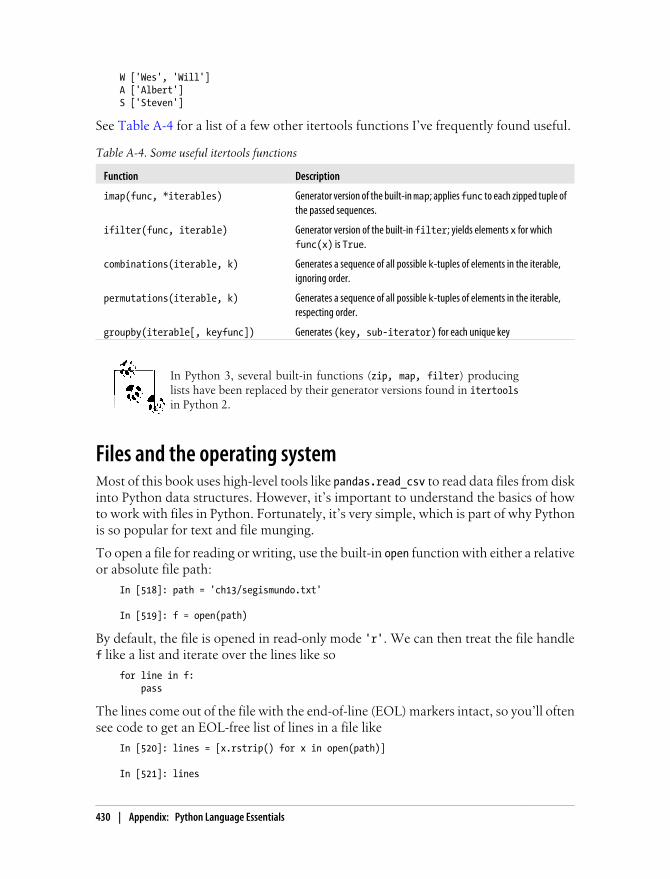
W ['Wes', 'Will']A ['Albert']S ['Steven']
See Table A-4 for a list of a few other itertools functions I’ve frequently found useful.
Table A-4. Some useful itertools functions
Function Description
imap(func, *iterables) Generator version of the built-in map; applies func to each zipped tuple ofthe passed sequences.
ifilter(func, iterable) Generator version of the built-in filter; yields elements x for whichfunc(x) is True.
combinations(iterable, k) Generates a sequence of all possible k-tuples of elements in the iterable,ignoring order.
permutations(iterable, k) Generates a sequence of all possible k-tuples of elements in the iterable,respecting order.
groupby(iterable[, keyfunc]) Generates (key, sub-iterator) for each unique key
In Python 3, several built-in functions (zip, map, filter) producinglists have been replaced by their generator versions found in itertoolsin Python 2.
Files and the operating systemMost of this book uses high-level tools like pandas.read_csv to read data files from diskinto Python data structures. However, it’s important to understand the basics of howto work with files in Python. Fortunately, it’s very simple, which is part of why Pythonis so popular for text and file munging.
To open a file for reading or writing, use the built-in open function with either a relativeor absolute file path:
In [518]: path = 'ch13/segismundo.txt'
In [519]: f = open(path)
By default, the file is opened in read-only mode 'r'. We can then treat the file handlef like a list and iterate over the lines like so
for line in f: pass
The lines come out of the file with the end-of-line (EOL) markers intact, so you’ll oftensee code to get an EOL-free list of lines in a file like
In [520]: lines = [x.rstrip() for x in open(path)]
In [521]: lines
430 | Appendix: Python Language Essentials
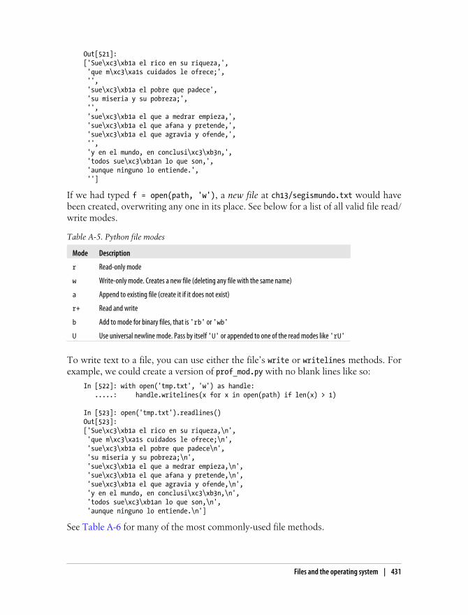
Out[521]: ['Sue\xc3\xb1a el rico en su riqueza,', 'que m\xc3\xa1s cuidados le ofrece;', '', 'sue\xc3\xb1a el pobre que padece', 'su miseria y su pobreza;', '', 'sue\xc3\xb1a el que a medrar empieza,', 'sue\xc3\xb1a el que afana y pretende,', 'sue\xc3\xb1a el que agravia y ofende,', '', 'y en el mundo, en conclusi\xc3\xb3n,', 'todos sue\xc3\xb1an lo que son,', 'aunque ninguno lo entiende.', '']
If we had typed f = open(path, 'w'), a new file at ch13/segismundo.txt would havebeen created, overwriting any one in its place. See below for a list of all valid file read/write modes.
Table A-5. Python file modes
Mode Description
r Read-only mode
w Write-only mode. Creates a new file (deleting any file with the same name)
a Append to existing file (create it if it does not exist)
r+ Read and write
b Add to mode for binary files, that is 'rb' or 'wb'
U Use universal newline mode. Pass by itself 'U' or appended to one of the read modes like 'rU'
To write text to a file, you can use either the file’s write or writelines methods. Forexample, we could create a version of prof_mod.py with no blank lines like so:
In [522]: with open('tmp.txt', 'w') as handle: .....: handle.writelines(x for x in open(path) if len(x) > 1)
In [523]: open('tmp.txt').readlines()Out[523]: ['Sue\xc3\xb1a el rico en su riqueza,\n', 'que m\xc3\xa1s cuidados le ofrece;\n', 'sue\xc3\xb1a el pobre que padece\n', 'su miseria y su pobreza;\n', 'sue\xc3\xb1a el que a medrar empieza,\n', 'sue\xc3\xb1a el que afana y pretende,\n', 'sue\xc3\xb1a el que agravia y ofende,\n', 'y en el mundo, en conclusi\xc3\xb3n,\n', 'todos sue\xc3\xb1an lo que son,\n', 'aunque ninguno lo entiende.\n']
See Table A-6 for many of the most commonly-used file methods.
Files and the operating system | 431

Table A-6. Important Python file methods or attributes
Method Description
read([size]) Return data from file as a string, with optional size argument indicating the number of bytesto read
readlines([size]) Return list of lines in the file, with optional size argument
readlines([size]) Return list of lines (as strings) in the file
write(str) Write passed string to file.
writelines(strings) Write passed sequence of strings to the file.
close() Close the handle
flush() Flush the internal I/O buffer to disk
seek(pos) Move to indicated file position (integer).
tell() Return current file position as integer.
closed True is the file is closed.
432 | Appendix: Python Language Essentials

Index
Symbols! character, 60, 61, 64!= operator, 91!cmd command, 60"two-language" problem, 2–3# (hash mark), 388$PATH variable, 10% character, 398%a datetime format, 293%A datetime format, 293%alias magic function, 61%automagic magic function, 55%b datetime format, 293%B datetime format, 293%bookmark magic function, 60, 62%c datetime format, 293%cd magic function, 60%cpaste magic function, 51–52, 55%d datetime format, 292%D datetime format, 293%d format character, 398%debug magic function, 54–55, 62%dhist magic function, 60%dirs magic function, 60%env magic function, 60%F datetime format, 293%gui magic function, 57%H datetime format, 292%hist magic function, 55, 59%I datetime format, 292%logstart magic function, 60%logstop magic function, 60%lprun magic function, 70, 72%m datetime format, 292
%M datetime format, 292%magic magic function, 55%p datetime format, 293%page magic function, 55%paste magic function, 51, 55%pdb magic function, 54, 63%popd magic function, 60%prun magic function, 55, 70%pushd magic function, 60%pwd magic function, 60%quickref magic function, 55%reset magic function, 55, 59%run magic function, 49–50, 55, 386%S datetime format, 292%s format character, 398%time magic function, 55, 67%timeit magic function, 54, 67, 68%U datetime format, 293%w datetime format, 292%W datetime format, 293%who magic function, 55%whos magic function, 55%who_ls magic function, 55%x datetime format, 293%X datetime format, 293%xdel magic function, 55, 59%xmode magic function, 54%Y datetime format, 292%y datetime format, 292%z datetime format, 293& operator, 91* operator, 105+ operator, 406, 4092012 Federal Election Commission database
example, 278–287
We’d like to hear your suggestions for improving our indexes. Send email to [email protected].
433
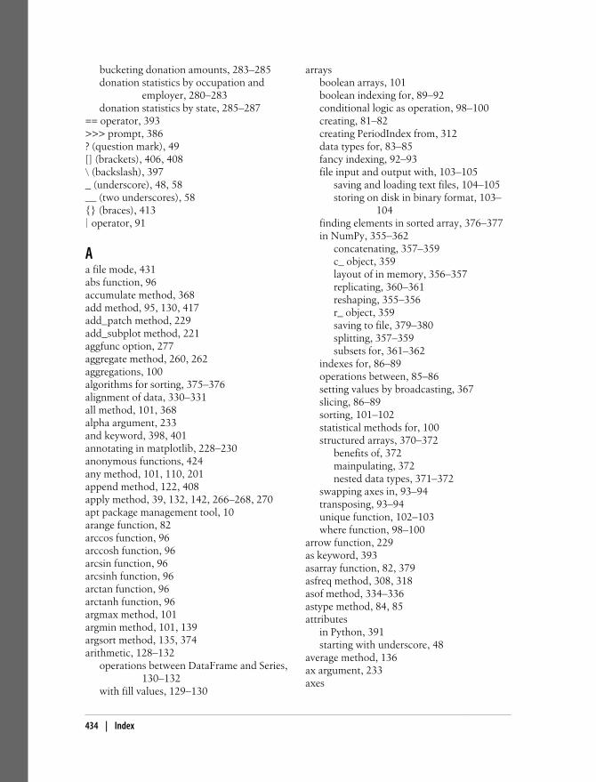
bucketing donation amounts, 283–285donation statistics by occupation and
employer, 280–283donation statistics by state, 285–287
== operator, 393>>> prompt, 386? (question mark), 49[] (brackets), 406, 408\ (backslash), 397_ (underscore), 48, 58__ (two underscores), 58{} (braces), 413| operator, 91
Aa file mode, 431abs function, 96accumulate method, 368add method, 95, 130, 417add_patch method, 229add_subplot method, 221aggfunc option, 277aggregate method, 260, 262aggregations, 100algorithms for sorting, 375–376alignment of data, 330–331all method, 101, 368alpha argument, 233and keyword, 398, 401annotating in matplotlib, 228–230anonymous functions, 424any method, 101, 110, 201append method, 122, 408apply method, 39, 132, 142, 266–268, 270apt package management tool, 10arange function, 82arccos function, 96arccosh function, 96arcsin function, 96arcsinh function, 96arctan function, 96arctanh function, 96argmax method, 101argmin method, 101, 139argsort method, 135, 374arithmetic, 128–132
operations between DataFrame and Series,130–132
with fill values, 129–130
arraysboolean arrays, 101boolean indexing for, 89–92conditional logic as operation, 98–100creating, 81–82creating PeriodIndex from, 312data types for, 83–85fancy indexing, 92–93file input and output with, 103–105
saving and loading text files, 104–105storing on disk in binary format, 103–
104finding elements in sorted array, 376–377in NumPy, 355–362
concatenating, 357–359c_ object, 359layout of in memory, 356–357replicating, 360–361reshaping, 355–356r_ object, 359saving to file, 379–380splitting, 357–359subsets for, 361–362
indexes for, 86–89operations between, 85–86setting values by broadcasting, 367slicing, 86–89sorting, 101–102statistical methods for, 100structured arrays, 370–372
benefits of, 372mainpulating, 372nested data types, 371–372
swapping axes in, 93–94transposing, 93–94unique function, 102–103where function, 98–100
arrow function, 229as keyword, 393asarray function, 82, 379asfreq method, 308, 318asof method, 334–336astype method, 84, 85attributes
in Python, 391starting with underscore, 48
average method, 136ax argument, 233axes
434 | Index

broadcasting over, 364–367concatenating along, 185–188labels for, 226–227renaming indexes for, 197–198swapping in arrays, 93–94
AxesSubplot object, 221axis argument, 188axis method, 138
Bb file mode, 431backslash (\), 397bar plots, 235–238Basemap object, 245, 246.bashrc file, 10.bash_profile file, 9bbox_inches option, 231benefits
of Python, 2–3glue for code, 2solving "two-language" problem with, 2–
3of structured arrays, 372
beta function, 107defined, 342
between_time method, 335bfill method, 123bin edges, 314binary data formats, 171–172
HDF5, 171–172Microsoft Excel files, 172storing arrays in, 103–104
binary moving window functions, 324–325binary search of lists, 410binary universal functions, 96binding
defined, 390variables, 425
binomial function, 107bisect module, 410bookmarking directories in IPython, 62Boolean
arrays, 101data type, 84, 398indexing for arrays, 89–92
bottleneck library, 324braces ({}), 413brackets ([]), 406, 408break keyword, 401
broadcasting, 362–367defined, 86, 360, 362over other axes, 364–367setting array values by, 367
bucketing, 283–285
Ccalendar module, 290casting, 84cat method, 156, 212Categorical object, 199ceil function, 96center method, 212Chaco, 248chisquare function, 107chunksize argument, 160, 161clearing screen shortcut, 53clipboard, executing code from, 50–52clock function, 67close method, 220, 432closures, 425–426cmd.exe, 7collections module, 416colons, 387cols option, 277columns, grouping on, 256–257column_stack function, 359combinations function, 430combine_first method, 177, 189combining
data sources, 336–338data sources, with overlap, 188–189lists, 409
commands, 65(see also magic commands)debugger, 65history in IPython, 58–60
input and output variables, 58–59logging of, 59–60reusing command history, 58
searching for, 53comment argument, 160comments in Python, 388compile method, 208complex128 data type, 84complex256 data type, 84complex64 data type, 84concat function, 34, 177, 184, 185, 186, 267,
357, 359
Index | 435

concatenatingalong axis, 185–188arrays, 357–359
conditional logic as array operation, 98–100conferences, 12configuring matplotlib, 231–232conforming, 122contains method, 212contiguous memory, 381–382continue keyword, 401continuous return, 348convention argument, 314converting
between string and datetime, 291–293timestamps to periods, 311
coordinated universal time (UTC), 303copy argument, 181copy method, 118copysign function, 96corr method, 140correlation, 139–141corrwith method, 140cos function, 96cosh function, 96count method, 139, 206, 212, 261, 407Counter class, 21cov method, 140covariance, 139–141CPython, 7cross-section, 329crosstab function, 277–278crowdsourcing, 241CSV files, 163–165, 242Ctrl-A keyboard shortcut, 53Ctrl-B keyboard shortcut, 53Ctrl-C keyboard shortcut, 53Ctrl-E keyboard shortcut, 53Ctrl-F keyboard shortcut, 53Ctrl-K keyboard shortcut, 53Ctrl-L keyboard shortcut, 53Ctrl-N keyboard shortcut, 53Ctrl-P keyboard shortcut, 53Ctrl-R keyboard shortcut, 53Ctrl-Shift-V keyboard shortcut, 53Ctrl-U keyboard shortcut, 53cummax method, 139cummin method, 139cumprod method, 100, 139cumsum method, 100, 139
cumulative returns, 338–340currying, 427cursor, moving with keyboard, 53custom universal functions, 370cut function, 199, 200, 201, 268, 283Cython project, 2, 382–383c_ object, 359
Ddata aggregation, 259–264
returning data in unindexed form, 264using multiple functions, 262–264
data alignment, 128–132arithmetic methods with fill values, 129–
130operations between DataFrame and Series,
130–132data munging, 329–340
asof method, 334–336combining data, 336–338for data alignment, 330–331for specialized frequencies, 332–334
data structures for pandas, 112–121DataFrame, 115–120Index objects, 120–121Panel, 152–154Series, 112–115
data typesfor arrays, 83–85for ndarray, 83–85for NumPy, 353–354
hierarchy of, 354for Python, 395–400
boolean data type, 398dates and times, 399–400None data type, 399numeric data types, 395–396str data type, 396–398type casting in, 399
for time series data, 290–293converting between string and datetime,
291–293nested, 371–372
data wranglingmanipulating strings, 205–211
methods for, 206–207vectorized string methods, 210–211with regular expressions, 207–210
merging data, 177–189
436 | Index
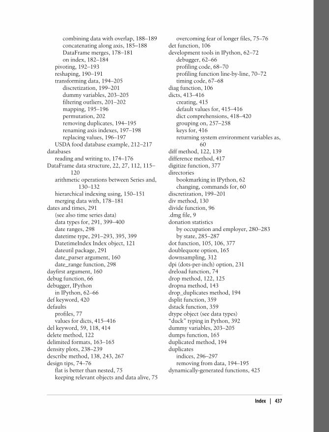
combining data with overlap, 188–189concatenating along axis, 185–188DataFrame merges, 178–181on index, 182–184
pivoting, 192–193reshaping, 190–191transforming data, 194–205
discretization, 199–201dummy variables, 203–205filtering outliers, 201–202mapping, 195–196permutation, 202removing duplicates, 194–195renaming axis indexes, 197–198replacing values, 196–197
USDA food database example, 212–217databases
reading and writing to, 174–176DataFrame data structure, 22, 27, 112, 115–
120arithmetic operations between Series and,
130–132hierarchical indexing using, 150–151merging data with, 178–181
dates and times, 291(see also time series data)data types for, 291, 399–400date ranges, 298datetime type, 291–293, 395, 399DatetimeIndex Index object, 121dateutil package, 291date_parser argument, 160date_range function, 298
dayfirst argument, 160debug function, 66debugger, IPython
in IPython, 62–66def keyword, 420defaults
profiles, 77values for dicts, 415–416
del keyword, 59, 118, 414delete method, 122delimited formats, 163–165density plots, 238–239describe method, 138, 243, 267design tips, 74–76
flat is better than nested, 75keeping relevant objects and data alive, 75
overcoming fear of longer files, 75–76det function, 106development tools in IPython, 62–72
debugger, 62–66profiling code, 68–70profiling function line-by-line, 70–72timing code, 67–68
diag function, 106dicts, 413–416
creating, 415default values for, 415–416dict comprehensions, 418–420grouping on, 257–258keys for, 416returning system environment variables as,
60diff method, 122, 139difference method, 417digitize function, 377directories
bookmarking in IPython, 62changing, commands for, 60
discretization, 199–201div method, 130divide function, 96.dmg file, 9donation statistics
by occupation and employer, 280–283by state, 285–287
dot function, 105, 106, 377doublequote option, 165downsampling, 312dpi (dots-per-inch) option, 231dreload function, 74drop method, 122, 125dropna method, 143drop_duplicates method, 194dsplit function, 359dstack function, 359dtype object (see data types)“duck” typing in Python, 392dummy variables, 203–205dumps function, 165duplicated method, 194duplicates
indices, 296–297removing from data, 194–195
dynamically-generated functions, 425
Index | 437

Eedgecolo option, 231edit-compile-run workflow, 45eig function, 106elif blocks (see if statements)else block (see if statements)empty function, 82, 83empty namespace, 50encoding argument, 160endswith method, 207, 212enumerate function, 412environment variables, 8, 60EPD (Enthought Python Distribution), 7–9equal function, 96escapechar option, 165ewma function, 323ewmcorr function, 323ewmcov function, 323ewmstd function, 323ewmvar function, 323ExcelFile class, 172except block, 403exceptions
automatically entering debugger after, 55defined, 402handling in Python, 402–404
exec keyword, 59execute-explore workflow, 45execution time
of code, 55of single statement, 55
exit command, 386exp function, 96expanding window mean, 322exponentially-weighted functions, 324extend method, 409extensible markup language (XML) files, 169–
170eye function, 83
Ffabs function, 96facecolor option, 231factor analysis, 342–343Factor object, 269factors, 342fancy indexing
defined, 361
for arrays, 92–93ffill method, 123figsize argument, 234Figure object, 220, 223file input/output
binary data formats for, 171–172HDF5, 171–172Microsoft Excel files, 172
for arrays, 103–105HDF5, 380memory-mapped files, 379–380saving and loading text files, 104–105storing on disk in binary format, 103–
104in Python, 430–431saving plot to file, 231text files, 155–170
delimited formats, 163–165HTML files, 166–170JSON data, 165–166lxml library, 166–170reading in pieces, 160–162writing to, 162–163XML files, 169–170
with databases, 174–176with Web APIs, 173–174
filling in missing data, 145–146, 270–271fillna method, 22, 143, 145, 146, 196, 270,
317fill_method argument, 313fill_value option, 277filtering
in pandas, 125–128missing data, 143–144outliers, 201–202
financial applicationscumulative returns, 338–340data munging, 329–340
asof method, 334–336combining data, 336–338for data alignment, 330–331for specialized frequencies, 332–334
future contract rolling, 347–350grouping for, 340–345
factor analysis with, 342–343quartile analysis, 343–345
linear regression, 350–351return indexes, 338–340rolling correlation, 350–351
438 | Index
signal frontier analysis, 345–347find method, 206, 207findall method, 167, 208, 210, 212finditer method, 210first crossing time, 109first method, 136, 261flat is better than nested, 75flattening, 356float data type, 83, 354, 395, 396, 399float function, 402float128 data type, 84float16 data type, 84float32 data type, 84float64 data type, 84floor function, 96floor_divide function, 96flow control, 400–405
exception handling, 402–404for loops, 401–402if statements, 400–401pass statements, 402range function, 404–405ternary expressions, 405while loops, 402xrange function, 404–405
flush method, 432fmax function, 96fmin function, 96fname option, 231for loops, 85, 100, 401–402, 418, 419format option, 231frequencies, 299–301
converting, 308specialized frequencies, 332–334week of month dates, 301
frompyfunc function, 370from_csv method, 163functions, 389, 420–430
anonymous functions, 424are objects, 422–423closures, 425–426currying of, 427extended call syntax for, 426lambda functions, 424namespaces for, 420–421parsing in pandas, 155returning multiple values from, 422scope of, 420–421
functools module, 427
future contract rolling, 347–350futures, 347
Ggamma function, 107gcc command, 9, 11generators, 427–430
defined, 428generator expressions, 429itertools module for, 429–430
get method, 167, 172, 212, 415getattr function, 391get_chunk method, 162get_dummies function, 203, 205get_value method, 128get_xlim method, 226GIL (global interpreter lock), 3global scope, 420, 421glue for code
Python as, 2.gov domain, 17Granger, Brian, 72graphics
Chaco, 248mayavi, 248
greater function, 96greater_equal function, 96grid argument, 234group keys, 268groupby method, 39, 252–259, 297, 316, 343,
377, 429iterating over groups, 255–256on column, 256–257on dict, 257–258on levels, 259resampling with, 316using functions with, 258–259with Series, 257–258
grouping2012 Federal Election Commission database
example, 278–287bucketing donation amounts, 283–285donation statistics by occupation and
employer, 280–283donation statistics by state, 285–287
apply method, 266–268data aggregation, 259–264
returning data in unindexed form, 264using multiple functions, 262–264
Index | 439

filling missing values with group-specificvalues, 270–271
for financial applications, 340–345factor analysis with, 342–343quartile analysis, 343–345
group weighted average, 273–274groupby method, 252–259
iterating over groups, 255–256on column, 256–257on dict, 257–258on levels, 259using functions with, 258–259with Series, 257–258
linear regression for, 274–275pivot tables, 275–278
cross-tabulation, 277–278quantile analysis with, 268–269random sampling with, 271–272
HHaiti earthquake crisis data example, 241–247half-open, 314hasattr function, 391hash mark (#), 388hashability, 416HDF5 (hierarchical data format), 171–172,
380HDFStore class, 171header argument, 160heapsort sorting method, 376hierarchical data format (HDF5), 171–172,
380hierarchical indexing
in pandas, 147–151sorting levels, 149–150summary statistics by level, 150with DataFrame columns, 150–151
reshaping data with, 190–191hist method, 238histograms, 238–239history of commands, searching, 53homogeneous data container, 370how argument, 181, 313, 316hsplit function, 359hstack function, 358HTML files, 166–170HTML Notebook in IPython, 72Hunter, John D., 5, 219hyperbolic trigonometric functions, 96
Iicol method, 128, 152IDEs (Integrated Development Environments),
11, 52idxmax method, 138idxmin method, 138if statements, 400–401, 415ifilter function, 430iget_value method, 152ignore_index argument, 188imap function, 430import directive
in Python, 392–393usage of in this book, 13
imshow function, 98in keyword, 409in-place sort, 373in1d method, 103indentation
in Python, 387–388IndentationError event, 51
index method, 206, 207Index objects data structure, 120–121indexes
defined, 112for arrays, 86–89for axis, 197–198for TimeSeries class, 294–296hierarchical indexing, 147–151
reshaping data with, 190–191sorting levels, 149–150summary statistics by level, 150with DataFrame columns, 150–151
in pandas, 136integer indexing, 151–152merging data on, 182–184
index_col argument, 160indirect sorts, 374–375, 374input variables, 58–59insert method, 122, 408insort method, 410int data type, 83, 395, 399int16 data type, 84int32 data type, 84int64 data type, 84Int64Index Index object, 121int8 data type, 84integer arrays, indexing using (see fancy
indexing)
440 | Index

integer indexing, 151–152Integrated Development Environments (IDEs),
11, 52interpreted languages
defined, 386Python interpreter, 386
interrupting code, 50, 53intersect1d method, 103intersection method, 122, 417intervals of time, 289inv function, 106inverse trigonometric functions, 96.ipynb files, 72IPython, 5
bookmarking directories, 62command history in, 58–60
input and output variables, 58–59logging of, 59–60reusing command history, 58
design tips, 74–76flat is better than nested, 75keeping relevant objects and data alive,
75overcoming fear of longer files, 75–76
development tools, 62–72debugger, 62–66profiling code, 68–70profiling function line-by-line, 70–72timing code, 67–68
executing code from clipboard, 50–52HTML Notebook in, 72integration with IDEs and editors, 52integration with mathplotlib, 56–57keyboard shortcuts for, 52magic commands in, 54–55making classes output correctly, 76object introspection in, 48–49profiles for, 77–78Qt console for, 55Quick Reference Card for, 55reloading module dependencies, 74%run command in, 49–50shell commands in, 60–61tab completion in, 47–48tracebacks in, 53–54
ipython_config.py file, 77irow method, 128, 152is keyword, 393isdisjoint method, 417
isfinite function, 96isin method, 141–142isinf function, 96isinstance function, 391isnull method, 96, 114, 143issubdtype function, 354issubset method, 417issuperset method, 417is_monotonic method, 122is_unique method, 122iter function, 392iterating over groups, 255–256iterator argument, 160iterator protocol, 392, 427itertools module, 429–430, 429ix_ function, 93
Jjoin method, 184, 206, 212JSON (JavaScript Object Notation), 18, 165–
166, 213
KKDE (kernel density estimate) plots, 239keep_date_col argument, 160kernels, 239key-value pairs, 413keyboard shortcuts, 53
for deleting text, 53for IPython, 52
KeyboardInterrupt event, 50keys
argument, 188for dicts, 416method, 414
keyword arguments, 389, 420kind argument, 234, 314kurt method, 139
Llabel argument, 233, 313, 315lambda functions, 211, 262, 424last method, 261layout of arrays in memory, 356–357left argument, 181left_index argument, 181left_on argument, 181legends in matplotlib, 228
Index | 441

len function, 212, 258less function, 96less_equal function, 96level keyword, 259levels
defined, 147grouping on, 259sorting, 149–150summary statistics by, 150
lexicographical sortdefined, 375lexsort method, 374
libraries, 3–6IPython, 5matplotlib, 5NumPy, 4pandas, 4–5SciPy, 6
limit argument, 313linalg function, 105line plots, 232–235linear algebra, 105–106linear regression, 274–275, 350–351lineterminator option, 164line_profiler extension, 70Linux, setting up on, 10–11list comprehensions, 418–420
nested list comprehensions, 419–420list function, 408lists, 408–411
adding elements to, 408–409binary search of, 410combining, 409insertion into sorted, 410list comprehensions, 418–420removing elements from, 408–409slicing, 410–411sorting, 409–410
ljust method, 207load function, 103, 379load method, 171loads function, 18local scope, 420localizing time series data, 304–305loffset argument, 313, 316log function, 96log1p function, 96log2 function, 96logging command history in IPython, 59–60
logical_and function, 96logical_not function, 96logical_or function, 96logical_xor function, 96logy argument, 234long format, 192long type, 395longer files overcoming fear of, 75–76lower method, 207, 212lstrip method, 207, 212lstsq function, 106lxml library, 166–170
Mmad method, 139magic methods, 48, 54–55main function, 75mainpulating structured arrays, 372many-to-many merge, 179many-to-one merge, 178map method, 133, 195–196, 211, 280, 423margins, 275markers, 224match method, 208–212matplotlib, 5, 219–232
annotating in, 228–230axis labels in, 226–227configuring, 231–232integrating with IPython, 56–57legends in, 228saving to file, 231styling for, 224–225subplots in, 220–224ticks in, 226–227title in, 226–227
matplotlibrc file, 232matrix operations in NumPy, 377–379max method, 101, 136, 139, 261, 428maximum function, 95, 96mayavi, 248mean method, 100, 139, 253, 259, 261, 265median method, 139, 261memmap object, 379memory, layout of arrays in, 356–357memory-mapped files
defined, 379saving arrays to file, 379–380
mergesort sorting method, 375, 376merging data, 177–189
442 | Index
combining data with overlap, 188–189concatenating along axis, 185–188DataFrame merges, 178–181on index, 182–184
meshgrid function, 97methods
defined, 389for tuples, 407in Python, 389starting with underscore, 48
Microsoft Excel files, 172.mil domain, 17min method, 101, 136, 139, 261, 428minimum function, 96missing data, 142–146
filling in, 145–146filtering out, 143–144
mod function, 96modf function, 95modules, 392momentum, 343MongoDB, 176MovieLens 1M data set example, 26–31moving window functions, 320–326
binary moving window functions, 324–325exponentially-weighted functions, 324user-defined, 326
.mpkg file, 9mro method, 354mul method, 130MultiIndex Index object, 121, 147, 149multiple profiles, 77multiply function, 96munging, 13mutable objects, 394–395
NNA data type, 143names argument, 160, 188namespaces
defined, 420in Python, 420–421
naming trendsin US baby names 1880-2010 example, 36–
43boy names that became girl names, 42–
43measuring increase in diversity, 37–40revolution of last letter, 40–41
NaN (not a number), 101, 114, 143na_values argument, 160ncols option, 223ndarray, 80
Boolean indexing, 89–92creating arrays, 81–82data types for, 83–85fancy indexing, 92–93indexes for, 86–89operations between arrays, 85–86slicing arrays, 86–89swapping axes in, 93–94transposing, 93–94
nested code, 75nested data types, 371–372nested list comprehensions, 419–420New York MTA (Metropolitan Transportation
Authority), 169None data type, 395, 399normal function, 107, 110normalized timestamps, 298NoSQL databases, 176not a number (NaN), 101, 114, 143NotebookCloud, 72notnull method, 114, 143not_equal function, 96.npy files, 103.npz files, 104nrows argument, 160, 223nuisance column, 254numeric data types, 395–396NumPy, 4
arrays in, 355–362concatenating, 357–359c_ object, 359layout of in memory, 356–357replicating, 360–361reshaping, 355–356r_ object, 359saving to file, 379–380splitting, 357–359subsets for, 361–362
broadcasting, 362–367over other axes, 364–367setting array values by, 367
data processing usingwhere function, 98–100
data processing using arrays, 97–103
Index | 443

conditional logic as array operation, 98–100
methods for boolean arrays, 101sorting arrays, 101–102statistical methods, 100unique function, 102–103
data types for, 353–354file input and output with arrays, 103–105
saving and loading text files, 104–105storing on disk in binary format, 103–
104linear algebra, 105–106matrix operations in, 377–379ndarray arrays, 80
Boolean indexing, 89–92creating, 81–82data types for, 83–85fancy indexing, 92–93indexes for, 86–89operations between arrays, 85–86slicing arrays, 86–89swapping axes in, 93–94transposing, 93–94
numpy-discussion (mailing list), 12performance of, 380–383
contiguous memory, 381–382Cython project, 382–383
random number generation, 106–107random walks example, 108–110sorting, 373–377
algorithms for, 375–376finding elements in sorted array, 376–
377indirect sorts, 374–375
structured arrays in, 370–372benefits of, 372mainpulating, 372nested data types, 371–372
universal functions for, 95–96, 367–370custom, 370in pandas, 132–133instance methods for, 368–369
Oobject introspection, 48–49object model, 388object type, 84objectify function, 166, 169objs argument, 188
offsets for time series data, 302–303OHLC (Open-High-Low-Close) resampling,
316ols function, 351Olson database, 303on argument, 181ones function, 82open function, 430Open-High-Low-Close (OHLC) resampling,
316operators in Python, 393or keyword, 401order method, 375OS X, setting up Python on, 9–10outer method, 368, 369outliers, filtering, 201–202output variables, 58–59
Ppad method, 212pairs plot, 241pandas, 4–5
arithmetic and data alignment, 128–132arithmetic methods with fill values, 129–
130operations between DataFrame and
Series, 130–132data structures for, 112–121
DataFrame, 115–120Index objects, 120–121Panel, 152–154Series, 112–115
drop function, 125filtering in, 125–128handling missing data, 142–146
filling in, 145–146filtering out, 143–144
hierarchical indexing in, 147–151sorting levels, 149–150summary statistics by level, 150with DataFrame columns, 150–151
indexes in, 136indexing options, 125–128integer indexing, 151–152NumPy universal functions with, 132–133plotting with, 232
bar plots, 235–238density plots, 238–239histograms, 238–239
444 | Index
line plots, 232–235scatter plots, 239–241
ranking data in, 133–135reductions in, 137–142reindex function, 122–124selecting in objects, 125–128sorting in, 133–135summary statistics in
correlation and covariance, 139–141isin function, 141–142unique function, 141–142value_counts function, 141–142
usa.gov data from bit.ly example with, 21–26
Panel data structure, 152–154panels, 329parse method, 291parse_dates argument, 160partial function, 427partial indexing, 147pass statements, 402passing by reference, 390pasting
keyboard shortcut for, 53magic command for, 55
patches, 229path argument, 160Path variable, 8pct_change method, 139pdb debugger, 62.pdf files, 231percentileofscore function, 326Pérez, Fernando, 45, 219performance
and time series data, 327–328of NumPy, 380–383
contiguous memory, 381–382Cython project, 382–383
Period class, 307PeriodIndex Index object, 121, 311, 312periods, 307–312
converting timestamps to, 311creating PeriodIndex from arrays, 312defined, 289, 307frequency conversion for, 308instead of timestamps, 333–334quarterly periods, 309–310resampling with, 318–319
period_range function, 307, 310
permutation, 202pickle serialization, 170pinv function, 106pivoting data
cross-tabulation, 277–278defined, 189pivot method, 192–193pivot_table method, 29, 275–278
pivot_table aggregation type, 275plot method, 23, 36, 41, 220, 224, 232, 239,
246, 319plotting
Haiti earthquake crisis data example, 241–247
time series data, 319–320with matplotlib, 219–232
annotating in, 228–230axis labels in, 226–227configuring, 231–232legends in, 228saving to file, 231styling for, 224–225subplots in, 220–224ticks in, 226–227title in, 226–227
with pandas, 232bar plots, 235–238density plots, 238–239histograms, 238–239line plots, 232–235scatter plots, 239–241
.png files, 231pop method, 408, 414positional arguments, 389power function, 96pprint module, 76pretty printing
and displaying through pager, 55defined, 47
private attributes, 48private methods, 48prod method, 261profiles
defined, 77for IPython, 77–78
profile_default directory, 77profiling code
in IPython, 68–70pseudocode, 14
Index | 445

put function, 362put method, 362.py files, 50, 386, 392pydata (Google group), 12pylab mode, 219pymongo driver, 175pyplot module, 220pystatsmodels (mailing list), 12Python
benefits of using, 2–3glue for code, 2solving "two-language" problem with, 2–
3data types for, 395–400
boolean data type, 398dates and times, 399–400None data type, 399numeric data types, 395–396str data type, 396–398type casting in, 399
dict comprehensions in, 418–420dicts in, 413–416
creating, 415default values for, 415–416keys for, 416
file input/output in, 430–431flow control in, 400–405
exception handling, 402–404for loops, 401–402if statements, 400–401pass statements, 402range function, 404–405ternary expressions, 405while loops, 402xrange function, 404–405
functions in, 420–430anonymous functions, 424are objects, 422–423closures, 425–426currying of, 427extended call syntax for, 426lambda functions, 424namespaces for, 420–421returning multiple values from, 422scope of, 420–421
generators in, 427–430generator expressions, 429itertools module for, 429–430
IDEs for, 11
interpreter for, 386list comprehensions in, 418–420lists in, 408–411
adding elements to, 408–409binary search of, 410combining, 409insertion into sorted, 410removing elements from, 408–409slicing, 410–411sorting, 409–410
Python 2 vs. Python 3, 11required libraries, 3–6
IPython, 5matplotlib, 5NumPy, 4pandas, 4–5SciPy, 6
semantics of, 387–395attributes in, 391comments in, 388functions in, 389import directive, 392–393indentation, 387–388methods in, 389mutable objects in, 394–395object model, 388operators for, 393references in, 389–390strict evaluation, 394strongly-typed language, 390–391variables in, 389–390“duck” typing, 392
sequence functions in, 411–413enumerate function, 412reversed function, 413sorted function, 412zip function, 412–413
set comprehensions in, 418–420sets in, 416–417setting up, 6–11
on Linux, 10–11on OS X, 9–10on Windows, 7–9
tuples in, 406–407methods for, 407unpacking, 407
pytz library, 303
446 | Index
Qqcut method, 200, 201, 268, 269, 343qr function, 106Qt console for IPython, 55quantile analysis, 268–269quarterly periods, 309–310quartile analysis, 343–345question mark (?), 49quicksort sorting method, 376quotechar option, 164quoting option, 164
Rr file mode, 431r+ file mode, 431Ramachandran, Prabhu, 248rand function, 107randint function, 107, 202randn function, 89, 107random number generation, 106–107random sampling with grouping, 271–272random walks example, 108–110range function, 82, 404–405ranking data
defined, 135in pandas, 133–135
ravel method, 356, 357rc method, 231, 232re module, 207read method, 432read-only mode, 431reading
from databases, 174–176from text files in pieces, 160–162
readline functionality, 58readlines method, 432readshapefile method, 246read_clipboard function, 155read_csv function, 104, 155, 161, 163, 261,
430read_frame function, 175read_fwf function, 155read_table function, 104, 155, 158, 163recfunctions module, 372reduce method, 368, 369reduceat method, 369reductions, 137
(see also aggregations)
defined, 137in pandas, 137–142
referencesdefined, 389, 390in Python, 389–390
regress function, 274regular expressions (regex)
defined, 207manipulating strings with, 207–210
reindex method, 122–124, 317, 332reload function, 74remove method, 408, 417rename method, 198renaming axis indexes, 197–198repeat method, 212, 360replace method, 196, 206, 212replicating arrays, 360–361resampling, 312–319, 332
defined, 312OHLC (Open-High-Low-Close)
resampling, 316upsampling, 316–317with groupby method, 316with periods, 318–319
reset_index function, 151reshape method, 190–191, 355, 365reshaping
arrays, 355–356defined, 189with hierarchical indexing, 190–191
resources, 12return statements, 420returns
cumulative returns, 338–340defined, 338return indexes, 338–340
reversed function, 413rfind method, 207right argument, 181right_index argument, 181right_on argument, 181rint function, 96rjust method, 207rollback method, 302rollforward method, 302rolling, 348rolling correlation, 350–351rolling_apply function, 323, 326rolling_corr function, 323, 350
Index | 447
rolling_count function, 323rolling_cov function, 323rolling_kurt function, 323rolling_mean function, 321, 323rolling_median function, 323rolling_min function, 323rolling_mint function, 323rolling_quantile function, 323, 326rolling_skew function, 323rolling_std function, 323rolling_sum function, 323rolling_var function, 323rot argument, 234rows option, 277row_stack function, 359rstrip method, 207, 212r_ object, 359
Ssave function, 103, 379save method, 171, 176savefig method, 231savez function, 104saving text files, 104–105scatter method, 239scatter plots, 239–241scatter_matrix function, 241Scientific Python base, 7SciPy library, 6scipy-user (mailing list), 12scope, 420–421screen, clearing, 53scripting languages, 2scripts, 2search method, 208, 210searchsorted method, 376seed function, 107seek method, 432semantics, 387–395
attributes in, 391comments in, 388“duck” typing, 392functions in, 389import directive, 392–393indentation, 387–388methods in, 389mutable objects in, 394–395object model, 388operators for, 393
references in, 389–390strict evaluation, 394strongly-typed language, 390–391variables in, 389–390
semicolons, 388sentinels, 143, 159sep argument, 160sequence functions, 411–413
enumerate function, 412reversed function, 413sorted function, 412zip function, 412–413
Series data structure, 112–115arithmetic operations between DataFrame
and, 130–132grouping with, 257–258
set comprehensions, 418–420set function, 416setattr function, 391setdefault method, 415setdiff1d method, 103sets/set comprehensions, 416–417setxor1d method, 103set_index function, 151set_index method, 193set_title method, 226set_trace function, 65set_value method, 128set_xlabel method, 226set_xlim method, 226set_xticklabels method, 226set_xticks method, 226shapefiles, 246shapes, 80, 353sharex option, 223, 234sharey option, 223, 234shell commands in IPython, 60–61shifting in time series data, 301–303shortcuts, keyboard, 53
for deleting text, 53for IPython, 52
shuffle function, 107sign function, 96, 202signal frontier analysis, 345–347sin function, 96sinh function, 96size method, 255skew method, 139skipinitialspace option, 165
448 | Index
skipna method, 138skipna option, 137skiprows argument, 160skip_footer argument, 160slice method, 212slicing
arrays, 86–89lists, 410–411
Social Security Administration (SSA), 32solve function, 106sort argument, 181sort method, 101, 373, 409, 424sorted function, 412sorting
arrays, 101–102finding elements in sorted array, 376–377in NumPy, 373–377
algorithms for, 375–376finding elements in sorted array, 376–
377indirect sorts, 374–375
in pandas, 133–135levels, 149–150lists, 409–410
sortlevel function, 149sort_columns argument, 235sort_index method, 133, 150, 375spaces, structuring code with, 387–388spacing around subplots, 223–224span, 324specialized frequencies
data munging for, 332–334split method, 165, 206, 210, 212, 358split-apply-combine, 252splitting arrays, 357–359SQL databases, 175sql module, 175SQLite databases, 174sqrt function, 95, 96square function, 96squeeze argument, 160SSA (Social Security Administration), 32stable sorting, 375stacked format, 192start index, 411startswith method, 207, 212statistical methods, 100std method, 101, 139, 261stdout, 162
step index, 411stop index, 411strftime method, 291, 400strict evaluation/language, 394strides/strided view, 353strings
converting to datetime, 291–293data types for, 84, 396–398manipulating, 205–211
methods for, 206–207vectorized string methods, 210–211with regular expressions, 207–210
strip method, 207, 212strongly-typed languages, 390–391, 390strptime method, 291, 400structs, 370structured arrays, 370–372
benefits of, 372defined, 370mainpulating, 372nested data types, 371–372
style argument, 233styling for matplotlib, 224–225sub method, 130, 209subn method, 210subperiod, 319subplots, 220–224subplots method, 222subplots_adjust method, 223subplot_kw option, 223subsets for arrays, 361–362subtract function, 96sudo command, 11suffixes argument, 181sum method, 100, 132, 137, 139, 259, 261, 330,
428summary statistics, 137
by level, 150correlation and covariance, 139–141isin function, 141–142unique function, 141–142value_counts function, 141–142
superperiod, 319svd function, 106swapaxes method, 94swaplevel function, 149swapping axes in arrays, 93–94symmetric_difference method, 417syntactic sugar, 14
Index | 449

system commands, defining alias for, 60
Ttab completion in IPython, 47–48tabs, structuring code with, 387–388take method, 202, 362tan function, 96tanh function, 96tell method, 432terminology, 13–14ternary expressions, 405text editors, integrating with IPython, 52text files, 155–170
delimited formats, 163–165HTML files, 166–170JSON data, 165–166lxml library, 166–170reading in pieces, 160–162saving and loading, 104–105writing to, 162–163XML files, 169–170
TextParser class, 160, 162, 168text_content method, 167thousands argument, 160thresh argument, 144ticks, 226–227tile function, 360, 361time series data
and performance, 327–328data types for, 290–293
converting between string and datetime,291–293
date ranges, 298frequencies, 299–301
week of month dates, 301moving window functions, 320–326
binary moving window functions, 324–325
exponentially-weighted functions, 324user-defined, 326
periods, 307–312converting timestamps to, 311creating PeriodIndex from arrays, 312frequency conversion for, 308quarterly periods, 309–310
plotting, 319–320resampling, 312–319
OHLC (Open-High-Low-Close)resampling, 316
upsampling, 316–317with groupby method, 316with periods, 318–319
shifting in, 301–303with offsets, 302–303
time zones in, 303–306localizing objects, 304–305methods for time zone-aware objects,
305–306TimeSeries class, 293–297
duplicate indices with, 296–297indexes for, 294–296selecting data in, 294–296
timestampsconverting to periods, 311defined, 289using periods instead of, 333–334
timing code, 67–68title in matplotlib, 226–227top method, 267, 282to_csv method, 162, 163to_datetime method, 292to_panel method, 154to_period method, 311trace function, 106tracebacks, 53–54transform method, 264–266transforming data, 194–205
discretization, 199–201dummy variables, 203–205filtering outliers, 201–202mapping, 195–196permutation, 202removing duplicates, 194–195renaming axis indexes, 197–198replacing values, 196–197
transpose method, 93, 94transposing arrays, 93–94trellis package, 247trigonometric functions, 96truncate method, 296try/except block, 403, 404tuples, 406–407
methods for, 407unpacking, 407
type casting, 399type command, 156TypeError event, 84, 403types, 388
450 | Index

tz_convert method, 305tz_localize method, 304, 305
UU file mode, 431uint16 data type, 84uint32 data type, 84uint64 data type, 84uint8 data type, 84unary functions, 95underscore (_), 48, 58unicode type, 19, 84, 395uniform function, 107union method, 103, 122, 204, 417unique method, 102–103, 122, 141–142, 279universal functions, 95–96, 367–370
custom, 370in pandas, 132–133instance methods for, 368–369
universal newline mode, 431unpacking tuples, 407unstack function, 148update method, 337upper method, 207, 212upsampling, 312, 316–317US baby names 1880-2010 example, 32–43
boy names that became girl names, 42–43measuring increase in diversity, 37–40revolution of last letter, 40–41
usa.gov data from bit.ly example, 17–26USDA (US Department of Agriculture) food
database example, 212–217use_index argument, 234UTC (coordinated universal time), 303
VValueError event, 402, 403values method, 414value_counts method, 141–142var method, 101, 139, 261variables, 55
(see also environment variables)deleting, 55displaying, 55in Python, 389–390
Varoquaux, Gaël, 248vectorization, 85
defined, 97
vectorize function, 370vectorized string methods, 210–211verbose argument, 160verify_integrity argument, 188views, 86, 118visualization tools
Chaco, 248mayavi, 248
vsplit function, 359vstack function, 358
Ww file mode, 431Wattenberg, Laura, 40Web APIs, file input/output with, 173–174week of month dates, 301when expressions, 394where function, 98–100, 188while loops, 402whitespace, structuring code with, 387–388Wickham, Hadley, 252Williams, Ashley, 212Windows, setting up Python on, 7–9working directory
changing to passed directory, 60of current system, returning, 60
wrangling (see data wrangling)write method, 431write-only mode, 431writelines method, 431writer method, 165writing
to databases, 174–176to text files, 162–163
XXcode, 9xlim method, 225, 226XML (extensible markup language) files, 169–
170xrange function, 404–405xs method, 128xticklabels method, 225
Yyield keyword, 428ylim argument, 234yticks argument, 234
Index | 451

Zzeros function, 82zip function, 412–413
452 | Index
About the AuthorWes McKinney is a New York−based data hacker and entrepreneur. After finishinghis undergraduate degree in mathematics at MIT in 2007, he went on to do quantitativefinance work at AQR Capital Management in Greenwich, CT. Frustrated by cumber-some data analysis tools, he learned Python and in 2008, started building what wouldlater become the pandas project. He's now an active member of the scientific Pythoncommunity and is an advocate for the use of Python in data analysis, finance, andstatistical computing applications.
ColophonThe animal on the cover of Python for Data Analysis is a golden-tailed, or pen-tailed,tree shrew (Ptilocercus lowii). The golden-tailed tree shrew is the only one of its speciesin the genus Ptilocercus and family Ptilocercidae; all the other tree shrews are of thefamily Tupaiidae. Tree shrews are identified by their long tails and soft red-brown fur.As nicknamed, the golden-tailed tree shrew has a tail that resembles the feather on aquill pen. Tree shrews are omnivores, feeding primarily on insects, fruit, seeds, andsmall vertebrates.
Found predominantly in Indonesia, Malaysia, and Thailand, these wild mammals areknown for their chronic consumption of alcohol. Malaysian tree shrews were found tospend several hours consuming the naturally fermented nectar of the bertam palm,equalling about 10 to 12 glasses of wine with 3.8% alcohol content. Despite this, nogolden-tailed tree shrew has ever been intoxicated, thanks largely to their impressiveethanol breakdown, which includes metabolizing the alcohol in a way not used byhumans. Also more impressive than any of their mammal counterparts, including hu-mans? Brain to body mass ratio.
Despite these mammals’ name, the golden-tailed shrew is not a true shrew, insteadmore closely related to primates. Because of their close relation, tree shrews have be-come an alternative to primates in medical experimentation for myopia, psychosocialstress, and hepatitis.
The cover image is from Cassel’s Natural History. The cover font is Adobe ITC Gara-mond. The text font is Linotype Birka; the heading font is Adobe Myriad Condensed;and the code font is LucasFont’s TheSansMonoCondensed.