
pysal Documentation
113
pysal Documentation Release 1.14.3 PySAL Developers Oct 04, 2019
Transcript of pysal Documentation
pysal DocumentationRelease 1.14.3
PySAL Developers
Oct 04, 2019


Contents
1 User Guide 3
2 Developer Guide 73
3 Library Reference 97
Bibliography 109
i

ii
pysal Documentation, Release 1.14.3
Releases
• Stable 1.14.3 (Released 2017-11-2)
• Development
PySAL is an open source library of spatial analysis functions written in Python intended to support the developmentof high level applications. PySAL is open source under the BSD License.
Contents 1

pysal Documentation, Release 1.14.3
2 Contents
CHAPTER 1
User Guide
1.1 Introduction
Contents
• Introduction
– History
– Scope
– Research Papers and Presentations
1.1.1 History
PySAL grew out of a collaborative effort between Luc Anselin’s group previously located at the University of Illinois,Champaign-Urbana, and Serge Rey who was at San Diego State University. It was born out of a recognition that therespective projects at the two institutions, PySpace (now GeoDaSpace) and STARS - Space Time Analysis of RegionalSystems, could benefit from a shared analytical core, since this would limit code duplication and free up additionaldeveloper time to focus on enhancements of the respective applications.
This recognition also came at a time when Python was starting to make major inroads in geographic informationsystems as represented by projects such as the Python Cartographic Library, Shapely and ESRI’s adoption of Pythonas a scripting language, among others. At the same time there was a dearth of Python modules for spatial statistics,spatial econometrics, location modeling and other areas of spatial analysis, and the role for PySAL was then expandedbeyond its support of STARS and GeoDaSpace to provide a library of core spatial analytical functions that couldsupport the next generation of spatial analysis applications.
In 2008 the home for PySAL moved to the GeoDa Center for Geospatial Analysis and Computation at Arizona StateUniversity.
3
pysal Documentation, Release 1.14.3
1.1.2 Scope
It is important to underscore what PySAL is, and is not, designed to do. First and foremost, PySAL is a library inthe fullest sense of the word. Developers looking for a suite of spatial analytical methods that they can incorporateinto application development should feel at home using PySAL. Spatial analysts who may be carrying out researchprojects requiring customized scripting, extensive simulation analysis, or those seeking to advance the state of the artin spatial analysis should also find PySAL to be a useful foundation for their work.
End users looking for a user friendly graphical user interface for spatial analysis should not turn to PySAL directly.Instead, we would direct them to projects like STARS and the GeoDaX suite of software products which wrap PySALfunctionality in GUIs. At the same time, we expect that with developments such as the Python based plug-in architec-tures for QGIS, GRASS, and the toolbox extensions for ArcGIS, that end user access to PySAL functionality will bewidening in the near future.
1.1.3 Research Papers and Presentations
• Rey, Sergio J. (2012) PySAL: A Python Library for Exploratory Spatial Data Analysis and Geocomputation(Movie) SciPy 2012.
• Rey, Sergio J. and Luc Anselin. (2010) PySAL: A Python Library of Spatial Analytical Methods. In M.Fischer and A. Getis (eds.) Handbook of Applied Spatial Analysis: Software Tools, Methods and Applications.Springer, Berlin.
• Rey, Sergio J. and Luc Anselin. (2009) PySAL: A Python Library for Spatial Analysis and Geocomputation.(Movie) Python for Scientific Computing. Caltech, Pasadena, CA August 2009.
• Rey, Sergio J. (2009). Show Me the Code: Spatial Analysis and Open Source. Journal of Geographical Systems11: 191-2007.
• Rey, S.J., Anselin, L., & M. Hwang. (2008). Dynamic Manipulation of Spatial Weights Using Web Services.GeoDa Center Working Paper 2008-12.
1.2 Install PySAL
Windows users can download an .exe installer here on Sourceforge.
PySAL is built upon the Python scientific stack including numpy and scipy. While these libraries are packaged forseveral platforms, the Anaconda and Enthought Python distributions include them along with the core Python library.
• Anaconda Python distribution
• Enthought Canopy
Note that while both Anaconda and Enthought Canopy will satisfy the dependencies for PySAL, the version of PySALincluded in these distributions might be behind the latest stable release of PySAL. You can update to the latest stableversion of PySAL with either of these distributions as follows:
1. In a terminal start the python version associated with the distribution. Make sure you are not using a different(system) version of Python. To check this use which python from a terminal to see if Anaconda or Enthoughtappear in the output.
2. pip install -U pysal
If you do not wish to use either Anaconda or Enthought, ensure the following software packages are available on yourmachine:
• Python 2.6, 2.7 or 3.4
4 Chapter 1. User Guide

pysal Documentation, Release 1.14.3
• numpy 1.3 or later
• scipy 0.11 or later
1.2.1 Getting your feet wet
You can start using PySAL right away on the web with Wakari, PythonAnywhere, or SageMathCloud.
wakari http://continuum.io/wakari
PythonAnywhere https://www.pythonanywhere.com/
SageMathCloud https://cloud.sagemath.com/
1.2.2 Download and install
PySAL is available on the Python Package Index, which means it can be downloaded and installed manually or fromthe command line using pip, as follows:
pip install pysal
Alternatively, grab the source distribution (.tar.gz) and decompress it to your selected destination. Open a commandshell and navigate to the decompressed pysal folder. Type:
pip install .
1.2.3 Development version on GitHub
Developers can checkout PySAL using git:
git clone https://github.com/pysal/pysal.git
Open a command shell and navigate to the cloned pysal directory. Type:
pip install -e .[dev]
The ‘-e’ builds the modules in place and symlinks from the python site packages directory to the pysal folder. The ad-vantage of this method is that you get the latest code but don’t have to fuss with editing system environment variables.
To test your setup, start a Python session and type:
>>> import pysal
Keep up to date with pysal development by ‘pulling’ the latest changes:
git pull
Windows
To keep up to date with PySAL development, you will need a Git client that allows you to access and update the codefrom our repository. We recommend GitHub Windows for a more graphical client, or Git Bash for a command lineclient. This one gives you a nice Unix-like shell with familiar commands. Here is a nice tutorial on getting going withOpen Source software on Windows.
1.2. Install PySAL 5

pysal Documentation, Release 1.14.3
After cloning pysal, install it in develop mode so Python knows where to find it.
Open a command shell and navigate to the cloned pysal directory. Type:
pip install -e .[dev]
To test your setup, start a Python session and type:
>>> import pysal
Keep up to date with pysal development by ‘pulling’ the latest changes:
git pull
Troubleshooting
If you experience problems when building, installing, or testing pysal, ask for help on the OpenSpace list or browsethe archives of the pysal-dev google group.
Please include the output of the following commands in your message:
1) Platform information:
python -c 'import os,sys;print os.name, sys.platform'uname -a
2) Python version:
python -c 'import sys; print sys.version'
3) SciPy version:
python -c 'import scipy; print scipy.__version__'
3) NumPy version:
python -c 'import numpy; print numpy.__version__'
4) Feel free to add any other relevant information. For example, the full output (both stdout and stderr) of the pysalinstallation command can be very helpful. Since this output can be rather large, ask before sending it into themailing list (or better yet, to one of the developers, if asked).
1.3 Getting Started with PySAL
1.3.1 Introduction to the Tutorials
Assumptions
The tutorials presented here are designed to illustrate a selection of the functionality in PySAL. Further details onPySAL functionality not covered in these tutorials can be found in the API. The reader is assumed to have workingknowledge of the particular spatial analytical methods illustrated. Background on spatial analysis can be found inthe references cited in the tutorials.
It is also assumed that the reader has already installed PySAL.
6 Chapter 1. User Guide
pysal Documentation, Release 1.14.3
Examples
The examples use several sample data sets that are included in the pysal/examples directory. In the examples thatfollow, we refer to those using the path:
../pysal/examples/filename_of_example
You may need to adjust this path to match the location of the sample files on your system.
Getting Help
Help for PySAL is available from a number of sources.
email lists
The main channel for user support is the openspace mailing list.
Questions regarding the development of PySAL should be directed to pysal-dev.
Documentation
Documentation is available on-line at pysal.org.
You can also obtain help at the interpreter:
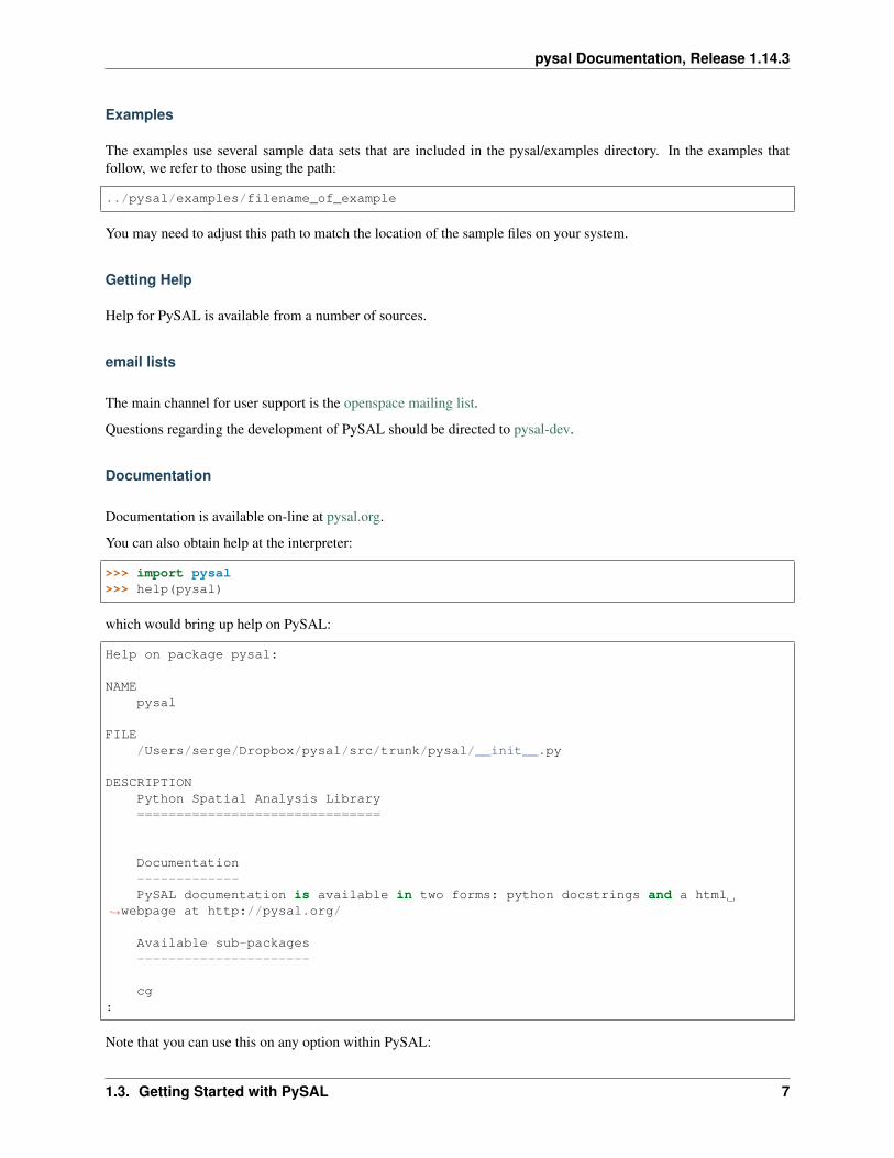
>>> import pysal>>> help(pysal)
which would bring up help on PySAL:
Help on package pysal:
NAMEpysal
FILE/Users/serge/Dropbox/pysal/src/trunk/pysal/__init__.py
DESCRIPTIONPython Spatial Analysis Library===============================
Documentation-------------PySAL documentation is available in two forms: python docstrings and a html
→˓webpage at http://pysal.org/
Available sub-packages----------------------
cg:
Note that you can use this on any option within PySAL:
1.3. Getting Started with PySAL 7
pysal Documentation, Release 1.14.3
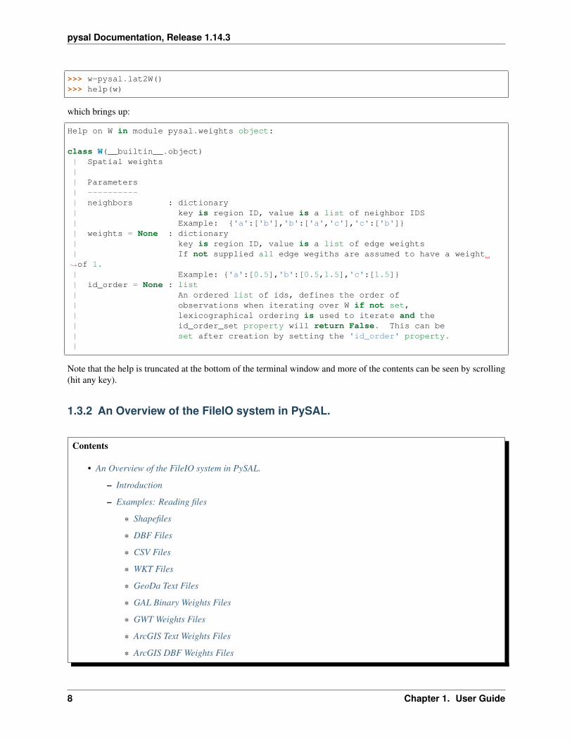
>>> w=pysal.lat2W()>>> help(w)
which brings up:
Help on W in module pysal.weights object:
class W(__builtin__.object)| Spatial weights|| Parameters| ----------| neighbors : dictionary| key is region ID, value is a list of neighbor IDS| Example: {'a':['b'],'b':['a','c'],'c':['b']}| weights = None : dictionary| key is region ID, value is a list of edge weights| If not supplied all edge wegiths are assumed to have a weight→˓of 1.| Example: {'a':[0.5],'b':[0.5,1.5],'c':[1.5]}| id_order = None : list| An ordered list of ids, defines the order of| observations when iterating over W if not set,| lexicographical ordering is used to iterate and the| id_order_set property will return False. This can be| set after creation by setting the 'id_order' property.|
Note that the help is truncated at the bottom of the terminal window and more of the contents can be seen by scrolling(hit any key).
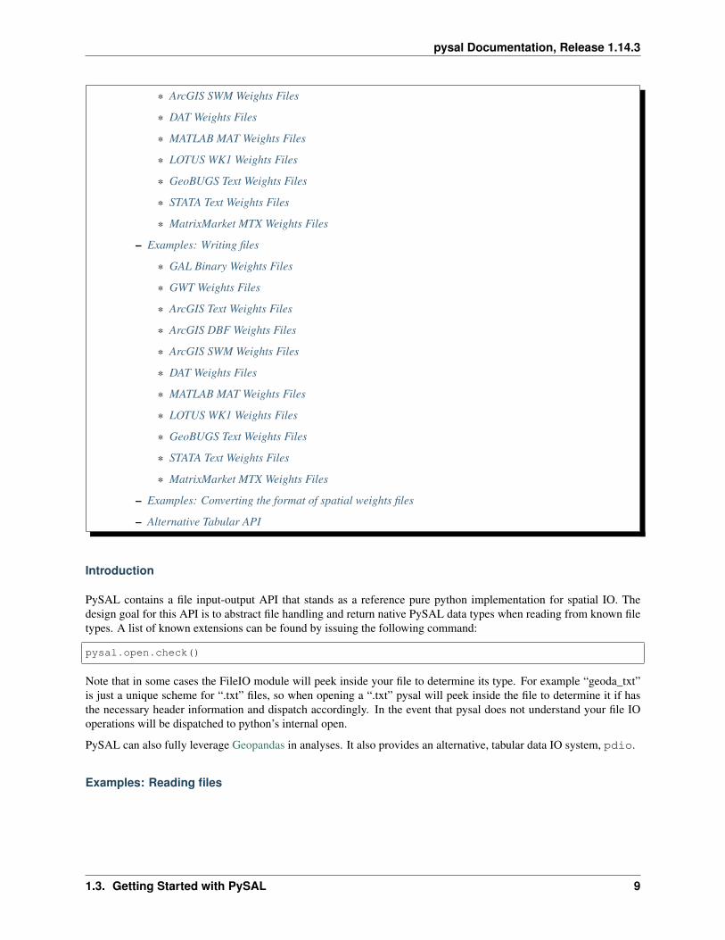
1.3.2 An Overview of the FileIO system in PySAL.
Contents
• An Overview of the FileIO system in PySAL.
– Introduction
– Examples: Reading files
* Shapefiles
* DBF Files
* CSV Files
* WKT Files
* GeoDa Text Files
* GAL Binary Weights Files
* GWT Weights Files
* ArcGIS Text Weights Files
* ArcGIS DBF Weights Files
8 Chapter 1. User Guide
pysal Documentation, Release 1.14.3
* ArcGIS SWM Weights Files
* DAT Weights Files
* MATLAB MAT Weights Files
* LOTUS WK1 Weights Files
* GeoBUGS Text Weights Files
* STATA Text Weights Files
* MatrixMarket MTX Weights Files
– Examples: Writing files
* GAL Binary Weights Files
* GWT Weights Files
* ArcGIS Text Weights Files
* ArcGIS DBF Weights Files
* ArcGIS SWM Weights Files
* DAT Weights Files
* MATLAB MAT Weights Files
* LOTUS WK1 Weights Files
* GeoBUGS Text Weights Files
* STATA Text Weights Files
* MatrixMarket MTX Weights Files
– Examples: Converting the format of spatial weights files
– Alternative Tabular API
Introduction
PySAL contains a file input-output API that stands as a reference pure python implementation for spatial IO. Thedesign goal for this API is to abstract file handling and return native PySAL data types when reading from known filetypes. A list of known extensions can be found by issuing the following command:
pysal.open.check()
Note that in some cases the FileIO module will peek inside your file to determine its type. For example “geoda_txt”is just a unique scheme for “.txt” files, so when opening a “.txt” pysal will peek inside the file to determine it if hasthe necessary header information and dispatch accordingly. In the event that pysal does not understand your file IOoperations will be dispatched to python’s internal open.
PySAL can also fully leverage Geopandas in analyses. It also provides an alternative, tabular data IO system, pdio.
Examples: Reading files
1.3. Getting Started with PySAL 9
pysal Documentation, Release 1.14.3
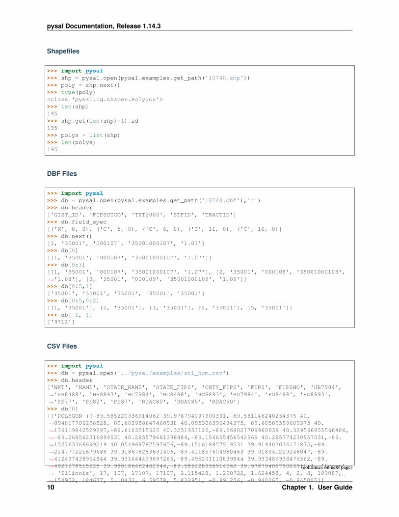
Shapefiles
>>> import pysal>>> shp = pysal.open(pysal.examples.get_path('10740.shp'))>>> poly = shp.next()>>> type(poly)<class 'pysal.cg.shapes.Polygon'>>>> len(shp)195>>> shp.get(len(shp)-1).id195>>> polys = list(shp)>>> len(polys)195
DBF Files
>>> import pysal>>> db = pysal.open(pysal.examples.get_path('10740.dbf'),'r')>>> db.header['GIST_ID', 'FIPSSTCO', 'TRT2000', 'STFID', 'TRACTID']>>> db.field_spec[('N', 8, 0), ('C', 5, 0), ('C', 6, 0), ('C', 11, 0), ('C', 10, 0)]>>> db.next()[1, '35001', '000107', '35001000107', '1.07']>>> db[0][[1, '35001', '000107', '35001000107', '1.07']]>>> db[0:3][[1, '35001', '000107', '35001000107', '1.07'], [2, '35001', '000108', '35001000108',→˓'1.08'], [3, '35001', '000109', '35001000109', '1.09']]>>> db[0:5,1]['35001', '35001', '35001', '35001', '35001']>>> db[0:5,0:2][[1, '35001'], [2, '35001'], [3, '35001'], [4, '35001'], [5, '35001']]>>> db[-1,-1]['9712']
CSV Files
>>> import pysal>>> db = pysal.open('../pysal/examples/stl_hom.csv')>>> db.header['WKT', 'NAME', 'STATE_NAME', 'STATE_FIPS', 'CNTY_FIPS', 'FIPS', 'FIPSNO', 'HR7984',→˓'HR8488', 'HR8893', 'HC7984', 'HC8488', 'HC8893', 'PO7984', 'PO8488', 'PO8893',→˓'PE77', 'PE82', 'PE87', 'RDAC80', 'RDAC85', 'RDAC90']>>> db[0][['POLYGON ((-89.585220336914062 39.978794097900391,-89.581146240234375 40.→˓094867706298828,-89.603988647460938 40.095306396484375,-89.60589599609375 40.→˓136119842529297,-89.6103515625 40.3251953125,-89.269027709960938 40.329566955566406,→˓-89.268562316894531 40.285579681396484,-89.154655456542969 40.285774230957031,-89.→˓152763366699219 40.054969787597656,-89.151618957519531 39.919403076171875,-89.→˓224777221679688 39.918678283691406,-89.411857604980469 39.918041229248047,-89.→˓412437438964844 39.931644439697266,-89.495201110839844 39.933486938476562,-89.→˓4927978515625 39.980186462402344,-89.585220336914062 39.978794097900391))', 'Logan',→˓ 'Illinois', 17, 107, 17107, 17107, 2.115428, 1.290722, 1.624458, 4, 2, 3, 189087,→˓154952, 184677, 5.10432, 6.59578, 5.832951, -0.991256, -0.940265, -0.845005]]
(continues on next page)
10 Chapter 1. User Guide
pysal Documentation, Release 1.14.3
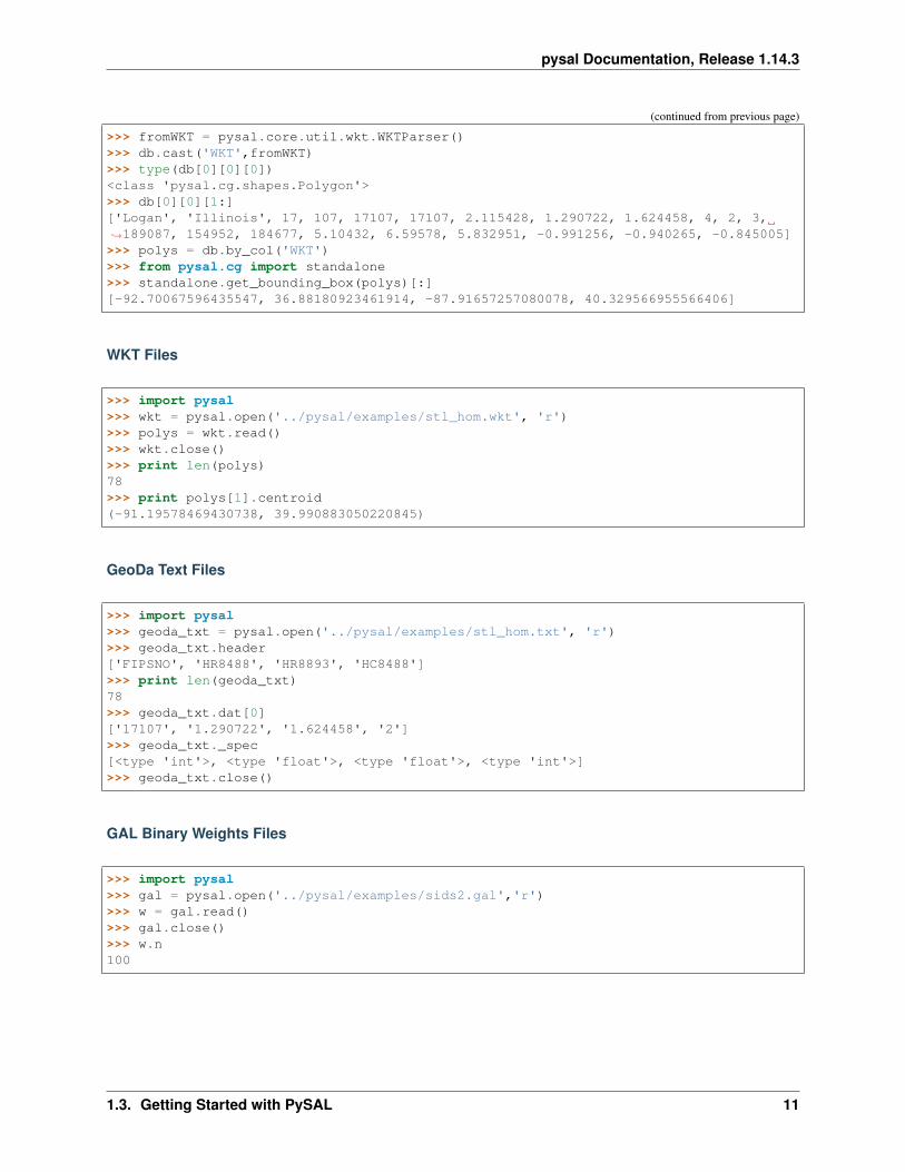
(continued from previous page)
>>> fromWKT = pysal.core.util.wkt.WKTParser()>>> db.cast('WKT',fromWKT)>>> type(db[0][0][0])<class 'pysal.cg.shapes.Polygon'>>>> db[0][0][1:]['Logan', 'Illinois', 17, 107, 17107, 17107, 2.115428, 1.290722, 1.624458, 4, 2, 3,→˓189087, 154952, 184677, 5.10432, 6.59578, 5.832951, -0.991256, -0.940265, -0.845005]>>> polys = db.by_col('WKT')>>> from pysal.cg import standalone>>> standalone.get_bounding_box(polys)[:][-92.70067596435547, 36.88180923461914, -87.91657257080078, 40.329566955566406]
WKT Files
>>> import pysal>>> wkt = pysal.open('../pysal/examples/stl_hom.wkt', 'r')>>> polys = wkt.read()>>> wkt.close()>>> print len(polys)78>>> print polys[1].centroid(-91.19578469430738, 39.990883050220845)
GeoDa Text Files
>>> import pysal>>> geoda_txt = pysal.open('../pysal/examples/stl_hom.txt', 'r')>>> geoda_txt.header['FIPSNO', 'HR8488', 'HR8893', 'HC8488']>>> print len(geoda_txt)78>>> geoda_txt.dat[0]['17107', '1.290722', '1.624458', '2']>>> geoda_txt._spec[<type 'int'>, <type 'float'>, <type 'float'>, <type 'int'>]>>> geoda_txt.close()
GAL Binary Weights Files
>>> import pysal>>> gal = pysal.open('../pysal/examples/sids2.gal','r')>>> w = gal.read()>>> gal.close()>>> w.n100
1.3. Getting Started with PySAL 11

pysal Documentation, Release 1.14.3
GWT Weights Files
>>> import pysal>>> gwt = pysal.open('../pysal/examples/juvenile.gwt', 'r')>>> w = gwt.read()>>> gwt.close()>>> w.n168
ArcGIS Text Weights Files
>>> import pysal>>> arcgis_txt = pysal.open('../pysal/examples/arcgis_txt.txt','r','arcgis_text')>>> w = arcgis_txt.read()>>> arcgis_txt.close()>>> w.n3
ArcGIS DBF Weights Files
>>> import pysal>>> arcgis_dbf = pysal.open('../pysal/examples/arcgis_ohio.dbf','r','arcgis_dbf')>>> w = arcgis_dbf.read()>>> arcgis_dbf.close()>>> w.n88
ArcGIS SWM Weights Files
>>> import pysal>>> arcgis_swm = pysal.open('../pysal/examples/ohio.swm','r')>>> w = arcgis_swm.read()>>> arcgis_swm.close()>>> w.n88
DAT Weights Files
>>> import pysal>>> dat = pysal.open('../pysal/examples/wmat.dat','r')>>> w = dat.read()>>> dat.close()>>> w.n49
12 Chapter 1. User Guide
pysal Documentation, Release 1.14.3
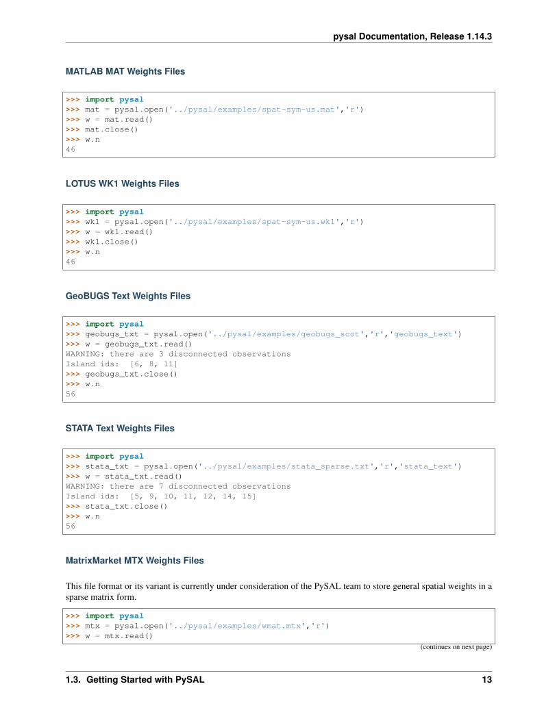
MATLAB MAT Weights Files
>>> import pysal>>> mat = pysal.open('../pysal/examples/spat-sym-us.mat','r')>>> w = mat.read()>>> mat.close()>>> w.n46
LOTUS WK1 Weights Files
>>> import pysal>>> wk1 = pysal.open('../pysal/examples/spat-sym-us.wk1','r')>>> w = wk1.read()>>> wk1.close()>>> w.n46
GeoBUGS Text Weights Files
>>> import pysal>>> geobugs_txt = pysal.open('../pysal/examples/geobugs_scot','r','geobugs_text')>>> w = geobugs_txt.read()WARNING: there are 3 disconnected observationsIsland ids: [6, 8, 11]>>> geobugs_txt.close()>>> w.n56
STATA Text Weights Files
>>> import pysal>>> stata_txt = pysal.open('../pysal/examples/stata_sparse.txt','r','stata_text')>>> w = stata_txt.read()WARNING: there are 7 disconnected observationsIsland ids: [5, 9, 10, 11, 12, 14, 15]>>> stata_txt.close()>>> w.n56
MatrixMarket MTX Weights Files
This file format or its variant is currently under consideration of the PySAL team to store general spatial weights in asparse matrix form.
>>> import pysal>>> mtx = pysal.open('../pysal/examples/wmat.mtx','r')>>> w = mtx.read()
(continues on next page)
1.3. Getting Started with PySAL 13
pysal Documentation, Release 1.14.3
(continued from previous page)
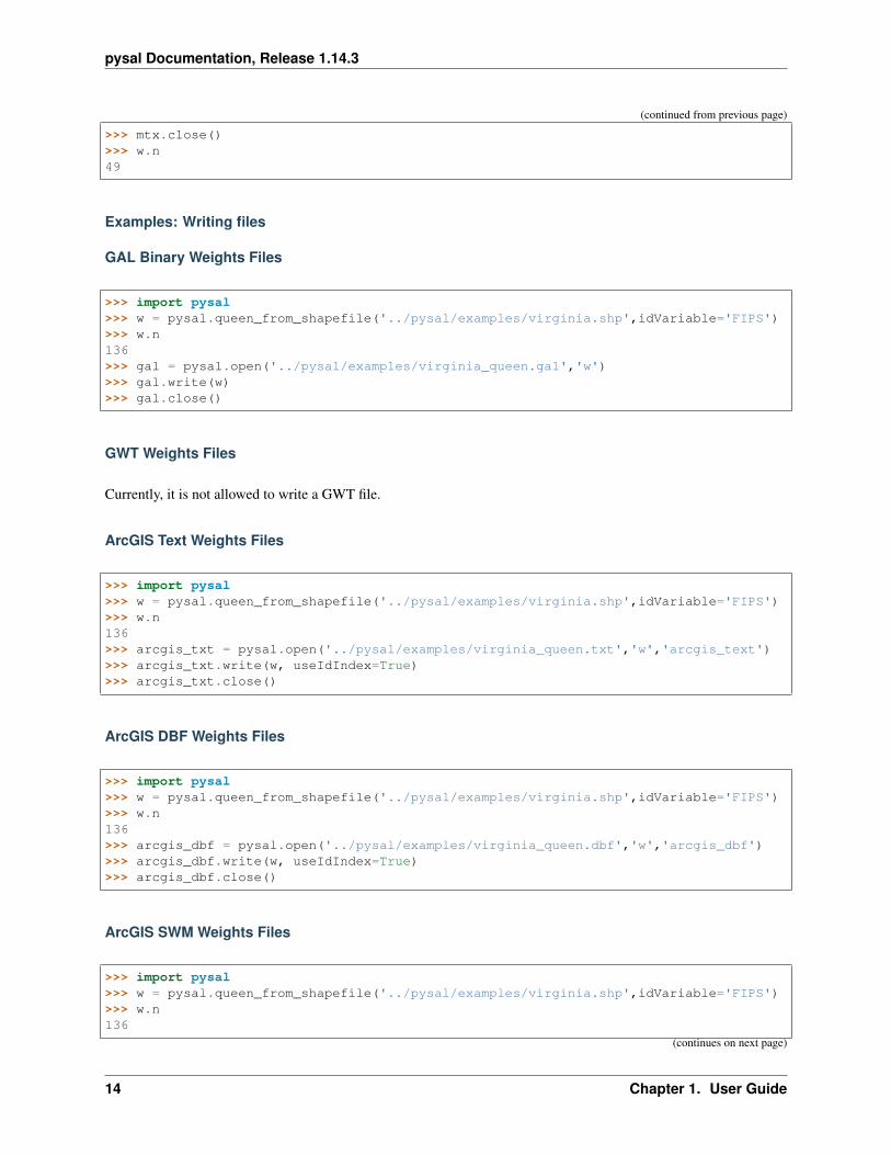
>>> mtx.close()>>> w.n49
Examples: Writing files
GAL Binary Weights Files
>>> import pysal>>> w = pysal.queen_from_shapefile('../pysal/examples/virginia.shp',idVariable='FIPS')>>> w.n136>>> gal = pysal.open('../pysal/examples/virginia_queen.gal','w')>>> gal.write(w)>>> gal.close()
GWT Weights Files
Currently, it is not allowed to write a GWT file.
ArcGIS Text Weights Files
>>> import pysal>>> w = pysal.queen_from_shapefile('../pysal/examples/virginia.shp',idVariable='FIPS')>>> w.n136>>> arcgis_txt = pysal.open('../pysal/examples/virginia_queen.txt','w','arcgis_text')>>> arcgis_txt.write(w, useIdIndex=True)>>> arcgis_txt.close()
ArcGIS DBF Weights Files
>>> import pysal>>> w = pysal.queen_from_shapefile('../pysal/examples/virginia.shp',idVariable='FIPS')>>> w.n136>>> arcgis_dbf = pysal.open('../pysal/examples/virginia_queen.dbf','w','arcgis_dbf')>>> arcgis_dbf.write(w, useIdIndex=True)>>> arcgis_dbf.close()
ArcGIS SWM Weights Files
>>> import pysal>>> w = pysal.queen_from_shapefile('../pysal/examples/virginia.shp',idVariable='FIPS')>>> w.n136
(continues on next page)
14 Chapter 1. User Guide
pysal Documentation, Release 1.14.3
(continued from previous page)
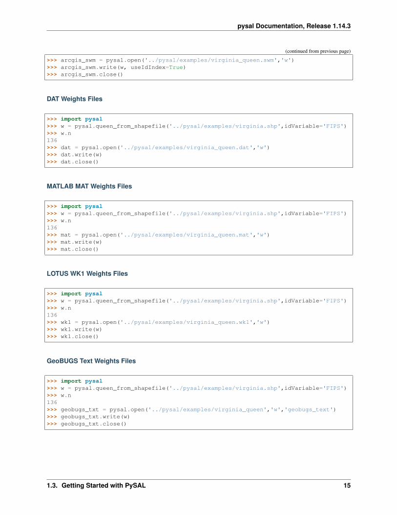
>>> arcgis_swm = pysal.open('../pysal/examples/virginia_queen.swm','w')>>> arcgis_swm.write(w, useIdIndex=True)>>> arcgis_swm.close()
DAT Weights Files
>>> import pysal>>> w = pysal.queen_from_shapefile('../pysal/examples/virginia.shp',idVariable='FIPS')>>> w.n136>>> dat = pysal.open('../pysal/examples/virginia_queen.dat','w')>>> dat.write(w)>>> dat.close()
MATLAB MAT Weights Files
>>> import pysal>>> w = pysal.queen_from_shapefile('../pysal/examples/virginia.shp',idVariable='FIPS')>>> w.n136>>> mat = pysal.open('../pysal/examples/virginia_queen.mat','w')>>> mat.write(w)>>> mat.close()
LOTUS WK1 Weights Files
>>> import pysal>>> w = pysal.queen_from_shapefile('../pysal/examples/virginia.shp',idVariable='FIPS')>>> w.n136>>> wk1 = pysal.open('../pysal/examples/virginia_queen.wk1','w')>>> wk1.write(w)>>> wk1.close()
GeoBUGS Text Weights Files
>>> import pysal>>> w = pysal.queen_from_shapefile('../pysal/examples/virginia.shp',idVariable='FIPS')>>> w.n136>>> geobugs_txt = pysal.open('../pysal/examples/virginia_queen','w','geobugs_text')>>> geobugs_txt.write(w)>>> geobugs_txt.close()
1.3. Getting Started with PySAL 15
pysal Documentation, Release 1.14.3
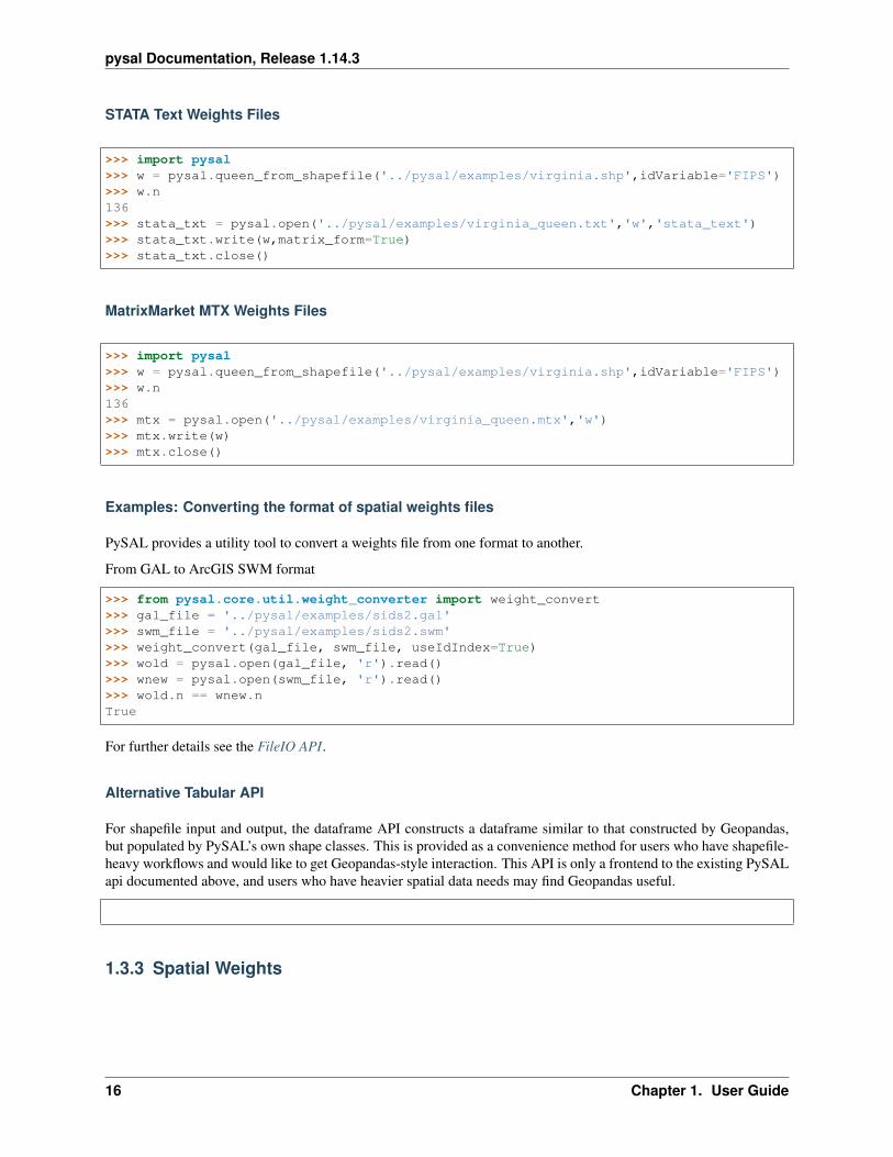
STATA Text Weights Files
>>> import pysal>>> w = pysal.queen_from_shapefile('../pysal/examples/virginia.shp',idVariable='FIPS')>>> w.n136>>> stata_txt = pysal.open('../pysal/examples/virginia_queen.txt','w','stata_text')>>> stata_txt.write(w,matrix_form=True)>>> stata_txt.close()
MatrixMarket MTX Weights Files
>>> import pysal>>> w = pysal.queen_from_shapefile('../pysal/examples/virginia.shp',idVariable='FIPS')>>> w.n136>>> mtx = pysal.open('../pysal/examples/virginia_queen.mtx','w')>>> mtx.write(w)>>> mtx.close()
Examples: Converting the format of spatial weights files
PySAL provides a utility tool to convert a weights file from one format to another.
From GAL to ArcGIS SWM format
>>> from pysal.core.util.weight_converter import weight_convert>>> gal_file = '../pysal/examples/sids2.gal'>>> swm_file = '../pysal/examples/sids2.swm'>>> weight_convert(gal_file, swm_file, useIdIndex=True)>>> wold = pysal.open(gal_file, 'r').read()>>> wnew = pysal.open(swm_file, 'r').read()>>> wold.n == wnew.nTrue
For further details see the FileIO API.
Alternative Tabular API
For shapefile input and output, the dataframe API constructs a dataframe similar to that constructed by Geopandas,but populated by PySAL’s own shape classes. This is provided as a convenience method for users who have shapefile-heavy workflows and would like to get Geopandas-style interaction. This API is only a frontend to the existing PySALapi documented above, and users who have heavier spatial data needs may find Geopandas useful.
1.3.3 Spatial Weights
16 Chapter 1. User Guide

pysal Documentation, Release 1.14.3
Contents
• Spatial Weights
– Introduction
– PySAL Spatial Weight Types
* Contiguity Based Weights
* Distance Based Weights
* k-nearest neighbor weights
* Distance band weights
* Kernel Weights
– Weights from other python objects
– A Closer look at W
* Attributes of W
* Weight Transformations
– W related functions
* Generating a full array
* Shimbel Matrices
* Higher Order Contiguity Weights
* Spatial Lag
* Non-Zero Diagonal
– WSets
* Union
* Intersection
* Difference
* Symmetric Difference
* Subset
– WSP
– Further Information
Introduction
Spatial weights are central components of many areas of spatial analysis. In general terms, for a spatial data setcomposed of n locations (points, areal units, network edges, etc.), the spatial weights matrix expresses the potentialfor interaction between observations at each pair i,j of locations. There is a rich variety of ways to specify the structureof these weights, and PySAL supports the creation, manipulation and analysis of spatial weights matrices across threedifferent general types:
• Contiguity Based Weights
• Distance Based Weights
1.3. Getting Started with PySAL 17

pysal Documentation, Release 1.14.3
• Kernel Weights
These different types of weights are implemented as instances or subclasses of the PySAL weights class W.
In what follows, we provide a high level overview of spatial weights in PySAL, starting with the three different typesof weights, followed by a closer look at the properties of the W class and some related functions.1
PySAL Spatial Weight Types
PySAL weights are handled in objects of the pysal.weights.W. The conceptual idea of spatial weights is that ofa nxn matrix in which the diagonal elements (𝑤𝑖𝑖) are set to zero by definition and the rest of the cells (𝑤𝑖𝑗) capturethe potential of interaction. However, these matrices tend to be fairly sparse (i.e. many cells contain zeros) and hencea full nxn array would not be an efficient representation. PySAL employs a different way of storing that is structuredin two main dictionaries2 : neighbors which, for each observation (key) contains a list of the other ones (value) withpotential for interaction (𝑤𝑖𝑗 ̸= 0); and weights, which contains the weight values for each of those observations (inthe same order). This way, large datasets can be stored when keeping the full matrix would not be possible because ofmemory constraints. In addition to the sparse representation via the weights and neighbors dictionaries, a PySAL Wobject also has an attribute called sparse, which is a scipy.sparse CSR representation of the spatial weights. (See WSPfor an alternative PySAL weights object.)
Contiguity Based Weights
To illustrate the general weights object, we start with a simple contiguity matrix constructed for a 5 by 5 lattice(composed of 25 spatial units):
>>> import pysal>>> w = pysal.lat2W(5, 5)
The w object has a number of attributes:
>>> w.n25>>> w.pct_nonzero12.8>>> w.weights[0][1.0, 1.0]>>> w.neighbors[0][5, 1]>>> w.neighbors[5][0, 10, 6]>>> w.histogram[(2, 4), (3, 12), (4, 9)]
n is the number of spatial units, so conceptually we could be thinking that the weights are stored in a 25x25 matrix.The second attribute (pct_nonzero) shows the sparseness of the matrix. The key attributes used to store contiguityrelations in W are the neighbors and weights attributes. In the example above we see that the observation with id 0(Python is zero-offset) has two neighbors with ids [5, 1] each of which have equal weights of 1.0.
The histogram attribute is a set of tuples indicating the cardinality of the neighbor relations. In this case we have aregular lattice, so there are 4 units that have 2 neighbors (corner cells), 12 units with 3 neighbors (edge cells), and 9units with 4 neighbors (internal cells).
1 Although this tutorial provides an introduction to the functionality of the PySAL weights class, it is not exhaustive. Complete documentationfor the class and associated functions can be found by accessing the help from within a Python interpreter.
2 The dictionaries for the weights and value attributes in W are read-only.
18 Chapter 1. User Guide

pysal Documentation, Release 1.14.3
In the above example, the default criterion for contiguity on the lattice was that of the rook which takes as neighborsany pair of cells that share an edge. Alternatively, we could have used the queen criterion to include the vertices of thelattice to define contiguities:
>>> wq = pysal.lat2W(rook = False)>>> wq.neighbors[0][5, 1, 6]
The bishop criterion, which designates pairs of cells as neighbors if they share only a vertex, is yet a third alternativefor contiguity weights. A bishop matrix can be computed as the Difference between the rook and queen cases.
The lat2W function is particularly useful in setting up simulation experiments requiring a regular grid. For empiricalresearch, a common use case is to have a shapefile, which is a nontopological vector data structure, and a need to carryout some form of spatial analysis that requires spatial weights. Since topology is not stored in the underlying file thereis a need to construct the spatial weights prior to carrying out the analysis.
In PySAL, weights are constructed by default from any contiguity graph representation. Most users will find the.from_shapefile methods most useful:
>>> w = pysal.weights.Rook.from_shapefile("../pysal/examples/columbus.shp")>>> w.n49>>> print "%.4f"%w.pct_nonzero0.0833>>> w.histogram[(2, 7), (3, 10), (4, 17), (5, 8), (6, 3), (7, 3), (8, 0), (9, 1)]
If queen, rather than rook, contiguity is required then the following would work:
>>> w = pysal.weights.Queen.from_shapefile("../pysal/examples/columbus.shp")>>> print "%.4f"%w.pct_nonzero0.0983>>> w.histogram[(2, 5), (3, 9), (4, 12), (5, 5), (6, 9), (7, 3), (8, 4), (9, 1), (10, 1)]
In addition to these methods, contiguity weights can be built from dataframes with a geometry column. This includesdataframes built from geopandas or from the PySAL pandas IO extension, pdio. For instance:
>>> import geopandas as gpd>>> test = gpd.read_file(pysal.examples.get_path('south.shp'))>>> W = pysal.weights.Queen.from_dataframe(test)>>> Wrook = pysal.weights.Rook.from_dataframe(test, idVariable='CNTY_FIPS')>>> pdiodf = pysal.pdio.read_files(pysal.examples.get_path('south.shp'))>>> W = pysal.weights.Rook.from_dataframe(pdiodf)
Or, weights can be constructed directly from an interable of shapely objects:
>>> import geopandas as gpd>>> shapelist = gpd.read_file(pysal.examples.get_path('columbus.shp')).geometry.→˓tolist()>>> W = pysal.weights.Queen.from_iterable(shapelist)
The .from_file method on contigutiy weights simply passes down to the parent class’s .from_file method,so the returned object is of instance W, not Queen or Rook. This occurs because the weights cannot be verified ascontiguity weights without the original shapes.
1.3. Getting Started with PySAL 19
pysal Documentation, Release 1.14.3
>>> W = pysal.weights.Rook.from_file(pysal.examples.get_path('columbus.gal')>>> type(W)pysal.weights.weights.W
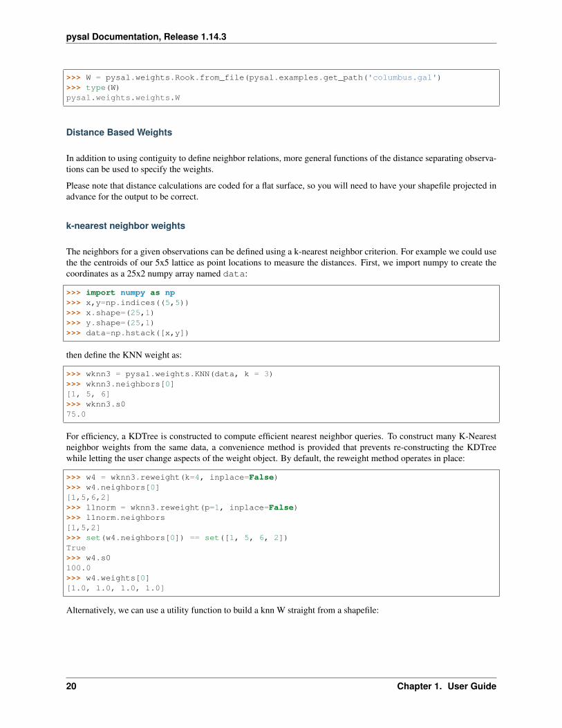
Distance Based Weights
In addition to using contiguity to define neighbor relations, more general functions of the distance separating observa-tions can be used to specify the weights.
Please note that distance calculations are coded for a flat surface, so you will need to have your shapefile projected inadvance for the output to be correct.
k-nearest neighbor weights
The neighbors for a given observations can be defined using a k-nearest neighbor criterion. For example we could usethe the centroids of our 5x5 lattice as point locations to measure the distances. First, we import numpy to create thecoordinates as a 25x2 numpy array named data:
>>> import numpy as np>>> x,y=np.indices((5,5))>>> x.shape=(25,1)>>> y.shape=(25,1)>>> data=np.hstack([x,y])
then define the KNN weight as:
>>> wknn3 = pysal.weights.KNN(data, k = 3)>>> wknn3.neighbors[0][1, 5, 6]>>> wknn3.s075.0
For efficiency, a KDTree is constructed to compute efficient nearest neighbor queries. To construct many K-Nearestneighbor weights from the same data, a convenience method is provided that prevents re-constructing the KDTreewhile letting the user change aspects of the weight object. By default, the reweight method operates in place:
>>> w4 = wknn3.reweight(k=4, inplace=False)>>> w4.neighbors[0][1,5,6,2]>>> l1norm = wknn3.reweight(p=1, inplace=False)>>> l1norm.neighbors[1,5,2]>>> set(w4.neighbors[0]) == set([1, 5, 6, 2])True>>> w4.s0100.0>>> w4.weights[0][1.0, 1.0, 1.0, 1.0]
Alternatively, we can use a utility function to build a knn W straight from a shapefile:
20 Chapter 1. User Guide

pysal Documentation, Release 1.14.3
>>> wknn5 = pysal.weights.KNN.from_shapefile(pysal.examples.get_path('columbus.shp'),→˓k=5)>>> wknn5.neighbors[0][2, 1, 3, 7, 4]
Or from a dataframe:
>>> import geopandas as gpd>>> df = gpd.read_file(ps.examples.get_path('baltim.shp'))>>> k5 = pysal.weights.KNN.from_dataframe(df, k=5)
Distance band weights
Knn weights ensure that all observations have the same number of neighbors.3 An alternative distance based set ofweights relies on distance bands or thresholds to define the neighbor set for each spatial unit as those other units fallingwithin a threshold distance of the focal unit:
>>> wthresh = pysal.weights.DistanceBand.from_array(data, 2)>>> set(wthresh.neighbors[0]) == set([1, 2, 5, 6, 10])True>>> set(wthresh.neighbors[1]) == set( [0, 2, 5, 6, 7, 11, 3])True>>> wthresh.weights[0][1, 1, 1, 1, 1]>>> wthresh.weights[1][1, 1, 1, 1, 1, 1, 1]>>>
As can be seen in the above example, the number of neighbors is likely to vary across observations with distance bandweights in contrast to what holds for knn weights.
In addition to constructing these from the helper function, Distance Band weights. For example, a threshold binary Wcan be constructed from a dataframe:
>>> import geopandas as gpd>>> df = gpd.read_file(ps.examples.get_path('baltim.shp'))>>> ps.weights.DistanceBand.from_dataframe(df, threshold=6, binary=True)
Distance band weights can be generated for shapefiles as well as arrays of points.4 First, the minimum nearest neighbordistance should be determined so that each unit is assured of at least one neighbor:
>>> thresh = pysal.min_threshold_dist_from_shapefile("../pysal/examples/columbus.shp")>>> thresh0.61886415807685413
with this threshold in hand, the distance band weights are obtained as:
>>> wt = pysal.weights.DistanceBand.from_shapefile("../pysal/examples/columbus.shp",→˓threshold=thresh, binary=True)>>> wt.min_neighbors1>>> wt.histogram
(continues on next page)
3 Ties at the k-nn distance band are randomly broken to ensure each observation has exactly k neighbors.4 If the shapefile contains geographical coordinates these distance calculations will be misleading and the user should first project their coordi-
nates using a GIS.
1.3. Getting Started with PySAL 21
pysal Documentation, Release 1.14.3
(continued from previous page)
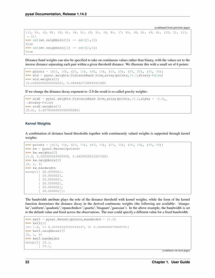
[(1, 4), (2, 8), (3, 6), (4, 2), (5, 5), (6, 8), (7, 6), (8, 2), (9, 6), (10, 1), (11,→˓ 1)]>>> set(wt.neighbors[0]) == set([1,2])True>>> set(wt.neighbors[1]) == set([3,0])True
Distance band weights can also be specified to take on continuous values rather than binary, with the values set to theinverse distance separating each pair within a given threshold distance. We illustrate this with a small set of 6 points:
>>> points = [(10, 10), (20, 10), (40, 10), (15, 20), (30, 20), (30, 30)]>>> wid = pysal.weights.DistanceBand.from_array(points,14.2,binary=False)>>> wid.weights[0][0.10000000000000001, 0.089442719099991588]
If we change the distance decay exponent to -2.0 the result is so called gravity weights:
>>> wid2 = pysal.weights.DistanceBand.from_array(points,14.2,alpha = -2.0,→˓binary=False)>>> wid2.weights[0][0.01, 0.0079999999999999984]
Kernel Weights
A combination of distance based thresholds together with continuously valued weights is supported through kernelweights:
>>> points = [(10, 10), (20, 10), (40, 10), (15, 20), (30, 20), (30, 30)]>>> kw = pysal.Kernel(points)>>> kw.weights[0][1.0, 0.500000049999995, 0.4409830615267465]>>> kw.neighbors[0][0, 1, 3]>>> kw.bandwidtharray([[ 20.000002],
[ 20.000002],[ 20.000002],[ 20.000002],[ 20.000002],[ 20.000002]])
The bandwidth attribute plays the role of the distance threshold with kernel weights, while the form of the kernelfunction determines the distance decay in the derived continuous weights (the following are available: ‘triangu-lar’,’uniform’,’quadratic’,’epanechnikov’,’quartic’,’bisquare’,’gaussian’). In the above example, the bandwidth is setto the default value and fixed across the observations. The user could specify a different value for a fixed bandwidth:
>>> kw15 = pysal.Kernel(points,bandwidth = 15.0)>>> kw15[0]{0: 1.0, 1: 0.33333333333333337, 3: 0.2546440075000701}>>> kw15.neighbors[0][0, 1, 3]>>> kw15.bandwidtharray([[ 15.],
[ 15.],
(continues on next page)
22 Chapter 1. User Guide

pysal Documentation, Release 1.14.3
(continued from previous page)
[ 15.],[ 15.],[ 15.],[ 15.]])
which results in fewer neighbors for the first unit. Adaptive bandwidths (i.e., different bandwidths for each unit) canalso be user specified:
>>> bw = [25.0,15.0,25.0,16.0,14.5,25.0]>>> kwa = pysal.Kernel(points,bandwidth = bw)>>> kwa.weights[0][1.0, 0.6, 0.552786404500042, 0.10557280900008403]>>> kwa.neighbors[0][0, 1, 3, 4]>>> kwa.bandwidtharray([[ 25. ],
[ 15. ],[ 25. ],[ 16. ],[ 14.5],[ 25. ]])
Alternatively the adaptive bandwidths could be defined endogenously:
>>> kwea = pysal.Kernel(points,fixed = False)>>> kwea.weights[0][1.0, 0.10557289844279438, 9.99999900663795e-08]>>> kwea.neighbors[0][0, 1, 3]>>> kwea.bandwidtharray([[ 11.18034101],
[ 11.18034101],[ 20.000002 ],[ 11.18034101],[ 14.14213704],[ 18.02775818]])
Finally, the kernel function could be changed (with endogenous adaptive bandwidths):
>>> kweag = pysal.Kernel(points,fixed = False,function = 'gaussian')>>> kweag.weights[0][0.3989422804014327, 0.2674190291577696, 0.2419707487162134]>>> kweag.bandwidtharray([[ 11.18034101],
[ 11.18034101],[ 20.000002 ],[ 11.18034101],[ 14.14213704],[ 18.02775818]])
More details on kernel weights can be found in Kernel. All kernel methods also support construction from shapefileswith Kernel.from_shapefile and from dataframes with Kernel.from_dataframe.
1.3. Getting Started with PySAL 23

pysal Documentation, Release 1.14.3
Weights from other python objects
PySAL weights can also be constructed easily from many other objects. Most importantly, all weight types can beconstructed directly from geopandas geodataframes using the .from_dataframe method. For distance andkernel weights, underlying features should typically be points. But, if polygons are supplied, the centroids of thepolygons will be used by default:
>>> import geopandas as gpd>>> df = gpd.read_file(pysal.examples.get_path('columbus.shp'))>>> kw = pysal.weights.Kernel.from_dataframe(df)>>> dbb = pysal.weights.DistanceBand.from_dataframe(df, threshold=.9, binary=False)>>> dbc = pysal.weights.DistanceBand.from_dataframe(df, threshold=.9, binary=True)>>> q = pysal.weights.Queen.from_dataframe(df)>>> r = pysal.weights.Rook.from_dataframe(df)
This also applies to dynamic views of the dataframe:
>>> q2 = pysal.weights.Queen.from_dataframe(df.query('DISCBD < 2'))
Weights can also be constructed from NetworkX objects. This is easiest to construct using a sparse weight, but thatcan be converted to a full dense PySAL weight easily:
>>> import networkx as nx>>> G = nx.random_lobster(50,.2,.5)>>> sparse_lobster = ps.weights.WSP(nx.adj_matrix(G))>>> dense_lobster = sparse_lobster.to_W()
A Closer look at W
Although the three different types of spatial weights illustrated above cover a wide array of approaches towards spec-ifying spatial relations, they all share common attributes from the base W class in PySAL. Here we take a closer lookat some of the more useful properties of this class.
Attributes of W
W objects come with a whole bunch of useful attributes that may help you when dealing with spatial weights matrices.To see a list of all of them, same as with any other Python object, type:
>>> import pysal>>> help(pysal.W)
If you want to be more specific and learn, for example, about the attribute s0, then type:
>>> help(pysal.W.s0)Help on property:
float
𝑠0 =∑︁𝑖
∑︁𝑗
𝑤𝑖,𝑗
24 Chapter 1. User Guide
pysal Documentation, Release 1.14.3
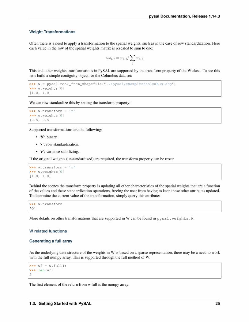
Weight Transformations
Often there is a need to apply a transformation to the spatial weights, such as in the case of row standardization. Hereeach value in the row of the spatial weights matrix is rescaled to sum to one:
𝑤𝑠𝑖,𝑗 = 𝑤𝑖,𝑗/∑︁𝑗
𝑤𝑖,𝑗
This and other weights transformations in PySAL are supported by the transform property of the W class. To see thislet’s build a simple contiguity object for the Columbus data set:
>>> w = pysal.rook_from_shapefile("../pysal/examples/columbus.shp")>>> w.weights[0][1.0, 1.0]
We can row standardize this by setting the transform property:
>>> w.transform = 'r'>>> w.weights[0][0.5, 0.5]
Supported transformations are the following:
• ‘b’: binary.
• ‘r’: row standardization.
• ‘v’: variance stabilizing.
If the original weights (unstandardized) are required, the transform property can be reset:
>>> w.transform = 'o'>>> w.weights[0][1.0, 1.0]
Behind the scenes the transform property is updating all other characteristics of the spatial weights that are a functionof the values and these standardization operations, freeing the user from having to keep these other attributes updated.To determine the current value of the transformation, simply query this attribute:
>>> w.transform'O'
More details on other transformations that are supported in W can be found in pysal.weights.W.
W related functions
Generating a full array
As the underlying data structure of the weights in W is based on a sparse representation, there may be a need to workwith the full numpy array. This is supported through the full method of W:
>>> wf = w.full()>>> len(wf)2
The first element of the return from w.full is the numpy array:
1.3. Getting Started with PySAL 25
pysal Documentation, Release 1.14.3
>>> wf[0].shape(49, 49)
while the second element contains the ids for the row (column) ordering of the array:
>>> wf[1][0:5][0, 1, 2, 3, 4]
If only the array is required, a simple Python slice can be used:
>>> wf = w.full()[0]
Shimbel Matrices
The Shimbel matrix for a set of n objects contains the shortest path distance separating each pair of units. This haswide use in spatial analysis for solving different types of clustering and optimization problems. Using the functionshimbel with a W instance as an argument generates this information:
>>> w = pysal.lat2W(3,3)>>> ws = pysal.shimbel(w)>>> ws[0][-1, 1, 2, 1, 2, 3, 2, 3, 4]
Thus we see that observation 0 (the northwest cell of our 3x3 lattice) is a first order neighbor to observations 1 and 3,second order neighbor to observations 2, 4, and 6, a third order neighbor to 5, and 7, and a fourth order neighbor toobservation 8 (the extreme southeast cell in the lattice). The position of the -1 simply denotes the focal unit.
Higher Order Contiguity Weights
Closely related to the shortest path distances is the concept of a spatial weight based on a particular order of contiguity.For example, we could define the second order contiguity relations using:
>>> w2 = pysal.higher_order(w, 2)>>> w2.neighbors[0][4, 6, 2]
or a fourth order set of weights:
>>> w4 = pysal.higher_order(w, 4)WARNING: there are 5 disconnected observationsIsland ids: [1, 3, 4, 5, 7]>>> w4.neighbors[0][8]
In both cases a new instance of the W class is returned with the weights and neighbors defined using the particularorder of contiguity.
Spatial Lag
The final function related to spatial weights that we illustrate here is used to construct a new variable called the spatiallag. The spatial lag is a function of the attribute values observed at neighboring locations. For example, if we continuewith our regular 3x3 lattice and create an attribute variable y:
26 Chapter 1. User Guide

pysal Documentation, Release 1.14.3
>>> import numpy as np>>> y = np.arange(w.n)>>> yarray([0, 1, 2, 3, 4, 5, 6, 7, 8])
then the spatial lag can be constructed with:
>>> yl = pysal.lag_spatial(w,y)>>> ylarray([ 4., 6., 6., 10., 16., 14., 10., 18., 12.])
Mathematically, the spatial lag is a weighted sum of neighboring attribute values
𝑦𝑙𝑖 =∑︁𝑗
𝑤𝑖,𝑗𝑦𝑗
In the example above, the weights were binary, based on the rook criterion. If we row standardize our W object firstand then recalculate the lag, it takes the form of a weighted average of the neighboring attribute values:
>>> w.transform = 'r'>>> ylr = pysal.lag_spatial(w,y)>>> ylrarray([ 2. , 2. , 3. , 3.33333333, 4. ,
4.66666667, 5. , 6. , 6. ])
One important consideration in calculating the spatial lag is that the ordering of the values in y aligns with the under-lying order in W. In cases where the source for your attribute data is different from the one to construct your weightsyou may need to reorder your y values accordingly. To check if this is the case you can find the order in W as follows:
>>> w.id_order[0, 1, 2, 3, 4, 5, 6, 7, 8]
In this case the lag_spatial function assumes that the first value in the y attribute corresponds to unit 0 in the lattice(northwest cell), while the last value in y would correspond to unit 8 (southeast cell). In other words, for the value ofthe spatial lag to be valid the number of elements in y must match w.n and the orderings must be aligned.
Fortunately, for the common use case where both the attribute and weights information come from a shapefile (and itsdbf), PySAL handles the alignment automatically:5
>>> w = pysal.rook_from_shapefile("../pysal/examples/columbus.shp")>>> f = pysal.open("../pysal/examples/columbus.dbf")>>> f.header['AREA', 'PERIMETER', 'COLUMBUS_', 'COLUMBUS_I', 'POLYID', 'NEIG', 'HOVAL', 'INC',→˓'CRIME', 'OPEN', 'PLUMB', 'DISCBD', 'X', 'Y', 'NSA', 'NSB', 'EW', 'CP', 'THOUS',→˓'NEIGNO']>>> y = np.array(f.by_col['INC'])>>> w.transform = 'r'>>> yarray([ 19.531 , 21.232 , 15.956 , 4.477 , 11.252 ,
16.028999, 8.438 , 11.337 , 17.586 , 13.598 ,7.467 , 10.048 , 9.549 , 9.963 , 9.873 ,7.625 , 9.798 , 13.185 , 11.618 , 31.07 ,10.655 , 11.709 , 21.155001, 14.236 , 8.461 ,8.085 , 10.822 , 7.856 , 8.681 , 13.906 ,16.940001, 18.941999, 9.918 , 14.948 , 12.814 ,
(continues on next page)
5 The ordering exploits the one-to-one relation between a record in the DBF file and the shape in the shapefile.
1.3. Getting Started with PySAL 27

pysal Documentation, Release 1.14.3
(continued from previous page)
18.739 , 17.017 , 11.107 , 18.476999, 29.833 ,22.207001, 25.872999, 13.38 , 16.961 , 14.135 ,18.323999, 18.950001, 11.813 , 18.796 ])
>>> yl = pysal.lag_spatial(w,y)>>> ylarray([ 18.594 , 13.32133333, 14.123 , 14.94425 ,
11.817857 , 14.419 , 10.283 , 8.3364 ,11.7576665 , 19.48466667, 10.0655 , 9.1882 ,9.483 , 10.07716667, 11.231 , 10.46185714,21.94100033, 10.8605 , 12.46133333, 15.39877778,14.36333333, 15.0838 , 19.93666633, 10.90833333,9.7 , 11.403 , 15.13825 , 10.448 ,11.81 , 12.64725 , 16.8435 , 26.0662505 ,15.6405 , 18.05175 , 15.3824 , 18.9123996 ,12.2418 , 12.76675 , 18.5314995 , 22.79225025,22.575 , 16.8435 , 14.2066 , 14.20075 ,15.2515 , 18.6079995 , 26.0200005 , 15.818 , 14.303 ])
>>> w.id_order[0, 1, 2, 3, 4, 5, 6, 7, 8, 9, 10, 11, 12, 13, 14, 15, 16, 17, 18, 19, 20, 21, 22, 23,→˓ 24, 25, 26, 27, 28, 29, 30, 31, 32, 33, 34, 35, 36, 37, 38, 39, 40, 41, 42, 43, 44,→˓ 45, 46, 47, 48]
Non-Zero Diagonal
The typical weights matrix has zeros along the main diagonal. This has the practical result of excluding the self fromany computation. However, this is not always the desired situation, and so PySAL offers a function that adds valuesto the main diagonal of a W object.
As an example, we can build a basic rook weights matrix, which has zeros on the diagonal, then insert ones along thediagonal:
>>> w = pysal.lat2W(5, 5, id_type='string')>>> w['id0']{'id5': 1.0, 'id1': 1.0}>>> w_const = pysal.weights.insert_diagonal(w)>>> w_const['id0']{'id5': 1.0, 'id0': 1.0, 'id1': 1.0}
The default is to add ones to the diagonal, but the function allows any values to be added.
WSets
PySAL offers set-like manipulation of spatial weights matrices. While a W is more complex than a set, the twoobjects have a number of commonalities allowing for traditional set operations to have similar functionality on a W.Conceptually, we treat each neighbor pair as an element of a set, and then return the appropriate pairs based on theoperation invoked (e.g. union, intersection, etc.). A key distinction between a set and a W is that a W must keep trackof the universe of possible pairs, even those that do not result in a neighbor relationship.
PySAL follows the naming conventions for Python sets, but adds optional flags allowing the user to control the shapeof the weights object returned. At this time, all the functions discussed in this section return a binary W no matter theweights objects passed in.
28 Chapter 1. User Guide
pysal Documentation, Release 1.14.3
Union
The union of two weights objects returns a binary weights object, W, that includes all neighbor pairs that exist in eitherweights object. This function can be used to simply join together two weights objects, say one for Arizona countiesand another for California counties. It can also be used to join two weights objects that overlap as in the examplebelow.
>>> w1 = pysal.lat2W(4,4)>>> w2 = pysal.lat2W(6,4)>>> w = pysal.w_union(w1, w2)>>> w1[0] == w[0]True>>> w1.neighbors[15][11, 14]>>> w2.neighbors[15][11, 14, 19]>>> w.neighbors[15][19, 11, 14]
Intersection
The intersection of two weights objects returns a binary weights object, W, that includes only those neighbor pairsthat exist in both weights objects. Unlike the union case, where all pairs in either matrix are returned, the intersectiononly returns a subset of the pairs. This leaves open the question of the shape of the weights matrix to return. Forexample, you have one weights matrix of census tracts for City A and second matrix of tracts for Utility Company B’sservice area, and want to find the W for the tracts that overlap. Depending on the research question, you may want thereturned W to have the same dimensions as City A’s weights matrix, the same as the utility company’s weights matrix,a new dimensionality based on all the census tracts in either matrix or with the dimensionality of just those tracts inthe overlapping area. All of these options are available via the w_shape parameter and the order that the matrices arepassed to the function. The following example uses the all case:
>>> w1 = pysal.lat2W(4,4)>>> w2 = pysal.lat2W(6,4)>>> w = pysal.w_intersection(w1, w2, 'all')WARNING: there are 8 disconnected observationsIsland ids: [16, 17, 18, 19, 20, 21, 22, 23]>>> w1[0] == w[0]True>>> w1.neighbors[15][11, 14]>>> w2.neighbors[15][11, 14, 19]>>> w.neighbors[15][11, 14]>>> w2.neighbors[16][12, 20, 17]>>> w.neighbors[16][]
Difference
The difference of two weights objects returns a binary weights object, W, that includes only neighbor pairs from thefirst object that are not in the second. Similar to the intersection function, the user must select the shape of the weights
1.3. Getting Started with PySAL 29
pysal Documentation, Release 1.14.3
object returned using the w_shape parameter. The user must also consider the constrained parameter which controlswhether the observations and the neighbor pairs are differenced or just the neighbor pairs are differenced. If you wereto apply the difference function to our city and utility company example from the intersection section above, you mustdecide whether or not pairs that exist along the border of the regions should be considered different or not. It boils downto whether the tracts should be differenced first and then the differenced pairs identified (constrained=True), or if thedifferenced pairs should be identified based on the sets of pairs in the original weights matrices (constrained=False).In the example below we difference weights matrices from regions with partial overlap.
>>> w1 = pysal.lat2W(6,4)>>> w2 = pysal.lat2W(4,4)>>> w1.neighbors[15][11, 14, 19]>>> w2.neighbors[15][11, 14]>>> w = pysal.w_difference(w1, w2, w_shape = 'w1', constrained = False)WARNING: there are 12 disconnected observationsIsland ids: [0, 1, 2, 3, 4, 5, 6, 7, 8, 9, 10, 11]>>> w.neighbors[15][19]>>> w.neighbors[19][15, 18, 23]>>> w = pysal.w_difference(w1, w2, w_shape = 'min', constrained = False)>>> 15 in w.neighborsFalse>>> w.neighbors[19][18, 23]>>> w = pysal.w_difference(w1, w2, w_shape = 'w1', constrained = True)WARNING: there are 16 disconnected observationsIsland ids: [0, 1, 2, 3, 4, 5, 6, 7, 8, 9, 10, 11, 12, 13, 14, 15]>>> w.neighbors[15][]>>> w.neighbors[19][18, 23]>>> w = pysal.w_difference(w1, w2, w_shape = 'min', constrained = True)>>> 15 in w.neighborsFalse>>> w.neighbors[19][18, 23]
The difference function can be used to construct a bishop contiguity weights matrix by differencing a queen and rookmatrix.
>>> wr = pysal.lat2W(5,5)>>> wq = pysal.lat2W(5,5,rook = False)>>> wb = pysal.w_difference(wq, wr,constrained = False)>>> wb.neighbors[0][6]
Symmetric Difference
Symmetric difference of two weights objects returns a binary weights object, W, that includes only neighbor pairsthat are not shared by either matrix. This function offers options similar to those in the difference function describedabove.
30 Chapter 1. User Guide

pysal Documentation, Release 1.14.3
>>> w1 = pysal.lat2W(6, 4)>>> w2 = pysal.lat2W(2, 4)>>> w_lower = pysal.w_difference(w1, w2, w_shape = 'min', constrained = True)>>> w_upper = pysal.lat2W(4, 4)>>> w = pysal.w_symmetric_difference(w_lower, w_upper, 'all', False)>>> w_lower.id_order[8, 9, 10, 11, 12, 13, 14, 15, 16, 17, 18, 19, 20, 21, 22, 23]>>> w_upper.id_order[0, 1, 2, 3, 4, 5, 6, 7, 8, 9, 10, 11, 12, 13, 14, 15]>>> w.id_order[0, 1, 2, 3, 4, 5, 6, 7, 8, 9, 10, 11, 12, 13, 14, 15, 16, 17, 18, 19, 20, 21, 22, 23]>>> w.neighbors[11][7]>>> w = pysal.w_symmetric_difference(w_lower, w_upper, 'min', False)WARNING: there are 8 disconnected observationsIsland ids: [0, 1, 2, 3, 4, 5, 6, 7]>>> 11 in w.neighborsFalse>>> w.id_order[0, 1, 2, 3, 4, 5, 6, 7, 16, 17, 18, 19, 20, 21, 22, 23]>>> w = pysal.w_symmetric_difference(w_lower, w_upper, 'all', True)WARNING: there are 16 disconnected observationsIsland ids: [0, 1, 2, 3, 4, 5, 6, 7, 8, 9, 10, 11, 12, 13, 14, 15]>>> w.neighbors[11][]>>> w = pysal.w_symmetric_difference(w_lower, w_upper, 'min', True)WARNING: there are 8 disconnected observationsIsland ids: [0, 1, 2, 3, 4, 5, 6, 7]>>> 11 in w.neighborsFalse
Subset
Subset of a weights object returns a binary weights object, W, that includes only those observations provided by theuser. It also can be used to add islands to a previously existing weights object.
>>> w1 = pysal.lat2W(6, 4)>>> w1.id_order[0, 1, 2, 3, 4, 5, 6, 7, 8, 9, 10, 11, 12, 13, 14, 15, 16, 17, 18, 19, 20, 21, 22, 23]>>> ids = range(16)>>> w = pysal.w_subset(w1, ids)>>> w.id_order[0, 1, 2, 3, 4, 5, 6, 7, 8, 9, 10, 11, 12, 13, 14, 15]>>> w1[0] == w[0]True>>> w1.neighbors[15][11, 14, 19]>>> w.neighbors[15][11, 14]
WSP
A thin PySAL weights object is available to users with extremely large weights matrices, on the order of 2 million ormore observations, or users interested in holding many large weights matrices in RAM simultaneously. The pysal.
1.3. Getting Started with PySAL 31
pysal Documentation, Release 1.14.3
weights.WSP is a thin weights object that does not include the neighbors and weights dictionaries, but does containthe scipy.sparse form of the weights. For many PySAL functions the W and WSP objects can be used interchangeably.
A WSP object can be constructed from a Matrix Market file (see MatrixMarket MTX Weights Files for more info onreading and writing mtx files in PySAL):
>>> mtx = pysal.open("../pysal/examples/wmat.mtx", 'r')>>> wsp = mtx.read(sparse=True)
or built directly from a scipy.sparse object:
>>> import scipy.sparse>>> rows = [0, 1, 1, 2, 2, 3]>>> cols = [1, 0, 2, 1, 3, 3]>>> weights = [1, 0.75, 0.25, 0.9, 0.1, 1]>>> sparse = scipy.sparse.csr_matrix((weights, (rows, cols)), shape=(4,4))>>> w = pysal.weights.WSP(sparse)
The WSP object has subset of the attributes of a W object; for example:
>>> w.n4>>> w.s04.0>>> w.trcWtW_WW6.3949999999999996
The following functionality is available to convert from a W to a WSP:
>>> w = pysal.weights.lat2W(5,5)>>> w.s080.0>>> wsp = pysal.weights.WSP(w.sparse)>>> wsp.s080.0
and from a WSP to W:
>>> sp = pysal.weights.lat2SW(5, 5)>>> wsp = pysal.weights.WSP(sp)>>> wsp.s080>>> w = pysal.weights.WSP2W(wsp)>>> w.s080
Further Information
For further details see the Weights API.
1.3.4 Spatial Autocorrelation
Contents
32 Chapter 1. User Guide
pysal Documentation, Release 1.14.3
• Spatial Autocorrelation
– Introduction
– Global Autocorrelation
* Gamma Index of Spatial Autocorrelation
* Join Count Statistics
* Moran’s I
* Geary’s C
* Getis and Ord’s G
– Local Autocorrelation
* Local Moran’s I
* Local G and G*
– Further Information
Introduction
Spatial autocorrelation pertains to the non-random pattern of attribute values over a set of spatial units. This can taketwo general forms: positive autocorrelation which reflects value similarity in space, and negative autocorrelation orvalue dissimilarity in space. In either case the autocorrelation arises when the observed spatial pattern is different fromwhat would be expected under a random process operating in space.
Spatial autocorrelation can be analyzed from two different perspectives. Global autocorrelation analysis involves thestudy of the entire map pattern and generally asks the question as to whether the pattern displays clustering or not.Local autocorrelation, on the other hand, shifts the focus to explore within the global pattern to identify clusters or socalled hot spots that may be either driving the overall clustering pattern, or that reflect heterogeneities that depart fromglobal pattern.
In what follows, we first highlight the global spatial autocorrelation classes in PySAL. This is followed by an illustra-tion of the analysis of local spatial autocorrelation.
Global Autocorrelation
PySAL implements five different tests for global spatial autocorrelation: the Gamma index of spatial autocorrelation,join count statistics, Moran’s I, Geary’s C, and Getis and Ord’s G.
Gamma Index of Spatial Autocorrelation
The Gamma Index of spatial autocorrelation consists of the application of the principle behind a general cross-productstatistic to measuring spatial autocorrelation.1 The idea is to assess whether two similarity matrices for n objects,i.e., n by n matrices A and B measure the same type of similarity. This is reflected in a so-called Gamma IndexΓ =
∑︀𝑖
∑︀𝑗 𝑎𝑖𝑗 .𝑏𝑖𝑗 . In other words, the statistic consists of the sum over all cross-products of matching elements (i,j)
in the two matrices.
The application of this principle to spatial autocorrelation consists of turning the first similarity matrix into a measureof attribute similarity and the second matrix into a measure of locational similarity. Naturally, the second matrix is the
1 Hubert, L., R. Golledge and C.M. Costanzo (1981). Generalized procedures for evaluating spatial autocorrelation. Geographical Analysis 13,224-233.
1.3. Getting Started with PySAL 33
pysal Documentation, Release 1.14.3
a spatial weight matrix. The first matrix can be any reasonable measure of attribute similarity or dissimilarity, such asa cross-product, squared difference or absolute difference.
Formally, then, the Gamma index is:
Γ =∑︁𝑖
∑︁𝑗
𝑎𝑖𝑗 .𝑤𝑖𝑗
where the 𝑤𝑖𝑗 are the elements of the weights matrix and 𝑎𝑖𝑗 are corresponding measures of attribute similarity.
Inference for this statistic is based on a permutation approach in which the values are shuffled around among thelocations and the statistic is recomputed each time. This creates a reference distribution for the statistic under thenull hypothesis of spatial randomness. The observed statistic is then compared to this reference distribution and apseudo-significance computed as
𝑝 = (𝑚 + 1)/(𝑛 + 1)
where m is the number of values from the reference distribution that are equal to or greater than the observed joincount and n is the number of permutations.
The Gamma test is a two-sided test in the sense that both extremely high values (e.g., larger than any value in thereference distribution) and extremely low values (e.g., smaller than any value in the reference distribution) can beconsidered to be significant. Depending on how the measure of attribute similarity is defined, a high value will indicatepositive or negative spatial autocorrelation, and vice versa. For example, for a cross-product measure of attributesimilarity, high values indicate positive spatial autocorrelation and low values negative spatial autocorrelation. For asquared difference measure, it is the reverse. This is similar to the interpretation of the Moran’s I statistic and Geary’sC statistic respectively.
Many spatial autocorrelation test statistics can be shown to be special cases of the Gamma index. In most instances,the Gamma index is an unstandardized version of the commonly used statistics. As such, the Gamma index is scaledependent, since no normalization is carried out (such as deviations from the mean or rescaling by the variance). Also,since the sum is over all the elements, the value of a Gamma statistic will grow with the sample size, everything elsebeing the same.
PySAL implements four forms of the Gamma index. Three of these are pre-specified and one allows the user to passany function that computes a measure of attribute similarity. This function should take three parameters: the vector ofobservations, an index i and an index j.
We will illustrate the Gamma index using the same small artificial example as we use for the Join Count Statistics inorder to illustrate the similarities and differences between them. The data consist of a regular 4 by 4 lattice with valuesof 0 in the top half and values of 1 in the bottom half. We start with the usual imports, and set the random seed to12345 in order to be able to replicate the results of the permutation approach.
>>> import pysal>>> import numpy as np>>> np.random.seed(12345)
We create the binary weights matrix for the 4 x 4 lattice and generate the observation vector y:
>>> w=pysal.lat2W(4,4)>>> y=np.ones(16)>>> y[0:8]=0
The Gamma index function has five arguments, three of which are optional. The first two arguments are the vectorof observations (y) and the spatial weights object (w). Next are operation, the measure of attribute similarity, thedefault of which is operation = 'c' for cross-product similarity, 𝑎𝑖𝑗 = 𝑦𝑖.𝑦𝑗 . The other two built-in optionsare operation = 's' for squared difference, 𝑎𝑖𝑗 = (𝑦𝑖 − 𝑦𝑗)
2 and operation = 'a' for absolute difference,𝑎𝑖𝑗 = |𝑦𝑖 − 𝑦𝑗 |. The fourth option is to pass an arbitrary attribute similarity function, as in operation = func,
34 Chapter 1. User Guide

pysal Documentation, Release 1.14.3
where func is a function with three arguments, def func(y,i,j) with y as the vector of observations, and i andj as indices. This function should return a single value for attribute similarity.
The fourth argument allows the observed values to be standardized before the calculation of the Gamma index. To someextent, this addresses the scale dependence of the index, but not its dependence on the number of observations. Thedefault is no standardization, standardize = 'no'. To force standardization, set standardize = 'yes' or'y'. The final argument is the number of permutations, permutations with the default set to 999.
As a first illustration, we invoke the Gamma index using all the default values, i.e. cross-product similarity, nostandardization, and permutations set to 999. The interesting statistics are the magnitude of the Gamma index g,the standardized Gamma index using the mean and standard deviation from the reference distribution, g_z and thepseudo-p value obtained from the permutation, g_sim_p. In addition, the minimum (min_g), maximum (max_g)and mean (mean_g) of the reference distribution are available as well.
>>> g = pysal.Gamma(y,w)>>> g.g20.0>>> "%.3f"%g.g_z'3.188'>>> g.p_sim_g0.0030000000000000001>>> g.min_g0.0>>> g.max_g20.0>>> g.mean_g11.093093093093094
Note that the value for Gamma is exactly twice the BB statistic obtained in the example below, since the attributesimilarity criterion is identical, but Gamma is not divided by 2.0. The observed value is very extreme, with only tworeplications from the permutation equalling the value of 20.0. This indicates significant positive spatial autocorrelation.
As a second illustration, we use the squared difference criterion, which corresponds to the BW Join Count statistic.We reset the random seed to keep comparability of the results.
>>> np.random.seed(12345)>>> g1 = pysal.Gamma(y,w,operation='s')>>> g1.g8.0>>> "%.3f"%g1.g_z'-3.706'>>> g1.p_sim_g0.001>>> g1.min_g14.0>>> g1.max_g48.0>>> g1.mean_g25.623623623623622
The Gamma index value of 8.0 is exactly twice the value of the BW statistic for this example. However, since theGamma index is used for a two-sided test, this value is highly significant, and with a negative z-value, this suggestspositive spatial autocorrelation (similar to Geary’s C). In other words, this result is consistent with the finding for theGamma index that used cross-product similarity.
As a third example, we use the absolute difference for attribute similarity. The results are identical to those for squareddifference since these two criteria are equivalent for 0-1 values.
1.3. Getting Started with PySAL 35
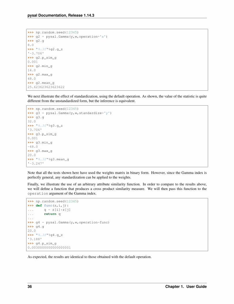
pysal Documentation, Release 1.14.3
>>> np.random.seed(12345)>>> g2 = pysal.Gamma(y,w,operation='a')>>> g2.g8.0>>> "%.3f"%g2.g_z'-3.706'>>> g2.p_sim_g0.001>>> g2.min_g14.0>>> g2.max_g48.0>>> g2.mean_g25.623623623623622
We next illustrate the effect of standardization, using the default operation. As shown, the value of the statistic is quitedifferent from the unstandardized form, but the inference is equivalent.
>>> np.random.seed(12345)>>> g3 = pysal.Gamma(y,w,standardize='y')>>> g3.g32.0>>> "%.3f"%g3.g_z'3.706'>>> g3.p_sim_g0.001>>> g3.min_g-48.0>>> g3.max_g20.0>>> "%.3f"%g3.mean_g'-3.247'
Note that all the tests shown here have used the weights matrix in binary form. However, since the Gamma index isperfectly general, any standardization can be applied to the weights.
Finally, we illustrate the use of an arbitrary attribute similarity function. In order to compare to the results above,we will define a function that produces a cross product similarity measure. We will then pass this function to theoperation argument of the Gamma index.
>>> np.random.seed(12345)>>> def func(z,i,j):... q = z[i]*z[j]... return q...>>> g4 = pysal.Gamma(y,w,operation=func)>>> g4.g20.0>>> "%.3f"%g4.g_z'3.188'>>> g4.p_sim_g0.0030000000000000001
As expected, the results are identical to those obtained with the default operation.
36 Chapter 1. User Guide
pysal Documentation, Release 1.14.3
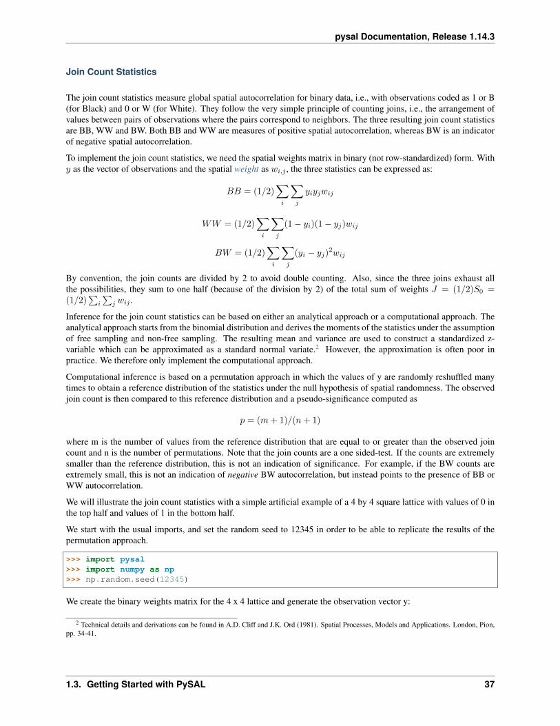
Join Count Statistics
The join count statistics measure global spatial autocorrelation for binary data, i.e., with observations coded as 1 or B(for Black) and 0 or W (for White). They follow the very simple principle of counting joins, i.e., the arrangement ofvalues between pairs of observations where the pairs correspond to neighbors. The three resulting join count statisticsare BB, WW and BW. Both BB and WW are measures of positive spatial autocorrelation, whereas BW is an indicatorof negative spatial autocorrelation.
To implement the join count statistics, we need the spatial weights matrix in binary (not row-standardized) form. With𝑦 as the vector of observations and the spatial weight as 𝑤𝑖,𝑗 , the three statistics can be expressed as:
𝐵𝐵 = (1/2)∑︁𝑖
∑︁𝑗
𝑦𝑖𝑦𝑗𝑤𝑖𝑗
𝑊𝑊 = (1/2)∑︁𝑖
∑︁𝑗
(1 − 𝑦𝑖)(1 − 𝑦𝑗)𝑤𝑖𝑗
𝐵𝑊 = (1/2)∑︁𝑖
∑︁𝑗
(𝑦𝑖 − 𝑦𝑗)2𝑤𝑖𝑗
By convention, the join counts are divided by 2 to avoid double counting. Also, since the three joins exhaust allthe possibilities, they sum to one half (because of the division by 2) of the total sum of weights 𝐽 = (1/2)𝑆0 =(1/2)
∑︀𝑖
∑︀𝑗 𝑤𝑖𝑗 .
Inference for the join count statistics can be based on either an analytical approach or a computational approach. Theanalytical approach starts from the binomial distribution and derives the moments of the statistics under the assumptionof free sampling and non-free sampling. The resulting mean and variance are used to construct a standardized z-variable which can be approximated as a standard normal variate.2 However, the approximation is often poor inpractice. We therefore only implement the computational approach.
Computational inference is based on a permutation approach in which the values of y are randomly reshuffled manytimes to obtain a reference distribution of the statistics under the null hypothesis of spatial randomness. The observedjoin count is then compared to this reference distribution and a pseudo-significance computed as
𝑝 = (𝑚 + 1)/(𝑛 + 1)
where m is the number of values from the reference distribution that are equal to or greater than the observed joincount and n is the number of permutations. Note that the join counts are a one sided-test. If the counts are extremelysmaller than the reference distribution, this is not an indication of significance. For example, if the BW counts areextremely small, this is not an indication of negative BW autocorrelation, but instead points to the presence of BB orWW autocorrelation.
We will illustrate the join count statistics with a simple artificial example of a 4 by 4 square lattice with values of 0 inthe top half and values of 1 in the bottom half.
We start with the usual imports, and set the random seed to 12345 in order to be able to replicate the results of thepermutation approach.
>>> import pysal>>> import numpy as np>>> np.random.seed(12345)
We create the binary weights matrix for the 4 x 4 lattice and generate the observation vector y:
2 Technical details and derivations can be found in A.D. Cliff and J.K. Ord (1981). Spatial Processes, Models and Applications. London, Pion,pp. 34-41.
1.3. Getting Started with PySAL 37
pysal Documentation, Release 1.14.3
>>> w=pysal.lat2W(4,4)>>> y=np.ones(16)>>> y[0:8]=0
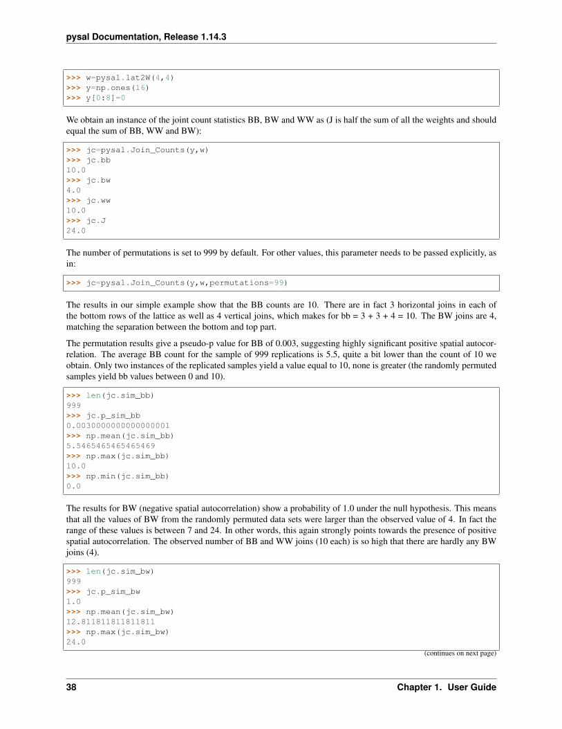
We obtain an instance of the joint count statistics BB, BW and WW as (J is half the sum of all the weights and shouldequal the sum of BB, WW and BW):
>>> jc=pysal.Join_Counts(y,w)>>> jc.bb10.0>>> jc.bw4.0>>> jc.ww10.0>>> jc.J24.0
The number of permutations is set to 999 by default. For other values, this parameter needs to be passed explicitly, asin:
>>> jc=pysal.Join_Counts(y,w,permutations=99)
The results in our simple example show that the BB counts are 10. There are in fact 3 horizontal joins in each ofthe bottom rows of the lattice as well as 4 vertical joins, which makes for bb = 3 + 3 + 4 = 10. The BW joins are 4,matching the separation between the bottom and top part.
The permutation results give a pseudo-p value for BB of 0.003, suggesting highly significant positive spatial autocor-relation. The average BB count for the sample of 999 replications is 5.5, quite a bit lower than the count of 10 weobtain. Only two instances of the replicated samples yield a value equal to 10, none is greater (the randomly permutedsamples yield bb values between 0 and 10).
>>> len(jc.sim_bb)999>>> jc.p_sim_bb0.0030000000000000001>>> np.mean(jc.sim_bb)5.5465465465465469>>> np.max(jc.sim_bb)10.0>>> np.min(jc.sim_bb)0.0
The results for BW (negative spatial autocorrelation) show a probability of 1.0 under the null hypothesis. This meansthat all the values of BW from the randomly permuted data sets were larger than the observed value of 4. In fact therange of these values is between 7 and 24. In other words, this again strongly points towards the presence of positivespatial autocorrelation. The observed number of BB and WW joins (10 each) is so high that there are hardly any BWjoins (4).
>>> len(jc.sim_bw)999>>> jc.p_sim_bw1.0>>> np.mean(jc.sim_bw)12.811811811811811>>> np.max(jc.sim_bw)24.0
(continues on next page)
38 Chapter 1. User Guide
pysal Documentation, Release 1.14.3
(continued from previous page)
>>> np.min(jc.sim_bw)7.0
Moran’s I
Moran’s I measures the global spatial autocorrelation in an attribute 𝑦 measured over 𝑛 spatial units and is given as:
𝐼 = 𝑛/𝑆0
∑︁𝑖
∑︁𝑗
𝑧𝑖𝑤𝑖,𝑗𝑧𝑗/∑︁𝑖
𝑧𝑖𝑧𝑖
where 𝑤𝑖,𝑗 is a spatial weight, 𝑧𝑖 = 𝑦𝑖− 𝑦, and 𝑆0 =∑︀
𝑖
∑︀𝑗 𝑤𝑖,𝑗 . We illustrate the use of Moran’s I with a case study
of homicide rates for a group of 78 counties surrounding St. Louis over the period 1988-93.3 We start with the usualimports:
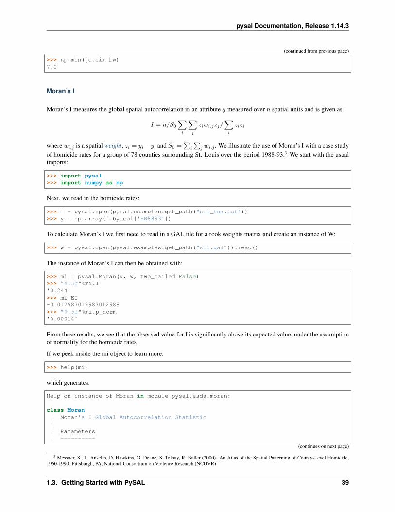
>>> import pysal>>> import numpy as np
Next, we read in the homicide rates:
>>> f = pysal.open(pysal.examples.get_path("stl_hom.txt"))>>> y = np.array(f.by_col['HR8893'])
To calculate Moran’s I we first need to read in a GAL file for a rook weights matrix and create an instance of W:
>>> w = pysal.open(pysal.examples.get_path("stl.gal")).read()
The instance of Moran’s I can then be obtained with:
>>> mi = pysal.Moran(y, w, two_tailed=False)>>> "%.3f"%mi.I'0.244'>>> mi.EI-0.012987012987012988>>> "%.5f"%mi.p_norm'0.00014'
From these results, we see that the observed value for I is significantly above its expected value, under the assumptionof normality for the homicide rates.
If we peek inside the mi object to learn more:
>>> help(mi)
which generates:
Help on instance of Moran in module pysal.esda.moran:
class Moran| Moran's I Global Autocorrelation Statistic|| Parameters| ----------
(continues on next page)
3 Messner, S., L. Anselin, D. Hawkins, G. Deane, S. Tolnay, R. Baller (2000). An Atlas of the Spatial Patterning of County-Level Homicide,1960-1990. Pittsburgh, PA, National Consortium on Violence Research (NCOVR)
1.3. Getting Started with PySAL 39
pysal Documentation, Release 1.14.3
(continued from previous page)
|| y : array| variable measured across n spatial units| w : W| spatial weights instance| permutations : int| number of random permutations for calculation of pseudo-p_values||| Attributes| ----------| y : array| original variable| w : W| original w object| permutations : int| number of permutations| I : float| value of Moran's I| EI : float| expected value under normality assumption| VI_norm : float| variance of I under normality assumption| seI_norm : float| standard deviation of I under normality assumption| z_norm : float| z-value of I under normality assumption| p_norm : float| p-value of I under normality assumption (one-sided)| for two-sided tests, this value should be multiplied by 2| VI_rand : float| variance of I under randomization assumption| seI_rand : float| standard deviation of I under randomization assumption| z_rand : float| z-value of I under randomization assumption| p_rand : float| p-value of I under randomization assumption (1-tailed)| sim : array (if permutations>0)
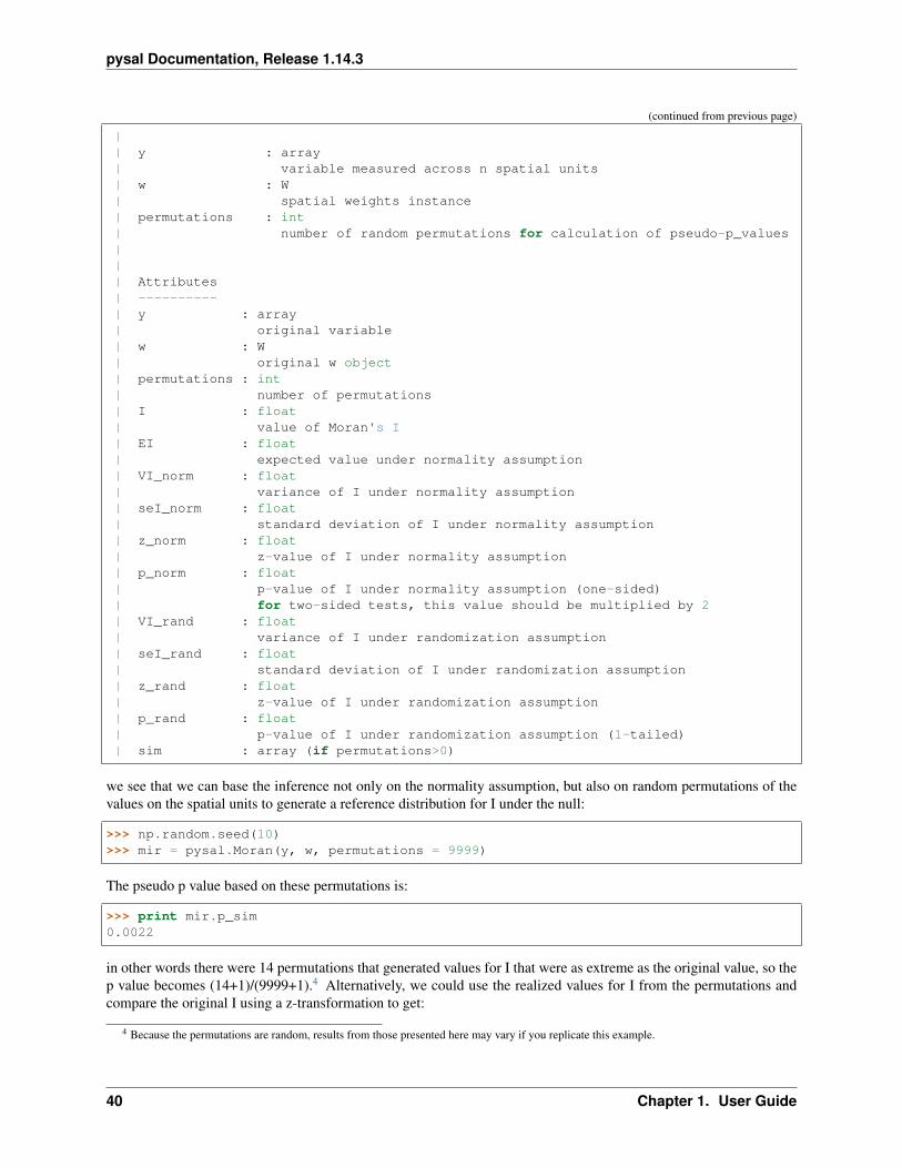
we see that we can base the inference not only on the normality assumption, but also on random permutations of thevalues on the spatial units to generate a reference distribution for I under the null:
>>> np.random.seed(10)>>> mir = pysal.Moran(y, w, permutations = 9999)
The pseudo p value based on these permutations is:
>>> print mir.p_sim0.0022
in other words there were 14 permutations that generated values for I that were as extreme as the original value, so thep value becomes (14+1)/(9999+1).4 Alternatively, we could use the realized values for I from the permutations andcompare the original I using a z-transformation to get:
4 Because the permutations are random, results from those presented here may vary if you replicate this example.
40 Chapter 1. User Guide

pysal Documentation, Release 1.14.3
>>> print mir.EI_sim-0.0118217511619>>> print mir.z_sim4.55451777821>>> print mir.p_z_sim2.62529422013e-06
When the variable of interest (𝑦) is rates based on populations with different sizes, the Moran’s I value for 𝑦 needs tobe adjusted to account for the differences among populations.5 To apply this adjustment, we can create an instanceof the Moran_Rate class rather than the Moran class. For example, let’s assume that we want to estimate the Moran’sI for the rates of newborn infants who died of Sudden Infant Death Syndrome (SIDS). We start this estimation byreading in the total number of newborn infants (BIR79) and the total number of newborn infants who died of SIDS(SID79):
>>> f = pysal.open(pysal.examples.get_path("sids2.dbf"))>>> b = np.array(f.by_col('BIR79'))>>> e = np.array(f.by_col('SID79'))
Next, we create an instance of W:
>>> w = pysal.open(pysal.examples.get_path("sids2.gal")).read()
Now, we create an instance of Moran_Rate:
>>> mi = pysal.esda.moran.Moran_Rate(e, b, w, two_tailed=False)>>> "%6.4f" % mi.I'0.1662'>>> "%6.4f" % mi.EI'-0.0101'>>> "%6.4f" % mi.p_norm'0.0042'
From these results, we see that the observed value for I is significantly higher than its expected value, after theadjustment for the differences in population.
Geary’s C
The fourth statistic for global spatial autocorrelation implemented in PySAL is Geary’s C:
𝐶 =(𝑛− 1)
2𝑆0
∑︁𝑖
∑︁𝑗
𝑤𝑖,𝑗(𝑦𝑖 − 𝑦𝑗)2/
∑︁𝑖
𝑧2𝑖
with all the terms defined as above. Applying this to the St. Louis data:
>>> np.random.seed(12345)>>> f = pysal.open(pysal.examples.get_path("stl_hom.txt"))>>> y = np.array(f.by_col['HR8893'])>>> w = pysal.open(pysal.examples.get_path("stl.gal")).read()>>> gc = pysal.Geary(y, w)>>> "%.3f"%gc.C'0.597'>>> gc.EC1.0
(continues on next page)
5 Assuncao, R. E. and Reis, E. A. 1999. A new proposal to adjust Moran’s I for population density. Statistics in Medicine. 18, 2147-2162.
1.3. Getting Started with PySAL 41
pysal Documentation, Release 1.14.3
(continued from previous page)
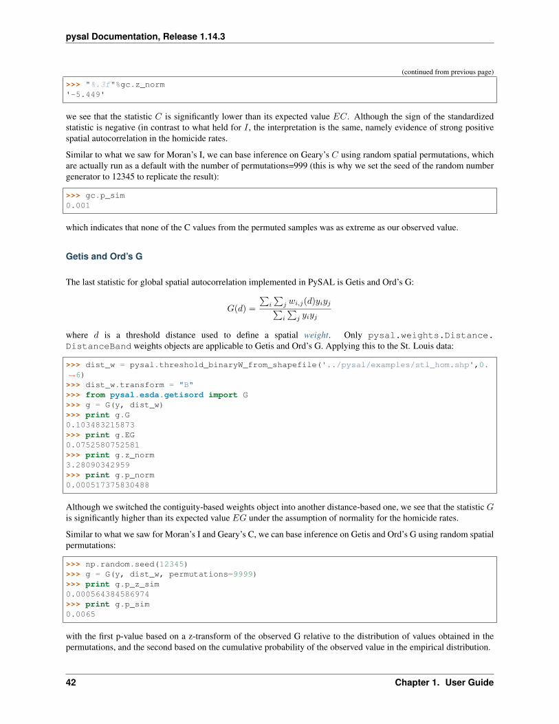
>>> "%.3f"%gc.z_norm'-5.449'
we see that the statistic 𝐶 is significantly lower than its expected value 𝐸𝐶. Although the sign of the standardizedstatistic is negative (in contrast to what held for 𝐼 , the interpretation is the same, namely evidence of strong positivespatial autocorrelation in the homicide rates.
Similar to what we saw for Moran’s I, we can base inference on Geary’s 𝐶 using random spatial permutations, whichare actually run as a default with the number of permutations=999 (this is why we set the seed of the random numbergenerator to 12345 to replicate the result):
>>> gc.p_sim0.001
which indicates that none of the C values from the permuted samples was as extreme as our observed value.
Getis and Ord’s G
The last statistic for global spatial autocorrelation implemented in PySAL is Getis and Ord’s G:
𝐺(𝑑) =
∑︀𝑖
∑︀𝑗 𝑤𝑖,𝑗(𝑑)𝑦𝑖𝑦𝑗∑︀𝑖
∑︀𝑗 𝑦𝑖𝑦𝑗
where 𝑑 is a threshold distance used to define a spatial weight. Only pysal.weights.Distance.DistanceBand weights objects are applicable to Getis and Ord’s G. Applying this to the St. Louis data:
>>> dist_w = pysal.threshold_binaryW_from_shapefile('../pysal/examples/stl_hom.shp',0.→˓6)>>> dist_w.transform = "B">>> from pysal.esda.getisord import G>>> g = G(y, dist_w)>>> print g.G0.103483215873>>> print g.EG0.0752580752581>>> print g.z_norm3.28090342959>>> print g.p_norm0.000517375830488
Although we switched the contiguity-based weights object into another distance-based one, we see that the statistic 𝐺is significantly higher than its expected value 𝐸𝐺 under the assumption of normality for the homicide rates.
Similar to what we saw for Moran’s I and Geary’s C, we can base inference on Getis and Ord’s G using random spatialpermutations:
>>> np.random.seed(12345)>>> g = G(y, dist_w, permutations=9999)>>> print g.p_z_sim0.000564384586974>>> print g.p_sim0.0065
with the first p-value based on a z-transform of the observed G relative to the distribution of values obtained in thepermutations, and the second based on the cumulative probability of the observed value in the empirical distribution.
42 Chapter 1. User Guide

pysal Documentation, Release 1.14.3
Local Autocorrelation
To measure local autocorrelation quantitatively, PySAL implements Local Indicators of Spatial Association (LISAs)for Moran’s I and Getis and Ord’s G.
Local Moran’s I
PySAL implements local Moran’s I as follows:
𝐼𝑖 =(𝑛− 1)𝑧𝑖
∑︀𝑗 𝑤𝑖,𝑗𝑧𝑗∑︀
𝑗 𝑧2𝑗
which results in 𝑛 values of local spatial autocorrelation, 1 for each spatial unit. Continuing on with the St. Louisexample, the LISA statistics are obtained with:
>>> f = pysal.open(pysal.examples.get_path("stl_hom.txt"))>>> y = np.array(f.by_col['HR8893'])>>> w = pysal.open(pysal.examples.get_path("stl.gal")).read()>>> np.random.seed(12345)>>> lm = pysal.Moran_Local(y,w)>>> lm.n78>>> len(lm.Is)78
thus we see 78 LISAs are stored in the vector lm.Is. Inference about these values is obtained through conditionalrandomization6 which leads to pseudo p-values for each LISA:
>>> lm.p_simarray([ 0.176, 0.073, 0.405, 0.267, 0.332, 0.057, 0.296, 0.242,
0.055, 0.062, 0.273, 0.488, 0.44 , 0.354, 0.415, 0.478,0.473, 0.374, 0.415, 0.21 , 0.161, 0.025, 0.338, 0.375,0.285, 0.374, 0.208, 0.3 , 0.373, 0.411, 0.478, 0.414,0.009, 0.429, 0.269, 0.015, 0.005, 0.002, 0.077, 0.001,0.088, 0.459, 0.435, 0.365, 0.231, 0.017, 0.033, 0.04 ,0.068, 0.101, 0.284, 0.309, 0.113, 0.457, 0.045, 0.269,0.118, 0.346, 0.328, 0.379, 0.342, 0.39 , 0.376, 0.467,0.357, 0.241, 0.26 , 0.401, 0.185, 0.172, 0.248, 0.4 ,0.482, 0.159, 0.373, 0.455, 0.083, 0.128])
To identify the significant7 LISA values we can use numpy indexing:
>>> sig = lm.p_sim<0.05>>> lm.p_sim[sig]array([ 0.025, 0.009, 0.015, 0.005, 0.002, 0.001, 0.017, 0.033,
0.04 , 0.045])
and then use this indexing on the q attribute to find out which quadrant of the Moran scatter plot each of the significantvalues is contained in:
>>> lm.q[sig]array([4, 1, 3, 1, 3, 1, 1, 3, 3, 3])
6 The n-1 spatial units other than i are used to generate the empirical distribution of the LISA statistics for each i.7 Caution is required in interpreting the significance of the LISA statistics due to difficulties with multiple comparisons and a lack of indepen-
dence across the individual tests. For further discussion see Anselin, L. (1995). “Local indicators of spatial association – LISA”. GeographicalAnalysis, 27, 93-115.
1.3. Getting Started with PySAL 43

pysal Documentation, Release 1.14.3
As in the case of global Moran’s I, when the variable of interest is rates based on populations with different sizes,we need to account for the differences among population to estimate local Moran’s Is. Continuing on with the SIDSexample above, the adjusted local Moran’s Is are obtained with:
>>> f = pysal.open(pysal.examples.get_path("sids2.dbf"))>>> b = np.array(f.by_col('BIR79'))>>> e = np.array(f.by_col('SID79'))>>> w = pysal.open(pysal.examples.get_path("sids2.gal")).read()
>>> np.random.seed(12345)>>> lm = pysal.esda.moran.Moran_Local_Rate(e, b, w)>>> lm.Is[:10]array([-0.13452366, -1.21133985, 0.05019761, 0.06127125, -0.12627466,
0.23497679, 0.26345855, -0.00951288, -0.01517879, -0.34513514])
As demonstrated above, significant Moran’s Is can be identified by using numpy indexing:
>>> sig = lm.p_sim<0.05>>> lm.p_sim[sig]array([ 0.021, 0.04 , 0.047, 0.015, 0.001, 0.017, 0.032, 0.031,
0.019, 0.014, 0.004, 0.048, 0.003])
Local G and G*
Getis and Ord’s G can be localized in two forms: 𝐺𝑖 and 𝐺*𝑖 .
𝐺𝑖(𝑑) =
∑︀𝑗 𝑤𝑖,𝑗(𝑑)𝑦𝑗 −𝑊𝑖𝑦(𝑖)
𝑠(𝑖){[(𝑛− 1)𝑆1𝑖 −𝑊 2𝑖 ]/(𝑛− 2)}(1/2)
, 𝑗 ̸= 𝑖
𝐺*𝑖 (𝑑) =
∑︀𝑗 𝑤𝑖,𝑗(𝑑)𝑦𝑗 −𝑊 *
𝑖 𝑦
𝑠{[(𝑛𝑆*1𝑖) − (𝑊 *
𝑖 )2]/(𝑛− 1)}(1/2), 𝑗 = 𝑖
where we have 𝑊𝑖 =∑︀
𝑗 ̸=𝑖 𝑤𝑖,𝑗(𝑑), 𝑦(𝑖) =∑︀
𝑗 𝑦𝑗
(𝑛−1) , 𝑠2(𝑖) =∑︀
𝑗 𝑦2𝑗
(𝑛−1) − [𝑦(𝑖)]2, 𝑊 *𝑖 = 𝑊𝑖+𝑤𝑖, 𝑖, 𝑆1𝑖 =
∑︀𝑗 𝑤
2𝑖,𝑗(𝑗 ̸= 𝑖),
and 𝑆*1𝑖 =
∑︀𝑗 𝑤
2𝑖,𝑗(∀𝑗), 𝑦 and 𝑠2 denote the usual sample mean and variance of 𝑦.
Continuing on with the St. Louis example, the 𝐺𝑖 and 𝐺*𝑖 statistics are obtained with:
>>> from pysal.esda.getisord import G_Local>>> np.random.seed(12345)>>> lg = G_Local(y, dist_w)>>> lg.n78>>> len(lg.Gs)78>>> lgstar = G_Local(y, dist_w, star=True)>>> lgstar.n78>>> len(lgstar.Gs)78
thus we see 78 𝐺𝑖 and 𝐺*𝑖 are stored in the vector lg.Gs and lgstar.Gs, respectively. Inference about these values is
obtained through conditional randomization as in the case of local Moran’s I:
>>> lg.p_simarray([ 0.301, 0.037, 0.457, 0.011, 0.062, 0.006, 0.094, 0.163,
0.075, 0.078, 0.419, 0.286, 0.138, 0.443, 0.36 , 0.484,
(continues on next page)
44 Chapter 1. User Guide
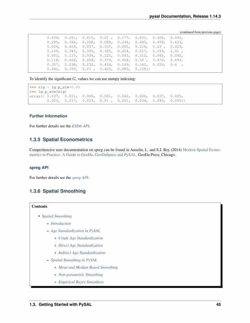
pysal Documentation, Release 1.14.3
(continued from previous page)
0.434, 0.251, 0.415, 0.21 , 0.177, 0.001, 0.304, 0.042,0.285, 0.394, 0.208, 0.089, 0.244, 0.493, 0.478, 0.433,0.006, 0.429, 0.037, 0.105, 0.005, 0.216, 0.23 , 0.023,0.105, 0.343, 0.395, 0.305, 0.264, 0.017, 0.033, 0.01 ,0.001, 0.115, 0.034, 0.225, 0.043, 0.312, 0.045, 0.092,0.118, 0.428, 0.258, 0.379, 0.408, 0.39 , 0.475, 0.493,0.357, 0.298, 0.232, 0.454, 0.149, 0.161, 0.226, 0.4 ,0.482, 0.159, 0.27 , 0.423, 0.083, 0.128])
To identify the significant 𝐺𝑖 values we can use numpy indexing:
>>> sig = lg.p_sim<0.05>>> lg.p_sim[sig]array([ 0.037, 0.011, 0.006, 0.001, 0.042, 0.006, 0.037, 0.005,
0.023, 0.017, 0.033, 0.01 , 0.001, 0.034, 0.043, 0.045])
Further Information
For further details see the ESDA API.
1.3.5 Spatial Econometrics
Comprehensive user documentation on spreg can be found in Anselin, L. and S.J. Rey (2014) Modern Spatial Econo-metrics in Practice: A Guide to GeoDa, GeoDaSpace and PySAL. GeoDa Press, Chicago.
spreg API
For further details see the spreg API.
1.3.6 Spatial Smoothing
Contents
• Spatial Smoothing
– Introduction
– Age Standardization in PySAL
* Crude Age Standardization
* Direct Age Standardization
* Indirect Age Standardization
– Spatial Smoothing in PySAL
* Mean and Median Based Smoothing
* Non-parametric Smoothing
* Empirical Bayes Smoothers
1.3. Getting Started with PySAL 45
pysal Documentation, Release 1.14.3
* Excess Risk
– Further Information
Introduction
In the spatial analysis of attributes measured for areal units, it is often necessary to transform an extensive variable,such as number of disease cases per census tract, into an intensive variable that takes into account the underlyingpopulation at risk. Raw rates, counts divided by population values, are a common standardization in the literature, yetthese tend to have unequal reliability due to different population sizes across the spatial units. This problem becomessevere for areas with small population values, since the raw rates for those areas tend to have higher variance.
A variety of spatial smoothing methods have been suggested to address this problem by aggregating the counts andpopulation values for the areas neighboring an observation and using these new measurements for its rate computation.PySAL provides a range of smoothing techniques that exploit different types of moving windows and non-parametricweighting schemes as well as the Empirical Bayesian principle. In addition, PySAL offers several methods for cal-culating age-standardized rates, since age standardization is critical in estimating rates of some events where theprobability of an event occurrence is different across different age groups.
In what follows, we overview the methods for age standardization and spatial smoothing and describe their implemen-tations in PySAL.1
Age Standardization in PySAL
Raw rates, counts divided by populations values, are based on an implicit assumption that the risk of an event isconstant over all age/sex categories in the population. For many phenomena, however, the risk is not uniform andoften highly correlated with age. To take this into account explicitly, the risks for individual age categories can beestimated separately and averaged to produce a representative value for an area.
PySAL supports three approaches to this age standardization: crude, direct, and indirect standardization.
Crude Age Standardization
In this approach, the rate for an area is simply the sum of age-specific rates weighted by the ratios of each age groupin the total population.
To obtain the rates based on this approach, we first need to create two variables that correspond to event counts andpopulation values, respectively.
>>> import numpy as np>>> e = np.array([30, 25, 25, 15, 33, 21, 30, 20])>>> b = np.array([100, 100, 110, 90, 100, 90, 110, 90])
Each set of numbers should include n by h elements where n and h are the number of areal units and the number ofage groups. In the above example there are two regions with 4 age groups. Age groups are identical across regions.The first four elements in b represent the populations of 4 age groups in the first region, and the last four elements thepopulations of the same age groups in the second region.
To apply the crude age standardization, we need to make the following function call:
1 Although this tutorial provides an introduction to the PySAL implementations for spatial smoothing, it is not exhaustive. Complete documen-tation for the implementations can be found by accessing the help from within a Python interpreter.
46 Chapter 1. User Guide

pysal Documentation, Release 1.14.3
>>> from pysal.esda import smoothing as sm>>> sm.crude_age_standardization(e, b, 2)array([ 0.2375 , 0.26666667])
In the function call above, the last argument indicates the number of area units. The outcome in the second line showsthat the age-standardized rates for two areas are about 0.24 and 0.27, respectively.
Direct Age Standardization
Direct age standardization is a variation of the crude age standardization. While crude age standardization uses theratios of each age group in the observed population, direct age standardization weights age-specific rates by the ratiosof each age group in a reference population. This reference population, the so-called standard million, is anotherrequired argument in the PySAL implementation of direct age standardization:
>>> s = np.array([100, 90, 100, 90, 100, 90, 100, 90])>>> rate = sm.direct_age_standardization(e, b, s, 2, alpha=0.05)>>> np.array(rate).round(6)array([[ 0.23744 , 0.192049, 0.290485],
[ 0.266507, 0.217714, 0.323051]])
The outcome of direct age standardization includes a set of standardized rates and their confidence intervals. Theconfidence intervals can vary according to the value for the last argument, alpha.
Indirect Age Standardization
While direct age standardization effectively addresses the variety in the risks across age groups, its indirect counterpartis better suited to handle the potential imprecision of age-specific rates due to the small population size. This methoduses age-specific rates from the standard million instead of the observed population. It then weights the rates by theratios of each age group in the observed population. To compute the age-specific rates from the standard million,the PySAL implementation of indirect age standardization requires another argument that contains the counts of theevents occurred in the standard million.
>>> s_e = np.array([10, 15, 12, 10, 5, 3, 20, 8])>>> rate = sm.indirect_age_standardization(e, b, s_e, s, 2, alpha=0.05)>>> np.array(rate).round(6)array([[ 0.208055, 0.170156, 0.254395],
[ 0.298892, 0.246631, 0.362228]])
The outcome of indirect age standardization is the same as that of its direct counterpart.
Spatial Smoothing in PySAL
Mean and Median Based Smoothing
A simple approach to rate smoothing is to find a local average or median from the rates of each observation and itsneighbors. The first method adopting this approach is the so-called locally weighted averages or disk smoother. In thismethod a rate for each observation is replaced by an average of rates for its neighbors. A spatial weights object is usedto specify the neighborhood relationships among observations. To obtain locally weighted averages of the homiciderates in the counties surrounding St. Louis during 1979-84, we first read the corresponding data table and extract datavalues for the homicide counts (the 11th column) and total population (the 13th column):
1.3. Getting Started with PySAL 47
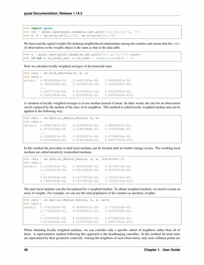
pysal Documentation, Release 1.14.3
>>> import pysal>>> stl = pysal.open(pysal.examples.get_path('stl_hom.csv'), 'r')>>> e, b = np.array(stl[:,10]), np.array(stl[:,13])
We then read the spatial weights file defining neighborhood relationships among the counties and ensure that the orderof observations in the weights object is the same as that in the data table.
>>> w = pysal.open(pysal.examples.get_path("stl.gal"),"r").read()>>> if not w.id_order_set: w.id_order = range(1,len(stl) + 1)
Now we calculate locally weighted averages of the homicide rates.
>>> rate = sm.Disk_Smoother(e, b, w)>>> rate.rarray([ 4.56502262e-05, 3.44027685e-05, 3.38280487e-05,
4.78530468e-05, 3.12278573e-05, 2.22596997e-05,...5.29577710e-05, 5.51034691e-05, 4.65160450e-05,5.32513363e-05, 3.86199097e-05, 1.92952422e-05])
A variation of locally weighted averages is to use median instead of mean. In other words, the rate for an observationcan be replaced by the median of the rates of its neighbors. This method is called locally weighted median and can beapplied in the following way:
>>> rate = sm.Spatial_Median_Rate(e, b, w)>>> rate.rarray([ 3.96047383e-05, 3.55386859e-05, 3.28308921e-05,
4.30731238e-05, 3.12453969e-05, 1.97300409e-05,...6.10668237e-05, 5.86355507e-05, 3.67396656e-05,4.82535850e-05, 5.51831429e-05, 2.99877050e-05])
In this method the procedure to find local medians can be iterated until no further change occurs. The resulting localmedians are called iteratively resmoothed medians.
>>> rate = sm.Spatial_Median_Rate(e, b, w, iteration=10)>>> rate.rarray([ 3.10194715e-05, 2.98419439e-05, 3.10194715e-05,
3.10159267e-05, 2.99214885e-05, 2.80530524e-05,...3.81364519e-05, 4.72176972e-05, 3.75320135e-05,3.76863269e-05, 4.72176972e-05, 3.75320135e-05])
The pure local medians can also be replaced by a weighted median. To obtain weighted medians, we need to create anarray of weights. For example, we can use the total population of the counties as auxiliary weights:
>>> rate = sm.Spatial_Median_Rate(e, b, w, aw=b)>>> rate.rarray([ 5.77412020e-05, 4.46449551e-05, 5.77412020e-05,
5.77412020e-05, 4.46449551e-05, 3.61363528e-05,...5.49703305e-05, 5.86355507e-05, 3.67396656e-05,3.67396656e-05, 4.72176972e-05, 2.99877050e-05])
When obtaining locally weighted medians, we can consider only a specific subset of neighbors rather than all ofthem. A representative method following this approach is the headbanging smoother. In this method all areal unitsare represented by their geometric centroids. Among the neighbors of each observation, only near collinear points are
48 Chapter 1. User Guide

pysal Documentation, Release 1.14.3
considered for median search. Then, triples of points are selected from the near collinear points, and local mediansare computed from the triples’ rates.2 We apply this headbanging smoother to the rates of the deaths from SuddenInfant Death Syndrome (SIDS) for North Carolina counties during 1974-78. We first need to read the source dataand extract the event counts (the 9th column) and population values (the 9th column). In this example the populationvalues correspond to the numbers of live births during 1974-78.
>>> sids_db = pysal.open('../pysal/examples/sids2.dbf', 'r')>>> e, b = np.array(sids_db[:,9]), np.array(sids_db[:,8])
Now we need to find triples for each observation. To support the search of triples, PySAL provides a class calledHeadbanging_Triples. This class requires an array of point observations, a spatial weights object, and the number oftriples as its arguments:
>>> from pysal import knnW>>> sids = pysal.open('../pysal/examples/sids2.shp', 'r')>>> sids_d = np.array([i.centroid for i in sids])>>> sids_w = knnW(sids_d,k=5)>>> if not sids_w.id_order_set: sids_w.id_order = sids_w.id_order>>> triples = sm.Headbanging_Triples(sids_d,sids_w,k=5)
The second line in the above example shows how to extract centroids of polygons. In this example we define 5neighbors for each observation by using nearest neighbors criteria. In the last line we define the maximum number oftriples to be found as 5.
Now we use the triples to compute the headbanging median rates:
>>> rate = sm.Headbanging_Median_Rate(e,b,triples)>>> rate.rarray([ 0.00075586, 0. , 0.0008285 , 0.0018315 , 0.00498891,
0.00482094, 0.00133156, 0.0018315 , 0.00413223, 0.00142116,...0.00221541, 0.00354767, 0.00259903, 0.00392952, 0.00207125,0.00392952, 0.00229253, 0.00392952, 0.00229253, 0.00229253])
As in the locally weighted medians, we can use a set of auxiliary weights and resmooth the medians iteratively.
Non-parametric Smoothing
Non-parametric smoothing methods compute rates without making any assumptions of distributional properties of rateestimates. A representative method in this approach is spatial filtering. PySAL provides the most simplistic form ofspatial filtering where a user-specified grid is imposed on the data set and a moving window withi a fixed or adaptiveradius visits each vertex of the grid to compute the rate at the vertex. Using the previous SIDS example, we can useSpatial_Filtering class:
>>> bbox = [sids.bbox[:2], sids.bbox[2:]]>>> rate = sm.Spatial_Filtering(bbox, sids_d, e, b, 10, 10, r=1.5)>>> rate.rarray([ 0.00152555, 0.00079271, 0.00161253, 0.00161253, 0.00139513,
0.00139513, 0.00139513, 0.00139513, 0.00139513, 0.00156348,...0.00240216, 0.00237389, 0.00240641, 0.00242211, 0.0024854 ,0.00255477, 0.00266573, 0.00288918, 0.0028991 , 0.00293492])
2 For the details of triple selection and headbanging smoothing please refer to Anselin, L., Lozano, N., and Koschinsky, J. (2006). “RateTransformations and Smoothing”. GeoDa Center Research Report.
1.3. Getting Started with PySAL 49

pysal Documentation, Release 1.14.3
The first and second arguments of the Spatial_Filtering class are a minimum bounding box containing the observationsand a set of centroids representing the observations. Be careful that the bounding box is NOT the bounding box ofthe centroids. The fifth and sixth arguments are to specify the numbers of grid cells along x and y axes. The lastargument, r, is to define the radius of the moving window. When this parameter is set, a fixed radius is applied to allgrid vertices. To make the size of moving window variable, we can specify the minimum number of population in themoving window without specifying r:
>>> rate = sm.Spatial_Filtering(bbox, sids_d, e, b, 10, 10, pop=10000)>>> rate.rarray([ 0.00157398, 0.00157398, 0.00157398, 0.00157398, 0.00166885,
0.00166885, 0.00166885, 0.00166885, 0.00166885, 0.00166885,...0.00202977, 0.00215322, 0.00207378, 0.00207378, 0.00217173,0.00232408, 0.00222717, 0.00245399, 0.00267857, 0.00267857])
The spatial rate smoother is another non-parametric smoothing method that PySAL supports. This smoother is verysimilar to the locally weighted averages. In this method, however, the weighted sum is applied to event counts and pop-ulation values separately. The resulting weighted sum of event counts is then divided by the counterpart of populationvalues. To obtain neighbor information, we need to use a spatial weights matrix as before.
>>> rate = sm.Spatial_Rate(e, b, sids_w)>>> rate.rarray([ 0.00114976, 0.00104622, 0.00110001, 0.00153257, 0.00399662,
0.00361428, 0.00146807, 0.00238521, 0.00288871, 0.00145228,...0.00240839, 0.00376101, 0.00244941, 0.0028813 , 0.00240839,0.00261705, 0.00226554, 0.0031575 , 0.00254536, 0.0029003 ])
Another variation of spatial rate smoother is kernel smoother. PySAL supports kernel smoothing by using a kernelspatial weights instance in place of a general spatial weights object.
>>> from pysal import Kernel>>> kw = Kernel(sids_d)>>> if not kw.id_order_set: kw.id_order = range(0,len(sids_d))>>> rate = sm.Kernel_Smoother(e, b, kw)>>> rate.rarray([ 0.0009831 , 0.00104298, 0.00137113, 0.00166406, 0.00556741,
0.00442273, 0.00158202, 0.00243354, 0.00282158, 0.00099243,...0.00221017, 0.00328485, 0.00257988, 0.00370461, 0.0020566 ,0.00378135, 0.00240358, 0.00432019, 0.00227857, 0.00251648])
Age-adjusted rate smoother is another non-parametric smoother that PySAL provides. This smoother applies directage standardization while computing spatial rates. To illustrate the age-adjusted rate smoother, we create a new set ofevent counts and population values as well as a new kernel weights object.
>>> e = np.array([10, 8, 1, 4, 3, 5, 4, 3, 2, 1, 5, 3])>>> b = np.array([100, 90, 15, 30, 25, 20, 30, 20, 80, 80, 90, 60])>>> s = np.array([98, 88, 15, 29, 20, 23, 33, 25, 76, 80, 89, 66])>>> points=[(10, 10), (20, 10), (40, 10), (15, 20), (30, 20), (30, 30)]>>> kw=Kernel(points)>>> if not kw.id_order_set: kw.id_order = range(0,len(points))
In the above example we created 6 observations each of which has two age groups. To apply age-adjusted ratesmoothing, we use the Age_Adjusted_Smoother class as follows:
50 Chapter 1. User Guide

pysal Documentation, Release 1.14.3
>>> rate = sm.Age_Adjusted_Smoother(e, b, kw, s)>>> rate.rarray([ 0.10519625, 0.08494318, 0.06440072, 0.06898604, 0.06952076,
0.05020968])
Empirical Bayes Smoothers
The last group of smoothing methods that PySAL supports is based upon the Bayesian principle. These methodsadjust a raw rate by taking into account information in the other raw rates. As a reference PySAL provides a methodfor a-spatial Empirical Bayes smoothing:
>>> e, b = sm.sum_by_n(e, np.ones(12), 6), sm.sum_by_n(b, np.ones(12), 6)>>> rate = sm.Empirical_Bayes(e, b)>>> rate.rarray([ 0.09080775, 0.09252352, 0.12332267, 0.10753624, 0.03301368,
0.05934766])
In the first line of the above example we aggregate the event counts and population values by observation. Next weapplied the Empirical_Bayes class to the aggregated counts and population values.
A spatial Empirical Bayes smoother is also implemented in PySAL. This method requires an additional argument, i.e.,a spatial weights object. We continue to reuse the kernel spatial weights object we built before.
>>> rate = sm.Spatial_Empirical_Bayes(e, b, kw)>>> rate.rarray([ 0.10105263, 0.10165261, 0.16104362, 0.11642038, 0.0226908 ,
0.05270639])
Excess Risk
Besides a variety of spatial smoothing methods, PySAL provides a class for estimating excess risk from event countsand population values. Excess risks are the ratios of observed event counts over expected event counts. An examplefor the class usage is as follows:
>>> risk = sm.Excess_Risk(e, b)>>> risk.rarray([ 1.23737916, 1.45124717, 2.32199546, 1.82857143, 0.24489796,
0.69659864])
Further Information
For further details see the Smoothing API.
1.3.7 Regionalization
Introduction
PySAL offers a number of tools for the construction of regions. For the purposes of this section, a “region” is a groupof “areas,” and there are generally multiple regions in a particular dataset. At this time, PySAL offers the max-pregionalization algorithm and tools for constructing random regions.
1.3. Getting Started with PySAL 51

pysal Documentation, Release 1.14.3
max-p
Most regionalization algorithms require the user to define a priori the number of regions to be built (e.g. k-meansclustering). The max-p algorithm1 determines the number of regions (p) endogenously based on a set of areas, amatrix of attributes on each area and a floor constraint. The floor constraint defines the minimum bound that a variablemust reach for each region; for example, a constraint might be the minimum population each region must have. max-pfurther enforces a contiguity constraint on the areas within regions.
To illustrate this we will use data on per capita income from the lower 48 US states over the period 1929-2010. Thegoal is to form contiguous regions of states displaying similar levels of income throughout this period:
>>> import pysal>>> import numpy as np>>> import random>>> f = pysal.open("../pysal/examples/usjoin.csv")>>> pci = np.array([f.by_col[str(y)] for y in range(1929, 2010)])>>> pci = pci.transpose()>>> pci.shape(48, 81)
We also require set of binary contiguity weights for the Maxp class:
>>> w = pysal.open("../pysal/examples/states48.gal").read()
Once we have the attribute data and our weights object we can create an instance of Maxp:
>>> np.random.seed(100)>>> random.seed(10)>>> r = pysal.Maxp(w, pci, floor = 5, floor_variable = np.ones((48, 1)), initial = 99)
Here we are forming regions with a minimum of 5 states in each region, so we set the floor_variable to a simple unitvector to ensure this floor constraint is satisfied. We also specify the initial number of feasible solutions to 99 - whichare then searched over to pick the optimal feasible solution to then commence with the more expensive swappingcomponent of the algorithm.2
The Maxp instance s has a number of attributes regarding the solution. First is the definition of the regions:
>>> r.regions[['44', '34', '3', '25', '1', '4', '47'], ['12', '46', '20', '24', '13'], ['14', '45',→˓ '35', '30', '39'], ['6', '27', '17', '29', '5', '43'], ['33', '40', '28', '15', '41→˓', '9', '23', '31', '38'], ['37', '8', '0', '7', '21', '2'], ['32', '19', '11', '10→˓', '22'], ['16', '26', '42', '18', '36']]
which is a list of eight lists of region ids. For example, the first nested list indicates there are seven states in the firstregion, while the last region has five states. To determine which states these are we can read in the names from theoriginal csv file:
>>> f.header['Name', 'STATE_FIPS', '1929', '1930', '1931', '1932', '1933', '1934', '1935', '1936',→˓ '1937', '1938', '1939', '1940', '1941', '1942', '1943', '1944', '1945', '1946',→˓'1947', '1948', '1949', '1950', '1951', '1952', '1953', '1954', '1955', '1956',→˓'1957', '1958', '1959', '1960', '1961', '1962', '1963', '1964', '1965', '1966',→˓'1967', '1968', '1969', '1970', '1971', '1972', '1973', '1974', '1975', '1976',→˓'1977', '1978', '1979', '1980', '1981', '1982', '1983', '1984', '1985', '1986',→˓'1987', '1988', '1989', '1990', '1991', '1992', '1993', '1994', '1995', '1996',→˓'1997', '1998', '1999', '2000', '2001', '2002', '2003', '2004', '2005', '2006',→˓'2007', '2008', '2009']
(continues on next page)
1 Duque, J. C., L. Anselin and S. J. Rey. 2011. “The max-p-regions problem.” Journal of Regional Science DOI: 10.1111/j.1467-9787.2011.00743.x
2 Because this is a randomized algorithm, results may vary when replicating this example. To reproduce a regionalization solution, you shouldfirst set the random seed generator. See http://docs.scipy.org/doc/numpy/reference/generated/numpy.random.seed.html for more information.
52 Chapter 1. User Guide

pysal Documentation, Release 1.14.3
(continued from previous page)
>>> names = f.by_col('Name')>>> names = np.array(names)>>> print names['Alabama' 'Arizona' 'Arkansas' 'California' 'Colorado' 'Connecticut''Delaware' 'Florida' 'Georgia' 'Idaho' 'Illinois' 'Indiana' 'Iowa''Kansas' 'Kentucky' 'Louisiana' 'Maine' 'Maryland' 'Massachusetts''Michigan' 'Minnesota' 'Mississippi' 'Missouri' 'Montana' 'Nebraska''Nevada' 'New Hampshire' 'New Jersey' 'New Mexico' 'New York''North Carolina' 'North Dakota' 'Ohio' 'Oklahoma' 'Oregon' 'Pennsylvania''Rhode Island' 'South Carolina' 'South Dakota' 'Tennessee' 'Texas' 'Utah''Vermont' 'Virginia' 'Washington' 'West Virginia' 'Wisconsin' 'Wyoming']
and then loop over the region definitions to identify the specific states comprising each of the regions:
>>> for region in r.regions:... ids = map(int,region)... print names[ids]...['Washington' 'Oregon' 'California' 'Nevada' 'Arizona' 'Colorado' 'Wyoming']['Iowa' 'Wisconsin' 'Minnesota' 'Nebraska' 'Kansas']['Kentucky' 'West Virginia' 'Pennsylvania' 'North Carolina' 'Tennessee']['Delaware' 'New Jersey' 'Maryland' 'New York' 'Connecticut' 'Virginia']['Oklahoma' 'Texas' 'New Mexico' 'Louisiana' 'Utah' 'Idaho' 'Montana''North Dakota' 'South Dakota']
['South Carolina' 'Georgia' 'Alabama' 'Florida' 'Mississippi' 'Arkansas']['Ohio' 'Michigan' 'Indiana' 'Illinois' 'Missouri']['Maine' 'New Hampshire' 'Vermont' 'Massachusetts' 'Rhode Island']
We can evaluate our solution by developing a pseudo pvalue for the regionalization. This is done by comparing thewithin region sum of squares for the solution against simulated solutions where areas are randomly assigned to regionsthat maintain the cardinality of the original solution. This method must be explicitly called once the Maxp instancehas been created:
>>> r.inference()>>> r.pvalue0.01
so we see we have a regionalization that is significantly different than a chance partitioning.
Random Regions
PySAL offers functionality to generate random regions based on user-defined constraints. There are three optionalparameters to constrain the regionalization: number of regions, cardinality and contiguity. The default case simplytakes a list of area IDs and randomly selects the number of regions and then allocates areas to each region. The usercan also pass a vector of integers to the cardinality parameter to designate the number of areas to randomly assign toeach region. The contiguity parameter takes a spatial weights object and uses that to ensure that each region is made upof spatially contiguous areas. When the contiguity constraint is enforced, it is possible to arrive at infeasible solutions;the maxiter parameter can be set to make multiple attempts to find a feasible solution. The following examples showsome of the possible combinations of constraints.
>>> import random>>> import numpy as np>>> import pysal>>> from pysal.region import Random_Region
(continues on next page)
1.3. Getting Started with PySAL 53
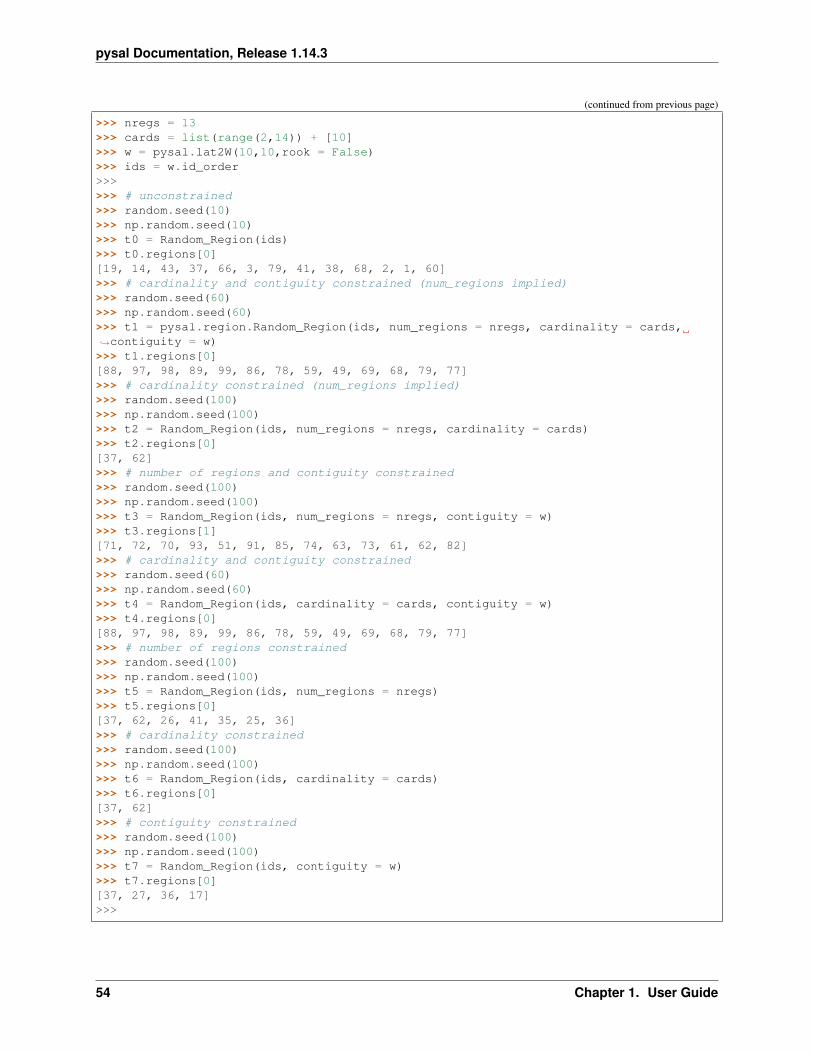
pysal Documentation, Release 1.14.3
(continued from previous page)
>>> nregs = 13>>> cards = list(range(2,14)) + [10]>>> w = pysal.lat2W(10,10,rook = False)>>> ids = w.id_order>>>>>> # unconstrained>>> random.seed(10)>>> np.random.seed(10)>>> t0 = Random_Region(ids)>>> t0.regions[0][19, 14, 43, 37, 66, 3, 79, 41, 38, 68, 2, 1, 60]>>> # cardinality and contiguity constrained (num_regions implied)>>> random.seed(60)>>> np.random.seed(60)>>> t1 = pysal.region.Random_Region(ids, num_regions = nregs, cardinality = cards,→˓contiguity = w)>>> t1.regions[0][88, 97, 98, 89, 99, 86, 78, 59, 49, 69, 68, 79, 77]>>> # cardinality constrained (num_regions implied)>>> random.seed(100)>>> np.random.seed(100)>>> t2 = Random_Region(ids, num_regions = nregs, cardinality = cards)>>> t2.regions[0][37, 62]>>> # number of regions and contiguity constrained>>> random.seed(100)>>> np.random.seed(100)>>> t3 = Random_Region(ids, num_regions = nregs, contiguity = w)>>> t3.regions[1][71, 72, 70, 93, 51, 91, 85, 74, 63, 73, 61, 62, 82]>>> # cardinality and contiguity constrained>>> random.seed(60)>>> np.random.seed(60)>>> t4 = Random_Region(ids, cardinality = cards, contiguity = w)>>> t4.regions[0][88, 97, 98, 89, 99, 86, 78, 59, 49, 69, 68, 79, 77]>>> # number of regions constrained>>> random.seed(100)>>> np.random.seed(100)>>> t5 = Random_Region(ids, num_regions = nregs)>>> t5.regions[0][37, 62, 26, 41, 35, 25, 36]>>> # cardinality constrained>>> random.seed(100)>>> np.random.seed(100)>>> t6 = Random_Region(ids, cardinality = cards)>>> t6.regions[0][37, 62]>>> # contiguity constrained>>> random.seed(100)>>> np.random.seed(100)>>> t7 = Random_Region(ids, contiguity = w)>>> t7.regions[0][37, 27, 36, 17]>>>
54 Chapter 1. User Guide

pysal Documentation, Release 1.14.3
Further Information
For further details see the Regionalization API.
1.3.8 Spatial Dynamics
Contents
• Spatial Dynamics
– Introduction
– Markov Based Methods
* Classic Markov
* Spatial Markov
* LISA Markov
– Rank Based Methods
* Spatial Rank Correlation
* Rank Decomposition
– Space-Time Interaction Tests
* Knox Test
* Modified Knox Test
* Mantel Test
* Jacquez Test
– Spatial Dynamics API
Introduction
PySAL implements a number of exploratory approaches to analyze the dynamics of longitudinal spatial data, orobservations on fixed areal units over multiple time periods. Examples could include time series of voting patternsin US Presidential elections, time series of remote sensing images, labor market dynamics, regional business cycles,among many others. Two broad sets of spatial dynamics methods are implemented to analyze these data types. Thefirst are Markov based methods, while the second are based on Rank dynamics.
Additionally, methods are included in this module to analyze patterns of individual events which have spatial andtemporal coordinates associated with them. Examples include locations and times of individual cases of disease orcrimes. Methods are included here to determine if these event patterns exhibit space-time interaction.
Markov Based Methods
The Markov based methods include classic Markov chains and extensions of these approaches to deal with spatiallyreferenced data. In what follows we illustrate the functionality of these Markov methods. Readers interested in themethodological foundations of these approaches are directed to1.
1 Rey, S.J. 2001. “Spatial empirics for economic growth and convergence”, 34 Geographical Analysis, 33, 195-214.
1.3. Getting Started with PySAL 55
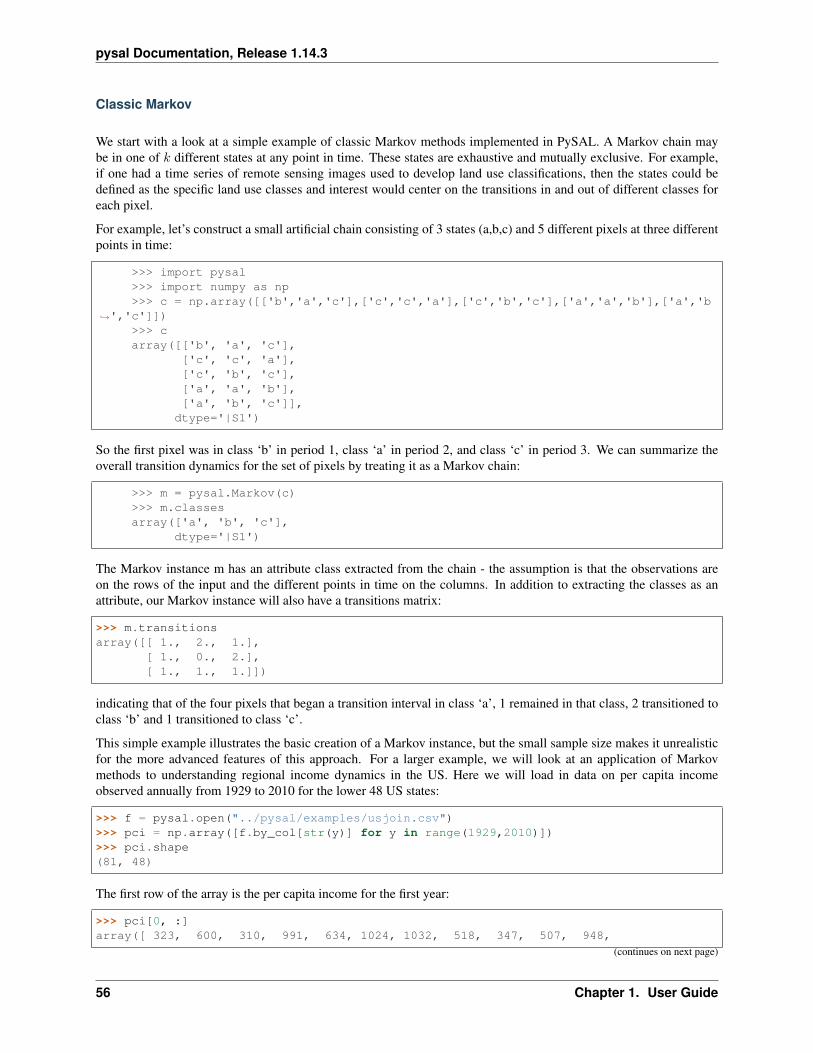
pysal Documentation, Release 1.14.3
Classic Markov
We start with a look at a simple example of classic Markov methods implemented in PySAL. A Markov chain maybe in one of 𝑘 different states at any point in time. These states are exhaustive and mutually exclusive. For example,if one had a time series of remote sensing images used to develop land use classifications, then the states could bedefined as the specific land use classes and interest would center on the transitions in and out of different classes foreach pixel.
For example, let’s construct a small artificial chain consisting of 3 states (a,b,c) and 5 different pixels at three differentpoints in time:
>>> import pysal>>> import numpy as np>>> c = np.array([['b','a','c'],['c','c','a'],['c','b','c'],['a','a','b'],['a','b
→˓','c']])>>> carray([['b', 'a', 'c'],
['c', 'c', 'a'],['c', 'b', 'c'],['a', 'a', 'b'],['a', 'b', 'c']],
dtype='|S1')
So the first pixel was in class ‘b’ in period 1, class ‘a’ in period 2, and class ‘c’ in period 3. We can summarize theoverall transition dynamics for the set of pixels by treating it as a Markov chain:
>>> m = pysal.Markov(c)>>> m.classesarray(['a', 'b', 'c'],
dtype='|S1')
The Markov instance m has an attribute class extracted from the chain - the assumption is that the observations areon the rows of the input and the different points in time on the columns. In addition to extracting the classes as anattribute, our Markov instance will also have a transitions matrix:
>>> m.transitionsarray([[ 1., 2., 1.],
[ 1., 0., 2.],[ 1., 1., 1.]])
indicating that of the four pixels that began a transition interval in class ‘a’, 1 remained in that class, 2 transitioned toclass ‘b’ and 1 transitioned to class ‘c’.
This simple example illustrates the basic creation of a Markov instance, but the small sample size makes it unrealisticfor the more advanced features of this approach. For a larger example, we will look at an application of Markovmethods to understanding regional income dynamics in the US. Here we will load in data on per capita incomeobserved annually from 1929 to 2010 for the lower 48 US states:
>>> f = pysal.open("../pysal/examples/usjoin.csv")>>> pci = np.array([f.by_col[str(y)] for y in range(1929,2010)])>>> pci.shape(81, 48)
The first row of the array is the per capita income for the first year:
>>> pci[0, :]array([ 323, 600, 310, 991, 634, 1024, 1032, 518, 347, 507, 948,
(continues on next page)
56 Chapter 1. User Guide

pysal Documentation, Release 1.14.3
(continued from previous page)
607, 581, 532, 393, 414, 601, 768, 906, 790, 599, 286,621, 592, 596, 868, 686, 918, 410, 1152, 332, 382, 771,455, 668, 772, 874, 271, 426, 378, 479, 551, 634, 434,741, 460, 673, 675])
In order to apply the classic Markov approach to this series, we first have to discretize the distribution by definingour classes. There are many ways to do this, but here we will use the quintiles for each annual income distribution todefine the classes:
>>> q5 = np.array([pysal.Quantiles(y).yb for y in pci]).transpose()>>> q5.shape(48, 81)>>> q5[:, 0]array([0, 2, 0, 4, 2, 4, 4, 1, 0, 1, 4, 2, 2, 1, 0, 1, 2, 3, 4, 4, 2, 0, 2,
2, 2, 4, 3, 4, 0, 4, 0, 0, 3, 1, 3, 3, 4, 0, 1, 0, 1, 2, 2, 1, 3, 1,3, 3])
A number of things need to be noted here. First, we are relying on the classification methods in PySAL for definingour quintiles. The class Quantiles uses quintiles as the default and will create an instance of this class that has multipleattributes, the one we are extracting in the first line is yb - the class id for each observation. The second thing to noteis the transpose operator which gets our resulting array q5 in the proper structure required for use of Markov. Thuswe see that the first spatial unit (Alabama with an income of 323) fell in the first quintile in 1929, while the last unit(Wyoming with an income of 675) fell in the fourth quintile2.
So now we have a time series for each state of its quintile membership. For example, Colorado’s quintile time seriesis:
>>> q5[4, :]array([2, 3, 2, 2, 3, 2, 2, 3, 2, 2, 2, 2, 2, 2, 2, 2, 3, 2, 3, 2, 3, 2, 3,
3, 3, 2, 2, 3, 3, 3, 3, 3, 3, 3, 3, 3, 3, 2, 2, 2, 3, 3, 3, 3, 3, 3,3, 3, 3, 3, 3, 4, 4, 4, 4, 4, 4, 3, 3, 3, 3, 3, 3, 3, 3, 3, 4, 4, 4,4, 4, 4, 4, 4, 3, 3, 3, 4, 3, 3, 3])
indicating that it has occupied the 3rd, 4th and 5th quintiles in the distribution at different points in time. To summarizethe transition dynamics for all units, we instantiate a Markov object:
>>> m5 = pysal.Markov(q5)>>> m5.transitionsarray([[ 729., 71., 1., 0., 0.],
[ 72., 567., 80., 3., 0.],[ 0., 81., 631., 86., 2.],[ 0., 3., 86., 573., 56.],[ 0., 0., 1., 57., 741.]])
Assuming we can treat these transitions as a first order Markov chain, we can estimate the transition probabilities:
>>> m5.pmatrix([[ 0.91011236, 0.0886392 , 0.00124844, 0. , 0. ],
[ 0.09972299, 0.78531856, 0.11080332, 0.00415512, 0. ],[ 0. , 0.10125 , 0.78875 , 0.1075 , 0.0025 ],[ 0. , 0.00417827, 0.11977716, 0.79805014, 0.07799443],[ 0. , 0. , 0.00125156, 0.07133917, 0.92740926]])
as well as the long run steady state distribution:2 The states are ordered alphabetically.
1.3. Getting Started with PySAL 57

pysal Documentation, Release 1.14.3
>>> m5.steady_statematrix([[ 0.20774716],
[ 0.18725774],[ 0.20740537],[ 0.18821787],[ 0.20937187]])
With the transition probability matrix in hand, we can estimate the first mean passage time:
>>> pysal.ergodic.fmpt(m5.p)matrix([[ 4.81354357, 11.50292712, 29.60921231, 53.38594954,
103.59816743],[ 42.04774505, 5.34023324, 18.74455332, 42.50023268,
92.71316899],[ 69.25849753, 27.21075248, 4.82147603, 25.27184624,
75.43305672],[ 84.90689329, 42.85914824, 17.18082642, 5.31299186,
51.60953369],[ 98.41295543, 56.36521038, 30.66046735, 14.21158356,
4.77619083]])
Thus, for a state with income in the first quintile, it takes on average 11.5 years for it to first enter the second quintile,29.6 to get to the third quintile, 53.4 years to enter the fourth, and 103.6 years to reach the richest quintile.
Spatial Markov
Thus far we have treated all the spatial units as independent to estimate the transition probabilities. This hides anumber of implicit assumptions. First, the transition dynamics are assumed to hold for all units and for all timeperiods. Second, interactions between the transitions of individual units are ignored. In other words regional contextmay be important to understand regional income dynamics, but the classic Markov approach is silent on this issue.
PySAL includes a number of spatially explicit extensions to the Markov framework. The first is the spatial Markovclass that we illustrate here. We first are going to transform the income series to relative incomes (by standardizing byeach period by the mean):
>>> import pysal>>> f = pysal.open("../pysal/examples/usjoin.csv")>>> pci = np.array([f.by_col[str(y)] for y in range(1929, 2010)])>>> pci = pci.transpose()>>> rpci = pci / (pci.mean(axis = 0))
Next, we require a spatial weights object, and here we will create one from an external GAL file:
>>> w = pysal.open("../pysal/examples/states48.gal").read()>>> w.transform = 'r'
Finally, we create an instance of the Spatial Markov class using 5 states for the chain:
>>> sm = pysal.Spatial_Markov(rpci, w, fixed = True, k = 5)
Here we are keeping the quintiles fixed, meaning the data are pooled over space and time and the quintiles calculatedfor the pooled data. This is why we first transformed the data to relative incomes. We can next examine the globaltransition probability matrix for relative incomes:
58 Chapter 1. User Guide
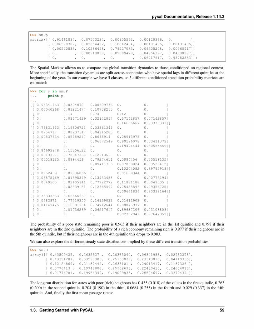
pysal Documentation, Release 1.14.3
>>> sm.pmatrix([[ 0.91461837, 0.07503234, 0.00905563, 0.00129366, 0. ],
[ 0.06570302, 0.82654402, 0.10512484, 0.00131406, 0.00131406],[ 0.00520833, 0.10286458, 0.79427083, 0.09505208, 0.00260417],[ 0. , 0.00913838, 0.09399478, 0.84856397, 0.04830287],[ 0. , 0. , 0. , 0.06217617, 0.93782383]])
The Spatial Markov allows us to compare the global transition dynamics to those conditioned on regional context.More specifically, the transition dynamics are split across economies who have spatial lags in different quintiles at thebeginning of the year. In our example we have 5 classes, so 5 different conditioned transition probability matrices areestimated:
>>> for p in sm.P:... print p...[[ 0.96341463 0.0304878 0.00609756 0. 0. ][ 0.06040268 0.83221477 0.10738255 0. 0. ][ 0. 0.14 0.74 0.12 0. ][ 0. 0.03571429 0.32142857 0.57142857 0.07142857][ 0. 0. 0. 0.16666667 0.83333333]]
[[ 0.79831933 0.16806723 0.03361345 0. 0. ][ 0.0754717 0.88207547 0.04245283 0. 0. ][ 0.00537634 0.06989247 0.8655914 0.05913978 0. ][ 0. 0. 0.06372549 0.90196078 0.03431373][ 0. 0. 0. 0.19444444 0.80555556]]
[[ 0.84693878 0.15306122 0. 0. 0. ][ 0.08133971 0.78947368 0.1291866 0. 0. ][ 0.00518135 0.0984456 0.79274611 0.0984456 0.00518135][ 0. 0. 0.09411765 0.87058824 0.03529412][ 0. 0. 0. 0.10204082 0.89795918]]
[[ 0.8852459 0.09836066 0. 0.01639344 0. ][ 0.03875969 0.81395349 0.13953488 0. 0.00775194][ 0.0049505 0.09405941 0.77722772 0.11881188 0.0049505 ][ 0. 0.02339181 0.12865497 0.75438596 0.09356725][ 0. 0. 0. 0.09661836 0.90338164]]
[[ 0.33333333 0.66666667 0. 0. 0. ][ 0.0483871 0.77419355 0.16129032 0.01612903 0. ][ 0.01149425 0.16091954 0.74712644 0.08045977 0. ][ 0. 0.01036269 0.06217617 0.89637306 0.03108808][ 0. 0. 0. 0.02352941 0.97647059]]
The probability of a poor state remaining poor is 0.963 if their neighbors are in the 1st quintile and 0.798 if theirneighbors are in the 2nd quintile. The probability of a rich economy remaining rich is 0.977 if their neighbors are inthe 5th quintile, but if their neighbors are in the 4th quintile this drops to 0.903.
We can also explore the different steady state distributions implied by these different transition probabilities:
>>> sm.Sarray([[ 0.43509425, 0.2635327 , 0.20363044, 0.06841983, 0.02932278],
[ 0.13391287, 0.33993305, 0.25153036, 0.23343016, 0.04119356],[ 0.12124869, 0.21137444, 0.2635101 , 0.29013417, 0.1137326 ],[ 0.0776413 , 0.19748806, 0.25352636, 0.22480415, 0.24654013],[ 0.01776781, 0.19964349, 0.19009833, 0.25524697, 0.3372434 ]])
The long run distribution for states with poor (rich) neighbors has 0.435 (0.018) of the values in the first quintile, 0.263(0.200) in the second quintile, 0.204 (0.190) in the third, 0.0684 (0.255) in the fourth and 0.029 (0.337) in the fifthquintile. And, finally the first mean passage times:
1.3. Getting Started with PySAL 59
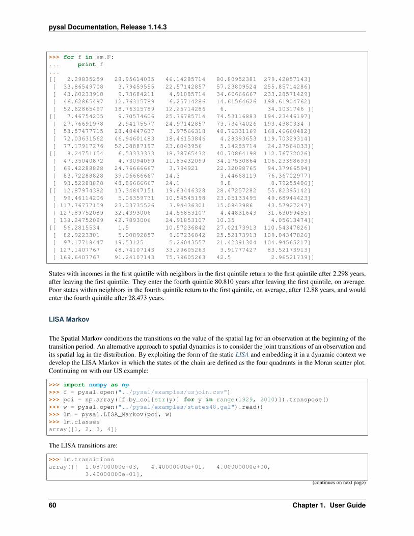
pysal Documentation, Release 1.14.3
>>> for f in sm.F:... print f...[[ 2.29835259 28.95614035 46.14285714 80.80952381 279.42857143][ 33.86549708 3.79459555 22.57142857 57.23809524 255.85714286][ 43.60233918 9.73684211 4.91085714 34.66666667 233.28571429][ 46.62865497 12.76315789 6.25714286 14.61564626 198.61904762][ 52.62865497 18.76315789 12.25714286 6. 34.1031746 ]]
[[ 7.46754205 9.70574606 25.76785714 74.53116883 194.23446197][ 27.76691978 2.94175577 24.97142857 73.73474026 193.4380334 ][ 53.57477715 28.48447637 3.97566318 48.76331169 168.46660482][ 72.03631562 46.94601483 18.46153846 4.28393653 119.70329314][ 77.17917276 52.08887197 23.6043956 5.14285714 24.27564033]]
[[ 8.24751154 6.53333333 18.38765432 40.70864198 112.76732026][ 47.35040872 4.73094099 11.85432099 34.17530864 106.23398693][ 69.42288828 24.76666667 3.794921 22.32098765 94.37966594][ 83.72288828 39.06666667 14.3 3.44668119 76.36702977][ 93.52288828 48.86666667 24.1 9.8 8.79255406]]
[[ 12.87974382 13.34847151 19.83446328 28.47257282 55.82395142][ 99.46114206 5.06359731 10.54545198 23.05133495 49.68944423][ 117.76777159 23.03735526 3.94436301 15.0843986 43.57927247][ 127.89752089 32.4393006 14.56853107 4.44831643 31.63099455][ 138.24752089 42.7893006 24.91853107 10.35 4.05613474]]
[[ 56.2815534 1.5 10.57236842 27.02173913 110.54347826][ 82.9223301 5.00892857 9.07236842 25.52173913 109.04347826][ 97.17718447 19.53125 5.26043557 21.42391304 104.94565217][ 127.1407767 48.74107143 33.29605263 3.91777427 83.52173913][ 169.6407767 91.24107143 75.79605263 42.5 2.96521739]]
States with incomes in the first quintile with neighbors in the first quintile return to the first quintile after 2.298 years,after leaving the first quintile. They enter the fourth quintile 80.810 years after leaving the first quintile, on average.Poor states within neighbors in the fourth quintile return to the first quintile, on average, after 12.88 years, and wouldenter the fourth quintile after 28.473 years.
LISA Markov
The Spatial Markov conditions the transitions on the value of the spatial lag for an observation at the beginning of thetransition period. An alternative approach to spatial dynamics is to consider the joint transitions of an observation andits spatial lag in the distribution. By exploiting the form of the static LISA and embedding it in a dynamic context wedevelop the LISA Markov in which the states of the chain are defined as the four quadrants in the Moran scatter plot.Continuing on with our US example:
>>> import numpy as np>>> f = pysal.open("../pysal/examples/usjoin.csv")>>> pci = np.array([f.by_col[str(y)] for y in range(1929, 2010)]).transpose()>>> w = pysal.open("../pysal/examples/states48.gal").read()>>> lm = pysal.LISA_Markov(pci, w)>>> lm.classesarray([1, 2, 3, 4])
The LISA transitions are:
>>> lm.transitionsarray([[ 1.08700000e+03, 4.40000000e+01, 4.00000000e+00,
3.40000000e+01],
(continues on next page)
60 Chapter 1. User Guide
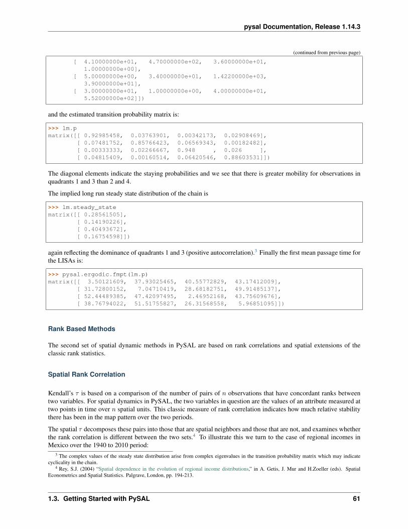
pysal Documentation, Release 1.14.3
(continued from previous page)
[ 4.10000000e+01, 4.70000000e+02, 3.60000000e+01,1.00000000e+00],
[ 5.00000000e+00, 3.40000000e+01, 1.42200000e+03,3.90000000e+01],
[ 3.00000000e+01, 1.00000000e+00, 4.00000000e+01,5.52000000e+02]])
and the estimated transition probability matrix is:
>>> lm.pmatrix([[ 0.92985458, 0.03763901, 0.00342173, 0.02908469],
[ 0.07481752, 0.85766423, 0.06569343, 0.00182482],[ 0.00333333, 0.02266667, 0.948 , 0.026 ],[ 0.04815409, 0.00160514, 0.06420546, 0.88603531]])
The diagonal elements indicate the staying probabilities and we see that there is greater mobility for observations inquadrants 1 and 3 than 2 and 4.
The implied long run steady state distribution of the chain is
>>> lm.steady_statematrix([[ 0.28561505],
[ 0.14190226],[ 0.40493672],[ 0.16754598]])
again reflecting the dominance of quadrants 1 and 3 (positive autocorrelation).3 Finally the first mean passage time forthe LISAs is:
>>> pysal.ergodic.fmpt(lm.p)matrix([[ 3.50121609, 37.93025465, 40.55772829, 43.17412009],
[ 31.72800152, 7.04710419, 28.68182751, 49.91485137],[ 52.44489385, 47.42097495, 2.46952168, 43.75609676],[ 38.76794022, 51.51755827, 26.31568558, 5.96851095]])
Rank Based Methods
The second set of spatial dynamic methods in PySAL are based on rank correlations and spatial extensions of theclassic rank statistics.
Spatial Rank Correlation
Kendall’s 𝜏 is based on a comparison of the number of pairs of 𝑛 observations that have concordant ranks betweentwo variables. For spatial dynamics in PySAL, the two variables in question are the values of an attribute measured attwo points in time over 𝑛 spatial units. This classic measure of rank correlation indicates how much relative stabilitythere has been in the map pattern over the two periods.
The spatial 𝜏 decomposes these pairs into those that are spatial neighbors and those that are not, and examines whetherthe rank correlation is different between the two sets.4 To illustrate this we turn to the case of regional incomes inMexico over the 1940 to 2010 period:
3 The complex values of the steady state distribution arise from complex eigenvalues in the transition probability matrix which may indicatecyclicality in the chain.
4 Rey, S.J. (2004) “Spatial dependence in the evolution of regional income distributions,” in A. Getis, J. Mur and H.Zoeller (eds). SpatialEconometrics and Spatial Statistics. Palgrave, London, pp. 194-213.
1.3. Getting Started with PySAL 61

pysal Documentation, Release 1.14.3
>>> import pysal>>> f = pysal.open("../pysal/examples/mexico.csv")>>> vnames = ["pcgdp%d"%dec for dec in range(1940, 2010, 10)]>>> y = np.transpose(np.array([f.by_col[v] for v in vnames]))
We also introduce the concept of regime weights that defines the neighbor set as those spatial units belonging to thesame region. In this example the variable “esquivel99” represents a categorical classification of Mexican states intoregions:
>>> regime = np.array(f.by_col['esquivel99'])>>> w = pysal.weights.block_weights(regime)>>> np.random.seed(12345)
Now we will calculate the spatial tau for decade transitions from 1940 through 2000 and report the observed spatialtau against that expected if the rank changes were randomly distributed in space by using 99 permutations:
>>> res=[pysal.SpatialTau(y[:,i],y[:,i+1],w,99) for i in range(6)]>>> for r in res:... ev = r.taus.mean()... "%8.3f %8.3f %8.3f"%(r.tau_spatial, ev, r.tau_spatial_psim)...' 0.397 0.659 0.010'' 0.492 0.706 0.010'' 0.651 0.772 0.020'' 0.714 0.752 0.210'' 0.683 0.705 0.270'' 0.810 0.819 0.280'
The observed level of spatial concordance during the 1940-50 transition was 0.397 which is significantly lower(p=0.010) than the average level of spatial concordance (0.659) from randomly permuted incomes in Mexico. Similarpatterns are found for the next two transition periods as well. In other words the amount of rank concordance is signif-icantly distinct between pairs of observations that are geographical neighbors and those that are not in these first threetransition periods. This reflects the greater degree of spatial similarity within rather than between the regimes makingthe discordant pairs dominated by neighboring pairs.
Rank Decomposition
For a sequence of time periods, 𝜃 measures the extent to which rank changes for a variable measured over 𝑛 locationsare in the same direction within mutually exclusive and exhaustive partitions (regimes) of the 𝑛 locations.
Theta is defined as the sum of the absolute sum of rank changes within the regimes over the sum of all absolute rankchanges.4
>>> import pysal>>> f = pysal.open("../pysal/examples/mexico.csv")>>> vnames = ["pcgdp%d"%dec for dec in range(1940, 2010, 10)]>>> y = np.transpose(np.array([f.by_col[v] for v in vnames]))>>> regime = np.array(f.by_col['esquivel99'])>>> np.random.seed(10)>>> t = pysal.Theta(y, regime, 999)>>> t.thetaarray([[ 0.41538462, 0.28070175, 0.61363636, 0.62222222, 0.33333333,
0.47222222]])>>> t.pvalue_leftarray([ 0.307, 0.077, 0.823, 0.552, 0.045, 0.735])
62 Chapter 1. User Guide
pysal Documentation, Release 1.14.3
Space-Time Interaction Tests
The third set of spatial dynamic methods in PySAL are global tests of space-time interaction. The purpose of thesetests is to detect clustering within space-time event patterns. These patterns are composed of unique events that arelabeled with spatial and temporal coordinates. The tests are designed to detect clustering of events in both space andtime beyond “any purely spatial or purely temporal clustering”5, that is, to determine if the events are “interacting.”Essentially, the tests examine the dataset to determine if pairs of events closest to each other in space are also thoseclosest to each other in time. The null hypothesis of these tests is that the examined events are distributed randomly inspace and time, i.e. the distance between pairs of events in space is independent of the distance in time. Three testsare currently implemented in PySAL: the Knox test, the Mantel test and the Jacquez 𝑘 Nearest Neighbors test. Thesetests have been widely applied in epidemiology, criminology and biology. A more in-depth technical review of thesemethods is available in6.
Knox Test
The Knox test for space-time interaction employs user-defined critical thresholds in space and time to define proximitybetween events. All pairs of events are examined to determine if the distance between them in space and time is withinthe respective thresholds. The Knox statistic is calculated as the total number of event pairs where the spatial andtemporal distances separating the pair are within the specified thresholds7. If interaction is present, the test statisticwill be large. Significance is traditionally established using a Monte Carlo permuation method where event timestampsare permuted and the statistic is recalculated. This procedure is repeated to generate a distribution of statistics whichis used to establish the pseudo-significance of the observed test statistic. This approach assumes a static underlyingpopulation from which events are drawn. If this is not the case the results may be biased8.
Formally, the specification of the Knox test is given as:
𝑋 =
𝑛∑︁𝑖
𝑛∑︁𝑗
𝑎𝑠𝑖𝑗𝑎𝑡𝑖𝑗
𝑎𝑠𝑖𝑗 =
{︃1, if 𝑑𝑠𝑖𝑗 < 𝛿
0, otherwise
𝑎𝑡𝑖𝑗 =
{︃1, if 𝑑𝑡𝑖𝑗 < 𝜏
0, otherwise
Where 𝑛 = number of events, 𝑎𝑠 = adjacency in space, 𝑎𝑡 = adjacency in time, 𝑑𝑠 = distance in space, and 𝑑𝑡 = distancein time. Critical space and time distance thresholds are defined as 𝛿 and 𝜏 , respectively.
We illustrate the use of the Knox test using data from a study of Burkitt’s Lymphoma in Uganda during the period1961-759. We start by importing Numpy, PySAL and the interaction module:
>>> import numpy as np>>> import pysal>>> import pysal.spatial_dynamics.interaction as interaction>>> np.random.seed(100)
The example data are then read in and used to create an instance of SpaceTimeEvents. This reformats the data so thetest can be run by PySAL. This class requires the input of a point shapefile. The shapefile must contain a columnthat includes a timestamp for each point in the dataset. The class requires that the user input a path to an appropriateshapefile and the name of the column containing the timestamp. In this example, the appropriate column name is ‘T’.
5 Kulldorff, M. (1998). Statistical methods for spatial epidemiology: tests for randomness. In Gatrell, A. and Loytonen, M., editors, GIS andHealth, pages 49–62. Taylor & Francis, London.
6 Tango, T. (2010). Statistical Methods for Disease Clustering. Springer, New York.7 Knox, E. (1964). The detection of space-time interactions. Journal of the Royal Statistical Society. Series C (Applied Statistics), 13(1):25–30.8 R.D. Baker. (2004). Identifying space-time disease clusters. Acta Tropica, 91(3):291-299.9 Kulldorff, M. and Hjalmars, U. (1999). The Knox method and other tests for space- time interaction. Biometrics, 55(2):544–552.
1.3. Getting Started with PySAL 63
pysal Documentation, Release 1.14.3
>>> path = "../pysal/examples/burkitt">>> events = interaction.SpaceTimeEvents(path,'T')
Next, we run the Knox test with distance and time thresholds of 20 and 5,respectively. This counts the events that arecloser than 20 units in space, and 5 units in time.
>>> result = interaction.knox(events.space, events.t ,delta=20,tau=5,permutations=99)
Finally we examine the results. We call the statistic from the results dictionary. This reports that there are 13 eventsclose in both space and time, based on our threshold definitions.
>>> print(result['stat'])13
Then we look at the pseudo-significance of this value, calculated by permuting the timestamps and rerunning thestatistics. Here, 99 permutations were used, but an alternative number can be specified by the user. In this case, theresults indicate that we fail to reject the null hypothesis of no space-time interaction using an alpha value of 0.05.
>>> print("%2.2f"%result['pvalue'])0.17
Modified Knox Test
A modification to the Knox test was proposed by Baker10. Baker’s modification measures the difference betweenthe original observed Knox statistic and its expected value. This difference serves as the test statistic. Again, thesignificance of this statistic is assessed using a Monte Carlo permutation procedure.
𝑇 =1
2
(︂ 𝑛∑︁𝑖=1
𝑛∑︁𝑗=1
𝑓𝑖𝑗𝑔𝑖𝑗 −1
𝑛− 1
𝑛∑︁𝑘=1
𝑛∑︁𝑙=1
𝑛∑︁𝑗=1
𝑓𝑘𝑗𝑔𝑙𝑗
)︂Where 𝑛 = number of events, 𝑓 = adjacency in space, 𝑔 = adjacency in time (calculated in a manner equivalent to 𝑎𝑠
and 𝑎𝑡 above in the Knox test). The first part of this statistic is equivalent to the original Knox test, while the secondpart is the expected value under spatio-temporal randomness.
Here we illustrate the use of the modified Knox test using the data on Burkitt’s Lymphoma cases in Uganda fromabove. We start by importing Numpy, PySAL and the interaction module. Next the example data are then read in andused to create an instance of SpaceTimeEvents.
>>> import numpy as np>>> import pysal>>> import pysal.spatial_dynamics.interaction as interaction>>> np.random.seed(100)>>> path = "../pysal/examples/burkitt">>> events = interaction.SpaceTimeEvents(path,'T')
Next, we run the modified Knox test with distance and time thresholds of 20 and 5,respectively. This counts the eventsthat are closer than 20 units in space, and 5 units in time.
>>> result = interaction.modified_knox(events.space, events.t,delta=20,tau=5,→˓permutations=99)
Finally we examine the results. We call the statistic from the results dictionary. This reports a statistic value of2.810160.
10 Williams, E., Smith, P., Day, N., Geser, A., Ellice, J., and Tukei, P. (1978). Space-time clustering of Burkitt’s lymphoma in the West Niledistrict of Uganda: 1961-1975. British Journal of Cancer, 37(1):109.
64 Chapter 1. User Guide

pysal Documentation, Release 1.14.3
>>> print("%2.8f"%result['stat'])2.81016043
Next we look at the pseudo-significance of this value, calculated by permuting the timestamps and rerunning thestatistics. Here, 99 permutations were used, but an alternative number can be specified by the user. In this case, theresults indicate that we fail to reject the null hypothesis of no space-time interaction using an alpha value of 0.05.
>>> print("%2.2f"%result['pvalue'])0.11
Mantel Test
Akin to the Knox test in its simplicity, the Mantel test keeps the distance information discarded by the Knox test. Theunstandardized Mantel statistic is calculated by summing the product of the spatial and temporal distances between allevent pairs11. To prevent multiplication by 0 in instances of colocated or simultaneous events, Mantel proposed addinga constant to the distance measurements. Additionally, he suggested a reciprocal transform of the resulting distancemeasurement to lessen the effect of the larger distances on the product sum. The test is defined formally below:
𝑍 =
𝑛∑︁𝑖
𝑛∑︁𝑗
(𝑑𝑠𝑖𝑗 + 𝑐)𝑝(𝑑𝑡𝑖𝑗 + 𝑐)𝑝
Where, again, 𝑑𝑠 and 𝑑𝑡 denote distance in space and time, respectively. The constant, 𝑐, and the power, 𝑝, areparameters set by the user. The default values are 0 and 1, respectively. A standardized version of the Mantel test isimplemented here in PySAL, however. The standardized statistic (𝑟) is a measure of correlation between the spatialand temporal distance matrices. This is expressed formally as:
𝑟 =1
𝑛2 − 𝑛− 1
𝑛∑︁𝑖
𝑛∑︁𝑗
[︃𝑑𝑠𝑖𝑗 − 𝑑𝑠
𝜎𝑑𝑠
]︃[︃𝑑𝑡𝑖𝑗 − 𝑑𝑡
𝜎𝑑𝑡
]︃
Where 𝑑𝑠 refers to the average distance in space, and 𝑑𝑡 the average distance in time. For notational convenience 𝜎𝑑𝑡
and 𝜎𝑑𝑡 refer to the sample (not population) standard deviations, for distance in space and time, respectively. Thesame constant and power transformations may also be applied to the spatial and temporal distance matrices employedby the standardized Mantel. Significance is determined through a Monte Carlo permuation approach similar to thatemployed in the Knox test.
Again, we use the Burkitt’s Lymphoma data to illustrate the test. We start with the usual imports and read in theexample data.
>>> import numpy as np>>> import pysal>>> import pysal.spatial_dynamics.interaction as interaction>>> np.random.seed(100)>>> path = "../pysal/examples/burkitt">>> events = interaction.SpaceTimeEvents(path,'T')
The following example runs the standardized Mantel test with constants of 0 and transformations of 1, meaning thedistance matrices will remain unchanged; however, as recommended by Mantel, a small constant should be added andan inverse transformation (i.e. -1) specified.
>>> result = interaction.mantel(events.space, events.t,99,scon=0.0,spow=1.0,tcon=0.0,→˓tpow=1.0)
11 Mantel, N. (1967). The detection of disease clustering and a generalized regression approach. Cancer Research, 27(2):209–220.
1.3. Getting Started with PySAL 65

pysal Documentation, Release 1.14.3
Next, we examine the result of the test.
>>> print("%6.6f"%result['stat'])0.014154
Finally, we look at the pseudo-significance of this value, calculated by permuting the timestamps and rerunning thestatistic for each of the 99 permuatations. Again, note, the number of permutations can be changed by the user.According to these parameters, the results fail to reject the null hypothesis of no space-time interaction between theevents.
>>> print("%2.2f"%result['pvalue'])0.27
Jacquez Test
Instead of using a set distance in space and time to determine proximity (like the Knox test) the Jacquez test employsa nearest neighbor distance approach. This allows the test to account for changes in underlying population density.The statistic is calculated as the number of event pairs that are within the set of 𝑘 nearest neighbors for each other inboth space and time12. Significance of this count is established using a Monte Carlo permutation method. The test isexpressed formally as:
𝐽𝑘 =
𝑛∑︁𝑖=1
𝑛∑︁𝑗=1
𝑎𝑠𝑖𝑗𝑘𝑎𝑡𝑖𝑗𝑘
𝑎𝑠𝑖𝑗𝑘 =
{︃1, if event j is a k nearest neighbor of event i in space0, otherwise
𝑎𝑡𝑖𝑗𝑘 =
{︃1, if event j is a k nearest neighbor of event i in time0, otherwise
Where 𝑛 = number of cases; 𝑎𝑠 = adjacency in space; 𝑎𝑡 = adjacency in time. To illustrate the test, the Burkitt’sLymphoma data are employed again. We start with the usual imports and read in the example data.
>>> import numpy as np>>> import pysal>>> import pysal.spatial_dynamics.interaction as interaction>>> np.random.seed(100)>>> path = "../pysal/examples/burkitt">>> events = interaction.SpaceTimeEvents(path,'T')
The following runs the Jacquez test on the example data for a value of 𝑘 = 3 and reports the resulting statistic. In thiscase, there are 13 instances where events are nearest neighbors in both space and time. The significance of this canbe assessed by calling the p-value from the results dictionary. Again, there is not enough evidence to reject the nullhypothesis of no space-time interaction.
>>> result = interaction.jacquez(events.space, events.t ,k=3,permutations=99)>>> print result['stat']13>>> print "%3.1f"%result['pvalue']0.2
12 Jacquez, G. (1996). A k nearest neighbour test for space-time interaction. Statistics in Medicine, 15(18):1935–1949.
66 Chapter 1. User Guide
pysal Documentation, Release 1.14.3
Spatial Dynamics API
For further details see the Spatial Dynamics API.
1.3.9 Using PySAL with Shapely for GIS Operations
New in version 1.3.
Introduction
The Shapely project is a BSD-licensed Python package for manipulation and analysis of planar geometric objects, anddepends on the widely used GEOS library.
PySAL supports interoperation with the Shapely library through Shapely’s Python Geo Interface. All PySAL geome-tries provide a __geo_interface__ property which models the geometries as a GeoJSON object. Shapely geometryobjects also export the __geo_interface__ property and can be adapted to PySAL geometries using the pysal.cg.asShape function.
Additionally, PySAL provides an optional contrib module that handles the conversion between pysal and shapely datastrucutures for you. The module can be found in at, pysal.contrib.shapely_ext.
Installation
Please refer to the Shapely website for instructions on installing Shapely and its dependencies, without which PySAL’sShapely extension will not work.
Usage
Using the Python Geo Interface. . .
>>> import pysal>>> import shapely.geometry>>> # The get_path function returns the absolute system path to pysal's>>> # included example files no matter where they are installed on the system.>>> fpath = pysal.examples.get_path('stl_hom.shp')>>> # Now, open the shapefile using pysal's FileIO>>> shps = pysal.open(fpath , 'r')>>> # We can read a polygon...>>> polygon = shps.next()>>> # To use this polygon with shapely we simply convert it with>>> # Shapely's asShape method.>>> polygon = shapely.geometry.asShape(polygon)>>> # now we can operate on our polygons like normal shapely objects...>>> print "%.4f"%polygon.area0.1701>>> # We can do things like buffering...>>> eroded_polygon = polygon.buffer(-0.01)>>> print "%.4f"%eroded_polygon.area0.1533>>> # and containment testing...>>> polygon.contains(eroded_polygon)True>>> eroded_polygon.contains(polygon)
(continues on next page)
1.3. Getting Started with PySAL 67

pysal Documentation, Release 1.14.3
(continued from previous page)
False>>> # To go back to pysal shapes we call pysal.cg.asShape...>>> eroded_polygon = pysal.cg.asShape(eroded_polygon)>>> type(eroded_polygon)<class 'pysal.cg.shapes.Polygon'>
Using The PySAL shapely_ext module. . .
>>> import pysal>>> from pysal.contrib import shapely_ext>>> fpath = pysal.examples.get_path('stl_hom.shp')>>> shps = pysal.open(fpath , 'r')>>> polygon = shps.next()>>> eroded_polygon = shapely_ext.buffer(polygon, -0.01)>>> print "%0.4f"%eroded_polygon.area0.1533>>> shapely_ext.contains(polygon,eroded_polygon)True>>> shapely_ext.contains(eroded_polygon,polygon)False>>> type(eroded_polygon)<class 'pysal.cg.shapes.Polygon'>
1.3.10 PySAL: Example Data Sets
PySAL comes with a number of example data sets that are used in some of the documentation strings in the sourcecode. All the example data sets can be found in the examples directory.
10740
Polygon shapefile for Albuquerque New Mexico.
• 10740.dbf: attribute database file
• 10740.shp: shapefile
• 10740.shx: spatial index
• 10740_queen.gal: queen contiguity GAL format
• 10740_rook.gal: rook contiguity GAL format
book
Synthetic data to illustrate spatial weights. Source: Anselin, L. and S.J. Rey (in progress) Spatial Econometrics:Foundations.
• book.gal: rook contiguity for regular lattice
• book.txt: attribute data for regular lattice
calempdensity
Employment density for California counties. Source: Anselin, L. and S.J. Rey (in progress) Spatial Econometrics:Foundations.
68 Chapter 1. User Guide

pysal Documentation, Release 1.14.3
• calempdensity.csv: data on employment and employment density in California counties.
chicago77
Chicago Community Areas (n=77). Source: Anselin, L. and S.J. Rey (in progress) Spatial Econometrics: Foundations.
• Chicago77.dbf: attribute data
• Chicago77.shp: shapefile
• Chicago77.shx: spatial index
desmith
Example data for autocorrelation analysis. Source: de Smith et al (2009) Geospatial Analysis (Used with permission)
• desmith.txt: attribute data for 10 spatial units
• desmith.gal: spatial weights in GAL format
juvenile
Cardiff juvenile delinquent residences.
• juvenile.dbf: attribute data
• juvenile.html: documentation
• juvenile.shp: shapefile
• juvenile.shx: spatial index
• juvenile.gwt: spatial weights in GWT format
mexico
State regional income Mexican states 1940-2000. Source: Rey, S.J. and M.L. Sastre Gutierrez. “Interregional inequal-ity dynamics in Mexico.” Spatial Economic Analysis. Forthcoming.
• mexico.csv: attribute data
• mexico.gal: spatial weights in GAL format
rook31
Small test shapefile
• rook31.dbf: attribute data
• rook31.gal: spatia weights in GAL format
• rook31.shp: shapefile
• rook31.shx: spatial index
1.3. Getting Started with PySAL 69

pysal Documentation, Release 1.14.3
sacramento2
1998 and 2001 Zip Code Business Patterns (Census Bureau) for Sacramento MSA
• sacramento2.dbf
• sacramento2.sbn
• sacramento2.sbx
• sacramento2.shp
• sacramento2.shx
shp_test
Sample Shapefiles used only for testing purposes. Each example include a “.shp” Shapefile, “.shx” Shapefile Index,“.dbf” DBase file, and a “.prj” ESRI Projection file.
Examples include:
• Point: Example of an ESRI Shapefile of Type 1 (Point).
• Line: Example of an ESRI Shapefile of Type 3 (Line).
• Polygon: Example of an ESRI Shapefile of Type 5 (Polygon).
sids2
North Carolina county SIDS death counts and rates
• sids2.dbf: attribute data
• sids2.html: documentation
• sids2.shp: shapefile
• sids2.shx: spatial index
• sids2.gal: GAL file for spatial weights
stl_hom
Homicides and selected socio-economic characteristics for counties surrounding St Louis, MO. Data aggregated forthree time periods: 1979-84 (steady decline in homicides), 1984-88 (stable period), and 1988-93 (steady increase inhomicides). Source: S. Messner, L. Anselin, D. Hawkins, G. Deane, S. Tolnay, R. Baller (2000). An Atlas of theSpatial Patterning of County-Level Homicide, 1960-1990. Pittsburgh, PA, National Consortium on Violence Research(NCOVR).
• stl_hom.html: Metadata
• stl_hom.txt: txt file with attribute data
• stl_hom.wkt: A Well-Known-Text representation of the geometry.
• stl_hom.csv: attribute data and WKT geometry.
• stl.hom.gal: GAL file for spatial weights
70 Chapter 1. User Guide
pysal Documentation, Release 1.14.3
US Regional Incomes
Per capita income for the lower 48 US states, 1929-2010
• us48.shp: shapefile
• us48.dbf: dbf for shapefile
• us48.shx: index for shapefile
• usjoin.csv: attribute data (comma delimited file)
Virginia
Virginia Counties Shapefile.
• virginia.shp: Shapefile
• virginia.shx: shapefile index
• virginia.dbf: attributes
• virginia.prj: shapefile projection
1.3.11 Next Steps with PySAL
The tutorials you have (hopefully) just gone through should be enough to get you going with PySAL. They coveredsome, but not all, of the modules in PySAL, and at that, only a selection of the functionality of particular classes thatwere included in the tutorials. To learn more about PySAL you should consult the documentation.
PySAL is an open source, community-based project and we highly value contributions from individuals to theproject. There are many ways to contribute, from filing bug reports, suggesting feature requests, helping withdocumentation, to becoming a developer. Individuals interested in joining the team should send an email to [email protected] or contact one of the developers directly.
1.3. Getting Started with PySAL 71

pysal Documentation, Release 1.14.3
72 Chapter 1. User Guide

CHAPTER 2
Developer Guide
Go to our issues queue on GitHub NOW!
2.1 Guidelines
Contents
• Guidelines
– Open Source Development
– Source Code
– Development Mailing List
– Release Schedule
– Governance
– Voting and PEPs
PySAL is adopting many of the conventions in the larger scientific computing in Python community and we ask thatanyone interested in joining the project please review the following documents:
• Documentation standards
• Coding guidelines
• Testing guidelines
2.1.1 Open Source Development
PySAL is an open source project and we invite any interested user who wants to contribute to the project to contactone of the team members. For users who are new to open source development you may want to consult the following
73

pysal Documentation, Release 1.14.3
documents for background information:
• Contributing to Open Source Projects HOWTO
2.1.2 Source Code
PySAL uses git and github for our code repository.
Please see our procedures and policies for development on GitHub as well as how to configure your local git fordevelopment.
You can setup PySAL for local development following the installation instructions.
2.1.3 Development Mailing List
Development discussions take place on pysal-dev and the gitter room.
2.1.4 Release Schedule
As of version 1.11, PySAL has moved to a rolling release model. Discussions about releases are carried out during themonthly developer meetings and in the gitter room.
2.1.5 Governance
PySAL is organized around the Benevolent Dictator for Life (BDFL) model of project management. The BDFL isresponsible for overall project management and direction. Developers have a critical role in shaping that direction.Specific roles and rights are as follows:
Title Role RightsBDFL Project Director Commit, Voting, Veto, Developer Approval/ManagementDeveloper Development Commit, Voting
2.1.6 Voting and PEPs
During the initial phase of a release cycle, new functionality for PySAL should be described in a PySAL EnhancmentProposal (PEP). These should follow the standard format used by the Python project. For PySAL, the PEP process isas follows
1. Developer prepares a plain text PEP following the guidelines
2. Developer sends PEP to the BDFL
3. Developer posts PEP to the PEP index
4. All developers consider the PEP and vote
5. PEPs receiving a majority approval become priorities for the release cycle
74 Chapter 2. Developer Guide
pysal Documentation, Release 1.14.3
2.2 PySAL Testing Procedures
Contents
• PySAL Testing Procedures
– Integration Testing
– Generating Unit Tests
– Docstrings and Doctests
– Tutorial Doctests
As of PySAL release 1.6, continuous integration testing was ported to the Travis-CI hosted testing framework (http://travis-ci.org). There is integration within GitHub that provides Travis-CI test results included in a pending PullRequest page, so developers can know before merging a Pull Request that the changes will or will not induce breakage.
Take a moment to read about the Pull Request development model on our wiki at https://github.com/pysal/pysal/wiki/GitHub-Standard-Operating-Procedures
PySAL relies on two different modes of testing [1] integration (regression) testing and [2] doctests. All developersresponsible for given packages shall utilize both modes.
2.2.1 Integration Testing
Each package shall have a directory tests in which unit test scripts for each module in the package directory arerequired. For example, in the directory pysal/esda the module moran.py requires a unittest script named test_moran.py.This path for this script needs to be pysal/esda/tests/test_moran.py.
To ensure that any changes made to one package/module do not introduce breakage in the wider project, developersshould run the package wide test suite using nose before making any commits. As of release version 1.5, all tests mustpass using a 64-bit version of Python. To run the new test suite, install nose, nose-progressive, and nose-exclude intoyour working python installation. If you’re using EPD, nose is already available:
pip install -U nosepip install nose-progressivepip install nose-exclude
Then:
cd trunk/nosetests pysal/
You can also run the test suite from within a Python session. At the conclusion of the test, Python will, however, exit:
import pysalimport nosenose.runmodule('pysal')
The file setup.cfg (added in revision 1050) in trunk holds nose configuration variables. When nosetests is run fromtrunk, nose reads those configuration parameters into its operation, so developers do not need to specify the optionalflags on the command line as shown below.
To specify running just a subset of the tests, you can also run:
2.2. PySAL Testing Procedures 75
pysal Documentation, Release 1.14.3
nosetests pysal/esda/
or any other directory, for instance, to run just those tests. To run the entire unittest test suite plus all of the doctests,run:
nosetests --with-doctest pysal/
To exclude a specific directory or directories, install nose-exclude from PyPi (pip install nose-exclude). Then run itlike this:
nosetests -v --exclude-dir=pysal/contrib --with-doctest pysal/
Note that you’ll probably run into an IOError complaining about too many open files. To fix that, pass this via thecommand line:
ulimit -S -n 1024
That changes the machine’s open file limit for just the current terminal session.
The trunk should most always be in a state where all tests are passed.
2.2.2 Generating Unit Tests
A useful development companion is the package pythoscope. It scans package folders and produces test script stubsfor your modules that fail until you write the tests – a pesky but useful trait. Using pythoscope in the most basic wayrequires just two simple command line calls:
pythoscope --init
pythoscope <my_module>.py
One caveat: pythoscope does not name your test classes in a PySAL-friendly way so you’ll have to rename each testclass after the test scripts are generated. Nose finds tests!
2.2.3 Docstrings and Doctests
All public classes and functions should include examples in their docstrings. Those examples serve two purposes:
1. Documentation for users
2. Tests to ensure code behavior is aligned with the documentation
Doctests will be executed when building PySAL documentation with Sphinx.
Developers should run tests manually before committing any changes that may potentially effect usability. Developerscan run doctests (docstring tests) manually from the command line using nosetests
nosetests --with-doctest pysal/
2.2.4 Tutorial Doctests
All of the tutorials are tested along with the overall test suite. Developers can test their changes against the tutorialdocstrings by cd’ing into /doc/ and running:
76 Chapter 2. Developer Guide
pysal Documentation, Release 1.14.3
make doctest
2.3 PySAL Enhancement Proposals (PEP)
2.3.1 PEP 0001 Spatial Dynamics Module
Author Serge Rey <[email protected]>, Xinyue Ye <[email protected]>Status Approved 1.0Created 18-Jan-2010Updated 09-Feb-2010
Abstract
With the increasing availability of spatial longitudinal data sets there is an growing demand for exploratory methodsthat integrate both the spatial and temporal dimensions of the data. The spatial dynamics module combines a numberof previously developed and to-be-developed classes for the analysis of spatial dynamics. It will include classes forthe following statistics for spatial dynamics, Markov, spatial Markov, rank mobility, spatial rank mobility, space-timeLISA.
Motivation
Rather than having each of the spatial dynamics as separate modules in PySAL, it makes sense to move them all withinthe same module. This would facilitate common signatures for constructors and similar forms of data structures forspace-time analysis (and generation of results).
The module would implement some of the ideas for extending LISA statistics to a dynamic context ([Anselin2000][ReyJanikas2006]), and recent work developing empirics and summary measures for comparative space time analysis([ReyYe2010]).
Reference Implementation
We suggest adding the module pysal.spatialdynamicswhich in turn would encompass the following modules:
• rank mobility rank concordance (relative mobility or internal mixing) Kendall’s index
• spatial rank mobility add a spatial dimension into rank mobility investigate the extent to which the relativemobility is spatially dependent use various types of spatial weight matrix
• Markov empirical transition probability matrix (mobility across class) Shorrock’s index
• Spatial Markov adds a spatial dimension (regional conditioning) into classic Markov models a trace statisticfrom a modified Markov transition matrix investigate the extent to which the inter-class mobility are spatiallydependent
• Space-Time LISA extends LISA measures to integrate the time dimension combined with cg (computationalgeometry) module to develop comparative measurements
2.3. PySAL Enhancement Proposals (PEP) 77
pysal Documentation, Release 1.14.3
References
2.3.2 PEP 0002 Residential Segregation Module
Author David C. Folch <[email protected]> Serge Rey <[email protected]>Status DraftCreated 10-Feb-2010Updated
Abstract
The segregation module combines a number of previously developed and to-be-developed measures for the analysisof residential segregation. It will include classes for two-group and multi-group aspatial (classic) segregation indicesalong with their spatialized counterparts. Local segregation indices will also be included.
Motivation
The study of residential segregation continues to be a popular field in empirical social science and public policydevelopment. While some of the classic measures are relatively simple to implement, the spatial versions are notnearly as straightforward for the average user. Furthermore, there does not appear to be a Python implementationof residential segregation measures currently available. There is a standalone C#.Net GUI implementation (http://www.ucs.inrs.ca/inc/Groupes/LASER/Segregation.zip) containing many of the measures to be implanted via thisPEP but this is Windows only and I could not get it to run easily (it is not open source but the author sent me the code).
It has been noted that there is no one-size-fits-all segregation index; however, some are clearly more popular thanothers. This module would bring together a wide variety of measures to allow users to easily compare the results fromdifferent indices.
Reference Implementation
We suggest adding the module pysal.segregation which in turn would encompass the following modules:
• globalSeg
• localSeg
References
2.3.3 PEP 0003 Spatial Smoothing Module
Author Myunghwa Hwang <[email protected]> Luc Anselin <[email protected]> Serge Rey<[email protected]>
Status Approved 1.0Created 11-Feb-2010Up-dated
78 Chapter 2. Developer Guide

pysal Documentation, Release 1.14.3
Abstract
Spatial smoothing techniques aim to adjust problems with applying simple normalization to rate computation. Geo-graphic studies of disease widely adopt these techniques to better summarize spatial patterns of disease occurrences.The smoothing module combines a number of previously developed and to-be-developed classes for carrying out spa-tial smoothing. It will include classes for the following techniques: mean and median based smoothing, nonparametricsmoothing, and empirical Bayes smoothing.
Motivation
Despite wide usage of spatial smoothing techniques in epidemiology, there are only few software libraries that includea range of different smoothing techniques at one place. Since spatial smoothing is a subtype of exploratory dataanalysis method, PySAL is the best place that host multiple smoothing techniques.
The smoothing module will mainly implement the techniques reported in [Anselin2006].
Reference Implementation
We suggest adding the module pysal.esda.smoothing which in turn would encompass the following modules:
• locally weighted averages, locally weighted median, headbanging
• spatial rate smoothing
• excess risk, empricial Bayes smoothing, spatial empirical Bayes smoothing
• headbanging
References
[Anselin2006] Anselin, L., N. Lozano, and J. Koschinsky (2006) Rate Transformations and Smoothing, GeoDa CenterResearch Report.
2.3.4 PEP 0004 Geographically Nested Inequality based on the Geary Statistic
Author Boris Dev <[email protected]> Charles Schmidt <[email protected]>Status DraftCreated 9-Aug-2010Updated
Abstract
I propose to extend the Geary statistic to describe inequality patterns between people in the same geographic zones.Geographically nested associations can be represented with a spatial weights matrix defined jointly using both geo-graphic and social positions. The key class in the proposed geographically nested inequality module would sub-classfrom class pysal.esda.geary with 2 extensions: 1) as an additional argument, an array of regimes to representsocial space; and 2) for the output, spatially nested randomizations will be performed for pseudo-significance tests.
2.3. PySAL Enhancement Proposals (PEP) 79

pysal Documentation, Release 1.14.3
Motivation
Geographically nested measures may reveal inequality patterns that are masked by conventional aggregate approaches.Aggregate human inequality statistics summarize the size of the gaps in variables such as mortality rate or income levelbetween different different groups of people. A geographically nested measure is computed using only a pairwisesubset of the values defined by common location in the same geographic zone. For example, this type of measurewas proposed in my dissertation to assess changes in income inequality between nearby blocks of different schoolattendance zones or different racial neighborhoods within the same cities. Since there are no standard statisticalpackages to do this sort of analysis, currently such a pairwise approach to inequality analysis across many geographiczones is tedious for researchers who are non-hackers. Since it will take advantage of the currently existing pysal.esda.geary and pysal.weights.regime_weights(), the proposed module should be readable for hackers.
Reference Implementation
I suggest adding the module pysal.inequality.nested.
References
[Dev2010] Dev, B. (2010) “Assessing Inequality using Geographic Income Distributions: Spatial Data Analysis ofStates, Neighborhoods, and School Attendance Zones” http://dl.dropbox.com/u/408103/dissertation.pdf.
2.3.5 PEP 0005 Space Time Event Clustering Module
Author Nicholas Malizia <[email protected]>, Serge Rey <[email protected]>Status Approved 1.1Created 13-Jul-2010Updated 06-Oct-2010
Abstract
The space-time event clustering module will be an addition (in the form of a sub-module) to the spatial dynamicsmodule. The purpose of this module will be to house all methods concerned with identifying clusters within spatio-temporal event data. The module will include classes for the major methods for spatio-temporal event clustering,including: the Knox, Mantel, Jacquez k Nearest Neighbors, and the Space-Time K Function. Although these methodsare tests of global spatio-temporal clustering, it is our aim to eventually extend this module to include to-be-developedmethods for local spatio-temporal clustering.
Motivation
While the methods of the parent module are concerned with the dynamics of aggregate lattice-based data, the methodsencompassed in this sub-module will focus on exploring the dynamics of individual events. The methods suggestedhere have historically been utilized by researchers looking for clusters of events in the fields of epidemiology andcriminology. Currently, the methods presented here are not widely implemented in an open source context. Althoughthe Knox, Mantel, and Jacquez methods are available in the commercial, GUI-based software ClusterSeer, they donot appear to be implemented in an open-source context. Also, as they are implemented in ClusterSeer, the methodsare not scriptable1. The Space-Time K function, however, is available in an open-source context in the splancs
1
G. Jacquez, D. Greiling, H. Durbeck, L. Estberg, E. Do, A. Long, and B. Rommel. ClusterSeer User Guide 2: Software for Identifying DiseaseClusters. Ann Arbor, MI: TerraSeer Press, 2002.
80 Chapter 2. Developer Guide
pysal Documentation, Release 1.14.3
package for R2. The combination of these methods in this module would be a unique, scriptable, open-source resourcefor researchers interested in spatio-temporal interaction of event-based data.
Reference Implementation
We suggest adding the module pysal.spatialdynamics.events which in turn would encompass the follow-ing modules:
Knox The Knox test for space-time interaction sets critical distances in space and time; if the data are clustered,numerous pairs of events will be located within both of these critical distances and the test statistic will belarge3. Significance will be established using a Monte Carlo method. This means that either the time stamp orlocation of the events is scrambled and the statistic is calculated again. This procedure is permuted to generatea distribution of statistics (for the null hypothesis of spatio-temporal randomness) which is used to establish thepseudo-significance of the observed test statistic. Options will be given to specify a range of critical distancesfor the space and time scales.
Mantel Akin to the Knox test in its simplicity, the Mantel test keeps the distance information discarded by the Knoxtest. The Mantel statistic is calculated by summing the product of the distances between all the pairs of events4.Again, significance will be determined through a Monte Carlo approach.
Jacquez This test tallies the number of event pairs that are within k-nearest neighbors of each other in both space andtime. Significance of this count is established using a Monte Carlo permutation method5. Again, the permutationis done by randomizing either the time or location of the events and then running the statistic again. The testshould be implemented with the additional descriptives as suggested by6.
SpaceTimeK The space-time K function takes the K function which has been used to detect clustering in spatial pointpatterns and expands it to the realm of spatio-temporal data. Essentially, the method calculates K functions inspace and time independently and then compares the product of these functions with a K function which takesboth dimensions of space and time into account from the start7. Significance is established through Monte Carlomethods and the construction of confidence envelopes.
2
B. Rowlingson and P. Diggle. splancs: Spatial and Space-Time Point Pattern Analysis. R Package. Version 2.01-25, 2009.
3
E. Knox. The detection of space-time interactions. Journal of the Royal Statistical Society. Series C (Applied Statistics), 13(1):25–30, 1964.
4
N. Mantel. The detection of disease clustering and a generalized regression approach. Cancer Research, 27(2):209–220, 1967.
5
G. Jacquez. A k nearest neighbour test for space-time interaction. Statistics in Medicine, 15(18):1935– 1949, 1996.
6
E. Mack and N. Malizia. Enhancing the results of the Jacquez k Nearest Neighbor test for space-time interaction. In Preparation
7
P. Diggle, A. Chetwynd, R. Haggkvist, and S. Morris. Second-order analysis of space-time clustering. Statistical Methods in Medical Research,4(2):124, 1995.
2.3. PySAL Enhancement Proposals (PEP) 81
pysal Documentation, Release 1.14.3
References
2.3.6 PEP 0006 Kernel Density Estimation
Author Serge Rey <[email protected]> Charles Schmidt <[email protected]>Status DraftCreated 11-Oct-2010Updated 11-Oct-2010
Abstract
The kernel density estimation module will provide a uniform interface to a set of kernel density estimation (KDE)methods. Currently KDE is used in various places within PySAL (e.g., Kernel, Kernel_Smoother) as well as inSTARS and various projects within the GeoDA Center, but these implementations were done separately. This modulewould centralize KDE within PySAL as well as extend the suite of KDE methods and related measures available inPySAL.
Motivation
KDE is widely used throughout spatial analysis, from estimation of process intensity in point pattern analysis, derivingspatial weights, geographically weighted regression, rate smoothing, to hot spot detection, among others.
Reference Implementation
Since KDE would be used throughout existing (and likely future) modules in PySAL, it makes sense to implement itas a top level module in PySAL.
Core KDE methods that would be implemented include:
• triangular
• uniform
• quadratic
• quartic
• gaussian
Additional classes and methods to deal with KDE on restricted spaces would also be implemented.
A unified KDE api would be developed for use of the module.
Computational optimization would form a significant component of the effort for this PEP.
References
in progress
82 Chapter 2. Developer Guide

pysal Documentation, Release 1.14.3
2.3.7 PEP 0007 Spatial Econometrics
Au-thor
Luc Anselin <[email protected]> Serge Rey <[email protected]>,David Folch<[email protected]>,Daniel Arribas-Bel <[email protected]>,Pedro Amaral<[email protected]>,Nicholas Malizia <[email protected]>,Ran Wei <[email protected]>,JingYao <[email protected]>,Elizabeth Mack <[email protected]>
Sta-tus
Approved 1.1
Cre-ated
12-Oct-2010
Up-dated
12-Oct-2010
Abstract
The spatial econometrics module will provide a uniform interface to the spatial econometric functionality containedin the former PySpace and current GeoDaSpace efforts. This module would centralize all specification, estimation,diagnostic testing and prediction/simulation for spatial econometric models.
Motivation
Spatial econometric methodology is at the core of GeoDa and GeoDaSpace. This module would allow access to stateof the art methods at the source code level.
Reference Implementation
We suggest adding the module pysal.spreg. As development progresses, there may be a need for submodulesdealing with pure cross sectional regression, spatial panel models and spatial probit.
Core methods to be implemented include:
• OLS estimation with diagnostics for spatial effects
• 2SLS estimation with diagnostics for spatial effects
• spatial 2SLS for spatial lag model (with endogeneity)
• GM and GMM estimation for spatial error model
• GMM spatial error with heteroskedasticity
• spatial HAC estimation
A significant component of the effort for this PEP would consist of implementing methods with good performance onvery large data sets, exploiting sparse matrix operations in scipy.
References
[1] Anselin, L. (1988). Spatial Econometrics, Methods and Models. Kluwer, Dordrecht.
[2] Anselin, L. (2006). Spatial econometrics. In Mills, T. and Patterson, K., editors, Palgrave Handbook ofEconometrics, Volume I, Econometric Theory, pp. 901-969. Palgrave Macmillan, Basingstoke.
[3] Arraiz, I., Drukker, D., Kelejian H.H., and Prucha, I.R. (2010). A spatial Cliff-Ord-type model with het-eroskedastic innovations: small and large sample results. Journal of Regional Science 50: 592-614.
2.3. PySAL Enhancement Proposals (PEP) 83

pysal Documentation, Release 1.14.3
[4] Kelejian, H.H. and Prucha, I.R. (1998). A generalized spatial two stage least squares procedure for estima-tiong a spatial autoregressive model with autoregressive disturbances. Journal of Real Estate Finance and Eco-nomics 17: 99-121.
[5] Kelejian, H.H. and Prucha, I.R. (1999). A generalized moments estimator for the autoregressive parameterin a spatial model. International Economic Review 40: 509-533.
[6] Kelejian, H.H. and Prucha, I.R. (2007). HAC estimation in a spatial framework. Journal of Econometrics140: 131-154.
[7] Kelejian, H.H. and Prucha, I.R. (2010). Specification and estimation of spatial autoregressive models withautoregressive and heteroskedastic disturbances. Journal of Econometrics (forthcoming).
2.3.8 PEP 0008 Spatial Database Module
Author Phil Stephens <[email protected]>, Serge Rey <[email protected]>Status DraftCreated 09-Sep-2010Updated 31-Aug-2012
Abstract
A spatial database module will extend PySAL file I/O capabilities to spatial database software, allowing PySAL usersto connect to and perform geographic lookups and queries on spatial databases.
Motivation
PySAL currently reads and writes geometry in only the Shapefile data structure. Spatially-indexed databases permitqueries on the geometric relations between objects1.
Reference Implementation
We propose to add the module pysal.contrib.spatialdb, hereafter referred to simply as spatialdb. spa-tialdb will leverage the Python Object Relational Mapper (ORM) libraries SQLAlchemy2 and GeoAlchemy3, MIT-licensed software that provides a database-agnostic SQL layer for several different databases and spatial databaseextensions including PostgreSQL/PostGIS, Oracle Spatial, Spatialite, MS SQL Server, MySQL Spatial, and others.These lightweight libraries manage database connections, transactions, and SQL expression translation.
Another option to research is the GeoDjango package. It provides a large number of spatial lookups5 and geo queriesfor PostGIS databases, and a smaller set of lookups / queries for Oracle, MySQL, and SpatiaLite.
1 OpenGeo (2010) Spatial Database Tips and Tricks. Accessed September 9, 2010.2 SQLAlchemy (2010) SQLAlchemy 0.6.5 Documentation. Accessed October 4, 2010.3 GeoAlchemy (2010) GeoAlchemy 0.4.1 Documentation. Accessed October 4, 2010.5 GeoDjango (2012) GeoDjango Compatibility Tables. Accessed August 31, 2012.
84 Chapter 2. Developer Guide

pysal Documentation, Release 1.14.3
References
2.3.9 PEP 0009 Add Python 3.x Support
Author Charles Schmidt <[email protected]>Status Approved 1.2Created 02-Feb-2011Updated 02-Feb-2011
Abstract
Python 2.x is being phased out in favor of the backwards incompatible Python 3 line. In order to stay relevant tothe python community as a whole PySAL needs to support the latest production releases of Python. With the releaseof Numpy 1.5 and the pending release of SciPy 0.9, all PySAL dependencies support Python 3. This PEP proposesporting the code base to support both the 2.x and 3.x lines of Python.
Motivation
Python 2.7 is the final major release in the 2.x line. The Python 2.x line will continue to receive bug fixes, howeveronly the 3.x line will receive new features ([Python271]). Python 3.x introduces many backward incompatible changesto Python ([PythonNewIn3]). Numpy added support for Python 3.0 in version 1.5 ([NumpyANN150]). Scipy 0.9.0is currently in the release candidate stage and supports Python 3.0 ([SciPyRoadmap], [SciPyANN090rc2]). Many ofthe new features in Python 2.7 were back ported from 3.0, allowing us to start using some of the new feature of thelanguage without abandoning our 2.x users.
Reference Implementation
Since python 2.6 the interpreter has included a ‘-3’ command line switch to “warn about Python 3.x incompatibilitiesthat 2to3 cannot trivially fix” ([Python2to3]). Running PySAL tests with this switch produces no warnings internal toPySAL. This suggests porting to 3.x will require only trivial changes to the code. A porting strategy is provided by[PythonNewIn3].
References
2.3.10 PEP 0010 Add pure Python rtree
Author Serge Rey <[email protected]>Status Approved 1.2Created 12-Feb-2011Updated 12-Feb-2011
Abstract
A pure Python implementation of an Rtree will be developed for use in the construction of spatial weights matri-ces based on contiguity relations in shapefiles as well as supporting a spatial index that can be used by GUI basedapplications built with PySAL requiring brushing and linking.
2.3. PySAL Enhancement Proposals (PEP) 85

pysal Documentation, Release 1.14.3
Motivation
As of 1.1 PySAL checks if the external library ([Rtree]) is installed. If it is not, then an internal binning algorithmis used to determine contiguity relations in shapefiles for the construction of certain spatial weights. A pure Pythonimplementation of Rtrees may provide for improved cross-platform efficiency when the external Rtree library is notpresent. At the same time, such an implementation can be relied on by application developers using PySAL whowish to build visualization applications supporting brushing, linking and other interactions requiring spatial indicesfor object selection.
Reference Implementation
A pure Python implementation of Rtrees has recently been implemented ([pyrtree]) and is undergoing testing forpossible inclusion in PySAL. It appears that this module can be integrated into PySAL with modest effort.
References
2.3.11 PEP 0011 Move from Google Code to Github
Author Serge Rey <[email protected]>Status DraftCreated 04-Aug-2012Updated 04-Aug-2012
Abstract
This proposal is to move the PySAL code repository from Google Code to Github.
Motivation
Git is a decentralized version control system that brings a number of benefits:
• distributed development
• off-line development
• elegant and lightweight branching
• fast operations
• flexible workflows
among many others.
The two main PySAL dependencies, SciPy and NumPy, made the switch to GitHub roughly two years ago. In dis-cussions with members of those development teams and related projects (pandas, statsmodels) it is clear that git isgaining widespread adoption in the Python scientific computing community. By moving to git and GitHub, PySALwould benefit by facilitating interaction with developers in this community. Discussions with developers at SciPy 2012indicated that all projects experienced significant growth in community involvement after the move to Github. Otherprojects considering such a move have been discussing similar issues.
Moving to GitHub would also streamline the administration of project updates, documentation and related tasks. TheGoogle Code infrastructure requires updates in multiple locations which results in either additional work, or neglectedchanges during releases. GitHub understands markdown and reStructured text formats, the latter is heavily used inPySAL documentation and the former is clearly preferred to wiki markup on Google Code.
86 Chapter 2. Developer Guide

pysal Documentation, Release 1.14.3
Although there is a learning curve to Git, it is relatively minor for developers familiar with Subversion, as all PySALdevelopers are. Moreover, several of the developers have been using Git and GitHub for other projects and haveexpressed interest in such a move. There are excellent on-line resources for learning more about git, such as this book.
Reference Implementation
Moving code and history
There are utilities, such as svn2git that can be used to convert an SVN repo to a git repo.
The converted git repo would then be pushed to a GitHub account.
Setting up post-(commit|push|pull) hooks
Migration of the current integration testing will be required. Github has support for Post-Receive Hooks that can beused for this aspect of the migration.
Moving issues tracking over
A decision about whether to move the issue tracking over to Github will have to be considered. This has been handledin different ways:
• keep using Google Code for issue tracking
• move all issues (even closed ones) over to Github
• freeze tickets at Google Code and have a breadcrumb for active tickets pointing to issue tracker at Github
If we decide to move the issues over we may look at tratihubus as well as other possibilities.
Continuous integration with travis-ci
Travis-CI is a hosted Continuous Integration (CI) service that is integrated with GitHub. This sponsored serviceprovides:
• testing with multiple versions of Python
• testing with multiple versions of project dependencies (numpy and scipy)
• build history
• integrated GitHub commit hooks
• testing against multiple database services
Configuration is achieved with a single YAML file, reducing development overhead, maintenance, and monitoring.
Code Sprint for GitHub migration
The proposal is to organize a future sprint to focus on this migration.
2.3. PySAL Enhancement Proposals (PEP) 87
pysal Documentation, Release 1.14.3
2.4 PySAL Documentation
Contents
• PySAL Documentation
– Writing Documentation
– Compiling Documentation
* Note
* Lightweight Editing with rst2html.py
* Things to watch out for
– Adding a new package and modules
– Adding a new tutorial: spreg
* Requirements
* Where to add the tutorial content
* Proper Reference Formatting
2.4.1 Writing Documentation
The PySAL project contains two distinct forms of documentation: inline and non-inline. Inline docs are contained inthe source code itself, in what are known as docstrings. Non-inline documentation is in the doc folder in the trunk.
Inline documentation is processed with an extension to Sphinx called napoleon. We have adopted the communitystandard outlined here.
PySAL makes use of the built-in Sphinx extension viewcode, which allows the reader to quicky toggle between docsand source code. To use it, the source code module requires at least one properly formatted docstring.
Non-inline documentation editors can opt to strike-through older documentation rather than delete it with the custom“role” directive as follows. Near the top of the document, add the role directive. Then, to strike through old text, addthe :strike: directive and offset the text with back-ticks. This strikethrough is produced like this:
.. role:: strike
...
...
This :strike:`strikethrough` is produced like this:
2.4.2 Compiling Documentation
PySAL documentation is built using Sphinx and the Sphinx extension napoleon, which formats PySAL’s docstrings.
Note
If you’re using Sphinx version 1.3 or newer, napoleon is included and should be called in the main conf.py assphinx.ext.napoleon rather than installing it as we show below.
88 Chapter 2. Developer Guide

pysal Documentation, Release 1.14.3
If you’re using a version of Sphinx that does not ship with napoleon ( Sphinx < 1.3), you’ll need napoleon version0.2.4 or later and Sphinx version 1.0 or later to compile the documentation. Both modules are available at the PythonPackage Index, and can be downloaded and installed from the command line using pip or easy_install:
$ easy_install sphinx$ easy_install sphinxcontrib-napoleon
or:
$ pip sphinx$ pip sphinxcontrib-napoleon
If you get a permission error, trying using ‘sudo’.
The source for the docs is in doc. Building the documentation is done as follows (assuming sphinx and napoleon arealready installed):
$ cd doc; lsbuild Makefile source
$ make clean$ make html
To see the results in a browser open build/html/index.html. To make changes, edit (or add) the relevant files in sourceand rebuild the docs using the ‘make html’ (or ‘make clean’ if you’re adding new documents) command. Consult theSphinx markup guide for details on the syntax and structure of the files in source.
Once you’re happy with your changes, check-in the source files. Do not add or check-in files under build since theyare dynamically built.
Changes checked in to Github will be propogated to readthedocs within a few minutes.
Lightweight Editing with rst2html.py
Because the doc build process can sometimes be lengthy, you may want to avoid having to do a full build until afteryou are done with your major edits on one particular document. As part of the docutils package, the file rs2html.pycan take an rst document and generate the html file. This will get most of the work done that you need to get a senseif your edits are good, without having to rebuild all the PySAL docs. As of version 0.8 it also understands LaTeX. Itwill cough on some sphinx directives, but those can be dealt with in the final build.
To use this download the doctutils tarball and put rst2html.py somewhere in your path. In vim (on Mac OS X) you canthen add something like:
map ;r ^[:!rst2html.py % > ~/tmp/tmp.html; open ~/tmp/tmp.html^M^M
which will render the html in your default browser.
Things to watch out for
If you encounter a failing tutorial doctest that does not seem to be in error, it could be a difference in whitespacebetween the expected and received output. In that case, add an ‘options’ line as follows:
.. doctest:::options: +NORMALIZE_WHITESPACE
>>> print 'a b c'abc
2.4. PySAL Documentation 89
pysal Documentation, Release 1.14.3
2.4.3 Adding a new package and modules
To include the docstrings of a new module in the API docs the following steps are required:
1. In the directory /doc/source/library add a directory with the name of the new package. You can skip to step 3 ifthe package exists and you are just adding new modules to this package.
2. Within /doc/source/library/packageName add a file index.rst
3. For each new module in this package, add a file moduleName.rst and update the index.rst file to include modu-lename.
2.4.4 Adding a new tutorial: spreg
While the API docs are automatically generated when compiling with Sphinx, tutorials that demonstrate use cases fornew modules need to be crafted by the developer. Below we use the case of one particular module that currently doesnot have a tutorial as a guide for how to add tutorials for new modules.
As of PySAL 1.3 there are API docs for spreg but no tutorial currently exists for this module.
We will fix this and add a tutorial for spreg.
Requirements
• sphinx
• napoleon
• pysal sources
You can install sphinx or napoleon using easy_install as described above in Writing Documentation.
Where to add the tutorial content
Within the PySAL source the docs live in:
pysal/doc/source
This directory has the source reStructuredText files used to render the html pages. The tutorial pages live under:
pysal/doc/source/users/tutorials
As of PySAL 1.3, the content of this directory is:
autocorrelation.rst fileio.rst next.rst smoothing.rstdynamics.rst index.rst region.rst weights.rstexamples.rst intro.rst shapely.rst
The body of the index.rst file lists the sections for the tutorials:
Introduction to the Tutorials <intro>File Input and Output <fileio>Spatial Weights <weights>Spatial Autocorrelation <autocorrelation>Spatial Smoothing <smoothing>Regionalization <region>Spatial Dynamics <dynamics>
(continues on next page)
90 Chapter 2. Developer Guide
pysal Documentation, Release 1.14.3
(continued from previous page)
Shapely Extension <shapely>Next Steps <next>Sample Datasets <examples>
In order to add a tutorial for spreg we need the to change this to read:
Introduction to the Tutorials <intro>File Input and Output <fileio>Spatial Weights <weights>Spatial Autocorrelation <autocorrelation>Spatial Smoothing <smoothing>Spatial Regression <spreg>Regionalization <region>Spatial Dynamics <dynamics>Shapely Extension <shapely>Next Steps <next>Sample Datasets <examples>
So we are adding a new section that will show up as Spatial Regression and its contents will be found in the filespreg.rst. To create the latter file simpy copy say dynamics.rst to spreg.rst and then modify spreg.rst to have thecorrect content.
Once this is done, move back up to the top level doc directory:
pysal/doc
Then:
$ make clean$ make html
Point your browser to pysal/doc/build/html/index.html
and check your work. You can then make changes to the spreg.rst file and recompile until you are set with the content.
Proper Reference Formatting
For proper hypertext linking of reference material, each unique reference in a single python module can only beexplicitly named once. Take the following example for instance:
References----------
.. [1] Kelejian, H.R., Prucha, I.R. (1998) "A generalized spatialtwo-stage least squares procedure for estimating a spatial autoregressivemodel with autoregressive disturbances". The Journal of Real StateFinance and Economics, 17, 1.
It is “named” as “1”. Any other references (even the same paper) with the same “name” will cause a DuplicateReference error when Sphinx compiles the document. Several work-arounds are available but no concensus hasemerged.
One possible solution is to use an anonymous reference on any subsequent duplicates, signified by a single underscorewith no brackets. Another solution is to put all document references together at the bottom of the document, ratherthan listing them at the bottom of each class, as has been done in some modules.
2.4. PySAL Documentation 91

pysal Documentation, Release 1.14.3
2.5 PySAL Release Management
Contents
• PySAL Release Management
– Prepare the release
– Make docs
– Make a source dist and test locally (Python 3)
– Upload release to pypi
– Create a release on github
– Announce
– Bump master version
2.5.1 Prepare the release
• Check all tests pass. See PySAL Testing Procedures.
• Update CHANGELOG:
$ python tools/github_stats.py days >> chglog
• where days is the number of days to start the logs at
• Prepend chglog to CHANGELOG and edit
• Edit THANKS and README and README.md if needed.
• Edit the file version.py to update MAJOR, MINOR, MICRO
• Bump:
$ cd tools; python bump.py
• Commit all changes.
• Push your branch up to your GitHub repos
• On github issue a pull request, with a target of upstream master. Add a comment that this is for release.
2.5.2 Make docs
As of version 1.6, docs are automatically compiled and hosted.
2.5.3 Make a source dist and test locally (Python 3)
On each build machine
$ git clone http://github.com/pysal/pysal.git $ cd pysal $ python setup.py sdist $ cp dist/PySAL-1.14.2.tar.gz ../junk/. $ cd ../junk $ conda create -n pysaltest3 python=3 pip $ source activate pysaltest3
92 Chapter 2. Developer Guide
pysal Documentation, Release 1.14.3
$ pip install PySAL-1.14.2.tar.gz $ rm -r /home/serge/anaconda3/envs/pysaltest3/lib/python3.6/site-packages/pysal/contrib $ nosetests /home/serge/anaconda3/envs/pysaltest3/lib/python3.6/site-packages/pysal/
You can modify the above to test for Python 2 environments.
2.5.4 Upload release to pypi
• Make and upload to the Python Package Index in one shot!:
$ python setup.py sdist upload
– if not registered, do so. Follow the prompts. You can save the login credentials in a dot-file, .pypirc
• Make and upload the Windows installer to SourceForge. - On a Windows box, build the installer as so:
$ python setup.py bdist_wininst
2.5.5 Create a release on github
https://help.github.com/articles/creating-releases/
2.5.6 Announce
• Draft and distribute press release on openspace-list, pysal.org, spatial.ucr.edu
2.5.7 Bump master version
• Change MAJOR, MINOR version in setup script.
• Change pysal/version.py to dev number
• Change the docs version from X.x to X.xdev by editing doc/source/conf.py in two places.
• Update the release schedule in doc/source/developers/guidelines.rst
Update the github.io news page to announce the release.
2.6 PySAL and Python3
Contents
• PySAL and Python3
Starting with version 1.11, PySAL supports both the Python 2.x series (version 2.6 and 2.7) as well as Python 3.4 andnewer.
2.6. PySAL and Python3 93

pysal Documentation, Release 1.14.3
2.7 Projects Using PySAL
This page lists other software projects making use of PySAL. If your project is not listed here, contact one of the teammembers and we’ll add it.
2.7.1 GeoDa Center Projects
• GeoDaNet
• GeoDaSpace
• GeoDaWeights
• STARS
2.7.2 Related Projects
• Anaconda
• StatsModels
• PythonAnywhere includes latest PySAL release
• CartoDB includes PySAL through a custom PostgreSQL extension
2.8 Known Issues
2.8.1 1.5 install fails with scipy 11.0 on Mac OS X
Running python setup.py install results in:
from _cephes import *ImportError:dlopen(/Users/serge/Documents/p/pysal/virtualenvs/python1.5/lib/python2.7/site-→˓packages/scipy/special/_cephes.so,2): Symbol not found: _aswfa_
Referenced from:/Users/serge/Documents/p/pysal/virtualenvs/python1.5/lib/python2.7/site-packages/
→˓scipy/special/_cephes.soExpected in: dynamic lookup
This occurs when your scipy on Mac OS X was complied with gnu95 and not gfortran. See this thread for possiblesolutions.
2.8.2 weights.DistanceBand failing
This occurs due to a bug in scipy.sparse prior to version 0.8. If you are running such a version see Issue 73 for a fix.
2.8.3 doc tests and unit tests under Linux
Some Linux machines return different results for the unit and doc tests. We suspect this has to do with the way randomseeds are set. See Issue 52
94 Chapter 2. Developer Guide

pysal Documentation, Release 1.14.3
2.8.4 LISA Markov missing a transpose
In versions of PySAL < 1.1 there is a bug in the LISA Markov, resulting in incorrect values. For a fix and more detailssee Issue 115.
2.8.5 PIP Install Fails
Having numpy and scipy specified in pip requiretments.txt causes PIP install of pysal to fail. For discussion andsuggested fixes see Issue 207.
2.8. Known Issues 95

pysal Documentation, Release 1.14.3
96 Chapter 2. Developer Guide
CHAPTER 3
Library Reference
Release 1.14.3
Date Oct 04, 2019
3.1 Python Spatial Analysis Library
The Python Spatial Analysis Library consists of several sub-packages each addressing a different area of spatial anal-ysis. In addition to these sub-packages PySAL includes some general utilities used across all modules.
3.1.1 Sub-packages
pysal.cg – Computational Geometry
cg.locators — Locators
The cg.locators module provides . . . .
New in version 1.0.
cg.shapes — Shapes
The cg.shapes module provides basic data structures.
New in version 1.0.
cg.standalone — Standalone
The cg.standalone module provides . . .
97

pysal Documentation, Release 1.14.3
New in version 1.0.
cg.rtree — rtree
The cg.rtree module provides a pure python rtree.
New in version 1.2.
cg.kdtree — KDTree
The cg.kdtree module provides kdtree data structures for PySAL.
New in version 1.3.
cg.sphere — Sphere
The cg.sphere module provides tools for working with spherical distances.
New in version 1.3.
pysal.core — Core Data Structures and IO
Tables – DataTable Extension
New in version 1.0.
FileIO – File Input/Output System
New in version 1.0.
pysal.core.IOHandlers — Input Output Handlers
IOHandlers.arcgis_dbf – ArcGIS DBF plugin
New in version 1.2.
IOHandlers.arcgis_swm — ArcGIS SWM plugin
New in version 1.2.
IOHandlers.arcgis_txt – ArcGIS ASCII plugin
New in version 1.2.
98 Chapter 3. Library Reference
pysal Documentation, Release 1.14.3
IOHandlers.csvWrapper — CSV plugin
New in version 1.0.
IOHandlers.dat — DAT plugin
New in version 1.2.
IOHandlers.gal — GAL plugin
New in version 1.0.
IOHandlers.geobugs_txt — GeoBUGS plugin
New in version 1.2.
IOHandlers.geoda_txt – Geoda text plugin
New in version 1.0.
IOHandlers.gwt — GWT plugin
New in version 1.0.
IOHandlers.mat — MATLAB Level 4-5 plugin
New in version 1.2.
IOHandlers.mtx — Matrix Market MTX plugin
New in version 1.2.
IOHandlers.pyDbfIO – PySAL DBF plugin
New in version 1.0.
IOHandlers.pyShpIO – Shapefile plugin
The IOHandlers.pyShpIO Shapefile Plugin for PySAL’s FileIO System
New in version 1.0.
IOHandlers.stata_txt — STATA plugin
New in version 1.2.
3.1. Python Spatial Analysis Library 99

pysal Documentation, Release 1.14.3
IOHandlers.wk1 — Lotus WK1 plugin
New in version 1.2.
IOHandlers.wkt – Well Known Text (geometry) plugin
New in version 1.0.
PySAL plugin for Well Known Text (geometry)
pysal.esda — Exploratory Spatial Data Analysis
esda.gamma — Gamma statistics for spatial autocorrelation
New in version 1.4.
esda.geary — Geary’s C statistics for spatial autocorrelation
New in version 1.0.
esda.getisord — Getis-Ord statistics for spatial association
New in version 1.0.
esda.join_counts — Spatial autocorrelation statistics for binary attributes
New in version 1.0.
esda.mapclassify — Choropleth map classification
New in version 1.0.
esda.moran — Moran’s I measures of spatial autocorrelation
New in version 1.0.
Moran’s I global and local measures of spatial autocorrelation
esda.smoothing — Smoothing of spatial rates
New in version 1.0.
100 Chapter 3. Library Reference

pysal Documentation, Release 1.14.3
pysal.inequality — Spatial Inequality Analysis
inequality.gini – Gini inequality and decomposition measures
The inequality.gini module provides Gini inequality based measures
New in version 1.6.
inequality.theil – Theil inequality and decomposition measures
The inequality.theil module provides Theil inequality based measures
New in version 1.0.
pysal.region — Spatially Constrained Clustering
region.maxp – maxp regionalization
New in version 1.0.
region.randomregion – Random region creation
New in version 1.0.
pysal.spatial_dynamics — Spatial Dynamics
spatial_dynamics.directional – Directional LISA Analytics
New in version 1.0.
spatial_dynamics.ergodic – Summary measures for ergodic Markov chains
New in version 1.0.
spatial_dynamics.interaction – Space-time interaction tests
New in version 1.1.
spatial_dynamics.markov – Markov based methods
New in version 1.0.
spatial_dynamics.rank – Rank and spatial rank mobility measures
New in version 1.0.
3.1. Python Spatial Analysis Library 101
pysal Documentation, Release 1.14.3
pysal.spreg — Regression and Diagnostics
spreg.ols — Ordinary Least Squares
The spreg.ols module provides OLS regression estimation.
New in version 1.1.
spreg.ols_regimes — Ordinary Least Squares with Regimes
The spreg.ols_regimes module provides OLS with regimes regression estimation.
New in version 1.5.
spreg.probit — Probit
The spreg.probit module provides probit regression estimation.
New in version 1.4.
spreg.twosls — Two Stage Least Squares
The spreg.twosls module provides 2SLS regression estimation.
New in version 1.3.
spreg.twosls_regimes — Two Stage Least Squares with Regimes
The spreg.twosls_regimes module provides 2SLS with regimes regression estimation.
New in version 1.5.
spreg.twosls_sp — Spatial Two Stage Least Squares
The spreg.twosls_sp module provides S2SLS regression estimation.
New in version 1.3.
spreg.twosls_sp_regimes — Spatial Two Stage Least Squares with Regimes
The spreg.twosls_sp_regimes module provides S2SLS with regimes regression estimation.
New in version 1.5.
spreg.diagnostics- Diagnostics
The spreg.diagnostics module provides a set of standard non-spatial diagnostic tests.
New in version 1.1.
102 Chapter 3. Library Reference
pysal Documentation, Release 1.14.3
spreg.diagnostics_sp — Spatial Diagnostics
The spreg.diagnostics_sp module provides spatial diagnostic tests.
New in version 1.1.
spreg.diagnostics_tsls — Diagnostics for 2SLS
The spreg.diagnostics_tsls module provides diagnostic tests for two stage least squares based models.
New in version 1.3.
spreg.error_sp — GM/GMM Estimation of Spatial Error and Spatial Combo Models
The spreg.error_sp module provides spatial error and spatial combo (spatial lag with spatial error) regressionestimation with and without endogenous variables; based on Kelejian and Prucha (1998 and 1999).
New in version 1.3.
spreg.error_sp_regimes — GM/GMM Estimation of Spatial Error and Spatial Combo Models withRegimes
The spreg.error_sp_regimes module provides spatial error and spatial combo (spatial lag with spatial error)regression estimation with regimes and with and without endogenous variables; based on Kelejian and Prucha (1998and 1999).
New in version 1.5.
spreg.error_sp_het — GM/GMM Estimation of Spatial Error and Spatial Combo Models with Het-eroskedasticity
The spreg.error_sp_het module provides spatial error and spatial combo (spatial lag with spatial error) re-gression estimation with and without endogenous variables, and allowing for heteroskedasticity; based on Arraiz et al(2010) and Anselin (2011).
New in version 1.3.
spreg.error_sp_het_regimes — GM/GMM Estimation of Spatial Error and Spatial Combo Modelswith Heteroskedasticity with Regimes
The spreg.error_sp_het_regimes module provides spatial error and spatial combo (spatial lag with spatialerror) regression estimation with regimes and with and without endogenous variables, and allowing for heteroskedas-ticity; based on Arraiz et al (2010) and Anselin (2011).
New in version 1.5.
spreg.error_sp_hom — GM/GMM Estimation of Spatial Error and Spatial Combo Models
The spreg.error_sp_hom module provides spatial error and spatial combo (spatial lag with spatial error) regres-sion estimation with and without endogenous variables, and includes inference on the spatial error parameter (lambda);based on Drukker et al. (2010) and Anselin (2011).
3.1. Python Spatial Analysis Library 103
pysal Documentation, Release 1.14.3
New in version 1.3.
spreg.error_sp_hom_regimes — GM/GMM Estimation of Spatial Error and Spatial Combo Modelswith Regimes
The spreg.error_sp_hom_regimes module provides spatial error and spatial combo (spatial lag with spatialerror) regression estimation with regimes and with and without endogenous variables, and includes inference on thespatial error parameter (lambda); based on Drukker et al. (2010) and Anselin (2011).
New in version 1.5.
spreg.regimes — Spatial Regimes
The spreg.regimes module provides different spatial regime estimation procedures.
New in version 1.5.
spreg.ml_error — ML Estimation of Spatial Error Model
The spreg.ml_errormodule provides spatial error model estimation with maximum likelihood following Anselin(1988).
New in version 1.7.
spreg.ml_error_regimes — ML Estimation of Spatial Error Model with Regimes
The spreg.ml_error_regimes module provides spatial error model with regimes estimation with maximumlikelihood following Anselin (1988).
New in version 1.7.
spreg.ml_lag — ML Estimation of Spatial Lag Model
The spreg.ml_lag module provides spatial lag model estimation with maximum likelihood following Anselin(1988).
New in version 1.7.
spreg.ml_lag_regimes — ML Estimation of Spatial Lag Model with Regimes
The spreg.ml_lag_regimes module provides spatial lag model with regimes estimation with maximum likeli-hood following Anselin (1988).
New in version 1.7.
spreg.sur — Seeming Unrelated Regression
The spreg.sur module provides SUR estimation.
New in version 1.11.
104 Chapter 3. Library Reference
pysal Documentation, Release 1.14.3
spreg.sur_error — Spatial Error Seeming Unrelated Regression
The spreg.sur_error module provides SUR estimation for spatial error model
New in version 1.11.
spreg.sur_lag — Spatial Lag Seeming Unrelated Regression
The spreg.sur_lag module provides SUR estimation for spatial lag model
New in version 1.11.
pysal.weights — Spatial Weights
pysal.weights — Spatial weights matrices
The weights Spatial weights for PySAL
New in version 1.0.
weights.util — Utility functions on spatial weights
The weights.util module provides utility functions on spatial weights .. versionadded:: 1.0
weights.user — Convenience functions for spatial weights
The weights.user module provides convenience functions for spatial weights .. versionadded:: 1.0
weights.Contiguity — Contiguity based spatial weights
The weights.Contiguity. module provides for the construction and manipulation of spatial weights matricesbased on contiguity criteria.
New in version 1.0.
weights.Distance — Distance based spatial weights
The weights.Distance module provides for spatial weights defined on distance relationships.
New in version 1.0.
weights.Wsets — Set operations on spatial weights
The weights.user module provides for set operations on weights objects .. versionadded:: 1.0
3.1. Python Spatial Analysis Library 105

pysal Documentation, Release 1.14.3
weights.spatial_lag — Spatial lag operators
The weights.spatial_lag Spatial lag operators for PySAL
New in version 1.0.
pysal.network — Network Constrained Analysis
pysal.network — Network Constrained Analysis
The network Network Analysis for PySAL
New in version 1.9.
pysal.contrib – Contributed Modules
Intro
The PySAL Contrib library contains user contributions that enhance PySAL, but are not fit for inclusion in the generallibrary. The primary reason a contribution would not be allowed in the general library is external dependencies.PySAL has a strict no dependency policy (aside from Numpy/Scipy). This helps ensure the library is easy to installand maintain.
However, this policy often limits our ability to make use of existing code or exploit performance enhancements fromC-extensions. This contrib module is designed to alleviate this problem. There are no restrictions on external depen-dencies in contrib.
Ground Rules
1. Contribs must not be used within the general library.
2. Explicit imports: each contrib must be imported manually.
3. Documentation: each contrib must be documented, dependencies especially.
Contribs
Currently the following contribs are available:
1. World To View Transform – A class for modeling viewing windows, used by Weights Viewer.
• New in version 1.3.
• Path: pysal.contrib.weights_viewer.transforms
• Requires: None
2. Weights Viewer – A Graphical tool for examining spatial weights.
• New in version 1.3.
• Path: pysal.contrib.weights_viewer.weights_viewer
• Requires: wxPython
3. Shapely Extension – Exposes shapely methods as standalone functions
• New in version 1.3.
• Path: pysal.contrib.shapely_ext
• Requires: shapely
106 Chapter 3. Library Reference

pysal Documentation, Release 1.14.3
4. Shared Perimeter Weights – calculate shared perimeters weights.
• New in version 1.3.
• Path: pysal.contrib.shared_perimeter_weights
• Requires: shapely
5. Visualization – Lightweight visualization layer (Project page).
• New in version 1.5.
• Path: pysal.contrib.viz
• Requires: matplotlib
6. Clusterpy – Spatially constrained clustering.
• New in version 1.8.
• Path: pysal.contrib.clusterpy
• Requires: clusterpy
7. Pandas utilities – Tools to work with spatial file formats using pandas.
• New in version 1.8.
• Path: pysal.contrib.pdutilities
• Requires: ‘pandas‘_
8. Spatial Interaction – Tools for spatial interaction (SpInt) modeling.
• New in version 1.10.
• Path: pysal.contrib.spint
• Requires: ‘pandas‘_
9. Githooks – Optional hooks for git to make development on PySAL easier
• New in version 1.10.
• Path: pysal.contrib.githooks (Note: not importable)
• Requires: git
10. Handler – A model ingester to standardize model extension
• New in version 1.10.
• Path: pysal.contrib.handler
• Requires: None
• Optional: patsy
3.1. Python Spatial Analysis Library 107

pysal Documentation, Release 1.14.3
108 Chapter 3. Library Reference
Bibliography
[Anselin2000] Anselin, Luc (2000) Computing environments for spatial data analysis. Journal of Geographical Sys-tems 2: 201-220
[ReyJanikas2006] Rey, S.J. and M.V. Janikas (2006) STARS: Space-Time Analysis of Regional Systems, Geograph-ical Analysis 38: 67-86.
[ReyYe2010] Rey, S.J. and X. Ye (2010) Comparative spatial dyanmics of regional systems. In Paez, A. et al. (eds)Progress in Spatial Analysis: Methods and Applications. Springer: Berlin, 441-463.
[Python271] http://www.python.org/download/releases/2.7.1/
[PythonNewIn3] http://docs.python.org/release/3.0.1/whatsnew/3.0.html
[Python2to3] http://docs.python.org/release/3.0.1/library/2to3.html#to3-reference
[NumpyANN150] http://mail.scipy.org/pipermail/numpy-discussion/2010-August/052522.html
[SciPyRoadmap] http://projects.scipy.org/scipy/roadmap#python-3
[SciPyANN090rc2] http://mail.scipy.org/pipermail/scipy-dev/2011-January/015927.html
[Rtree] http://pypi.python.org/pypi/Rtree/
[pyrtree] http://code.google.com/p/pyrtree/
109


