PWRI Quarterly MeetingHouston, Texas

December 11-14, 2000Attendees:

Ahmed Abou-Sayed Advantek InternationalAlastair Simpson Triangle EngineeringAntonio Luiz Serra de Souza PetrobrasBill Landrum ConocoCarl Montgomery Phillips Petroleum Co.Henrik Ohrt MaerskJean-Louis Detienne TFEJean-Pierre Hurel TFEJoe Hagen BP AmocoJohn McLennan TerraTekJohn Shaw StatoilKarim Zaki Advantek InternationalLaurence Murray BP AmocoPaul Jones ChevronQuan Guo Advantek InternationalTony Settari Taurus Reservoir Solutions

Monday, December 11, 2000

Paul Jones welcomed the attendees and indicated logistics and safety considerations.

OverviewJohn McLennan provided an overall summary of the Project's financial status and an overview summary of the individual project Tasks. This presentation is available. The two messages were:

1. The project is oversubscribed by somewhere in the vicinity of $530,000. 2. The Task that has received the least amount of attention to date is Task 6, Horizontal

Injectors. Surface SystemsAlastair Simpson summarized the status of the Surface Systems Subtask. This presentation is available.

Completions in Soft FormationsTony Settari presented on skin due to completion situations in soft formations. This document is available. Joe Hagen asked if Tony was going to address why these were different for soft formations. Tony indicated that he would during the presentation. Some of the highlights are as follows.

1. Openhole - The openhole case was shown as the base case. For single phase, steady-state liquid flow, the relationship is:

where:

pwi is the formation face injection pressure (psi), re is the drainage radius (feet), pe is the reservoir pressure (psi), rw is the wellbore radius (feet),

q is the injection rate (BLPD), s is the skink is the permeability (md), D is the non-Darcy skin factor m is the viscosity (cP), h is the thickness (feet)B is the formation volume factor,

2. Screens - Tony Settari discussed recent literature indicating some of the pressure drops that can occur through screens. The participants argued that it is not an issue if the screens are run in the right manner. Tony presented StimLab data and extrapolated their data to higher rates on the basis of velocity squared. The data suggested that at higher rates there could be a significant pressure drop and that acid washes could only restore 10% of the pressure drop. There was considerable discussion of these data. The laboratory generated data and the extrapolation to higher rates are shown in Figure 1. Carl Montgomery pointed out that this could be quite dependent on the type of screens being considered and whether or not they were run in mud. The reference is to Asadi and Penny, 2000. Pressure drop across screens is uncertain because of the extrapolation to higher rates. Is there data available from other sources? Various individuals pointed out the frictional relationship at high rates is much less than would be calculated on the basis of the velocity squared, v2.

Figure 1. Pressure drop through clean screens extrapolated from data of Asadi and Penny, 2000.

3. Slotted Liners - "Slotted liners also have a small pressure drop across the liner (when clean), but cause convergent flow to the slot in the formation, which is the largest contribution to slotted liner skin (also called the slot factor). The skin is a function of the slot open area, or density and width, as is shown in Figure 2. These figures were adopted from a recent publication (Kaiser et al., 2000).

There is an impact of blank sections. The question was asked as to whether the slot factor is a calculated number. It is determined from analytical derivations and further information can be found in the paper by Kaiser et al., 2000. These analyses were for clean fluid.

Figure 2. Slot factors for slotted 139 mm liners as a function of open area and

slot density (after Kaiser et al., 2000).

4. Cased and Perforated - Tony Settari showed data from a numerical model that allowed accounting for turbulence and for filled/collapsed tunnels. This became a very important issue. Can type curves be developed? Ahmed Abou-Sayed, Laurence Murray and Tony Settari feel that this is a dominant mechanism for soft formations and that developing type curves for this will be essential for the JIP.

The simulations were carried out using a numerical simulator, called Perf3D, from Duke Engineering. You can represent the consequences of perforation collapse in the model. Geometry, filling of the perforations, and turbulence can be represented. Figures 3 through 5 are examples.

Ahmed Abou-Sayed indicated that data from the literature have suggested that filling the perforation(s) could reduce injectivity down to 40%. Tony added that turbulence would be an additional issue. This led to the basic question "How do you evaluate skin in a cased and perforated completion?" The consensus was that some form of type curves should be provided to serve as guidelines for the Sponsors for soft formations that are cased and perforated.

Figure 3. Turbulence can occur in open perforations. It has some influence. This figure shows the influence of turbulent flow in three permeability situations (150, 400, and 800 md), for 0° phasing, 4 spf, 0.7 cP viscosity, and a wellbore radius of 0.5 feet.

4 spf, laminar, filled perf, kp=k x 0.01, 0.1, 1, 10, infinity

0.01

0.1

1

0.00 0.05 0.10 0.15 0.20 0.25 0.30 0.35perf length (ft)

IR

360 deg180 deg90 deg90 deg, empty perf

Figure 4. Perforation phasing and length relationships for conventional situations (no infill) are well established and service companies can provide some limiting cases. It is a different story if the perforations are partly filled with a material of different permeability. The calculations shown in this figure assumed laminar flow, different phasing, 4 spf and infill material that was 0.01, 0.1, 1 and 10 times the virgin reservoir permeability (438 md). Infinite infill permeability was also determined. The model for this was described by Behie and Settari, 1993.

2 spf, laminar, filled perf, effect of turbulence

0

0.1

0.2

0.3

0.4

0.5

0.6

0.7

0.8

0.9

1

0.00 0.05 0.10 0.15 0.20 0.25 0.30 0.35perf length (ft)

(IR)t

urb/

(IR)n

otur

b

kp = 0.1 x k

kp = k

kp = 10 x kkp = inf x k (empty perf)

Figure 5. This shows the influence of turbulence superimposed on filled perforations. The calculations shown in this figure assumed 2 spf and inflill material that was 0.1, 1 and 10 times the virgin reservoir permeability (438 md). Infinite infill permeability was also evaluated. The model for this was described by Behie and Settari, 1993. To calculate the combined effect of infill and turbulence multiply the values in Figure 4 by the factor determined from Figure 5.

For the cased and perforated situation, there is a possibility to extend this, but this would require a series of simulations with PERF3D.

Laurence Murray indicated that the completion pressure drop data can be determined from falloff testing and BP Amoco has done this in the past. In one case where it was done, it was felt that the majority of the pressure drop was in the tubing rather than in the screens and that maybe 30 to 40 psi pressure drop was due to the screens themselves. It was emphasized that this depends on the screen type. Laurence Murray further indicated that WWS (wire-wrapped screens) might be like a slotted liner.

Ahmed Abou-Sayed argued that the boundary layer decreased with higher rate and that Tony Settari's velocity squared extrapolation may consequently be too extreme. Joe Hagen indicated that he found that the physics of this discussion was missing.

The important points of discussion were that some of the high skins encountered in soft formations could be rationalized if the perforations effectively don't exist? A collapsed tunnel, even if filled with high permeable material, is a problem.

THE BOTTOM LINE IS THE DAMAGE. HOW MANY SHOTS PER FOOT MIGHT BE RECOMMENDED? The relationships should be extended so that there can be some guidelines provided on the number of perforations required. This could be helpful in ranking completions.Summary of the Morning Session:

1. Alastair Simpson concurred to update the surface systems database tool and to specifically develop best practices.

2. Tony Settari agreed to formalize type curves for selecting the number of perforations for a particular completion type. Tony will check on the pressure drop through realistic screen types. Laurence Murray agreed to provide data on one of the screen types that Tony had presented on.

3. Maersk is interested on a model that considers sweep efficiency. 4. Paul Jones initiated the conversation on what might be done with the remaining

money. The possible opportunities are some form of maintenance, and development of a more comprehensive model. Laurence Murray indicated that there is interest in a model that would handle cuttings as well as produced water. Laurence Murray also indicated an interest in developing operational procedures if there was only a small amount of water produced. "Do you dribble it in? Do you pump it in discrete stages? Do you need to use a disposal domain concept?"

Soft Formations Damage ModelTony Settari presented on a semi-analytical model for representing damage in radial flow. In fact, the model is a radial flow model that is not restricted exclusively to soft formations. The model provides a simple description of plugging which was capable of matching most matrix data. It can also accommodate the influence of workovers. Tony showed the permeability model and indicated that Laurence Murray and Jean-Louis Detienne had provided feedback comments. This presentation and/or the detailed description of the model are available.

The form of the underlying plugging relationship is conceptually similar to that developed for PEA-23. The degradation in permeability is represented as:

where:

k is the current permeability,k0 is the virgin permeability,V is the total injected volume through a specified cross-sectional area,A is the relevant cross-sectional area, and n are damage parameters.

Using such a relationship avoids having to solve the particle transport equation. How do you pick and n to match available data? The whole idea of the model was to use a finite difference simulation to apply this relationship locally around a well. Can this be applied to laboratory data and if so can the laboratory data be used for forecasting field behavior? Several field examples where injection behavior, with and without, remedial treatments, were matched. Figure 6 is one example. Additional examples and a complete description of the analytical basis for the calculations are available.

Bullwinkle well A10

7000

7200

7400

7600

7800

8000

8200

8400

8600

8800

0.00 100.00 200.00 300.00 400.00 500.00 600.00

time (days)

BHP

0

2000

4000

6000

8000

10000

12000

14000

16000

18000

20000

Inje

ctio

n ra

te

Obs Psf

Psf (interpolated)

Obs Q

Qcalc

Qcalc previous

Recalc

Figure 6. This shows the match of field data for Well A-10, a soft sand reservoir in the Gulf of Mexico, using the radial damage model.

There were some important questions posed at this time:

Laurence Murray asked "How carefully did the damage parameters need to be selected?" For example, in most cases n = 1 had been used? Did the value of n make much difference? What is the uniqueness of the parameters?

Jean-Louis Detienne emphasized that the code ran so quickly that a significant number of parametric analyses could be quickly done to evaluate the sensitivity.

Another observation from the cases evaluated was that the damage was "totally" concentrated right around the wellbore.

Henrik Ohrt asked whether it was possible, and, if so, how to determine the relevant damage parameters for a simulator? It was indicated that damage as a function of volume of flow could be introduced into Eclipse?

Evaluations of the data suggested that repeated treatments increased the plugging intensity.

Jean-Louis Detienne asked for delineation of similarity and differences with the PEA-23 correlation and whether the model could be used to represent changes in water quality. The underlying issue is "What is controlling and n?" Jean-Louis suggested that insight would be gained by matching available data.

Jean-Louis had suggested that water quality was important. Laurence Murray indicated that he wanted to know how permeability affects n and . Laurence wants to know if the impact of the screen type can be designated?

Henrik Ohrt presumed that some of the behavior may be due to changing pressure regimes around the well. Henrik suggested that this could actually be an overriding issue.

Ahmed Abou-Sayed advised to go back and look at the basic damage equations, such as those used in WID. He believes that the basis for the damage parameters is the potential for trapping. Laurence Murray stated that it is related to permeability.

John Shaw advised caution in the interpretation of some of the available field data. He indicated that there are other mechanisms going on in addition to straight particle trapping. John brought up that the Elf3 field had a problem with carbonate scale.

The question was raised as to whether the functional damage relationship only applies to radial flow. Laurence Murray indicated that one of the things that could be determined from BPOPE was a cumulative damage model and that these type of relationships may apply to a frac model.

Henrik Ohrt stressed that damage allows fractures to grow - it could be a positive influence. He emphasized again the need for incorporating considerations for breakthrough and sweep.

Laurence Murray indicated that it would require a relatively modest effort to incorporate similar damage mechanisms into a reservoir model.

The discussion then focused on the effectiveness of stimulation activities in some of the examples that Tony Settari had shown. Looking at one example in particular it became evident that the operator had waited too long for the treatment. Carl Montgomery observed that the stimulation had not been effective. This brought up the possibility of using this type of simulator in conjunction with acidizing treatments (similar to some of the Pacaloni developments). There is a potential for using this for real-time treatment monitoring.

Ahmed Abou-Sayed indicated that these observations tied in with some of Advantek's findings when they had evaluated available data. He emphasized several points: Acid has to extend behind the damage - adequate volumes and appropriate

diversion and chemistry are required. Ahmed advocated acidizing up front (i.e., possibly even before the well is brought

on line). The available data suggests that you can't have injectivity that is superior to

when you started. Bear in mind that this is a logical conclusion based on fundamental reservoir engineering concepts (see for example Muskat's early developments for radial injection into a wellbore with different "rings" of permeability). Little improvement in permeability over virgin conditions is possible - that is not to say that damage cannot be removed and that injectivity can't be restored.

They have/are developing techniques for determining when is the optimum time to simulate.

is the rate of trapping - percentage of permeability drop per unit volume of flow. Laurence Murray felt that you could relate to concentration.

Jean-Louis Detienne followed up on one comment that Tony Settari had made - this was that the same permeability degradation behavior is observed in laboratory measurements. This might provide an avenue for understanding how is related to the concentrations of oil and solids.

For a given case, what value of and n do you use? There might not always be available data for doing this. Contractors were asked for RECOMMENDATIONS FOR PRACTICAL VALUES FOR

and n. Paul Jones SUGGESTS USING CORE FLOODS TO CALIBRATE THE VALUE FOR .

Soft Formations AnalysesTony Settari continued by updating the Sponsors on analyses that had been done on injection in various soft formations from the available data. This presentation is available. A

supplementary document is available outlining the correct way to calculate the injectivity index for a fractured well.

The first case study shown was from the Phillips' T field. This is a fractured chalk reservoir. Production wells have negative skins. The raw data were processed using the bottomhole spreadsheet tool. The reservoir pressure has increased with time (from 2125 to 3000 psia - from 1992 through 1996). Reservoir pressure vs. time for these analyses was taken from Phillips' reservoir simulator output. The available data are for seawater injection only. There is additional information (e.g. acid washes). Refer to Figures 7 and 8.

Phillips Chalk 1 - permeability damage calculation based on observed pressure

0

100

200

300

400

500

600

700

800

900

1000

0.00 200.00 400.00 600.00 800.00 1000.00 1200.00 1400.00 1600.00 1800.00 2000.00

time (days)

Inva

ded

radi

us (f

t), p

erm

eabi

lity

in in

vade

d zo

ne (m

d)

-7

-6

-5

-4

-3

-2

-1

0

1

2

3

Equi

vale

nt s

kin

Invaded (waterflooded) radiusAvg permeability in invaded zoneInput permeabilityEquivalent skinMeasured skin10 per. Mov. Avg. (Equivalent skin)

Figure 7. Permeability damage predicted using the radial damage model.Phillips well 1 - variable reservoir pressure

0

500

1000

1500

2000

2500

3000

3500

4000

4500

0.00 500.00 1000.00 1500.00 2000.00 2500.00

time (days)

pres

sure

at t

he d

rain

age

radi

us (p

sia)

pressure required for zero skin

pressure from Phillips res. model

11 per. Mov. Avg. (pressure required for zero skin)

Figure 8. Increasing reservoir pressure is a critical issue.

One of the other cases discussed was a Kerr McGee well from the "G" field. BP Amoco has similar wells. In the Kerr-McGee wells, the permeability is 3 to 10 darcies, and the porosity is 33%. There has been a mixture of produced water and aquifer water from the start. The completion has been openhole gravel pack or an Excluder screen. There is no data on the frac gradient - it is difficult to discern if there has been fractured injection. Some of the performance differences are apparently due to possible damage that occurred during drilling and completion. Alastair Simpson will see if there is more specific Kerr-McGee data about the drilling and completion procedures. Figure 9 is an example of the performance.

Laurence Murray indicated that he thought that Kerr McGee has introduced filtration on the entire injection stream to overcome the degradation in the injectivity that is shown in Figure 7. One of the issues is that Kerr McGee's aquifer water may be dirtier than BP's.

0.01

0.1

1

10

0 50 100 150 200 250 300 350 400

time from 28/09/98 (days)

Inje

ctiv

ity in

dex

(m3/

kPa/

day)

- lo

g sc

ale

G4

BP Equivalent

G4A

Figure 9. Decline in injectivity in one of the submitted wells in the G field. A comparable BP Amoco well is superimposed on this plot.

The observations that were made from the Kerr McGee (and comparable BP Amoco data - superimposed on the plot in Figure 9) is that THE INITIAL COMPLETION IS REALLY CRUCIAL.

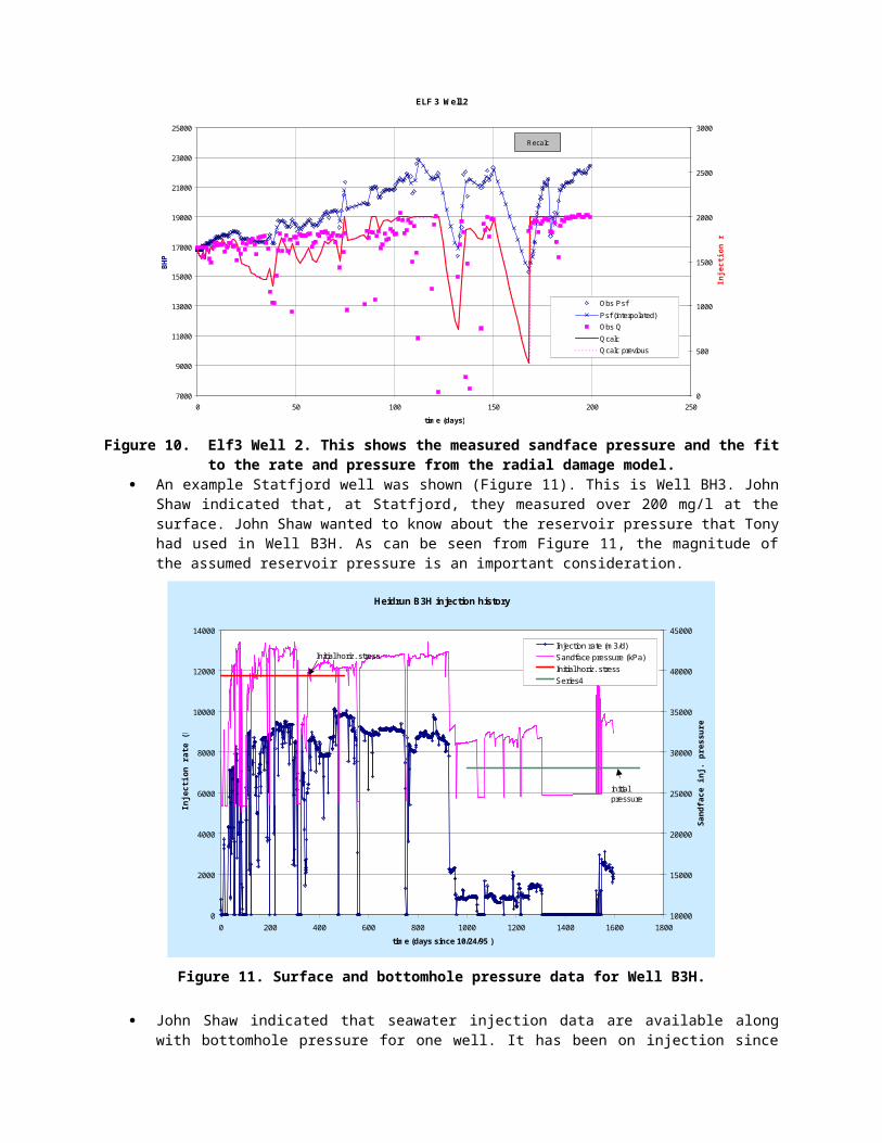
Tony Settari then showed Elf3 data. The radial damage model (described earlier was used to fit these data). These data were presented earlier (at the meeting in Amsterdam in September). One of the issues emphasized by John Shaw and others was that Tony might have added the high scale content to the solids used in the evaluations. Figure 10 is an example of these data.

ELF 3 Well 2

7000

9000

11000

13000

15000

17000

19000

21000

23000

25000

0 50 100 150 200 250

time (days)

BHP

0

500

1000

1500

2000

2500

3000

Inje

ctio

n ra

te

Obs Psf

Psf (interpolated)Obs Q

QcalcQcalc previous

Recalc

Figure 10. Elf3 Well 2. This shows the measured sandface pressure and the fit to the rate and pressure from the radial damage model.

An example Statfjord well was shown (Figure 11). This is Well BH3. John Shaw indicated that, at Statfjord, they measured over 200 mg/l at the surface. John Shaw wanted to know about the reservoir pressure that Tony had used in Well B3H. As can be seen from Figure 11, the magnitude of the assumed reservoir pressure is an important consideration.

Heidrun B3H injection history

0

2000

4000

6000

8000

10000

12000

14000

0 200 400 600 800 1000 1200 1400 1600 1800

time (days since 10/24/95 )

Inje

ctio

n ra

te (M

3/d)

10000

15000

20000

25000

30000

35000

40000

45000

Sand

face

inj.

pres

sure

(kPa

)

Injection rate (m3/d)Sandface pressure (kPa)Initial horiz. stressSeries4

Initial horiz. stress

initial pressure

Figure 11. Surface and bottomhole pressure data for Well B3H.

John Shaw indicated that seawater injection data are available along with bottomhole pressure for one well. It has been on injection since June. John will provide data. The value of this information will be for substantiating bottomhole pressure prediction tools and for evaluating performance with complete and reliable data.

Tony Settari had analyzed some of the presented data with the radial damage model. Henrik Ohrt suggested that you could use a radial model, after fracturing, below closure. Tony suggested that the permeability was large enough that it may not be an issue in this particular well.

Tony Settari then showed Marathon data. One of the relevant issues brought up was the specific completion method. It was indicated that Excluder screens had been used - 110 micron Excluder. It was anticipated that most of the pressure drop encountered is across the screens and that there are significant difficulties in cleaning these screens. This brought up the perennial stimulation planning requirement of identifying where the skin is coming from before pumping a remedial treatment. Some reanalysis of the Marathon data may be appropriate recognizing the contribution to the skin from the screens themselves.

IMPORTANT ADDENDUM: Bruce McIninch clarified misconceptions. “…Marathon did some test of pressure drop across sand screens while evaluating options for our North Sea West Brae development. The results are significantly better than presented in the summary of the Houston meeting. We took a range 3 joint of 6-5/8” 20 ppf tubing, drilled out perforations across the center 16’ and installed a single 16.5’ 20 micron Excluder screen cartridge with 0.012 gauge wire wrap and outer shroud. After pumping through lines and getting base pressures, we then did a multiple of injection rate tests through the screen. All pressure data were collected on quartz gauges. Included below are results.”

Rate(BPM)

5 10 15 18

Rate(BPD)

7,200 14,400 21,600 25,920

PressureDifferential

(psi)

0.5 3.7 12.4 24.4

DifferentialPressure

per BPD/ft screen

0.0011 0.0042 0.0095 0.0155

“The only limitation of the test was the pump. The 26,000 bpd rate was hardly fast enough to get water out of the top of the screen. We were happy with the results and utilized the product.”

“Other Comment: Would recommend KISS charges for injection not deep penetrators to reduce collapse damage in tunnel as you note. KISS charges are designed as big hole and no penetration. Only penetrate casing and cement with very minimal formation contact. Contact Phil Snyder Marathon Houston for study.”

NEED TO IDENTIFY WHERE THE SKIN IS OCCURRING. During wrap up discussion, it was indicated that Petrobras has a significant amount of

relevant information on the mechanics of plugging. Antonio Luiz Serra de Souza has provided two references from the Rio Oil and Gas Expo and Conference, October 16-19, 2000 – hosted by IBP [Brazilian Petroleum Institute] and held in Rio de Janeiro, Brazil. These are:

Bedrikovetsky, P., Marchesin, D., Shecaira, F.S., Souza, A.L.S., Milanez, P.V., and Rezende, E.: "Injectivity Decline Caused by Injection of Sea/Produced Water: Applications to Waterflood Management," IBP43300.

Serra De Souza, A.L.: Reservoir Management Directions for Reinjection and Disposal of Produced Water," IBP32600

Tuesday December 12, 2000

Discussion focused on horizontal injectors. There was an initial discussion period where horizontal injectors were "defined." For practical purposes" one definition was that a horizontal injector could be taken as anything that could not be reached by wireline, and/or that the horizontal/high angle component needed to be through or across the target injection zone(s).

John Shaw first showed a well on Gulfaks. It had been drilled in one fairly tight zone of the Rannoch. In a vertical well, the water just overrides into the high permeability Ness.

This horizontal has 425 m of perforated interval. They started injecting below frac pressure at 840 m3/day. This was considered to be a satisfactory but.... Field personnel were eventually "forced" to fracture this well because they lost another injector. To overcome this, they increased the rate and the PLT showed that the injected fluid dominantly went into one zone.

On the next well, recognizing that, without some control on injection schedules, fracturing would likely be concentrated in one zone, low rate injection was undertaken to precondition the well with cooling. This injector was in the Cook formation - drilled in the low permeability Cook 3. The pressure was gradually brought up - hoping to fracture along the length. There were about 450 m? of perforations. Despite these procedures, it was found that flow was concentrated only into the central part of the perforations.

Laurence Murray suggested that coverage could be improved by pumping in below - but close to - frac pressure and later increasing the pressure, as was done in John’s example well. But, if you take the pressure up too fast, the well will still frac preferentially in only one place. Laurence suggested that 840 m3/day, along a long well, was probably still inadequate for substantial cooling.

With improved drilling technology, some horizontal or ERD wells are so long that the temperature difference can be so large that the stresses are substantially different and you will only get fracturing occurring in one place. So how do you get the toe of the well started up (for example)?

THE SOLUTION ADOPTED BY MAERSK HAS BEEN DOWNHOLE CHOKES.

The operators were then canvassed as to who has horizontal injectors. Statoil has a couple on the Siri field. John Shaw emphasized that they found stable

injection in some of these wells. Siri data are available. Conoco has none. Bill Landrum felt that the non-fractured zones would go to zero

because of plugging. Petrobras has two or three horizontal injectors. These are soft formations and the

injected fluid is seawater. Antonio is uncertain of the completion specifics. Chevron has acquired some in Argentina. It was indicated that Shell might have a number of horizontal SWI wells in the North

Sea, single and multizone, various fields. Sponsors requested if Alastair Simpson

could find out if this was accurate and whether the information/learnings could be provided to the JIP.

Phillips - Carl Montgomery was not specifically aware of any although there may be some new ones just brought on line in Alaska

Norsk Hydro is looking to drill them on Brage. Laurence Murray presented on some of the BP Amoco horizontal injectors and

outlined the considerations for optimizing injection conformance. Laurence pointed out that some of the key considerations are: Well Trajectory Perforation Strategy Well Cleanup Injection Startup Well Performance Surveillance and Intervention Control

Laurence showed a slide of one situation in Prudhoe Bay. This is for a dipping reservoir - as you go south down to the periphery, there is a tar mat (immobile oil) and there is a very thin reservoir. The maximum horizontal stress in the area shown was determined, from breakouts, to be NNW-SSE. The injectors were put into Zone 4, above the tar mat, and there was variable reservoir quality. The original well was sidetracked and was about 85° through the top of the Ivishak. Temperature was used for the stress barrier. Seawater cooling occurred but the tar mat took about three years to cool and sense reduced stress. However, when switching from seawater to produced water, if you are injecting in the oil leg, you may eventually have a problem with stress barriers. Produced water injection would heat the previously cooled zone near the well but the remnant cooler zone farther away would temporarily maintain lower stresses and any induced fracture would want to grow downward into the lower stressed zone. The message is that cooling and heating will influence in-situ stress conditions and that to forecast fracture growth, the complete thermal history must be accounted for.

What do you do to control the injection profile?

1. Well Trajectory: Laurence discussed injection into some long horizontals. One well was drilled in the maximum stress direction and another was normal to this. They wanted to see if the performance was different for the two wells. Previous experience had suggested that tortuosity caused a significant loss in injectivity. Tortuosity is near-wellbore pressure drop that is caused by complicated fracturing characteristics near the well as fractures reorient to grow in a preferential stress direction. Presumably, near-wellbore pressure restrictions can be used to regulate the amount of fluid that enters specific intervals.

Conceptually, if you have a well that is poorly aligned - in inclination to the vertical and/or in angle to the maximum horizontal stress, theory and previous experience had suggested that there would be higher stress drops and these zones would take relatively smaller amounts of fluid. Consequently, consider drilling a "wiggly" well – parts of it may have more tortuosity than others – the conventional analog is limited entry stimulation where perforation density is used to regulate the amount of fluid going into particular zones by regulating pressure drop.Joe Hagen asked for clarification on the growth of fractures initiated in unfavorable zones – when, whether and how these will reorient themselves. Laurence indicated that the radius of curvature is a function of viscosity and rate. In an injector, this product is usually smaller than for a stimulation treatment and the radius curvature is smaller [they

will reorient more quickly]. In addition, the width is not maintained by proppant and shear stress effects could be significant.

Tony Settari believes that another difference in performance can be due to lower permeability in the well that was aligned with the stress field because of permeability anisotropy.

2. Perforation Strategy: An example perforation strategy may be that if the well is poorly oriented you may only perforate a restricted length. MINIMIZE cost. It was indicated that for horizontals that the perforating strategy was critical.

An example was given from a North Sea reservoir. Initially it was thought that there was only one contiguous sand along the horizontal extent, on the basis of initial RFTs. It was subsequently found that there were significant pressure differences across thin shales. It was essential not to blanket perforate in order to leave room to set a plug. In this well, they couldn't squeeze the water leg because it would all go into the oil leg.

3. Well Cleanup: Make sure that the perforations are clean. Laurence showed an example from another reservoir where there was and was not a backflow through the perforations. Conformance was superior in the situation where the perforations were cleaned by backflowing. Caution - This is hard rock.

In one of these wells they used different perforation densities to act as a choke and control inflow. Cleaning perforations can be accomplished by shooting underbalanced or by backflowing. In one case, they had to lift water. The length of the interval was about 450 feet at maybe 20,000 ft MD. They also brought the well on slowly.

Laurence suggested a criterion for backflowing of five gallons per perforation – presumably this is well/formation-dependent to some extent. Make sure that the well is lifted enough to try and clean everything out. Concerns were raised about handling returns in some cases. This can be a particular problem with floaters – backflowing may not be an option.

Charge type? Use deep penetrating charges in moderately hard rock and some of the weaker formations to try and get beyond damage.

4. Well Performance: As has been indicated, thermal preconditioning can be a possible means for controlling conformance. During cooldown phases, it is important not to cause substantial plugging along the well during low rate injection. Otherwise, it will not be possible to cool the entire well. Thermal pre-conditioning can be quite valuable.

Laurence showed another example where they didn't want to abandon the lower zone. The upper zone had variable reservoir quality with permeabilities from 10 to 100 md. The lower zone had lower stresses and was maybe cleaner. If injection were carried out initially without isolation, the lower zone would have taken the bulk of the fluid because the stresses were lower. To overcome this, when the injector was first put on line, they put an RBP between the upper and lower zones, fraced the upper zone and pumped reasonably clean PW into the upper zone. The heavier and hotter produced water entered the upper zone and because of the temperature the bridge plug didn't contract. They pumped produced water for a couple of days and then switched to cooler seawater. The bridge plug cooled, shrank and unseated. Fluid would now also enter the lower zone but the pre-fracturing in the higher stressed upper zone improved flow distribution. Note that this well had been intended to be a seawater injector - this was why it was not kept on produced water injection. This concept has been used the other way around in soft rock, West of Shetlands.

Laurence gave another example of mechanical isolation methods. This was for a high angle well, approximately 1.5 km long, completed with wire wrapped screens. They set

ECPs at the toe. Laurence cautioned that more than 50% of ECPs set in openhole fail. After setting two ECPs, while the washpipe was in the hole, they fraced the toe of the well through the washpipe - in order to get at least some flow through the toe. This type of pre-stimulation is more difficult in soft rock because you may not have substantial temperature effects. As a consequence, you may be able to thermally frac the heel and hydraulically fracture the toe - or vice versa.

5. Hydraulic fracturing for profile control: BP Amoco has found that the proppant gives a temporary benefit – the injectivity goes back to low levels after 12 to 18 months. The reason is basically plugging because there is poor communication. There are only a small number of perforations open to the fracture and this entry is easy to damage. Laurence has found that the same thing happens with seawater [be careful – this is an issue of the area of entry into a fracture orthogonal or at least cutting the well at an angle – the open area is small and conducive to plugging – in other instances, where entry is not such an issue, seawater has been used for remedial cleaning of fractures damaged by produced water].

Laurence indicated that you might be able to get a benefit in some areas where you cannot get any injection in otherwise [i.e., use a propped fracture].

Frac packing may be better solution to the filtration problem at the well/fracture junction. You may have better contact at the wellbore.

Propped hydraulic fracturing may have better application in gas injection than in water injection - provided that the gas is clean.

BP Amoco would always select unpropped fracturing if they possibly could. Laurence indicated that it is possible to approximate critical injection rates for out of

zone growth using a radial fracture model that is not growing - with the fluid loss moderated by the PEA-23 relationship.

Laurence described startup of a high angle injector in Prudhoe Bay. They pumped at a constant rate, cooled the well (or at least some of it) and the frac gradient consequently dropped. If the rate of injection is appropriately low, the fracture stays behind the thermal front. After stabilization, increase the pressure back up to the original pressure and try to cool and open other zones. They completed a 1000 ft section with three discrete 100-foot perforated zones about 100 feet apart. Techniques such as these allow you to use thermal effects to control the fractures. This well was started up at two rates. kv is slightly higher farther down in the section. They found a slightly better flow rate at the toe although the split in flow was fairly good. Laurence believes that any of the cooldown techniques become more difficult in small diameter pipe where it is harder to get the rates that are required for widespread and acceptable cool down.

Alastair Simpson provided a word of warning. He is familiar with a situation where the cooldown process had been ongoing but the well was shut down. Warmup occurred and the operator had to go through the whole process again. This was supported by Laurence Murray who also emphasized that BHT cannot be treated as a single number in ERD/HA wells. He showed a temperature profile for one situation where the change in stress due to thermal effects would be somewhere in the neighborhood of 15 psi/°F. For good conformance there is a minimum flow rate for cooling. You need to look at friction effects and there is probably a maximum flow rate. There is a window of operation for these wells.

Along these same lines, a Hall plot was shown for one well. The Hall plot did not show a problem. Offset wells showed good performance. But the temperature survey and warmback profiles were instructive. There were seven intervals and all of the flow was in one interval. Maybe interpretation of the PLT was actually a problem. This well actually curves and the warmback shows a fracture running along the side of the well. Warmback showed this happening.

6. Monitoring, Surveillance and Intervention Control. This requirement was strongly emphasized, including new generation methods (fiber optics) and conventional techniques such as PLTs. The real costs of conventional PLTs were emphasized including deferred (or lost) production. BP Amoco are now using downhole sensors and fiber optics. You can use these themselves for PLT evaluations without intervention. MUST ADD FIBER OPTICS TO MONITORING SECTION - The frequency of back scatter

indicates the temperature. Fiber optics equipment can be run permanently or pumped in or out. The manufacturers are improving the equipment for measuring pressure.

In addition to continuous monitoring, the premise behind these measurements is that you can be misled if you exclusively use surface measurements. An example was given. A constant slope Hall plot was derived – from surface – or for that matter bottomhole pressure. Even though the Hall plot was constant, a bottomhole survey found that going from seawater to produced water had changed the conformance. Distribution of the flow was different. Flow was going into a residual frac. They have backed the rate off so that they are now injecting into partially closed fracture.

If you are going to do surveillance you need to be able to do something about it. There is a need for flow control.

Tony Settari next did a review of various methods that can be used for analysis of horizontal wells. This presentation is available. There was an important message:

Available analytical methods will fall short more quickly than for vertical wells.

Tony outlined techniques for unfractured horizontals. There are analytical methods. Normally there is no plugging included. Tony showed data from Kuppe and Settari, 1998. These simulations showed that the models from Goode and Kuchuk, or Babu and Odeh may give the best answers and that Joshi's method is the worst. The Babu and Odeh technique generally underpredicts the injectivity index - but this may be preferable.

Numerical modeling can be carried out but reservoir heterogeneity is still difficult to deal with. If there is permeability damage, Tony doesn't see any legitimate available model.

In addition to reservoir issues, wellbore hydraulics and thermal effects can have overwhelming effects. The analytical models will have a hard time handling time-dependent effects.

Is there a middle ground for the level of modeling – so that expensive, time-intensive numerical simulations are not required?

Tony also discussed fractured horizontal wells, considering static and dynamic (growing) fracture situations.For static fractures – fractures that have been propped or acidized and where there is clean water injection, there are some possibilities for representing well performance. These include methods by:

Karcher. Mukherjee and Economides. Tony warned against using the method published by

Mukherjee and Economides. This model is based on a straight-line relationship between PI and a dimensionless fracture half-length, xf. It does not include spherical flow and this consideration makes the prediction worse as the permeability becomes higher.

Levitan.

Assorted Norwegian work. Kuppe and Settari. Kuppe’s method assesses the contribution from single, transverse

[normal to the wellbore], fully penetrating [covers the entire reservoir height], static fractures. The analyses show that there is a very large gain for adding a small fracture – This EMPHASIZES THAT THERE IS NOT a SUBSTATNTIAL GAIN FOR LONG FRACTURES.

Correlations have been developed for multiple, static fractures. It is in the form of an Excel spreadsheet. The number of fractures has to be odd, but this should not be a real issue. These correlations, based on numerical modeling, incorporate kv/kh, and height.

The equations and spreadsheet could be made available. This is for static fractures.

Anything more complicated than this and you need to go to numerical simulation. One of the difficulties in such numerical simulation is the method for putting in the fractures. It results in very slow runs in Eclipse, for example, because of the fracture. There are specific PWRI issues – stress-dependent fracture conductivity for thermal and pore pressure effects needs to be considered. Even though you are in liquid flow, turbulence may be a factor. If you are considering reopening, the simulation may be very difficult.

Carl Montgomery wanted to know if interference between fractures was included in the spreadsheet that was mentioned. Tony Settari indicated that it would be represented in a simulator. Tony indicated that there is numerical technology for multiple static fractures but it is difficult and expensive. Tony indicated that, in the past, he has simulated this for a very heterogeneous, compartmentalized reservoir with multiple fractures (static). This type of modeling is expensive and time-consuming and the spreadsheet alone may be valuable for indicating relative differences between different completion strategies.

For dynamic fractures – continuing growth or recession of one or more fractures during injection - some of the relevant questions and issues were:

1. Where do they start? 2. What sort of competition will exist between the fractures? 3. Conventional models can be used if you take into account the additional effects of

wellbore hydraulics and the entrance geometry can be modified. Ahmed Abou-Sayed believes that this is true but he is concerned about representing the hydraulics.

4. Tony talked about competition between multiple fractures. Sirivardane, 1994, coupled a wellbore hydraulics model with multiple hydraulic fractures using a conventional hydraulic fracturing growth model. The results were biased by the assumption of a KGD fracture geometry. This is similar to what Laurence Murray has done in his multilayered spreadsheet model - he has coupled a simple model with the hydraulics. Strictly speaking you may need a more realistic model for the fracture growth. Tony emphasized that an accurate model of net pressure in the fracture is essential – he showed an example... Henrik Ohrt asked why this would not be included in the Toolbox. At a minimum, Henrik wanted the small-scale fracture interaction studies like Tony's Excel spreadsheet.

5. Ahmed said that, from the work that Advantek has been doing on the data from Maersk A and B, wellbore hydraulics is dominant.

6. TONY COMMITTED TO PROVIDE HIS EXCEL SPREADSHEET FOR MULTIPLE STATIC FRACTURES.

7. Tony also talked about the influence of turbulence. Convergence/divergence effects becomes significant for horizontal wells. Turbulence can reduce the benefit of

fractures at high rates! On the other hand, the near-wellbore entrance pressure effects due to turbulence can be used to your benefit – it may allow you to create additional fractures!

8. Finally, Tony indicated that there can be significant partial penetration effects.

There followed some basic discussion of simulations on a horizontal injector in Alaska, using BPOPE and using V.I.P.S.

1. BPOPE calculates geometry at discrete periods. It does iterate and ultimately checks to ensure that there is convergence between the fracture pressure and any sort of poro-thermoelastic stress field modification. There is computational overhead in going back to see if there has been adequate convergence.

2. The V.I.P.S. runs showed that there are joints opening but the code never reached fracture pressure. There was never any matrix flow in V.I.P.S. The V.I.P.S. simulations apparently did not adequately represent the situation, partially because, even though the reservoir would be cooled down by seawater injection, the PVT data did not change with temperature. Tony indicated that there were other modeling issues. He found that the frequency of updating in GEOSIM was important.

3. A practical observation from the simulations was that Tony found that, operationally, you might need to spend a SIGNIFICANT amount of time to pre-condition the well.

At this point, discussion focused on what needs to be done to provide an appropriate product for Task 6 on Horizontal Injectors. The consensus was:

1. Provide Best Operational Practices and particularly indicate some of the conformance control options that may be available. This needs to include methods for surveillance and flow control.

2. Provide Best Modeling Practices - How to simulate and how not to simulate. 3. Provide certain basic tools. This would include the multiplayer/multilateral

spreadsheet model that has been provided by Laurence Murray and the Excel correlations that Tony has developed for multiple static fractures.

At this point, Ahmed Abou-Sayed spoke on PWRI Knowledge Management, including the Economics Model and the Toolbox.

Ahmed first provided an Overview of Toolbox, including:1. INPUT DATA 2. PERFROMANCE METRICS 3. HISTORICAL PLOTS 4. WATER SOURCE

Carl Montgomery is concerned about over-specifying the type of treatment to be called out. Everyone agreed that this was an issue. One of the components of the toolbox would provide general guidelines on effective treatment types. It was agreed that the toolbox would not supply specific levels of information on treatment chemicals etc. There may be generic observations on compatibility, acid concentrations, etc., but nothing more specific. Other specific observations/requests for change included:

Put in another button - DIAGNOSTICS The Toolbox needs a specific tie in to the Best Practices Provide a keyword search.

Provide a dropdown box that interacts with the spreadsheet. Be certain that units’ issues are resolved. Need to show the units on the input form. Be certain about date merging. Resolve issues of converting ASCII to Excel format. Fix well name to be imported. Provide a splash page to include the assumptions and warnings!

After presenting the Toolbox there was a presentation on the Economics module. There was a tremendous amount of controversy and diverse interests in what was desired. Some of the comments made (non-prioritized) are indicated below.

Laurence Murray asked if the Best Practices could be used to assist in the ranking of the most appropriate stimulation treatment. How do you risk the selected options - Performance Metrics are provided?

Can you map the Best Practices against the risk factors with a User Override? You would at least have the risk field present for the user to input. It would be a technical risk factor - use it or not.

Maybe some information can be gleaned from the Best Practices. How do you enter risk beyond this? Henrik Ohrt wants to keep it simple.

Distribute the equipment database to the Sponsors "for a reality-check." Carl Montgomery indicated that the facilities department may do a lot of the

comparisons and pricing that was proposed. Using the database may be an option but it might be more appropriate to just input a single number. Carl thought that the proposed worksheet might be too ambitious. Henrik Ohrt felt that it should be used with great caution.

Carl Montgomery brought up the opportunities that may be provided by Halliburton's SurgiFrac service.

The installation cost does not necessarily depend on the capital cost. One suggestion was to have an Installation Cost Button in the CAPEX.

Discussion continued for some time, after which there was a closed-door Sponsor’s Meeting.

Wednesday December 13, 2000

Quan Guo provided an update on the data analysis that Advantek has been undertaking for Task 2 (Matrix Injection) and Task 4 (Stimulation). This presentation is available. Some of the observations/contributions included.

1. To date, some form of evaluation has been performed on 145 wells (30 in chalk, 8 carbonate wells, and 107 sandstone wells). The reported permeability for these wells ranges from approximately 1 md to 10 darcies. Of these wells, approximately 40 have oil-in-water and TSS data. One plot, shown in Figure 12, was somewhat controversial. It is for a Statoil field. In the September 2000 meeting in Amsterdam, when John Shaw had presented this data case, he had suggested no strong relationship between OIW and injectivity. Figure 12 suggests that maybe there is some relationship after all. However, all of these figures have to be reviewed with caution in case there are other complimentary changes in operations or fluid (e.g., temperature changes, etc. going on at the same time). In Figure 12, the pink curve is a PEA-23 type relationship where the constants used with the OIW and TSS in the PEA-23 relationship were modified to get a best fit to the data. This seems to suggest that the functional form of the PEA-23 relationship is applicable. The permeability of this reservoir is about 120 md, not too

dissimilar from some of the Prudhoe Bay data used in developing the PEA-23 correlation. CAUTION – ADDITIONAL WORK IS REQUIRED TO BASE CALCULATIONS ON BHP RATHER THAN WHP.

Water Quality

0.00

2.00

4.00

6.00

0 500 1000 1500 2000

OIW

IIII II Calc

Figure 12. Plot of injectivity index versus OIW for one Statoil well with a superimposed PEA-23 type relationship.

Comparisons were made between produced water and seawater injection data. There were no real surprises here. Examples were shown for two Maersk wells (see for example Figure 13) and for BP Amoco. The behavior can be at least conceptually rationalized by accounting for thermal and poroelastic stress modifications. The superior performance of seawater was not as evident in non-Prudhoe Bay, suggesting the role of complimentary injection parameters, fracturing, viscosity changes, etc.

Injection Periods

010

0020

0030

00

0 2000 4000 6000 8000 10000 12000Injection Rate (BPD)

WH

P (p

si)

SW 3/27/93-3/3/97 PW 3/3/97-5/1/97 SW 5/1/97-4/12/98 PW 4/12/98-8/4/99

Figure 13. Wellhead pressure vs. injection rate for Well B-01, in chalk with a permeability of 2 md in an injection zone with a thickness of 277 feet.

Injection Performance A-03

050

010

0015

0020

00

0 5000 10000 15000 20000 25000 30000Injection rate (BPD)

Wel

lhea

d Pr

essu

re (p

si)

SW 1 PW1 SW 2

Figure 14. Wellhead pressure versus injection rate for a Prudhoe Bay Well, in sandstone with a permeability of 200 md in an injection zone with a thickness of 224 feet and a porosity 0f 25%.

2. Some data were also presented for blended injection – e.g. specific mixtures of seawater, produced water and aquifer water. Again, there were no real surprises in terms of the relative relationships between the curves. Norsk Hydro data were shown. It was argued that blending aquifer water with produced water seemed to improve performance (this has not been strongly supported). One can imagine that this observation may be the case because of temperature, quality [note that aquifer water may not always be clean] and bacterial levels, etc.

3. Evaluation of some Prudhoe Bay data suggested that brief periods of gas injection between produced water injections seem to maintain good injectivity (Success of WAG). This should be treated as an observation rather than a conclusion. One well shown is a Norsk Hydro well; a sandstone with a permeability of 100 md and a zone thickness of approximately 130 feet. Figures 15 and 16 illustrate performance. The precise methodology for calculating a gas equivalent rate was not specified. In the database, there is also a substantial amount of Prudhoe Bay data where miscible injection was carried out.

Injectivity History

010

2030

40

15-Jun-94 28-Oct-95 11-Mar-97 24-Jul-98 6-Dec-99

Date

II (B

PD/p

si)

00.002

0.0040.006

0.008

G II (BPD

/psi)

Injectivity Index Gas II

Figure 15. Injectivity. Ignoring the calculated values for gas injectivity because of uncertainty in terms of how it was calculated, liquid injectivity does increase following gas injection – whether due to relative permeability, temperature, sweeping away damage or whatever.

Injection History

015

000

3000

045

000

20-Jul-95 15-May-96 11-Mar-97 5-Jan-98 1-Nov-98

Date

Inje

ctio

n R

ate

&

WH

P0

24

68

10

Gas Injection R

ate

Injection Rate WHP WHP Gas Gas Injection

Figure 16. Parameters during water and gas injection.

4. Some examples were provided showing the influence in temperature – either for changing the thermal stress regime or for changing fluid viscosity. No surprises - but the data can be important for quantifying thermal stress effects.

5. Data were shown that indicated decline in injectivity as a function of particle count and size, but apparently more a function of count than size. Advantek suggests that the

effect of TSSW is better related to particle count (ppm) than to mass concentration (mg/l). Examples were provided from Statoil and Elf (Figures 17 through 20).

II vs. TSSW

01

23

45

0 2 4 6 8 10 12

TSSW (mg/l)

II

Figure 17. Variation of injectivity index with the total suspended solids in a Statoil well, in sandstone, with a permeability of 120 md and a zone thickness of 37 feet.

II vs. OIW

01

23

45

0 100 200 300 400

OIW (mg/l)

II

Figure 18. Variation of injectivity index with the oil in water in a Statoil well, in sandstone, with a permeability of 120 md and a zone thickness of 37 feet.

II vs WQ

01

23

45

1 2 3 4 5 6 7WQ

II

II Calculated II

Figure 19. This is a crossplot of the injectivity index versus what appears to be the total suspended solids water in a Statoil well, in sandstone, with a permeability of 120 md and a zone thickness of 37 feet. The superimposed curve is a modified PEA-23 relationship.

Water Quality

01

23

45

0 500 1000 1500 2000

OIW

II

II II Calc

Figure 20. This is a crossplot of the injectivity index versus the oil in water for Well Elf-2 in the field Elf-2. It is a carbonate with a nominal porosity of 20%, a reported permeability of 3 md and a zone thickness of 194 feet. The pink curve is a best-fit application of the PEA-23 relation using different constants. The deviation in the 600 to 1100 ppm range emphasizes that other parameters must be concurrently included.

6. A new correlation may quantify the influence of filtration, based on particle count and size. This correlation needs verification with additional field information (already available to the JIP) and this effort will continue. Most of the damage is caused by smaller particles (5m) yet these particles have a deceptively small combined mass. Most of these conclusions were derived from an evaluation of the Maersk B field. Particle size information was available and injection rate was plotted against particle count for different particle sizes. Apparently injection pressure was not considered.

7. Observations suggested a potentially revised version of the PEA-23 correlation for use with matrix injection and possibly for fractured injection for reservoirs with permeability outside of the PEA-23 range. No comments were made on temporal variation. Bill Landrum asked whether there was any obvious dependence on particle deformability. John McLennan indicated that that data might not be available in the information that Advantek had to evaluate. Joe Hagen felt that this would be important. Laurence Murray indicated that when he had done it in PEA-23 that he had explicitly gotten away from this because there was too much scatter in the data - Quan's proposed route would require additional measurements.In terms of particulate compressibility, the question was asked, "How do you measure oil and solids in the same fluid?" Paul Jones indicated that it was difficult to determine what was oil and what was a solid even in oil and that it would be difficult. Laurence Murray suggested having on-line measurements – BP Amoco does on Harding. Paul said they do this as well, but he still remains concerned about the detection capabilities. Quan proceeded on and discussed some of the observations that they had made on effectiveness of stimulation, largely based on evaluation of Maersk data. These included the following. Improvement due to stimulation returns the well to the average best historical

injectivity index (you cannot do better than the previous best). This would seem to be an important observation. You might ask whether this is applicable to higher permeability reservoirs and whether or not removal of completion damage, particularly for matrix situations, will not obviate this conclusion.

When you do acid treatment are you really removing the damage? This could be an important conclusion. Is there adequate diversion, are large enough treatments pumped, has the treatment been performed too late in the injector’s life?

Delayed, gelled, buffered and/or chelated acids will do better than normal acids. Presumably this is an observation from other Advantek experience and basic logic suggested that acid spending should occur deep enough into the formation. Laurence Murray supported the potential use of delayed, gelled, buffered and/or chelated acids - plus appropriate diversion. In essence, these are just good acidizing practices.

From the evaluations to date, Advantek highly recommends stimulating an injector early in its life, if not before it is brought on line. Presuming the conclusion that injectivity cannot be better than initial levels, this conclusion is logical.

The data suggests that timely stimulation is important. An example of good stimulation timing was provided where the decline was caught early. It was argued that there would be a severe decline in injectivity, leading to damage that would be pseudo-permanent if treatment is delayed for too long.

Some of the Maersk wells were treated by bullheading acid while acid was metered into other wells at concentrations of 1.5 to 2%. (Advantek was reminded that metering methods were in error because of orifice scaling.) The Maersk treatments suggested, as might be anticipated, that 15% HCl was effective. The jury is still out as to whether metering in lower concentrations was more or less effective than using 15%. It did seem that the Improvement Ratio (a parameter characterizing the effectiveness of the treatment) was larger when the treatments were bullheaded. The injection rate remains constant for a long period of time after the stimulation. It is

uncertain whether the same conclusions can be drawn for sandstone reservoirs. It would be expected that this might not be the case and that alternate formulations would be required. The question is "What does the acid really remove?"

An important contribution of the recent Advantek work is the definition of an improvement index, and a parameter called the DRII, allowing comparative evaluation of the success of stimulation operations.

According to various reports, an improvement was seen in performance due to the addition of the acetic acid (placement, delay, buffering). The Maersk database includes horizontal as well as deviated wells. The deviated wells were treated with HCl only, whereas the horizontals were treated with a blend of hydrochloric and acetic. "Acetic and formic acids are sometimes used as retarded acids. Also, they are used as mixtures with hydrochloric acid. These weakly ionized acids react at a much slower rate than hydrochloric acid, even at very high temperatures. However, they are less efficient in terms of their ability to dissolve carbonates since large amounts of unspent acid remain after reacting for long periods of time. … An additional disadvantage is their increased expense. …. However, they do offer certain advantages in some treating applications. Being naturally less corrosive, they can be inhibited at high temperatures for long periods of time. This has led to their use as perforating fluids." [1]

Performance was evaluated using a trailing average injectivity index. The reciprocal injectivity index (RII) in the Maersk wells after acid stimulation seems

to average about 70% of its trailing RII average. 8. Quan Guo showed plots derived from the Toolbox and indicated that you can go to the

database and find analogs. 9. Alastair pointed out that upset conditions someone needs to be considered. Bill Landrum

supported this. Conoco's findings are that it is the episodic effects that cause real injectivity degradation problem. Laurence Murray indicated that it is probably the solids causing the problem. Bill Landrum argued that oil might affect the relative permeability. Laurence Murray countered that he felt that it depended on whether you were injecting into the oil or the water leg

10. Henrik Ohrt suggested that it would be worthwhile to generate chronological discrimination; that is, in addition to showing all of the data, show data in different colors or symbols for different periods of time and operational events – as was done earlier in the project for some Shell data.

11. Jean-Louis Detienne brought up the necessity for discriminating between thermal fracturing and "regular," hydraulically induced fracturing.

12. Jean-Louis emphasized the importance of correctly calculating injectivity indices for situations where fracturing has occurred. The PEA-23 correlation correctly takes into account the changes in slope after fracturing has occurred. It is essential to standardize comparisons of data to guarantee the same interpretation of II. He emphasized, as was done in PEA-23, the need to correct slopes for temperature and viscosity to sort out the effects of water quality. Jean-Louis insists that all contractors must use the same methodology.

13. The observations so far are that the evaluated data has the same functional form and incorporates similar parameters to the PEA-23 correlation but that particle count may be more important than mass.

14. Paul Jones stressed that the relationship should not use mass or particle count - that neither one is properly measurable. Chevron lumps their data because they cannot trust the particle count or mass. Chevron uses the water quality ratio.

15. Ahmed Abou-Sayed argued for adding pore throat dimensions. Laurence Murray argued that the PEA-23 relationship incorporates this.

16. Bill Landrum agreed to provide Conoco data from California and again emphasized the important deleterious effects of episodic upsets.

17. Laurence Murray asked if you needed acid at all. In propped fractured injectors, BP Amoco has found that seawater was as effective as pumping acid. On Forties - every three months – they flush with seawater. Laurence asked an important physico-chemical question – in sands what good is the acid by itself - if it is not attacking particles?

Summary of Operators Meeting Held on Tuesday, December 12, 2000

At this point, Laurence Murray gave an overview of what was discussed the previous afternoon at the operators meeting; including the key work priorities, the next meeting, what happens after July and "What do the Sponsors want to do with uncommitted money?" The items brought up included:

1. The Toolbox looks good but it needs to be polished up (and off). For example, put in units and make it "idiot proof" and have a warning indicating what the assumptions are and a warning on how to use it. The Sponsors want it on CD and not just on the web. Sponsors want a copy as soon as possible. Some Sponsors want the Toolbox, as is. All sponsors need a version by the end of January so that they can exercise it before the next meeting. There can also be a final beta release before the next meeting – Provide the Toolbox to Jean-Louis Detienne immediately, a version to all Sponsors by the end of January and the final beta release by March 15.

2. Coordination and tying together of Products. Be certain that links are correct; that data are in the right place, etc. and be certain that the Best Practices integrate seamlessly with the Toolbox. It is essential to have a way for going to and from the Best Practices. Contractors need to clarify how this will be done. The ToolBox needs to have a Diagnostics button clearly taking the user to where diagnostic calculations are done. In the version shown this was done by clicking on wellbore hydraulics, which is not a satisfactory delineation.

3. Proposal for Well Testing. Some time ago, it was suggested that there are gaps in technologies for well testing - what needs to be done? A proposal for that was requested – the Sponsors would like to see this as a part of the Toolbox. Clean it up and get it out. If a well testing part is done it should be part of toolbox.

4. Horizontal Wells. Based on the presentations earlier in the week, it was decided that the deliverables for this Task are 1) produce Best Practices guidelines covering design, operations, simulation and surveillance/data acquisition. Solids and oil content needs to be included. Horizontal wells needs to be ready by the end of the first quarter.

5. Well testing of horizontals.In addition to surveillance – should be included in the Best Practices. The spreadsheets for analytical methods described need to be included in the Toolbox.

6. Validation. There are a lot of potential field tests being implemented. It is important to develop a Field Trials Best Practices covering critical aspects of implementing and interpreting pilot testing - e.g. "What would have to be done in converting from SW to PW?" "If you are going to retrofit, what would you do differently on land or offshore?" "Can/how only one well be used?" Operator interview!!!!! Operators needed to be asked as to whether various tools have been used and have they worked? This needs to be tied down by the end of the first quarter.

7. The Sponsors requested an update from Advantek on what has been done with the HWU data? They believe that the issue has been addressed, but ...

8. In all of the field data analyses, make very clear what types of formation have been tested and where this is done?

9. The focus is to tidy up what is available before the next meeting. For that meeting, AGIP has asked to host the next meeting. Tuesday March 27 through midday on Friday March 30, 2001 was proposed. If these dates need to move - make it the week earlier rather than the week later. Contractors were reminded that there needs to be a beta release at least of the ToolBox/Best Practices one to two weeks before the meeting.

10. A final issue is that there was not really a quorum of operators present - need to get approval.

11. Discussion then came down to the Economics Model. The Sponsors are concerned that it is going to divert resources. They felt that the principle is good but that the detail is extreme. "Who is going to use this and what is it going to be used for?" The Sponsors present believed that the level of detail is beyond what they want. They believe that it needs to be reduced to a manageable level. For example, there need to be major cost categories. The module must INCLUDE CAPEX installation costs. There needs to be a way for putting in the potential benefit - some sort of production information. Regional information needs to be put in as a default. The Ferguson paper provides some geographical costs. Use gross regional numbers – the Sponsors want the entries to be at the "gross" level - major categories plus regional information. It was acknowledged that it requires a lot of work to come up with geographical costs. The Sponsors also want to know about the various cost environments - land versus offshore. There is a need to know overall system costs to establish what is the incremental benefit. The idea is to have a screening tool at a very high level and someone else would do the detailed economics. The bottom line was that the Sponsors want something manageable. Propose what will be done at the next meeting - Don't Work On It - propose what the final product would be. The Sponsors said that they would need to look at the flow chart that was proposed for the Economic Model again. Defer a funding decision until the next meeting. Don't divert effort.

12. A major issue was what to do after June. The Sponsors felt that they would want some kind of ongoing maintenance. They would like to keep a web presence and ToolBox maintenance - e.g., might add well testing to the ToolBox or add or change tools. The Sponsors will need a quote for the website maintenance. They did not think that it would be substantial. The Sponsors need a quote for maintenance of the ToolBox outlining the issues and costs of normal product maintenance considerations and who will be doing it? John Shaw added that there will be quite a bit of good quality data coming in - new data should be good quality – and the Sponsors would want a way to be able to capture these data and these new data may make a significant difference in terms of some of the conclusions that have been or will be drawn.

13. Laurence Murray indicated that the Sponsors don't want to lose the industry consortium and specific methodologies/products/ proposals etc. are necessary for keeping the group together.

14. What do the Sponsors want to do for the rest of the money? Most Sponsors have not budgeted for 2001 PWRI JIP participation. They want to use the remaining money. The Sponsors will want a proposal on the well testing piece. The Contractors can get a proposal together on development work - some fundamental science could be included as was identified at the Monitoring Workshop.

15. Although there continue to be disagreements, at least some of the Sponsors believe that they have an idea of what is happening during injection - e.g. where do the solids go - e.g. natural fracturing. All seemed to believe that there may not be one single simulator for representing injection phenomena in different environments. There are simulators that deal with individual pieces. The suggestion, while a consortium of operators is available, was to modify existing code (that is not a full blown reservoir simulator) and get some of the "understanding" incorporated into a uniform "industry-standard" simulator. It would be desirable to have a group of operators using a uniform package - which the operators can all agree with on a technical basis. The Sponsors need a proposal on how to get this "understanding" into a simulator. The one suggestion was to use standard numerical techniques such as near-well modeling, where there is local grid

refinement and integrate this into a conventional simulator. The near-wellbore module needs to be flexible enough to mate with different reservoir simulators.

16. There may be enough seed money that the near-wellbore module can be designed to be used with any standard commercial simulator. Another specified requirement is that this needs to be able to run standalone. The first step is feasibility. How come you use it to relate to recovery? You could get a reservoir engineer to use this - a module. Put it on paper was the message to the Contractors – and make some preliminary recommendations/ proposals about the architecture. Indicate the processes that need to be incorporated.

17. Allow the Sponsors to discuss the proposal. Acceptance will be made difficult because the operators might disagree. Provide conceptual ideas and present these to the operators. Indicate how IPR from the project can be used. There is the potential to bring in outside parties. The Sponsors want to have the proposal available and circulated before the next meeting. This will be a joint Contractor proposal.

18. An additional issue was "What can the Sponsors do with the IPR from this Project?" The Sponsors have requested insight from Bob Siegfried - i.e., can this IPR be sold or licensed and what are the individual Sponsors rights? Can this product be licensed to other people?

19. Laurence Murray indicated that it was essential to speak to the other participating operators about the use of the remaining money – including, for example, the well testing proposal, maintenance of what already is available - further development - this is included in the maintenance, updating the existing data if/as new information is available etc. There is money available for 2001. For 2002, there is no new money put in and the current participants want to leverage the existing and expended money.

After the Operators’ meeting was summarized for the Contractors, discussion went back to the flow chart on Economics Model that Ahmed Abou-Sayed had previously presented. Some of the points from the ensuing discussion are as follows.

Is the flowchart an acceptable concept or is it not? The operators want a cost per kilogram of facility - that level of difficulty – i.e.,

simplify the process substantially. You may have a cost database but the Sponsors want it to be much simpler?

You do not need the level of detail in the Economics Model but the level of detail might be required in the Surface Systems Tool.

Antonio - brought up about decline rates - global economics - recovery - put in a value of a bbl of water injected. Different qualities of water - different recoveries.

Above or below frac pressure Frequency of stimulation Interaction with water quality Injectors Startup/conversion costs – i.e., new well for PWRI, converted producer to PWRI,

change from seawater or aquifer water to produced water. Oil removal costs – specify Solids removal costs - specify

Ahmed gave a presentation on some work that Advantek has carried out for horizontal wells. The issues of importance included standoff from the oil/water contact was an important design consideration, and undulation of the well trajectory was an issue (Joe Hagen indicated that this has worked successfully [undulation] on certain producers in Alaska.) Advantek

found that undulating wells had an insignificant impact on the total injection volume but had a maximum impact on the recovery, partly by helping compaction drive to last longer.

There was discussion of the need for simpler tools to deal with horizontal injectors - a spreadsheet type tool for horizontals.

ISSUES ABOUT THE DATA. Jean-Louis Detienne is interested in the amount of data that are available for Tasks 2, 4 and 6. He wants an update on the amount of data that are available from the appropriate Contractors. This would need to be in the form of a Table, similar to what Tony Settari has done for Task 3 and would include Field, Rock Type, Permeability, Oil [], Water [], Fracture Type, II/IIo ...

Meeting Adjourned.

1. Crowe, C.W.: "Principals of Acid Fracturing," Reservoir Stimulation, M.J. Economides and K.G. Nolte (eds), Second Edition, Prentice Hall, Englewood Cliffs, New Jersey (1989).