Putting the Patient in Patient Reported Outcomes:

A Robust Methodology for Health Outcomes

Assessment

May 2014

Abstract

When analyzing many health-related quality-of-life (HRQoL) outcomes, statis-

tical inference is often based on the summary score formed by combining the

individual domains of the HRQoL profile into a single measure. Through a se-

ries of Monte Carlo simulations, this paper illustrates that reliance solely on the

summary score may lead to biased estimates of incremental effects, and I propose

a novel two-stage approach that allows for unbiased estimation of incremental

effects. The proposed methodology essentially reverses the order of the analy-

sis, from one of “aggregate, then estimate” to one of “estimate, then aggregate.”

Compared to relying solely on the summary score, the approach also offers a more

patient-centered interpretation of results by estimating regression coefficients and

incremental effects in each of the HRQoL domains, while still providing estimated

effects in terms of the overall summary score. I provide an application to the es-

timation of incremental effects of demographic and clinical variables on HRQoL

following surgical treatment for adult scoliosis and spinal deformity.

Word, Table, and Figure Count: Approximately 4950 words of body text (excluding

footnotes), 6 tables, 2 figures

Running Head: Putting the Patient in PROMs

1

JEL Classification: I10, C24, C25, C34, C35, C51

Keywords: patient-reported outcome measures, quality-adjusted life-years, cost-effectiveness,

comparative-effectiveness

Funding: This project was supported by grant number XX from the Agency for Health-

care Research and Quality. The content is solely the responsibility of the author and

does not necessarily represent the official views of the Agency for Healthcare Research

and Quality.

2

1 Introduction

Improving the efficiency of health care delivery hinges on accurate methodologies for

economic evaluation and comparative effectiveness. Accompanying results must also be

sufficiently parsimonious so as to ensure the appropriate interpretation and dissemina-

tion of findings. To this end, substantial research has been devoted to the appropriate

analysis of health-related quality-of-life (HRQoL) and, more generally, patient-reported

outcome measures (PROMs). The U.K.’s National Health Service (NHS) explicitly

mandates the use of such data in health care decision making, and the U.S. appears

to be following suit with substantial investment in the Patient-Centered Outcomes Re-

search Institute (PCORI) created under the Patient Protection and Affordable Care

Act (PCORI, 2012; Selby et al., 2012; Devlin et al., 2010; Department of Health, 2008).

PCORI was specifically created to promote and ultimately fund the development of

comparative effectiveness research in health care, although they are statutorily pro-

hibited from funding cost effectiveness research aimed at estimating costs per quality-

adjusted life years (QALYs).

For the purposes of economic evaluation and comparative effectiveness, PROMs are

of interest for several reasons. First, they are outcome measures rather than process

measures, the latter of which dominate the quality measures reported by the Centers for

Medicare and Medicaid Services (CMS) and the National Committee for Quality Assur-

ance (NCQA, 2008). Only recently has CMS started closely tracking outcome measures

such as 30-day readmissions and mortality. Second, PROMs can be consistently studied

across a range of conditions and treatment options, offering a more appropriate com-

parison of treatments than is typically available with purely clinical outcome measures.

Third, a patient’s self-reported HRQoL is generally considered to be a valuable health

outcome measure and one which providers should routinely seek to improve (Porter,

2010; Ahmed et al., 2012). A recent article in the Wall Street Journal described HRQoL

data as “[helping] medical providers see the big picture...and makes for happier, health-

ier patients,” stating that increased reliance on HRQoL measures was “transforming

3

health care” (Landro, 2012). Finally, and perhaps most importantly, PROMs offer the

potential for truly patient-centered care, allowing providers to administer and evaluate

health care based on outcomes elicited directly from patients themselves (Porter, 2010).

Despite the growing awareness and use of PROMs, I argue in this paper that existing

methodologies for analyzing HRQoL data are deficient because they rely solely on the

HRQoL summary score in estimating incremental effects. Specifically, the most common

approach to analyzing HRQoL data is to combine individual HRQoL domains into a

single summary score using some existing scoring algorithm. These summary or index

scores are often then used as weights over time in order to estimate QALYs (Powell,

1984; Austin, 2002; Manca et al., 2005; Drummond et al., 2005; Brazier & Ratcliffe,

2007; Gray et al., 2011; Basu & Manca, 2012). Aside from normative concerns regarding

which weights to use, an analysis based solely on the summary scores is flawed for at

least three reasons.

First, relying on the summary scores comes with an inherent loss of information and

may ultimately bias incremental effects estimates (Mortimer & Segal, 2008; Gutacker

et al., 2012; Parkin et al., 2010). For example, in many HRQoL outcome measures, there

exists variation in the underlying domain scores that is not reflected in the summary

score (Brazier & Ratcliffe, 2007; Gray et al., 2011). This loss of variation is inherent

to the scoring process and not due to any specific algorithm. Second, the empirical

distribution of summary scores is often subject to significant floor or ceiling effects

and may also be multi-modal, necessitating empirical methodologies more complicated

than a simple linear regression (Austin, 2002; Manca et al., 2005; Basu & Manca,

2012; Hernandez Alava et al., 2012). The extent to which alternative distributional

assumptions regarding the summary score approximate the true distribution will vary

by application. Third, and perhaps more importantly, the reliance on summary scores

reflects a fundamental divide between the actual outcomes effected versus the outcomes

being analyzed. For researchers interested in the effect of some covariate on HRQoL,

these effects occur by definition at the individual domain level since this is the level at

which respondents are asked about their quality of life (e.g., the physical functioning

4

or mental health domains of a larger HRQoL profile). Effects on the summary score

are somewhat artificial as they exist only by combining the individual domains and

associated effects. It is unclear a priori whether the effects estimated at each domain

and then combined to form an effect on the summary score would yield the same result

as an analysis based solely on the summary score. In fact, as the findings in Section 3

indicate, the order of estimation and aggregation to the summary score is an important

(but unappreciated) aspect of statistical inference.

As a result, there is growing concern in the literature regarding the appropriateness

of HRQoL summary scores as the outcome of interest (Sculpher & Gafni, 2001; Brazier

et al., 2009). For example, Gutacker et al. (2012) considers an ordered probit model

in analyzing EQ-5D scores, accounting for baseline quality-of-life through the panel

structure and exploiting the ordered probit construct to explicitly model individual

domain scores. The authors avoid an analysis based solely on the summary scores.

Devlin et al. (2010) considers an alternative classification system and a health profile

grid, each of which exploit rankings of EQ-5D health states and attempt to summarize

patient outcomes based on those reporting an unequivocal improvement, worsening, or

no change in health. The studies of Gutacker et al. (2012), Devlin et al. (2010), and

others illustrate concern surrounding the appropriateness of relying solely on summary

scores in estimating the effects of an intervention and other covariates on a patient’s

well-being. However, in avoiding the summary scores entirely, these approaches are

silent as to the incremental effects on the summary score and offer little in terms

of comparing results across other studies (where summary scores remain the primary

outcome of interest).

This paper proposes a novel two-stage estimator (2SE) that first estimates regres-

sion coefficients and incremental effects based on the full HRQoL profile and then

re-interprets these effects in terms of the summary score. Through a series of Monte

Carlos simulations, the paper illustrates how a reliance solely on the summary score

may lead to biased incremental effects estimates, while the 2SE is shown to restore

the unbiased estimation of incremental effects. The proposed methodology essentially

5

reverses the order of the analysis, from one of “aggregate, then estimate” to one of

“estimate, then aggregate.” The 2SE also allows for a more patient-centered discussion

wherein the incremental effects of treatment or other covariates are domain-specific and

more applicable to areas of health deemed most important to a given patient. Impor-

tantly, by re-interpreting the incremental effects in terms of summary scores, the 2SE

maintains the parsimonious interpretation that has proven so valuable in the applied

cost- and comparative-effectiveness literature. I then apply the 2SE along with other

common estimators in the literature to a prospective, multi-center dataset on HRQoL

outcomes for adult scoliosis and spinal deformity patients.

The current paper therefore contributes to the growing empirical literature on the

appropriate analysis of HRQoL outcomes. This analysis is also broadly related to

theoretical econometric research surrounding the differences between marginal effects

calculated from multivariate estimation versus marginal effects calculated from uni-

variate outcomes formed by collapsing the underlying multivariate outcomes (Mullahy,

2011). I discuss the empirical framework and 2SE in Section 2. Details of the Monte

Carlo exercise are presented in Section 3, with an application presented in Section 4.

Section 5 concludes.

2 Methodology

The primary goal of the current analysis is to accurately estimate the effect of a co-

variate, x, on a patient’s HRQoL summary score. For consistency with the empirical

application in Section 4, I adopt the SF-6D as the measure of HRQoL; however, the

intuition and methodological contribution of the paper extends to similar metrics such

as the EQ-5D.

6

2.1 Summary of the SF-6D

The SF-6D is a six-dimensional health profile derived from a subset of responses from the

SF-36 or SF-12 (Brazier et al., 2002; Brazier & Ratcliffe, 2007). The six dimensions of

health classified by the SF-6D are: 1) physical functioning; 2) role limitations; 3) social

functioning; 4) pain; 5) mental health; and 6) vitality. Each domain is characterized

numerically with a range of integers, where a 1 indicates the best value in each domain.

The worst value in each domain varies, with values up to 6 in the physical functioning

and pain domains, values up to 5 in the social functioning, mental health, and vitality

domains, and values up to 4 in the role limitations domain. The patient’s full SF-6D

profile is therefore characterized by a series of six integers, with the best health state

represented by {1, 1, 1, 1, 1, 1} and the worst health state represented by {6, 4, 5, 6, 5, 5}.

Taking all possible combinations of responses, the SF-6D defines 18,000 unique

health states. Each health state can then be converted into a single index score using

available scoring algorithms that essentially assign weights to each domain and inter-

actions between domains. Following the algorithm in Brazier & Ratcliffe (2007), the

resulting SF-6D index score ranges from 0.30 to 1.0, with 0.30 representing the poorest

health state, {6, 4, 5, 6, 5, 5}, and 1 representing the best health state, {1, 1, 1, 1, 1, 1}.

The scoring algorithm from Brazier & Ratcliffe (2007) is reproduced in Table 1.

Table 1

The appropriate algorithm to calculate a summary score remains an area of debate

in the literature (Parkin et al., 2010). Importantly, the proposed methodology relies

on the scoring algorithm only to reinterpret the estimated incremental effects in terms

of the summary score. Although the estimated incremental effects will certainly differ

depending on the scoring algorithm adopted, the focus of this paper is on highlighting

the bias introduced when relying solely on the summary score. To this end, the intuition

underlying this analysis extends broadly to other scoring algorithms, including some

7

of the more recent literature on HRQoL crosswalks intended to convert responses from

one HRQoL instrument into those of another instrument (Dakin, 2013).

2.2 The Two-Stage Estimator

The proposed 2SE applies when one is interested in estimating the incremental effect

of some covariate on a summary score, which is itself derived from a combination of

individual responses. Several alternative models have also been proposed to estimate

such effects, including ordinary least squares (OLS), variations of the classic Tobit

model, censored least-absolute deviations models, Beta MLE, and Beta QMLE models

(Powell, 1984; Austin, 2002; Basu & Manca, 2012).1 Rather than rely on the univariate

outcome, the 2SE first estimates the coefficients of interest based on the underlying

SF-6D responses and then re-interprets the coefficients in terms of the summary score.2

The 2SE first models each individual health domain using an ordered probit model

(Gutacker et al., 2012), where the response in each domain intuitively follows from a

latent index variable,

y∗id = xiβd + εid. (1)

Here, xi denotes a set of independent variables possibly including a constant term,

d denotes the relevant health domain, d = 1, ..., 6, and εid is assumed to follow a

normal distribution with µ = 0 and σ = 1. In general, εid could be correlated across

domains. Such correlation could be accounted for in the proposed methodology (e.g.,

by adopting a composite marginal likelihood estimation for multivariate ordered probit

or logit models as in Bhat et al. (2010)); however, such an approach would only impact

the efficiency of the estimated coefficients and would not impact the point estimates.

As such, I simplify the analysis by assuming zero cross-equation correlation.

1We ignore issues of selection or the role of baseline HRQoL in order to focus solely on the estimationof incremental effects in settings where standard regression models are considered appropriate.

2Since QALYs generally reflect health states as well as the time spent in each health state, I donot treat QALYs as synonymous with the HRQoL summary scores; however, as Basu & Manca (2012)indicates, it is relatively common in practice that researchers estimate QALYs based on a single follow-up survey administered at one year after treatment, in which case the summary score is equivalent toa QALY.

8

Denote by yid the observed response for patient i in domain d. For example, in the

physical functioning domain (d = 1), yi1 ∈ {1, ..., 6}. As y∗i1 crosses several unknown

thresholds (denoted by αj), the observed response moves up the health status ranking

such that yi1 = 1 for α0 < y∗i1 < α1 and yi1 = 6 for y∗i1 ≥ α5. Note that the ordering

from best to worst or worst to best is irrelevant provided the appropriate adjustments

are made when estimating summary scores. Since most statistical software programs

estimate ordered discrete choice models such that a higher value is better, I adopt a

worst to best ordering in the analysis, which I then convert to a best to worst ordering

to apply the scoring algorithm. More compactly, the observed dependent variable, yid,

takes the form

yid = j if αd,j−1 ≤ y∗id ≤ αd,j, j = {1, ..., Jd} , (2)

where Jd differs across domains as discussed previously. Importantly, even with a

well-behaved distribution of latent variables, y∗id, the ordered discrete choice framework

can generate distributions with strong floor and ceiling-effects via different threshold

values, αj. As a result, the estimation of ordered, discrete dependent variable models

can avoid the distributional and statistical difficulties present in models based solely on

the summary scores.

I estimate separate ordered probit models for each HRQoL domain, and the results

of each model are used to form predicted probabilities of responses, denoted P dij, for per-

son i, response j, and domain d. In the physical functioning domain, the regression re-

sults therefore provide six predicted probabilities for each person,(P PFi1 , P PF

i2 , ..., P PFi6

).

Continuing this process across all six domains yields a total of 31 predicted probabilities

- one for each possible response in each domain - for each person. Applied to HRQoL

measures like the SF-6D, one difficulty surrounds the “most severe” category, where

Brazier et al. (2002) defines “most severe” as any one of the following responses: a level

of 4 or more in the physical functioning, social functioning, mental health, or vitality

domains; a level of 3 or more in the role limitation domain; or a level of 5 or more in the

pain domain. The probability of a “most severe” health status can then be calculated

9

following the principle of inclusion and exclusion for probability.3

With a slight abuse of notation, the inclusion-exclusion principle states that the

probability of the union of N non-mutually exclusive events is given as:

P (A1 ∪ A2 ∪ ... ∪ AN) = P (A1) + ...+ P (AN) +N∑

n=2

(−1)n+1P (∩ n events) . (3)

Applied to the SF-6D, I denote by APF the outcomes of the physical functioning domain

that enter into the “most severe” indicator, and similarly by ARL for the role limitations

domain, ASF for the social functioning domain, AP for the pain domain, AMH for the

mental health domain, and AV for the vitality domain. Since only one value can be

reported in each domain, these terms enter directly into equation 3, where

P (APF ) = Pr(PF = 4) + Pr(PF = 5) + Pr(PF = 6),

P (ARL) = Pr(RL = 3) + Pr(RL = 4),

P (ASF ) = Pr(SF = 4) + Pr(SF = 5),

P (AP ) = Pr(Pain = 5) + Pr(Pain = 6),

P (AMH) = Pr(MH = 4) + Pr(MH = 5), and

P (AV ) = Pr(V = 4) + Pr(V = 5).

An estimate of P (A1 ∪ A2 ∪ ... ∪ A6), denoted P (Most Severe), can therefore be

obtained by applying the inclusion-exclusion principle to the individual estimates of

the probabilities of each outcome in each domain, P dij. Based on the scoring algorithm

in Table 1, the probability estimates from the ordered probit estimation can then be

3A similar term which combines the scores across several individual domains also appears in theEQ-5D scoring algorithm (Shaw et al., 2005; Agency for Healthcare Research and Quality, 2005).

10

converted to a predicted SF-6D summary score, Si:

Si = 1− 0.035×(P PFi2 + P PF

i3

)− 0.044× P PF

i4 − 0.056× P PFi5 − 0.117× P PF

i6 (4)

− 0.053×(PRLi2 + PRL

i3 + PRLi4

)− 0.057× P SF

i2 − 0.059× P SFi3 − 0.072× P SF

i4 − 0.087× P SFi5

− 0.042×(P Paini2 + P Pain

i3

)− 0.065× P Pain

i4 − 0.102× P Paini5 − 0.171× P Pain

i6

− 0.042×(PMHi2 + PMH

i3

)− 0.100× PMH

i4 − 0.118× PMHi5

− 0.071×(P Vi2 + P V

i3 + P Vi4

)− 0.092× P V

i5

− 0.061× P (Most Severe) .

In an of itself, the predicted summary score is of little value. If researchers were

interested only in the value of a respondent’s summary score, then clearly the observed

summary score formed from the observed responses would be most relevant. The pre-

dicted summary score is instead critical to the estimation of incremental effects via

the method of recycled predictions (Oaxaca, 1973; Graubard & Korn, 1999; Basu &

Rathouz, 2005; Basu, 2005; Glick, 2007; Kleinman & Norton, 2009). For example, if

we are interested in the average effect of a one standard deviation increase in x on

respondents’ summary scores, the 2SE would proceed as follows. First, estimate or-

dered probit models in each domain and form the predicted summary score based on

the observed independent variables, Si|xi. Second, replace xi with the hypothetical

values of interest, x′i = xi + σx, and based on the same coefficients estimated from

the ordered probit models, form the predicted summary scores for these hypothetical

values, Si|x′i. Taking the difference in each predicted summary score, Si|x′i − Si|xi,

and averaging across all individuals provides an estimate of the average effect of a one

standard deviation change in x. This recycled predictions method (also referred to as

predictive margins) also avoids the difficulty of computing and interpreting marginal

effects in nonlinear models (Norton et al., 2004) and can be particularly valuable when

the variable of interest is interacted with other covariates.

11

By definition, the predicted probabilities from the first stage regressions are es-

timates of the true probabilities and are therefore uncertain. To accommodate this

variation, standard errors and confidence intervals around the incremental effects are

estimated via bootstrap, where each iteration of the bootstrap includes both stages

of the 2SE. Uncertainty surrounding the parameters in the ordered probit model is

therefore incorporated into the final estimated effects.

3 Simulation

I simulate data consistent with the latent index model discussed above. Alternatively,

authors sometimes simulate summary scores directly under a series of different distri-

butional assumptions (e.g., Basu & Manca (2012)); however, in application, the level of

measurement is always at the individual HRQoL domain, and summary scores are only

generated after converting the individual domain scores. Simulation based on the un-

derlying HRQoL domains is therefore more consistent with the likely DGPs encountered

in practice.

3.1 Data

In practice, the distribution of summary scores is often highly skewed, censored, and

multi-modal. For example, in a large study of laparoscopic-assisted versus abdominal

hysterectomy (the EVALUATE trial), the observed distributions in both treatment

arms were highly left-skewed with strong ceiling-effects at 1 (Basu & Manca, 2012;

Garry et al., 2004; Sculpher et al., 2004). Basu & Manca (2012) reproduces graphs from

several additional applications in which the summary score distributions are similarly

skewed, censored, or bi-modal.

To reflect the breadth of distributions encountered in practice, I simulate data under

several alternative DGPs. The DGPs are intentionally over-simplified in order to gen-

erate distributional properties of interest and to focus specifically on the estimation of

12

incremental effects. In all cases, I simulate a latent continuous variable for each HRQoL

domain (d = 1, ..., 6), denoted y∗id, as a function of a single independent variable, xi,

and a normal i.i.d. error term, εid.

Denote by γ the intercept coefficient and by β the coefficient on x. Then the D× 1

vector of latent HRQoL values, y∗i , is as follows:

y∗i = γ + βxi + εi, where

ε ∼ N (0D×1, ID×D) ,

x ∼ U[0, 1],

γ = ID×1, and

β = 1.5× ID×1.

Observed HRQoL values, yid for d ∈ (1, 2, 3, 4, 5, 6), are then generated based on the

value of the latent value, y∗id, relative to the Jd × 1 vector of threshold values in each

domain, αd, where Jd = 6 in the physical functioning and pain domains, Jd = 4 in

the role limitations domain, and Jd = 5 in the social functioning, mental health, and

vitality domains.

Alternative specifications of α are used to generate different distributional prop-

erties of the summary scores. Specifically, I consider five different threshold values

corresponding to each of five distributions of interest. In each domain, threshold values

are set to specific quantiles of the empirical distribution of the latent variable, F (y∗d).

Denoting the τjth quantile by qy∗d(τj) for all j ∈ {1, ..., Jd}, data are simulated under

the following alternative specifications of τj:

1. τ = [.1, .3, .5, .7, .9, 1]′ in the physical functioning and pain domains, τ = [.1, .3, .6, .8, 1]′

in the social functioning, mental health, and vitality domains, and τ = [.1, .4, .8, 1]′

in the role limitations domain. These values for τ generate a bell-shaped distri-

bution between 0.3 and 1, illustrated in panel (a) of Figure 1.

2. τj = 0.5 × jJd

, which generates a right-censored distribution, illustrated in panel

13

(b) of Figure 1.

3. τj = 0.25 × jJd

, which generates a heavily right-censored distribution, illustrated

in panel (c) of Figure 1.

4. τj = 0.25×(

1− jJd

)+ j

Jd, which generates a left-censored distribution, illustrated

in panel (d) of Figure 1.

5. τj = 0.5 ×(

1− jJd

)+ j

Jd, which generates a heavily left-censored distribution,

illustrated in panel (e) of Figure 1.

Figure 1

3.2 Monte Carlo Results

The focus of the Monte Carlo study is to compare incremental effects in the summary

score domain calculated with existing regression methods to the incremental effects cal-

culated using the 2SE. The primary hypothesis is that an ordered discrete choice model

(e.g., an ordered probit or logit) can better accommodate the idiosyncratic properties of

distributions encountered in practice. By modeling HRQoL domains directly and then

re-interpreting in terms of the summary score, the results are therefore (arguably) more

robust to a wide range of distributions relative to models based solely on the summary

score.

For each of the five DGPs discussed above, I simulate 1,000 datasets consisting of

N = 500 observations (patients). I estimate coefficients with four alternative estima-

tors: 1) 2SE; 2) standard OLS; 3) the Beta MLE model proposed in Basu & Manca

(2012); and 4) the Beta QMLE also proposed in Basu & Manca (2012). In all cases,

incremental effects are calculated using the method of recycled predictions as discussed

previously, interpreted as the average change in summary scores following a one stan-

dard deviation change in x. The results are summarized in Table 2.

14

Table 2

The 2SE consistently provides accurate estimates of the true incremental effect

across a range of alternative distributions. By comparison, incremental effects estimated

with OLS are downward (upward) biased in the presence of sufficient ceiling (floor)

effects. The Beta MLE and QMLE estimators perform better than OLS; however,

the Beta MLE estimator still provides biased estimates in the presence of uniformly

distributed summary scores with mild ceiling effects (DGP 2). In addition, Beta MLE

and Beta QMLE estimators are both less accurate relative to the 2SE, where estimates

from the latter are generally centered around the true effects while estimates from the

Beta MLE and Beta QMLE models differ from the true effect by 10% or more on

average. The 2SE also provides the lowest RMSE in all cases, although the differences

in RMSE across estimators are minimal and statistically insignificant.4

As discussed in Basu & Manca (2012), if the true marginal effect is relatively small

and the data are subject to strong ceiling or floor effects, biases in marginal effects

may be relatively minor. I therefore simulated additional datasets with β = 5 × ID×1

rather than β = 1.5 × ID×1. I focus on DGPs 3 and 5 above (strong ceiling and floor

effects, respectively), where any bias would be most apparent. Results are summarized

in Table 3. Here, the 2SE provides accurate estimates of the true incremental effect,

while all other estimators yield biased estimates. Differences in RMSE are also larger

relative to those in Table 2, with the 2SE again providing the minimum RMSE in all

cases.

Table 3

4Although the efficiency of these estimates will clearly depend on the overall model fit, the results arequalitatively unchanged when considering alternative simulations in which the model fit is intentionallyreduced (via a larger variance in the distribution of the error term, ε). Moreover, there would be noreason in practice to propose a different set of independent variables for the 2SE compared to anotherestimator such as standard OLS or Beta MLE. Concerns regarding the choice of covariates thereforeapply equally to all estimators considered in the analysis. Results are similarly unchanged whenallowing for non-zero cross-equation correlation across HRQoL domains. Results from these sensitivityanalyses are excluded for brevity but available upon request.

15

4 Application to Scoliosis Surgery

I apply the proposed 2SE to the estimation of the effect of observed pre-operative

variables on post-operative HRQoL and summary scores following surgical treatment

for adult spinal deformity (ASD). Surgical treatment of ASD is one of the lesser studied

but fastest growing and most expensive areas of spine surgery, affecting as much as 32%

of the adult population and up to 60% of the elderly (Robin et al., 1982; Schwab et al.,

2003, 2005, 2008).

4.1 Data

The data for this study were collected from a multi-center, prospective database main-

tained by the International Spine Study Group (ISSG). The dataset consists of 209

adult scoliosis and spinal deformity patients undergoing surgery at any participating

ISSG member site, with institutional review board approval obtained at all centers. For

purposes of this application, I limit the analysis to the following covariates: 1) age; 2)

gender; 3) baseline SF-6D scores; 4) total number of vertebrae fused at surgery (i.e.,

the number of “levels” fused); and 5) surgical approach. The outcome of interest is

patients’ HRQoL one year after surgery. Summary statistics are provided in Table 4.

Table 4

4.2 Results

Coefficient estimates are provided in Table 5. Although the coefficients in the ordered

probit regressions do not easily compare to those from the OLS, Beta MLE, and Beta

QMLE regressions, the ordered probit analysis immediately allows a more patient-

centered interpretation than is provided by the other estimators. To the extent that

a given patient’s preferences are such that certain health domains are more important

16

than others, the results may support a more meaningful discussion for shared decision-

making purposes. The ordered probit analysis also reveals important differences across

health domains that are not identified in the other estimators. Namely, the role of age,

gender, levels fused, and baseline HRQoL clearly differs across health domains, with

age having a significant positive impact in some domains, a significant negative impact

on others, with no significant impact on overall HRQoL. Similarly, gender and surgical

approach are estimated to have no significant impact on overall HRQoL despite having

a significant effect on the role limitations domain.

Table 5

The impact of baseline HRQoL is also more clearly represented with the ordered

probit results. For example, post-operative mental health scores are influenced heavily

by a patient’s baseline mental health score, much more so than in the other health

domains. This is consistent with the underlying nature of the disease, which can have

major negative effects on a patient’s daily activities and body image, but may not

generally impact a patient’s overall mental health. As such, for two patient’s with

an identical SF-6D index score, a patient with lower baseline mental health will have

relatively less opportunity for HRQoL improvement following surgery. This interpreta-

tion would not be available with the standard empirical framework based solely on the

summary scores (Manca et al., 2005).

Incremental effects estimated from the method of recycled predictions are summa-

rized in Table 6. For binary variables such as “Female” and “Posterior Approach”,

the incremental effect represents the predicted change in summary scores for women

relative to men and for patient’s with a posterior approach relative to a combined an-

terior/posterior approach, respectively. For age, the incremental effect represents the

predicted change in the summary score following a one-year increase in age at surgery;

and for levels fused and each HRQoL domain, the incremental effects represent the pre-

dicted change in summary scores following a one-unit increase (improvement) from the

17

median (e.g., an increase from 9 to 10 levels fused or from a baseline physical function-

ing domain score of 4 to 3). As should be the case given the well-behaved distribution

of summary scores, the incremental effects for age, gender, levels fused, and surgical

approach are similar for all estimators considered.

Table 6

The results from Table 6 also illustrate the loss of variation when estimating effects

based solely on the summary score. For example, an improvement from 4 to 3 or from 3

to 2 in a patient’s baseline “role limitations” domain will have no impact on the patient’s

summary score because the scoring algorithm is such that the score does not vary along

these values of the role limitations domain. A similar scenario unfolds for certain

values of the physical functioning, pain, mental health, and vitality domains. Because

of this loss of variation due to the scoring algorithm, incremental effects estimates for

the role limitations or mental health domains are not available when relying solely on

the summary score in the current application. By modeling each domain separately,

the 2SE avoids this problem and allows for a more complete estimation of incremental

effects at all values of each baseline HRQoL domain.5

5 Discussion

This paper develops a new two-stage estimator (2SE) for analyzing HRQoL outcomes

which offers important benefits relative to existing methodologies. Primarily, the paper

illustrates how a reliance solely on the summary score may lead to biased incremen-

tal effects estimates, while the 2SE is shown to restore the unbiased estimation of

incremental effects. The proposed methodology essentially reverses the order of the

5Such differences could be avoided somewhat by including each baseline HRQoL domain score asa covariate in the OLS, Beta MLE, and Beta QMLE regressions; however, this is not the standardapproach adopted in the literature. Moreover, this approach would not fully resolve the differences, asincremental effects under the 2SE remain higher in the mental health and vitality domains, and lowerin the pain domain. Results of this analysis are not included but are available upon request.

18

analysis, from one of “aggregate, then estimate” to one of “estimate, then aggregate.”

The 2SE also allows for a more patient-centered discussion wherein the incremental ef-

fects of treatment or other covariates are domain-specific and more applicable to areas

of health deemed most important to a given patient. Importantly, the 2SE offers a

unified framework by which to estimate incremental effects at the individual domain

level while still interpreting these same effects in terms of the overall summary score.

The improvements offered by the 2SE come at some cost. Namely, the 2SE is analyt-

ically more difficult to implement than a standard OLS and perhaps more complicated

than the Beta MLE, Beta QMLE, and other estimators relying solely on the summary

score. The 2SE also requires sufficient sample size (larger than standard OLS) in or-

der to estimate the ordered dependent variable models. However, as shown through

the Monte Carlo exercise, the standard estimators are less robust to the idiosyncratic

distributional properties of summary scores than is the 2SE. Moreover, the 2SE allows

for an interpretation in terms of summary scores just as the OLS, Beta MLE, and

Beta QMLE models do. The added computational burden therefore falls solely on the

analyst rather than the end-user of the results. As such, the proposed 2SE offers an im-

provement over existing estimators with no additional complexity for the end-user. In

light of the growing use of patient-reported outcome measures for purposes of provider

comparison and quality reporting (Nuttall et al., 2013), the proposed 2SE should be

considered as an alternative estimator for analysis of HRQoL outcomes in practice.

19

References

Agency for Healthcare Research and Quality. 2005. Calculating the U.S. Population-

based EQ-5D Index Score.

Ahmed, Sara, Berzon, Richard A, Revicki, Dennis A, Lenderking, William R, Moin-

pour, Carol M, Basch, Ethan, Reeve, Bryce B, Wu, Albert W, et al. 2012. The use of

patient-reported outcomes (PRO) within comparative effectiveness research: impli-

cations for clinical practice and health care policy. Medical Care, 50(12), 1060–1070.

AHRQ. 2012. Healthcare Cost and Utilization Project (HCUP), National Inpatient

Sample.

Austin, P.C. 2002. A comparison of methods for analyzing health-related quality-of-life

measures. Value in Health, 5(4), 329–337.

Basu, A., & Manca, A. 2012. Regression Estimators for Generic Health-Related Quality

of Life and Quality-Adjusted Life Years. Medical Decision Making, 32(1), 56–69.

Basu, Anirban. 2005. Extended generalized linear models: simultaneous estimation of

flexible link and variance functions. Stata Journal, 5(4), 501–516.

Basu, Anirban, & Rathouz, Paul J. 2005. Estimating marginal and incremental effects

on health outcomes using flexible link and variance function models. Biostatistics,

6(1), 93–109.

Bhat, C.R., Varin, C., & Ferdous, N. 2010. A comparison of the maximum simulated

likelihood and composite marginal likelihood estimation approaches in the context of

the multivariate ordered-response model. Advances in Econometrics, 26, 65–106.

Brazier, J., & Ratcliffe, J. 2007. Measuring and valuing health benefits for economic

evaluation. Oxford University Press, USA.

Brazier, J., Roberts, J., & Deverill, M. 2002. The estimation of a preference-based

measure of health from the SF-36. Journal of health economics, 21(2), 271–292.

20

Brazier, John E, Dixon, Simon, & Ratcliffe, Julie. 2009. The role of patient preferences

in cost-effectiveness analysis. Pharmacoeconomics, 27(9), 705–712.

Dakin, Helen. 2013. Review of studies mapping from quality of life or clinical measures

to EQ-5D: an online database. Health and quality of life outcomes, 11(1), 151.

Department of Health. 2008. Guidance on the Routine Collection of Patient Reported

Outcome Measures (PROMs).

Devlin, N.J., Parkin, D., & Browne, J. 2010. Patient-reported outcome measures in

the NHS: new methods for analysing and reporting EQ-5D data. Health economics,

19(8), 886–905.

Drummond, M.F., Sculpher, M.J., & Torrance, G.W. 2005. Methods for the economic

evaluation of health care programmes. Oxford University Press, USA.

Garry, Ray, Fountain, Jayne, Mason, Su, Hawe, Jeremy, Napp, Vicky, Abbott, Ja-

son, Clayton, Richard, Phillips, Graham, Whittaker, Mark, Lilford, Richard, et al.

2004. The eVALuate study: two parallel randomised trials, one comparing laparo-

scopic with abdominal hysterectomy, the other comparing laparoscopic with vaginal

hysterectomy. British Medical Journal, 328(7432), 129–133.

Glick, H. 2007. Economic evaluation in clinical trials. Oxford University Press, USA.

Graubard, Barry I, & Korn, Edward L. 1999. Predictive margins with survey data.

Biometrics, 55(2), 652–659.

Gray, A.M., Clarke, P.M., Wolstenholme, J., & Wordsworth, S. 2011. Applied Methods

of Cost-effectiveness Analysis in Healthcare. Oxford Univ Pr.

Gutacker, N., Bojke, C., Daidone, S., Devlin, N., & Street, A. 2012. Analysing Hospital

Variation in Health Outcome at the Level of EQ-5D Dimensions.

21

Hernandez Alava, Monica, Wailoo, Allan J, & Ara, Roberta. 2012. Tails from the peak

district: adjusted limited dependent variable mixture models of EQ-5D questionnaire

health state utility values. Value in Health, 15(3), 550–561.

Kleinman, Lawrence C, & Norton, Edward C. 2009. What’s the risk? A simple ap-

proach for estimating adjusted risk measures from nonlinear models including logistic

regression. Health services research, 44(1), 288–302.

Landro, L. 2012. The Simple Idea That Is Transforming Health Care. The Wall Street

Journal.

Manca, A., Hawkins, N., & Sculpher, M.J. 2005. Estimating mean QALYs in trial-based

cost-effectiveness analysis: the importance of controlling for baseline utility. Health

economics, 14(5), 487–496.

Mortimer, D., & Segal, L. 2008. Comparing the incomparable? A systematic review

of competing techniques for converting descriptive measures of health status into

QALY-weights. Medical decision making, 28(1), 66.

Mullahy, J. 2011. Marginal Effects in Multivariate Probit and Kindred Discrete and

Count Outcome Models, with Applications in Health Economics. Tech. rept. National

Bureau of Economic Research.

NCQA. 2008. National Committee for Quality Assurance (NCQA). HEDIS and quality

measurement: technical resources.

Norton, Edward C, Wang, Hua, & Ai, Chunrong. 2004. Computing interaction effects

and standard errors in logit and probit models. Stata Journal, 4, 154–167.

Nuttall, David, Parkin, David, & Devlin, Nancy. 2013. Inter-provider Comparison of

Patient-reported Outcomes: Developing and Adjustment to Account for Differences

in Patient Case Mix. Health Economics.

22

Oaxaca, Ronald. 1973. Male-female wage differentials in urban labor markets. Inter-

national economic review, 14(3), 693–709.

Parkin, D., Rice, N., & Devlin, N. 2010. Statistical analysis of EQ-5D profiles: does

the use of value sets bias inference? Medical Decision Making, 30(5), 556–565.

PCORI. 2012. Draft National Priorities for Research and Research Agenda: version 1.

Porter, Michael E. 2010. What Is Value in Health Care? New England Journal of

Medicine, 363(26), 2477–2481. PMID: 21142528.

Powell, J.L. 1984. Least absolute deviations estimation for the censored regression

model. Journal of Econometrics, 25(3), 303–325.

Robin, G., Span, Y., Steinberg, R., Making, M., & Menczel, J. 1982. Scoliosis in the

elderly: a follow-up study. Spine, 7(4), 355–359.

Schwab, Frank, Dubey, Ashok, Pagala, Murali, Gamez, Lorenzo, & Farcy, Jean P. 2003.

Adult scoliosis: a health assessment analysis by SF-36. Spine, 28(6), 602–606.

Schwab, Frank, Dubey, Ashok, Gamez, Lorenzo, El Fegoun, Abdelkrim Benchikh,

Hwang, Ki, Pagala, Murali, & Farcy, J-P. 2005. Adult scoliosis: prevalence, SF-

36, and nutritional parameters in an elderly volunteer population. Spine, 30(9),

1082–1085.

Schwab, Frank J, Lafage, Virginie, Farcy, Jean-Pierre, Bridwell, Keith H, Glassman,

Stephen, & Shainline, Michael R. 2008. Predicting outcome and complications in the

surgical treatment of adult scoliosis. Spine, 33(20), 2243–2247.

Sculpher, Mark, & Gafni, Amiram. 2001. Recognizing diversity in public preferences:

The use of preference sub-groups in cost-effectiveness analysis. Health economics,

10(4), 317–324.

Sculpher, Mark, Manca, Andrea, Abbott, Jason, Fountain, Jayne, Mason, Su, & Garry,

Ray. 2004. Cost effectiveness analysis of laparoscopic hysterectomy compared with

23

standard hysterectomy: results from a randomised trial. British Medical Journal,

328(7432), 134–139.

Selby, J.V., Beal, A.C., & Frank, L. 2012. The Patient-Centered Outcomes Research

Institute (PCORI) national priorities for research and initial research agenda. JAMA:

The Journal of the American Medical Association, 307(15), 1583–1584.

Shaw, J.W., Johnson, J.A., & Coons, S.J. 2005. US valuation of the EQ-5D health

states: development and testing of the D1 valuation model. Medical care, 43(3), 203.

24

6 Tables and Figures

Table 1: Scoring Algorithm for SF-6Da

Starting value = 1.0 (perfect health)

Physical Functioning (PF)PF=2 or PF=3 -0.035PF=4 -0.044PF=5 -0.056PF=6 -0.117

Role Limitations (RL)RL=2 or RL=3 or RL=4 -0.053

Social Functioning (SF)SF=2 -0.057SF=3 -0.059SF=4 -0.072SF=5 -0.087

Pain (P)P=2 or P=3 -0.042P=4 -0.065P=5 -0.102P=6 -0.171

Mental Health (MH)MH=2 or MH=3 -0.042MH=4 -0.100MH=5 -0.118

Vitality (V)V=2 or V=3 or V=4 -0.071V=5 -0.092

Combination of Domains“Most Severe” -0.061

aAlgorithm based on Brazier & Ratcliffe (2007). “Most Severe” denotes any one of the followingresponses: a level of 4 or more in the physical functioning, social functioning, mental health, orvitality domains; a level of 3 or more in the role limitation domain; or a level of 5 or more in thepain domain.

25

Figure 1: Empirical QALY Distributions in Monte Carlo Study0

1020

3040

50F

requ

ency

.4 .6 .8 1SF-6D Index Score

010

2030

40F

requ

ency

.2 .4 .6 .8 1SF-6D Index Score

(a) (d)

τPF,Pain = [.1, .3, .5, .7, .9, 1]′ τj = 0.25×(

1− jJd

)+ j

Jd

τSF,MH,V = [.1, .3, .6, .8, 1]′

τRL = [.1, .4, .8, 1]′

010

2030

4050

Fre

quen

cy

.4 .6 .8 1SF-6D Index Score

020

4060

80F

requ

ency

.3 .4 .5 .6 .7 .8SF-6D Index Score

(b) (e)

τj = 0.5× jJd

τj = 0.5×(

1− jJd

)+ j

Jd

050

100

150

200

Fre

quen

cy

.4 .6 .8 1SF-6D Index Score

(c)τj = 0.25× j

Jd

26

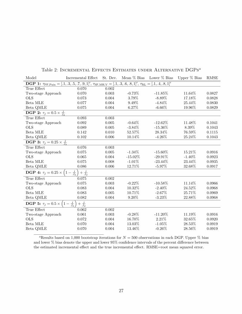
Table 2: Incremental Effects Estimates under Alternative DGPsa

Model Incremental Effect St. Dev. Mean % Bias Lower % Bias Upper % Bias RMSE

DGP 1: τPF,Pain = [.1, .3, .5, .7, .9, 1]′, τSF,MH,V = [.1, .3, .6, .8, 1]′, τRL = [.1, .4, .8, 1]′

True Effect 0.070 0.002Two-stage Approach 0.070 0.003 -0.73% -11.85% 11.64% 0.0827OLS 0.073 0.004 3.79% -8.89% 17.18% 0.0828Beta MLE 0.077 0.004 9.49% -4.84% 25.44% 0.0830Beta QMLE 0.075 0.004 6.27% -6.66% 19.96% 0.0829

DGP 2: τj = 0.5× jJd

True Effect 0.093 0.003Two-stage Approach 0.092 0.005 -0.64% -12.62% 11.48% 0.1041OLS 0.089 0.005 -3.84% -15.36% 8.39% 0.1043Beta MLE 0.142 0.010 52.57% 28.34% 76.59% 0.1115Beta QMLE 0.102 0.006 10.14% -4.26% 25.24% 0.1043

DGP 3: τj = 0.25× jJd

True Effect 0.076 0.003Two-stage Approach 0.075 0.005 -1.34% -15.60% 15.21% 0.0916OLS 0.065 0.004 -15.02% -29.91% -1.40% 0.0923Beta MLE 0.075 0.008 -1.01% -23.44% 23.44% 0.0935Beta QMLE 0.086 0.006 12.71% -5.97% 32.68% 0.0917

DGP 4: τj = 0.25×(

1− jJd

)+ j

Jd

True Effect 0.075 0.002Two-stage Approach 0.075 0.003 -0.22% -10.58% 11.14% 0.0966OLS 0.083 0.004 10.32% -2.40% 24.52% 0.0968Beta MLE 0.083 0.005 10.71% -2.67% 25.71% 0.0969Beta QMLE 0.082 0.004 9.20% -3.23% 22.88% 0.0968

DGP 5: τj = 0.5×(

1− jJd

)+ j

Jd

True Effect 0.062 0.002Two-stage Approach 0.061 0.003 -0.28% -11.20% 11.19% 0.0916OLS 0.072 0.004 16.70% 2.21% 32.65% 0.0920Beta MLE 0.070 0.004 13.03% -1.05% 28.53% 0.0919Beta QMLE 0.070 0.004 13.46% -0.26% 28.56% 0.0919

aResults based on 1,000 bootstrap iterations for N = 500 observations in each DGP. Upper % biasand lower % bias denote the upper and lower 95% confidence intervals of the percent difference betweenthe estimated incremental effect and the true incremental effect. RMSE=root mean squared error.

27

Table 3: Incremental Effects Estimates with Larger True Effecta

Model Incremental Effect St. Dev. Mean % Bias Lower % Bias Upper % Bias RMSE

DGP 3: τj = 0.25× jJd

True Effect 0.168 0.006Two-stage Approach 0.167 0.005 -0.48% -7.35% 6.17% 0.0676OLS 0.120 0.004 -28.43% -35.49% -20.96% 0.0945Beta MLE 0.137 0.009 -18.27% -29.84% -6.09% 0.0940Beta QMLE 0.216 0.008 29.11% 19.12% 39.04% 0.0698

DGP 5: τj = 0.5×(

1− jJd

)+ j

Jd

True Effect 0.111 0.002Two-stage Approach 0.112 0.002 0.28% -3.65% 4.52% 0.0688OLS 0.155 0.004 39.58% 29.10% 50.09% 0.0887Beta MLE 0.147 0.006 32.44% 21.11% 45.85% 0.0875Beta QMLE 0.142 0.003 27.71% 18.95% 36.38% 0.0864

aResults based on 1,000 bootstrap iterations for N = 500 observations in each DGP, with datasimulated using β = 5× ID×1 rather than β = 1.5× ID×1. Upper % bias and lower % bias denote theupper and lower 95% confidence intervals of the percent difference between the estimated incrementaleffect and the true incremental effect. RMSE=root mean squared error.

28

Table 4: Summary Statistics for ISSG Data (N=209)

Variable Mean StandardDeviation

Age 58.65 13.56Levels Fused 10.36 4.34

Count Percent

Female 175 84%Posterior Approach 71 34%

Baseline Post-operativeCount Percent Count Percent

Physical Functioning DomainPF=1 0 0% 0 0%PF=2 10 5% 27 13%PF=3 43 21% 61 29%PF=4 65 31% 35 17%PF=5 77 37% 74 35%PF=6 14 7% 12 6%

Role Limitations DomainRL=1 8 4% 23 11%RL=2 68 33% 80 38%RL=3 4 2% 7 3%RL=4 129 62% 99 47%

Social Functioning DomainSF=1 38 18% 79 38%SF=2 38 18% 44 21%SF=3 63 30% 50 24%SF=4 47 22% 26 12%SF=5 12 11% 10 5%

Pain DomainP=1 1 0% 15 7%P=2 12 6% 27 13%P=3 25 12% 70 33%P=4 50 24% 47 22%P=5 75 36% 35 17%P=6 46 22% 15 7%

Mental Health DomainMH=1 37 18% 83 40%MH=2 65 31% 64 31%MH=3 56 27% 34 16%MH=4 37 18% 23 11%MH=5 14 7% 5 2%

Vitality DomainV=1 4 2% 6 3%V=2 29 14% 69 33%V=3 53 25% 67 32%V=4 61 29% 37 18%V=5 62 30% 30 14%

29

Table 5: Regression Resultsa

OLS Beta Beta Ordered ProbitOLS MLE QMLE

Outcome: QALY QALY QALY PF RL SF P MH V

Age 0.00* 0.00 0.00* 0.01 -0.01** 0.01 0.01* 0.01* 0.00(0.00) (0.00) (0.00) (0.01) (0.01) (0.01) (0.01) (0.01) (0.01)

Female -0.02 -0.10 -0.07 0.01 -0.59*** 0.21 -0.15 -0.40* -0.22(0.02) (0.11) (0.10) (0.21) (0.22) (0.21) (0.20) (0.23) (0.21)

Levels Fused -0.00 -0.01 -0.01 -0.03* -0.03* -0.02 0.02 -0.01 0.01(0.00) (0.01) (0.01) (0.02) (0.02) (0.02) (0.02) (0.02) (0.02)

Posterior Approach 0.01 0.07 0.07 0.23 0.40** 0.24 0.00 0.00 0.15(0.02) (0.09) (0.09) (0.18) (0.19) (0.19) (0.18) (0.19) (0.18)

Baseline HRQoLSF-6D Index 0.57*** 2.49*** 2.54***

(0.07) (0.40) (0.37)PF 0.49***

(0.09)RL 0.36***

(0.08)SF 0.39***

(0.07)P 0.43***

(0.07)MH 0.59***

(0.08)V 0.42***

(0.07)RMSE 0.1103 .1218 0.1100 0.1099

aResults based on OLS, Beta MLE, Beta QMLE, and Ordered Probit regressions. Beta MLE andQMLE estimation follows the procedure and code available from Basu & Manca (2012). Standarderrors in parenthesis, * p<0.1. ** p<0.05. *** p<0.01. RMSE: root mean squared error.

30

Table 6: Incremental Effectsa

OLS Beta MLE Beta QMLE 2SE

Age 0.001 0.001 0.001 0.001(0.001) (0.001) (0.001) (0.001)

Female -0.016 -0.021 -0.016 -0.021(0.022) (0.024) (0.022) (0.021)

Levels Fused -0.002 -0.003 -0.002 -0.001(0.002) (0.002) (0.002) (0.002)

Posterior Approach 0.015 0.016 0.015 0.018(0.019) (0.021) (0.019) (0.018)

Baseline HRQoLPF 0.011 0.010 0.011 0.008

(0.002) (0.002) (0.001) (0.002)RL 0.000 0.000 0.000 0.005

– – – (0.001)SF 0.001 0.001 0.001 0.011

(0.000) (0.000) (0.000) (0.002)P 0.025 0.024 0.024 0.015

(0.004) (0.004) (0.003) (0.003)MH 0.000 0.000 0.000 0.015

– – – (0.002)V 0.004 0.003 0.003 0.005

(0.001) (0.001) (0.001) (0.001)

aIncremental effects on QALYs estimated via the method of recycled predictions following OLS,Beta MLE, Beta QMLE, and 2SE (Oaxaca, 1973; Graubard & Korn, 1999; Basu & Rathouz, 2005;Basu, 2005; Glick, 2007; Kleinman & Norton, 2009). Beta MLE and QMLE estimation followsthe procedure and code available from Basu & Manca (2012). Bootstrapped standard errors inparenthesis based on 1,000 iterations.

31