Pushing the Limits of the Maya Cluster - University of ...gobbert/papers/REU2014Team4.pdfPushing the...

Pushing the Limits of the Maya ClusterREU Site: Interdisciplinary Program in High Performance Computing

Adam Cunningham1, Gerald Payton2, Jack Slettebak1, Jordi Wolfson-Pou3,Graduate assistants: Jonathan Graf2, Xuan Huang2, Samuel Khuvis2,

Faculty mentor: Matthias K. Gobbert2,Clients: Thomas Salter4 and David J. Mountain4

1Department of Computer Science and Electrical Engineering, UMBC2Department of Mathematics and Statistics, UMBC

3Department of Physics, University of California, Santa Cruz4Advanced Computing Systems Research Program

Technical Report HPCF–2014–14, www.umbc.edu/hpcf > Publications

Abstract

Parallelization of code, using multiple cores/threads, and heterogeneous computing, using the CPU with other devices,has come to the forefront of computing as methods to reduce the execution time of computationally demanding algorithms.For our project, we test various hardware setups on the maya cluster at UMBC, which include multiple nodes and GPUs,by solving the Poisson equation using the conjugate gradient method. To explore these different setups, we made use ofboth industry benchmarks and our own code, which we design using the compilers native to each device and API. We findsignificant gains both in using a heterogeneous model and after parallelizing our code.

1 Introduction

The University of Maryland, Baltimore County (UMBC) High Performance Computing Facility (www.umbc.edu/hpcf) housesthe 240-node cluster maya capable of performing computationally intensive tasks using state of the art equipment. The mayacluster contains an array of cutting edge devices each of which requires a performance evaluation to explore optimal setupsand greatest total usage of hardware. Properly identifying the best setup will both shed light on the complex inner workingsof the cluster as well as improve the performance available to the diverse range of researchers who rely on it.

To test the maya cluster, we focused on using the CG (Conjugate Gradient) method, which solves a large, sparse system oflinear equations. We developed our own code for a matrix-free implementation of the CG method, and tested it by solving thePoisson test problem in two dimensions. In our tests we used both homogenous and heterogeneous computing models. For ourhomogenous tests used MPI (Message Passing Interface) for communication between nodes, testing both blocking and non-blocking communication, and a variety of different total node and total process combinations. Our heterogenous tests usedthe available K20 NVIDIA GPUs on the cluster, with an identical implementation of our CG test problem written in CUDA.We tested both serial runs of the GPUs and parallel runs of the GPU using MPI for communication from node-to-node.

Although our test problem is comprehensive, there is a clear need for a benchmark to provide more thorough, reliableresults. A benchmark is a portable program that runs a specified task on a system and returns a meaningful metric of thesystem’s performance that can be compared to existing results from other systems. We chose the Sandia High PerformanceConjugate Gradient (HPCG) benchmark to test the maya cluster, which also uses the CG method to solve the Poissonequation, here in three dimensions and with preconditioning.

The Sandia HPCG benchmark (http://software.sandia.gov/hpcg/) was created by Sandia National Laboratories tocomplement the Top 500 benchmark (www.top500.org), which is now 35 years old. Like the Top 500 benchmark, the HPCGbenchmark provides a stable, well-tested framework for benchmarking that ensures reliable results. Also, being a more recentbechmark, it was also made to better fit current high performance computing needs [2]. The benchmark publishes a list ofthe results that other clusters have attained after running the benchmark. The HPCG benchmark returns a measurement inGFLOP/s (Giga FLoating Point OPerations per second), a floating point operation being any arithmetic operation betweenstored decimal numbers. Thus, the total number of GFLOP/s can be thought of as the total computational throughputof the system, and an increase in total GFLOP/s is analagous to an increase in total power of the system. Running thebenchmark will give us results that can be compared against other similarly equipped clusters, giving a good indication ofhow much more the cluster can be improved and a useful metric of maya’s total potential in the future.

The HPCG benchmark allows for a variety of different setups that can affect runtime, including the multi-threadinglibrary OpenMP (which our code for the Poisson test problem does not include), different compiler options, and MPI formulti-node setups. Our tests used a variety of different total process and thread counts.

Section 2 of this report details the system architecture and related hardware, including the node architecture in Section 2.1and GPU architecture in Section 2.2. Section 3 outlines the test problems used for testing including our own Poisson test

1

www.umbc.edu/hpcf

www.umbc.edu/hpcf

http://software.sandia.gov/hpcg/

www.top500.org

problem, described in Section 3.1, and the Sandia HPCG benchmark, described in Section 3.2. Section 4 describes thehardware and software setups we used as well as how they were implemented. We describe our implementation for a node-only test in Section 4.1, our implementation of a serial GPU test in Section 4.2, and an implementation of a parallel GPUtest in Section 4.3, which all used our Poisson test problem to run. In Section 4.4, we detail our approach to running theHPCG benchmark. Section 5 reports the resuls we observed with Section 5.1 detailing and explaining our resuls for our nodeonly implementation of our Poisson test problem, Section 5.2 detailing our results for our serial GPU implementation of ourPoisson test problem, Section 5.3 detailing our results for our parallel GPU implementation of our Poisson test problem, andSection 5.4 detailing our results from the HPCG benchmark. In Section 6, we draw our conclusions and explain the possiblefuture experiments/applications related to the tests we performed.

2 System Specification

2.1 Node Architecture

The 72 nodes of the newest portion of maya are set up as 67 compute nodes, 2 develop nodes, 1 user node, and 1 managementnode. Figure 2.1 shows a schematic of one of the compute nodes that is made up of two eight-core 2.6 GHz Intel E5-2650v2Ivy Bridge CPUs. Each core of each CPU has dedicated 32 kB of L1 and 256 kB of L2 cache. All eight cores of each CPUshare 20 MB of L3 cache. The 64 GB of the node’s memory is formed by eight 8 GB DIMMs, four of which are connectedto each CPU. The two CPUs of a node are connected to each other by two QPI (quick path interconnect) links. The nodesin maya 2013 are connected by a quad-data rate InfiniBand interconnect.

An individual node can compile and run native C programs. However, a program can also be run in parallel acrossmultiple nodes using MPI for any data distribution between explicit processes. However, it is worth noting that parallelizingan algorithm or program is not always beneficial. While it can greatly reduce the computation time of a more computationallyintense program, based on how parallelizable the algorithm is, but communicating data can also be expensive. Therefore,there is a trade-of between calculation time and communication time, and parallel computing is most beneficial for largeproblems.

To submit a parallel job to the cluster, the user must request a specific number of nodes as well as how many processesshould be spawned on each individual node. The number of total jobs that can be spawned on a node is dictated by the totalnumber of cores available, which in the case of a maya node is 16. More information on submitting jobs to the maya clustercan be found on the UMBC HPCF website.

2.2 GPU Architecture

The NVIDIA K20 GPU (Graphics Processing Unit) is built upon a massively parallel architecture and can be used tospeed up identical calculations on independent pieces of data. This is accomplished by taking the calculations and placingthem onto the K20’s 2,496 CUDA cores and running every calculation in parallel, giving the GPU a theoretical maximumperformance of 1.2 TFLOP/s (FLOPS = FLoating OPerations per Second). The CUDA cores within the K20 are arrangedinto blocks of 192 cores, known as streaming multiprocessors (SM). While every SM has its own L1 cache, the majority of theGPU’s memory is located in a local 5 GB bank that is shared amongst all SMs. The SMs operate upon the single-instruction,multiple-data (SIMD) paradigm, as every core executes the same instruction but on an seperate, independent piece of datain memory. Figure 2.2 illustrates a high-level design of the K20 architecture.

On the software layer, a set of instructions for the GPU is written as a kernel in the CUDA language. A kernel is a singlefunction that is to be run on the GPU that needs to have specified both the number of threads/cores and blocks it is goingto be run on. In software, a block is simply a data structure that can be queued for execution on the GPU with a certainnumber of threads for execution specified. Kernels are run asynchronously, which means that it will run in the backgroundwhile the calling program continues execution. This can be problematic if the calling function relies on a kernel to returnvalues for continued execution. Once a kernel has been created and sent to the GPU, each streaming multiprocessor willexecute the kernel on data in global memory. To operate on different pieces of data, each core has an id number that cansplit the data up into different sections.

As shown in Figure 2.2 the GPU is connected to the CPU through a PCI Express bus. For the GPU to run a CUDAkernel, it must first be passed both the instructions and the data from the CPU. The latter process is often expensive and,as the amount of data gets larger, the amount of time devoted to communication can become a limiting factor in the runtimeof a program.

2

Figure 2.1: Illustration of node architecture with dual sockets shown as well as physical cores within each socket, on-chipcache, and respective memory channels.

Figure 2.2: NVIDIA K20 GPU architecture with streaming multiprocessors, compute cores, and cache shown.

2.3 Software Specification

To effectively test the hardwares listed we rely on a variety of different languages and associated compilers. For all of theparallel implementations, including the HPCG benchmark, the MVAPICH2 1.9 MPI (Message Passing Interface) C/C++library implementation is used to communicate data from node to node. To compile MPI code, the mpi.h header file mustbe included and an appropriate compiler that can recognize MPI functions calls must be used. We used mpicc for our code,which is simply the Intel compiler version 2013_sp1.1 with an MPI wrapper, to compile all of our MPI related code. Forour CUDA code, we used the nvcc compiler to compile, and compiled with the mpicc for any files with MPI function calls.

3

3 Test Problems

3.1 Poisson Test Problem

The Poisson equation is an elliptic partial differential equation. Our team will be analyzing this equation with homogeneousDirichlet boundary conditions

−∆u = f in Ω, (3.1)

u = 0 on ∂Ω, (3.2)

in the two-dimensional domain Ω with boundary ∂Ω and with the Laplace operator being defined as ∆u = ∂2u∂x1

2+ ∂2u

∂x22.

This problem is discretized by the finite difference methods using the conventional five-point stencil, which results in asystem of linear equations. Our team will implement the conjugate gradient (CG) method to solve this linear system usinga matrix-free implementation of the algorithm that computes the result of the matrix-vector product of the system matrixwith an input vector.

For each dimension, we use N + 2 mesh points and construct and uniform mesh spacing h = 1/(N + 1). The mesh pointsare defined as (xk1

, xk2) ∈ Ω ∈ R2 with xki = hki, ki = 0, 1, ..., N,N + 1 in each dimension i = 1, 2. The approximations to

the the solution at the mesh points are denoted by uk1,k2≈ u(xk1

, xk2). Consequently, the second-order derivatives in the

Laplace operator at the N2 interior mesh points are denoted by

∂2u(xk1 , xk2)

∂x21+∂2u(xk1 , xk2)

∂x22≈ uk1−1,k2 − 2uk1,k2 + uk1+1,k2

h2+uk1,k2−1 − 2uk1,k2 + uk1,k2+1

h2(3.3)

for ki = 1, ..., N , i = 1, 2 as the approximations at the interior points. These approximations combined with the boundarycondition produces a system of N2 linear equations for the finite difference approximations at the N2 interior mesh points.

When we collect the N2 approximations uk1,k2in a vector u ∈ RN2

using the natural order of the mesh points, theproblem can be stated as a system of linear equations in the form

Au = b (3.4)

with the system matrix defined as A ∈ RN2×N2

and a right-hand side vector b ∈ RN2

. Concretely we have

A =

S TT S T

. . .. . .

. . .

T S TT S

∈ RN2×N2

(3.5)

with a tri-diagonal matrix S = tridiag(−1, 4,−1) ∈ RN×N for the diagonal blocks of A and T = −I ∈ RN×N , which denotesthe negative identity matrix for the off diagonal blocks of A. The matrix A is known to be symmetric positive definite andthus the conjugate gradient method is guaranteed to converge for this problem.

We consider the elliptic problem (3.2) on the unit square with right-hand side function

f(x1, x2) = (−2π2)(

cos(2πx1) sin2(πx2) + sin2(πx1) cos(2πx2)), (3.6)

for which the solution u(x1, x2) = sin2(πx1) sin2(πx2) is known. On a mesh with 33 × 33 points and mesh spacing h =1/32 = 0.03125, the numerical solution uh(x1, x2) can be plotted vs. (x1, x2) as a mesh plot as in Figure 3.1 (a). The shapeof the solution clearly agrees with the true solution of the problem. At each mesh point, an error is incurred compared to thetrue solution u(x1, x2). A mesh plot of the error u− uh vs. (x1, x2) is plotted in Figure 3.1 (b). We see that the maximumerror occurs at the center of the domain of size about 3.2e–3, which compares well to the order of magnitude h2 ≈ 0.98e–3of the theoretically predicted error.

Table 3.1 lists the mesh resolution N of the N ×N mesh, the number of degrees of freedom N2 (DOF; i.e., the dimensionof the linear system), the norm of the finite difference error ‖u− uh‖ ≡ ‖u− uh‖L∞(Ω)

, the ratio of consecutive errors‖u− u2h‖/‖u− uh‖ , the number of conjugate gradient iterations #iter. In nearly all cases, the norms of the finite differenceerrors in Table 3.1 decrease by a factor of about 4 each time that the mesh is refined by a factor 2. This confirms that thefinite difference method is second-order convergent, as predicted by the numerical theory for the finite difference method.The fact that this convergence order is attained also confirms that the tolerance of the iterative linear solver is tight enoughto ensure a sufficiently accurate solution of the linear system.

4

(a) Numerical solution uh (b) Error u− uh

Figure 3.1: Poisson Test Problem: Mesh plots of (a) the numerical solution uh vs. (x1, x2) and (b) the error u − uhvs. (x1, x2).

Table 3.1: Poisson Test Problem: Convergence study.

N DOF ‖u− uh‖ Ratio #iter

32 1,024 3.0128e–03 N/A 4864 4,096 7.7811e–04 3.87 96

128 16,384 1.9765e–04 3.94 192256 65,536 4.9797e–05 3.97 387512 262,144 1.2494e–05 3.99 783

1024 1,048,576 3.1266e–06 4.00 1,5812048 4,194,304 7.8019e–07 4.01 3,1924096 16,777,216 1.9366e–07 4.03 6,4528192 67,108,864 4.7377e–08 4.09 13,033

3.2 Sandia HPCG Benchmark

A benchmark is a portable application that can be used globally with the intention of testing the performance of a com-puting system. The Sandia High Performance Computing Conjugate Gradient (HPCG) benchmark is a conjugate gradientbenchmark code for a 3D domain on an arbitrary number of processors. This benchmark, which is written in portable C++code, generates a 27-point finite difference matrix with sub-block sizes on each processor specified by the user, provides amore detailed description of the benchmark implementation [1].

The problem generated by this benchmark can be viewed as a stationary heat diffusion model of a single degree with zeroDirichlet boundary conditions, whose global domain dimensions are Nx ×Ny ×Nz with Nx = nxpx, Ny = nypy, Nz = nzpz,where nx × ny × nz are the local sub grid dimensions in the x-, y-, and z-dimensions, respectively, assigned to each MPIprocess with a total number of MPI processes P , which are factored into three dimensions as px × py × pz.

In the setup phase, a sparse linear system is constructed using the 27-point stencil at each of the grid points in the 3Ddomain [2]. Therefore, the equation at a given point will rely on the values at its specific location as well as the values of its 26neighboring points. For the interior points in the matrix, the setup is weakly diagonally dominant, while the boundary pointsare set up to be strictly diagonally dominant. The setup for this matrix implements the synthetic conservation principle forthe interior points and displays the impact of no Dirichlet boundary values on the boundary equations.

The resulting properties of the generated linear system include all initial guesses with a value of zero, a matching right-hand-side vector and a solution vector that is equal to one. The system matrix is a symmetric positive definite, non-singularmatrix with 27 nonzero entries per row for interior points and 18 to 7 entries for the boundary equations.

5

4 Implementation and Parallelization

4.1 C/MPI Implementation for Poisson Test Problem

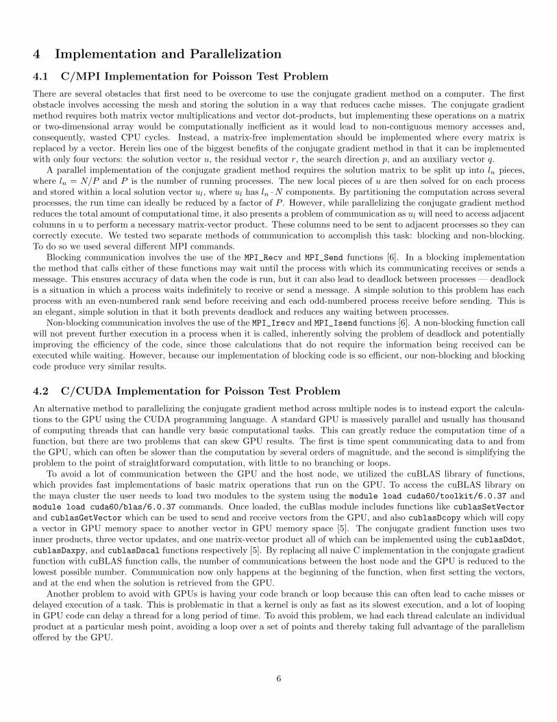
There are several obstacles that first need to be overcome to use the conjugate gradient method on a computer. The firstobstacle involves accessing the mesh and storing the solution in a way that reduces cache misses. The conjugate gradientmethod requires both matrix vector multiplications and vector dot-products, but implementing these operations on a matrixor two-dimensional array would be computationally inefficient as it would lead to non-contiguous memory accesses and,consequently, wasted CPU cycles. Instead, a matrix-free implementation should be implemented where every matrix isreplaced by a vector. Herein lies one of the biggest benefits of the conjugate gradient method in that it can be implementedwith only four vectors: the solution vector u, the residual vector r, the search direction p, and an auxiliary vector q.

A parallel implementation of the conjugate gradient method requires the solution matrix to be split up into ln pieces,where ln = N/P and P is the number of running processes. The new local pieces of u are then solved for on each processand stored within a local solution vector ul, where ul has ln ·N components. By partitioning the computation across severalprocesses, the run time can ideally be reduced by a factor of P . However, while parallelizing the conjugate gradient methodreduces the total amount of computational time, it also presents a problem of communication as ul will need to access adjacentcolumns in u to perform a necessary matrix-vector product. These columns need to be sent to adjacent processes so they cancorrectly execute. We tested two separate methods of communication to accomplish this task: blocking and non-blocking.To do so we used several different MPI commands.

Blocking communication involves the use of the MPI_Recv and MPI_Send functions [6]. In a blocking implementationthe method that calls either of these functions may wait until the process with which its communicating receives or sends amessage. This ensures accuracy of data when the code is run, but it can also lead to deadlock between processes — deadlockis a situation in which a process waits indefinitely to receive or send a message. A simple solution to this problem has eachprocess with an even-numbered rank send before receiving and each odd-numbered process receive before sending. This isan elegant, simple solution in that it both prevents deadlock and reduces any waiting between processes.

Non-blocking communication involves the use of the MPI_Irecv and MPI_Isend functions [6]. A non-blocking function callwill not prevent further execution in a process when it is called, inherently solving the problem of deadlock and potentiallyimproving the efficiency of the code, since those calculations that do not require the information being received can beexecuted while waiting. However, because our implementation of blocking code is so efficient, our non-blocking and blockingcode produce very similar results.

4.2 C/CUDA Implementation for Poisson Test Problem

An alternative method to parallelizing the conjugate gradient method across multiple nodes is to instead export the calcula-tions to the GPU using the CUDA programming language. A standard GPU is massively parallel and usually has thousandof computing threads that can handle very basic computational tasks. This can greatly reduce the computation time of afunction, but there are two problems that can skew GPU results. The first is time spent communicating data to and fromthe GPU, which can often be slower than the computation by several orders of magnitude, and the second is simplifying theproblem to the point of straightforward computation, with little to no branching or loops.

To avoid a lot of communication between the GPU and the host node, we utilized the cuBLAS library of functions,which provides fast implementations of basic matrix operations that run on the GPU. To access the cuBLAS library onthe maya cluster the user needs to load two modules to the system using the module load cuda60/toolkit/6.0.37 andmodule load cuda60/blas/6.0.37 commands. Once loaded, the cuBlas module includes functions like cublasSetVector

and cublasGetVector which can be used to send and receive vectors from the GPU, and also cublasDcopy which will copya vector in GPU memory space to another vector in GPU memory space [5]. The conjugate gradient function uses twoinner products, three vector updates, and one matrix-vector product all of which can be implemented using the cublasDdot,cublasDaxpy, and cublasDscal functions respectively [5]. By replacing all naive C implementation in the conjugate gradientfunction with cuBLAS function calls, the number of communications between the host node and the GPU is reduced to thelowest possible number. Communication now only happens at the beginning of the function, when first setting the vectors,and at the end when the solution is retrieved from the GPU.

Another problem to avoid with GPUs is having your code branch or loop because this can often lead to cache misses ordelayed execution of a task. This is problematic in that a kernel is only as fast as its slowest execution, and a lot of loopingin GPU code can delay a thread for a long period of time. To avoid this problem, we had each thread calculate an individualproduct at a particular mesh point, avoiding a loop over a set of points and thereby taking full advantage of the parallelismoffered by the GPU.

6

4.3 C/MPI/CUDA Programming

The CG function could theoretically be sped up even further by splitting the problem up across multiple nodes and thenimplementing GPU acceleration on each. This requires both the MPI interface, to communicate between nodes, and theCUDA interface, to communicate between host socket and device. To maximize performance, the resulting implementationmust then take into account all of the limiting factors and benefits associated with using GPU acceleration across severalnodes. In other words, our implementation needs MPI to pass relevant vectors between nodes, but it uses the GPU exclusivelyto do local calculations. Based on our previous results, we used blocking over non-blocking MPI calls to reduce total runtime.

4.4 Sandia HPCG Implementation

The HPCG benchmark can be downloaded from the Sandia National Laboratories website and unpacked into a local reposi-tory. Once unpacked, the QUICKSTART file gives detailed instructions on how the benchmark can be set up and executed, buta few changes were made to run on the maya cluster. Once in the directory that was set up in step 2 of the QUICKSTART file,the user should add a run.slurm to the bin directory. This should run the executable xhpcg and write the results of stdoutto slurm.out and of stderr to slurm.err.

The remaining files and directories are meant for accessing source and changing compiler flags to add or remove behaviorand libraries. Specifically, the README file includes general details on the HPCG benchmark as well as details on changingthe memory footprint of the benchmark. Another file, named INSTALL, details the appropriate command line arguments forthe benchmark’s executable and how to set flags that can be set compiler and run-time flags.

The unpacked benchmark also includes several directories. The setup directory includes various system-specific Makefilesthat are meant to be copied and used based on the system running the benchmark. These makefiles include flags to enableOpenMP and MPI. The tools directory contains a file that holds various flags for the documentation produced by the sourcefiles and the run results. Finally, The src directory contains all relevant source code for HPCG benchmark.

Once the code is compiled, runs should be done for a very short amount of time to test that the code is working. Becausethe Sandia HPCG implementation never actually converges, but rather relies on running sets of 50 iterations, the user canspecify the length of time to run the benchmark. The official benchmark must be run for at least 5 hours. The user canalso specify nx, ny, nz, and P , defined in Section 3.2. Additionally, the user can specify the number of OpenMP threads ntassigned to each process per node.

In order to compare larger problem sizes while comparing parallel performance, we designed an experiment to incorporatesmall and large problem sizes with convenient scaling for comparisons. We set nx = ny = nz and increased each dimensionby powers of 2, starting at the minimum constraint of 16 implemented in the code. We were able to go up to 128 withoutrunning into memory issues. Additionally, we picked P to have a cube root in order to maintain a global grid in a cubicshape. This resulted in P = 1, 8, 64, 512, using all possible combinations of nodes and processes. Furthermore, we limited thenumber software threads such that the product of the number of cores and threads is less than or equal to 16. For example,if 8 cores are specified, a maximum of 2 threads are used, allowing runs with 8 cores to use nt = 1 or 2. Table 4.1 shows theproblem sizes that result from our experimental design. This experimental design was not used for the official benchmark,but rather an initial performance study, only running for 60 seconds. The official benchmark should use all available nodesand cores and, as stated before, run for a much longer time than our experimental design runs.

Table 4.1: Sandia HPCG Benchmark: Number of unknowns Nx ×Ny ×Nz for a given number of MPI processes P andlocal mesh resolution nx × ny × nz.

nx × ny × nz P = 1 P = 8 P = 64 P = 51216 4,096 32,768 262,144 2,097,15232 32,768 262,144 2,097,152 16,777,21664 262,144 2,097,152 16,777,216 134,217,728

128 2,097,152 16,777,216 134,217,728 1,073,741,824

7

5 Results

5.1 Poisson Test Problem using C/MPI

We perform the same computational experiments as [4]. Organized as [4, Table 4.1], Tables 5.1 and 5.2 show the observedwall clock times for runs on all available combinations of nodes for N = 1024, 2048, 4096, and 8192. First, doubling the nodeswith the same processes per node halves the run time, approximately. for example, the behavior in either Table 5.1 and 5.2for mesh resolution 8192, going from 1 to 64 nodes with 1 process per node. Starting with a wall clock time of 01:44:30 for1 node, stepping along the row shows times 00:52:24 for 2 nodes, 00:26:30 for 4 nodes, 00:13:24 for 8 nodes, 00:06:48 for16 nodes, 00:03:27 for 32 nodes, and 00:01:32 for 64 nodes. It is clear that as the nodes are doubled, the wall clock timeis approximately halved, which can by examining other rows as well. This confirms the quality of the high-performanceInfiniBand interconnect, the network link that allows communication between nodes [4].

Stepping along columns in Tables 5.1 and 5.2 shows a more complicated behavior. For a given node count, going from1 to 2 nodes and from 2 to 4 nodes shows a decrease in run time, but not by approximately half, as expected based on thebehavior of doubling nodes. This is due to the architecture of a node, with 2 CPUs per node, and 8 cores per socket. Thetotal number of cores is denotes by process(es) per node in Tables 5.1 and 5.2. When 1, 2, 4, or 8 processes are requested,processes are not split up onto two CPUs but instead one CPU fills out all its cores. For example, requesting 1 node and 4processes per node will use four cores on one CPU and 0 cores on the other, instead of 2 on each. The difference this makesis based on the L1, L2, and L3 cache architecture as shown in Figure 2.1. For nodes in Maya, each core has its own L1 andL2 cache but all 8 cores share L3 cache. Hence, going from 1 node to 2 nodes results in decreasing the amount of data storedon the L3 cache per core, causing an increase in cache misses and a decrease in overall productivity.

Going from 4 to 8 cores raises a different problem in that there is little to no decrease in run time. This is due to therebeing only 4 memory channels per CPU. Since each node contains two 8-core CPUs, the default behavior of allocating all8 processes on one CPU results in a bottleneck when these processes attempt to access memory through only 4 memorychannels, which makes the 8 cores exhibit the behavior of 4 cores as each core competes for memory access. When a memoryaccess collision of this nature happens, a core must wait for the other to finish memory access before accessing the channel.

This slowdown is not seen when going from 8 to 16 processes per node. The reason for this is equivalent to comparing thetime difference in doubling nodes. When the number of requested processes increases above the number of cores in a singlesocket the node splits the load between the two sockets.

Tables 5.1 and 5.2 also shows that the difference between blocking and non-blocking communication is almost non-existent, with non-blocking having slightly lower wall clock time. This was due to our implementation of the clocking code.For blocking, if a process sends data to another process, it will wait for the other process to receive before continuing onto the next task in execution. In our implementation we had processes with even IDs send first and then receive, and oddprocesses receive first and then send. Because each process was only sending to its right or left neighbor, the time eachprocess waited became negligible.

Tables 5.3 and 5.4 and Figures 5.1 and 5.2 show the speedup and efficiency results of running four mesh resolutions, N= 1024, 2048, 4096, and 8192, up to 1024 processes on both blocking and non-blocking setups. The increase in number ofparallel processes used went as 2ν with ν = 0, 1, 2, ..., 10, where 1 node was used for number of parallel processes 1 to 16and 2 to 64 nodes with 16 processes was used for 32 to 1024 number of parallel processes. The dashed black lines show anoptimal trend. Speedup is calculated with Sν = T1/Tν where ν goes as 2ν for ν =1, 2,...,10. Tp is the wall clock time usingp MPI processes, and T1 is the wall clock time for 1 node with 1 process per node. Efficiency is calculated with Ep = Sp/p,where p is the number of parallel processes and Sp is the speedup corresponding to those processes. In Figures 5.1 and 5.2,the optimal trend line for speedup is simply Sp = p and Ep = 1 for efficiency

Stepping along the mesh 1024 row within either speedup sub-table (b) shows a rapid speedup decrease away from optimal,then increase to optimal, for processes 1 to 16. From processes 16 to 1024 a steady decrease is shown. These tables show thatas the mesh size increases, this dip away from the optimal trend has a greater length, but a smaller height, and can be seenin either efficiency sub-table (c). For example, stepping along a mesh 2048 row shows a dip from 1 to 64 processes, but asmaller efficiency at 64 than the efficiency of mesh 1024 at 16 processes. Mesh 4096 has a dip from 1 to 256 processes, but asmaller efficiency at 256 than the efficiency of mesh 2048 at 64. Mesh 8192 does not have a dip, only a degradation away fromoptimal. This behavior for increasing mesh size shows that as the mesh increases, this dip collapses into a curve, which isshown in sub-plots (b) of Figures 5.1 and 5.2. Furthermore, lower mesh resolutions eventually degrade faster. Hence, highermesh resolutions are more efficient at higher numbers of processes. For example, mesh resolution 8192 is less efficient for alower number of processes, but the highest in efficiency at 1024 processes. The speedup sub-plots confirms this showing thatmesh resolution 8192 follows a more linear trend while mesh resolutions 1024, 2048, and 4096 have greater speedup than 8192at lower numbers of processes, but plateau at higher numbers. This behavior is due to hardware communication. Because thecomputational intensity of mesh resolution 1024 is less than that of 8192, lower numbers of processes are suitable for 1024, and

8

Table 5.1: Poisson Test Problem: Observed wall clock time in HH:MM:SS for C/MPI of all available combinations ofnodes and processes per node for blocking communication commands.

(a) Mesh resolution N ×N = 1024× 1024, system dimension 1,048,5761 node 2 nodes 4 nodes 8 nodes 16 nodes 32 nodes 64 nodes

1 process per node 00:00:09 00:00:03 00:00:01 00:00:00 00:00:00 00:00:00 00:00:002 processes per node 00:00:05 00:00:01 00:00:00 00:00:00 00:00:00 00:00:00 00:00:004 processes per node 00:00:04 00:00:00 00:00:00 00:00:00 00:00:00 00:00:00 00:00:008 processes per node 00:00:02 00:00:00 00:00:00 00:00:00 00:00:00 00:00:00 00:00:00

16 processes per node 00:00:00 00:00:00 00:00:00 00:00:00 00:00:00 00:00:00 00:00:00

(b) Mesh resolution N ×N = 2048× 2048, system dimension 4,194,3041 node 2 nodes 4 nodes 8 nodes 16 nodes 32 nodes 64 nodes



(c) Mesh resolution N ×N = 4096× 4096, system dimension 16,777,2161 node 2 nodes 4 nodes 8 nodes 16 nodes 32 nodes 64 nodes



(d) Mesh resolution N ×N = 8192× 8192, system dimension 67,108,8641 node 2 nodes 4 nodes 8 nodes 16 nodes 32 nodes 64 nodes



higher numbers of processes are suitable for 8192. With higher processes for a mesh resolution of 1024, communication timedominates because the mesh per process is so small. For lower processes for a mesh resolution of 8192, run time is massivebecause of the computational intensity. This illustrates the power of parallel computation, showing that as a problem’scomputational intensity increases, more processes is necessary for faster calculations.

9

Table 5.2: Poisson Test Problem: Observed wall clock time in HH:MM:SS for C/MPI of all available combinations ofnodes and processes per node for non-blocking communication commands.

(a) Mesh resolution N ×N = 1024× 1024, system dimension 1,048,5761 node 2 nodes 4 nodes 8 nodes 16 nodes 32 nodes 64 nodes



(b) Mesh resolution N ×N = 2048× 2048, system dimension 4,194,3041 node 2 nodes 4 nodes 8 nodes 16 nodes 32 nodes 64 nodes



(c) Mesh resolution N ×N = 4096× 4096, system dimension 16,777,2161 node 2 nodes 4 nodes 8 nodes 16 nodes 32 nodes 64 nodes



(d) Mesh resolution N ×N = 8192× 8192, system dimension 67,108,8641 node 2 nodes 4 nodes 8 nodes 16 nodes 32 nodes 64 nodes



10

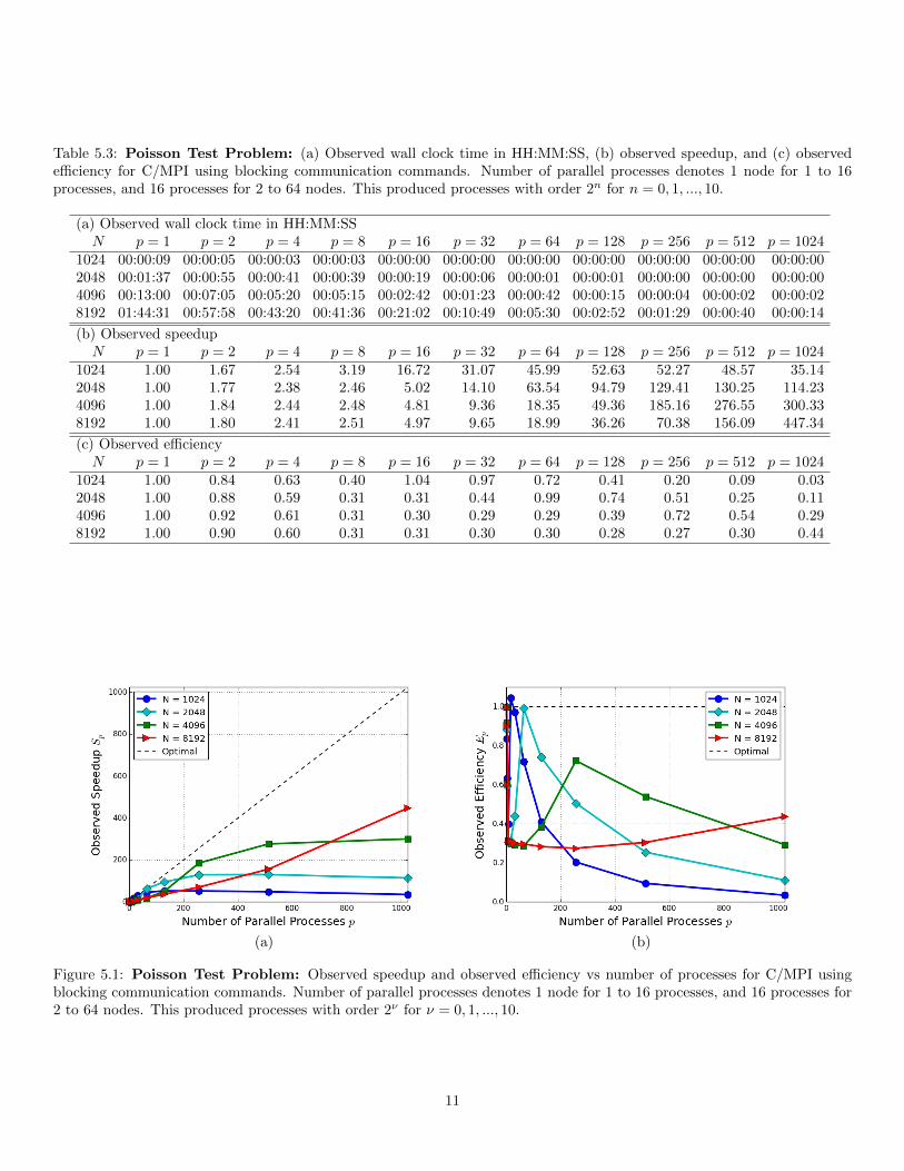
Table 5.3: Poisson Test Problem: (a) Observed wall clock time in HH:MM:SS, (b) observed speedup, and (c) observedefficiency for C/MPI using blocking communication commands. Number of parallel processes denotes 1 node for 1 to 16processes, and 16 processes for 2 to 64 nodes. This produced processes with order 2n for n = 0, 1, ..., 10.

(a) Observed wall clock time in HH:MM:SSN p = 1 p = 2 p = 4 p = 8 p = 16 p = 32 p = 64 p = 128 p = 256 p = 512 p = 1024

1024 00:00:09 00:00:05 00:00:03 00:00:03 00:00:00 00:00:00 00:00:00 00:00:00 00:00:00 00:00:00 00:00:002048 00:01:37 00:00:55 00:00:41 00:00:39 00:00:19 00:00:06 00:00:01 00:00:01 00:00:00 00:00:00 00:00:004096 00:13:00 00:07:05 00:05:20 00:05:15 00:02:42 00:01:23 00:00:42 00:00:15 00:00:04 00:00:02 00:00:028192 01:44:31 00:57:58 00:43:20 00:41:36 00:21:02 00:10:49 00:05:30 00:02:52 00:01:29 00:00:40 00:00:14

(b) Observed speedupN p = 1 p = 2 p = 4 p = 8 p = 16 p = 32 p = 64 p = 128 p = 256 p = 512 p = 1024

1024 1.00 1.67 2.54 3.19 16.72 31.07 45.99 52.63 52.27 48.57 35.142048 1.00 1.77 2.38 2.46 5.02 14.10 63.54 94.79 129.41 130.25 114.234096 1.00 1.84 2.44 2.48 4.81 9.36 18.35 49.36 185.16 276.55 300.338192 1.00 1.80 2.41 2.51 4.97 9.65 18.99 36.26 70.38 156.09 447.34

(c) Observed efficiencyN p = 1 p = 2 p = 4 p = 8 p = 16 p = 32 p = 64 p = 128 p = 256 p = 512 p = 1024

1024 1.00 0.84 0.63 0.40 1.04 0.97 0.72 0.41 0.20 0.09 0.032048 1.00 0.88 0.59 0.31 0.31 0.44 0.99 0.74 0.51 0.25 0.114096 1.00 0.92 0.61 0.31 0.30 0.29 0.29 0.39 0.72 0.54 0.298192 1.00 0.90 0.60 0.31 0.31 0.30 0.30 0.28 0.27 0.30 0.44

(a) (b)

Figure 5.1: Poisson Test Problem: Observed speedup and observed efficiency vs number of processes for C/MPI usingblocking communication commands. Number of parallel processes denotes 1 node for 1 to 16 processes, and 16 processes for2 to 64 nodes. This produced processes with order 2ν for ν = 0, 1, ..., 10.

11

Table 5.4: Poisson Test Problem: (a) Observed wall clock time in HH:MM:SS, (b) observed speedup, and (c) observedefficiency for C/MPI using non-blocking communication commands. Number of parallel processes denotes 1 node for 1 to 16processes, and 16 processes for 2 to 64 nodes. This produced processes with order 2n for n = 0, 1, ..., 10.

(a) Observed wall clock time in HH:MM:SSN p = 1 p = 2 p = 4 p = 8 p = 16 p = 32 p = 64 p = 128 p = 256 p = 512 p = 1024

1024 00:00:09 00:00:05 00:00:04 00:00:03 00:00:00 00:00:00 00:00:00 00:00:00 00:00:00 00:00:00 00:00:002048 00:01:38 00:00:56 00:00:41 00:00:40 00:00:20 00:00:06 00:00:01 00:00:00 00:00:00 00:00:00 00:00:004096 00:13:00 00:07:21 00:05:21 00:05:16 00:02:39 00:01:24 00:00:44 00:00:15 00:00:05 00:00:02 00:00:028192 01:45:12 00:57:12 00:43:25 00:41:46 00:21:01 00:10:39 00:05:26 00:02:56 00:01:28 00:00:39 00:00:13

(b) Observed speedupN p = 1 p = 2 p = 4 p = 8 p = 16 p = 32 p = 64 p = 128 p = 256 p = 512 p = 1024

1024 1.00 1.75 2.33 3.20 15.52 30.83 44.66 53.08 53.58 44.71 35.542048 1.00 1.73 2.36 2.44 4.74 14.10 61.20 101.23 119.90 140.93 129.024096 1.00 1.77 2.43 2.47 4.90 9.28 17.67 49.48 141.49 285.25 312.838192 1.00 1.84 2.42 2.52 5.00 9.86 19.33 35.66 71.60 158.59 450.95

(c) Observed efficiencyN p = 1 p = 2 p = 4 p = 8 p = 16 p = 32 p = 64 p = 128 p = 256 p = 512 p = 1024

1024 1.00 0.87 0.58 0.40 0.97 0.96 0.70 0.41 0.21 0.09 0.032048 1.00 0.86 0.59 0.31 0.30 0.44 0.96 0.79 0.47 0.28 0.134096 1.00 0.88 0.61 0.31 0.31 0.29 0.28 0.39 0.55 0.56 0.318192 1.00 0.92 0.61 0.31 0.31 0.31 0.30 0.28 0.28 0.31 0.44

(a) (b)

Figure 5.2: Poisson Test Problem: Observed speedup and observed efficiency vs number of processes for C/MPI usingnon-blocking communication commands. Number of parallel processes denotes 1 node for 1 to 16 processes, and 16 processesfor 2 to 64 nodes. This produced processes with order 2ν for ν = 0, 1, ..., 10.

12

5.2 Poisson Test Problem using CUDA

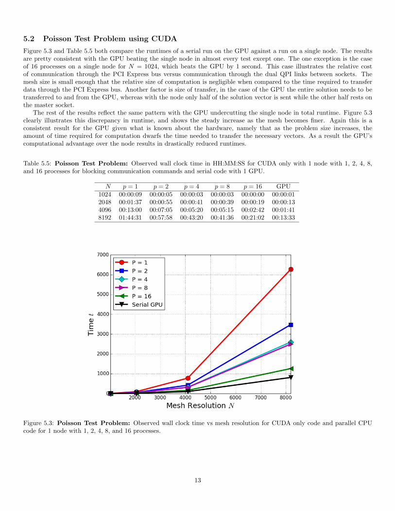
Figure 5.3 and Table 5.5 both compare the runtimes of a serial run on the GPU against a run on a single node. The resultsare pretty consistent with the GPU beating the single node in almost every test except one. The one exception is the caseof 16 processes on a single node for N = 1024, which beats the GPU by 1 second. This case illustrates the relative costof communication through the PCI Express bus versus communication through the dual QPI links between sockets. Themesh size is small enough that the relative size of computation is negligible when compared to the time required to transferdata through the PCI Express bus. Another factor is size of transfer, in the case of the GPU the entire solution needs to betransferred to and from the GPU, whereas with the node only half of the solution vector is sent while the other half rests onthe master socket.

The rest of the results reflect the same pattern with the GPU undercutting the single node in total runtime. Figure 5.3clearly illustrates this discrepancy in runtime, and shows the steady increase as the mesh becomes finer. Again this is aconsistent result for the GPU given what is known about the hardware, namely that as the problem size increases, theamount of time required for computation dwarfs the time needed to transfer the necessary vectors. As a result the GPU’scomputational advantage over the node results in drastically reduced runtimes.

Table 5.5: Poisson Test Problem: Observed wall clock time in HH:MM:SS for CUDA only with 1 node with 1, 2, 4, 8,and 16 processes for blocking communication commands and serial code with 1 GPU.

N p = 1 p = 2 p = 4 p = 8 p = 16 GPU1024 00:00:09 00:00:05 00:00:03 00:00:03 00:00:00 00:00:012048 00:01:37 00:00:55 00:00:41 00:00:39 00:00:19 00:00:134096 00:13:00 00:07:05 00:05:20 00:05:15 00:02:42 00:01:418192 01:44:31 00:57:58 00:43:20 00:41:36 00:21:02 00:13:33

Figure 5.3: Poisson Test Problem: Observed wall clock time vs mesh resolution for CUDA only code and parallel CPUcode for 1 node with 1, 2, 4, 8, and 16 processes.

13

5.3 Poisson Test Problem with CUDA and MPI

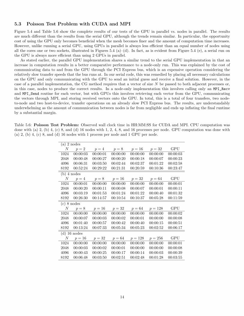
Figure 5.4 and Table 5.6 show the complete results of our tests of the GPU in parallel vs. nodes in parallel. The resultsare much different than the results from the serial GPU, although the trends remain similar. In particular, the opportunitycost of using the GPU only becomes beneficial when the mesh becomes finer and the amount of computation time increases.However, unlike running a serial GPU, using GPUs in parallel is always less efficient than an equal number of nodes usingall the cores one or two sockets, illustrated in Figures 5.4 (a)–(d). In fact, as is evident from Figure 5.4 (e), a serial run onthe GPU is always more efficient than using 2 GPUs in parallel.

As stated earlier, the parallel GPU implementation shares a similar trend to the serial GPU implementation in that anincrease in computation results in a better comparative performance to a node-only run. This was explained by the cost ofcommunicating data to and from the GPU through the PCI Express bus, which is an expensive operation considering therelatively slow transfer speeds that the bus runs at. In our serial code, this was remedied by placing all necessary calculationson the GPU and only communicating with the GPU to send an initial guess and receive a final solution. However, in thecase of a parallel implementation, the CG method requires that a vector of size N be passed to both adjacent processes or,in this case, nodes to produce the correct results. In a node-only implementation this involves calling only an MPI_Recv

and MPI_Send routine for each vector, but with GPUs this involves retrieving each vector from the GPU, communicatingthe vectors through MPI, and storing received vectors onto the GPU. In total, this is a total of four transfers, two node-to-node and two host-to-device, transfer operations on an already slow PCI Express bus. The results, are understandablyunderwhelming as the amount of communication between nodes is far from negligible and ends up inflating the final runtimeby a substantial margin.

Table 5.6: Poisson Test Problem: Observed wall clock time in HH:MM:SS for CUDA and MPI. CPU computation wasdone with (a) 2, (b) 4, (c) 8, and (d) 16 nodes with 1, 2, 4, 8, and 16 processes per node. GPU computation was done with(a) 2, (b) 4, (c) 8, and (d) 16 nodes with 1 process per node and 1 GPU per node.

(a) 2 nodesN p = 2 p = 4 p = 8 p = 16 p = 32 GPU

1024 00:00:03 00:00:01 00:00:00 00:00:00 00:00:00 00:00:032048 00:00:48 00:00:27 00:00:20 00:00:18 00:00:07 00:00:234096 00:06:31 00:03:50 00:02:44 00:02:37 00:01:22 00:02:588192 00:52:24 00:29:22 00:21:31 00:20:59 00:10:36 00:23:47

(b) 4 nodesN p = 4 p = 8 p = 16 p = 32 p = 64 GPU

1024 00:00:01 00:00:00 00:00:00 00:00:00 00:00:00 00:00:012048 00:00:20 00:00:11 00:00:08 00:00:07 00:00:01 00:00:114096 00:03:19 00:01:53 00:01:24 00:01:22 00:00:40 00:01:328192 00:26:30 00:14:57 00:10:54 00:10:37 00:05:28 00:11:59

(c) 8 nodesN p = 8 p = 16 p = 32 p = 64 p = 128 GPU

1024 00:00:00 00:00:00 00:00:00 00:00:00 00:00:00 00:00:022048 00:00:07 00:00:03 00:00:02 00:00:01 00:00:00 00:00:084096 00:01:40 00:00:57 00:00:42 00:00:40 00:00:15 00:00:518192 00:13:24 00:07:33 00:05:34 00:05:23 00:02:52 00:06:17

(d) 16 nodesN p = 16 p = 32 p = 64 p = 128 p = 256 GPU

1024 00:00:00 00:00:00 00:00:00 00:00:00 00:00:00 00:00:012048 00:00:03 00:00:02 00:00:01 00:00:00 00:00:00 00:00:084096 00:00:43 00:00:25 00:00:17 00:00:14 00:00:03 00:00:398192 00:06:48 00:03:50 00:02:51 00:02:48 00:01:28 00:03:55

14

(a) (b)

(c) (d)

(e)

Figure 5.4: Poisson Test Problem: Observed wall clock time vs. mesh resolution for CUDA and MPI, with (a) 2, (b) 4,(c) 8, and (d) 16 nodes with 1 process per node, 2 processes per node, 4 processes per node, 8 processes per node, 16 processesper node, and 1 GPU per node. Plot (e) shows results of parallel GPU code for nodes 2, 4, 8, and 16, and serial GPU code.

15

5.4 Sandia HPCG Benchmark

Tables 5.7 through 5.10 illustrate the results we received from our tests. Each of the tables represents different subgrid sizeswhere every dimension of the local subgrid is the same or nx = ny = nz ≡ n. The reported values are for n = 16, 32, 64, 128.The total thread count on every node was kept at or below 16 threads.

Our results for the Sandia HPCG benchmark mirror several trends that we had encountered before as well as some newtrends that are associated with multi-threading. Looking at Tables 5.7 to 5.10, moving down a column generally correspondsto an increase in total GFLOP/s, although the total number of processes remains the same. This is consistent with the resultsfrom our node-only implementation, namely that more processes on a single socket decreases the total L3 cache allocated toeach process resulting in more cache misses and decreased productivity.

Another trend that was mimicked from our native node-only results is the increase in computational throughput as problemsize increases. The outlier to this trend can be see in the results from Table 5.8 in which achieves the best throughput despitehaving a relatively small problem size. The most likely reason for this anomaly lies in the 20 MB (≈ 224 bytes) of on-chipL3 cache. With a local subgrid dimension of 32 × 32 × 32 and a range of total threads from nt = 1 to nt = 16, the totalnumber of grid elements on one core is between 215 and 219. Each of these elements is 8 bytes, so the total memory overheadis between 218 and 222 bytes, which can be fit entirely into cache. There is also additional memory overhead associated withthe data structures and implementation of the benchmark itself, although, looking at the results, we can assume that theproblem size with the additional memory overhead still fits into cache. Moving onto 64× 64× 64 local subgrid sizes increasesthe memory overhead to between 221 and 225 bytes, which is much more difficult to fit into cache and also adds more datafragmentation. Adding in the additional memory overhead from the data structures used in the implementation results in adataset too large for cache. Ultimately, this causes longer memory accesses and a lower total throughput.

Moving along a row on each table gives some insight into multithreading with the HPCG benchmark. Looking specificallyat the serial implementation of the benchmark, which is row (a) on Tables 5.7 to 5.10, we can see that increasing the numberof software threads running on a single core results in a loss of computational throughput or total GFLOP/s. The reasonfor this is simple, although we increase the total number of tasks in software we are not actually increasing the degreeof parallelism in the program. This is simply because a single core, without hyper-threading, has access to only a singleexecution unit, and as a result only one software thread can run at a time on a core. The slowdown is a direct result of thecore having its cache split between threads and the added overhead of the operating system timesharing multiple processeson a single core. Both of these waste CPU cycles that could be otherwise used for computation, resulting in a lower totalthroughput.

For sufficiently many processes P = 512, we see that multi-threading eventually pays off by 2 threads performing betterthan 1 thread. For the larger problem sizes in Tables 5.9–5.10, we obtain results of about 240 GFLOP/s. These results areobtained when using 64 nodes with the combination of pN = 8 processes per node and nt = 2 threads per process.

16

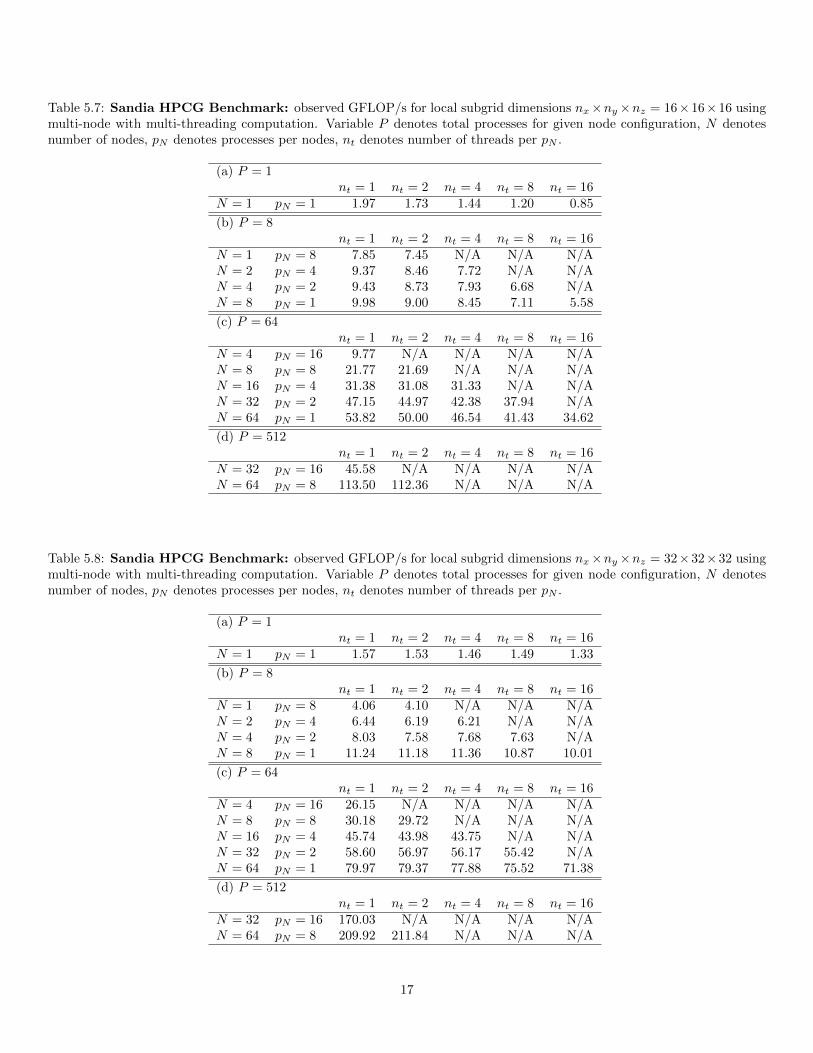
Table 5.7: Sandia HPCG Benchmark: observed GFLOP/s for local subgrid dimensions nx×ny×nz = 16×16×16 usingmulti-node with multi-threading computation. Variable P denotes total processes for given node configuration, N denotesnumber of nodes, pN denotes processes per nodes, nt denotes number of threads per pN .

(a) P = 1nt = 1 nt = 2 nt = 4 nt = 8 nt = 16

N = 1 pN = 1 1.97 1.73 1.44 1.20 0.85

(b) P = 8nt = 1 nt = 2 nt = 4 nt = 8 nt = 16

N = 1 pN = 8 7.85 7.45 N/A N/A N/AN = 2 pN = 4 9.37 8.46 7.72 N/A N/AN = 4 pN = 2 9.43 8.73 7.93 6.68 N/AN = 8 pN = 1 9.98 9.00 8.45 7.11 5.58

(c) P = 64nt = 1 nt = 2 nt = 4 nt = 8 nt = 16

N = 4 pN = 16 9.77 N/A N/A N/A N/AN = 8 pN = 8 21.77 21.69 N/A N/A N/AN = 16 pN = 4 31.38 31.08 31.33 N/A N/AN = 32 pN = 2 47.15 44.97 42.38 37.94 N/AN = 64 pN = 1 53.82 50.00 46.54 41.43 34.62

(d) P = 512nt = 1 nt = 2 nt = 4 nt = 8 nt = 16

N = 32 pN = 16 45.58 N/A N/A N/A N/AN = 64 pN = 8 113.50 112.36 N/A N/A N/A


(a) P = 1nt = 1 nt = 2 nt = 4 nt = 8 nt = 16

N = 1 pN = 1 1.57 1.53 1.46 1.49 1.33

(b) P = 8nt = 1 nt = 2 nt = 4 nt = 8 nt = 16


(c) P = 64nt = 1 nt = 2 nt = 4 nt = 8 nt = 16


(d) P = 512nt = 1 nt = 2 nt = 4 nt = 8 nt = 16


17


(a) P = 1nt = 1 nt = 2 nt = 4 nt = 8 nt = 16

N = 1 pN = 1 1.01 1.02 1.00 0.99 0.98

(b) P = 8nt = 1 nt = 2 nt = 4 nt = 8 nt = 16


(c) P = 64nt = 1 nt = 2 nt = 4 nt = 8 nt = 16


(d) P = 512nt = 1 nt = 2 nt = 4 nt = 8 nt = 16


Table 5.10: Sandia HPCG Benchmark: observed GFLOP/s for local subgrid dimensions nx × ny × nz = 128× 128× 128using multi-node with multi-threading computation. Variable P denotes total processes for given node configuration, Ndenotes number of nodes, pN denotes processes per nodes, nt denotes number of threads per pN .

(a) P = 1nt = 1 nt = 2 nt = 4 nt = 8 nt = 16

N = 1 pN = 1 1.06 1.06 1.05 1.06 1.05

(b) P = 8nt = 1 nt = 2 nt = 4 nt = 8 nt = 16


(c) P = 64nt = 1 nt = 2 nt = 4 nt = 8 nt = 16


(d) P = 512nt = 1 nt = 2 nt = 4 nt = 8 nt = 16


18

6 Conclusions

The purpose of our studies was to test the available hardware on the maya cluster and find out which setups provided optimalperformance on a specified computational problem. Our tests and benchmarks covered a wide breadth of setups and theresults we found both accomplished our original project goal and shed light on the inner workings of the hardware for futureexperiments.

To begin, we tested both serial and hardware CPU-only setups on the cluster using our own CG code. We found thatparallel runs provided significant speedups over serial runs, although they did not scale to the theoretical optimal performance.It was also found to be more efficient to use more nodes rather than more processes on a node to reduce the amount of L3cache sharing within a node’s socket. We also found that our parallel implementation achieved essentially identical resultsregardless of whether blocking or non-blocking MPI calls were used. This was mainly a result of our implementation whichensured that blocking calls would finish almost immediately.

We also tested the available NVIDIA K20 GPUs in a heterogeneous computing model, implementing both parallel andserial implementations. We found that the serial GPU implementation could provide significantly faster results than aequivalent CPU-only setup, and the gains in performance were maximized as problem size and amount of total calculationsincreased. The parallel implementation of the GPUs was not as successful and could not compete with the equivalentCPU-only setups simply because communicating necessary data from one GPU to another was very expensive.

The last test we ran used the Sandia High Performance Conjugate Gradient benchmark. In our tests we used both MPIto handle cluster-level parallelism and OpenMP to handle core-level parallelism. The results for our tests were consistent andreflected both knowledge gained from previous tests as well as new discoveries. Similar to our CPU-only implementation ofCG, the Sandia benchmark received the best performance when total nodes were increased and, therefore, the total degreeof cache sharing was reduced. In addition, we found that increasing the total of threads running on a single core, withhyperthreading disabled, was detrimental to the total throughput of the benchmark, as the thread would fight for executiontime on the core.

Overall, our tests were quite successful, both affirming and revealing several aspects of the maya cluster. Firstly, theyaffirm that parallel implementations of algorithms can provide substantial performance benefits. Secondly, they reveal thepotential of using heterogeneous computing and the gains in performance that can be had if properly implemented. Lastly,our benchmark tests revealed important facts about processes running locally on a node and how a user can best setup aproblem to run optimally on the cluster.

Our results are also important in the broader context of the HPCG benchmark, which recently published a list of clustersthat had run the benchmark [3]. The list features clusters from around the world and reports their total throughput inPFLOP/s, each of which is equivalent to 106 GFLOP/s. Most notably, at the top of the list, is a cluster that uses theIntel Phi in its tests of the benchmark, indicating that an integration of the Phi into the benchmark is both plausible andbeneficial. It is also worth noting that the TiTech cluster, the final entry on the list, contains a similar number of cores to themaya cluster (≈ 2,512 vs. 2,720) and reports 0.003700 PFLOP/s = 3,700 GFLOP/s using an optimized implementation ofthe benchmark code, indicative of the theoretical performance available. Using our best result that is obtained on 64 nodeswith 16 processes per node, or 1,024 cores, which gave us approximately 240 GFLOP/s, we can now develop a comparison:If TiTech only used 1,024 cores instead of 2,720, it would likely have a result of 1,393 GFLOP/s. This means that our resulton maya with the unoptimized implementation of the benchmark is within a factor of six.

Our results are promising, considering the use of the unoptimized implementation, and point to the opportunity for moreexperimentation with other run configurations. As demonstrated by other entries on the benchmark list, using the Intel Phisin maya could also substantially improve our results and provide us with valuable context on how the cluster performs.

Acknowledgments

These results were obtained as part of the REU Site: Interdisciplinary Program in High Performance Computing (www.umbc.edu/hpcreu) in the Department of Mathematics and Statistics at the University of Maryland, Baltimore County (UMBC) inSummer 2014. This program is funded jointly by the National Science Foundation and the National Security Agency (NSFgrant no. DMS–1156976), with additional support from UMBC, the Department of Mathematics and Statistics, the Center forInterdisciplinary Research and Consulting (CIRC), and the UMBC High Performance Computing Facility (HPCF). HPCF issupported by the U.S. National Science Foundation through the MRI program (grant nos. CNS–0821258 and CNS–1228778)and the SCREMS program (grant no. DMS–0821311), with additional substantial support from UMBC. Co-authors AdamCunningham, Gerald Payton, and Jack Slettebak were supported, in part, by the UMBC National Security Agency (NSA)Scholars Program through a contract with the NSA. Co-authors Jonathan Graf, Xuan Huang, and Samuel Khuvis weresupported during Summer 2014 by UMBC.

19

www.umbc.edu/hpcreu

www.umbc.edu/hpcreu

References

[1] Jack Dongarra and Michael A. Heroux. Toward a new metric for ranking high performance computing systems. Tech-nical Report SAND2013–4744, Sandia National Laboratories, June 2013. https://software.sandia.gov/hpcg/doc/

HPCG-Benchmark.pdf, accessed on August 08, 2014.

[2] Michael A. Heroux, Jack Dongarra, and Piotr Luszczek. HPCG technical specification. Technical Report SAND2013–8752, Sandia National Laboratories, October 2013. https://software.sandia.gov/hpcg/doc/HPCG-Specification.

pdf, accessed on August 08, 2014.

[3] Michael A. Heroux, Jack Dongarra, and Piotr Luszczek. High performance rankings, June 2014. https://software.

sandia.gov/hpcg/2014-06-hpcg-list.pdf, accessed on August 08, 2014.

[4] Samuel Khuvis and Matthias K. Gobbert. Parallel performance studies for an elliptic test problem on the clustermaya. Technical Report HPCF–2014–6, UMBC High Performance Computing Facility, University of Maryland, Bal-timore County, 2014.

[5] NVIDIA. CUDA toolkit documentation: cuBLAS, 2014. http://docs.nvidia.com/cuda/cublas/index.html#

axzz3EG7RPAmX, accessed on September 24, 2014.

[6] Peter Pacheco. Parallel Programming with MPI. Morgan Kaufmann Publishers Inc., 1997.

20

https://software.sandia.gov/hpcg/doc/HPCG-Benchmark.pdf

https://software.sandia.gov/hpcg/doc/HPCG-Benchmark.pdf

https://software.sandia.gov/hpcg/doc/HPCG-Specification.pdf

https://software.sandia.gov/hpcg/doc/HPCG-Specification.pdf

https://software.sandia.gov/hpcg/2014-06-hpcg-list.pdf

https://software.sandia.gov/hpcg/2014-06-hpcg-list.pdf

http://docs.nvidia.com/cuda/cublas/index.html#axzz3EG7RPAmX

http://docs.nvidia.com/cuda/cublas/index.html#axzz3EG7RPAmX

Pushing the Limits of the Maya Cluster - University of ...gobbert/papers/REU2014Team4.pdfPushing the...

Documents

Transcript of Pushing the Limits of the Maya Cluster - University of ...gobbert/papers/REU2014Team4.pdfPushing the...