Purely Financial Synergies and the Optimal Scope of the Firm:

Implications for Mergers, Spin-Offs, and Structured Finance

July 26, 2005

Abstract

We consider multiple activities with imperfectly correlated cash flows and zero operational synergies. These activities may be separated financially (through separate incorporation or the use of special purpose entities), allowing each to optimize its financial structure, or merged into an entity with a single optimal financial structure.

In the presence of corporate taxes and default costs, mergers can realize purely financial synergies due to reduced risk and the potential for greater leverage, as suggested by Lewellen (1971). But his conclusion that mergers always create positive financial synergies is incorrect: when firms have quite different risks or default costs, the loss from no longer being able to fit different capital structure policies to separate activities may exceed the gain from diversification. C

Characteristics of activities that gain from combination or separation are identified, and the magnitudes of gains are examined assuming normally distributed cash flows and a simple model of optimal capital structure. The results have direct application to mergers and spin-offs, and provide a rationale for structured finance techniques such as asset securitization and project finance.

JEL Classification Codes: G32, G34

2

1. Introduction

Decisions that alter the scope of the firm are amongst the most important faced by management, and amongst

the most studied by academics. Mergers and spin-offs are classic examples of such decisions. More recently,

structured finance has seen explosive growth.1 Asset securitization exceeded $6.8 trillion at year-end 2004. Esty

(2002) reports that in 2001, more than half of capital investments with cost exceeding $500 million were financed on

a separate project basis.

Positive or negative operational synergies are often cited as a prime motivation for decisions that change the

scope of the firm. A rich literature addresses the roles of economies of scope and scale, market power, incomplete

contracting, property rights, and agency costs in determining the optimal boundaries of the firm.2 Yet such

operational synergies seem difficult to identify in the case of asset securitization and structured finance.

This paper examines the existence and extent of purely financial synergies. To facilitate this objective, it is

assumed that the operational cash flow of the combined activities is nonsynergistic. If operational synergies exist,

their effect will be incremental to the financial synergies examined here.3

In a Modigliani-Miller (1958) world without taxes, bankruptcy costs, informational asymmetries, or agency

costs, there are no purely financial synergies. Capital structure is irrelevant to total firm value. But in a world with

taxes and default costs, capital structure matters. Therefore changes in the scope of the firm, which affect optimal

capital structure, will typically create financial synergies.

Financial synergies can be positive (favoring mergers) or negative (favoring separation). When activities’

cash flows are imperfectly correlated, risk can be lowered via a merger or initial consolidation. Lower risk will 1 “Structured finance” typically refers to the transfer of a subset of a company’s assets (which we term an “activity”) into a bankruptcy-remote corporation, or a special purpose vehicle or entity (SPV/SPE). These entities then offer multiple classes of securities (a “pay through” structure). Structured finance techniques include asset securitization and project finance and are discussed in more detail in Section 7. See Esty (2002, 2003, 2004), Gorton and Souleles (2005), Kleimeir and Megginson (1999), Oldfield (1997), Oldfield (2000), and Skarabot (2002). 2 Classic studies include Coase (1937), Williamson (1975), and Grossman and Hart (1986). See also Holmstrom and Roberts (1998) and the references cited therein. 3 The assumption that operational cash flows are additive, and therefore invariant to firm scope, parallels the Modigliani-Miller (1958) assumption that cash flows are invariant to changes in capital structure. While much of subsequent capital structure theory has dealt with relaxing this M-M assumption, it still stands as the base from which extensions are made.

3

reduce expected default costs. Leverage can potentially be increased, with greater tax benefits, as first suggested by

Lewellen (1971). However, Lewellen asserts that the purely financial benefits of mergers always are positive, a

widely-cited contention that is shown below to be incorrect. Financial separation of activities—whether through

separate incorporation or special purpose entity—allows each activity to have its appropriate capital structure, with an

optimal amount of debt and equity. Separate capital structures and separate limited liabilities may allow greater

financial benefits than when activities are merged with the resultant single capital structure and limited liability

shelter.4 We show that this is likely to be the case when activities differ markedly in risk. Separate capital structures

may permit greater leverage. Further, as noted by Sarig (1985), separation bestows the advantage of multiple limited

liability shelters that allow corporations to avoid negative cash flow values.

This paper examines three questions using a simple tradeoff model of capital structure:

(i) What are the characteristics of activities that benefit from merger versus separation?

(ii) How important are the magnitudes of potential financial synergies?

(iii) How do synergies depend upon the riskiness and correlation of cash flows, tax rates, default costs,

and relative size?

While operational synergies may exceed financial synergies in many mergers or spin-offs, financial synergies

can be sizable in situations that are identified. Indeed, financial synergies are often the principal reason cited for the

use of structured finance, and our model shows potentially significant financial benefits to using these techniques.

The results have implications for empirical work attempting to explain the sources of merger gains or to predict

merger activity. Aspects of firms’ cash flows which create substantial financial synergies, such as differences in

volatility and differences in default costs, should be included as possible explanatory variables.

The paper is organized as follows. Section 2 summarizes previous work on financial synergies. Section 3

introduces a simple two-period valuation model. Closed form valuation formulas when cash flows are normally

distributed are derived in Section 4, and properties of optimal capital structure are considered. Section 5 introduces

measures of financial synergies from mergers. Section 6 examines the nature and extent of synergies when cash flows

4 The analysis considers a single class of debt for each separate firm. Multiple seniorities of debt within a firm will not affect the results as long as all classes have potential recourse to the firm’s total assets.

4

are jointly normal. This section contains our core results, including a counterexample to Lewellen’s (1971) conjecture

that financial synergies are always positive. Section 7 considers spin-offs and structured finance, providing examples

that illustrate the benefits of asset securitization and project finance. Section 8 examines the distribution of benefits

between stockholders and bondholders. Section 9 concludes, and identifies several testable hypotheses.

2. Previous Work

Numerous theoretical and empirical studies have considered the effects of conglomerate mergers and

diversification. Lewellen (1971) correctly argues that combining imperfectly correlated assets, while not value-

enhancing per se, has a coinsurance effect: it reduces the risk of default, and thereby increases a measure of debt

capacity. He then asserts that higher debt capacity (by his measure) will lead to greater optimal leverage, tax savings,

and value for the merged firm. Stapleton (1982) uses a slightly different definition of debt capacity but also states that

mergers always have a positive effect on total firm value. In Section 6 below we quantify the coinsurance effect, and

show that it does not always overcome the disadvantage of forcing a single financial structure onto multiple activities.

When the latter dominates, separation rather than merger creates greater total value.

Higgins and Schall (1975), Kim and McConnell (1977), and Stapleton (1982) consider the distribution of

merger gains between extant bondholders and stockholders. They argue that while total firm value may increase with

mergers due to lower risk, bondholders may gain at shareholders’ expense. Like Lewellen’s work, these papers do

not have an explicit model of optimal capital structure before and after mergers. Therefore their conclusions about the

sign and distribution of financial synergies are incomplete.

Examples in the papers above presume that activities’ future cash flow values are always positive. In this

case, firm cash flow values will also be positive and strictly additive, and limited firm liability has no value. But Sarig

(1985) notes that, if (and only if) activities’ future cash flow values can be negative, limited firm liability provides a

valuable option to “walk away” from future activity losses.5 Mergers may incur a value loss in this case, because the

sum of separate cash flow values, with limited liability on the sum, can be less (but never more) than the sum of

5 Sarig cites the potential liabilities of tobacco and asbestos companies as examples where activity cash flows can be negative.

5

values that each have separate limited liability. Unlike additive activity cash flow values, firm cash flow values are

subadditive. We term the loss in value that results from the loss of separate firm limited liability “the Sarig effect.”

Its magnitude depends upon the distribution of activities’ future cash flows, and is independent of capital structure. It

is negligible in some of the cases that we (and other cited papers) examine. But later sections show that the Sarig

effect can be substantial under realistic circumstances.

Numerous papers have considered the potential impact of firm scope on operational synergies. Flannery,

Houston, and Venkataraman (1993) consider investors who issue external debt and equity to invest in risky projects,

and must decide upon separate or joint incorporation of the projects. Like us, they find that joint incorporation is

more valuable when project returns have similar volatility and lower correlation. But operational rather than financial

synergies drive their conclusions: investment and therefore the cash flows of the merged firm will be different than

the sum of investments and cash flows of the separate firms. John (1993) uses a related approach to analyze spin-offs,

while Chammanur and John (1996) use managerial ability and control issues to explain project finance and the scope

of the firm.

Several recent papers use an incomplete contracting approach to determining firm scope. Inderst and Müller

(2003) assume nonverifiable cash flows and examine investment decisions. Separation of activities may be

financially desirable, but only if there are increasing returns to scale for second-period investment. While cash flows

are additive in the first period, investment levels and therefore operational cash flows in the second period depend

upon whether activities are merged (centralized) or separated (decentralized). Faure-Grimaud and Inderst (2004) also

consider nonverifiable cash flows in the context of mergers. In contrast with our model, firms’ access to external

finance is restricted because of nonverifiability. Mergers affect these financing constraints and in turn affect future

cash flows. Chemla (2005) introduces an incomplete contracting environment where ex post takeovers can affect ex

ante effort by stakeholders, and therefore future operational cash flows are functions of the likelihood of takeover.

Rhodes-Kropf and Robinson (2004) focus on incomplete contracting and asset complementarity (implying operational

synergies) in explaining merger benefits. They find empirical evidence that similar firms merge. Our results (e.g.

Proposition 4 in Section 6.3) suggest financial synergies could also explain the merger of similar firms.

6

Morellec and Zhdanov (2004) use a continuous time model to consider mergers as exchange options. Positive

operational synergies are assumed but are not explicitly examined; their focus is on the dynamic evolution of firm

values and the timing of mergers.

Numerous papers have considered possible negative operational synergies arising from managerial agency

costs, including the misallocation of internal capital, that lead to a “conglomerate discount.”6 There is a rich but still

inconclusive empirical literature testing whether such a discount exists.7

The synergies we consider are in most cases supplemental to, rather than competitive with, the synergies

considered above. The cited works generally do not focus on taxes, default costs, and optimal capital structure, which

are the key source of financial synergies in our paper. Our approach is simple: information is symmetric and

verifiable, and there are no agency costs. Despite its lack of complexity, our model shows that financial synergies can

be of significant magnitude, and provides a rationale for asset securitization and project finance.

3. A Two-Period Model of Capital Structure

The analysis of financial synergies requires a model of optimal capital structure. In this section we develop a

simple two-period model to value debt and equity. The approach is related to the two-period models of DeAngelo and

Masulis (1980) and Kale, Noe, and Ramirez (1991). In contrast with these authors, we distinguish between activity

cash flow and corporate cash flow, since the latter reflects limited liability and is affected by the boundaries of the

firm. Also in contrast with these authors, our analysis makes the more realistic assumption that only interest expenses

are tax deductible. This, however, creates an endogeneity problem. When interest only is deductible, the fraction of

debt service attributed to interest payments depends on the value of the debt, which in turn depends on the fraction of 6 See, for example, Jensen (1986), Aron (1988), Rotemberg and Saloner (1994), Harris, Kriebel, and Raviv (1982), Shah and Thakor (1987), John and John (1991), John (1993), Li and Li (1996), Stein (1997), Rajan, Servaes, and Zingales (2000), and Scharfstein and Stein (2000). Maksimovic and Philips (2001) focus on inefficiencies (that generate negative cash flow synergies) of conglomerates in a model that does not include agency costs. 7 Martin and Sayrak (2003) provide a useful summary of this research. Berger and Ofek (1995) suggest conglomerate discounts on the order of 15%. This and related results have been challenged on the basis that diversified firms trade at a discount prior to diversifying: see Lang and Stulz (1994), Campa and Kedia (2002), and Graham, Lemmon, and Wolf (2002). Mansi and Reeb (2002) conclude that the conglomerate discount of total firm value is insignificantly different from zero, when debt is priced at market rather than book value.

7

debt service attributed to interest payments. We use numerical techniques to find optimal leverage. But the lack of

closed form solutions limits the comparative static results that can be obtained analytically.

3.1 Operational Cash Flows, Taxes, and Limited Liability of the Firm

We consider a risk-neutral environment with two periods t = {0, T}, where T is the length of time spanned by

the periods. The riskfree interest rate over the time period T is rT. An activity generates a random future operational

cash flow value X at time t = T. Following Sarig (1985) we allow the possibility that future operational cash flows,

and cash flow values, may be negative.

Risk neutrality implies that the value X0 of the operational cash flow at t = 0 is its discounted expected value:

(1) ∫∞

∞−+= )(

)1(1

0 XdFXr

XT

,

where F(X) is the cumulative probability distribution of X at t = T. We do not require that claims to operational cash

flows be traded.

With limited liability, the firm’s owners can “walk away” from negative cash flows through the bankruptcy

process. Thus the (pre-tax) value of the activity with limited liability is

(2) ,)()1(

1

00 ∫

∞

+= XdFX

rH

T

and the pre-tax value of limited liability is

(3) .0)(

)1(1 0

000

≥+

−=

−=

∫∞−

XdFXr

XHL

T

Obviously L0 = 0 if the probability of negative future cash flows value is zero.

Now consider an unlevered firm with limited liability when future cash flows are taxed at rate τ..8 The after-

tax value of the unlevered firm is

8 When there are personal taxes, τ will typically be less than the corporate income tax rate (currently 35%). See footnote 15.

8

(4)

,)1(

)()1()1(

1

0

00

H

XdFXr

VT

τ

τ

−=

−+

= ∫∞

.

and the present value of taxes paid by the firm (with no debt) is

(5) .)0( 00 HT τ=

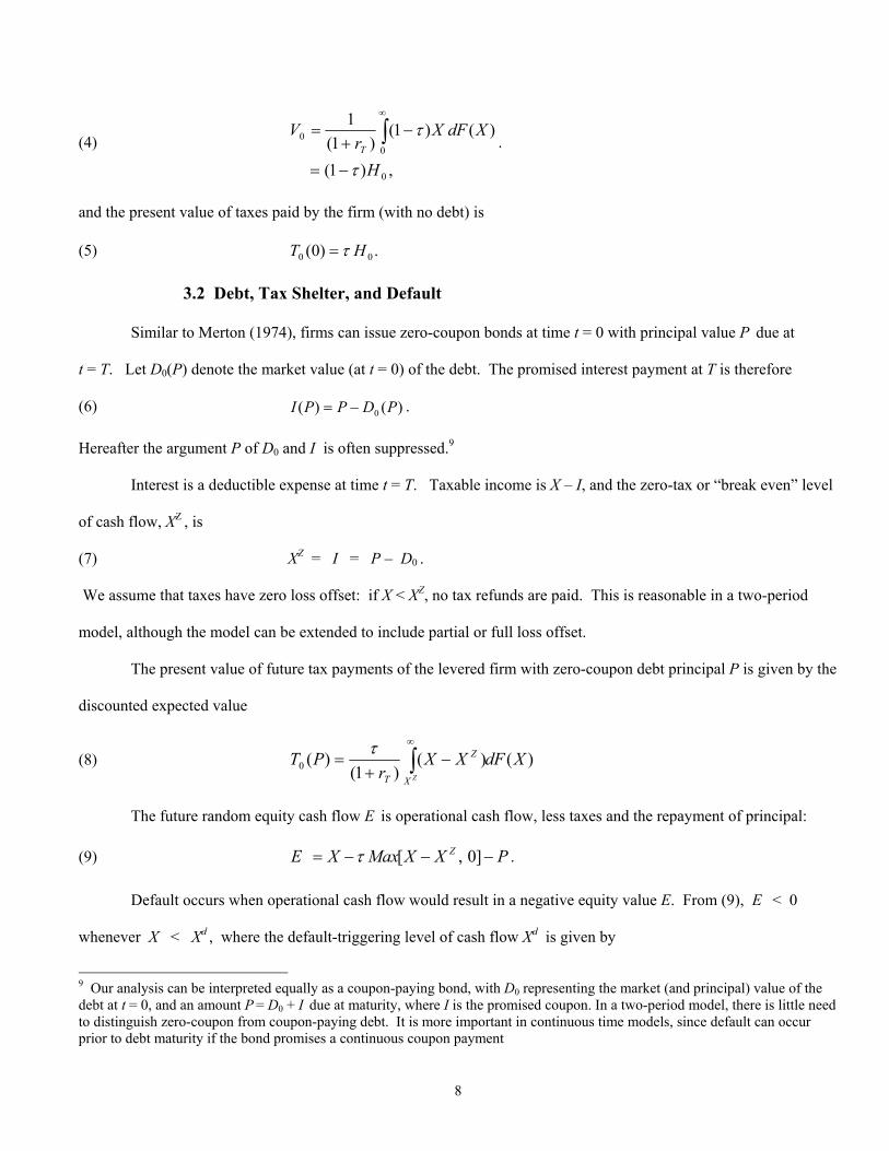
3.2 Debt, Tax Shelter, and Default

Similar to Merton (1974), firms can issue zero-coupon bonds at time t = 0 with principal value P due at

t = T. Let D0(P) denote the market value (at t = 0) of the debt. The promised interest payment at T is therefore

(6) )()( 0 PDPPI −= .

Hereafter the argument P of D0 and I is often suppressed.9

Interest is a deductible expense at time t = T. Taxable income is X – I, and the zero-tax or “break even” level

of cash flow, XZ , is

(7) XZ = I = P – D0 .

We assume that taxes have zero loss offset: if X < XZ, no tax refunds are paid. This is reasonable in a two-period

model, although the model can be extended to include partial or full loss offset.

The present value of future tax payments of the levered firm with zero-coupon debt principal P is given by the

discounted expected value

(8) )()()1(

)(0 XdFXXr

PTZX

Z

T∫∞

−+

=τ

The future random equity cash flow E is operational cash flow, less taxes and the repayment of principal:

(9) PXXMaxXE Z −−−= ]0,[τ .

Default occurs when operational cash flow would result in a negative equity value E. From (9), E < 0

whenever X < Xd , where the default-triggering level of cash flow Xd is given by

9 Our analysis can be interpreted equally as a coupon-paying bond, with D0 representing the market (and principal) value of the debt at t = 0, and an amount P = D0 + I due at maturity, where I is the promised coupon. In a two-period model, there is little need to distinguish zero-coupon from coupon-paying debt. It is more important in continuous time models, since default can occur prior to debt maturity if the bond promises a continuous coupon payment

9

(10) ]0,[ Zdd XXMaxPX −+= τ .

But it can be shown that Xd ≥ XZ. For assume that XZ > Xd. Then from equation (10), Xd = P. But from equation

(7), XZ = P – D0 ≤ P = Xd, a contradiction. It therefore follows from (10) that

(11) ,

)1(

),(

0DPX

implyingXXPX

d

Zdd

ττ

τ

−+=

−+=.

where the second line uses equation (7).

Given XZ and Xd from (7) and (11), we can now determine D0(P), the value of zero-coupon debt given the

principal P. The cash flows D to bondholders at time t = T will equal P when X ≥ Xd and the firm is solvent. In the

event of default, we assume that bondholders will receive a fraction (1 - α) of pre-tax operational cash flow value X ≥

0, where α is the fraction of cash flow value lost due to default costs.10 Recalling that the government has priority for

tax payments before bondholders, bondholders will absorb a tax liability τ (X – XZ ) in default when XZ ≤ X ≤ Xd.

Our treatment of taxes in bankruptcy is consistent with bondholders retaining the full interest rate deduction

when determining taxes owed in default. This is termed the “interest first” repayment regime, and is analyzed by

Baron (1975). An alternative considered by Turnbull (1979), the “principal first” repayment regime, is more

complex. Partial payments to debt are treated first as principal, with the remainder (if any) as interest. Talmor,

Haugen, and Barnea (1985) (TLB) suggest that optimal leverage can be quite sensitive to the repayment regime, but

we limit our analysis here to the simpler “interest first” case. TLB ignore default costs and find corner solutions often

prevail for optimal leverage under either regime. With realistic levels of default costs, we find interior solutions to

optimal leverage (see Section 4).

The present value of debt is given by

10 Note that at X = Xd – epsilon (implying default), the value received by bondholders must not exceed their promised value P. Thus, α must be sufficiently large that ((1- α)Xd - τ (Xd - XZ )) ≤ P. Our examples below satisfy this constraint, when α is chosen to match observed recovery rates.

10

(12) T

X

X

ZX

X

r

XdFXXXdFXXdFPPD

d

Z

d

d

+

−−−+

=∫∫∫

∞

1

)()()()1()()( 0

0

τα

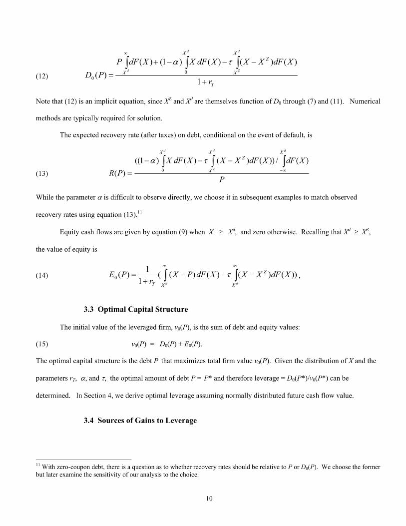
Note that (12) is an implicit equation, since XZ and Xd are themselves function of D0 through (7) and (11). Numerical

methods are typically required for solution.

The expected recovery rate (after taxes) on debt, conditional on the event of default, is

(13) P

XdFXdFXXXdFXPR

d

Z

dd X

X

XZ

X

∫ ∫∫∞−

−−−

=

)(/))()()()1(()( 0

τα

While the parameter α is difficult to observe directly, we choose it in subsequent examples to match observed

recovery rates using equation (13).11

Equity cash flows are given by equation (9) when X ≥ Xd, and zero otherwise. Recalling that Xd ≥ XZ,

the value of equity is

(14) ))()()()((1

1)(0 XdFXXXdFPXr

PE Z

X XT d d

−−−+

= ∫ ∫∞ ∞

τ ,

3.3 Optimal Capital Structure

The initial value of the leveraged firm, v0(P), is the sum of debt and equity values:

(15) v0(P) = D0(P) + E0(P).

The optimal capital structure is the debt P that maximizes total firm value v0(P). Given the distribution of X and the

parameters rT, α, and τ, the optimal amount of debt P = P* and therefore leverage = D0(P*)/v0(P*) can be

determined. In Section 4, we derive optimal leverage assuming normally distributed future cash flow value.

3.4 Sources of Gains to Leverage

11 With zero-coupon debt, there is a question as to whether recovery rates should be relative to P or D0(P). We choose the former but later examine the sensitivity of our analysis to the choice.

11

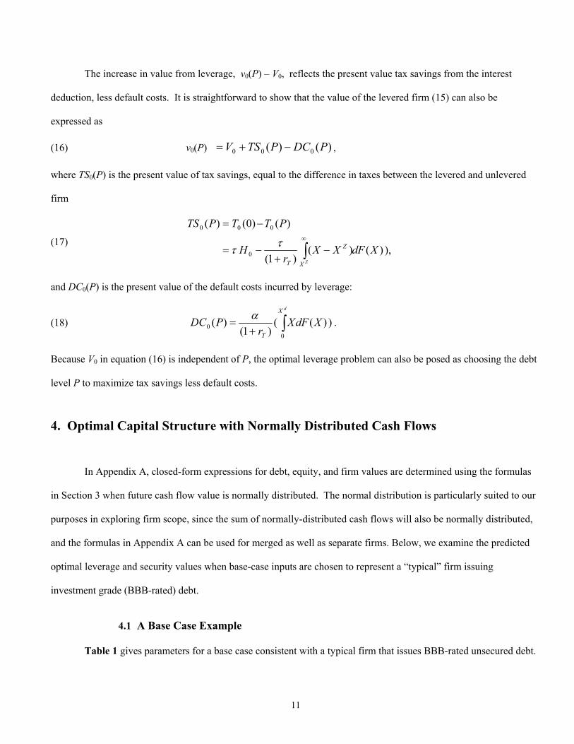
The increase in value from leverage, v0(P) – V0, reflects the present value tax savings from the interest

deduction, less default costs. It is straightforward to show that the value of the levered firm (15) can also be

expressed as

(16) v0(P) )()( 000 PDCPTSV −+= ,

where TS0(P) is the present value of tax savings, equal to the difference in taxes between the levered and unlevered

firm

(17) ),)()(

)1(

)()0()(

0

000

XdFXXr

H

PTTPTS

ZX

Z

T∫∞

−+

−=

−=

ττ

and DC0(P) is the present value of the default costs incurred by leverage:

(18) ))(()1(

)(0

0 XdFXr

PDCdX

T∫+

=α

.

Because V0 in equation (16) is independent of P, the optimal leverage problem can also be posed as choosing the debt

level P to maximize tax savings less default costs.

4. Optimal Capital Structure with Normally Distributed Cash Flows

In Appendix A, closed-form expressions for debt, equity, and firm values are determined using the formulas

in Section 3 when future cash flow value is normally distributed. The normal distribution is particularly suited to our

purposes in exploring firm scope, since the sum of normally-distributed cash flows will also be normally distributed,

and the formulas in Appendix A can be used for merged as well as separate firms. Below, we examine the predicted

optimal leverage and security values when base-case inputs are chosen to represent a “typical” firm issuing

investment grade (BBB-rated) debt.

4.1 A Base Case Example

Table 1 gives parameters for a base case consistent with a typical firm that issues BBB-rated unsecured debt.

12

The annual riskfree interest rate r = 5% approximates recent intermediate term Treasury note rates. The length of the

time period T is assumed to be 5 years.12 The capitalization factor is Z = (1 + r)T/((1 + r)T – 1) = 4.62.13 Expected

operational cash flow Mu = 127.6 is chosen such that its present value X0 = 100. Operational cash flow at the end of

5 years has standard deviation (Std) of 49.2, consistent with an annual standard deviation of cash flows equal to 22.0

(= 49.2/√5) if annual cash flows are additive and i.i.d.14 Henceforth we express volatility σ as an annual percent of

initial activity value X0, e.g. σ = 22% in the base case.

TABLE 1: BASE CASE PARAMETERS

Variables Symbols ValuesAnnual Riskfree Rate r 5.00%

Time Period/Debt Maturity (yrs) T 5.00T-period Riskfree Rate r T = (1 + r )T - 1 27.63%

Capitalization Factor Z = (1+r T )/r T 4.62

Unlevered Firm Variables

Expected Future Operational Cash Flow at T Mu 127.63Expected Operational Cash Flow Value (PV) X 0 = Mu / (1+r )T 100.00

Cash Flow Volatility at T Std 49.19Annualized Operational Cash Flow Volatility σ = Std/T 0.5 22.00

Tax Rate τ 20%Value of Unlevered Firm w/Limited Liability V 0 80.05

Value of Limited Liability L 0 0.057

The tax rate τ = 20% is chosen in conjunction with other parameters to generate a capitalized value of optimal

leverage (Z(v0* - V0)/V0) of 8.2 percent.15

12 This lies between Stohs and Maurer’s (1996) estimate for average debt maturity of 4.60 years for BBB-rated firms (based on data 1980-1989), and the Lehman Brothers Credit Investment Grade Index Average duration (5.75 as of 9/30/04). 13 For a discussion of capitalizing T-period flows and the factor Z, see Section 5.4 below. 14 Annualized operational cash-flow volatility σ of 22 (22% of X0) is based on Schaefer and Strebulaev (2004), who estimate asset volatility from equity volatility for firms with investment-grade debt over the period 1996-2002. This volatility also approximates the 23% asset volatility that Leland (2004) finds to match Moody’s observed default rates on long-term investment-grade debt over the period 1980-2000, using a structural model of debt.

13

Table 2 shows the optimal capital structure for a firm with base-case parameters. The default cost parameter

α = 23% generates a recovery rate of 49.3%, close to empirical estimates of recovery rates on senior debt.16 The

level of optimal debt P* is derived numerically. Given P* other values are computed from the closed-form solutions

in Appendix A.

TABLE 2: OPTIMAL CAPITAL STRUCTURE

Symbols ValuesDefault Costs α 23%

Optimal Zero-coupon Bond Principal P* 57.1Default Value X d 67.7

Breakeven Profit Level X Z 14.9Value of Optimal Debt D 0* 42.2

Optimal Leverage Ratio D 0*/v 0* 51.8%Annual Yield Spread of Debt (%) (P */D 0*)1/T - 1 - r 1.23%

Recovery Rate R 49.3%

Value of Optimal Equity E 0* 39.2Optimal Levered Firm Value v 0* = D 0*+E 0* 81.47

Tax Savings of Leverage (PV) TS 0 2.32Expected Default Costs (PV) DC 0 0.89Value of Optimal Leveraging v 0* - V 0 1.42

Capitalized Value of Optimal Leverage Z(v 0* - V 0)/V 0 8.21%

Optimal leverage is 51.8%. While somewhat greater than the leverage of an average BBB-rated firm, this

level may reflect Graham’s (2000) conclusion that firms are less leveraged than the optimal level.17 The base case

15 This premium for optimal leverage is consistent with estimates by Graham (2000) and Goldstein, Leland, and Ju (2000). If the corporate tax rate is τC and the marginal investor is taxable at rates τE on equity income and τP on interest income, then Miller (1977) derives an effective tax rate τ = 1 – (1-τC)(1-τE)/(1-τP). For post-1986 average personal and corporate tax rates, Graham (2003) shows that this would imply τ = 10%. However, several authors have found empirical evidence that τ may be considerably larger. Kemsley and Nissim (2002) estimate τ at almost 40%, and Engel, Erickson, and Maydew (1999) estimate 31%. 16 Elton et al. (2001) report BBB-rated debt average recovery rates of 49.4% for the period 1987-1996. Acharya et al. (2004) estimate average recovery of 49.7% for their sample of senior debt, 1982-1999. Direct evidence on α is mixed. Andrade and Kaplan (1998) suggest a range of default costs α from 10% to 23% of firm value at default, based on studies of firms undergoing highly leveraged takeovers (HLTs). However, firms subject to HLTs are likely to have lower-than-average default costs, since high leverage is more likely to be optimal for firms with this characteristic.

14

predicts a yield spread of 123 basis points on the debt.18 Thus the appropriately calibrated two-period model

generates yield spreads and an optimal capital structure that are highly plausible. In Section 6, this capital structure

model is used to explore the optimal scope of the firm.

Figure 1 plots optimal leverage as a function of volatility for two levels of default costs: the base case with

α = 23%, and with higher default costs α = 75%. Other parameters remain as in the base case. Note that when α =

23%, leverage first declines with volatility. But for annual volatility exceeding about 25%, leverage increases,

although not to the extreme levels found when volatility is low. Thus for moderate levels of default costs, two

different volatilities can generate the same optimal leverage ratio. However, when α = 75%. the optimal leverage is

monotonically decreasing to very high levels of volatility. This suggests that volatile firms with high default costs—

e.g. firms with substantial risky growth options—should avoid substantial leverage, consistent with Smith and Watts

(1992) and others.

Figure 2 plots the value of optimally-levered firm v* as a function of volatility σ when X0 is normalized to

100, with default costs α = 23% or α = 75% of X0. Value declines initially with risk, because higher volatility

lowers optimal leverage and leverage benefits. But as volatility increases, the value of the firm’s limited liability

shelter increases. We define σ L as the volatility at which v*(σ) reaches a minimum value.19 Although we do not

prove a general result, the optimal value function v*(σ) is strictly convex and U-shaped for all combinations of

parameters examined. The convexity of this schedule becomes important in studying the benefits of mergers between

firms with different volatilities, as shown in Section 6.

Finally, we note that v* is homogeneous of degree 1 in activity value X0 and σ , given α (as a percent of X).

Homogeneity requires the absence of a fixed component of default costs.

17 Schaefer and Strebulaev (2004) estimate the average leverage of a large sample of BBB-rated firms is 38% over the period 1996-2002. 18 Elton et al. (2001) report 5-year maturity BBB yield spreads of 120 bps for the period 1987-1996. 19 Observe that σ L depends upon other parameters including α.

15

5. Measures of Financial Synergies for Merged Activities

5.1 Measuring Financial Synergies

The problem of optimal firm scope is now considered. The decision is whether initially to incorporate (and

then leverage) two activities i = {1,2} separately, or to combine (“merge”) the activities in a single firm i = M and

leverage the merged firm.20 Additivity of operational cash flows implies that the future cash flows of the merged

firm equals the sum of the separate cash flows, i.e. XM = X1 + X2. This in turn implies from equation (1) that

(19) X0M = X01 + X02.

The financial benefit of merger ∆ is defined as the difference in value of the optimally-levered merged firm,

less the sum of the values of the optimally-levered separate firms:

(20) ∆ ≡ v0M (PM*) – v01(P1*) – v02(P2*),

where v0i (Pi) is given by equation (15) or (16), i = {1,2,M}, and Pi* is the debt principal that maximizes v0i (Pi). A

positive ∆ implies that merger increases total firm value, while a negative ∆ implies that separation increases value.

5.2 Identifying the Sources of Financial Synergies

From (20) and (16), financial synergies ∆ can be decomposed into three components:

(21) ∆ = ∆V0 + ∆TS - ∆DC,

where ∆V0 ≡ V0M – V01 – V02, ∆TS ≡ TS0M – TS01 – TS02, and ∆DC ≡ DC0M – DC01 – DC02.

The first component of financial synergies, ∆V0, is the change in unlevered firm value that results from

mergers. The other components are directly related to changes in financial structure: ∆TS, the change in value of tax

savings from optimal leveraging of the merged vs. separate firms; and ∆DC, the change in value of default costs.

Despite operational cash flow additivity, mergers can create value changes ∆V0 that are unrelated to

leverage effects. When tax rates are identical across firms (τ i = τ ), the change in unlevered firm values ∆V0 can be

written from (4) as 20 When firms are separately incorporated initially and later merged, or vice versa, the question of how previously-issued debt is retired (or assumed) becomes important. This is discussed in Section 7 below.

16

(22) ∆V0 = (1- τ)(H0M – H01 – H02)

= (1- τ)((X0M – X01 – X02) + (L0M(0) – L01(0) – L02(0) )) using (3)

= (1- τ) (L0M(0) – L01(0) – L02(0) ) using (19)

= SE,

where

(23) SE ≡ (1 – τ)(L0M(0) – L01(0) – L02(0)).

SE, the Sarig effect, is the (after-tax) difference in the value of limited liability to the merged firm compared to the

total value of limited liability to the separate firms. Sarig (1985) shows that SE is never positive, and is strictly

negative if operational cash flows have a positive probability of being negative and are less than perfectly correlated.

We shall sometimes refer to ∆V0 as the “Sarig effect.” 21

The second source of financial synergies from mergers, ∆TS, is the gain (or loss) in tax savings solely related

to the effects of optimal separate leverage versus merged leverage. Examples in Section 6 show that ∆TS can have

either sign. Even when debt principal increases after merger, a significantly lower debt credit spread may result in

lower total interest deductions, with a subsequent loss of expected tax savings. The final source of financial synergies

is the change in the value of default costs, ∆DC.

The last two terms may be combined into a single net “leverage effect” term, LE ≡ ∆TS – ∆DC. Thus an

alternative decomposition of merger benefits is

(24) ∆ = SE + LE.

In the cases studied below, the leverage effect can be positive or negative.

5.3 Scaled Measures of Synergies

21 If there are additional nondebt tax deductions K, the convexity of the tax schedule will be at K rather than zero, and the expression for ∆V0 will be more complex than equation (22). For sufficiently high K, the tax convexity effect can exceed the loss of separate limited liability and ∆V0 > 0. Of course, tax loss offsets would reduce the convexity of the tax schedule, and hence reduce the tax convexity effect.

17

We consider three ways in which financial synergies ∆ may be scaled. We adopt the convention that Firm 1

is the acquiring firm, and Firm 2 is the acquired or target firm.

Measure 1. ∆ / ( V01 + V 02 ). Measure 2. ∆ / v2 (P2*).

Measure 3. ∆ / E02(P2*).

Measure 1 expresses synergies as a percentage of the sum of the separate firms’ unlevered pre-merger

values.22 When ∆ < 0, Measure 1 is negative and reflects the benefits of separation.

Competition may induce an acquiring firm to bid an amount that reflects total synergies, including financial

synergies.23 If the target receives all the potential merger benefits, it will receive a percentage value premium of its

pre-merger value v2* given by Measure 2. Measure 2 is also useful in spin-offs or asset securitization, where its

negative, – ∆ / v2 (P2*), reflects the benefits of separation as a percent of the value of assets spun off (when

subsequently optimally leveraged).

Measure 3 is relevant when all financial benefits accrue to the stockholders of the target firm. It reflects the

percentage premium that the acquiring firm could pay for the target firm’s equity based on financial synergies alone.

Note that generally the absolute values of Measure 1 < Measure 2 < Measure 3.

5.4 Adjusting Benefit Measures For an Infinite Horizon

The measures of benefits introduced above reflect the length T of the single time period assumed. Shorter

time periods will generate smaller tax benefits (and usually lower bankruptcy costs). But since firms do not have

finite maturity, they can realize additional benefits in subsequent time periods with positive probability.

22 An alternative to Measure 1 is to express ∆ as a percentage of the sum of the optimally-levered separate firm values, i.e. ∆ / (v1* + v2*), or as a percentage of the optimally-levered merged firm value, i.e. ∆ / vM*. Since vi* as well as ∆ changes with leverage, these measures (in contrast to Measure 1) will not necessarily be monotonic in absolute benefits ∆. Note that Measures 2 and 3 below are non-monotonic, but are comparable to available statistics on the percentage merger gains for target firms. 23 Numerous studies (e.g. Andrade, Stafford, and Mitchell (2001)) suggest that acquiring firms realize little or no increases in their market value. Firms being acquired, however, realize substantial value premiums.

18

A complete solution to the multi-period problem is difficult in the normally-distributed future cash flow case,

and we do not attempt a fully dynamic modeling.24 Rather, we follow Modigliani and Miller (1958) and many others

by capitalizing the value of cash flows that occur over the single T-year period. Recall that the present value of a

perpetual stream of expected payments ∆ received at the end of each period of length T is PV(∆ ) = ∆ / rT, where rT

is the (constant) interest paid over a period of length T years. Risk neutrality implies that the appropriate interest rate

is the riskfree rate. The present value of these future payments, plus ∆ at t = 0, is ∆ / rT + ∆ = Z∆, where

Z = (1 + rT)/rT . 25 Equivalently, Z = (1 + r)T/((1 + r)T – 1) where r is the annual interest rate. Subsequent examples

scale Measures 1-3 by the factor Z.

Note that Z ∆ will preserve the ordering of ∆. Therefore the nature of our results is independent of Z. Z

serves only as a reasonable means for adjusting the net benefits derived for a period of T years to a long-term horizon.

6. How Large are Financial Synergies?

This section assumes activities’ cash flows are normally distributed. When the separate cash flows Xi are

jointly normally distributed (i = {1,2}) with means Mui, standard deviations Stdi, and correlation ρ, the merged

activity cash flow XM = X1 + X2 is normally distributed with

(25) Mu M = Mu 1 + Mu 2; Std M = (Std 12 + Std 2

2 + 2 ρ Std 1 Std 2)

0.5.

Whenever ρ < 1, the merger creates risk reduction due to diversification: Std M < Std 1 + Std 2. Defining the

annualized standard deviation of cash flow as σ i = Stdi / T0.5, observe that

(26) σ M (ρ) = (σ 12 + σ 2

2 + 2 ρ σ 1 σ 2)

0.5 24 In contrast, the multi-period case is quite straightforward to model when cash flows of firms follow a logarithmic random walk, resulting in lognormally-distributed future values (e.g., Leland 1994). However, a problem arises for studying mergers, as the sum of lognormally-distributed cash flows is not lognormally distributed. 25 A “stylized environment” that justifies capitalizing the gain is the following. An entrepreneur initially owns two activities with life T years. If the entrepreneur merges the activities, optimally leverages them, and immediately sells at a fair price to outside investors, she will realize a value ∆ greater than if the activities were separately incorporated, optimally leveraged, and then sold. The entrepreneur has a subsequent set of activities with identical characteristics available at time T, with life until time 2T, and so on. In addition to the gain ∆ at time t = 0, gains of ∆ can therefore be realized at times t = T, t = 2T, etc. The present value of this infinitely repeated set of incremental cash flows is Z∆, where Z= (1 + rT)/rT, and represents the infinite-horizon value of merging activities vs. separation.

19

is an increasing function of ρ for given σ 1 and σ 2, with σ M (1) = σ 1 + σ 2 and σ M (−1) = |σ 1 – σ 2 |. The

valuation and capital structure results from Section 4 are now applied to the measures developed in Section 5, to

determine the sign and magnitude of financial synergies.

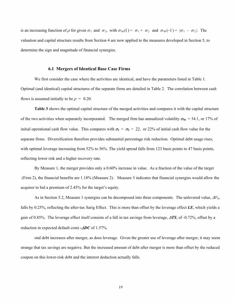
6.1 Mergers of Identical Base Case Firms

We first consider the case where the activities are identical, and have the parameters listed in Table 1.

Optimal (and identical) capital structures of the separate firms are detailed in Table 2. The correlation between cash

flows is assumed initially to be ρ = 0.20.

Table 3 shows the optimal capital structure of the merged activities and compares it with the capital structure

of the two activities when separately incorporated. The merged firm has annualized volatility σM = 34.1, or 17% of

initial operational cash flow value. This compares with σ1 = σ2 = 22, or 22% of initial cash flow value for the

separate firms. Diversification therefore provides substantial percentage risk reduction. Optimal debt usage rises,

with optimal leverage increasing from 52% to 56%. The yield spread falls from 123 basis points to 47 basis points,

reflecting lower risk and a higher recovery rate.

By Measure 1, the merger provides only a 0.60% increase in value. As a fraction of the value of the target

(Firm 2), the financial benefits are 1.18% (Measure 2). Measure 3 indicates that financial synergies would allow the

acquirer to bid a premium of 2.45% for the target’s equity.

As in Section 5.2, Measure 1 synergies can be decomposed into three components. The unlevered value, ∆V0,

falls by 0.25%, reflecting the after-tax Sarig Effect. This is more than offset by the leverage effect LE, which yields a

gain of 0.85%. The leverage effect itself consists of a fall in tax savings from leverage, ∆TS, of -0.72%, offset by a

reduction in expected default costs -∆DC of 1.57%.

otal debt increases after merger, as does leverage. Given the greater use of leverage after merger, it may seem

strange that tax savings are negative. But the increased amount of debt after merger is more than offset by the reduced

coupon on this lower-risk debt and the interest deduction actually falls.

20

TABLE 3: FINANCIAL EFFECTS OF MERGING FIRMS

Sum of Separate Merged FirmSymbols Firm Values Values Change

Value of Limited Firm Liability L 0 0.115 0.006 -0.11

Optimal Zero-coupon Bond Principal P* 114.27 117.42 3.15Default Value Xd 135.38 139.77 4.38

Value of Optimal Debt D 0* 84.47 89.40 4.94Optimal Leverage Ratio D 0*/v 0* 51.84% 54.80% 2.96%

Annual Yield Spread of Debt (%) (P */D 0*)1/T - 1 - r 1.23% 0.60% -0.63%Recovery Rate R 49.29% 56.48% 7.19%

Value of Optimal Equity E 0* 78.47 73.74 -4.73Optimal Levered Firm Value v 0* = D 0*+E 0* 162.94 163.15 0.21

Tax Savings of Leverage (PV) TS 4.63 4.39 -0.25 ∆ TSExpected Default Costs (PV) DC 1.79 1.25 -0.54 ∆ DC

Net Leverage Benefit TS - DC 2.85 3.14 0.30 SUMMARY OF BENEFITS

Change in Unlevered Firm Value ∆ V 0 -0.09 "Sarig Effect"Benefit to Leverage ∆ TS - ∆ DC 0.30 "Leverage Effect"

Net Benefit of Merger ∆ = ∆ V 0 + ∆ TS - ∆ DC 0.21Measure 1 Z ∆ / (V01 + V02) 0.60%Measure 2 Ζ ∆ / v2* 1.18%Measure 3 Ζ ∆ / E2* 2.45%

Financial synergies to identical firms merging in the base case are therefore positive but very modest.

Transactions fees to complete a merger would likely outweigh the benefits gained. This result is reassuring: it would

be surprising if our analysis suggested that two identical “average” firms should merge solely to realize financial

synergies. However, as the scenario diverges from the base case scenario and symmetric activities, situations arise

where financial synergies can be substantial. This is most pronounced where synergies are negative and provides a

rationale for many aspects of structured finance, as is seen in Section 7 below.

6.2 Comparative Statics: the Symmetric Case

Figure 3A shows how financial synergies change as the correlation of cash flows varies from 0 to 1. Not

surprisingly, increased correlation reduces all measures of merger benefits as diversification is less pronounced. Each

component of financial synergies is reduced but retains the same sign as correlation increases. When cash flows are

perfectly correlated there are zero financial synergies. Figure 3B changes (only) the annual volatilities of the

21

symmetric firms to 24% each. Now the Sarig effect becomes important. As correlation increases, the benefits of

leverage diminish and financial synergies become negative.

Figure 4 demonstrates the effect of changing (joint) volatility on merger benefits. While quite low volatilities

lead to greater Measure 1 and Measure 2 benefits, these decline as volatilities approach zero (and optimal leverage for

both separate and merged firms approaches 100 percent). Measure 3 benefits continue to increase as volatilities

approach zero, because equity values also approach zero as leverage increases.

Thus mergers of similar firms have greater financial synergies when correlation is low, and volatilities are

somewhat lower than average firm volatility. Financial synergies to merger also increase when default costs α rise

above average.26 In an extreme case with α = 100% (implying zero recovery on defaulted debt), merger synergies are

2.5 times as large as when α = 23%. Ceteris paribus, firms with high default costs will realize greater financial

synergies from merger, as diversification reduces the risks of incurring such costs.

Does target size matter? Figure 5A plots measures of financial synergies as a function of the size of the

target firm for base case parameters. The smaller the target firm (Firm 2) relative to the acquirer, the smaller are total

benefits by Measure 1. But as a proportion of the value of the target firm (Measure 2) or the value of the target firm’s

equity (Measure 3), there can be an optimal-sized target. The plot is nonlinear because the volatility of the merged

activity is a nonlinear function of the relative size of the two firms. Although Measure 1 rises monotonically with the

relative size of the target firm until it equals the acquirer’s size, Measures 2 and 3 are humped. An “ideal” target

would range between about 40% and 80% of the acquirer’s size. When volatility of both firms falls, so does the

optimal target size. Figure 5B examines the size effect for identical (but for size) firms with different base

parameters. The firms i = {1,2} each have volatility σ i = 15% and α i = 75%, and their returns are uncorrelated. In

this case the “ideal” target size is smaller, at less than 20% of the acquirer’s size.

How large can positive synergies realistically get when firms are symmetric? The parameters for Figure 5B

were chosen with this question in mind. When the target firm is 10 percent of the acquirer’s size, the financial

26 For low levels of α, the optimum capital structure may require 100% leverage. Except as noted, the (interior) leverage optimum is the global optimum in all examples below.

22

synergies represent a 8.2% value premium on the target firm’s value (Measure 2), and 14.6% of the target firm’s

equity value (Measure 3). 27

Negative synergies can be even larger. In the base case with annual volatility 40% of cash flow value for both

firms, Measure 2 is -18.8%, indicating the parent firm (Firm 1) could spin off Firm 2 and realize a value premium of

almost 20%. This advantage to separation primarily reflects the negative Sarig effect, but the leverage effect is

negative as well. 28

6.3 Comparative Statics: Asymmetric Volatility

We now vary the parameters of the target firm, when Firm 1 retains base case parameters. Figure 6 examines

the effect of changing the target firm’s volatility σ 2, keeping the acquirer’s annual volatility fixed at σ 1 = 22. The

measures of merger benefits are humped. Maximum financial synergies occur when Firm 2 has slightly lower

volatility. Financial synergies are negative when the target’s volatility is very different from the acquirer’s volatility.

Figure 7 decomposes the financial synergies of Measure 1 in Figure 3 into two components: that related to

the loss of separate limited liability (the after-tax Sarig effect), and that related to the net benefits (costs) of financial

structure, the leverage effect. When Firm 2 volatility is high, mergers become costly largely because of the Sarig

effect. A spin-off is desirable if the activities are already merged. When Firm 2 volatility is very low, the negative

leverage effect dominates. Spin-offs are desirable here because Firm 2 can benefit from high leverage, whereas the

optimal leverage and tax savings of the combined firm is considerably less. Section 7.1 below further explores this

rationale in the context of asset securitization.

27 Andrade, Mitchell, and Stafford (2001) estimate the median target firm was about 11.7% the size of the acquiring firm, based on a sample of mergers over the period 1973-1998. They also find that the 3-day abnormal returns to acquired firms is 16% of equity value (24% over a longer window that includes close of the merger). The return to acquiring firms is slightly negative but insignificantly different from zero, consistent with using Measure 3. The Measure 3 return here of 14.4% suggests that financial synergies have the potential to explain a substantial proportion of realized merger gains in specialized situations. 28 In very high-risk cases, courts may disallow spinoffs if found to be undertaken principally to avoid future liabilities. When Firm 2 volatility is 40%, the risk-neutral probability of negative cash flow is about 7.7 percent at the end of 5 years. Assuming a 6% annual risk premium for operational cash flow value (implying an expected annual return on value of 11%), the actual probability of negative terminal cash flow is 3.0 percent.

23

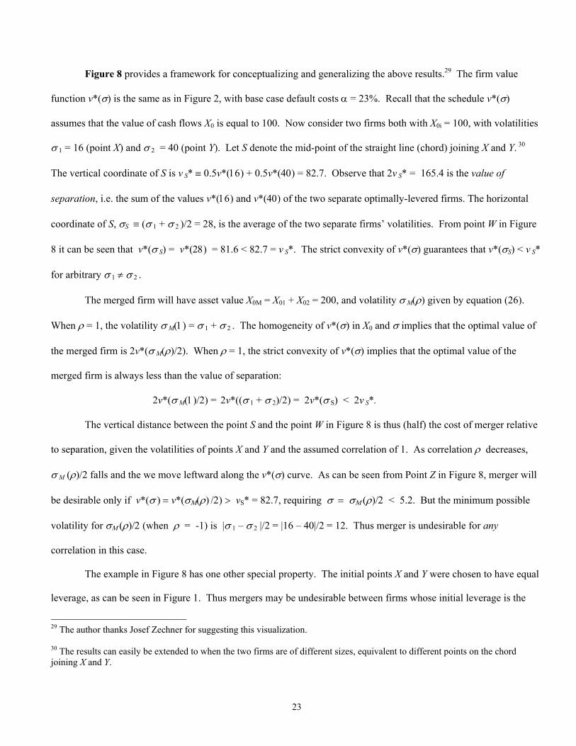
Figure 8 provides a framework for conceptualizing and generalizing the above results.29 The firm value

function v*(σ) is the same as in Figure 2, with base case default costs α = 23%. Recall that the schedule v*(σ)

assumes that the value of cash flows X0 is equal to 100. Now consider two firms both with X0i = 100, with volatilities

σ 1 = 16 (point X) and σ 2 = 40 (point Y). Let S denote the mid-point of the straight line (chord) joining X and Y. 30

The vertical coordinate of S is v S* ≡ 0.5v*(16) + 0.5v*(40) = 82.7. Observe that 2v S* = 165.4 is the value of

separation, i.e. the sum of the values v*(16) and v*(40) of the two separate optimally-levered firms. The horizontal

coordinate of S, σS ≡ (σ 1 + σ 2 )/2 = 28, is the average of the two separate firms’ volatilities. From point W in Figure

8 it can be seen that v*(σ S) = v*(28) = 81.6 < 82.7 = v S*. The strict convexity of v*(σ) guarantees that v*(σS) < v S*

for arbitrary σ 1 ≠ σ 2 .

The merged firm will have asset value X0M = X01 + X02 = 200, and volatility σ M(ρ) given by equation (26).

When ρ = 1, the volatility σ M(1) = σ 1 + σ 2 . The homogeneity of v*(σ) in X0 and σ implies that the optimal value of

the merged firm is 2v*(σ M(ρ)/2). When ρ = 1, the strict convexity of v*(σ) implies that the optimal value of the

merged firm is always less than the value of separation:

2v*(σ M(1)/2) = 2v*((σ 1 + σ 2)/2) = 2v*(σ S) < 2v S*.

The vertical distance between the point S and the point W in Figure 8 is thus (half) the cost of merger relative

to separation, given the volatilities of points X and Y and the assumed correlation of 1. As correlation ρ decreases,

σ M (ρ)/2 falls and the we move leftward along the v*(σ) curve. As can be seen from Point Z in Figure 8, merger will

be desirable only if v*(σ ) = v*(σΜ(ρ) /2) > vS* = 82.7, requiring σ = σΜ (ρ)/2 < 5.2. But the minimum possible

volatility for σΜ (ρ)/2 (when ρ = -1) is |σ 1 – σ 2 |/2 = |16 – 40|/2 = 12. Thus merger is undesirable for any

correlation in this case.

The example in Figure 8 has one other special property. The initial points X and Y were chosen to have equal

leverage, as can be seen in Figure 1. Thus mergers may be undesirable between firms whose initial leverage is the

29 The author thanks Josef Zechner for suggesting this visualization. 30 The results can easily be extended to when the two firms are of different sizes, equivalent to different points on the chord joining X and Y.

24

same, when the firms are identical except for volatility. Presuming that mergers are always beneficial when separate

firms have equal leverage is incorrect.31

While the preceding analysis has considered a single example, similar analysis can be used to explore

arbitrary points X and Y on v*(σ). The following propositions offer general results for firms when volatilities strictly

differ. The propositions assume that cash flows are normally distributed and that v*(σ) is strictly convex.32 Recall σL

is the volatility at which v*(σ) reaches a minimum (σL ≤ ∞), and σ M (ρ) is given by equation (26).

Proposition 1. Mergers of firms with differing volatilities will be undesirable for activities with high

correlations.

More formally, Proposition 1 can be stated: For any given volatilities σ1 ≠ σ2, there exists an interval NO =

(ρ +, 1] of positive measure such that merger will be undesirable when cash flow correlation ρ lies within NO.

Proofs of all Propositions are provided in Appendix B.

Proposition 2. Mergers of firms with differing volatilities will be desirable for activities with low

correlations if σ 1 , σ 2 < σ L .

More formally: The exists an interval YES = [– 1, ρ # ) of positive measure such that mergers will always be

desirable when cash flow correlation ρ lies within YES, and σ 1 , σ 2 < σ L .

Proposition 3. Mergers of firms with differing volatilities will be undesirable for all correlations

if and only if the total value of the separate firms is greater than or equal to the merged value

with volatility |σ 1 – σ 2 |.

31 The author thanks the referee for clarifying this point. Note in Figure 2 that when default costs are high (α = 75%), leverage will be monotonically decreasing over the range of relevant firm volatilities. In this case, differences in volatilities will also be reflected by differences in leverage. 32 The lack of a closed form expression for optimal leverage has precluded a proof of the convexity of v*(σ). However, all examples considered have exhibited a strictly convex, U-shaped v*(σ) schedule with σL < ∞.

25

The following propositions offer more general conclusions about merger benefits when firms have identical

volatilities σ 1 = σ 2 = σ0 (e.g. when points X and Y in Figure 8 coincide):

Proposition 4. Mergers of firms with identical volatilities σ 1 = σ 2 = σ 0 < σ L will be desirable

for all correlations ρ < 1.

Proposition 5. Mergers of firms with identical volatilities σ 1 = σ 2 = σ 0 > σ L will be undesirable

for high correlations (in the limiting case of perfect correlation, mergers will be weakly

undesirable).

Collectively, these propositions show that low correlation favors mergers. Proposition 4 indicates that when

volatilities are moderate (< σ L ) and firms are identical, mergers are always beneficial. This observation generalizes

the results observed in Figure 3A, noting (from Figure 1) that the base case volatility is slightly less than σ L . When

volatilities differ, or are identical but large (> σ L ), Propositions 1 and 5 indicate that separation is desirable at high

correlations. Proposition 5 generalizes the results observed in Figure 3B. When volatilities differ greatly, Proposition

3 shows that separation may be preferred for any correlation. This generalizes the example in Figure 8, where merger

between firms with volatilities 16% and 40% would never be beneficial.

6.4 Comparative Statics: Asymmetric Default Costs

Figure 9 charts the value of merger between two firms identical except for default costs. The default costs

of Firm 1 remain at the base case (α1 = 23%), while default costs α2 of Firm 2 vary. The merged firm is

presumed to have a default cost equal to the asset-value weighted default costs of the separate firms.

As with differential volatility in Figure 6, the benefits function is humped and becomes negative

when the costs are substantially different.33 Large differences in default costs favor separation. In contrast

with Figure 2, leverage ratios are strictly monotonic and decreasing in default costs. Thus firms with

33 We use correlation ρ = 0.50 in Figure 9 to illustrate that benefits can be negative both for low and high default costs α2 of Firm 2. With correlation 0.20, benefits shift upward. They are still negative for low α2, but remain positive as α2 exceeds 0.23.

26

different leverage ratios will be more likely to benefit from separation, when default costs are the source of

the leverage differences.

6.5 A Specific Counter-Example to Lewellen

Lewellen’s (1971) contention that financial synergies are always positive did not explicitly contemplate

negative future cash flows and the resulting Sarig effect. Absent negative future cash flows, might Lewellen’s

conjecture be correct? While the previous results suggest it is not, we show here a specific counter-example.

When cash flow volatilities are 15% or less, the probability of a negative cash flow in the base case is less

than 0.07% and the Sarig effect is negligible. Consider the base case but with Firm 1 volatility 15%, Firm 2 volatility

5%, and correlation 0.70. Then the financial benefits to merger are negative: ∆ = – 0.073. Decomposition of

benefits gives ∆V0 = (1 - τ)SE = 0.000 (as expected), tax savings ∆TS = -0.153, and default cost change ∆DC = -

0.081. Thus the leverage effect LE = – 0.073, and is entirely responsible for the negative financial synergies.

As a general rule of thumb, our examples suggest that mergers are beneficial (costly) if total debt value

increases (decreases) after merger. This holds true in both symmetric and asymmetric cases, when either volatility or

default costs are changing. Thus our predictions of situations in which mergers will be beneficial largely coincides

with situations in which the optimal post-merger debt will exceed the total optimal debt of the separate firms. This is

true in the counter-example above: debt value when firms are separate is 112.4 vs. 110.4 when merged.

6.6 Hedging and Mergers

The above results suggest that a link exists between hedging and the desirability of mergers. If activities’

volatilities can be altered by hedging, relative volatilities can be altered. Mergers that were previously desirable can

become undesirable, and vice-versa. From Figure 6, if Firm 2 can reduce its volatility from 30% to 20% by hedging,

merger now becomes desirable.34 If Firm 1 can reduce its volatility by hedging to 5% when Firm 2 has volatility

34 For the parallel between hedging and our analysis to be precise, it must be the case that hedges are fairly priced, that the distribution of cash flows will continue to be normally distributed (though with lower volatility), and that hedging will not affect the correlation between the activities.

27

22%, merger no longer is desirable. Whether the financial synergies to merger could be gained at a lower cost by

hedging is a question beyond the scope of this paper, but deserves further attention.

7. Spin-offs and Structured Finance

Spin-offs are reverse mergers: two previously-combined activities are separated into distinct corporations.

These corporations then leverage themselves individually. “Structured finance” is another means to separate an

activity from the originating or sponsoring organization. Asset securitization and project finance are examples of

structured finance. Assets generating cash flows are placed in a bankruptcy-remote (and off-balance sheet) SPE or

corporation formed specifically to hold those assets. 35 The SPE raises funds to compensate the sponsor by the sale of

securities collateralized by the activity’s cash flows.36 Both debt (often in tranches with differing seniority) and

equity (often termed the “residual tranche”) are typically issued by the SPE. A bankruptcy-remote SPE with limited-

recourse financing has the key features of a separate firm from our analytical perspective.37

Structured finance has boomed in recent years. Financial and industrial firms have transferred trillions of

dollars of mortgages, commercial loans, accounts receivables, power plants, motorway rights, and other cash flow

sources to special purpose entities. This raises the question: How does structured finance create value? It is claimed

beneficial both for activities with low-risk cash flows (e.g., mortgages) and activities with high-risk cash flows (e.g.,

major investment projects). It is sometimes argued vaguely that both spin-offs and structured finance “unlock asset

value.” But little formal analysis has examined the validity of such claims.38 Structured finance at first sight simply

35 We focus on “qualifying” SPEs, which are “demonstratively distinct” from the sponsor (see Gorton and Souleles (2005)). If the SPE is not demonstrably distinct, the SPE will fail to be a qualifying SPE under FAS 140. That in turn means that the transfer of assets to the SPE will not qualify as a “true sale” and that the SPE’s debt must be recognized on the sponsor’s balance sheet. 36 “True-sale” (cash) structured finance methods are based on sale of the assets to an SPE and primarily serve funding purposes. Synthetic methods involve portfolio swaps to transfer the risk to an SPE. We focus on true sale. 37 Our analysis presumes that the sponsoring firm does not guarantee the SPE debt. Explicit guarantees contradict the notion that the SPE is “demonstrably distinct” from the sponsor, with the negative consequences noted in footnote 37. Gorton and Souleles (2005) argue that there may nonetheless be implicit guarantees between SPE and sponsor. 38 An exception is Chemmanur and John (1996), who examine several of the issues considered here. But their focus is not on purely financial synergies, but rather on operational synergies resulting from differential managerial abilities across projects, and different benefits of control. Flannery et al. (1993) consider operational synergies related to underinvestment.

28

appears to carve up a given cash flow “pie”, and the original Modigliani-Miller argument implies that this should not

affect total value. Securitization has been justified by the assertion that separate, low volatility assets can attract lower

cost financing. But the residual assets will have higher volatility and higher financing cost, so this is not convincing a

priori. Gorton and Souleles (2005) argue that SPEs exist to avoid bankruptcy costs. Other reasons cited for structured

finance, which are not explored here, include the issuance of multiple debt classes (“tranching”), relaxation

of capital constraints (for financial institutions), and reduced informational asymmetry and agency costs.39

In the subsections below, we show that our model provides a clear rationale for structured finance based on

purely financial synergies. We can identify with precision the sources of these synergies, and put meaning in the

vague claims that structured finance can “unlock asset value.” The theory explains the use of these techniques for

both low-risk and high-risk assets.

7.1 Asset Securitization

Securitized assets typically have contractual cash flows with low volatility and utilize high leverage. As an

example of asset securitization, we use base case parameters to describe the originating firm prior to securitization.

While the typical SPE may issue multiple tranches of debt, we assume a single (senior) class of debt, plus equity.40

The originating firm is presumed to retain no equity in the SPE, and to distribute the funds received for the transferred

assets to shareholders.41

Table 5 outlines the parameters and results for our example. The securitized assets have low annual cash

flow volatility (4% of asset value), similar default costs (α2 = 23%, later reduced), and a correlation with the sponsor’s

other cash flows of 0.50. The firm before securitization is viewed as the merged firm (having parameters equal to 39 See, for example, DeMarzo (2005), Esty (2003), Greenbaum and Thakor (1987), Lockwood, Rutherford, and Herrera (1996), Oldfield (1997), and Rosenthal and Ocampo (1988). Oldfield (1998) and DeMarzo (2005) attribute tranching to price discrimination and information asymmetries, respectively. 40 Some asset securitizations offer a single-class participation only, and are termed “pass through” structures. More complex SPEs issue multiple securities (we consider one debt tranche and one equity tranche) and are termed “pay through” structures. See Oldfield (2000). Cash flow allocations to tranches when cash flow is insufficient to meet expected debt payments are contractually pre-determined when the SPE is formed, and formal default never occurs. 41 Originating banks typically retain no equity in current asset securitizations. If funds are not paid out to shareholders but retained as cash, the problem becomes one of optimal dividend policy and the benefit depends on personal vs. corporate tax rates. We do not address such issues here.

29

those assumed in Table 1). After securitization, the firm is split: “Firm 2” is the SPE that receives the cash flows of

the securitized assets; “Firm 1” receives all other cash flows and represents the sponsoring firm after securitization.

The value of the assets securitized is one-quarter of firm value before securitization. Given these assumptions, the

residual cash flow of the sponsor has annual volatility σ2 = 28.6%.

TABLE 5: ASSET SECURITIZATION EXAMPLE

Firm Before After Securitization:Symbols Securitization SPE Firm Change

Value of Operational Cash Flows X 0 100 25 75 0Value of Unlevered Firm V 0 80.05 20.00 60.26 0.21 −∆ V 0

Value of Limited Firm Liability L 0 0.06 0.000 0.33 0.27Annual Volatility (as % of X 0) σ 22.0% 4.0% 28.6%

Optimal Zero-coupon Bond Principal P* 57.13 21.96 45.74 10.57Value of Optimal Debt D 0* 42.24 17.18 31.85 6.80

Optimal Leverage Ratio D 0*/v 0* 51.8% 82.9% 51.9%Annual Yield Spread of Debt (%) (P */D 0*)1/T - 1 - r 1.23% 0.04% 2.51%

Recovery Rate R 49.3% 70.6% 41.7%

Optimal Levered Firm Value v 0* = D 0*+E 0* 81.47 20.72 61.35 0.61 −∆

Tax Savings of Leverage (PV) TS 2.32 0.75 2.11 0.54 −∆ TSExpected Default Costs (PV) DC 1.01 0.03 0.89 -0.14 −∆ DC

SUMMARY OF BENEFITS TO ASSET SECURITIZATION

- ∆ 0.61(minus) Measure 1 -Z ∆ / (V 01 + V 02) 3.51%(minus) Measure 2 −Ζ ∆ / v 02* 13.57%

Securitization of the base case firm’s assets generates an almost 14% increase in value relative to the assets

secured (the negative of Measure 2). This is a substantial value increase from a purely financial change. The optimal

leverage for the securitized assets rises to 83%. (This would equate to the size of the SPE’s “senior tranche” debt).

The debt has minimal risk of default and a very low credit spread, consistent with the observed high credit ratings on

senior tranche debt. Note that separation has led to a substantial increase in the total amount of debt that is optimal.

These results justify some of the informal arguments for asset securitization cited above. Securitization

permits the use of very high leverage on the subset of low-risk assets. About 66 percent (0.40/0.61) of the benefits

come from the leverage effect, reflecting an increase in debt of about 15%. The remaining 34 percent of securitization

benefits come from the (after-tax) Sarig effect, reflecting the increased value of the limited liability shelters for the

sponsor after securitization.

30

Securitization is even more desirable when the sponsoring firm is riskier. If the volatility of the sponsoring

firm before securitization is 25 rather than 22, benefits rise from 14% to 20% of secured asset value. Gorton and

Souleles (2005) present preliminary empirical results that suggest the riskiest banks (with debt ratings single B) are

the most likely to securitize credit card debt.

Gorton and Souleles (2005) further argue that the primary benefit of asset securitization is the low bankruptcy

(default) costs associated with the SPE structure. This contention can be directly addressed with our model. For

example, reducing the SPE’s default costs to 5% from 23% raises its optimal leverage from 83% to 88%, but the

advantage of securitization rises by only a modest amount, to 14.4% from 13.6%.42 The importance of lower default

costs seems relatively small in the example considered.

7.2 Separate Financing of High-Risk Projects

Large and risky investment projects can be internally financed by a firm, or financed separately as a spin-off

or through project finance. The formation of a separate firm or special purpose entity ensures that debt financing for

the project has recourse only to the project’s cash flows and assets.43 Commonly-cited justifications for separation

include greater total financing ability, cheaper financing for assets that remain in the firm, and preserving core firm

assets from bankruptcy risk. Berkovitch and Kim (1990) and Esty (2003) also mention the possible benefits of project

finance in reducing the opportunity costs of underinvestment in large and risky projects. These benefits would be

additional to the purely financial synergies that we consider here.

Our model provides insight into the decision. From Figure 6, it can be seen that separate financing benefits

(the negative of merger benefits) increase as the annual volatility of Firm 2 (“the investment project”) rises above the

volatility of Firm 1 (“the parent”). If the project is of equal size to the parent, and has annual volatility 50%, the

42 The optimal leverage of 87.7% is a global optimum within leverage ranges of 0% - 99.7%. However, by issuing an enormous amount of highly risky debt (driving leverage to 100% and virtually guaranteeing default), the value can be made higher since the interest deduction will eliminate taxes for virtually any level of X (i.e., XZ is very large), and default costs are modest. Since such risky debt is never observed, and the interest deduction would almost surely be disallowed, we ignore this corner solution. 43 Esty (2002, 2003) provides details on project financing. Our approach assumes that the parent firm retains no equity risk in the project, which is often the case with spinoffs but unusual with project finance. The analysis is more complex if the originating firm retains equity in the SPE: The equity of the originating firm becomes an option (due to the nature of equity) on a value that includes an option on another asset ( SPE equity). We are unaware of closed-form solutions to this problem, although preliminary numerical analysis suggests that the nature of our results will not be significantly changed.

31

benefits of separate financing to the parent firm represent almost 24% of project value. (If the project is half the size

of the parent firm, benefits rise to over 27% of project value). Approximately eighty percent of the value increase

comes from the additional limited liability shelter provided by separate financing, with the remainder coming from the

leverage effect. Compared with internal financing, the use of separate financing allows greater additional debt

financing (59% of project value vs. 52%), and keeps the credit spread of the parent firm at 123 bps (vs. 264 bps if the

Parent firm uses internal finance).

The model predicts that firms and projects with mutually high volatilities benefit from separate financing,

reflecting the Sarig effect. The leverage effect will be more pronounced when the volatilities of the parent firm and

investment project differ significantly. In cases where project finance is used for lower-risk activities (e.g. cash flows

from toll highway revenues), the analysis of Section 7.1 pertains.

8. Who Realizes the Financial Benefits of Mergers and Spin-offs?

If equity holders are to capture the entire financial synergies derived above, bondholders must not participate

in gains or losses. This poses no problem for start-up firms, where there is no initial debt. The entrepreneur decides

whether to incorporate activities jointly or separately, and subsequently levers the firm(s) optimally by issuing debt at

a price that fairly reflects risks. If the separate firms have extant debt that is callable at par, or otherwise can be retired

at a price that reflects pre-merger risks, again the separate firms’ bondholders will not participate in windfall gains

from a merger.

As suggested by Higgins and Schall (1977), Kim and McConnell (1977) and Stapleton (1982), potential

problems arise when the extant debts of the separate firms are noncallable and are assumed by the post-merger firm.44

Transfer of value to bondholders can lead to value-enhancing mergers being rejected by shareholders. This

inefficiency is similar to the “debt overhang” problem discussed in Myers (1977), which also can prevent a value-

improving investment decision by the firm. Although Higgins and Schall et al. did not have a full model of capital

structure, we can show that their concerns are indeed warranted. 44 These authors consider value transfers to bondholders when the merged firm assumes the debt of the separate firms but does not issue or retire additional debt. They do not explicitly consider optimal financial structure.

32

In the base case of Table 3, the value of the outstanding bonds at the time of merger would rise by 3.08 after

the merger, reflecting their lower risk. This increase in value is far greater the benefits ∆ = 0.21 resulting from the

merger itself. Shareholders will suffer a substantial loss of value from merger in this case. In the more favorable

merger environment when firms have 15% volatility, merger benefits of ∆ = 0.93 will be substantially reduced (but

not eliminated) to shareholders by an increase in extant bond value of 0.60. These results are generally consistent

with the findings of Mansi and Reeb (2002), who conclude that although the value of equity in conglomerate mergers

drops, there is a significant increase in the value of debt above par (book value). They find that the net change in total

value is insignificantly different from zero.

The results also underscore an important reason for firms to issue callable debt. Such debt enables

corporations to reduce or eliminate windfall gains to bondholders. Windfall gains can also be reduced when the firm

uses short-term debt. Subsequent debt rollovers will carry an interest rate that reflects post-merger risks and

overpayment of interest to extant bondholders will occur only for a short time. In the base case with debt with

maturity two years (rather than five years), extant debt value increases only by 0.56 compared with 3.08. However,

firms have lower gains to leverage when short term debt is used. The capitalized gains to optimal leverage with a two

year rollover horizon are 7.5% of unlevered value, versus 8.2% when five year debt is used.

Spin-offs or project finance can cause an opposite problem. Extant bond values may fall after separation.45

Covenants can enable bondholders to extract compensation, perhaps through an option to immediately redeem the

bonds at face value. When such protective covenants do not exist, value-diminishing spin-offs may be profitable for

shareholders.

9. Conclusion

We analyze the purely financial synergies that result from combining vs. separating multiple activities. To

permit focusing on financial effects alone, the operational cash flows of activities are assumed to be additive and

therefore nonsynergistic. A simple two-period model generates the optimal capital structure for separate or combined 45 The 1993 Marriott spinoff is a classic example. See R. Parrino (1997). In the example in Table 5, extant bondholders will lose almost 4% of bond value (even assuming that the amount of principal retired is bought back at pre-spinoff market value).

33

activities. When cash flows are jointly normally distributed, closed form valuation formulas determine debt and

equity values given debt principal. Numerical optimization finds the optimal amount debt.

The model then compares optimal values when activities are separately incorporated, or merged into a single

firm. A complex interaction of activities’ cash flow risks, correlation, tax rates, default costs, and relative size

determines the value-maximizing scope of the firm. Despite this complexity, some general principles can be

ascertained.

There are two sources of purely financial benefits (or costs) from merger. The first source, the Sarig effect, is

always nonpositive and hence favors separation. It reflects the loss of separate firm limited liability shelters when the

activities are combined. It is unrelated to leverage. The Sarig effect is strictly negative when operational cash flows

can be negative and is more significant when operational cash flow volatilities are high and correlation is low.

The second source of financial synergies is the leverage effect. It reflects the benefits of leverage when

activities are jointly versus separately incorporated, and can be expressed as (i) merged vs. separate tax savings from

leverage less (ii) merged vs. separate default costs. Contrary to Lewellen’s (1971) contention, the leverage effect can

have either sign. Combining activities into a single firm offers the advantage of risk-reduction from diversification.

But keeping activities separate offers the advantage of optimizing the separate capital structures. As a general rule of

thumb, the leverage effect is positive (negative) when the optimally-levered merged firm has greater (lesser) debt

value D0 than the sum of the separate optimally-levered debts.

The theory generates several testable hypotheses. Ceteris paribus, financial synergies from mergers are

greater when correlations are low, and volatilities are low and similar. Jointly high default costs also make mergers

more desirable, reflecting an increased value from risk-reduction through diversification. Substantial differences in

activities’ volatilities or default costs favor separation. Consistent with this hypothesis, Gorton and Souleles (2005)

find riskier banks are more likely to securitize low-risk assets. A further finding is that mergers with positive

financial synergies will have optimal debt value that exceeds total optimal debt value before merger.

How significant are purely financial synergies? In many cases, examples calibrated to empirical data suggest

that financial synergies are insufficient to justify mergers by themselves. But they can become important in

specialized circumstances.

34

The argument that purely financial synergies can justify separation is much stronger. When the volatilities are

jointly high, or are quite different, the benefits to separation are significant. The theory provides a strong rationale for

the existence of structured finance, including asset securitization and separate large project financing.

Finally, our results have implications for empirical work that examines the sources of merger gains or predicts

merger activity. Aspects of firms’ cash flows which can create substantial financial synergies, including correlation,

difference in volatilities, and difference in default costs, should be included as possible explanatory variables.

35

References Andrade, G., and Kaplan S. (1998), “How Costly is Financial (Not Economic) Distress? Evidence from Highly Leveraged Transactions that Became Distressed” Journal of Finance 53, 1443-94. Andrade, G., Mitchell M., and Stafford E. (2001), “New Evidence and Perspective on Mergers”, Journal of Economic Perspectives 15, 103-120. Aron, D. (1988), “Ability, Moral Hazard, Firm Size and Diversification,” RAND Journal of Economics 19, 72-87. Baron, D. (1975), “Firm Valuation, Corporate Taxes, and Default Risk,” Journal of Finance 30, 1251-1264. Berger, P., and Ofek, E. (1995), “Diversification’s Effect on Firm Value,” Journal of Financial Economics 37, 39- 65. Berkovitch, E., and Kim, E.H. (1990), “Financial Contracting and Leveraged Induced Over- and Under-Investment Incentives,” Journal of Finance 65, 765-794. Campa, J-M, and Kedia, S. (2002), “Explaining the Diversification Discount,” Journal of Finance 57, 1731-1762. Chemla, G. (2005), “Hold-Up, Stakeholders, and Take Over Threats,” Journal of Financial Intermediation, forthcoming. Chemmanur T., and John K. (1996), “Optimal Incorporation, Structure of Debt Contracts, and Limited-Recourse Project Financing'”, Journal of Financial Intermediation 5, 372-408. Coase, R. (1937), “The Nature of the Firm,” Economica 4, 386-405. DeAngelo, H., and Masulis, R. (1980), “Optimal Capital Structure Under Corporate and Personal Taxes”, Journal of Financial Economics 8, 3-29.

DeMarzo, P. (2005), "The Pooling and Tranching of Securities," forthcoming, Review of Financial Studies.

Elton, E., Gruber, M., Agarwal, D., and Mann, C. (2001), “Explaining the Rate Spread on Corporate Bonds,” Journal of Finance 56, 247-277.

Engel, E. M. Erickson, and E. Maydew, “Debt-Equity Hybrid Securities,” Journal of Accounting Research, 37, 249-274. Esty, B. (2002), “An overview of the project finance market—2002 Update,” Harvard Business School Case Study 202-105. Esty, B. (2003), “The Economic Motivation for Using Project Finance,” Harvard Business School mimeo, February. Esty, B. (2004) “Why Study Large Projects? An Introduction to Research on Project Finance,” European Financial Management 10, 213-224. Faure-Grimaud, A., and Inderst, R. (2004), “Conglomerate Entrenchment Under Optimal Financial Contracting,” forthcoming, American Economic Review.

36

Flannery M., Houston J., and Venkataraman S. (1993), “Financing Multiple Investment Projects”, Financial Management 22, 161-172. Gorton, G., and Souleles, N. (2005), “Special Purpose Vehicles and Securitization,” Working Paper 11190, National Bureau of Economic Research, March. Graham, John R. (2000), “How Big Are the Tax Benefits of Debt?”, Journal of Finance 55, 1901-1941. Graham, J., Lemmon, M., and Wolf, J. (2002), “Does Corporate Diversification Destroy Value?” Journal of Finance 57, 695-720. Grossman, S., and Hart, O. (1986), “The Costs and Benefits of Ownership: A Theory of Vertical and Lateral Integration,” Journal of Political Economy 94, 691-719. Harris, M., Kriebel, C., and Raviv, A. (1982), “Asymmetric Information, Incentives, and Intrafirm Resource Allocation,” Management Science 28, 604-620. Hart O., and Moore J. (1990), “Property Rights and the Nature of the Firm”, Journal of Political Economy 98, 1119-1158. Higgins, R., and Schall, L. (1975), “Corporate Bankruptcy and Conglomerate Merger,” Journal of Finance 30, 93- 113. Holmstrom, B., and Roberts, J. (1998), “The Boundaries of the Firm Revisited,” Journal of Economic Perspectives 12, 73-94. Jensen, M. (1986), “Agency Costs of Free Cash Flow, Corporate Finance, and Takeovers,” American Economic Review 76, 323-329. John T. (1993), “Optimality of Spin-Offs and Allocation of Debt'”, Journal of Financial and Quantitative Analysis 28, 139-160. John K., and John T. (1991), `”Optimality of Project Financing: Theory and Empirical Implications in Finance and Accounting”, Review of Quantitative Finance and Accounting 1, 51-74. Kale, J., Noe, T., and Ramirez, G. (1991), “The Evidence of Business Risk on Corporate Capital Structure: Theory and Evidence, Journal of Finance 46, 1693-1715. Kemsley, D., and Nissim, D. (2002), “Valuation of the Debt Tax Shield,” Journal of Finance 57, 2045-2073. Kim H., and McConnell J. (1977), “Corporate Mergers and the Co-Insurance of Corporate Debt”, Journal of Finance 32, 349-365. Kleimeier S., and Megginson W. (1999), “An Empirical Analysis of Limited Recourse Project Finance,” Working Paper, Michael Price College of Business, University of Oklahoma. Lang, L., and Stulz, R. (1994), “Tobin’s q, Corporate Diversification, and Firm Performance,” Journal of Political Economy 102, 1248-1280. Leland H. (1994), "Corporate Debt Value, Bond Covenants, and Optimal Capital Structure," Journal of Finance 49, 1213-1252.

37

Leland, H. (2004) “Predictions of Default Probabilities in Structural Models of Debt,” Journal of Investment Management 2, 5-20. Levy, H., and Sarnat, M. (1970), “Diversification, Portfolio Analysis, and the Uneasy Case for Conglomerate Mergers,” Journal of Finance 25, 795-802. Lewellen, W. (1971), `”A Pure Financial Rationale for the Conglomerate Mergers'”, Journal of Finance 26, 521-537. Li D., and Li S. (1996), “A Theory of Corporate Scope and Financial Structure”, Journal of Finance 51, 691-709. Lockwood, L., Rutherford, R., and Herrera, M. (1996), “Wealth Effects of Asset Securitization,” Journal of Banking and Finance 20, 151-164. Maksimovic, V., and Philips, G. (2001), “Do Conglomerate Firms Allocate Resources Efficiently?” Journal of Finance 56. Mansi, S., and Reeb, D. (2002), “Corporate Diversification: What Gets Discounted?” Journal of Finance 57, 2167-2183. Martin, J., and Sayrak, A. (2003), “Corporate Diversification and Shareholder Value: A Survey of Recent Literature,” Journal of Corporate Finance 9, 37-57.

Merton, R., 1974, “On the pricing of corporate debt: The risk structure of interest rates,” Journal of Finance, 29, 449-470.

Miller, M. (1977), “Debt and Taxes”, Journal of Finance 32, 261-275. Modigliani, F., and Miller, M. (1958), “The Cost of Capital, Corporation Finance and the Theory of Investment”, American Economic Review 48, 261-297. Morellec, E. and Zhdanov, A., (2004), "The Dynamics of Mergers and Acquisitions", Simon School of Business Working Paper No. FR 01-11, May. Myers, S. (1977), “Determinants of Corporate Borrowing”, Journal of Financial Economics 5, 147-175. Oldfield, G. (1997), “The Economics of Structured Finance,” Journal of Fixed Income 7, 92-99. Oldfield, G. (2000), “Making Markets for Structured Mortgage Derivatives,” Journal of Financial Economics 57, 445-471. Parrino, R. (1997), “Spinoffs and Wealth Transfers: the Marriott Case,” Journal of Financial Economics 43, 241-274. Rajan, R., Servaes, H., and Zingales, L. (2000), “The Cost of Diversity: The Diversification Discount and Inefficient Investment,” Journal of Finance 55, 35-80. Rhodes-Kropf, M., and Robinson, D., “The Market for Mergers and the Boundaries of the Firm,” working paper, Columbia University, 2004. Rosenthal, J., and Ocampo, J. (1988), Securitization of Credit. Wiley: NY.

38

Rotemberg, J., and Saloner, G. (1994). “Benefits of Narrow Business Strategies,” American Economic Review 84, 1330-1349. Sarig, O. (1985), “On Mergers, Divestments, and Options: A Note,” Journal of Financial and Quantitative Analysis 20, 385-389. Scharfstein, D., and Stein, J. (2000), “The Dark Side of Internal Capital Markets: Divisional Rent-seeking and Inefficient Investment,” Journal of Finance 55, 2537-2564. Schaefer, S., and Strebulaev, I. (2004), “Structural Models of Credit Risk Are Useful: Evidence from Hedge Ratios on Corporate Bonds,” Working Paper, London Business School. Shleifer, Andrei and Robert Vishny, 1992, “Liquidation Values and Debt Capacity: A Market Equilibrium Approach, Journal of Finance, Vol. 47, 1343-1366. Shah, S., and Thakor, A. (1987), “Optimal Capital Structure and Project Financing,” Journal of Economic Theory 42, 209-43. Skarabot, J. (2002) “Optimal Scope and Financial Structure of the Firm”, Ph.D. Dissertation, Haas School of Business, UC Berkeley, 2002. Smith, C., and Watts, R. (1992), “The Investment Opportunity Set and Corporate Financing, Dividend, and Compensation Policies,” Journal of Financial Economics 32, 263-292. Stapleton, R. (1982), “Mergers, Debt Capacity, and the Valuation of Corporate Loans,” in M. Keenan and L. White, eds., Mergers and Acquisitions. Lexington Press: Lexington, MA. Stein, J. (1997), “Internal Capital Markets and the Competition for Corporate Resources,” Journal of Finance 52, 745-749. Stohs, M., and Maurer, D. (1996), “The Determinants of Corporate Maturity Structure, “Journal of Business 69, 279-312. Talmor, E., Haugen, R., and and Barnea, A. (1985), “The Value of the Tax Subsidy on Risky Debt,” Journal of Business 58, 191-202. Turnbull, S., (1979), “Debt Capacity,” Journal of Finance 34, 931-940. Williamson, O. (1975), Markets and Hierarchies: Analysis and Antitrust Implications, The Free Press, NY.

39

APPENDIX A: Values with Normally Distributed Returns We now develop formulas for asset values and recovery rates when the future cash flow X has a normal distribution with mean Mu and standard deviation Std . Recall that for a normally distributed random variable z,

(A1) )))(())((()))(())((()(),( xdnydnStdxdNydNMudzzprzyxGy

x

−−−=≡ ∫ ,

where d (y) = (y - Mu) / Std , N(•) is the standard normal cumulative distribution function, and n(•) is the standard normal density function. Key variables can now be expressed by the following:

(A2) Value of limited liability: )1()0,(

0Tr

GL+−∞

=

(A3) Value of unlevered firm: )1(

),0()1(0

TrGV+

∞−=

τ

(A4) Debt value: )1(

))))(()(((),((),0()1()))((1(0

T

ZdZdZdd

rXdNXdNXXXGXGXdNP

D+

−−−−+−=

τα.

(A5) Equity value: )1(

)))((1())))((1(),((),(0

T

ddZdd

rXdNPXdNXXGXG

E+

−−−−∞−∞=

τ

(A6) Recovery rate: ))((

)))(())(((),((),0()1(d

ZdZdZd

XdPNXdNXdNXXXGXGR −−−−

=τα

(A7) Tax Savings: )1(

))((1(),(),0((0

T

ZZZ

rXdNXXGGTS

+−+∞−∞

=τ

(A8) Default Costs: )1(

),0(0

T

d

rXGDC

+=

α

where XZ = I = P – D0 and Xd = P + τ D0 / (1 – τ).

40

APPENDIX B: Proofs of Propositions 1-5

Proposition 1. From equation (26), the volatility merged firm, σΜ(ρ), is continuous and increasing in ρ. Strict

convexity of v*(σ) implies v*(σΜ(1)/2) = v*((σ1 + σ2)/2) < (1/2)v*(σ1) + (1/2)v*(σ2) = v S*. Continuity of v* in

σΜ and of σΜ in ρ implies that there exists an open neighborhood NO = (ρ+, 1] about 1 for which v*(σΜ(ρ)/2) < v

S*, and therefore merger for ρ in this neighborhood is undesirable.

Proposition 2. Because v*(σ) is decreasing in σ for σ < σL , v*(σΜ(-1)) = v*(|σ 1 – σ 2 |/2) > Max[v*(σ 1), v*(σ 2)] >

.5v*(σ 1) + .5v*(σ 2) = vS*. Thus at correlation -1, the value of the merged firm strictly exceeds the separate firm

value. Continuity of v* in σΜ and of σΜ in ρ implies that there exists an open neighborhood YES = [-1, ρ # ) about

-1 for which v*(σΜ(ρ)) > v S*, and therefore merger for ρ in this neighborhood is desirable.

Proposition 3. Sufficiency: Recall strict convexity of v*(σ) implies v*(σΜ(1)/2) < v S*. If v*(σΜ(−1)/2) =

v*(| σ 1 – σ 2 | /2) ≤ v S*, then by strict convexity v*(σΜ(ρ) /2) < v S* for all σΜ(−1) < σΜ(ρ) < σΜ(1), and by the

monotonicity of σΜ(ρ) in ρ , for all -1 < ρ < 1. Thus mergers are undesirable for any ρ and v*(σΜ(−1)/2) =

v*(| σ 1 – σ 2 |/2) ≤ v S* is a sufficient condition. Necessity: If v*(σΜ(−1)/2) > v S*, by continuity v*(σΜ(ρ)/2) >

v S* for ρ in a neighborhood of ρ = -1. Merger would be desirable for ρ in this neighborhood. Thus v*(σΜ(−1)/2) =

v*(| σ 1 – σ 2 |/2) ≤ v S* is a necessary condition.

Proposition 4. As v*(σ) is downward sloping for 0 < σ < σ 0 < σ L , and σΜ(ρ)/2 < σ0 for ρ < 1 when σ 1 = σ 2 =

σ0 , v*(σΜ(ρ)/2) > v*(σ0) and merger is always desirable.

Proposition 5. As v*(σ) is continuous and increasing in σ at σ = σ 0 > σ L , and σΜ(ρ) is continuous and increasing

in ρ, there exists a neighborhood about ρ = 1 such that for ρ < 1 in this neighborhood, v*(σΜ(ρ)/2 ) < v*(σΜ(1)/2) =

v*(σ 0 ) = vS*, and merger is undesirable. When ρ = 1, v*(σΜ(1)/2) = v*(σ 0 ) = vS* and the merged firm value

coincides with the sum of the separate values.

41

LEGENDS FOR FIGURES

FIGURE 1. The lines plot the optimal leverage ratio for a firm as a function of the annualized volatility of cash flows when default costs alpha (α) are 23% (the base case) and 75%. It is assumed that the debt maturity and time horizon is 5 years, the riskfree interest rate is 5%, and the effective corporate tax rate is 20%. FIGURE 2. The lines plot the value of the optimally-leveraged firm as a function of the annualized volatility of cash flows when default costs alpha (α) are 23% (the base case) and 75%. It is assumed that the debt maturity and time horizon is 5 years, the riskfree interest rate is 5%, and the effective corporate tax rate is 20%. FIGURE 3A. The lines plot three different measures of the value of merging two identical base-case firms, as a function of the correlation between their cash flows. It is assumed that the debt maturity and time horizon is 5 years, the riskfree interest rate is 5%, the effective corporate tax rate is 20%, the default costs of both firms is 23%, and the annualized volatility of both firms is 22%. Measure 1 is capitalized merger benefits divided by the sum of the separate firms’ unlevered values. Measure 2 is capitalized merger benefits divided by the optimally-levered target firm’s total value. Measure 3 is capitalized merger benefits divided by the optimally-levered target firm’s equity value. FIGURE 3B. The lines plot three different measures of the value of merging two identical firms, as a function of the correlation between their cash flows. It is assumed that the debt maturity and time horizon is 5 years, the riskfree interest rate is 5%, the effective corporate tax rate is 20%, the default costs of both firms is 23%, and the annualized volatility of both firms is 24%. Measure 1 is capitalized merger benefits divided by the sum of the separate firms’ unlevered values. Measure 2 is capitalized merger benefits divided by the optimally-levered target firm’s total value. Measure 3 is capitalized merger benefits divided by the optimally-levered target firm’s equity value. FIGURE 4. The lines plot three different measures of the value of merging two identical firms, as a function of the (equal) volatility of their cash flows. It is assumed that the debt maturity and time horizon is 5 years, the riskfree interest rate is 5%, the effective corporate tax rate is 20%, the default costs of both firms is 23%, and the correlation of cash flows is 0.20. Measure 1 is capitalized merger benefits divided by the sum of the separate firms’ unlevered values. Measure 2 is capitalized merger benefits divided by the optimally-levered target firm’s total value. Measure 3 is capitalized merger benefits divided by the optimally-levered target firm’s equity value. FIGURE 5A. The lines plot three different measures of the value of merging two base-case firms, as a function of the size of Firm 2 relative to Firm 1. It is assumed that the debt maturity and time horizon is 5 years, the riskfree interest rate is 5%, the effective corporate tax rate is 20%, the default costs of both firms is 23%, the volatility of both firms is 22%, and the correlation of cash flows is 0.20. Measure 1 is capitalized merger benefits divided by the sum of the separate firms’ unlevered values. Measure 2 is capitalized merger benefits divided by the optimally-levered target firm’s total value. Measure 3 is capitalized merger benefits divided by the optimally-levered target firm’s equity value. FIGURE 5B. The lines plot three different measures of the value of merging two firms, as a function of the size of Firm 2 relative to Firm 1. It is assumed that the debt maturity and time horizon is 5 years, the riskfree interest rate is 5%, the effective corporate tax rate is 20%, the default costs of both firms is 75%, the volatility of both firms is 15%, and the correlation of cash flows is 0. Measure 1 is capitalized merger benefits divided by the sum of the separate firms’ unlevered values. Measure 2 is capitalized merger benefits divided by the optimally-levered target firm’s total value. Measure 3 is capitalized merger benefits divided by the optimally-levered target firm’s equity value.

42

FIGURE 6. The lines plot three different measures of the value of merging two base-case firms, as a function of the volatility of Firm 2. It is assumed that the debt maturity and time horizon is 5 years, the riskfree interest rate is 5%, the effective corporate tax rate is 20%, the default costs of both firms is 23%, the volatility of Firm 1 is 22%, and the correlation of cash flows is 0.20. Measure 1 is capitalized merger benefits divided by the sum of the separate firms’ unlevered values. Measure 2 is capitalized merger benefits divided by the optimally-levered target firm’s total value. Measure 3 is capitalized merger benefits divided by the optimally-levered target firm’s equity value. FIGURE 7. The lines plot the sources of financial synergies in merger, as a function of the volatility of Firm 2. It is assumed that the debt maturity and time horizon is 5 years, the riskfree interest rate is 5%, the effective corporate tax rate is 20%, the default costs of both firms is 23%, the volatility of Firm 1 is 22%, and the correlation of cash flows is 0.20. Measure 1 is capitalized merger benefits divided by the sum of the separate firms’ unlevered values. The (after-tax) Sarig Effect measures the capitalized value of after-tax loss from single vs. separate limited liability protection. The Leverage effect measures the incremental benefits of leverage, post-merger vs. pre-merger. FIGURE 8. The plot is the same as Figure 2 with both firms having default costs α = 23%. The points X, Y, Z, S, and W are defined in Section 6.3 of the paper. FIGURE 9. The lines plot three different measures of the value of merging two base-case firms, as a function of the default of Firm 2. It is assumed that the debt maturity and time horizon is 5 years, the riskfree interest rate is 5%, the effective corporate tax rate is 20%, the default costs of Firm 1 is 23%, the volatility of both firms is 22%, and the correlation of cash flows is 0.50. Measure 1 is capitalized merger benefits divided by the sum of the separate firms’ unlevered values. Measure 2 is capitalized merger benefits divided by the optimally-levered target firm’s total value. Measure 3 is capitalized merger benefits divided by the optimally-levered target firm’s equity value.

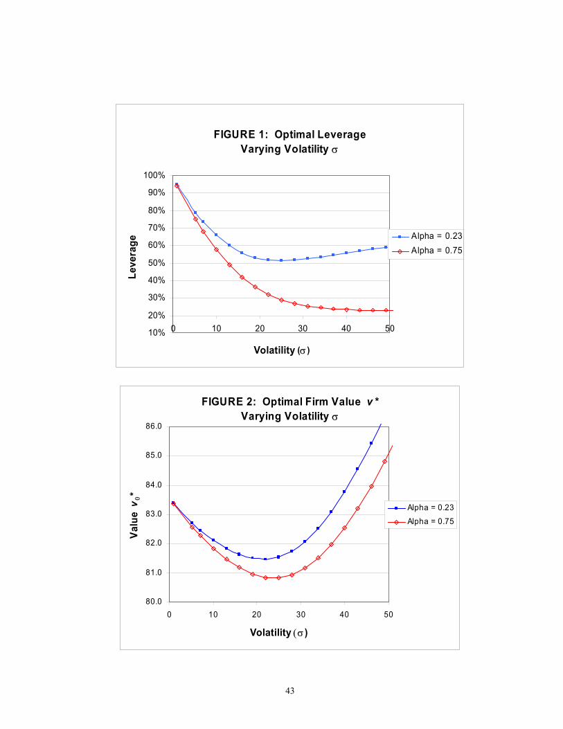
43

FIGURE 1: Optimal LeverageVarying Volatility σ

10%

20%

30%

40%

50%

60%

70%

80%

90%

100%

0 10 20 30 40 50

Volatility (σ )

Leve

rage

Alpha = 0.23Alpha = 0.75

FIGURE 2: Optimal Firm Value v *Varying Volatility σ

80.0

81.0

82.0

83.0

84.0

85.0

86.0

0 10 20 30 40 50

Volatility (σ )

Valu

e v 0

*

Alpha = 0.23

Alpha = 0.75

44

FIGURE 3A: Merger BenefitsVarying Correlation of Firms

-2.00%

-1.00%

0.00%

1.00%

2.00%

3.00%

4.00%

5.00%

0.00 0.20 0.40 0.60 0.80 1.00

Correlation

Perc

ent M

erge

r Be

nefit

s

Measure 1Measure 2Measure 3

FIGURE 3B: Merger BenefitsVarying Correlation of FirmsVolatility of Both Firms 24%

-1.50%

-1.00%

-0.50%

0.00%

0.50%

1.00%

1.50%

0.00 0.20 0.40 0.60 0.80 1.00

Correlation

Perc

ent M

erge

r Be

nefit

s

Measure 1Measure 2Measure 3

45

FIGURE 4: Merger Benefits Varying Joint Volatility σ

-20%

-15%

-10%

-5%

0%

5%

10%

0 10 20 30 40 50

Volatility (σ1 = σ2 = σ )

Perc

ent M

erge

r Be

nefit

s

Measure 1Measure 2Measure 3

FIGURE 5A: Merger Benefits Varying Size of Target as Percent of Firm 1

-1.00%

0.00%

1.00%

2.00%

3.00%

10% 25% 40% 55% 70% 85% 100%

Firm 2 Size as Percent of Firm 1

Per

cent

Mer

ger B

enef

its

Measure 1Measure 2Measure 3

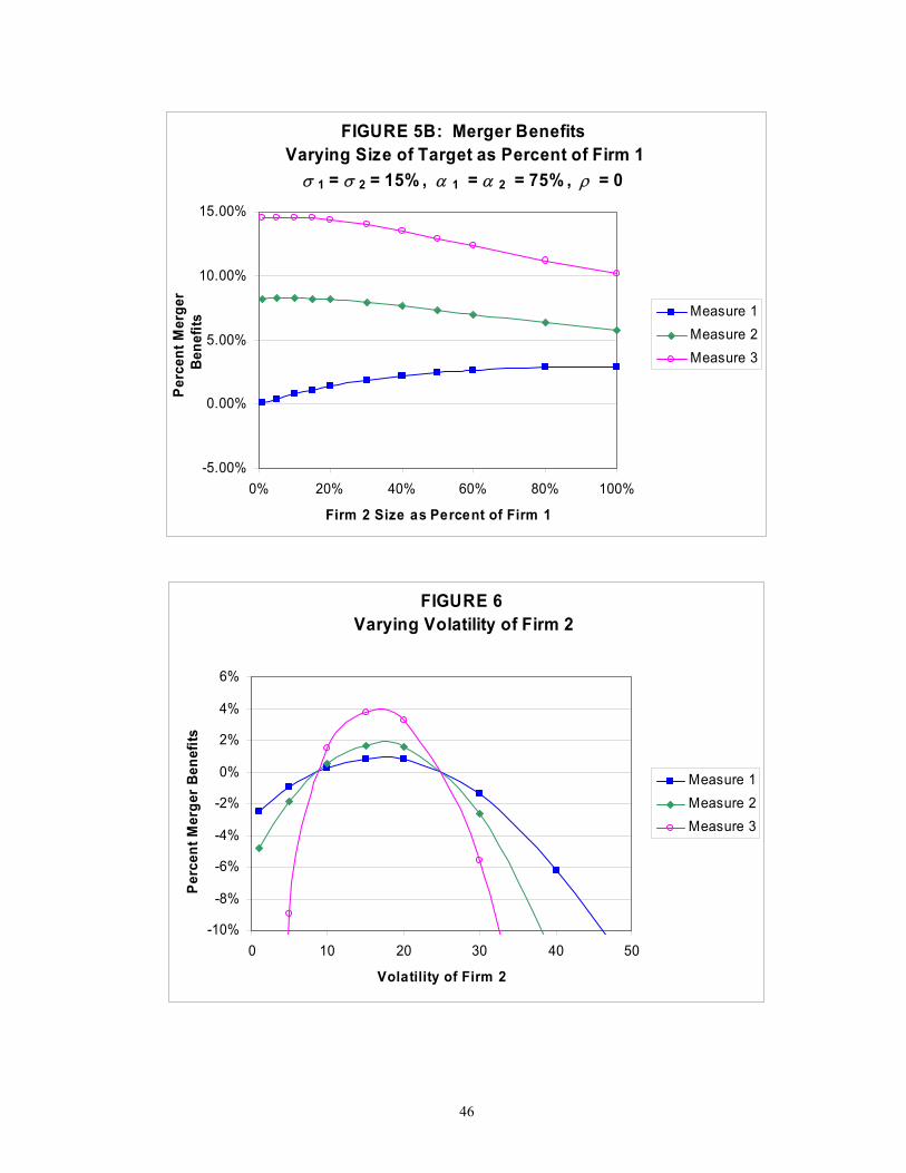
46

FIGURE 5B: Merger Benefits Varying Size of Target as Percent of Firm 1

σ 1 = σ 2 = 15% , α 1 = α 2 = 75% , ρ = 0

-5.00%

0.00%

5.00%

10.00%

15.00%

0% 20% 40% 60% 80% 100%

Firm 2 Size as Percent of Firm 1

Perc

ent M

erge

r B

enef

its

Measure 1Measure 2Measure 3

FIGURE 6 Varying Volatility of Firm 2

-10%

-8%

-6%

-4%

-2%

0%

2%

4%

6%

0 10 20 30 40 50

Volatility of Firm 2

Perc

ent M

erge

r Be

nefit

s

Measure 1Measure 2Measure 3

47

FIGURE 7 Varying Volatility of Firm 2

Decomposition of Measure 1 Synergies

-10%

-8%

-6%

-4%

-2%

0%

2%

0 10 20 30 40 50

Volatility of Firm 2

Abs

olut

e M

erge

r Ben

efits

Total (Measure 1)

Sarig Effect

Leverage Effect

FIGURE 8Optimal Value v * as a Function of Volatility σ

S

5.2 16

Z

X

Y

σS

v* (σS)

W

80.0

81.0

82.0

83.0

84.0

85.0

86.0

0 10 20 30 40 50

Volatility (σ )

Valu

e v *

48

FIGURE 9: Percent Merger BenefitsVarying Firm 2 Default Costs

Correlation ρ = 0.50

-2.50%

-2.00%

-1.50%

-1.00%

-0.50%

0.00%

0.50%

1.00%

0.00 0.20 0.40 0.60 0.80 1.00

Default of Firm 2 (α 2)

Perc

ent M

erge

r Be

nefit

s

Measure 1Measure 2Measure 3

Figures come from FinalPaperNew files