PULSES, FRONTS AND CHAOTIC WAVE TRAINS IN …chua/papers/Kazantsev97.pdf · PULSES, FRONTS AND...

Papers

International Journal of Bifurcation and Chaos, Vol. 7, No. 8 (1997) 1775–1790c© World Scientific Publishing Company

PULSES, FRONTS AND CHAOTIC WAVE TRAINSIN A ONE-DIMENSIONAL CHUA’S LATTICE

V. B. KAZANTSEV, V. I. NEKORKINThe Nizhny Novgorod State University

23 Gagarin Ave., 603600 Nizhny Novgorod, Russia

M. G. VELARDEInstituto Pluridisciplinar, Universidad Complutense,

Paseo Juan XXIII, No 1, Madrid 28 040, Spain

Received March 2, 1997; Revised September 20, 1997

We show how wave motions propagate in a nonequilibrium discrete medium modeled by a one-dimensional array of diffusively coupled Chua’s circuits. The problem of the existence of thestationary wave solutions is reduced to the analysis of bounded trajectories of a fourth-ordersystem of nonlinear ODEs. Then, we study the homoclinic and heteroclinic bifurcations ofthe ODEs system. The lattice can sustain the propagation of solitary pulses, wave fronts andcomplex wave trains with periodic or chaotic profile.

1. Introduction

Many systems modeling processes in nonequilib-rium excitable media are known to display solu-tions localized in space and steadily translating.Solitary pulses, fronts and wave trains propagatingwith a constant velocity are particular cases. Exam-ples come from all areas of science and engineering.Take, for instance, waves in fluids [Nepomnyashchy& Velarde, 1994], concentration waves in oscilla-tory reaction–diffusion systems [Zhabotinsky, 1974;Kuramoto, 1984], waves in optical fibers [Hasegawa& Kodama, 1995; Huang & Velarde, 1996], pulsesand pulse trains in long arrays of Josephson junc-tions [Lonngren & Scott, 1995], transmission ofexcitation in neural fibers [Murray, 1993], etc. Mod-els allowing to describe such processes are appro-priate Ginzburg–Landau equations [Van Saarloos& Hohenberg, 1992], the Korteweg de Vries equa-tion [Nekorkin & Velarde, 1994; Velarde et al., 1995;Christov & Velarde, 1995], the model of Fitz–HughNagumo [Murray, 1993] and their generalizations[Nepomnyashchy & Velarde, 1994].

There has also been growing interest in modelscomposed of coupled nonlinear oscillators located

at the junctions or sites of a space lattice. Suchsystems are also appropriate models for continuousmedia describing well, for example, the phenomenaof pattern formation [Nekorkin & Chua, 1993], wavepropagation [Perez–Munuzuri et al., 1993; Nekorkinet al., 1995, 1996] and spatially chaotic or spatio–temporal chaotic processes [Ogorzalek, 1995; Neko-rkin et al., 1995]. On the other hand, lattice modelsnaturally arise when using arrays of Josephson junc-tions, arrays of reaction cells, neural networks, ar-rays of electronic oscillators, etc., whose dynamicalbehavior can be quite complex both in time and inspace [Perez–Munuzuri et al., 1993; Winfree, 1991;Nekorkin et al., 1995; Perez Marino et al., 1995].Such lattices correspond to discrete nonequilibriummedia. Finally, such models can be used suitably forsimulation of a given natural process by means of,for example, appropriate electronic circuits whichwould exhibit a required collective behavior. Thisis of great importance both from the applied view-point and for the understanding of dynamical pro-cesses in nature.

We study the dynamics of a one-dimensionalarray of diffusively coupled Chua’s circuits [Chua,

1775

1776 V. B. Kazantsev et al.

1993; Madan, 1993]. In recent studies such arrayhas been used for modeling biological fibers, neu-ral networks, reaction–diffusion systems, etc. Ithas been found that the array can exhibit patternformation or spatial disorder, propagation of wavefronts, reentry initiation of pulses in two coupledarrays, spiral and scroll waves in two-dimensionalarrays, etc. The possibility of traveling pulses andwave trains has been shown in [Nekorkin et al.,1995] for the case of inductive coupling betweencells. However, generally these solutions althoughmay be long lasting structures they are not stable.In this paper we discuss this problem for the caseof resistive, diffusive coupling and show how thearray can be considered as an excitable “fiber” ca-pable of sustaining the propagation of various typesof stable travelling waves including single pulses orfronts and complex wave trains with a periodic or achaotic sequence of pulses. The profiles of possibletravelling waves are derived as bounded trajectoriesof the fourth-order system of ODEs underlying theoriginal space-dependent problem.

2. Model

The dynamics of 1-D lattice of diffusively cou-pled Chua’s circuits can be described in dimension-less form by the following set of ODEs (see e.g.[Nekorkin & Chua, 1993]):xj = α(yj − xj − f(xj)) + d(xj−1 − 2xj + xj+1)

yj = xj − yj + zj

zj = −βyj − γzj(1)

j = 1, 2, . . . , N ,

where f(x) describes the symmetric three-segmentpiecewise-linear function

f(x) =

bx− a− b if x ≥ 1

−ax if − 1 < x < 1

bx+ a+ b if x ≤ −1

(2)

with a > 0 and b > 0. The other parameters ofthe system α, β, γ, d are also taken positive. Weshall consider two types of boundary conditions:(i) zero-flux conditions x0 = x1, xN+1 = xN , and(ii) periodic conditions x0 = xN , xN+1 = x1. Thelatter describes a circular array.

The system (1) has three equilibria or fixedpoints corresponding to the homogeneous steady

states of the array. These states are

O : {xj = yj = zj = 0} ,P+ : {xj = x0, yj = y0, zj = z0} ,P− : {xj = −x0, yj = −y0, zj = −z0} .

where

x0 =(b+ a)(γ + β)

(γb+ β(b+ 1)),

y0 =(b+ a)γ

(γb+ β(b+ 1)),

z0 = − (b+ a)β

(γb+ β(b+ 1)).

It has been already shown in [Nekorkin et al., 1993]that for each set of the parameter values the “outer”states P− and P+ are locally asymptotically sta-ble while the trivial state O is unstable. Thusthe array is a discrete medium with two excitablesteady states. We now show that this medium isable to sustain stable localized solutions (fronts,pulses, pulse trains) travelling in space with definitevelocity.

3. Possible Profiles of Travelling Waves

Here we prove the existence of travelling wavesolutions in the system (1) and determine somecharacteristics of the waves (profile form, velocityof propagation).

3.1. Travelling waves

Let us look for a solution of the system (1) in theform of a travelling wave. We pose

xj(t) = x(ξ)

yj(t) = y(ξ)

zj(t) = z(ξ) ,

(3)

where ξ = t + jh is a coordinate moving alongthe array with a constant velocity c = 1/h. Thus,(x(ξ), y(ξ), z(ξ)) describes a space profile steadilytranslating with the velocity c. For solutions of theform (3) the system (1) is reduced to

x = α(y − x− f(x)) + d(x(ξ − h)

− 2x(ξ) + x(ξ + h))

y = x− y + z

z = −βy − γz

(4)

Pulses, Fronts and Chaotic Wave Trains in a One-Dimensional Chua’s Lattice 1777

where the dot denotes the differentiation with re-spect to the moving coordinate ξ. In the continuumapproximation (see e.g. [Nekorkin et al., 1995]),i.e. when the spatial grid of the solution profile issignificantly finer than the spatial grid of the dis-crete array, it is possible to change the differenceterm in Eq. (4) by using the second derivative x.Then, after simple transformations we obtain fortraveling waves the following fourth-order systemof ODEs:

x = u

ku = u− α(y − x− f(x))

y = x− y + z

z = −βy − γz

(5)

where k = d/c2 is a parameter characterizing thedependence of the velocity of the waves on the mag-nitude of the diffusion d.

Any bounded trajectory of the system (4) de-termines the possible profile of a traveling wavewhich steadily translates along the array with a con-stant velocity. The trivial translating solutions —homogeneous steady states O, P± of the array —correspond to the steady points of the system (4)which we denote by the same letters O, P±, respec-tively. Nontrivial solutions homoclinic to the pointsP± define solitary pulses propagating with respectto the “background” steady states P±, respectively.Orbits which asymptotically tend with ξ → ±∞ tothe different steady points (heteroclinic orbits) cor-respond to the traveling fronts selecting the termi-nal homogeneous stable state of the arrays. Thesystem (4) admits various homoclinic and hetero-clinic solutions and, besides, solutions of extremelycomplex profile, as we see further below.

3.2. Phase space analysis

Let us analyze the properties of the trajectories ofthe system (4) before embarking in the study ofhomoclinic and heteroclinic bifurcations.

Note, first, that by the symmetry properties ofthe function f(x), the vector field of the system (4),is invariant under space reflection

(x, u, y, z)→ (−x, −u, −y, −z) . (6)

Hence, for any given trajectory of the system(4) another trajectory defined by this transforma-tion coexists in the phase space. For instance,

if there appears a homoclinic orbit of the steadypoint P+, the orbit homoclinic to the point P−

also appears, and its profile is defined by the spacereflection (6).

Due to the piecewise-linearity of the functionf(x), the four-dimensional phase space of the sys-tem (4) can be divided in three regions. In each ofthese regions, motions are governed by linear sys-tems. The planes making this division are

U+ : {x = 1} and U− : {x = −1} .

In each linear region the dynamics of the system(4) is defined only by four eigenvalues of the linearmatrix and their corresponding eigenvectors whichdefine the manifolds of the steady points O, P±.

Let the parameters of the array unit be {a =1.5, b = 2, β = 0.5, γ = 0.01} and take {α, k} asthe control parameters. For each {α > 0, k > 0} itcan be shown that the eigenvalues corresponding tothe “outer” points P± are

{λ1 > 0, λ2 < 0, λ3, 4 = −h+ iω(h > 0)} .

Then, the points P± have a one-dimensional unsta-ble manifold Wu(P±) and a three-dimensional sta-ble manifold Ws(P

±).1 Within the correspondinglinear regions the Ws(P

±) represents the separa-trix plane in the four-dimensional phase space andWu(P±) the line containing point P± and two half-lines W1 and W2 extending to the different sidesof separatrix plane. Figure 1 illustrates qualita-tively the arrangement of the manifolds Ws(P

+)and Wu(P+) relative to the division plane U+ inthe phase space of the system (4). Let us denoteby M+

u the intersection point of the half-line W1

and the plane U+, and by l+s the line of intersectionof the separatrix plane Ws(P

+) and the plane U+.By the symmetry property (6) of the system (4) thepoint M−u and the line l−s with analogous propertiesare well defined in the plane U−

M±u : {Wu(P±) ∩ U±} ,

l±s : {Ws(P±) ∩ U±} .

The line l±s divides its neighborhood in the planeU± in two regions which we denote by D±∞ andD±n as shown in Figs. 1(a) and 1(b). The trajec-tories intersecting U± within D±∞ travel “above”

1The steady point O depends on control parameters. It can be either asymptotically stable (all eigenvalues have negative realpart) or saddle (saddle-focus) with two eigenvalues having positive real parts.


(a) (b)

Fig. 1. Manifolds of the steady point P± in the phase space of the system (4). (a) Qualitative behavior of the trajectoryforming a homoclinic loop and neighboring trajectories. If the point M+

u is mapped to a point of: (i) the region D+∞ —

the trajectory runs to infinity; (ii) the region D+n — the trajectory is going to make the next loop; (iii) the line l+s — the

homoclinic bifurcation occurs. (b) Qualitative behavior of the trajectory forming a heteroclinic linkage and its neighboringtrajectories.

the plane Ws(P±) and run to infinity, while those

going through the region D±n remain “below” theplane Ws(P

±) and after some time will return backto the plane U±.

3.3. Homoclinic and heteroclinic orbits

3.3.1. Homoclinic bifurcation

Consider, first, how the orbit homoclinic to thesteady point P+ is formed in the system (4). Itcorresponds to the time-dependent solution of thesystem (4) which asymptotically tends to the steadypoint as ξ → ±∞. Such solution is the trajectorythat simultaneously belongs to the unstable mani-fold Wu(P+) and to the stable manifold Ws(P

+) ofthe steady point P+. This trajectory should con-tain the point M+

u and intersect, at the same time,the line l+s . Therefore, the condition of exsistence ofhomoclinic orbits of the point P+ can be formulatedin the following way. Let the initial conditions of thesystem (4) be at the point M+

u . Then, if the flow

corresponding to (4) maps the point M+u to some

point M+s ∈ U+ and this point belongs to the line

l+s , then a homoclinic loop Γ appears in the phasespace of the system (4).

Let us change the control parameters in a smallneighborhood of the point of homoclinicity. Thenthe mapped point M+

s can shift from the line l+seither to the region D+

∞ or to the region D+n . In the

first case the trajectory started at M+u will tend to

infinity as shown in Fig. 1 (a) but in the secondcase this trajectory will go to a small neighborhoodof the point P+, then intersect the plane U+ nearthe point M+

u , hence the possibility of multi-loophomoclinic orbits near a given loop. According toShilnikov theorem [Shilnikov, 1969; Shilnikov, 1970]this possibility occurs if the saddle quantity σ of thesaddle-focus P+ defined as

σ = λ1 + max {λ2, h}

is positive for the parameters of homoclinicity.By the earlier mentioned symmetry with the

appearance of a loop homoclinic to the steady point


P+, there also appears a loop homoclinic to thesteady point P−, and the profile of the loop is de-fined by the transformation (6).

3.3.2. Heteroclinic bifurcation

Consider the possibility of heteroclinic orbitsformed by the steady points P+ and P−. Such or-bits correspond to a solution of the system (4) thatsimultaneously belongs to the unstable manifold ofthe point P+ [Wu(P+)] and to the stable manifoldof the point P− [Ws(P

−)]. This condition indicatesthe solution which contains the point M+

u and in-tersects the line l−s at some point M−s . Thus, theparameters for which the flow (4) maps the pointM+u to some point M−s ∈ U− which belongs to the

line l−s correspond to the appearance of a hetero-clinic orbit H± “linking” the steady points P+ andP−.

Applying the transformation (6) to the or-bit H± we obtain the heteroclinic orbit H∓ that“started” at the point P− and tends to the pointP+. Thus, there exists a contour P+ → H± →P− → H∓ → P+ in the phase space of the sys-tem (4) [see Fig. 1(b)] [Turaev, 1996; Shashkov &Turaev, 1996]. We show below that this contour isassociated with the existence in the medium of soli-tary pulses originated from two fronts (kinks) eachof which is described by the heteroclinic orbits H±and H∓ taken separately.

3.4. Bifurcation set

To define the parameters corresponding to thehomoclinic and heteroclinic bifurcation for fixedk = k∗, we calculate the split function which is

SΓ(α) = dev(M+s , l

+s )

for a homoclinic loop Γ, and

SH±(α) = dev(M−s , l−s )

for a heteroclinic orbit H±. The sign dev denotesthe deviation of a point from a line. The param-eter α∗ corresponding to a zero of the split func-tion determines the bifurcation point (α∗, k∗) inthe state space (α, k). The location of the linesl±s and the points M±u is obtained analytically as it

has been done in [Nekorkin et al., 1995]. The mapM+u →M±s is determined by numerical integration

of the system (4).Let us turn to Fig. 2 where the bifurcation dia-

gram is displayed. We denote the bifurcation curvesby the letters Γ and H. A superscript n indicatesthe number of loops made by the orbit and thesubscript s or l characterizes the “magnitude” ofthe pulse (“s” — small, “l” — large). Figure 2(a)shows the diagram in rather large scale in (α, k)plane. Two close curves Γ1

l and H1l correspond to

the simplest types of homoclinic and heteroclinicorbits. The shapes of the orbits in the phase spaceand their profiles (x(ξ)) are displayed in Fig. 3 andare marked by the same letters as the correspondingbifurcation curves (see Fig. 3(a) for profiles of thesimplest orbits Γ1

l , H1l and Γ1

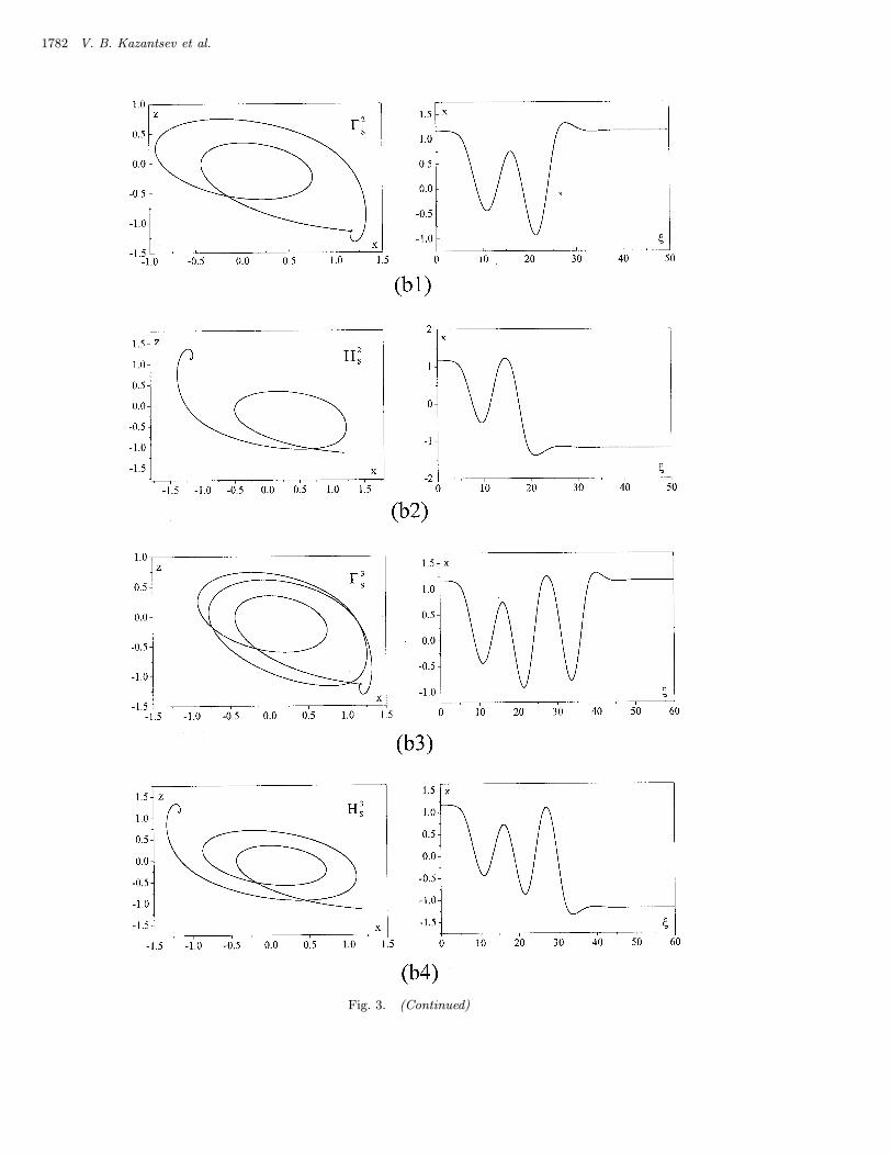
s). For large enoughvalues of k there exists a number of homo- and het-eroclinic bifurcations corresponding to the pulses of“small magnitude” (the curves marked by lettersHns and Γns in Fig. 2).2 As earlier said “n” indi-

cates the number of turns made by the orbits nearthe steady point O. Some profiles of multi-rotatedorbits are given in Fig. 3(b).

The dashed curve in Fig. 2 corresponds to thebifurcation of the equilibrium O, hence this pointbecomes a stable focus (to the right of the dashedcurve) with two pairs of complex eigenvalues. Inthis region the trajectory Wu(P+) (see Fig. 1) isattracted by the stable point O hence multi-rotatedhomoclinic orbits do not appear for such parame-ters. In this case the solution formed by Wu(P+)is also bounded (“connects” the points P+ and O)hence corresponds to a possible travelling wave inthe array (1). However, as earlier noted the homo-geneous equilibrium state of the array correspond-ing to the point O is unstable. Then such wavesolutions are also unstable.

Having calculated the saddle quantity σ ofthe saddle-focus P+ we find that it has a posi-tive value for each point of all bifurcation curvesassociated with single-loop homoclinic bifurcation(Γ1l , Γ1

s, Γ2s, Γ3

s, . . .). Hence, according to theShilnikov theorem for the parameters varying in asmall neighborhood of each curve there occurs anumber of homoclinic bifurcations resulting in theappearance of multi-loop homoclinic orbits. Be-sides, the neighborhood of the homoclinicity in thephase space contains a countable set of hyperbolic

2We distinguish the large and small orbits in the following way. Each loop of the large orbit of P+ extends to the “opposite”outer linear region intersecting both planes U− and U+, while the small loops have intersections with the plane U+ only.


Fig. 2. Bifurcation diagram for homoclinic Γnl, s and heteroclinic Hns, l orbits in the (k, α) parameter plane. The superscript

n indicates the number of rotations or loops made by an orbit in the phase space (or the number of humps along the profileof the orbit). The subscript s or l distinguishes the orbits with all loops of large “magnitude” and those containing at leastone loop of small “magnitude”. (a) Full diagram. (b) and (c) Two enlarged regions.


Fig. 3. Orbits in phase space and their corresponding profiles for different points of the bifurcation diagram. (a) Thesimplest, single-loop homoclinic and heteroclinic orbits. (a1) The orbit Γ1

l for α = 1.500, k = 1.624; (a2) The orbit H1l ,

α = 1.502, k = 1.622; (a3) The orbit Γ1s; α = 1.501, k = 4.324; (a4) The orbit Γ1

l , α = 0.610, k = 5.300. Dashed curvesshow the symmetric orbits that also exist in the system (4). (b) Multi-rotated orbits of small “magnitude” and correspondingwave profiles. (b1) Γ2

s, α = 1.503, k = 5.576; (b2) H2s , α = 1.502, k = 4.405; (b3) Γ3

s, α = 1.502, k = 5.706; (b4) H3s ,

α = 1.500, k = 5.824. (c) The profiles of multi-looped orbits of large “magnitude”. (c1) Γ2l , α = 0.620, k = 5.304; (c2) Γ3

l ,α = 0.618, k = 5.301; (c3) Γ4

l , α = 0.618, k = 5.302; (c4) Γ5l , α = 5.301, k = 0.618; (c5) H2

l , α = 0.615, k = 5.300; (c6) H3l ,

α = 0.617, k = 5.301.


Fig. 3. (Continued)


Fig. 3. (Continued)

periodic orbits. Figures 2(b) and 2(c) present twoenlarged regions taken near the bifurcation curveΓ1l . Here different multi-loop orbits can be distin-

guished. The profiles of the multi-loop orbits aredepicted in Fig. 3(c).

As it has been earlier mentioned the hetero-clinic bifurcation H1

l yields the appearance of theheteroclinic contour in the phase space of the sys-tem (4). We find that the neighborhood of the curveH1l contains a number of bifurcation points which

correspond to the appearance of single- and multi-loop homoclinic orbits Γn. The profile of each loopof these orbits is “constructed” from two symmetricheteroclinic orbits taken from the contour [see the

simplest one Γ1 in Fig. 3(a)]. Besides, there existsolutions having the form of multi-loop heteroclinicorbits. Figure 3(c) illustrates the examples of suchorbits for n = 2, 3 loops.

In summary: The fourth order system (4)describing the profiles of possible travelling waves


in the array (1) allows a wide variety of boundedsolutions. These are

• Single- and multi-loop homoclinic orbits withdifferent “magnitude”;• Multi-rotated homoclinic orbits;• Heteroclinic orbits of different form;• Homoclinic solutions arising from two symmetric

heteroclinic orbits;• Periodic orbits of hyperbolic type with quite com-

plex profile (that occur near each homoclinicity).

Each of these solutions ensures the existence of awave with a definite profile which propagates alongthe array with constant velocity c = 1/h. However,the investigation of the system (4) does not ensuretheir stability.

4. Excitation and Evolution ofSolitary Pulses and Fronts

Let us assume that the discrete medium modeledby (1) initially has been in a stable equilibriumassociated with the homogeneous state P+. Howshould we perturb this state to observe, for ex-ample, a travelling pulse associated with an orbitof the system (4) homoclinic to the steady pointP+? As earlier shown, near a given loop there ex-ist multi-loop orbits whose profiles determine themulti-hump pulses. Thus, for a given set of param-eter values there can propagate a number of differ-ent travelling waves. To differentiate these waveswe construct the initial excitation of the state P+

as close as possible to the profile of a given homo-clinic orbit. If the pulse is stable we will observe inthe simulation the steady translation of the initialprofile along the array. If this pulse is unstable itwill go to another attractor of the system (1).

4.1. Construction of the wave profiles

Let us take a point (α∗, k∗) of the bifurcation curvecorresponding, for instance, to a homoclinic orbitΓ1l . The space profile of the solitary pulse associ-

ated with this orbit can be constructed by using (3)with ξ = jh from the profile of the homoclinic orbit(x(ξ), y(ξ), z(ξ)). Let us take the core of this pro-file of “length” T (ξ ∈ [ξ0, ξ0 +T ]) that satisfies thecondition

|x(ξ)− x0| � 1 , |y(ξ)− y0| � 1 ,

|z(ξ) − z0| � 1

∀ξ < ξ0 , ξ > T + ξ0 .

Hence the “tails” of the pulse are close enough tothe steady state P+.

Then, we perturb the homogeneous stable stateP+ by “forcing” N1 elements (N1 = T/h) in the ar-ray starting from the element k0 and mimicking theprofile of the homoclinic orbit

xk+k0(t = 0) = x(ξ0 + kh) ,

yk+k0(t = 0) = y(ξ0 + kh) ,

zk+k0(t = 0) = z(ξ0 + kh)

with k = 1, . . . , N1. We use such space distributionas the initial condition for the numerical simulationof the system (1) to study the evolution of travellingwaves.

Note, that to satisfy the continuum approxima-tion which we used to obtain the system (4), the pa-rameter h should be chosen small enough (h � T )to ensure the necessary smoothness of the wave pro-file. Then, the value of the diffusion coefficient d,d = k∗

h2 , appears rather large.

4.2. Stable and unstable solitary pulses

Figures 4 illustrate the evolution of the solitarypulses associated with the homoclinic orbits of large“magnitute” (obtained from the curves Γnl of the bi-furcation diagram). Figure 4(a) shows a single pulse(orbit Γ1

l ), Fig. 4(b) — a two-humps pulse (orbit Γ2l )

and Fig. 4(c) — a five-humps pulse (orbit Γ5l ). With

the initial distributions close to the homoclinic orbitprofile in the way described above we observe thesolutions which travel along the array with constantvelocity and no apparent change of form. For zero-flux boundary conditions the pulses are absorbedby the boundary and the terminal state (as t→∞)of the array becomes the homogeneous state P+.The circular array exhibits stable pulses propagat-ing around the circle. These pulses represent wavesof cnoidal type whose images in the phase space ofthe system (4) are hyperbolic periodic orbits which,according to Shilnikov theorem occur near homo-clinicity with positive saddle quantity.

Note, that due to symmetry there can propa-gate solitary pulses of inverse profiles relative to the“background” homogeneous state P−. In the termi-nology used in the field of optical fibers [Hasegawa& Kodama, 1995; Huang & Velarde, 1996] we cansay that the discrete medium (1) allows the propa-gation of both “bright” and “dark” pulses of widevariety of spatial forms.


Fig. 4. Space-time evolution of stable, large “magnitude” pulses. For the numerical simulation of the discrete medium,the array has been initially forced by a disturbance close to the profile of the homoclinic orbits of the system (4).(a) Single-hump pulse, α = 0.627, d = 133. (b) Two-hump pulse, α = 0.620, d = 133. (c) Five-hump pulse, α = 5.301, d = 59.

Consider, now, the behavior of solitary pulsesassociated with homoclinic orbits of a small “mag-nitude” (curves Γns in Fig. 2). All pulses of suchtype appear unstable in the numerical simulationof the array (1). Figure 5 illustrates, the two waysof evolution of the single pulse of the small am-plitude Γ1

s for two parameter sets. The first caseprovides the decay of the small pulse to the “back-ground” homogeneus state P+ [Fig. 5(a)], but inthe second one the pulse evolves to the stable waveof large “magnitude” [Fig. 5(b)] which is associatedwith the homoclinic orbit Γ1

l . It means that de-pending on parameter values the initial excitationcan fall either into the basin of attraction of the ho-mogeneous, stable steady state P+, or in the stablesolitary pulse.

Note, that the solitary pulses of large “mag-nitude” could be excited from many initial distur-bances. Figure 5(c) illustrates the appearance of

two solitary pulses from rather simple initial condi-tions (a part of the elements has been initially atthe state P+, and the other part at the state P−).

4.3. Wave fronts and pulses constructedfrom two fronts

Together with the single and multi-hump pulses, thearray (1) can exhibit other travelling wave fronts(kinks) associated with the heteroclinic orbits of thesystem (4). These solutions can be interpreted asthe transient process in the “selection” of a terminalstable homogeneous state, P+ or P−. The evolu-tion of the single and two-hump fronts is illustratedin Figs. 6(a), 6(b). The profiles of these frontsare derived from the heteroclinic orbits H1

l , H2l .

The fronts whose profiles contain humps of small“magnitude” (curves Hn

s of Fig. 2) become unsta-ble and evolve to the simplest front (H1

l ), i.e. they


Fig. 5. Evolution of the initial condition derived from the homoclinic orbits of small “magnitude”. (a) Decay of the pulseto the “background” steady state. Parameter values: α = 0.66, d = 6.5. (b) Transformation of a small “magnitude” pulse toa stable pulse large “magnitude”. Parameter values: α = 2.00, d = 52. (c) Onset of two stable pulses traveling in oppositedirections from initial conditions taken in the form of pedestal. Parameter values: α = 3.74, d = 10.

are unstable like the solitary pulses of small “mag-nitude” [see, e.g. Fig. 6(c)].

As predicted in the previous section, pulseswhose profiles are composed of two symmetricfronts can be propagated. The initial condi-tions for such waves can be derived from a ho-moclinic orbit Γ1

l or in a simple way by takingthe two symmetric kinks with a finite delay. Suchfronts are stable if the constituent fronts are sta-ble. Figure 6(d) illustrates the evolution of apulse composed of two stable two-hump fronts.

In summary, the discrete medium modeledby the system (1) allows stable wave solutionsof extremely diverse profiles including “dark” and“bright” pulses of single and multi-hump forms,kinks and “anti”-kinks (associated with symmetricheteroclinic orbits), multi-hump fronts and pulsescomposed of several set of fronts. Note, that allthis diversity of wave motions could be realizedfor the same parameter values of the array (1),and all waves would propagate with almost equalvelocities.3

3For a given d > d0 there exists hi < h0 to hit any bifurcation point (α∗, k∗i ) corresponding to ith type of travelling waves.For the large “magnitude” waves all ki will be localized between the curves H1

l and Γ1l for the fixed α = α∗ (see bifurcation

diagram Fig. 2).


Fig. 6. Space-time evolution of wave fronts whose profiles have been derived from the heteroclinic orbits of the system (4).The fronts provide the “selection” of the terminal (t → ∞) homogeneous steady state of the array P+ or P−. (a) Simplewave front associated with the orbit H1

l . Parameter values: α = 2.00, d = 15.2. (b) Stable multi-hump wave front (orbitH2l ). Parameter values: α = 0.615, d = 59. (c) Transformation of the unstable wave front associated with the orbit H2

s tothe simplest front (orbit H1

l ). Parameter values: α = 0.755, d = 56. (d) Stable localized structure consisting of two stablemulti-hump fronts. It can be interpreted as the multi-hump pulse associated with a homoclinic orbit from the family Γnl .Parameter values: α = 0.615, d = 33.

5. Construction of Chaotic Wave Trains

Let us now show how the discrete medium (1) al-lows the propagation of wave trains of extremelycomplex profile even with disordered or chaotic con-figuration.

Let us note, first, that the “tails” of all sta-ble pulses and fronts decay rather quickly along thespatial coordinates. As it has been earlier men-tioned the velocities of all large “magnitude” waves

are close to each other. Then, if in the array we puttwo different pulses (for example, a single pulse anda two-hump pulse) with a finite, rather long delay,they can form a bound state as a result of a weakinteraction between the initial pulses. This staterepresents the three-hump pulses traveling withconstant velocity (not equal, but close to the ve-locity of the initial pulses) (see e.g. [Christov &Velarde, 1995]). In the phase space of the system(4) this state appears as a three-loop homoclinic


orbit (or “three-loop” periodic orbit for the circulararray). Its existence near the loops with a positivesaddle quantity is ensured by the Shilnikov theo-rem. Complex wave trains composed of one- andtwo-hump pulses are shown in Fig. 7(a). Numericalintegration of the array (1) shows the stability ofthis train as expected. Indeed the wave “consistsof” two stable pulses.

Similarly, more complex wave trains can beconstructed. Consider a rather long array composedof numerous elements. Building the wave trainfrom a large number of stable pulses and fronts,which can propagate separately, we obtain a waveof rather complex profile. Note, that the delayor the distance in space between each neighbor-ing components could vary in very wide limits.

Fig. 7. Wave trains composed of a sequence of stable pulses and fronts for the parameters taken near α = 0.8, d = 11.75.(a) Interaction of single- and two-hump pulses ends up in a stable bound state. (b) Complex wave train composed of adisordered sequence of stable pulses and fronts. Its evolution corresponds to the numerical simulation in the circular array.


Extending the boundaries of the array to infinitywe can speak about the excitation of chaotic wavetrains in the system. These are profiles composedof a disordered sequence of pulses and fronts. Sucha sequence can be associated with the homoclinic(heteroclinic) orbit of an infinite number of loops ofthe system (4).

To investigate the evolution of chaotic trains weuse a circular array with a large enough number ofelements. In this case the disordered train appearsin the phase space (4) as a complex periodic orbitfrom the countable set (see Sec. 4). Putting in thearray, the initial condition in the form of an arbi-trary sequence of pulses and fronts, we find thatit tends to the stable solution steadily translatingalong the array [see Fig. 7(b)], i.e. hence a station-ary wave of complex profile.

In summary, the discrete medium modeled by(1) can sustain chaotic wave trains.

6. Conclusion

We have shown that a one-dimensional lattice ofChua’s circuits allows a wide variety of stable trav-eling wave solutions, from a simple solitary pulseor a wave front to quite complex long wave trains,“bright” and “dark” (optical) pulses or chaotic se-quences of pulses and fronts. The lattice repre-sents, in fact, a discrete medium whose propertiesare quite similar to a continuum, reaction–diffusionsystem with one diffusing component.

We have studied the possible traveling wavesand their stability by analyzing the underlyingfourth-order system of ODEs whose bounded solu-tions correspond to the profiles of the waves. Illus-tration of the actual wave profiles and wave trainsfound has been done by numerically simulating thedynamical system.

In conclusion, our results show the possibilityof using a lattice of Chua’s circuits as a tool for thedevelopment of information transmission channelsor for modeling wave processes in different areas ofscience and technology.

Acknowledgments

Part of this research was carried out while V. I.Nekorkin held a Sabbatical position with the In-stituto Pluridisciplinar at the Universidad Com-plutense. This research was supported by NATOunder Grant OUTR. LG 96–578, by DGICYT

(Spain) under Grant PB 93-81 and by INTAS underGrant 94–929.

ReferencesChristov, C. I. & Velarde, M. G. [1995] “Dissipative

solitons,” Physica D86, 323–347.

Chua, L. O. [1993] “Global unfolding of Chua’s circuits,”IEICE Trans. Fundamental Electron. Commun. Com-put. Sci. E76A5, 704–737.

Huang, G. & Velarde, M. G. [1996] “Head-on collisions ofdark solitons near the zero–dispersion point in opticalfibers,” Phys. Rev. E54, 3048–3051.

Hasegawa, A. & Kodama, Y. [1995] Solitons in OpticalCommunications (Oxford University Press, Oxford).

Kuramoto, Y. [1984] Chemical Oscillators, Waves andTurbulence (Springer–Verlag, Berlin).

Madan, R. N. (Ed.) [1993] Chua’s Circuit: A Paradigmfor Chaos (World Scientific, Singapore).

Murray, J. D. [1993] Mathematical Biology (Springer–Verlag, Berlin).

Nekorkin, V. I. & Chua, L. O. [1993] “Spatial disorderand wave fronts in a chain of coupled Chua’s circuits,”Int. J. Bifurcation and Chaos 3, 1282–1292.

Nekorkin, V. I. & Velarde, M. G. [1994] “Solitarywave, soliton bound states and chaos in a dissipativeKorteweg–de Vries equation,” Int. J. Bifurcation andChaos 4, 1135–1146.

Nekorkin, V. I., Kazantsev, V. B., Rulkov, N. F., Velarde,M. G. & Chua, L. O. [1995] “Homoclinic orbits andsolitary waves in a one-dimensional array of Chua’scircuits,” IEEE Trans. Circuits Syst. 42, 785–801.

Nekorkin, V. I., Kazantsev, V. B. & Velarde, M. G. [1996]“Travelling waves in a circular array of Chua’s cir-cuits,” Int. J. Bifurcation and Chaos 6, 473–484.

Nepomnyashchy, A. A. & Velarde, M. G. [1994] “A three-dimensional description of solitary waves and their in-teraction in Marangoni–Benard layers,” Phys. Fluids6, 187–198.

Ogorzalek, M. J., Galias, Z., Dabrowski, A. M. &Dabrowski, W. R. [1995] “Chaotic waves and spatio-temporal patterns in large arrays of doubly-coupledChua’s circuits,” IEEE Trans. Circuits Syst. 42,706–715.

Perez Marino, I., de Castro, M., Perez–Munuzuri, V.,Gomez–Gesteira, M., Chua, L. O. & Perez–Villar, V.[1995] “Study of Reentry Initiation in Coupled Paral-lel Fibers,” IEEE Trans. Circuits Syst. 42, 665–672.

Perez–Munuzuri, A., Perez–Munuzuri, V., Perez–Villar,V. & Chua, L. O. [1993] “Spiral waves on a 2-D arrayof nonlinear circuits,” IEEE Trans. Circuits Syst. 40,872–877.

Perez–Munuzuri, V., Perez–Villar, V. & Chua, L. O.[1993] “Travelling wave front and its failure in one-dimensional array of Chua’s circuits,” J. Circuits Syst.Comput. 3, 215–229.


Saarloos, W. & Hohenberg, P. C. [1992] “Fronts, pulses,sources and sinks in generalized complex Ginzburg–Landau equation,” Physica D56, 303–367.

Shashkov, M. V. & Turaev, D. V. [1996] “On the complexbifurcation set for a system with simple dynamics,”Int. J. Bifurcation and Chaos 6, 949–968.

Shilnikov, L. P. [1969] “On a new type of bifurcationof multidimensional dynamical systems,” Sov. Math.Dokl. 10, 1368–1371.

Shilnikov, L. P. [1970] “A contribution to the problem ofthe structure of an extended neighborhood of a roughequilibrium state of saddle-focus type,” Math. USSRSb. 10, 91–100.

Turaev, D. V. [1996] “On dimension of non-local bifur-cational problems,” Int. J. Bifurcation and Chaos 6,919–948.

Velarde, M. G., Nekorkin, V. I. & Maksimov, A. G. [1995]“Further results on the evolution of solitary waves andtheir bound states of a dissipative Korteweg-de Vriesequation,” Int. J. Bifurcation and Chaos 5, 831–839.

Winfree, A. T. [1991] “Varieties of spiral wave behav-ior: An experimantalist’s approach to the theory ofexcitable media,” Chaos 1, 303–334.

Zhabotinsky, A. M. [1974] Concentration Auto-oscillations (Nauka, Moscow) (Russian).

PULSES, FRONTS AND CHAOTIC WAVE TRAINS IN …chua/papers/Kazantsev97.pdf · PULSES, FRONTS AND...

Documents

Transcript of PULSES, FRONTS AND CHAOTIC WAVE TRAINS IN …chua/papers/Kazantsev97.pdf · PULSES, FRONTS AND...