HAL Id: hal-02369031https://hal.archives-ouvertes.fr/hal-02369031

Submitted on 18 Nov 2019

HAL is a multi-disciplinary open accessarchive for the deposit and dissemination of sci-entific research documents, whether they are pub-lished or not. The documents may come fromteaching and research institutions in France orabroad, or from public or private research centers.

L’archive ouverte pluridisciplinaire HAL, estdestinée au dépôt et à la diffusion de documentsscientifiques de niveau recherche, publiés ou non,émanant des établissements d’enseignement et derecherche français ou étrangers, des laboratoirespublics ou privés.

Pulsed flying spot with the logarithmic parabolasmethod for the estimation of in-plane thermal diffusivity

fields on heterogeneous and anisotropic materialsL Gaverina, J. Batsale, A Sommier, Christophe Pradere

To cite this version:L Gaverina, J. Batsale, A Sommier, Christophe Pradere. Pulsed flying spot with the logarithmicparabolas method for the estimation of in-plane thermal diffusivity fields on heterogeneous andanisotropic materials. Journal of Applied Physics, American Institute of Physics, 2017, 121 (11),pp.115105. �10.1063/1.4978919�. �hal-02369031�

Pulsed flying spot with the logarithmic parabolas method for the estimation of in-planethermal diffusivity fields on heterogeneous and anisotropic materialsL. Gaverina, J. C. Batsale, A. Sommier, and C. Pradere

Citation: Journal of Applied Physics 121, 115105 (2017); doi: 10.1063/1.4978919View online: http://dx.doi.org/10.1063/1.4978919View Table of Contents: http://aip.scitation.org/toc/jap/121/11Published by the American Institute of Physics

Pulsed flying spot with the logarithmic parabolas method for the estimationof in-plane thermal diffusivity fields on heterogeneous and anisotropicmaterials

L. Gaverina, J. C. Batsale, A. Sommier, and C. Praderea)

I2M-TREFLE, UMR CNRS 5295, Esplanade des arts et M�etiers 33405 Talence Cedex, France

(Received 27 January 2017; accepted 7 March 2017; published online 21 March 2017)

A novel thermal non-destructive technique based on a Pulsed Flying Spot is presented here by

considering in-plane logarithmic processing of the relaxing temperature field around the heat

source spot. Recent progress made in optical control, lasers, and infrared cameras permits the

acquisition of 2D temperature fields and localized thermal excitation on a small area instead of the

entire recorded image. This study focuses on a new method based on spatial logarithm analysis of a

temperature field to analyse and measure different parameters, such as the in-plane thermal

diffusivity and localization of the spot. In this paper, this method is presented and the first

results of heterogeneous anisotropic materials are depicted. The in-plane thermal diffusivity is

estimated with an error lower than 4%, and the initial location of the heating spot is determined.

Published by AIP Publishing. [http://dx.doi.org/10.1063/1.4978919]

I. INTRODUCTION

The use of new scanning systems based on a galvanome-

ter mirror allows the easy control of the spatial and temporal

displacements of a laser hot spot over a plane surface. Such

systems are then suitable for use in developing new flying

spot methods as alternatives to the initial flying spot tech-

nique,1–4 which is based on a constant velocity of the spot.

By contrast, instead of the single temperature measurement

used in Ref. 5, infrared (IR) thermography allows the tran-

sient temperature field measurement and direct processing of

a small area around the heating spot. Even if a great number

of pulsed spots are deposited, the preliminary step will con-

sist of analysing the effect of a unique spot. To implement

such processing, an analysis of the transient field of the

temperature response from the analytical expression has been

proposed. This method is very close and complementary to

the Thermographic Signal Reconstruction (TSR) method

used in the case of the 1D flash experiment.6 In fact, this tech-

nique used the time logarithm of the temperature field,

whereas the method proposed here is based on the spatial log-

arithmic processing of the temperature response. Other meth-

ods exist for in-plane thermal diffusivity estimation by using

the Fourier transform of the temperature field7–9 or by consid-

ering the transient evolution of the Gaussian temperature dis-

tribution.10,11 One drawback of these methods is the number

of pixels needed to perform inverse processing. The main

goal of this work is based on laser local heating (the heat spot

size is lower than the pixel size), and the idea is to propose a

method in which only a few pixels around the heating spot

are necessary to retrieve the thermal properties.

In this paper, some theoretical aspects are considered. A

new estimation method is then presented, and finally, experi-

mental data and results are shown to validate the capability

of the method by estimating the in-plane diffusivities, posi-

tion of the spot, and nature of the in-plane heat transfer in a

heterogeneous and anisotropic sample.

II. MATERIAL AND EXPERIMENTAL METHODS

A. Setup

The experimental setup in Figure 1 is composed of a

laser diode (wavelength 976 nm) of 330 mW power. To colli-

mate the laser beam, an optical collimator system (Thorlabs)

is used. A Dual-Axis Scanning Galvo System (Thorlabs

GVS112/M) was used to control the spatial displacement of

the laser spot. The principle of the laser beam deviation

towards the sample is shown in Figure 1. To focus the laser

beam on the surface, an f-theta scan lens was used with a

focusing length of 160 mm. With this focal length, the scan-

ning area is equal to a square of 11 cm� 11 cm, and the

resulting diameter of the focused spot is 26 lm with a mini-

mum displacement of 4.5 lm. In practice, the angular posi-

tions of the galvanometric system are related to a couple of

coordinates expressed as voltage (V). Indeed, the range of

angular positions included within �20� and 20� is discretized

in terms of voltage applied to the motor in the corresponding

range of �10 V to 10 V. Thus, the angular position calibra-

tion, applied voltage, and resulting displacement are set

according to the following relationship: DDf ¼ 2f tan Dhð Þ¼ 2f tan DV

2

� �.

This laser diode is mounted horizontally, and the beam

is reflected with a dichroic mirror (MD, treated to reflect

95% of the visible light from 700 nm to 1000 nm and to

transmit 95% of the infrared radiation between 2 and 16 lm).

To measure the temperature fields, an IR camera MCT

(FLIR SC7000, 320� 256 pixels, pitch 30 lm, and spectral

band from 7 to 14 lm) was used with an infrared objective

lens (focal 25 mm). Finally, the resulting spatial resolution is

approximately 250 lm per pixel.

a)Author to whom correspondence should be addressed. Electronic mail:

c.pradere@i2m.u-bordeaux1.fr

0021-8979/2017/121(11)/115105/8/$30.00 Published by AIP Publishing.121, 115105-1

JOURNAL OF APPLIED PHYSICS 121, 115105 (2017)

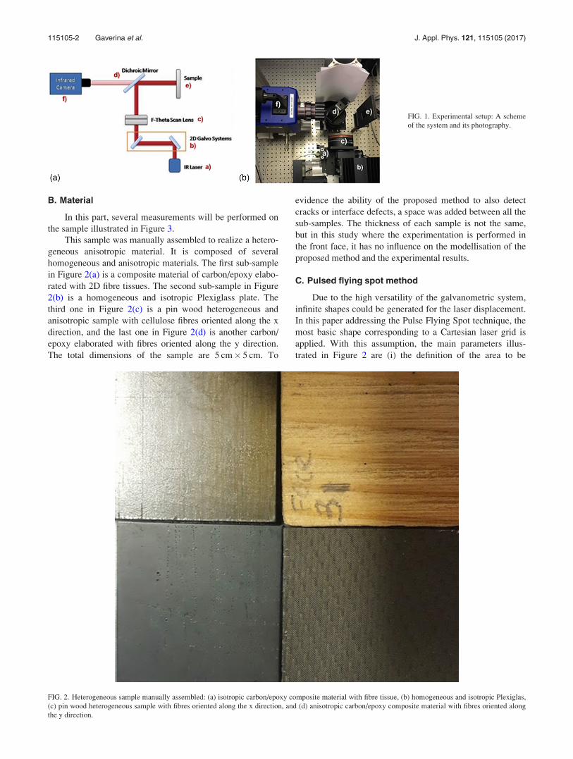
B. Material

In this part, several measurements will be performed on

the sample illustrated in Figure 3.

This sample was manually assembled to realize a hetero-

geneous anisotropic material. It is composed of several

homogeneous and anisotropic materials. The first sub-sample

in Figure 2(a) is a composite material of carbon/epoxy elabo-

rated with 2D fibre tissues. The second sub-sample in Figure

2(b) is a homogeneous and isotropic Plexiglass plate. The

third one in Figure 2(c) is a pin wood heterogeneous and

anisotropic sample with cellulose fibres oriented along the x

direction, and the last one in Figure 2(d) is another carbon/

epoxy elaborated with fibres oriented along the y direction.

The total dimensions of the sample are 5 cm� 5 cm. To

evidence the ability of the proposed method to also detect

cracks or interface defects, a space was added between all the

sub-samples. The thickness of each sample is not the same,

but in this study where the experimentation is performed in

the front face, it has no influence on the modellisation of the

proposed method and the experimental results.

C. Pulsed flying spot method

Due to the high versatility of the galvanometric system,

infinite shapes could be generated for the laser displacement.

In this paper addressing the Pulse Flying Spot technique, the

most basic shape corresponding to a Cartesian laser grid is

applied. With this assumption, the main parameters illus-

trated in Figure 2 are (i) the definition of the area to be

FIG. 1. Experimental setup: A scheme

of the system and its photography.

FIG. 2. Heterogeneous sample manually assembled: (a) isotropic carbon/epoxy composite material with fibre tissue, (b) homogeneous and isotropic Plexiglas,

(c) pin wood heterogeneous sample with fibres oriented along the x direction, and (d) anisotropic carbon/epoxy composite material with fibres oriented along

the y direction.

115105-2 Gaverina et al. J. Appl. Phys. 121, 115105 (2017)

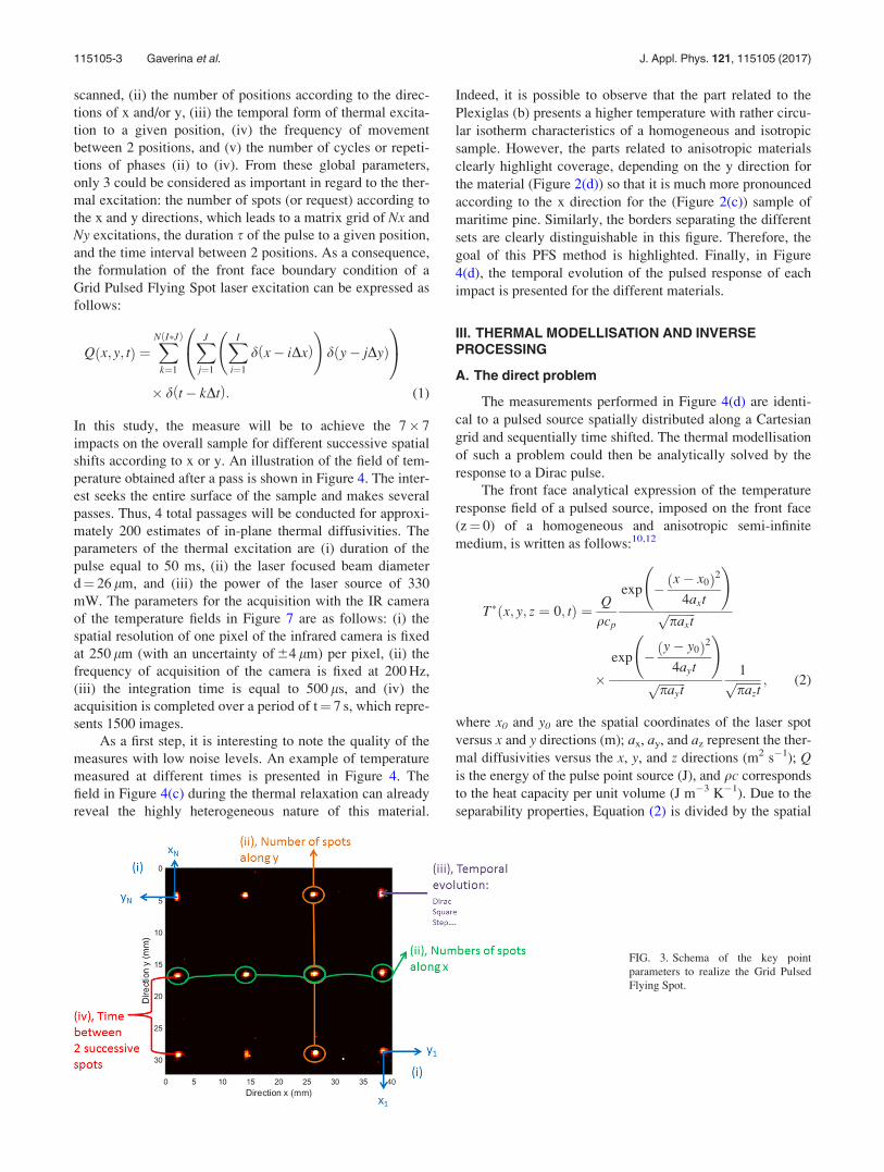
scanned, (ii) the number of positions according to the direc-

tions of x and/or y, (iii) the temporal form of thermal excita-

tion to a given position, (iv) the frequency of movement

between 2 positions, and (v) the number of cycles or repeti-

tions of phases (ii) to (iv). From these global parameters,

only 3 could be considered as important in regard to the ther-

mal excitation: the number of spots (or request) according to

the x and y directions, which leads to a matrix grid of Nx and

Ny excitations, the duration s of the pulse to a given position,

and the time interval between 2 positions. As a consequence,

the formulation of the front face boundary condition of a

Grid Pulsed Flying Spot laser excitation can be expressed as

follows:

Q x; y; tð Þ ¼XN I�Jð Þ

k¼1

XJ

j¼1

XI

i¼1

d x� iDxð Þ !

d y� jDyð Þ

0@

1A

� d t� kDtð Þ: (1)

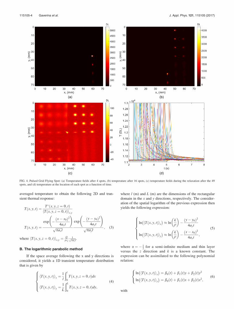
In this study, the measure will be to achieve the 7� 7

impacts on the overall sample for different successive spatial

shifts according to x or y. An illustration of the field of tem-

perature obtained after a pass is shown in Figure 4. The inter-

est seeks the entire surface of the sample and makes several

passes. Thus, 4 total passages will be conducted for approxi-

mately 200 estimates of in-plane thermal diffusivities. The

parameters of the thermal excitation are (i) duration of the

pulse equal to 50 ms, (ii) the laser focused beam diameter

d¼ 26 lm, and (iii) the power of the laser source of 330

mW. The parameters for the acquisition with the IR camera

of the temperature fields in Figure 7 are as follows: (i) the

spatial resolution of one pixel of the infrared camera is fixed

at 250 lm (with an uncertainty of 64 lm) per pixel, (ii) the

frequency of acquisition of the camera is fixed at 200 Hz,

(iii) the integration time is equal to 500 ls, and (iv) the

acquisition is completed over a period of t¼ 7 s, which repre-

sents 1500 images.

As a first step, it is interesting to note the quality of the

measures with low noise levels. An example of temperature

measured at different times is presented in Figure 4. The

field in Figure 4(c) during the thermal relaxation can already

reveal the highly heterogeneous nature of this material.

Indeed, it is possible to observe that the part related to the

Plexiglas (b) presents a higher temperature with rather circu-

lar isotherm characteristics of a homogeneous and isotropic

sample. However, the parts related to anisotropic materials

clearly highlight coverage, depending on the y direction for

the material (Figure 2(d)) so that it is much more pronounced

according to the x direction for the (Figure 2(c)) sample of

maritime pine. Similarly, the borders separating the different

sets are clearly distinguishable in this figure. Therefore, the

goal of this PFS method is highlighted. Finally, in Figure

4(d), the temporal evolution of the pulsed response of each

impact is presented for the different materials.

III. THERMAL MODELLISATION AND INVERSEPROCESSING

A. The direct problem

The measurements performed in Figure 4(d) are identi-

cal to a pulsed source spatially distributed along a Cartesian

grid and sequentially time shifted. The thermal modellisation

of such a problem could then be analytically solved by the

response to a Dirac pulse.

The front face analytical expression of the temperature

response field of a pulsed source, imposed on the front face

(z¼ 0) of a homogeneous and anisotropic semi-infinite

medium, is written as follows:10,12

T� x; y; z ¼ 0; tð Þ ¼ Q

qcp

exp �x� x0ð Þ2

4axt

!ffiffiffiffiffiffiffiffiffipaxtp

�exp �

y� y0ð Þ2

4ayt

!ffiffiffiffiffiffiffiffiffipaytp

1ffiffiffiffiffiffiffiffipaztp ; (2)

where x0 and y0 are the spatial coordinates of the laser spot

versus x and y directions (m); ax, ay, and az represent the ther-

mal diffusivities versus the x, y, and z directions (m2 s�1); Qis the energy of the pulse point source (J), and qc corresponds

to the heat capacity per unit volume (J m�3 K�1). Due to the

separability properties, Equation (2) is divided by the spatial

FIG. 3. Schema of the key point

parameters to realize the Grid Pulsed

Flying Spot.

115105-3 Gaverina et al. J. Appl. Phys. 121, 115105 (2017)

averaged temperature to obtain the following 2D and tran-

sient thermal response:

T x; y; tð Þ ¼T� x; y; z ¼ 0; tð ÞhT x; y; z ¼ 0; tð Þix;y

T x; y; tð Þ ¼exp �

x� x0ð Þ2

4axt

!ffiffiffiffiffiffiffiffiffipaxtp

exp �y� y0ð Þ2

4ayt

!ffiffiffiffiffiffiffiffiffipaytp ; (3)

where hT x; y; z ¼ 0; tð Þix;y ¼Q

qcp

1ffiffiffiffiffiffipaztp .

B. The logarithmic parabolic method

If the space average following the x and y directions is

considered, it yields a 1D transient temperature distribution

that is given by

hT x; y; tð Þix ¼1

l

ðl

0

T x; y; z ¼ 0; tð Þdx

hT x; y; tð Þiy ¼1

L

ðL

0

T x; y; z ¼ 0; tð Þdy;

8>>><>>>:

(4)

where l (m) and L (m) are the dimensions of the rectangular

domain in the x and y directions, respectively. The consider-

ation of the spatial logarithm of the previous expression then

yields the following expression:

ln hT x; y; tð Þix� �

� lnk

ta

� ��

y� y0ð Þ2

4ayt

ln hT x; y; tð Þiy� �

� lnk

ta

� ��

x� x0ð Þ2

4axt;

8>>>><>>>>:

(5)

where a ¼ � 12

for a semi-infinite medium and thin layer

versus the z direction and k is a known constant. The

expression can be assimilated to the following polynomial

relation:

ln hT x; y; tð Þix� �

¼ b0 tð Þ þ b1 tð Þyþ b2 tð Þy2

ln hT x; y; tð Þiy� �

¼ b0 tð Þ þ b1 tð Þxþ b2 tð Þx2;

8<: (6)

with

FIG. 4. Pulsed Grid Flying Spot: (a) Temperature fields after 4 spots, (b) temperature after 16 spots, (c) temperature fields during the relaxation after the 49

spots, and (d) temperature at the location of each spot as a function of time.

115105-4 Gaverina et al. J. Appl. Phys. 121, 115105 (2017)

b2 tð Þ¼� 1

4axtor� 1

4ayt

b1 tð Þ¼ x0

2axtor

y0

2aytor� 1

2b2 tð Þ¼x0

b1 tð Þor� 1

2b2 tð Þ¼y0

b1 tð Þ

b0 tð Þ¼� x02

4axtþ ln

k

ta

� �or� y0

2

4aytþ ln

k

ta

� � :

8>>>>>>>><>>>>>>>>:

(7)

Several comments arise from the previous expressions:

• b2 tð Þ is dependent only on the thermal diffusivities ax and

ay. It is thus a suitable way to verify the in-plane homoge-

nous transfer at different time steps, independent of the

transverse heat transfer and the position of the spot.• When the in-plane thermal diffusivities were estimated

using b2 tð Þ, the estimation of x0 and y0 could be conducted

with the b1 tð Þ parameter or with the direct relation

between b1 tð Þ and b2 tð Þ.• The estimation of b0 tð Þ is directly related to a 1D front

face flash experiment; this type of signal contributes to the

process. For example, the TSR method6 could be used to

estimate the parameter on an ln(T) versus ln(t) graph

representation.

C. The inverse processing

For convenience, the measurement noise is considered

uniform on the distribution and expressed as follows:

T_

x; y; tið Þ ¼ T x; y; tið Þ þ eT x;y;tið Þ; (8)

where eT x;y;tið Þ is the random fluctuation added to a signal

T x; y; tið Þ. It is considered to have a zero mean and uniform

standard deviation (the covariance matrix is diagonal).

The space average of Equation (7) is given by

�Tn ¼ �Tn þ e �T n; (9)

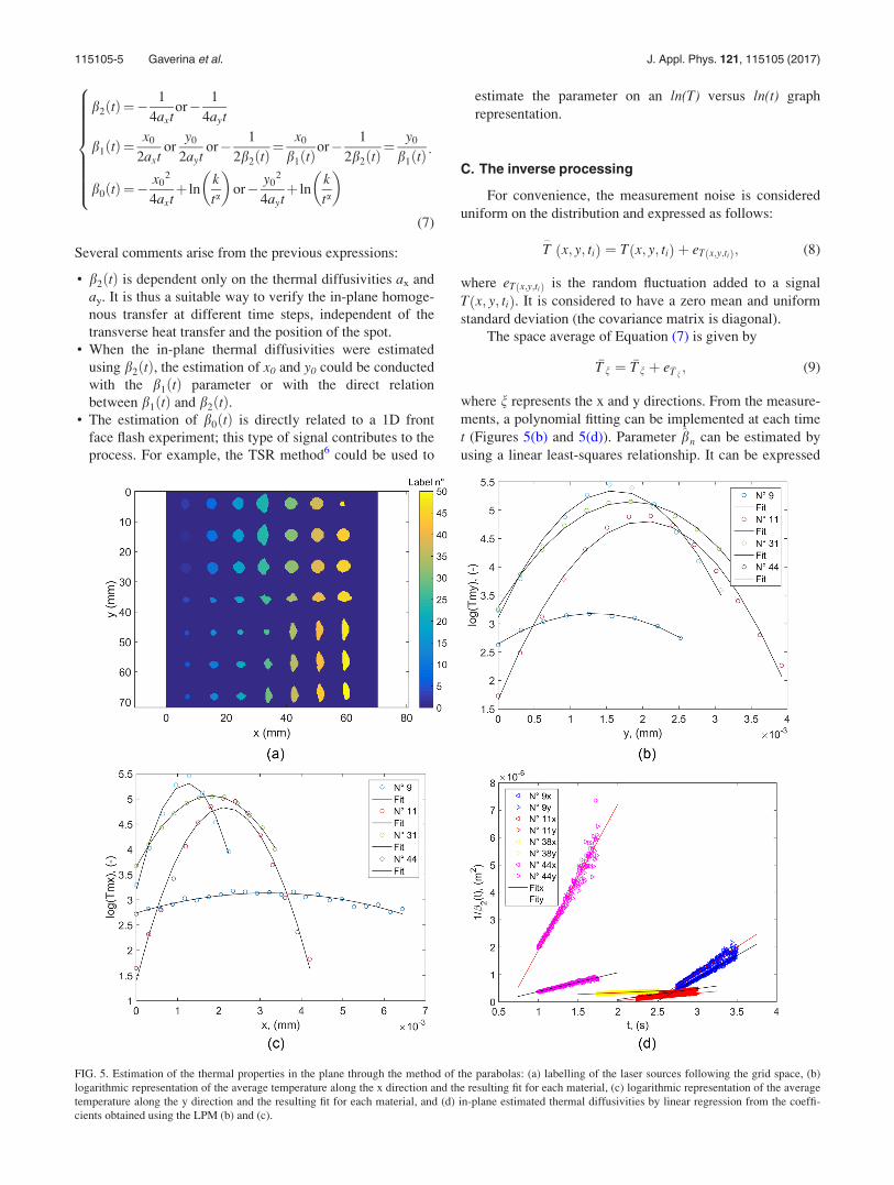
where n represents the x and y directions. From the measure-

ments, a polynomial fitting can be implemented at each time

t (Figures 5(b) and 5(d)). Parameter bn can be estimated by

using a linear least-squares relationship. It can be expressed

FIG. 5. Estimation of the thermal properties in the plane through the method of the parabolas: (a) labelling of the laser sources following the grid space, (b)

logarithmic representation of the average temperature along the x direction and the resulting fit for each material, (c) logarithmic representation of the average

temperature along the y direction and the resulting fit for each material, and (d) in-plane estimated thermal diffusivities by linear regression from the coeffi-

cients obtained using the LPM (b) and (c).

115105-5 Gaverina et al. J. Appl. Phys. 121, 115105 (2017)

as a linear combination of the logarithm of the measured

temperature ln �Tn

� �with a parameter such that ln �Tn

� �¼ S � b, where S is the sensitivity matrix.

ln �Tn1

� �...

ln �TnN

� �

26664

37775 ¼

1 n1 n12

..

. ... ..

.

1 nN nN2

264

375: (10)

The method of least squares assumes that there is constant var-

iance in the noise, but in this case, the method of weighted

least squares (Equation (11)) must be used because the ordi-

nary least squares assumption of constant variance in the noise

is violated (heteroscedasticity), as shown in Equation (10)

ln �T n

� �¼ ln �T n

� �þ

e �T n

�Tn: (11)

The optimal estimation then yields:

b ¼ STWSð Þ�1STW ln �T n

� �; (12)

where W is given by the diagonal elements of the variance–

covariance matrix in the noise.

IV. EXPERIMENTAL RESULTS AND DISCUSSION OFHETEROGENEOUS AND ANISOTROPIC MATERIALS

The results presented in this section come from the set

of experiments illustrated in Figure 4 and based on the GPFS

technique described in Section II associated with the LPM.

From the previous theoretical considerations, it is necessary

to validate the different steps of the parameter estimation

shown in Equation (6). First, as known by IR thermography,

the offset due to the surroundings is subtracted from all the

acquired images. From one set of experiments (as shown in

Figure 2), a threshold method13–15 is used to mark the centre

of each laser spot, as shown in Figure 5(a).

From this location, the two marginal averages of

Equation (4) are calculated as functions of time. To optimize

the area where the parabolic fit of Equation (6) is performed,

the spatial first-order derivative of the marginal averages is

calculated for both the directions. The detection of the maxi-

mum and the minimum of this derivative allows the optimal

zone for the parabolic fitting to be defined. Inside this opti-

mal area, quadratic fits (Equation (12)) are realized for the

several sub-materials and illustrated in Figures 5(b) and 5(c).

From these fits, the 3 coefficients of the polynomial of order

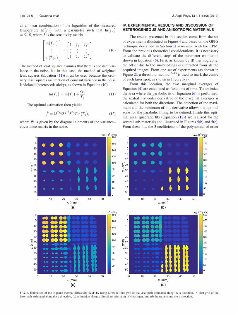
FIG. 6. Estimation of the in-plane thermal diffusivity fields by using LPM: (a) first grid of the laser path estimated along the x direction, (b) first grid of the

laser path estimated along the y direction, (c) estimation along x directions after a set of 4 passages, and (d) the same along the y direction.

115105-6 Gaverina et al. J. Appl. Phys. 121, 115105 (2017)

2 are estimated for each time step and for each of the differ-

ent impacts of the laser source. By using the linear fit from

Equation (7), the thermal diffusivities and the location of the

laser spot can be retrieved (see Figure 5(d)). These slopes

according to Equation (7) are directly proportional to the

thermal diffusivities. To avoid errors in estimating the ther-

mal diffusivity and the laser location, the best estimation

corresponds to the thermal relaxation, where the linear

behaviour is observed with a high signal-to-noise ratio. Over

a short time, the estimation is biased because the specimen is

illuminated by a Gaussian laser beam of radius R.10,11,17,18

Thus, the y-intercept of this curve is proportional to the

radius of the beam laser instead of being equal to zero as pre-

dicted by using the model Equation (2) of a Dirac spatial

pulse.

First, to validate the measured data in the case of homo-

geneous isotropic and anisotropic samples, particular atten-

tion is paid to the results of the estimation of sub-samples b

and d (see Figure 4) for which the data are given in the litera-

ture.16,19 The estimated in-plane thermal diffusivities (Figure

5(d)) of the Plexiglass sample (Figure 4(b)) are ax¼ 1.1

� 10�7 m2 s�1 and ay¼ 1.13� 10�7 m2 s�1. These values

are in good agreement with a¼ 1.09� 10�7 m2 s�1 given by

Ref. 16 with a difference of less than 2%. Moreover, the

very low difference between ax and ay confirms the isotropy

of the sample. Concerning the sample of carbon/epoxy

(Figure 4(d)), the estimated values by using Equation (6) of

the in-plane thermal diffusivities (Figure 5(d)) are ax

¼ 6.74� 10�7 m2 s�1 and ay¼ 5.44� 10�6 m2 s�1. These

values confirm the anisotropic assumption of the sample

with a calculated ratio of ay to ax of 8. This behaviour is in

very good agreement with the values of the thermal diffusiv-

ity found in the literature19 with respective differences of

1.92% in the x direction and 3.45% in the y direction. These

results allow us to validate the method to realize the com-

plete thermal characterization of the heterogeneous sample

in Figure 4. For that, this procedure is illustrated in Figures

6(a) and 6(b) in the case of a single path and then generalized

to Figures 6(c) and 6(d) for 4 paths. Here, it should be noted

that after 4 successive paths, each material has been esti-

mated approximately 36 times on its entire surface.

These results clearly show the relevance of the tool

(methods and measures) developed in this work. In addition,

the chosen example (heterogeneous anisotropic material)

also highlights the ability of this approach to quantitatively

characterize a field of thermal diffusivities in the plan. It

should be noted that the anisotropic character is well found

and identified for sub-materials a, c, and d. Finally, “cracks”

that voluntarily left spaces during the assembly of these 4

under-materials are also identified. Finally, from this set of

measures, it is possible to refine the mesh or grid of scanning

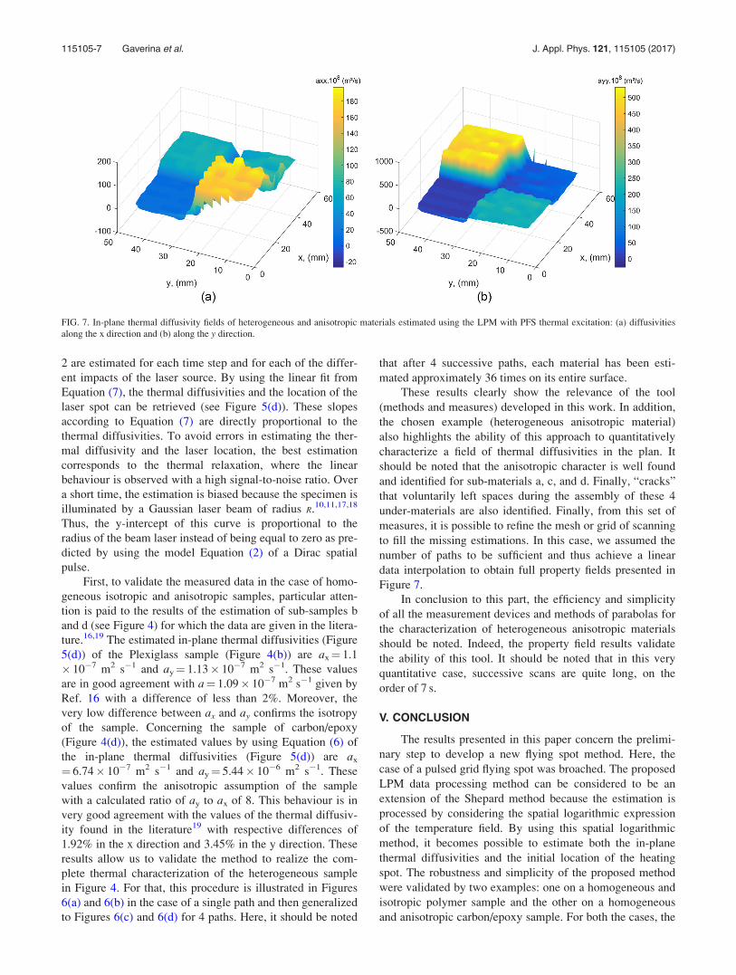
to fill the missing estimations. In this case, we assumed the

number of paths to be sufficient and thus achieve a linear

data interpolation to obtain full property fields presented in

Figure 7.

In conclusion to this part, the efficiency and simplicity

of all the measurement devices and methods of parabolas for

the characterization of heterogeneous anisotropic materials

should be noted. Indeed, the property field results validate

the ability of this tool. It should be noted that in this very

quantitative case, successive scans are quite long, on the

order of 7 s.

V. CONCLUSION

The results presented in this paper concern the prelimi-

nary step to develop a new flying spot method. Here, the

case of a pulsed grid flying spot was broached. The proposed

LPM data processing method can be considered to be an

extension of the Shepard method because the estimation is

processed by considering the spatial logarithmic expression

of the temperature field. By using this spatial logarithmic

method, it becomes possible to estimate both the in-plane

thermal diffusivities and the initial location of the heating

spot. The robustness and simplicity of the proposed method

were validated by two examples: one on a homogeneous and

isotropic polymer sample and the other on a homogeneous

and anisotropic carbon/epoxy sample. For both the cases, the

FIG. 7. In-plane thermal diffusivity fields of heterogeneous and anisotropic materials estimated using the LPM with PFS thermal excitation: (a) diffusivities

along the x direction and (b) along the y direction.

115105-7 Gaverina et al. J. Appl. Phys. 121, 115105 (2017)

retrieved results of the in-plane thermal diffusivities are in

very good agreement with those of the literature (error lower

than 4%). The entire processing was then applied to a hetero-

geneous and anisotropic sample. The obtained results show

the ability to obtain full fields of in-plane thermal properties.

Finally, this easy-to-implement method can be considered to

be a new tool for the in-plane thermal characterization of

materials. It should be noted that when the materials become

too conductive, the estimation method still remains valid. On

the other hand, it is necessary to use heterodyne methods for

the acquisition.20 In the future, polynomial development can

be considered at higher orders for the detection of cracks per-

pendicular or parallel to the observation surface, mapping of

thermophysical properties, and research of a small anomaly

over a large area by using the pulsed flying spot technique.

ACKNOWLEDGMENTS

This work was supported by “Projet R�egion Aquitaine”

and “Epsilon-Alcen” Industrial Groups.

1J. Krapez, L. Legrandjacques, F. Lepoutre, and D. Balageas,

“Optimization of the photothermal camera for crack detection,” in

Proceedings of QIRT98 Conference (Seminar Eurotherm No 60), edited

by D. Balageas, G. Busse, and G. M. Carlomagno (Akademickie Centrum

Graficzno-Marketingowe Lodart SA, Ldz, Poland, 1998), Vol. 25, pp.

305–310; See www.qirt.org/dynamique/index.php?idD¼55 for A QIRT

Open Archives, Paper No. QIRT 1998-048.2C. Gruss and D. Balageas, “Theoretical and experimental applications of

the flying spot camera,” in Proceedings of QIRT 92 Conference (SeminarEurotherm No 27), edited by D. Balageas, G. Busse, and G. M.

Carlomagno (Editions Europennes Thermique et Industrie, Paris, 1992),

pp. 19–24; See www.qirt.org/dynamique/index.php?idD¼55 for QIRT

Open Archives, Paper No. QIRT 1992-004.3Y. Wang, P. Kuo, L. Favro, and R. Thomas, “A novel flying-spot infrared

camera for imaging very fast thermal-wave phenomena,” in Photoacousticand Photothermal Phenomena II, Springer Series in Optical Sciences

(Springer, 1990), pp. 24–26.4T. Li, D. P. Almond, and D. A. S. Rees, “Crack imaging by scanning

pulsed laser spot thermography,” NDT & E Int. 44(2), 216–225 (2011).5J. C. Krapez, “Spatial resolution of the flying spot camera with respect to

cracks and optical variations,” in Proceedings of the 10th InternationalConference on Photoacoustic and Photothermal Phenomena (1999), Vol.

463, pp. 377–379.

6S. Shepard and M. Frendberg, “Thermographic detection and characteriza-

tion of flaws in composite materials,” Mater. Eval. 72(7), 928 (2014).7I. Philippi, J., Batsale, D. Maillet, and A. Degiovanni, “Measurement of

thermal diffusivities through processing of infrared images,” Rev. Sci.

Instrum. 66(1), 182–192 (1995).8J. C. Krapez, L. Spagnolo, M. Frieß, H. P. Maier, and G. Neuer,

“Measurement of in-plane diffusivity in non-homogeneous slabs by

applying flash thermography,” Int. J. Thermal Sci. 43(10), 967–977

(2004).9M. Bamford, M. Florian, G. L. Vignoles, J. C. Batsale, C. A. A. Cairo, and

L. Maill�e, “Global and local characterization of the thermal diffusivities of

sic f/sic composites with infrared thermogra- phy and flash method,”

Compos. Sci. Technol. 69(7), 1131–1141 (2009).10F. Cernuschi, A. Russo, L. Lorenzoni, and A. Figari, “In-plane thermal dif-

fusivity evaluation by infrared thermography,” Rev. Sci. Instrum. 72(10),

3988–3995 (2001).11P. Bison, F. Cernuschi, and S. Capelli, “A thermographic technique for the

simultaneous estimation of in-plane and in-depth thermal diffusivities of

tbcs,” Surf. Coat. Technol. 205(10), 3128–3133 (2011).12H. S. Carslaw and J. C. Jaeger, Conduction of Heat in Solids, 2nd ed.

(Clarendon Press, Oxford, 1959).13M. Bamford and J. C. Batsale, “Analytical singular value decomposition

of infrared image sequences: Microcrack detection on ceramic composites

under mechanical stresses,” C. R. M�ec. 336(5), 440–447 (2008).14C. Pradere, J. Morikawa, J. Toutain, J. C. Batsale, E. Hayakawa, and T.

Hashimoto, “Microscale thermography of freezing biological cells in view

of cryopreservation,” Quant. Infrared Thermogr. J. 6(1), 37–61 (2009).15J. C. Batsale and C. Pradere, “Infrared image processing devoted to ther-

mal non-contact characterization-applications to non-destructive evalua-

tion, microfluidics and 2d source term distribution for multispectral

tomography,” J. Phys.: Conf. Ser. 655(1), 012002 (2015).16A. L. Edwards, “A compilation of thermal property data for computer

heat-conduction calculations,” Report No. UCRL-50589, University of

California Lawrence Radiation Laboratory, 1969.17N. W. Pech-May, A. Mendioroz, and A. Salazar, “Simultaneous measure-

ment of the in-plane and in-depth thermal diffusivity of solids using pulsed

infrared thermography with focused illumination,” NDT & E Int. 77,

28–34 (2016).18A. Degiovanni, “Correction de longueur d’impulsion pour la mesure de la

diffusivit�e thermique par m�ethode flash,” Int. J. Heat Mass Transfer

30(10), 2199–2200 (1987).19M. Thomas, N. Boyard, N. Lefevre, Y. Jarny, and D. Delaunay, “An

experimental device for the simultaneous estimation of the thermal con-

ductivity 3-D tensor and the specific heat of orthotropic composite materi-

als,” Int. J. Heat Mass Transfer 53(23), 5487–5498 (2010).20C. Pradere, L. Clerjaud, J. C. Batsale, and S. Dilhaire, “High speed hetero-

dyne infrared thermography applied to thermal diffusivity identification,”

Rev. Sci. Instrum. 82, 054901 (2011), ISSN: 0034-6748.

115105-8 Gaverina et al. J. Appl. Phys. 121, 115105 (2017)