.v 7

,

Pulse Shaping Techniques for Testing Brittle Materials with a SplitHopkinson Pressure Bar

by D. J. Frew, M. J. Fomestal and W. Chen

ABSTRACT- We present pulse shaping techniques to

brittle materials with the split Hopkinson pressure.

obtain compressive stress-strain data for

bar apparatus. The conventional split

Hopkinson pressure bar apparatus is modified by shaping the incident pulse such that the

samples are in dynamic stress equilibrium and have nearly constant strain rate over most of the

test duration. A’thin disk of annealed or hard C 11000 copper is placed on the impact surface of

the incident bar in order to shape the incident pulse. After impact by the striker bar, the copper

disk deforms plastically and spreads the pulse in the incident bar. We present an analytical

model and data that show a wide variety of incident strain pulses can be produced by varying the

geometry of the copper disks and the length and striking velocity of the striker bar. Model

predictions are in good agreement with measurements. In addition, we present data for a

machinable glass ceramic material, Macor, that shows pulse shaping is required to obtain

dynamic stress equilibrium and nearly constant strain rate over most of the test duration.

D. J Frew is Research Engineer, USAERDC Waterways Experiment Station, Vicksburg, M’S 39180-6199. M JForrestal (SEM Member) is Distinguished Member of Technical Stafl Sandia National Laboratories, Albuquerque,NM 87185-0303. W. Chen (SEM Member) is Assistant Professor, Department of A erospace and MechanicalEngineering, The University of Arizona, Tucson, AZ 85721-0119.

1

DISCLAIMER

This report was prepared as an account of work sponsoredby an agency of the United States Government. Neitherthe United States Government nor any agency thereof, norany of their employees, make any warranty, express orimplied, or assumes any legal liability or responsibility forthe accuracy, completeness, or usefulness of anyinformation, apparatus, product, or process disclosed, orrepresents that its use would not infringe privately ownedrights. Reference herein to any specific commercialproduct, process, or service by trade name, trademark,manufacturer, or otherwise does not necessarily constituteor imply its endorsement, recommendation, or favoring bythe United States Government or any agency thereof. Theviews and opinions of authors expressed herein do notnecessarily state or reflect those of the United StatesGovernment or any agency thereof.

DISCLAIMER

Portions of this document may be illegiblein electronic image products. Images areproduced from the best available originaldocument.

IntroductionF/ml 15 2Mlo

CMiimThe split Hopkinson pressure bar (SHPB) technique originally developed by Kolsky[} 2

has been used by many investigators to obtain dynamic compression properties of solid

materials. The evolution of this experimental method and recent advances are discussed by

Nicholas3, Nemat-Nasser, Isaacs, and Starrett4, Ramesh and Narasimhan5, Gray6, and Gray and

Blumenthal.’ This technique has mostly been used to study the plastic flow stress of metals that

undergo large strains at strain rates between 102 – 104s-1. As discussed 6y Yadav, Chichili, and

Rarneshg, data for the compressive flow stress of metals are typically obtained for strains larger

than a few percent because the technique is not capable of measuring the elastic and early yield

behavior. By contrast, most of the material behavior of interest for relatively brittle materials

such as ceramics and rocks occurs at strains less than about 1.0 percent.

For an ideal Kolsky compression bar experiment, the sample should be in dynamic stress

equilibrium and deform at a nearly constant strain rate over most of the test duration. To

approximate these ideal conditions for brittle ceramic materials, Nemat-Nasser, Isaacs, and

Starrett4 modified the conventional Kolsky compression bar by placing an oxygen-free-copper

(OFHC) disk on the impact surface of the incident bar. When the striker bar impacts the copper

disk, the large plastic deformation of the disk spreads the pulse in

time for the ceramic sample to achieve dynamic stress equilibrium.

the incident bar is an essential modification for testing ceramics with

the incident bar and allows

Thus, shaping the pulse in

the compression Kolsky bar

technique. Experiments that attempt to obtain high-rate, stress-strain data for ceramic materials

at constant strain rates are reported by Rogers and Nemat-Nasser9 and Chen and Ravichandran. *0

In addition, Nemat-Nasser, Isaacs, and Starrett4 present a model that predicts the strain pulse in

the incident bar for an OFHC copper pulse shaper, and Ravichandran and Subashl’ present a

,. ~

sample equilibrium model for ceramic materials. More recently, Frew, Forrestal, and Chen12

extended this work4> ‘‘ to obtain high-rate, stress-strain data for limestone samples. Data from

experiments with limestone samples showed that the samples were in dynamic stress equilibrium

and had nearly constant strain rates over most the test durations for a ramp pulse in the incident

bar.

While pulse shaping techniques have been successfully used to achieve the goals of many

different experiments, pulse shapers are usually designed by experimental trials that exclude a

model to guide the design parameters. For example, Duffy, Campbell, and Hawley13 used a

pulse shaper to smooth pulses generated by explosive loading for torsional Hopkinson bar

experiments, and Wu and Gorham’4 used paper on the impact surface of the incident bar to

eliminate high

experiments.

frequency oscillations in the incident pulse for Kolsky

Togami, Baker, and Forrestal’5 used a thin, plexiglass

nondispersive compression pulses in an incident bar, and Chen, Zhang, and

compression bar

disk to produce

Forresta116 used a

polymer disk to spread the incident compressive pulses for experiments with elastomers.

Christensen, Swanson, and Brown17 used striker bars with a truncated-cone on the impact end in

an attempt to produce ramp pulses. In contrast to other pulse shaping studies, Nemat-Nasser,

Isaacs, and Starrett4 model the plastic deformation of an OFHC copper pulse shaper, predict the

incident strain pulse, and show good agreement with some measured incident strain pulses.

In this study, we extend the analytical model of Nemat-Nasser, Isaacs, and Starrett4 and

present new data for annealed and hard C 1100018 copper pulse shapers. Experiments conducted

with both OFHC and C 11000 copper pulse shapers showed a superior performance by the

C 11000 materials. In particular, the C 11000 pulse shapers could be dfiven to larger strains

without breakup or fracture and remained more circular after deformation. We found that with

3

. < ,c

both annealed and hard Cl 1000 pulse shapers, we could obtain a broad range of strain rates for

testing brittle ceramic and rock*2 materials. The previous mode14 was extended to accommodate

the large strains obtained in the C 11000 copper materials. In addition, we present data for the

ceramic material Macorlg that shows pulse shaping is required to obtain dynamic stress

equilibrium and nearly constant strain rate over most of the test duration.

Split Hopkinson Pressure Bar (SHPB) or Kolsky Bar

As shown in Fig. 1,

striker bar, an incident bar,

a conventional split Hopkinson pressure bar (SHPB) consists of a

a transmission bar, and a sample placed between the incident and

transmission bars. A gas gun launches the striker bar at the incident bar and that impact causes

an elastic compression wave to travel in the incident bar towards the sample. When the

impedance of the sample is less than that of the bars, an elastic tensile wave is reflected into the

incident bar and an elastic compression wave is transmitted into the transmission bar. If the

elastic stress pulses in the bars are nondispersive and the specimen deforms with homogeneous

deformation, the elementary theory for wave propagation in bars can be used to calculate the

sample response from measurements taken with strain gages mounted on the incident and

transmission bars. Strain gages mounted on the incident bar measure the incident &iand reflected

s~ strain pulses, and strain gages mounted on the transmission bar measure the transmitted St

strain pulse. Nicholas3, and Gray6 present equations that describe the sample response in terms

of the measured strain signals.

For this study the incident and transmission bars were made from the same material with

equal cross-sectional areas. As shown in Fig. 1, the bars have density p, Young’s modulus E, bar

wave speed c, and cross-sectional area A. Since we only focus on brittle materials that have

4

failure strains less than about 1.0 percent, we need only use engineering stress, strain, and strain-

rate measures. In addition, we take stress positive in compression, strain positive in contraction,

and particle velocity positive to the right in Fig. 1. Figure 1 also shows the sample has cross-

sectional area AS and length L. We take subscripts 1 and 2 to represent the locations of the ends

of the sample.

From Nicholas3

If crl = OZ, the stresses

(la)

(lb)

on both ends of the sample are equal, the sample is in dynamic stress

equilibrium, and the stress, strain rate, and strain are given by

EAc7s=—

A, “

dq –2CE—=—dt 10 ‘

&s ‘+j’6,(.) d.,0 0

(2)

(3)

(4)

As discussed in detail by Ravichandran and Subash* *, Gray6, and Gray and Blumenthal,

5

. ~c

eqs (2), (3), and (4) assume that the sample is in dynamic stress equilibrium. Equilibrium should

Ifirst be examined by comparing the stresses crl and cr2at the ends of the sample given by eqs (1a)

and (1b). If 01 and cr2are in reasonable agreement, only then it is reasonable to use eqs (2), (3),

Iand (4) to calculate sample stress, strain rate, and strain.

Models for Sample Equilibrium and Constant Strain Rate

In a recent paper*2, we presented models that predict the evolutionary process for sample

equilibrium and constant strain rate for brittle materials that have a linear stress-strain response

until failure. These models were limited to a ramp stress pulse in the incident bar and provided

valueable experimental design information for limestone samples. In our more recent work with

brittle materials, we learned that it was relatively easy to obtain sample equilibrium and more

difficult to obtain a nearly constant strain rate over most of the test duration. To assist our

experimental design procedures prior to testing, we extend our previous models] 2 to include a

general incident stress pulse. The more general models allow us to examine incident pulses that

produce nearly constant strain rates in the sample for a broader range of strain rates. The first

model assumes that the sample is in dynamic stress equilibrium and predicts strain and strain rate

versus time. For the second model, we perform a wave propagation analysis on the interaction of

the sample with the incident and transmission bars. This second model predicts the stress-time

histories on either side of the sample.

From the derivations in Frew, Forrestal, and Chen]2, sample strain is governed by the

differential equation

(5)

where the sample has the linear stress-strain relation

and ~i(t) is the incident pulse at the incident bar/ sample interface. For a polynomial incident

stress

~i(t) =CTo +Mt + Nt2

equation (5) has solutions

-.*exp(”]+ &[l-exp(+)]+ds,

dt

W-’+:+exp(al

‘s=%[’-expHl+fH-expHz, [ H+’[++=qW(%)* ~+

Apcy=:, r= to J%AS P, c, ‘s c,

7

(7)

(8a)

(8b)

(8c)

Equations (8a) and (8b) give closed-form solutions for the strain rate and strain in the sample..

However, this model assumes that the sample is in equilibrium.

For the second model, we perform a wave propagation analysis on the interaction of the

sample with the incident and transmission bars. Following the procedure developed by Frew,

Forrestal, and Chen12, the stresses in the sample at interface 1 shown in Fig. 1 are

(7,=~ai(t),r+l

O< t < 2t0 (9a)

4t0 s t < 6t0 (9c)

and that at interface 2 are

02 = 0, O<t < tO (lOa)

[012y ~+ r–102. — — Oi(t– to)

r+l r+lto < t < 3t0 (lOb)

8

The nth term for eqs (9) and (10) is

where tO is given by eq (8c) and corresponds to one wave travel time

Therefore, al and 02 can easily be calculated for times greater than those

(10). We later show predictions from

for glass ceramic Macorlg material.

forntO <t< (n +2)t0,

through the sample.

given by eqs (9) and

these models and measured stress and strain-rate histories

Pulse Shaping

As previously discussed, the conventional split Hopklnson pressure bar apparatus is

modified by shaping the incident pulse such that the samples are in dynamic stress equilibrium

and have nearly constant strain rate over most of the test duration. To achieve these ideal test

conditions for brittle materials, we extend the work of Nemat-Nasser, Isaacs, and Starrett4 who

used an OFHC copper disk on the impact surface of the incident bar to shape the incident pulse.

In this study, we conducted experiments with both OFHC and Cl 1000*8 copper pulse shapers

and showed a superior performance by the C 11000 materials. In particular, the C 11000 pulse

shapers could be driven to larger strains without breakup or fracture and remained more circular

after deformation. We found that with both annealed and hard C 11000 pulse shapers, we could

obtain a broad range of strain rates for testing brittle ceramic and rock]2 materials. The previous

mode14 was extended to accommodate the large strains obtained with the C 11000 copper pulse

9

I

.

shaper materials. In addition, remodified the equations that govern wave propagation in the

striker bar to incorporate the added mass from the sabot and included elastic, rather than rigid,

unloading in the pulse shaping analysis. Incident pulse model predictions are shown to be in

good agreement with strain measurements.

Figure 2a shows a schematic of the impact end of the SHPB apparatus with a pulse

shaper that is attached with a light coating of grease. In Fig. 2a, p,~, c,~, and A are the density,

bar wave velocity, and cross-sectional area of the striker bar, respectively; V. is the striker bar

velocity at impact; and % and b are the initial cross-sectional area and thickness of the pulse

shaper. When the striker bar impacts the pulse shaper, compressive forces are gradually

transferred from the pulse shaper to the incident bar. The deformation of the pulse shaper

increases its load carrying capacity by

hardening of the pulse shaping material.

load carrying capacity of the pulse shaper

increasing its cross-sectional area and by the strain

As will be shown later, the monotonic increase of the

causes longer duration pulses in the incident bar.

pulse Shaping Model

For an incompressible material and a homogeneous deformation, mass conservation gives

aOhO= a(t)h(t), (11)

where a(t) and h(t) are the current cross-sectional area and thickness of the pulse shaper. The

axial engineering strain in the pulse shaper is given by

10

.

hO - h(t)&p(t) = = 1 h(t)

hO hO(12)

which is positive in contraction. From eqs (11) and (12), the current cross-sectional area of the

pulse shaper can be written in terms of the original area and axial strain in the pulse shaper.

Thus,

a(t) = aol-&p(t)”

(13)

The axial force exerted by the pulse shaper on the ends of the striker and incident bars is

T(t) = o, (t)a(t) = o, (t)A = o,, (t)A, (14)

where aP(t) is the true axial stress in the pulse shaper, ~l(t) is from the compressive stress wave

traveling to the right in the incident bar, and a,~(t) is from the compressive stress wave traveling

to the left in the striker bar. From eq (14), the bar stresses at the pulse shaper/ bar interfaces are

Op (t)a(t)ai (t) = 0,, (t) = A . (15)

For now, let ~P(t) be defined by the general. form of a one-dimensional stress-strain relationship

where GOis a constant and g(cP) is a function of the pulse shaper engineering axial strain. From

eqs (12), (15), and (16)

00a. g(&p)‘i (t)= ‘N (t) = —

A (1–6,)”(17a)

Since the incident and striker bars remain elastic, the axial strains in the bars at the bar/ pulse

shaper interfaces can be written as

00a. g(sp)‘i (t) = g,, (t)= —

EA (l–sP)”

The engineering strain rate in the pulse shaper is given by

v3(t) – v4(t)&p (t) =

hO ‘

(17b)

(18)

where v~(t) and v~(t) are the particle velocities at the striker bar/pulse shaper (3) and incident bar/

pulse shaper (4) interfaces, respectively shown in Fig. 2b. From the equations that relate stress

and particle velocity in the bars, v~(t) and v~(t) are given by

(Ti(t)v3(t)=vo –v,t(t)=vo– —

Pstc,,(19a)

12

ai (t)‘4(t) = ‘i(t) = —

pc ‘(19b)

where v~t(t) and vi(t) are the particle velocities in the striker and incident bars. As shown in

Figs. 1, and 2, the bar areas are equal. However, the striker bar is supported by a nylon sabot

that fits into the gun barrel. As will be shown later, this sabot mass must be included in the wave...’

analysis for the striker bar. Thus, the density and wave speed for the striker bar are denoted as

pst and c,t, respectively.

From eqs (14), (18), and (19)

[111 /3(s, )~~P(t) =1–K — — —, for OSt<r

pc + p,,c,t 1–Sp(20)

o

which has a solution

‘=Hl”K[++aa’dx3f0‘21a)

K=-2L

, and r=—AVO cSt

(21b)

where ~ is equal to two wave transit times in the striker bar. Once sP(t) is calculated from eq

(21a), the strain in the incident bar can be obtained fromeq(17b). In addition, eq (2 la) is valid

only as long as the pulse shaper does not expand beyond the bar surfaces. Equation (13) shows

13

that the engineering strain in the pulse shaper is limited for a given initial pulse shaper area %,

such that a(t) <A.

Equation (2 la) does not explicitly give values for strain in the pulse shaper as a fhnction

of time for O < t < ~. However, we can obtain closed-form equations for some of the features of

the SPversus t curve. For small enough values of GP,the second term in eq (20) can be neglected

and

V. ti5p=— fort<<l

hO(22a)

Also, the integral in eq (21a) must remain positive because time is always positive. Thus, the

largest value of strain in the pulse shaper &P~is given by

g(spm) 1

[- 1(l-&pm)=K 1 + 1 “

Pc Pstcst

From eqs (17a) and (22b) the maximum possible stress in the incident bar is given by

V.aim =

[- 11+1”

Pe Pstcst

(22b)

(22C)

Equation (22c) gives the value of incident stress for the problem without a pulse shaper. So if

14

the striker bar is long enough, the stress in the incident bar will approach but not exceed oi~

given by (22c).

We now examine the pulse shaper response for ~ < t < 2T. At t = ~ /2, the compressive

wave traveling to the left in the striker bar shown in Fig. 2b reaches the free surface and reflects

as a tensile pulse traveling to the right. At t =

striker bar/ pulse shaper interface and causes.

propagate in the striker and incident bars. We

~, this right traveling tensile pulse reaches the

additional reflected and transmitted waves to

define a,t(t-~) as the interface stress from the

right traveling tensile pulse. The additional reflected and transmitted interface stresses are

defined as ~,’(t-~) and ot’(t-~), respectively. Thus, the axial force in the pulse shaper is given by

T(t) = a, (t)a(t) = [a, (t) + o,’ (t - r)]A (23)

= [a,, (t) - c,, (t - r)+ o,’ (t - T)]A.

Particle velocities at the pulse shaper/ bar interfaces shown in Fig. 2b are

v3(t) = V. –V,t(t) –V,t(t –r)–vr’(t –~) (24a)

~st(t) ~,t(t – r) _ cTrl(t– r)=vo -—--PstCst P,,Cst PstCst

(Ti(t)+ CTt](t– 2-)‘l(t)=vi(t)+v~’(t–~)=—pc pc

(24b)

From eqs (1 8), (23), and (24), the engineering strain rate is

15

O,t(t) O,t (t- r)_ q’ (t- r) Oi (t) q’ (t- r).h03P(t) = VO-—-

Pstc,, PstCst Pstest P c P c

Now, we solve for ~,[(t-z) from eq (23) and eliminate o,l(t-~) from eq (25). Thus,

[

11-hOgP(t) =VO– —+—

Pc Pstcst -

From eqs (23), (16), and (13), the stress in the incident bar is

OP(t)a(t) crOg(&P)aOOi(t)+ot’(t–r) =

A = (l-&p) I

and from eq (17a)

~og(gp(t – ~)) a.0,,(t– r) =

(l-&p (t-r)) 1“

(25)

(26)

(27)

Finally, we substitute eqs (27) and (28) into eq (26) and obtain

~~P(t) =1–K [+-+a=-––g(&p)2Kg(&p(t-r)),for r < t <27. (29)0 , p,tc,t l-sp(t -r)

The solution to eq (29) is

16

where CP1is the strain in the pulse shaper at t = ~, sP(t-~) is calculated from eq (21a) with the

appropriate time shift, and K and ~ are defined by eq (2 lb),

Equation (30) gives the total strain in the pulse shaper for z < t <27. The strain in the

incident bar is calculated from eq ( 17b) using the values of 8P for ~ < t < 2~ calculated from eq

(30), As previously mentioned, the pulse shaper must not expand beyond the bar surfaces, so the

engineering strain in the pulse shaper is limited by eq (13) for an initial pulse shaper area A, such

that a(t) < A. In addition, eqs (29) and (30) are valid only if the pulse shaper remains in

contraction or AP(t) remains positive in eq (18). Thus for the particle velocities shown in Fig.

2b, (v~-vd) 20. When v~ < V4, the pulse shaper will be modeled as elastic unloading.

As long as a < A and V3> v4, the pulse shaper continues to deform in compression. We

repeated the previous analyses for multiple reverberations in the striker bar. For t > 27, the

general versions of eqs (26) and (29) are

17

fornr< t < (n+l)r. (31)

and

t=t*

+’ip(t) =1–K0 k+a?

2K——

P,, c,,

g(sp (t - 7))+ g(sp (t - 27)) g(:, (t - nr))+ ......

I-&p(t-r) l-&p(t-2r) l-:, (t-nr)

for nr < t < (n + 1)7. (32)

Now consider the situation when v~ g vi and the pulse shaper unloads during z < t < 2~ at

We assume the pulse shaper unloads elastically and that the unloading stress is given by

where OP*, 8P* are

au(t)= a;–EP(E; –Sp) (33)

the peak stress and strain at t = t* when V3 = Vg, and EP is the unloading

Young’s modulus.

Equation (26) gives the strain rate of the pulse shaper in terms of stress components in the

incident and transmission bars for ~ < t <27. For ~ < t < t*, the stress in the incident bar at the

pulse shaper/ incident bar

shaper is unloading. From

the incident bar is

interface is given by eq (27). However, for t* < t < 27, the pulse

a force balance at the pulse shaper/ incident bar interface, the stress in

aO cru(t)‘i(t) + ~,’(t – Z) = ,fort*<t<2r.

A(l – S, )(34)

Equation (34) assumes that the stress-strain law for the pulse shaper is given by eq (33) and that

oU(t) < crP*, The last term in eq (26) is the interface stress from the right traveling tensile pulse

18

coming from the free surface of the striker bar. Since this stress component is delayed by t = ~,

~St (t-~) is given by eq (28). We substitute eqs (28) and (34) into eq (26) and obtain

[1I ~ 1 q)*-EP(EP* -E,) 2K g(&P(t - ~))~2P(t)=l– K— — ——

Pc Pstcst cro(l-cp) p,tc,t l-&p(t -r)’o

fort* <t<2r (35)

which has solution

~P1[ [ 11 + I CTP*-EP(SP*-X)t=t*+!b_ l–K— —

1

2K g(&P(t - r)) ‘1—— dx, (36)v

0 &p* P c Pstcst 00(1 – x) p,tc,t 1–&p (t – r)

fort* <t<2r

where t* is the time when V3= V1and unloading begins.

For many cases, additional wave reverberations in the striker bar are required to

completely unload the pulse shaper. We repeated the previous analysis and obtained equations

for the pulse shaper response for the onset of unloading between ~ < t < 2~ and responses during

2~ s t < 3z. Thus,

2K g(&P(t - 2T))

Pstc,t 1– ~p(t -27) ‘

19

for2r<t<r+t* (37a)

[

1+1~iP(t)=l– K— —

o pc Ps,cst

Op”-EP(sP* -s, ) 2K c,’ –EP(sP* –&P(t– r))—— —

Co(l–&p) Pstcst 00(1 –&p (t – r))

2K g(&. (t - 2~))—- -.? for r+ t* < t < 3z. (37b)

Two response equations for 2r < t < 3~ are required because of time delay terms in eq (31) that

correspond to reverberations in the striker bar. In particular, the third terms in eqs (37a) and,,

, ..(37b) are different and the other terms are the same. Forts t* the pulse shaper is loading and eq

(16) applies. By contrast, fort 2 t* the pulse shaper is unloading and eq (33) applies.

For the situation where the pulse shaper is not filly unloaded at t = 37, we again repeated

the previous analysis and obtained equations for the pulse shaper response for unloading between

~ < t < 2~ and responses during 3~ < t < 4~. Thus,

[

2K CTP*–EP(sP* –&p (t – r)) + g(&p(t – 27)) + g(&p(t – 37))

Pstcst 00(1 –&p (t – r))1

l–sp(t–2r) l–Ep(t–3r) ‘

for3r<t<2r+t* (38a)

[

2K OP*–EP(cP* -sp(t –r)) + 6P* –Ep(&P* -Sp(t –27)) + @P(t -3~))

PstCst CT.(1– Sp(t– r)) Cro(1– &p(t – 27))1

l-&p(t-3r) ‘

for 2r + t* < t <47. (38b)

20

Numerical evaluations helped us understand the

when V3= V4and continues for V4> V3(see Fig. 2b). We

21

elastic unloading process that starts

found that the terms corresponding to

the striker impact dominated values of V3and v4. For example, the dominant term in eq (24a) for

v3(t) is v,t (t) = ~,t (t)/p,tcSt and the dominant term in eq (24b) for vi(t) is vi(t) = ~i(t)/pc. As the

pulse shaper stress decreases during unloading, ~,t(t) and ~i(t) decreases rapidly which also

causes V3 and V4 to decrease rapidly. As ~St(t) and ~i(t) decrease, v3(t) decreases much more

slowly than v4(t). For some cases, the unloading condition v3(t) < vi(t) may be violated and the

pulse shaper will begin elastic loading. Due to the heavy dependence of ~i(t) on v4(t), this

reloading is short lived, occurs frequently, and is a main reason why it is not uncommon for the

unloading of the pulse shaper to be long (-100 US). The unload/ reload cycles in the pulse shaper

eventually reduce the pulse shaper stress to zero and the striker and incident bars separate from

each another.

In summary, we have presented a pulse shaping model for loading and unloading of the

pulse shaper material. The pulse shaper material is taken as incompressible and assumed to

undergo homogeneous deformation. Loading is governed by a general, one-dimensional stress-

strain relationship (eq (16)) and unloading is taken as linear (eq (33)). A general loading

equation for multiple reverberations in the striker bar is developed and given by eq (32). The

unloading procedure is more complicated and only the case for unloading at t* between ~ < t <

2~ is presented. For other cases where unloading starts at times greater than 2z, we developed a

Fortran computer code20 to calculate the pulse shaper response.

Pulse Shaper Material Response

We conducted experiments with both OFHC and Cl 100018 copper pulse shapers and

.

showed that the C 11000 pulse shapers could be driven to larger strains without breakup and

remained more circular after deformation. In addition, we present results for both hard and

annealed C 11000 copper. The hard copper was received from the supplier and measured 45 on

the Rockwell B scale (HRB

obtain the annealed copper.

45). We heated the as-received copper for 2 hours at 800° F to

The original pulse shaper geometries had thicknesses ranging from 0.8 mm to 1.6 mm

and thickness-to-diameter ratios ranging from 0.16 to 0.50. As discussed by Kolskyl, Davies and

Hunter21, and Baron22, these geometries can create a complicated two-dimensional stress-state in

the pulse shapers due to inertial and fi-ictional effects. However, we are only attempting to

produce a desired strain-time pulse in the incident bar and are not attempting to obtain stress-

strain data for the pulse shapers. Thus OP= GOg(.sP) given by eq (16) should not be construed as

a constitutive material description of the pulse shaper, but as a one-dimensional resistance

function.

For the hard and annealed, C 11000 copper pulse shapers, we determined that a resistance

function of the form

(39)

could accurately curve fit our data with CJO,n, and m as adjustable parameters. Figure 3 shows

the hard copper (HRB 45) resistance function with crO= 550 MPa, n = 0.0875, and m = 4.0. The

dashed lines are split Hopkinson pressure bar data from samples with an original diameter of

9.52 mm and an original thickness of 6.4 mm. These data reached engineering strain magnitudes

22

of 0.44 and 0.47 with strain rates of 3,200 and 3,500 S-l, respectively. The data points in Fig. 3

are from pulse shaping experiments where we used an end-point method. For each data point in

Fig. 3 the engineering strain is the final strain calculated from eq (12). Fromeqs(13) and (14),

the true axial stress in the pulse shaper can be expressed in terms of strain in the incident bar as

C7p = ;(1-s,).s,0

(40)

The corresponding true axial stress for each data point in Fig. 3 is that value corresponding to the

maximum strain measured with the incident bar. Thus, maximum strain is obtained from a post-

test thickness measurement, and maximum stress is calculated from eq (40)

measured strain in the incident bar. Figure 3 shows that the end-point data

with the maximum

and Hopkinson bar

data are in good agreement to strains of about 0.45. The end-point method was required to

obtain strain data to about 0.85.

Figure 4 shows resistance functions for 0.79 and 1.29-mm-thick annealed copper pulse

shapers. The resistance function for the 0.79-mm-thick pulse shapers lies above that for the

1.29-mm-thick pulse shapers and that suggests a slight rate effect for the material response. The

parameters in eq (39) for the annealed pulse shapers with original thickness h = 0.79 mm are o..-

= 750 MPa, n = 0.37, imd m =’4.25; ‘for k = 1.29 mm, the parameters are a. = 625 MPa, n =

0.32, and m = 4.25. In addition, we present results from five Hopkinson bar experiments. The

data with permanent strains of 0.13, and 0.18 had an original diameter of 9.53 mm, an original

thickness of 12.70 mm, and strain rates of 2,100, and 3,000 s-l, respectively. The Hopkinson bar

data with a permanent strain of 0.25 had an original diameter of 9.53 mm, an

of 6.35 mm, and strain rate of 4,370 s-l; whereas, the Hopkinson bar data with

original thickness

permanent strains

23

of 0.36, and 0.54, had an original diameter and thickness of 6.35 mm, and strain rates of 5,800 S-l

each. The end-point method data points for the 1.29-mm-thick pulse shapers are in close

agreement with the Hopkinson bar data for strains to 0.55. Again, the end-point method was

required to obtain strain data to about 0.85.

Incident Strain from Pulse Shaped Experiments

We modified the split Hopkinson pressure bar apparatus by shaping the incident pulses

such that test samples are in dynamic stress equilibrium and have a nearly constant strain rate

over most of the test duration. To obtain reliable dynamic, stress-strain data for brittle materials

such as rocks or ceramics that have failure strains less than a few percent, the incident strain

pulse should have a

techniques described

linear or quasi-linear rise. We ‘have already used the pulse shaping

in this work to conduct experiments with limestone sarnples12 and will

show another example with a machinable glass ceramic in the next section.

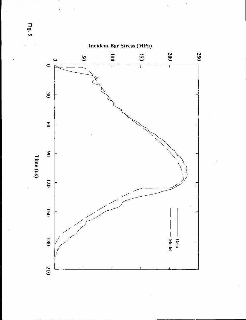
Figures 5 and 6 show data and model predictions for incident stresses from pulse shaped

experiments with hard (HRB 45) and annealed C 11000 pulse shapers, respectively: The pulse

shapers had original thicknesses and diameters of 1.6 mm and 4.8 mm, respectively. The 12.7-

mm-diameter striker and incident bars shown in Fig. 2a had lengths of 152 and 2130 mm,

respectively. The bars were made from high strength maraging VM350 steel (Vasco Pacific,

Montebello, CA) and have density p = 8100 kg/m3, Young’s modulus E = 200 GPa, and bar

wave velocity c = 4970 m/s. The strain gages shown in Fig. 2a are located at 1060 mm from the

impact surface on the incident bar.

The striker bar is launched by a gas gun that has a bore diameter larger than the striker

bar diameter, so the striker bar is fitted with two nylon bore-riders (sabots). The bore-riders are

24

nylon cylinders that make a snug fit for the striker bar in the gun bore and provide a good

alignment for projectile launch. We learned early in this study that the added mass of the bore-

riders needed to be included in the striker bar wave analysis for predicting incident strain pulses.

This added mass is included in the derivation of the elementary theory for the striker bar by

using an effective density p~t,where p~tis the total mass of the striker

by the volume of the striker bar. The wave velocity for the striker,

where E is Young’s Modulus for the striker bar. Model predictions

are in good agreement

We previously

with this approximation.

bar and bore-riders divided

bar is taken as c,t2 = E/p,t,

and measured strain pulses

defined ~ with eq (21 b) as the time for two wave transit times in a striker

bar of length L. For the data and model predictions shown in Figs. 5 and 6, the experiments were

conducted with p~t = 8,750 kg/m3, c~t = 4,780 m/s, L = 152 mm, ~ = 63.6 ~s, and a striking

velocity VO= 17.5 m/s. Both Figs. 5 and 6 show that the onset of unloading is at about t* = 110

ps. So ~s t* <27, and the loading strain in the pulse shaper is calculated from eq (21a) for O< t

<-r and from eq (30) for~ <t <t*. However as with all Hopkinson experimental techniques, we

do not measure stresses or strains in the pulse shaper but infer these quantities through a wave

analysis and downstream strain measurements on the incident bar. Thus, the model that predicts

incident bar stresses shown in Figs. 5 and 6 are calculated from eqs (16), (17a), and

. For t > t* or t greater than about 110 ps, the pulse shaper is unloading.

(39).

We take the

unloading Young’s modulus as EP = 117 GPa in eq (33) and calculate the unloading pulse shaper

strain responses for t* s t < 2-T(2T = 127 ps) from eq (36) and for 2~ < t < 3~ (3T = 191 WS)from

eqs (37a) and (37b). The incident bar stresses predicted for unloading in Figs. 5 and 6 can be

expressed in terms of the strain in the pulse shaper. We combine eqs (13), (14), and (33) and

obtain

25

~i = a“A(I - SP)

o: -. EP(c: – SP) (41)

where UP* and 8P* are the peak pulse shaper stress and strain at the onset of unloading.

A common feature for the hard copper data is a well defined kink found early in the

incident stress-time data. The kink shown in Fig. 5 has an incident stress level of about 70 MPa

and is caused by the transition from elastic to plastic deformation in the pulse shaper. The

incident stress level of this kink can be adjusted by changing the initial pulse shaper diameter. In

addition, the data in Fig. 6 shows the kink is removed for an annealed copper pulse shaper that

has a very small yield strength.

Modified SHPB Experiments with Macor

The analytical models presented in the section, Models for Sample Equilibrium and

Constant Strain Rate, examine the sample response produced by an incident stress. pulse. The

incident stress pulse given by eq (7) is taken as a quadratic function, but these models assume the

sample has a linear stress-strain response. While most brittle materials, such as rocks12 or

ceramics, have quasi-linear, dynamic stress-strain responses, slight deviations from linear can

change the strain-rate histories over the test duration. Because we do not know the sample,

stress-strain response before a test, some experimental trials are required before we achieve

dynamic stress equilibrium and nearly constant strain rate. The analytical models show trends

that help guide and minimize our experimental trials.

26

We begin this process by first conducting a few quasi-static, stress-strain experiments

with a new sample material. Then, we linearize this quasi-static data and obtain a value for Es

for eq (6). Our early SHPB experiments are conducted with nearly linear incident stress pulses

such as those for limestone12 or the incident pulse shown in Fig. 6. We check for sample

equilibrium and nearly constant strain rate with strain measurements and eqs (1a), lb), and (3).

In this study, we learned that it was relatively easy to obtain sample equilibrium and more

difficult to obtain a nearly constant strain rate over most of the test duration. For the Macor

results presented in this section, analytical and experimental trials suggest the concave

downward incident stress pulse shown in Fig. 7 produced a nearly constant strain rate.

To demonstrate our modified SHPB technique, we present results from two pulse shaped

experiments with the machinable glass ceramic, Macor19. Data from experiments with Macor

show that the samples are in dynamic stress equilibrium and have nearly constant strain rates

over most of the duration of the tests. In addition, we carefully bracket sample failure with one

test where the sample fails with catastrophic damage and a second test where the sample is

recovered intact. Thus, intact samples that experience strains beyond the elastic region and post-

peak stresses can be retrieved for microstructural evaluations.

The striker, incident, and transmission bars shown in Fig. 1 were made from high

strength, maraging VM 350 steel (Vasco Pacific, Montebello, CA) and have density p = 8100/

kg/m3, Young’s modulus E = 200 GPa, and bar wave velocity c = 4970 m/s. The incident and

transmission bars had diameters of 19.05 mm and lengths of 2130 and 915 mm, respectively.

27

Strain gages shown in Fig. 1 were located at 1065 mm from the impact surface of the incident

bar and at 458 mm from the sample/ bar interface on the transmission bar. The Macor samples

had a length and diameter of 9.53 mm. To obtain incident stress pulses that would strain the

Macor samples at a nearly constant strain rate over most of the test durations, 10.21-mm-

diameter, 0.79-mm-thick, annealed C 11000 copper pulse shapers were used. All of the above

mentioned parameters remained fixed for the two experiments presented in this section.

However, the first experiment used a 19.05-mm-diameter, 127-mm-long, striker bar, and the

second experiment used a 19.05-mm-diameter, 101.6-mm-long, striker bar. The effective

densities and wave velocities that correct for the added mass of the sabots were p,t = 8790 kg/m3,

c~t= 4770 rds and p~t = 8760 kg/m3, c~t= 4780 rds for the 125-mm-long and 101.6-mm-long

striker bars, respectively. Both striker bars were launched to a striking velocity of 12.2 m/s.

Figures 7, 8, and 9 show data for the experiment conducted with the 127-mm-long

striker bar. In Fig. 7, we show the measured incident stress pulse and a prediction from our pulse

shaping model. Figure 8 shows stresses and stations 1 and 2 shown in Fig. 1. The stress at the

incident bar/ sample interface 01 is calculated from eq (1a) and strains measured on the incident

bar, and stress at the

measured transmitted

transmission bar/ sample interface U2 is calculated from eq (1b) and the

strain. These interface stresses are in reasonably good agreement, which

implies that the sample is nearly in dynamic stress equilibrium. Strain rate in the sample, shown

in Fig. 9, is calculated from eq (3) and the measured reflected strain in the incident bar. The

average strain rate is about 300 s-l over 20 ps to 60 ~s. At about 60 ps the sample begins to fail

and eventually fails with catastrophic damage.

Figures 10, 11, and 12 show data for the experiment conducted with the 101.6-mm-long

striker bar. Figure 12 shows an average strain rate of 280 S-l over 20 ~s to 50 p.s. At 50 ps, the

sample unloads and was recovered intact.

Figure 13 shows dynamic and quasi-static stress-strain data for the Macor samples. The

sample with an average strain rate of ;, = 280 S-*experienced strain beyond the elastic region

28

. ..

and post-peak stress. Samples such as these can be retrieved for post-test, microstructural

evaluations.

Summary

We present analytical models and experimental techniques that provide procedures to

obtain dynamic, compressive stress-strain data for brittle materials. The conventional split

Hopkinson pressure bar apparatus is modified by shaping the incident pulse such that the

samples are in dynamic stress equilibrium and have nearly constant strain rate over most of the

test duration. A thin disk of annealed or hard C 11000 copper is placed on the impact surface of

the incident bar in order to shape the incident pulse. After impact by the striker bar, the copper

disk deforms plastically and spreads the pulse in the incident bar. We present an analytical

model and data that show a wide variety of incident strain pulses can be produced by varying the

geometry of the copper

predictions are in good

disks and the length and striking

agreement with measurements.

velocity of the striker bar. Model

In addition, we present data for a

machinable glass ceramic material, Macor, that shows pulse shaping is required to obtain

dynamic stress equilibrium and nearly constant strain rate over most of the test duration.

Acknowledgments

This work was sponsored by the U.S. Army Engineer Research and Development Center(ERDC) at the Waterways Experiment Station under a laboratory director’s discretionaryresearch program, the U.S. Army Corps of Engineers Hardened Structures Research Programs,and by the Sandia National Laboratories Joint DoD/ DOE Penetration Technology Program.Sandia is a multi-program laboratory operated by Sandia Corporation, a Lockheed MartinCompany, for the United States Department of Energy under Contract DE-AC04-94AL8500.The authors gratefi-dly acknowledge permission from the Director, Geotechnical and StructuresLaboratory, ERDC to publish.this work.

29

References

1. Kolsky, H., “An Investigation of the Mechanical Properties of Materials at Very High Rates

of Loading, “ Proc. Royal SOc. Len., B, 62, 676-700, (1949).

2. Kolsky, H., Stress Waves in Solids. Dover, New York (1963).

3. Nicholas, T., “ Material Behavior at High Strain Rates, “ImPactDynamics, Chapter 8, John

Wiley &Sons, New York, (1982).

4. Nemat-Nasser, S., Isaacs, J. B. and Starrett, J E,, “Hopkinson Techniques for Dynamic

Recovery Experiments, “ Proc. R. Sot. Lend., A, 435, 371-391,(1991).

5. Ramesh, K. T. and Narasimhan, S., “Finite Deformations and the Dynamic Measurement of

Radial Strains in Compression Kolsky Bar Experiments, “ Int. J. Solids Structures 33,

3723-3738, (1996).

6. Gray, G. T., “Classic Split-Hopkinson Pressure Bar Technique, ” LA- UR-99-2347, Los

Alamos National Laboratory, Los Alamos, NM 87545. (1999). To be published in ASA4

Volume 8, Chapter 6A- Mechanical Testing, ASMInternational, Materials Park, OH,

44073.

7. Gray, G. T. and Blumenthal, W. R., “Split-Hopkinson Pressure Bar Testing of Soft

Materials, “ LA- UR-99-4878, Los Alamos National Laboratory, Los Alamos, NM 87545.

(1999). To be published in ASM Volume 8, Chapter 6E- Mechanical Testing, ASM

International, Materials Park, OH, 44073.

8. Yadav, S., Chichili, D. R., and Ramesh, K. T, “The Mechanical Response of a 6061-T6

A1/A1203 Metal Matrix Composite at High Rates of Deformation, ”Acts metall. Mater.

43, 4453-4464, (1995).

9. Rogers, W. P. and Nemat-Nasser, S., “Transformation Plasticity at High Strain Rate in

Magnesia-Partially-Stab ilized Zirconia, “J. Am. Ceram. Sot. 73, 136-139, (1990).

10. Chen, W. and Ravichandran, G., “Dynamic Compressive Failure of a Glass Ceramic Under

Lateral Confinement, ” J Mech. Phys, Solids. 45, 1303-1328, (1997).

30

11. Ravichandran, G. and Subhash, G., “Critical Appraisal of Limiting Strain Rates for

Compression Testing of Ceramics in a Split Hopkinson Pressure Bar, ” J Am. Ceram.

Sot. 77263-267, (1994).

12. Frew, D. J, Forrestal, M. J, and Chen, W., “A Split Hopkinson Bar Technique to Determine

Compressive Stress-Strain Data for Rock Materials, ” EXPERIMENTAL MECHANICS

in press.

13. Duffi, J, Campbell, J. D., and Hawley, R. H., “On the use of a torsional split Hopkinson bar.,

to study rate effects in 1100-0 aluminum, ” ASME J Appl. Mech. 3Z 83-91, (1971).

14. Wu, X J and Gorham, D. A., ‘(Stress Equilibrium in the Split Hopkinson Pressure Bar

Test, ” J PHYS. IV FRANCE 7 C3, 91-96, (1997)

15. Togami, T. C., Baker, W. E. and Forrestal, M J, “A Split Hopkinson Bar Technique to

Evaluate the Performance ofAccelerometers, “ J Appl. Mech. 63, 353-356, (1996).

16. Chen, W., Zhang, B., and Forrestal, M. J,, “A Split Hopkinson Bar technique for low-

impedance materials, “ EXPERIMENTAL MECHANICS 39, 81-85, (1999).

17. Christensen, R. J., Swanson, S. R., and Brown, W. S., “Split-Hopkinson-bar Tests on Rock

under Confining Pressure, “ EXPERIMENTAL MECHANICS 29, 508-513, (1972).

18. Lewis, C. F., “Properties and Selection: Nonferrous Alloys and Pure Metals, ” In Metals

Handbook, 9thEdition, 2, American Society for Metals, Metals Park OH, (1979).

19. Corning Incorporated “Macor A4achineable Glass Ceramic: Safety and Health Issues, “

Technical Bulletin, Macor-03, Corning, New York (1992).

20. Frew, D. J., ‘(The dynamic response of brittle materialsfiom penetration and split

Hopkinson pressure bar experiments, “ Ph. D. thesis, Arizona State University (2000).

21. Davies, E. D. H. and Hunter S. C. ‘(The dynamic compression testing of solids by the method

of the split Hopkinson pressure bar, ” J Mech. Phys. Solids 11, 155-179, (1963).

31

,

22. Baron, H. G. “Stress/strain curves for some metals and alloys at low temperatures and high

rates of strain,” J. Iron St. Inst. 182, 354-365, (1956).

32

Figure Titles

Fig. 1- Schematic of a conventional split Hopkinson pressure bar (SHPB) or Kolsky bar

Fig. 2- Schematic of the loading end of a SHPB with a pulse shaper

Fig. 3- Data and response fimction for hard (HRB 45) Cl 1000 copper

Fig. 4- Data and response functions for annealedC11000 copper

Fig. 5- Incident bar stress data and model prediction for a hard (HRB 45) C 11000 copper pulse

shaper

Fig. 6- Incident bar stress data and model prediction for an annealed Cl 1000 copper pulse shaper

Fig. 7- Incident bar stress data and model prediction for an annealed C 11000 copper pulse shaper

Fig. 8- Interface stresses from a pulse shaped SHPB experiment with a Macor sample

Fig. 9- Strain rate from a pulse shaped SHPB experiment with a Macor sample

Fig. 10- Incident bar stress data and model prediction for an annealedC11000 copper pulse

shaper

Fig. 11-Interface stresses from a pulse shaped SHPB experiment with a Macor sample

Fig. 12-Strain rate from a pulse shaped SHPB experiment with a Macor sample

Fig. 13-Quasi-static and dynamic stress-strain data for Macor

33

t(’v % “d)

L

(c)

(“q ‘“P)~ad~qs aslnd

.

/

J‘A

TG“.C.J

True Axial Stress (MPa)+ # +

s s a Oc o No 0

a

o 00 0

0 00

0 G a o

I I I I I I I— .— —-”

———

——

❑

k•1•1

\■ o

LJ..

o

‘h o

o

0

0

oid

ou

o

4

True Axial Stress (MPa)

mo0

— I I I I I I 1 1 I

\\\l

N!!\CAh+ ‘Lm● 9’, 0

\o

&\

\

\

● 0) \\

I

I

I ❑ moeI

I

000

\ \

m

Incident Bar Stress (MPa)

ha

o a o G ~o

%o 0 0

0

ho

cco

N

o

\

_—

/

/

/

/

/

/

/

.

-nG.

Incident Bar Stress (MPa)

o

wo

0

0

mo

Incident Bar Stress (MPa)

—_

/

/

/

/

/

o

0

Stress (MPa)

Ao0

ao0

\

\ I.

I\ I

I

I1“

11

\

\

\,

/-/-

/-/

-nG“.

o

0

0

Strain Rate (s -1)

N’o

Ao

00

nG’,

Incident Bar Stress (Ml?a)+ -

m o0 0

#o

%o

zG o

I I I I

/

}

o

ao

(no

o

Stress (MPa)

u & mo 00 z o

ao0

400

\‘.

W3o

wo0

-nz’.

o

WIo

c!o

0

Stress (MPa)

-g

o

o

00

Stress (MPa)

. I 1 I I 1 t

“CM \“Oo+>

,! \

I I

\