JHEP11(2018)110

Published for SISSA by Springer

Received: October 13, 2018

Accepted: November 8, 2018

Published: November 19, 2018

De Sitter vacua in no-scale supergravity

John Ellis,a,b,c Balakrishnan Nagaraj,d Dimitri V. Nanopoulosd,e,f and Keith A. Oliveg

aTheoretical Particle Physics and Cosmology Group, Department of Physics,

King’s College London, London WC2R 2LS, U.K.bTheoretical Physics Department, CERN,

CH-1211 Geneva 23, SwitzerlandcNational Institute of Chemical Physics & Biophysics,

Ravala 10, 10143 Tallinn, EstoniadGeorge P. and Cynthia W. Mitchell Institute for Fundamental Physics and Astronomy,

Texas A&M University, College Station, TX 77843, U.S.A.eAstroparticle Physics Group, Houston Advanced Research Center (HARC),

Mitchell Campus, Woodlands, TX 77381, U.S.A.fAcademy of Athens, Division of Natural Sciences,

Athens 10679, GreecegWilliam I. Fine Theoretical Physics Institute, School of Physics and Astronomy,

University of Minnesota, Minneapolis, MN 55455, U.S.A.

E-mail: John.Ellis@cern.ch, nbala@physics.tamu.edu,

dimitri@physics.tamu.edu, olive@umn.edu

Abstract: No-scale supergravity is the appropriate general framework for low-energy

effective field theories derived from string theory. The simplest no-scale Kahler potential

with a single chiral field corresponds to a compactification to flat Minkowski space with a

single volume modulus, but generalizations to single-field no-scale models with de Sitter

vacua are also known. In this paper we generalize these de Sitter constructions to two-

and multi-field models of the types occurring in string compactifications with more than

one relevant modulus. We discuss the conditions for stability of the de Sitter solutions and

holomorphy of the superpotential, and give examples whose superpotential contains only

integer powers of the chiral fields.

Keywords: Supergravity Models, Superstring Vacua

ArXiv ePrint: 1809.10114

Open Access, c© The Authors.

Article funded by SCOAP3.https://doi.org/10.1007/JHEP11(2018)110

JHEP11(2018)110

Contents

1 Introduction 1

2 Single-field models 2

2.1 No-scale supergravity models 2

2.2 Minkowski solutions 4

2.3 De Sitter solutions 5

3 Two-field models 6

3.1 Minkowski solutions 6

3.2 De Sitter solutions 10

3.3 Stability analysis 11

4 N-field models 13

4.1 Minkowski Solutions 13

4.2 De Sitter solutions 15

4.3 Stability analysis 16

5 Conclusion and outlook 18

1 Introduction

If one assumes that N = 1 supersymmetry holds down to energies hierarchically smaller

than the Planck mass, low-energy dynamics must be governed by some N = 1 supergravity.

It is known that the energy density in the present vacuum is very small compared, e.g., to

typical energy scales in the Standard Model. It was therefore natural to look for N = 1

supergravity theories that yielded a vanishing cosmological constant without unnatural fine

tuning, and a total scalar potential that is positive definite. The unique Kahler potential

for such an N = 1 supergravity model with a single chiral superfield φ (up to canonical

field redefinitions) was found in [1] to be

K = − 3 ln(φ+ φ†

). (1.1)

In [2] this was dubbed ‘no-scale supergravity’, because the scale of supersymmetry breaking

is undetermined at the tree level, and it was suggested that the scale might be set by

perturbative corrections to the effective low-energy field theory. The single-field model (1.1)

was explored in more detail in [3] (EKN), and the generalization to more superfields was

developed in [4].1 It was shown subsequently that no-scale supergravity emerges as the

1For a review of early work on no-scale supergravity, see [5].

– 1 –

JHEP11(2018)110

effective field theory resulting from a supersymmetry-preserving compactification of ten-

dimensional supergravity, used as a proxy for compactification of heterotic string theory [6].

In recent years interest has grown in the possibility of string solutions in de Sitter

space, for at least a couple of practical reasons. One is the discovery that the expansion of

the Universe is accelerating due to non-vanishing vacuum energy that is small relative to

the energy scale of the Standard Model [7, 8] (for the most recent observational constraints

see [9]). The other is the growing observational support for inflationary cosmology [10–16],

according to which the Universe underwent an early epoch of near-exponential quasi-de

Sitter expansion driven by vacuum energy that was large compared with the energy scale

of the Standard Model, but still hierarchically smaller than the Planck scale. At the time

of writing there is an ongoing controversy whether string theory in fact admits consistent

solutions in de Sitter space [17–29].

If string theory does indeed admit de Sitter solutions and approximate supersymmetry

with scales hierarchically smaller than the string scale, their low-energy dynamics should be

described by some suitable supergravity theory that is capable of incorporating the breaking

of supersymmetry that is intrinsic in de Sitter space. Since string compactifications yield

no-scale supergravity as an effective low-energy field theory, it is natural to investigate

how de Sitter space could be accommodated within no-scale supergravity.2 This question

was studied already in [3], and the purpose of this paper is to analyze this question in

more detail and generality, extending the previous single-field analysis of [3, 36] to no-scale

models with multiple superfields that are characteristic of generic string compactifications.

These models may provide a useful guide to the possible forms of effective field theories

describing the low-energy dynamics in de Sitter solutions of string theory, assuming that

they exist.

The outline of this paper is as follows. In section 2 we review the original motivation

and construction of no-scale supergravity with a vanishing cosmological constant [1], and

also review the construction in [3, 36] of no-scale supergravity models with non-vanishing

vacuum energy. Section 3 describes the extensions of these models to no-scale supergravity

models with two chiral fields, which have an interesting geometrical visualization. The de

Sitter construction is extended to multiple chiral fields in section 4. In each case, we discuss

the requirements of stability of the vacuum and holomorphy of the superpotential, and give

examples of models whose superpotentials contain only integer powers of the chiral fields.

Finally, section 5 summarizes our conclusions and presents some thoughts for future work.

2 Single-field models

2.1 No-scale supergravity models

We recall that the geometry of a N = 1 supergravity model is characterized by a Kahler

potential K that is a Hermitian function of the complex chiral fields φi. The kinetic terms

of these fields are

Kji

∂φi∂xµ

∂φ†j∂xµ

where Kji ≡

∂2K

∂φi∂φ†j(2.1)

2For other approaches, see [30–35].

– 2 –

JHEP11(2018)110

is the Kahler metric. Defining also Ki ≡ ∂K/∂φi and analogously its complex conjugate

Ki, the tree-level effective potential is

V = eK[KjK−1ji Ki − 3

]+

1

2DaDa , (2.2)

where K−1ji is the inverse of the Kahler metric (2.1) and 12D

aDa is the D-term contribution,

which is absent for chiral fields that are gauge singlets as we assume here.

In this section we consider the case of a single chiral field φ, in which case it is easy to

verify that the first term in (2.2) can be written in the form

V (φ) = 9 e4K/3 K−1φφ†

∂φ∂φ†e−K/3 . (2.3)

It is then clear that the unique form of K with a Minkowski solution, for which V = 0, is

K = − 3 ln(f(φ) + f †(φ†)

), (2.4)

where f is an arbitrary analytic function. In fact, since physical results are unchanged

by canonical field transformations, one can transform f(φ) → φ and recover the simple

form (1.1) of the Kahler potential for a no-scale supergravity model with a single chiral field.

We note that this Kahler potential describes a maximally-symmetric SU(1,1)/U(1)

manifold whose Kahler curvature Rji ≡ ∂i∂j lnKj

i obeys the simple proportionality

relationRjiKji

≡ R =2

3, (2.5)

which is characteristic of an Einstein-Kahler manifold.

This model was generalized in EKN [3], where general solutions for all flat potentials

were found. The SU(1,1) invariance in eq. (2.4) holds whenever3

R ≡RjiKji

=2

3α, (2.6)

which corresponds (up to irrelevant field redefinitions) to the extended Kahler potential

G = K + lnW (φ) + lnW †(φ†) , (2.7)

where

K = − 3αln(φ+ φ†) , (2.8)

we assume α > 0, and W (φ) is the superpotential.4 In this case the effective potential is

V = eG[GjK−1ji Gi − 3

]. (2.9)

3We note that in extended SU(N,1) no-scale models [4] that include N − 1 matter fields, yi, with the

Kahler potential K = −3α log(φ + φ† − yiy†i /3), the Kahler curvature becomes R = (N + 1)/3α. Our

constructions can be generalized to this case, but such generalizations lie beyond the scope of this paper.4Starobinsky-like models with α 6= 1 were discussed in [37]. Such models were later dubbed α-attractors

in [36, 38, 39].

– 3 –

JHEP11(2018)110

EKN found 3 classes of solutions with a constant scalar potential [3], namely

1) W = a and α = 1 , (2.10)

2) W = aφ3α/2 , (2.11)

3) W = aφ3α/2(φ3√α/2 − φ−3

√α/2) . (2.12)

Solution 1) corresponds to the V = 0 Minkowski solution discussed above, whereas solutions

2) and 3) yield potentials that are constant in the real direction, but are in unstable in the

imaginary direction. As we discuss further below, stabilization in the imaginary direction

is straightforward and allows these solutions to be used for realistic models with constant

non-zero potentials in the real direction. We find that 2) leads to anti-de Sitter solutions

with V = −3/8α · a2 and 3) leads to de Sitter solutions5 with V = 3 · 22−3α · a2. We

note that in the particular case α = 1 this reduces to W = a (φ3 − 1), which yields the de

Sitter solution discussed in [36]. This was utilized in [40] when making the correspondence

between no-scale supergravity and R2 gravity.

In the following subsections, we first generalize the Minkowski solution (2.10), and then

show that de Sitter solutions can be obtained as combinations of Minkowski solutions.

These aspects of the solutions will subsequently be used to generalize them to model

theories with multiple moduli.

2.2 Minkowski solutions

We consider the N = 1 no-scale supergravity model with a single complex chiral field φ

described by the Kahler potential given in (2.8) and the superpotential W (φ) is a monomial

of the form

W = aφn , (2.13)

and we seek the value of n that admits a Minkowski solution with V = 0. Defining

φ ≡ x+ iy, the potential along real field direction x is given by

V = 2−3α ·(

(2n− 3α)2

3α− 3

)· a2 · x2n−3α . (2.14)

We can obtain a Minkowski solution by setting to zero the term in the brackets:

(2n− 3α)2

3α= 3. (2.15)

Solving the above equation for n, we find two solutions [36]:

n± =3

2(α±

√α) . (2.16)

We note that n− = 0 for α = 1, corresponding to the EKN solution (2.10) listed above.

However, we see that in addition to this n = 0 solution, n = 3 also yields a Minkowski

solution with V = 0 in all directions in field space.

5We correct here a typo in the third solution given in [3].

– 4 –

JHEP11(2018)110

Although such solutions exist for any α, for the superpotential to be holomorphic we

need n− ≥ 0, which requires α ≥ 1. Clearly, integer solutions for n are obtained whenever

α is a perfect square [36].

It is possible to go from one superpotential to another via a Kahler transformation:

K −→ K + λ(φ) + λ†(φ†), W −→ e−λ(φ)W . (2.17)

with λ(φ) = ±3√α lnφ. In general, the solutions (2.16) can be thought of as corresponding

to endpoints of a line segment of length 3√α centred at 3α/2. Though this appears trivial,

extensions of this geometric visualization will be useful in the generalizations to multiple

fields discussed below.

For α 6= 1, the two solutions yield V = 0 only along the real direction, and the mass

squared of the imaginary component y along the real field direction for x > 0 and y = 0 is

given by

m2y = 22−3α · (α− 1)

α· a2 · x±3

√α, (2.18)

where the ± in the exponent corresponds to the two solutions n±. From this it is clear

that the Minkowski solutions are stable for α ≥ 1.

There are two aspects of the single-field model that we emphasize here, because they

generalize in an interesting way to multi-field models. The first is the fact that there are

two solutions for n and the second is that, when α = 1, we get a Minkowski solution with

a potential that vanishes everywhere.

2.3 De Sitter solutions

As was shown in EKN, de Sitter solutions can be found with the Kahler potential (2.8)

and a superpotential of the form (2.12), which may be written as

W = a (φn− − φn+) , (2.19)

where n± are given in (2.16). In this case the potential along the real field direction y = 0 is

V = 3 · 22−3α · a2 . (2.20)

Thus, the de Sitter solution is obtained by taking the difference of the two “endpoint”

solutions mentioned above.

Unfortunately, this de Sitter solution is not stable for finite α. However, this can be

remedied by deforming the Kahler potential to the following form [37, 41]:

K = − 3α ln(φ+ φ† + b(φ− φ†)4) : b > 0 . (2.21)

The addition of the quartic stabilization term does not modify the potential in the real

direction, which is still given by (2.20). However, the squared mass of the imaginary

component y is now given by

m2y =

22−3α

α· a2 · x−3

√α ·(α(x3

√α − 1)2 − (1− 96bx3)(x3

√α + 1)2

). (2.22)

The stability requirement m2y ≥ 0 is achieved when α ≥ 1. In figure 1 we plot the stabilized

potential for a = b = α = 1, and we see that the potential is completely flat along the line

y = 0 and is stable for all values of x > 0.

– 5 –

JHEP11(2018)110

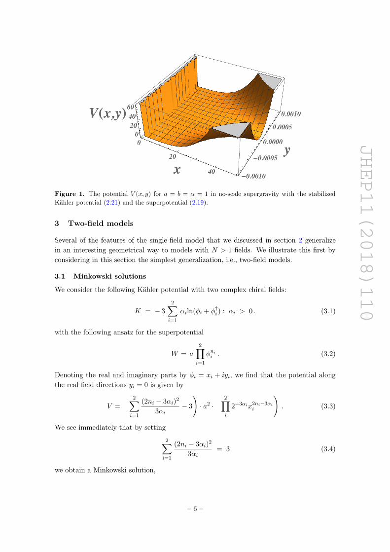
Figure 1. The potential V (x, y) for a = b = α = 1 in no-scale supergravity with the stabilized

Kahler potential (2.21) and the superpotential (2.19).

3 Two-field models

Several of the features of the single-field model that we discussed in section 2 generalize

in an interesting geometrical way to models with N > 1 fields. We illustrate this first by

considering in this section the simplest generalization, i.e., two-field models.

3.1 Minkowski solutions

We consider the following Kahler potential with two complex chiral fields:

K = − 32∑i=1

αiln(φi + φ†i ) : αi > 0 . (3.1)

with the following ansatz for the superpotential

W = a2∏i=1

φnii . (3.2)

Denoting the real and imaginary parts by φi = xi + iyi, we find that the potential along

the real field directions yi = 0 is given by

V =

(2∑i=1

(2ni − 3αi)2

3αi− 3

)· a2 ·

(2∏i

2−3αix2ni−3αii

). (3.3)

We see immediately that by setting

2∑i=1

(2ni − 3αi)2

3αi= 3 (3.4)

we obtain a Minkowski solution,

– 6 –

JHEP11(2018)110

We observe that (3.4) describes an ellipse in the (n1, n2) plane centred at

(3α1/2, 3α2/2). All choices of (n1, n2) lying on this ellipse yield a Minkowski solution.

In this way, the line segment centred at 3α/2 in the single-field model that yielded

Minkowski endpoints is generalized, and we obtain a one-dimensional continuum subspace

of Minkowski solutions. We can conveniently parametrize the solutions for ni in (3.4) as

the points on the ellipse corresponding to unit vectors ~r = (r1, r2) with r21 + r22 = 1:

ni± =3

2

αi ± ri√∑2j=1

r2jαj

, i = 1, 2 . (3.5)

The unit vector ~r should be located starting at the centre of the ellipse, and defines a

direction on its circumference. The operation ~r → −~r in equation (3.5) takes a point

on the ellipse to its antipodal point, an observation we use later to construct de Sitter

solutions. We note also that holomorphy requires both n1, n2 ≥ 0, i.e.

αi +ri√∑2j=1

r2jαj

≥ 0 , i = 1, 2 . (3.6)

As in the case of the single-field model, we can move from one point on the ellipse to

another point via a Kahler transformation. This is possible because the superpotential is

just a monomial.

Integer solutions for the values of ni are also possible in the two-field case. The full set

of solutions in the single-field case are valid for n1± when n2+ = n2− (and similarly when

1↔ 2). More generally, solutions can be found by writing

(n1+ − n1−)2 = λ1(n1+ + n1−) and (n2+ − n2−)2 = λ2(n2+ + n2−) , (3.7)

with λi is non-negative and λ1 + λ2 = 3. As one example out of an infinite number of

solutions, choosing λ1 = 1 and λ2 = 2 gives (n1+, n1−) = (3, 1) and (n2+, n2−) = (6, 2).

In general, points around the ellipse yield potentials that are flat only in the real

direction and, as in the single-field model, may not be stable in the imaginary directions.

The masses of the imaginary component fields y1, y2 are given by

m2yi =

22−3(α1+α2)

α2i

·

α2i −

r2i(∑2j=1

r2jαj

) · a2 · x2n1−3α1

1 x2n2−3α22 , i = 1, 2 . (3.8)

The stability requirement m2yi ≥ 0 for xi > 0 implies

α2i −

r2i(∑2j=1

r2jαj

) ≥ 0 , i = 1, 2 . (3.9)

It is easy to see that if the stability conditions are satisfied then the holomorphy condi-

tions (3.6) are satisfied. Since the left hand side of (3.9) is proportional to ni+ni−, points

– 7 –

JHEP11(2018)110

0.0 0.5 1.0 1.5 2.0 2.5 3.0

0.0

0.5

1.0

1.5

2.0

2.5

3.0

α1

α2

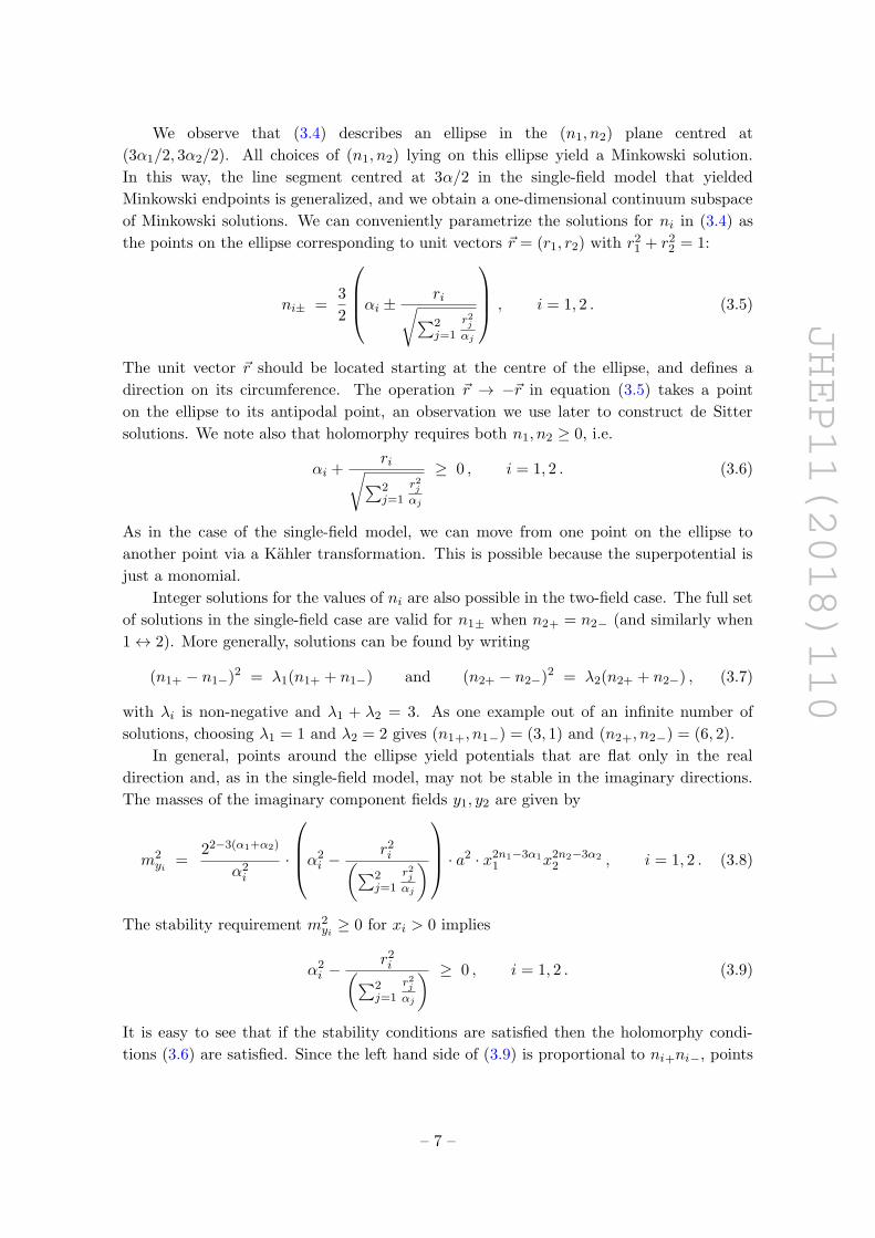
Figure 2. The shaded regions are the allowed values of α1, α2 for the illustrative choices ~r =

(1/√

2, 1/√

2) (green) and ~r = (1/√

10, 3/√

10) (blue). There are kinks located at (α1, α2) =

(1/2, 1/2) and (α1, α2) = (1/4, 3/4) for the two choices of unit vectors. The black line is α1+α2 = 1.

on the ellipse that give stable Minkowski solution are those that are holomorphic so long

as their antipodal points are also holomorphic.

However, given a choice of unit vector, ~r, this condition is not satisfied for all choices

of αi. We show in figure 2 the allowed domain in the (α1, α2) plane for which the stability

conditions (3.9) (and hence also the holomorphy conditions (3.6)) are satisfied, for two

illustrative choices of the unit vector ~r. The allowed region for ~r = (1/√

2, 1/√

2) is shaded

green and behind it (shaded blue) is the allowed region when ~r = (1/√

10, 3/√

10). For

both choices of ~r, there is a kink in the allowed domain where it meets the line given by

α1 + α2 = 1. At the kink, for all choices of ~r, the potential is completely flat and vanishes

in all directions in field space. The position of the kink can be calculated by solving the

stability condition along this line:

α1 =r21 −

√r21 − r41

2r21 − 1. (3.10)

For the two examples shown in figure 2, r1 = 1/√

2 implies α1 = 1/2 at the kink, and

r1 = 1/√

10 implies α1 = 1/4. In fact, because of the sign ambiguity, there are four unit

vectors for each solution, corresponding to the ambiguous signs of r1 and r2.

Another projection of the domain of stability is shown in figure 3, which displays the

allowed regions in the (α1, r21) plane for the fixed values α2/α1 = 1, 2, 3, 5, 10, as illustrated

by the curves, respectively. Each pair of curves (red, green, purple, blue and black for

increasing α2/α1) corresponds to the two equalities in (3.9), and the positivity inequalities

are satisfied to the right of each pair of lines for a given value of α2/α1. For example, when

α2/α1 = 1 (shown by the solid red curves), all values of r21 are allowed if α1 ≥ 1, while no

values are allowed when α1 < 1/2. The point where the curves meet corresponds to the

– 8 –

JHEP11(2018)110

r12

α1

0.0 0.5 1.0 1.5 2.00.0

0.2

0.4

0.6

0.8

1.0

α2/α

1 = 1, 2, 3, 5, 10

Figure 3. The allowed values of α1, r21 for fixed ratios of α2/α1 = 1, 2, 3, 5, 10. The two sets of

curves are derived from the two constraint equations in (3.9). The stability inequality is satisfied for

points with α1 to the right of both curves of the same colour (red, green, purple, blue and black for

increasing α2/α1). The point at which the two curves meet corresponds to the kink that appears

in figure 2 when α1 + α2 = 1.

kink when α1 = α2 = 1/2 and r21 = 1/2 that was seen in figure 2 where the green shaded

region touches the black line. When α2/α1 = 3 (shown by medium dashed purple curves),

the kink occurs when these two curves meet at α1 = 1/4 and r21 = 1/10.

The lower ellipse (3.4) in the (n1, n2) plane shown in figure 4 corresponds to this second

example. As this corresponds to the position of the kink, only a single value of r21 = 1/10

is allowed. The four red spots in the figure correspond to the four different vectors ~r =

(±1/√

10,±3/√

10). These four unit vectors correspond to four different superpotentials via

the relation (3.5), which give (n1, n2) = (3/4, 9/4), (3/4, 0), (0, 9/4), (0, 0). When (α1, α2) =

(1/4, 3/4), each of the four superpotentials defined by the pair ni yields a true Minkowski

solution. However, because we are at the kink, there are no other stable solutions.

Choosing a larger value of α1 while keeping α2/α1 fixed would increase the allowed

range in r21 (as seen in figure 3) and would allow a continuum of stable Minkowski solutions

along the real direction in field space. This is seen in the upper ellipse in figure 4, where

we have chosen α1 = 1/2 and α2 = 3/2. In this case, the stability constraint, which can

be read off figure 3 for α2/α1 = 3 at the chosen value of α1, yields r1 < 1/2. Unit vectors

with r1 < 1/2 correspond to arcs along the upper ellipse in figure 4. These are further

shortened by the holomorphy requirement that ni ≥ 0, and the resulting allowed solutions

are shown by the red arc segments in the upper ellipse.

To summarize this discussion of Minkowski solutions in the two-field case:

1) For any generic unit vector ~r, there is always a kink in the boundary of the allowed

values of (α1, α2) as shown in figure 2, and these kink solutions always satisfy α1 +

α2 = 1 with α1 given by (3.10). The kink solutions give a vanishing potential V = 0

in all directions in field space.

2) For any pair (α1, α2) satisfying α1 + α2 = 1, there are four unit vectors that are

– 9 –

JHEP11(2018)110

-1.0 -0.5 0.0 0.5 1.0 1.5 2.0 2.5

0

1

2

3

4

n1

n2

Figure 4. Minkowski solutions for α1 = 1/4, α2 = 3/4 (lower ellipse) and α1 = 1/2, α2 = 3/2

(upper ellipse). In the former case only the four red points corresponding to ~r = (±1/√

10,±3/√

10)

are allowed, whereas in the latter case the red arc segments correspond to allowed solutions.

determined by inverting (3.10), namely

r1 = ± α1√1− 2α1 + 2α2

1

. (3.11)

The four values of the ni that correspond to these choices are (n1, n2) =

(0, 0), (3α1, 0), (0, 3α2), (3α1, 3α2).

3) For α1 + α2 > 1, a continuum of stable Minkowski solutions exist and, when α1 ≥ 1

with α2/α1 ≥ 1, the entire ellipse (that is, all unit vectors ~r) yield stable Minkowski

solutions in the real directions of field space.

4) The holomorphy conditions (3.6) are satisfied automatically if the stability condi-

tions (3.9) are satisfied.

5) There is an infinite set of Minkowski solutions with positive integer powers of the

fields in the superpotential.

3.2 De Sitter solutions

We recall that in the single-field model we were able to construct a de Sitter solution

by combining the two superpotentials corresponding to Minkowski solutions that can be

visualized as opposite ends of a line segment. In the two-field model, we have a continuum

of superpotentials that give Minkowski solutions, which are described by an ellipse (3.4). In

this case it is possible to to construct new de Sitter solutions by combining superpotentials

– 10 –

JHEP11(2018)110

corresponding to antipodal points on the ellipse (3.4). For example, consider the following

combined superpotential:

W = a(φn1+

1 φn2+

2 − φn1−1 φ

n2−2

). (3.12)

It is easy to see that the scalar potential in the real field direction is a de Sitter solution:

V = 3 · 22−3α1−3α2 · a2 (3.13)

in this case.

For the example described by the lower ellipse in figure 4, one example of a de Sit-

ter solution is found by taking antipodal points corresponding to the red spots. When

~r = (1/√

10, 3/√

10), we have W = a(φ3/41 φ

9/42 − 1), which is the unique solution with a

holomorphic superpotential that results in a flat de Sitter potential in the real direction.

However, as we discuss further below, this solution is actually not stable.

As an alternative example, we consider a two-field model with α1 = 1 and α2 = 2. The

Minkowski solutions in this case are described by the ellipse (3.4) in (n1, n2) space shown in

figure 5, whose centre is at (3/2, 3). In this case, the entire ellipse can be used to construct

de Sitter solutions, as all possible unit vectors ~r are allowed since α1 > 1 (see figure 3).

As in the previous example, we can use antipodal points to construct de Sitter solutions,

as illustrated in figure 5. One such pair of antipodal points is (3, 3), (3, 0), corresponding

to ~r = (1, 0), indicated by the horizontal orange line in figure 5. The corresponding

superpotential is

W = a2(φ31φ

32 − φ32

), (3.14)

so that the fields appear in the superpotential with positive integer powers. This example

yields a de Sitter potential with the potential value

V = 3 · 2−7 · a2. (3.15)

along the real field directions. A continuum of de Sitter solutions for real field values are

possible for different choices of ~r, e.g., the choice indicated in figure 5 by the blue line, all

with the potential given by eq. (3.15).

3.3 Stability analysis

As in the single-field case, the de Sitter solutions of the two-field model require modification

in order to be stable. Stable solutions can easily be found by deforming the Kahler potential

to include stabilizing quartic terms:

K = − 3

2∑i=1

αiln(φi + φ†i + bi(φi − φ†i )4) : bi > 0 . (3.16)

With this modification the potential along real field directions is still given by equa-

tion (3.13). To prove the stability of the two-field de Sitter solution with the quartic mod-

ification of the Kahler potential, we calculate the Hessian matrix ∂2V/∂yi∂yj : i, j = 1, 2

– 11 –

JHEP11(2018)110

- 1 0 1 2 3 4

- 1

0

1

2

3

4

5

6

n1

n2

Figure 5. The Minkowski solutions for α1 = 1 and α2 = 2 are described by an ellipse in (n1, n2)

space. Lines passing through the center of the ellipse connect antipodal points, as illustrated with

two examples.

along the real field directions, and demand that it be positive semi-definite. The Hessian

matrix along the real field directions is of the form

a2(

3.21−3α1−3α2

α2r21 + α1r22

)[ x−21 A1 x−11 x−12 B

x−11 x−12 B x−22 A2

], (3.17)

where

A1 = w−1(α21r

22(1 + 4w + w2) + α1α2r

21(1− w)2 + α2r

21(96b1x

31 − 1)(1 + w)2

), (3.18)

A2 = w−1(α22r

21(1 + 4w + w2) + α1α2r

22(1− w)2 + α1r

22(96b2x

32 − 1)(1 + w)2

), (3.19)

B = −6α1α2r1r2 , (3.20)

we have defined

w ≡ x

3r1√r21α1

+r22α2

1 x

3r2√r21α1

+r22α2

2 , (3.21)

and the Hessian matrix is positive semi-definite if the condition

H ≡ A1A2 ≥ B2 (3.22)

is satisfied.

The stability condition (3.22) for generic α1, α2, b1, b2 and ~r is(α21r

22(1 + 4w + w2) + α1α2r

21(1− w)2 + α2r

21(96b1x

31 − 1)(1 + w)2

)×

α22r

21(1 +4w+w2) + α1α2r

22(1−w)2 + α1r

22

96b2w

1r2

√r21α1

+r22α2

x(3r1/r2)1

− 1

(1 + w)2

− 36α2

1α22r

21r

22w

2 ≥ 0 . (3.23)

– 12 –

JHEP11(2018)110

A general stability analysis is intractable, so we have considered the simplified case: α1 =

α2 ≡ α and ~r = (1/√

2, 1/√

2), for which the positivity condition (3.22) becomes(2α(1 + w + w2) + (96b1x

31 − 1)(1 + w)2

)×(2α(1 + w + w2) + (96b2x

32 − 1)(1 + w)2

)≥ 36α2w2 .

(3.24)

Eliminating x2 in favour of x1 and w via equation (3.21), this inequality becomes(2α(1 + w + w2) + (96b1x

31 − 1)(1 + w)2

)×

(2α(1 + w + w2) +

(96b2

w√

2/α

x31− 1

)(1 + w)2

)− 36α2w2 ≥ 0 .

(3.25)

We note that (96b1x31 − 1) dominates for x1 1 and

(96b2

w√

2/α

x31− 1)

dominates for

x1 1, implying that there is an extremum for some intermediate value of x1. This occurs

at x1 = (b2/b1)1/6w1/(3

√2α), and is a global extremum. Whether it is a maximum or a

minimum depends on the sign of 2α(1 + w + w2)− (1 + w)2, and it is non-negative for

α ≥ 2

3. (3.26)

This is a necessary condition for the inequality (3.25) to be satisfied. We have not explored

the full range of possible values of b1 and b2 when α1 = α2 = α, but have checked that the

stability condition (3.25) is always satisfied if b1 = b2 = 1 and α ≥ 2/3, irrespective of the

value of w. We have also found that when α1 6= α2 the sum α1 + α2 ≥ 4/3.

We have also considered the case ~r = (0, 1) with b1 = b2 = 1. The inequality (3.23)

reduces in this case to

α2(1− w)2 + (1 + w)2(96w1/√α2 − 1) ≥ 0 , (3.27)

which is always satisfied for α2 ≥ 1. It is easy to check that the same is true for the

case ~r = (1, 0). Based on these cases and the previous example with ~r = (1/√

2, 1/√

2),

we expect that there are generic stable solutions for a range of ~r in the first and third

quadrants where r1/r2 > 0. However, the situation is different when r1/r2 < 0. We find

that the inequality (3.22) cannot be satisfied for ~r = (−1/√

2, 1/√

2) and b1 = b2 = 1, so

there are no stable de Sitter solutions, and we expect the same to be the case for other

choices of ~r in the second or fourth quadrant.

In summary, we have established the existence of stable de Sitter solutions only when

~r is in either first or third quadrant.

4 N-field models

Finally, we generalize the above set of examples to models with multiple fields N > 2.

4.1 Minkowski Solutions

The natural generalization of the Kahler potential in (3.1) is simply a sum of N simi-

lar terms:

K = − 3

N∑i=1

αiln(φi + φ†i ) . (4.1)

– 13 –

JHEP11(2018)110

Similarly, we adopt the following ansatz for the superpotential:

W = a

N∏i=1

φnii , (4.2)

in which case the potential along the real field directions xi is

V =

(N∑i=1

(2ni − 3αi)2

3αi− 3

)· a2 ·

(N∏i

2−3αix2ni−3αii

). (4.3)

We can obtain Minkowski solutions along the real field directions by setting

N∑i=1

(2ni − 3αi)2

3αi= 3 , (4.4)

which describes an ellipsoid in (n1, . . . , nN ) space whose centre is at (3α1/2, . . . , 3αN/2).

Once again we find a continuum of Minkowski solutions. The points on the ellipsoid can

be parametrized conveniently using an N -dimensional unit vector ~r:

ni =3

2

αi +ri√∑Nj=1

r2jαj

i = 1, . . . , N ; r21 + . . .+ r2N = 1 , (4.5)

where the unit vector ~r is to be considered as anchored at the centre of the ellipsoid. To

ensure holomorphy of the superpotential we need ni ≥ 0, and the masses of the imaginary

field components yi are given by

m2yi =

22−3(∑αi)

α2i

·

α2i −

r2i(∑Nj=1

r2jαj

) · a2 · N∏

j=1

x2nj−3αjj , i = 1, . . . , N . (4.6)

For stability, we impose conditions similar to (3.9), namely:

α2i −

r2i(∑2j=1

r2jαj

) ≥ 0 i = 1, . . . , N . (4.7)

As in two-field models, ensuring these stability conditions are satisfied implies that the

holomorphy conditions are also satisfied. For a given unit vector ~r, one can ask what values

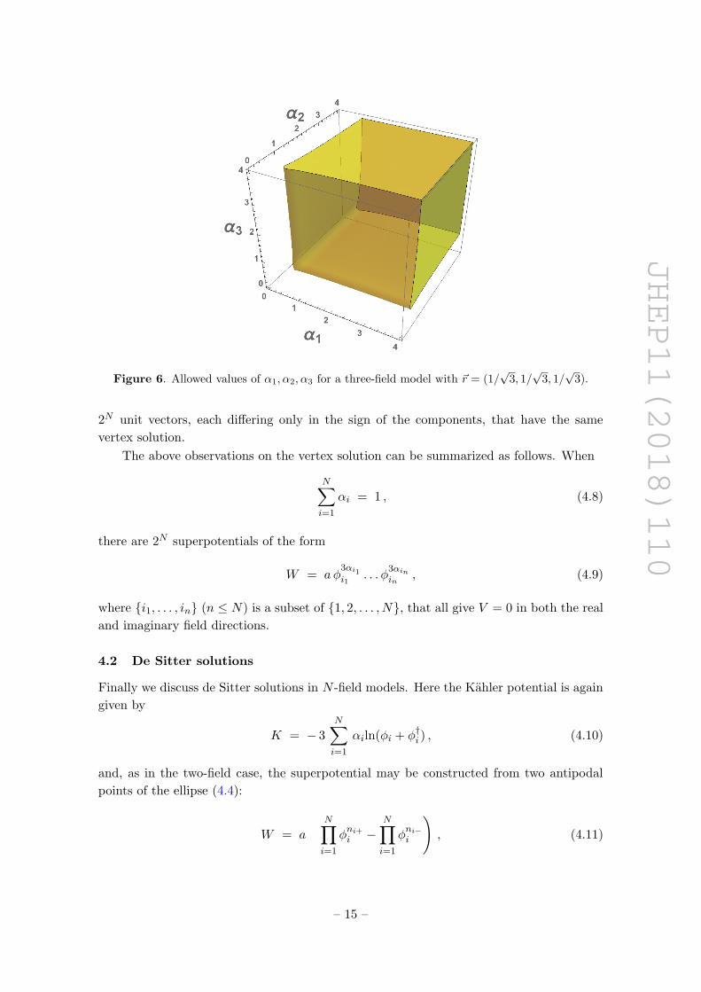
of α1, . . . , αN satisfy the stability conditions. We find a multidimensional region analogous

to that in figure 2, with a vertex that satisfies α1 + . . .+ αN = 1. We show in figure 6 the

allowed region of α1, α2 and α3 for a three-field model with ~r = (1/√

3, 1/√

3, 1/√

3).

The vertex is a special solution that corresponds to V = 0 in both the real and

imaginary field directions. When the sign of one of the components of ~r is changed, the

region in α1, . . . , αN space that satisfies (4.7) remains the same. Therefore, there are

– 14 –

JHEP11(2018)110

Figure 6. Allowed values of α1, α2, α3 for a three-field model with ~r = (1/√

3, 1/√

3, 1/√

3).

2N unit vectors, each differing only in the sign of the components, that have the same

vertex solution.

The above observations on the vertex solution can be summarized as follows. When

N∑i=1

αi = 1 , (4.8)

there are 2N superpotentials of the form

W = aφ3αi1i1

. . . φ3αinin

, (4.9)

where i1, . . . , in (n ≤ N) is a subset of 1, 2, . . . , N, that all give V = 0 in both the real

and imaginary field directions.

4.2 De Sitter solutions

Finally we discuss de Sitter solutions in N -field models. Here the Kahler potential is again

given by

K = − 3

N∑i=1

αiln(φi + φ†i ) , (4.10)

and, as in the two-field case, the superpotential may be constructed from two antipodal

points of the ellipse (4.4):

W = a

(N∏i=1

φni+i −

N∏i=1

φni−i

), (4.11)

– 15 –

JHEP11(2018)110

Figure 7. Minkowski solutions for the three-field model with α1 = 2, α2 = 2 and α3 = 4.

where the exponents are given by

ni± =3

2

αi ± ri√∑Nj=1

r2jαj

i = 1, . . . , N ; r21 + . . .+ r2N = 1 , (4.12)

and the potential along the real field directions is then

V = 3 · 2(2−3∑Ni=1 αi) · a2 . (4.13)

We use a simple three-field model with α1 = 2, α2 = 2 and α3 = 4 for illustration. The

Minkowski solutions are described by an ellipsoid in (n1, n2, n3) space centred at (3, 3, 6),

which is shown in figure 7.

To construct de Sitter solutions for this model, we choose the antipodal points

(3, 3, 9), (3, 3, 3) corresponding to the unit vector ~r = (0, 0, 1), which yield the

superpotential:

W = a (φ31φ32φ

93 − φ31φ32φ33) . (4.14)

This yields a de Sitter potential along the real field directions with potential

V = 3 · 2−16 · a2 . (4.15)

4.3 Stability analysis

The stability analysis of the de Sitter solution in the N -field model is difficult, as it requires

finding the eigenvalues of an N ×N matrix. However, as in the two-field model, we do not

– 16 –

JHEP11(2018)110

expect the solution to be stable unless the Kahler potential is deformed, e.g., to

K = − 3

N∑i=1

αiln(φi + φ†i + bi(φi − φ†i )4) . (4.16)

With this modification, for any given unit vector ~r there should exist a region in

(α1, . . . , αN ) space where the de Sitter solution is stable.

To demonstrate this in a specific three-field example, we consider the model with three

chiral fields S, T, U that was considered in [42]. This model is defined by the following

Kahler potential and superpotential:

K = − ln(S + S†) − 3ln(T + T †) − 3ln(U + U †) ,

W = W (S, T, U) .(4.17)

This model is of particular interest as it arises in the compactification of Type IIB string

theory on T 6/Z2×Z2. Then the three chiral fields are the axiodilaton S, a volume modulus

T and a complex structure modulus U . One expects that the perturbative contribution

to the superpotential should be a polynomial and that the non-perturbative contribution

would have a decaying exponential form. For our analysis we assume that the powers of

the fields in the superpotential could also be fractional. In our notations, this STU model

has α1 = 1/3, α2 = 1 and α3 = 1.

We first construct a Minkowski solution. We can use the stability conditions to find

a unit vector ~r and construct an appropriate superpotential. One such unit vector is

~r = (0, 1, 0). This leads to a superpotential of the form

W = aS1/2T 3U3/2 , (4.18)

which gives a stable Minkowski solution V = 0 along real field directions.6

In order to construct de Sitter solutions we add stabilization terms to the Kahler

potential:

K = − ln(S+S†+bS(S−S†)4) − 3 ln(T+T †+bT (T−T †)4) − 3 ln(U+U †+bU (U−U †)4) .(4.19)

As discussed above, we use antipodal points to construct the superpotential, choosing

~r = (0,±1, 0), in which case:

W = aS1/2U3/2(T 3 − 1) . (4.20)

With this we get a de Sitter solution along the real field directions with potential

V =3

32· a2 . (4.21)

In order to check whether the de Sitter solution is stable for the antipodal points that we

have chosen, we calculate the Hessian matrix along the real field directions to verify that

the eigenvalues are non-negative. Defining

S = s+ iy1 , T = t+ iy2 , U = u+ iy3 , (4.22)

6We mention in passing that the STU model does not admit any superpotential with only integer powers,

for either Minkowski or de Sitter solutions.

– 17 –

JHEP11(2018)110

we calculate the Hessian matrix ∂2V/∂yi∂yj : i, j = 1, 2, 3 along the real field direc-

tions, finding a2(1+4t3+t6)

64s2t30 0

0 −3a2+72a2bT (1+t3)2

16t20

0 0 3a2(1+4t3+t6)64t3u2

. (4.23)

We see that the Hessian matrix is diagonal, so the eigenvalues are simply the diagonal

entries. For the Hessian matrix to be positive semi-definite we need

− 3a2 + 72a2 bT (1 + t3)2 ≥ 0 , (4.24)

which is independent of bS and bU . Therefore, we simply need

bT ≥1

24, (4.25)

with no restriction on bS and bU .

5 Conclusion and outlook

Generalizing previous discussions of de Sitter solutions in single-field no-scale models [3,

36, 40], in this paper we have discussed de Sitter solutions in multi-field no-scale models

as may appear in realistic string compactifications with multiple moduli.

As a preliminary, we showed that the space of Minkowski vacua in multi-field no-scale

models is characterized by the surface of an ellipsoid. The parameters in these models

are the coefficients (α1, . . . , αN ) in the generalized no-scale Kahler potential and a unit

vector ~r that selects a particular pair of antipodal points on this ellispoid whose center is

located at (3α1/2, . . . , 3αN/2). Requiring the stability of Minkowski solutions for a fixed

~r leads us to a region in (α1, . . . , αN ) space with a vertex that is a special point where∑Ni=1 αi = 1. Such points describe Minkowski vacua with potentials that are flat in both

the real and imaginary field directions. In this way we constructed 2N monomial (in each

field) superpotentials for models with∑N

i=1 αi = 1 that yield acceptable Minkowski vacua.

The exponent of each monomial is determined by the coefficients αi and the vectors, ri.

We then constructed de Sitter solutions by combining the superpotentials at antipodal

points, generalizing a construction given originally in the single-field case in [3]. These de

Sitter solutions are unstable if the simple no-scale Kahler potential is used, and require

stabilization. We showed that modifying the Kahler potential with a quartic term stabilizes

a specific two-field model with α1 = α2 = α and ~r = (1/√

2, 1/√

2) for α ≥ 2/3, and we

expect the stability to hold for other generic ~r for suitable ranges of α1, α2. We also expect

that similar stable de Sitter solutions exist for N -field models under certain conditions, as

demonstrated explicitly in a specific three-field model motivated by the compactification

of Type IIB string theory [42].

We note that satisfying the stability requirement also ensures that the superpotential

is holomorphic in the Minkowski case, i.e., contains only positive powers of the chiral fields,

whereas this is not necessarily true in the de Sitter case. It is easy to find infinite discrete

– 18 –

JHEP11(2018)110

series of models for which these powers are integral, and we have provided a number of

illustrative single- and multi-field examples.

As noted in the Introduction, it is currently debated whether string theory admits

de Sitter solutions [17–29]. If this were not the case, measurements of the accelerating

expansion of the Universe [7–9] and the continuing success of cosmological inflation [10–16]

would suggest that our Universe lies in the swampland. Our working hypothesis is that

this is not the case, and that deeper understanding of string theory will reveal how it can

accommodate de Sitter solutions. Since no-scale supergravity is the appropriate framework

for discussing cosmology at scales hierarchically smaller than the string scale, assuming

also that N = 1 supersymmetry holds down to energies mPlanck, the explorations in this

paper may provide a helpful guide to the structure of the low-energy effective field theories

of de Sitter string solutions. As such, they may even provide some useful signposts towards

the construction of such solutions.

Acknowledgments

B.N. thanks William Linch III and Daniel Butter for useful discussions. The work of J.E.

was supported in part by STFC (U.K.) via the research grant ST/L000258/1 and in part

by the Estonian Research Council via a Mobilitas Pluss grant. The work of B.N. was

supported by the Mitchell/Heep Chair in High Energy Physics, Texas A&M University.

The work of D.V.N. was supported in part by the DOE grant DE-FG02-13ER42020 and

in part by the Alexander S. Onassis Public Benefit Foundation. The work of K.A.O. was

supported in part by DOE grant DE-SC0011842 at the University of Minnesota.

Open Access. This article is distributed under the terms of the Creative Commons

Attribution License (CC-BY 4.0), which permits any use, distribution and reproduction in

any medium, provided the original author(s) and source are credited.

References

[1] E. Cremmer, S. Ferrara, C. Kounnas and D.V. Nanopoulos, Naturally vanishing cosmological

constant in N = 1 supergravity, Phys. Lett. 133B (1983) 61 [INSPIRE].

[2] J.R. Ellis, A.B. Lahanas, D.V. Nanopoulos and K. Tamvakis, No-scale supersymmetric

standard model, Phys. Lett. 134B (1984) 429 [INSPIRE].

[3] J.R. Ellis, C. Kounnas and D.V. Nanopoulos, Phenomenological SU(1, 1) supergravity, Nucl.

Phys. B 241 (1984) 406 [INSPIRE].

[4] J.R. Ellis, C. Kounnas and D.V. Nanopoulos, No scale supersymmetric guts, Nucl. Phys. B

247 (1984) 373 [INSPIRE].

[5] A.B. Lahanas and D.V. Nanopoulos, The road to no scale supergravity, Phys. Rept. 145

(1987) 1 [INSPIRE].

[6] E. Witten, Dimensional reduction of superstring models, Phys. Lett. 155B (1985) 151

[INSPIRE].

– 19 –

JHEP11(2018)110

[7] Supernova Search Team collaboration, A.G. Riess et al., Observational evidence from

supernovae for an accelerating universe and a cosmological constant, Astron. J. 116 (1998)

1009 [astro-ph/9805201] [INSPIRE].

[8] Supernova Cosmology Project collaboration, S. Perlmutter et al., Measurements of Ω

and Λ from 42 high redshift supernovae, Astrophys. J. 517 (1999) 565 [astro-ph/9812133]

[INSPIRE].

[9] Planck collaboration, N. Aghanim et al., Planck 2018 results. VI. Cosmological parameters,

arXiv:1807.06209 [INSPIRE].

[10] K.A. Olive, Inflation, Phys. Rept. 190 (1990) 307 [INSPIRE].

[11] A.D. Linde, Particle physics and inflationary cosmology, Harwood, Chur Switzerland (1990).

[12] D.H. Lyth and A. Riotto, Particle physics models of inflation and the cosmological density

perturbation, Phys. Rept. 314 (1999) 1 [hep-ph/9807278] [INSPIRE].

[13] J. Martin, C. Ringeval and V. Vennin, Encyclopædia inflationaris, Phys. Dark Univ. 5-6

(2014) 75 [arXiv:1303.3787] [INSPIRE].

[14] J. Martin, C. Ringeval, R. Trotta and V. Vennin, The best inflationary models after Planck,

JCAP 03 (2014) 039 [arXiv:1312.3529] [INSPIRE].

[15] J. Martin, The observational status of cosmic inflation after Planck, Astrophys. Space Sci.

Proc. 45 (2016) 41 [arXiv:1502.05733] [INSPIRE].

[16] Planck collaboration, Y. Akrami et al., Planck 2018 results. X. Constraints on inflation,

arXiv:1807.06211 [INSPIRE].

[17] D.G. Boulware and S. Deser, Effective gravity theories with dilatons, Phys. Lett. B 175

(1986) 409 [INSPIRE].

[18] S. Kalara and K.A. Olive, Difficulties for field theoretical inflation in string models, Phys.

Lett. B 218 (1989) 148 [INSPIRE].

[19] S. Kalara, C. Kounnas and K.A. Olive, Gravitational equations of motion at the string scale,

Phys. Lett. B 215 (1988) 265 [INSPIRE].

[20] S. Kachru, R. Kallosh, A.D. Linde and S.P. Trivedi, De Sitter vacua in string theory, Phys.

Rev. D 68 (2003) 046005 [hep-th/0301240] [INSPIRE].

[21] B. Michel, E. Mintun, J. Polchinski, A. Puhm and P. Saad, Remarks on brane and antibrane

dynamics, JHEP 09 (2015) 021 [arXiv:1412.5702] [INSPIRE].

[22] J. Polchinski, Brane/antibrane dynamics and KKLT stability, arXiv:1509.05710 [INSPIRE].

[23] U.H. Danielsson and T. Van Riet, What if string theory has no de Sitter vacua?, Int. J. Mod.

Phys. D 27 (2018) 1830007 [arXiv:1804.01120] [INSPIRE].

[24] G. Obied, H. Ooguri, L. Spodyneiko and C. Vafa, De Sitter space and the swampland,

arXiv:1806.08362 [INSPIRE].

[25] J.P. Conlon, The de Sitter swampland conjecture and supersymmetric AdS vacua, Int. J.

Mod. Phys. A 33 (2018) 1850178 [arXiv:1808.05040] [INSPIRE].

[26] R. Kallosh and T. Wrase, dS supergravity from 10d, Fortsch. Phys. 2018 (2018) 1800071

[arXiv:1808.09427] [INSPIRE].

[27] R. Kallosh, A. Linde, E. McDonough and M. Scalisi, de Sitter vacua with a nilpotent

superfield, arXiv:1808.09428 [INSPIRE].

– 20 –

JHEP11(2018)110

[28] Y. Akrami, R. Kallosh, A. Linde and V. Vardanyan, The landscape, the swampland and the

era of precision cosmology, arXiv:1808.09440 [INSPIRE].

[29] S. Kachru and S.P. Trivedi, A comment on effective field theories of flux vacua,

arXiv:1808.08971 [INSPIRE].

[30] M. Gomez-Reino and C.A. Scrucca, Locally stable non-supersymmetric Minkowski vacua in

supergravity, JHEP 05 (2006) 015 [hep-th/0602246] [INSPIRE].

[31] L. Covi et al., De Sitter vacua in no-scale supergravities and Calabi-Yau string models, JHEP

06 (2008) 057 [arXiv:0804.1073] [INSPIRE].

[32] L. Covi et al., Constructing de Sitter vacua in no-scale string models without uplifting, JHEP

03 (2009) 146 [arXiv:0812.3864] [INSPIRE].

[33] C. Kounnas, D. Lust and N. Toumbas, R2 inflation from scale invariant supergravity and

anomaly free superstrings with fluxes, Fortsch. Phys. 63 (2015) 12 [arXiv:1409.7076]

[INSPIRE].

[34] M.C.D. Marsh, B. Vercnocke and T. Wrase, Decoupling and de Sitter vacua in approximate

no-scale supergravities, JHEP 05 (2015) 081 [arXiv:1411.6625] [INSPIRE].

[35] D. Gallego, M.C.D. Marsh, B. Vercnocke and T. Wrase, A new class of de Sitter vacua in

type IIB large volume compactifications, JHEP 10 (2017) 193 [arXiv:1707.01095] [INSPIRE].

[36] D. Roest and M. Scalisi, Cosmological attractors from α-scale supergravity, Phys. Rev. D 92

(2015) 043525 [arXiv:1503.07909] [INSPIRE].

[37] J. Ellis, D.V. Nanopoulos and K.A. Olive, Starobinsky-like inflationary models as avatars of

no-scale supergravity, JCAP 10 (2013) 009 [arXiv:1307.3537] [INSPIRE].

[38] R. Kallosh, A. Linde and D. Roest, Superconformal inflationary α-attractors, JHEP 11

(2013) 198 [arXiv:1311.0472] [INSPIRE].

[39] R. Kallosh, A. Linde and D. Roest, Large field inflation and double α-attractors, JHEP 08

(2014) 052 [arXiv:1405.3646] [INSPIRE].

[40] J. Ellis, D.V. Nanopoulos and K.A. Olive, From R2 gravity to no-scale supergravity, Phys.

Rev. D 97 (2018) 043530 [arXiv:1711.11051] [INSPIRE].

[41] J.R. Ellis, C. Kounnas and D.V. Nanopoulos, No scale supergravity models with a Planck

mass gravitino, Phys. Lett. 143B (1984) 410 [INSPIRE].

[42] R. Kallosh, A. Linde, B. Vercnocke and T. Wrase, Analytic classes of metastable de Sitter

vacua, JHEP 10 (2014) 011 [arXiv:1406.4866] [INSPIRE].

– 21 –