U BAW-10164-A Topical Report Revision 4 November 2002

- RELAP5/MOD2-B&W

An Advanced Computer Program for

Light Water Reactor LOCA and Non-LOCA

Transient Analysis

Framatome ANP Inc. (Formerly Framatome Technologies Inc.) P. 0. Box 10935

Lynchburg, Virginia 24506

K>

K)J Framatome ANP Inc* Lynchburg, Virginia

Topical Report BAW-10164-A Revision 4

November 2002

RELAP5/MOD2-B&W

An Advanced Computer Program for Light Water Reactor LOCA and Non-LOCA

Transient Analysis

Key Words: RELAP5/MOD2. LOCA. Transient. Water Reactors

This document describes the physical solution technique used by

the RELAP5/MOD2-B&W computer code. RELAP5/MOD2-B&W is a Framatome

Technologies Incorporated (previously known as and referred to in

K> the text as B&W or B&W Nuclear Technologies) adaption of the

Idaho National Engineering Laboratory RELAPS/MOD2. The code

developed for best estimate transient simulation of pressurized

water reactors has been modified to include models required for

licensing analysis of zircaloy or zirconium-based alloy fuel

assemblies. Modeling capabilities are simulation of large and

small break loss-of-coolant accidents, as well as operational

transients such as anticipated transient without SCRAM, loss-of

offsite power, loss of feedwater, and loss of flow. The solution

technique contains two energy equations, a two-step numerics

option, a gap conductance model, constitutive models, and

component and control system models. Control system and

secondary system components have been added to permit modeling of

plant controls, turbines, condensers, and secondary feedwater

conditioning systems. Some discussion of the numerical

techniques is presented. Benchmark comparison of code

K_> Rev. 4 9/99

predictions to integral system test results are presented in an

appendix.

Rev. 4 9/99

ACKN0OWLEDGMERT

RELAP5/MOD2-B&W is a modified version of the RELAP5/MOD2 advanced

system code developed by the Idaho National Engineering

Laboratory. A majority of the RELAP5/MOD2-B&W coding and the

descriptive text of this document originates from the INEL

personnel connected with the RELAP5 project and acknowledgment is

given to their efforts.

B&W Nuclear Technologies (BWNT) also acknowledges the

contribution of Nuclear Fuel Industries of Uapan for the

programming and documentation of the B&W modifications developed

under a joint program.

The primary contributors at BWNT to this effort are: J. R.

Biller, B. M. Dunn, J. A. Klingenfus, M. E. gays, C. K.

Nithianandan, K. C. Shieh, C. A. Schamp, N. H. Shah, W. T. Sneed,

C. R. Williamson, and G. J. Wissinger. Their efforts are

acknowledged in creating the modifications necessary to produce

RELAP5/MOD2-B&W.

Rev. 3 10/92

- iii -

<-I

This page is intentionally left blank.

- iv -

Topical ReviBion Record

Documentation R•evision

0

1

2

3

4

Original issue

Typographical corrections

Replace CSO correlation with Condie-Bengston IV.

SBLOCA modifications

Miscellaneous corrections

EM Pin Enhancements Filtered Flows for Hot Channel Heat Transfer

Rupture Area Enhancement for Surface Heat Transfer OTSG Improvements and Benchmarks using the Becker CHF, Slug Drag, and Chen Void Ramp

Zirconium-based alloy pin model changes

Option for multiple pin channels in a single core fluid channel

Void-dependent core cross flow option

Zirconium-based alloy rupture temperature

Program

yens.

yes

yes

,yes

yes

Program

8.0

10.0

18.0

19.0

24.0

Rev. 4 9/99K-,

This page is intentionally left blank.

- vi -

TABLE OF CONTENTS

1. INTRODUCTION . * . .. . .. * . * ..

2. METHOD OF SOLUTION ....... ....

2.1. Hydrodynamics . . . . . . .....

2.1-1. Field Equations . . . . . .. ..

2.1.2. State Relationships . . . a. *

2.1.3. Constitutive Models . . * .

2.1.4. Special Process Models . . * 2.1.5. Special Component Models . • • .

2.2. Heat Structure Models . . . . . .. .

2.2.1. Heat Conduction Model . . . . ..

2.2.2. Heat Structure Convective Boundary Conditions and Heat Transfer Models.

2.3. Reactor Core ....... . . .. .0 0..

2.3.1. Reactor Kinetics . . . . . . ..

2.3.2. Core Heat Structure Model . . .

2.3.3. Core Heat Transfer Models . . .

2.4. Initial Conditions, Boundary Conditions, and Steady-State Calculations . . . . . ..

2.4.1. Initial Conditions . . . .

2.4 .2. Steady-State Initialization 2.4.3. Boundary Conditions ...

2.5 Control System . . . . . . ..

2.5.1. Control Variable Components 2.5.2. Trip System . . . . . ..

3. PROGRAMMING METHODS . . . . . . . .

3.1. Top Level Organization . . . .

3.2. Transient and Steady-State overview

3.3 Solution Accuracy ......

3.3.1. Time Step Control 3.3.2. Mass/Energy Mitigation .

3.3.3. Velocity Flip-Flop • . •

K>- vii -

Page 2.-i

2.1-28

2.1-41

2.1-3 2.1-28 2.1-41 2.1-88 2.1-134

2.2-1

2.2-1

2.2-17

2.3-2

2.3-1 2.3-25 2.3-58. 11

2.4-1

0 0 0 2.4-2 . . . 2.4-3 * . . 2.4-21

* . • 2.5-1

* . . 2.5-1 . . . 2.5-13

. . . 3.1-1

. . . 3.2-1

S. C 3 • 23-1

C . 3.3-1 e* . . 3.3-3

. . . 3.3-4

Rev. 3 10/92

K->

K>

TABLE OF CONTENTS (Cont'd)

Page

4. REFERENCES ............... ..................... 4-1

5. LICENSING DOCUMENTS .......... ................. 5-1

5.1 Responses to Revision 1 Questions: Round 1 . . 5-3

5.2 Responses to Revision 1 Questions: Round 2 . 5-101

5.3 Revision 1 Safety Evaluation Report (SER) . 5-191

5.4 Responses to Revision 2 Questions .. ....... .. 5-254

5.5 Responses to Revision 3 Questions .. ....... .. 5-268

5.6 Supplemental Information to Revisions 2 and 3 5-300

5.7 Revisions 2 and 3 SER ......... ............. 5-325

5.8 Responses to Revision 4 Questions ........... .. 5-403

5.9 Revision 4 SER .......... ................. 5-533

5.10 Pages replaced from Revision 3 .... ......... .. 5-543

5.11 SER Directed Changes and Typographical

Corrections ........... ................... .. 5-570

- viii- Rev. 4 9/99

This page is intentionally left blank.

Rev. 3 7/96

- viii.i -

TABLE OF CONTENTS (cont'd)

Appendices

A. RELAP5/MOD2 Models Not Employed in Evaluations . A-I

B. List of Symbols ....... .... . B-I

C. EMCritical Flow Tables . . . . . . . . . . C-I

D. Thermodynamic Properties . . . . . . . . . . D-I

E. RELAP5/MOD2 Internally Stored Material Default Properties . . . . . . . . . . . . . . E-I

F. Heat Transfer Regimes and Correlations Identification.. . . . . . . . .. .. F-i

G. Benchmarks . . . .. .. . .. .. . G-I

G.I. LBLOCA Benchmark of Semiscale MODI Experiment S-04-6 . . . 0 . . , . . G-2

G.2. SBLOCA Benchmark of LOFT Experiment L3-5 . G-32 G.3. conclusion - Large and Small LOCA

Benchmark . .. .. .. .. .. . .. G-48

H. Wilson Drag Model Benchmarks . . . . . . .. H-I

I. BWUMV Critical Heat Flux Correlation ..... I-i

J. SBLOCA EMBenchmark. . .... .... . J-i

I X. 19-Tube OTSG Benchmarks . . . . . . . . . . K-i

L. MIST Benchmark. ..... .. .. . . . . L-1

Rev. 3

-viii.ii 109

LIST OF TABLESTable

2.1.3-1.

2.1.4-1.

2.1.5-1.

2.1.5-2.

2.3.2-1.

2.3.2-2.

2.3.2-3.

2.3.2-4.

2.3.3-1.

C.1.

C.2.

C.3.

C.4.

G. 1-1.

G. 1-2.

G. 2-1.

G. 2-2..

H, 1.

K. 2.

I.1.

RELAP5/MOD2 Interfacial Mass-Transfer in Bulk Fluid . . . . . ...

Critical Flow Logic . . . . . . . . ....

Semiscale Dimensionless Head Ratio Difference Data . . . . . . . . . . ....

Head Multiplier and Void Fraction Data . .

Constants Used in Gas Thermal Conductivity Correlation . . . . . . . . . . .....

Radial Thermal Strain of Zircaloy for 1073 K < T < 1273 K . . . . . . ..

NUREG-0630 Slow-Ramp Correlations for Burst Strain and Flow Blockage . . . . . ....

NUREG-0630 Fast-Ramp Correlations for

Burst Strain and Flow Blockage . . ....

English-SI Conversion Factors ...........

Moody Critical Flow Table . . . . . ....

Henry Model Critical Flow Tables .

Homogeneous Equilibrium Model Critical Flow Tables . . . . . . . . . . . . ....

Murdock-Bauman Critical Flow Table for Superheated Vapor. . . . . . ... . ....

Sequence of Events During Test S-04-6 . . .

Conditions at Blowdown Initiation . ...

Initial Conditions for LOFT L3-5 . ...

Sequence of Events for LOFT L3-5 . .

FOAM2 comparison Benchmark Cases • . . •

ORNL Thermohydraulics Test Facility (THTF) Benchmark Cases . . . . . . . . . . . . .

Geometry of Westinghouse Bundles 121, 160, and 164 . . . . . . . . . . . . . . . . . .

Page

. . 2.1-76

2.1-111

2.1-149

. . 2.1-150

. . 2.3-31

. . 2.3-37

. . 2.3-42

* . 2.3-43

* 2.3-78

. . C-3

* . C-6

. . C-8

. . C-13

. . G-13

. . G-13

• . G-39

. . G-40

S. 1H-5

S. 1H-6

. . 1-9

Rev. 3 10/92

- ix -

K)

LIST OF TABLES (Cont'd)

Table

1.2.

1.3.

J.l.

J.2.

LT.3.

K.1.

K.2.

K.3.

L.1.

L.2.

Figure

2.1.1-1.

2.1.1-2.

2.1.3-1.

2.1.3-2.

2.1..3-3.

2.1.3-3.1

2.1.3-4.

Page

Relation of Central Angle e to Void Fraction a . ...................... . . . . . 2.1-22

g Difference Equation Nodalization Schematic . . 2.1-24

Sketch of Vertical Flow Regime Map . . . . . . 2.1-42

Vertical Flow Regime Map Including the Vertically Stratified Regime . . & . - . .. 2.1-43

Slug-Flow Pattern . . . . . . . . . . . . . . . 2.1-51

Typical RELAP5 Void Profile: Smoothed and Unsmoothed Curves . . . . . . . . . . . . . . . 2.1-52.4

Comparison of Friction Factors for the Colebrook and Improved RELAP5 Friction Factor Models . . . . . . . . . . . . . . . . . 2.1-73

Rev. 3 10/92

Page

Local Condition Analysis: Subchannel Parameters . . . . . . . . . . . .. .. . .

Calculated Local Condition Values . . ....

Major Design Parameters of LSTF and PWR . . .

Initial Test Conditions . . . . . . . . ...

Sequence of Events . . . . . . . ...

Model 19-Tube OTSG Conditions for SteadyState Boiling Length Tests . . . . . ....

Comparison of Predicted and Measured Boiling Lengths for a 19-Tube Model OTSG . . ..

Initial Conditions for 19-Tube Model OTSG LOFW Test . . . . . . . . . . . . . . . . . .

Comparison of MIST Initial Conditions to RELAP5/MOD2-B&W Values ................ .

Sequence of Events ............

LIST OF FIGURES

. 1-10

aI-l

. J3-14

• J-15

* J-16

XK-8

.K-8

.K-9

* L-13

* L-13

KuLIST OF FIGURES (Cont'd)

Figure

2.1.3-5.

2. i 4-1.

2.1.4-2.

2.1.4-3.

2.1.4-4.

2.1.4-5.

2.1.4-6.

2.1.4-7.

2.1.4-8.

2.1.4-9.

2.1.4-10.

2.1.4-11.

2.1.5-1.

2.1.5-2.

2.1.5-3.

2.1.5-4.•

2.1.5-5.

2.1.5-6.

2.1.5-7.

2.1.5-8.

2.1.5-9.

Two Vertical Vapor/Liquid Volumes . . ....

Equilibrium Speed of Sound as a Function of Void Fraction and Virtual Mass Coefficient

Coefficient of Relative Mach Number for Thermal Equilibrium Flow as a Function of Void Fraction and Virtual Mass Coefficient

Subcooled Choking Process . . .. ....

Orifice at Abrupt Area Change . . . . . ...

Schematic Flow of Two-Phase Mixture at Abrupt Area Change . . ..............

Simplified Tee Crossflow . .........

Modeling of Crossflows or Leak . . . ....

Leak Flow Modeling . .... . . ......

One-dimensional Branch . . . . . . . . . ..

Gravity Effects on a Tee . . . . . . . . ..

Volumes and Junction Configurations Available for CCFL Model ...............

Typical Separator Volume and Junctions . . .

Vapor Outflow Void Donoring . . . . . ...

Liquid Fallback Void Donoring . . . . . . ..

Typical Pump Characteristic FourQuadrant Curves . . . . . . . . . . . ....

Typical Pump Homologous Head Curves . .

Typical .Pump Homologous Torque Curves . . .

Single-Phase Homologous Head Curves for 1-1/2 Loop MODI Semiscale Pumps . . . ..

Fully Degraded Two-Phase Homologo.us Head Curves for 1-1/2 Loop MODI Semiscale Pumps

Torque Versus Speed, Type 93A Pump Motor

- xi -

Page

* 2.1-87

* 2.1-95

* 2.1-96

• 2.1-98

. 2.1-114

* 2.1-117

• 2.1-124

2.1-125

• 2.1-127

2.1-130

2.1-132

. 2.1-133.1

. 2.1-135

• 2.1-136

. 2.1-136

2.1-141

2.1-142

2.1-143

. 2.1-145

. 2.1-146

. 2.1-152

Rev. 3 10/92

Ku

LTsT OF' ETGURS (Cont'd)

Figure

2.1.5-10.

2.1.5-11.

2.1.5-12.

2.1.5-13.

2.2.1-1.

2.2.1-2.

2.2.1-3.

2.2.2-1.

S2.3.2-1.

2.3.2-2.

2.3.2-3.

2.3.3-1.

3 .- I.

3.2-1.

G.1-1.

G.1-2.

Page

Schematic of a Typical Relief Valve in the Closed Position ......... ..............

Schematic of a Typical Relief Valve in the Partially Open Position •..........

Schematic'of a Typical Relief Valve in the Fully Open Position . ...........

Typical Accumulator . . . . .........

Mesh Point Layout ......... .............

Typical Mesh Points ............

Boundary Mesh Points . . . . ........

Logic Chart for System Wall Heat Transfer Regime Selection ...... .............

Gap Conductance Options ............ ..

Fuel Pin Representation . . . . . . ....

Fuel- Pin Swell and Rupture Logic and Calculation Diagram ............ . .

Core Model Heat Transfer Selection Logic a) Main Driver for EM Heat Transfer . . . b) Driver Routine for Pre-CHF and CHF

Correlations .... c) Driver Routine for CHF Corr'elations d) Driver Routine for Post-CHF

Correlations .....................

RELAPS Top Level Structure . . . . ...

Transient (Steady-State) Structure . . ..

Semiscale MODI Test Facility - Cold Leg Break Configuration ....... .............

Semiscale MODI Rod Locations for Test S-04-6 . . . . . . . . . . . . . . . . . .

- xii -

. .2.1-162

* . 2.1-163

• . 2.1-163

. 2.1-170

2.2-3

o . 2.2-4

* . 2.2-5

• . 2.2-34

. .2.3-27.1

. . 2.3-34

* 2.3-48

* . 2.3-62

o . 2.3-63 2.3-64

* . 2.3-65

* . 3.1-1

• . 3.2-1

* G-14

. . G-15

Rev. 4 9/99

LIST OF FIGURES (Cont'd)

Figure Page

G.1-3. Semiscale MOD1 Test S-04-6; Pressure Near the Vessel Side Break ..... . ....... G-16

G.l-4. Semiscale MODI Test S-04-6; Pressure Near the Pump Side Break . . . . . . . . . . . . . . G-16

G.1-5. Semiscale MODI Test S-04-6; Pressure Near the Intact Loop Pump Exit G-17

G.1-6. Semiscale MOD1 Test S-04-6; Pressure in the Broken Loop Near the Pump Simulator Inlet . . . G-17

G.1-7. Semiscale MODI Test S-04-6; Pressure in the Lower Plenum . . . . . . . . . . . ' . . .. . G-8

G.1-8. Semiscale MODI Test S-04-6; Pressure in the Upper Plenum . . . . . . . . . . . . . . . . . G-18

G.1-9. Semiscale MODI Test S-04-6; Pressure Near the Top of the Pressurizer ..... .... . . . G-19

G.1-10. Semiscale MODI Test S-04-6; Pressure in the Intact Loop Accumulator . . . . . . . . . . . . G-l9

G.1-11. Semiscale MODI Test S-04-6; Pressure in the Broken Loop Accumulator . . . . ... . . . . . . G-20

G.1-12. Semiscale MODI Test S-04-6; Mass Flow Rate Near the Vessel Side Break . . . . . . . . . . G-20

G.I-13. Semiscale MODI Test S-04-6; Mass Flow Rate Near Pump Side Break (Before ECC Injection Point) . . . . . . . . . . . . . . . . . . . . G-21

G.1-14. Semiscale MODI Test S-04-6; Mass Flow Rate in the Intact Loop Hot Leg . . . . . . .*. . . G-21

G.1-15. Semiscale MODL Test S-04-6; Mass Flow Rate Near the Pump Simulator Inlet .*. . . . . . . . G-22

G.1-16. Semiscale MODI Test S-04-6; Mass Flow Rate in Intact Loop Cold Leg (Before Accumulator Injection Point) ....... .. ..

Rev. 2 8/92

- xiii -

LIST OF RIGURES (Cont'df)

Figure Page

G.1-17. Semiscale MODI Test S-04-6; Downcomer Inlet Flow Rate from the Intact Loop . . . . . ... G-23

G.1-18. Semiscale MODI Test S-04-6; Mass Flow Rate at the Core Inlet . . . . . ......... . G-23

G.1-19. Semiscale MODI Test S-04-6; Mass Flow Rate from the Intact Loop Accumulator . . . . . .. G-24

G.1-20. Semiscale MODI Test S-O4-6; Mass Flow Rate from the Broken Loop Accumulator . . . . .. G-24

G.1-21. Semiscale MODI Test S-04-6; Density Near the Vessel Side Break . . . . . . . . ................ G-25

G.1-22. Semiscale MODI Test S-04-6; Density Near the Pump Side Break (Before the ECC Injection Location) . . . . . . . . . . . . . . . . . . . G-25

G.l-23. Semiscale MOD1 Test S-04-6; Density Near the Core Inlet . . . . . . . . . . . . . . . . . . G-26

G.1-24. Semiscale MODI Test S-04-6; Fluid Temperature Near the Vessel Side Break . . . . . . . . . . G-26

G.1-25. Semiscale MODI Test S-04-6; Fluid Temperature Near Pump Side Break (Before ECC Injection Location) . . . . . . . . . . . . . . . . .. . G-27

G.1-26. Semiscale MODI Test S-04-6; Fluid Temperature in the Intact Loop Hot Leg .......... G-27

G.1-27. Semiscale MOD1 Test S-04-6; Fluid Temperature in Intact Loop Cold Leg (Near ECC Injection Point) . . . . . . . . . . . . . . . . . . . . G-28

G.1-28. Semiscale MODI Test S-04-6; Fluid Temperature Near the Core Inlet . . . . . . . . . . . . . G-28

G.1-29. Semiscale MODI Test S-04-6; Fluid Temperature in Upper Plenum . . . . . . . . . . . . . . . . G-29

G.1-30. Semiscale MODI Test S-04-6; Average Power Rod Cladding Temperature at Peak Power Location . o G-29

Rev. 2 - xiv - 8/92,_/

LTST OF FIGURES (Cont'd)

PageFigure

G.1-31.

G.1-32.

G.2-1.

G. 2-2.

G.2-3.

G.2-4.

G. 2-5.

G. 2-6.

G. 2-7.

G. 2-8.

G.2-9.

G.2-10.

G. 2-11.

H.1.

Ho.2.

H.3.

H.4.

H.5.

H.6.

- xv -

Semiscale MODI Test S-04-6; High Power Rod Cladding Temperature Near Peak Power Location . . . . . . . . •. . . . a .

RELAP5 Node and Junction Diagram . . ....

LOFT System Configuration . . • • ..

RELAP5 LOFT Nodalization for Test L-3-5 . . .

RELAP5 Nodalization for LOFT Test L-3-5 Benchmark Analysis .............

LOFT Test L-3-5; Core Pressure . .

LOFT Test L-3-5; Steam Generator Pressure . a

LOFT Test L-3-5; Pressurizer Water Level . •

LOFT Test L-3-5; Pump Velocity . . . ....

LOFT Test L-3-5; Hot Leg Mass Flow Rate

LOFT Test L-3-5; HPIS Mass Flow Rate . . ..

LOFT Test L-3-5; Leak Node Pressure ....

LOFT Test L-3-5; Steam Generator Pressure

RELAP5 Model of Hypothetical Reactor Core

Comparison of RELAP5 and FOAM2 Predictions: 5% Decay Power, 100 Psia

Comparison of RELAP5 and FOAM2 Predictions: 5% Decay Power, 200 Psia .......

Comparison of RELAP5 and FOAM2 Predictions: 5% Decay Power, 400 Psia . . . • • . .

Comparison of RELAP5 and FOAM2 Predictions: 5% Decay Power, 600 Psia . . . .......

Comparison of RELAPS and FOAM2 Predictions: 5% Decay Power, 800 Psia .. . . . . ..

I

* G-30

* G-31

* G-41

. G-42

* G-43

* G-44

* G-44

* G-45

* G-45

• G-46

* G-46

. G-47

• G-47

". H-7

". H-8

"* H-8

. H-9

.H-9

* H-10

Rev. 2 8/92K>

LIST OF FIGURES (Cont'd)

Figure Page

H.7. Comparison of RELAPS and FOAM2 Predictions: 5% Decay Power, 1200 Psia . . . . . . . . . . . H-10

H.8. Comparison of RELAPS and FOAM2 Predictions: 2.5% Decay Power, 100 Psia . . . . . . . .:. . H-l1

H.9. Comparison of RELAP5 and FOAM2 Predictions: 2.5% Decay Power, 400 Psia . . . . . . . . . . H-11

H.10. Comparison of RELAP5 and FOAM2 Predictions: 2.5% Decay Power, 800 Psia ...... . . . .11-12

H.11. Comparison of RELAPS and FOAM2 Predictions: 2.5% Decay Power, 1200 Psia . . . . . . . . . . H-12

H.12. Comparison of RELAPS and FOAM2 Predictions: 1.5% Decay Power, 1200 Psia . . . . . . . . . . H-13

H.13. Comparison of RELAP5 and FOAM2 Predictions: 1.5% Decay Power, 1600 Psia . . . . . . . . . . H-13

H.14. THTF in Small Break Test Configuration . . . . H-14

H.15. RELAP Model of ORNL Thermal-Hydraulic Test Facility (THTF) . . . . . . . . . ................ H-15

H.16. Comparison Between RELAP5 Prediction and ORNL Test Data: Experiment 3.09.10i, 0.68 Kw/ft, 650 Psia .. .. .. .. .. .. .. .. . .. H-16

H.17. Comparison Between RELAPS Prediction and ORNL Test Data: Experiment 3.09.10j, 0.33 Kw/ft, 610 Psia .. .. .. .. .. .. .. .. . .. H-16

H.18. Comparison Between RELAP5 Prediction and ORNL Test Data: Experiment 3.09.10k, 0.10 Kw/ft, 580 Psia .. .. .. .. .. ... . .. H-17

H.19. Comparison Between RELAPS Prediction and ORNL Test Data: Experiment 3.09.101, 0.66 Kw/ft, 1090 Psia .. .. .. .. .. .. .. .. . .. H-17

H.20. Comparison Between RELAP5 Prediction and ORNL Test Data: Experiment 3.09.10m, 0.31 Kw/ft, 1010 Psia. . . . . .. .. .. . .. 0. . . ... H-18

Rev. 2 - xvi - 8/92 •"

LIST OF-FIGUES (Cont'di

Figure Page

H.21. Comparison Between RELAP5 Prediction and ORNL Test Data: Experiment 3.09.10n, 0.14 Kw/ft, 1030 Psia . . . .. H-18

H.22. Comparison Between RELAPS Prediction and ORNL Test Data: Experiment 3.09.10aa, 0.39 Kw/ft, 590 Psia . . . . . . . . b . . * . .. . . . H-19

H.23. Comparison Between RELAP5 Prediction and ORNL Test Data: Experiment 3.09.10bb, 0.20 Kw/ft, 560 Psia . . . . . . . . . . . . . . . . . . . H-19

H.24. Comparison Between RELAP5 Prediction and gRNL Test Data: Experiment 3.09.10cc, 0.10 Xw/ft, 520 Psia . . . . . . . . . H-20

H.25. Comparison Between RELAP5 Prediction and ORNL Test Data: Experiment 3.09.lodd, 0.39 Kw/ft, 1170 Psia . . . . . . . . . . .. . . .. . . *H-20

H.26. Comparison Between RELAPS Prediction and ORNL Test Data: Experiment 3.09.10ee, 0.19 Kw/ft, 1120 Psia ........ 0aa0000a a H-21

H.27. Comparison Between RELAP5 Prediction and ORNL Test Data: Experiment 3.09.10ff, 0.08 Kw/ft, 1090 Psia . . . . . . . . . . . . . . . . . . . H-21

H.28. Comparison Between RELAP5 Prediction and ORNL Test Data: Experiment 3.09.10i, 0.68 Kw/ft, 650 Psia . . . . . . . . . . . . . . . . . . . H-22

H.29. Comparison Between RELAP5 Prediction and ORNL Test Data: Experiment 3.09.10j, 0.33 Kw/ft, 610 Psia . . . . . . . . . . . . . . . . . . . H-22

H.30. Comparison Between RELAP5 Prediction and ORNL Test Data: Experiment 3.09.10k, 0.10 Kw/ft, 580 Psia . . . . . . . . . . . . . . . . . . . H-23

H.31. Comparison Between RELAP5 Prediction and ORNL Test Data: Experiment 3.09.101, 0.66 Kw/ft, 1090 Psia . . . . . . . . . . . . . . . . . . . H-23

Rev. 2 K..' - xvii - 8/92

LIST OF FIGURES (Cont'd)

PageFigure

H.32.

H.33.

I.l.

1.2.

1.3.

1.4.

1.5.

1.6.

ROSA Large Scale Test Facility Configuration . . . . . . . . . . . ...

ROSA Noding Diagram Pressure Vessel . . .

ROSA Noding Diagram for Primary Loops . .

ROSA SBLOCA EM Noding Diagram for Pressure Vessel .. . . .. .. . . . . . . . . .

ROSA SBLOCA EM Noding Diagram for Primary Loops . . . . . . . . . . . . . . . . .

Leak Flow Rate .... .........

Primary System Pressure . . . . . . ...

Core Differential Pressure . . . ...

Intact Loop Pump Suction Seal Downflow Differential Pressure .. . . . . . . ...

- xviii -

* H-24

0 H-24

* 1-13

0 1-13

. 1-14

• 1-14

* 1-15

1-15

S• •J-17

• • • J-18

S• •J-19

. . . a-20

S• •J-21

S• •J-22

S. •J-22

S• •J-23

. .3J-23

Rev. 2 8/92 '..-'

Comparison Between RELAP5 Prediction and ORNL Test Data: Experiment 3.09.10m, 0.31 Ky/ft, 1010 Psia . . . . . . . . . . . .. . . .

Comparison Between .RELAP5 Prediction and ORNL Test Data: Experiment 3.09.10n, 0.14 Kw/ft, 1030 Psia . . . . . . . e . * . * *. .

Subchannel Model for Westinghouse Test 121 .

Subchannel Model for Westinghouse Tests 160 and 164 . . . . . . . . . . . . . ....

Frequency Distribution of Mixing Vane CHF Data .s.r.e.-.t.o.P.e.i.t. .R.t.o. . ..V . .

Measured-to-Predicted Ratios of BWUMV Data: Quality . . . . . . . . . . . . . . . . .. .

Measured-to-Predicted Ratios of BWUMV Data: Pressure . . . . . . . . . . . . . . . . .

Measured-to-Predicted Ratios of BWUMV Data: Mass Flux . . . .. .. . . . . . .. .... a

J.2.

J.3.

J.4.

J.5.

J.6.

J.7.

J.8.

J.9.

LIST OF FIGURES (Cont'd)

PageFigure

J.10.

J. 12.

J. 13.

J.14.

3.15.

J.16.

J.17.

J.18.

J. 19.

J.20.

J.21.

J.22.

J.23.

J.24.

J.25.

J.26.

J.27.

Rev. 2 8/92- xix -

Broken Loop Pump Suction Seal Downflow Differential Pressure . . .. . . . . . . . . . J-24

Leak Flow Rate . . . . . . . J-24

Primary System Pressure J-25

Pressurizer Level . . . .... J-25

Intact Loop Steam Generator Pressure ..... 3-26

Broken Loop Steam Generator Pressure . . . . . J-26

Intact Loop Pump Suction Seal Downflow Differential Pressure . . . & . * * e . . # * * J-27

Intact Loop Pump Suction Seal Upflow Differential Pressure . . . . . . . . . . . . . J-27

Broken Loop Pump Suction Seal Downflow Differential Pressure . * e * e * * * - * e . . J-28

Broken Loop Pump Suction Seal Upflow Differential Pressure . . . . . . . . . . . . . J-28

Core Differential Pressure . * * * . . . . . J-29

Downcomer Differential Pressure . . . . . . . . J-29

Intact Loop Steam Generator Inlet Plenum Differential Pressure . . . J-30

Broken Loop Steam Generator Inlet Plenum Differential Pressure . . . . . . . . . . . . . J-30

Inlet Loop Steam Generator Tube Upflow Differential Pressure . . . . . . . . . . . . . J-31

Broken Loop Steam Generator Tube Upflow

Differential Pressure . . . . . . . . . . . . . J-31

Upper Plenum Differential Pressure . . . . . . 3-32

Inlet Loop Steam Generator Tube Downflow Differential Pressure . . . . . a . a * a 0 * . J-32

LIST OF FIGURES (Cont'd)

Page

Broken Loop Steam Generator Tube D Differential Pressure . . . ...

ownflow

Figure

J.28.

J.29.

J.30.

J.31.

.332.

,.33.

J.34.

J.35.

J.36.

J.37.

J.38.

J.39.

J.40.

J.41.

J.42.

- xx -

S. ... 3-33 S....J-33

S....J-34

S. ... J-34

. ... 1J-35

. ... J-35

S. ... 7-36

. ... J-36

S. ... J-37

S. . . J-37

Intact Loop Accumulator Flow Rate . . .

Broken Loop Accumulator Flow Rate . . .

Hot Rod Surface Temperature Elevation 0.05 Meters . . . . . ....

Hot Rod Surface Temperature Elevation 1.018 Meters . .....

Hot Rod Surface Temperature Elevation 1.83 Meters . . . . . ....

Hot Rod Surface Temperature Elevation 2.236 Meters ..... .

Hot Rod Surface Temperature Elevation 3.048 Meters . . . . ....

Hot Rod Surface Temperature Elevation 3.61 Meters . . . . . ....

Dimensionless Liquid Velocity at Steam Generator Tube Inlet . . . . ....

Dimensionless Vapor Velocity at Steam Generator Tube Inlet . . . . . . ...

Wallis Constant at Steam Generator Tube Inlet . . . . . . . . . . . ..

Dimensionless Liquid Velocity at Steam Generator Plenum Inlet . . . . ....

Dimensionless Vapor Velocity at Steam Generator Plenum Inlet . . . . . ...

Wallis Constant at Steam Generator Plenum Inlet ..... ........

0 . . . J-38

. . . . J-39

* . . . J-39

* .... J-40

Rev. 2 8/9 2•.

0 . .

LIST OF FIGURES (Cont'd)

Figure Page

K-I. Schematic Diagram of the Nuclear Steam Generator Test Facility . . . . . . . .. . K-10

K-2. 19-Tube Once-Through Steam Generator and Downcomer . . . . . . . . . . . . . a-11

K-3. RELAP5/MOD2-B&W Model of 19-Tube OTSG . . . . . K-12

K-4. Comparison of Measured and Predicted Boiling Lengths in a Model 19-Tube OTSG . . . . . . . . K-13

K-5. Comparison of Measured and Predicted Initial Primary System Fluid Temperatures for 19-Tube OTSG LOFWTest ......... ....... K-13

K-6. Comparison of Measured and Predicted Initial Secondary System Fluid Temperatures for 19Tube OTSG LOFW Test . . . .............. . K-14

K-7. Comparison of Measured and Predicted Steam Flow During 19-Tube OTSG LOFW Test . . . . . . X-14

K-8. comparison of Measured and Predicted Primary Outlet Temperatures During 19-Tube OTSG LOFW Test . . . . . . . . . . . . . . . . . . . . . K-15

L-1. MIST Facility . . . . . . . . . . . . . . . . . L-14"

L-2. RELAP5/MOD2-B&W Model of The MIST Facility . . L-15

L-3. Comparison of Predicted and Observed Primary System Pressures for MIST Test 320201 ..... L-16

L-4. comparison of Predicted and Observed Secondary System Pressures for MIST Test 320201 . . . . . L-16

L-5. comparison of Predicted and Observed Reactor Vessel Liquid Levels for MIST Test 320201 . . . L-17

L-6. comparison of Predicted and Observed SG Secondary Liquid Levels for MIST Test 320201 . L-17

Rev. - xxi - 10/92

1. INTRODUCTION

RELAP5/MOD2 is an advanced system analysis computer code.designed

to analyze a variety of thermal-hydraulic transients in light

water reactor systems. It is the latest of the RELAP series of

codes, developed by the Idaho National Engineering Laboratory

(INEL) under the NRC Advanced Code Program. RELAP5/MOD2 is

advanced over its predecessors by its six-equation, full

nonequilibrium two-fluid model for the vapor-liquid flow field

and partially implicit numerical integration scheme for more

rapid execution. As a system code, it provides simulation

capabilities for the reactor primary coolant system, secondary

system, feedwater trains, control systems, and core neutronics.

Special component models include pumps, valves, heat structures,

electric heaters, turbines, separators, and accumulators. Code

applications include the full range of safety evaluation

transients, loss-of-coolant accidents (LOCAs), and operating

events.

RELAP5/MOD2 has been adopted and modified by B&W for licensing

and best estimate analyses of PWR transients in both the LOCA and

non-LOCA categories. RELAP5/MOD2-B&W retains virtually all of

the features of the original RELAP5/MOD2. Certain modifications

have been made either to add to the predictive capabilities of

the constitutive models or to improve code execution. More

significant, however, are the B&W additions to RELAP5/MOD2 of

models and features to meet the 10CFR50 Appendix K requirements

for ECCS evaluation models. ThelAppendix K modifications are

concentrated in the following areas: (1) critical flow and break

discharge, (2) fuel pin heat transfer correlations and switching,

and (3) fuel clad swelling and rupture for both zircaloy and

zirconium-based alloy cladding types.

Rev. 4 9/99

This report describes the physical models, formulation, and

structure of the B&W version of RELAP5/MOD2 as it will be applied

to ECCS and system safety analyses. It has been prepared as a

stand-alone document; therefore substantial portions of the text

that describe the formulation and numerics have been taken

directly from original public domain reports, particularly

NUREG/CR-4312I. Chapter 2 presents the method of solution in a

series of subsections, beginning with the basic hydrodynamic

solution including the field equations, state equations, and

constitutive models in section 2.1. Certain special process

models, which require some modification of the basic hydrodynamic

approach, and component models are also described. The general

solution for heat structures is discussed in section 2.2.

Because of the importance of the reactor core and the thermal and

hydraulic interaction between the core region and the rest of the

system, a separate section is dedicated to core modeling.

Contained in section 2.3 are the reactor kinetics solution, the

core heat structure model, and the modeling for fuel rod rupture

and its consequences. Auxiliary equipment and other boundary

conditions are discussed in section 2.4 and reactor control and

trip function techniques in section 2.5. Chapter 3 provides an

overview of the code structure, numerical solution technique,

method and order of advancement, and initialization. Time step

limitation and error control are presented in section 3.3.

The INEL versions of RELAP5/MOD2 contain certain solution

techniques, correlations, and physical models that have not been

selected for use by B&W. These options have been left intact in

the coding of the B&W version, but descriptions have not been

included in the main body of this report. Appendix A contains a

list of those options that remain in the RELAPS/MOD2 programming

but are not used by B&W and not submitted for review. A brief

description of each along with a reference to an appropriate full

discussion is provided in the appendix. Appendix B defines the

nomenclature used throughout this report. Appendix G documents

1-2

the benchmark calculations performed by BWNT to support the

application of RELAP5/MOD2 to safety and ECCS evaluations.

Appendix H provides comparisons between Wilson drag benchmarks

and the NRC-approved core water level swell code, FOAM2, and

between Wilson and ORNL Thermal-Hydraulic Test Facility (THTF)

small break LOCA test data. Appendix I provides the derivation

of the BWUMV critical heat flux (CHF) correlation. Appendix a

presents the small break LOCA evaluation model benchmark.

Appendix K presents the once-through steam generator (OTSG)

steady-state and loss-of-f eedwater with feedwater reactivation

benchmarks to validate the OTSG model improvements. Appendix L

contains Multi-Loop Integral System Test (MIST) facility

benchmarks to demonstrate the integral system performance of

RELAPS/MOD2-B&W and further validate the OTSG and drag model

improvements.

Rev. 3 1-3 10/92

2. METHOD OF SOLUTION

The general formulation and structure of RELAPS/MOD2 allow the

user to define a nodal finite difference model for system

transient predictions. Coupling of the major system models

(hydrodynamics, heat structures, reactor core, and control

system) provides the capability to simulate a range of transients

from LBLOCA to operational upsets. In RELAP5/MOD2, the

transients are calculated by advancing the one-dimensional

differential equations representing a two-fluid, nonhomogeneous,

nonequilibrium, two-phase system. Six flow field equations are

coupled with the state- and flow regime-dependent constitutive

relations in a partially-implicit numerical solution. The

control system, heat structures, and reactor core models employ

explicitly formulated terms that interface with the solution

techniques. Also, special models are included for some system

components such as pumps, separators, valves, and accumulators.

A description of the formulation and solution method is contained

in this section of the report.

2.1. Hydrodynamics

The RELAP5/MOD2-B&W hydrodynamic model is a one-dimensional,

transient, two-fluid model for flow of a two-phase steam-water

mixture that can contain a noncondensible component in the steam

phase and/or a nonvolatile component in the liquid phase. The

hydrodynamic model contains several options for invoking simpler

hydrodynamic models. These include homogeneous flow, thermal

equilibrium, and frictionless flow models, which can be used

independently or in combination.

2.1-1

The two-fluid equations of motion that are used as the basis for"-"

the RELAPS/MOD2-B&W hydrodynamic model are formulated in terms of

area and time average parameters of the flow. Phenomena that

depend upon transverse gradients such as friction and heat

transfer are formulated in terms of the bulk potentials using

empirical transfer coefficient formulations. The system model is

solved numerically using a semi-implicit finite difference

technique. The user can select an option for solving the system

model using a nearly-implicit finite difference technique, which

allows violation of the material Courant limit. 'This option is

suitable for steady state calculations and for slowly-varying,

quasi-steady transient calculations.

The basic two-fluid differential equations possess complex

characteristic roots that give the system a partially elliptic

character and thus constitute an ill-posed initial boundary value

problem. In RELAP5 the numerical problem is rendered well posed

by the introduction of artificial viscosity terms in the

difference equation formulation that damp the high frequency 'ý

spatial components of the solution.

The semi-implicit numerical solution scheme uses a direct sparse

matrix solution technique for time step advancement. It is an

efficient scheme and results in an overall grind time on the CDC

Cyber-176 of approximately 0.0015 seconds. The method has a

material Courant time step stability limit. However, this limit

is implemented in such a way that single node Courant violations

are permitted without adverse stability effects. Thus, single

small nodes embedded in a series of larger nodes will not

adversely affect the time step and computing cost. The

nearly-implicit numerical solution scheme also uses a direct

sparse matrix solution technique for time step advancement. This

scheme has a grind time that is 25 to 60 percent greater than the

semi-implicit scheme but allows violation of the material Courant

limit for all nodes.

2.1-2

2.1.., Field Equations

RELAP5/MOD2-B&W has six dependent variables (seven if a

noncondensible component is present), P (pressure), Ug and Uf

(gas and fluid internal energies), ag (void fraction), Vg and vf

(phasic velocities), and Xn (noncondensible mass fraction). The

noncondensible quality is defined as the ratio of the

noncondensible gas mass to the total gaseous phase mass (i.e., Xn

H n /(Hn + Hs), where 4n = mass of noncondensible in the gaseous

phase and Ms = mass of steam in the gaseous phase). The eight

secondary dependent variables used in the equations are phasic

densities (pg, Pf), vapor generation rate per unit volume (rg),

" phasic interphase heat transfer rates per unit volume (Qig' Qif)'

phasic temperatures (Tg, Tf), and saturation temperature (Ts).

In the following sections, the basic two-fluid differential

equations that form the basis for the hydrodynamic model are

presented. The discussion is followed by the development of a

convenient form of the differential equations used as the basis

for the numerical solution scheme. The modifications necessary

to model horizontal stratified flow are also discussed.

Subsequently, the semi-implicit scheme difference equations, the

volume-averaged velocity formulations, and the time advancement

scheme are discussed. Finally, the nearly-implicit scheme

difference equations are presented.

2.1.1.1. Basic Differential Eguations

The differential form of the one-dimensional transient field

equations is first presented for a one-component system. The

modifications necessary to consider noncondensibles as a

component of the gaseous phase and boron as a nonvolatile solute

component of the liquid phase are discussed separately.

2.1-3

vapor/Liauid System

The basic field equations for the two-fluid nonequilibrium model

consist of two phasic continuity equations, two phasic momentum

equations, and two phasic energy equations. The equations are

recorded in differential streamtube form with time and one space

dimension as independent variables and in terms of time and

volume-average dependent variablesa The development of such

equations for the two-phase process has been recorded in several

referencesI1'12 and is not repeated here. The equations are cast

in the basic form with discussion of those terms that may differ

from other developments. Manipulations required to obtain the

form of the equations from which the numerical scheme was

developed are described in section 2.1.1.2.

The phasic continuity equations are

I-~~ pC P)+. L(a v A) =r at (9~g 9 A ax .gg g 2.l.1

and

(ofpf) + A) -=-r 2.1.1-2 at A ax fpfvfA) g

Generally, the flow does not include mass sources or sinks and

overall continuity consideration yields the requirement that the

liquid generation term be the negative of the vapor generation;

that is,

rf = --F 2.1.1-3

aln all the field equations shown herein, the correlation

coefficients are'assumed unity so the average of a product of variables is equal to the product of the averaged variables.

2.1-4

t The interfacial mass transfer model assumes that total mass

transfer consists of mass transfer in the bulk fluid (rig) and

mass transfer at the wall (rw that is,

rg W rig + rw. 2.1.1-4

The phasic conservation of momentum equations are used, and

recorded here, in the so-called nonconservative form. For the

vapor phase it is

a2

pA p A -xV +a PBXA 9ggat 2 9ggax g ax gx

- (Pg gA)FWG(Vg) + rgA(VgI -Vg) - (gpgA)FIG(Vg- vf)

a(va - Vf) - CcgafpA at

and for the liquid phase it is,

v + 21'ffA Cf • af BxA afPfA at 2 fPfA ax -fA ax + x

- (fpfA)FWF(vf) - rgA(VfI - Vf) - (fpfA)FIF(Vf - Vg)

a (V -v Ca fag pA a 2.1.1-6

The force terms on the right sides of Equations 2.1.1-5 and

2.1.1-6 are, respectively: the pressure gradient, the body

force, wall friction, momenta due to interphase mass transfer,

interphase frictional drag, and force due to virtual mass. The

terms FWG and FWF are part of the wall frictional drag, which is

linear in velocity and are products of the friction coefficient,

the frictional reference area per unit volume, and the magnitude

of the fluid bulk velocity. The interfacial velocity in the

2.1-5

interphase momentum transfer term is the unit momentum with which

phase appearance or disappearance occurs. The coefficients FIG

and FIF are parts of the interphase frictional drag, which is

linear in relative velocity, and are products of the interphase

friction coefficients, the frictional reference area per unit volume, and the magnitude of interphase relative velocity.

The coefficient of virtual mass is the same as that used by

Anderson 1 3 in the RISQUE code, where the value for C depends on

the flow regime. A value of C > 1/2 has been shown to be

appropriate for bubbly or dispersed flows,14,15 while C = 0 may

be appropriate for a separated or stratified flow.

The virtual mass term in Equations 2.1.1-5 and 2.1.1-6 is a

simplification of the objective formulation1 6 ' 1 7 used in

RELAP5/MODI. In particular, the spatial derivative portion of

the term is deleted. The reason for this change is that

inaccuracies in approximating spatial derivatives for the

relatively coarse nodalizations used in system representations can lead to nonphysical characteristics in the numerical

solution. The primary effect of the virtual mass terms is on the

mixture sound speed, thus, the simplified form is adequate since

critical flows are calculated in RELAP5 using an integral model 1 8

in which the sound speed is based on an objective formulation for

the added mass terms.

Conservation of interphase momentum requires that the force terms

associated with interphase mass and momentum exchange sum to

zero, and is shown as

rgvgI - (agpg) FIG(Vg - vf) - Cagafp[a (vf - Vg)/at]

+ rfvfi - (afpf) FIF(vf - Vg) - Cafagp[8 (vf - vg)/at] = 0.

2.1.1-7

2.1-6

and

9gP gFIG = cfPfFIF = 9g fPgPfFI. 2.1.1-9

These conditions are sufficient to ensure that Equation 2.1.1-7

is satisfied.

The phasic energy equations are

+DL(c pUvA) -P (av A) at 9 9g g A ax gggg9 at A 8x gg9

+ Qwg + cig + rig h* + rh + DISS ~~~ 9gq w

2.1.1-10

oCtafPfUf) + ABoffvf)at A 8Xczf)

Qwf + Qif - rig h• -' + DIsS, 2.1.1-11

2.1-7

and

This particular form for interphase momentum balance results from

consideration of the momentum equations in conservative form.

The force terms associated with virtual mass acceleration in

Equation 2.1.1-7 sum to zero identically as a result of the

particular form chosen. In addition, it is usually assumed

(althoUgh not required by any basic conservation principle) that

the interphase momentum transfer due to friction and due to mass

transfer independently sum to zero, that is,

VgI ' v 2.1.1-8

In the phasic energy equations, Qwg and Qwf are the phasic wall

heat transfer rates per unit volume. These phasic wall heat

transfer rates satisfy the equation

2.1.1-12Q = g + wf,

where Q is the total wall heat transfer, rate to the fluid per

unit volume.

The phasic enthalpies (h, h, associated with interphase mass

transfer in Equations 2.1.1-10 and 2.1.1-11 are defined in such a

way that the interface energy jump conditions at the liquid

vapor are satisfied. In particular, the h* and vapor interface s h f are chosen to be hg9 and hfl respectively for the case of

vaporization and h and hf, respectively for the

condensation. The logic for this choice will be

explained in the development of the mass transfer model.

The phasic energy dissipation terms, DISS and DISSf,

sums of wall friction and pump effects. The wall

dissipations are defined as

DISSg = agp FWG v 2

g gg g

case of further

are the

friction

2.1.1-13

and

DISS = V 2 f af"f FW f 2.1.1-14

2.1-8

The phasic energy dissipation terms satisfy the relation

DISS DISS + DISSf, 2.1.1-15

where DISS is the energy dissipation. When a pump component is

present the associated energy dissipation is also included in the

dissipation terms (see section 2.1.5.2).

The vapor generation (or condensation) consists of two parts,

that which results from bulk energy exchange (ri. ) and that due

to wall heat transfer effects (rw). Each of the vapor generation

(or condensation) processes involves interface heat transfer

effects. The interface heat transfer terms appearing in

Equations 2.1.1-10 and 2.1.1-11 include heat transfer from the

bulk states to the interface due to both interface energy

exchange and wall heat transfer effects. The vapor generation

(or condensation) rates are established from energy balance

considerations at the interface.

The summation of Equations 2.1.1-10 and 2.1.1-11 produces the

mixture energy equation, from which it is required that the

interface transfer terms vanish, that is,

Qig + Qif + rig(h -h + r (h S - hS) = 0 2.1.1-16

The interphase heat transfer terms consist of two parts, that is,

Qig = ig(T -Tg) + Qig 2.1.1-17

and

Oif = Hif(TS - Tf) + Qif .2.1.1-18

2.1-9

Hig and Hif are the interphase heat transfer coefficients per unit volume and Q~g and Qif are the wall heat transfer terms. The first term on the right side of Equations 2.1.1-17 and 2.1.118 is the thermal energy exchange between the fluid bulk states and the fluid interface, while the second term is that due to wall heat transfer effects and will be defined in terms of the wall vapor generation (or condensation) process.

Although it is not a fundamental requirement, it is assumed that Equation 2.1.1-16 will be satisfied by requiring that the wall heat transfer terms and the bulk exchange terms each sum to zero independently. Thus,

Hig(TS - Tg) + Hif(Tr - Tf) + rg(hh - hf) - 0 2.1.1-19

and

ig ifw gf

In addition, it is assumed that Qig - 0 for boiling processes where rw > 0. Equation 2.1.1-20 can then be solved for the wall vaporization rate to give

0w = -- rw >o 2.1.1-21 hS - hS

g f

Similarly, it is assumed that w = 0 for condensation processes

in which rw < o. Equation 2.1.1-20 can then be solved for the

wall condensation rate to give

r. = h rw < o S f hg - h

2.1.1-22

The interphase energy transfer terms Qig and Qif can thus be

expressed in a general way as

Qig - Hg (Ts - Tg) - (2-Ti r (hg - hf)

Q. =H•.,s - ,, - 1+g-•- S,,€ -S, Qif -Iif 's Tf 2 f r. (h - hs1

2.1.1-23

2.1.1-24

where c = 1 for rw > 0 and c ='-I for rw < 0. Finally, Equation

2.1.1-16 can be used to define the interphase vaporization (or

condensation) rate

i-+ Q3 (h_ - ,)

hg - -h hg hf2.1.1-25

which, upon substitution of Equations 2.1.1-23 and 2.1.1-24,

becomes

Hia(Ts - Ta) + Hif(TS - Tf)2.1.1-26

hg - hf

2.1-11

and

r ig =

rig =-

I

The phase change process that occurs at the interface is

envisioned as a process in which bulk fluid is heated or cooled to the saturation temperature and phase change occurs at the

saturation state. The interphase energy exchange process from

each phase must be such that at least the sensible energy change

to reach the saturation state occurs. Otherwise, it can be shown

that the phase change process implies energy transfer from a

lower temperature to a higher temperature. Such conditions can

be avoided by the proper choice of the variables hg* and h*. In

particular, it can be shown that they should be

h* =21 (hg + h ) + U(h - h] g 2g - hg)2.1.1-27

hf = 21[ hf) - t(h'-hf) , 2.1.1-28

forrig 0

I-_i for rig< 0

2.1.1-29

2.1.1-30

Substituting Equation 2.1.1-26 into Equation 2.1.1-4 gives the final expression for the total interphase mass transfer as

rg H i(Ts - T )+ Hf(T' - Tf) +r g h * w

g f2.1.1-31

2.1-12

and

where

Noncondensibles in the Gas Phase

The basic, two-phase, single-component model just discussed can

be extended to include a noncondensible component in the gas

phase. The noncondensible component is assumed to be in

mechanical and thermal equilibrium with the vapor phase, so that

Vn vg 2.1.1-32

and

T= T, 2.1.1-33

where the subscript, n, is used to designate the noncondensible

component.

The general approach for inclusion of the noncondensible

component consists of assuming that all properties of the gas

phase (subscript g) are mixture properties of the

steam/noncondensible mixture. The quality, X, is likewise

defined as the mass fraction of the entire gas phase. Thus, the

two basic continuity equations (Equations 2.1.1-1 and 2.1.1-2)

are unchanged. However, it is necessary to add an additional

mass conservation equation for the noncondensible component

*�t(RgPgXn) + • a(OgpgXnVgA) = 0 2.1.1-34

where Xn is the mass fraction of the noncondensible component

based on the gaseous phase mass.

The remaining field equations for energy and phasic momentum are

unchanged, but the vapor field properties are now evaluated for

the steam/noncondensible mixture. The modifications appropriate

to the state relationships are described in section 2.1.2.

2.1-13

Boron Concentration in the Liauid Field

An Eulerian boron tracking model is used in RELAP5 which

simulates the transport of a dissolved component in the liquid

phase. The solution is assumed to be sufficiently dilute that

the following assumptions are valid:

1. Liquid properties are not altered by the presence of the

solute.

2. Solute is transported only in the liquid phase and at the

velocity of the liquid phase.

3. Energy transported by the solute is negligible.

4. Inertia of the solute is negligible.

5. Solute is transported at the velocity of the vapor phase if

no liquid is present.

Under these assumptions, only an additional field equation for

the conservation of the solute is required. In differential

form, the added equation is

a (CBafpfvfA) = 0, 2.1.1-35 at A ax

where the concentration parameter, CB, is defined as

C PB 2.1.1-36 B P(1 - X)

CB is the concentration of dissolved solid in mass units per mass

unit of liquid phase.

2.1-14

2.1.1.2. Numerically Convenient Set of Differential Ecuations

A more convenient set of differential equations upon which to

base the numerical scheme is obtained from the basic density and

energy differential equations by expanding the time derivative in

each equation using the product rule. When the product rule is

used to evaluate the time derivative, we will refer to this form

as the exRpanded form.

A sum density equation is obtained by expanding the time

derivative in the phasic density equations, Equations 2.1.1-1 and

2.1.1-2, adding these two new equations, and using the relation

5- .- _ • 2.1.1-37 at a8t"

This gives

a pp. + €af + g at + af at - at

A Bx gpgvgA ÷ • = 0 2 3-3

A difference density equation is obtained by expanding the time

derivative in the phasic density equations, Equations 2.1.1-1 and

2.1.1-2, subtracting these two new equations, again using the

relation

at at

2.1-15

and substituting Equation 2.1.1-31 for r . This gives

Q a -f at + (P + Pf) + A x(egigVgA - cfpfvfA) ag at - at At ax

2[H2[HiC(Ts - Tp) + Hif(Ts - Tf)] h - + 2rw • 2.1.1-40

The time derivative of the noncondensible density equation, Equation 2.1.1-34, is expanded to give

+ agX ! + n pXvA) 0

PgXn 5t gn at gPg at A axt(agg

2.1.1-41

The momentum equations are also rearranged into a sum and difference form. The sum momentum equation is obtained by direct summation of Equations 2.1.1-5 and 2.1.1-6 with the interface conditions (Equations 2.1.1-7, 2.1.1-8, and 2.1.1-9) substituted where appropriate, and the cross-sectional area canceled throughout. The resulting sum equation is

av av 2 av 2

gpgat + fPf 8t 2gg ax 2 f f

- - + pB - a p VgFWG - ccfPfvfFWF - rg(Vg - vf) ax x gpggg f

2.1.1-42

The difference of the phasic momentum equations is obtained by first dividing the vapor and liquid phasic momentum equations by

agpg and afpf, respectively, and subsequently subtracting. Here

2.1-16

K> again, the interface conditions are used and the common area is

divided out. The resulting equation is

av av ay 2 y

at at 2 ax 2 ax Pg Pf ax

-VgFWG + vfFWF + rgEPVI - (OfpfVg + agpgVf)J/

(a gPgafpf) - PFI(Vg - Vf) - C[P 2 /(PgPf)]

a (v0 - Vf) 2.1.1-43 at

where the interfacial velocity, vI, is defined as

vI - Av + (I - A)Vf . 2.1.1-44

This definition for vI has the property that if I - 1/2, the

interphase momentum transfer process associated with mass

transfer is reversible. This value leads to either an entropy

sink or source, depending on the sign of r g However if A is

chosen to be 0 for positive values of r and +1 for negative

values of Fr (that is, a donor formulation), the mass exchange

process is always dissipative. The latter model for vI is the

most realistic for the momentum exchange process and is used for

the numerical scheme development.

To develop an. expanded form of the vapor energy Equation

2.1.1-10 the time derivative of the vapor energy equation,

Equation 2.1.1-10, is expanded, the Qig Equation 2.1.1-23 and the

rig Equation 2.1.1-26 are substituted, and the Hi Hif, Sag/St,

2 .1-17

and convective terms are collected. This gives the desired form

for the vapor energy equation

pU + P)a 2c ap _q au a+ *(ggUg A) g 9 at g t g g at A ax ( +gg A

+ P ýL* (ccgVgA)] fh H (Ts - T

-Hif(Ts - Tf) + + I)hs

+ ( 1-)h shrw + %g + DISSg . 2.1.1-45

To develop an expanded form of the liquid energy Equation 2.1.1-11 the time derivative is expanded, the Qif Equation

2.1.1-24 and the rig Equation 2.1.1-26 are substituted, and

8a___f La 2.1 .1-46

at at

is used, then the Hig, Hif, 6Sg/st, and convective terms are collected. This gives the desired form for the liquid energy

equation

* ap pf au -(PfUf + P) La + fUf a + a Pf

at ffat fpf at

Alax fff aefA + P ax(O v?)]

= h-h Hg(T - Tg) + h Hif(T - Tf)

- C-)h' + )hS] r + Qwf + DISSf . 2.1.1-47

2.1-18

2.1-19

SJThe basic density and energy differential equations are used in

nonexpanded form in the back substitution part of the numerical

scheme. When the product rule is not used to evaluate the time

derivative, we will refer to this form as the Done2Manded form.

The vapor, liquid, and noncondensible -density equations,

Equations 2.1.1-1, 2.1.1-2, and 2.1.1-34, are in nonexpanded

form. The rg, from Equation 2.1.1-31, is not substituted into

the vapor and liquid density equations (the reason is apparent in

the Time Step Solution Scheme, see section 3.1.1.6 of NUREG/CR

43121). The vapor energy equation, Equation 2.1.1-10, is altered

by substituting Equation 2.1.1-23 for Qig, substituting Equation

2.1.1-26 for rig and collecting the Hig, Hif, and convective

terms. This gives

A-(aP U + M (a U A)+ Pa-i-a v A)) ataggg + 9 ( A 8x 9 vgA) Ox g g

[ f 4 H. (T s- T - r HfT f at hg ~hJ ig 9 [ih ] h jfT f

+( + C-)h s + 2 h'r + Qwg + DISS * 2.1.1-48

The liquid energy equation, Equation 2.1.1-11, is also altered by

substituting Equation 2.1.1-24 for Qift substituting Equation

2.1.1-26 for rig, using

- 2.1.1-49 at at

and collecting the Hig, Hif, and convective terms. This gives

L-- (afpfef) + .1 L (CZf PfUfVfA) + Pe -- afvf'A)J

CZTg) + * G,* Hif(Ts Tf) 9.h g9 - h f

- C(l •-• )hs + (1 -j hC-ir +Qf+ DISSf.

2.1.1.3. Horizontal Stratified Flow

2.1.1-50

Flow at low velocity in a horizontal passage can be stratified as a result of buoyancy forces caused by density differences between vapor and liquid. When the flow is stratified, the area average pressures are affected by nonuniform transverse distribution of the phases. Appropriate modifications to the basic field equations when stratified flow exists are obtained by considering separate area average pressures for the vapor and liquid phases, ,

and the interfacial pressure between them. Using this model, the pressure gradient force terms of Equations 2.1.1-5 and 2.1.1-6 become

-I fgA [OQý]and

a 9 tax %4 J + (Pi - Pg9) A[~

CS A I:j + (P I - Pf) Aj. J

2.1.1-51

2.1.1-52

2.1-20

The area average pressure for the entire cross section of the

flow is expressed in terms of the phasic area average pressures

by

P a 9g Pg+ afPf . 2.1.1-53

With these definitions, the sum of the phasic momentum equations,

written in terms of the cross section average pressure (Equation

2.1.1-42) remains unchanged. However, the difference of the

phasic momentum equations (Equation 2.1.1-43), contains on the

right side the following additional terms

(P/(ag afpgPf)] I- Ufa(agPg)/ax + azga(afPf)/Bx + Pi(8a•/Sx)]•

2.1.1-54

The interface and phasic cross-sectional average pressures, PI,

Pg, and Pf, can be found by means of the assumption of a

transverse hydrostatic pressure in a round pipe. For a pipe

having diameter D, pressures PI' Pg, and Pf are given by

Pg = PI - p B yD [sin3 0/(3rag) - cos 0/2] 2.1.1-55

and

Pf M PI + PfByD [sin 3/( 3 raf) + cos e/2] . 2.1.1-56

The angle, e, is defined by the void fraction as illustrated in

Figure 2.1.1-1. The algebraic relationship between ag and 8 is

(e - sin e cos e) • 2.1.1-57

2.1-21

The additional term in the momentum difference equation 2.1.1-54) can be simplified using Equations 2.1.1-55,

and 2.1.1-57 to obtain

- [P/(PgPf)] (Pf - Pg) xDBY/(4sin e) (3aa/8X)

where e is related to the void fraction using 2.1.1-57.

(Equation •

2.1.1-58

Equation

Vapor area =arg A Liquid area = r f A

Figure 2.1.1-1. Relation of Central Angle 9 to Void Fraction ag.

The additional force term that arises for a stratified flow geometry in horizontal pipes is added to the basic equation when the flow is established to be stratified from flow regime considerations.

2.1.1.4. Semi-ImDlicit Scheme Difference Equations

The semi-implicit numerical solution scheme is based on replacing the system of differential equations with a system of finite-difference equations partially implicit in time. The terms evaluated implicitly are identified as the scheme is developed. In all cases, the implicit terms are formulated to be

2.1-22

linear in the dependent variables at new time. This results in a

linear time-advancement matrix that is solved by direct inversion

using a sparse matrix routine.19 An additional feature of the

scheme is that implicitness is selected such that the field

equations can be reduced to a single difference equation per

fluid control volume or mesh cell, which is in terms of the

hydrodynamic pressure. Thus, only an N x N system of. the

difference equations must be solved simultaneously at each time

step (N is the total number of control volumes used to simulate

the fluid system).

A well-posed numerical problem is obtained by several means.

These include the selective implicit evaluation of spatial

gradient terms at the new time, donor formulations for the mass

and energy flux terms, and use of a donor-like formulation for

the momentum 'flux terms. The term, donor-like, is used because

the momentum flux formulation consists of a centered formulation

for the spatial velocity gradient plus a numerical viscosity term

similar to the form obtained when the momentum flux terms are

donored with the conservative form of the momentum equations.

The difference equations are based on the concept of a control

volume (or mesh cell) in which mass and energy are conserved by

equating accumulation to rate of influx through the cell

boundaries. This model results in defining mass and energy

volume average properties and requiring knowledge of velocities

at the volume boundaries. The velocities at boundaries are most

conveniently defined through use of momentum control volumes

(cells) centered on the mass and energy cell boundaries. This

approach results in a numerical scheme having a staggered spatial

mesh. The scalar properties (pressure, energies, and void

fraction) of the flow are defined at cell centers, and vector

quantities (velocities) are defined on the cell boundaries. The

resulting one-dimensional spatial noding is illustrated in Figure

2.1-23

2.1.1-2. The term, cell, means an increment in the spatial

variable, x, corresponding to the mass and energy control volume. The difference equations for. each cell are obtained by integrating the mass and energy equations (Equations 2.1.1-38, 2.1.1-40, 2.1.1-41, 2.1.1-45, and 2.1.1-47) with respect to the spatial variable, x, from the junction at x to x The momentum equations (Equations 2.1.1-42 and 2.1.1-43) are integrated with respect to the spatial variable from call center to adjoining cell center (xK to xL, Figure 2.1.1-2). The equations are listed for the case of a pipe with no branching.

Mass and energy control Vector node volume orcell or junction Vgi V1 Scalar node

P, ag; Ug, U1

Vt "I, _ _ -0,,- V

I I IK IL

1-1 I I~

Y

Momentum control volume .or cell

Figure 2.1.1-2. Difference Equation Nodalization Schematic.

When the mass and energy equations (Equations 2.1.1-38, 2.1.1-40, 2.1.1-41, 2.1.1-45, and 2.1.1-47) are integrated with respect to the spatial variable from junction j to J+1, differential equations in terms of cell-average properties and cell boundary fluxes are obtained. The development and form of

2.1-24

these finite-difference equations is described in detail -in

NUREG/CR-4312 1 , section 3.1.1.4. The advancement techniques are

also given in NUREG/CR-4312, section 3.1.1.6.

2.1.1.5. Volume-Average Velocitles

Volume-average velocities are required for the momentum flux

calculation, evaluation of the frictional forces and the Courant

time step limit. In a simple constant area passage, the

arithmetic-average between the inlet and outlet is a satisfactory

approximation. However, at branch volumes with multiple inlets

and/or outlets, or for volumes with abrupt area change, use of

the arithmetic average results in nonphysical behavior.

The RELAP5 volume-average velocity formulas have the form

(vf)n=

L

2.1.1-59

and

2.1.1-60(Vg)n

+

(i! p(gp g) jnAj. inlets and outlets

K-/2.1-25

2.1.1.6. Nearly-Implicit Scheme Difference Equations and Time Advangrment

For problems where the flow is expected to change very slowly

with time, it is possible to obtain adequate information from an

approximate solution based on very large time steps. This would

be advantageous if a reliable and efficient means could be found

for solving difference equations treating all terms--phase

exchanges, pressure propagation, and convection--by implicit

differences. Unfortunately, the state-of-the-art is less

satisfactory here than in the case of semi-implicit

(convection-explicit) schemes. A fully-implicit scheme for the

six equation model of a. 100 cell problem would require the

solution of 600 coupled algebraic equations. If these equations

were linearized for a straight pipe, inversion of a block

tri-diagonal 600 x 600 matrix with 6 x 6 blocks would be

required. This would yield a matrix of bandwidth 23 containing

13,800 nonzero elements, resulting in an extremely costly time

advancement scheme.

To reduce the number of calculations required for solving fully

implicit difference schemes, fractional step (sometimes called

multiple step) methods have been tried. The equations can be

split into fractional steps based upon physical phenomena. This

is the basic idea in the nearly-implicit scheme. Fractional step

methods for two-phase flow problems have been developed in

References 24 and 25. These earlier efforts have been used to

guide the development of the nearly-implicit scheme. The

fractional step method described here differs significantly from

prior efforts in the reduced number of steps used to evaluate the

momentum equations.

The nearly-implicit scheme consists of a first step that solves

all seven conservation equations treating all interphase exchange

processes, the pressure propagation process, and the momentum

convection process implicitly. These finite difference equations

2.1-26

are exactly the expanded ones solved in the semi-implicit scheme

with one major change. The convective terms in the momentum

equations are evaluated implicitly (in a linearized form) instead

of in an explicit donored fashion as is done in the semi-implicit

scheme. Development of this technique is given in NUREG-4312,

Reference 1, section 3.1.1.7.

2.1-27

2.1.2. State RelationshiDs

The six equation model with an additional equation for the

noncondensible gas component has five independent state

variables. The independent variables are chosen to be P, ag, Ug,

Uf, and Xn• All the remaining thermodynamic variables

(temperatures, densities, partial pressures, qualities, etc.) are

expressed as functions of these five independent properties. In

addition to these properties several state derivatives are needed

because of the linearization used in the numerical scheme. This

section contains three parts. The first discusses the state

property derivatives needed in the numerical scheme. The second

section develops the appropriate derivative formulas for the

single component case and the third section does the same for the

two-phase, two-component case.

The values of thermodynamic state variables are stored in tabular

form within, a controlled environmental library which is attached

by the code. The environmental library was received from EG&G,

with the base RELAP5 code version.

2.1.2.1. State Equations

To expand the time derivatives of the phasic densities in terms

of these dependent variables using two-term Taylor series

expansions, the following derivatives of the phasic densities are

needed:

( U~ )u Fa Uf and (POJ Ug#X lgJP,xn Ini P,U ' f a4

The interphase mass and heat transfer requires an implicit

(linearized) evaluation of the interphase temperature potentials

2.1-28

Tf - TI and Tg - T I. TI is the temperature that exists at the

phase interface. For a single component mixture,

Ti = Ts(P) , 2.1.2-1

where the superscript s denotes a saturation value. In the

presence of a noncondensible mixed with the steam,

TI = Ts(Ps) 2.1.2-2

where Ps is the partial pressure of the steam in the gaseous

phase. The gaseous phase properties for a two-component mixture

can be described with three independent properties. In

particular, the steam partial pressure, Ps, can be expressed as

Ps = Ps(PI Xn' Ug) . 2.1.2-3

Substituting Equation 2.1.2-3 * into Equation 2.1.2-2 gives the

interface temperature, TI, as the desired function of P, Xn, and

Ug.a The implicit evaluation of the temperature potential-in the

numerical scheme requires the following derivatives of the phasic

and interface temperatures, such as

8P J t~gi~XXn K'~x I!a flI ~

M . I t U A f -d

I Uf i4 fJp LaP UgX.n n P Up,

ap and Tg could have initially been written with Ps, Xn, Uf as

t~e independent arguments. Equation 2.1.2-3 would then be used to write pg and Tg with P, Xn, and Ug as the independent variables.

2.1-29

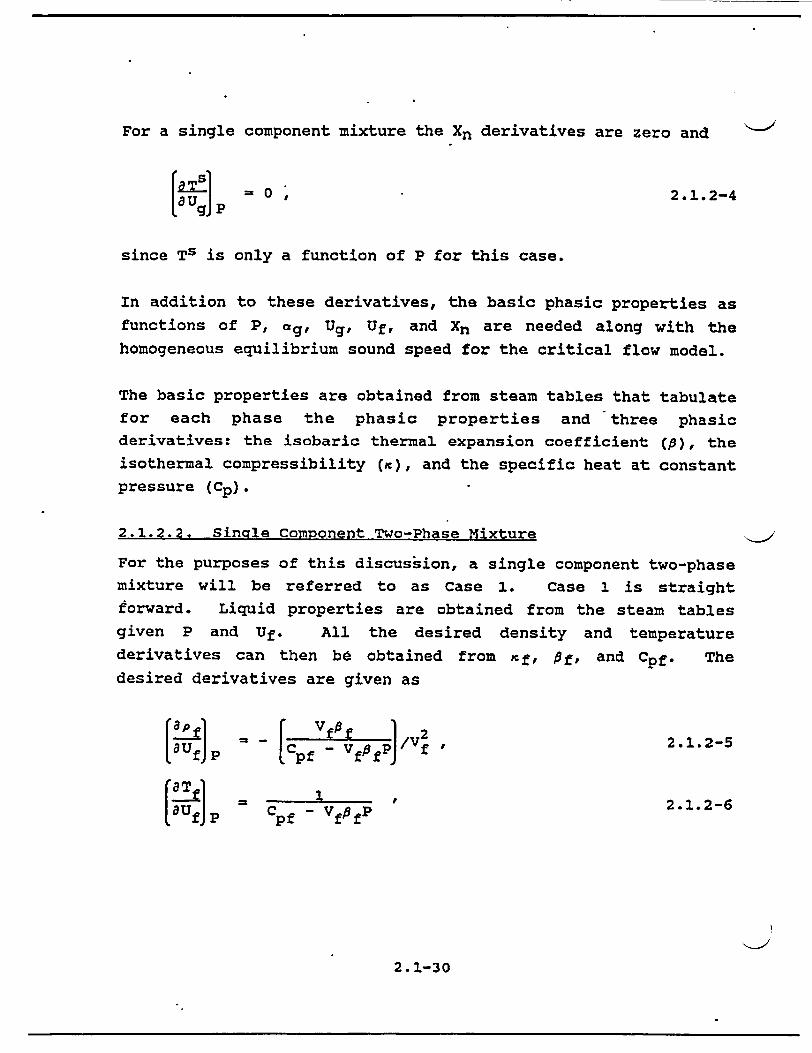
For a single component mixture the Xn derivatives are zero and

0 ,2.1.2-4

since Ts is only a function of P for this case.

In addition to these derivatives, the basic phasic properties as functions of P, ag, Ug, Uf, and Xn are needed along with the homogeneous equilibrium sound speed for the critical flow model.

The basic properties are obtained from steam tables that tabulate for each phase the phasic properties and three phasic derivatives: the isobaric thermal expansion coefficient (p), the isothermal compressibility (m), and the specific heat at constant pressure (Cp).

2.1.2.2. Single component Two-Phase Mixture

For the purposes of this discussion, a single component two-phase mixture will be referred to as Case 1. Case I is straight forward. Liquid properties are obtained from the steam tables given P and Uf. All the desired density and temperature derivatives can then be obtained from xf, 9f, and Cpf. The desired derivatives are given as

=OUfJp - p- VfPfJ-f , 2.1.2-5

rB 1 i PJ C pf- Vff1

L = C pf V f)fp21.-

2.1-30

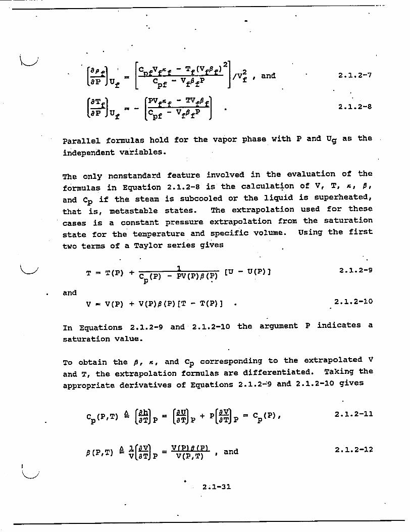
Capr-- f [ vfpf) [!ft [cv. Tf f] , / and 2.1.2-7

ap jUf - [Opf - vfTfP f Ua fU (Cpfr - Vf fP 2.1.2

Parallel formulas hold for the vapor phase with P and Ug as the

independent variables.

The only nonstandard feature involved in the evaluation of the

formulas in Equation 2.1.2-8 is the calculati.on of V. T, x, P,

and Cp if the steam is subcooled or the liquid is superheated,

that is, 'etastable states. The extrapolation used for these

cases is a constant pressure extrapolation from the saturation

state for the temperature and specific volume. Using the first

two terms of a Taylor series gives

T = T(P) + CI(P) - PV(P)C(P) [U - U(P)] 2.1.2-9

p

and

V = V(P) + V(P)P(P)[T - T(P)] 2.1.2-10

In Equations 2.1.2-9 and 2.1.2-10 the argument P indicates a

saturation value.

To obtain the ,, x, and Cp corresponding to the extrapolated V

and T, the extrapolation formulas are differentiated. Taking the

appropriate derivatives of Equations 2.1.2-9 and 2.1.2-10 gives

C (P,T) a

p!(P If)vi (v Pa (P ) , and 2.1.2-12

p(P,T) = VLaTJ P V(P,T) a

2.1-31

i(P,T) A - V-T = {V(P) + CT - T(P)]V(P)P(P)} V(P,T) -1_ (8 V T)- (Vp(P)V (P, T)

-[T - T(P)] V(P) dB(P + '2 (P) (P)/V(PT).

2.1.2-13

Equation 2.1.2-11 shows that a consistently extrapolated Cp is just the saturation value Cp(P). Equation 2.1.2-12 gives the

extrapolated p as a function of the saturation properties and the extrapolated V. Equation 2.1.2-13 gives the consistently

exptrapolated x as a function of the extrapolated and saturation

properties. The extrapolated x in Equation 2.1.2-13 involves a change of saturation properties along the saturation line. In

particular, dP (P) involves a second derivative of specific volume. Since no second-order derivatives are available from the

steam property tables, this term was approximated for the vapor

phase by assuming the fluid behaves as an ideal gas. With this

assumption the appropriate formula for the vapor phase x is

9g(PT) = (Vg(P) + [Tg - T(P)] Vg(P)Pg(P)) rcg(P)/Vg(PT).

2.1.2-14

For the liquid phase extrapolation (superheated liquid) only the

specific volume correction factor in Equation 2.1.2-13 was

retained, that is,

Kf(PlT) = Vf(P)C f(P) 2.1.2-15 Vf(PIT)

2.1-32

The homogeneous equilibrium sound speed is calculated from

standard formulas using the saturation x's, P's, and Cp's. The

sound speed formula

2 2 2 rz [ + - 2kd)] a2 1T X T g

+ (I X) T+Vf dP' 2.1.2-16

is used, where from the Clapeyron equation

dp__s h .. h dT T

TSV; - f

2 . 1 . 2-17

and X is the steam quality based on the mixture mass.

2.1.2.3. Two Coimnonent, Two-phase mixture

This case is referred to as Case 2. The liquid phasic properties

and derivatives are calculated in exactly the same manner as

described in Case 1 (see section 2.1.2.2), assuming the

noncondensible component is present only in the gaseous phase.

The properties for the gaseous phase are calculated assuming a

Gibbs-Dalton mixture of steam and an ideal noncondensible gas. A

Gibbs-Dalton mixture is based upon the following assumptions:

1. P = Pn + Ps 2.1.2-18

2. Ug = XnUn + (I - Xn)Us , and 2.1.2-19

t

2.1-33

3- XnVn (1 - Xn)VS Vg 2

where PS and Pn are the partial pressures of the steam and

noncondensible components, respectively. The internal energies Us, Un, and the specific volumes Vs, Vn are evaluated at the gas temperature and the respective partial pressures. The vapor properties are obtained from the steam tables and the noncondensible state equations area

PnVn - RnTg and

S O {CT + Uo U CoTg +-1 Do(Tg - To)2 + Uo

2.1.2-21

Tg < To

Tg a 0 2.1.2-22

Given P, Ug, and Xn, Equations 2.1.2-18 through 2.1.2-20 are solved implicitly to find the state of the gaseous phase. If

Equation 2.1.2-18 is used to eliminate Pn and Equation 2.1.2-21 is used for Vn, Equations 2.1.2-19 and 2.1.2-20 can be written as

(I -Xn)Us + XnUn [Tg(UsPS)l Ug= 0

nVs (Us' gs Pg

(- Xn T ,s) (P- P n T (UIPSS) s Xn~ns

g 9

2.1.2-23

2.1.2-24

Given P, Ug, and Xn, Equations 2.1.2-23 and 2.1.2-24 implicitly determine Us and Ps. (Equation 2.1.2-20 was divided by the temperature and multiplied by the partial pressures to obtain

Equation 2.1.2-24.)

aThe code input permits selection of any one of six noncondensible gases. The constants used to represent air are in SI units: To - 250.0 K, CO = 715.0 J/(kg/K), Uo = 158990.52 J/kg, Do = 0.10329 J/(kg K2), and Rn = 287.066 N m/(kg K).

2.1-34

and

2.1.2-20 -

To obtain the derivatives needed in the numerical scheme, the

derivatives of Us and Ps are taken with respect to P, Ug, and Xn.

These derivatives, can be obtained from Equations 2.1.2-23 and

2.1.2-24 by the use of the chain rule and implicit

differentiation.. For example, taking t~he derivative of Equations

2.1.2-23 and 2.1.2-24 with respect to P [recall that Ps

Ps(P,Ug,Xn) and Us - Us(P,Ug,Xn)] yields

(dU-1OT' 'Xn fldTguJ

-XnRn - (1- Xn)Rs

10 - X + T E R M

0 + TERM2

+ R + TERM1

(1 - Xn Rs

xaP J Ig,Xn

2.1.2-25

as a linear system of two equations determining

and 149 pa ' aP JUgXn an JUgXn

In Equation 2.1.2-25

= R s =T Tg 2.1.2-26

is the equivalent gas constant for the steam vapor,

"TE[S = (I -5)Pn-

- V v , ,u2.1.2-27

2.1-35

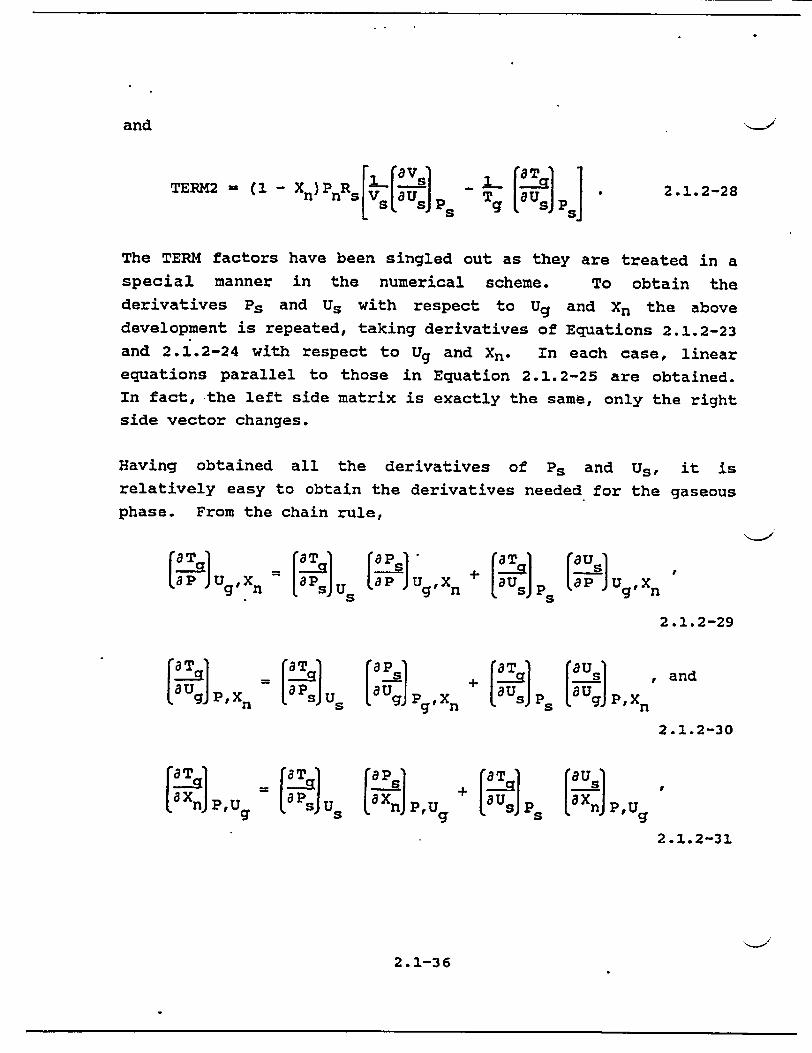
and

rr .1 faT 1 TERZ42=~ ~ (1X RI"I8 5 r(O 2.1.2-28 rl _lS vsLB ~ ~ T BUl5J•.•=_ TERM2' l-(I-Xn)Pnas It Mal SJ - Tg I Cs U. • S

The TERM factors have been singled out as they are treated in a special manner in the numerical scheme. To obtain the derivatives Ps and Us with respect to Ug and Xn the above development is repeated, taking derivatives of Equations 2.1.2-23 and 2.1.2-24 with respect to Ug and Xn. In each case, linear equations parallel to those in Equation 2.1.2-25 are obtained. In fact, the left side matrix is exactly the same, only the right side vector changes.

Having obtained all the derivatives of Ps and Us, it is relatively easy to obtain the derivatives needed for the gaseous phase. From the chain rule,

CMT1 a a aPI I rain aPJ UgXn iaPSJus tP JUgIXn + sP( s taP j UgIn

2.1.2-29

[p OT1(a au an OTPgj'xn lipsjus lgJpx+P9 n as P• PXn

2.1.2-30

( T 1 faT 1 +'8[a TrOT -a u5 [2I f 1.2 BXnJ ~ :[ 5 s~u [XnlJ>,Ug + [sl~ a-x~>U

2.1.2-31

2.1-36

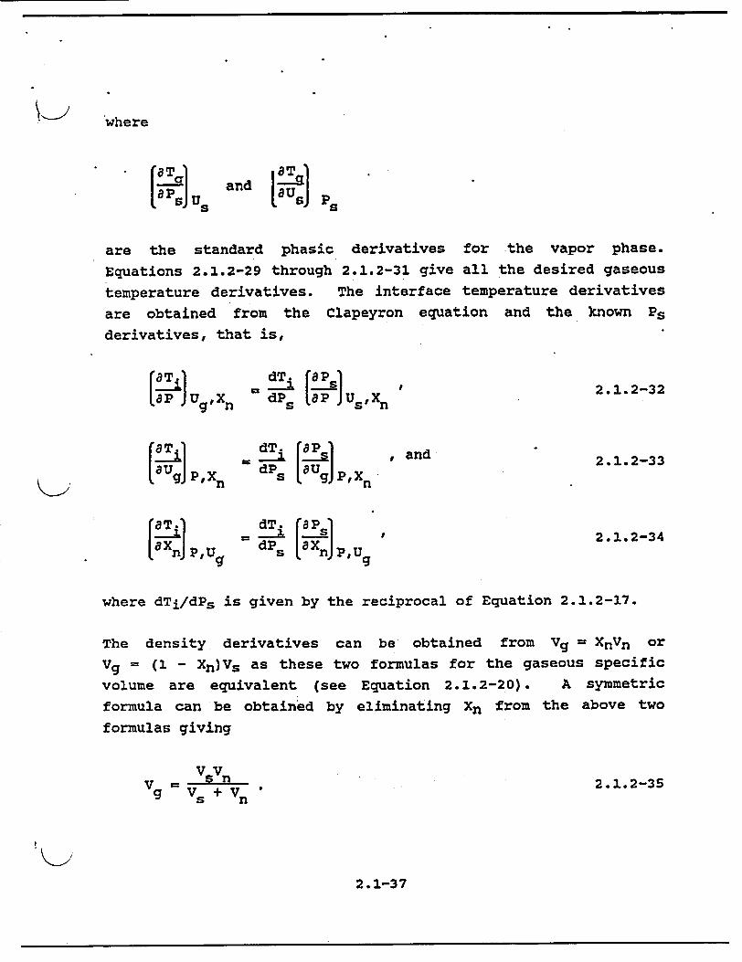
BPsJ Us a I

are the standard phasic derivatives for the vapor phase.

Equations 2.1.2-29 through 2.1.2-31 give all the desired gaseous

temperature derivatives. The interface temperature derivatives

are obtained from the Clapeyron equation and the known Ps

derivatives, that is,

T Jui dsT (aP s, lap JUgOVXn dPs lap J u51Xn

2.1.2-32

(UgJ PXn

dT. ra PdP5 Ogp,

S [agj~ n'

, and 2.1.2-33

( T.dT. [rnPn5 ' PX CJ= dP s I O nJp PU

2.1.2-34

where dTi/dPs is given by the reciprocal of Equation 2.1.2-17.

The density derivatives can be obtained from Vg = XnVn or

Vg = (1 - Xn)Vs as these two formulas for the gaseous specific

volume are equivalent (see Equation 2.1.2-20). A symmetric

formula can be obtained by eliminating Xn from the above two

formulas giving

vvn V = V+ Vn. g VIS+ Vn

2.1.2-35

2.1-37

where

t

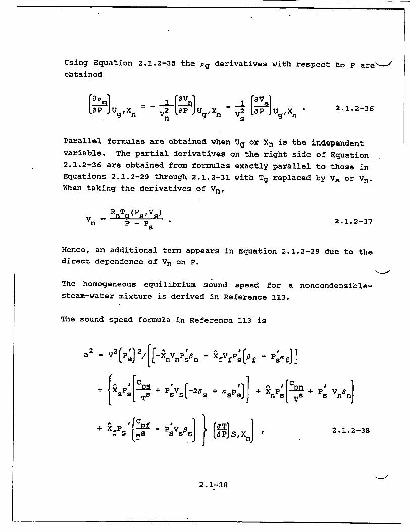
Using Equation 2.1.2-35 the pg derivatives with respect to P are"- 1

obtained

(~ ~ 2 (:g1 alrVn1 B P~gX~- 2 'pJ Ug IXn - v. LB'pJUg'Xfl2.1.2-36

Parallel formulas are obtained when Ug or Xn is the independent variable. The partial derivatives on the right side of Equation 2.1.2-36 are obtained from formulas exactly parallel to those in Equations 2.1.2-29 through 2.1.2-31 with Tg replaced by Vs or Vn. When taking the derivatives of Vn,

Vn = RnT (Ps Vs) P -Ps 2.1.2-37

Hence, an additional term appears in Equation 2.1.2-29 due to the direct dependence of Vn on P.

The homogeneous equilibrium sound speed for a noncondensiblesteam-water mixture is derived in Reference 113.

The sound speed formula in Reference 113 is

A2 ) V-- ] VfP(f- 6

+ XsP's + PV 5 (-2Ps + XsPs + XnPs 's + PS Vn}

A C I 1 # 1 P.....

+ P l RjP. I-T: - Ipvp I j 2.1.2-38

2.1-38

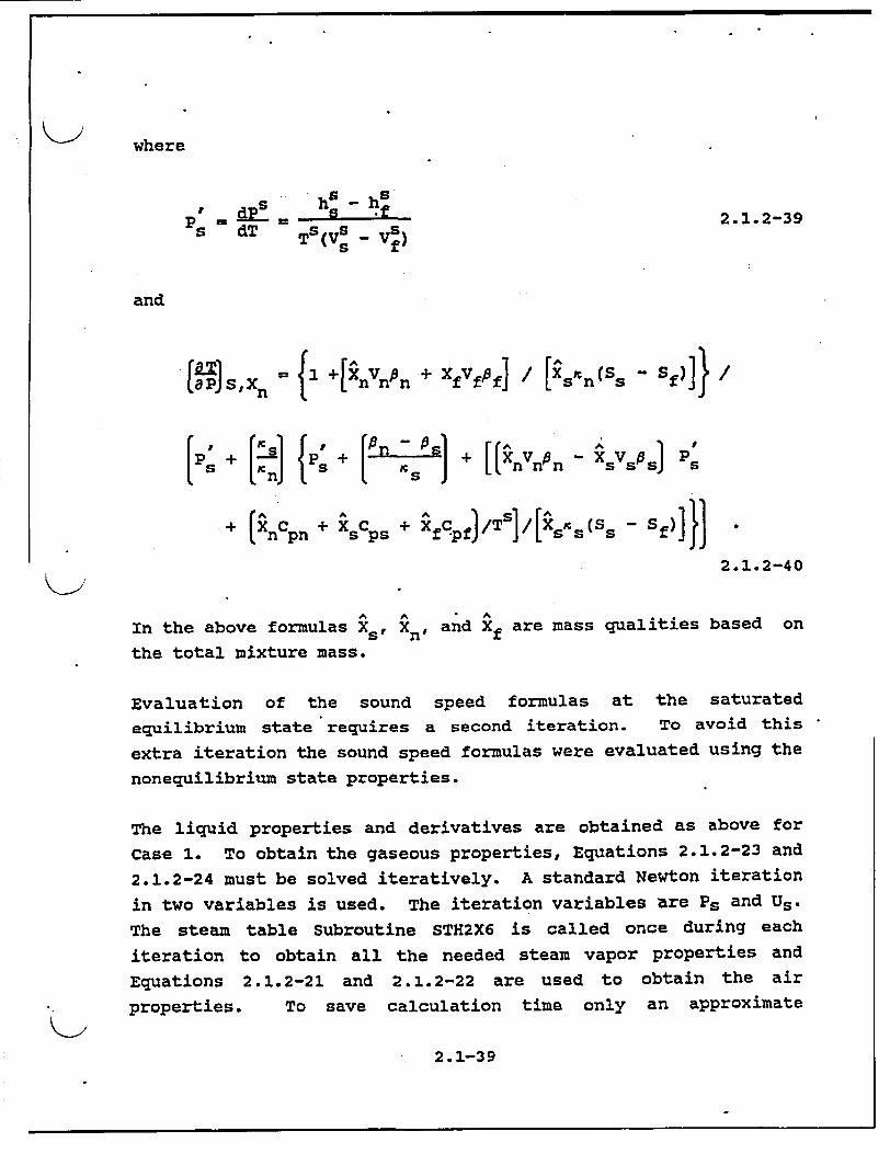
where

S h dp hs - .f__2123 P 2.1.2-39

s dT T s(V - V'-)

and

aLp S. Xn= f +[XnVnfn + XfVf f] P / Xs- Sf)]} /

.0 114 + [(A° Avo .4 Ps + fps + [ s + XnVn] n - Xs + s[p s

+ (ncpn + s~ps + XfcPf) /Ts]/ X sics(sS - Sf)]}

2.1.2-40

A A A

In the above formulas Xs, Xn, and Xf are mass qualities based on

the total mixture mass.

Evaluation of the sound speed formulas at the saturated

equilibrium state requires a second iteration. To avoid this

extra iteration the sound speed formulas were evaluated using the

nonequilibrium state properties.

The liquid properties and derivatives are obtained as above for

Case I. To obtain the gaseous properties, Equations 2.1.2-23 and

2.1.2-24 must be solved iteratively. A standard Newton iteration

in two variables is used. The iteration variables are Ps and Us.

The steam table Subroutine STH2X6 is called once during each

iteration to obtain all the needed steam vapor properties and

Equations 2.1.2-21 and 2.1.2-22 are used to obtain the air

properties. To save calculation time only an approximate

2.1-39

Jacobian is used inside the iteration loop. From Equation 2.1.2-24, it is clear that if the steam behaves as an ideal gas, that is, Rs = (VsPs/Tg) is constant, then Equation 2.1.2-24 is a simple linear equation determining Ps directly in terms of P and Xn. It simplifies the iteration to neglect the derivatives of Rs in the Jacobian, making it equal the left side matrix in Equation 2.1.2-25, with TERM1 and TERM2 terms absent. This iteration has been tested with Ps ranging from 2000 Pa to P and has always converged. The iteration is terminated when IaPsl/P and IA7Vs/Vg are both <0.0005. Hand calculations have been performed to compare both. the properties and derivatives with the code calculations. In all cases the scheme converged in 4 iterations or less.

once the iteration has converged the gaseous properties are determined from the formulas in this section. In the evaluations of all these derivatives the full matrix in Equation 2.1.2-25 is used including TERM1 and TERM2.

2.1-40

K>

2.1-41

2.1.3. Constitutive Models

The constitutive relations include models for defining flow

regimes and flow regime related models for interphase drag, wall

friction, heat transfer, interphase heat and mass transfer,

horizontal and vertical stratification, and water packing

mitigation.

2.1.3.1. Flow Regime Maps

In RELAP5 the constitutive relations include flow regime effects

for which simplified mapping techniques have been developed to

control the use of constitutive relation correlations. Three

flow regime maps are utilized. They are vertical and horizontal

maps for flow in pipes, and a high mixing map for flow in pumps.

The flow regime maps are based on the work of Taitel and

Dukler 2 7 , 2 8 and Ishii. 2 9 - 3 1

Taitel and Dukler have simplified flow regime classification and

developed semi-empirical relations to describe flow regime

transitions. However, some of their transition criteria are

complex and further simplification has been carried out in order

to apply these criteria efficiently in RELAPS. In addition,

post-CHF regimes as suggested by Ishii 2 9 are included.

Vertical Flow Reaime Map

The vertical flow regime map is modeled as seven regimes, three

of which are for pre-CHF heat transfer, three of which are for

post-CHF heat transfer, and one of which is for vertical

stratification. For pre-CHF heat transfer, the regimes modeled

are the bubbly, slug, and annular mist regimes. Formulations for

these three regimes were utilized by Vince and Lahey 3 2 to analyze

their data. For post-CHF heat transfer, the bubbly, slug, and

annular mist regimes are transformed to the inverted annular,

inverted slug, and mist regimes, respectively, as suggested by Ishii. 2 9 Unheated components are also modeled utilizing the preCHF map. A schematic representing the pre- and post-CHF regimes of the vertical flow regime map is shown in Figure 2.1.3-1. The vertically stratified regime may exist at low flow conditions and a schematic showing its relationship in the vertical flow regimemap is given in Figure 2.1.3-2. The criteria for defining the boundaries for transition from one regime to another are given by the following correlations.

Increasing ag (VOIDG)

Pre-CHF region

Post-CHF region

I08 - S I

OS-A I

Figure 2.1.3-1. Sketch of Vertical Flow Regime Map.

For the bubbly to slug transition, Taitel and Dukler 2 7 , 2 8

suggested that bubbly flow may not exist in tubes of small diameter where the rise velocity of small bubbles exceeds that of Taylor bubbles. The small bubble rise velocity is given by the correlation2 8

Vsb = 1.53 g(pf - Pg)a/Pf 2 j 1/4 2.1.3-1

and the Taylor bubble rise velocity is given by the correlation1 1

VTb = 0.35 1 gD(pf - pg)/Pf ) 1/2 2.1.3-2

2.1-42

I I Bubbly Slug Annular-mist (BBY) (SLG) I (ANM) I I

-. . . . . . . . 1" . . . . " " . . ... "

I i. Inverted Inverted IMist annular I slug IMit

(IAN) f (ISL) Q (MST) I I

I n ! I

Bubbly Annular Slu mist i I I I

3000 . --aBS aS_-A

Transition

-. 2000 T0

- I I

uI Annular Bubbly Slug I mist

I ! I I

"B-S aS-A

Transition

Vertically stratified flow 0

Void (ag)

Figure 2.1.3-2. Vertical Flow Regime Map Including the Vertically Stratified Regime.

2.1-43

(Note: in Reference 28, pf - pg is approximated as pf, see also•

References 30 and 33). Accordingly, the limiting tube diameter

allowing the presence of bubbly flow is

D* Z 19 , 2.1.3-3

where D* is the dimensionless tube diameter,

D* = D[g(pf - pg)/ ]I 21. 2.1.3-4

Equation 2.1.3-2 is the dimensionless ratio of tube diameter to

film thickness times the Deryagin number, where the Deryagin number is the ratio of film thickness to capillary length. Also, in the limit, as the fluid properties approach the thermodynamic

critical pressure, D* = D.

For tubes with diameters satisfying the condition of Equation 2.1.3-3 the bubble-slug transition occurs at a void fraction ag -- '

0.25 for low mass fluxes of G < 2000 kg/m 2 s. By combining this void criterion with Equation 2.1.3-3 the bubble-slug transition

criterion can be defined such that

- 8] L = 0.25 MIN [1.0, (D*/19) ] . 2.1.3-5

V Hence, if the local void fraction, ag, exceeds the criterion of

Equation 2.1.3-5 then bubbly flow cannot exist since the rise

velocity of small bubbles exceeds that of Taylor bubbles. The

exponential power of 8 is used to provide a smooth variation of

aL as D* decreases.

At high mass fluxes of G > 3000 kg/m 2 s, bubbly flow with finely

dispersed bubbles can exist up to a void fraction, ag, of 0.S.

Then, if the criterion is linearly interpolated between the upper

2.1-44

) and lower void limits, the bubbly-slug transition criterion can be written is

B-S L 2.1.3-6

for mass fluxes of G < 2000 kg/m 2 s,

"a B-S = aL + 0.001 (G - 2000)(0.5 - aL) 2.1.3-7

for mass fluxes of 2000 < G < 3000 kg/m2 s, and

RB-S =0.5 2.1.3-8

for mass fluxes of G k 3000 kg/m2 s. The flow regime can

therefore be in the bubbly regime if a < QB-S and in the slug

regime if a 9 aB-S

The bubble-slug transition defined by Equations 2.1.3-6 to 2.1.3

8 is similar to that given by Taitel and Dukler, 2 8 except that

the void fraction relation is converted into a form based on

liquid and vapor superficial velocities and finely dispersed

bubbles are also distinguished from ordinary bubbles.

For the slug to annular flow transition, Taitel and Dukler 2 8

developed a criterion based on the critical vapor velocity

required to suspend a liquid droplet. The critical velocity, Uc,

is written as

uc - 3 .l[1g(pf - Pg)] 1 / 4 / P / 2 (agvg)c" 2.1.3-9

The value 3.1 for the numerical coefficient is somewhat larger

than the value of-1.4 reported by Wallis 3 4 but is a better fit to

the data reported by Vince and Lahey. 3 2 In comparing RELAP5 code

results to data, however, the coefficient value of 1.4 gives

better results. The void fraction must also be greater than 0.75

2.1-45

in order to get good comparisons between code results and data.

Hence, solving Equation 2.1.3-9 for void fraction and imposing a"-'

lower void limit of 0.75 yields the slug to. annular transition criterion for which

Ss-A M MAX 0.75, 1. 4 [og(pf - pg) 1 /4/(VgP 1/2 2.1.3-10

where the flow regime is said to be in the slug regime if

ag 9 : S-A and in the annular-mist regime if a g > aS-A"

For post-CHF heat transfer the same formulations are used to define the inverted flow regime transition criteria in that Equations 2.1.3-6 through 2.1.3-8 also define the inverted slug regime transition and Equation 2.1.3-10 defines the inverted slug to mist regime transition.

At low mass fluxes the possibility exists for vertically stratified conditions. In RELAP5 vertical flow in a volume cello

is considered to be stratified if the difference in void fraction

of the volumes above and below is greater than 0.5 and if the magnitude of the volume average mixture mass flux is less than the Taylor bubble rise velocity mass flux. The Taylor bubble criterion is based on the Taylor bubble velocity given by Equation 2.1.3-2 such that

JGI < p VTb 2.1.3-11

where vTb is the Taylor bubble velocity and

JGI = lagPgVg + afpfvfI . 2.1.3-12

Hence, if Equation 2.1.3-11 is true, then transition to vertical stratification exists and if Equation 2.1.3-11 is false, then

transition to vertical stratification does not exist.

Rev. 1 2.1-46 10/88"

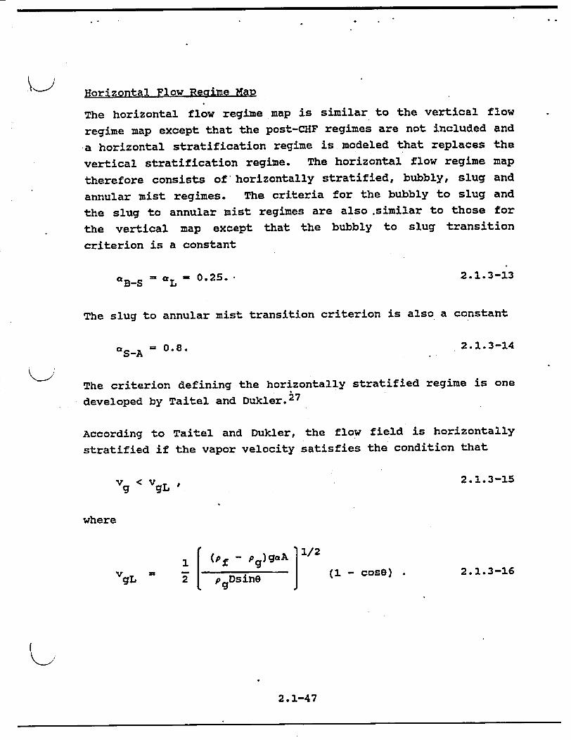
Horizontal Flow Regime MaR

The horizontal flow regime map is similar to the vertical flow

regime map except that the post-CHF regimes are not included and

a horizontal stratification regime is modeled that replaces the

vertical stratification regime. The horizontal flow regime map

therefore consists of horizontally stratified, bubbly, slug and

annular mist regimes. The criteria for the bubbly to slug and

the slug to annular mist regimes are also .similar to those for

the vertical map except that the bubbly to slug transition

criterion is a constant

"B-S L - 0.25. 2.1.3-13

The slug to annular mist transition criterion is also a constant

CS-A = 0.8. 2.1.3-14

The criterion defining the horizontally stratified regime is one

developed by Taitel and Dukler. 2 7

According to Taitel and Dukler, the flow field is horizontally

stratified if the vapor velocity satisfies the condition that

vg < vgL , 2.1.3-15

where

SP Of - )gaA 11/2

(I - cose) 2.1.3-16

K>

2 . 1-47

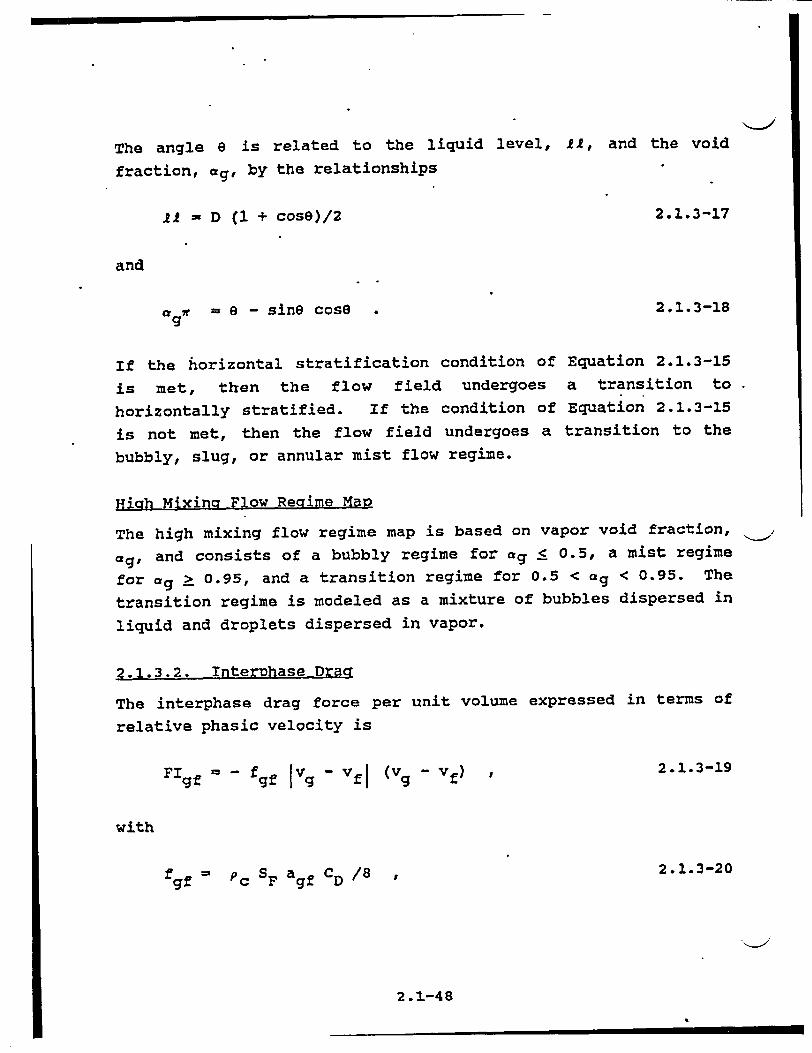
The angle e is related to the liquid level, 21, and the void

fraction, ag, by the relationships

22 =D (I + cose)/2 2. 1.3-17

2.1•3-18ag7 = a - sine cose .

If the horizontal stratification condition of Equation 2.1.3-15

is met, then the flow field undergoes a transition to

horizontally stratified. If the condition of Equation 2.1.3-15

is not met, then the flow field undergoes a transition to the

bubbly, slug, or annular mist flow regime.

High Mixing Flow Regime May

The high mixing flow regime map is based on vapor void fraction,

ag, and consists of a bubbly regime for ag • 0.5, a mist regime

for ag > 0.95, and a transition regime for 0.5 < ag < 0.95. The

transition regime is modeled as a mixture of bubbles dispersed in

liquid and droplets dispersed in vapor.

2.1.3.2. Interphase Dra=

The interphase drag force per unit volume expressed in terms of

relative phasic velocity is

FIgf = - ff IVg- vfj (Vg- vf) 2.1.3-19

with

2.1.3-20fgf = PC SF agf CD / 8

2.1-48

and

where

PC density of the continuous phase,

CD = drag coefficient,

agf = interfacial area per unit volume, and

SF - shape factor.

The shape factor3 0 , SF, is assumed to be unity (1.0). The

evaluation of agf and CD for different flow regimes is covered in

the following discussion.

DpDsersed Fl0w

The bubbly and mist flow regimes are both considered as dispersed

flow. According to Wallis 3 4 and Shapiro, 3 5 the dispersed bubbles

or droplets can be assumed to be spherical particles with a size

distribution of the Nukiyama-Tanasawa form. The Nukiyama

Tanasawa distribution function in nondimensional form is

p* = 4d* 2 e-2d* 2.1.3-21

where d* = d/d'; d' is the most probable particle diameter, and p* is the probability of particles with a nondimensional diameter

of d*. With this distribution, it can be shown that the average

particle diameter do - 1.5 d', and the surface area per unit

volume is

a - a d* p* d__* -2. , 2.1.3-22 d.3 p* dd*

2.1-49

where = = ag for bubbles and a = af for droplets. In terms of the

average diameter, do, the interfacial area per unit volume, agf,

is

agf =3.6a/d . 2.1.3-23

The average diameter do is obtained by assuming that do - 1/2

dmax. The maximum diameter, dmax, is related to the critical

Weber number, We, by

We = dmax Pc(vg - Vf) 2 /C' 2.1.3-24

The values for We are presently taken as We = 10 for bubbles and

We = 3.0 for droplets.

The drag coefficient is given by Ishii and Chawla 3 0 for the

viscous regime as

C = 24(1 + 0.1 Re 0 7 5 )/Re D p p

2.1.3-25

where the particle Reynolds number Rep is defined as

Rep = 1 Vg - Vfj do pcm "2.1.3-26

The mixture viscosity, pm, is pm = pf/af for bubbles and ym / (a ) 2.5 for droplets.

2.1-50

p.i...,. .... L I,,- -0"o _ ,",-o VT

lo~eoooo o ee

0 90. •"% S:- • :

SOverall average =

void fraction - ag

&-- ags

Figure 2.1.3-3. Slug Flow Pattern

slug~ Flow

Slug flow is modeled as a series of Taylor bubbles separated by

liquid slugs containing small bubbles. A sketch of a slug flow

pattern is shown in Figure 2.1.3-3. The Taylor bubble has a

diameter nearly equal to the pipe diameter and a length varying

from one to one hundred pipe diameters.

The total drag in slug flow is partitioned into small bubble and

Taylor bubble drag components:

fgf = (fgf)sb + (fgf)T 2.1.3-26.1

The interphasic friction term for small bubbles, (f )_sb, is of

the form given in Equation 2.1.3-20 and is determined with the

agf and CD derived for dispersed flow (Equations 2.1.3-23 and

2.1.3-25).

Rev. 2 8/922.1-51

-H

\

[

The void fraction of a single Taylor bubble, %,' in the total ,> mixture is

ab = (g- ags/ a gs) • 2.1.3-27

where a is the average void fraction in the liquid film and gs slug region.

To provide a smooth transition into and out of slug flow, ag , in Equation 2.1.3-27, is considered as a free parameter varying from the void fraction (aBS) at the bubbly to slug flow regime transition to nearly zero at the slug to annular mist flow regime transition. The variation is represented by the exponential

expression

ags = aB_S exp[- 10(ag - aBS)/('S-aBS)] 2.1.3-28

Three options are available for computing the Taylor bubble interphase drag in slug flow: the base INEL drag, the Wilson drag, and the B&W modified slug-drag model. The Wilson drag is based on the Wilson bubble rise velocity in a vertical pipe. 1 3 5

The BWNT modified slug-drag model uses coefficients that are a function of pressure and void fraction to adjust the' INEL drag. model. The default is the INEL model.

INEL Drag Model

By approximating the ratio of the Taylor bubble diameter to the tube diameter and the diameter-to-length ratio of a Taylor bubble, Ishii and Mishima31 obtained the surface-to-volume ratio of a Taylor bubble as 4.5/D. In the INEL drag model, this is used to obtain the interfacial area per unit volume, agf, for

slug flow:

Rev. 3 2.1-52 10/92

agf = (4.5 Ct/D)ab + (3.6 &gs/d0 )(i - ab) 2.1.3-29

in which the first term pertains to Taylor bubbles and the second

term to small bubbles. Ct is a roughness parameter that is

introduced to account for irregularities in the surface of large

Taylor bubbles. At the present time, Ct is assumed to be unity (1.0).

The INEL model drag coefficient for Taylor bubbles is given by

Ishii and Chawla30 as

(CD)T = 9.8 (1 - b) 2.1.3-30

where ab is given by combining Equations 2.1.3-27 and 2.1.3-28.

The Wilson Drag Model

K-> -The Wilson drag model was first derived for reflood applications 136.

using BEACH and is now applied to non-reflood conditions in

RELAP5/MOD2-B&W.

b,c,d,e

Rev. 3 2.1-52.1 10/92

bcde

The estimate of the phasic slip, Av, is obtained from a modified set of the Wilson 1 3 5 bubble rise model:

-1

b.cde

Itev. 3 2.1-52.2 10/92

The coefficients a and b for j 2 I and 2 are from the original

correlation. The third set (j = 3), however, was added to obtain

a better match to the original data at high a* (greater than

about 6.526).. As implemented in REIAP5/MOD2-B&W, the bubble

velocity is multiplied by a user-defined multiplier, CWB:

vbub = CWB AV. 2.1.3-30.6

b,c,d,e

where CWSL is a user-defined multiplier for slug flow conditions

which, at the present time, is set equal to one.

In RELAPS; an interphase drag for each volume is calculated and

then the drag for the junctions between connecting volumes are

determined. RELAP5 uses several techniques to smooth the void

behavior across the junction. One of these smoothing techniques

is used when the difference between the void fractions of

adjoining volumes is greater than 0.001. For some situations

(for example, in RSG PWR small break LOCA, during the hot leg

draining period and during the period preceding core uncovery),

it is expected that discontinous void behavior will occur at the

core-upper plenum boundary. The unmodified junction drag logic

calculates void behavior reasonably well. However, because

REL&P5 smooths the void behavior across the junction when the

difference between connecting nodes is greater than 0.001, a flat

Rev. 2

2.1-52.3 8/92

void profile is calculated for some cases as illustrated in•,

Figure 2.1.3-3.1. Therefore, as an option to the Wilson drag

model, the void difference threshold for curve smoothing is

increased to 0.5.

U

Cwuv#

COME ELEVATICA

Figure 2.1.3-3.1. Typical RELAP5 Void Profile: Smoothed and Unsmoothed Curves.

BWNT has added an option to adjust the slug interphase drag for

non-reflood applications via coefficients added to Equation

2.1.3-26.1. The adjustments, based on numerous benchmarks, are

functions of pressure and void fraction as shown in the following

equations.

fgf = Mst [(fgf)sb + Ms (fgf)T I

b,cpd,e

2.1.3-30.7.1r

]Rev. 3

10/922.1-52.4

where

LI

b,c,d,e

The values given in parentheses are the default coefficients.

These are selected by the user through input of a control volume

flag which refers back to a tabular default table number

containing the five coefficients that are listed. A different

set of coefficients may be specified by the user on input. Use

of the default drag adjustments are appropriate for two-phase

applications in heated tube bundles and small diameter pipes

during non-reflood calculations.

Annular Mist Flow

Annular mist flow is characterized by a liquid film along the

,wall and a vapor core containing entrained liquid droplets. The

INEL drag is the sum of the annular vapor and liquid droplet drag

components

fgf = (fgf)ann + (fgf)drp. 2.1.3-30.8

Let aff be the average liquid volume fraction of the liquid film

along the wall. Then, from simple geometric considerations, the

interfacial area per unit volume can be shown to be

Rev. 3

241-52.5 10/92

agf = (4Can/D) (1 - aff) /2 + ( 3 . 6 afd/do)(l - mff), 2.1.3-31

where Can is a roughness parameter introduced to account for waves in the liquid wall film and cfd is the average liquid volume fraction in the vapor core, for which

afd = (af - aff)/(l - aff) . 2.1.3-32

A simple relation based on the flow regime transition criterion and liquid Reynolds number is used to correlate the average liquid film volume fraction. For vertical flow regimes, the entrainment relation is

aff ,a fC f exp {-7.5 * 10-5 (cgvg/uc)6 ) 2.1.3-33

where uc is the entrainment critical velocity given by Equation '

2.1.3-9 with the coefficient 3.1 replaced by 1.4. For horizontal flow regimes, the entrainment relation is

a = fCf exp 1-4.0 . 10-5 (vg/Vg 1 ) 6 }, 2.1.3-34

where v g is the horizontal stratification critical velocity given by Equation 2.1.3-16. The term C is expressed as

f

C f 0 4pf fVf D/ Pf

Rev. 3 10/922.1-52.6

The interfacial friction factor, fi' for the liquid film takes

the place of CD in Equation 2.1.3-20, and is described by a

correlation obtained by Bharathan et al. for which

fi = 4 (o.oo5 + A(6*)B ) , 2.1.3-35

- -0.56 + 9.07/D*, 2.1.3-36

2.1.3-37W 1.63 + 4.74/D*, and

1/22.1.3-38

= { (P�- Pq) g o

The term 6* is the liquid wall film Deryagin number for which 6

is the film thickness, and D* is the dimensionless diameter given

by Equation 2.1.3-5.

BWNT has added an option to include a multiplicative coefficient

on the overall drag computed for control volumes in an annular

mist flow regime. This coefficient is available for non-reflood

applications. The default coefficient, xms, is 1.0; however, it

may be changed on input specified by the user. The coefficient

is applied as follows

fgf = xms [(fgf)ann + (fgf)drp] 2.1.3-38.1

Rev. 2 8/922.1-53

where

log1 0 A

B

6*

Vertical Stratified Plow

For vertically stratified flow the previously discussed

interphase drag relationships are applied except that a low

interphase drag coefficient of 0.1 N-s2/M5 is imposed for the

junction above the vertically stratified volume.

Horizontal stratified Flow

By simple geometric consideration, one can show that the

interfacial area per unit volume is

agf -=4Cst sin 0 (ED) , 2.1.3-3§

where Cst is a roughness parameter introduced to account for

surface waves and is set to 1 at the present time.

The interface Reynolds number is defined with the vapor

properties and regarding liquid as the continuous phase for which

Rei = Di Pg I vg - vM "g , 2.1.3-40

where the equivalent wetted diameter, Di, for the interface is

D = c- rD/(e + sinG) . 2.1.3-41

The interfacial friction factor, fi, replaces CD in Equation

2.1.3-20 and is obtained by assuming typical friction factor

relationships for which

2.1.3-42fi = 64/Rei

Rev. 2 8/922.1754

for laminar flow, where Rei S 1187,

= ~~0.25 21*34 fl" 0.3164/Ref 2.1.3-43

for turbulent flow, where Rei 2 4000, and

fi = 0.0539 2.1.3-44

for the laminar to turbulent transition where 1187 < Rei < 4000.

Inverted Flow Recimes

The interphase drag relationships for post-CHF inverted flow

regimes are treated in a similar fashion to the corresponding

pie-CHF flow regimes except that the roles of vapor and liquid

are interchanged.

2.1.3.3. Wall Friction

In RELAP5, the wall friction force terms include only wall shear

effects. Losses due to abrupt -area change are calculated using

mechanistic form loss models. other losses due to elbows or

complicated flow passage geometry are modeled using energy loss

coefficients that must be. input by the user.

In the development of the RELAPS/MOD2 wall friction model,

emphasis was placed on obtaining reasonable values for wall

friction in all flow regimes. The flow regime models are

discussed in section 2.1.3.1.

The wall friction model is based on a two-phase multiplier

approach in which the two-phase multiplier is calculated from the

Heat Transfer and Fluid Flow Service (HTFS) modified Baroczy

correlation.37 The individual phasic wall friction components

are calculated by apportioning the two-phase friction between the

2.1-55

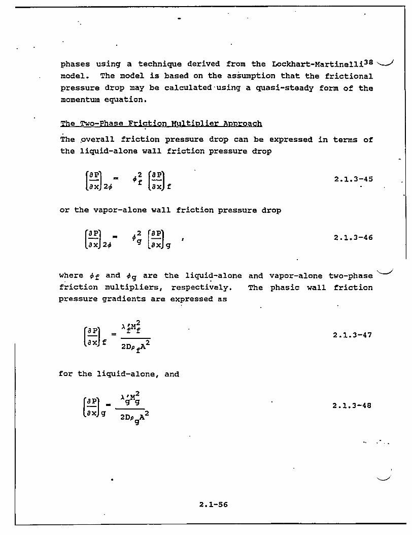
phases using a technique derived from the Lockhart-Martinelli 3 8

model. The model is based on the assumption that the frictional

pressure drop may be calculated using a quasi-steady form of the

momentum equation.

The Two-Phase Friction Multiplier Approach

The overall friction pressure drop can be expressed in terms of the liquid-alone wall friction pressure drop

a)20 4 P f r th ) 2ora w IIts

or the vapor-alone wall friction pressure drop

ap = 2 [aPi g

2.1.3-45

2. 1.3-46

where ýf and Sg are the liquid-alone and vapor-alone two-phase

friction multipliers, respectively. The phasic wall friction

pressure gradients are expressed as

-2 A 2

(!_X)f 2Dp fA22.1.3-47

for the liquid-alone, and

-I a ( axJ g

A 'M2

gg 2DpgA2 2.1.3-48

2.1-56

for the vapor-alone, where the prime indicates the liquid and

vapor-alone friction factors, respectively, calculated at the

respective Reynolds numbers

2.1.3-49Re, = OfP~fIVf D

ff

and

Re. - gPgIVgID

9 A g

2.1.3-50

The liquid and vapor mass flow rates, respectively, are defined

as

M f- fPfvfA 2.1.3-51

and

M =a p vA . 2.1.3-52

g ggg

Throughout the current literature the overall two-phase friction

pressure gradient is calculated using two-phase friction

multiplier correlations. However, regardless of the correlation

used, the multipliers may be interrelated using Equations 2.1.3

45 through 2.1.3-48 and the Lockhart-MartineJli 3 8 ratio defined

as

dP )f 2 dxj xd CX

9g2

Of2

2.1.3-53

2.1-57

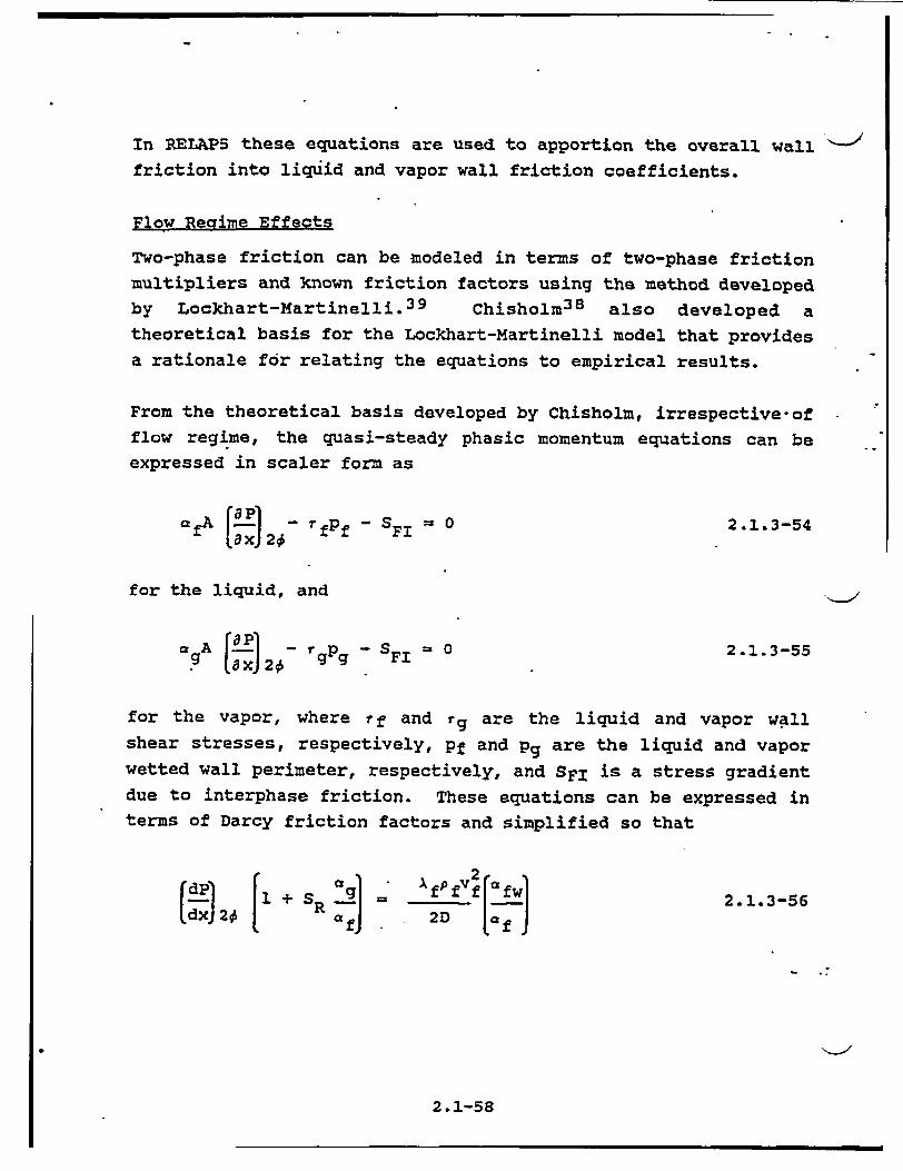
In RELAP5 these equations are used to apportion the overall wall

friction into liquid and vapor wall friction coefficients.

Flow Regime Effects

Two-phase friction can be modeled in terms of two-phase friction multipliers and known friction factors using the method developed by Lockhart-Martinelli. 3 9 Chisholm3 8 also developed a theoretical basis for the Lockhart-Martinelli model that provides a rationale for relating the equations to empirical results.

From the theoretical basis developed by Chisholm, irrespective-of flow regime, the quasi-steady phasic momentum equations can be expressed in scaler form as

2A ap fPf - S = 0 (;_XJ 20 F

for the liquid, and

=gA (a 1 p - SF1 = 0 g ITxJ 2# rgg Ft

2.1.3-54

2.1.3-55

for the vapor, where rf and rg are the liquid and vapor wall shear stresses, respectively, pf and pg are the liquid and vapor wetted wall perimeter, respectively, and SFI is a stress gradient

due to interphase friction. These equations can be expressed in terms of Darcy friction factors and simplified so that

2.1.3-56(dPl C,+ Og - Xfpfv,: x 0 fJI 2D

2.1-58

����1

for the liquid, and

2.1.3-57dPI (1 + SR) - A gPgVg2 ldx-J20 2D [-a9

for the vapor, where the interphase friction term, SR, is defined

as

= S F1 SR =

g LaxJ 2#

2.1.3-58

The terms afw and agw are the liquid and vapor volume fractions,

respectively, at the wall, and of and ag are the overall liquid

and vapor volume fractions, respectively. Taking the ratio of

Equation 2.1.3-56 to 2.1.3-57 gives

Z2 =v

[a g

1 + SR 9f

(1 - SR)

2.1.3-59

Consider the pure liquid case where ag = 0 and afw = of and for

which Equation 2.1.3-56 reduces to

(a r8(aPI 1 2 11 C• xif

AfP V2

2D2.1.3-60

For this case, the friction factor, xf, can be precisely

calculated based on a Reynolds number expressed in terms of D.

2.1-59

Similarly, for the two-phase case, liquid and vapor friction

factors can be calculated based on Reynolds number of

(_af - DjvflI Rf = f

'ifand 2.1.3-61

P g ( .Dlvi Rg. - '

P g 2.1 3-62

for the liquid and vapor, respectively. These terms have the property that, as one phase or the other disappears, the friction factors calculated reduce to their single-phase formulations.

Equations 2.1.3-56 and 2.1.3-57 can be rewritten as

. 2

2 D L tf

A V2

=2 2D

2.1.3-63

2.1.3-64-aI al

for the liquid and vapor, respectively. However, these equations are now flow regime dependent since knowledge of the wetted wall and overall void fractions is required in order to calculate the friction factors. The term Z2 can also be considered as a correlating factor relating the overall two-phase friction pressure gradient to the known phasic friction factors.

2.1-60

[dp 2)

and

[;~p 2

The quasi-steady phasic momentum equations similar to Equations

2.1.3-63 and 2.1.3-64 can also be written in terms of the RELAPS

friction coefficient, where

P [f f] P'WF (a fp fvf) 2.1.3-65

[dj2# a 9 + af 2,

for the liquid, and

g [dý 1 f = FWG(cgp Vg) 2.1.3-66

1dxJ206a + CtjZJ

for the vapor. Taking the sum of these two equations gives the

overall quasi-steady two-phase pressure gradient as

C) 21 FWF(afpfvf) + FWG(a gPgVg) . 2.1.3-67

It should be noted that the calculation of the phasic friction

factors using the Reynolds numbers given by Equation 2.1.3-61 and

the assumption that two-phase flows behave similarly to single

phase flows in the laminar, transition, and turbulent regimes

provides the rationale relating Equations 2.1.3-63 and 2.1.3-64

to empirical data. It is this same rationale that allows

expressing the correlating term, Z2 , in terms of friction factors

that are independent of interphase friction as given by Equation

2.1.3-59. It is this equation that forms the basis for

apportioning the overall two-phase wall friction between the

phases.

ADportioning Wall Friction

Overall two-phase wall friction can be apportioned into phasic

components by combining Equations 2.1.3-65 and 2.1.3-66 with

2.1-61

Equations 2.1.3-45 through 2.1.3-48 and 2.1.3-59, 2.1.3-62, and"-'

2.1.3-64 which results in

2 XfPf(cifvf) f 2D

for the liquid, and

2A'pg (agVg)

2D

2 a fwA fpfVf

a 2 + v2 gwAgPg g +CfwAfpfvf

2 9w A gp gV2

A gPgv2 + a Afw P fv 2 Ca gw g 9g~ fW fv

= FWF(aZP fVf)

2.1.3-68

= FWG(a pgVg)

2.1.3-69

for the vapor, where the two-phase multiplier terms are

calculated using a two-phase friction multiplier correlation.

Flow regime effects are also included in the relationships between wetted wall and overall void fractions and their effect

in calculating the friction factor terms.

The H.T.F.S. Two-Phase Friction -ultiplier Correlation

In RELAP5 only the H.T.F.S. correlation3 7 is used to calculate two-phase friction multipliers. This correlation was chosen

because it is correlated to empirical data over very broad ranges

of phasic volume fractions, phasic flowrates and flow regimes.

The correlation has also been shown to give good agreement with

empirical data.

The H.T.F.S. correlation for two-phase friction multiplier 3 7 is

expressed as

•2 =1+ C + I 2 C 2.1.3-70

2.1-62

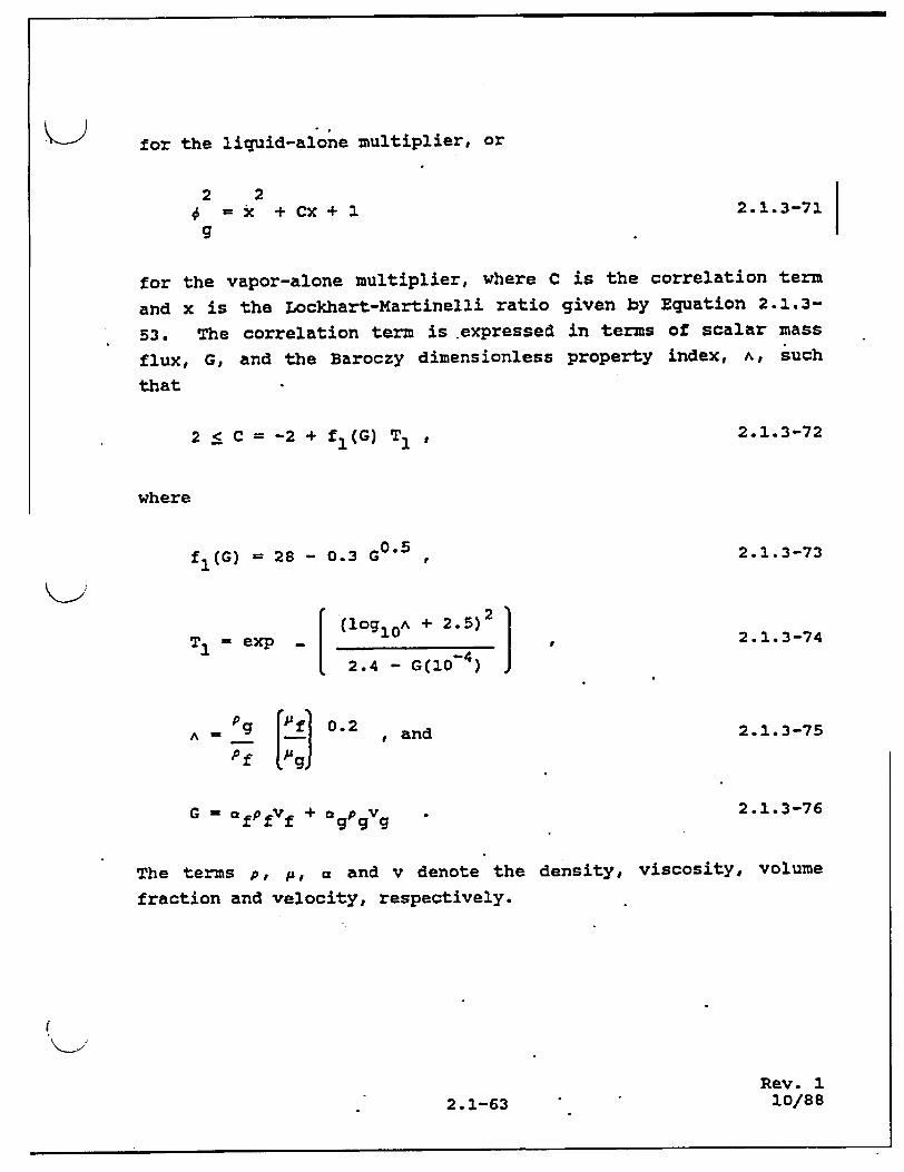
for the liquid-alone multiplier, or

2 2 S=x +Cx+I

g

2.1.3-71

for the vapor-alone multiplier, where C is the correlation term

and x is the Lockhart-Martinelli ratio given by Equation 2.1.3

53. The correlation term is expressed in terms of scalar mass

flux, G, and the Baroczy dimensionless property index, A, such

that

2 • C = -2 + f3(G) T1 , 2.1.3-72

where

fl(G) - 28 - 0.3 G0 . 5 2.1.3-73

T -. exp -( ( 1 go 0 + 2.5) 2

2.4 - G(10 -4 )

P [9 ) 0.2, and

2.1.3-74

2.1.3-75

G - afPfvf + a gp gVg 2.1.3-76

The terms p, u, c and v denote the density, viscosity, volume

fraction and velocity, respectively.

I.

Rev. 1 10/88

2.1-63

If the H.T.F.S. correlation is combined with the wall friction formulations by combining. Equations 2.1.3-45 through 2.1.3-48, 2.1.3-51 through 2.1.3-53, 2.1.3-70, and 2.1.3-71, then

2•f ag g

I A Pfcav(f v 2 + C Pf• Cv•f) 2 A;g ccreg) 2 0.5 2D

+ A1Pg(agvg)g 2 2.1.3-77

This equation can then be combined with Equation 2.1.3-68 and 2.1.3-69 and simplified such that

FWF(a•f) = 0w 2D (AP f(afvf)

2D +C(Aip f (C fVf)2A Pgcg) 2) 0.5

g gg g~ cgQ~gPgVg + -fwifPfvf

2.1.3-78

for the liquid, and

FW~~p)-~ Pg~giVgI 2

FWG(ap - Crg ( 2D 0 2

2} " 2D "p (Clvf

" APgP(CzgVg) 2 A g + a v 9 W• g9 9~ f fw~f fv

2.1.3-79

for the vapor.

2.1-64

In RELAP5 the friction factor and velocity terms are calculated in such a manner that as the velocity terms disappear the equations give the correct limits. For example, the friction factor terms are evaluated such that

6 4 pf

Dp f

livfn I o fvf cf VfI1 ..O

lim, (Ag9 (Y2jg vg)1

I agj g-

and the velocity terms are evaluated such that

u n lira fI As C M II n v g9 1 vfI1 -#0 jvg~ 1.00

2.1.3-81

Hence, for stagnant flow or single-phase conditions, a positive and finite friction coefficient is always calculated. Thus, the numerical possibility of an infinite or negative friction coefficient is eliminated.

In Equations 2.1.3-78 and 2.1.3-79, flow regime effects are included in the terms (afw/af) and (agw/ag) for the liquid and

vapor, respectively. These terms are such that

acfw = I a w 2.1.3-82

and

2.1.3-83f I - g .

2.1-65

im I Of vf

64p =

DPg

2.1.3-80

S.... ... m NM

\

lia c•. 1 '0 g i 9

Equations 2.1.3-80 and 2.1.3-83 are restricted such that as overall phasic volume fraction disappears its corresponding wall film volume fraction disappears so that

11ra [afW1 =I and 3,ia w = 1 , 2.1.3-84

f (f

and similarly,

-rn al and lim f i . 2.1.3-85 a-+0 a a-0 j

Flow Regime Factors for Phasic Wall Friction

Phasic wall friction is expressed in terms of wall shear stress, which in turn requires knowledge of the surface area wetted by each phase. From the flow regime model discussed in section 2.1.3.1, expressions for the wall -film phasic volume fractions can be derived. Using these expressions, the phasic 'wall friction factors that appear in Equations 2.1.3-56 and 2.1.3-57 may then be completed.

In the flow regime map, seven flow regimes are modeled, which are: for pre-CHF heat transfer, the bubbly, slug, and annular mist; for post-CHF heat transfer, the inverted-annular, invertedslug and mist; and for stratified flow, the vertically and horizontally stratified. For the transition regime between preand post-CHF heat transfer, an interpolation scheme is also implemented in the code.

To implement flow regime effects in the two-phase wall friction model, first consider the wall liquid and vapor volume fractions.

2.1-66

4

K> These terms are

Pf p=afw p

2.1".3-86

which represents the liquid volume fraction in the wall film, and

Pg gw• 2.1.3-87

which represents the vapor volume fraction in the wall film where

the terms pf, pg, and p are the perimeters wetted by the liquid,

vapor, and mixture, respectively. Then, from the flow regime

model these are formulated for all "of the flow regimes as

follows:

For the bubbly regime

Sfw = of and agw = ag 2.1.3-88

where of, ag are the overall liquid and vapor volume

fraction, respectively.

For the slug regime

fw 1-ags and agw ogs 2.1.3-89

where ags is given by Equation 2.1.3-29.

For the annular-mist regime

1

4 afw = (Off) 4and 0gw

1

-1 f f ) 4 2.1.3-90

where aff is given by Equation 2.1.3-34.

2.1-67

For the inverted-annular regime

4 1 •g (agg) 4 and af = 1.- (Ctgg) 4 , .. 39

9 an 9 2.1.3-91

where agg is the inverted form of Equation 2.1.3-34.

For the inverted-slug regime

a fw " fs anda I afs, 2.1.3-92

where as is the inverted form of Equation 2.1.3-29.

For the mist regime

afw , af and cc a 2.1.3-93

which is similar to the bubbly regime.

For the vertically stratified regime

Sfw =f andf a =ag . 2.1.3-94

For the horizontally stratified regime

e 9- 1- -- and a - - 2.1.3-95

fw i gw i

where 9 results from the solution of Equations 2.1.3-17 and

2.1.3-18.

2.1-68

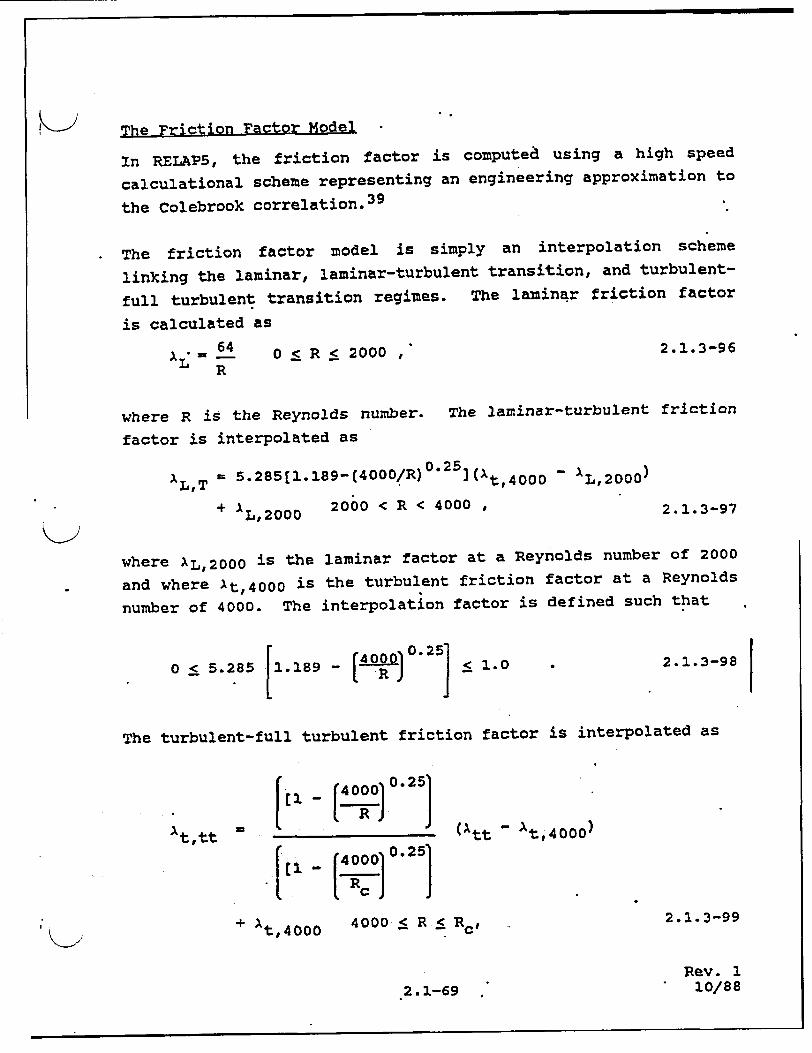
ý1ý

64 R

0 < R < 2000 ,

where R is the Reynolds number.

factor is interpolated as

2.1.3-96

The laminar-turbulent friction

5L,T 5.28511 189-(4000/R) 0 .25] I 4000 L, (t,00

+ AL,2000

- XL, 2000)

2000 < R < 4000 , 2.1.3-97

where AL,2000 is the laminar factor at a Reynolds number of 2000

and where At,4000 is the turbulent friction factor at a Reynolds

number of 4000. The interpolation factor is defined such that

0 < 5.285 1.189 - < 1.0 [1.189R - j0].52.1.3-98

The turbulent-full turbulent friction factor is interpolated as

(At'tt =

Cl~400002)

(\tt - At, 4 0 0 0 )

El ( f4000] 0.25)

+ At, 4 0 0 04000 < R < Rc, 2.1.3-99

Rev. 1 10/882.1-69

-I

The Friction Factor Model

In RELAP5, the friction factor is computed using a high speed

calculational scheme representing an engineering approximation to

the Colebrook correlation.3 9

The friction factor model is simply an interpolation scheme

linking the laminar, laminar-turbulent transition, and turbulent

full turbulent transition regimes. The laninar friction factor

is calculated as

where the interpolation factor is defined such that

[LOOO)0.25] 0

RC-0001 0.25]

2.1.3-100

and R6 is the critical Reynolds number at which the Colebrook equation gives a constant friction factor of

Att [1.74 - 2LOgl 0(2c/D)] 22.1.3-101

and where e is the surface roughness.

The critical Reynolds number is given as

Rc M378.3

S 0.5 B-tt

2.1.3-102 ý,_

where 2c/D Z 10-9.

"If precise values for At,4 0 00 are used, Equations 2.1.3-96 and 2.1.3-97 are identical to the formulations used in the Colebrook friction factor model for the laminar and transition regimes. Equation 2.1.3-101 is also identical to the solution of the Colebrook model for Reynolds numbers greater than the critical Reynolds number. Therefore, the interpolation scheme in the friction factor model lies in the formulation of Equation 2.1.399, which is linear in (l/R) 0 -2 5 . The maximum deviation between the friction factor calculated using Equation 2.1.3-99 and that calculated using the Colebrook correlation is within the third significant figure for a moderate c/D of 0.0003, and as e/D increases the deviation decreases until at an c/D such that Rc < Sk<2

2.1-70

P

4000 the value given by Equation 2.1.3-99 is precisely that of

Equation 2.1.3-101. In any case, the results calculated using

Equation 2.1.3-99 are negligibly different from those calculated

by the Colebrook equation. This accuracy is achieved using a

good estimate for At,4000 given by

At, 4 0 0 0 = 0 + (•tt -.i) 2.1.3-103

where %o is a constant evaluated from the Blasius smooth pipe

formula at a Reynolds number of 4000, such that

A0 = 0.0398. 2.1.3-104

The coefficients have been evaluated as

K - 0.558 and A1 = 0.0158 2.1.3-105

by the method of least sguares.

In calculational schemes, it is desirable to evaluate the

friction factor in terms of AlIvi so that the limiting terms will

be correctly calculated as defined by Equations 2.1.3-80. For

this case, the Reynolds number must be defined as

= _PD lv I~v I

and Equation 2.1.3-97 can be rewritten as

2.1.3-106

AL + L[5.285(l.189 - R )J(L[(l - R*)/(l - R*)]

(Att - At, 4 000) IOvI +At, 4 0 0 0I1'vI - AL) 2.1.3-107

Rev. 1 10/882.1-71

K>

(

where L(y) denotes a general limit function.such that

R* = (4000/R).25 and

R k 2000

R = (4000R) 2 5 , and c ' .

and Rc Z 4000 ,

2.1.3-108

2.1.3-109

2.1.3-110

and where the laminar term is

* 64p L pD 2.1.3-111

The accuracy of the improved friction factor model can be observed in Figure 2.1.3-4, which is a plot of results calculated

by -Equation 2.1.3-107 compared to similar results calculated by the Colebrook equation. Four curves are plotted for each model

representing roughness to diameter ratios of 2e/D - 0.0, 0.0006,t 1 0.02, and 0.1, respectively. Equation 2.1.3-107 results are plotted and labeled as INTERP in the plot legend. Colebrook equation results are plotted and labeled as COLBRK in the plot

legend. The axes of the plot are scaled logarithmically.

2.1-72

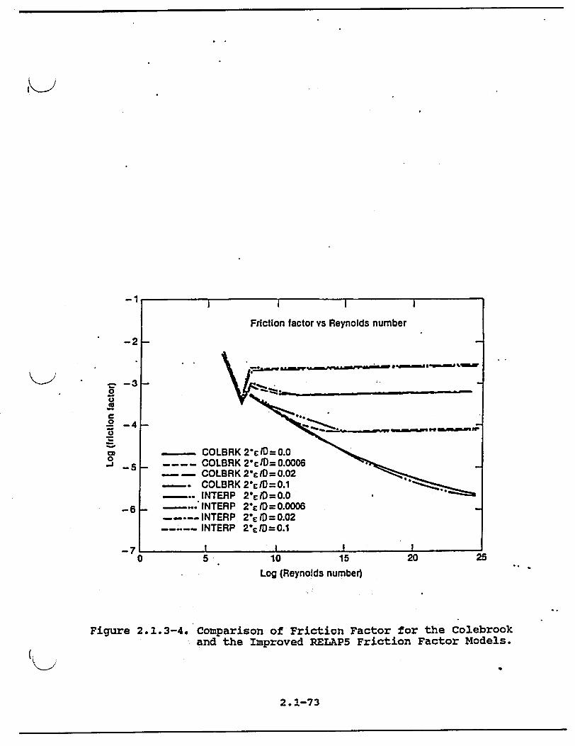
-1

0 4. €0

C 0

0 -J

-3

-4

-5

-6

-70 5 10 15 20 25

Log (Reynolds number

Figure 2.1.3-4. Comparison of Friction Factor for the Colebrook and the Improved RELAP5 Friction Factor Models.

2.1-73

Friction factor vs Reynolds number

-_____________ I - I - %

COLBRK 2"cD=0.0 COLBRK 2*cID=0.0006

--- COLBRK 2 "c/D=0.02 - - COLBRK 2*c/D=0.1

-- ,, INTERP 2*° /D = 0.0 _ -.-- ,,"INTERP 2"*c )= 0.0006

-.--. INTERP 2"€/D=0.02 INTERP 2"c/D=0.1

-2

2.1.3.4. Inter~hase Heat and Mass Transfer

The interface mass transfer is modeled according to the

thermodynamic process, interphase heat transfer regime, and flow

regime. After the thermodynamic process is decided, the flow

regime map discussed in section 2.1..3.1 is used to determine .the

"phasic interfacial area and to select the interphase heat

transfer correlation.

The mass transfer model is formulated so that the net interfacial

mass transfer rate is composed of two components which are the

mass transfer rate at the wall and the mass transfer rate in the

bulk fluid, which is expressed as

F r w + rig 2.1.3-112

For system components in which wall heat transfer is modeled,

mass transfer at the wall is calculated according to the wall

heat transfer model and mass transfer to the bulk fluid is \.

calculated according to the interphase heat transfer regime and

flow regime. For system components in which wall heat transfer

is not modeled, mass transfer at the wall is ignored and mass

transfer in the bulk fluid is modeled according to the interphase

heat transfer regime and flow regime.

For components modeling wall heat transfer processes, the

interfacial mass transfer at the wall is calculated from the

total wall-to-liquid heat transfer minus the wall-to-liquid

convective heat transfer. For these processes, the heat transfer

model developed by Chen, as discussed in section 2.2.2.1, is used

to model the total wall to liquid heat transfer. The Chen model

assumes that the total wall-to-liquid heat transfer is composed

of boiling and convective heat transfer and that the interfacial

mass transfer at the wall is mainly due to boiling heat transfer.

Consequently, the contribution, due to convective heat transfer

must be subtracted from the total wall to liquid heat transfer in,

2.1-74

.> order to calculate the interfacial mass transfer at the wall. Correlations used to calculate interfacial mass transfer at the

wall for different heat transfer regimes are discussed in section

2.2.2.

For components not modeling wall -heat transfer and for the

general bulk mass transfer processes, the interfacial mass

transfer in the bulk fluid is modeled according to the flow

regime. In the bubbly flow regime, for the liquid side,

interfacial mass transfer is the larger of either the model for

bubble growth developed by Plesset and Zwick 4 7 or the model for

convective heat transfer for a spherical bubble, 4 8 and for the

vapor side, an interphase heat transfer coefficient is assumed

that is high enough to drive the vapor temperature toward

saturation. Analogously, in the annular mist regime, for the

vapor side, a convective heat transfer model for a spherical

droplet is used for the interphase heat transfer coefficient, and

for the liquid side, an interphase heat transfer coefficient is

assumed that is high enough to drive the liquid temperature

toward saturation. correlations used to calculate interfacial

mass transfer in the bulk fluid are summarized in Table 2.1.3-1.

For condensation processes, the interfacial mass transfer in the

bulk fluid, for the liquid side, is calculated by the Unal bubble

collapse model 4 9 in the bubbly flow regime and by the Theofanous

interfacial condensation model 5 1 in the annular mist flow regime

and for the vapor side, a large interphase heat transfer

coefficient is assumed in order to drive the vapor temperature

toward saturation.

2 . 1-75

Table 2.1.3-1. RELAP/MOD2 Interfacial Mass Transfer in Bulk

Fluid.

Deoressurization Process (Tf > Tsat)

1. Bubbly Flow Regimes:

Qif Hif (Ts - Tf).,

where

12 ATsat Pf(C) k (Plesset-Zwick) 4 7 (w/m 3 -K)

rdb2 Pghfg

Hif = MAX

6Kf 0.5 0.333 (2 + 0.74 Reb Prf ) (Force convection

b2 for single bubble),,

4 2

Reb = Pf vg vfl (Bubble Reynolds number), •f

db = bubble diameter (m),

Qig = ig (Ts -T ), and

where

ig 2 kg NUib and db2

Nuib =10

2. Annular-Mist Regime:

Qif = Hif (Ts - Tf),

2.1-76

Table 2.1.3-1. (Continued)

where

6 (1-ct ) Hif = kf NUid,

Nuid = 10 , and

Qig = Rig (Ts -T),

where

H 6(lg) (2. + 0.74 R 0 5 g0 3 3

ig g g ed pr

ddo.8 kg (Pg) o.

+ 0.0023 (Re)g 0 kg 2

9 2 De

Red = P g dd lvg__ (Droplet Reynolds number), and

P9g

dd = drop diameter (m).

Heat Transfer Process (T _< T f sat

1. Bubbly Flow Regime:

Oif = Hif (Ts - Tf)

2.1-77

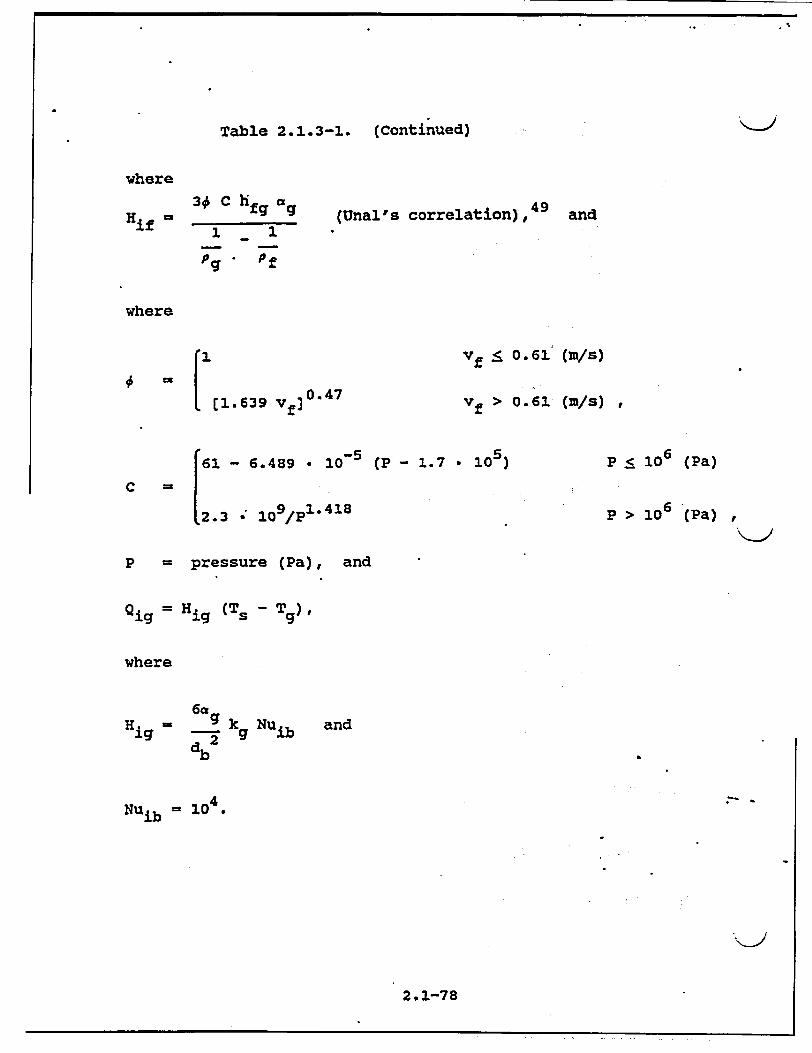
Table 2.1.3-1. (Continued)

where 3ý C hfg 9g

Hif 1

p.

(Unal's correlation),49 and

where

[1.639 Vf0.47

Vf ;S 0. 61 (m/s)

Vf > 0.61 (m/s)

[613- 6.489 10-5 (P - 1.7

12.3 - 109 /pi. 4 1 8

105) P < 106 (Pa)

P > 106 (Pa)

P = pressure (Pa), and

Qig = Hig (Ts - T),

where

6 a g 9 k u ig 2 g N

g b

and

Nuib - 10

2.1-78

C

'1-1ý

Table 2.1.3-1. (Continued)

2. Annular-Mist Flow Regime:

Similar to the depressurization process.

Condensation Process

1. Bubbly Flow Regime:

similar to the heat transfer process.

2. Annular-Mist Flow Regime:

Qif = Hif (Ts - Tf),

where

8. (Ts - Tf) /d2

Hif = 6 [2. + S ( kf (1-a )/d

Tm - Tf

+ 0 Pf * vf Cpf Afilm,

Afilm = area of film per unit volume, and

Ts - Tf Tm =

1 + CPg(T - Ts)/hfg

The first term on the right side uses the condensation of aT'

single droplet in superheated steam model developed by Brown. 5 0

2.1-79

Table 2.1.3-1. (Continued)

The second term on the right side uses the film condensation

model developed by Theofanous. 5 1

Qig - Hig (Ts - Tf)

where

H 6 (l-a)k NU and

iigd

dd2

NUid 105.

2.1-80

2,1,3.5. Horizontal Stratification Entrainment Model

Under stratified conditions in horizontal components, the void

fraction of flow through a junction may be different from the

upstream volume void fraction. Consequently, the regular

donoring -scheme for junction void fraction is no longer ap

propriate because vapor may be pulled through the junction and

liquid may also be entrained and pulled through the junction.

The correlations describing the onset of vapor pull through and

liquid entrainment for various geometrical conditions were

summarized by Zuber. 7 3

The incipient liquid entrainment is determined by the

that

Vg9 ŽVge

where Vge is given by the expressions

geg v 5.7 [-]32BY

PEPg/

Vge Id r-1 / B(pp)(-)]'

for an upwardly oriented junction7 3 , and

Vge ' 3.25 (D/2 _I 32 B (pfpg) (D/2-11)f'

2

d ~ Pg

criterion

2.1.3-113

2.1.3-114

2.1.3-115

for a centrally oriented Junction, 7 4 , 7 5 where d is the junction

diameter and 11 is the liquid level.

The condition for the onset of vapor pull-through- is determined

by the criterion

vf > vfp 2.1.3-116

2.1-81

/

where

(1 Dc/2f / 2 (B (p~ - Pgd} / Vfp 3.25 , 2.1.3-117

fp d Pf

and where

'i for a centrally located or side junction

0o for downward oriented junction. 7 6 , 7 7

Equations 2.1.3-113 through 2.1.3-117 together with the horizontal stratification criterion (Equation 2.1.3-15) from section 2.1.3.1, form the basis for calculating the junction void fraction under stratification conditions.

For liquid entrainment, the junction liquid fraction, fj, ir related to the donor volume liquid fraction, afK, by theK-) expression

a f,j = a f,k [i - exp (-ClVg/Vge - lOv2 v) 2.1.3-118

where VgL is from Equation 2.1.3-16. For vapor pull-through, the

junction void fraction, ag,j, is given by the expression

cgj agjk (1 - exp 2Vf/Vfp - v 2Ov 2VL) 2.1.3-119

The constants C1 and C2 for Equations 2.1.3-118 and 2.1.3-119 are obtained by comparisons of code calculations with experimental

data.78-80

2.1-82

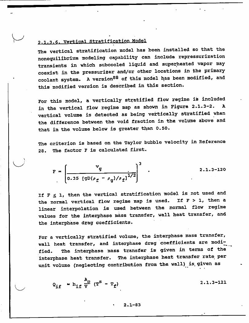
2.1.3.6. Vertical Stratification Model

The vertical stratification model has been installed so that the

nonequilibrium modeling capability can include repressurization

transients in which subcooled liquid and superheated vapor may

coexist in the pressurizer and/or other locations in the primary

coolant system. A version8 8 of this model has been modified, and

this modified version is described in this section.

For this model, a vertically stratified flow regime is included

in the vertical flow regime map as shown in Figure 2.1.3-2. A

vertical volume is detected as being vertically stratified when

the difference between the void fraction in the volume above and

that in the volume below is greater than 0.50.

The criterion is based on the Taylor bubble velocity in Reference

28. The factor F is calculated first.

F 1g. 2.1.3-120 0.35 [gD(pf - p 9)/Pfl 1/2

If F < 1, then the vertical stratification model is not used and

the normal vertical flow regime map is used. If F > 1, then a

linear interpolation is used between the normal flow regime

values for the interphase mass transfer, wall heat transfer, and

the interphase drag coefficients.

For a vertically stratified volume, the interphase mass transfer,

wall heat transfer, and interphase drag coefficients are modi

fied. The interphase mass transfer is given in terms of the

interphase heat transfer. The interphase heat transfer rate per

unit volume (neglecting contribution from the wall) is. given as

Ac h A Ts-cf 2.1.3-121 S j ~Qif = if V-(T-Tf

2.1-83

and

A 0 5 Qig =h'g (T -Tg), 2.1.3-122

where hjf and hi are the liquid side and vapor side interface heat transfer coefficients, Ae is the cross-sectional flow area (equal to the interfacial area when stratified), and V is the volume. A value of 10 w/m 2-K is used for both hif and hig in the vertical stratification model. The wall heat transfer coefficients hwf and h., are partitioned with respect to their corresponding vapor and liquid fractions (af and a when vertical stratification occurs. For the junction above the vertically stratified volume, an interphase drag coefficient of 10-I N-s 2/m 5 is used.

There is no specific edit information output for a vertically stratified volume.

2.1.3.7. Water Packing Mitigatfon Scheme

Large pressure spikes that cannot be explained by known physical "phenomena are at times encountered when Eulerian type codes are used to analyze integral systems tests or reactor accidents. These spikes usually do not affect overall transient behavior, but in some cases may affect important localized behavior (e.g. delivery of coolant to the reactor core). A water packing scheme has been installed to mitigate these spikes.

The water packing scheme closely follows the method used in the TRAC code. 8 9 , 9 0 It involves a detection scheme to determine whefii

a pressure change occurs in a volume containing mostly liquid. It then imposes changes to the momentum equations, followed by a recalculation of the pressure solution using the "sparse matrix solver.

2.1-84

The detection logic used in the water packing scheme evolved from

experience gained in running a vertical fill problem. 9 1 The

scheme requires a pressure increase of 0.23% or more, a void

fraction (ag) less than or equal to 0.12, the liquid temperature

(Tf) to be less than the saturation temperature (Ts), the volume

to be flagged as vertically stratified, and the volume above to

be highly voided. Thus a legitimate water hammer would not be

detected in the water packing scheme.

The next part of the scheme involves altering the momentum

equations so that only small pressure changes will occur in the

volume that fills with water. The scheme involves modifying the

coefficient that multiplies the pressure change in the filling

volume'. The modification multiplies this coefficient by 106.

This is discussed in more detail in the next paragraph. Since

the pressure solution is rejected when water packing occurs, the

pressure calculation is repeated using the sparse matrix solver.

The finite difference form of the phasic momentum equations used

can be written

vn+l = vnexp _ (VFDP) ((n+l _ P n - (P +I - P] f,) f P )j)

2.1.3-123

and

vn+1 nexp _ (VGDP)n (7 - l+K - Pn))

2.1.3-124

where vnexp and vn'exp contain all the old time terms and nf,j ngtj

(VFDP) iand (VGDP) contain all the terms that- multiply. the

pressure change. Consider the filling example in .Figurle.2.1.3-5

where volume K is full of liquid and volume L is full of steam.

The change to the momentum equations is to multiply the (Pn 1

) terms by106, wn+l to be approximately the PK trm by 10,which forces YK

2.1-85

same asP . Thus, the water filled K volume will not show a pressure spike. The momentum equations then have the form

vn+ vnexp - (VFDP)n(pn+1 fj f- i vj • L - P + (VFDP)n ( 10) 6 .1. n

2.1.3-125

n- G cpn+l - '1 + nVGDPIn0 6 n 6 n+1 n +Ig,j vg,j (,V ' L E +VGDP) (K PX)

2. 1. 3-126

In addition to the modification of the momentum equation, the interphase drag is reduced to 10-1 (N - s 2 )/m 5 for junction j.

/M nction J

2.1-86

and

Volume L

T_ _ T Junction

Volume K PK

Figure 2.1.3-5. Two Vertical Vapor/Liquid Volumes.

2.1-87

2.1.4. Sipecial Process Models

Certain models in RELAPS/MOD2 have been developed to simulate special processes. These models, described in the following subsections, include: choked flow, abrupt area change, crossflow junction, and branch models.

2.1.4.1. Choked Flow Models

Two mutually exclusive models are available for calculating choked flow in RELAPS/MOD2. The first option uses the original built-in Ransom-Trapp method. The second option uses a table interpolation with any of the four following critical mass flux tables: Extended Henry-Fauske, Moody, HEM, or Murdock-Bauman.

Ransom-Trapp Choked Model

A choked flow model developed by Ransom and Trapp6 2 ' 1 8 is included in RELAP5 primarily for calculation of the mass discharge from the system at a pipe break or a nozzle. Generally, the flow at the break or nozzle is choked until the system pressure nears the containment pressure. The choked flow model is used to predict if the flow is choked at the break or nozzle and, if it is, to establish the discharge boundary condition. In addition, the choked flow model can be used to predict existence of and calculate choked flow at internal points in the system.

Choking is defined as the condition wherein the mass flow rate becomes independent of the downstream conditions (that point at which further reduction in the downstream pressure does not change the mass flow rate). The fundamental reason that choking-.. occurs is that acoustic signals can no longer propagate upstream. This occurs when the fluid velocity equals or exceeds- the propagation velocity. The choked flow model is based on a definition that is established by a characteristic analysis using time-dependent differential equations.

2.1-88

Consider a system of n first-order quasi-linear, partial

differential equations of the form

A(U) (aU/Ot) + B(U) (8U/8x) + C(U) 0 . 2.1.4-1

The characteristic directions (or characterization velocities) of

the system are defined6 3 ' 6 4 as the roots, Ai(i _ n), of the

characteristic polynomial

(A - B) = 0 • 2.1.4-2

The real part of any root, Ai, give the velocity of signal

propagation along the corresponding characteristic path in the

space/time plane. An imaginary part of any complex root, xi,

gives the rate of growth or decay of the signal propagating along

the respective path. For a hyperbolic system in which all the

roots of Equation 2.1.4-2 are real and nonzero, the number of

boundary conditions required at any boundary point equals the

number of characteristic lines entering the solution region as

time increases. If we consider the system (Equation 2.1.4-1) for

a particular region 0 _< x < L, and examine the boundary

conditions at x = L, as long as any Ai is less than zero, we must

supply some boundary information to obtain the solution. If Ai

is greater than or equal to zero, no boundary conditions are

needed at x - L, and the interior solution is unaffected by

conditions beyond this boundary.

A choked condition exists when no information can propagate into

the solution region from the exterior. Such a condition exists

at the boundary point, x = L, when

Aj k 0 for all J < n . 2.1.4-3

These are the mathematical conditions satisfied by the equations

of motion for a flowing fluid when reduction in downstream

2.1-89

pressure ceases to result in increased flow rate. It is well

"known65 that the choked condition for single-phase flow occurs

when -the fluid velocity just equals the local sound speed. For this case, one of the Aj's is Just equal to zero. For the twophase case, it is possible for all Aj's to be greater than zero under special conditions whichcan exist during discharge of a subcooled liquid.

During the course of the RELAP5 development, extensive investigation was carried out to determine two-phase choked flow criterion under two assumed conditions:a (a) thermal equilibrium between phases, and (b) adiabatic phases without phase change (frozen). 6 6 The frozen assumption was in poor agreement with data, compared to the thermal equilibrium assumption. Therefore, the thermal equilibrium assumption with slip is used as the basis for the RELAP5 choked flow criterion. In the following paragraphs, theoretical aspects of choked flow are discussed.

Ransom-Trapp Model Choking Criterion for Nonhomogeneous, Equilibrium Two-Phase Flow

The two-fluid model for the conditions of thermal equilibrium (equilibrium interphase mass transfer) is described by the overall mass continuity equation, two phasic momentum equations, and the mixture entropy equation. This system of equations is

a9 apg 9+ afpf)/at + (aPgpgvg + afpfVf)/ax 0 2.1.4-4

SgPg avg/at + vg(avg/ax)] + ag(aP/ax)

+ CagafP(Bvg/Bt - av /8t) m 0, 2.1.4-5.

aThe hydrodynamic model is not based on either *of these assumptions; however, the purpose of this analysis is simply to establish a criterion for choked flow and thus, there is no conflict with the basic hydrodynamic model. I

2.1-90

Ofpf[Rvf/at + v:C(avf/ax)] + af(OP/ax)

+ CafgP(Ovf/at - aVg/at) = 0 2.1.4-6

and

a(agPgSg + lfpfSf)/at + 8(agpgSg g + GfPfSfvf)/aX - 0

2.1.4-7

The momentum equations include the interphase force terms due to

relative acceleration. 1 6 These force terms have a significant

effect on wave propagation velocity and consequently on the

choked flow velocity. The particular form chosen is frame

invariant and, symmetrical, and the coefficient of virtual mass,

Cagafp, is chosen to ensure a smooth transition between pure

vapor and pure liquid. For a dispersed flow, the constant, C,

has a theoretical value of 0.5, whereas for a separated flow, the

value may approach zero. The energy equation is written in terms

of mixture entropy, which is .constant for adiabatic flow (the

energy dissipation associated with interphase mass transfer and

relative phase acceleration is neglected).

The nondifferential source terms, C(U), in Equation 2.1.4-1 do

not enter into the characteristic analysis or affect the

propagation velocities. For this reason, the source terms

associated with wall friction, interphase drag, and heat transfer

are omitted for brevity in Equations 2.1.4-4 through 2.1.4-7.

In the thermal equilibrium case, pg, pf, Sg, and Sf are known

functions of the pressure only (the vapor and liquid values alon•"*

the saturation curve). The derivatives of these variables are

designated by an asterisk as follows

p dpS/dP and p * dp 2.1.4-8 f f 9.

2.1-91

and

Sf dS dP andS d'. e 2.1.4-9

The system of governing equations (Equations 2.1.4-4 through 2.1.4-7) can be written in terms of the four dependent variables, ag, P, Vg, and vf, by application of the chain rule and the

property derivatives (Equations 2.1.4-8 and 2.1.4-9). Thus, the system of equations can be written in the form of Equation 2.1.4

1 where the A and B are fourth-order square coefficient matrices.

The characteristic polynomial that results is fourth-order in A and factorization can only be carried out approximately to obtain

the roots for A, and establish the choking criterion. The first two roots are

{afpg + pc/2 ± (pc/2)2_- agczfpgpf] /2 vg

=+ {k 9Pf + PC/2 + pC/22 a- amfP g-0f] } f~ A1 , 2 (ccfPg + pc/2) + (a gpf + pC/2)

2.1.4-10

These two roots are obtained by neglecting the fourth-order factors relative to the second-order factors in (X - vg) and (A - vf). There are no first- or third-order factors. Inspection of Equation 2.1.4-10 shows that A1 ,2 have values between Vg and vf; thus, the fourth-order factors (A - Vg) and (A - vf) are small (i.e., neglecting these terms is

justified). The values for A1 , 2 may be real or complex depending on the sign of the quantity [(pC/2) 2 - OgafPgPf].

2.1-92

'K-

where

V = (ag9P Vg + afPf f)/P , 2.1.4-12

a=aHe[CP2 + P(agpf + afPg)]/(CP2 + Pgpf)}i/2 if2.1.4-13

and

[ -9Pf - OfP9) , pP• P f - CrPc) D 0.5 (PC + afPg + a gPf) + (Pg Pf + cp2)

P P(aer~ __ _2_ __ _ _2 _

HE pgpf (Sg9 - S

The quantity, aH, is the homogeneous equilibrium speed

The roots, A3 ,4, have only real values.

2.1.4-14

of sound.

The general nature and significance of these roots is revealed b•'

applying the characteristic considerations. The speed of

propagation of small disturbances is related to the values of the

characteristic roots. In general, the velocity f -propagation

corresponds to the real part of a root and the growth or

attenuation is associated with the complex part of the root.

2.1-93

The remaining two roots are obtained by dividing out the

quadratic factor containing A1 1 , 2 , neglecting the remainder, and

subsequent factorization of the remaining quadratic terms. [This

procedure can be shown to be analogous to neglecting the second

and higher-order terms in the relative velocity, (Vg - vf). ] The

remaining roots are

A3 , 4 ' v + D(vg - vf) ± a 2.1.4-11

K)_

Choking will occur when the signal, which propagates with the largest velocity relative to the fluid, is just stationary, that is,

AR 0 for j S 4 2.1.4-15

and

A R _> 0 for all i yA j. 2.1.4-16'

The existence of complex roots for A1 , 2 makes the initial boundary value problem ill-posed. This problem has been discussed by many investigatorsl 3 , 2 0 and the addition of any small, second-order viscous effects renders the problem wellposed. 13,21 The whole phenomenon of systems with mixed orders of derivatives and A first-order system with the addition of a small, second-order term, has been discussed and analyzed by Whitham. 6 4 He has shown that the second-order viscous terms giv\,> infinite characteristic velocities. However, very little information is propagated along these characteristic lines and the bulk of the information is propagated along characteristic lines defined by the first-order system. We conclude that the ill-posed nature of Equations 2.1.4-4 through 2.1.4-7 can be removed by the addition of small, second-order viscous terms that have little effect upon the propagation of information. Therefore, the choking criterion for the two-phase flow system analyzed here is established from Equation 2.1.4-15.

The explicit character of the choking criterion for the two-phase flow model defined by Equations 2.1.4-4 through 2..1.4-7 ia.. examined. Since the two roots, A 1 , 2 , are between the phase velocities, vf and Vg, the choking criterion is eitablished*.from the roots, A3 , 4 , and Equation 2.1.4-15. The choking criterion is

v Dv - = ±a. 2.1.4-17

2.1-94

The choking criterion can be rewritten in terms of the mass mean

and relative Mach numbers

MV = v/a and Mr - (Vg - vf)/a 2.1.4-18

as

Mv + DMr = 1. 2.1.4-19

This relation is similar to the choking criterion for single

phase flow where only the mass average Mach number appears and

choking corresponds to a Mach number of unity.

The choking criterion (Equation 2.1.4-19) is a function of the

two parameters, D and a. In Figure 2.1.4-1, a is plotted as a

function of the void fraction, ag, for a typical steam/water

system at 7.5 MPa with C equal to zero (the stratified

equilibrium sound speed), C equal to 0.5 (the typical value for a

dispersed flow model), and in the limiting case when C become

infinite (homogeneous equilibrium sound speed). From Figure

2.1.4-1 it is evident that the virtual mass coefficient has a

600 r- i II

1

0 W,

400

200

0 0.2 0.4 0.6 0.1 Vapor fraction

Figure 2.1.4-1. Equilibrium Speed of Sound as a Function of Void Fraction and Virtual Mass Coefficient.

2.1-95

significant effect upon the choked two-phase flow dynamics. 1 4

To establish the actual choked flow rate for two-phase flow with

slip, the relative velocity term in Equation 2.1.4-19 must also

be considered. The relative Mach number coefficient, D, is shown

in Figure 2.1.4-2 for values of C equal to 0, 0.5, and •. It is

evident from these results that the choked flow velocity can

differ appreciably from the mass mean velocity when slip occurs.

It is significant that the variation of the choked flow criterion

from the homogeneous result is entirely due to velocity

nonequilibrium, since these results have been obtained under the

assumption of thermal equilibrium. The particular values of

0.6

0.3

0

"-0.3

-0.60 0.8

Vapor fraction

Figure 2.1.4-2. Coefficient of Relative Mach Number for Thermal Equilibrium Flow as a Function of Void Fraction and Virtual Mass Coefficient.

2.1-96

0

ca 2

K>

these parameters used in the model are discussed later in this

section.

gansom-TraDp Subcooled Chokina Criterion

The previous analysis assumes two-phase conditions exist

throughout the break flow process. However, initially and in the

early phase of blowdown, the flow approaching the break or break

nozzle will be subcooled liquid. Under most conditions of

interest in LWR systems, the fluid undergoes a phase change at

the break. The transition from single- to two-phase flow is

accompanied by a discontinuous change in the fluid bulk modulus.

This is especially true for the liquid-to-liquid/vapor

transition. For example, at 600 KPa, the ratio of the single- to

two-phase sound speed at the liquid boundary is 339.4. Thus,

considerable care must be exercised when analyzing a flow having

transitions to or from a pure phase (a discontinuity is also

present at the vapor boundary, but the ratio is only 1.069).

To understand the physical process that occurs for subcooled

upstream conditions, consider the flow through a

converging/diverging nozzle connected to an upstream plenum with

subcooled water at a high pressure. For a downstream pressure

only slightly lower than the upstream pressure, subcooled liquid

flow will exist throughout the nozzle. Under these conditions

the flow can be analyzed using Bernoulli's equation, which

predicts a minimum pressure, Pt, at the throat.a As the

downstream pressure is lowered further, a point is reached where

the throat pressure equals the local saturation pressure, Psat.

If the downstream pressure is lowered further, vaporization will

take place at the throat.b When this happens, the fluid sounaT''

aFor all practical cases of choking, the subcoolea water can be considered incompressible with infinite sound speed.

bAn idealized one-dimensional homogeneous equilibrium model is

assumed in the example.

2.1-97

speed lowers drastically, but continuity considerations dictate\•-• that the velocity, vt, of the two-phase mixture (at the point of minuscule void graction) just equals the velocity of the subcooled water slightly upstream of the throat. When this occurs, vt in the subcooled region is less than the water sound speed, but in the two-phase region, vt can be greater than the two-phase sound speed. Hence, the subcooled water has a Mach number (M) less than one, whereas the two-phase mixture at the throat has a Mach number greater than one. Under these conditions (Mach numbers greater than one in the two-phase region), downstream pressure effects are not propagated upstream and the flow is choked. In particular, the supersonic two-phase fluid at the throat must increase in velocity and the pressure drop as it expands in the diverging sectiona (transition back to

(a)

up (a)

Pup(b) Pup(c)

Psat

(b) (C)

K�)

"vt p(a) sat] Vt = (b)Psat] aHE vt = aH-E Pup(c)Psatj 12 p 2 fp

Figure 2.1.4-3. Subcooled Choking Process.

aIn a supersonic flow, a diverging nozzle implies an increase in velocity.

2.1-98

M-eI M>1 M>I M<I M=I M>I M.WI M =1 M;ýI

subsonic flow can occur in the nozzle as a result of a shock

wave). The choked condition is shown in. F'gure 2.1.4-3 (a).

Contrary to the usual single-phase choked flow in a

converging/diverging nozzle, there is no point in the. flow field

where M = I. This is because in the homogeneous equilibrium

model the fluid undergoes a discontinuous change in sound speed

from single-phase subcooled conditions to two-phase conditions,

although the fluid properties are continuous through the

transition point.

When this condition prevails, the flow rate can be established

from application of Bernoulli's equation (1/2 pv = Pup - Psat)'

For a further decrease in the downstream pressure, no further

increase in upstream fluid velocity will occur as long as the

upstream conditions are maintained constant.

Now consider the process where a subcooled choked flow, as

described above, initially exists (with a very low downstream

pressure) and the upstream pressure is lowered. As the upstream

pressure decreases, the pressure at the throat will remain at

Psat and Bernoulli's equation will give a smaller subcooled water

velocity (vt) at the throat. As Pup is lowered further, a point

is reached where vt - alE and M = 1 on the two-phase side of the

throat (the Mach number in the subcooled portion upstream of the

throat is much less than one). This situation is shown

schematically in Figure 2.1.4-3(b).

As the upstream pressure is lowered further, the point where the

pressure reaches Psat must move upstream of the throat [see..

Figure 2.1.4-3(c)]. The subcooled water velocity at the Psat

location is smaller than the two-phase sound speea and the-.flow

is subsonic. In the two-phase region between the point. at'which

Psat is reached and the throat, the Mach number is less than 1,

but increases to M - 1 at the throat, that is, the two-phase

2.1-99

sonic velocity is reached at the throat (as in the case of choked "'

flow having a continuous variation of sound speed with pressure). As Pup is lowered still further, the Psat point moves upstream

until the flow becomes completely two-phase.

The homogeneous assumption applied in the above subcooled choking description is very close to the real situation when vapor is

first formed. However, nonequilibrium can result in a superheated liquid state at a throat pressure,, Pt, much lower than the saturation pressure, Psat. The onset of vaporization

occurs at Pt instead of Psat.

The pressure undershoot, Psat - Pt, can be described by the Alamgir-Lienhard-Jones correlation 6 7 6 9

Psat - Pt -MAX (A P, 0) , 2.1.4-20

with

0P 0 0.258 a 3/2T 13.76 1 + 13.25 0 /2

[(k BTc)1/2 (1 - V f Vg] -0.0 .72(tA (Pv c2 /2)1. 2.1.4-21

The first term in AP represents the static depressurization effect and is derived by Alamgir and Lienhard6 8 based on classical nucleation theory. For steady flow in a nozzle, the depressurization rate, Z', can be shown to be

(P /A t)(dA/dx) t "2. 1. 4-22

Note that in Equation 2.1.4-21 V" is in units of Matm/s, but in Equation 2.1.4-22, El is in units of Pa/s. Here, (dA/dx)t is the variation, of area with respect to axial length and is to be

2.1-100

evaluated at the throat. The second term in AP (Equation

2.1.4-21) represents the turbulence effect and is developed by

Jones.6 9

The choking velocity, based upon the process shown in Figure

2.1.4-3(a), can be calculated by applying Bernoulli's equation

. [VU + 2 (Pup - Pt)/i 2.1.4-23

where Pt is to be computed from Equation 2.1.4-20.

For the process shown in Figures 2.1.4-3(b) and (c)

Vc W aHE 2.1.4-24

and the two-phase choking criterion applies.

To determine which of the above situations exists, both vc's are

calculated and the larger is used as the choking velocity to be

imposed at the throat. This velocity is imposed numerically at

the throat in exactly the same manner as the choking criterion

used for the two-phase condition described previously.

The subcooled choking model is very similar to models proposed by

Burnel17 0 and Moody; 7 1 however, the criterion for transition from

subcooled choking to two-phase choking is now better understood

and is in agreement with the physics of two-phase flow. The

model here is also in agreement with cavitating venturi

experience (experimentally confirmed behavior).

Ransom-Trapp Horizontal Stratified-Choked Flow

Under stratified conditions, the void fraction of the flow out of

a small break may be quite different from the upstream void

2.1-101

fraction. The usual definition of the outlet void fraction as donored void fraction is no longer applicable. A simple approach based on the height of the liquid level and a criterion for the stability of small disturbances is used to determine the Junction void fraction for stratified break flow.

By balancing the upward pressure force due to the Bernoulli effect and the downward gravitational force acting on a small surface perturbation, Taitel and Dukler 2 7 developed the following criterion for transition from the stratified horizontal flow regime in a round pipe

2.1.4-25

In Equation 2.1.4-25, Ag and Af are the flow areas of vapor and liquid, respectively.. The right side of Equation 2.1.4-25 is the limiting vapor velocity designated by VgL- The following\,J geometrical relationships define Hg and Hf.

H = D (I - cose)/2 g 2.1.4-26

Hf - D (I + cose)/2 2.1.4-27

where e is the central angle formed by a vertical cord and a radius to the liquid vapor interface. It can be shown that dAf/dHf equals D sin 8 and hence VgL becomes

v[ (/Z Of - PQ) B, va A /2 VgL P 1/ [ sineBA1/

9 1(1 - cose) "2.1.4-28

2.1-102

and

(P f 7 .0,a) I)EA 1 2

Vg > pgdAf/dH _S 1 -1 D f I I M I -

Let Dt be the diameter of the break area. When the liquid level

is above the break [i.e., Hf > (D + Dt)/2], the outlet void

fraction, ag,J, which accounts for the pull-through of vapor, is

defined as

gj 1gK(vg/vgL)1/2 2.1.4-29

where 0 g,K and vg are the void fraction and vapor velocity

upstream of the outlet. If the liquid level falls below the

break [i.e., Hf < (D - Dt)/2], liquid entrainment is modeled by

defining the outlet liquid fraction, af,j, as

"f, _- f,K(V g/VgL) /2 2.1.4-30

where af,K is the liquid volume fraction upstream of the outlet.

The equality, ag,j + of,j = 1, is used to obtain ag,j (af,j), if

> f,j (ag,j) is known. When the liquid level lies within the

outlet area [i.e., (D + Dt)/2 > Hf > (D - Dt)/2], the void

fraction is obtained by interpolation of the two void fractions

computed at the boundaries.

Implementation of the Ransom-TrapP Choked Flow Model

Ideally, the two-phase choking criterion (Equation 2.1.4-17) can

be used as a boundary condition for obtaining flow solutions.

However, the applicability of Equation 2.1.4-17 has not been

fully explored. Instead, an approximate criterion

(a gpVg + &fpvf)/(agpf + afpg) = ±aHE 2.1.4-31

has been applied extensively and has produced good code/data

comparisons. Equation 2.1.4-31 can be derived .from. Equation

2.1.4-17 by neglecting the third term in D and setting C = 0

(stratified) on the right side of Equation 2.1.4-17 and C K-'

2.1-103

(homogeneous) on the left side. Because of extensive experienceý-with this approximate model, Equation 2.1.4-31 is currently used in RELAP5/MOD2 choked flow calculations.

At each time step and at each flow junction where two-phase cocurrent flow exists, the choking criterion (Equation 2.1.4-31)" is checked using explicitly calculated values. When choking occurs, Equation 2.1.4-31 is solved semi-implicitly with the upstream vapor and liquid momentum equations for vg, vf, and Pt, throat pressure, at the point of flow choking (upstream is with reference to vg and vf). As Pt is not needed in system calculations, we can eliminate aP/ax from the vapor and liquid momentum equations to obtain

P ag(/git + 1/2 av 2/ax - Pf avf/at + 1/2 a~v2 ax

Pg P fBX + r g(VI - afg- agVf)/afag

PgVgFWG + PfVfFWF - pfpg(Vg -v)FI)

-C pa(Vg - vf)/at . 2.1.4-32

The finite difference form of this equation is obtained by integrating with respect to the spatial variable from the upstream volume center to the junction. In this finitedifference equation, all junction velocities are evaluated implicitly; 7 2 aEn+l is approximated by

n+1 n + (pn+l n HE HE (aaHE/P) ) , 2.1.4-33

where P is the upstream volume pressure. The finite-difference equations corresponding to Equations 2.1.4-31 and 2.1.A-32 can be

solved for vf+land vn+I in terms of pn+1 and old time values.

2.1-104

In the case of subcooled choking, the choking criterion (Equation

2.1.4-31) and the velocity equation (Equation 2.1.4-32) reduce to

vf - v = ±vc . 2.1.4-34

Here, vc is determined according to the procedures described

previously. The frictional pressure losses and gravity head,

which do not appear in the ideal Equation 2.1.4-23 are properly

taken into account in the actual calculation.

In general, there is a large drop in critical velocity when the

fluid changes from a subcooled state to a two-phase state. This

sudden change often leads to unrealistic velocity oscillations

and causes the time step size to be reduced considerably. To

provide a smooth transition from subcooled to two-phase, a

transition region is defined as in the low void region. Within

the transition region, an underrelaxation scheme, K) vn+l n_ g Vg . (Vg

and 2.1.4-35

n+l 2 n + 0. 1 v[n+I ]vn vf Vf + v

is implemented. Experience with this scheme indicates that it

works satisfactorily.

Tabular choked Flow Models

The extended Henry-FauskeI 1 3 , MoodyI 1 4 , HEM and Murdock-Bautman 1 1 5

critical flow models are new options added for evaluation model

calculations. Each of these models, extracted from the RELAP46D

code, consist of tabular critical mass fluxes as functions of

upstream volume stagnation pressure and enthalpy. These tables

are listed in Appendix C.

2.1-105

GC = f(P 0 , h0 ) ,

where

Gc - critical mass flux (lbm/ft 2 -s), P0 = upstream volume stagnation pressure (psia), and h0 = upstream volume stagnation enthalpy (Btu/lbm).

The user has the option to select static volume pressure and enthalpy or stagnation properties for the interpolation within these supplied models. The calculated critical mass flux will be compared with the mass flux calculated, by the RELAP5 momentum equations at each time step. If the former is smaller than the latter, choking is assumed to occur and phasic velocities will be calculated based on the critical mass flux.

Since the RELAP5 code derives the total junction mass fluxes only in terms of the junction phasic velocities, the total mass flux' from the tables must be translated into equivalent liquid and vapor velocities. The energy flux calculations must be separated similarly.

Gc agpgVg + CcfpfVf 2.1.4-37

and

Gch = agpgVghg + afpfVfhf , 2.1.4-38

where

= volume fraction,

p = density (Ibm/ft 3 ),

2.1-106

2.1.4-36 -Jý

V = velocity (ft/s),

h = static upstream enthalpy (Btu/ibm),

and the subscripts denote

g = vapor phase and

f - liquid phase.

The phasic velocities are defined by the slip between the liquid

and steam during two-phase conditions where the slip ratio, s, is

defined as

s = Vg / Vf. 2.1.4-39

There are several slip models available in the code. These

models include homogeneous (no slip), constant slip, Moody's

slip, RELAP5 momentum equation slip, and upstream volume equili

brium quality slip. They are described as follows:

1. Homogeneous

Vf = Vg • 2.1.4-40

2. Constant slip ratio

s = user input constant

3. Moody's slip ratio

s = ( Vg / Vf )1/3 ,

where

Vg = saturated steam specific volume and

vf = saturated liquid specific volume.

2.1-107

ý_)

2.1.4-4,L-.

4. RELAPSmomentum equation slip ratio

S-MVg/Vf 2.1.4-42

where the phasic velocities are calculated by the momentum

equation.

5. Equilibrium quality slip ratio

s = {XePfaf / ((1 - Xe)Pgag]

(1 - Xe)Pgag / [Xepfaf]

Xe <S 0.5

Xe > 0.5

2.1.4-43

Each slip model has the option to smooth the slip ratio and

specify a minimum and maximum value. The smoothing is provided

in the form

sn+l . 0.1 sn+l + 0.9 sn . 2.1.4-44,2

The slip ratio calculated by one of the above models will be used

to determine the phasic velocity.

Vf = Gc / (agpgS + afPf) 2.1.4-45

Vg S sVf . 2.1.4-46

Note that all these slip models may not be consistent with the

tabular critical flow model formulations.

Soma of the added critical flow models may have limitations

imposed over which fluid conditions they can be arplied; Table

2.1.4-1 shows'the conditions over which the individual models may

be applied. A discontinuity arises at the saturation boundaries

2.1-108

and

because two separate models without consistent end points meet.

To prevent unreasonable time step size reductions and to provide

a smooth transition from the subcooled region to the two-phase

region, where the critical mass flux decreases significantly, the

following smoothing options are available. Based on either a

quality or void fraction criteria the smoothing

SV n + 0 . 1 ( _ v 2 . 1 . 4 - 4 7

is applied if

0.0 < I( h 0 - hf 0 .) / hfgl < e for quality, or

agl :Sag g -gu for void fraction,

where

hfg = latent heat of vaporization at P0 ,

n+l,n = time step,

e = transition criteria (based on user input),

agi = lower void fraction transition limit (input), and

agu = upper void fraction transition limit (input).

Equation 2.1.4-47 is the same technique used in the original

RELAP5 choked flow model.

The stagnation properties are the theoretical basis of the

critical flow models described above. The stagnation pressure

and enthalpy are calculated from the static upstream volume

pressure and enthalpy assuming isentropic flow. The stagnation

enthalpy is calculated from the kinetic energy relationship using

a calculated fluid velocity.

ho = hl + V2 /2C , 2.1.4-48

2.1-109

�-J.where

hl.- upstream volume static erithalpy (Btu/lbm) and C = conversion factor from (ft-lbm) to (Btu),;

Applying the basic energy equation in differential form,

TdS - dh - vdP , 2.1.4-49

and assuming an isentropic process (dS = 0),

dP = dh/ v . 2.1.4-50

Integrating Equation 2.1.4-50 over the change in enthalpy from static to stagnation limit gives

PO = P1 + h0 /v KhI 2.1.4-51

P1 - upstream volume static pressure (psia) and v = specific volume (ft 3 /lbm).

Equation 2.4.1-51 is evaluated between the limits (hl, (h 0 , P0 ) by a fourth-order Runge-Kutta technique. The volume is obtained from the steam tables.

PI) and

specific

In order to minimize computational time, the stagnation property "will not be calculated if the upstream volume phase is no"

liquid 'and at the same time the Mach number of the average volume flow is less than 0.3. Also if

(h 0 - hI) / hI < THDTH , 2.1.4-52

2.1-110

where

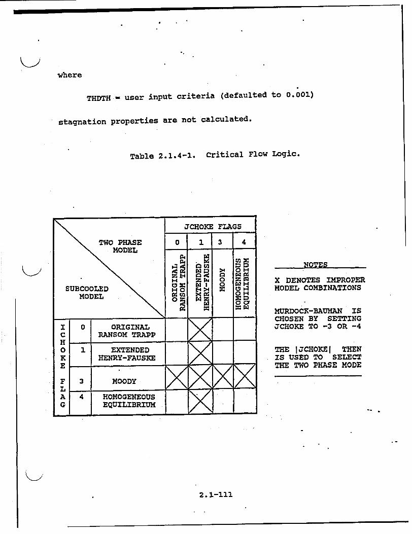
K>where

THDTH = user input criteria (defaulted to 0.001)

stagnation properties are not calculated.

Table 2.1.4-1. Critical Flow Logic.

NOTES

X DENOTES IMPROPER

MODEL COMBINATIONS

MURDOCK-BAUMAN IS CHOSEN BY SETTING JCHOKE TO -3 OR -4

THE j JCHOKE THEN IS USED TO SELECT THE TWO PHASE MODE

2.1-111

J

2.1.4-2. Abrupt Areg Chanae

The general reactor system contains -piping networks with many

sudden area. changes and orifices. To apply the RELAP5

hydrodynamic model to such systems, analytical models for these components have been developed. 8 1 . The basicý hydrodynamic model

is formulated for slowly varying (continuous) flow area variations; therefore, special models are not required for this case.

The abrupt area change model discussed here and developed in detail in Reference 81, is based on the Bourda-Carnot 8 2

formulation for a sudden enlargement and standard pipe flow relations, including the vena-contracta effect for a sudden contraction or an orifice or both. Quasi-steady continuity and momentum balances are employed at points of abrupt area change. The numerical implementation of these balances is such that hydrodynamic losses are independent of upstream and downstream nodalization. In effect, the quasi-steady balances are employed `_2 as jump- conditions that couple fluid components having abrupt changes in cross-sectional area. This coupling process is achieved without change to the* basic linear semi-implicit

numerical time-advancement scheme.

Abrupt Area Change Modeling Assumptions

The basic assumption used for the transient calculation of twophase flow in flow passages with points of abrupt area change is that the transient flow process can be approximated as a quasisteady flow process that is instantaneously satisfied by the upstream and downstream conditions (i.e., transient inertia,..

mass, and energy storage are neglected at abrupt area changes). However, the upstream and downstream flows are treated as f~ully

transient flows.

2.1-112

There are several, bases for the above assumption. A primary

consideration is that available loss correlations are based on

data taken during steady flow processes; however, transient

investigations 8 3 have verified the adequacy of the quasi-steady

assumption. The volume of fluid and associated mass, energy, and

inertia at points of abrupt area change is generally "small

compared with the volume of upstream and downstream fluid

components. The transient mass, energy, and inertia effects are

approximated by lumping them into upstream and downstream flow

volumes. Finally, the quasi-steady approach is consistent with

modeling of other important phenomena in transient codes (i.e.,

heat transfer, pumps, and valves).

Review of Single-Phase Abrupt Area Change Models

The modeling techniques used for dynamic pressure losses

associated with abrupt area change in a single-phase flow are

reviewed briefly before discussing the extension of these methods

to two-phase flows. In a steady incompressible flow, losses at

an area change are modeled by. the inclusion of an appropriate

dynamic head loss term, hL, in the one-dimensional modified

Bernoulli equation

(V2 /2 + P/P)1 (v2 /2 + P/p) 2 + hL 2.1.4-53

The particular form of the dynamic head loss is obtained by

employing the Bourda-Carnot 8 2 assumption for calculating losses

associated with the expansion part of the flow process. Losses

associated with the contracting part of the flow process are

small relative to the expansion losses, and are neglected.

The most general case of an abrupt area change is' a contraction

with an orifice at the point of contraction." . .Such a

configuration is shown in Figure 2.1.4-4. Three area ratios are

used throughout this development. The first is the contraction

2.1-113

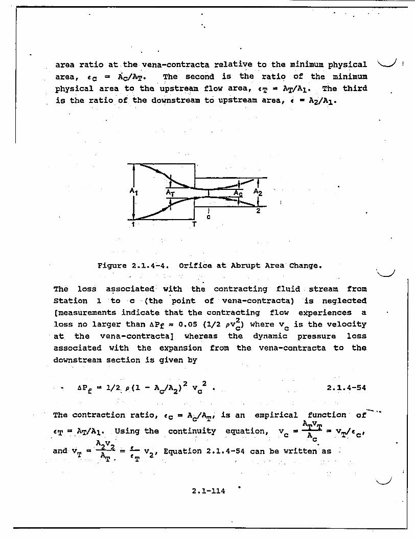
area ratio at the vena-contracta relative to the minimum physical •2

area, Lc = Ac/AT. The second is the ratio of the minimum

physical area to the upstream flow area, 4T = AT/Al. The third

is the ratio of the downstream to upstream area, c - A2 /AI.

Figure 2.1.4-4. Orifice at Abrupt Area Change.

The loss associatedý with the contracting fluid stream from

Station 1 to c (the point of vena-contracta) is neglected

[measurements indicate that the contracting flow experiences a

loss no larger than APf = 0.05 (1/2 pv2) where vc is the velocity

at the vena-contracta] whereas the dynamic pressure loss

associated with the expansion from the vena-contracta to the

downstream section is given by

lap - 1/2 p(1 - Ac/A 2) vC2. 2.1.4-54

The contraction ratio, ec - AIATI is an empirical function of" "

9T =,AT/Al. Using the continuity equation, v AT = VT c + . .. ..... . Ac _ T c C '

A v and VT v v, Equation 2.1.4-54 can be written as

A T .T 2

2.1-114

K)APf 1/ 2 p t 7:T] V_2_ 2 2.1.4-55

Equation 2.1.4-55 is applicable to all the cases of interest.

For a pure. expansion, cT 1i cc - 1, and c > 1; for a

contraction, CT = c < 1 and cc < 1. Each of these is a special

case of Equation 2.1.4-55. The two-phase dynamic pressure loss

model is based on an adaptation of the general single-phase head

loss given by this equation.

Two-Phase Abrupt Area Change Model

The two-phase flow through an abrupt area change is modeled in a

manner very similar to that for single-phase flow by defining

phasic flow areas. The two phases are coupled through the

interphase drag, a common pressure gradient, and the requirement

that the phases coexist in the flow passage.

The one-dimensional phasic. stream-tube momentum equations are

given in section 2.1.1.1. The flow at points of abrupt area

change is -assumed to be quasi-steady and incompressible. In

addition, the terms in the momentum equations due to body force,

wall friction, and mass transfer are assumed to be small in the

region affected by the area change. The interphase drag terms

are retained since the gradient in relative velocity can be large

at points of abrupt area changes.

Equations 2.1.1-5 and 2.1.1-6 can be integrated approximately for

a steady incompressible, smoothly varying flow to obtain modified

Bernoulli-type equations.

2.1-115

(1/2 2 f (/2 ff + p ~ )2 + [" (Vf 1l - vgl) L, St f2 1

+ ( NI'- (V- 2 -g 2) '2 2.1.4-56

and

(1/2 PgVg2 + (1/2 P gvg2 + p,+ [ (!Vg - Vfl) L,

+ N ,. 2 v f 2 ) L2 . 2.1.4-57

where FI' = af ag pf pg Fl. The interphase drag is divided into

two parts associated with the upstream and downstream parts of

the flow affected by the area change.

General Model

Consider the application of Equations 2.1.4-56 and 2.1.4-57 to

the flow of a two-phase fluid through a passage having a

generalized abrupt area change (the flow passage shown in Figure

2.1. 4 - 5 ).a Here, the area AT is the throat or minimum area

associated with an orifice located at the point of the abrupt

area change. Since each phase is governed by a modified

Bernoulli-type equation, it is reasonable to assume that losses

associated with changes in the phasic flow area can be modeled by

separate dynamic pressure loss terms for both the liquid and gas

phases. Hence, we assume that the liquid sustains a loss as if

it alone (except for the interphase drag) were experiencing an'n

area change from afl A1 to afT AT to af2 A2 , and the gas phase

aIn Figure 2.1.4-5,- the flow is* shown as a separated flow for clarity. The models developed are equally applicable to separated and dispersed flow regimes.

2.1-116 *

v •

K>

Gasphase a g, A, ••aTAT :ag2A2•

quid phase 'a, .A

I 2 A_ C

1 T

Figure 2.1.4-5. Schematic Flow of Two-Phase Mixture K>at Abrupt Area Change.

experiences a loss as if it alone were flowing through an area

change from agI Al to UgT AT to Og2 A2 . The area changes for

each phase are the phasic area changes (see Figure 2.1.4-5).

When the losses for these respective area changes (based on the

Bourda-Carnot model and given by Equation 2.1.4-55) are added to

Equations 2.1.4-56 and 2.1.4-57, the following phasic momentum

equations are obtained

1/2 pfVf 2 + 1/2 p-fvf2 + + 1/2 p f I I1 2 1 *fT € fc

(v 2)+ (f, - Vgi) L, + (vt ( - Lg2

2.1.4-58

2.1-117

and

1/ 2 r2 P1 3 1- a2 e 2 1/2 P gg + P) 1= 1/2 pgVg + P)2+ i Pg1 - T Cgc 'TJ (Vj 2 + (Vgl - vf1 ) L1 + (L 2 (vg2 - Vf2) L2 "

2.1.4-59

These phasic momentum equations are used across an abrupt area change. In Equations 2.1.4-58 and 2.1.4-59, ifc and cgc are the same tabular function of area ratio as in the single-phase case except that the area ratios .used are the phasic area ratios

CfT = (*fT"fl) "T 2.1.4-60

and

I (a£Jgl) 'T 2.1.4-61

respectively., The area ratios, e A2 /A 1 and cT - AT/Al, are the same as for single-phase flow.

The interphase drag effects' in Equations 2.1.4-58 and 2.1.4-59 are important. These terms govern the amount of slip induced by an abrupt area change, and if they are omitted, the model will always predict a slip at the area change appropriate to a completely separated flow situation and give erroneous results for a dispersed flow.

Model Application

A few remarks concerning the way Equations 2.1.4-58 and 2.1.4-59 are applied to expansions and contractions, both with and without an orifice, are necessary. In a single-phase steady flow situation, given the upstream conditions, vI and PI, using the

2.1-118

I

K>

+ Ea2 (Vf2 - Vg 2 ) L2 2.1.4-62

andVg2 2

(1/2 p gVg 2 + 1)3 i 1/2 P 4V"2 + P)J2 + 1/2 pg - g (V,2 )2

+ [F -] (Vg 2 !g IJg - vf 2 ) L 2 . 2.1.4-63

These two equations with the incompressible continuity equations

2.1.4-64affliA = *f2vf2A2

and

ag 1 Vg 1 A1 = Og 2 Vg 2 A22.1.4-65

are a system of four equations having four unknowns,

*f2 (ag2 a1 - tf2) , vf 2 , Vg2, and P2 , in terms of the upstream

conditions, a0 f (agl = 1 - Of,), Vfl, Vgl, and P 1 - (The

2.1-119

continuity equation (viA1 - v2 A2 ) and Equation 2.1.4-53 one can

solve for v 2 and P2 . Equations 2.1.4-58 and 2.1.4-59 along with

the two phasic continuity equations can be used in a similar

manner except now the downstream void. fraction is an additibnal

unknown which must be determined.

Expansion

For the purpose of explanation, consider the case of an ekpansion

(*fT = alf, c > 0, cT -1, efc = cgc = 1, FI' 1 - 0, L 1 - 0)" for

which Equations 2.1.4-58 and 2.1.4-59 reduce to

(1/2 Pfvf2 + = (1/2 Pvf2 + + 1/2 pf1 (v f2)2

interphase drag, FI', is a 'known function of the flow

properties.) It is- important to note that the downstream value

of the liquid fraction (af2x )is. an additional unknown compared

with the single-phase case and is determined (with the downstream

velocities and pressure) by simultaneous solution of Equations

2.1.4-62 through 2.1.4-65 without additional assumptions. It is

reassuring that by taking a proper linear combination of

Equations 2.1.4-58 and 2.1.4-59 the usual overall momentum

balance obtained using the Bourda-Carnot 8 2 assumption can be

obtained.8 4 -8 5

If, as in the cited literature,84-87 only the overall momentum

balance is used at an expansion, there will be an insufficient

number of equations to determine all the downstream flow

parameters, af2, vf2, Vg2, and P2- The indeterminacy has been

overcome in cited works by means of several different assumptions

concerning the downstream void fraction.a In the model developed

here (Equations 2.1.4-62 and 2.1.4-63), division of the overall

loss into liquid and gas parts, respectively, results in

sufficient conditions to determine all downstream flow variables

including af2- In addition, the present model includes force

terms due to interphase drag in Equations 2.1.4-62 and 2.1.4-63,

which are necessary to predict the proper amount of slip and void

redistribution that occur at points of area change.

Contraction

Consider the application of Equations 2.1.4-61 and 2.1.4-62 to a

contraction. To determine both the downstream conditions and

throat conditions from the upstream values of afl(agl), Vfl, Vgl,

and PI, an additional consideration needs to be made. To obtaili

aj* G.7.Collier 8 4 mentions three different assumpti'ons that have been used:. (i cf2 = c9fl, (ii) Of2 is given by a homogeneous model, and (iii) czf2 is given by the Hughmark void fraction correlation.

2.1-120

the throat values, apply the momentum equations valid for the

contracting section of flow (here, the L1 portion of the

interphase force is associated with the contraction), that is,

([1/2 PfVf + p)]1 -(1/2 P fv2 +]T (-] (Vfl - vg,.) Li.

2.1.4-66

(1/2 PgVg 2 + P]1 (1/2 gg 2 + p)T + (] (vg, - vf 3) L1 1

2.1.4-67

af VlAl =~ •fVf ,2.1.4-68 Ofivfil A f~vfTAT 2146

and

Kag 1 Vg 1 A1 o 2.1.4-69

These four equations are solved simultaneously for the values of

afT(agT), VfT, VgT, and PT at the throat 'section (the minimum

physical area). No additional or special assumptions are made

concerning the throat conditions since they follow as a direct

consequence of the unique head loss models for each phase. After

the throat values have been obtained, the conditions at the point

of vena-contracta are established assuming the void fraction is

the same as that at the throat. Thus, efc and cgc are

established using the tabular function in Appendix A of Reference

81 and the throat area ratios, cfT and cgT, defined by Equations

2.1.4-60 and 2.1.4-61. To determine the: downstream values,

Equations 2.1.4-58 and 2.1.4-59 can- be applied directly from

stations 2 to 2 with the throat values known or- the expansion

loss equations can be used from the throat section to. station 2.

Both approaches produce identical downstream solutions. As in

the case of an expansion, because the proper upstream and

2.1-121

downstream interphase drag is included, this modeling approach establishes the phase slip and resulting void redistribution. An orifice at an abrupt area change is treated exactly as the contraction explained above (i.e., with two separate calculations to establish first the throat and then the downstream flow

variables).

Countercurrent Flow

The preceding development. implicitly assumed a cocurrent flow. For countercurrent flow, Equations 2.1.4-58 and 2.1.4-59 are applied exactly as in cocurrent flow except that the upstream sections for the respective phases are located on different sides

of the abrupt area change. The difference appears in how the throat and downstream voids are determined. To determine the throat properties, equations similar to Equations 2.1.4-66 through 2.1.4-67 are used with the upstream values appropriate for each phase. These four equations are then solved for

2fT(*gT), VfT, VgT, and PT- To determine the downstream values for each phase, only the head loss terms are needed for the downstream voids (the downstream vf, Vg, and P do not appear). For countercurrent flow, these voids are set* such that the

downstream void of each phase plus the upstream void of the opposite phase adds to one (both phases together must fill the flow channel). With the throat and downstream voids now known, Equations 2.1.4-58 and 2.1.4-59 can be used directly to determine the total loss for each phase at the abrupt area change.

2.1.4.3. Crossflow Junction

The RELAPS numerical scheme is generally formulated using one:

dimensional elements. However, there are several applications where an approximate treatment of crossflow provides an improved physical simulation. Three different applications- for a crossflow formulation are described in the following paragraphs.

2.1-122

KJ.

The first application concerns a small crossflow between two

essentially axial flow streams. This situation is typical of

regions such as a reactor core or a steam generator because the

component geometry provides a large resistance to crossflow and a

small resistance to axial flow. Hence, simplified crossflow

momentum equations can be used to couple a hot flow channel to a

bulk flow channel.

The second application of a crossflow junction is to provide a

tee model. In this case, the momentum flux in the side branch is

assumed to be perpendicular to the main stream and thus the nain

stream momentum flux does not contribute to the cross flow

momentum formulation.

The third application is modeling of leak flow paths. In this

case, the flow is small and governed primarily by pressure

differential, gravity, and flow resistance. Thus, the momentum

K> flux terms can be neglected.

The vapor momentum finite difference equation used in the basic

numerical scheme is

Pc~ vnj Atý+1&ý)[V) )n a j [ 1 x +[V, t + viscous

9 g9 j 2g 3 Lg, L gj TERMS

, -n(~~ Pn+1 l) at

',g~n[[FWGn + FWG L) _Ax + HLossGI n+l~

[O iljL K L4j Vg 1 t - ctgg nl~ F1G n+l n+jlax a + (aggin xxa

LggJ) j - Vf,3J ~ ~ x~~ ~xA

"+ ADDED MASS + MASS TRANSFER MOMENTUM

"+ HORIZONTAL STRATIFIED PRESSURE GRADIENT EFFECT, 2.1.4-70

2.1-123

where

A xj ½A + 2.1.4-71 =a2(Axk + Axl). *

A parallel equation holds for the liquid phase. It should be noted that the momentum Equation 2.1.4-70 is in reality the sum of half the K cell momentum plus half the L cell momentum. This is the reason for Equation 2.1.4-71.

There are two areas in which the crossflow modeling affects the numerical scheme. One concerns the approximations made in the junction momentiim equations; the other concerns the volume average velocities in a volume.

If the junction is to model crossflow perpendicular to the main or axial-flow direction then the volume average velocity in the K and L cells, which represent the axial flow velocity, should not include crossflow junction velocity components. For the simple leak flow situation shown in Figure 2.1.4-6, this requires that

Figure 2.1.4-6. Simplified Tee Crossflow.

2.1-124

vJ,3 not be included in the volume average (axial) velocity

calculation for cell L.

The second area of numerical modification relates to the reduced

form of the momontum equations to be used at a crossflow

junction. Xn crossflow junctions, the cross product momentum flux

terms are neglected, that is, there is no x-direction transport

of momentum due to the y velocity.

For the case of a small crossflow junction between two axial-flow

streams (J 2 in Figure 2.1.4-7) all the geometric input (AVOL, DX,

DZ) for both of the volumes relates to the axial flow direction

as does the wall drag and code calculated form losses. Since the

crossflow has a different flow geometry and resistance (for

example, crossflow resistance in a rod bundle) the friction and

form losses must be user input and must be appropriate for the

crossflow direction geometry. For crossflow junctions the user

input form losses should include all crossflow resistance (form

losses and wall drag). The normal terms representing wall drag

and abrupt area change losses are not included in the formulation

of the momentum equation at a crossflow junction as these refer

to the axial properties of the K and L volumes.

"VI " V2

J2

" -J4 - J5

Figure 2.1.4-7. Modeling of Crossflows or Leak.

2.1-125

Since the connecting K and L volumes are assumed to be predominately axial-flow volumes, the crossflow junction momentum flux (related to the axial volume velocity in K and L) is neglected along with the associated numerical viscous term. In addition, the horizontal stratified pressure gradient is neglected.,

All lengths and elevation changes in the one-dimensional representation are based upon the axial geometry of the K and L volumes and the crossflow junction is assumed to be perpendicular to the axial direction and of zero elevation change, thus, no gravity force term is included.

The resulting vapor momentum finite difference equation for a crossflow junction is

( jn(vnn vn nK

-(a gPg) HOSSGQ vn+4 At

a (apg)jn FIG n (vn+1 v n+1laxti

+ ADDED MASS + MASS TRANSFER MOMENTUM. 2.1.4-72

A similar equation can be written for the liquid phase. In Equation 2.1.4-72, HLOSSGn contains only the user-input crossflow resistance. The Ax term that is used to estimate the inertial length associated with crossflow is defined using the diameters

of volumes K and L,

Rev. 4 2.1-126 9/99

K-)

! j 2 [D(K) + D(L)] • 2.1.4-73

A special void-dependent form loss option of the full crossflow

model has been added for certain multi-core channel applications.

This option allows the user to alter the input constant form loss

coefficient based on the void fraction' in the upstream volume.

The specific applications are possibly multi-channel core

analyses such as SBLOCA scenarios with significant core

uncovering or future multi-channel BEACH reflooding calculations.

This model allows the regions of the core covered by a two-phase

mixture or pool to have a resistance that is different from that

in the uncovered or steam region. The croseflow resistance

changes can alter the volume-average axial velocities that are

used to determine the core surface heat transfer. Any cross flow

is excluded from the volume average velocity used for heat

transfer.

The model uses the input form loss coefficients whenever the

upstream steam void fraction is less than a user-supplied minimum

void fraction value given as 0•,.r=o,,- The model allows user

input of a forward, Mf-fowrd, and reverse, Mj-rev.r.e, crossflow

resistance multiplier when the upstream steam void fraction is

greater than the maximum user-input void fraction,

Linear interpolation is used to determine the multiplicative

factor when the void fraction is between minimum and maximum

input void fractions as indicated in the following equations.

For the forward flow direction (from Volume K to Volume L),

If a. (K)" < otaf-I,-•cos, Kj• n , forward

If caax--xco, 151 (K) Mi, " U l forward * MX-forad

If n.-X.os,, S a. (• ) < a - aKjU.n m Kj= forward * MX1 intrp

2.1.4-73.1

Rev. 4 2.1-126.1 9/99

where

MkCnterp - (. - MK-fr, ij ) i0 cr }* rC,, M I (K)J/ Cfin- - c•f-AX.KCZOSS,

and Kj, -ferd is the user-supplied forward loss coefficient

specified in this Junction input.

The equation for the reverse flow direction (from Volume L to Volume K) is similar.

If % CL) <C 06ID..cross F - Kiua reverse

If 4Maz-KcroS .1 Cf. C(L) KJqg - K1 ravirso * Mr-reverso

If Crn.,.cro s c (L) < a x-•xcraos KU, " KJun reverse * MXr intrp

2.1.4-73.2 where

MMc Lntrp - 1 - (1 - M-reers, ) E -cr°, - a. (L) ] / [.,_,o,, -C% .xcrO,,)

and Klu. rov, is the user-supplied reverse loss coefficient specified in this junction input.

The code performs several input checks to ensure that the user input will not cause code failures. These checks include tests to see if the input form loss multipliers are greater than zero. The minimum void fraction must be greater than zero and less than the maximum void fraction input. The maximum void fraction must be less than or equal to one.

The crossflow option can be used with the crossflow junction perpendicular to the axial flow in Volume L (or K) but parallel

Rev. 4 2.1-i26.2 9/99

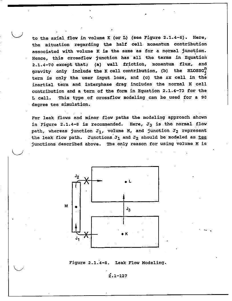
to the axial flow in volume K (or L) (see Figure 2.1.4-6). Here,

the situation' regarding the half cell momentum contribution

associated with volume K is the same as for a normal Junction.

Hence, this crossflow junction has all the terms in Equation

2.1.4-70 except that; (a) wall friction, momentum flux, and

gravity only include the K cell contribution, (b) the HLOSSGn

term is only the user input loss, and (c) the Ax cell in the

inertial term and interphase drag includes the normal K cell

contribution and a term of the form in Equation 2.1.4-73 for the

L cell. This type of crossflow modeling can be used for a 90

degree tee simulation.

For leak flows and minor flow paths the modeling approach shown

in Figure 2.1.4-8 is recommended. Here, 33 is the normal flow

path, whereas junction 71, volume M, and Junction L2 represent

the leak flow path. Junctions.JLI and J 2 should be modeled as tee

junctions described above. The only reason for using volume M is

K-)

M

Figure 2.1.4-8. Leak Flow Modeling.

i. 1-127

to obtain a correct representation of the gravity head from K to L. If a crossflow junction were modeled directly between volumes

K and o L- then there would be no gravity head in the leak flow

jfunction equation. Leak paths may also be modeled using a

crossflow junction that is perpendicular to both the K and L volumes when- the leak flow is between volumes having the same

volume center elevation.

2.1.4.4. Branch

The branch component is a model designed for convenient interconnection of hydrodynamic components. The identical result can be obtained by using a single volume component and several

single junction' components. Thus the branch is a separate

component only in the input processing scheme.

In RELAPS/MOD2 the crossflow junction has been added in which the

junction velocities *are assumed to be normal to the onedimensional flow path of the hydrodynamic volume. Thus, the \1

branch component can include multiple connections at the inlet,

outlet, or in the crossflowdirection.

Specialized modeling considerations are applied to any volume

having multiple junctions connected at either volume end (the

ends of a hydrodynamic volume are the inlet and outlet as defined

in section 2.1.1.1).

These special calculations include both the method for

calculating the volume average velocities and the method for partitioning the volume cross-sectional area between the multiple

inlet or multiple outlet junctions. The partitioned volume areas

are used both in the abrupt area change model to calculate

kinetic loss factors and in the momentum equations to simulate

the stream-tube area.

2.1-128

In applications, the multiple junction and crossflow models are

used in three distinct ways to model branching flows. These are

the one-dimensional branching, a tee branch, and a crossflow

branch. Combination of the three basic brinches may also occur.

Each of the three basic models will be discussed in turn.

One-Dimensional Branchina

This basic branch model is consistent with the one-dimensional

approximation for a piping network and assumes that

multidimensional effects at branches are small compared to system

interaction effects. In the case of branched flows that occur in

headers or plena, the model gives an accurate physical

description of the flow division or merging process and the one

dimensional branch model is intended primarily for use in

modeling such branched flows. Examples of such situations in LWR

systems are flow division at the core inlet if parallel flow

paths through the core are modeled, steam generator inlet and

> outlet plena when several parallel tube groups are modeled (for

the effect of tube height and length), or at a wye connection.

The one-dimensional branch is illustrated in Figure 2.1.4-9 for a

volume having two inlet junctions and *one outlet junction.' The.

junctions Jl and U2 are the inlet junctions and junction X3 is

the outlet junction. The multiple flows are assumed to merge in

such a way that they come to the common velocity equal to the

inlet volume average velocity for volume V3 . The volume cross

sectional area is then divided in proportion to the volume flow

of the respective inlet junctions. This method of apportioning

volume cross-sectional area satisfies continuity but does not

conserve momentum, particularly for high velocity differences

between the merging streams (for flow splitting, however, the

method does preserve momentum). For this reason the special Jet

mixer component was developed' for merging flows liaving high

relative velocities such as in a jet pump. 'The jet-mixer can be

used for one-dimensional mixing, but is limited to two inlet

2.1-129

streams and *a single outlet stream (see Appendix A for a reference to the jet-mixer model). The volume partitioned areas are calculated as follows

[ nc~J (vf)nli + I (ggqjI (v,) I]AjAk (AK) = . 2.1.4-74

iJ1 V

Figure 2.1.4-9. Oxie-Dimensional Branch.

The apportioned volume areas for each junction are used with the abrupt area change model, section 2.1.4.2, to calculate energy loss coefficients for the liquid and vapor streams at each junction.

Ninety-Dearee Tee Model

The crossflow junction (see section 2.1.4.3) is used to form a 90-degree tee as shown in Figure 2.1.4-6. In this particular application the side connection to the tee is modeled using a. junctionýin which only one-half of the junction momentum equation has the crossflow form (the half of the junction' J 3 associated with volume VL is a crossflow junction and is designated by an X, see Figure 2.1.4-6).

2.1-130

No special component is provided to accomplish the input

associated with a model such as illustrated in Figure 2.1.4-6.

The volume VL may be specified as a branch with the associated

junctions or as a single volume with single junctions used to

specify the connecting junctions. In either case, junctions J1

and T2 should be specified as smooth unless actual abrupt changes

in area occur at either junction. The junction J3 should be

specified as smooth with a user input form loss factor to account

for the turning and entrance losses. In addition, junction J 3

must be specified so that the half of the junction associated

with volume VL is modeled as a crossflow junction and the half

associated with volume VK is a normal junction. These options

are specified through input of junction control flags.

It is also possible to model a 90-degree tee with the RELAPS/MOD2

code, however, unphysical numerical results may be obtained.

Thus, the 90-degree tee model described previously is recommended

and is a closer approximation to the actual fluid momentum

interaction which occurs at a tee.

Gravity Effects at a Tee

In some branching situations where the through flow is small or

where the flow is constrained by the geometry, body force effects

may be significant. Examples that occur in PWR systems are the

cold leg connections to the inlet annulus and downcomer, and the

hot leg connection to the upper plenum and core. This type of

branched flow is modeled as shown in Figure 2.1.4-10. Here the

vertical direction is modeled as the through-flow direction

(indicated by the volume orientation arrows). The cold or hot

leg connections are modeled by crossflow junctions. The through

flow direction of volume V3 is chosen to correspond to the major

flow path. In the case of a PWR inlet annulus through-flow in

the horizontal direction is inhibited by the annular structure

and in the case of the upper plenum to core connection the area

for flow in the vertical direction is large compared to the flow

2.1-131

area in the horizontal direction. Some judgment is required to select the orientation. However, the crossflow branch connection will permit through-flow in the horizontal direction but with some accompanying pressure rise and drop associated with the fact that the momentum flux terms are neglected in the crossflow part of the junction.

Figure 2.1.4-10. Gravity Effects on a Tee.

The model illustrated in Figure 2.1.4-10 has the additional advantage that the effect of vertical void gradients in the flow out of the horizontal connections may be more sharply defined as a result of the central volume, V3 , which has a vertical height equal to the diameter of branch volumes V1 and V4 .

No special component model is provided for modeling the vertical . tee and either a branch or a single volume may be used for volume

V3. The branch component is more convenient sincd all junctions -connecting to volume V3 can be specified with the branch

component.

2.1-132

6

Crosfalow Branch

A fourth type of branch flow path can be created by the use of a

crossflow Junction to couple two volumes. This type of branch is

used* to model crossflow between columns having centers at the

same vertical elevation. The crossflow Junction is assumed to

have no elevation change; thus, one limitation of this type of

branch is that the volume centers that are coupled must be at the

same elevation. If volumes of differing elevation are coupled,

an input processing error will occur in the loop elevation

checking routines. The application of the crossflow junction for

crossflow or leak path modeling is illustrated in Figure 2.1.4-7.

The length scale associated with the crossflow Junction is one

half the diamter of the L volume. This length is only used for

modeling the fluid inertia terms in the momentum equation and is

always assumed to lie in a horizontal plane.

The pure crossflow branch is most easily modeled using a single

junction component for the crossflow junction. However, either

volume, V1 or V2 in Figure 2.1.4-7, can be modeled' using the

branch component and specifying the coupling junctions with that

component.

2.1.4.5. Countercurrent rlow Limit (CCFL) Model

During the reflux condensation period of a small break LOCA

transient in a PWR with U-tube steam generator, countercurrent

flow limitation (CCFL) often will occur at the hot leg bend and 34

at the U-tube inlet. The Wallis CCFL correlation is added to

calculate the steam and liquid flow rates for certain RELAP5

junctions. The applicability of the CCFL model -is limited to the

volume and junction configurations shown in Figure 2.1.4-11, in

which K and L are RELAP5 volumes, the junction J is from the exit

of volume K to the inlet of volume L, and AZ is the elevation

change of each volume.

Rev. 2 2.1-133 8/92

a) AZ(K)>O & AZ (L) >0

yiL

b) AZ(K)<o & AZ (L) <o

c) AZ(K)-O & AZ (L) >0

LW d) AZ(K)<O a

AZ (L) -0

Figure 2.1.4-11. Volumes. and Junction Configurations Available for CCFL Model.

The general form of the Wallis CCFL correlation is:

2.1.4-75

where m is the negative slope and c is the y-intercept, respectively, of a plot of J; g j The dimensionless gas

f * ar e fi n e d b y flux, -;,and the liquid flux, j f, are defined by

g 9 Jg j OPf - Pg) 2.1.4-76

J* = if [ Pf - 1/2 if g j(Pf - Pg9) 2.1.4-77

respectively, where j is the gas superficial velocity, if is the

liquid superficial velocity, and D.j is the junction hydraulic diameter.

Rev. 2 2.1-133.1 8/92

KJ.

and

Jg1/2 + m jf /

With regard to the solution method, if the CCFL model is

requested by the user, the coding checks if countercurrent flow

exists and if the liquid downflow: exceeds the limit imposed by

equation 2.1.4-75. If this is true, the. sum momentum equation

and the flooding limit equation is applied as has been done in

RELAP5/MOD3.144 The code's difference equation is replaced with

the flooding limit equation during.the semi-implicit intermediate

velocity calculation (Subroutine VEXPLT). The difference

equation contains the interphase friction, whereas the sum

equation does not. This method is advantangeous in that the

phasic velocities still must satisfy the the sum equation which

contains gravity and pressure terms. The numerical form of

Equation 2.1.4-75 needed by the code is obtained by letting Cg M

jg*Vg and c * f/vf solving for mj /2, and squaring the

equation. This results in

m2 cn vn+l =c2 2c n 1/2 n+l 1/ 2 + cn n+l

f ,j f 2 c ,) (V,j g,j Vg,j.

2.1. 4-78

vn+1. 1/2gie Linearization of (V g 1/j

(v n+l) 1/2= (vn ) 1/2 + n )-1/ 2 (n+- vn 2.1.4-79 g, g,j + 2 Vg,)j (Vg,)j j 2.

and substitution into equation 2.1.4-75 produces

m2 n n+l c 1/2 n)-1/2 - n n+1 c~ ~ ,.v~ + [ c -(n f~j f~j9,J) V4,) 0,J 3] g,j

c 2 - c (c,j) 1 / 2 (vg n 1/2. 2.1.4-80

The above method can be used when both the RELAP5 momentum

equations and the CCFL correlation predict countercurrbnt, flow.

In situations where RELAP5 predicts countercurrent flow and the

Rev. 2 2.1-133.2 8/92

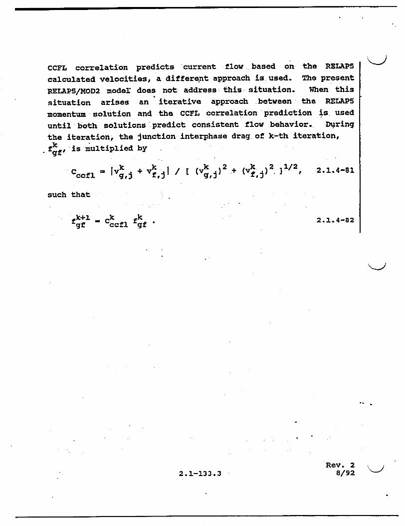
CCFL correlation predicts current flow based on the RELAP5

calculated velocities, a different approach is used. The present

RELAPS/MOD2 moder does not address this situation. When this

situation arises an iterative approach between the RELAP5

momentum solution'and the CCFL correlation prediction is. used

until both solutions predict consistent flow behavior. DWring

the iteration, the junction interphase drag of k-th iteration,

fgf is multiplied by

k k vk 2 k 2 1/2 C~~~ ccf V 1 I iVjj +gv-I)j 2.1.4-81

such that

f k+l . ck fk gf ccfl gf 2.1.4-82

Rev. 22.1-133.3

`KU

K-)

This page intentionally left blank.

Rev. 2

2.1-133.4 8/92

2.1.5. Special Component Models

RELAPS consists of a variety of generic models which are used to build system models. The general philosophy has been to avoid system component models such as pressurizer, steam generator, core, etc. However, certain subsystem components are unavoidable due to unique processes or performance. RELAP5 contains models for subsystem components such as a separator, pump, valve, and accumulator. A summary of each of these models is included here.

2.1.5.1. Separator

The RELAP5 separator model is a nonmechanistic or 1 l;boxmodel consisting of a special volume with junction flows as pictured in Figure 2.1.5-1. A steam-water inflowing mixture is separated by defining the quality of the outflow streams using empirical functions. No attempt is made to model the actual separation

process from first principles.

The separator vapor outlet performance is defined by means of a special function for the vapor'void fraction at J1. The donored junction vapor void fraction used to flux mass through the steam outlet is related to the vapor void fraction in the separator volume using the curve in Figure 2.1.5-2. For separator volume void fractions above the value of VOVER (an input parameter) a perfect separation is assumed and pure vapor is fluxed out junction J1. For separator volume void fractions less than VOVER a two-phase mixture is fluxed out. The VOVER parameter governs the vapor void fraction of the outflow. If VOVER is small the vapor outflow corresponds to an ideal separator. IF VOVER equals 1.0 the vapor outlet junction behaves as a normal junction and the vapor outlet junction void fraction is equal to the separator volume average void fraction.

2.1-134

J 1 --Vapor outlet

J 3 -Separator Inlet junction

J2 -Llquld fallback junction

Figure 2.1.5-1. Typical Separator Volume and Junctions.

The flow of the separator liquid drain junction is modeled in a

manner similar to the steam outlet except pure liquid outflow is

assumed when the volume void fraction is less than the value of

VUNDER, see Figure 2.1.5-3. Normal donored fluxes are used for

the separator inlet junction. Although the void fractions used

to flux mass and energy from the separator volumes are modified,

the normal junction momentum equations are used to calculate the

flow velocities.

2.1-135

Volume K

ogJ 1 1.0

0.0

Vapor outlet junction

VOVER 1.0 agK

Figure 2.1.5-2. Vapor Outflow Void Donoring.

"OW 21.0

I Liquid fallback junction

0.0

VUNDER 1.0 ajtK

Figure 2.1.5-3. Liquid Fallback Void Donoring.

2.1-136

2.1.5.2. Pump Model

The pump is a volume oriented component and the head developed by

the pump is apportioned equally between the suction and discharge

junctions that connect the pump volume to the system. The pump

model is interfaced with the two fluid hydrodynamic model by

assuming the head developed by the pump is similar to a body

force. Thus, the head term appears in the mixture momentum

equation, but like the gravity body force, it does not appear in

the momentum difference equation used in RELAP5. The term that

is added to the mixture momentum equation is

2 PgH 2.1.5-1

where H is the total head rise' of the pump (m), p is the fluid

density (kg/m3 ), and g is the acceleration due to gravity (m/s 2 ).

The factor 1/2 is needed because the term is applied at both the

suction and discharge junctions.

In the semi-implicit numerical scheme, the pump is coupled

explicitly so the numerical equivalent of Equation 2.1.5-1 is

•n g H n at ,2.1.5-2 2 pg

where the n designates the previous time level and At is the time

integration interval. This term is added to the right side of

the mixture momentum equation.

In the nearly-implicit numerical scheme, the pump is coupled

implicitly by way of its dependence on the volumetric flow rate

(Q). It is assumed that the head depends on the-volumetric flow

rate, and a first order Taylor series expansion is used

2. 1-137

Hn+l* n _ = n + _]n .n+l 2.1.5-3

Thus, the numerical equivalent of Equation 2.1.5-1 in the

nearly-implicitýscheme is

2 Pg n+_ + 2 2.1.5-4

This term is added to the right side of the mixture momentum

equation, which uses the linear implicit convection term from

NUREG-4312 1 sections 3.1.1.4 and 3.1.1.7.

The pump dissipation is calculated for the pump volume as

S- a (a fPfv f + agpgVg) A 2.1 .5-5

where r is the pump torque and w is the pump speed.

This term is evaluated explicitly in both the semi-implicit and

nearly-implicit schemes, and it is partitioned between the liquid

and vapor thermal energy equations in such a way that the rise in

temperature due to dissipation is equal in each phase (the

details of the dissipation mechanism in a two-phase system are

unknown so the assumption is made that the mechanism acts in such

a way that thermal equilibrium between the phases is maintained

without phase change). Thus, the terms that are added to the

right sides of the liquid and vapor thermal energy equations, are

[n ný_ _qn n n-;n n n-g An, An-, Cnp

n f r + at v

- n Cf n n nnC2 t fPf C pf + a 9g pg 2.1.5-6

2.1-138

and

n n n n jn nc• nn

af Pn Cpf + np Pn 2.1.5-7 f~ 90 9 ~

respectively.

The pump head, H, and torque, r, are defined by means of an

empirical homologous pump performance model and the pump speed,

w, is defined by a pump drive model. The derivative of the pump

head with respect to the volumetric flow rate, dH/dQ, is obtained

from the empirical homologous pump performance model using the

assumption that the pump speed is constant.

Centrifugal Pump Performance Model

The basic pump performance data must be generated experimentally.

Analytical programs have beeh developed that are reasonably

successful in predicting near design pump performance for

single-phase fluids. For off design operation or for operation

with a two-phase fluid, the problems of analytical pump

performance prediction are nearly insurmountable. The basic

parameters that characterize the pump performance are the

rotational speed, w or N, the volumetric through flow, Q, the

head rise, H, and the shaft torque, . The relationship between

these four parameters can be uniquely displayed by a

four-quadrant representation of such data. A typical four

quadrant curve is shown in Figure 2.1.5-4. Both positive and

negative values for each of the four parameters are represented.

The disadvantages in using such a data map for numerical purposes

are the need for two-dimensional interpolation, the large number

of points needed to define the entire range, and the fact that

the map is infinite in extent. These objections can be largely

2.1-139

overcome by use of a homologous transformation based on the "•d centrifugal pump similarity relationships. Such a transformation

collapses the four quadrant data onto a single bounded

dimensionless curve having eight basic octants. Typical homologous curves for the head and torque are illustrated. in Figures 2.1.5-5 and 2.1.5-6 respectively where' or, QR, HR, and

"rR are the rated values for the pump speed, volumetric flow

rate, head, and torque, respectively. The homologous transformation is not unique and not all points of Figure 2.1.5

4 lie on the curves of Figures 2.1.5-5, and 2.1.5-6. However, the data are closely grouped and the single curve is a good approximation for the global pump performance.

The pump model allows the user the option of accounting for cavitation or two-phase degradation effects on pump performance. The user must supply a separate set of homologous, two-phase curves for head and torque that are in the form of difference curves. Difference curves are used because analysis of available <J two-phase pump data indicated that when the fluid being pumped had a void fraction between 0.2 and 0.9, little head was developed by the pump being tested. Outside this range of void fraction, the pump developed head varied from zero to undegraded single-phase performance. To consider the degraded performance,

a set of dimensionless homologous curves was fit to the head data. Thus the fully-degraded two-phase head was expressed as a function of the standard pump model arguments.

To considqr the ranges of void fraction where the pump was able to develop head (0 to 0.2 and 0.9 to 1.0), a multiplier as a function of void fraction was used. The multiplier varied from 0 to about 1.0 as the void fraction varied from 0 to 0.2, and the

multiplier varied from about 1.0 to 0 as the void fraction varied from 0.9 to 1.0.

2.1-140

-- Constant head, H Constant torque, -'

-rpm

ý-ý Figure 2.1.5-4. Typical Pump Characteristic Four-Quadrant Curves.

2.1-141

K>

hlct

cIv

-1.0 vla/

h/v2

ca= l(/W R (speed ratio) h = HIHR (head ratio)

v = 0 /OR (flow ratio)

,-1.0

Figure 2.1.5-5. Typical Pump Homologous Head Curves.

2.1-142

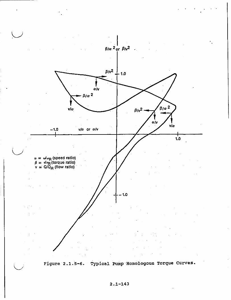
K>f31ct2 or 2/v 2

p/V2

vla,

-1.0

= (= wR (speed ratio) 7= /IR (torque ratio)

v = QIQR (flow ratio)

1.0

1.0

1.0

Figure 2.1.5-6. Typical Pump Homologous Torque Curves.

2.1-143

K>

I

Available pump data from the 1-1/2 Loop Model Semiscale and

Westinghouse Canada Limited (WCL) experiments were used in

developing the-two-phase pump data. Assumptions inherent in the

pump model for two-phase flow include:

1. The head multiplier, MH(ag), determined empirically

for the normal operating region of the pump, is also

valid as an interpolating factor in all other

operating regions.

2. The relationship of the two-phase to the single-phase

behavior of the Semiscale pumptis applicable to large

reactor pumps. This assumes that the pump model of

two-phase flow is independent of pump specific speed.

The single-phase pump head (dimensionless) curve for the

Semiscale pump is shown in Figure 2.1.5-7 and the fully degraded two-phase pump head curves are' shown in Figure 2.1.5-8. These <2 represent complete pump characteristics (except for the reverse

pump fully degraded region) for the Semiscale pump operating under two-phase conditions with the average of the void fractions

of the pump inlet and outlet mixtures between 0.2 and 0.9. The

lines drawn through the data were determined by least square

polynomial fits to the data using known constraints.

A comparison of the two-phase data in Figure 2.1.5-8 with the single-phase data in Figure 2.1.5-7 shows that the two-phase

dimensionless head ratio (h/v 2 or h/a 2 ) is significantly less

than the single-phase dimensionless head ratio for the normal

pump operation region (HAN and HVN). For negative ratios of v/a,

such as those that occur in the HAD region, the pump flow becomes

negative. When the pump flow is negative, the two-phase dimensionless head ratio is greater than the single-phase

dimensionless head ratio. Two-phase. flow friction losses are

2.1-144

K>

Normal pump (+H,+ a N) HVN

Energy dissipation (-0, + a) HAD HVD

Normal turbine (-0,-a') HAT HVT

Reverse pump (+a,-a) HAR HVR

Figure 2.1.5-7. Single-Phase Homologous Head Curves for 1-1/2 Loop MODI Semiscale Pumps.

2.1-145

¾���/

Figure 2.1.5-8. Fully Degraded Two-Phase Homologous Head Curves for 1-1/2 Loop MOD1 Semiscale Pumps.

2.1-146

K> generally greater than single-phase losses, and friction is controlling in this energy dissipation region (HAD). The other

regions of two-phase dimensionless head ratio data show similar

deviations from single-phase data.

Table 2.1.5-1 shows the difference between the single- and

two-phase dimensionless head ratio data as a function of v/a and

a/v for the various pumping regions shown in Figures 2.1.5-7 and

2.1.5-8. The differences shown in Table 2.1.5-1 are for the

eight curve types used for determining pump head.

The head multiplier, MH(ag), and void fraction data shown in

Table 2.1.5-2 were obtained in the following manner. The

Semiscale and WCL pump data9 2 were converted to dimensionless

head ratios of h/a 2 or h/v 2 . Values of the dimensionless head

ratios were obtained for pump speeds and volumetric flow rates

within 50% of the rated speed and flow rate for the pumps. The

difference between the single- and two-phase dimensionless ratios

was developed as a function of the average void fractions for the

pump inlet and outlet mixtures. The difference between the

single- and two-phase dimensionless ratios was then normalized to

a value between 0 and 1.0. The normalized result was tabulated

as a function of the void fraction.

If the two-phase option is selected, the pump head and torque are

calculated from

H H 14 - ME (0g) (HI - H2 0) 2.1.5-8

and

"T" 1 0 -M (ag) (I -10 ) ' 2.1.5-9

2.1-147

where

1ý = single-phase value,

2ý = two-phase, fully degraded value, 0..2 < ag < 0.9,

M = multiplier on difference curve, and

g average volume void fraction.

CentrifuQal Pump Drive Model

The pump torque is used to calculate the pump speed after the

pump has been shut of f by the input trip signal. The speed is

calculated by the-deceleration equation

dca I r 2.1.5-10

The solution of this equation is

t+t t + I2.1.5-11

where

= net torqie,

I moment of inertia,

t = time,

At = time step, and

= angular velocity.

The rate of energy addition to the pump system is given by wr and

has been used in Equation 2.1.5-5 to calculate the pump

dissipation.

2.1-148

Table 2.1.5-1. Semiscale Dimensionless Head Ratio Difference (single-phase minus two-phase) Data.

V a X or

a V

h 2

Curve Type

1 (RIAN)

2 (HVN)

3 (HAD)

x

0.00 0.10 0..20 0.50 0.70 0.90 1.00

0.00 0.10 0.20 0.30 0.40 0.80 0.90 1.00

-1.00 -0.90 -0.80 -0.70 -0.60 -0.50 -0.40 -0.25 -0.10 0.00

or hh

V e

___~u_ Curve Type

0.00 0.82 1.09 1.02 1.01 0.94 1.00

0.00 -0.04 0.00 0.10 0.21 0. V 0.80 1.00

-1.16 -1.24 -1.77 -2.36 -2.79 -2.91 -2.67 -1.69 -0.50

0.00

4 (HVD)

5 (HAT)

6 (HVT)

7 (HAR)

8 (HVR)

2.1-149

-1.16 -0.78 -0.50 -0.31 -0.17 -0.08

0.00 . 0.05 o.b8 0.11

0.00 -0.34 -0.65 -0.95 -1.19 -1.47

0.11 0.13 0.15 0.13 0.07

-0.04 -0.23 -0.51 -0.91 -1.47

x

-1.00 -0.90 -0.80 -0.70 -0.60 -0.50 -0.35 -0.20 -0.10

0.00

0.00 0.20 0.40 0.60 0.80 1.00

0. 00 0.10 0.25 0.40 0.50 0.60 0.70 0.80 0.90 1.00

-1.00 0.00

-1.00 0.00

S

0.00 0.00

0.00 0.00

I

hp S2

Table 2.1.5-2. Head Multiplier and Void Fraction Data. KU1-

MH (a g)

0.00 0.10 0.15 0.24

0.30 0.40 0.60 0.80

0.90 0.96 1.00

.0.00 0.00 0.05 0.80

0.96 0.98 0.97 0.90

0.80 0.50 0.00

The total pump torque is calculated by considering the hydraulic torque from the homologous curves and the pump frictional torque. The net torque with the drive motor shut off is

S= r hy+ rfr I 2.1.5-12

fhy = hydraulic torque and

Sfr = frictional torque.

Pump frictional torque (r'fr = TF) is modeled as a cubic function ofthe pump rotational velocity. The FORTRAN notation for the cubic function is

V VR,2

2.1-150

where

2.1.5-13

SA = Ist , and 2.1.5-14

TF = -SIGN(TFO + TFl.SA + TF2-SA2 + TF3"SA3 , S) , 2.1.5-15

where V is pump rotational velocity, VR is rated pump rotational

velocity, TFO, TF1, TF2, and TF3 are input data, and SIGN is. a

function whose result is the magnitude of the first argument with

the sign of the second argument. An option is available to

specify whether reverse rotation of the pump is allowed.

The electric drive motor will affect the speed behavior of the

pump while the motor remains connected to its power source. The

net torque with the drive motor on is incorporated into the pump

model by adding the value of motor torque, rm' to the torque

summation

"v = hy + 7fr- Tm 2.1.5-16

where the sign of the motor torque is the same as that of the

hydraulic and frictional torque for steady operating conditions,

that is, zero net torque.

Induction motors are used to drive primary coolant pumps. At

constant voltage, the motor torque is an explicit function of

speed. This torque/speed relationship is normally available from

the motor manufacturer.

Motor torque is supplied to the pump model as a.tabular function

of torque versus speed as given by the manufacturer's data. A

typical torque/speed curve for an induction motor is shown in

Figure 2.1.5-9.

The capability to simulate a locked rotor condition of the pump

is included in REIAP5. This option provides for simulation of

the pump rotor lockup as a function of input elapsed time,

2. 1-151

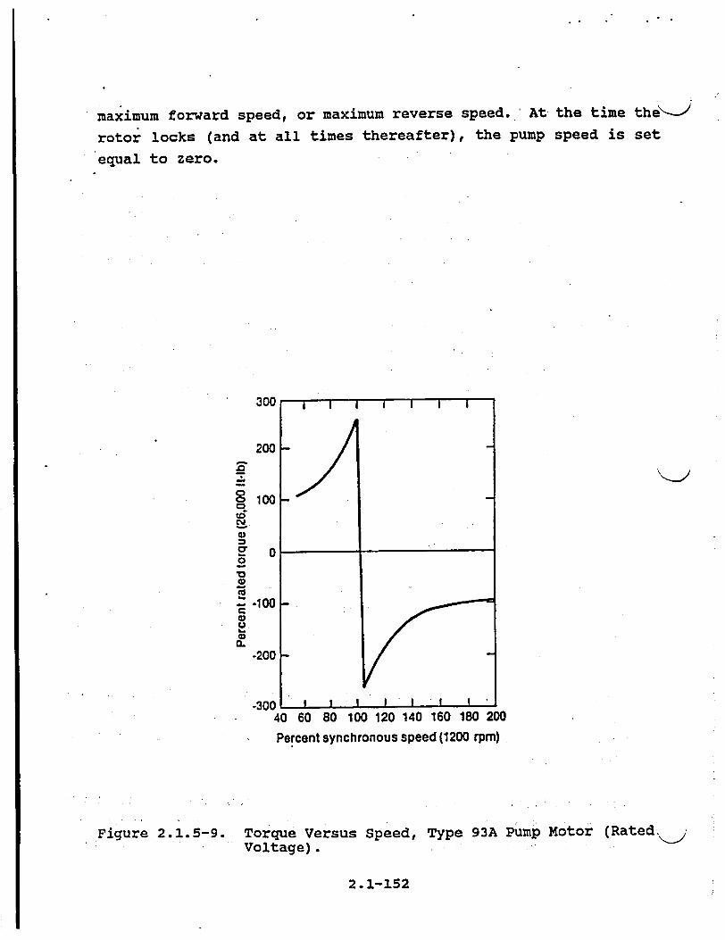
maximum forward speed, or maximum reverse speed. At the time the"--J

rotor locks (and at all times thereafter), the pump speed is set

equal to zero.

300

200

E

0100

S0

E~o

-- 100

CL

-200

-30040 60 80 100 120 140 160 180 200

Percent synchronous speed (1200 rpm)

Figure 2.1.5-9. Torque Versus Speed, Type 93A Pump Motor (Rated, , Voltage).

2.1-152

' I I I I I I

I I I I I I I'

•> 2.1.5.3. Valves

Valves are quasi-steady models that are used either to specify an

option in a system model or to simulate control mechanisms in a

hydrodynamic system. The RELAP5 valve models can be classified

into two categories: (a) valves 'that open or close instantly, and

(b) valves that open or close gradually. Either type can be

operated by control systems or by flow dynamics.

Valves in the first category are trip valves and check valves.

The model for these valves does not include valve inertia or

momentum effects. If the valve is used as a junction with an

abrupt area change, then the abrupt area change model is used to

calculate kinetic loss factors when the valve is open.

Valves in the second category are the inertial swing check valve,

the motor valve, the servo valve, and the relief valve. The

inertial valve and relief valve behavior is modeled using

Newton's second law of motion. The abrupt area change model

controls losses through the valve as the cross-sectional flow

area varies with valve assembly movement. The motor and servo

valve use differential equations to control valve movement.

These two valves include the options to use the abrupt area

change model to calculate losses across the valve or to use flow

coefficients (Cv) input by the user. The Cv's are converted to

energy loss coefficients within the numerical scheme.

Valves are modeled in RELAP5 as junction components'. The types

of valves are defined as follows.

Trip Valve

The operation of a trip valve is solely dependent on the trip

selected. With an appropriate trip, an abrupt full opening or

full closing of the valve will occur. A latch option is also

included for latching the valve in the open or closed position.

2.1-153

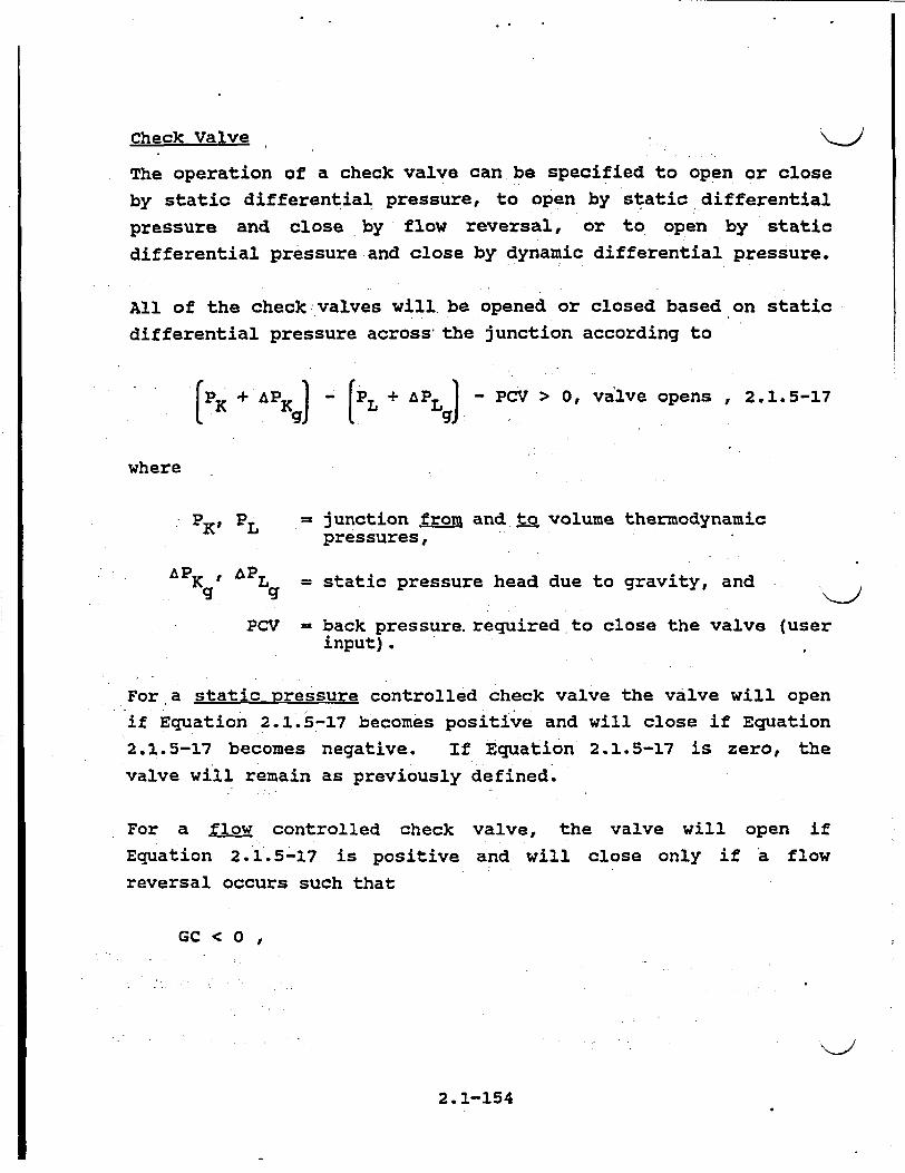
Check Valve

The operation of a check valve can be specified to open or close

by static differential pressure, to open by static differential

pressure and close by flow reversal, or to open by static

differential pressure and close by dynamic differential pressure.

All of the check valves will be opened or closed based on static differential pressure across the junction according to

(PK + A PKgJ - (L +AP LJ PC .V > 0, valve opens ,2.1.5-17

where

•PX' = junction from and to volume thermodynamic pressures,

APK' APLL = static pressure head due to gravity, and g g

PCV = back pressure. required to close the valve (user input).

For a static pressure controlled check valve the valve will open if Equation 2.1.5-17 becomes positive and will close if Equation

2.1.5-17 becomes negative. If Equation 2.1.5-17 is zero, the valve will remain as previously defined.

For a flow controlled check valve, the valve will open if

Equation 2.1.5-17 is positive and will close only if a flow

reversal occurs such that

GC < 0 ,

2.1-154

where GC is the dynamic pressure given as

GC =(IVIV)j = IafqVf + agPgVgl (Cef + * 2.1.5-18

For a dynamic pressure controlled check valve, the valve opens if

Equation 2.1.5-17 is greater than zero. Once the valve is open,

the forces due to pressure differential and momentum hold the

valve open until

K+< 0, valve closes

l = 0, remains as 1 'previously

defined. 2.1.5-19

The terms af and. ag are the junction liquid and vapor volume

fractions, respectively, pf and pg are the junction liquid and

vapor densities, respectively, and vf and vg are the junction

liquid'and vapor velocities, respectively.

All check valves may be initialized as either open or Closed.

Leakage is also allowed if the valve is closed and the abrupt

area change model is used to calculate the valve form losses.

Ihertial Valve

This valve models the motion of the valve flapper assembly in an

inertial type check valve. The abrupt area change model is used

to calculate kinetic form losses assumingqthat the area between

the flapper and the valve seat behaves as an orifice whose area

changes in time as a function of the inertial valve geometry.

The motion of the flapper about the shaft axis is given by

Newton's second law (angular version) as

rI- ,2.1.5-20

2.1-155

where the external torques acting on the valve disk are given by "-.

r = - W L sin(B + ý) - AD L(AP + PBP + Ghead) I 2.1.5-21

where AP is the pressure drop across the valve, and a is the

angular acceleration. Substituting Equation 2.1.5-20 into

Equation 2.1.5-21 gives

Ia = - WL sine - 1rR2 L(AP + PBP + Ghead) I 2.1.5-22

where ý has been dropped by assuming the valve is a horizontal

pipe. Equation 2.1.5-22 is then written in finite-difference

form as

n IwLsinen R2 L(Apn + PBP + Ghead) BP(ead 2.1.5-23

where the superscript, n, indicates the time level, t + n At.

Integrating Equation 2.1.5-23 'with respect to time yields the

angular velocity

n+l = ,n + cnAt 2.1.5-24

Similarly integrating Equation 2.1.5-24 gives the angular

position

,n+l = n + n+l At 2.1.5-25

The throat flow' area for the valve is, set by the following

function

A2wR2 tan(8n+l Athroat =' rR2 6 S 26.565 e > 26.565

2.1.5-2f

2.1-156

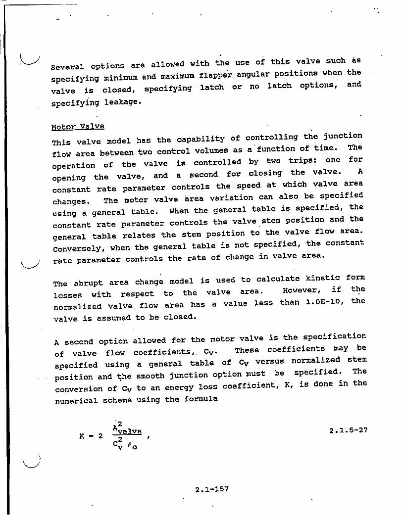
Several options are allowed with the use of this valve such is

specifying minimum and maximum flapper angular positions when the

valve is closed, specifying latch or no latch options, and

specifying leakage.

Motor Valve

This valve model has the capability of controlling the junction

flow area between two control volumes as a function of time. The

operation of the valve is controlled by two trips: one for

opening the valve, and a second for closing the valve. A

constant rate parameter controls the speed at which valve area

changes. The motor valve area variation can also be specified

using a general table. When the general table is specified, the

constant rate parameter controls the valve stem position and the

general table relates the stem position to the valve flow area.

Conversely, when the general table is not specified, the constant

rate parameter controls the rate of change in valve area.

The abrupt area change model is used to calculate kinetic form

losses with respect to the valve area. However, if the

normalized valve flow area has a value less than 1.OE-10, the

valve is assumed to be closed.

A second option allowed for the motor valve is the specification

of valve flow coefficients, Cv. These coefficients may be

specified using a general table of Cv versus normalized stem

position and the smooth junction option must be specified. The

conversion of Cv to an energy loss coefficient, K, is done in the

numerical scheme using the formula

".2 Ava2 ve 2.1.5-27

K 2 2 Cv Po

2.1-157

where

Po = density of water at 288.71 K (60.0 F).

Provisions also exist for applying multipliers to both stem

position and Cv.

servo Valve

The servo valve operation is similar to that for the motor valve.

However, the valve area or stem position is controlled by a control variable rather than by a specified rate parameter. The servo valve also has the same options as the motor valve.

Relief Valve

For thermal-hydraulic analysis of overpressure transients it is necessary to simulate the effects of- relief valves. In particular, it is desirable to model the valve dynamic behavior including simulation of valve flutter and hysteresis effects.

To assist in understanding the relief valve model three schematics of a typical relief valve are shown in Figures 2.1.510, 2.1.5-11, and 2.1.5-12. The three schematics represent the valve in the closed (Figure- 2.1.5-10), partially open (Figure

2.1.5-11), and fully open (Figure 2.1.5-12) modes, respectively. In the schematics, the seven main components of a relief valve

are shown, which are: the valve housing, inlet, outlet, piston rod assembly, spring, bellows, and valve adjusting'ringassembly. The numerical model of the valve simply approximates the fluid

forces acting on the valve piston and the valve reaction to these forces. The model of the fluid forces is based on a

quasi-steady-state form of the impulse momentum principle and the valve reaction force is based on Newton's Second Law of motion.

2.1-158

> A qualitative understanding of the operation of the relief valve

can be gained by referring again to Figures 2.1.5-10, 2.1.5-11,

and 2.2.5-12. If the valve inlet pressure is low the valve is

closed, as shown in Figure 2.1.5-10. As the inlet pressure

increases the valve piston will remain closed until the force of

the upstream pressure on the valve exceeds the setpoint forces.

The setpoint forces are the combined forces of the piston and rod

assembly weight, the valve spring, the atmospheric pressure

inside the bellows and the downstream back pressure around the

outside of the bellows. Once the setpoint forces are exceeded

the valve piston will begin to lift. Upon opening, the upstream

fluid will begin to expand through the opening into the valve

ring region. This initial expansion occurs through the angle co

and the flow changes direction through an average angle e0 as

shown in Figure 2.1.5-10. As the flow accelerates, the momentum

effects of the expansion and change in flow direction exert a

thrust on the valve piston causing the valve to open further. As

the valve partially opens the angle of expansion decreases to a,

and the change in flow direction increases to a1 as shown in

Figure 2.1.5-21. This effect in turn further increases the

thrust on the valve piston causing it to iully open as shown in

Figure 2.1.5-12. As these processes occur the valve reaction

forces and fluid momentum forces vary in such a manner that the

valve will not close until the upstream pressure decreases

significantly below the valve setpoint pressure. In this respect

a hysteresis effect is observed that is characteristic of relief

valves.

The relief valve model consists of a set of equations designed to

approximate the behavior described above. In implementing the

model, the dynamic behavior of the fluid is calculated at each

time step by the RELAP5/MOD2-B&W hydrodynamic solution scheme.

The resultant phasic velocities and thermodynamic properties are

then utilized to solve a quasi-steady equation approximating the

fluid forces on the valve piston. The valve dynamic reaction

2.1-159

4

forces are then calculated and the new time valve piston speedJ

and position are estimated.

The relief valve model is formulated by. applying D'Alembert's

principle in which the forces acting on the face of the valve

piston are balanced, for which the valve reaction forces can be

written as

(Reaction Forces) FR = mvav"x+ B (V - Vhousing) + Ksx

2.1.5-28 where

mv = mass of the valve mechanism that is in motion (i.e., the valve piston and rod assembly combined with the spring and bellows),

av,x = valve assembly acceleration in the x-direction,

B = damping coefficient,

Vv,x - velocity of the valve mechanism in the x-direction,

Vhousing = 0 = velocity of the valve housing,

Ks = spring constant, and

x piston position (i.e., x-coordinate).

The positive x-direction is assumed to be in the direction of fluid flow at the valve inlet. The fluid forces can be formulated by summing the forces acting over the surfaces of the fluid flow channel such that

(Fluid Forces) = FF = (PiAD))x

- (PaABa)x - (PoABO) - (PeAe)x - FR , 2.1.5-29

2.1-160

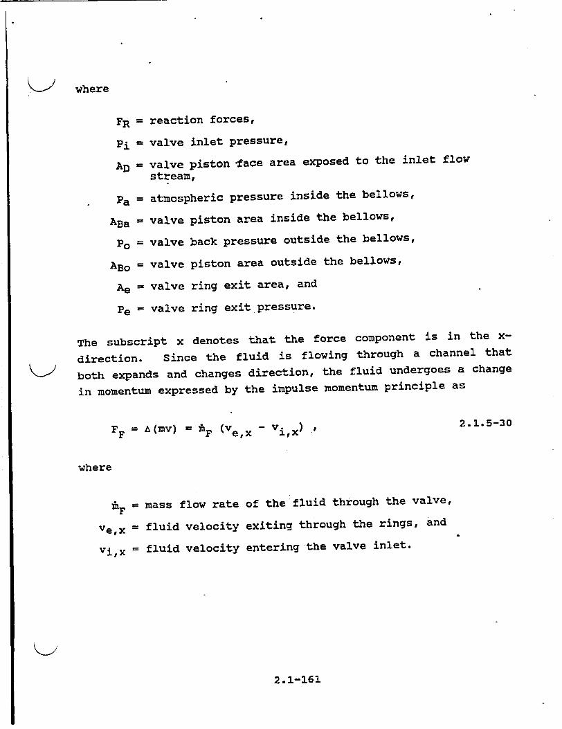
K-J where

FR = reaction forces,

pi = valve inlet pressure,

AD = valve piston face area exposed to the inlet flow stream,

Pa = atmospheric pressure inside the bellows,

ABa = valve piston area inside the bellows,

Po = valve back pressure outside the bellows,

ABo = valve piston area outside the bellows,

Ae = valve ring exit area, and

Pe = valve ring exit pressure.

The subscript x denotes that the force component is in the x

direction. Since the fluid is flowing through a channel that

both expands and changes direction, the fluid undergoes a change

in momentum expressed by the impulse momentum principle as

SA (MV)A (= fvn ) 2.1.5-30

F = F e,x - Vi,x

where

iF = mass flow rate of the fluid through the valve,

Ve,x = fluid velocity exiting through the rings, and

Vi,x = fluid velocity entering the valve inlet.

2.1-161

<21

Piston, rod assembly ,

Inlet 81= 0

Figure 2.1.5-10. Schematic of a Typical Relief.Valve in the Closed Position.

2.1-162

K-'

VV

Figures 2.1.5-11. and 2.1.5-12.

K

ABa)

Schematic of a Typical Relief Valve in the Partially and Fully Open Positions, respectively.

2.1-163

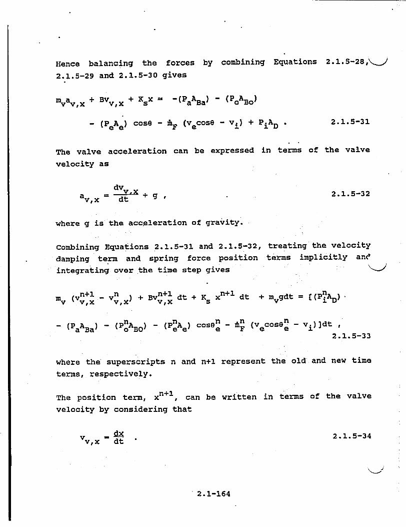
Hence balancing the forces by combining Equations 2.1.5-28,"\

2.1.5-29 and 2.1.5-30 gives

mvav x + BVv,x + %x -(PaABa) - (PoABo)

- (PeAe) cose - AF (vecosO- vi) + PiAD2.1.5-31

The valve acceleration can be expressed in terms of the valve

velocity as

av,x = dt + g I 2.1.5-32

where g is the acceleration of gravity.

Combining Equations 2.1.5-31 and 2.1.5-32, treating the velocity

damping term and spring force position terms implicitly ane

integrating over the time step gives

mv (' .-v ) + Bvn+l dt + xn+l dt + mvgdt =(P•AD)• V vvex v'x s ~ V

(vn n - Vc n v n (PaABa) o - (PABO) -o(Pe) x coooe - v Ft

2.1.5-33

where the superscripts n and n+l represent the old and new time

terms, respectively.

The position term, xn+l, can be written in terms of the valve

velocity by considering that

dx Vvx =d-t " 2.1.5-34

-I

1 2.1-164

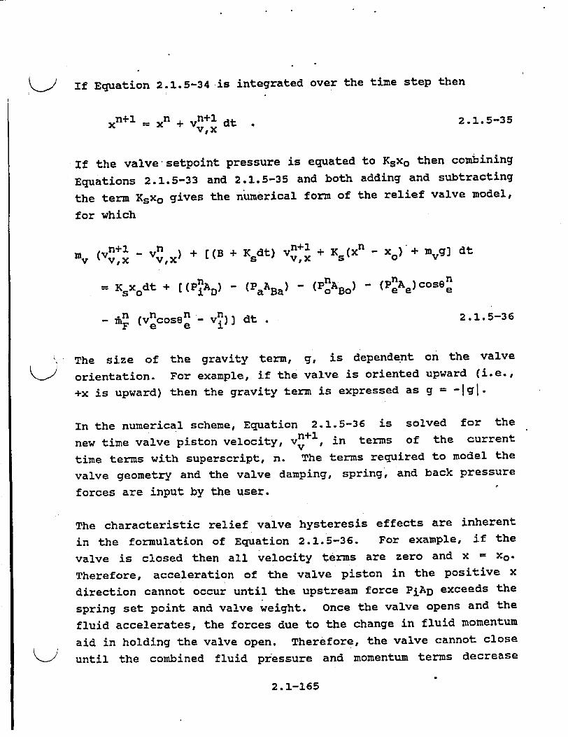
K> If Equation 2.1.5-34 is integrated over the time step then

n+1 n n+l

xn+1 = xn + vn1 dt . 2.1.5-35

If the valve setpoint pressure is equated to KsXo then combining

Equations 2.1.5-33 and 2.1.5-35 and both adding and subtracting

the term Ksxo gives the numerical form of the relief valve model,

for which

v n+1l n n+l vv'X --vý,' + [(B + Xsdt) V + Ks(Xn x0) + mvg] dt

K Vxdt + nP n A ( nA (x A [(B A K ) -S n

so 0'D a Ba 'o Bo' e (eecoee

.n n n n -m (v cos - v)] dt. 2.1.5-36

F (ese e I

SThe size of the gravity term, g, is dependent on the valve

orientation. For example, if the valve is oriented upward (i.e.,

+x is upward) then the gravity term is expressed as g = -Igl

In the numerical scheme, Equation 2.1.5-36 is solved for the n+l intrso h urn new time valve piston velocity, vv j in terms of the current

time terms with superscript, n. The terms required to model the

valve geometry and the valve damping, spring, and back pressure

forces are input by the user.

The characteristic relief valve hysteresis effects are inherent

in the formulation of Equation 2.1.5-36. For example, if the

valve is closed then all velocity terms are zero and x = xo.

Therefore, acceleration of the valve piston in the positive x

direction cannot occur until the upstream force PiAD exceeds the

spring set point and valve weight. Once the valve opens and the

fluid accelerates, the forces due to the change in fluid momentum

aid in holding the valve open. Therefore, the valve cannot close

until the combined fluid pressure and momentum terms decrease

2.1-165

below the set point forces. Hence, the desired hysteresis isKJ

incorporated in the model.

2.1.5.4. Accumulator Model

An accumulator model is included in RELAP5/MOD2-B&W that features

mechanistic relationships for the hydrodynamics, heat transfer

from the tank wall and water surface, condensation in the vapor

dome, and vaporization from the water surface to the vapor dome.

Hydrodynamic Model

An accumulator is modeled in RELAP5 as a lumped-parameter

component. This modeling was chosen for two reasons; the spatial

gradients in the accumulator tank are expected to be small, and

special treatment of the equation of state can be utilized.

The accumulator model and associated notations are shown in

Figure 2.1.5-13. The basic model assumptions are:

1. Heat transfer froim the accumulator walls and heat

and mass transfer from the liquid are modeled using

natural convection correlations assuming similarity

between heat and mass transfer from the liquid

surface.

2. The gas in the gas dome is modeled as a closed

expanding system composed of an ideal gas with

constant specific heat. The steam in the dome exists at a very low partial pressure and hence its

effect on the nitrogen state is neglected. However,

energy transport to the gas dome as a result of

vaporization/condensation is included.

3. Because of the high heat capacity and large mass of

water below the interface, the water is modeled a.

an isothermal system.

2.1-166

4. The model for liquid flow includes inertia, wall

friction, form loss and gravity effects.

Using these assumptions, the basic equations governing the

thermal-hydraulics of the tank and discharge line for

conservation of mass (nitrogen) can be written-as

"Mn = constant = pn Vn 2.1.5-37

where

"Mn and pn = gas mass and density, respectively, and

V = gas dome volume n

for conservation of energy.

Nitrogen

Mn aUn PD avv + 6D

where

u = nitrogen internal energy n PD = vapor dome pressure, and

QD = heat transfer rate to the gas dome.

wall

2.1.5-38 I

M C wall Vwall"aTwall w

at wall2.1.5-39

Rev. 2 8/92

2.1-167

K->

where K-)

Mwall = metal mass in the tank wall,

CVwall = metal specific heat,

Twall = mean metal temperature, and

Qwall = heat transfer rate to the wall.

For momentuma

pA (L v+_IV2) +AL at 2 ax Z.

2. 1.5-40

where

A = flow channel cross-sectional area,

v = velocity,

F = frictional loss coefficient, and

APz = elevation pressure differential.

For the gas state relationships

PDVv = MnRnTD 2.1.5-41

Un = Mn CvnTD T 2.1.5-42

aEquation 2.1.5-40 is the combined tank and discharge line momentum equations. The wall drag coefficient, F, is given as 1 / 2 Pwf LL/D ALV, ,where D = surge line diameter.

<2

2.1-168

K-I

and

* K> Using Equations 2.1.5-41 and 2.1.5-42, the nitrogen energy

equation (Equation 2.1.5-40), can be rewritten as

dT n PD vAL +QD 2.1.5-43

Differentiating Equation 2.1.5-41, eliminating the constant term

HnRn and substituting the result into Equation 2.1.5-43 yields

P 1 + k]Cývj + Vv d! = !Cvn_ 2.1.5-44

Equations 2.1.5-40, 2.1.5-43, and 2.1.5-44 comprise the system of

three differential equations used in the accumulator hydrodynamic

model. They are used to numerically advance TD, Vv, and PD in

time.

Heat Transfer to the Gas Dome

In the accumulator, energy transport by heat transfer is modeled

to the gas dome using a typical connective transport equation of

the form

Qi = hi Ai (Ti - Td) ' 2.1.5-45

where

subscript i = thermal transport interface,

hi = convective transport coefficient,

Ai = interface surface area, and

Ti - Td = interface to gas dome temperature difference.

2.1-169

Steami and nitrogen vapor

0 0 o

0 Volume VD Temperature TD

Wall heat "Pressure PD

0 0

0 0 0

Liquid water

Volume Vw Temperature Tw

h

Cross sectional area AL

LL

v -exhaust t line velocity

SP - system pressure

Figure 2.1.5-13. Typical Accumulator.

2.1-170

it should be noted that heat and mass transfer in the accumulator

surge line are neglected.

Two turbulent natural convection heat transfer models are used

and combined by superposition. First, heat transfer with the

cylindrical walls of the tank is considered using a turbulent

natural convection correlation9 6 for heat transfer within a

vertical cylinder with closed ends for which

kd hI = 0.1 d (Gr Pr) 2.1.5-46

2 TK

and

A1 7rDTK L 2.1.5-47

- where

hl = gas dome to cylinder heat transfer coefficient,

L = gas dome cylinder length,

6 = gas dome characteristic diameter,

kd = gas thermal conductivity,

1/2 DTK = integration interval normal to the surface of

the cylinder,

Gr = gas dome Grashof number, and

Pr - gas dome Prandtl number.

second, heat transfer with the disk shaped ends of the cylinder

is considered, where the top disk is the metal top of the tank

and the bottom disk is the liquid-gas interface. For this model

a turbulent natural convection correlation5 6 is used for heat

2.1-171

transfer between two horizontal disks separated vertically where, '_

for each disk,-

kd -1 L h= 0.15 d (Gr Pr) 3 2.1.5-48

2.1.5-492 - 4 A - 4

In the correlations given by Equations 2.'1.5-4-6 and 2.1.5-49 the

product of the Grashof and Prandtl numbers represents the

convective thermal circulation in the gas dome, where the Grashof

number represents the circulation and the Prandtl number

represents the thermal diffusion. Only the Grashof number is a

function of the gas dome dimensions and temperature difference

for which

god I Ti - Td 3

22.1.5-50

where

g = acceleration due to gravity,

Pd = gas isobaric coefficient of thermal expansion,

Ti - Td = magnitude of the interface, gas dome temperature difference,

Pi = gas kinematic viscosity, and

6 = characteristic overall diameter of the gas dome.

2. 1-172

and

Gr =

If the Prandtl number is written in terms of the gas dome thermal

diffusivity then

Pr = -P , 2.1.5-51

Pdad

where

Pd = gas density and

Od = thermal diffusivity.

The characteristic diameter is defined in terms of the typical

volume to surface area ratio as

4 V 6 _ A. , 2.1.5-52

where

Ai combined gas dome cylinder, disk top, and bottom surface areas.

Mass Transfer to the Gas Dome

When the accumulator is in its stagnant initial condition the gas

dome and liquid are in thermal equilibrium and the gas dome is at

essentially 100% humidity. However, as the accumulator blows

down, the gas dome expands and cools while the liquid remains

essentially isothermal. As a result there is simultaneous

vaporization at the liquid-gas interface and condensation in the

gas dome.

At the liquid-gas interface as vaporization occurs the vapor

diffuses across the temperature gradient into the gas dome.

Assuming that the process can be approximated by a quasi-steady

2.1-173

formulation, then for diffusion in a stagnant gas the mass,>

transfer for the process can be written as

Mvap = - Ai d• 2.1.5-53

Mvap = rate of vapor diffusion,

S= diffusion coefficient,

Ai = surface area of the liquid-gas interface, and

T__= vapor concentration gradient. dx

The concentration can be expressed in terms of partial pressure

such that

2.1.5-54Pv C d Pd 9g

where

C =.vapor concentration,

Pv = local vapor partial pressure, and

pg = vapor density (saturated vapor at Pv)

Hence at the dome pressure, the concentration gradient can be

written as

dC 1 dPvpg dx P d dx 2.1.5-55

2.1-174

where

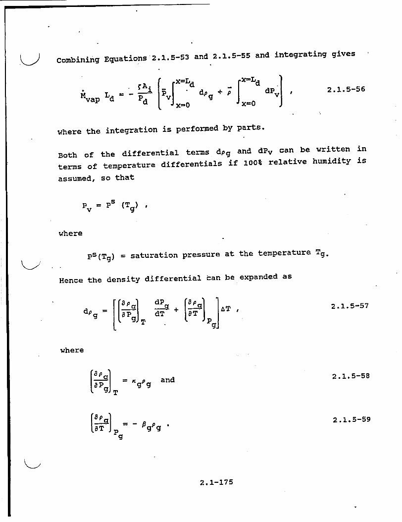
combining Equations 2.1.5-53 and 2.1.5-55 and integrating gives

Mvap Ld -d 2.1.5-5

where the integration is performed by parts.

Both of the differential terms dpg and dPv can be written in

terms of temperature differentials if 100% relative humidity is

assumed, so that

Pv = Ps (Tg)

where

PS(Tg) = saturation pressure at the temperature Tg.

Hence the density differential tan be expanded as

dPg= [+6 dT AT g gIg

2.1.5-57

where

[a- = p and

8PgJT g= gP *

(b]Pg P~

2.1.5-58

2.1.5-59

2.1-175

Combining Equations 2.1.5-57, 2.1.5-58, and 2.1-5759, anc substituting Clapeyron's equation for the dPs/dT term gives

dp P [cg[ __ _fg] dT ,2.1.5-60

where Clapeyron's equation is

dP = Tgf dT, 2.1.5-61

and where the term (hfg/TgVfg) is treated as a constant. Combining Equations 2.1.5-56, 2.1.5-60, and 2.1.5-61 the diffusion equation can be rewritten as

dvap f gg [g v - -+ -v- (Tf - Tw).

2.1.5-62

The dome average terms are evaluated at the dome average temperature, Tg = Td, and Tw is the tank top wall temperature.

Equation 2.1.5-62 can be made analogous to a convective equation by expressing the mass transfer coefficient as

h2s Ld' 2.1.5-63

h2s = mass transfer coefficient in a stagnant gas.

2.1-176

where

Then, by applying Reynold's analogy a turbulent natural

convection mass. transfer coefficient can be derived in terms of

the heat transfer coefficient, h 2 , from Equation 2.1.5-48 such

that

h 2 h2 L) ) 1/3 2.1.5-64

Equation 2.1.5-64 can then --be substituted in place of (C/L) in

Equation 2.1.5-63 such that

"kd *)j~ jPg Pg [~kg [TVý -fg

- rTT - TO

which gives the rate at which water vapor is transported into the

accumulator gas dome by turbuleht diffusion.

Since the energy transported to the gas dome by the vaporization

process must come from the liquid and since the energy per unit

mass required for vaporization is hfg, then the rate of energy

transport to the gas dome by vaporization is

6vap ' rvap(hfg) T = Mvap (h ) T 2.1.5-66

where rvap is the rate of vaporization at the liquid gas

interface.

In the gas dome, as the accumulator blows down, the gas cools and

condensation by turbulent diffusion occurs. The rate of

condensation may be approximated by assuming that the gas dome

2.1-177

remains at 100% humidity and considering simple humidity\

relationships. The humidity ratio can be written as

M NnP

WMn NnPD

where

14g, Mn = vapor, gas masses, respectively,

Ng, Nn = vapor, gas molecular weights, respectively, and

Pg = vapor partial pressure.

Taking the derivative of Equation 2.1.5-67 gives

2.1.5-67

dM ___PD

[M !! M dP

dt PD nNndt g dt 2.1.5-68

From Gibb's equation, the relationship between the vapor and liquid condensate in the dome is

dPD

dT-- f SPD,TE. 2.1.5-69

Substituting the relationship

dP dP dT dt dT dt 2.1.5-70

into Equation 2.1.5-69 and rearranging gives

Vf PD,TD dPD

V dt gP- T g'

hg gq l TD

T-V

- hf dTD

dt 2.1.5-71-D gpg,TD

2.1-178

V gPg, TD

(P D dTD S

ggTD= f

PD' TD

dt

dt

,<2

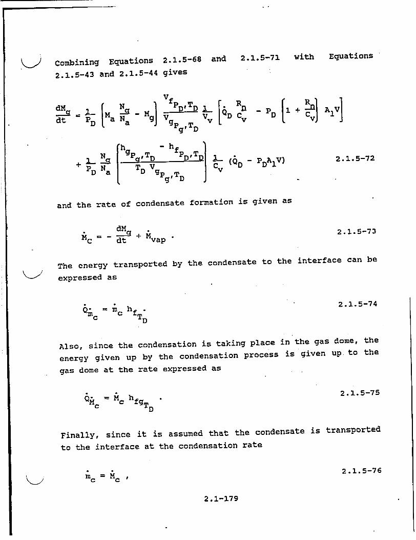
combining Equations 2.1.5-68 and

2.1.5-43 and 2.1.5-44 gives

with Equations

! !a Ma Na- M dt = D

2.1.5-72% h g -hfAlV)

and the rate of condensate formation is given as

dtq + a 2.1.5-73 c dt Mvap

The energy transported by the condensate to the interface can be

expressed as

Q; mchf . 2.1.5-74

TD

Also, since the condensation is taking place in the gas dome, the

energy given up by the condensation process is given up to the

gas dome at the rate expressed as

6 =A hfgTD 2.1.5-75

cD

Finally, since it is assumed that the condensate is transported

to the interface at the condensation rate

; C 2.1.5-76

K / mc MC

2.1-179

K-> 2.1.5-71

; [6 DRn -pD + A i_ Cv -] + v I

and the net energy given up to the gas dome by the condensation,,"

process can be expressed as

6. 6 Qc - Q;c =(chfgTD - hf ) " 2.1.5-77

Energy Transported to the Gas Dome by Combined Heat and Mass Transfer

The total energy transported to the gas dome can be rewritten by combining Equations 2.1.5-45, 2.1.5-46, 2.1.5-48, 2.1.5-66, and

2.1.5-77 and summing to give

6D = (h1A 1 + h2A2 ) (Tw Td) + h 2 A2 (Tf Td) + Mvap hgTf

+ mc (hfgT - hf d 2.1.5-78

Numerical Imnlementation

The numerical scheme used for the accumulator model includes special features for coupling the solution scheme to the main

code in such a way that it is time step independent. This scheme, as in RELAP5, is semi-implicit and special considerations

are employed to preserve the nitrogen energy and mass.

The numerical scheme uses finite difference techniques to solve

the differential equations. The momentum equation is formulated

2.1-180

by integrating Equation 2.1.5-40 over space and writing the time

variation in difference form as

~pf(Lf + Lf)A +FPfAt+ PgL +g)j )Fgt vl

+t + fL

(pn+l - _ n+l t+APA p + L (%

+ Pg (tgL+] v - CONVF - CONVG t

+ gT A fL 2.1.5-79

h n+l = pressure downstream from the accumulator junction. p

The inertia term is represented by

2.1.5-80pf( Lf + jL

where Lf , Lf , , and L are the lengths of the liquid and LL' LTK' g' LT

gas in the surge line and tank, respectively. These terms are

computed at each time step and hence vary explicitly with time

having the effect that as the accumulator blows down the inertia

term changes from a liquid dominant to a vapor dominant term. The

liquid and gas friction terms, respectively, are'formulated as

a Lf L Lf F 2 DL LLL fL

2.1.5-81

Rev. 2 8/922.1-181

IL

where

for the liquid, and

Fg=9 ~( I!L+ ~LgIvn 2 D L LL j

2.1.5-82

for the vapor. Friction is neglected in the tank and the line

friction factor is assumed to be the constant turbulent-turbulent

Darcy friction factor given as

S= [1.74 - 2 Log D

DL]2.1.5-83

The loss factor term, KL, is assumed to be distributed over the surge line length, LL. The term DL is the surge line hydraulic diameter and c is the surge line wall roughness. The elevation head term, AP z, is formulated as

gazTK (PfLfTK + IP Lg gAz (PfLf + gL)

LL

2.1.5-84 where AzTK and AzL are the tank and surge line elevation changes,

respectively, and g is the gravitational acceleration. The liquid and vapor momentum flux terms, CONVF and CONVG,

respectively are formulated as

( 2vf - v ) 2.1.5-85ifthee = is lqi i t , t vn

if there is liquid in the tank,

CONVF = 0.0 2.1.5-86

Rev. 2 2.1-182 8/92

APz = -

<2I

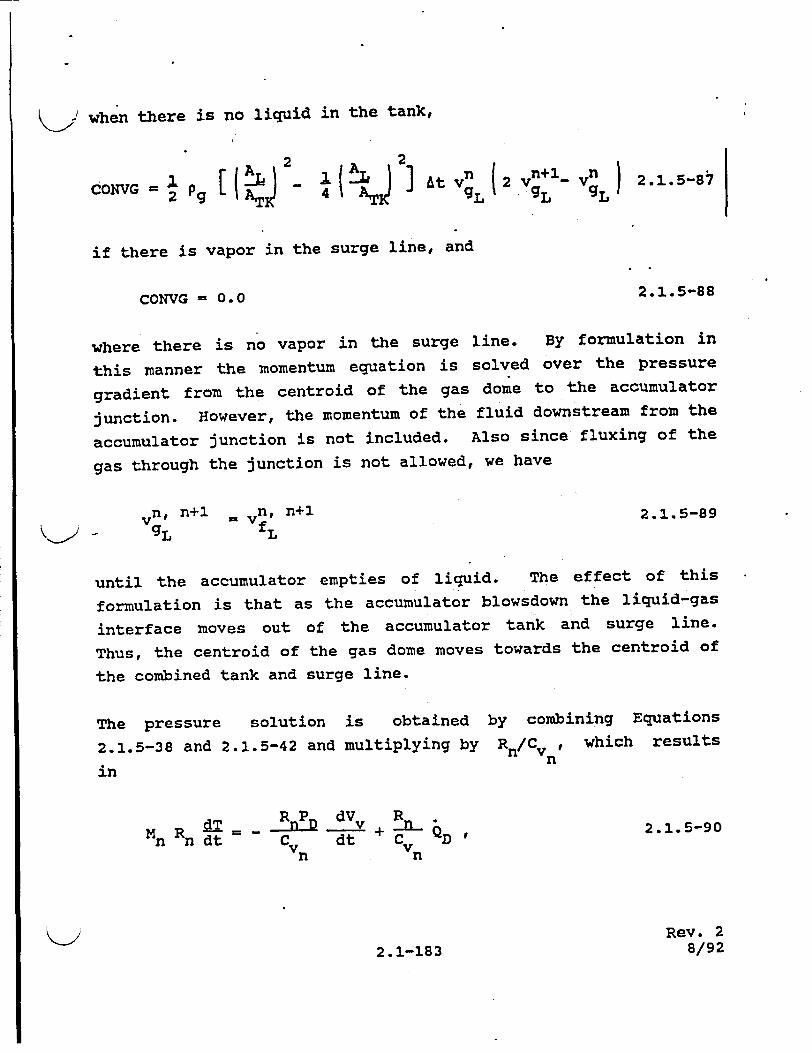
when there is no liquid in the tank,

Atv~ (2 n~-~~~ 2.1.5-8 dONVG = 2 Pg 94 gL (L gL

if there is vapor in the surge line, and

CONVG = 0.0 2.1.5-88

where there is no vapor in the surge line. By formulation in

this manner the momentum equation is solved over the pressure

gradient from the centroid of the gas dome to the accumulator

junction. However, the momentum of the fluid downstream from the

accumulator junction is not included. Also since fluxing of the

gas through the junction is not allowed, we have

v n, n+l v nv' n+l 2.1.5-89

until the accumulator empties of liquid. The effect of this

formulation is that as the accumulator blowsdown the liquid-gas

interface moves out of the accumulator tank and surge line.

Thus, the centroid of the gas dome moves towards the centroid of

the combined tank and surge line.

The pressure solution is obtained by combining Equations

2.1.5-38 and 2.1.5-42 and multiplying by Rn/Cv n which results in

RP dV

'n Rn d•tCt dtv D+ 2.1.5-90

Rev. 2

2.1-183 8/92

where QD is given by Equation 2A..5-78.

2.1.5-90 are then combined resulting in

ndVv dP R PD I + C -vn + Vv dt Cvrin QD

Since the liquid is incompressible

Equations 2.1.5-41 and •

2.1.5-91

dVv dVf at - - t = ALvjf 2.1.5-92

and substitution in Equation 2.1.5-91' and expanding in

nonconservative finite difference form gives

P n 1 l+ 1o vn+1 + Vn Pn+I DI C I A tVf + vVI D I VJn

- p n )n at CvnD

2.1.5-93

The energy equation may then be solved directly for the new time

gas temperature by combining Equations 2.1.5-41, 2'.1.5-44, 2.1.5

91, and integrating, which gives

CV n =+T e LVV Tn+l n lj n+ t v.

D D 2.1.5-94

2.1-184