Public Works and Government Services Canada Travaux publics et Services gouvernementaux Canada

TRANSLATION BUREAU

MULTILINGUAL TRANSLATION DIRECTORATE

BUREAU DE LA TRADUCTION DIRECTION DE LA TRADUCTION MULTILINGUE

Request No.

Language Originator File No.

Date

1694120

Swedish/PC

No.de la demande Langue Référence du demandeur Date

Translation begins on next page.

CHALMERS

Flare testing using the SOF method at Borealis Polyethylene in the summer of 2000

Johan Mellqvist

Chalmers University of Technology

Götِeborg, 3 October 2001

Acknowledgments

I was assisted in this project by Christina Birath (Rintekno), who helped with the calculations and measurements, and by Magnus Ekströmِ (IVL), who helped carry out the measurements.

2

Summary

A study of flaring efficiency at the Borealis low-pressure plant in Stenungsund was conducted using a new patented method called Solar Occultation Flux (SOF), in combination with a new type of direct measurement of flow rate and ethylene concentration in the flare stack. The SOF method is based on the measurement of hydrocarbon concentrations over a cross-section of the emission plume. Multiplied by wind speed, this gives the flux of gas through the cross-section, i.e., the source emission in kg·s-1. In the measurements, the sun was used as the light source. An infrared FTIR spectrometer linked to a sun tracker was placed on top of a van that was driven in such a way that the sunlight shone through a cross-section of the plume being measured. From the size of the molecular fingerprints in the infrared solar spectra, the concentration of ethylene and other constituents can be calculated. The results show that the flare we studied has a good combustion efficiency of about 98% at high loads (>1100 kg·h -1), but that at low loads, which are the normal operating conditions most of the time, it has a significantly lower efficiency (50-90%). Emissions thus appear to vary between 20 and 50 kg/h irrespective of load – a result that is consistent with other long-term FTIR measurements taken outside the plant. Similar emission results were also obtained during the course of the project from a newly installed flare, so that the problem does not appear to be specific to the flare that we studied. From the measurements in this study it can be concluded that a major contributing factor in the poor efficiency is an overdose of steam at low operating loads, as a result of trying to avoid soot formation by optimizing flare combustion at high loads. The problem can presumably be solved by introducing some form of dynamic steam metering linked to combustion load, or by eliminating the presence of ethylene at low operating loads. The direct flare stack measurements show that the heating value is generally low, and that theoretically we could therefore expect poorer efficiency levels. It was not possible to demonstrate this unambiguously in the present study, however, since the steam and ethylene levels were generally covariant. Only in a few cases did we find a low efficiency at low ethylene concentration, independent of steam quantity.

3

1. INTRODUCTION................................................................................................................................................. 5

1.1 FLARES............................................................................................................................................................ 5

2. MEASUREMENT METHOD.............................................................................................................................. 7

2.1 THE SOLAR OCCULTATION FLUX (SOF) METHOD.............................................................................................. 7 2.2 DIRECT MEASUREMENT IN THE FLARE STACK..................................................................................................... 11

3. MEASUREMENTS............................................................................................................................................. 12

4. RESULTS............................................................................................................................................................. 16

5. DISCUSSION....................................................................................................................................................... 19

5.1 EMISSIONS............................................................................................................................................................ 19 5.2 EFFICIENCY...................................................................................................................................................... 21 5.3 VIDEOTAPING OF THE FLARE.................................................................................................................................. 25

5. CONCLUSIONS.................................................................................................................................................. 26

6. REFERENCES.................................................................................................................................................... 28

4

1. Introduction During 1998 and 1999 automatic concentration measurements were taken outside the Borealis Polyethylene plant in Stenungsund using an infrared remote sensing system [1-5]. It was found that the average ethylene load calculated over a period of six months was relatively high when it was blown from two flares burning surplus gas from a catalytic process forِ the production of polyethylene. The results of a diffusion model, in combination with the concentration measurements, indicated that the flares emit roughly the same amount (or more) than the previously known emissions combined (≈300 tonnes ethylene/year). This had not previously been known, and it had instead been assumed that the flares did not emit any significant amount of hydrocarbons. In this project we have now conducted further tests on the same flares in order to better understand the cause of these emissions and to quantify the flares’ efficiency, whether the emissions are the result of flare gases passing the pilot flame without igniting or the flare is burning at low efficiency because of its construction. Measurements were taken using a new method (SOF) patented by us, thanks to which it was possible to measure the flares' instantaneous emission (kg/h). In addition, we carried out direct measurements in the flare gas stream in one of the flares (LP1) upstream of combustion, combined with trace gas emissions, from which it was possible to calculate the quantity of ethylene flared (kg/h) as well as the flare gas flow rate (m3/h). During the measurement period the LP2 flare was operating at low capacity because a new plant (Borstar) was just then in the process of being set up, and the LP2 plant was not running at full capacity. 1.1 FLARES Flaring is a process used to burn components, mostly hydrocarbons, of waste gases from industrial operations. In combustion, the gaseous hydrocarbons react with atmospheric oxygen to form carbon dioxide and water. Presented below is the combustion reaction for ethylene (without soot).

C2H4 + 2O2 ÷ 2 CO + 2H2O (+O2) ÷ 2CO2 + 2H2O

There are two types of flares, ground flares and elevated flares, of which the latter are more common. In elevated flares, a waste gas stream is fed through a stack anywhere from 10 to over 100 metres tall and is combusted at the tip of the stack. In ground flares, combustion takes place, as the name suggests, at ground level. They may consist of conventional burners with no enclosures or may be built into steel enclosures. The typical flare system consists of (1) a gas collection header and piping for collecting gases from processing units, (2) a knockout drum to remove and store condensables and entrained liquids, (3) a proprietary seal, water seal, or purge gas supply to prevent flash-back, (4) a burner unit and a flare stack, (5) gas pilots and an ignition system and, if required, (6) a provision for steam injection or forced air for smokeless flaring.

5

Complete combustion requires sufficient air and proper mixing of air and flare gas. Combustion of paraffins above methane, olefins and aromatics causes smoke. Steam injection (steam-assisted flares) or blowing air (air-assisted flares) at the flare tip are used to improve the supply of air and achieve efficient air/fuel mixing, thereby promoting smokeless flaring. Flares are normally designed to dispose of low-volume continuous hydrocarbon emissions that for environmental reasons can not be vented directly into the atmosphere, but also to handle large quantities of waste gases that may be intermittently generated during plant emergencies or temporary shutdowns. Soot formation tends to increase at higher carbon-to-hydrogen (C-to-H) ratios. All hydrocarbons above methane, i. e., those with a C-to-H ratio of greater than 0.33, tend to soot. Flare gas composition is a critical factor in determining the amount of steam necessary for smokeless flaring. Emissions from flaring include carbon particles (soot), unburned hydrocarbons, carbon monoxide (CO) and other partially burned hydrocarbons, as well as NOx. The quantities of hydrocarbon emissions generated relate to the degree of combustion, which in turn depends on the gas velocity, the degree of fuel-air mixing, the flame temperature and the heating value of the flare gases. Flare efficiency is generally very difficult to measure on actual flares. Most studies have therefore been done on model flares (1/4 or 1/2 scale) or at laboratory scale, and these have shown efficiencies varying from 55% to 99%, depending on stability and flare type [6]. A few measurements on actual flares (solution gas flares without pilot flame and refinery flares) have also been made [7, 8], with combustion efficiencies varying between 62 and 98%. In a recently completed study on flares [9], in which CO was the primary flare gas, the so-called long path FTIR was used in combination with tracer gas emissions. Combustion efficiencies of about 90% were obtained, which was significantly higher than the model studies (CO has a low thermal value). None of the above measurements, however, were conducted on the type of flares used at the polyethylene plant in Stenungsund. Before it was discovered that these flares were not performing satisfactorily, their efficiency was estimated to be above 99% according to the EPA standard. Each of the flares is connected to a low-pressure plant (LP1 and LP2). The latter flare is also used by the new Borstar plant (PE3). The LP2 flare was replaced in the summer of 2000 by a new, larger flare in conjunction with the construction of PE3 for the production of bimodal polyethylene. Relief valve lines are connected to the flares, as are various more or less continuous streams of process hydrocarbons, especially ethylene. Both flares are steam assisted, i.e., steam is injected into the flare tip to minimize soot formation. Steam injection to both flares is regulated manually. The LP1 flare is 40 metres high and has a combustion capacity of 150 tonnes per hour. The LP2/PE3 flare is 70 metres higِh and has a maximum capacity of tonnes per hour (ethylene). At the base of each flare stack is a knockout drum for separating out any entrained liquid, condensed gas or polymers. The flares have no water seal but are equipped with a gas seal just below the flare tip. In addition, a stream of nitrogen gas is continuously flushed into the flare system and out again through the flare stack to prevent air ingress.

6

The fuel for the pilot burners is usually pure ethylene. The gas streams sent to the flares at the polyethylene plant normally contain only a small amount of hydrocarbons. The gas comes largely from waste-gas tanks where the polyethylene product is purged with nitrogen to remove the remaining unreacted ethylene or comonomers. Gas with a higher hydrocarbon content is fed from the reactors’ product system to the flare system as the product is discharged. The discharge frequency depends on the production rate. The gas that is flared with each product discharge arrives in pulses of large volume within a short period of time. Part of the vent gas from one of the reactors at LP1 is also sent to flare. From the gas purification at the HP plant, which does not have its own flare, a butene-rich stream and an ethane-rich stream are conveyed to the LP1 flare system. The HP gas streams are relatively small. In addition to the gases from the waste-gas tanks and product discharges, continuous waste gas streams from the Borstar plant containing large amounts of propane, butene and ethylene are fed to LP2's flare. Because the flare gas normally contains a small hydrocarbon fraction and a large inert nitrogen fraction, the heating value of the gas is low, which decreases combustion efficiency. Large swings in flow rate and content also affect combustion. The steam injection is manually controlled to obtain a smokeless flame with the richer flare gas from product discharges or other sources. Often this results in an excess of steam being added in relation to the hydrocarbon content of the gases. Too much steam can reduce the degree of combustion efficiency and causes noise. If the surplus of steam is very large, the flame will become unstable. 2. Measurement method 2.1 The SOF (Solar Occultation Flux) method In this study we have used a new method patented by us, the SOF (Solar Occultation Flux) method, to quantify instantaneous emissions from the flares. The method is based on an infrared spectrometer connected to a sun tracker, position determined by GPS, and wind measurement. The SOF instrument is mounted on a van. The instrument records infrared spectra from the sun as it shines through the emission plume under study. The infrared spectra contain information about the quantity of fugitive gas emission (ethylene) along the light path (total column). They also contain information about a number of other substances found in the atmosphere. The absorption from these other species, however, interfere with our measurement, and are eliminated by dividing all the spectra by a reference spectrum measured just outside the plume. After a traverse of the plume, the total column measurements can be added together and multiplied by the plume's length measured by GPS to obtain the total quantity of fugitive gas over the plume's cross-section. The emission flux through the plume's cross-section is then found by multiplying by the measured wind speed. This method of obtaining the flux is identical to what is done in the laser-based DIAL technique [8]. Measurement by SOF is very sensitive, and studies have shown that it is possible to detect sources down to a few kg·h-1 at a distance of 50-100 m. Figure 1 shows the measurement principle, Figure 2 the measuring instrument itself, and Figure 3 an absorption spectrum (fingerprint) for ethylene together with a fitted laboratory spectrum.

7

In the SOF estimates we corrected for the fact that we did not always traverse the plume at right angles and for the sun's narrow angle of incidence. The quantity of fugitive gas emission was estimated by a mathematical comparison of the magnitude of the measured absorption with calibration spectra obtained from a calibration database called Hitran [10, 11], which is considered to be the best for IR absorption measurements. The uncertainty in the mass flow measurements is due in part to the error in the concentration measurements arising from the relatively high detection limit and in part to the error in determining the concentration-weighted mean wind. For the measurements at Borealis Polyethylene wind speed was determined using an anemometer placed on an elevated mast on the highest tower at the site (HP-PEX) (about 70 m). One-minute mean values were used for the SOF calculations. Figure 4 illustrates a traverse 200 m NE of the flares. The emission plumes from the flares at the 2nd (left) and 1st (right) low-pressure plant (LP) can be seen in the figure, corresponding to instantaneous ethylene emissions of about 35 och 63 kg·h-1 respectively.

Solljus => Sunlight Utsläppsplym => Emission plume (tvärsnitt) => (cross-section) Solföljare => Sun tracker FTIR => FTIR Förflyttningsriktning => Direction of motion Figure 1. Measurement principle for SOF. Infrared spectra from the sun are measured by an FTIR connected to a sun tracker. The instrument is mounted on a vehicle that is driven in such a way that the light beam traverses a cross-section of the plume. The measurements are integrated to obtain the quantity of hydrocarbons across the plume's cross-section. This is multiplied by the mean wind speed to derive the mass flux.

8

FTIR => FTIR Solföljare => Sun tracker Figure 2. The SOF apparatus as used on a pickup truck. The system consists of a Bruker spectrometer (0.5 cm-1 resolution), a sun tracker and transfer optics.

Figure 3. An absorption spectrum for ethylene corresponding to a total column of 21 mg/m3 over 1 m. The spectrum was measured 120 m downwind of an ethylene oxide production area. Calibration spectra (references) for ethylene, water and ammonia were fitted to the measured spectrum by the multivariate CLS technique. The difference between the spectra is shown as the residual and corresponds to an uncertainty of about 0.5 mg/m3.

9

left vertical axis Ethylene column (ppm over 1 m) right vertical axis Cumul. ethylene emission, kg h-1 horizontal axis Crosswind distance, m Eten-Kolumn => Ethylene column Ackumulerad emission => Cumulative emission LT2 => LP2 LT1 => LT1 Figure 4. SOF measurement of ethylene on 23/8/2000 along a gravel road about 200 metres northeast of the flares. The figure shows the gas column measured across the wind and the area under the column integrated along the direction of travel, corresponding to the cumulative emission. The emission plumes from the flares at both LP1 (right) and LP2 (left) can be seen in the figure, corresponding to instantaneous ethylene emissions of about 35 and 63 kg·h-1 respectively.

10

2.2 Direct measurements in the flare stack In order to calculate flare efficiency it is necessary to know the quantity of outgoing gas and to measure the emission after combustion. A new method for measuring flux was therefore developed in which a tracer gas (N2O) was injected 100 m upstream in the flare stack and then measured using an FTIR system designed by us, together with the outgoing ethylene content. This in situ measurement system was installed in a shed, see title page, about 60 m from the LP1 flare. The flare gas was pumped continuously through quarter-inch tubing to a 2.5 cm long measuring cell in which the ethylene and N2O content were determined with an FTIR spectrometer at one-minute intervals. Figure 5 is a schematic of the in situ measurement of flare gas composition and flow rate. Figure 6 shows the mass flux of ethylene and the total volumetric flow calculated for August 8 from the direct ethylene and tracer gas measurements.

SOF mätning av emission efter förbränning => Post-combustion emission measurement by SOF Fackelstam => Flare stack FTIR analys av eten och N2O => FTIR analysis of ethylene and N2O Figure 5. Nitrous oxide was injected as a tracer gas 100 m upstream in the flare stack. The ethylene and N2O concentration in the flare gas was then measured by FTIR. A low N2O concentration indicated a high flare gas flow and vice versa.

11

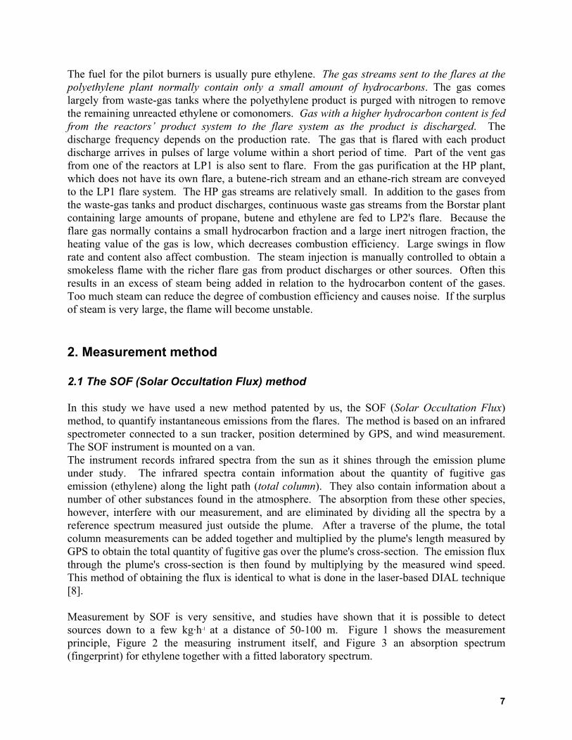
left vertical axis Total gas flow through the flare, Nm3h-1 right vertical axis Mass flow of ethylene through the flare, kg h-1 horizontal axis Time Totalt volymflöde => Total volumetric flow rate Eten massflöde => Ethylene mass rate Figure 6. Volume flow and mass flow measured August 8 in the flare stack from LP1. Flow measurements were made by injecting a constant quantity of nitrous oxide (1.18 kg/h) into the flare stack and subsequently measuring the nitrous oxide concentration downstream. Ethylene was also measured in order to calculate the quantity of ethylene flared. Note the large time variability. 3. Measurements Table 1 below gives the measurements taken during the course of the project. For various reasons only the data from August 9, 22 and 23 were used for the quantitative analysis of combustion efficiency. The measurements taken on the other days, however, show that the flares generally appear to emit ethylene at a rate varying between 10 and 150 kg·h -1. Figure 7 shows the experimental matrix to which these measurements correspond in ethylene flow and volume fraction. To reduce the analytical error, flare gas data was selected in which the variability over a 3-minute period was not too great (±50%). Figures 8, 9 and 10 show examples of SOF measurements from August 8 and 9. Figures 8 and 9 show a series of measurements from east to west (right to left) taken on August 9 a few hundred metres north of the plant. The expected positions of various plumes are also indicated in the figure. Figure 10 shows a measurement series along a gravel road northeast of the flares. The red dots indicate where high columns were measured and vice versa.

12

Table 1. The measurements carried out on the LP1 and LP2 flares. Wind speed atop the HP PEX plant was about 4-7 m/s throughout the measurement period. Date Time Wind direction Measurement site

2000-07-25 15:21-18:28 NW-W Industrial park

2000-08-07* 11:15-17:32 SW-W Italienbarackväg (N of the plant)

2000-08-08* 11:01-15:41 W Footpath (N of the plant)

2000-08-09 10:37-16 S Stripplekärrsvägen, Sandtagsväg

2000-08-18 12:30-16:17 S-SW Stenbrottsväg (N of the plant)

2000-08-21 13:18-17:30 S-SW Stenbrottsväg (N of the plant)

2000-08-22 13:41-16:30 SW-W Italienbarackväg (N of the plant)

2000-08-23 10:40-16:30 SW-W Italienbarackväg (N of the plant)

2000-08-25 10:40-16:30 NW-W Industrial park

2000-08-28 10:40-17:30 SE Stripplekärrsvägen

2000-09-04 10:40-17:00 N-NW-W Industrial park

2000-09-05 10:40-17:30 SW Stenbrottsväg (N of the plant)

2000-09-11 10:40-17:30 N-NW-W Industrial park

* Direct measurement system in the flare stack not functioning

left vertical axis Flow, m3h-1 horizontal axis Ethylene concentration, % Figure 7. Experimental matrix for the measurements on August 9, 22 and 23. Because of insufficient ethylene it was difficult to obtain measurements with a high ethylene content.

13

left vertical axis Ethylene column (ppm over 1 m) right vertical axis Cumul. ethylene emission, kg h-1 horizontal axis Crosswind distance, m Eten-Kolumn => Ethylene column Ackumulerad emission => Cumulative emission färdriktning => Direction of travel Plym LT1 / LT2 fackla => Plume LP1 / LP2 flare Plym HT fabrik => Plume HP plant

Figure 8. Measurement example from August 9 at Stenbrottsväg. The measured ethylene gas column is shown, together with the accumulated emission along the measurement path (east-west). The estimated positions of the plumes for the LP1 and LP2 flares and for the high-pressure plant are marked.

Figure 9. Measurement situation on 9 August 2000. Wind direction for the HP, LP1 and LP2 plumes are shown. SOF measurement positions and the measured gas columns (red high values, blue low). The expected plume lengths for the HP, LP1 and LP2 flares are shown as light green, dotted black and dark green lines respectively.

14

LT1 fackla => LP1 flare Figure 10. SOF measurements along a gravel track on 8/8. The blue to red scale corresponds to an ethylene gas column of 0-270 mg/m3 over 1 m. The emissions measured foِr the LP1 flare were 132± 68 kg/h. Flare load varied between 200 and 2000 kg h-1 with an ethylene content of 5-15% and a steam:ethylene ratio between 1 and 10.

15

4. Results Figures 11 to 16 show SOF measurements together with flare gas measurements of ethylene concentration, flow rate and quantity flared. The figures and their captions will be allowed to speak for themselves; the data will be discussed in section 5.

Figure 11. FTIR measurements in the LP 1 flare (in situ FTIR) and LP1 emission measurements by SOF for August 9 (Sandtagsväg). The flare burned well here during discharge. Otherwise the flare was transparent and "shimmered" with a faint steam plume.

16

left vertical axis Ethylene emission, kg/h right vertical axis Quantity of ethylene flared, kg/h horizontal axis Time Etenutsläpp => Ethylene released Facklad mängd => Quantity flared Figure 12. FTIR measurements in the LP 1 flare (in situ FTIR) and LP1 emission measurements by SOF for August 22 (Italienbarackväg). The flare burned well here during discharge, with a yellow, not quite smoky flame. Otherwise the flare was transparent with a faint steam plume.

axes as in Figure 12 Uppmätt emission SOF => Emission measured by SOF Facklad mängd (In situ) => Quantity flared (in situ) Figure 13. FTIR measurements in the LP 1 flare (in situ FTIR) and LP1 emission measurements by SOF for August 23 (Italienbarackväg). The flare seldom burned with a visible flame even during product discharge. Before 12:30 70% went from reactor 11 to flare, thereafter 40%.

17

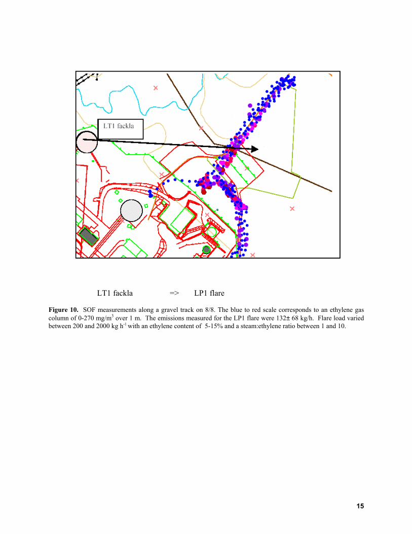
axes as in Figure 12 Etenutsläpp => Ethylene released Facklad mängd Eten kg/h => Quantity of ethylene flared kg/h Figure 14. FTIR measurements in the LP 1 flare (in situ FTIR) and LP1 emission measurements by SOF for August 28 (Stripplekärrsvägen). A problem with these measurements is the overlap between the LP1 and LP2 flares. The LP2 reactor, however, was taken out of service at 11:00 following a number of blow-offs between 10:00 and 11:00. Because of the uncertainty with the LP2 flare, the results were not incorporated in our further analysis.

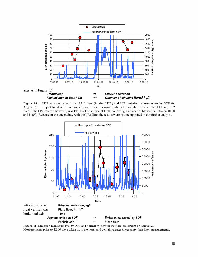
left vertical axis Ethylene emission, kg/h right vertical axis Flare flow, Nm3h-1 horizontal axis Time Uppmätt emission SOF => Emission measured by SOF Fackelflöde => Flare flow Figure 15. Emission measurements by SOF and normal m3 flow in the flare gas stream on August 23. Measurements prior to 12:00 were taken from the north and contain greater uncertainty than later measurements.

18

left vertical axis Ethylene emission, kg/h right vertical axis Ethylene concentration in the flare gas, % horizontal axis Time Uppmätt emission SOF => Emission measured by SOF Fackelflöde => Flare flow

Figure 16. Emission measurements by SOF and ethylene concentration in the flare gas stream on August 23. Measurements prior to 12:00 were taken from the north and contain greater uncertainty than later measurements. 5. Discussion Data from figures 11 to 16 were used to investigate which parameters covaried. Efficiency was calculated as the ratio of the emission measured by SOF to the flared quantity directly measured by the FTIR system. Because of the large time variability in the quantity of ethylene flared and the necessity of correcting for the time differences between the two measurements (SOF and FTIR) we did not include in our efficiency analysis process data in which there was too large a time variation (±1 min). 5.1 Emissions In the following three figures (17, 18 och 19) the measured emissions have been plotted against flare gas flow, ethylene concentration in the flare gas, and flared quantity. The highest emission levels are seen at low ethylene levels, low flow rates and low flared quantities. In Figure 19 the limits for various efficiency levels are also marked. The efficiency is 95-98% for the highest flared quantities (>1200 kg/h) but at lower values (<400 kg/h) it is significantly more variable and generally lower. The reason for this is discussed in section 5.2.

19

left vertical axis Ethylene emission, kg h-1 horizontal axis Flow rate, m3h-1

Figure 17. Emission as a function of total flow (Nm3/h) for August 9, 22 and 23. Uncertainty in the emission measurements is shown along the y-axis and variability in the flow over 3 minutes is shown along the x-axis.

left vertical axis Ethylene emission, kg/h horizontal axis Ethylene concentration, %

Figure 18. Emission as a function of flared quantity for August 9, 22 and 23. Variability in ethylene concentration over 3 minutes is shown along the x-axis, and a 30% uncertainty along the y-axis.

20

left vertical axis Ethylene emission, kg h-1 horizontal axis Quantity of ethylene flared, kg h-1

Figure 19. Emission as a function of flared quantity for August 9, 22 and 23. Limits are marked for 98%, 95% and 90% combustion efficiency. Variability in flared quantity over 3 minutes is shown along the x-axis, and a 30% uncertainty along the y-axis. 5.2 Efficiency In the following six figures, data has been twisted and turned in order to get at the source of the poor efficiencies we have sometimes observed. This is not easy, given the number of covariant parameters in these measurements. The database is also relatively small. Figures 20 to 22 show combustion efficiency in flare 1 as a function of flow rate, ethylene concentration and quantity flared. Each figure shows additional information for data obtained at low flow rates, ethylene levels or high steam to ethylene ratios (>4). Figure 21 also indicates the measurement dates. It can be seen in all three figures that there is often a high steam to ethylene ratio at low efficiency levels. The same is true, however, when flow and ethylene concentration are both low. Figure 23 shows combustion efficiency as a function of steam:ethylene ratio, and a clear correlation can be seen. Low flow rates and ethylene levels are also shown, and a negative correlation can be seen between combutstion efficiency and the steam to ethylene ratio. Low flow rates and concentrations are marked, and are seen at both high and low steam:ethylene ratios. In Figure 24, heating value is plotted against flare gas velocity in the form of ethylene concentration as a function of flare gas flow. In the figure, datapoints with an efficiency of greater than 97% are marked, together with data in the 90-97% efficiency interval. It can be seen that points with a 97% efficiency are all found at ethylene concentrations above 8% and flow rates above 5000 m3/h.

21

left vertical axis Efficiency, % horizontal axis Flow, m3/h Alla data => All data etenhalt<12% => Ethylene concentration < 12% Hög relativ ånga >4 => High steam to ethylene ratio, > 4:1

Figure 20. Efficiency as a function of total flow rate (normal m3). Low ethylene concentration and high steam:ethylene ratio (>4) are shown as small white squares and large hollow circles respectively.

left vertical axis Efficiency, % horizontal axis Ethylene concentration, % 08-aug (synlig låga) => 08 Aug (visible flame) 22-aug (synlig låga) => 22 Aug (visible flame) 23-aug (Rykande fackla) => 23 Aug (smoky flare) flöde<4000 m3/h => flow < 4000 m3/h "Hög rel ånga" => high steam:ethylene ratio Figure 21. Efficiency as a function of ethylene content by measurement date. Low flow rates and high steam to ethylene ratios (>4) are shown as small white diamonds and large circles respectively.

22

left vertical axis Efficiency, % horizontal axis Flared quantity, kg/h Alla data => All data Halt<12% => Concentration < 12% flöde < 4000 => Flow < 4000 Rel ånga >4 => Steam to ethylene ratio > 4:1

Figure 22. Combustion efficiency as a function of quantity flared. Low concentration, low flow rate and high steam:ethylene ratio (>4) are shown as small white triangles, hollow circles and large hollow squares respectively.

left vertical axis Efficiency, % horizontal axis kg steam / kg ethylene Verkningsgrad => Efficiency etenhalt < 12% => Ethylene concentration < 12% Flöde < 4000 m3/timme => Flow < 4000m3/h Poly. (Verkningsgrad) => Poly. (Efficiency) Figure 23. Efficiency as a function of the steam:ethylene mass ratio. Datapoints with a relatively low concentration are shown as small white squares, and points with low flow are circled. The data are from August 9, 22 and 23.

23

left vertical axis Ethylene concentration, % horizontal axis Flow, m3/h (velocity) Verkningsgrad 90-97% => Efficiency 90-97% Verkningsgrad> 97% => Efficiency > 97% Verkningsgrad<90% => Efficiency < 90% Relativ ånga/eten >2.5 => Steam:ethylene > 2.5:1

Figure 24. Heating value as a function of exit velocity in relative units. Datapoints with a high steam:ethylene ratio (>2.5) are marked with a small white diamond.

24

5.3 Videotaping of the flare During the measurements at Stenungsund the LP1 flare was videotaped. Figure 25 shows the visual observations in relation to the level of combustion efficiency. It can be seen that at efficiencies under 90% there is a steam plume in 75% of the observations. This is consistent with the relatively high steam to ethylene ratio found at these efficiency levels.

left vertical axis Efficiency, % horizontal axis Steam plume Steam plume Steam plume Steam plume Steam plume Neither steam plume nor flame Steam plume Steam plume White/sooty smoke – 1 min White/sooty smoke White smoke No obs. Heat shimmer White/burning Turbulent yellow flame Stable yellow flame Clean burn Shimmer White smoke White Short yellow flame Shimmer Smoky Shimmer Shimmer Shimmer Figure 24. Combustion efficiency in relation to video observation.

25

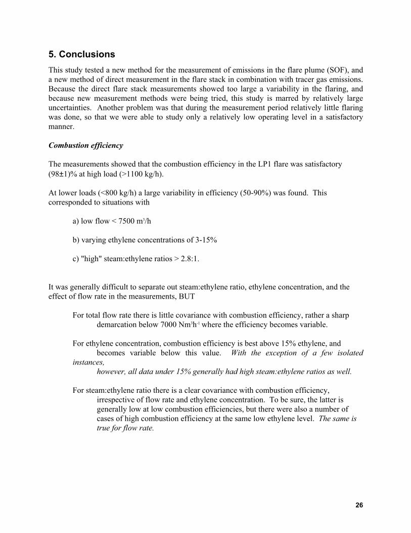
5. Conclusions This study tested a new method for the measurement of emissions in the flare plume (SOF), and a new method of direct measurement in the flare stack in combination with tracer gas emissions. Because the direct flare stack measurements showed too large a variability in the flaring, and because new measurement methods were being tried, this study is marred by relatively large uncertainties. Another problem was that during the measurement period relatively little flaring was done, so that we were able to study only a relatively low operating level in a satisfactory manner. Combustion efficiency The measurements showed that the combustion efficiency in the LP1 flare was satisfactory (98±1)% at high load (>1100 kg/h). At lower loads (<800 kg/h) a large variability in efficiency (50-90%) was found. This corresponded to situations with

a) low flow < 7500 m3/h

b) varying ethylene concentrations of 3-15% c) "high" steam:ethylene ratios > 2.8:1.

It was generally difficult to separate out steam:ethylene ratio, ethylene concentration, and the effect of flow rate in the measurements, BUT

For total flow rate there is little covariance with combustion efficiency, rather a sharp demarcation below 7000 Nm3h-1 where the efficiency becomes variable.

For ethylene concentration, combustion efficiency is best above 15% ethylene, and

becomes variable below this value. With the exception of a few isolated instances,

however, all data under 15% generally had high steam:ethylene ratios as well.

For steam:ethylene ratio there is a clear covariance with combustion efficiency, irrespective of flow rate and ethylene concentration. To be sure, the latter is generally low at low combustion efficiencies, but there were also a number of cases of high combustion efficiency at the same low ethylene level. The same is true for flow rate.

26

Emissions Emissions from the flares at both LP1 and LP2 were observed during most of the measurements. On August 8, 9, 22, 23 and 28 the instantaneous emissions from the LP1 flare varied between 5 and 200 kg⋅h-1. Even at good combustion efficiencies the emissions generally appear to vary between 20 and 50 kg⋅h-1 irrespective of quantity flared. The emissions from the LP2 flare seem to be of the same order of magnitude. The SOF measurements should not be used to estimate an annual mean emission from the flares, however, given that we measured only a few instantaneous emissions. In order to derive such an estimate it would be necessary to apply the calculated combustion efficiencies to various operating conditions. An emission of 20-50 kg⋅h-1 is, however, consistent with the long-term measurements done outside the plant. Emissions appear to increase at low load (lower flow rates), when the steam:ethylene ratio is generally high. The flares emit hydrocarbons when combustion is optimized for high loads (product discharges) and when the flares have a highly variable load over short time periods. The combustion efficiency at low loads is therefore very poor (50-90%), notably as a result of oversteaming in these situations. It was also our subjective impression from visits to the control room that the operators generally avoided soot formation at all costs and therefore tended to use a high steam setting. Automatic steam control is therefore needed in order to optimize the highly variable combustion.

27

28

6. References 1. Mellqvist, J., Galle, B., Arlander, D.W., Andreasson, K., Bergqvist, B., and Samuelsson, J. "Estimation of diffuse VOC emissions by long path FTIR measurements, tracer releases and time correlative analysis", in manuscript for Appl. Spectroscopy. 2. Mellqvist J, Galle, Bo, "Long-path-FTIR förِ Mätning av Diffusa Emissioner från Petrokemisk Industri" [Long-path FTIR for measuring diffuse emissions from the petrochemical industry], IVL report B1122, Göteborg, February 1994. 3. Mellqvist, J., Arlander, B. and Kloo, H., "Infraröd Fjärranalys för Mätning av Miljöstörande Gasformiga Ämnen i Verkstadsindustri" [Infrared remote sensing for measuring gaseous environmental contaminants in the manufacturing industry], IVL report B 1207, 1995. 4. Mellqvist, J., Arlander, D.W., Galle, B and Bergqvist, B., "Measurements of Industrial Fugitive Emissions by the FTIR-Tracer Method (FTM)", IVL report B 1214., 1995. 5. Mellqvist, J. and Samuelsson, J, "Automatic fugitive emission measurements using the FTC method", IVL report B 1335, 1999. 6. Pohl, Comb. Sci. and Tech., 50, 217-231, 1986. 7. Strosher, "Characterisation of Emissions from Diffusion flare systems", J. Air & Waste Management Assoc., 50:1723-1733, 2000. 8. Boden, Petroleum Review, 1996. 9. Blackwood, T., R., "An Evaluation of Flare Combustion Efficiency Using Open-Path Fourier Transform Infrared Technology", J. Air & Waste Management Assoc., 50:1714-1722, 2000. 10. Galle, B., Mellqvist, J., Arlander, D.W., Fliِsand, I., Chipperfield, M., and Lee, A.M., "Ground based FTIR measurements of stratospheric species from Harestua, Norway during SESAME and comparison with models", J. Atmos. Chem., 32, 1, 147-164, Journal of Atmospheric Chemistry, 1999 11. D. W. T. Griffith, Appl. Spectrosc., 50, 59, 1996