Public policies, regional inequalities and growth Philippe ... · Public policies, regional...

Journal of Public Economics 73 (1999) 85–105

Public policies, regional inequalities and growth

*Philippe MartinCERAS-ENPC, Graduate Institute of International Studies (Geneva), and CEPR,

`28 rue des Saints-Peres, 75343 Paris Cedex 07, France

Received 28 February 1998; received in revised form 31 August 1998; accepted 31 October 1998

Abstract

This paper constructs a two-region endogenous growth model where industrial locationand public infrastructures play a key role. The model analyzes the contribution of differenttypes of public policies on growth, economic geography and spatial income distribution. Itimplies that an improvement in infrastructures that reduces transaction costs inside thepoorest region decreases both the spatial concentration of industries, and the growth rate,and increases the income gap between the two regions. Conversely, an improvement ininfrastructure facilitating transactions between regions has the reverse effect. In this sense,the paper highlights a trade-off between growth and the spatial distribution of economicactivities. Contrary to transfers and traditional regional policies, it is shown that publicpolicies that reduce the cost of innovation can attain the objectives of higher growth andmore even spatial distribution of both income and economic activities. From that point ofview, these policies seem preferable to the regional policies now implemented in Europe. 1999 Elsevier Science S.A. All rights reserved.

Keywords: Growth; Geography; Infrastructure; Income inequalities; Public policies; Inno-vation

JEL classification: R58; 040; R12

1. Introduction

Is there a risk that integration in Europe increases regional income disparities?

*Fax: 133-1-4458-2880.E-mail address: [email protected] (P. Martin)

0047-2727/99/$ – see front matter 1999 Elsevier Science S.A. All rights reserved.PI I : S0047-2727( 98 )00110-8

86 P. Martin / Journal of Public Economics 73 (1999) 85 –105

Given the budget of the regional policies supposed to counteract this danger, theanswer of the governments is positive. The budget of regional policies hasincreased from ECU 3.7 billion in 1985 to ECU 18.3 billion in 1992 and will reachECU 33 billion in 1999. For the period 1994–1999, the Community’s budget forstructural policies represents a third of total spending, just after the CommonAgricultural Policy. These policies aim at financing public infrastructures, withspecial regard to transportation, in the poorest regions of Europe. This emphasis oninfrastructure is partly justified by the fact that disparities in infrastructure in theEU are greater than disparities in incomes.

This work originates from the belief that, given the huge sums spent on regionalpolicies and their political implications, it is important to develop an analytical

1framework to think about them. Regional policies are justified by the convictionthat the benefit accruing to poor regions might lead to a reduction in regionalinequalities profitable for Europe as a whole.

Why does the possibility of increased regional inequalities pose a problem topolicy makers? From an efficiency point of view, the answer is not obvious. Fujitaand Thisse (1996) insist on the economic gains produced by economic agglomera-tion such as localised technological or pecuniary positive externalities. However,the fact that regional inequalities might hurt immobile agents in declining regionsprovides a justification for all measures meant to diminish them, especially inEurope, where this problem is more acute than in the US.

This paper proposes an admittedly very partial and incomplete way to analyzesome of the effects of regional policies on industrial geography, regional incomedisparities and growth. With this aim, we use the model developed by Martin andOttaviano (1999) which marries an endogenous growth framework similar toRomer (1990) and Grossman and Helpman (1991) to a geography frameworksimilar to Helpman and Krugman (1985) and Krugman (1991). The role of publicinfrastructures in this endogenous geography and growth model will be introducedfollowing the static model in Martin and Rogers (1995).

The model studies two trading regions (North and South, with the North initiallyricher) where both capital flows and location choice are free. Transaction costsexist both between regions (inter-regional transaction costs) and inside regions(intra-regional transaction costs) and public infrastructures affect both kinds ofcosts. Given local technology spillovers, economic geography, described by theequilibrium location of industries, turns out to be a determinant of the commongrowth rate of innovation in the two regions. As transaction costs alter economicgeography, changes in infrastructures will have an effect not only on thegeography of the economic activities but also on the growth rate of the wholeeconomy, the differential in nominal income between regions and the income gap

1From an empirical perspective, see the papers in Haynes et al. (1996) on the role of infrastructuresin regional growth.

P. Martin / Journal of Public Economics 73 (1999) 85 –105 87

2between workers and capital owners. The model displays, from a theoretical point3of view, a policy trade-off between aggregate growth and regional equity. This

implies that regional policies that improve regional equity, improving, for instance,infrastructures in the poor region in order to attract firms, may not generate the

4geography most favourable to growth. Contrary to transfers and traditionalregional policies, we show that a public policy that reduces the cost of innovation,or other impediments to growth, attains both the objectives of higher growth andregional equity.

The next section introduces the basic features of the model, especially publicinfrastructures. Section 3 derives the equilibrium location of firms. Section 4shows how the growth rate of the economy depends on geography and Section 5determines income inequality. Section 6 analyzes the impact of different publicpolicies.

2. A two-region model with infrastructures

We consider two regions, North and South, each endowed with a fixed amountof labour (L) immobile between regions so as to abstract from that particularagglomeration channel. The regions are identical except for their initial incomelevel.

Given the symmetry of the model, we concentrate on the specification of theNorth (variables referring to South are labelled by an asterisk). Preferences areinstantaneously nested-C.E.S. and intertemporally C.E.S., with unit elasticity ofintertemporal substitution:

`

a 12a 2r tU 5E log[D(t) Y(t) ]e dt (1)0

Y is the consumption of the homogeneous good (an agricultural good forexample), r the rate of time preference and a[(0, 1) the share of expenditures

2Benabou (1993) and Benabou (1994) analyze a related question, the impact of local human capitalexternalities on growth and income inequality. His focus however is on education and incomeinequality across agents in urban areas.

3Quah (1996) and Martin (1998) provide some empirical evidence for such trade-off for Europeanregions. Quah finds that European countries which did not experience rising regional inequalities hadlower growth.

4Martin and Ottaviano (1999) analyze this trade-off from a welfare point of view to show that theoptimal geography may entail more or less spatial concentration than the market equilibrium dependingon the level of transaction costs. Matsuyama and Takahashi (1998) present a model where economicgeography can be characterized by excessive or insufficient agglomeration due to the absence of certainmarkets and the lack of coordination of agents.


devoted to D. The latter is a composite good that, following Dixit and Stiglitz(1977), consists of a number of different varieties:

N(t ) 1 / (121 /s )

121 /sD(t) 5 OD (t) s . 1 (2)F Gii51

where N is the total number of varieties available in the economy. s is theelasticity of substitution between varieties, as well as the own-price elasticity ofthe demand for each of them. Growth will come from an increase in the variety ofgoods measured by N.

The value, in terms of the numeraire Y, of per capita expenditure E is:

n N

*E 5Ot p D 1 O t p D 1 Y (3)D i i I j ji51 i5n11

where n is the number of goods of the manufacturing sector produced in region 1and N5n1n*. As in Samuelson (1954) and in the economic geography literature,transaction costs have been introduced. These, in the form of iceberg costs, affectboth intra-regional (t ) and inter-regional transactions (t ). Both t and t areD I D I

larger than 1 so that only a fraction of the good or service purchased is actuallyconsumed. The quality of infrastructures in the North and the South can differ so

*we consider t ±t . However, we will assume that the infrastructure thatD D

*facilitates transactions between them is shared by the two regions so that t 5tI I

*and that t .t $t . This assumption implies that it is more costly to trade withI D D

an agent from the other region than with an agent in the same region and that thecost of intra-regional transactions in the North is at least as low as in the South. Asin Martin and Rogers (1995), we interpret these costs as directly related to thequality of infrastructures. We will regard a reduction of t (t ) as an improvementD I

of intra-regional (inter-regional) infrastructure. Transaction costs affected bypublic infrastructures can be conceived as transport and telecommunicationinfrastructures. For example, the construction of a highway between Milan andNaples will be as an improvement in inter-regional infrastructure while a roadbetween Milan and Florence as an improvement of intra-regional infrastructure of

5Northern Italy. As is common in the new geography models, there is notransaction cost for the numeraire good introduced to tie down the wage rate.

As to the supply side, the homogenous good is produced using only labour withconstant returns to scale in a perfectly competitive sector. Without loss ofgenerality, the input requirement is set to 1 for convenience. It is assumed that thedemand for this good in the whole economy is large enough that, since it is not

5For a more detailed explanation of this way of modelling of infrastructures see Martin and Rogers(1995).


satisfied by production in only one region, in equilibrium the production is carriedout in both. Free trade guarantees that the nominal wage rates are equalised acrossregions, while the assumption of unit input requirement and the choice of Y as thenumeraire pin down the wage rate to 1 everywhere.

The differentiated good or service is produced in a monopolistically competitivesector with increasing returns to scale in the production of each variety. This,together with the assumption of costless differentiation, ensures that each firm willproduce only its own variety. More precisely, starting the production process foreach new variety requires the use of one unit of capital (the fixed cost at the source

6of economies of scale ) and b units of labour. As labour is the only productionfactor in this increasing returns sector, we can think of its output as either goods orspecialised services. Under these assumptions, optimal pricing for any varietygives producer prices, such that: p5p*5bs/(s21). The operating profits of aproducer are

bx]]p 5 px 2 bx 5 (4)s 2 1

where x is the optimal output / size of a typical firm in equilibrium.Investment is needed to produce a new variety. This can be thought about as

either the innovation required to start production of a new good or the physicalinvestment to open a plant. In the first case, capital is immaterial, i.e. a patent, inthe second, a piece of machinery. Here, we will interpret capital as a composite ofthese two. In both cases, the value of the firm that produces the new variety is thevalue of its capital unit. Once investment is performed, the entrepreneur hasmonopoly rights on the variety produced and the choice to freely relocate theproduction facilities across regions. This implies that there are no relocation costson capital, be it a patent or a machine. If the entrepreneur decides to locate theproduction facility in the region where she does not live, she will repatriate the

*profits. Initially, the North owns H units of capital and the South H with0 0

*H .H . The requirement that one unit of capital is used to start the production0 0

process for each variety implies that the total number of varieties and firms in theworld is fixed by the stock of capital at each point in time: N5n1n*5H 1H*.

Finally, we assume that there exists a safe asset, bearing an interest rate r inunits of the numeraire, whose market is characterised by free financial movementsbetween the two regions. The intertemporal optimisation by consumers then

~ ~implies that the growth rate of expenditure is E5E*5r2r, the differencebetween the interest rate and the rate of time preference. It turns out that in steadystate E and E* must be constant so that r5r.

6This way of introducing economies of scale has been used in Flam and Helpman (1987) in a tradecontext and Martin and Rogers (1995) in a geography context.


3. The equilibrium location of firms

Given the absence of restrictions on inter-regional capital flows, the equilibriumlocation is such that operating profits of firms are equal in both regions. Noincentive to relocate production can exist in equilibrium. Hence, it must be p5p*which implies x5x*. The next equilibrium condition is that demands (inclusive oftransaction costs) equal supplies. The first order conditions for consumers give theusual demands for the different goods, so we get:

Ed E*daL(s 2 1) D I]]] ]]]]]] ]]]]]]x 5 1 (5a)S Dbs *N[gd 1 (1 2 g )d ] N[gd 1 (1 2 g )d ]D I I D

*Ed E*daL(s 2 1) I D]]] ]]]]]] ]]]]]]x* 5 1 (5b)S Dbs *N[gd 1 (1 2 g )d ] N[gd 1 (1 2 g )d ]D I I D

where g5n /N, the share of varieties produced in region 1, is less or equal to 1. g

will be a crucial parameter of the model as it measures the extent of agglomeration12s *of the manufacturing sector in region 1. To simplify, we define d 5t . d , dD D I D

are defined similarly. A higher d implies a better infrastructure facilitatingD

intra-regional transactions in the North. This system can be solved for theequilibrium location:

*u d (1 2u )dE D E I]]] ]]]g 5 2 (6)*d 2 d d 2 dD I D I

where u 5E /(E1E*) is the Northern share of total expenditure or income. ThisE

equation gives the equilibrium location of firms as a function of expenditures andinfrastructures in the North and in the South. We can see that, as in the new tradetheory and in the new geography, a ‘home market’ effect exists since a higherlevel of local expenditures attracts firms, due to increasing returns in thedifferentiated goods sector. We come back to the other determinants of location,and, in particular, to public infrastructures in Section 6.

The optimal size of firms in both the South and the North is then:

s 2 1 E 1 E*]]]]x 5 aL (7)

bs N

4. Equilibrium growth

The next step is to find the growth rate in this economy, that is how capital isendogenously accumulated. The innovation sector works as in Grossman andHelpman (1991): to build one more unit of the composite capital required to startproduction in the differentiated goods sector, an entrepreneur must employ h /nunits of labour in the North and h /n* in the South. This implies that, as in Martinand Ottaviano (1999), there exists a local spillover that makes the cost of


innovation in a region a decreasing function of the number of firms already located7in that region, that is, a function of the diversity of the industrial structure.

What is the empirical evidence underlying this type of spillover? Using theterminology of Glaeser et al. (1992), localised spillovers may be either of theMarshall–Arrow–Romer (MAR) type or of the Jacobs (1969) type. The former aregenerated by interactions among local firms in the same industry. In the latter localindustrial diversity plays a positive role in fostering innovation and the build-up ofknowledge and ideas. Here, the spillovers are of the second type, with the diversityof the industrial sector being a key factor. Jaffe et al. (1993), and Henderson et al.(1995) find evidence for Jacobs’ spillovers. In particular, the latter show that newhigh-tech industries are more likely to take root in cities with a history ofindustrial diversity. Ciccone and Hall (1996) also show that there is a positiverelation between density and productivity at the state level in the US, consistentlywith the effect of the spillovers we assume.

The fact that it is less costly to engage in investment in the region with a highershare of firms immediately implies that all the investment activity will take place

8there. As capital can freely relocate, its price and, therefore, its cost has to be thesame in both regions, for them to engage in investment. In equilibrium, more firmsoperate in the North than in the South, so that the investment sector will only beactive in the North, where the growth rate of the country will be determined.

A steady state of the model is defined as an equilibrium where g5n /N, theproportion of firms in region 1, is constant so that n, n* and N grow at the same

~constant rate g5N /N. To find the equilibrium growth rate, we must analyze theincentive to develop new varieties and firms. Calling v the value of a firm, whichis also the value of its capital unit, the condition of no arbitrage opportunitybetween shares and the safe asset implies:

~v p] ]r 5 1 (8)v v

On an investment of value v, the return is equal to the operating profits plus thechange in the value of capital. This condition could also be derived by stating thatthe equilibrium value of a firm is the discounted sum of its future profits. Givenfree entry and zero profits in the investment sector, the value of a firm is equal tothe marginal cost of the unit of capital required to start production in the firm:v5h /n is therefore another equilibrium condition so that v decreases at the rate ofgrowth of n:

7Another way to get to the same type of result without assuming local technological spillovers is tointroduce a pecuniary externality as in Martin and Ottaviano (1996). In this model, the innovationsector requires manufacturing goods which also incur transaction costs so that if industrial con-centration increases, the cost of inputs for the innovation sector decreases.

8Audretsch and Feldman (1996) find that R&D activities are more concentrated spatially thanproduction activities, consistent with our model.


~ ~ ~g 5 N /N 5 n /n 5 2 v /v

Another equilibrium relation is the market clearing condition on the labourmarket. It implies that labour (2L) will be employed either in the R&D sector

~(hN /n), the constant returns sector (LY1LY*) or the increasing returns sector(Nbx):

~N s 2 a] ]]2L 5h 1 LY 1 LY* 1 Nbx 5hg /g 1 L(E 1 E*) (9)n s

If a steady state exists with g and g constant, then the equation above impliesthat expenditures must also be constant. In turn, intertemporal optimisation impliesthat r5r. Given this and the marginal cost pricing of capital (v5h /n), thearbitrage condition (8) can be rewritten as: g1r5(pn) /h. Using the equilibriumprofits p in (4), the equilibrium size of firms in (7) and Eq. (8) and Eq. (9), it iseasy to find the growth rate:

2L a s 2 a]] ]]g 5 g 2 r (10)h s s

Some of the usual determinants of growth in endogenous growth models arepresent here. A higher r decreases the growth rate through an increase in presentconsumption at the expense of saving and investment in the innovation sector. Alarger population L increases growth because of the usual scale effect. A higherelasticity of substitution between varieties (s) decreases the monopoly power ofeach firm and, therefore, the incentive to create new firms. A higher cost ofinnovation, measured by h, also decreases the growth rate. Because of the localspillovers, the concentration of economic activities, g, has a positive effect ongrowth as it decreases the cost of investment in the North, the region specialised inthis activity (see Martin and Ottaviano, 1999).

Note also that the growth rate given in (10) is the common growth rate of H,H*, n, n* and N. Free capital mobility ensures that the North and the South canaccumulate capital at the same rate. The North innovates and produces newcapital, an activity that generates no profits. The South can and will buy some ofthese units of capital at the same rate as the North.

5. Equilibrium income inequality

The two preceding sections have determined the equilibrium location of firms,g, as a function of the income inequality u , and the equilibrium growth rate, g, asE

a function of g. To complete the solution of the model we have to determine howincome inequality depends on the growth rate of the economy.

Per capita income levels in both regions are the sum of labour income, 1 in both


regions, and capital income given by the product of total wealth and the propensityto consume (r, in our log utility case). In other words, instantaneous capitalincome is wealth multiplied by the equilibrium return, r5r. Per capita wealth inthe North is then simply the constant Hv /L, as the capital stock H is rising at thesame rate as v is decreasing. Aggregate income in the world is then: (E1E*)L5

2L1rNv. The value of capital, given by the arbitrage condition (8) v5p /(r1g),is the discounted sum of future profits. It is lower, the higher the growth rate sincefuture profits decrease if more firms are created and enter the market. Using theseidentities and the equilibrium value of profits given by Eq. (4) and Eq. (7), we canfind how income levels depend on the growth rate:

2arh 2ar(1 2 h)]]]]] ]]]]]E 5 1 1 ; E* 5 1 1 (11)(s 2 a)r 1 sg (s 2 a)r 1 sg

where h5H /N is the share of capital owned by the North. Note that this share isconstant over time as H, H*, N and N* grow at the same rate in both regions.u 5E /(E1E*), the consumers’ share of expenditures and income in the North, isE

therefore:

1 s( g 1 r) 1 ar(2h 2 1)]]]]]]]]u 5 (12)E 2 s( g 1 r)

Note that as long as h.1/2, that is, as long as the North is initially betterendowed in capital than the South, then u .1/2, that is, income per capita isE

higher in the North than in the South. This is the case as we assumed the North*initially richer than the South (H .H ) and the growth rate of capital common to0 0

both regions. Note also that income inequality is decreasing in the growth rate.The reason is that the value of capital is lower with higher growth because of morefuture competition due to faster entry of new firms. As the North is relatively richin capital (h.1/2), the level of capital income declines more in the North than inthe South, leading to decreasing income inequality.

We can also look at the relation between geography, g, and income inequality uE

by using Eq. (10) and Eq. (12):

gL 1 rhh]]]u 5 (13)E 2gL 1 rh

The expenditure and income share in the North decreases with g, the share offirms locating in the North. This follows from the fact that industrial concentrationin the North, reducing the cost of innovation, increases the growth rate and curtailsthe monopoly power of existing firms. This effect, that can be considered as acompetition effect, implies that the equilibrium geography is stable: in general, notall firms will decide to produce in the North. There are several reasons for that.First, the competition effect drives firms owned by Northerners to relocateproduction in the South where competition is less fierce. Second, there is free


capital mobility. This allows Southerners to invest in capital accumulated in theNorth (in the form of patents or shares). Hence, the lack of an innovation sectordoes not prevent the South from accumulating capital: the initial inequality inwealth does not lead to self-sustaining divergence. No ‘circular causation’mechanism which would lead to a core-periphery pattern, as in the ‘newgeography’ models of the type of Krugman (1991), will occur. Here, theintroduction of endogenous capital and free capital movements gives rise to the

9possibility of a stable interior solution equilibrium.Using Eq. (6) and Eq. (13), the equilibrium g is the solution to a quadratic

equation given in Appendix A. The equilibrium growth rate follows from Eq. (10).

6. Geography, growth and public policies

We are interested in the impact of the different types of public policies on theindustrial geography, g, on the geography of incomes and expenditures, u , and onE

the growth rate of innovation, g, that applies to the whole country. The location offirms matters for immobile agents in our set-up because a region that has morefirms also benefits from a lower price index. This is due to the fact that for locallyproduced goods, transaction costs (intra-regional) are less than for goods imported

*from the other region because: d .d .d . The price index that corresponds toD D I1 / (12s) 1 / (12s)our nested CES utility function is: P5(bs/(s21))N [gd 1(12g)d ]D I

1 / (12s) 1 / (12s)*in the North and P*5(bs/(s21))N [gd 1(12g)d ] in the South.D I

Hence, an increase in spatial concentration in the North, g, benefits consumers inthe North and hurts consumers in the South. As more goods are produced in theNorth and less in the South, consumers in the North pay less while consumers inthe South pay more.

The disparity in real income across the regions depends on the disparity innominal incomes, u , given by Eq. (12), and on the disparity in the price indicesE

defined above which itself depends on g. If g and u , industrial agglomeration andE

nominal income disparity, go in the same direction, then the impact on real incomedisparity is unambiguous. For example, an increase in g and u implies that realE

income disparities increase between the North and the South as nominal incomedisparities increase at the same time as the price index decreases in the North andincreases in the South. On the contrary, if nominal income disparity increases butindustrial agglomeration decreases, the effect on real income inequality isambiguous. In general, the impact of industrial agglomeration on the price indexwill be less important the better the public infrastructures. In particular, ifinter-regional transaction costs are not very high, then the location of production

9See Baldwin (1998) and Baldwin et al. (1998) for models of growth and geography withcatastrophic agglomeration due to imperfect capital mobility.


will have little effect on the price indices and, therefore, on the real incomedisparities. In this case, the real income disparities will follow the nominal income

10disparities.We can analyze the nature of the equilibrium and the effects of various public

policies graphically. Eq. (6) provides a positive relation between g and u , theE

‘home market’ effect. In Graph 1, this relation is given by the curve g(u ) in theE

NE quadrant. Eq. (10) provides a positive relation between g and g. This is thespillovers effect: when industrial agglomeration increases in the region where theinnovation sector is located, the cost of innovation decreases and the growth rateincreases. This relation is given by the line g(g) in the NW quadrant. Finally, Eq.(12) provides a negative relation between u and g. This is the ‘competition’E

effect: the monopoly profits of existing firms decrease as more firms are created.As the North is more dependent on this capital income, the Northern share ofincome and, therefore, of expenditures decreases. This relation is described by thecurve u ( g) in the SE quadrant.E

Graph 1. Equilibrium growth, agglomeration and income inequality.

10For a more detailed analysis of welfare effects of location see Martin and Ottaviano (1999).


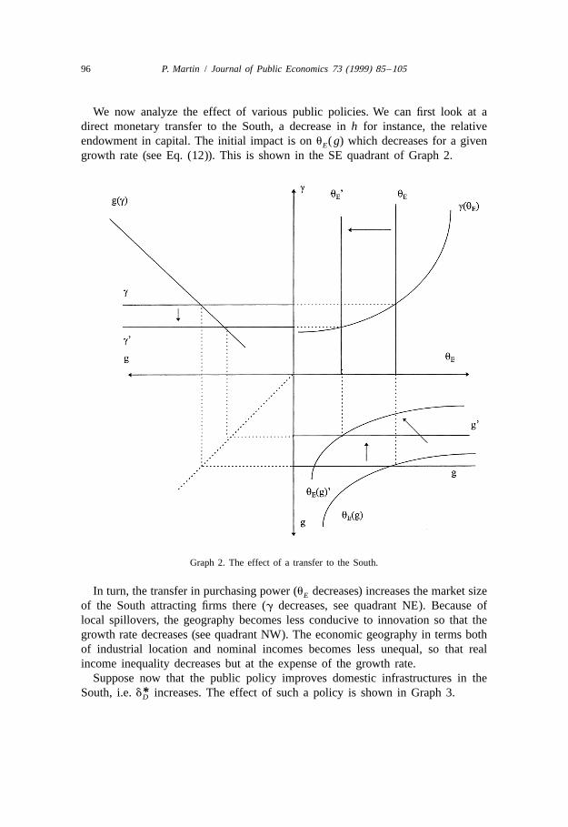
We now analyze the effect of various public policies. We can first look at adirect monetary transfer to the South, a decrease in h for instance, the relativeendowment in capital. The initial impact is on u ( g) which decreases for a givenE

growth rate (see Eq. (12)). This is shown in the SE quadrant of Graph 2.

Graph 2. The effect of a transfer to the South.

In turn, the transfer in purchasing power (u decreases) increases the market sizeE

of the South attracting firms there (g decreases, see quadrant NE). Because oflocal spillovers, the geography becomes less conducive to innovation so that thegrowth rate decreases (see quadrant NW). The economic geography in terms bothof industrial location and nominal incomes becomes less unequal, so that realincome inequality decreases but at the expense of the growth rate.

Suppose now that the public policy improves domestic infrastructures in the*South, i.e. d increases. The effect of such a policy is shown in Graph 3.D


Graph 3. The effect of a decrease of intra-regional transaction costs in the South.

In this case, as easily checked from Eq. (6), g decreases for any given level ofu (see quadrant NE in Graph 3; g(u ) shifts to the right). The intuition is that, asE E

public infrastructure improves, transaction costs on goods produced and consumedin the South decrease, increasing the effective demand. Given increasing returns toscale, firms in the differentiated goods sector relocate to the South and g

decreases. Relocation from the North, where the innovation sector is located, to theSouth brings about an increase in the cost of innovation reducing the growth rateof innovation. In this sense, the improvement in infrastructure of the Southgenerates a less growth conducive geography and, through a reduction in thegrowth rate of innovation, it lessens competition, increasing monopoly profits tothe benefit of capital owners in both regions. As capital owners are more numerousin the North, the inter-regional inequality in expenditures, measured by u , risesE

(see quadrant SE). The net effect on real income inequality is however ambiguous.Nominal income inequality has increased but the price index has decreased in the


South compared to the North. This is due to the fact that more firms produce in theSouth and that the cost of transporting locally produced goods to consumers in theSouth has decreased.

Note also that economic geography has not only an impact on inter-regionalincome inequality but also on a particular form of intra-regional inequalitybetween workers and capital owners. When monopolistic profits increase due to aless concentrated geography (higher g) and a lower growth rate, this increases therelative income gap between capital owners and wage earners. This is true in bothregions.

We do not take into account the cost of such a policy. If this improvement ininfrastructure is paid for by a monetary transfer by the North as is the case forregional policies, then the effect will be the combination of those studied in Graph2 and Graph 3. Taking into account the financing would therefore reinforce theimpact on the growth rate and on industrial agglomeration but would make theeffect on nominal income inequality ambiguous.

Graph 4. The effect of a decrease of inter-regional transaction costs.


Graph 4 analyses the effect of improving infrastructure that helps inter-regionaltrade (an increase in d ). In this case, as long as the North has a larger market sizeI

than the South, this improvement in inter-regional infrastructure will increase theattractiveness of the North, that is: ≠g/≠d .0 in Eq. (6) (see proof in Appendix B)I

for a given income inequality. Hence, g(u ) shifts as shown in quadrant NE andE

the effect of such policy is qualitatively the exact opposite to the effect of adecrease of intra-regional transaction costs in the South analyzed in Graph 3.

As trade towards the South is made easier, it is less necessary to locateproduction in the South and firms can now take advantage of the scale economiesin the North. The North can have a larger market either because it is richer(h.1/2) and/or because it has better domestic infrastructure than the South

*(d .d ). In the latter case, its effective demand is larger because less of the goodD D

produced in the Northern region is lost in transit for the consumers in the North.Hence, in this case, an improvement in inter-regional infrastructure has theopposite effect of an improvement in intra-regional infrastructure in the South: asg increases, the growth rate of innovation, g, increases, and u decreases asE

monopolistic profits of each capital owner decrease.The impact on real income disparities is ambiguous: nominal income disparities

decrease but the impact on the price index in the two regions is more complex. Inthe South as d increases, the cost of importing goods from the North decreases.I

However, as some firms relocate to the North (g increases), more of the goodshave to be imported bearing a higher transaction cost (the inter-regional one) thanthe one faced if the good was produced locally. It can be shown (see Appendix C)that the first effect is larger than the second so that, following a decrease in theinter-regional transaction cost, the price index in the South decreases. In the North,both effects go in the same direction: the cost of importing goods from the Southdecreases and more firms decide to produce in the North. It can be shown that theprice index decreases more in the South than in the North. The net effect on realincome inequality is therefore ambiguous. As shown in Martin and Ottaviano(1999), if transaction costs between the two regions are already sufficiently low,the impact on price indices will not be very important. So, an improvement ininfrastructures that help decrease the inter-regional transaction costs further willlower real income inequality between the regions.

A decrease in the intra-regional transaction costs in the North would have thesame qualitative effect as those described here for the improvement of inter-regional infrastructures.

To take into account the effect of financing these infrastructures by the North,we need to combine the effects described in Graph 2 and Graph 4. The effect onnominal income inequality would be reinforced but the impact on the growth rateand on agglomeration would become ambiguous. If the unwelcome effect of sucha policy (the increase in industrial agglomeration) were then reversed, it wouldimply that its induced positive impact on growth would also be reversed.

In the case of the public policies described above, all regional in nature, a


trade-off exists because they all have an undesirable side effect. They either lead tolower growth (the direct transfer to the South, the improvement of intra-regionalinfrastructures in the South) or to higher nominal income inequality (theimprovement in intra-regional infrastructures) or to more industrial agglomeration(the improvement in inter-regional infrastructures). Taking into account the cost offinancing these policies does not change this conclusion.

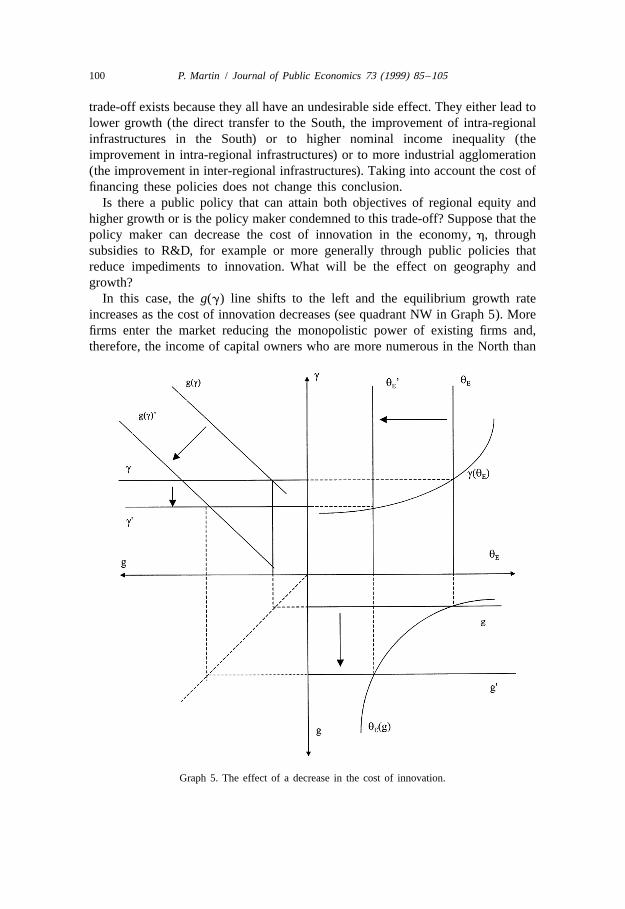
Is there a public policy that can attain both objectives of regional equity andhigher growth or is the policy maker condemned to this trade-off? Suppose that thepolicy maker can decrease the cost of innovation in the economy, h, throughsubsidies to R&D, for example or more generally through public policies thatreduce impediments to innovation. What will be the effect on geography andgrowth?

In this case, the g(g) line shifts to the left and the equilibrium growth rateincreases as the cost of innovation decreases (see quadrant NW in Graph 5). Morefirms enter the market reducing the monopolistic power of existing firms and,therefore, the income of capital owners who are more numerous in the North than

Graph 5. The effect of a decrease in the cost of innovation.


in the South. This reduces the income differential between North and South,between workers and capital owners inside each region, and leads to firms’relocation to the South.

It can be shown that in Eq. (10), the exogenous decrease in the cost ofinnovation more than compensates the endogenous decrease in spatial con-centration (the decrease in g) so that the net effect is an increase in the growth rate(see proof in Appendix D). Hence, a public policy that reduces the cost ofinnovation can attain both the objectives of higher growth and more equity. Bothindustrial concentration in the North and the income differential between Northand South decrease so that the real income differential unambiguously decreases.If subsidies to R&D, increased competition on goods markets and labour markets,improved education infrastructure, etc., can decrease the cost of innovation forfirms, then, this kind of policy may yield more desirable outcomes than traditionaltransfers or regional policies. Note that such a policy, leading to the relocation ofeconomic activities to the South, helps the creation of new economic activities andfirms without any of the local bias that regional policies usually have.

Taking into account the financing of such a policy by the North (combining theeffects described in Graph 2 and Graph 5) does not reverse these conclusions. Theimpact on nominal income inequality and industrial agglomeration would bereinforced. The net impact on growth may turn negative if the financial burden ofthe policy is so high that the effect on incomes and geography dominates the directeffect on the cost of innovation. This just says that the cost of such a policy shouldnot be too high to have the desired effect on growth.

7. Conclusion

This paper has presented a simple model of growth, geography and publicpolicies. Even in such a simple framework, some interesting results can emerge.Given that economic geography affects growth, public policies that alter industriallocation also affect growth. We have shown that the problem with public policiesattempting to affect economic geography through infrastructure or throughtransfers, presumably to generate a more equal spatial distribution of economicactivities, is that, if they obtain this result, the consequence may be lower growthfor both regions. This is due to the fact that the presence of local spillovers impliesthat spatial industrial concentration is conducive to lower costs of innovation.Hence, a trade-off exists between spatial equity in industrial location andaggregate growth. From this point of view, a more specialised and concentratedeconomic geography is preferable. On the other hand, such an economicgeography is detrimental to immobile workers in the poor region because, furtheraway from the main production site, they have to pay higher transaction costs.Regional policies either in the form of an improvement in public infrastructures


that favour intra-regional trade or in the form of direct transfers to a poor regionhave to face this trade-off.

We have shown that the geography of industry location and income may berelated in an interesting way. An increase in spatial concentration of firms in theNorth leads to a decrease in nominal income disparities between North and Southbecause the competition effect that follows leads to a decrease of the monopolisticprofits on which the North is more dependent than the South. A related point isthat policies that affect industrial geography, have an impact on income inequalityinside each region because they affect monopolistic profits of capital owners.

Policies that lead to a decrease in the cost of innovation, through subsidies forexample, can lead to higher growth, lower monopolistic profits for capital ownersand more even spatial distribution of incomes and economic activities. From thispoint of view, these policies seem preferable to the regional policies now in favourin Europe.

To our knowledge, this paper is the first to analyze in an integrated frameworkthe role of public policies, especially public infrastructure policies, on growth,income and economic geography. Admittedly, our model is very incomplete andspecial in some of its assumptions so that our results may be too unfair to regionalpolicies. Its main point, however, is to clarify some economic mechanisms thatexplain why regional policies can have complex and undesirable consequences andwhy they can have not only a local impact but also a national impact.

Acknowledgements

I thank Harry Flam, Richard Baldwin, the editor Roger Gordon and twoanonymous referees for helpful suggestions that led to substantial revisions. TheSwiss National Science Foundation Grant 12-50783.97 provided support for thisresearch.

Appendix A

The quadratic equation that determines the equilibrium g is:

2 * * *2g L(d 2 d )(d 2 d ) 2 g [Ld (d 2 d ) 2 Ld (d 2 d )D I D I D D I I D I

* *2 rh(d 2 d )(d 2 d )] 2 rh[hd (d 2 d )D I D I D D I

*2 (1 2 h)d (d 2 d )] 5 0 (A1)I D I

The valid solution (the other root is more than 1) is:


]Œ* * *Ld (d 2 d ) 2 Ld (d 2 d ) 2 rh(d 2 d )(d 2 d ) 1 DD D I I D I D I D I]]]]]]]]]]]]]]]]g 5 *4L(d 2 d )(d 2 d )D I D I

2* * *D 5 [Ld (d 2 d ) 2 Ld (d 2 d ) 2 rh(d 2 d )(d 2 d )]D D I I D I D I D I(A2)

* * *1 8Lrh(d 2 d )(d 2 d )[hd (d 2 d ) 2 (1 2 h)d (d 2 d )]D I D I D D I I D I

This root is less than 1, i.e. there is less than full agglomeration of economic*activities in the North, if h, d and the difference between d and d are not tooI D D

large. The equilibrium value of u follows from Eq. (13) and the equilibrium valueE

of g follows from Eq. (10).

Appendix B

The partial derivative of g with respect to d in Eq. (6) is:I

*u d (1 2u )d (1 2u )≠g E D E I E] ]]] ]]] ]]]5 2 2 (A3)2 2≠d (d 2 d )*(d 2 d ) (d 2 d )I D ID I D I

To look separately at the role of differences in income and in infrastructurelevels, first assume that domestic infrastructures are of the same quality in both

*regions i.e. d 5d then:D D

(2u 2 1)d≠g E D] ]]]]5 2≠d (d 2 d )I D I

This is positive as long as u .1/2 that is as long as the North has a largerE

expenditure level than the South. This is the case as we assume that the North isinitially richer in capital than the South: h.1/2 (see Eq. (11)).

Suppose now that there is no difference in expenditure levels between North andSouth so that h5u 51/2, then:E

2* *(d d 2 d )(d 2 d )≠g D D I D D] ]]]]]]]5 (A4)2 2≠d *2(d 2 d ) (d 2 d )I D I D I

This expression is positive as the first term in the numerator is positive becauseof our assumption that the inter-regional transaction costs are larger than theintra-regional costs, and the second term is positive as long as domesticinfrastructure in the North is better than domestic infrastructure in the South.


Appendix C

We analyze the impact of an improvement in inter-regional infrastructures on*the price indices of the regions in the case where d 5d :D D

1 1≠P* bs 1 ≠g] ]2112s 12s]] ]] ]] ]S D5 2 N [(1 2 g )d 1 gd ] g 1 (d 2 d )F GD I I D≠d s 2 1 s 2 1 ≠dI I

1 1bs 1] ]2112s 12s]] ]]S D5 2 N [(1 2 g )d 1 gd ] (1 2u ) , 0D I Es 2 1 s 2 1

1 1≠P* bs 1 ≠g] ]2112s 12s]] ]] ]] ]S D5 2 N [gd 1 (1 2 g )d ] 1 2 g 2 (d 2 d )F GD I I D≠d s 2 1 s 2 1 ≠dI I

1 1bs 1] ]2112s 12s]] ]]S D5 2 N [gd 1 (1 2 g )d ] (1 2u ) , 0D I Es 2 1 s 2 1

(A6)

Hence both price indices decrease. Using the results above, and the fact thatu .1/2 and gd 1(12g)d .(12g)d 1gd it can be proved that a ≠(P/P*) /E D I D I

≠d ,0, so that the relative price index changes in favour of the North.I

Appendix D

We want to prove that dg /dh is negative. From Eq. (10), we see that this isequivalent to proving that e5(dg/g) /(dh /h) is less than 1. We will prove this for

*the case when d 5d . For this, we differentiate Eq. (6) and Eq. (13) in the textD D

and eliminate du . After simplification, one gets the following elasticity:E

Lrh(2h 2 1)(d 1 d )≠g h D I]] ]]]]]]]]]]]]]5 2≠h g Lrh(2h 2 1)(d 1 d ) 1 (d 2 d )(2Lg 1 rh)D I D I

which is less than 1 as h.1/2.

References

Audretsch, D.B., Feldman, M., 1996. R&D spillovers and the geography of innovation and production.American Economic Review 86 (3), 630–640.

Baldwin, R.E., 1998. Agglomeration and endogenous capital. European Economic Review, in press.Baldwin, R.E., Martin, P., Ottaviano, G., 1998. Global income divergence, trade and industrialisation:

the geography of growth take-offs. NBER working paper no. 6458.Benabou, R., 1993. Workings of a city: location, education and production. Quarterly Journal of

Economics 108, 619–652.


Benabou, R., 1994. Human capital, inequality and growth: a local perspective. European EconomicReview 817–826.

Ciccone, A., Hall, R., 1996. Productivity and the density of economic activity. American EconomicReview 87 (1), 54–70.

Dixit, A., Stiglitz, J., 1977. Monopolistic competition and optimum product diversity. AmericanEconomic Review 67 (2), 297–308.

Flam, H., Helpman, E., 1987. Industrial policy under monopolistic competition. Journal of InternationalEconomics 22, 79–102.

Fujita, M., Thisse, J.F., 1996. Economics of agglomeration. Journal of Japanese and InternationalEconomics 10, 1–40.

Glaeser, E.L., Kallal, H., Scheinkman, J., Schleifer, A., 1992. Growth in cities. Journal of PoliticalEconomy 100, 1126–1152.

Grossman, G., Helpman, E., 1991. Innovation and Growth in the World Economy. MIT Press,Cambridge, MA.

Haynes, K., Button, K., Nijkam, P., Qiangshang, L., 1996. Regional Dynamics, vol. 2. Edward Elgar.Helpman, E., Krugman, P., 1985. Market Structure and Foreign Trade. MIT Press, Cambridge, MA.Henderson, V., Kuncoro, A., Turner, M., 1995. Industrial development in cities. Journal of Political

Economy 103 (5), 1067–1090.Jacobs, J., 1969. Economy of Cities. Vintage, New York.Jaffe, A., Trajtenberg, Henderson, R., 1993. Geographic localization of knowledge spillovers as

evidenced by patent citations. Quarterly Journal of Economics 108, 577–598.Krugman, P., 1991. Increasing returns and economic geography. Journal of Political Economy 99,

483–499.Martin, P., 1998. Can regional policies affect growth and geography in europe?. World Economy 21,

757–774.Martin, P., Ottaviano, G.I.P., 1996. Growth and agglomeration. CEPR discussion paper 1529.Martin, P., Ottaviano, G.I.P., 1999. Growing locations: industry location in a model of endogenous

growth. European Economic Review 43, 281–302.Martin, P., Rogers, C.A., 1995. Industrial location and public infrastructure. Journal of International

Economics 39, 335–351.Matsuyama, K., Takahashi, T., 1998. Self-defeating regional concentration. Review of Economic

Studies 65 (2), 211–234.Quah, D., 1996. Regional Cohesion from Local Isolated Actions: 1. Historical Outcomes. LSE, mimeo.Romer, P., 1990. Endogenous technical change. Journal of Political Economy 98 (5), S71–S102.Samuelson, P., 1954. The transfer problem and transport costs, II: analysis of effects of trade

impediments. Economic Journal 64, 264–289.

Public policies, regional inequalities and growth Philippe ... · Public policies, regional...

Documents

Transcript of Public policies, regional inequalities and growth Philippe ... · Public policies, regional...