Public Facility Planning Models

with Single and Multiple Services:

Models, Solution Methods and Applications

Doctoral thesis

Thesis submitted to the Faculty of Sciences and Technology of

the University of Coimbra in partial fulfillment of the requirements for

the degree of Doctor of Philosophy in the field of Civil Engineering,

with specialization in Spatial Planning and Transportation.

Author

João Carlos Vicente Teixeira

Supervisors

António Pais Antunes (University of Coimbra, Portugal)

Laurence A. Wolsey (Catholic University of Louvain, Belgium)

Coimbra, June 2012

iii

Financial support

This work had the financial support of Fundação para a Ciência e a Tecnologia (FCT,

Portugal) through doctoral degree grant SFRH/BD/12672/2003, which was co-financed

by the European Social Fund under the Third Community Support Framework,

Knowledge Society Operational Programme (POSC), Measure 1.2 – Advanced training.

European UnionEuropean Social Fund

v

Acknowledgements

I would like to thank all the people who contributed to make this thesis possible and to

make my PhD experience rewarding. I first thank my supervisors, António Pais Antunes

and Laurence Wolsey, for their guidance, availability and encouragement, and for the

opportunity to learn from their knowledge and experience.

I also thank all colleagues and friends with whom I worked and socialized for making

my PhD experience much more rewarding and enjoyable. For this I thank my

colleagues at the Spatial Planning and Transportation Engineering Group (Department

of Civil Engineering, University of Coimbra) and at CORE (Catholic University of

Louvain). I also thank my former colleagues at the Figueira da Foz branch of the

Portuguese Catholic University, where I was a lecturer when I started the thesis.

Finally, I thank my parents, my brother and other close friends for their continued

support during the long period to complete the thesis.

vii

Abstract

This thesis addresses the planning problem of reorganizing an existing network of

public facilities, such as schools, hospitals or courts of justice, in response to structural

changes in the demand for public services and to the need of improving the cost-

effectiveness of service provision. “Public facility planning” is here understood as the

activity consisting in making decisions on the number, location, type (in terms of the

mix of services offered), and capacity of facilities supplying public services, and on

their catchment areas (i.e. the population centers served by each facility).

Public facility planning problems are addressed in this thesis with mathematical

programming (or optimization) models that aim to help decision makers arrive at

efficient solutions in terms of costs to service providers and of quality of service to

users in key components such as accessibility to facilities. More specifically, the

optimization models studied here are discrete facility location models, formulated as

mixed-integer linear programming (MILP or MIP) models. This thesis focuses on the

following basic, single-service model and on extensions of it. The geographic setting is

represented by a discrete set of population centers with known demands, a discrete set

of sites where facilities can be located, and given travel distances (or times, or costs)

between centers and sites. The problem is to locate facilities and assign centers to those

facilities, so that each center is assigned to the closest facility, each facility satisfies

minimum and maximum capacity constraints, and the total travel distance is minimized,

i.e. accessibility to facilities is maximized.

The basic model described above, called the capacitated median model, captures

relevant ingredients of public facility planning problems, but it has received little

attention in the literature, particularly no hierarchical extension considering multiple

services and multiple facility types has been presented, and no specialized exact

solution method has been proposed.

The contributions of this thesis to the discrete facility location literature are the

following:

Formulation of optimization models combining multiple services, minimum and

maximum capacity constraints, and constraints on the spatial pattern of

assignments of users to facilities, extending previous hierarchical facility

location models;

viii

Description of applications of models with single and multiple services to real-

world problems of reorganizing networks of schools and courts of justice in

Portugal;

Development of new valid inequalities for the MIP formulation of the single

service capacitated median model and proposal of an exact solution method,

composed of a priori reformulation and branch-and-cut, that reduces solution

times relatively to a generic MIP optimizer;

Presentation of computational experiments on solving single service models

with a modern generic MIP optimizer, including the fixed-charge capacitated

facility location problem and the capacitated median model, in order to identify

the most efficient formulation, among variants known from the literature, to

solve these models to optimality without resorting to a specialized algorithm.

ix

Resumo

Esta tese aborda o problema de planeamento de reorganizar uma rede existente de

equipamentos colectivos, tais como escolas, hospitais ou tribunais, em resposta a

alterações estruturais da procura de serviços públicos e à necessidade de melhorar a

relação custo-eficácia da prestação de serviços. “Planeamento de equipamentos

colectivos” entende-se aqui como a actividade que consiste na tomada de decisões sobre

o número, localização, tipo (em termos do conjunto de serviços oferecidos) e

capacidade dos equipamentos que fornecem serviços públicos, e sobre as suas áreas de

influência (isto é, os aglomerados populacionais servidos por cada equipamento).

Os problemas de planeamento de equipamentos colectivos são abordados nesta tese com

modelos de programação matemática (ou de optimização) que têm o propósito de ajudar

os decisores a chegar a soluções eficientes em termos de custos para os prestadores de

serviços e de qualidade de serviço para os utilizadores em componentes fulcrais como a

acessibilidade aos equipamentos. Mais especificamente, os modelos de optimização

aqui estudados são modelos de localização discreta de equipamentos, formulados como

modelos de programação linear inteira mista. Esta tese foca-se no seguinte modelo

básico com um único serviço e em extensões dele. O contexto geográfico é representado

pelos seguintes dados: um conjunto discreto de centros de população com procura

conhecida, um conjunto discreto de locais onde podem ser localizados equipamentos, e

distâncias (ou tempos, ou custos) de viagem entre centros e locais. O problema consiste

em localizar equipamentos e afectar os centros a esses equipamentos, de forma a que

cada centro seja afectado ao equipamento mais próximo, cada equipamento satisfaça

restrições de capacidade mínima e máxima, e a distância de viagem total seja

minimizada, i.e. a acessibilidade aos equipamentos seja maximizada.

O modelo básico acima descrito, denominado modelo da mediana com capacidades,

captura ingredientes relevantes dos problemas de planeamento de equipamentos

colectivos mas tem recebido pouca atenção na literatura, nomeadamente não foram

propostas extensões hierárquicas considerando múltiplos serviços e múltiplos tipos de

equipamentos, e não foram propostos métodos exactos especializados para a sua

resolução.

As contribuições desta tese para a literatura sobre localização discreta de equipamentos

são as seguintes:

Formulação de modelos de optimização combinando múltiplos serviços,

restrições de capacidade mínima e máxima e restrições à configuração espacial

x

da afectação de utilizadores a equipamentos, que são extensões de anteriores

modelos hierárquicos de localização de equipamentos;

Descrição de aplicações de modelos com serviços únicos e múltiplos a

problemas reais de reorganização de redes de escolas e de tribunais em Portugal;

Desenvolvimento de novas desigualdades válidas para a formulação do modelo

da mediana com capacidades com um único serviço, e proposta de um método

exacto de resolução, composto de reformulação a priori e de branch-and-cut,

que reduz os tempos de resolução relativamente a um optimizador genérico;

Apresentação de experiências computacionais usando um optimizador genérico

moderno para resolver modelos com serviços únicos, incluindo o problema de

localização de equipamentos com custos fixos e capacidades e o modelo da

mediana com capacidades, de forma a identificar a formulação mais eficiente, de

entre variantes conhecidas da literatura, para resolver estes modelos até à

optimalidade sem recorrer a um algoritmo especializado.

xi

Contents

1 Introduction ............................................................................................... 1

1.1 Context and objectives ........................................................................................ 1

1.2 Review of facility location models ..................................................................... 2

1.3 Solution methods ................................................................................................ 8

1.4 Modeling assumptions ...................................................................................... 12

1.5 Organization of the thesis ................................................................................. 18

1.6 Chronology, collaborations and publications ................................................... 20

2 Application of the capacitated median model to the location of secondary schools .................................................................................... 23

2.1 Introduction ...................................................................................................... 23

2.2 Current situation ............................................................................................... 25

2.3 Future situation ................................................................................................. 27

2.4 Planning problem .............................................................................................. 29

2.5 Optimization model .......................................................................................... 31

2.6 Study Results .................................................................................................... 40

2.7 Applying the model with a Geographic Information System ........................... 44

2.8 Conclusion ........................................................................................................ 46

3 Application of a hierarchical model to the location of primary schools ....................................................................................... 47

3.1 Introduction ...................................................................................................... 47

3.2 Basic models ..................................................................................................... 48

3.3 Assignment constraints ..................................................................................... 51

3.4 Hierarchical model ........................................................................................... 55

3.5 Case study ......................................................................................................... 58

3.6 Conclusion ........................................................................................................ 65

3.7 Appendix – Path assignment constraints .......................................................... 67

4 Application of hierarchical models to the districting and location of courts of justice ....................................................................................... 71

4.1 Introduction ...................................................................................................... 71

4.2 Study context .................................................................................................... 72

4.3 Work plan ......................................................................................................... 76

4.4 Problem statement ............................................................................................ 76

4.5 Judicial litigation .............................................................................................. 80

4.6 Judicial productivity ......................................................................................... 82

xii

4.7 Optimization models ......................................................................................... 84

4.8 Study results ...................................................................................................... 95

4.9 Conclusion ...................................................................................................... 101

5 Solving the capacitated median model by a priori reformulation and branch-and-cut ....................................................................................... 103

5.1 Introduction ..................................................................................................... 103

5.2 Model formulation .......................................................................................... 105

5.3 Valid inequalities for X UFLPO .......................................................................... 107

5.4 Reformulation procedure for X UFLPO .............................................................. 110

5.5 Valid inequalities for X LS ................................................................................ 114

5.6 Valid inequalities for X LSI ............................................................................... 117

5.7 Separation procedures ..................................................................................... 118

5.8 Computational experiments ............................................................................ 119

5.9 Conclusion ...................................................................................................... 126

5.10 Appendix – Results with Xpress 7.2 ............................................................... 129

5.11 Appendix – Closest assignment constraints .................................................... 135

6 Solving facility location models with modern optimization software: the weak and strong formulations revisited .......................................... 151

6.1 Introduction ..................................................................................................... 151

6.2 Fixed-charge location problems ...................................................................... 153

6.3 Capacitated median model .............................................................................. 170

6.4 Conclusion ...................................................................................................... 174

7 Conclusion ............................................................................................. 177

7.1 Discussion of applications .............................................................................. 177

7.2 Overall conclusion and contributions ............................................................. 181

7.3 Future work ..................................................................................................... 183

References ................................................................................................. 185

1

Chapter 1

Introduction

1.1 Context and objectives

This thesis addresses the planning problem of reorganizing an existing network of

public facilities, such as schools, hospitals or courts of justice, in response to structural

changes in the demand for public services and to the need of improving the cost-

effectiveness of service provision. “Public facility planning” is here understood as the

activity consisting in making decisions on the number, location, type (in terms of the

mix of services offered), and capacity of facilities supplying public services, and on

their catchment areas (i.e. the population centers served by each facility). These

decisions are strategic in nature, as they are set in a large region (a municipality or

larger region), will endure in a large temporal horizon (10 years or more), and influence

other, more operational decisions, e.g. to deploy human resources and to organize

public transportation networks. “Network of public facilities” is here defined as the set

of facilities jointly providing public services to a region. The facilities are inter-related

because they must provide the geographic coverage for the whole region and they may

be of different types and need to coordinate the provision of multiple services (for

example, health centers and hospitals offering primary and specialized health care,

respectively).

Public facility planning problems are addressed in this thesis with mathematical

programming (or optimization) models that aim to help decision makers arrive at

efficient solutions in terms of costs to service providers and of quality of service to

users in key components such as accessibility to facilities. More specifically, the

optimization models studied here are discrete facility location models, formulated as

mixed-integer linear programming (MILP or MIP) models. A large research effort has

been dedicated to this type of models in the literature of operations research and other

fields, as they have been shown to be flexible enough to incorporate fundamental

components of many real-world planning problems, while at the same time being

computationally tractable.

2

This thesis focuses on the following basic, single-service model and on extensions of it.

The geographic setting is represented by a discrete set of population centers with known

demands, a discrete set of sites where facilities can be located, and given travel

distances (or times, or costs) between centers and sites. The problem is to locate

facilities and assign centers to those facilities, so that each center is assigned to the

closest facility, each facility satisfies minimum and maximum capacity constraints, and

the total travel distance is minimized, i.e. accessibility to facilities is maximized.

The basic model described above captures relevant ingredients of public facility

planning problems, but it has received little attention in the literature, particularly no

hierarchical extension considering multiple services and multiple facility types has been

presented, and no specialized exact solution method has been proposed.

In this context, the objectives of this thesis are as follows:

Describe the application of single and multi-service models with the ingredients

described above to real-world public facility planning problems. Three case

studies are presented, addressing secondary schools, primary schools and courts

of justice.

Study formulations of these models that allow them to be solved efficiently

using a general purpose MIP optimizer.

Develop specialized exact solution methods for the single and multiple-service

models that are able to solve large instances to optimality faster than current

general purpose MIP optimizers. In the case of the single service model, the aim

is to solve instances with 100 centers within 1 hour, and preferably much less.

The contributions of this thesis therefore relate, on the one hand, to the formulation of

models extending previous models in the literature and the description of their

application to real-world problems; and, on the other hand, to the development of

efficient exact solution methods. The contributions are detailed in the conclusion of the

thesis, together with a discussion of the degree of accomplishment of the objectives

above.

1.2 Review of facility location models

A brief general literature review of facility location models and solution methods is now

given, before discussing the basic assumptions of the models studied in this thesis in

greater detail.

3

Facility location models are optimization models that determine the location of facilities

in order to serve demands with known locations, according to some objective, such as

minimizing the costs of serving all the demand or maximizing the quantity of demand

served. Many applications exist in the public and private sectors. Examples in the public

sector include the location of schools, hospitals, postal offices, waste treatment plants,

emergency vehicle depots (e.g. ambulances or fire engines); examples in the private

sector include the location of factories, warehouses and retail stores in supply chain

networks, and the location of concentrators or antennas in telecommunications

networks.

This thesis focuses on discrete location models, which assume a discrete set of demand

locations and a discrete set of sites where facilities can be located. When applied in a

geographic setting, these models require the following three preprocessing steps: i)

partition the geographic territory into population centers or demand centers, represented

by a point where demand is assumed to be concentrated; ii) enumerate the discrete sites

where facilities can be located; iii) define the transportation cost (distance, time or

monetary cost) relating each demand center and each site. Sites and centers in the model

may represent the same or distinct geographic entities, depending on the chosen

geographic level of aggregation and on legal, technical or other constraints that apply to

the location of facilities. Transportation costs are assumed to be independent of the

location decisions to be determined by the model. For example, they may be obtained

by computing shortest paths on a representation of an underlying transportation

network. In this case, the arcs existing in the network and their associated costs are

taken as given, and it is assumed that changes in network flows induced by changes in

facility locations do not influence network congestion significantly.

There are other types of location models, distinguished by the space where facilities can

be located: continuous models, which allow locations at any point in a continuous space

(e.g. the plane); and network models, which assume an underlying network of nodes

and arcs and allow locations at any point in the network (nodes and interior points of

arcs). However, discrete models are more suitable for practical applications of the type

studied in this thesis. Two important reasons are (as also discussed by Hansen et al.,

1987): i) while discrete models are apparently less general regarding candidate facility

locations, in a practical application this can be overcome by an appropriate choice of

geographic level of aggregation; moreover, candidate locations may indeed be restricted

to a discrete set, e.g. due to zoning regulations; ii) many discrete models can be

formulated as MIP models, which makes them flexible, allowing the incorporation of

many economic and geographic features (e.g. fixed and variable costs, constraints on

4

feasible locations, capacity constraints) while remaining computationally tractable,

which might not be the case with continuous or network models.

Location models have been extensively studied since the 1960s in the operational

research, management science, industrial engineering, economic geography and spatial

(urban and regional) planning literatures. Among the many existing reviews and

introductory references on facility location, the following were useful when developing

the present thesis. ReVelle and Eiselt (2005) present a concise classification and review

of continuous, network and discrete location models. Hansen et al. (1987) provide an

extensive review of continuous, network and discrete location models. They present

formulations, properties and solution methods and offer insights on the relationships

between different basic models and on the economic interpretation of location models.

Daskin (1995) provides a didactic textbook on modeling and solving discrete location

models. Current et al. (2002) provide a large review of discrete location models,

including formulations, properties, applications and heuristic solution methods. ReVelle

(1987), Marianov and Serra (2002) and Peeters et al. (2002) discuss discrete models for

public facility location, giving examples of practical applications and distinguishing

models for public and private facility planning. Labbé and Louveaux (1997) present an

annotated bibliography focusing on solution methods for several basic and extended

discrete location models.

Public vs. Private facility planning

Models for public and private facility planning can be distinguished by the way they

represent the trade-off between costs and benefits of location decisions, as discussed

e.g. by ReVelle (1987), Hansen et al. (1987), and Eiselt and ReVelle (2005).

In models for private facility planning, typical objectives are to maximize profits

(revenues minus the total fixed costs of installing facilities and variable operation and

transportation costs) or to minimize total costs (equivalent to the previous objective if

the total revenue is fixed). This is possible when both costs and benefits can be

measured in monetary units and they are commensurable, which is the case when they

fall on the same entity (a private company).

In models for public facility planning, usually no attempt is made to express costs and

benefits in a single measure. First, benefits fall on users while facility costs fall on

public entities. Second, it may be difficult or undesirable to measure benefits in

monetary units (such as the value of increased accessibility or the value of lives saved

by emergency vehicles). Thus, in models for public facility planning usually surrogate

5

measures of benefits are used, not expressed in monetary units, and the trade-off

between costs and benefits is represented with benefits in the objective and costs in

constraints (or the converse). Additionally, defining the objective is less obvious in the

public sector than in the private sector, as different decision makers may focus on

different objectives, such as efficiency or equity. Different objectives are discussed

further below.

Basic models

Basic discrete location models are presented next, in order to illustrate the

representation of trade-offs discussed above, and to introduce ingredients common to

more complex models. Different travel cost measures are used (distance, time or

monetary cost), according to the classic definitions of these models.

Uncapacitated facility location problem (UFLP): the problem is to locate

facilities and to assign all demand centers to those facilities, in order to minimize

the sum of fixed costs of installing facilities with variable costs of operation and

transportation.

p-median problem (PMP): the problem is to locate a given number (p) of

facilities and to assign all demand centers to those facilities, in order to minimize

the total demand-weighted travel distance.

p-center problem (PCP): the problem is to locate a given number (p) of facilities

and to assign all demand centers to those facilities, in order to minimize the

maximum demand-weighted travel distance.

Location set covering problem (LSCP): the problem is to locate facilities that

cover all demand centers within a given time limit, in order to minimize the

number of facilities (this problem becomes equivalent to the general set covering

problem if facilities have distinct fixed costs and the objective is to minimize the

total fixed cost).

Maximal covering location problem (MCLP): the problem is to locate a given

number (p) of facilities, in order to maximize the demand covered within a given

time limit (not requiring all demand centers to be covered).

The UFLP can be considered a prototype for location models in the private sector. Both

fixed facility costs and variable assignment costs are given and the number of facilities

is endogenous to the model, resulting from the trade-off between the two types of cost.

The other models can be considered prototypes for location models in the public sector.

They represent trade-offs between non-commensurable user benefits and facility costs

(expressed by the number of facilities).

6

The PMP and PCP are distinguished by their objectives: the PMP focuses on efficiency

(minimize the total distance), while the PCP focuses on equity (minimize the maximum

distance). The LCSP and MCLP are covering models and have applications in the

location of depots for emergency vehicles, such as ambulances and fire engines. A

demand center is said to be covered if at least one facility is installed within a given

travel time limit. These models consider only facility location decisions, while the other

models consider center-to-facility assignment decisions as well. This means that if a

center is covered by more than one facility, a covering model does not distinguish

which one provides the service.

Hierarchical models

Extended models considering multiple services and multiple facility types are

particularly relevant for this thesis and are reviewed next. Facility location models are

termed hierarchical when they involve the location of multiple types of facilities, jointly

providing products or services to demand centers.

Two types of hierarchical models may be distinguished:

Multiple service models, arising in applications to public facilities: centers have

independent demands for multiple services, and there are multiple facility types,

each type being defined by the mix of services offered; demand centers require

an individual assignment to (or coverage by) a facility for each service type.

An example is a two-level extension of the p-median model set in a health care

context, where users have known demands for two service types, primary and

specialized, and there are two facility types or levels with a nested service

hierarchy: health centers for primary care only, hospitals for both primary and

specialized care. The aim is to locate given numbers of the two facility types and

assign users to facilities for each demand level, in order to satisfy all demand

and minimize the total travel distance weighted by demand of both levels.

Multi-level flow models, arising in applications to supply chains,

communications networks, or solid waste disposal systems: centers have

demands for one or more products, and there are multiple facility types

organized into levels and installed in a network, such that products flow

sequentially from each level to the next; each demand center requires

assignment (for each product type) only to the facility level directly supplying it,

but flows must be defined between all consecutive facility levels.

7

An example is a two-level extension of the UFLP set in a supply chain context,

where retail stores have known demands for a single product, and the aim is to

locate factories and warehouses and define product flows from factories to

warehouses and then to retail stores, in order to satisfy all demand and minimize

total costs, including fixed facility costs, variable operation costs and

transportation costs in the two levels of the supply chain.

Hierarchical models presented in this thesis are of the first type, and thus this is the most

relevant here. Models of the first type have been formulated as extensions of the p-

median and maximal covering models. Typically, service and facility types are

organized into levels with a nested hierarchy, as in the example above – level-1

facilities supply level-1 services and are located relatively close to demand centers,

while higher level facilities supply a matching high-level service and lower level ones,

but few can be installed, requiring larger travel distances. Most applications reported in

the literature refer to problems in the health care sector with 2 or 3 service levels.

Narula (1986) and Church and Eaton (1986) review models of the first type, with

minisum (as in the p-median model) and covering objectives, respectively. Klose and

Drexl (2005) and Melo et al. (2009) review models of the second type. Sahin and Sural

(2007) review models of both types, updating the first two reviews above regarding

models for public sector applications. The two types of models above correspond,

respectively, to models with parallel and serial services in the classification of Church

and Eaton (1986), and to multi-flow and single-flow models in the classification of

Sahin and Sural (2007).

Static vs. Dynamic models, Deterministic vs. Stochastic models

Location models can also be distinguished by the way of treating time and uncertainty.

Location models can be classified as static (or single-period) or dynamic (or multi-

period) if, respectively, data and decisions are represented in a single point in time (e.g.

10 years into the future) or they are represented in multiple periods in a time horizon

(e.g. periods of 1 or 5 years in a 10 year horizon). For single-period models, assuming a

given model solution is to be implemented in practice, the timing of implementing

changes to an existing public facility network is left outside the scope of the model,

taking into account additional information not incorporated in the model, such as trends

of demand evolution and budget availability. Multi-period location models consider the

timing of facility locations relatively to the temporal evolution of demand, costs and

budget availability. Decisions can include opening, expanding capacity or closing

facilities. A typical objective in the private sector is to minimize the present value of

8

total costs. Multi-period location models are reviewed by Owen and Daskin (1998) and

Melo et al. (2009).

The models studied in this thesis are static, single period models with a time horizon of

10 years. This was judged to be appropriate for the applications studied since the time

horizon is still relatively short, so that it is practical to devise the timing of changes to

the existing public facility network outside the scope of the model. In addition, this

avoided the need for reliable forecasts of the temporal evolution of demand and budget

availability.

Location models can also be classified as deterministic or stochastic. Deterministic

models assume demand and other data to be known with certainty. Stochastic models

incorporate information on the uncertainty of data and aim to determine solutions that

perform well under all possible data realizations, according to an objective derived from

the objective of the deterministic version of the model, such as maximizing the expected

performance or minimizing the worst-case performance. Stochastic facility locations

models are reviewed by Owen and Daskin (1998) and Snyder (2006). It is useful to

distinguish two types of uncertainty represented in stochastic location models: i)

uncertainty in the operation of the system being modeled; ii) uncertainty in the data

collected for use in the model, whether or not the system itself can be assumed to

operate deterministically. Two examples of the first type that have received attention in

the literature are congestion of facilities and failure or disruption of facilities (Snyder,

2006).

In this thesis only deterministic models are studied and the applications use data of a

single scenario. This approach was judged to be appropriate for both applications

studied (schools and courts of law) since decision makers were generally averse to

commit to facility closure decisions unless this was shown to be reasonable even under

optimistic demand forecasts. Therefore, an optimistic scenario of demand evolution in a

10 year horizon was adopted in both cases (as further discussed in the relevant

chapters).

1.3 Solution methods

Most facility location models of practical interest, including all the basic models above,

belong to the computational complexity class of NP-hard problems, which means that in

the worst case computation times grow exponentially with instance size, and particular

instances may be intractable (due to their size or to the type of data they contain).

Nevertheless, many instances of location models of practical interest can be solved

9

efficiently to optimality or near optimality with a careful choice of solution method

among the several available ones. Next, we present a general classification of

algorithms for solving MIP models, adapted from the classifications in sections II.4 and

II.5 of Nemhauser and Wolsey (1988) and chapter 12 of Wolsey (1998).

Algorithms for solving MIP models may be classified as follows:

Exact algorithms

Approximate algorithms or heuristics

o Providing a performance measure

o Not providing a performance measure

An exact algorithm provides upon termination a provably optimal solution to any

feasible instance. Exact algorithms may be further divided into general and special

purpose algorithms. General purpose algorithms can be applied to any model that can be

formulated as a MIP. An example is branch-and-bound based on linear programming

(LP) relaxations (chapter 7 of Wolsey, 1998). Special purpose algorithms are dedicated

to a particular model and exploit its structure in order to reduce the solution time or

increase the size of instances that can be solved within a given time limit. An example is

the DUALOC algorithm for the UFLP (Erlenkotter, 1978). Another example is a

branch-and-cut algorithm (section 9.6 of Wolsey, 1998) embedding cutting-plane

generation procedures dedicated to a particular model structure.

An approximate algorithm, or heuristic, provides a feasible but possibly non-optimal

solution. Heuristics are designed to provide good solutions quickly, when exact

algorithms have prohibitively large computation times. Heuristics can also be embedded

into an exact algorithm based on branch-and-bound, in order to reduce its running time,

by finding feasible solutions quicker and reducing the size of the search tree. Most

heuristics are special purpose algorithms according to the definition above. Heuristics

may be further divided into two types, according to whether or not they provide a

performance measure for the particular instance being solved, that is, a bound on the

deviation of the solution value relatively to the optimal solution value. Examples of

heuristics providing a performance measure include Lagrangian-based heuristics

(section 10.4 of Wolsey, 1998) and MIP-based heuristics (section 12.5 of Wolsey,

1998).

Heuristics not providing a performance bound can be classified into the following types

(Blum and Roli, 2003): construction or greedy heuristics (that build a solution from

scratch), improvement or local search heuristics (that take a solution given by a

10

construction heuristic and find a better, locally optimal solution with respect to a given

neighborhood structure), and metaheuristics (a framework composed of one or several

construction heuristics, one or several improvement heuristics, and one or several

mechanisms to explore the solution space more extensively and avoid focusing on a

single local optimum). Metaheuristics include simulated annealing, tabu search, genetic

algorithms, ant colony optimization, variable neighborhood search, and greedy

randomized adaptive search procedures (GRASP).

Some heuristics have a known worst-case performance guarantee, which is an a priori

bound on the deviation to the optimal value applicable to all instances (section 12.4 of

Wolsey, 1988). In particular, “approximation algorithms” are polynomial time

algorithms with a performance guarantee, and several of these have been proposed for

facility location problems (Williamson and Shmoys, 2011). Although performance

guarantees are of theoretical interest for the analysis of models and algorithms, their

practical interest for solving a particular instance may be limited, since worst case

deviations are generally large (e.g. 50% of the optimal value or more).

Branch-and-cut

Branch-and-cut based on LP relaxations is the method of choice in most generic MIP

software packages, which justifies further discussion of this method. A branch-and-cut

algorithm (described in section 9.6 of Wolsey, 1998) combines a branch-and-bound

algorithm with cutting plane (or cut) generation throughout the branch-and-bound tree.

It involves a trade-off between increasing the effort spent at each node (generating cuts

and solving larger LP models) and reducing the number of nodes explored.

The ingredients of modern branch-and-cut algorithms include: 1) efficient and robust

LP solvers; 2) presolve procedures to reduce and tighten the formulation (e.g. by

dropping redundant constraints, fixing variables, tightening coefficients); 3) cut

generation procedures using a variety of general purpose cut types (e.g. Gomory cuts)

and structure-specific cut types (e.g. lifted knapsack cover cuts) to improve the dual

bound; 4) heuristics to find and improve feasible solutions; 5) sophisticated strategies

for branching node selection (e.g. hybrids of depth first and best-bound first strategies),

for branching variable selection (e.g. strong branching), and for searching the tree in

parallel, making use of the multiple cores or CPUs available in modern computers. All

ingredients contribute to reducing the time to find good feasible solutions and the time

to prove optimality.

11

General descriptions of MIP software implementing branch-and-cut algorithms are

given by Atamturk and Savelsbergh (2005) and Lodi and Linderoth (2011). State-of-

the-art commercial MIP software packages include: Xpress (Ashford, 2007; Laundy et

al. 2009), CPLEX (Bixby et al., 2000; Bixby and Rothberg, 2007) and Gurobi (Bixby,

2011). The references cited describe the components of MIP solvers and their historical

performance evolution.

The models studied in this thesis were solved exclusively with exact solution methods,

either directly through the generic branch-and-cut algorithm implemented in a

commercial MIP solver or with a specialized method extending that algorithm, e.g.

through cut generation procedures for particular model structures. This has the

advantage, relatively to other specialized exact algorithms, of leveraging the several

components of generic MIP solvers, by benefiting from performance improvements in

newer versions and by reducing development effort (e.g. presolve and branch-and-

bound routines do not have to be duplicated). Next we further discuss the advantages of

using exact rather than approximate methods.

Benefits of optimal vs. approximate solutions

It can be argued that it is reasonable to accept an approximate, near optimal solution,

say within 1% of optimality, in a practical application where the computation effort is

significantly higher to obtain an optimal solution. Since the data (demand, costs, etc.)

almost inevitably will have an error larger than 1%, this renders the error in the

objective function value larger than the optimality gap. Such an argument is made by

Cordeau et al. (2006) in the context of solving a location model for supply chain

network design.

On the other hand, in the case of models for strategic public facility planning, optimal

solutions have advantages relatively to approximate ones beyond the gains measured by

the objective function. Two arguments can be offered:

In an application to strategic facility planning, the model typically has to be

solved with different data for different scenarios and for sensitivity analysis. If

solutions are approximate, the impact of different data may be difficult to

distinguish from the effect of arbitrary or random choices in algorithm

execution. This is especially important given that discrete location models may

have feasible solutions with relatively close objective values but widely varying

spatial configurations, in terms of the selected facility locations and assignments

of users to facilities. If these objective values are within the optimality gap

12

provided by the algorithm, it will be difficult to interpret the causal relation

between model parameters and spatial configuration of solutions.

In an application to strategic facility planning, typically there are stakeholders

with different and possibly conflicting objectives. The purpose of the model,

which is a simplified representation of reality, is to provide reference solutions

and insights to be discussed by decision makers, in order to arrive at a solution

to be adopted in practice. In this context, the discussion can be perturbed if

approximate solutions are used rather than the best possible solutions under the

model’s assumptions.

The first argument was also made by Geoffrion and Powers (1980), in the context of

facility location models for supply chain network design, and by ReVelle et al. (1970),

in an early review of facility location models.

1.4 Modeling assumptions

In this section, we discuss the modeling assumptions of the basic, single-service model

studied in this thesis, which also apply to multiple service models extending it. We also

provide a more focused literature review.

First we recall the definition of the basic, single-service model, called here the

capacitated median model due to its relationship with the p-median model, discussed

below. The following data is given: a discrete set of centers where demand is

concentrated; a discrete set of sites where facilities can be located; demand of each

center; travel distances (or times, or costs) between centers and sites; minimum and

maximum capacities of each facility, i.e. lower and upper bounds on the total demand

served by each facility. The problem is to locate facilities and to assign centers to those

facilities, with the objective of minimizing the total travel distance, and satisfying the

following constraints: all demand of all centers is satisfied; each center is assigned to

the closest facility, or to a single one of the closest facilities if several are equidistant;

each facility satisfies the minimum and maximum capacity bounds. The problem can

also include existing facilities, in which case location decisions determine both the

installation of new facilities and the maintenance or closure of existing ones.

Optionally, additional constraints may be included to impose: a maximum travel

distance allowed for any center; a maximum number of new facilities to open; a

maximum number of existing facilities to close.

13

In the discussion below, we assume a public facility planning context where demand

centers correspond to population centers and users travel to facilities where service is

provided. The single service in the model represents either a specific service or a group

of services that can be aggregated for planning purposes. Demand is measured as the

quantity of service in a given period of time (e.g. number of students attending school in

a typical day; number of trips to a health care facility per year). Typically, the locations

of demand centers represent places of residence, and travel costs are represented by

distances or times computed with shortest paths on a model of the transport network.

We next discuss the assumptions of the model.

Location decision maker

There is a single, public authority responsible for defining facility locations, i.e. there is

no competition between facilities located by distinct decision makers. This assumption

does not rule out that distinct facilities may be financed and operated by distinct public

and private entities.

Demand

Demand quantity is known (exogenous to the model) and is inelastic with respect to

travel cost, which is assumed to be supported by users. If costs are charged to users at

facilities, they are assumed to be equal at all facilities and demand quantities are

assumed to already reflect them, and thus they are not represented in the model.

All the given demand has to be satisfied. Thus the model is appropriate for essential

services, for which universal coverage is sought, such as mandatory education, as well

as health care and justice services.

Single and closest assignment

The model considers two types of assignment constraints: 1) single assignment – all the

demand from each center is assigned to the same facility, that is all the demand of each

user is served by a single facility (e.g. a student does not attend different schools in the

same year) and all users from a center are assigned to the same facility; 2) closest

assignment – users from each center are assigned to the closest facility (or least-cost

facility).

To be applicable, these constraints assume the following: 1) user preferences for

facilities depend only on travel cost, while other attributes of facilities related to quality

of service (or surrogates such as facility size) are perceived as indifferent; 2) all users

14

within a center have homogeneous travel costs (and thus also homogeneous preferences

for facilities, given the previous assumption); 3) assignment decisions are made by users

according to their preferences or by a public entity taking user preferences into account;

4) for planning purposes, all users from a center are assigned to a single facility, even if

several exist that are equally preferred.

Expanding on the third assumption, two cases regarding the assignment decision maker

may be distinguished (as also discussed by Wagner and Falkson, 1975, and Hanjoul and

Peeters, 1987): i) free choice by users (this is the case e.g. of post offices); ii) mandated

assignment by a public authority (e.g. through a legal requirement based on place of

residence; this is the case of health centers in Portugal). In the latter case, using closest

assignment constraints guarantees that decisions by the public authority meet user

preferences, in order to make assignments acceptable for the users.

Regarding the fourth assumption, note that closest assignment constraints imply single

assignment if there is a single closest facility, but allow dividing users among

equidistant facilities if they exist. Adding single assignment constraints avoids

discriminating users from the same center in all cases.

Objective

The objective stated above is to minimize the total demand-weighted travel distance,

which is equivalent to minimizing the average distance since all demand has to be

satisfied.

This objective can be interpreted as the maximization of accessibility, if accessibility to

facilities is defined as the average travel cost perceived by users to obtain service at

facilities (alternative definitions of accessibility have been proposed, see e.g. Talen and

Anselin, 1998). The objective function exactly measures accessibility with this

definition under the model assumptions above (users patronize a single facility; users

distinguish facilities only by travel cost and not by other facility attributes; travel costs

are homogenous for all users from the same center; travel costs are represented by a

measure of distance or time). However, the objective function is only a surrogate or

proxy for the true accessibility (still with the definition given) in the sense that: i) users

are aggregated into discrete centers in the model, thus there is a spatial aggregation error

in the objective function; ii) the measure of travel cost used in the model represents only

approximately the total perceived costs, including out-of-pocket costs and opportunity

costs of time spent in travel, which in reality vary between different transport modes

and different socio-economic population groups; iii) travel costs may be relative not

15

only to the place of residence and the location of the service under analysis (as assumed

in the model) but also to other destinations in multi-purpose trips (e.g. a school trip may

be part of a trip chain home-school-work).

The objective focuses on efficiency and does not guarantee equity: users at large centers

in central areas will be favored, while users at small centers in remote areas may be

much worse off. To address equity, one approach is to limit the worst case possible for

any user by adding a constraint on the maximum allowed travel cost. Such was the

approach followed on this thesis. Another approach is to use an equity objective instead

of the efficiency objective, or both in conjunction in a multi-objective model. Eiselt and

Laporte (1995) and ReVelle and Eiselt (2005) discuss equity objectives, including the

minimax objective of the p-center problem and so-called balancing objectives of

minimizing travel cost deviations between centers.

Maximum capacity

Maximum capacity constraints represent either limited space availability to build new

facilities or to expand existing ones, or a threshold to avoid diseconomies of scale in the

operation of facilities (e.g. due to coordination-related management costs increasing

with the quantity of services produced).

Minimum capacity

Minimum capacity constraints may be included for two reasons: i) technical

requirements related to quality of service; ii) economic feasibility of individual

facilities.

Regarding the first reason, in some applications a link can be established between

providing at least a minimum quantity of service and the quality of that service.

In the case of the health care sector, a minimum quantity of service may be

required to guarantee diversity of experience and maintain the training level of

professionals. In an example regarding mammogram screening centers cited by

Vedat and Verter (2002), the U.S. Food and Drug Administration requires a

radiologist to interpret at least 960 mammograms and a radiology technician to

perform at least 200 mammograms in 24 months in order to retain their

accreditations. In another example in Portugal, the guidelines of the Ministry of

Health for planning cardiology services in hospital networks (DGS, 2001)

indicate that a Heart Surgery Center should have a total activity of at least 650

16

surgical procedures per year, and each surgeon should perform at least 100

procedures per year in order to maintain competence.

In the case of schools, a minimum number of students may provide benefits for

student achievement and school environment. In Portugal, Council of Ministers

Resolution 44-2010 (June 2010) defines criteria for reorganizing the school

network. It states that primary schools with 20 students or less shall be closed

and presents the following arguments: very small schools have lower student

achievement scores than the national average; very small schools offer fewer

opportunities for student education and teacher development due to limited

opportunities for group work and social interaction; small schools usually are

not equipped with a canteen, library and computer room. Additionally, the

Ministry of Education established guidelines (MinEdu, 2000) defining minimum

and maximum sizes for new primary and secondary schools, in terms of number

of classrooms per school and number of students per classroom. These

guidelines reflect concerns both with education quality and with cost efficiency.

Regarding the second reason, a minimum amount of service may be required for a

facility to cover its fixed costs. This can be illustrated by a simplified break even

analysis: assuming that a facility has annualized fixed costs (related to investment and

operation), variable operation costs, and variable revenues, such that the government

defines a maximum revenue per unit of service transferrable from public funds (possibly

complemented by revenues charged to users; and such that unit revenues exceed unit

variable costs), then there will be a minimum quantity of service for the facility to break

even. Beyond this quantity, the unit revenue transferred would be decreased, so that the

facility does not become profitable. In this setting, imposing a minimum capacity

guarantees the economic feasibility of an individual facility, i.e. the facility is justified

by being able to cover its fixed costs.

In the interpretation above, if fixed costs include the amortization of investment costs,

the minimum capacity for new facilities will be higher than for existing ones whose

investment is already amortized. On the other hand, if only fixed operation costs are

considered (excluding amortizations), the minimum capacity may be equal for new and

existing facilities. In the latter case, investment costs may be subject to a separate

budget constraint, e.g. imposing a maximum number of new facilities.

17

Comparison with the p-median model

The capacitated median (CM) model shares with the p-median (PM) model the basic

assumptions above regarding the location decision maker, demand, single and closest

assignment, and the objective.

The PM model differs in that the number of facilities is a parameter and facility capacity

is unrestricted. In comparison, in the CM model the number of open facilities is a model

output (assuming no explicit constraints fixing that number are included as well), since

the minimum and maximum capacity bounds impose implicit upper and lower bounds

(respectively) on the number of facilities, with the accessibility-maximization objective

driving solutions towards the upper bound. Additionally, in the PM model solutions

naturally have the so-called single assignment and closest assignment properties

(Krarup and Pruzan, 1990), that is, centers are fully assigned to a single, closest facility.

In the CM model, due to the presence of capacity constraints, these properties must be

enforced through explicit constraints. Thus, we can say that capacity constraints and

explicit single and closest assignment constraints are the defining features of the CM

model relatively to the PM model.

Previous applications and solution methods

The CM model, unlike the PM model, has rarely been dealt with in the literature.

Carreras and Serra (1999) use the model without the maximum capacity constraints to

address a pharmacy location problem in a rural region, and solve it through a tabu

search heuristic. Kalcsics et al. (2002) use the model with minimum and maximum

capacity constraints and a constraint on the number of facilities for designing balanced

and compact sales territories, and solve it through a variable neighborhood search

heuristic. Bigotte and Antunes (2007) present several heuristics to solve the model with

minimum capacity constraints, including construction and improvement heuristics, a

genetic algorithm and a tabu search heuristic. Related models, considering a given

maximum distance for demand to be covered and not requiring all demand centers to be

served, have also been proposed combining minimum capacity and closest assignment

constraints. Verter and Lapierre (2002) present a model for locating preventive health

care facilities with the objective of maximizing population coverage, and solve it with a

commercial optimizer. Smith et al. (2009) present a model for locating primary health

care facilities with the objective of maximizing the number of facilities satisfying

minimum capacities, and solve it with a commercial optimizer.

18

1.5 Organization of the thesis

This thesis contains 5 chapters, besides the introduction and conclusion. These may be

divided into two groups: chapters 2, 3 and 4 focus on the formulation and application of

single and multiple-service variants of the capacitated median model; chapters 5 and 6

focus on solution methods for basic facility location models.

Chapter 2 describes an application of the basic, single-service capacitated median model

to the location of secondary schools. The model is solved with a generic MIP optimizer.

This chapter also describes how a Geographic Information System (GIS) was used in

the practical implementation of the model, for data preparation and solution

visualization. This implementation can be seen as the prototype of a Decision Support

System embedding the model.

Chapter 3 describes an application of a hierarchical extension of the capacitated median

model to the location of primary schools. The model is solved with a generic MIP

optimizer.

Chapter 4 describes an application of hierarchical extensions of the capacitated median

model to the districting and location of courts of justice. The models are solved with a

generic MIP optimizer.

Chapter 5 presents a specialized exact solution method for the basic, single-service

capacitated median model, consisting of a priori reformulation and branch-and-cut,

exploiting previously known and new valid inequalities. The aim is to accelerate the

solution of larger scale instances (of 100 centers or more) that still require relatively

long computation times with a generic MIP optimizer (1 hour or more on a standard

personal computer). Computational results are presented for a set of generated (abstract)

instances.

Chapter 6 presents computational experiments on solving basic, single-service models

with a modern MIP optimizer implementing a generic branch-and-cut algorithm. The

models include the classic fixed-charge capacitated facility location problem and the

capacitated median model. The aim is to test the effectiveness of well-known

formulation variants, originally studied for the fixed-charge location problem.

Regarding the order of chapters, the following is remarked:

Chapters 2, 3 and 4 are in chronological order of their development.

Additionally, chapters 3 and 4 contain higher modeling complexity than chapter

2.

19

Chapter 5 appears after the chapters with practical applications for the following

reasons. First, instances addressed in chapters 2, 3 and 4 turned out to be

relatively easy to solve with a generic MIP optimizer, and thus the specialized

method of chapter 5 was not required. Second, the work in chapter 5 was

developed after or in parallel with the previous chapters, aiming to provide an

efficient solution method for larger instances that may arise in other

applications.

Chapter 6 appears last in the thesis for the following reasons. First, it includes

results of computational experiments with fixed-charge facility location models,

unrelated to the applications of public facility planning studied in the first

chapters. Second, the formulations of the capacitated median model used in the

previous chapters already reflect the results of this chapter, following

preliminary tests of formulation variants with a small set of instances, which are

corroborated in this chapter with more extensive tests.

The chapters were developed as stand-alone articles. The advantage is that the chapters

are self-contained, including their own introduction, literature review, contributions and

conclusions. The disadvantage is that some repetition can occur between chapters,

especially in literature reviews. In addition, the nomenclature used in model

formulations is not always homogeneous. In the presentation of the thesis, the following

was adopted: chapters 2 and 3, which were published before completing subsequent

work, are included as published, except that the titles were renamed to better fit the

structure of the thesis, the expression “this article” was replaced by “this chapter”, and

some footnotes were added to comment on relevant repetitions, inconsistencies and later

developments; headings, equations, tables and figures are numbered globally; references

are consolidated in a single section of the thesis.

Due to the time lapse between completing the original work and the final presentation

of the thesis (see the next section), chapters 3 and 5 contain appendices written for the

thesis. The appendix to chapter 3 contains an alternative formulation and a

complementary literature review of path assignment constraints. A first appendix to

chapter 5 compares computational results between Xpress 2005B, the MIP optimizer

used for obtaining the original results, and Xpress 7.2, the latest version available when

the thesis was completed (results with both versions were retained because they also

illustrate the performance evolution of a generic MIP optimizer). A second appendix to

chapter 5 discusses alternative formulations of closest assignment constraints (this

discussion is complementary, but not essential, to the main content of the chapter).

20

1.6 Chronology, collaborations and publications

The work in this thesis was carried out in the periods October 2003 - July 2007 and

August 2011 - June 2012. In the first period the large majority of the work was carried

out and most results were obtained. In the intervening period the author interrupted

work on the thesis. In the last period some results were finished and the remainder of

the thesis was written.

In the course of the thesis, the following periods were spent at the Center for Operations

Research and Econometrics (CORE) of the Catholic University of Louvain, at Louvain-

la-Neuve, Belgium: 2,5 months in 2004 (1-Jun to 15-Aug); 2,5 months in 2005 (15-Aug

to 31-Oct); 2 months in 2006 (23-Jul to 16-Sep). In these periods the author worked

with Laurence Wolsey, and also with Dominique Peeters (mainly regarding chapter 2).

The applied work described in chapters 2, 3 and 4 was developed in parallel with and

inspired by the following two studies.

Educational Charter of the municipality of Coimbra – Planning models and

solutions: study made in Jul-2003 to Oct-2006 at the Department of Civil

Engineering of the University of Coimbra under contract with the Municipal

Council of Coimbra. The authors were António Pais Antunes (coordinator) and

João Teixeira. The reference of the final report is:

Antunes, A. P. (Coord.), “Carta educativa do município de Coimbra 2006-

2015”, Câmara Municipal de Coimbra e Departamento de Engenharia Civil da

Universidade de Coimbra, Outubro 2006. (In Portuguese).

Proposal of revision of the Judiciary Map of Portugal: study made in Aug-2006

to Mar-2007 at the Department of Civil Engineering of the University of

Coimbra under contract with the Ministry of Justice of the Portuguese

government. The authors were António Pais Antunes (coordinator) and the PhD

students João Bigotte, Hugo Repolho, and João Teixeira. The reference of the

final report is:

Antunes, A. P. (Coord.), “Proposta de revisão do mapa judiciário”,

Departamento de Engenharia Civil da Universidade de Coimbra, Março 2007.

(In Portuguese).

The author of this thesis was responsible for the implementation of the facility location

models used in both studies. Chapters 2 and 3 correspond to a work-in-progress report

of the first study. The same models were used for the final report, although there were

21

some changes in the data, scenarios analyzed, and model solutions. Chapter 4

corresponds to the final report of the second study.

Regarding chapter 6, the author also worked with Joaquim Júdice (University of

Coimbra) and Pedro Martins (Polytechnic Institute of Coimbra). They had performed

some computational experiments with the classic capacitated facility location problem

(CFLP), finding that it was solved faster by a modern generic MIP optimizer using the

so-called weak formulation rather than the strong one. These apparently surprising

results were discussed with António Pais Antunes and then the author of this thesis was

involved to perform further computational experiments, addressing the CFLP and also

the capacitated median model.

Below is a list of publications and communications of the work carried out in the thesis.

All communications were presented by the author of this thesis, except the one at

ISOLDE XI, which was presented by António Pais Antunes.

Peer-reviewed publications:

(Chapter 2) Teixeira, J., Antunes A. P., Peeters, D. (2007), “An optimization-

based study on the redeployment of a secondary school network”, Environment

and Planning B 34 (2), 296-315.

(Chapter 3) Teixeira, J. and Antunes, A. P. (2008), “A hierarchical location

model for public facility planning”, European Journal of Operational Research

185 (1), 92-104.

Communications in conferences:

(Chapter 3) Teixeira, J., and Antunes, A. P. (2005), “School network planning –

a case study”, CUPUM’05 – Computers in Urban Planning and Urban

Management, London, UK, July 2005.

(Chapter 3) Teixeira, J., and Antunes, A. P. (2006), “Coupling GIS and

optimization software in public facility planning”, DMUCE 5 – Decision

Making in Urban and Civil Engineering, Montreal, Canada, June 2006.

(Chapter 4) Teixeira, J., Antunes, A. P. e Bigotte, J. (2008), “Aplicação de

modelos de localização de equipamentos à revisão do mapa judiciário

português”, IO2008 – 13º Congresso da APDIO, Vila Real, Portugal, Março

2008. (In Portuguese).

22

(Chapter 4) Antunes, A. P., Teixeira, J., Bigotte, J., Repolho, H. (2008),

“Districting and location in the courts: the making of the new judiciary map of

Portugal”, ISOLDE XI – 11th International Symposium on Locational

Decisions, Santa Barbara, CA, USA, June 2008.

(Chapter 5) Teixeira, J., and Antunes, A. P. (2005), “The public facility

planning problem: valid inequalities and computational experience”, ISOLDE X

– 10th International Symposium on Locational Decisions, Sevilla, Spain, June

2005.

(Chapter 5) Teixeira, J., and Antunes, A. P. (2006), “Solving the capacitated

median problem by a priori reformulation and branch-and-cut”, Iberian

Conference in Optimization, Coimbra, Portugal, November 2006.

(Chapter 6) Teixeira, J., Antunes, A. P., Júdice, J., Martins, P. (2006),

“Resolução de modelos de localização com software de optimização moderno:

as formulações forte e fraca revisitadas”, IO2006 – 12º Congresso da APDIO,

Lisboa, Portugal, Outubro 2006. (In Portuguese).

23

Chapter 2

Application of the capacitated median model to

the location of secondary schools

2.1 Introduction

In this chapter, we report the results of a study on secondary school planning in

Coimbra, a medium size municipality of 320 km2 and 150,000 inhabitants located in the

center-littoral region of Portugal (Figure 2.1). The study was developed at the

University of Coimbra within the framework of Coimbra’s Educational Charter, a

document currently being prepared to integrate the Municipal Development Plan for the

period 2005-2015. The Educational Charter specifies the infrastructure, equipment,

human and financial resources necessary for pre-school, primary and secondary

education.

River Mondego #

City ofCoimbra

N

0 5 Kilometers

Figure 2.1: Municipality and communities of Coimbra

24

The importance of the Educational Charter derives from two reasons. First, current

aggregate school capacity is excessive because of the strong decline of school-age

population in the last two decades. Second, school typology needs to be changed

according to a recent reorganization of the Portuguese educational system. Specifically,

starting in 2005, the current nine- and three-year cycles of primary and secondary

education will be converted to two six-year cycles. Within the reorganization,

mandatory education will be expanded from primary to secondary education.1

The planning problem to be solved within the study consisted of defining the location,

type and size of the schools composing Coimbra’s secondary school network in 2015,

the planning horizon of the Municipal Development Plan. A solution to the problem

should meet a set of constraints imposed by the guidelines of the Ministry of Education

for redeploying the school network, including: maximum travel distance of students to

schools, maximum and minimum number of students per classroom, and maximum and

minimum number of classrooms per school. These constraints seek to guarantee

adequate accessibility, good pedagogical conditions (in terms of class size) and

economic efficiency, that is, school occupation should justify operation costs and

investments in equipment (laboratories, libraries, sports buildings, etc.).

The main tool used for the development of the study was a discrete facility location

model based on the p-median model. The model is aimed at maximizing the

accessibility of students to schools, and includes constraints to ensure that the students

living in each population center are exclusively assigned to the closest school.

The contributions of our work are, first, the formulation of a model with some

ingredients not previously found in the facility location literature addressing school

network planning (specifically, the combination of maximum and minimum capacities

and closest assignment constraints). Second, the use of this model for a practical

application in Portugal. As far as we know, this is the first model incorporating all

quantitative constraints present in the guidelines of the Ministry of Education regarding

capacity and accessibility requirements.

This chapter is organized as follows. Sections 2 and 3 contain a presentation of the

situation of the municipality of Coimbra with regard to educational demand, school 1 Chapters 2 and 3 correspond to a non-final stage of the study. The reorganization described was envisioned by the reform of the education system according to proposal of law 74/IX of July 2003. Later in the study period, the government abandoned the changes to primary and secondary education cycles, but mandatory education was still expanded to secondary education and school typology changes were still considered in Coimbra.

25

facilities, and their expected long-term evolution. In Section 4, the planning problem to

be solved within the study is presented in detail. In Section 5, the discrete facility

location model developed to represent the planning problem is introduced, after a

review of previous studies on school network planning. In Section 6, the results

obtained with this model are presented and discussed. In Section 7, the GIS used for

data handling and result analysis is concisely described. Finally, Section 8 contains a

summary of the main conclusions of the study and a presentation of work to be

developed in the near future within the framework of Coimbra’s Educational Charter.

2.2 Current situation

In Portugal, non-higher education is composed of nine years of primary education (for

ages 6-14) and three years of secondary education (for ages 15-17). Primary education

(B) consists of three consecutive levels: B1, B2 or B3. Secondary education (S) is

further divided in regular education and professional education. The latter is offered at

specialized schools and was not included in the study. In the municipality of Coimbra,

between 1998/99 and 2003/04, enrollments in primary and secondary education have

decreased by 17% and 32%, respectively (Table 2.1). However, this decrease is smaller

in the first levels, suggesting that the decline is slowing.

Table 2.1: Evolution of student enrollments in Coimbra in recent years

Level of education Ages Duration (years)

Number of students

1998/99 2003/04 Variation

B1 6-9 4 7331 6669 -9%

B2 10-11 2 4334 3990 -8%

B3 12-14 3 7667 5429 -29%

Primary 6-14 9 19332 16088 -17%

Secondary 15-17 3 8642 5876 -32%

Total 6-17 12 27974 21964 -21%

Coimbra’s primary and secondary school network is composed of 102 public schools

and 16 private schools. Currently, public schools are of types EB1, EB23 and ES

(designations refer to education levels offered, see Table 2.2), while private schools

may have other types, in general offering more levels than public schools (some of them

offer the four levels). In Table 2.2, it can be seen that the EB1 type represents about

85% of the number of public schools, since they generally are small schools located

very close to their students. However, their capacity is clearly smaller than that of EB23

26

or ES type schools, which are large schools that, in the past, served students from both

Coimbra and neighboring municipalities.

As shown in Table 2.3, existing aggregate capacity is excessive for the current needs of

the municipality (occupation of 75%), particularly in the case of secondary schools

(occupation of 57%).

Table 2.2: Existing schools in Coimbra2

Type of school

Levels of education

Number of schools Capacity (students)

Public Private Public Private Total

EB1 B1 86 7 EB1 +

9 EB23/ES

6350 1800 8150

EB23 B2+B3 9 6450 4360 10810

ES S 7 8910 1380 10290

Total 102 16 21710 7540 29250

Note: the 9 EB23/ES private schools have mixed types:

1 EB1+EB23, 4 EB1+EB23+ES, 4 EB23+ES.

Table 2.3: Current aggregate school occupation in Coimbra

Type of school Capacity

(students)

Number of students (2003/04)

Occupation rate

EB1 8150 6669 82%

EB23 10810 9419 87%

ES 10290 5876 57%

Total 29250 21964 75%

2 Public school capacity considers a maximum of 25 students per classroom for EB1 and EB23, and 30 for ES. Private school capacity was considered equal to occupation in 2003/04 (complete data on the number of classrooms became available only later in the study, after chapters 2 and 3 were written).

Some data in Table 2.2 was changed relatively to the published article to improve consistency with other data in chapters 2 and 3 (excluded small EB1 schools that had been closed in the previous year but that remained in the database; excluded 3 small, special-purpose schools not considered in the study; changed the maximum number of students per classroom in public EB23 schools from 30 to 25, as considered for the new type EB12). Table 2.3 and values cited in the text were updated accordingly. All other data in chapters 2 and 3 remains unchanged.

27

2.3 Future situation

For students entering school in 2004/05, there will be two cycles of primary education

(B1 and B2) instead of three, and two cycles of secondary education (S1 and S2) instead

of one. According to our forecast, the number of students in primary and secondary

education in the year 2015 is expected to decrease by 11% and 18% relative to the

present values of 2003/04 (Table 2.4).

Table 2.4: Number of students in 2015 (forecast)

Level of Education Number of Students

Current Future 2003/04 2015 Variation

B1 B1 6669 6278 -6%

B2 B2 3990 3168 -21%

B1+B2 B1+B2 10659 9446 -11%

B3 S1 5429 4796 -12%

S S2 5876 4475 -24%

B3+S S1+S2 11305 9271 -18%

The number of students was forecast using communities (“freguesias”), the smallest

level of administration in Portugal, as the geographic unit of analysis. The municipality

of Coimbra comprises 31 communities (as shown in Figure 2.1).

The forecasting procedure used was as follows. First, the total population of the

municipality was estimated for 2015 assuming that the annual demographic growth rate

for the period 2001-2015 would be equal to the rate observed in 1991-2001. Second, the

future population was distributed by communities taking into account their demographic

evolution in the recent past and current trends in housing construction. Third, the

school-age population for the municipality was estimated assuming that the percentage

of 0-4 years old population would remain constant in the period 2001-2015, which

means that the percentage of 0-19 population in 2015 would be approximately four

times the current percentage of 0-4 population. This assumption meets the long-term

optimistic (regarding the evolution of the birth rate) population forecast of the

Portuguese Bureau of Statistics for the whole country (INE, 2003). Since in the last

decade the demographic evolution of Coimbra exhibited a strong correlation with that

of the whole country, the trend forecast for Portugal was adopted for the municipality of

Coimbra. Fourth, at the community level, it was assumed that the proportion of young

population (and in particular school-age population) would remain at the current level in

2015. This assumption was based on the observation that in both the Census of 1991

28

and the Census of 2001 the proportion of young population did not vary significantly

across communities. Finally, the number of students for each community was calculated

through the application of expected students/school-age population ratios. These ratios

account for repetition and attendance of professional education in specialized schools,

and were estimated according to the goals set out by education experts for the next

decade in a study commissioned by the Ministry of Education (São Pedro et al., 2000).

The reorganization of primary and secondary education will be accompanied by a

change in school typology. In the future, new schools and (adapted) existing schools

should match types EB12 (primary schools, offering levels B1 and B2) and ES12

(secondary schools, offering levels S1 and S2, that correspond to current levels B3 and

S, respectively).

For Coimbra, it was decided that existing public schools are to be converted to the new

typology according to the following rules. Current ES schools are converted to ES12

(offering six instead of three years of education); current EB23 schools are converted to

EB12 (offering six instead of five years); current EB1 schools remain dedicated to the

first four years of primary education (i.e. level B1), if they have four or more

classrooms. Smaller EB1 schools (about two thirds of existing schools, concentrating

40% of total EB1 capacity), which do not offer adequate pedagogic conditions, will

either be closed or converted to kindergartens, to expand coverage of pre-school

education. With regard to existing private schools, it was assumed that their typology

will change to EB12, ES12 or EB12+ES12 depending on whether they currently offer

primary education, secondary education, or both.

Because of this typology conversion, the aggregate occupation rate of existing schools

in 2015 will be around 70% for both primary and secondary education (Table 2.5). That

is, existing capacity will remain excessive in the future, in spite of the fact that small

EB1 schools will be closed and that ES12 schools will offer two three-year cycles

instead of one.3

3 Later in the study period, the reorganization of education cycles was abandoned, as noted before. However, following a decision by the Municipal Council of Education of Coimbra, the study continued to consider a school typology conversion to EB12 (B1+B2) and E3S (B3+S) types, homologous to the EB12 and ES12 types, in order to use the existing school capacity more efficiently. With the typology conversion, the aggregate occupations of primary and secondary schools would become more balanced (Table 2.3 vs. Table 2.5), by using the capacity slack in secondary schools to compensate the capacity deficit experienced in some primary schools, while also allowing small EB1 schools to be closed.

29

Table 2.5: Capacity and expected occupation of existing schools after typology conversion4

Type of school Capacity of schools (students) Number of

students (2015)

Occupation rate Public Private Total

EB1+EB12 10175 3700 13875 9446 68%

ES12 8910 3840 12750 9271 73%

2.4 Planning problem

The planning problem addressed in this chapter regards the secondary school network.

This problem was given priority because the spatial distribution of secondary schools is

less balanced than that of primary schools (Figure 2.2).

%

%

%

%

%

%%U

%

%U

%

%U

%

%

%U

%U

%

%

%

%

%

%

%

%

%%

%

%

%

%%%

%

% %%%%

%

% %

%

%

EB1 and EB12%U Private% Public

%%

%

%%

%%U

%%U

%U

%U

%U

ES12%U Private% Public

Figure 2.2: Location of existing schools5

4 In Table 2.5, the capacity of private schools with both EB12 and ES12 types was allocated to each type according to the occupation in 2003/04 of the corresponding education levels. 5 Figure 2.2 shows only schools included in the study, as discussed below (i.e. excludes public EB1 schools with less than 4 classrooms and non-subsidized private schools).

30

Given the existing school network and the typology conversion required by the

reorganization of primary and secondary education, the planning problem to be solved

consisted of defining the location, type and size of the schools composing Coimbra’s

secondary school network in 2015. The problem included decisions of closing existing

schools and, possibly, building new schools. Indeed, despite the existing excess

capacity, it could be advantageous to build new schools either to adjust the location of

schools to recent housing developments or to replace existing small schools by larger

ones, provided with better equipment (laboratories, libraries, sports buildings, etc.).

A solution to the problem should meet a set of constraints prescribed by the guidelines

of the Portuguese Ministry of Education (MinEdu, 2000) for redeploying the school

network. These constraints include maximum travel distance of students to schools and

maximum and minimum numbers of students per classroom and classrooms per school.

Three objectives were pursued by the education authorities. First, all the population

should be covered by either public schools or subsidized private schools. Second, the

accessibility of students to schools should be maximized. Third, the changes to the

existing network should be minimized, either because of scarce public budgets to build

new schools or to avoid public reactions against school closure (particularly from

parents and teachers). These objectives may of course be conflicting.

With regard to the first objective, existing schools included in the study were all current

public schools and private schools subsidized by the Government, where students do not

pay tuition fees. Other private schools, located in areas covered by public schools,

which compete with public schools and are not subsidized, were left out of the study

(currently there are three schools of this type, representing 10% of existing capacity).6

Finally, students should be exclusively assigned to the school nearest to their place of

residence. Although not formally a part of the problem constraints, this rule was

adopted because it leads to solutions that are easier to explain and to implement in a

public facility planning context (see Section 2.5.3). What is more, as revealed through a

survey carried out within the framework of Coimbra’s Educational Charter (Canavarro 6 More specifically, the existing 7 EB1 and 9 EB23/ES private schools would be converted to 7 EB1, 1 EB12, and 8 EB12+ES12 schools with the new typology. Of these, only 5 EB12+ES12 schools are subsidized. The Municipal Council of Education decided that the capacity of non-subsidized private schools would not be considered for planning purposes, that is, public and subsidized private schools should cover the total demand. The excluded private schools represent 15% of total EB1+EB12 capacity (excluding public EB1 schools with less than 4 classrooms) and 10% of total ES12 capacity as defined in Table 2.5.

31

et al., 2004), proximity to residence is, today, by far, the most important factor parents

take into account when they choose schools for their children.

2.5 Optimization model

2.5.1 Literature review

The problem described in the previous section was represented by a mixed-integer

linear optimization model, more specifically a discrete facility location model.

Comprehensive surveys of facility location models are provided by Hansen et al.

(1987), covering both continuous and discrete models and giving an economic

interpretation of location models, Krarup and Pruzan (1990), focusing on discrete

models, Labbé and Louveaux (1997), reviewing the specialized heuristic and exact

solution procedures available for a range of model variants, and, more recently, Current

et al. (2002), giving a broad review of recent discrete location model developments,

applications, and heuristic solution procedures. References specifically discussing

facility planning in the public sector include ReVelle (1987), Eiselt and Laporte (1995),

and Marianov and Serra (2002).

The usual setting for the application of discrete facility location models is the following.

Demand for the services provided by the facilities is measured in number of users (e.g.,

students) and is assumed to be concentrated in points named centers, which may

represent regions, municipalities, towns or neighborhoods. Supply of facilities (e.g.

schools) is assumed to be possible at specified points, named sites, which represent

either one of the above geographical entities or specific plots of land. Centers and sites

are connected by a transportation network.

We now present a brief review of previous optimization approaches to school network

planning and management problems, applying discrete location or closely related

models. Table 2.6 presents a summary of representative models in the literature since

1987, including model “ingredients”, solution method (exact or heuristic), and practical

application reported.

Models for school planning problems may be divided in two groups, based on the type

of decisions considered. The first group addresses the management problem of

assigning students to schools on a yearly basis. An existing school network is assumed

and location decisions either are not considered or focus on school closure. On the other

hand, assignment decisions are modeled in a detailed way, for instance taking into

account student race (maintaining a racial balance across schools is an important issue

32

in the USA). Examples are the models proposed by Schoepfle and Church (1991), a

network flow model for minimizing travel distance, and by Church and Schoepfle

(1993), a multiple-knapsack model for maximizing the assignments of students to

schools of their choice. Church and Murray (1993) propose a multi-objective location

model, including the minimization of travel distance, maximization of school district

compactness and minimization of the number of students changing school from year to

year. The model allows closing existing schools and includes constraints for balancing

capacity occupation across open schools that improve on the formulation proposed in

previous studies.

The second group of models addresses the planning problem of determining the location

and capacity of schools in the medium to long term. These models include both location

decisions (open/close schools) and assignment decisions (of students to schools).

Antunes and Peeters (2001) and Greenleaf and Harrison (1987) propose multi-period

location models seeking to optimize the schedule of network changes, that is, when to

open/close schools and to expand/reduce capacity, so that total discounted costs

(infrastructure, transportation, operation) are minimized. Multi-period models are

useful, for example, when capacity requires expansion to meet short-term demand while

medium-term demand is expected to decrease (Antunes, 1994), but involve a larger

number of integer variables than single-period models and are considerably more

difficult to solve. Pizzolato and Silva (1997) and Pizzolato et al. (2004) use a clustering

approach to school planning based on the p-median model. Rather than determining the

exact locations of new schools or the existing schools to close, a p-median model is first

solved to find ideal school locations and the centers assigned to them. For each cluster

formed in this way, aggregate demand is compared with existing capacity (of schools

located in any of the centers of the cluster). In the first reference, the p-median model

does not include capacity constraints, while in the second the total demand in each

cluster may be at most the capacity of a standard school. Densham and Rushton (1996)

present an interactive system to locate regional centers serving school districts, where

regional centers are imposed a minimum capacity occupation. First, a p-median model

is solved to locate regional centers and districts are allocated to their closest regional

center, disregarding capacities. In a second phase, districts are reallocated (by user input

or with the help of a heuristic) so that minimum capacities are satisfied.

33

Table 2.6: Representative examples of previous optimization approaches to school planning

Reference Decisions Model type and ingredients

Capacity constraints

Solution technique

Application

Antunes and Peeters (2001)

Location, Assignment

Multi-period location model, minimize costs, open/close facilities, capacity expansion/reduction

Maximum and minimum capacity

Heuristic (Simulated Annealing)

Primary and secondary school networks in Portugal with up to 29 centers, 38 sites and 3 time periods

Greenleaf and Harrison (1987)

Location, Assignment

Multi-period location model, minimize costs, open/close facilities

Maximum and minimum capacity

Heuristic (truncated search using an optimizer)

Primary and Secondary school networks in Pennsylvania (USA) with 16 centers, 11 schools and 5 time periods

Pizzolato and Silva (1997)

Location, Assignment

p-median model used to compare existing and ideal school locations

No capacity constraints

Heuristic (Interchange)

Primary school networks in Rio de Janeiro (Brazil) with up to 389 centers and 59 schools

Pizzolato et al. (2004)

Location, Assignment

As above, considering school capacities

Maximum capacity

Heuristic (Lagrangian)

Primary school network in Victoria (Brazil) with 271 centers and 51 schools

Densham and Rushton (1996)

Location, Assignment

p-median model, minimize travel distance

Minimum capacity

Heuristic (Interchange) plus interactive procedure

Define regional centers to serve school districts in Iowa (USA) with 480 school districts and 12 regional centers

Church and Murray (1993)

Location, Assignment

Multi-objective location model (minimize travel distance and others), allows school closure, balance capacity occupation and racial mix across schools

Maximum capacity

Exact (commercial optimizer)

Hypothetical network with 75 centers and 9 schools

Church and Schoepfle (1993)

Assignment Multiple-knapsack model, maximize assignments of students to schools of their choice, balance capacity occupation and racial mix across schools

Maximum and minimum capacity

Exact (commercial optimizer)

No application reported.

Schoepfle and Church (1991)

Assignment Network-flow model, minimize travel distance, balance race mix across schools

Maximum capacity

Exact (commercial optimizer)

Hypothetical network with 75 centers and 9 schools

34

The model proposed in our study includes location and assignment decisions and

combines capacity and assignment constraints. Previous models in the school planning

literature often include capacity constraints (in addition to maximum school capacities,

minimum capacities may be imposed to ensure economic efficiency and/or balancing

occupation across schools). However, unlike previous models, both single assignment

and closest assignment constraints are included to ensure desirable properties of

solutions, that is, all students in the same center must be assigned to the closest open

school (discussed in detail in Section 2.5.3). We note that similar models have been

proposed in other contexts: Carreras and Serra (1999) and Verter and Lapierre (2002)

for the location of health care facilities, and Kalcsics et al. (2002) for designing sales

territories. Regarding solution techniques, the harder location models reviewed above

were solved with heuristic techniques, which provide only approximate solutions.

Closest assignment constraints make location models much larger and much harder to

solve. Fortunately, progress in mixed-integer linear optimization software in the last two

decades has been very rapid (Atamturk and Savelsbergh, 2005), and it is now possible

to solve exactly (to optimality) models large enough to be useful in practical

applications, as is the case reported here.

2.5.2 Model formulation

The formulation of the model is based on the well-known p-median model (see

Marianov and Serra (2002) for a recent survey). The objective of the model is to

maximize the accessibility of students to schools, that is, to minimize the aggregate

distance students need to travel to reach the school to which they are assigned.

Consider the following notation for data: I is the set of centers; J is the set of sites; 0J J is the subset of sites with existing schools; iu is the number of students

originating from center i; ijd is the travel distance between center i and site j; 0 jZ is the

capacity of existing schools at site j (in number of students); min0 jZ and max0 jZ are the

minimum occupied capacity and maximum expanded capacity of existing schools at site

j; minjZ and max

jZ are the minimum and maximum capacities of a new school installed at

site j; p is the maximum number of new schools to open; q the maximum number of

existing schools to close.

There are three sets of decision variables: assignment variables ijX , location variables

jYE and jYN , and capacity occupation variables jZE and jZN . They are defined as

follows: ijX equals 1 if center i is assigned to site j, and equals zero otherwise; jYE

equals 1 if existing schools at site j remain open, and equals zero otherwise; jYN equals

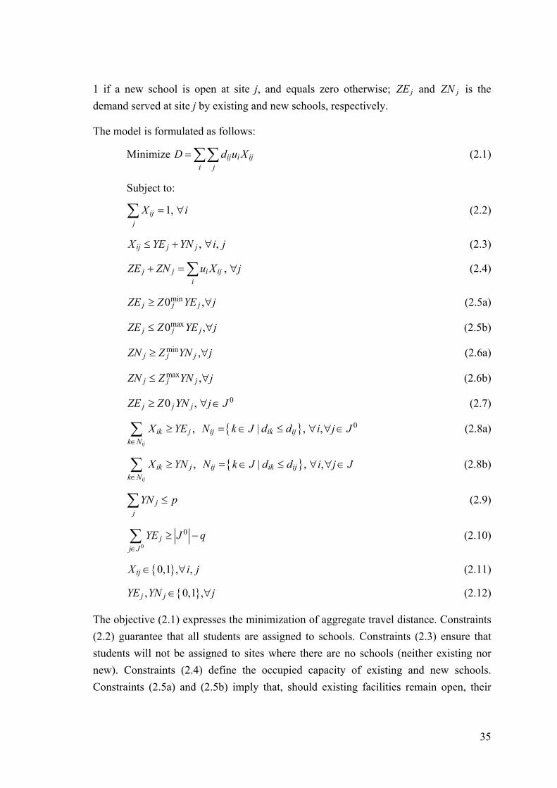
35

1 if a new school is open at site j, and equals zero otherwise; jZE and jZN is the

demand served at site j by existing and new schools, respectively.

The model is formulated as follows:

Minimize ij i iji j

D d u X (2.1)

Subject to:

1ijj

X , i (2.2)

ij j jX YE YN , ,i j (2.3)

j j i iji

ZE ZN u X , j (2.4)

min0j j jZE Z YE , j (2.5a)

max0j j jZE Z YE , j (2.5b)

minj j jZN Z YN , j (2.6a)

maxj j jZN Z YN , j (2.6b)

0j j jZE Z YN , 0j J (2.7)

ij

ik jk N

X YE

, |ij ik ijN k J d d , 0,i j J (2.8a)

ij

ik jk N

X YN

, |ij ik ijN k J d d , ,i j J (2.8b)

jj

YN p (2.9)

0

0j

j J

YE J q

(2.10)

0,1ijX , ,i j (2.11)

, 0,1j jYE YN , j (2.12)

The objective (2.1) expresses the minimization of aggregate travel distance. Constraints

(2.2) guarantee that all students are assigned to schools. Constraints (2.3) ensure that

students will not be assigned to sites where there are no schools (neither existing nor

new). Constraints (2.4) define the occupied capacity of existing and new schools.

Constraints (2.5a) and (2.5b) imply that, should existing facilities remain open, their

36

occupation must satisfy maximum and minimum bounds. Constraints (2.6a) and (2.6b)

define maximum and minimum capacity occupation for new schools. Constraints (2.7)

imply that new capacity can only be added if existing capacity is used ( j jYN YE is

implied, which prevents opening a new school at a site where existing schools were

closed). Constraints (2.8a) and (2.8b) are closest assignment constraints, i.e. they force

students to be served by the closest open school, either existing or new. Constraints

(2.9) and (2.10) bound the number of new schools to be opened and existing schools to

be closed, respectively, where 0J is the current number of sites with schools.

Constraints (2.11) define assignment variables as binary, thus enforcing the single

assignment property, i.e. each population center must be served by only one site.

Constraints (2.12) define location variables as binary.

The differences between the model presented above and the p-median model are as

follows: (i) new facilities can either be open at sites currently with no facilities or be co-

located with an existing facility (in this way, significant capacity expansion can occur,

should it be necessary); (ii) facilities have minimum and maximum capacities; (iii)

single and closest assignment constraints are included (they are redundant in the p-

median model).

The formulation of closest assignment constraints (2.8) was first introduced by Wagner

and Falkson (1975). It has the advantage of remaining valid if a given center has two or

more equidistant sites with open facilities. If this situation does not occur, single

assignment is implied by closest assignment and the integrality constraints (2.11) could

be linearly relaxed. Alternative formulations of closest assignment are analyzed by

Gerrard and Church (1996).

2.5.3 Effect of single and closest assignment

Closest assignment constraints were included in the formulation since, in the presence

of capacity constraints (maximum and/or minimum), optimum solutions do not have the

so-called “closest assignment property”. This means that, in order to minimize total

travel distance or transportation cost, it may not be optimal to assign all demand centers

to the closest open facility. We consider a small example to illustrate the relevance of

this property in the context of public facility planning and to show why it should be

explicitly enforced.

A random instance with 20 population centers was generated to correspond to an

average municipality in Portugal. Centers were uniformly generated in a circle with a 9

km radius. The total number of users was set at 10,000 (10% of a total population of

37

100,000), distributed according to Zipf’s Law with calibration parameter equal to one

(Zipf, 1949; Brakman et al., 2001). Sites are coincident with centers and distances were

computed in kilometers rounded to one decimal place. Minimum capacity was set to

2,000 (thus, the maximum number of facilities is five). In this example there are no

existing facilities.

This instance was solved with three variants of model (2.1)-(2.12): (i) without single

assignment and closest assignment, that is, with the integrality constraints (2.11) relaxed

and constraints (2.8) removed, respectively; (ii) with single assignment only, that is,

with (2.8) removed; (iii) the full model with both sets of constraints. The optimum

solutions are presented in Figure 2.3. Without single and closest assignment (panel i),

the users of some centers are split between several facilities and small centers are served

by distant facilities in order to guarantee minimum capacities. This happens for instance

with the center with 556 users located on the left, which is partly served by the nearest

site with an open facility and two further sites. Even with single assignment (panel ii)

this situation is not eliminated, as the users of small centers might pass near to an open

facility while traveling to the facility to which they are assigned, so that the minimum

capacity of that facility is satisfied. The center with 556 users is now fully served by a

facility in the middle of the region (at the center with 463 users), in spite of a nearby

facility being open (at the center with 2780 users).

Introducing both single and closest assignment constraints eliminates undesirable

configurations of assignments (panel iii). However, the objective function increases by

25% (Table 2.7). Furthermore, in this example, the number of facilities decreases when

closest assignment constraints are added. This can be expected to occur in general

because the number of feasible solutions diminishes. That is, single and closest

assignment constraints prevent disadvantageous assignments of small centers for the

sake of the global optimum. The resulting solutions are easier to interpret and to explain

in a planning context, therefore being more easily accepted by the users.

38

#S

#S

#S

#S

#S

#S

#S

#S

#S

#S

#S

#S

#S

#S#S

#S

#S

#S

#S

#S

#S

#S

#S

#S2780

1390

927

695

556

463

397

347

309278

253

232

214

199

185

174

164

154

146

139

#S

#S

#S

#S

#S

#S

#S

#S

#S

#S

#S

#S

#S

#S#S

#S

#S

#S

#S

#S

#S

#S

#S

#S2780

1390

927

695

556

463

397

347

309278

253

232

214

199

185

174

164

154

146

139 (i) (ii)

#S

#S

#S

#S

#S

#S

#S

#S

#S

#S

#S

#S

#S

#S#S

#S

#S

#S

#S

#S

#S

#S

#S

2780

1390

927

695

556

463

397

347

309278

253

232

214

199

185

174

164

154

146

139 (iii)

Figure 2.3: Solutions with and without single and closest assignment: (i) no assignment constraints,

(ii) single assignment only, (iii) single and closest assignment

Table 2.7: Optimal value and number of facilities with and without single and closest assignment

Model Number of facilities

Aggregate distance (km)

Value Difference to minimum

No assignment constraints 4 14 482.7 0%

Single assignment only 4 16 237.4 12%

Single + Closest assignment 3 18 068.6 25%

CenterCenter + FacilityCenterCenter + Facility

39

2.5.4 Model data

The model of Section 2.5.2 was applied to Coimbra’s secondary schools by considering

the number of students forecast for 2015 and the existing network of public and

subsidized private schools. Students were assumed to be concentrated in 43 centers

(Figure 2.4), corresponding to the 31 communities of the municipality of Coimbra, of

which the five more densely populated were divided into three to four areas each.

Existing schools, as well as possible new schools, were assumed to be located in 43

sites, coincident with the centers. For one particular site (Sé Nova-Combatentes) two

existing schools were aggregated into a single school in the model, since they are

located 500 meters from each other. Distances between centers were measured along the

road network planned for 2015 (Figure 2.4).

#

#

#

#

# ##

#

##

#

#

###

##

#

#

#

#

##

##

###

#

#

###

#

#

#

#

###

#

#

#

Community (1 center)Community (>1 center)

# Population center

#

#

#

#

# ##

#

##

#

#

###

##

#

#

#

#

##

##

###

#

#

###

#

#

#

#

###

#

#

#

Road network# Population center

Figure 2.4: Population centers considered and road network used to compute distances

Minimum and maximum capacity occupation limits are presented in Table 2.8. For new

schools these limits are set by the Ministry of Education. For existing ES schools it was

assumed a minimum of 20 students per classroom, for both public and private schools.

Public schools, which are all of large capacity, should contain at least 18 classes (three

classes per year). For private schools it was assumed that the minimum number of

classes they will offer is six (one class per year).

40

Table 2.8: Capacity and occupation parameters

Type of school

Maximum capacity Minimum occupation

Number of rooms

Students per room

Students Number of

rooms Students per room

Students

New public schools 39 30 1170 18 24 432

Existing public schools current NR 30 - 18 20 360

Existing private schools current NR 30 - 6 20 120

The maximum coverage distance was set to 12.5 km (to ensure travel time is below 30

minutes, at an average speed of 25 km/h by public transportation). This was considered

in the model by setting to zero the assignment variables corresponding to pairs of

centers and sites whose distance exceeded this limit.

2.6 Study Results

In this section, we present the results obtained for Coimbra’s secondary school network

with the model formulated in Section 2.5. Despite its large size (43 centers and sites,

2021 decision variables, of which 1935 are binary, and 5850 constraints), the model was

solved with a commercial optimizer (XPRESS-MP version 2003G; Dash Optimization,

2002). Five alternative solutions were obtained by varying the number of new schools

(parameter p) from zero to four, thus representing different trade-offs between school

accessibility improvements and school network changes. Table 2.9 reports the resulting

number of schools and aggregate accessibility. The chart in Figure 2.5 shows how

aggregate accessibility improves as the number of schools increases. Solutions with less

than two new schools were obtained by removing closest assignment constraints from

the model, otherwise no feasible solutions could be found. It turned out that, in all

solutions, the maximum number of school closures (parameter q) had no influence.

With two or less new schools it is actually desirable to keep all schools open. With more

than two new schools, no feasible solutions could be found without closing one school.

41

Table 2.9: Number of schools and accessibility of model solutions

Number of schools Aggregate distance (km)

New (p) Closed (q) Total Value Difference to

maximum

0 0 11 21 098 0%

1 0 12 14 715 -23%

2 0 13 13 816 -39%

3 1 13 12 518 -48%

4 1 14 10 861 -51%

Note: solutions for p=0 and p=1 do not satisfy closest assignment constraints

0

5000

10000

15000

20000

25000

0 1 2 3 4

Number of new schools

Ag

gre

ga

te d

ista

nce

(km

)

Figure 2.5: Aggregate distance as a function of the number of new schools (p)

School locations and student to school assignments for all solutions are represented in

Figure 2.6. Solutions have the desirable property of being coherent (i.e. when adding

one new school, the previously added schools remain in the same place)7. In the

solution with two new schools (p=2), communities in the southwest of the municipality

travel to a new school located in São Martinho do Bispo because that area of the

municipality does not have enough students to justify a dedicated school there.

Future occupation of schools is summarized in Table 2.10. Public school occupation is

high or at least acceptable (over 60%) in solutions with less than two new schools,

except in the Sé Nova-Combatentes area (where two schools exist). In this area it would

be possible to close one of the existing schools, guaranteeing 80% occupation for the

school remaining open (instead of 40% for both).

7 In chapter 4, the term coherency is employed with a different definition, applying to hierarchical models.

42

Existing School (Open)

Existing School (Closed)

New School

Existing + New School

Population Center

Center-School Assignment

Community

#

#

#

#

##

#

#

##

#

#

###

##

#

#

#

#

#

#

##

##

#

#

#

##

#

#

#

#

#

##

#

#

#

#

%U%U

%U

%U

%U

%U%U%U%U

%U

%U

Souselas

S.P.Frades-Lordemão

Olivais-Vale das Flores

Sé Nova-A.HenriquesSé Nova-Combatentes

Eiras-Pedrulha

São Martinho do Bispo

Santa Clara

CernacheAlmalaguês

Santa Cruz-Conchada

p=0

#

#

#

#

##

#

#

##

#

#

###

##

#

#

#

#

#

#

##

##

#

#

#

##

#

#

#

#

#

##

#

#

#

#

#

#

#

#

##

#

#

##

#

#

###

##

#

#

#

#

#

#

##

##

#

#

#

##

#

#

#

#

#

##

#

#

#

#

%U%U

%U

%U

%U

%U%U

'W

%U%U

%U

%U

São Silvestre

p=1#

#

#

#

##

#

#

##

#

#

###

##

#

#

#

#

#

#

##

##

#

#

#

##

#

#

#

#

#

##

#

#

#

#

#

#

#

#

##

#

#

##

#

#

###

##

#

#

#

#

#

#

##

##

#

#

#

##

#

#

#

#

#

##

#

#

#

#

%U%U

%U

%U

%U

%U'W

'W

%U%U

%U

%U

São Silvestre

São Martinho do Bispo

p=2

#

#

#

#

##

#

#

##

#

#

###

##

#

#

#

#

#

#

##

##

#

#

#

##

#

#

#

#

#

##

#

#

#

#

#

#

#

#

##

#

#

##

#

#

###

##

#

#

#

#

#

#

##

##

#

#

#

##

#

#

#

#

#

##

#

#

#

#

%U%U

%U

%U

%U

'W

%U'W

'W

%U%U

%U

%a

São Silvestre

São Martinho do Bispo

S.P.Frades-Santa Apolónia

Santa Cruz-Conchada

p=3#

#

#

#

##

#

#

##

#

#

###

##

#

#

#

#

#

#

##

##

#

#

#

##

#

#

#

#

#

##

#

#

#

#

#

#

#

#

##

#

#

##

#

#

###

##

#

#

#

#

#

#

##

##

#

#

#

##

#

#

#

#

#

##

#

#

#

#

%U

'W

%U

%U

%U

%U

'W

%U'W

'W

%U%U

%U

%a

São Silvestre

São Martinho do Bispo

S.P.Frades-Santa Apolónia

Santa Cruz-Conchada

Assafarge

p=4

Figure 2.6: Model solutions obtained by varying the number of new schools (p)

43

For two or more new schools occupation is reduced to 40% in the Santa Clara school,

and, for three or more, the school in Santa Cruz-Conchada is closed. Private school

occupation was computed considering the capacity currently allocated to level B2

(which represents about 30% of total ES12 capacity in all schools). This explains the

low occupation (under 40%) of some private schools in some solutions. With less than

two new schools, occupation of existing private schools at S.P.Frades-Lordemão and

São Martinho do Bispo is close to 100%.8

In conclusion, the largest improvement is obtained by adding one school to the current

network. In this scenario, all existing schools guarantee sufficient occupation to remain

open. Adding more schools will bring diminishing returns in terms of aggregate

accessibility.

Table 2.10: Capacity occupation in model solutions

School Status Existing

Capacity

Capacity Occupation (students)

p=4 p=3 p=2 p=1 p=0

Value % Value % Value % Value % Value %

Almalaguês Private 870 199 23 286 33 286 33 286 33 286 33

Assafarge New - 458 - - - - - - - - -

Cernache Private 1620 228 14 599 37 599 37 599 37 599 37

Eiras-Pedrulha Public 1260 1143 91 1029 82 1114 88 1114 88 1224 97

Olivais-Vale das Flores Public 1260 917 73 917 73 917 73 917 73 917 73

S.P.Frades-Lordemão Private 1260 382 30 277 22 582 46 582 46 1215 96

S.P.Frades-S.Apolónia New - 892 - 1111 - - - - - - -

Santa Clara Public 1500 641 43 641 43 626 42 976 65 976 65

São Martinho do Bispo 1 Private 1020 917 90 917 90 917 90 999 98 999 98

São Martinho do Bispo 2 New - 432 - 432 - 432 - - - - -

São Silvestre New - 620 - 620 - 808 - 808 - - -

Sé Nova-A.Henriques Public 1440 1032 72 1032 72 895 62 895 62 895 62

Sé Nova-Combatentes Public 2760 1040 38 1040 38 1040 38 1040 38 1040 38

Souselas Private 1290 369 29 369 29 571 44 571 44 571 44

Santa Cruz-Conchada Public 690 0 0 0 0 483 70 483 70 548 79

8 These results were obtained with non-final data on private school capacity. First, the number of classrooms was estimated by dividing occupation in 2003/04 by 20 students per room (this over-estimated capacity and was revised later in the study). Second, the capacity of modeled private schools, all with both EB12 and ES12 types (considered separately in the models for primary and secondary schools), was assumed to be wholly available for the ES12 type. Later in the study, each of the EB12 and ES12 types was allocated 50% of the total number of classrooms. The new solutions had the same school locations, but some assignments were changed. In particular, some centers assigned to the S.P.Frades-Lordemão school were re-assigned to neighboring schools in scenarios with p<2; the demand of center São Martinho do Bispo, which became higher than the capacity of the school located there, was allowed (by disabling single and closest assignment constraints for this center) to be partly assigned to the neighboring, large school in Santa Clara.

44

2.7 Applying the model with a Geographic Information

System

The study reported in this chapter relied heavily on a Geographic Information System

(GIS) for data handling and result analysis. Geographic data available for the

municipality of Coimbra included community boundaries and population centers,

census tracts, the road network, and existing school locations.

The GIS was used to compute a distance matrix for Coimbra and to display the

solutions obtained with the optimizer (XPRESS-MP) on a map. This was made through

a prototype system based on Arcview GIS version 3.2 (ESRI, 2000). The system

consists of a set of programs implemented with Arcview’s scripting language (Avenue),

and is available from the authors on request. Figure 2.7 shows the steps for applying the

model in practice by using the GIS and the optimizer. Typically, the model is run using

different model parameters (number of schools to open, etc.), and possibly different data

(e.g. school capacities), for analyzing different scenarios.

GIS(Arcview GIS)

Optimizer(XPRESS MP)

Set model parameters (p, q)

Input data:• point shapefile with

centers and sites• line shapefile with road

network

Solve model with optimizer

Prepare model and data files

Display model solution in GIS

All scenarios analyzed

?

End

Output data:• distance matrix

Output data:• optimal solution

Compute distance matrix in GIS

Display model solution (Avenue script)

Solve model

No

Input data:• demand of centers• capacity and location of

existing schools• capacity of new schools• maximum distance of

students to schools

Compute distance matrix (Avenue script)

GIS(Arcview GIS)

Optimizer(XPRESS MP)

Set model parameters (p, q)

Input data:• point shapefile with

centers and sites• line shapefile with road

network

Solve model with optimizer

Prepare model and data files

Display model solution in GIS

All scenarios analyzed

?

End

Output data:• distance matrix

Output data:• optimal solution

Compute distance matrix in GIS

Display model solution (Avenue script)

Solve model

No

Input data:• demand of centers• capacity and location of

existing schools• capacity of new schools• maximum distance of

students to schools

Compute distance matrix (Avenue script)

Figure 2.7: Applying the model by using the GIS and the Optimizer

45

The distance matrix consists of all shortest path lengths between centers and sites and

was computed over the main road network projected for 2015. This road network will

comprise around 1,400 links and 1,000 intersections. The computation was made by

scripting Arcview’s Network Analyst extension, which includes built-in functions for

finding shortest paths on networks. Although computing all shortest paths is an easily

solvable problem (for which there are efficient methods, e.g. Floyd’s algorithm), using a

GIS is still convenient and saves burdensome work. For instance, it is not necessary to

export the road network, which must include nodes for all road intersections, and to

track the correspondence between network nodes and centers or sites.

The display of model solutions on a map largely facilitates the diagnosis of model errors

and the interpretation of model results. Within the prototype system, solutions are

exported from the optimizer as text files and read by a script in the GIS, where they are

displayed as school locations and center assignments. In addition, all solution data (such

as school occupation) can easily be displayed and inspected in tabular form (Figure 2.8).

Figure 2.8: Cartographic solution display and values of non-zero model variables

46

2.8 Conclusion

In this chapter, we presented a study on secondary school planning made within the

framework of Coimbra’s Educational Charter. The main tool used for the study was a

discrete facility location model based on the well-known p-median model. The model

includes constraints on maximum and minimum capacity occupation, single assignment

and closest assignment. Although models containing these ingredients were used before

for other applications, such as the location of health services, the combination of

capacity and assignment constraints had not been reported before in an application to

school network planning. In addition, it was shown that a modern commercial optimizer

is capable of solving models large enough to be useful in practice. The solutions found

through the model clearly suited the needs of a real-world decision-making process

about the future development of a school network, and were extremely helpful in the

discussions held within Coimbra’s Educational Council. This council involves the

municipal administration, school administrations, parents’ organizations and teacher

unions, and is responsible for the approval of the Educational Charter. The multiple

interests of all parties involved, often conflicting, make this decision-making process

complex. The merit of the model presented here is to provide rational solutions as a

basis for discussion. Specifically, it was found that, with only the existing schools, it

cannot be guaranteed that students can be served by the closest school. To accommodate

both the forecast demand and the school typology change (secondary schools will

receive two three-year cycles of education instead of one), the best trade-off between

accessibility improvement and network changes was found to be a single new school.

The study focused on secondary education, for which in Portugal a single type of school

exists. In the near future, a similar study regarding primary education needs to be made.

The model will have to be extended to take into account the existence of two types of

school: EB1 (dedicated to the first cycle) and EB12 (offering the two cycles of primary

education). This leads to a so-called hierarchical facility location model (Narula, 1986),

with two demand levels and two facility levels. Most of previous models (e.g. Weaver

and Church, 1991, and Galvão et al., 2002) do not consider facility capacities. Those

that do (e.g. Eitan et al., 2001, and Galvão et al., 2006) do not include assignment

constraints, such as closest assignment. Our future research will be directed towards the

development of hierarchical models coupling capacity and assignment constraints, and

the development of specialized solution procedures for solving large-scale hierarchical

and non-hierarchical models still out of reach of current state-of-the-art commercial

optimizers.

47

Chapter 3

Application of a hierarchical model to the

location of primary schools

3.1 Introduction

During the last two decades, planning processes involving public facilities such as

schools or hospitals became increasingly more complex, especially because of the

participatory mechanisms they started to involve. Indeed, in the presence of

stakeholders with different viewpoints and interests, planning solutions can only be

widely agreed upon if they are the result of transparent, rational planning processes.

When the number of possible planning solutions is very large, optimization models are

indispensable decision-aid tools. Location models certainly are among the main

optimization models to be used within public facility planning processes. These models

are basically aimed at determining the most efficient locations for all types of facilities

according to some objective or objectives (cost minimization, accessibility

maximization, etc.). They are classified as continuous or discrete depending on whether

the facilities can be located anywhere on the plane or in some points of the plane,

specified in advance. In practical applications, planners often resort to discrete location

models.

Location models have been extensively studied since the 1960s, in the operational

research, management science, industrial engineering, economic geography and spatial

planning literatures. ReVelle and Eiselt (2005) present a concise review of the main

classes of continuous and discrete location models. ReVelle (1987) and Marianov and

Serra (2002) discuss discrete models for public facility location. Daskin (1995) presents

a didactic textbook on modeling and solving discrete location models. Labbé and

Louveaux (1997) review specialized solution methods for basic and extended discrete

location models.

In this chapter, we present a discrete hierarchical location model for public facility

planning, considering several levels of demand and several types of facilities. The

model is an extension of the well-known p-median model, which applies to facility

48

location problems where the objective is to maximize the accessibility of users to

facilities.

The model was developed within the framework of the Coimbra Educational Charter

2006-2015, to help making decisions on the redeployment of the primary school

network of the municipality of Coimbra, Portugal. By law, all Portuguese municipalities

must have an educational charter where the infrastructure, equipment, human, and

financial resources necessary for pre-school, primary and secondary education are

specified. The preparation of the educational charter of a municipality is advised by the

education council of the municipality. This body integrates, among others,

representatives of the local administration, the Ministry of Education, private school

owners, public school administrations, teacher unions, and student parents, which often

have different viewpoints and interests with regard to the evolution of school networks.

This chapter is organized as follows. In Section 2, we present the basic location models

applicable when the objective is to maximize the accessibility of users to facilities.

These models consider a single level of demand and a single type of facility. In Section

3, we discuss different user-to-facility assignment constraints, including a new type of

constraints called path-assignment constraints. In Section 4, we present the hierarchical

location model. In Section 5, we discuss the results obtained with this model for

Coimbra’s primary school network. Finally, in Section 6, we summarize the main

contributions of the chapter, reflect on the application of the model in Coimbra, and

identify some research needs to be fulfilled in the future.

3.2 Basic models

In this section, we present the basic location models upon which the hierarchical model

is built. The simplest of these models is the p-median model (ReVelle and Swain,

1970), which can be stated as follows. We are given a set of demand centers

1,...,I n , where each center i has a demand iu (number of users), a set of sites

1,...,J m , and travel costs ijc for serving all the demand from center i at site j. Travel

costs are defined as ij i ijc u d , where ijd is the unit travel cost between center i and site

j (or distance, if the unit cost is constant). The problem is to find the set of p facilities

that should be open, and to determine which centers should be served from which

facilities, so that the travel costs of serving all the demand from all centers is

minimized. For formulating the model, we define two sets of decision variables: binary

location variables jy , where 1jy if a facility is located (or “open”) at site j J , and

0jy otherwise; and assignment variables ijx representing the fraction of the demand

49

from center i I served at site j J . The formulation of the p-median model is as

follows:

(PM):

Minimize ij iji I j J

c x (3.1)

Subject to: 1ijj J

x

, i I (3.2)

ij jx y , ,i I j J (3.3)

jj J

y p

(3.4)

0 1ijx , ,i I j J (3.5)

{0,1}jy , j J (3.6)

The objective function (3.1) of this mixed-integer optimization model expresses the

minimization of travel costs, which can be seen as a proxy for accessibility

maximization. Constraints (3.2) state that all centers have to be fully served. Constraints

(3.3) link location and assignment decisions by stating that centers can only be assigned

to an open facility. Constraint (3.4) sets the number of open facilities equal to parameter

p. Finally, constraints (3.5) and (3.6) define decision variables.

Optimal solutions of (PM) have the so-called single assignment and closest assignment

properties (Krarup and Pruzan, 1983), that is, centers are fully served by the closest

open facility (or, if travel cost is not monotonically dependent on distance, the least

travel cost facility). This happens because, as there are no capacity constraints, nothing

is gained by splitting the demand from a given center across several facilities, and the

objective forces centers to be assigned to the closest (least cost) facility.

The second basic model is derived from (PM) by adding constraints on the minimum

and maximum capacity of facilities and deleting the constraint on the number of open

facilities. Note that, with the capacity constraints, the number of open facilities becomes

an output of the model rather than a parameter. Let jb and jB be the minimum and

maximum capacity for a facility to be open at site j. This model, denoted capacitated

median model, is formulated as follows:

(CM):

Minimize ij iji I j J

c x (3.7)

50

Subject to: 1ijj J

x

, i I (3.8)

ij jx y , ,i I j J (3.9)

i ij j ji I

u x b y

, j J (3.10)

i ij j ji I

u x B y

, j J (3.11)

| ik ij

ik jk J d d

x y

, ,i I j J (3.12)

0,1ijx , ,i I j J (3.13)

0,1jy , j J (3.14)

Expressions (3.10) and (3.11) are, respectively, the minimum and maximum capacity

constraints. As the closest assignment and single assignment properties of solutions do

not hold for capacitated models, they are enforced explicitly with constraints (3.12) and

(3.13), respectively. Closest assignment constraints (3.12) work as follows. For any

center i and site j, if 0jy then the constraint has no effect; if 1jy then center i must

be fully served from the facility located at site j or from a facility at the same or lower

distance. Gerrard and Church (1996) thoroughly review formulations and applications

of closest assignment constraints in several location models arising in the public and

private sectors. Although the authors note that a different formulation, the so-called

Rojeski-ReVelle (RR) constraints, is frequently used in the literature, we opted for

constraints (3.12) for two reasons. First, unlike RR constraints, constraints (3.12)

remain valid if a given center has two or more equidistant facilities that are the closest.

Second, constraints (3.12) provide a tighter linear relaxation, as RR constraints are

implied by (3.12) together with (3.9); thus, the model can be solved more efficiently

with an integer optimization algorithm based on linear relaxations. Finally, constraints

(3.13) force assignment variables to be binary. We remark that if all centers have a

single closest facility then constraints (3.12) will force assignment variables to be

integer, even if (3.13) is relaxed. Otherwise, if a center has two or more equidistant

facilities that are the closest, constraints (3.12) allow demand to be freely distributed

among those facilities and (3.13) is necessary to impose single assignment.

Unlike the p-median model, the capacitated median model has rarely been dealt with in

the literature. Carreras and Serra (1999) use it without the maximum capacity

constraints to represent a pharmacy location problem in a rural region, and solve it

through a tabu search heuristic. Verter and Lapierre (2002) employ a similar model for

locating preventive health care facilities with the objective of maximizing population

51

coverage, and solve it with a commercial optimizer. Kalcsics et al. (2002) use model

(CM) with constraint (3.4) for designing balanced and compact sales territories, and

solve it through a variable neighborhood search heuristic.

3.3 Assignment constraints

In this section, we analyze the spatial pattern of user-to-facility assignments resulting

from different assignment constraints. As noted previously, solutions to location models

including capacity constraints do not have the single and closest assignment properties.

This may happen because facilities have limited capacity, and thus users are diverted to

other facilities, or users are “captured” to ensure the minimum capacity of a facility. In a

public facility planning context, it should be prevented that users from the same center

are split among different facilities; that users from neighboring centers are assigned to

different facilities; that users are assigned to a distant facility when there are closer open

facilities; that the path traveled by users to the facility they are assigned to crosses a

center assigned to a different facility. If these conditions are violated, solutions are

difficult to interpret by decision-makers and to explain to users, and will certainly be

difficult to implement in practice. Gerrard and Church (1996) make a similar argument

in their article, where they recommend the use of closest assignment constraints in

capacitated location models for public facility planning because they are likely to

improve public confidence in and acceptance of the corresponding solutions.

Our analysis focuses on three types of constraints: the closest assignment constraints

(3.12); the single assignment constraints (3.13); and a new type of constraints

designated as path assignment constraints (3.15). The latter are an alternative to closest

assignment constraints. Although they do not require centers to be assigned to the

closest facility, they guarantee that, if a center is assigned to a given facility, all centers

“near” the “path” traveled by the users to reach the facility must also be assigned to it.

The definition of “near” depends on the context of application of the model. The

formulation of path assignment constraints is as follows:

ij

kj ij ijk P

x P x

, ,i I j J (3.15)

where ijP is the subset of centers k I that are “near” the shortest path from i to j, and

ijP is the cardinality of this set. Expression (3.15) states that if 1ijx then 1kjx for all

ijk P .

Some constraints used in districting models are similar to the path assignment

constraints. These models apply to the partitioning of a set of spatial units (i.e. city

52

blocks, census tracts, or other geographic entities) into subsets, called districts,

according to some objective. Like with location models, spatial units are represented

with discrete centers connected through an underlying network. Desired properties of

districts often include compactness and contiguity, i.e. they should be round shaped

rather than spread out, and should be connected. Kalcsics et al. (2002) use model (CM)

for sales districting, including closest assignment in order to produce connected

districts. Zoltners and Sinha (1983) formulate a model for sales districting, where

district centers (i.e. the seed units for the districts) are predefined. Considering binary

decision variables 1ijx if unit i is assigned to district j, and zero otherwise, contiguity

is enforced with constraints

ij

ij kjk A

x x

, ,i I j J (3.16)

where ijA is the set of units k I that immediately precede unit i on a shortest path from

district center j to unit i. Expression (3.16) states that unit i can be assigned to district j

only if at least another unit, adjacent to i on a path connecting to the district center, is

also assigned to j. In order to reduce the “rigidity” of assignments (as building districts

along shortest paths guarantees contiguity but rules out some contiguous

configurations), the authors propose augmenting sets ijA by either considering the

second, third, etc. shortest paths, or by manual modification by an expert user. A strict

shortest-path approach is adopted by Mehrotra et al. (1998) to ensure contiguity in a

political districting model. Caro et al. (2004) present a model for school districting (with

predefined school locations) including constraints similar to (3.16), where sets ijA are

defined as the set of units k I that are adjacent to unit i and are closer to district center

j than to unit i (but not necessarily on the shortest path).

The impact of including the different assignment constraints in a location model will be

illustrated with one of the random instances used to test model (CM).9 The instances

were built as follows. First, a set of 20n centers was generated uniformly in the unit

square and their coordinates scaled by 1000. Sites were assumed coincident with

centers. Then a planar network was created by computing the Delaunay triangulation

(Weisstein, 1999), with edge length set equal to the Euclidean distance. Distances ijd

were computed by finding all shortest paths on the resulting network. Demands iu were

generated uniformly in the interval 5 to 95. Minimum capacities jb were set to 200 for

all sites. Maximum capacities jB were set to the total demand (i.e. they are not binding). 9 This example partly repeats a similar one in chapter 2, but uses an instance built in a different way, more suitable to illustrate path assignment constraints.

53

Finally, path assignment sets ijP were created by adding all centers in the shortest path

from i to j, plus all centers within a radius of 100 from any node in this path. Panel (i) of

Figure 3.1 shows the network and demands of the test instance. As the total demand is

809, at most four facilities can satisfy the minimum capacity of 200.

This instance was solved with four variants of model (CM): without assignment

constraints, i.e. (3.12) removed and (3.13) relaxed; with single assignment only, i.e.

(3.12) removed; with single+path assignment, i.e. (3.12) replaced by (3.15); and with

single+closest assignment, i.e. the full model (CM). Solutions are shown in Figure 3.1

(where numbers in panels (ii)-(vi) refer to capacity). The p-median model (PM) solution

is included for comparison, with p=4. In this solution, centers are fully assigned to the

closest facility, but one of the facilities does not satisfy the minimum capacity

constraints. On the other hand, all solutions of variants of model (CM) satisfy minimum

capacities, but some undesirable user-to-facility assignments occur if path or closest

assignment constraints are not imposed. Without any assignment constraints, the

demand from some centers is split among two facilities. With single assignment only,

split demands are eliminated but some centers are assigned to a facility much further

than the closest. Adding path or closest assignment constraints eliminates these

undesirable patterns (although with path assignment one of the centers is not assigned to

the closest facility). As expected, adding more constraints degrades the optimal

objective value (Table 3.1). In addition, in this example, solutions with path or closest

assignment constraints have fewer open facilities. This can be expected to occur

frequently because the number of feasible solutions diminishes. That is, path and closest

assignment constraints prevent disadvantageous assignments of some small centers for

the sake of the global optimum. The resulting solutions are easier to interpret and to

explain in a planning context, therefore being more likely to be accepted by the users.

Table 3.1: Solutions for random instance

Model Number of open

facilities Relative objective

value

p-median 4 83%

(CM), no assignment constraints 4 91%

(CM), single assignment only 4 100%

(CM), single+path assignment 3 138%

(CM), single+closest assignment 3 146%

54

#

#

#

# #

#

#

#

#

#

#

#

#

#

#

#

#

#

#

#

#S

#S

#S

#S #S

#S

#S

#S

#S

#S

#S

#S#S

#S

#S

#S

#S

#S

#S

#S

25

52

9

9 59

33

2148

34

86

10

648

66

24

28

16

7880

77

center assigned to closest facility center assigned to non-closest facilitycenter with an open facility center assigned to closest facility center assigned to non-closest facilitycenter with an open facility

#S

#S

#S

#S #S

#S

#S

#S

#S

#S

#S

#S#S

#S

#S

#S

#S

#S

#S

#S

%U

%U%U

%U203

231168

207

#S

#S

#S

#S #S

#S

#S

#S

#S

#S

#S

#S#S

#S

#S

#S

#S

#S

#S

#S

S

S

S%U

%U%U

%U200

209

200

200

#S

#S

#S

#S #S

#S

#S

#S

#S

#S

#S

#S#S

#S

#S

#S

#S

#S

#S

#S

S

S

S

%U

%U%U

%U203

202202

202

#S

#S

#S

#S #S

#S

#S

#S

#S

#S

#S

#S#S

#S

#S

#S

#S

#S

#S

#S

S %U

%U

%U

371

231

207

#S

#S

#S

#S #S

#S

#S

#S

#S

#S

#S

#S#S

#S

#S

#S

#S

#S

#S

#S

%U

%U

%U276

307

226

(i) network and demands (ii) p-median model

(iii) Model (CM), no assignment constraints (iv) Model (CM), single assignment only

(v) Model (CM), single+path assignment (vi) Model (CM), single+closest assignment

Figure 3.1: Solutions for random instance

55

3.4 Hierarchical model

In this section we present a hierarchical version of the capacitated median problem of

Section 2, considering several levels of demand and several types (or levels) of

facilities. Specifically, the demand of centers is discriminated in levels, which must be

separately assigned to facilities capable of providing them. We consider a nested (or

successively inclusive) hierarchy of facilities where a level-s facility (s=1, 2, …, ns) can

serve demands of level 1, …, s. Examples of nested hierarchical facilities arise in the

context of public facility planning. A typical example is a health care network

composed of local health care units, providing basic services, and central hospitals

providing both basic and specialized services. Another example is an education

network, composed of kindergartens, primary schools and secondary schools, in which

a higher level of education can only be located at a site if all lower-levels are also

located there. As noted by Weaver and Church (1991), the various levels of facilities

may or may not be physically distinct (in the example of schools, these could be

separate buildings located in the same community). Other examples of hierarchical

facilities arising in postal and banking services are described by Daskin (1995).

Reviews and classifications of hierarchical models are provided by Narula (1986) and

Church and Eaton (1987), focusing on models with distance minimization and with

coverage maximization objectives, respectively. Before introducing our model, we will

briefly describe some representative examples of hierarchical extensions of the p-

median model. Weaver and Church (1991) formulate a model with a nested facility

hierarchy with any number of levels. The model does not include capacity constraints,

thus an optimal solution can always be found with the single and closest assignment

properties. The model is solved with Lagrangian relaxation combined with an

interchange heuristic, and results are reported for two test networks, with two and three

levels. Galvão et al. (2006) formulate a model with a nested facility hierarchy with

three-levels, addressing a real-world health care application. The model allows service

referrals (that is, a fraction of demand served at a lower-level facility may be referred

directly to a higher-level facility) and includes capacity constraints (however, single-

assignment is not enforced and split assignments can occur). The authors propose a

Lagrangian heuristic to solve the model. Eitan et al. (1991) formulate a model with

nested or more general facility hierarchies (with any number of levels), capacity

constraints, and service referrals. The model is applied to several problems appearing in

the literature and is solved with a commercial integer optimizer.

56

Relatively to hierarchical models in the literature, the model we present here is the first

to combine capacity constraints (minimum and maximum) with assignment constraints

such as closest- or path-assignment (in addition to single-assignment). Consider the

following additional or revised notation for data: 1,...,S ns is the set of demand

levels (and of facility types); uis is level-s demand of center i; Bjs and bjs are the

maximum and minimum capacities of a type-s facility at site j; 0sJ is the set of sites with

existing type-s facilities; sp is the maximum numbers of new type-s facilities to open;

sq is the maximum numbers of existing type-s facilities to close; sD is the maximum

user-to-facility distance for demand level s. Decision variables are defined as follows:

ijsx is the fraction of the level-s demand of center i satisfied by a facility located at site j;

1jsy if a type-s facility is located at j, and equals zero otherwise; jstz is the capacity

occupied with demand level s of a level-t facility located at j. The hierarchical

capacitated median model is formulated as follows:

(HCM):

Minimize ij is ijsi I j J s S

d u x (3.17)

Subject to: 1ijsj J

x

, ,i I s S (3.18)

|

ijs jtt S t s

x y

, , ,i I j J s S (3.19)

|

jst is ijst S t s i I

z u x

, ,j J s S (3.20)

|

jst jt jts S s t

z b y

, ,j J t S (3.21)

|

jst jt jts S s t

z B y

, ,j J t S (3.22)

| ik ij

iks jtk J d d

x y

, , ,i I j J s S , |t S t s (3.23)

0\ s

js sj J J

y p

, s S (3.24)

0

0

s

js s sj J

y J q

, s S (3.25)

0ijsx , , ,i I j J s S | ij sd D (3.26)

0,1ijsx , 0,1jsy , 0jstz , , , ,i I j J s S t S (3.27)

57

Constraints (3.18) ensure that all demands of all levels from all centers are satisfied.

Constraints (3.19) impose that a given level of demand can only be satisfied by a

facility of equal or higher level. Constraints (3.20) define capacity variables jstz by

stating that the demand of each level assigned to a site has to be served by some facility

of equal or higher level located there. Constraints (3.21) and (3.22) impose maximum

and minimum limits on capacity, according to facility type. With this formulation,

capacity is shared by all demand levels. Additional constraints could easily be added to

impose separate capacity limits per demand level, as the model already includes

capacity variables jstz discriminating the demand levels. Note that constraints (3.19) are

redundant for the integer formulation (that is, the same set of integer solutions is

obtained if they are removed), as constraints (3.20) and (3.21) allow a variable ijsx for a

given s S to be non-zero only if there is a variable jty equal to one for some t s .

However, (3.19) are kept in the formulation as they strengthen the linear relaxation.

Closest assignment constraints (3.23) are written separately per demand level and state

that each demand level must be assigned to the closest facility of equal or higher level.

Constraints (3.24) and (3.25) limit the number of new facilities to open and existing

facilities to close. Constraints (3.26) limit the maximum travel distance between centers

and facilities. Finally, constraints (3.27) define decision variables and enforce single

assignment.

Closest assignment constraints (3.23) may be replaced by path assignment constraints,

stated separately per demand level:

ij

kjs ij ijsk P

x P x

, , ,i I j J s S (3.28)

Note that in constraints (3.28) the assignments of different levels are independent, while

in constraints (3.23) the location of higher-level facilities influences lower-level

assignments.

The formulation of model (HCM) given above allows facility co-location, i.e. the

location of different types of facilities at the same site. This can be advantageous to

satisfy maximum capacity constraints. If co-location is not allowed then the following

constraint should be added to the model:

1jtt S

y

, j J (3.29)

In addition, if co-location is not allowed, capacity constraints (3.20)-(3.22) can be

replaced with the following simpler constraints:

58

jt is ijst S s S i I

z u x

, j J (3.30)

jt jt jtz b y , ,j J t S (3.31)

jt jt jtz B y , ,j J t S (3.32)

where constraints (3.30) define variables jtz as the total demand of all levels served at

site j by a type-t facility, and constraints (3.31) and (3.32) impose minimum and

maximum capacities. If (3.30)-(3.32) are used, constraints (3.19) are not redundant for

the integer formulation and are needed to impose the nested facility hierarchy.

3.5 Case study

In this section, we present a study on the redeployment of Coimbra’s primary school

network. Coimbra is a municipality located in the center-littoral region of Portugal with

a population of 150,000 inhabitants (Figure 3.2). The primary school network of the

municipality is composed of 96 schools (Table 3.2).

#

##

##

# #

#

## ##

####

#

##

#### #

##

##

##

##

#

##

#

#

#

#

#

#

#

#

#

#

#

#

#

#

#

#

#

#

#

#

#

#

##

##

#

#

#

#

#

#

#

River Mondego

#

City ofCoimbra

N

0 5 Kilometers

Figure 3.2: Municipality of Coimbra, demand centers and road network

59

Table 3.2: Coimbra’s school network 10

School Type Number of

schools Number of classrooms

Fraction of capacity

Public EB1 (<4 classrooms) 43 90 12%

Public EB1 (4+ classrooms) 28 149 20%

Private EB1 7 49 6%

Public EB12 9 258 34%

Private EB12 9 210 28%

Total 96 756 100%

Most of these schools are public, but there is a significant number of private schools.

Some of them are fully subsidized by the government because they are located in areas

not covered by public schools. There are two types of primary schools: EB1, for the first

cycle of education; and EB12, for the first and the second cycles. The first cycle of

education comprises four years and is attended by children aged 6 to 9. The second

cycle comprises two years and is attended by children aged 10 and 11. The EB1 school

network consists of 78 schools with a total capacity of 288 classrooms (or 7200

students, assuming a maximum of 25 students per classroom). A large number of these

schools has less than four classrooms, which means that students of different years must

share the same classrooms. The EB12 network consists of 18 schools with a total

capacity of 468 classrooms (or 11700 students). Following a period of fast decline in

school age population, in 2004 the total number of enrollments in the primary schools of

the municipality was 10659 students. Since the aggregate capacity of these schools is

18900 students, the aggregate occupation rate of the existing network was 56%.11

10 Table 3.2 differs from Table 2.2 (chapter 2) in some of the data: (i) 15 public EB1 schools with only 1 classroom are excluded (in the next academic year they were to be closed or converted to kindergartens); (ii) private school capacity is measured differently: the number of classrooms was estimated by dividing occupation in 2003/04 by 20 students per room (this over-estimated capacity and was revised later in the study); for schools with both EB12 and ES12 types, each type was allocated 50% of the total number of classrooms. 11 The EB1+EB12 capacity of 18900 differs from EB1+EB23 capacity in Table 2.2 (chapter 2) because the latter uses different private school capacities (as noted before) and includes public EB1 schools with 1 classroom. It also differs from EB1+EB12 capacity in Table 2.5 (chapter 2) because the latter uses different private school capacities and excludes all public EB1 schools with less than 4 classrooms.

The EB1+EB12 current occupation of 56% is not comparable to the EB1 and EB23 occupations higher than 80% in Table 2.3 (chapter 2) because the latter includes demand level B3 (and also uses different private school capacities).

60

The study was made using the hierarchical capacitated median (HCM) model

introduced in the previous section. Applications of location models to school network

planning are numerous and we cite only some representative, relatively recent

examples. Church and Murray (1993) present a multi-objective model considering

school openings and closures and capacity balancing between schools. Pizzolato and

Silva (1997) and Pizzolato et al. (2004) use a p-median model for clustering population

centers. The clusters thus found are then analyzed by confronting total existing school

capacity and population. Antunes and Peeters (2001) develop a dynamic location model

where schools can be opened or closed, and their capacity can be expanded or reduced

over time, with the objective of minimizing total discounted costs. Related models,

where location decisions are not involved, address the short-term school network

management problem of assigning students to existing schools. Church and Schoepfle

(1993) describe a multi-objective model considering student preferences for schools and

balancing of school capacity occupation and racial mix across schools. Caro et al.

(2004) present a model for school districting contemplating several desired properties of

school districts, including capacity balancing and contiguity. As far as we know, no

school network planning study (or other public facility planning study) reported in the

literature relied on a hierarchical model with capacity and assignment constraints.

Three objectives were pursued by the education authorities. First, school capacity

should be adjusted to education demand (as noted above, current aggregate occupation

rate is just 56%). Second, accessibility of students to schools should be maximized.

Third, changes to the existing network should be small, either because of scarce public

budgets to build new schools or to avoid public reactions against school closure

(particularly from parents and teachers). These objectives may of course be conflicting.

With regard to the first objective, following a decision by the education authorities,

existing schools included in the study were current public schools with four classrooms

or more and subsidized private schools. Other private schools, located in areas covered

by public schools, which compete with public schools and are not subsidized, were left

out of the study. Small public EB1 schools with less than four classrooms were also left

out of the study, assuming these will be phased out in favor of larger, better equipped

schools. In aggregate terms, the study included 25 EB1 schools with 4 to 10 classrooms

and 14 EB12 schools with 15 to 36 classrooms, giving a total capacity of 149 and 367

classrooms, respectively.12 As projected demand in 2015 for the two cycles of education 12 The 25 EB1 schools with 4+ classrooms correspond to the 28 in Table 3.2, with 3 pairs of these having been aggregated into a single school in the model since they were located in the same discrete center.

61

is 6300 and 3150 students, the aggregate occupation rate of the resulting school network

would be 73% 13.

The municipality of Coimbra was discretized in 68 population centers (Figure 3.2).

Sites were assumed to be coincident with centers. For this level of aggregation, eight

centers contain both EB12 and EB1 schools. Travel was assumed to be made along the

main road network, which is fully served by public transportation.

Three scenarios for the redeployment of the school network were considered. In

Scenario 1, the minimum occupation of EB1 and EB12 schools was set to 40 and 120

students, respectively, to meet the guidelines of the Ministry of Education for school

capacity (MinEdu, 2000). In Scenario 2, the minimum occupation of schools was

increased to 80 students for EB1 schools and to 75% of current maximum capacity for

EB12 schools. Scenario 3 is the same as Scenario 2, but allowing a new EB12 school to

be opened, with a capacity between 360 and 600 students. The purpose of Scenarios 2

and 3 was to find the best way of adjusting the existing capacity to forecast demand,

while keeping schools with good occupation. The maximum student-to-school travel

distance was set to 8 km in all scenarios, also to meet the guidelines of the Ministry of

Education.

We first solved model (HCM) with closest assignment constraints (3.23). For this

model, no feasible solutions could be found for any one of the three scenarios, as these

constraints are too “rigid” given the spatial distribution of existing capacity versus

forecast demand. Then model (HCM) was used with path assignment constraints (3.28)

replacing (3.23). The computation of data for these constraints was carried out in two

main steps (recall that the path-assignment set ijP for a given center i and site j contains

all centers “near” the travel path between i and j). First, buffers around each center were

created with a radius of half the distance to the nearest neighbor, truncated to a

maximum of 1 km, measured along the road network. Second, all centers whose buffer

is intersected by the shortest path (on the road network) from i to j were added to set ijP .

In the example of Figure 3.3, 38,8 38,36,8P , which means that if center 38 is

assigned to school 8, then center 36 must be assigned to the same school.

13 The EB1+EB12 future occupation of 73% differs from similar data in Table 2.5 (chapter 2) because the latter includes non-subsidized private schools and uses different private school capacities.

62

Figure 3.3: Detail of path assignment

The models were implemented with Dash Optimization’s XPRESS-MP package. The

modeling environment was XPRESS Mosel 1.4 (Dash, 2004) and the solver was

XPRESS Optimizer version 15.30 (Dash, 2005), running under Windows XP on a

computer with a Pentium-M 1.3 GHz CPU and 512 MB of memory. All model runs

took less than three minutes, as in this study the number of schools to open or close is

relatively small. Arcview GIS 3 (ESRI, 2000) was used in conjunction with the

optimizer for data handling and result analysis. Three programs were developed in

Arcview’s scripting language for the following purposes: (i) computing the distance

matrix between all centers using the road network; (ii) computing sets ijP to be used

with path assignment constraints; (iii) importing and displaying the solution output by

the optimizer. The first two make use of Arcview’s Network Analyst extension. In

particular, the practical usefulness of path assignment constraints is closely tied to the

ability to compute data with a real road network, and thus the use of a GIS is

fundamental for this purpose. Church (2002) discusses the link between GIS and the

development and application of location models.

The solutions obtained for the three scenarios are summarized in Table 3.3, where

parameters q1 and p2 are the maximum number of EB1 schools to close and EB12

schools to open, respectively (for all scenarios, no new EB1 schools could be open and

any number of EB12 schools could be closed). The existing school network is sufficient

for the future needs of the municipality (Scenario 1), with around 30% of slack capacity.

Three EB1 schools do not meet the minimum occupation requirements and are closed.

A seemingly awkward assignment occurs for centers 36 and 38 (shown in Figure 3.4,

#

##

#

#

# #

#

## ##

##

#

##

##

###

# ## #

##

##

#

#

#

##

#

#

#

#

#

#

#

%U

%U

%U

%U

%U

%U%U

%U

35

3836

32

8

BuffersRoad networkRoute 38 - 8

# Centres%U Existing EB12 schools

63

expanded in detail in Figure 3.3), which are sent south to center 8. However, the

existing schools at centers 35 and 32 do not have enough capacity, and center 8 is less

than one kilometer further away than those schools. If the minimum occupation is

augmented (Scenario 2), average occupation increases but total travel distance is

degraded by 15%, mainly because of the closure of one EB12 school in the south-east

of the municipality (Figure 3.5). In this scenario, 12 EB1 schools are closed. If a new

school is allowed (Scenario 3), high average occupations are still guaranteed and travel

distance is only 5% higher than in Scenario 1 (Figure 3.6). The main beneficiaries are

centers 36 and 38, located in a fast growth area currently not covered satisfactorily.

Table 3.3: Summary of solutions for the three scenarios 14

Scenario

Model parameters

Total travel distance

Aggregate school occupation

Number of schools

Total New Closed

q1 p2 km Relative EB1 EB12 Total EB1 EB12 EB1 EB12 EB1 EB12

1 3 0 12527 100% 63% 79% 74% 22 14 0 0 3 0

2 Unlim. 0 14391 115% 78% 90% 88% 13 13 0 0 12 1

3 Unlim. 1 13183 105% 75% 87% 85% 12 14 0 1 13 1

14 The model may have alternative optimal solutions with distinct assignments to co-located EB1 and EB12 schools. In scenarios 2 and 3, model solutions were post-processed to give priority to the occupation of EB12 schools: demand was transferred from EB1 schools to co-located EB12 schools while capacity allowed; EB1 schools were closed if all their demand was transferred.

We also note that, in Figure 3.4 and others below, when level-1 assignments are not visible, they coincide with superimposed level-2 assignments.

64

#

#

##

#

## #

#

##

#

#

#

#

#

##

#

# #

# #

##

##

#

#

#

#

#

#

#

#

#

#

#

#

#

#

##

#

## #

#

##

#

#

#

#

#

##

#

# #

# #

##

##

#

#

#

#

#

#

#

#

#

#

#

#

%U

%U

%U

%U

%U%U

%U $T$T

$T

$T

$T$T

$T$T

$T

$T

$T

$T

$T$T

38

36

8

32

#

##

#

#

# #

#

## ##

###

##

##

###

# ## #

# #

##

#

#

#

##

#

#

#

#

#

#

#

#

#

#

#

#

#

#

#

#

#

#

#

#

#

#

##

##

#

#

#

#

#

#

#

%U

%U

%U

%U

%U

%U

%U

%U%U

%U

%U

%U%U %U

$T$T

$T$T

$T

$T

$T

$T

$T$T

$T$T

$T $T

$T

$T

$T$T $T

$T

$T

$T

$T$T $T

# CentresLevel 2 assignmentsLevel 1 assignments

EB12 schools

%U Closed

%U Open

'W New

EB1 schools

$T Closed

$T Open

Figure 3.4: Solution for Scenario 1

#

#

##

#

## #

#

##

#

#

#

#

#

##

#

# #

# #

##

##

#

#

#

#

#

#

#

#

#

#

#

#

%U

%U

%U

%U

%U%U

%U $T$T

$T

$T

$T$T

$T$T

$T

$T

$T

$T

$T$T

#

##

#

#

# #

#

## ##

###

##

##

###

# ## #

# #

##

#

#

#

##

#

#

#

#

#

#

#

#

#

#

#

#

#

#

#

#

#

#

#

#

#

#

##

##

#

#

#

#

#

#

#

%U

%U

%U

%U

%U

%U

%U

%U%U

%U

%U

%U%U %U

$T$T

$T$T

$T

$T

$T

$T

$T$T

$T$T

$T $T

$T

$T

$T$T $T

$T

$T

$T

$T$T $T

# CentresLevel 2 assignmentsLevel 1 assignments

EB12 schools

%U Closed

%U Open

'W New

EB1 schools

$T Closed

$T Open

Figure 3.5: Solution for Scenario 2

65

#

#

##

#

## #

#

##

#

#

#

#

#

##

#

# #

# #

##

##

#

#

#

#

#

#

#

#

#

#

#

#

%U

%U

%U

'W%U

%U%U

%U $T$T

$T

$T

$T$T

$T$T

$T

$T

$T

$T

$T$T

#

##

#

#

# #

#

## ##

###

##

##

###

# ## #

# #

##

#

#

#

##

#

#

#

#

#

#

#

#

#

#

#

#

#

#

#

#

#

#

#

#

#

#

##

##

#

#

#

#

#

#

#

%U

%U

%U

%U

%U

%U

%U

'W %U%U

%U

%U

%U%U %U

$T$T

$T$T

$T

$T

$T

$T

$T$T

$T$T

$T $T

$T

$T

$T$T $T

$T

$T

$T

$T$T $T

# CentresLevel 2 assignmentsLevel 1 assignments

EB12 schools

%U Closed

%U Open

'W New

EB1 schools

$T Closed

$T Open

Figure 3.6: Solution for Scenario 3

3.6 Conclusion

In this chapter, we presented a discrete hierarchical location model for public facility

planning. The main features of the model are: an accessibility-maximization objective;

several levels of demand; several types (or levels) of facilities; a nested hierarchy of

facilities (i.e., a facility of a given level can serve demand of equal and lower levels);

maximum and minimum capacity (or occupation) constraints; and user-to-facility

assignment constraints. The latter include single-assignment and closest-assignment

constraints, as well as a new type of constraints called path-assignment constraints.

They are used to enforce some desirable properties for the spatial pattern of

assignments. The resulting solutions are easier to interpret and to explain in a public

facility planning context, therefore being more likely to be accepted by the users. As far

as the authors know, a model with this set of features has never been dealt with in the

literature.

66

The hierarchical location model was developed to help in a real-world school network

planning process conducted for the municipality of Coimbra, Portugal. At present, most

public planning processes include complex participatory mechanisms. These

mechanisms started to be introduced in the late 80s, as a reaction to the alleged failure

of rational, model-based approaches to public planning (Chadwick, 1978). According to

many planning theorists, a new type of approach was needed focusing on participation

and debate rather than on rationality and modeling (Healey, 1992). This new type of

approach was progressively adopted and now underlies many real-world planning

processes. What we clearly realized from our involvement in the preparation of the

Coimbra Educational Charter is that debate and modeling, instead of being substitutes,

are close complements. Indeed, in the presence of stakeholders with different

viewpoints and interests, like those represented in the education council of the

municipality, objectives can be debated and agreed upon, but solutions that are not

rational for the objectives retained are too fragile to prevail. When the number of

possible solutions is very large, the only way of finding the rational solutions for a

planning problem involves the application of optimization models. Without the

hierarchical location model we developed, it would have been extremely difficult to

arrive at planning solutions widely accepted by the Education Council.

The hierarchical location model was solved with a modern commercial optimizer rather

easily. The use of a GIS package in conjunction with the optimization program was

extremely valuable. In addition to simplify the analysis of results, the GIS was used for

computing data for path assignment constraints, using features such as finding shortest

paths and create buffers, or areas of influence, around centers with distances measured

on the road network. The model was easy to solve because Coimbra, though being one

of the largest municipalities in Portugal outside the metropolitan areas of Lisbon and

Porto, still is a small-size municipality by European standards, and also because small

changes in the number of schools were allowed. If any one of these conditions were not

met, the optimization program would have been unable to do the job. Our future

research will be directed towards the development of specialized solution procedures for

solving large-scale hierarchical and (non-hierarchical) capacitated models with user-to-

facility assignment constraints still out of reach of current modern commercial

optimizers.

67

3.7 Appendix – Path assignment constraints

Introduction

In this appendix, we provide a better formulation of path assignment constraints, and

cite references to previous work using such constraints that came to our attention only

after publishing a journal article based on this chapter.

Alternative formulation of path assignment constraints

In this chapter, path assignment constraints were formulated as follows:

ij

kj ij ijk P

x P x

, ,i I j J (3.15)

This expression states that if 1ijx then 1kjx for all ijk P , where ijP is the subset of

centers k I that are “near” the shortest path from i to j (including i and also j if I = J).

An alternative formulation is as follows:

ij kjx x , , , iji I j J k P (3.15b)

Formulation (3.15b) follows directly from the definition above and it is stronger than

(3.15), which is obtained by summing (3.15b) over all k. Formulation (3.15b) was not

used in the chapter since it apparently requires O(n3) constraints instead of O(n2) as

(3.15). However, on closer analysis, (3.15b) may not actually increase formulation size,

as discussed next.

In expression (3.15b), sets ijP may be replaced by ijP defined as follows, in order to

keep only non-dominated constraints:

\ \ : :ij ij ij ij kj sj ij kj sj ijP P i k P s P P P P P P P s i

Example 1: If I = J and sets ijP are defined by shortest paths on a network, ijP contains a

single node for i j , which is the successor of node i on the path between i and j,

and is empty for i j . For each j J , formulation (3.15b) using sets ijP requires

n-1 constraints, the same as (3.15) (the constraint for i = j is redundant).

Additionally, (3.15b) involves fewer non-zero elements.

Example 2: Consider I = {1,2,3,4} and some j J such that

1 2 {1,2,3,4}j jP P , 3 {3,4}jP , 4 {4}jP , and

1 {2}jP , 2 {1,3}jP , 3 {4}jP , 4 jP .

68

In this example, (3.15b) using sets ijP requires 4 constraints, while (3.15) requires

3 (the one for 4 jP is redundant).

Additional simplifications would be possible with formulation (3.15b). If ij kjP P for

some ,i k I and j J , then it results ij kjx x ; one of the variables is redundant and

can be replaced and removed from the model (this occurs in example 2). When

inequality ij kjx x is added, the variable upper bound constraint ij jx y becomes

redundant and can be removed. Although we do not offer here a preprocessing

procedure to produce a minimal formulation given the sets ijP , we observe that even if

(3.15b) is used with sets ijP instead of ijP , all the simplifications above will likely be

automatically performed by the presolve routines of a generic MIP optimizer.

To summarize, we expect that a location model formulated with constraints (3.15b)

instead of (3.15) is likely to be solved faster with a generic MIP optimizer, since the

formulation is stronger and its size may not increase significantly, or may even

decrease. This is likely to apply even using sets ijP instead of ijP , due to the automatic

simplifications performed by presolve routines.

Previous work using path assignment constraints

It is stated in this chapter that path assignment constraints are a new type of assignment

constraints, since we were unaware of previous work using them (although we cite

related constraints to enforce contiguity in districting models). However, here we cite

references to previous work using exactly the same constraints that came to our

attention only after publishing a journal article based on this chapter.

Shulman and Vachani (1993) and Balakrishnan et al. (1995) study network design

models for local-access telecommunication networks (copper and fiber-optic). These

models consider a set of demand nodes, a tree network connecting nodes to a switching

center, and binary decision variables for locating concentrator on nodes, assigning

nodes to concentrators and expanding capacity on arcs.

Both models include contiguity requirements, stated as follows by Balakrishnan et al.

(1995): “if a concentrator at node j serves node i, then it also serves all other nodes

(including node j) on the path Pij connecting nodes i and j”. The path ijP is unique in

these models, since a tree network is assumed. Nevertheless, given a set of elements ijP ,

this definition is equivalent to the definition of path assignment constraints used in this

chapter.

69

Using the notation of this chapter, contiguity constraints were formulated by Shulman

and Vachani (1993) as:

ij kjx x , , , : iji j k I k P

and by Balakrishnan et al. (1995) as:

ijij k jx x , ,i j I

where kij is the node adjacent to node i on path ijP .

The first formulation is the same as (3.15b) given above, while the second formulation

corresponds to the simplification using the sets ijP defined above when these sets

contain at most one element. Thus, “path assignment constraints” as defined in this

chapter had been proposed before by other authors. However, as far as we know, they

had not been used before in a public facility location model with the paths ijP being

defined as in this chapter (and computed with a GIS) for the purposes discussed in

section 3 of the chapter.

71

Chapter 4

Application of hierarchical models to the

districting and location of courts of justice

4.1 Introduction

Throughout the years, location modeling techniques have been applied to an extremely

wide variety of public facilities (see, for example, Current et al., 2002). However, their

application to one of the most ubiquitous public facilities – courts of justice – is very

rare (and, to the best of our knowledge, has never been described before in a refereed

journal). A possible explanation for this situation is the principle of separation of

powers, which leads governments to avoid interferences with judicial systems (in

democratic countries). However, in Portugal, the judicial system has been going through

a severe crisis and, under the pressure of the public opinion, the government was forced

to take action, launching a vast judicial reform. One of the main constituents of this

reform is a new judiciary map – that is, a new spatial organization for the judicial

system. Indeed, the previously existing map was the result of an evolution with deep

roots in the 19th century. It was based on very small territorial jurisdictions, called

comarcas, which did not favor the specialization of justice. Moreover, in many cases,

the comarcas were not consistent with the jurisdictions of institutions such as local

administration, police, social security, and tax collection, thus contributing to efficiency

losses in the judicial system.

In this chapter, we describe a study made in the University of Coimbra under contract

with the Ministry of Justice of Portugal to define a proposal for the new judiciary map

addressing the following main goals: (1) replace comarcas with larger districts, making

judicial jurisdictions compatible with those of related institutions, and enabling more

effective management of human and material resources; (2) promote the specialization

of the judicial system (through the increase of the number of courts dedicated to specific

litigation types); (3) promote a better balance of supply and demand (judicial litigation);

(4) guarantee a good level of accessibility to courts. For tackling the problems involved

in the accomplishment of these objectives, we developed two optimization models – a

districting model, to determine the borders of new, large judicial districts; and a location

72

model, to determine the location, type, size (measured in number of judges), and

coverage area of the courts included in each new district. The study was carried out in

close cooperation with a task force set up within the Ministry of Justice to accompany

its preparation.

The chapter is organized as follows. We start by describing the context and objectives

of the study, and by presenting the work plan developed to meet these objectives. Next,

we explain how we have determined the reference values used within the study of

judicial litigation and judicial productivity (that is, the number of cases entering and

leaving the courts of justice, respectively). Then, we present the optimization models

developed in the study and describe the results obtained through their application. In the

conclusion, we describe events of the judiciary map reform occurred since the

publication of the study, and summarize the contributions of this chapter.

4.2 Study context

The judicial system of Portugal is seen by many people as one of the country’s greatest

problems. This is the reason why justice was the object of the first and only pact ever

made between the two parties that have alternated in government since the Carnation

Revolution in 1974 – the center-left Socialist Party and the center-right Social

Democratic Party. The pact was signed in September 2006 and involved several issues,

including the reform of the judiciary map as one of the most important.

With respect to this reform, the provisions contained in the pact were the corollary of a

process that started in 2002 when the Government commissioned the Observatório

Permanente da Justiça Portuguesa (OPJP) – a research organization specialized in

judicial affairs – with a study on the spatial organization of the Portuguese judicial

system (OPJP, 2002). After that, many prominent personalities and institutions within

the justice system emitted their opinions on the subject. These opinions were

summarized in a new study of the OPJP released in 2006, where the main problems

faced by the judicial system were plainly identified and the principles to be followed in

the reform of the judiciary map were clearly established (OPJP, 2006). During this

process, many pages of reflections were written. However, six months before the

deadline established in the pact of justice there was still no map: the document

specifying the type, location, size, and coverage area of the courts of justice of Portugal.

One problem identified by the OPJP as being related with the spatial organization of the

justice system was the lack of specialization of courts. The basic courts in Portugal are

the comarca courts, which are generic courts handling all types of cases except the ones

73

for which there is a specialized court with jurisdiction in the area of the comarca.

Before the ongoing reform there were 213 comarcas – and as many comarca courts

(Figure 4.1). Some of the comarca courts (typically the largest ones) had separate civil

and criminal sections, which intervened depending on the nature of the law violations to

process. The specialized courts consisted of labor courts, family and juvenile courts,

civil enforcement courts (dealing essentially with minor debt collection), and commerce

courts. The area of jurisdiction of labor courts covered almost all the country, therefore

comarca courts rarely had to take care of cases involving labor law. The situation was

quite different with respect to the other specialized courts, whose area of jurisdiction is

relatively small. This means that, in large parts of the country, judges in comarca courts

had to deal with a wider variety of cases, and particularly with cases involving the

complex family and commerce laws, with very negative implications for their

productivity.

Generic Labor Family Enforcement Commerce (213) (45) (16) (5) (2)

Figure 4.1: Number and territorial jurisdiction of generic and specialized courts

(mainland Portugal)

A second problem pointed out by the OPJP was the lack of capacity of the courts for

dealing with the increasing volume of litigation observed in the most developed areas of

Portugal. Indeed, in some comarcas of the Littoral (the 50km wide stretch of land

located between the metropolitan areas of Lisbon and Porto), the number of cases

entered in courts was above 1,200 per judge in 2005 (the latest year for which this

information was available when the study was made), when the expected productivity of

a judge is 800 cases per year. The main implication of this has been a steady increase of

the backlog of cases. In contrast, in a large number of comarcas of the Interior (the rest

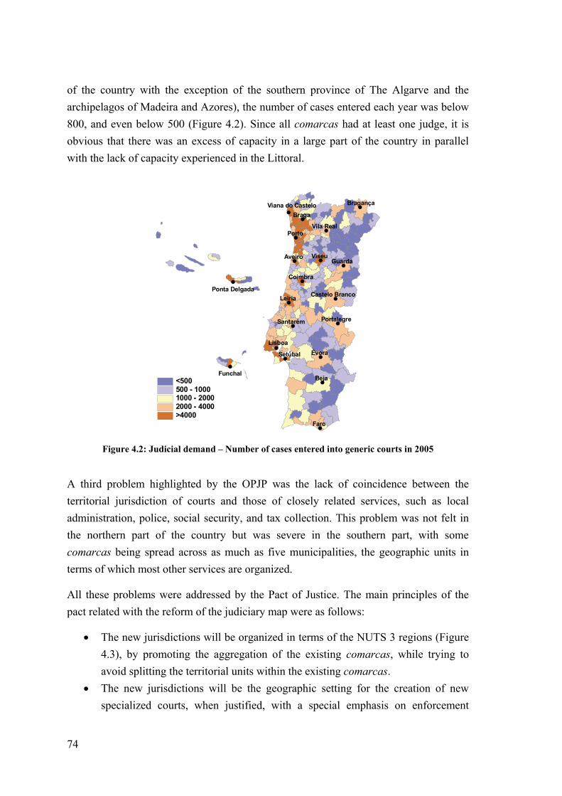
74

of the country with the exception of the southern province of The Algarve and the

archipelagos of Madeira and Azores), the number of cases entered each year was below

800, and even below 500 (Figure 4.2). Since all comarcas had at least one judge, it is

obvious that there was an excess of capacity in a large part of the country in parallel

with the lack of capacity experienced in the Littoral.

##

#

#

##

#

#

# #

#

##

#

#

#

#

#

#

#

Beja

Faro

Braga

Porto

Évora

ViseuAveiroGuarda

Leiria

Lisboa

Coimbra

Setúbal

Bragança

Santarém

Vila Real

Portalegre

Castelo Branco

Viana do Castelo

Ponta Delgada

Funchal<500500 - 10001000 - 20002000 - 4000>4000

Figure 4.2: Judicial demand – Number of cases entered into generic courts in 2005

A third problem highlighted by the OPJP was the lack of coincidence between the

territorial jurisdiction of courts and those of closely related services, such as local

administration, police, social security, and tax collection. This problem was not felt in

the northern part of the country but was severe in the southern part, with some

comarcas being spread across as much as five municipalities, the geographic units in

terms of which most other services are organized.

All these problems were addressed by the Pact of Justice. The main principles of the

pact related with the reform of the judiciary map were as follows:

The new jurisdictions will be organized in terms of the NUTS 3 regions (Figure

4.3), by promoting the aggregation of the existing comarcas, while trying to

avoid splitting the territorial units within the existing comarcas.

The new jurisdictions will be the geographic setting for the creation of new

specialized courts, when justified, with a special emphasis on enforcement

75

courts (the specific reference to these courts reflects the belief that courts of this

type, which had been introduced recently and were still rare in the country,

would greatly help at fighting the slowness of justice).

The new jurisdictions will be the setting for the joint management of human

resources (judges, prosecutors, and other staff) and material resources. Each

jurisdiction will be managed by a judge president and will have a support office

providing technical legal assistance to judges within all courts.

Figure 4.3: NUTS 2 and NUTS 3 regions of Portugal

The problems mentioned above refer to first instance courts. The judicial system of

Portugal is a three-level system. No similar problems were identified with respect to

higher-level courts (the five judicial courts of second instance, with jurisdiction over

NUTS 2 regions, and the Supreme Court of Justice, with jurisdiction over the whole

country), and they were left out of the study. Also out of the study were left the

maritime court and the intellectual property court, because, despite being first instance

courts, their jurisdiction covers the whole country.

AÇORES

MADEIRAAlentejo Central

Alentejo Litoral

Alto Alentejo

Alto Trás-os-Montes

Ave

Baixo Alentejo

Baixo Mondego

Baixo Vouga Beira InteriorNorte

Beira InteriorSul

Cávado

Cova daBeira

Dão-Lafões

Douro

Entre Douroe Vouga

Grande Lisboa

Lezíria doTejo

Médio Tejo

Minho-Lima

Oeste

Península de Setúbal

Pinhal InteriorNorte

Pinhal InteriorSul

Pinhal Litoral

Grande Porto

Serra daEstrela

Tâmega

CENTRO

ALENTEJO

NORTE

ALGARVE

LISBOA

CENTRO

ALENTEJO

NORTE

ALGARVE

LISBOA

76

4.3 Work plan

According to the contract signed with the Ministry of Justice, the development of the

study would involve the following tasks:

1. Clarification of the problem(s) to be solved through the reform of the judiciary

map.

2. Establishment of reference values for judicial litigation (civil, criminal, labor,

etc.) in the reference year of 2015.

3. Establishment of reference values for judicial productivity.

4. Formulation of the optimization model(s) representing the problem(s) to solve.

5. Establishment of the proposal of the judiciary map – one and only one proposal

– based on the solution(s) of the model(s).

6. Analysis of the sensitivity of the proposal to changes in problem definition.

7. Definition of implementation stages for the judiciary map.

The tasks defined are similar to those encountered in many public facility planning

studies: the decision problem to address is properly stated; the demand for service is

estimated; a proposal for the location and size of the facilities that meets the demand is

established based on the solution obtained through an optimization model; a sensitivity

analysis is performed, to better assess the proposal; finally, implementation stages of the

proposal are defined, possibly starting with an experimental stage with limited regional

scale.

The only aspect that we believe deserves a special mention is the fact that there should

one and only one proposal. Our initial idea was that there could be several alternatives

among which to choose. However, the Minister of Justice completely discarded this

possibility saying that: “I do not want any alternatives; we really need to make this

reform. If we propose alternatives, after some time no one really knows what exactly is

being discussed.”

4.4 Problem statement

The aim of the judiciary map proposal is to define the location, type, size (measured in

number of judges), and coverage area (territorial jurisdiction) of first instance judicial

courts in the whole territory of Portugal (mainland and archipelagos of Madeira and

Azores).

The spatial unit adopted both for demand aggregation and for court location was the

municipality, the basic local administration unit in Portugal, of which there are 278 in

77

the mainland plus 30 in the archipelagos. The temporal unit of demand and court

capacity was defined to be one year. The planning horizon was chosen to be the year

2015, which is sufficiently close for judicial litigation to be forecast with acceptable

reliability, but also sufficiently distant for important planned road network expansions

to be completed, according to the National Road Plan 2000, having direct influence on

court accessibility.

The territory is to be partitioned into large districts, each aggregating the jurisdictions of

several existing courts. Within each district, a municipality is selected to become the

seat of the district, based on accessibility and current hierarchical level considerations

(detailed below). The seat’s court, or main court, is the headquarters of the judge

president.

Courts were classified into the following types for the purposes of the study: generic

and specialized of four types – family, labor, enforcement, commerce. Generic courts

serve both civil and criminal cases, as well as other types of cases if a corresponding

specialized court does not exist in the district. Specialized courts serve only cases of the

corresponding type. A fundamental feature of specialization is that if a district has one

or more specialized courts of a given type, then all demand of that type is served at

those courts and not at generic courts.

The following goals were specified, in accordance with the principles defined in the

Pact of Justice: (1) adopt NUTS 3 regions (28 in the mainland plus 2 in the

archipelagos) as the reference for the new districts, keeping municipalities included in

the same old comarcas together in the new districts; (2) create specialized courts in

districts where demand is large enough; (3) promote a better balance of demand and

supply, taking into account given maximum and minimum values of demand per court;

(4) guarantee a good level of accessibility to courts, taking into account a given

maximum travel time to courts.

These goals, together with additional rules for court location and assignment of

municipalities to courts, were translated into a decision problem with the following

decisions, objectives, and constraints.

Decisions:

districting decisions: determine the new districts (municipality-based partitions

of NUTS 3 regions) and select the seat of each district (municipality where the

main court is located);

78

location decisions: determine the location, size, and coverage area for generic

and specialized courts consistent with districting decisions;

Objectives:

1. minimize the number of new districts in each NUTS 3 region;

2. maximize the number of types of specialized courts in the new districts;

3. minimize aggregate travel time to main court weighted by reference litigation;

4. minimize aggregate travel time to generic and specialized courts weighted by

reference litigation;

General constraints:

satisfy all demand (no backlog of cases);

maximum travel time to the main court: 60 minutes;

maximum total number of judges per district: 75, of average productivity;

minimum number of judges in specialized courts: 1, with 80% of the reference

productivity;

minimum number of judges in generic courts: 1, with 50% of the reference

productivity;

Constraints on the location of courts:

main court: is located at a municipality with highest judicial and administrative

hierarchical level, considering the following increasing levels – 0, no existing

court; 1, existing generic court; 2, seat of old judicial circuit (group of old

comarcas); 3, seat of administrative district (group of municipalities); 4, existing

court of second instance;

generic courts: can exist at any municipality with an existing generic court, that

is, no new courts are allowed (however, this does not preclude capacity

expansion of existing courts);

specialized courts: can exist only in municipalities where a generic court is also

located;

enforcement and commerce courts: at most one court of each type can exist per

district, located at the seat of the district;

family and labor courts: one or more courts of each type can exist per district,

located at the seat of the district or at a municipality with an existing specialized

court of either type;

79

Constraints on the assignment of municipalities to courts:

municipalities must be assigned to a single court of each type (i.e. the demand

may not be split among courts located in different municipalities);

municipalities must be assigned to the closest court of each type (in terms of

travel time), with the possible exception of municipalities not having a generic

court, for which the following rules prevail;

municipalities assigned to the same generic court in an old comarca must be

assigned to the same generic court in the future (this rule avoids disaggregating

the old comarcas);

municipalities assigned to the same generic court must also be assigned to the

same specialized courts (this rule establishes coherency between generic and

specialized assignments; coherency is automatically guaranteed for enforcement

and commerce courts, since at most one of each type exists in a district);

a municipality cannot be assigned to family and labor courts located in different

municipalities (this implies family and labor courts must be co-located if both

types exist in a district).

The four objectives above are ordered by priority, that is, each objective was assumed to

be much more important than the next. This allowed the problem to be decomposed into

two sequential sub-problems:

a districting sub-problem, considering only the districting decisions and the first

three objectives;

a location sub-problem, considering only the location decisions and the fourth

objective.

This decomposition into sub-problems is further discussed in section 4.7.3, after

presenting model formulations.

Finally, we remark that location decisions considered that at most one generic court

exists per municipality, and that specialized courts of each type are co-located with

generic courts. In reality, depending on jurisdiction size and existing infrastructure,

generic courts may either be a single unit or be subdivided into specialized civil and

criminal sections, located in the same or distinct buildings; and specialized courts may

be located in a single building together with a generic court or in distinct buildings.

However, the subdivision of generic courts and the precise location of buildings where

courts should be installed within a municipality were left outside the scope of the study.

80

4.5 Judicial litigation

Reference values for judicial litigation (measured in number of cases per year) were

forecast to 2015 using the following method: (1) Stepwise regression of litigation rate

against demographic, employment, and educational variables (using 2001 data); (2)

Selection of the best regression equation; (3) Computation of forecasts for the litigation

rate (from a forecast of the independent variables); (4) Application of litigation rate

forecasts to population forecasts.

Regression models

The following regression models were tested:

1 1 2 2 3 3n A A AL P P P

1 1 2 2 3 3n E E EL P P P

1 1 2 2 3 3n H H HL P P P

Ln: litigation rate of type n (cases per thousand inhabitants); PA1, PA2, PA3:

difference from the national average of the percentage of active resident

population (employed or unemployed) in the primary, secondary and tertiary

sectors, respectively; PE1, PE2, PE3: difference from the national average of the

percentage of persons employed in the primary, secondary and tertiary sectors,

respectively; PH1, PH2, PH3: difference from the national average of the percentage

of resident population per education level: first level of primary education or less,

intermediate level, secondary education or higher, respectively.

The best regression models, obtained through forward stepwise regression (see e.g.

Draper and Smith, 1998) considering parameters as statistically significant when

absolute t values were higher than 2, were as follows:

2130.52 0.82 0.249civil HL P R

21 311.25 0.18 0.19 0.291criminal H HL P P R

233.54 0.17 0.216family HL P R

22 36.08 0.28 0.22 0.286labor A AL P P R

We observe that the explanatory power of these models is low (R2<0.30). Some

attempts were made to improve them, such as an analysis of the spatial pattern of

81

litigation rates (distinguishing north vs. south, littoral vs. interior, low vs. high

administrative hierarchical level), but no patterns could be observed and thus no spatial

dummy variables were included in the models. As we had anticipated, litigation is a

complex phenomenon that would be difficult to model. In spite of this, the regression

coefficients have the expected signs: litigation is higher for higher education levels (this

reflects increased access to justice, since higher educated citizens tend to be better

informed and have higher incomes, and also increased litigation in more complex

economic activities, which tend to require higher educated workers); litigation is higher

for higher weights of the secondary and tertiary sectors (this reflects increased litigation

in more complex economic activities). Thus we decided to retain the regression models

above for litigation forecasts, though aware that the forecast would not be very accurate.

Population forecasts

The reference value of population in 2015 was obtained with the following method.

First, the population forecasts of the National Statistics Institute for NUTS 2 regions

(INE, 2004) were used. Second, regional population growth was distributed by its

constituent municipalities according to three scenarios: (1) proportionally to the

population growth in 1991-2001 (the two last census years); (2) proportionally to the

natural growth rate (births-deaths) in 2004 (the last year of available data); (3)

proportionally to the population in 2001 (the last census year). The three scenarios favor

municipalities with different demographics and dynamics: respectively, high recent

growth, young population, large municipalities with recent population decrease. Finally,

the population in each municipality was taken to be the maximum of all scenarios. This

method produces an over-estimation of total population. However, even with this

optimistic forecast a generalized decrease in the number of generic courts could be

expected, provoking a negative reaction in the affected municipalities. The method

chosen was expected to reduce claims that particular municipalities were treated

unfairly due to the choice of a particular forecast method.

Regarding the projection of independent variables, the percentage of active population

per economic sector was assumed to vary proportionally to the variation in 1991-2001

(a general increase in the tertiary sector was observed, accompanied by a general

decrease in the primary sector and, in some cases, also in the secondary sector). The

percentage of population per education level was also assumed to vary proportionally to

the variation in 1991-2001 (a general decrease in the lower level and an increase in the

higher levels was observed). According to the regression models adopted, these trends

will produce an increase in litigation.

82

Litigation forecasts

In spite of the simplicity of the litigation forecast method, the results were judged to be

credible when data for particular municipalities were analyzed for the years 2001 (the

base year for the forecast), 2005 (the last year of available data, used for control) and

2015 (the forecast year).

A summary of the litigation forecasts is presented in Table 4.1, representing in 2015 a

total of about 770,000 cases of the following types: civil 59% (including enforcement

and commerce); criminal 24%; family 9%; labor 8%.

The significant increase in criminal and family litigation can be attributed to expected

increases in education levels (as well as to the optimistic population forecast), while the

decrease in labor litigation can be attributed to the significant decrease of weight of the

secondary sector expected in a large proportion of municipalities.

Table 4.1: Results of litigation forecasts – number of cases per municipality

Type of case

Civil Criminal Family Labor Total

Total 2001 414 838 104 768 42 875 67 316 629 797

Total 2015 453 963 185 151 70 309 62 582 772 005

Var. 2001-2015 9% 77% 64% -7% 23%

Minimum 2015 22 7 5 5 39

Median 2015 594 227 75 85 995

Average 2015 1 474 601 228 203 2 507

Maximum 2015 48 075 21 262 8 807 5 852 83 996

Civil cases are divided into declarative, commerce and enforcement cases. The

proportions of enforcement and commerce cases in 2005 were 60.0% and 1.4%,

respectively, and were assumed to remain unchanged in the future and to apply to all

municipalities. To account for recently introduced legislation that will tend to decrease

litigation in courts (e.g. decriminalization of some infractions; possibility of extra-

judicial settlements), litigation rates for all case types were multiplied by a factor of 0.9.

4.6 Judicial productivity

Reference values for judicial productivity (number of finished cases per judge in one

year, applying to any judge) adopted in the study for 2015 were as follows:

Global productivity (average for all courts in a district, combining all court types

and case types): 800 cases;

83

Generic court: 800 cases if the court receives enforcement cases; 550 cases

otherwise;

Enforcement court: 2750 cases;

Family court: 800 cases;

Labor court: 950 cases;

Commerce court: 400 cases.

For specialized courts, the values above are approximately the national averages

observed in 2005, and are within the reference productivity intervals used by the

Supreme Judicial Council in the assessment of judges (according to information

provided by the Ministry of Justice). For enforcement courts the middle point of this

interval was adopted, rather than the observed average, since some of these courts had

been installed only recently and the applicable law had been subject to recent changes.

For generic courts, the productivity of 800 is approximately the national average

observed in 2005 (the observed global productivity is similar and the reference value

was assumed to be equal). A lower productivity is considered if the generic court does

not receive enforcement cases, which are generally simpler to judge, but no other

discrimination is made regarding the mix and proportions of case types.

The latter option resulted from an analysis of productivity of judges in generic courts

carried out within the study, using the following regression model:

1 1 2 2 3 3 4 5 6 7 8d ecivil civil criminal family laborF J J J T T T T T

F: number of finished cases per judge; J1, J2, J3: difference from the national

average of the percentage of judges with less than 3 years, between 3 and 6 years,

and more than 6 years of experience, respectively; Tn: difference from the national

average of the percentage of cases of type n (civil cases were divided into

declarative, civild, and enforcement, civile, and commerce cases were excluded

from the analysis).

The best regression model, obtained by forward stepwise regression and using 2005

data only from generic courts under demand pressure (where the number of new cases is

not smaller than the number of finished cases), was the following:

21819.63 2.83 6.61 0.290

ecivilF J T R

As before, the explanatory power is low. Indeed, judicial productivity was expected to

be difficult to capture in a model. Nevertheless, we considered the model to be useful,

84

since the regression coefficients have the expected signs: productivity is lower in courts

with higher proportion of younger judges and higher in courts with higher proportion of

enforcement cases. According to this model, a court not receiving enforcement cases

has a productivity of 543 cases per judge, while one in which all civil cases are

enforcement cases has a productivity of 1205 (smaller than the 2750 assumed above for

a specialized enforcement court). Coefficients of variables related to other case types

were not retained in the model, i.e. other case types had no statistically significant effect

on productivity.

4.7 Optimization models

4.7.1 Literature overview

We now briefly overview the relevant literature before introducing the formulations of

the two optimization models developed in the study. The models presented here are

discrete facility location models, which assume a discrete set of centers where demand

is concentrated and a discrete set of sites where facilities can be located. ReVelle and

Eiselt (2005) and Current et al. (2002) provide general reviews, and ReVelle (1987) and

Marianov and Serra (2002) provide reviews focusing on public sector applications.

Basic models

The models we developed are extensions of a basic model that aims to locate facilities

and assign demand centers to those facilities so that the total demand-weighted

assignment distance is minimized, each center is fully assigned to the closest facility (or

one of the closest, if several are equidistant), and the demand served by each facility

satisfies given minimum and maximum capacities.

This model is called the capacitated median model (CM) by Teixeira and Antunes

(2008), due to its relationship with the classic p-median model (PM), in which facility

capacities are not imposed and the number of facilities is a parameter (p). In the PM

model, solutions naturally have the so-called single and closest assignment properties,

i.e. each center is fully assigned to the closest facility. In the CM model, facility

capacities are imposed: a minimum capacity, representing a threshold to guarantee

economic feasibility of individual facilities or to guarantee increased productivity

through specialization of labor; and a maximum capacity, representing limited space

availability or a threshold to avoid diseconomies of scale. The minimum and maximum

capacities have two consequences: i) they imply, respectively, upper and lower bounds

on the number of facilities, which becomes a model output rather than a parameter; ii)

85

the single and closest assignment properties, if required, must be imposed through

explicit constraints. The single and closest assignment properties are desirable in a

public facility planning context where users are assumed to distinguish locations

through their accessibility, by preferring the closest facility. Hanjoul and Peeters (1987)

further discuss the representation of user preferences in a location model. Teixeira and

Antunes (2008) compare spatial patterns of user-to-facility assignments between the PM

and CM models.

The CM model, unlike the PM model, has rarely been dealt with in the literature.

Carreras and Serra (1999) use it in a pharmacy location problem, and solve it through a

tabu search heuristic. Kalcsics et al. (2002) use it together with a constraint on the

number of facilities for designing balanced and compact sales territories, and solve it

with a variable neighborhood search heuristic. Teixeira et al. (2007) apply it to the

reorganization of a secondary school network, and solve it with a commercial optimizer.

Bigotte and Antunes (2007) present several heuristics to solve the CM model. Related

models have been proposed that do not require all demand centers to be served, but

otherwise combine minimum capacity and closest assignment constraints. Verter and

Lapierre (2002) present a model for locating preventive health care facilities with the

objective of maximizing population coverage, and solve it with a commercial optimizer.

Smith et al. (2009) present a model for locating primary health care facilities with the

objective of maximizing the number of open facilities, and solve it with a commercial

optimizer.

Hierarchical models

Teixeira and Antunes (2008) present a hierarchical version of the capacitated median

model, considering demand for multiple services and multiple facility types, both

classified into n levels, where facilities have a nested service hierarchy: a level n facility

can serve level n demand and all lower levels. An application to the reorganization of a

primary school network with two levels is presented, in which the model is solved with

a commercial optimizer.

The two models presented here are also multiple-service hierarchical extensions of the

capacitated median model. Both models consider two levels of facilities, generic (level

1) and specialized (level 2), organized into a nested hierarchy: level-2 facilities can only

be installed at locations where level-1 facilities also exist. Hierarchical location models,

dealing with the location of multiple facility types, are reviewed by Narula (1986),

Church and Eaton (1987), and Sahin and Sural (2007).

86

Relatively to hierarchical models in the literature, the court location model presented

here (the second model below) is the first to include so-called coherent assignment

constraints together with capacity constraints and closest assignment constraints.

Assignments are said to be coherent if all centers assigned to a given level-1 facility are

assigned to the same level-2 facility. Explicit constraints enforcing coherency were first

introduced by Serra and ReVelle (1993) for a model with two facility types and two

service levels. Other models with the property of coherent assignment are cited in the

survey by Sahin and Sural (2007).

Districting models

We also refer to the related literature on districting models – see e.g. the review by

Kalcsics et al. (2005). Districting models have the purpose of partitioning of a set of

spatial units (i.e. city blocks, census tracts, or other geographic entities) into subsets,

called districts, according to some objective. As in discrete models for facility location,

spatial units are represented with discrete centers connected through an underlying

network. Desired properties of districts often include compactness and contiguity, i.e.

they should be round shaped rather than spread out, and should be connected. The

capacitated median model, when applied to districting problems, tends to produce

districts with these properties, as noted by Kalcsics et al. (2002), who use this model for

designing sales territories: compact districts are promoted by the objective of

minimizing aggregate travel time together with the closest assignment constraints; also,

closest assignment constraints tend to produce connected catchment areas. However, it

should be noted that contiguity is not guaranteed and will depend on the data of

particular instances. In the application described here, contiguity was always observed.

In other cases, specific constraints enforcing contiguity may be required, such as those

reviewed by Duque et al. (2011).

Applications to the justice sector

As far as we know, no previous applications of optimization models for the location of

courts of justice were described or cited in refereed journals. However, there is at least

one such application. Rømo and Sætermo (2000) report on a project of the research

center SINTEF in which a discrete location model was developed for defining the

location and districts of first instance courts in Norway, under contract with the

Ministry of Justice. The model, which was implemented with XPRESS-MP and

embedded into a decision support system, is an extension of the p-median model. The

objective is to minimize total travel distance (optionally to minimize the total

infrastructure and travel costs) subject to a number of courts to be located, a minimum

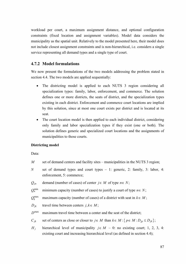
87

workload per court, a maximum assignment distance, and optional configuration

constraints (fixed location and assignment variables). Model data considers the

municipality as the spatial unit. Relatively to the model presented here, their model does

not include closest assignment constraints and is non-hierarchical, i.e. considers a single

service representing all demand types and a single type of court.

4.7.2 Model formulations

We now present the formulations of the two models addressing the problem stated in

section 4.4. The two models are applied sequentially:

The districting model is applied to each NUTS 3 region considering all

specialization types: family, labor, enforcement, and commerce. The solution

defines one or more districts, the seats of district, and the specialization types

existing in each district. Enforcement and commerce court locations are implied

by this solution, since at most one court exists per district and is located at its

seat.

The court location model is then applied to each individual district, considering

only family and labor specialization types if they exist (one or both). The

solution defines generic and specialized court locations and the assignments of

municipalities to those courts.

Districting model

Data:

M set of demand centers and facility sites – municipalities in the NUTS 3 region;

N set of demand types and court types – 1: generic, 2: family, 3: labor, 4:

enforcement, 5: commerce;

jnQ demand (number of cases) of center j M of type n N ;

minnQ minimum capacity (number of cases) to justify a court of type n N ;

maxkQ maximum capacity (number of cases) of a district with seat in k M ;

jkD travel time between centers ,j k M ;

maxD maximum travel time between a center and the seat of the district;

jkC set of centers as close or closer to j M than k M : : jp jkp M D D ;

jH hierarchical level of municipality j M – 0: no existing court; 1, 2, 3, 4:

existing court and increasing hierarchical level (as defined in section 4.4);

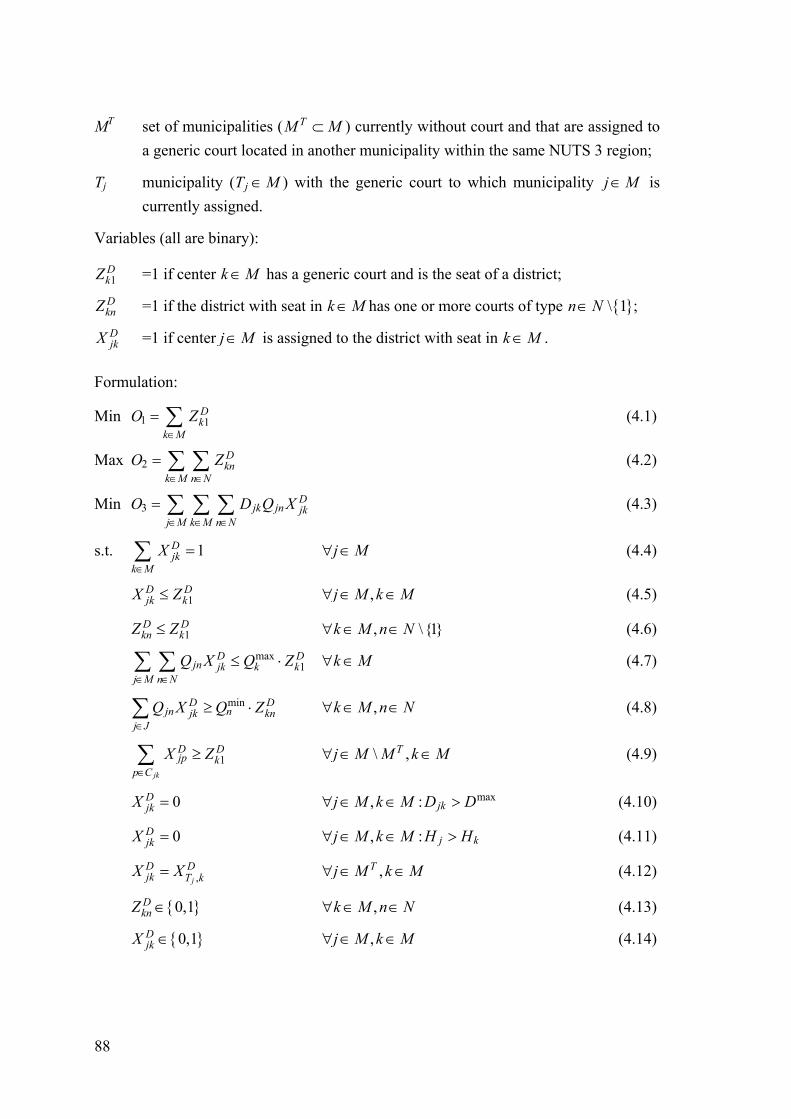
88

MT set of municipalities ( TM M ) currently without court and that are assigned to

a generic court located in another municipality within the same NUTS 3 region;

Tj municipality ( jT M ) with the generic court to which municipality j M is

currently assigned.

Variables (all are binary):

1DkZ =1 if center k M has a generic court and is the seat of a district;

DknZ =1 if the district with seat in k M has one or more courts of type \ 1n N ;

DjkX =1 if center j M is assigned to the district with seat in k M .

Formulation:

Min 1 1Dk

k M

O Z

(4.1)

Max 2Dkn

k M n N

O Z

(4.2)

Min 3D

jk jn jkj M k M n N

O D Q X

(4.3)

s.t. 1Djk

k M

X

j M (4.4)

1D Djk kX Z ,j M k M (4.5)

1D Dkn kZ Z , \{1}k M n N (4.6)

max1

D Djn jk k k

j M n N

Q X Q Z

k M (4.7)

minD Djn njk kn

j J

Q X Q Z

,k M n N (4.8)

1jk

D Djp k

p C

X Z

\ ,Tj M M k M (4.9)

0DjkX , :j M k M max

jkD D (4.10)

0DjkX , :j M k M j kH H (4.11)

,j

D Djk T kX X ,Tj M k M (4.12)

0,1DknZ ,k M n N (4.13)

0,1DjkX ,j M k M (4.14)

89

The objectives (4.1), (4.2), (4.3) are respectively: to minimize the number of districts; to

maximize the number of court types existing in districts; to minimize the total travel

time between centers and seats of district, weighted by the demand of all types.

A lexicographic ordering of objectives was assumed, that is, (4.1) is infinitely more

preferable than (4.2), which in turn is infinitely more preferable than (4.3). Since O1 and

O2 are positive integers, the three objectives were replaced by the following single

objective (where M1 and M2 are suitable large positive constants satisfying M2>O3 and

M1>M2O2+O3 for all values of parameters and variables):

Min 1 1 2 2 3M O M O O

The constraints (4.4)-(4.14) have the following meaning: (4.4) requires each center to be

assigned to one district; (4.5) links the assignment and location variables through the

standard strong formulation (it states that an assignment can only be made to a center

defined as seat of district); (4.6) associates specialized courts (n>1) existing in a district

with the center defined as seat of that district (n=1); (4.7) are maximum capacity

constraints, stated for the total demand of all types in a district; (4.8) are minimum

capacity constraints, stated separately for each demand and court type in a district; (4.9)

are closest assignment constraints; they state that if center k is a seat of district, then any

center j has to be assigned to a seat of district as close or closer than k; these constraints

do not apply to centers in set MT; (4.10) defines the maximum travel time to the seat of

district; (4.11) forbids the assignment of a center to a seat of district with lower

hierarchical level in the current organization (i.e. the seat is chosen among the

municipalities with currently highest hierarchical level); (4.12) guarantees that centers

belonging to the same old comarca have to be assigned to the same new district (i.e. old

comarcas are not disaggregated); finally, (4.13) and (4.14) define all variables as binary.

We note that (4.11) and (4.12) are special purpose constraints imposing that the

reorganization has to take into account the current organization of courts. These

constraints, and also (4.10), lead to a reduction of the effective model size, performed

automatically by the presolve routines of a MIP optimizer.

Location model

Note: The notation M, N, jnQ , minnQ is retained from the previous model, but data is

redefined, as described below and in the next section.

90

Data:

M set of demand centers and facility sites – municipalities in the district;

N set of demand types and court types – 1: generic, 2: family, 3: labor (types 2 and

3 are only included if they exist in the district);

jnQ demand (number of cases) of center j M of type n N ;

minnQ minimum capacity (number of cases) to justify a court of type n N ;

kE =1 if a specialized court (of any type n>1) currently exists at center k M , or

zero otherwise;

jH , jkD , maxD , jkC , TM , jT have the same definitions as in the previous model.

Variables (all are binary):

knZ =1 if a court of type n N is installed in center k M ;

jknX =1 if center j M is assigned to a court located in center k M for demand

type n N .

Formulation:

Min jk jn jknj M k M n N

D Q X (4.15)

s.t. 1jknk C

X

j M ,n N (4.16)

knjknX Z ,j M k M ,n N (4.17)

1kn kZ Z k M , \{1}n N (4.18)

minjn n knjkn

j M

Q X Q Z

k M ,n N (4.19)

11jk

kjpp C

X Z

\ ,Tj M M k M (4.20)

11jk

j jpn knp C

Z X Z

,j M k M , \{1}n N (4.21)

1 1 jpnjk kpnX X X , ,j M k M p M , \{1}n N (4.22)

0jknX , , :j M k M n N maxjkD D (4.23)

2 3jk jkX X ,j M k M , if 3N (4.24)

2 3k kZ Z k M , if 3N (4.25)

91

1 0jkX , :j M k M j kH H (4.26)

, ,jjkn T k nX X ,Tj M M k M ,n N (4.27)

1 0kZ : 0kk M H (4.28)

0knZ 1, \{1}: 0 0Dkkk M n N Z E (4.29)

0,1knZ k M ,n N (4.30)

0,1jknX ,j M k M ,n N (4.31)

The objective (4.15) is to minimize the total travel time between centers and courts,

weighted by demand. Travel times for generic demand (n=1) and for specialized

demand (n>1) are assumed to be commensurable and are given the same weight.

The constraints (4.16)-(4.31) have the following meaning: (4.16) requires each demand

type of each center to be assigned to one court of the corresponding type; (4.17) links

the assignment and location variables of each type (they state that an assignment can

only be made to a center where a court of the corresponding type is located); (4.18)

states that specialized courts (n>1) can only be located in centers where a generic court

(n=1) is also located (this constraint enforces the nested hierarchy); (4.19) are minimum

capacity constraints for each court type; (4.20) are closest assignment constraints for

generic courts; they do not apply to centers in set MT, i.e. without an existing court;

(4.21) are closest assignment constraints for each specialized type, applying only to

centers j where a generic court exists (Zj1=1); if no court exists (Zj1=0) the constraint has

no effect (the inequality is satisfied, irrespective of the values of all other variables) and

the assignment will be determined only by coherency and other constraints; (4.22) are

coherency constraints for each specialized type, stating that if a center j is assigned to a

generic court at k (Xjk1=1) and center k is itself assigned to a specialized court at p

(Xkpn=1), then center j must also be assigned to the specialized court at p (Xjpn=1); (4.23)

defines the maximum travel time to a court; (4.24) implies that each center must be

assigned to family and labor courts located in the same municipality, if both types exist

(|N|=3); (4.25) implies that family and labor courts have to be co-located, if both types

exist; (4.26) forbids the assignment of a center to a court in a municipality with lower

hierarchical level in the current organization; (4.27) guarantees that centers belonging to

the same old comarca have to be assigned to the same courts of each type; (4.28)

forbids opening a new generic court in municipalities where no court currently exists;

(4.29) states that specialized courts cannot be located in municipalities which are not the

seat of the district and where no specialized court of any type currently exists; finally,

(4.30) and (4.31) define all variables as binary.

92

Constraints on the maximum capacity of courts are not imposed explicitly since the

individual courts are assumed to have the same capacity limit as the main court in the

seat of the district, and this limit is guaranteed by the first model.

Regarding the combination of assignment constraints, centers where a level 1 facility is

not installed are subject to coherent assignment but not to closest assignment constraints

for level 2 assignments, through the term (1-Zj1) in (4.21). This was a planning

assumption in the present application. If that term was removed the model would

remain consistent, but the feasible spatial configurations of solutions would be reduced.

We now comment on particular cases of the model, depending on the number of

specialized court types that result from the districting model:

If no specialized types exist (N={1}), a reduced model is obtained, dedicated to

a single (generic) demand and court type; in particular, the following constraints

are excluded: (4.18), (4.21), (4.22), (4.24), (4.25), (4.29).

If both family and labor specializations exist (N={1,2,3}), the two types are not

independent, due to the presence of constraints (4.24) and (4.25). These are

included since, in the present application, centers cannot be assigned to family

and labor courts in different municipalities, which in turn implies the co-location

of family and labor courts (we note that it would suffice to add (4.24), because

(4.25) are implied by the former together with (4.17), (4.19) and the binary

constraints). These constraints effectively reduce assignment and location

decisions to two types – generic (type 1) and specialized (type 2, representing

both family and labor). The formulation could thus be simplified, retaining only

the variables and constraints for a single specialized type, except for minimum

capacity constraints (4.19), which must still be stated separately for each

specialized subtype (that is, family and labor courts must be co-located, but each

type must separately guarantee its minimum capacity). However, we opted to

keep the general formulation above, which can address other applications where

constraints (4.24) and (4.25) do not apply. Additionally, there is no

computational burden, since the model will be automatically simplified as

described above by the presolve routines of a MIP optimizer.

Similarly to the first model, (4.26)-(4.29) are special purpose constraints imposing that

the reorganization has to take into account the current organization of courts. These

constraints, together with (4.23) and, as noted above, (4.24)-(4.25), lead to a reduction

93

of the effective model size, performed automatically by the presolve routines of a MIP

optimizer.

Alternative formulations of closest assignment constraints have been proposed in the

literature – see Gerrard and Church (1996) and Hansen et al. (2004). The latter authors

show that formulation (4.20) provides a tighter linear programming relaxation than the

alternatives discussed. The formulation of coherency constraints (4.22) is equivalent to

the one proposed by Serra and ReVelle (1996).

Finally, we observe that both models above are hierarchical extensions of the basic,

single-service capacitated median model. The first model (districting) is a

straightforward extension, since it considers a single level of assignment (representing

all demand types). Multiple facility types are considered because of the second

objective (maximization of the number of facility types). The second model (court

location) is a multiple-service hierarchical extension considering two levels of

assignment and two facility levels. Level-1 demand and facilities are of a single type

(n=1) while level-2 demand and facilities are of multiple types (n>1).

4.7.3 Model application and discussion

For applying the models within the study, data was prepared as follows:

Demand of municipalities ( jnQ ): is measured in number of cases of each type n

and was estimated as described in section 4.5. For the generic type ( 1jQ ): in the

first model, demand includes civil (except enforcement and commerce) and

criminal cases; in the second model, it also includes other case types for which

no specialized court exists in the district.

Minimum capacity of courts ( minnQ ): is defined as reference productivity per

judge (section 4.6) multiplied by a minimum number of judges (section 4.4). For

the generic type ( min1Q ): in the first model, a minimum of 1 judge with reference

productivity of 550 cases was adopted; in the second model, reference

productivity was set to 550 cases if a specialized enforcement court exists in the

district, or to 800 cases otherwise.

Maximum capacity of a district ( maxkQ ): is defined as the global reference

productivity for all case and court types (section 4.6) multiplied by a maximum

number of judges (section 4.4); or is set equal to the total demand in the

particular municipality k, if higher (in this case, a district composed of a single,

large municipality will result).

94

Travel time ( jkD ): is measured in minutes and was computed with a

representation of the main road network planned for 2015 (according to the

National Road Plan – PRN 2000). Travel times refer to centroids of

municipalities, and a time of zero is assumed if a municipality is assigned to a

court located within it.

Models were implemented and solved with FICO’s Xpress Optimization Suite version

2005B (Xpress Mosel 1.6 and Xpress MIP Optimizer 16.10) running on a personal

computer with a Pentium M 755 2.0 GHz CPU, 1.0 GB of memory and Windows XP

operating system. All instances were easily solved, within at most a couple of seconds,

because their initial size was small (instances had 14 centers at most in both models)

and the constraints limiting changes to the existing network reduced model size even

further.

We now comment on the adoption of two separate, sequential models rather than a

single integrated model involving both districting and location decisions. From the

application perspective, the districting problem can indeed be seen as separated because

it was assumed that its three objectives preempt the objective of maximizing

accessibility to local generic and specialized courts in the second model. The two

models will lead to a globally optimal solution, unless there is more than one optimal

solution to the districting model and the one retained leads to a worse objective in the

second model. However, this was deemed unlikely to occur in the present application,

due to the third objective of the districting model, of minimizing aggregate travel time

to the seat of district.

From the modeling perspective, separating the two models has two advantages. First, it

makes the global problem easier to solve, as an integrated model would need to consider

3 levels of assignment decisions (to generic courts, to specialized courts, and to the

district seat) and would become much larger. Second, once the first model is solved, the

productivity per judge in generic courts, which underlies the minimum capacity of these

courts and may depend on which specialized courts are installed in its district, becomes

exogenous to the second model. On the other hand, an integrated model would have to

determine an endogenous productivity in generic courts for each district, as a function

of the combination of specializations installed. This may require a larger model,

potentially making it much harder to solve.

95

4.8 Study results

4.8.1 Proposal of the new judiciary map

The proposal of the judiciary map is now briefly discussed, focusing on mainland

Portugal (each of the archipelagos, Madeira and Azores, constitutes one additional

district each). The map proposal is shown in Figure 4.4 to Figure 4.7. Assignments of

municipalities to specialized courts are not represented explicitly as they are defined by

district boundaries and, if they exist, by family and labor jurisdiction boundaries.

The proposal reduces the 213 existing comarcas to 38 districts. Of the 28 NUTS 3

regions, 20 correspond to a single district and 8 are partitioned into two or more districts

to avoid excessive district size (occurs in the Lisbon and Porto regions) or excessive

travel time to the seat of district. In 32 districts the seat is the most populous

municipality, while in the other 6 districts a municipality with higher accessibility is

chosen instead. Districts range in size from 1 to 16 courts and from 3 to 113 judges;

there are two districts with only 1 court (both in the Alentejo region), created because of

the imposed maximum travel time to the seat of district.

The number of courts (Table 4.2) is 284 in total. 27 existing generic courts would be

closed (while no new generic courts would be open) and specialized courts would

increase by 30 (the net effect of new courts to open and existing courts to close). The

numbers of enforcement, family and commerce courts have large relative increases,

while the number of labor courts decreases significantly. The latter is due to the

significant decrease in labor litigation expected to occur (section 4.5).

The number of judges (Table 4.2) is 1060 in total, including judges assigned to main

courts (in seats of district): 1 judge president and a number of assistant judges equal to

10% of the total number of judges assigned to courts in the district. The proposal

implies 38 new judges would be necessary, while 97 existing judges would have to

change to a court in a different district. Generic courts would lose 49 judges, while

specialized courts would gain 87 judges in total (enforcement courts would gain the

most, 77 judges, while labor courts would lose 23 judges).

Regarding accessibility to generic courts (Table 4.3), a generic court exists in about 2/3

of the municipalities (shown with a travel time of zero in Table 4.3). Among the other

municipalities, only 7 require a travel time of more than 30 minutes to a generic court.

96

Table 4.2: Number of courts and judges (mainland Portugal)

Type of court

Generic Family Labor Enforcement Commerce Total

Number of Courts

Current (2005) 213 16 45 5 2 281

Proposal (2015) 186 32 32 30 4 284

Difference -27 16 -13 25 2 3

Closed -27 -2 -17 0 0 -46

New 0 18 4 25 2 49

Number of Judges

Current (2005) 866 48 85 16 7 1022

Proposal (2015) 817 82 62 93 6 1060

Difference -49 34 -23 77 -1 38

Table 4.3: Travel time to generic courts (mainland Portugal),

measured between centroids of municipalities

Travel time (min)

Number of municipalities

%

0 186 67%

>0 - 10 32 12%

>10 - 20 39 14%

>20 - 30 14 5%

>30 - 40 7 3%

>40 0 0%

Total 278 100%

97

#Y

#Y

#Y

#Y

#Y#Y

#Y

#Y

#Y

#Y

#Y

#Y

#Y

#Y

#Y#Y

#Y

#Y#Y

#Y

#Y

#Y

#Y

#Y#Y

#Y

#Y

#Y

#Y

#Y

#Y

#Y#Y

#Y

#Y #Y

#Y

#Y

#Y

#Y

#Y

#Y

#Y

#Y

#Y

#Y

#Y

#Y

#Y

#Y#Y

#Y

#Y

#Y

#Y

#Y#Y

#Y

#Y

#Y

#Y

#Y#Y

#Y

#Y

#Y

#Y

#Y

#Y

#Y

#Y

#Y

#Y

#Y

#Y

#Y

#Y

#Y

#Y

#Y

#Y

#Y

#Y #Y

#Y

#Y

#Y

#Y

%[

%[

%U%U

%U

%U

%U

#Y

%U

%U

#Y

%U

%U%[

%U

%U

%U

%U

%U

%U %[%U

%U

%U

#Y

#Y

%U

#Y

%U

%U

#Y

%U#Y

%U

%U

%[

%[

%U

%U

%[%U

%U

%U

%U

%[%U ']

%U

%U

%U

%U

%U%U

%U%U

%U

%[%U

%U

%[

#Y

%U

%U

%U

%U

%U

%U

%U

%U

%U

#Y

%U

%U%[

%U

Alfândega da Fé

Boticas

Bragança

Chaves

Macedo de Cavaleiros

Miranda do DouroMirandela

Mogadouro

Montalegre

Murça

Valpaços

Vila Pouca de Aguiar

Vimioso

Vinhais

FafeGuimarães

Póvoa de Lanhoso

Santo TirsoTrofa

Vieira do Minho

Vila Nova de Famalicão

Vizela

Amares

Barcelos

Braga

Esposende

Terras de Bouro

Vila Verde

Alijó

Armamar

Carrazeda de Ansiães

Freixo de Espada à CintaLamego

Mesão Frio

Moimenta da Beira Penedono

Peso da Régua

Sabrosa

Santa Marta de Penaguião

São João da Pesqueira

Sernancelhe

Tabuaço

Tarouca

Torre de Moncorvo

Vila Flor

Vila Nova de Foz Côa

Vila Real

Arouca

Oliveira de Azeméis

Santa Maria da Feira

São João da Madeira

Vale de Cambra

Espinho

Gondomar

Maia

MatosinhosPorto

Póvoa de Varzim

Valongo

Vila do Conde

Vila Nova de Gaia

Arcos de Valdevez

Caminha

Melgaço

Monção

Paredes de Coura

Ponte da BarcaPonte de Lima

Valença

Viana do Castelo

Vila Nova de Cerveira

Amarante

Baião

Cabeceiras de Basto

Castelo de Paiva

Celorico de Basto

Cinfães

Felgueiras

Lousada

Marco de Canaveses

Mondim de Basto

Paços de Ferreira

Paredes

Penafiel

Resende

Ribeira de Pena

%[

%[%U

%U

Seat G E F L C

Seat G E F L

Seat G E F

Seat G E L

Seat G E

Seat G

G F L

G

']

%[

%[%[

%[%[

%[%[%U%U

%U%U

Seat G E F L C

Seat G E F L

Seat G E F

Seat G E L

Seat G E

Seat G

G F L

G

']']

%[%[

%[%[%[%[ Y Municipality without court

Court to close

Y Municipality without court

Court to close

District and NUTS 3 boundary

District boundary

Family+Labor boundary

Assignment to generic court

District and NUTS 3 boundary

District boundary

Family+Labor boundary

Assignment to generic court

Figure 4.4: Judiciary map proposal – Norte region

98

#Y

#Y

#Y#Y

#Y

#Y

#Y

#Y

#Y

#Y

#Y

#Y

#Y

#Y

#Y

#Y

#Y

#Y

#Y

#Y

#Y

#Y

#Y

#Y

#Y

#Y

#Y

#Y

#Y

#Y

#Y

#Y

#Y

#Y

#Y

#Y

#Y

#Y

#Y

#Y

#Y

#Y

#Y

#Y

#Y

#Y#Y

#Y

#Y

#Y

#Y

#Y#Y#Y

#Y

#Y

#Y

#Y

#Y

#Y#Y

#Y

#Y

#Y

#Y#Y

#Y

#Y

#Y

#Y#Y

#Y

#Y

#Y

#Y

#Y

#Y

#Y

#Y

#Y#Y

#Y

#Y

#Y

#Y

#Y

#Y

#Y

#Y

#Y

#Y

#Y#Y

#Y#Y

#Y

#Y

#Y

#Y

#Y

%U

']%U

%U

%U

%U

%U

%U

%U

%U

%U

%[

%U

%U

%U

%U

%U

%U

%U

#Y

%U

%U

%[

#Y

%U

%U

%U

%[

%U

#Y

%[

%U

%U

%U

%U

%U

%U

%U %U

%U

%[

#Y

%U%U %U

#Y

%U

%[

%U

%U

%U

%U%U

%[

%U

%U

%U

%U

#Y

%U

%U

%U

%[

%U

#Y#Y

%U

#Y

%U

%[%[%U

%U

%U

#Y

%U

%[

Meda

Figueira de Castelo Rodrigo

Pinhel

Almeida

Guarda

Sabugal

Manteigas

Trancoso

Celorico da Beira

Ovar

EstarrejaMurtosa

Sever do Vouga

Albergaria-a-VelhaAveiro

ÁguedaÍlhavo

Vagos Oliveira do Bairro

Anadia

Mealhada

Castro Daire

Vila Nova de Paiva

São Pedro do Sul

Aguiar da Beira

SátãoOliveira de Frades

VouzelaPenalva do Castelo

Mangualde

Tondela Nelas

Carregal do Sal

Mortágua

Santa Comba Dão

Viseu

Fornos de Algodres

Gouveia

Seia

Covilhã

Belmonte

Fundão

Mira

Cantanhede

Penacova

Coimbra

Figueira da FozMontemor-o-Velho

Soure

Condeixa-a-Nova

Oliveira do Hospital

Tábua

ArganilVila Nova de Poiares

Pampilhosa da Serra

Góis

Lousã

Miranda do Corvo

Castanheira de PêraPenela

Figueiró dos Vinhos

Pedrógão GrandeAnsião

Alvaiázere

Idanha-a-Nova

Vila Velha de Ródão

Penamacor

Castelo Branco

Oleiros

Sertã

Proença-a-Nova

Vila de Rei

Mação

Pombal

LeiriaMarinha Grande

Batalha

Porto de Mós

Ourém

Ferreira do Zêzere

Tomar

AbrantesTorres Novas

Sardoal

Alcanena

Vila Nova da Barquinha

Constância

Entroncamento

Alcobaça

Caldas da Raínha

Óbidos

Peniche

BombarralLourinhã

Cadaval

Torres Vedras

AlenquerSobral de Monte Agraço

Arruda dos Vinhos

Nazaré

Figure 4.5: Judiciary map proposal – Centro region

#Y

#Y

#Y

#Y

#Y

#Y

#Y

#Y

#Y

#Y

#Y#Y #Y

#Y

#Y

#Y

#Y

#Y

%U

%U']

%[

%U

%[

%[

%U

%U%U %U

%U

%U

%U

']

Mafra

Vila Franca de Xira

Loures

Sintra

AmadoraLisboa

Cascais Oeiras

Odivelas

Alcochete

Palmela

Montijo

MoitaBarreiro

Almada

Sesimbra

Setúbal

Seixal

Figure 4.6: Judiciary map proposal – Lisbon region

99

#Y#Y

#Y#Y

#Y

#Y

#Y

#Y

#Y

#Y

#Y

#Y

#Y

#Y

#Y

#Y

#Y

#Y

#Y

#Y

#Y

#Y#Y

#Y

#Y

#Y

#Y

#Y

#Y

#Y

#Y

#Y

#Y

#Y

#Y

#Y

#Y

#Y

#Y

#Y

#Y

#Y

#Y

#Y

#Y

#Y

#Y

#Y

#Y

#Y

#Y

#Y

#Y

#Y

#Y

#Y

#Y

#Y

#Y

%U

%[

%U

#Y

%U

%U

%U

%U

%U

%U

%[

#Y

%U

%U

#Y

%U

%[%[

%U

%[

%U

%U

#Y

%[

%U

%U

%U

%U

%U

%U

%U

%U

%[

Castelo de Vide

Gavião

Marvão

Portalegre

Ponte de Sôr

Avis

Arronches

Fronteira

Mora

Nisa

Crato

Alter do Chão

Monforte

Campo Maior

Elvas

Santarém

Rio Maior

Chamusca

Golegã

Alpiarça

Azambuja

AlmeirimCartaxo

Salvaterra de Magos

Coruche

Benavente

Sousel

Borba

Vila Viçosa

Évora

Vendas Novas

Mourão

Estremoz

Montemor-o-Novo

Arraiolos

Redondo

Alandroal

Viana do Alentejo

Reguengos de Monsaraz

Portel

Grândola

Santiago do Cacém

Sines

Odemira

Alcácer do Sal

Moura

Cuba

Vidigueira

Ferreira do Alentejo

Barrancos

Serpa

Aljustrel

Ourique Mértola

Castro Verde

Almodôvar

Alvito

Beja

#Y

#Y

#Y

#Y

#Y

#Y#Y

#Y

#Y

#Y

#Y #Y#Y

#Y

#Y

#Y

%U

%[

%U%U

#Y

%U

%[%U

%U

%U

Alcout im

Aljezur

Silves

Loulé

Monchique

Castro Marim

Tavira

São Brás de Alportel

LagosVila Real de Santo AntónioLagoa

Portimão

Vila do Bispo

Faro Olhão

Albufeira

Figure 4.7: Judiciary map proposal – Alentejo region (top) and Algarve region (bottom)

100

4.8.2 Sensitivity analysis

A sensitivity analysis of the judiciary map proposal was carried out by changing

individual parameters in the problem definition (Table 4.4). These changes can lead to

significantly different outcomes, as measured by key criteria (Table 4.5).

Removing the travel time limit to the main court (Alternative I) would decrease the

number of districts (from 38 to 32) and increase travel time to the main court (by 15%).

It would produce only slight variations in the numbers of generic and specialized courts.

Decreasing the maximum number of judges per district (Alternative II) would

significantly increase the number of districts (from 38 to 48). Consequently, the number

of specialized courts would also increase (except commerce). While this contributes to

reducing the number of judges (due to higher productivity), the total number would

increase considerably (from 38 to 59), due to the additional president and assistant

judges required in districts.

Requiring higher minimum workloads in generic courts (Alternatives III and IV) would

significantly increase generic court closures and travel time to generic courts. However,

only in Alternative IV the number of new judges would decrease significantly (from 38

to 10).

Requiring higher minimum workloads in specialized courts (Alternative V) would

significantly reduce the number of specialized courts. However, the number of closed

generic courts (which now receive additional specialized demand) would decrease only

slightly, and consequently travel time to generic courts would only improve slightly.

In Alternative VI, districts are now based on the larger NUTS 2 regions (of which there

are 5 in mainland Portugal: Norte, Centro, Lisboa, Alentejo, Algarve). This alternative

would lead to fewer districts, better accessibility to general courts, and also fewer new

judges. While the number of family and labor courts would remain unchanged and one

additional commerce court would be open, fewer enforcement courts would be

necessary (because there are fewer districts).

Overall, we observe that the selected planning parameters have significant impact on the

judiciary map, in terms of the trade-off between judicial resources (number of districts,

courts, and judges) and user benefits such as accessibility and availability of specialized

courts. This highlights why the reform of the judiciary map can generate a long debate

among decision makers and other stakeholders in the judicial system.

101

Table 4.4: Sensitivity analysis – parameters

Parameter Proposal Alternative

I II III IV V VI

Maximum travel time to main court (min) 60 No

limit 60 60 60 60 60

Maximum number of judges in a district 75 75 40 75 75 75 75

Minimum workload in a generic court relative to the reference productivity of one judge

50% 50% 50% 80% 180% 50% 50%

Idem, for specialized courts 80% 80% 80% 80% 80% 100% 80%

NUTS 3 based districts ? Y Y Y Y Y Y N

Table 4.5: Sensitivity analysis – results

Criterion Proposal Alternative

I II III IV V VI

Number of districts 38 32 48 38 38 38 31

Average travel time to main court (relative to the proposal)

1.00 1.15 0.82 1.00 1.00 1.00 1.14

Average travel time to generic court (relative to the proposal)

1.00 1.03 1.00 1.29 2.65 0.97 0.95

Number of generic courts to close 27 30 27 43 93 25 25

Number of family courts to open (net) 16 18 20 16 16 11 16

Number of labor courts to close (net) 13 12 11 13 13 20 13

Number of enforcement courts to open 25 23 34 25 24 19 19

Number of commerce courts to open 2 2 1 2 2 0 3

Number of new judges 38 27 59 36 10 34 26

Number of judges changing court 97 95 99 98 109 96 103

4.9 Conclusion

The study described here was released in March 2007, as a contribution to the

discussion about the reform of the judiciary map of Portugal then being carried out by

the Ministry of Justice and institutions within the judicial system.

The Government later prepared Proposal of Law 124/2008, specifying the reform of the

organization and functioning of courts of justice, including the reform of the judiciary

map, with a preamble where the contribution of our study was explicitly acknowledged.

The Proposal of Law specifies the territories of districts, while the location of generic

and specialized courts of justice of first instance and their territorial jurisdictions were

102

left to subsequent legislation. The Proposal of Law followed the solutions proposed in

the study with some changes. In particular, the two small districts with a single court (in

the Alentejo region) were merged into neighboring districts (accepting larger maximum

travel times), and two districts with large demand (with seats in Porto and Penafiel, in

the Norte region) were divided into two districts each.

In May 2008, the Proposal of Law was voted and approved by the Parliament,

becoming Law 52/2008. After that, the Government started preparing the law’s

implementation process, which will proceed in stages. The first stage started in April

2009, with the launching of three districts (with seats in Santiago do Cacém, Aveiro and

Sintra, in the Alentejo, Centro and Lisbon regions, respectively), while the final stage is

expected to finish in 2015. In those first three districts, the solution adopted for the

location of specialized courts differs from that in the study, following the final set of

planning criteria adopted after the discussion between the Ministry of Justice and other

stakeholders. In particular, the implemented solution has a higher number and

distribution of specialized courts among the municipalities composing a district, since

the co-location of specialized courts and the preference given to the seat of district were

de-emphasized.

At this point in time the true benefits of the reform are still uncertain, but we are certain

that our study has given a contribution for making them possible, by helping to discuss

relevant planning criteria and offering a complete and detailed proposal based on a

particular set of plausible and clearly identified criteria.

The contributions of this chapter to the facility location literature can be outlined as

follows. First, a multiple-service hierarchical version of the capacitated median model is

formulated, combining features that appeared separately in previous models –

capacitated facilities, closest assignment and coherent assignment. Second, an

application of facility location models to courts of justice is described. To the best of

our knowledge, no such application has been described before in a refereed journal,

although we could find a research report on a similar application in Norway (Rømo and

Sætermo, 2000).

103

Chapter 5

Solving the capacitated median model by a priori

reformulation and branch-and-cut

5.1 Introduction

In this chapter we address a discrete facility location model, called the capacitated

median (CM) model, which is related to the classic p-median (PM) model. In both

models, we are given a set of demand centers with known demand quantities, a set of

sites where facilities can be located, and travel distances (or costs) between centers and

sites.

In the CM model, the aim is to locate facilities and assign demand centers to those

facilities so that the total travel distance (or cost) is minimized, the demand served by

each facility satisfies given minimum and maximum capacity bounds, and each center is

fully served by the closest (or least cost) facility. This model is useful in the context of

public facility location problems where facilities such as schools or hospitals should

guarantee a minimum workload (e.g. a minimum number of users per year) in order to

be economically feasible, and users minimize their costs by attending the closest

facility.

The PM model is similar, except that the number of facilities is a given parameter

(denoted p) and facility capacity is unrestricted. In comparison, in the CM model the

number of open facilities is a model output, since the minimum and maximum capacity

bounds impose implicit upper and lower bounds (respectively) on the number of

facilities, with the model objective driving solutions towards the upper bound.

Additionally, in the PM model solutions naturally have the so-called single assignment

and closest assignment properties (Krarup and Pruzan, 1990), that is, centers are fully

assigned to a single, closest facility. In the CM model, due to the presence of capacity

constraints, these properties must be enforced through explicit constraints. Thus, we can

say that capacity constraints and explicit single and closest assignment constraints are

the defining features of the CM model relatively to the PM model.

104

The PM model has been studied extensively – see e.g. ReVelle and Eiselt (2005) and

Marianov and Serra (2002) – but the CM model has been studied only rarely. Carreras

and Serra (1999) use the CM model without the maximum capacity constraints for a

pharmacy location problem, and solve it through a tabu search heuristic. Kalcsics et al.

(2002) use it with a constraint on the number of facilities for designing balanced and

compact sales territories, and solve it through a variable neighborhood search heuristic.

Teixeira et al. (2007) use it to address a secondary school network redeployment

problem and solve it with a commercial MIP solver. Bigotte and Antunes (2007) present

several heuristics to solve the CM model without maximum capacity constraints,

including construction and improvement heuristics, a genetic algorithm and a tabu

search heuristic.

Thus, several heuristic methods have been proposed to solve the CM model, but no

specialized exact method has been proposed, as far as we know. Such a method would

be useful, as computational experiments with a generic MIP solver on a standard

personal computer (detailed below) shown that instances with 50 and 70 centers can be

solved to optimality on average within 1 minute and 10 minutes, respectively, but many

instances with 100 centers cannot be solved within 1 hour.

Another relevant model related to the CM model is the uncapacitated facility location

problem with clients’ preference orderings (UFLPO), introduced by Hanjoul and

Peeters (1987). The UFLPO is an extension of the classic uncapacitated facility location

problem where each demand center has given preferences for facilities (independent of

assignment costs) and must be assigned to the most preferred open facility (rather than

to the least cost facility). The preferences are enforced by constraints equivalent to the

closest assignment constraints in the CM model. The feasible set of the UFLPO is a

relaxation of the feasible set of the CM model, so inequalities valid for the former are

also valid for the latter. Cánovas et al. (2007) proposed an a priori reformulation

procedure for the UFLPO that aims to strengthen the formulation and reduce its size (in

terms of number of variables, constraints and non-zero elements) before applying a

branch-and-cut algorithm. The procedure is implemented in a preprocessing algorithm

and depends on the particular data of each instance.

The contributions of this chapter are the following. First, we extend the reformulation

procedure of Cánovas et al. (2007) in order to address instances with preference ties

between two or more locations (strict preference orderings were assumed in the

original), and propose an additional step that further strengthens and reduces the

formulation. Second, we propose new valid inequalities for the CM model. Third, we

105

present computational experiments with an exact method to solve this model, composed

of the reformulation procedure and cut generation procedures embedded within the

branch-and-cut algorithm of a generic MIP solver, exploiting previously known valid

inequalities for the UFLPO and the new valid inequalities for the CM model.

We start by presenting the formulation of the CM model. Next, we present valid

inequalities and the reformulation procedure for the UFLPO, followed by new valid

inequalities for the CM model and separation procedures for cut generation. We then

present computational experiments and offer conclusions.

5.2 Model formulation

Consider a set of demand centers 1,...,I n and a set of sites 1,...,J m where

facilities can be located. Each center i has associated a demand iu and each site j has

associated lower and upper capacity bounds, jb and jB , respectively. A cost 0ijc is

incurred if the demand of center i is satisfied from site j. We assume ij i ijc u d , where

ijd is a given travel distance, time or monetary cost per unit demand between center i

and site j; in what follows, we use the terms “closest” and “least-cost” interchangeably.

The problem is to locate facilities and assign centers to those facilities so that the total

cost is minimized, facilities satisfy the capacity bounds, and centers are fully assigned to

the least-cost facility.

Consider the following decision variables: 1jy if a facility is installed or open at site

j, and equals zero otherwise; ijx is the fraction of the demand of center i satisfied from

site j (if 1ijx , center i is said to be assigned to site j). The CM model can be

formulated as follows:

Min ij iji I j J

c x (5.1)

Subject to 1ijj J

x

, i I (5.2)

ij jx y , ,i I j J (5.3)

i ij j ji I

u x b y

, j J (5.4)

i ij j ji I

u x B y

, j J (5.5)

ij

ik jk N

x y

, ,i I j J , |ij ik ijN k J d d (5.6)

0,1ijx , ,i I j J (5.7)

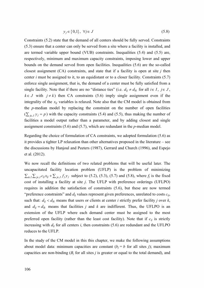
106

0,1jy , j J (5.8)

Constraints (5.2) state that the demand of all centers should be fully served. Constraints

(5.3) ensure that a center can only be served from a site where a facility is installed, and

are termed variable upper bound (VUB) constraints. Inequalities (5.4) and (5.5) are,

respectively, minimum and maximum capacity constraints, imposing lower and upper

bounds on the demand served from open facilities. Inequalities (5.6) are the so-called

closest assignment (CA) constraints, and state that if a facility is open at site j then

center i must be assigned to it, to an equidistant or to a closer facility. Constraints (5.7)

enforce single assignment, that is, the demand of a center must be fully satisfied from a

single facility. Note that if there are no “distance ties” (i.e. ij ikd d for all i I , j J ,

k J with j k ) then CA constraints (5.6) imply single assignment even if the

integrality of the ijx variables is relaxed. Note also that the CM model is obtained from

the p-median model by replacing the constraint on the number of open facilities

( jj J y p ) with the capacity constraints (5.4) and (5.5), thus making the number of

facilities a model output rather than a parameter, and by adding closest and single

assignment constraints (5.6) and (5.7), which are redundant in the p-median model.

Regarding the choice of formulation of CA constraints, we adopted formulation (5.6) as

it provides a tighter LP relaxation than other alternatives proposed in the literature – see

the discussions by Hanjoul and Peeters (1987), Gerrard and Church (1996), and Espejo

et al. (2012).

We now recall the definitions of two related problems that will be useful later. The

uncapacitated facility location problem (UFLP) is the problem of minimizing

ij ij j ji I j J j Jc x f y subject to (5.2), (5.3), (5.7) and (5.8), where fj is the fixed

cost of installing a facility at site j. The UFLP with preference orderings (UFLPO)

requires in addition the satisfaction of constraints (5.6), but these are now termed

“preference constraints” and dij values represent given preferences, unrelated to costs cij,

such that: ij ikd d means that users or clients at center i strictly prefer facility j over k,

and ij ikd d means that facilities j and k are indifferent. Thus, the UFLPO is an

extension of the UFLP where each demand center must be assigned to the most

preferred open facility (rather than the least cost facility). Note that if cij is strictly

increasing with dij for all centers i, then constraints (5.6) are redundant and the UFLPO

reduces to the UFLP.

In the study of the CM model in this this chapter, we make the following assumptions

about model data: minimum capacities are constant (bj = b for all sites j); maximum

capacities are non-binding (Bj for all sites j is greater or equal to the total demand), and

107

thus constraints (5.5) can be dropped from the formulation. Let X LSC denote the feasible

set of the CM model with those assumptions, i.e. the set of the location model with

constant lower capacity bounds (L), single assignment (S) and closest assignment (C):

X LSC = {0,1} , {0,1} :n m mx y (5.2), (5.3), (5.4), (5.6) are satisfied,

assuming jb b for j J

We will study valid inequalities for the following sets:

X UFLPO = {0,1} , {0,1} :n m mx y (5.2), (5.3), (5.6) are satisfied

X LS = {0,1} , {0,1} :n m mx y (5.2), (5.3), (5.4) are satisfied,

assuming jb b for j J

X LSI = {0,1} , {0,1} :n m mx y (5.2), (5.3), (5.4), ii ix y for i I are satisfied,

assuming I J , and ib b for i I

Sets X UFLPO and X LS are relaxations of (i.e. contain) the set X LSC. Set X LSI is a relaxation

of a variant of X LSC restricted to: (1) identical sets of centers and sites (I = J); (2)

ii ix y for i I , i.e. facilities must serve the centers where they are located. Note that

when I = J and dij data is such that dii is the unique, minimum distance for i I , then the

CA constraints (5.6) for i I and j i reduce to ii ix y , and combined with (5.3) give

ii ix y .

Before continuing, we note that the CM model is NP-hard, since the UFLP, which is

NP-hard (Cornuejols et al., 1990), can be polynomially reduced to it. An instance of the

UFLP can be transformed into an instance of the CM model by the following procedure,

using closest assignment constraints to include fixed costs in the objective function

through equivalent variable costs. (1) For i I, j J, set cij as in the original UFLP

data and set dij = 0. (2) Create a set I’ of fictitious centers corresponding to sites in J; for

i I’, j J, set cij = fj if i = j or equal to zero otherwise, and set dij = 0 if i = j or equal

to any positive value otherwise. (3) Augment the set I with set I’ and set all other data

(ui, bj, Bj) to zero. A similar procedure was cited by Hansen et al. (2004) to reduce the

UFLPO to a restricted UFLPO without fixed costs ( fj = 0 for all sites j), thus showing

that even this restricted problem is NP-hard.

5.3 Valid inequalities for X UFLPO

We first introduce additional notation related to the preference (or closest assignment)

constraints. For i I , j J :

108

|ij ik ijW k J d d (worse/farther sites)

\ |ij ij ik ijN J W k J d d (not worse/farther sites)

|ij ik ijE k J d d (indifferent/equidistant sites)

\ |ij ij ij ik ijN N E k J d d (strictly better/closer sites)

In his PhD thesis, García (2006) studied several valid inequalities for X UFLPO and

proposed the reformulation procedure cited above, later also published by Cánovas et al.

(2007). These authors assumed data with no preference ties, i.e. Eij = {j} holds for all i

and j. Next we review relevant inequalities and discuss the case of data with preference

ties, i.e. |Eij| 1.

Dominance inequalities – assuming no preference ties, |Eij| = 1 (Cánovas et al., 2007):

1 2i j i jx x , for 1 2, ,i i I j J : 1 2i j i jW W (or 1 2i j i jN N )

1 2i j i jx x , for 1 2, ,i i I j J : 1 2i j i jW W (or 1 2i j i jN N )

The first inequality states that assigning i1 to j implies also assigning i2 to j if all sites

better than j for i1 are also better than j for i2. The equality results from combining two

inequalities.

Inequality 1 2i j i jx x dominates the VUB constraint 1i j jx y , since 2i j jx y is also in

the model, and can be used to strengthen the formulation. Thus, as noted by Cánovas et

al. (2007), while all VUB constraints are facet defining for the UFLP polytope

(Cornuejols et al., 1990), this is not the case for the UFLPO polytope, depending on dij

data. Next we present a generalization for data with preference ties.

Dominance inequalities – generalized for preference ties, |Eij| 1:

1 2i j i jx x , for 1 2, ,i i I j J : 1 2 \i j i jN N j (A)

1 2i j i jx x , for 1 2, ,i i I j J : 1 2i j i jN N and 1 2i j i jE E j (Aeq)

Proof of validity of (A): If 1 0i jx the inequality is trivially valid. If 1 1i jx then it must

be 1jy and 0ky for 1i jk N in order to satisfy (5.3) and (5.6), respectively. Then,

(5.3) implies 2 0i kx for 1i jk N , and, given that 1 2 \i j i jN N j , (5.6) implies

2 1i jx .

Proof of validity of (Aeq): As ij ij ijN N E , inequalities (A) hold for both 1 2( , )i i and

2 1( , )i i if 1 2 2 \{ }i j i j i jN N E j and 2 1 1 \{ }i j i j i jN N E j , which leads to the

conditions given.

109

Preference inequalities (Cánovas et al., 2007):

1

1

1i j

i k jk W

x y

, for 1 ,i I j J (C1)

1 2

1 2 1\

1i j i j i j

i k i k jk W k W W

x x y

, for 1 2, ,i i I j J (C2)

11

11

2 \

1tt

i j i j i jt rr

s

i k i k jk W t k W W

x x y

, for 1,..., ,si i I j J (Cs)

Inequalities (C1) are equivalent to (5.6), as demand constraints (5.2) imply that

1ij ijik ikk N k Wx x for all i I , j J . The two formulations can be interpreted as

follows: if facility j is open, (C1) forbids assignment to worse facilities, while (5.6)

forces assignment to better or indifferent facilities. Note that formulation (5.6) implies

that all centers must be assigned if at least one facility is open, while (C1) is compatible

with models where not all demand requires satisfaction, i.e. with “=” replaced by “” in

(5.2).

Inequalities (C2) and (Cs) are generalizations of (C1). Although inequalities (C1) can be

dominated by the others, e.g. by (C2) for 1 2, ,i i I j J such that 2 1\i j i jW W ,

Cánovas et al. (2007) chose not to replace all such dominated inequalities (C1), since,

according to their experiments, the improvement of LP bounds would not compensate

the increase of the number of non-zero elements. However, a particular case is exploited

in the reformulation: if 1 2i j i jW W , inequality (C2) for 1 2( , , )i i j dominates the two

(C1) inequalities for 1( , )i j and 2( , )i j while not increasing formulation size (this applies

similarly to the generalized (Cs) inequalities). Finally, we note that the inequalities

above remain valid when data has preference ties.

W inequalities (García, 2006):

1 2

1 1i j i j

i k i kk W k W

x x

, for 1 2, ,i i I j J . (W)

1 2i k i kk S k S

x x

, for 1 2, , ,i i I j h J : 1 2i j i hS W W . (Weq)

Proof of validity of (W): If the left-hand side is zero, the inequality is trivially valid. If

111

i j i kk W x then, for 1\ i jk J W , (5.2) implies 1 0i kx , (5.6) requires 0ky , and

(5.3) implies 2 0i kx for all 2i I . Thus, for all 2i I , 21\ 0i j i kk J W x and (5.2)

requires 211

i j i kk W x .

Proof of validity of (Weq): The equality follows from combining (W) for 1 2( , , )i i j and

for 2 1( , , )i i h .

110

Inequality (W) states that assigning i1 to facilities it prefers less than j implies also

assigning all other centers to those facilities (since all others must be closed). Equality

(Weq) states that if sites in set S are the worst for both i1 and i2 (but possibly ordered

differently), then i1 and i2 must be either both assigned to facilities in S or both not

assigned to facilities in S. The proof of (W) above uses the same arguments as the one

by García (2006). We also note that (W) and (Weq) remain valid when data has

preference ties.

Inequality (W) for 1 2( , , )i i j dominates inequality (C1) 111

i j i k jk W x y if 1 2i j i jW W ,

since 1 21 1i j i ji k i kk W k Wx x 22i j i kk W x 1 jy , following respectively from (W),

1 2i j i jW W , and (C1) for 2( , )i j . However, Cánovas et al. (2007) do not exploit this in

the reformulation since replacing all such dominated (C1) inequalities would again not

be compensated by the increase of the number of non-zero elements.

Inequalities (W) (actually, slightly less general variants) were independently introduced

by Belotti et al. (2007) and Vasilyev et al. (2009), and were exploited to generate cuts in

branch-and-cut algorithms by Belotti et al. (2007) and Vasilyev and Klimentova (2010).

In this chapter, we exploit (Weq) in an additional step of the reformulation procedure

and exploit (W) to generate cuts in a branch-and-cut algorithm. Finally, we note that

García (2006) presented additional new valid inequalities for X UFLPO which are not

useful for the a priori reformulation but may be useful to generate cuts. However, they

were not tested by García (2006), nor in later work by any author, as far as we know.

5.4 Reformulation procedure for X UFLPO

We next present an a priori reformulation procedure for the UFLPO that aims to

strengthen the formulation and reduce its size (in terms of number of variables,

constraints and non-zero elements) before applying a branch-and-cut algorithm. The

procedure depends on the particular data of each instance, specifically on the dij data

underlying CA constraints (5.6), and makes use of inequalities (Aeq), (A), (Weq), and

(Cs). This procedure is based on work by Cánovas et al. (2007), and is here extended for

data with dij ties and with an additional step.

Step 1 (use (Aeq) to strengthen VUB constraints). For j J and 1 2, ,..., si i i I ,

1 ... si i , such that 1 ... si j i jN N and 1 ... si j i jE E j : replace constraint ij jx y

with 1ij i jx x for 2 ,..., si i i . The variables 2 ,..., si j i jx x are termed replaced in the next

step.

111

Step 2 (use (A) to strengthen VUB constraints). For j J and 1 2,i i I , 1 2i i , such

that 1 2 \i j i jN N j : replace constraint 1i j jx y with 1 2i j i jx x if (i) both variables 1i jx

and 2i jx were not replaced in step 1, and (ii) 1 2i j i jx x is not dominated, i.e. no 3i I ,

3 1 2,i i i , exists such that 1 3i j i jx x and 3 2i j i jx x also hold. In addition, if more than

one such 2i I exists, only one inequality is added so as not to enlarge the model. In

this case, the minimum lexicographic index is chosen.

Step 3. New step, described further below.

Step 4 (remove trivially redundant CA constraints). For i I : (1) if a unique j J

exists such that 1ijN , remove the CA constraint for (i, j), which reduces to ij jx y ,

and replace VUB constraint ij jx y with ij jx y ; (2) for j J such that ijN m ,

remove the CA constraint for (i, j), which reduces to 1 jy .

Step 5 (use (Cs) to strengthen CA constraints). For j J , let T I such that 2T ,

ijW for all i T and 1 2i j i jW W for all 1 2,i i T . Replace CA constraints

ij ik jk N x y for i T with 1ij ik ji T k W x y .

Cánovas et al. (2007) describe the following algorithm to find sets T. For each j J :

(1) define : :ij tj ij tjS i I W t I W W W and construct a graph

( , )S A with set of arcs 1 21 2( , ) : i j i jA i i S S W W ; (2) search a clique T in the

graph and replace CA constraints for i T as described above; (3) remove the nodes in

T from the graph and return to the previous step until no edges remain in the graph.

García (2006) includes the following further remarks. This procedure does not search

for all possible cliques, in order to avoid increasing model size. In step (2), the clique is

selected by adding elements remaining in S in lexicographic order (although alternative

heuristic rules would be possible).

Step 6 (reduce the number of non-zero elements in CA constraints). For each CA

constraint (original or strengthened in the previous step), if ij ijW N replace

ij ikk N x by 1ij ikW x . This changes formulation (5.6) into (C1).

Notes:

All steps above were part of the original procedure of Cánovas et al. (2007). The

conditions of steps 1, 2 and 4 were modified to account for ties in dij data. The

original steps 5 and 6 were valid with such ties, and remain unaltered in this

respect. In steps 2 and 5, the original rules were retained to select among

multiple alternative inequalities, when they exist. However, step 5 considers

112

only the CA constraints which are not dropped in step 3, which is described

below.

The presolve routine of a MIP optimizer will automatically perform step 4, so

this step could be dropped. It will also eliminate redundant variables after steps

1 and 4 even if they are kept in the initial formulation, which is useful to

simplify the implementation.

Church (2003) proposed a reformulation of the p-median model, called COBRA,

including a step equivalent to step 1 above.

We next introduce an additional reformulation step exploiting equalities (Weq). The

following additional notation is used:

CA(i, j) denotes CA constraints (5.6) for a particular pair of centers and sites

(i, j), and 1 2( , , )eqW i i j is similar notation for (Weq);

1 2( , , )EQ i i A := 1 2i k i kk A k Ax x for 1 2,i i I , A J .

We start with some preliminary remarks. For 1 2,i i I and 1 2,j j J :

Remark 1: If 1 1 2 2i j i jA N N , then 1 2 1( , , )eqW i i j = 1 2 2( , , )eqW i i j = 1 2( , , \ )EQ i i J A and,

given demand constraints (5.2), this equality is equivalent to 1 2( , , )EQ i i A .

Remark 2: If 1 1 2 2i j i jA N N and 1 1 2 2i h i hB N N with 1 2,h h J and A B , then we

can write the three equalities 1 2( , , )EQ i i A , 1 2( , , \ )EQ i i B A , and 1 2( , , )EQ i i B . Only two

are independent and the first two have the least number of non-zero elements.

Remark 3: If 1 1 2 2i j i jA N N and equality 1 2( , , )EQ i i A is added to the formulation,

then one or more CA constraints become redundant or dominated. In the following, we

recall that 1 2( , , )EQ i i A := 1 2i k i kk A k Ax x and ( , )CA i h :=ih ik hk N x y .

i) For 1 1 2 2i j i jh E E , and thus 1 2i h i hN N A , 1( , )CA i h and 2( , )CA i h are

equivalent and one can be dropped, e.g. the latter.

ii) For 1 1 2 2\i j i jh E E , and thus 2 1i h i hN N A , 1( , )CA i h is dominated by

2( , )CA i h and can be dropped.

iii) For 2 2 1 1\i j i jh E E , and thus 1 2i h i hN N A , 2( , )CA i h is dominated by

1( , )CA i h and can be dropped.

If no dij ties exist, i.e. 1 1 1i jE j and 2 2 2i jE j , there are two cases: if

1 2j j , part (i) applies and either 1 1( , )CA i j or 2 2( , )CA i j can be dropped; if

113

1 2j j , parts (ii) and (iii) apply and both 1 1( , )CA i j and 2 2( , )CA i j can be

dropped.

Regarding the number of non-zero elements when 1 2( , , )EQ i i A is added and

redundant CA constraints are dropped: it increases if 1 1 2 2 1i j i jE E and

1 2j j and 1A ; otherwise, it does not increase or decreases.

The new step uses the remarks above and is as follows.

Step 3 (add equalities (Weq) and remove redundant CA constraints)

Step 3.1 (add EQ). For 1 2,i i I | 2 1i i , find ,h hj j J for 1,...,h s such that hS

1 2h hi j i jN N and 0 1 ... sS S S J . For 1,...,h s , set 1\h h hT S S and add

1 2( , , )hEQ i i T to the formulation if it is not redundant, i.e. if all of the following are

false:

1. hT J . In this case, the only equality that can be written for the pair (i1, i2) is

dominated by demand constraints (5.2).

2. 1hT . In this case, the equality was already added in step 1.

3. Equalities 1i j ijx x for some i I and all hj T were added in step 1, and

2( , , )hEQ i i T was already added in step 3.

4. Equalities 2i j ijx x for some i I and all hj T were added in step 1, and

1( , , )hEQ i i T was already added in step 3.

5. Equality 1( , , )hEQ i i T was already added for some i I : 1i i . In this case,

2( , , )hEQ i i T was also already added or is implied by other added equalities.

6. h mT T : arg max 1,..., : km k s T . Since one equality will be redundant,

given demand constraints (5.2), choose one with the maximum number of

elements (if more than one exists, pick the lexicographic minimum m).

Step 3.2 (drop CA). For 1 2,i i I , 1 2,j j J | 1 1 2 2i j i jA N N : drop CA constraints

according to Remark 3 above. In all cases, 1 2( , , )EQ i i A is valid and is implied by the

formulation after step 3.1. Includes the special case 1 1 2 2 1i j i jE E and 1 2j j ,

corresponding to the equalities added in step 1.

The computational performance of the reformulated model is presented in the results

section, including a comparison between the UFLPO and the CM model.

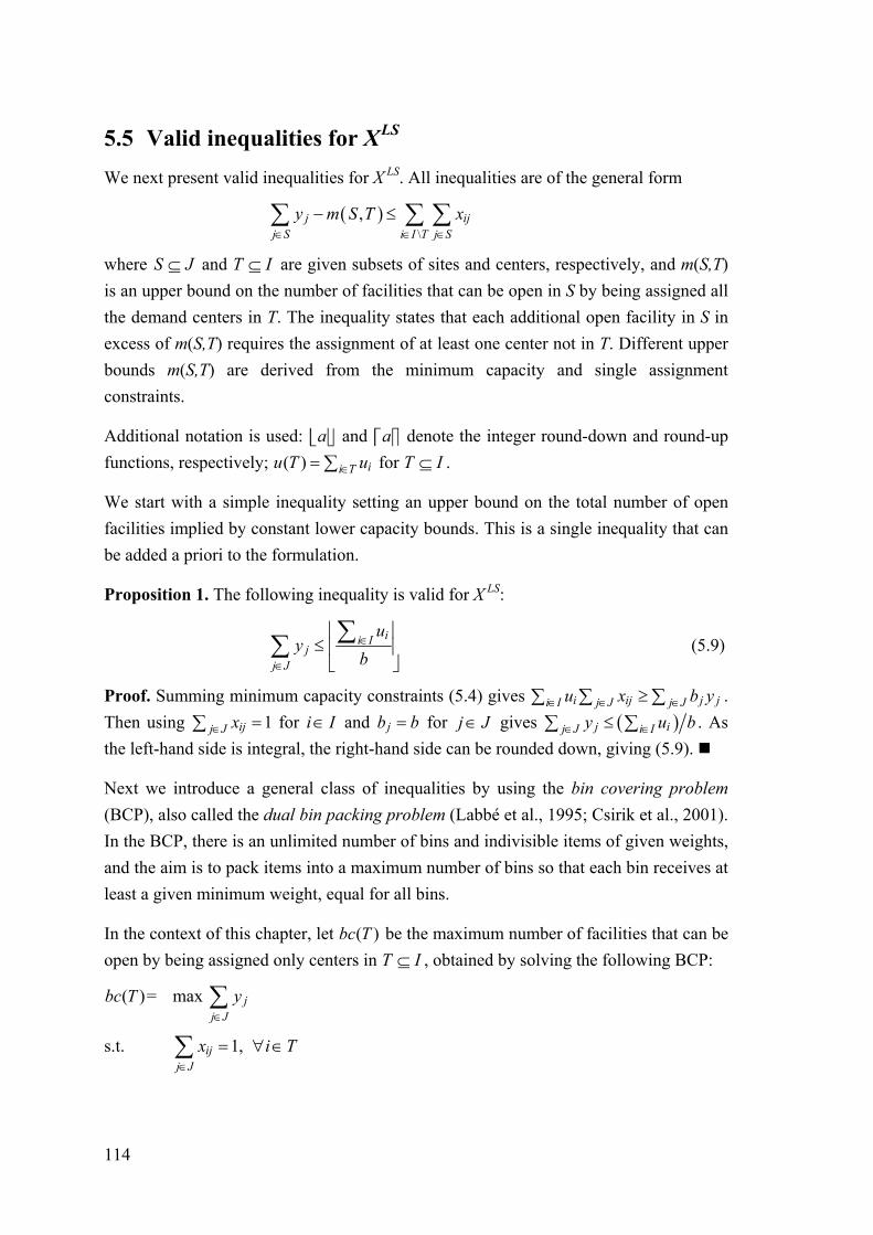
114

5.5 Valid inequalities for X LS

We next present valid inequalities for X LS. All inequalities are of the general form

\

,j ijj S i I T j S

y m S T x

where S J and T I are given subsets of sites and centers, respectively, and m(S,T)

is an upper bound on the number of facilities that can be open in S by being assigned all

the demand centers in T. The inequality states that each additional open facility in S in

excess of m(S,T) requires the assignment of at least one center not in T. Different upper

bounds m(S,T) are derived from the minimum capacity and single assignment

constraints.

Additional notation is used: a and a denote the integer round-down and round-up

functions, respectively; ( ) ii Tu T u for T I .

We start with a simple inequality setting an upper bound on the total number of open

facilities implied by constant lower capacity bounds. This is a single inequality that can

be added a priori to the formulation.

Proposition 1. The following inequality is valid for X LS:

ii I

jj J

uy

b

(5.9)

Proof. Summing minimum capacity constraints (5.4) gives i ij j ji I j J j Ju x b y .

Then using 1ijj J x for i I and jb b for j J gives j ij J i Iy u b . As

the left-hand side is integral, the right-hand side can be rounded down, giving (5.9).

Next we introduce a general class of inequalities by using the bin covering problem

(BCP), also called the dual bin packing problem (Labbé et al., 1995; Csirik et al., 2001).

In the BCP, there is an unlimited number of bins and indivisible items of given weights,

and the aim is to pack items into a maximum number of bins so that each bin receives at

least a given minimum weight, equal for all bins.

In the context of this chapter, let ( )bc T be the maximum number of facilities that can be

open by being assigned only centers in T I , obtained by solving the following BCP:

( )bc T = max jj J

y

s.t. 1ijj J

x

, i T

115

i ij ji T

u x by

, j J

0,1ijx , 0,1jy , ,i T j J

Proposition 2. Let S J , T I and ( )bc T be the optimal value of the bin covering

problem with demand set T and minimum capacity b. The following bin covering

inequality is valid for X LS:

\

( )j ijj S i I T j S

y bc T x

(5.10)

Proof. Suppose that ( )jj S y bc T k . If 0k , the inequality is trivially valid. So

suppose that 1k . By definition, at most ( )bc T open facilities can satisfy the minimum

capacity constraints (5.4) with only the demand from T. Thus, at least k open facilities

in S require additional demand from I \ T to satisfy (5.4). Because of single assignment

constraints (5.7), this implies \ iji I T j S x k , and thus the inequality is valid.

We observe that bin covering inequalities are the analogue for constant minimum

capacities of the bin packing inequalities studied by Deng and Simchi-Levi (1992) and

by Labbé and Yaman (2006) for the polytope of the capacitated facility location

problem (CFLP) with single assignment and constant maximum capacities.

Since there are an exponential number of inequalities (5.10), particular cases that can be

added to the formulation a priori or as cuts may be useful in practice. To use (5.10) it is

necessary to choose sets S and T and to compute ( )bc T . We observe that ( )S bc T

must hold for the inequality not to be redundant, and T should be maximal for the

inequality to be tight, i.e. T T such that ( ) ( )bc T bc T produces a dominated

inequality.

If ( )bc T is replaced in (5.10) by an upper bound ( )U bc T , a weaker but still valid

inequality is obtained. This is useful to avoid computing ( )bc T since the BCP is NP-

hard, as noted by Labbé et al. (1995). The same authors present reduction criteria, upper

bounds, lower bounds and a branch-and-bound algorithm for the BCP. They assume

first that iu b , i T . The four upper bounds provided are: 0 2U T ;

1 ( )U u T b ; and two other bounds 2U and 3U that can be computed in ( )O n time

assuming items are sorted by weight. 2U dominates the two first bounds, i.e.

2 0 1min ,U U U , and the best bound is 2 3min ,U U U .

Note that by using S = J and T = I in (5.10) we get the following inequality dominating

(5.9), whose right-hand side is the upper bound U1:

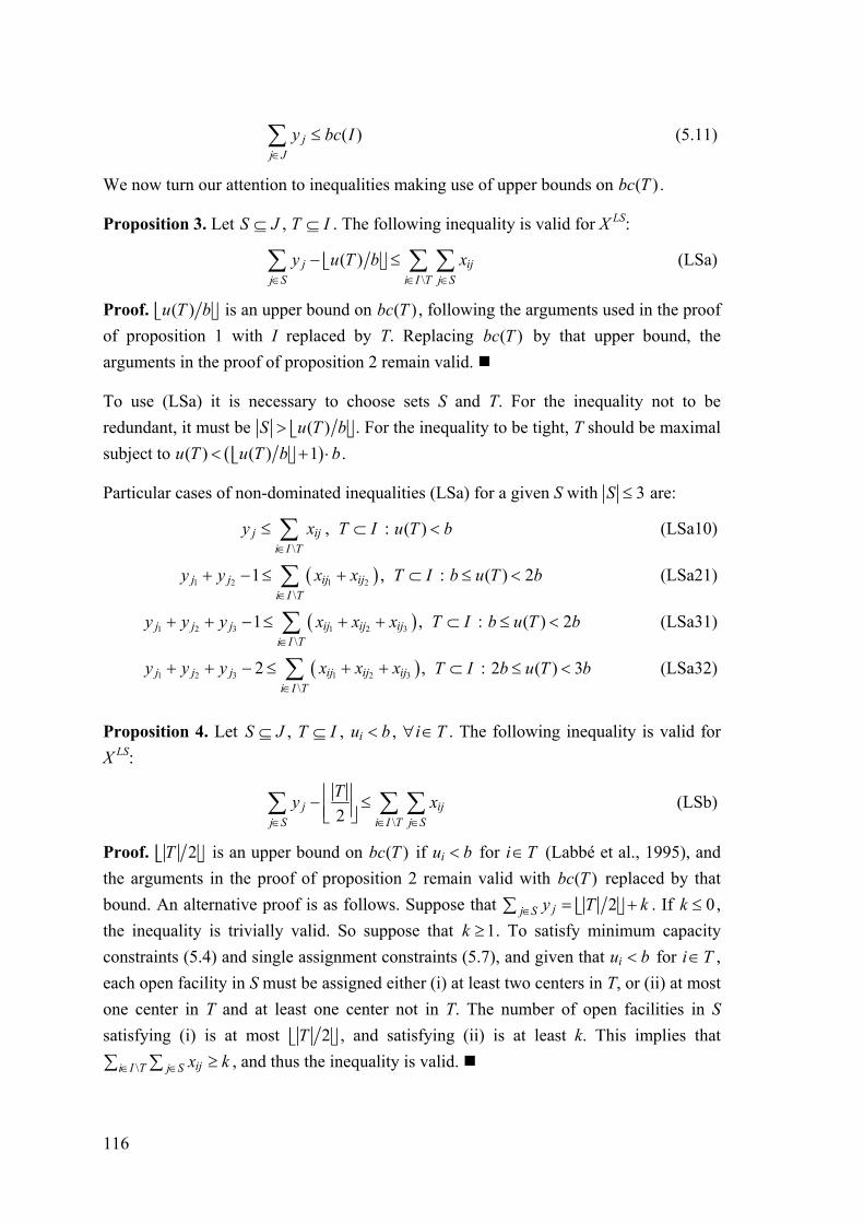
116

( )jj J

y bc I

(5.11)

We now turn our attention to inequalities making use of upper bounds on ( )bc T .

Proposition 3. Let S J , T I . The following inequality is valid for X LS:

\

( )j ijj S i I T j S

y u T b x

(LSa)

Proof. ( )u T b is an upper bound on ( )bc T , following the arguments used in the proof

of proposition 1 with I replaced by T. Replacing ( )bc T by that upper bound, the

arguments in the proof of proposition 2 remain valid.

To use (LSa) it is necessary to choose sets S and T. For the inequality not to be

redundant, it must be ( )S u T b . For the inequality to be tight, T should be maximal

subject to ( ) ( ) 1u T u T b b .

Particular cases of non-dominated inequalities (LSa) for a given S with 3S are:

\

j iji I T

y x

, T I : ( )u T b (LSa10)

1 2 1 2

\

1j j ij iji I T

y y x x

, T I : ( ) 2b u T b (LSa21)

1 2 3 1 2 3

\

1j j j ij ij iji I T

y y y x x x

, T I : ( ) 2b u T b (LSa31)

1 2 3 1 2 3

\

2j j j ij ij iji I T

y y y x x x

, T I : 2 ( ) 3b u T b (LSa32)

Proposition 4. Let S J , T I , iu b , i T . The following inequality is valid for

X LS:

\2

j ijj S i I T j S

Ty x

(LSb)

Proof. 2T is an upper bound on ( )bc T if iu b for i T (Labbé et al., 1995), and

the arguments in the proof of proposition 2 remain valid with ( )bc T replaced by that

bound. An alternative proof is as follows. Suppose that 2jj S y T k . If 0k ,

the inequality is trivially valid. So suppose that 1k . To satisfy minimum capacity

constraints (5.4) and single assignment constraints (5.7), and given that iu b for i T ,

each open facility in S must be assigned either (i) at least two centers in T, or (ii) at most

one center in T and at least one center not in T. The number of open facilities in S

satisfying (i) is at most 2T , and satisfying (ii) is at least k. This implies that

\ iji I T j S x k , and thus the inequality is valid.

117

To use (LSb) it is necessary to choose sets S and T. For the inequality not to be

redundant, it must be 2T S . For the inequality to be tight, |T| should be odd (given S

and T with |T| even, adding an element to T produces a tighter inequality). Comparing

(LSb) and (LSa), if 2S then (LSb) is dominated by (LSa), specifically by (LSa10) or

(LSa21). If 3S , no inequality always dominates the other.

Particular cases of inequalities (LSb) for a given S with 3S and for 3T are:

1 2 3 1 2 3

\

1j j j ij ij iji I T

y y y x x x

, T I : 3T , iu b , i T (LSb31)

Inequality (LSb31) is only useful if ( ) 2u T b , otherwise it is dominated by (LSa31) or

by a combination of (LSa10) for all elements of S.

5.6 Valid inequalities for X LSI

We now consider set X LSI, i.e. the restriction of X LS assuming I = J and xii = yi for i I .

These conditions allow some of the previous inequalities to be strengthened.

Proposition 5. Let S T I , iu b , i S . The following inequality is valid for X LSI:

\

2 j ijj S i I T j S

y T x

(LSc)

or, equivalently,

\

22

j ijj S i I T j S

Ty x

, if T is even

\

2 12

j ijj S i I T j S

Ty x

, if T is odd

Proof. Suppose that 2jj S y T k . If 0k , the inequality is trivially valid. So

suppose that 1k . Thus there are 2A T k centers in S with open facilities,

assigned to their own facilities, as ii ix y for i I . Since by assumption iu b for

i S , in order to satisfy minimum capacity constraints (5.4) and single assignment

constraints (5.7), each open facility in S must additionally be assigned either (i) at least

one other center in T or (ii) at least one center in I \ T. The number of open facilities in S

satisfying (i) is at most B T A , and satisfying (ii) is at least

2 2 2 2A B A T T k T . This implies that \ 2iji I T j S x k if T is

even, or \ 2 1iji I T j S x k if T is odd, and thus the inequality is valid.

To use (LSc) it is necessary to choose sets S and T and it must be 2T S for the

inequality not to be redundant. Comparing (LSc) and (LSb) for given S and T, if T is

118

even then (LSc) dominates (LSb). If T is odd, the left-hand side of (LSc) is higher than

the one of (LSb) when 2 1jj S y T ; thus, (LSc) is dominated by (LSb) if

2 1S T (e.g. 2, 3S T ) and iu b for i T (this condition is required by

(LSc) only for i S ); otherwise, no inequality always dominates the other.

Particular cases of inequalities (LSc) for a given S with S 2 or 3 and T = S are:

1 2 1 2

\

2 1j j ij iji I T

y y x x

, T S I : iu b , i S (LSc21)

1 2 3 1 2 3

\

2 1 1j j j ij ij iji I T

y y y x x x

, T S I : iu b , i S (LSc31)

5.7 Separation procedures

In this section we present separation procedures for some of the valid inequalities from

the previous sections in order to exploit them in a branch-and-cut algorithm. The

separation problem associated with a given family of inequalities F for a formulation P

is defined as follows. Given a fractional solution ( , ) n m mx y R R obtained by

solving the LP relaxation of P, find an inequality of family F that is violated by ( , )x y

or show that no such inequality exists.

For X LS and X LSI, we restricted our attention to inequalities with sets of small cardinality

3S , corresponding to particular cases presented before. It is also assumed that I J

and that demand and capacity data is integer.

Separation of inequalities (LSa10). For each j J such that ju b and 0jy , find

the set T that maximizes iji T x subject to ( ) 1u T b , which is a binary knapsack

problem. If \j iji I T j Sy x , the inequality is violated and is added to the

formulation. Separation run time is O(n2 log n) if the knapsack problem is solved

approximately by the standard greedy heuristic (Martello and Toth, 1990), requiring

O(n log n) time.

Separation of inequalities (LSa21). For each S J such that 2S , ( ) 2u S b and

1jj S y , find the set T that maximizes iji T j S x subject to ( ) 2 1u T b , which

is a binary knapsack problem. If \1j ijj S i I T j Sy x , the inequality is violated

and is added to the formulation. Separation run time is O(n3 log n) using the greedy

knapsack heuristic.

Separation of inequalities (LSa31). For each S J such that 3S , ( ) 2u S b and

1jj S y , find the set T as for inequalities (LSa21). If the inequality is violated, add it

119

to the formulation. Separation run time is O(n4 log n) using the greedy knapsack

heuristic.

Separation of inequalities (LSb31) and (LSc31). For each S J such that 3S ,

iu b for i S , and 1jj S y , check if inequality (LSb31) is violated for T S . If so,

add it to the formulation. If 2jj S y , then inequality (LSc31) is violated by a larger

amount and is added instead. Separation run time is O(n3).

Separation of inequalities (W). The procedure of Belotti et al. (2007) was used. For

each 1i I , find 2i I and j J that most violate inequality (W), and add all found

violated inequalities to the formulation. Running time is O(n3) and up to n inequalities

are added per iteration.

In the computational experiments performed, the greedy knapsack heuristic was

replaced by the exact procedure MT1 of Martello and Toth (1990), since this was still

very fast for the instance sizes tested.

5.8 Computational experiments

Computational experiments were carried out with the CM model. The objective was to

compare three solution methods using a generic MIP optimizer implementing a branch-

and-cut algorithm:

S – standard formulation;

R – a priori reformulation;

RC – a priori reformulation and special purpose cuts (or user cuts) in addition to

automatic cuts.

The software used was FICO’s Xpress Optimization Suite version 2005B (released in

Nov. 2005). The model formulation and code for the reformulation and separation (cut

generation) procedures were implemented with Xpress Mosel 1.6, and the model was

solved with Xpress MIP Optimizer 16.10. The computer used had a Pentium M 755 2.0

GHz CPU, 1.0 GB of memory, and Windows XP operating system.

Formulation (5.1)-(5.8) was used with the following assumptions: identical sets of

centers and sites (I = J); constant minimum capacities (bj = b for all sites j); non-binding

maximum capacities (Bj is greater or equal to total demand for all sites j), and thus

constraints (5.5) were dropped from the formulation. Constraint (5.9) was added a priori

to the formulation. The simple upper bound in (5.9) could have been replaced by the

tightest bin covering upper bound of Labbé et al. (2005) mentioned in section 5.5, but

120

this would make no difference in our tests since the two bounds were equal in the

instances tested.

Regarding user cuts, after preliminary experiments the following procedure was

adopted. Cuts are generated from inequalities (W) and (LSa10) only, as the others

referred to in the previous section led to increased solution times in preliminary

experiments. Cuts are generated at the top node only (after automatic cut generation).

Only cuts violated more than a given threshold are added (0.01 was used). In each

round, cuts of a single type are added. All added cuts remain in the formulation,

including those that become inactive in later rounds.

Regarding solver parameters, branching priority was given to y variables (in preliminary

tests this reduced solution time significantly, by 5-60%). A time limit of 1 hour was

imposed. All other parameters were left at default values, except for method RC where

presolve was disabled (to avoid interference of variable elimination with user cut

generation).

Test instances were randomly generated as follows. First, for a given size n (number of

centers), 9 data sets (cij, ui) were created: points representing centers were uniformly

generated in [0,100][0,100]; ui = 1000/nUniform[0.1,1.9]; cij = uidij, where dij is the

Euclidean distance between centers i and j. Then, the capacity ratio r, equal to total

demand divided by the minimum capacity (i.e. the expected maximum number of open

facilities), was used as a control parameter to derive 4 instances from each data set

(cij, ui) by setting ii Ib u r for r = n0.1, 0.2, 0.3, and 0.4. All data was rounded to

integer values.

Results are reported in the tables below, with the following definitions:

n-r: instance group, defined by size n and capacity ratio r;

inst.: number of the individual instance;

IP: optimal value;

nf: number of facilities in an optimal integer solution;

finished: 1 if the instance was solved to optimality within the time limit, 0

otherwise;

time: total solution time in seconds; includes the time for the reformulation

procedure and user cut generation, if applicable (note: the reported time of

unfinished instances may exceed the imposed limit of 3600, since this excludes

time for the a priori reformulation procedure and the first LP relaxation);

nodes: number of nodes in the branch-and-bound tree;

121

gaps: gapLP=(IP-LP)/IP, gapXLP=(IP-XLP)/IP, gap closed=(XLP-LP)/(IP-LP),

where LP is the value of the first LP relaxation, XLP is the value of the LP

relaxation at the top node after addition of cuts, and IP is the optimal value;

acuts and ucuts: number of cuts added at the top node by the automatic and user

procedures, respectively; the number of generated automatic cuts may be higher,

as cuts that become inactive in successive cut generation iterations are deleted;

Table 5.1 and Table 5.2 summarize results of individual instances in Table 5.3, where:

“avg” denotes arithmetic averages of results of individual instances;

gap closed with methods S, R and RC is relative to the LP value with method S;

time ratio A/B is the time with method A divided by the time with method B,

computed for individual instances.

First we observe that instances with smaller capacity ratios (r/n=0.1 and 0.2) are harder

to solve than those with larger ratios (r/n=0.3 and 0.4). Method R relatively to S solves

more instances within the time limit and reduces time by about 60% on average and by

20-90% for different instance groups (Table 5.1). LP and XLP gaps are also reduced

(Table 5.2) and the number of nodes decreases significantly (Table 5.1), considering

instance groups with comparable number of finished instances. Method RC relatively to

R helps at further reducing XLP gaps and the number of nodes (but LP gaps with RC

are larger, because presolve is disabled). Solution time decreases by about 30%

relatively to method R for instances with r/n=0.2 (70-14 and 100-20), but for other

instances time increases or is only slightly reduced. Thus we conclude that the

reformulation procedure is very effective, while the user cuts are not generally effective.

The explanation for the poor performance of user cuts is mainly that these cuts are

relatively weak, i.e. the additional LP gap closed relatively to automatic cuts is small.

For most instance groups, this gap reduction is not compensated by the increase in

number of rows and non-zero elements. It was verified that positive time differences

between methods RC and R are not explained by presolve being disabled in RC (if it is

also disabled in R, differences are still positive), nor by user cut generation time being

excessive (it is lower than those differences). Also, if inactive cuts are deleted in user

cut generation routines (instead of being managed automatically by the solver), the

solution time is similar.

122

Table 5.1: Summary of results – nodes and time

n-r total finished avg nodes avg time avg time ratios

S R RC S R RC S R RC R/S RC/S RC/R

70-7 9 9 9 2035 1529 1195 661 262 409 0.45 0.74 1.64

70-14 8 9 9 9423 3106 1080 1771 383 228 0.27 0.18 0.70

70-21 9 9 9 1430 279 170 241 47 51 0.29 0.32 1.14

70-28 9 9 9 309 13 8 64 17 22 0.41 0.51 1.26

70 total 35 36 36 3300 1232 613 685 178 178 0.36 0.44 1.18

100-10 1 3 2 1430 3728 1776 3495 2956 2951 0.83 0.83 0.96

100-20 1 6 8 2236 6022 1969 3344 2261 1323 0.64 0.38 0.67

100-30 4 9 9 3618 949 184 2819 292 192 0.11 0.09 0.90

100-40 8 9 9 4275 101 63 1723 80 95 0.10 0.12 1.22

100 total 14 27 28 2889 2700 998 2845 1397 1140 0.42 0.35 0.94

Table 5.2: Summary of results – gaps

n-r avg gapLP (%) avg gapXLP (%) avg gap closed (%)

S R RC S R RC S R RC

70-7 5.6 5.6 5.6 4.8 4.5 3.6 19 25 39

70-14 9.9 9.7 9.7 6.4 4.9 3.3 36 52 68

70-21 13.7 12.7 13.5 4.4 2.5 1.7 70 83 88

70-28 15.5 13.5 20.6 3.1 1.0 0.8 80 94 95

70 total 11.2 10.3 12.3 4.7 3.2 2.4 51 64 73

100-10 6.9 6.7 6.7 6.2 5.5 4.3 12 21 38

100-20 11.4 10.9 10.9 7.0 4.4 2.8 39 62 77

100-30 16.3 14.0 16.1 6.0 3.0 2.0 64 82 88

100-40 18.6 14.5 23.5 5.7 1.6 1.3 70 92 93

100 total 13.3 11.5 14.3 6.2 3.6 2.6 46 64 74

123

Table 5.3: Detailed results

n-r inst. IP nf ucutsS R RC S R RC S R RC S R RC S R RC S R RC RC

1 15 389 7 1 1 1 29 23 55 21 21 182 1.5 1.4 1.4 0.8 0.6 0.5 25 30 24 652 14 525 6 1 1 1 96 32 41 236 105 104 1.7 1.6 1.6 1.3 1.2 1.1 20 24 24 493 15 298 6 1 1 1 743 184 544 2 418 1 081 2 053 7.8 7.8 7.8 6.9 6.5 5.4 30 69 78 2334 14 776 6 1 1 1 1 321 530 561 3 458 3 549 2 263 6.9 6.9 6.9 6.1 5.9 4.6 48 59 64 2385 15 146 6 1 1 1 945 434 814 3 139 2 044 2 163 9.1 9.0 9.0 8.0 6.9 5.3 51 104 116 3546 15 100 6 1 1 1 1 631 644 906 5 323 4 348 2 127 8.9 8.8 8.8 8.2 7.4 5.5 65 48 95 3817 16 337 6 1 1 1 85 35 41 278 175 71 3.3 3.2 3.2 2.5 2.3 1.8 15 23 26 868 15 567 6 1 1 1 130 76 75 325 400 183 3.1 3.0 3.0 2.6 2.6 2.4 21 25 31 1059 14 896 6 1 1 1 971 400 645 3 121 2 034 1 606 8.1 8.1 8.1 7.1 6.8 5.6 54 83 84 2811 10 377 14 1 1 1 1 037 316 130 5 855 2 651 280 9.9 8.9 8.9 6.5 4.7 2.2 107 138 162 2312 9 245 13 1 1 1 116 74 62 373 350 56 5.1 5.1 5.1 2.9 2.0 0.7 95 94 138 1533 9 792 13 1 1 1 225 44 41 1 030 101 15 6.2 5.9 5.9 3.5 2.6 1.4 95 115 143 1794 9 887 12 1 1 1 2 267 245 345 12 152 1 903 2 387 9.6 9.5 9.5 6.3 4.4 3.8 158 149 140 1195 9 579 13 1 1 1 1 755 345 186 8 916 2 793 649 12.3 12.2 12.2 8.1 6.7 5.0 108 146 175 1736 9 716 12 1 1 1 2 886 635 341 15 584 5 291 1 406 12.1 12.1 12.1 7.2 5.0 4.1 147 177 174 2007 10 162 11 0 1 1 3 601 535 429 17 645 4 066 2 282 13.3 13.0 13.0 9.2 7.3 5.0 113 154 168 2138 9 382 12 1 1 1 667 215 97 2 562 1 607 235 10.4 10.0 10.0 6.9 5.6 3.5 111 100 103 1829 10 023 12 1 1 1 3 386 1 037 424 20 694 9 190 2 407 10.3 10.2 10.2 7.0 5.5 4.2 114 143 138 1911 7 137 21 1 1 1 26 18 21 36 23 13 10.4 9.6 10.7 1.3 0.7 0.7 110 78 102 272 7 188 17 1 1 1 146 57 49 750 197 26 10.7 9.7 10.5 3.5 2.1 0.9 157 153 166 903 7 933 18 1 1 1 178 44 42 1 017 93 17 17.4 15.4 17.3 4.5 1.8 0.8 153 129 151 1024 7 725 17 1 1 1 350 42 71 2 053 67 209 13.8 13.0 13.2 4.5 1.9 1.5 142 155 149 1315 6 624 18 1 1 1 132 21 25 741 42 7 13.9 13.2 13.7 5.4 1.9 1.1 88 71 81 546 7 156 18 1 1 1 137 24 31 991 43 66 9.8 9.1 9.8 2.8 1.4 1.1 122 112 126 637 7 456 17 1 1 1 372 98 68 2 561 1 000 259 17.9 17.8 18.1 8.3 6.5 5.6 118 107 111 1248 6 862 17 1 1 1 43 19 22 57 5 5 12.0 9.6 11.5 1.8 0.5 0.4 140 98 82 369 7 655 18 1 1 1 789 100 129 4 667 1 037 927 17.1 16.6 17.1 7.2 5.4 3.7 130 116 121 1191 5 999 25 1 1 1 22 13 13 23 25 7 13.4 11.8 23.3 1.5 0.9 0.6 83 56 97 152 5 979 23 1 1 1 59 20 35 240 17 7 16.7 14.5 20.7 4.4 0.7 0.4 127 99 130 393 6 090 24 1 1 1 38 18 20 97 1 1 15.9 12.9 19.9 3.1 0.1 0.1 113 76 110 294 6 179 23 1 1 1 60 20 26 253 25 27 17.3 17.0 21.3 3.2 2.5 2.3 127 89 116 115 5 448 22 1 1 1 21 13 17 33 13 3 14.2 11.3 17.8 3.7 0.7 0.9 64 55 58 256 6 430 22 1 1 1 267 27 32 1 829 13 8 20.1 17.4 27.6 5.1 0.9 0.9 147 113 144 727 5 815 21 1 1 1 36 13 18 83 5 1 14.6 13.1 19.7 2.0 0.4 0.7 119 54 96 408 5 090 22 1 1 1 25 10 10 62 1 1 11.3 8.4 14.3 1.9 0.0 0.0 85 50 87 09 5 953 22 1 1 1 51 19 25 160 19 19 16.1 15.5 20.8 3.4 2.4 1.7 119 93 100 481 25 848 10 0 0 0 3 609 3 637 3 634 1 326 4 578 1 920 8.8 8.8 8.8 7.9 7.6 6.3 41 69 92 2982 22 292 9 1 1 1 2 592 898 655 1 770 1 676 541 3.1 3.0 3.0 2.8 2.5 2.1 32 40 75 1553 23 295 9 0 0 0 3 610 3 636 3 634 1 469 4 449 2 042 7.6 7.3 7.3 6.9 5.9 5.0 59 106 101 2724 23 207 10 0 1 1 3 607 554 463 1 777 805 345 4.0 3.9 3.9 3.2 2.7 2.2 52 113 125 2635 22 356 9 0 0 0 3 607 3 637 3 635 1 035 2 570 1 365 9.5 9.3 9.3 9.1 8.4 5.4 55 111 108 4306 22 892 8 0 1 0 3 607 3 329 3 632 1 460 6 443 2 975 5.7 5.7 5.7 4.8 4.6 3.7 47 80 90 2447 25 621 10 0 0 0 3 607 3 637 3 633 1 317 4 947 2 646 8.2 8.1 8.1 6.9 5.9 4.3 76 108 132 3358 24 455 9 0 0 0 3 609 3 638 3 635 1 455 4 014 2 086 7.6 7.0 7.0 6.8 5.6 4.3 56 82 95 3049 24 949 9 0 0 0 3 608 3 638 3 635 1 259 4 072 2 068 8.0 7.7 7.7 7.4 6.6 5.6 75 101 115 3581 15 492 18 0 0 1 3 604 3 634 1 181 2 281 10 848 1 920 11.8 11.3 11.3 7.4 5.3 3.8 198 177 203 1772 14 341 16 0 1 1 3 604 994 950 2 470 2 197 820 9.9 9.6 9.6 6.5 4.1 2.6 179 218 234 2383 14 687 17 0 1 1 3 604 2 136 875 2 037 5 785 1 018 11.9 11.5 11.5 7.1 4.6 2.5 263 236 257 2344 15 324 19 0 1 1 3 604 3 248 2 046 3 395 12 151 5 239 12.1 11.8 11.8 7.0 5.2 3.5 208 185 180 2025 14 076 16 0 1 1 3 605 1 629 601 2 092 2 348 177 10.2 9.8 9.8 7.2 3.6 0.9 208 280 294 3816 15 181 17 0 0 1 3 605 3 635 1 893 1 662 7 825 2 073 9.7 9.4 9.4 6.2 4.6 3.1 247 251 255 2917 16 812 19 0 0 0 3 604 3 634 3 631 2 466 8 682 5 870 19.0 18.0 18.0 12.8 7.5 5.7 249 230 234 2648 13 959 17 1 1 1 1 263 151 208 937 23 9 7.2 6.7 6.7 2.6 0.7 0.3 195 210 179 929 14 506 18 0 1 1 3 604 1 288 520 2 780 4 341 592 10.3 10.2 10.3 6.5 4.3 3.0 193 172 243 1171 11 750 26 0 1 1 3 604 250 225 4 943 818 349 16.4 13.8 16.7 5.6 3.4 2.5 181 147 175 762 11 161 24 0 1 1 3 604 331 231 2 420 659 53 17.8 13.7 16.7 7.7 4.1 2.0 214 175 228 1173 10 432 24 1 1 1 1 667 74 75 2 924 25 15 15.0 12.8 15.0 3.8 1.0 1.0 206 125 132 274 11 188 28 1 1 1 1 901 138 166 3 734 209 205 15.1 12.4 15.7 4.7 2.8 2.7 210 146 158 435 10 481 22 0 1 1 3 603 1 054 307 2 568 4 568 245 19.5 18.5 19.5 10.1 4.6 2.9 237 171 209 1316 11 204 24 1 1 1 3 357 141 173 3 813 45 19 11.9 9.9 10.9 4.5 1.5 0.7 261 204 245 947 11 619 26 0 1 1 3 604 344 259 8 268 1 995 721 19.9 17.9 19.7 8.3 5.2 3.5 173 126 176 958 11 017 23 0 1 1 3 604 177 165 3 416 132 39 16.1 14.4 15.7 5.6 2.0 1.9 255 205 209 519 10 998 25 1 1 1 427 116 129 474 93 11 15.1 12.2 14.9 3.9 2.3 0.8 186 110 173 551 9 160 33 1 1 1 629 110 95 1 807 328 135 19.3 16.7 21.6 4.8 3.7 3.3 145 65 94 302 9 219 30 0 1 1 3 604 96 132 7 138 69 5 20.9 15.5 26.7 9.3 1.3 0.5 189 157 178 333 8 942 32 1 1 1 2 300 77 87 6 329 82 44 19.2 16.0 24.2 7.9 1.6 0.7 144 97 131 194 9 050 33 1 1 1 2 209 94 110 10 372 288 135 18.2 14.3 26.7 5.6 2.7 2.1 141 70 109 295 7 992 29 1 1 1 2 380 65 88 4 814 9 7 19.3 15.1 22.0 7.2 0.8 0.7 144 80 127 06 9 618 30 1 1 1 3 402 114 125 6 247 37 38 19.1 14.8 23.6 6.7 2.0 0.7 182 126 158 837 9 170 32 1 1 1 282 55 83 617 92 201 17.6 13.1 24.2 3.3 2.2 3.0 123 48 90 88 8 661 31 1 1 1 492 55 53 885 1 1 18.4 13.7 22.0 4.1 0.0 0.0 175 107 122 09 8 736 31 1 1 1 211 51 77 264 3 5 15.7 10.8 20.4 2.5 0.2 0.3 164 70 122 11

100-40

gapLP (%) gapXLP (%) acuts

70-7

70-14

70-21

70-28

finished time nodes

100-10

100-20

100-30

124

We now turn to a more detailed discussion of the a priori reformulation procedure.

Statistics are presented in Table 5.4, comparing our results for the CM model and the

results of Cánovas et al. (2007) for the UFLPO (which refer to averages of sets of

instances of sizes 50x50, 75x50 and 100x75). Statistics for the CM model are

homogeneous for all capacity ratios (the reformulation does not depend on capacity

data), except solution time, which is an average of all capacity ratios.

Recall that in the CM model the coefficients dij underlying the closest assignment

constraints represent distances or costs (and objective function coefficients cij depend

monotonically on them), while in the UFLPO they represent arbitrary preferences. In

spite of this difference, for the instances tested, the two models have similar percentages

of tightened VUB constraints (80-90%) and reductions of the number of non-zero

elements (about 45%). The reformulation is very effective at reducing solution time for

both models: 50-60% for the UFLPO, about 60% for the CM model.

Adding step 3 to the reformulation of the CM model further reduces the number of non-

zero elements (while equalities are added in this step, many CA constraints are

removed) and further reduces solution time (by 5-20% depending on capacity ratio and

relatively to the reformulation, as shown in data further below).

The run time of the reformulation procedure for the CM model was 7 seconds for size

n=70 and 28 seconds for n=100 (about 1% of the average total solution time with the

standard formulation).

Table 5.4: Statistics of the reformulation procedure

CM model (size n=70)

UFLPO (Cánovas et al., 2007)

Percentage of variable upper bound constraints (5.3) tightened in steps 1,2

93% 83-91%

Percentage of closest assignment constraints (5.6) tightened in step 5

7% not reported

Number of equalities added in step 3 relative to the original number of closest assignment constraints

9% not applicable

Percentage of closest assignment constraints (5.6) removed in steps 3, 4 and 5

9% without step 3, 28% with step 3

15-19% (without step 3)

Reduction of the number of non-zero elements (before LP presolve)

44% without step 3, 48% with step 3

43-45%

Reduction of total solution time 57% without step 3,

64% with step 3 49-58%

125

In Table 5.5 and Table 5.6 the following methods are compared:

S: standard formulation;

R12: reformulation with steps 1+2 only;

R-35: reformulation with steps 1+2+4+6 (i.e. all steps except 3, 5);

R-5: reformulation with steps 1-6 except 5;

R-3: reformulation with steps 1-6 except 3;

R: reformulation with all steps 1-6.

It can be seen that steps 1+2 (dedicated to VUB constraints) contribute the most to the

overall performance of the reformulation. Step 6 in addition is also very effective at

reducing time (R12 vs. R-35 in Table 5.5, assuming step 4 has negligible effect, since

the MIP optimizer’s presolve performs it automatically). Step 3 further reduces time by

about 15% on average (R/R-3 in Table 5.5; about 20% for R-5/R-35).

Step 5 generally degrades the performance of the reformulation (R-3 vs. R-35 or R vs.

R-5 in Table 5.5). This result was unexpected, but its cause was not analyzed. Thus, for

the CM model and the type of data tested, step 5 should be excluded, i.e. method R-5

should be used. Unfortunately, the individual impact of step 5 was not assessed in our

preliminary experiments (we had tested only R12, R-3 and R), and for this reason all the

results with methods R and RC presented above included step 5 (however, this does not

change any of the conclusions given before).

LP gaps with the reformulation are reduced only slightly, but XLP gaps (after adding

cuts) are reduced more significantly. Step 3 helps to slightly reduce XLP gaps (R-3 vs.

R in Table 5.6). An unexpected increase of LP gap is observed when step 3 is added for

instance group 70-28. This is due to the operation of the automatic LP presolve (if

disabled, LP gaps with step 3 are never higher than without it), but the precise cause

was not further analyzed. Also, some unexpected increases of XLP gaps are observed

when step 3 or step 5 are added; the increases are small and were not further analyzed.

126

Table 5.5: Reformulation steps – nodes and time

n-r avg time avg time ratios

S R12 R-3 R R-35 R-5 R12/S R-3/S R/S R-35/S R-5/S R/R-3 R-5/R-35

70-7 661 446 302 262 263 249 0.70 0.50 0.45 0.43 0.40 0.95 0.95

70-14 1771 831 498 383 540 342 0.54 0.32 0.27 0.32 0.23 0.83 0.75

70-21 241 82 72 47 59 39 0.39 0.36 0.29 0.28 0.21 0.78 0.72

70-28 64 23 23 17 17 12 0.52 0.53 0.41 0.36 0.25 0.77 0.70

70 total 685 345 224 178 220 160 0.54 0.43 0.36 0.35 0.27 0.83 0.78

Table 5.6: Reformulation steps – gaps

n-r avg gapLP (%) avg gapXLP (%)

S R12 R-3 R R-35 R-5 S R12 R-3 R R-35 R-5

70-7 5.6 5.6 5.6 5.6 5.6 5.6 4.8 4.5 4.6 4.5 4.5 4.4

70-14 9.9 9.8 9.8 9.7 9.8 9.7 6.4 5.2 5.4 4.9 5.3 4.8

70-21 13.7 13.0 13.0 12.7 13.0 12.6 4.4 2.8 2.9 2.5 2.9 2.5

70-28 15.5 12.9 12.9 13.5 12.9 13.8 3.1 1.3 1.3 1.0 1.3 1.0

70 total 11.2 10.3 10.3 10.3 10.3 10.4 4.7 3.4 3.5 3.2 3.5 3.2

5.9 Conclusion

In this chapter we presented a specialized solution method for the CM model, composed

of an a priori reformulation procedure and cut generation within a branch-and-cut

algorithm using previously known and new valid inequalities. The reformulation

procedure is very effective at reducing solution times relatively to a generic MIP

optimizer (average reductions of 20-90% depending on capacity data). New valid

inequalities were presented for the CM model, but these and the other known

inequalities exploited to generate cuts turned out not to be effective at further reducing

solution time in general, i.e. for all types of capacity data.

The reformulation procedure was based on previous work by Cánovas et al. (2007), but

it was here extended in two ways: it was adapted to cope with distance or preference

ties; a new step was added that further strengthens and reduces the formulation. The

extended procedure may be applied to solve the UFLPO or any other model with a

feasible set contained in that of the UFLPO.

The computational experiments reported in this chapter assumed a CM model variant

with constant capacity lower bounds and no capacity upper bounds. We now comment

on the generalization of these assumptions. The reformulation procedure is independent

of capacity constraints and we expect it to remain effective for other capacity data,

although this was not tested. Among the inequalities used to generate user cuts, (W) and

127

(LSa10) were found to be the most useful and both can be used with variable capacity

lower bounds – the first is independent of capacities; the second relies on the capacity of

a single facility. Regarding upper capacity bounds, if these are added all inequalities

presented here remain valid and the solution method can be applied unaltered. If the

upper capacity bounds are not tight, they may have little influence on computation time

and on solutions, since the objective function generally improves with an increasing

number of facilities (whose upper bound is determined by the lower capacity bounds).

Otherwise, with tight upper capacity bounds, the branch-and-cut procedure may also

benefit from the generation of cuts developed for the capacitated facility location

problem – see e.g. Aardal (1998a), Labbé and Yaman (2006), Avella (2009).

We remark that there are location models related to CM not requiring all demand

centers to be satisfied, i.e. “=” is replaced by “” in demand constraints (5.2), but that

otherwise include constraints on minimum capacity, closest assignment (with

formulation (C1) or an equivalent instead of (5.6)) and single assignment. Such is the

case of the models of Verter and Lapierre (2002) and Smith et al. (2009), both applied

to the location of health care facilities. The reformulation procedure for the UFLPO is

not valid for those models since it relies on inequalities for which constraints (5.2) must

hold with “=” (except step 5, which remains valid). On the other hand, inequalities for

relaxation X LS remain valid for such models and may be useful to generate cuts.

Possible future work includes developing other separation procedures for the

inequalities proposed for relaxation X LS, to better exploit them. Additional possible

future work is to adapt the reformulation procedure and valid inequalities for a multiple-

service hierarchical extension of the CM model, such as the one presented by Teixeira

and Antunes (2008). In this model, centers have demands for multiple services, with

each service type requiring independent assignment to facilities and being subject to

closest assignment constraints. At least the adaptation of the reformulation procedure

should be relatively straightforward, since valid inequalities for the UFLPO can be

applied to each service type separately. However its computational effectiveness

remains to be tested.

129

5.10 Appendix – Results with Xpress 7.2

The results reported before were obtained with Xpress suite version 2005B (released in

Nov. 2005 and including Xpress MIP Optimizer 16.10), the latest available to us when

the original experiments were carried out. Here we report results obtained with the more

recent Xpress suite version 7.2 (released in May 2011 and including Xpress MIP

Optimizer 22.01) in order to check if the previous conclusions on the relative

performance of methods S, R and RC remain valid.

Tests with Xpress 7.2 were run on the same computer as before, thus solution times are

comparable between solver versions. As before, all solver parameters were left at

default values, except that branching priority was given to variables y. While method

RC had been run with presolve disabled in version 2005B (to avoid interference of

variable elimination with user cut generation), it was run with presolve enabled in

version 7.2, as this version automatically presolves user cuts.

Table 5.7 to Table 5.9 below correspond to the previous Table 5.1 to Table 5.3.

Considering the standard formulation (method S), it can be seen that the performance of

Xpress 7.2 has increased significantly relatively to 2005B: average solution time (Table

5.7 vs. Table 5.1) decreases by 20-90% for different instance groups (although several

instances in groups 100-10 and 100-20 still cannot be solved to optimality within 1

hour). Automatic cuts are much more effective and certainly give a key contribution, as

the average XLP gap is halved with Xpress 7.2 relatively to 2005B (Table 5.8 vs. Table

5.2), and is especially reduced for instances with large capacity ratios (r/n=0.3 and 0.4).

Improvements in other solver components (presolve, heuristics, branching variable and

node selection strategies, LP re-optimization) may also have contributed. By analyzing

solver logs of particular instances, it is clear that MIP presolve at the top node (called

“root presolve”) is much more effective at reducing and tightening the formulation, and

heuristics are much more effective at reducing the primal bound at the top node.

Method R, relatively to method S, reduces time (Table 5.7) by 20-30% on average (was

60% with Xpress 2005B) and by 0-50% for particular capacity ratios (was 20-90% with

Xpress 2005B). Although reductions are smaller with Xpress 7.2 than with 2005B, they

remain significant in absolute terms for the harder instances (r/n=0.1 and 0.2).

Method RC, relatively to method R, reduces time by about 10% for instances with

r/n=0.2 (70-14 and 100-20), but for other instances solution time does not decrease or

130

even increases (as happened with Xpress 2005B). On average, for all capacity ratios,

method RC does not improve on method R.

Additional remarks:

The additional gap closed at the top node with method RC relatively to R is now

smaller with Xpress 7.2 than it was with 2005B (Table 5.8 vs. Table 5.6),

possibly due to the much greater effectiveness of automatic cuts.

Most instances with large capacity ratios (70-21, 70-28, 100-40) are now solved

by Xpress 7.2 at the top node with method R (value 1 in column nodes of Table

5.9). Thus user cut generation in method RC is not invoked (value 0 in column

ucuts).

Comparing LP gaps between Xpress 7.2 and 2005B (Table 5.8 vs. Table 5.6),

with method S gaps are equal or slightly lower in version 7.2, but with method R

they are higher in version 7.2 for instances with r/n=0.3 and 0.4. This is due to

differences in LP presolve (if disabled, LP gaps are exactly the same in the two

versions), but the precise cause was not further analyzed.

131

Table 5.7: Summary of results – nodes and time (Xpress 7.2)

n-r total finished avg nodes avg time avg time ratios

S R RC S R RC S R RC R/S RC/S RC/R

70-7 9 9 9 1472 1311 745 353 221 256 0.71 0.76 1.10

70-14 9 9 9 1563 925 468 346 129 106 0.52 0.48 0.91

70-21 9 9 9 74 46 29 38 30 30 0.81 0.82 1.01

70-28 9 9 9 6 2 2 20 20 20 1.06 1.04 1.00

70 total 36 36 36 779 571 311 189 100 103 0.78 0.78 1.00

100-10 2 4 3 4087 6822 2474 2912 2613 2676 0.88 0.83 0.98

100-20 8 8 9 3442 2399 1651 1341 803 727 0.55 0.51 0.90

100-30 9 9 9 1338 318 252 623 128 127 0.61 0.62 1.02

100-40 9 9 9 44 8 5 96 69 70 0.76 0.77 1.01

100 total 28 30 30 2228 2387 1095 1243 903 900 0.70 0.68 0.98

Table 5.8: Summary of results – gaps (Xpress 7.2)

n-r avg gapLP (%) avg gapXLP (%) avg gap closed (%)

S R RC S R RC S R RC

70-7 5.6 5.6 5.6 4.0 3.8 3.3 38 40 49

70-14 9.9 9.7 9.7 3.4 2.8 2.4 68 74 78

70-21 13.6 13.2 13.2 1.0 0.5 0.5 94 97 97

70-28 15.3 14.8 14.8 0.4 0.3 0.2 98 98 99

70 total 11.1 10.8 10.8 2.2 1.9 1.6 74 77 81

100-10 6.9 6.7 6.7 5.3 5.2 4.3 25 26 38

100-20 11.4 10.9 10.9 3.7 3.3 2.6 69 73 79

100-30 16.3 15.5 15.5 2.6 2.0 1.7 85 89 90

100-40 18.5 17.3 17.3 2.0 0.0 0.0 89 100 100

100 total 13.3 12.6 12.6 3.4 2.6 2.2 67 72 77

132

Table 5.9: Detailed results (Xpress 7.2)

n-r inst. IP nf ucutsS R RC S R RC S R RC S R RC S R RC S R RC RC

1 15 389 7 1 1 1 40 27 28 1 1 1 1.5 1.4 1.4 0.0 0.0 0.0 17 224 224 02 14 525 6 1 1 1 55 42 47 203 21 11 1.7 1.6 1.6 1.0 1.0 0.7 57 26 19 803 15 298 6 1 1 1 449 286 237 1 812 2 398 1 503 7.8 7.8 7.8 6.0 5.7 5.2 213 57 30 2054 14 776 6 1 1 1 503 293 294 2 026 1 595 1 797 6.9 6.9 6.9 5.1 5.1 4.3 160 88 21 2455 15 146 6 1 1 1 932 336 338 3 348 1 687 1 093 9.1 9.0 9.0 6.1 5.5 4.5 84 95 40 3576 15 100 6 1 1 1 620 497 539 5 489 2 279 2 644 8.9 8.8 8.8 7.3 6.6 5.8 97 99 34 2947 16 337 6 1 1 1 46 49 50 127 153 31 3.3 3.2 3.2 1.8 1.7 1.6 43 31 31 708 15 567 6 1 1 1 61 84 94 273 399 85 3.1 3.0 3.0 2.2 2.2 1.8 69 51 24 1519 14 896 6 1 1 1 609 342 384 2 411 1 453 1 573 8.1 8.1 8.1 6.1 6.2 5.7 80 106 30 2361 10 377 14 1 1 1 205 76 76 1 022 207 55 9.9 8.9 8.9 2.8 2.3 1.9 189 165 165 1962 9 245 13 1 1 1 50 66 65 29 61 9 5.1 5.1 5.1 1.0 0.7 0.6 147 114 114 1543 9 792 13 1 1 1 50 19 19 17 1 1 6.2 5.9 5.9 0.9 0.0 0.0 160 73 73 04 9 887 12 1 1 1 283 236 179 1 497 1 298 551 9.6 9.5 9.5 3.6 3.4 3.2 182 153 153 1665 9 579 13 1 1 1 432 196 175 873 1 051 466 12.3 12.2 12.2 5.6 4.0 3.8 216 160 160 1676 9 716 12 1 1 1 549 148 143 1 441 1 216 577 12.1 12.1 12.1 4.0 3.3 2.9 229 146 146 2237 10 162 11 1 1 1 539 257 175 3 693 1 618 383 13.3 13.0 13.0 5.2 5.0 4.4 217 167 167 1868 9 382 12 1 1 1 164 93 77 805 349 139 10.4 10.0 10.0 3.7 3.5 2.1 174 147 79 1799 10 023 12 1 1 1 707 251 186 2 079 1 359 706 10.3 10.2 10.2 3.8 3.3 3.2 243 142 142 1541 7 137 21 1 1 1 40 16 15 1 1 1 10.3 10.1 10.1 0.0 0.0 0.0 66 79 79 02 7 188 17 1 1 1 43 37 38 1 1 1 10.6 10.3 10.3 0.0 0.0 0.0 126 123 123 03 7 933 18 1 1 1 48 44 45 1 1 1 16.9 16.3 16.3 0.0 0.0 0.0 101 169 169 04 7 725 17 1 1 1 50 41 42 5 1 1 13.8 13.2 13.2 0.5 0.0 0.0 128 137 137 05 6 624 18 1 1 1 49 19 19 1 1 1 13.9 13.7 13.7 0.0 0.0 0.0 207 0 0 06 7 156 18 1 1 1 36 44 45 15 15 9 9.8 9.6 9.6 0.6 0.7 0.6 86 71 71 337 7 456 17 1 1 1 99 51 53 227 35 41 17.9 17.8 17.8 4.3 1.6 1.5 192 105 105 448 6 862 17 1 1 1 42 19 19 1 1 1 12.0 11.4 11.4 0.0 0.0 0.0 0 0 0 09 7 655 18 1 1 1 90 61 64 495 159 103 17.0 16.8 16.8 3.6 2.5 2.3 187 127 127 1081 5 999 25 1 1 1 12 19 16 1 1 1 12.9 13.2 13.2 0.0 0.0 0.0 94 78 78 02 5 979 23 1 1 1 36 26 26 1 1 1 16.4 16.0 16.0 0.0 0.0 0.0 177 120 117 03 6 090 24 1 1 1 29 19 20 1 1 1 15.9 14.8 14.8 0.0 0.0 0.0 130 80 80 04 6 179 23 1 1 1 57 49 50 21 17 13 17.3 16.8 16.8 2.2 1.6 1.6 118 82 82 125 5 448 22 1 1 1 16 13 13 1 1 1 14.0 11.5 11.5 0.0 0.0 0.0 104 0 0 06 6 430 22 1 1 1 48 41 41 5 1 1 20.1 19.7 19.7 0.4 0.0 0.0 201 190 190 07 5 815 21 1 1 1 39 19 19 1 1 1 14.0 14.0 14.0 0.0 0.0 0.0 133 74 74 08 5 090 22 1 1 1 15 13 13 1 1 1 11.3 11.1 11.1 0.0 0.0 0.0 0 54 54 09 5 953 22 1 1 1 59 30 33 5 7 13 16.1 15.9 15.9 1.2 0.7 0.6 89 69 69 341 25 848 10 0 0 0 3 600 3 627 3 627 2 346 4 893 3 279 8.8 8.8 8.8 7.0 7.1 6.3 128 68 22 3282 22 292 9 1 1 1 1 016 159 168 1 235 239 246 3.1 3.0 3.0 2.2 2.2 1.9 204 78 38 1323 23 295 9 0 0 0 3 600 3 627 3 627 2 467 4 780 2 639 7.6 7.3 7.3 5.9 5.2 4.4 598 77 77 3494 23 207 10 1 1 1 426 146 172 493 235 162 4.0 3.9 3.9 2.6 2.7 2.6 153 72 72 1385 22 356 9 0 1 0 3 600 3 081 3 627 1 740 4 241 5 138 9.5 9.3 9.3 7.5 7.3 5.1 124 91 19 4556 22 892 8 0 1 1 3 600 1 565 1 947 4 014 7 776 5 550 5.7 5.7 5.7 4.3 4.4 3.6 187 59 24 2717 25 621 10 0 0 0 3 600 3 628 3 628 2 446 5 811 3 008 8.2 8.1 8.1 5.5 6.0 4.8 121 93 93 3478 24 455 9 0 1 1 3 600 2 451 2 876 4 245 5 401 8 180 7.6 7.0 7.0 5.9 5.4 4.5 66 80 26 2459 24 949 9 0 1 0 3 600 3 558 3 628 2 592 7 368 4 565 8.0 7.7 7.7 6.5 6.6 5.7 120 85 82 3311 15 492 18 1 1 1 2 044 440 298 2 351 1 615 709 11.8 11.3 11.3 4.1 3.9 3.4 292 277 277 1572 14 341 16 1 1 1 858 357 319 2 876 899 347 9.9 9.6 9.6 3.8 2.4 2.2 230 209 209 2283 14 687 17 1 1 1 1 023 292 200 2 900 732 559 11.9 11.5 11.5 3.8 4.1 2.1 285 175 124 2554 15 324 19 1 1 1 2 894 1 372 608 12 163 6 565 2 193 12.1 11.8 11.8 3.3 3.5 3.2 303 194 194 1405 14 076 16 1 1 1 2 590 165 147 2 039 147 1 10.2 9.8 9.8 3.4 2.1 0.0 337 196 165 3526 15 181 17 0 1 1 3 600 987 812 2 541 2 212 1 278 9.7 9.4 9.4 3.7 3.4 3.0 352 191 191 2547 16 812 19 0 0 1 3 600 3 628 2 964 1 608 5 951 5 290 19.0 18.0 18.0 7.3 7.0 6.4 350 200 200 2548 13 959 17 1 1 1 161 115 116 1 1 1 7.2 6.7 6.7 0.0 0.0 0.0 400 155 155 09 14 506 18 1 1 1 1 370 295 299 4 517 1 166 741 10.3 10.3 10.3 3.9 3.4 3.3 262 176 176 1151 11 750 26 1 1 1 128 111 120 179 7 1 16.3 15.7 15.7 2.0 0.8 0.0 250 101 101 142 11 161 24 1 1 1 581 232 225 225 93 63 17.7 16.3 16.3 3.5 2.9 2.6 459 181 181 1523 10 432 24 1 1 1 140 92 94 51 123 45 15.0 14.1 14.1 1.4 0.8 0.8 198 124 124 94 11 188 28 1 1 1 171 104 109 431 57 15 15.1 14.8 14.8 2.8 1.4 1.3 246 127 127 465 10 481 22 1 1 1 627 383 229 2 955 2 643 955 19.5 19.2 19.2 4.6 4.4 3.9 303 160 160 1186 11 204 24 1 1 1 184 91 91 19 1 1 11.9 10.7 10.7 1.2 0.0 0.0 238 135 135 07 11 619 26 1 1 1 951 263 263 4 796 813 583 19.9 19.3 19.3 5.3 4.4 3.9 234 164 164 958 11 017 23 1 1 1 185 265 250 245 465 269 16.1 15.2 15.2 2.5 3.0 3.0 261 156 156 659 10 998 25 1 1 1 149 113 115 1 1 1 14.8 13.9 13.9 0.0 0.0 0.0 241 191 191 01 9 160 33 1 1 1 88 98 99 63 1 1 18.8 17.8 17.8 2.1 0.0 0.0 146 31 31 02 9 219 30 1 1 1 186 108 108 13 1 1 20.7 19.3 19.3 1.7 0.0 0.0 148 187 187 03 8 942 32 1 1 1 150 81 80 243 1 1 19.2 18.6 18.6 3.9 0.0 0.0 261 151 151 04 9 050 33 1 1 1 133 96 102 673 3 1 18.2 17.6 17.6 3.1 0.4 0.0 198 49 49 15 7 992 29 1 1 1 116 81 82 53 1 1 19.3 17.5 17.5 3.0 0.0 0.0 228 114 114 06 9 618 30 1 1 1 140 121 121 35 1 1 19.1 17.5 17.5 1.4 0.0 0.0 191 133 133 07 9 170 32 1 1 1 62 72 72 71 1 1 17.6 16.4 16.4 3.1 0.0 0.0 101 48 48 08 8 661 31 1 1 1 69 52 53 1 1 1 18.3 16.7 16.7 0.0 0.0 0.0 224 110 110 09 8 736 31 1 1 1 61 103 103 1 1 1 15.5 14.5 14.5 0.0 0.0 0.0 175 142 142 0

100-40

gapLP (%) gapXLP (%) acuts

70-7

70-14

70-21

70-28

finished time nodes

100-10

100-20

100-30

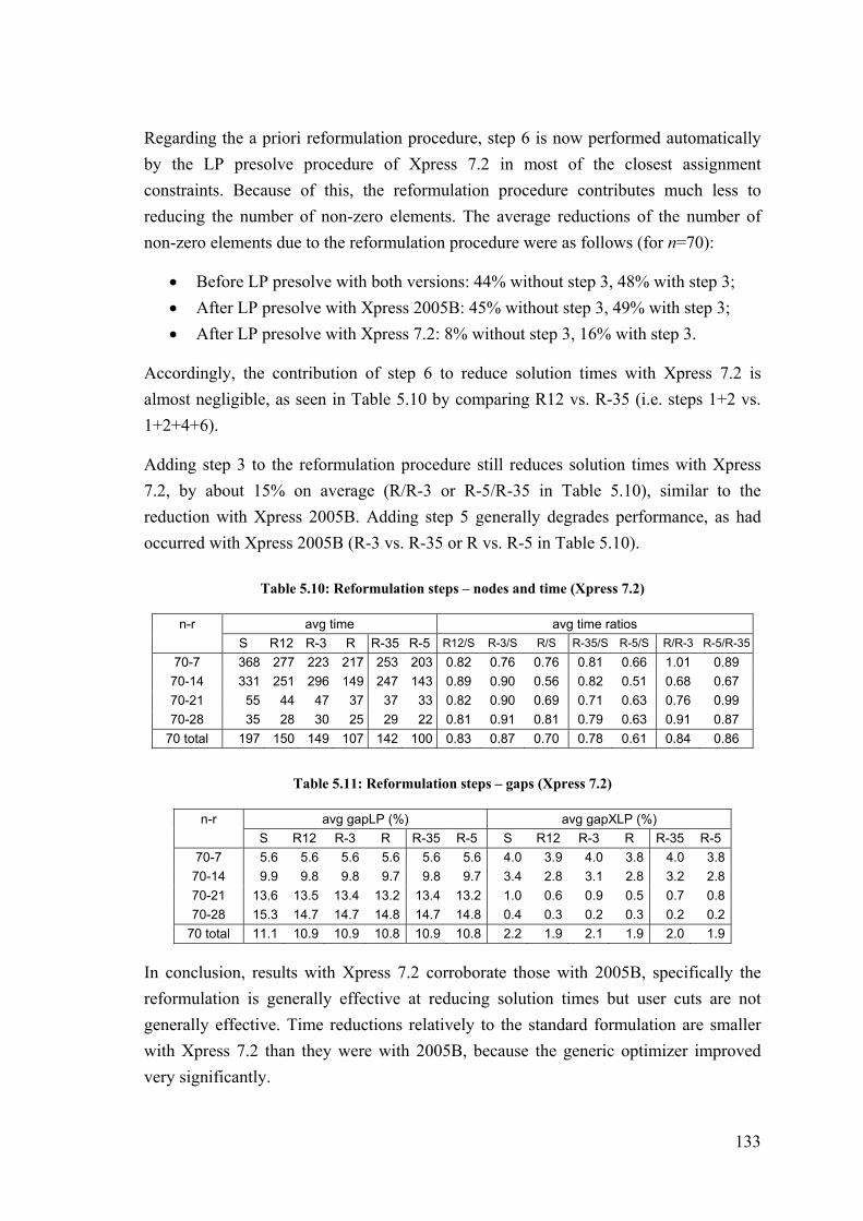
133

Regarding the a priori reformulation procedure, step 6 is now performed automatically

by the LP presolve procedure of Xpress 7.2 in most of the closest assignment

constraints. Because of this, the reformulation procedure contributes much less to

reducing the number of non-zero elements. The average reductions of the number of

non-zero elements due to the reformulation procedure were as follows (for n=70):

Before LP presolve with both versions: 44% without step 3, 48% with step 3;

After LP presolve with Xpress 2005B: 45% without step 3, 49% with step 3;

After LP presolve with Xpress 7.2: 8% without step 3, 16% with step 3.

Accordingly, the contribution of step 6 to reduce solution times with Xpress 7.2 is

almost negligible, as seen in Table 5.10 by comparing R12 vs. R-35 (i.e. steps 1+2 vs.

1+2+4+6).

Adding step 3 to the reformulation procedure still reduces solution times with Xpress

7.2, by about 15% on average (R/R-3 or R-5/R-35 in Table 5.10), similar to the

reduction with Xpress 2005B. Adding step 5 generally degrades performance, as had

occurred with Xpress 2005B (R-3 vs. R-35 or R vs. R-5 in Table 5.10).

Table 5.10: Reformulation steps – nodes and time (Xpress 7.2)

n-r avg time avg time ratios

S R12 R-3 R R-35 R-5 R12/S R-3/S R/S R-35/S R-5/S R/R-3 R-5/R-35

70-7 368 277 223 217 253 203 0.82 0.76 0.76 0.81 0.66 1.01 0.89

70-14 331 251 296 149 247 143 0.89 0.90 0.56 0.82 0.51 0.68 0.67

70-21 55 44 47 37 37 33 0.82 0.90 0.69 0.71 0.63 0.76 0.99

70-28 35 28 30 25 29 22 0.81 0.91 0.81 0.79 0.63 0.91 0.87

70 total 197 150 149 107 142 100 0.83 0.87 0.70 0.78 0.61 0.84 0.86

Table 5.11: Reformulation steps – gaps (Xpress 7.2)

n-r avg gapLP (%) avg gapXLP (%)

S R12 R-3 R R-35 R-5 S R12 R-3 R R-35 R-5

70-7 5.6 5.6 5.6 5.6 5.6 5.6 4.0 3.9 4.0 3.8 4.0 3.8

70-14 9.9 9.8 9.8 9.7 9.8 9.7 3.4 2.8 3.1 2.8 3.2 2.8

70-21 13.6 13.5 13.4 13.2 13.4 13.2 1.0 0.6 0.9 0.5 0.7 0.8

70-28 15.3 14.7 14.7 14.8 14.7 14.8 0.4 0.3 0.2 0.3 0.2 0.2

70 total 11.1 10.9 10.9 10.8 10.9 10.8 2.2 1.9 2.1 1.9 2.0 1.9

In conclusion, results with Xpress 7.2 corroborate those with 2005B, specifically the

reformulation is generally effective at reducing solution times but user cuts are not

generally effective. Time reductions relatively to the standard formulation are smaller

with Xpress 7.2 than they were with 2005B, because the generic optimizer improved

very significantly.

135

5.11 Appendix – Closest assignment constraints

1. Introduction

Some location models require closest assignment (CA) constraints or equivalent

preference constraints – applications are discussed by Hanjoul and Peeters (1987) and

by Gerrard and Church (1996).

In this text, we provide recommendations on selecting a formulation of CA constraints,

among the several alternatives proposed in the literature, regarding expected

computational performance with a generic MIP optimizer. For this purpose, we consider

five commonly used alternative formulations, summarize previous results on their

properties (including strength of LP relaxations), and report on computational

experiments with the CM model.

Note: When a first version of this text was written, it contributed to previous literature

with a comparison between the CA constraints denoted (WBR) below, which is adopted

in some recent articles, with previous alternatives. However, Espejo et al. (2012)

published a recent article providing a comprehensive comparison of CA constraints,

including the contribution above and additional new results. Thus, this text loses some

relevance, but it was still kept in the thesis (although revised to consider the results of

that recent article) since it contains computational results and additional

recommendations, complementing previous literature.

2. Formulations

The notation used here is the same as before: I and J are the sets of centers and sites,

respectively, yj are the location variables, xij are the assignment variables, dij are the

distances between centers and sites. We also introduce the following notation for

demand and variable upper bound constraints used in location models:

1ijj J

x

, i I (D=)

1ijj J

x

, i I (D)

ij jx y , ,i I j J (V)

136

We will consider the following two feasible sets of locations models:

={0,1} , {0,1} : (D ); (V); (CA)nm mX x y

{0,1} , {0,1} : (D ); (V); (CA)nm mX x y

where (CA) denotes a formulation of CA constraints stating that each center cannot be

assigned to a facility farther than the closest open facility (determined by dij data). In set

X , all centers must be fully served by a single, closest facility. In set X , centers may

be either fully served from a single, closest facility or not served by any facility. The

definition of CA constraints above is compatible with both sets, as it allows centers not

to be served.

It is useful to distinguish the two sets because both arise in location problems studied in

the literature. Note that CA constraints valid for these sets are also valid for restrictions

of them, considering e.g. capacity constraints or a fixed number of facilities. We

introduce notation for particular restrictions that will be useful later:

pX : denotes a restriction of X with the additional constraint jj J y p ,

with p being a parameter.

In Table 5.12, we cite references studying models with different feasible sets. For set

X and restrictions of it, the list is not exhaustive of the literature. For set X and

restrictions of it, no additional references are known to the author, particularly none are

known for set pX .

Table 5.12: References to location models with different feasible sets including CA constraints

Without capacity constraints With capacity constraints

X Hanjoul and Peeters (1987) Carreras and Serra (1999),

Berman et al. (2006)

pX Belotti et al. (2007),

Scaparra and Church (2008)

Kalcsics et al. (2002),

Berman et al. (2009)

X Wagner and Falkson (1975) Vedat and Verter (2002),

Smith et al. (2009)

In formulations below, we retain the notation used before for sets of not farther sites,

equidistant sites, and strictly closer sites, as follows: |ij ik ijN k J d d ,

|ij ik ijE k J d d , \ |ij ij ij ik ijN N E k J d d .

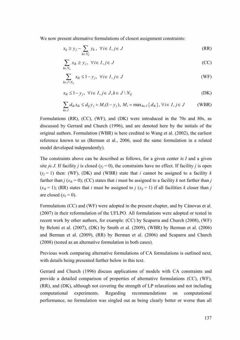
137

We now present alternative formulations of closest assignment constraints:

ij

ij j kk N

x y y

, ,i I j J (RR)

ij

ik jk N

x y

, ,i I j J (CC)

\

1ij

ik jk J N

x y

, ,i I j J (WF)

1ik jx y , , , \ iji I j J k J N (DK)

(1 )ik ik ij j i jk J

d x d y M y

, maxi k J ikM d , ,i I j J (WBR)

Formulations (RR), (CC), (WF), and (DK) were introduced in the 70s and 80s, as

discussed by Gerrard and Church (1996), and are denoted here by the initials of the

original authors. Formulation (WBR) is here credited to Wang et al. (2002), the earliest

reference known to us (Berman et al., 2006, used the same formulation in a related

model developed independently).

The constraints above can be described as follows, for a given center iI and a given

site jJ. If facility j is closed (yj = 0), the constraints have no effect. If facility j is open

(yj = 1) then: (WF), (DK) and (WBR) state that i cannot be assigned to a facility k

farther than j (xik = 0); (CC) states that i must be assigned to a facility k not farther than j

(xik = 1); (RR) states that i must be assigned to j (xij = 1) if all facilities k closer than j

are closed (yk = 0).

Formulations (CC) and (WF) were adopted in the present chapter, and by Cánovas et al.

(2007) in their reformulation of the UFLPO. All formulations were adopted or tested in

recent work by other authors, for example: (CC) by Scaparra and Church (2008), (WF)

by Belotti et al. (2007), (DK) by Smith et al. (2009), (WBR) by Berman et al. (2006)

and Berman et al. (2009), (RR) by Berman et al. (2006) and Scaparra and Church

(2008) (tested as an alternative formulation in both cases).

Previous work comparing alternative formulations of CA formulations is outlined next,

with details being presented further below in this text.

Gerrard and Church (1996) discuss applications of models with CA constraints and

provide a detailed comparison of properties of alternative formulations (CC), (WF),

(RR), and (DK), although not covering the strength of LP relaxations and not including

computational experiments. Regarding recommendations on computational

performance, no formulation was singled out as being clearly better or worse than all

138

others for all models. However, the authors emphasized that (RR) was the most widely

cited and has a particular property (redundancy of VUB constraints) offering a potential

computational advantage.

More recently, Espejo et al. (2012) provide an updated and thorough comparison of

alternative CA formulations including all the commonly used ones: (CC), (WF), (RR),

(DK), (WBR) (or BDTW in their notation), (C2) (or CGLM in their notation, the

inequalities proposed by Cánovas et al. (2007) that generalize (WF) and were presented

before in this chapter), and four additional formulations valid for set pX but not for

X . The authors provide a complete analysis of formulation strength, allowing any two

CA formulations to be compared, and give formal proofs of properties previously noted

by Gerrard and Church (1996). Regarding recommendations on computational

performance, the authors favor two formulations leading to the strongest LP relaxations

(as detailed further below). However, computational experiments are not reported.

Note: In the present text we do not analyze some of the CA formulations above: (C2)

because it requires O(n3) constraints; the four formulations dedicated to set pX

because they are not valid for the more general set X .

Before the previous article, the strength of LP relaxations of the UFLPO with

alternative CA formulations had been compared by Hanjoul and Peeters (1987) and by

Hansen et al. (2004), as detailed below.

Computational experiments comparing alternative CA formulations have rarely been

reported. In experiments with particular models and using a generic MIP optimizer,

Scaparra and Church (2008) compared (CC) and (RR), and Berman et al. (2006)

compared (WBR) and (RR). In both cases, (RR) was found to perform worse.

3. Properties

All the alternative formulations of CA constraints presented above lead to equivalent

definitions of set X . However, they differ on suitability for different model and data

assumptions, and on other properties influencing computational performance.

Suitability for models with different demand constraints: For models

requiring all centers to be assigned (set X ), all CA formulations above are

valid. For models allowing centers not to be assigned (set X ), only (WF), (DK)

and (WBR) are valid. Formulations (CC) and (RR), even if demand constraints

are relaxed from “=” to “≤”, force all centers to be assigned when at least one

facility is open.

139

Suitability for data with distance ties: All CA formulations above, except

(RR), are valid when data has distance ties, i.e. dij = dih for a center i and distinct

sites j and h. If a center has two or more equidistant closest facilities, then it can

be assigned to any one of them. On the other hand, (RR) is not generally valid

with distance ties, as it rules out some feasible solutions: if two or more

equidistant facilities were the closest, then (RR) would require full assignment

to each of them; therefore at most one can be open. Generalizations of (RR) to

deal with distance ties are presented in a section below.

Formulation size: (DK) and (WBR) have disadvantages in terms of formulation

size. All CA formulations above require O(n2) constraints, except (DK) which

requires O(n3). Formulation (WBR) requires a larger number of non-zero

elements than (RR), (CC), and (WF), as the first involves all sites k J in all

constraints, while the others involve only a subset.

Formulation strength: The alternative CA formulations lead to models with

different LP relaxations. This is discussed in the next section.

Property of single assignment: All CA formulations above have the property

that they suffice to guarantee single assignment in the definition of set X , that

is, if all variables y take 0-1 binary values, variables x will also take 0-1 binary

values, even if they are defined as continuous. However, this applies only to

pairs (i, j) without distance ties (Eij={j}); for pairs (i, j) with distance ties

(|Eij|>1), all CA formulations (except (RR), as noted above) allow demand to be

freely distributed among equidistant, closest facilities with fractional

assignments. Thus, this property allows reducing the number of integer variables

in the formulation of X .

Property of redundancy of constraints (V): Formulation (RR) has the property

that constraints (V) are redundant in the definition of set X restricted to at least

one open facility ( 1jj J y ), e.g. to set pX . That is, if all variables y take

binary values 0-1, constraints (V) are automatically satisfied. Thus, constraints

(V) may be dropped, giving a smaller but still valid integer formulation of X ,

although leading to a weaker LP relaxation. The other formulations do not have

this property.

All of the properties above were noted in the literature before, particularly in the

thorough discussions by Gerrard and Church (1996) and Espejo et al. (2012). Here we

provide only a compact summary and clarify the suitability for sets X and X

140

(Gerrard and Church (1996) discussed both sets but did not include (WBR), Espejo et

al. (2012) included (WBR) but focused on sets X and pX ).

4. Formulation strength

In the text below, given alternative formulations A and B of CA constraints valid for a

set X formulated with integer variables, A is said to dominate B if the continuous

relaxations of X defined with A and B, denoted PA and PB, are such that PA PB. In this

case, A leads to stronger LP relaxations of problems with feasible set X, i.e. providing

bounds at least as tight.

The strength of LP relaxations of the UFLPO (which has feasible set X ) with

alternative CA formulations was discussed by Hanjoul and Peeters (1987), who note

that (CC) dominates (RR), and by Hansen et al. (2004), who show that (CC) and (WF)

are equivalent and dominate (DK) and (RR). Here we summarize these results and also

analyze (WBR). We assume the feasible integer set is X unless otherwise noted.

(WF) is equivalent to (CC): It is immediate to verify that one formulation can be

converted into the other using demand constraints 1ijj J x for i I .

(CC) dominates (RR): We assume there are no distance ties. For a given (i, j), (RR)

can be re-written as

ij

j ij kk N

y x y

.

Combining (CC) and (V), we get

ij ij ij

j ik ij ik ij kk N k N k N

y x x x x y

.

Thus, (CC) implies (RR) if constraints (V) hold. The converse is not true, as shown by

the following example. Given a center i and sites 1, 2, 3, 4 in increasing distance to i,

the point y1=y2=0.5, y3=y4=1, xi1=0.5, xi2=xi3=0 and xi4=0.5 satisfies (RR) for j=1, 2, 3, 4,

but violates (CC) for j=3.

(WF) dominates (DK): It is immediate to verify that (WF) implies (DK) in the forms

given above, as the left-hand side of (WF) is greater than or equal to the one of (DK).

The converse is not true, as shown by the following example. Given a center i and sites

1, 2, 3 in increasing distance to i, the point y1=y2=y3=0.5, xi1=0, xi2=xi3=0.5 satisfies

(DK) but violates (WF) for j=1.

141

(WF) dominates (WBR): We assume 0i ijM d for all i and j. For a given (i, j),

(WBR) can be re-written as follows, by separating the sum over set J:

\

(1 )ij ij

ik ik ik ik ij j i jk N k J N

d x d x d y M y

.

Now considering that demand constraints imply

\

1ij ij

ik ikk N k J N

x x

and that constraints (WF) are

\

1ij

ik jk J N

x y

,

summing the first multiplied by ijd with the second multiplied by i ijM d , we get:

\

1ij ij

ij ik i ik ij j i jk N k J N

d x M x d y M y

.

This inequality dominates (WBR) as, in the left-hand sides, ik ijd d for ijk N and

ik id M for \ ijk J N . Thus, (WF) implies (WBR) if demand constraints hold. The

converse is not true, as shown by the following example. Given a center i and sites 1, 2,

3 such that di1=1, di2=2, di3=3, Mi=3, the point y1=0.5, y2=y3=1, xi1=0.5, xi2=0 and

xi3=0.5 satisfies (WBR) for j=1, 2, 3, but violates (WF) for j=2.

The arguments above also show that (WF) dominates (DK) and (WBR) in the case of

feasible set X .

Espejo et al. (2012) show in addition that (DK) dominates (WBR). They also show

through particular examples that no domination relation exists between (RR) and

(WBR), or between (RR) and (DK). They also analyze the strength of four additional

CA formulations valid for set pX .

5. Generalizations of (RR) to deal with distance ties

Here we propose the following generalization of (RR) to deal with distance ties, which

was also proposed by Espejo et al. (2012):

ij ij

ik j kk E k N

x y y

, ,i I j J (RR2)

If Eij ={j}, (RR2) reduces to (RR). If |Eij|>1, (RR2) states that if facility j is open and all

strictly closer facilities are closed then i must be assigned to j or to an equidistant site

(kEij). These constraints now work properly if more than one facility in Eij is open. We

note that (CC) dominates (RR2), by a similar argument as used above for (RR).

142

Other generalizations of (RR) to deal with distance ties have been proposed:

\

1

| |ij ij

ik k k kk S k S k N k E S

x y y yS

, , ii I j J , ijS E (RR3)

1

ij ij ij

ik k kijk E k E k N

x y yE

, , ii I j J (RR4)

Formulation (RR3) was proposed by Gerrard and Church (1996), who call it MAC1,

and (RR4) was proposed by Berman et al. (2006). The set Ji contains only one element

from each distinct set Eik for kJ. For a given (i, j) such that |Eij|>1, (RR2) requires |Eij|

constraints, while (RR3) requires a higher number (e.g. 3 constraints if |Eij|=2, 7

constraints if |Eij|=3), and (RR4) requires only one – actually, (RR4) corresponds to

(RR3) written only for maximal sets S = Eij. Gerrard and Church (1996) note that

(RR3), like the original (RR), remains valid if (V) are dropped from the model. On the

other hand, we note that (RR2) and (RR4) require (V) or equivalent constraints

forbidding assignments to closed facilities for pairs (i, j) such that |Eij|>1.

We note that (RR2) dominates (RR3): summing (RR2) for all j S and dividing by |S|,

an expression is obtained that dominates (RR3) if (V) holds. (RR2) also dominates

(RR4): summing (RR2) for all ijj E and dividing by |Eij|, (RR4) is obtained. Thus,

(RR2) leads to stronger LP relaxations than the other generalizations, and in our

computational experiments we considered only (RR2).

6. Computational experiments with the CM model

Four formulations of the CM model were tested: CC denotes our standard formulation

(5.1)-(5.8) and (5.9), which uses CA formulation (CC); WBR, RR, DK denote

formulations where (CC) was replaced by (WBR), (RR2) and (DK), respectively.

Note: In addition to the formulations above, we did preliminary experiments with a

variant of RR without constraints (V), obtained by: using (RR2) instead of (CC),

dropping (V) for all pairs (i, j) such that |Eij|=1, and adding the constraint 1jj J y (at

least one open facility). This formulation had a very weak initial LP relaxation,

violating many constraints (V) and even many of the weaker constraints ij ji I x n y

for j J , and a very large time was required even for generating cuts at the top node.

Thus, this formulation was dropped from consideration.

Instances of sizes n=50 and n=70 were tested, generated as described before. All

instances have a significant number of distances ties.

143

Results were obtained for two versions of the Xpress solver: 2005B (MIP Optimizer

16.10) and 7.2 (MIP Optimizer 22.01). We show results with the two versions because

some interesting observations can be made regarding the evolution of different solver

components. Solution times are comparable between the two versions since the same

computer was used, as described before. The time limit was set to 1 hour and solver

parameters were set as before: branching priority was given to variables y; other

parameters were left at default values.

The results reported below are the same as before and additionally:

time XLP: time (in seconds) spent in cut generation and heuristics at the top

node;

htop gap 0%: number of instances where heuristics at the top node found an

optimal solution (whether or not optimality was proven at the top node);

htop gap 5%: number of instances where heuristics at the top node found a

feasible solution with a value within 5% of the optimal value;

Note: Results for DK with n=70 are not reported since cut generation at the top node

required more than the physical memory available in the computer used.

Note: Some of the results below, regarding solver components such as presolve, cut

generation and heuristics, were surprising. Explaining such results is not always

immediate, given that the operation of solver components is not fully documented.

Formulation size (Table 5.13)

Formulations CC and RR have the same number of non-zero elements before LP

presolve, and WBR has many more (each CA constraint involves all sites, not only the

closer or equidistant sites). LP presolve in Xpress 7.2 significantly reduces the number

of non-zero elements of CC and WBR. With CC, it performs an equivalent

simplification to step 6 of the reformulation procedure presented before. With WBR, it

is even more effective than with CC. This latter result was surprising, but was not

analyzed further.

DK is much larger than CC and RR (it has n3 CA constraints instead of n2). LP presolve

in Xpress 2005B performs a large reduction of the model, while Xpress 7.2 reduces it

only slightly (for reasons that are unclear).

144

Table 5.13: Formulation size (n=50, average for all capacity ratios r)

LP presolve CC WBR RR DK

rows before 5 101 5 101 5 101 63 190

after - Xpress 2005B 4 947 5 047 5 001 21 092

after - Xpress 7.2 4 947 5 047 5 001 60 639

non-zero before 77 011 135 046 77 011 131 277

elements after - Xpress 2005B 74 030 132 422 76 761 89 179

after - Xpress 7.2 46 269 44 962 76 760 128 727

Solution time (Table 5.14)

Solution times are lowest with CC and WBR, and are much higher with RR and DK, by

a factor of 5 or more (considering RR/CC for size n=70, DK/CC for size n=50, and any

of the solver versions).

Comparing CC with WBR, using Xpress 2005B, CC is solved faster than WBR for all

instance groups, except for n-r = 70-14 (note: the time ratio WBR/CC is 1.0 even

though WBR has lower average time than CC; this is due to the fact that the best

formulation varies for individual instances). Using Xpress 7.2, CC is solved faster than

WBR for smaller capacity ratios and slower for larger capacity ratios; although the

global average time ratio WBR/CC is 1.0 for n=70, CC can be considered more

effective as it is solved faster for instances with lower capacity ratios, which are harder.

As noted before, Xpress 7.2 is much faster than 2005B. The improvement occurs for all

formulations (except for DK, which performs worse, for reasons that are unclear).

LP and XLP gaps (Table 5.14)

The LP gaps of CC are the lowest, as expected. The difference relative to other

formulations is small for smaller capacity ratios and increases for larger ones.

However, it turns out that the XLP gaps of CC are not the lowest: they are generally the

highest among all formulations with Xpress 2005B; they are only the second lowest

with Xpress 7.2. In both Xpress versions, WBR consistently has the lowest gaps across

all capacity ratios. These results were surprising, but their causes were not analyzed

further, particularly which cut types are responsible for closing the XLP gap of WBR

(this task is made difficult since Xpress logs do not discriminate the types of added

cuts).

145

Table 5.14: Main results (n=50 and 70)

Xpress 2005B Xpress 7.2 total finished n-r CC WBR RR DK CC WBR RR DK 50-5 9 9 9 9 9 9 9 9 50-10 9 9 9 9 9 9 9 9 50-15 9 9 9 9 9 9 9 9 50-20 9 9 9 9 9 9 9 9 50 total 36 36 36 36 36 36 36 36 70-7 9 9 6 - 9 9 8 - 70-14 8 9 2 - 9 9 4 - 70-21 9 9 6 - 9 9 9 - 70-28 9 9 9 - 9 9 9 - 70 total 35 36 23 - 36 36 30 -avg time n-r CC WBR RR DK CC WBR RR DK 50-5 28 56 68 87 32 35 58 188 50-10 52 67 183 146 33 26 116 242 50-15 43 51 153 127 22 15 75 189 50-20 9 19 31 65 10 7 10 98 50 total 33 48 109 106 24 21 65 179 70-7 661 988 1838 - 368 450 1135 - 70-14 1771 1347 2996 - 331 360 2554 - 70-21 241 250 1650 - 55 38 473 - 70-28 64 98 768 - 35 23 116 - 70 total 685 671 1813 - 197 218 1070 -avg time ratios n-r CC WBR RR DK CC WBR RR DK 50-5 1.0 1.8 1.9 5.3 1.0 1.8 1.7 16.6 50-10 1.0 1.6 3.3 3.5 1.0 0.8 3.3 8.4 50-15 1.0 1.5 3.1 3.6 1.0 0.7 3.0 8.3 50-20 1.0 2.3 3.5 9.3 1.0 1.0 1.2 12.0 50 total 1.0 1.8 2.9 5.4 1.0 1.1 2.3 11.3 70-7 1.0 2.3 2.5 - 1.0 1.2 2.6 - 70-14 1.0 1.0 3.1 - 1.0 1.2 8.3 - 70-21 1.0 1.6 6.9 - 1.0 0.7 6.3 - 70-28 1.0 2.0 9.4 - 1.0 0.8 3.0 - 70 total 1.0 1.7 5.5 - 1.0 1.0 5.1 -avg gapLP (%) n-r CC WBR RR DK CC WBR RR DK 50-5 4.6 4.6 4.6 4.7 4.6 4.6 4.6 4.8 50-10 10.2 10.2 10.3 10.3 10.2 10.2 10.3 10.3 50-15 16.1 16.3 16.2 16.3 16.0 16.3 16.0 16.3 50-20 14.5 20.9 14.9 20.7 14.1 20.8 14.4 20.8 50 total 11.3 13.0 11.5 13.0 11.2 13.0 11.3 13.0 70-7 5.6 5.6 5.6 - 5.6 5.6 5.6 - 70-14 9.9 9.9 10.0 - 9.9 9.9 10.0 - 70-21 13.7 13.9 13.8 - 13.6 13.8 13.8 - 70-28 15.5 21.3 15.9 - 15.3 21.2 15.6 - 70 total 11.2 12.7 11.3 - 11.1 12.7 11.2 -avg gapXLP (%) n-r CC WBR RR DK CC WBR RR DK 50-5 3.9 2.8 3.5 3.1 3.0 2.8 3.4 3.1 50-10 6.2 3.3 5.3 4.1 1.9 1.8 3.0 2.4 50-15 6.1 2.9 4.9 3.9 0.9 0.7 2.1 0.7 50-20 3.3 1.4 2.5 3.0 0.0 0.1 0.2 0.2 50 total 4.9 2.6 4.1 3.5 1.4 1.3 2.2 1.6 70-7 4.8 3.9 4.7 - 4.0 3.7 4.5 - 70-14 6.4 3.9 5.9 - 3.4 3.1 4.2 - 70-21 4.4 2.1 4.2 - 1.0 0.6 1.5 - 70-28 3.1 1.4 4.0 - 0.4 0.2 0.6 - 70 total 4.7 2.8 4.7 - 2.2 1.9 2.7 -

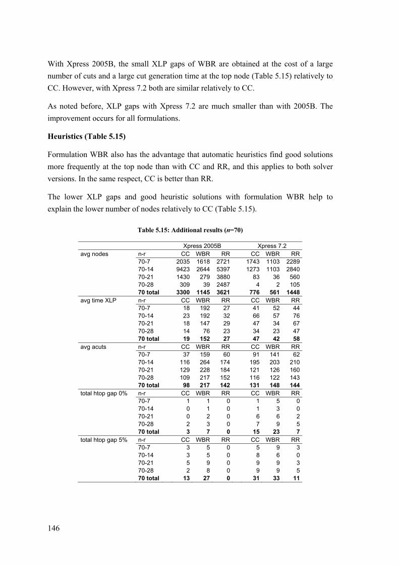
146

With Xpress 2005B, the small XLP gaps of WBR are obtained at the cost of a large

number of cuts and a large cut generation time at the top node (Table 5.15) relatively to

CC. However, with Xpress 7.2 both are similar relatively to CC.

As noted before, XLP gaps with Xpress 7.2 are much smaller than with 2005B. The

improvement occurs for all formulations.

Heuristics (Table 5.15)

Formulation WBR also has the advantage that automatic heuristics find good solutions

more frequently at the top node than with CC and RR, and this applies to both solver

versions. In the same respect, CC is better than RR.

The lower XLP gaps and good heuristic solutions with formulation WBR help to

explain the lower number of nodes relatively to CC (Table 5.15).

Table 5.15: Additional results (n=70)

Xpress 2005B Xpress 7.2 avg nodes n-r CC WBR RR CC WBR RR 70-7 2035 1618 2721 1743 1103 2289 70-14 9423 2644 5397 1273 1103 2840 70-21 1430 279 3880 83 36 560 70-28 309 39 2487 4 2 105 70 total 3300 1145 3621 776 561 1448 avg time XLP n-r CC WBR RR CC WBR RR 70-7 18 192 27 41 52 44 70-14 23 192 32 66 57 76 70-21 18 147 29 47 34 67 70-28 14 76 23 34 23 47 70 total 19 152 27 47 42 58 avg acuts n-r CC WBR RR CC WBR RR 70-7 37 159 60 91 141 62 70-14 116 264 174 195 203 210 70-21 129 228 184 121 126 160 70-28 109 217 152 116 122 143 70 total 98 217 142 131 148 144 total htop gap 0% n-r CC WBR RR CC WBR RR 70-7 1 1 0 1 5 0 70-14 0 1 0 1 3 0 70-21 0 2 0 6 6 2 70-28 2 3 0 7 9 5 70 total 3 7 0 15 23 7 total htop gap 5% n-r CC WBR RR CC WBR RR 70-7 3 5 0 5 9 3 70-14 3 5 0 8 6 0 70-21 5 9 0 9 9 3 70-28 2 8 0 9 9 5 70 total 13 27 0 31 33 11

147

7. Conclusion

Our computational experiments with the CM model can be summarized as follows:

formulation (CC) was the most efficient, (WBR) was competitive (with Xpress 7.2),

while (RR) and (DK) had much higher solution times (by a factor of 5 or more).

In our experiments, we also observed that the relative performance of formulations can

be influenced not only by the strength of the initial LP relaxation but also by the effect

of the several components of a generic branch-and-cut solver, such as presolve, cut

generation and heuristics. Indeed, our results with formulation (WBR) were surprising:

the number of non-zero elements was the smallest after LP presolve (while it was the

largest before) in Xpress 7.2; the LP gap after adding cuts at the top node was smaller

than with (CC) (while it was larger before); heuristic solutions at the top node were

better or found more frequently than with all other formulations. Thus, for models other

than CM, or with other solvers, it may also be worthwhile trying (WBR).

The performance of alternative formulations of CA constraints may vary for different

location models, depending e.g. on the type of objective function and on the presence of

minimum and/or maximum capacity constraints. Nevertheless, on the basis of previous

results in the literature and of our work in this chapter, we can offer some general

observations and recommendations.

First, we observe that (DK) should not be used since it is clearly dominated by (WF).

Both have the flexibility of being applicable to X in addition to X , but (DK) leads to

a weaker and much larger formulation. In our experiments with the CM model, (DK)

had clearly the worst performance of all formulations.

We start with recommendations for solving a standard formulation with a generic MIP

optimizer, without additional development effort. For models with feasible set X (or a

restriction of it):

All the formulations (CC), (WF), (WBR), (RR), and (DK) are applicable.

(CC) or its equivalent (WF) should be the first choice, as it leads to a stronger

LP relaxation, while not requiring a larger formulation. It performed best in our

experiments with the CM model.

(WBR) may also be worthwhile to try. Even though (WBR) seems a poor choice

relatively to (CC), because the initial formulation is weaker and has more non-

zero elements, in practice it can perform well, as shown in our experiments on

the CM model with Xpress 7.2.

148

(RR) (and its generalization (RR2) to deal with distance ties) is less promising,

as it leads to a weaker LP relaxation than (CC) and was found to perform worse

in some particular models. In our experiments with the CM model, it performed

significantly worse than (CC). In previous experiments with particular models,

Scaparra and Church (2008) and Berman et al. (2006) found that (RR)

performed worse than (CC) and (WBR), respectively.

(DK) should not be used, as noted above.

For set pX (which is a restriction of X , so all the above applies), it may also

be worthwhile to experiment with the new formulation EMR of CA constraints

proposed by Espejo et al. (2012). This formulation also has O(n2) constraints

and is not dominated by (CC) (nor dominates it). No computational results have

been reported with this formulation.

For models with feasible set X (or a restriction of it still allowing centers not to be

assigned to any facility):

Only formulations (WF), (WBR), (DK) are applicable.

(WF) should be the first choice, as it leads to the strongest LP relaxation.

(WBR) may also be worthwhile to try; however, as far as we know, no previous

experiments have been reported.

(DK) should not be used, as noted above.

We now comment on using the a priori reformulation procedure proposed in this

chapter, based on a previous one by Cánovas et al. (2007). For models with feasible set

X :

This procedure is recommended since it requires only moderate implementation

effort and reduces solution times significantly, according to our experiments and

those of Cánovas et al. (2007).

Steps 1-4 can be used with all CA formulations considered here. Note that steps

1, 2, 3.1, and 4 are valid with any constraints that enforce CA. Step 3.2 (drop

CA constraints made redundant by equalities (Weq) added in step 3.1) was

shown to be valid for (WF). Since constraints (WF) dominate the alternative

constraints considered here, step 3.2 can also be applied to the latter.

For set pX using formulation EMR, step 3.2 may no longer apply or may

weaken the formulation, since (WF) does not dominate EMR (Espejo et al.,

2012). We did not further analyze this issue.

Steps 5-6 apply only to formulations (WF) and (CC).

149

For models with feasible set X :

Only step 5 is valid for set X , and only if formulation (WF) is used. No

computational results have been reported for this case. The other steps rely on

inequalities that are valid only when all centers must be assigned (demand

constraints hold with “=”).

Finally, we offer some comments on other recommendations in the literature:

Relax the integrality of variables x: All CA formulations allow the integrality

of variables x to be relaxed in the definition of set X (for pairs (i, j) without

distance ties). Gerrard and Church (1996) and Espejo et al. (2012) suggest that

such reduction in the number of integer variables might improve the

performance of a branch-and-bound algorithm, but no computational results are

offered or cited.

In our experiments, we chose to leave variables x defined as binary and to give

branching priority to variables y (the rationale is that assignments are subsidiary

to location decisions, especially when CA applies). This priority suffices to

render variables x innocuous for the branch-and-bound tree (except when

equidistant closest facilities occur), and indeed significantly reduced solution

times, as noted before in this chapter. Additionally, leaving variables x defined

as binary may be useful to help reduce or tighten the formulation through

automatic presolve and cut generation procedures relying on that information.

However, we did not perform experiments with continuous variables x to verify

whether performance was improved or degraded.

Drop constraints (V) when using (RR): Formulation (RR) allows constraints

(V) to be dropped from the definition of set X (restricted to guarantee at least

one open facility), although at the cost of a weaker LP relaxation. Gerrard and

Church (1996) suggest that reducing model size by dropping all or a subset of

(V) might improve computational performance, but no computational results are

offered or cited.

We observe that this approach does not seem very promising in general, since it

is well known that constraints (V) are crucial to strengthen the formulations of

many location models. That is, dropping (V) will likely only improve

performance for particular models in which the objective function and

constraints other than (V) and (RR) promote LP solutions that naturally tend to

satisfy (V). In those cases, all CA formulations may also perform better if (V) is

150

replaced by the weaker but smaller set of constraints ij ji I x n y for j J . In

the case of the CM model, dropping (V) leads to very weak LP relaxations and

degrades performance very significantly, as verified in experiments described

above.

Other CA formulations: In the conclusion of their recent article, Espejo et al.

(2012) focus their recommendations on using formulations providing the tightest

LP relaxations. The authors suggest using (C2) instead of (WF) but restricted to

O(n2) constraints (by picking a single additional center for each pair of centers

and sites), which would still provide a tighter formulation. For set pX , the

authors suggest using (C2) as above, or the new formulation EMR proposed by

the authors (which also requires O(n2) constraints, and is neither dominated by

nor dominates (C2)), or both in conjunction with one set of constraints included

a priori and the other set used to generate cuts. The authors leave

implementation details and experiments to future work. Thus, while these

approaches may be computationally effective, they have not been tested before.

151

Chapter 6

Solving facility location models with modern

optimization software: the weak and strong

formulations revisited

6.1 Introduction

The classic fixed-charge facility location problems – uncapacitated, capacitated, and

capacitated with single-sourcing, denoted UFLP, CFLP and CFLPSS, respectively –

consider decisions of locating facilities (such as plants or warehouses in supply chain

networks or concentrators in telecommunications networks) in a discrete set of potential

sites and assigning discrete demand centers to those facilities, with the objective of

minimizing the total costs of satisfying all demand, composed of fixed costs of

installing facilities and variable costs of operation and transportation. Formulations,

model extensions, solution methods and applications are reviewed by Klose and Drexl

(2005) and Gourdin et al. (2002).

Right from the first studies of these models, the so-called weak and strong variants of

mixed-integer linear programming (MIP) formulations have been considered, differing

in the constraints linking assignment and location variables, and involving a trade-off

between model size and linear programming (LP) relaxation bounds. For the UFLP, it is

well known that, for many instances of practical interest, the LP relaxation of the strong

formulation gives integer or close to integer solutions, requiring no or very few

additional nodes of branch-and-bound (Krarup and Pruzan, 1983). The same happens

with other uncapacitated location models, such as the p-median problem (ReVelle,

1993). Capacitated models such as the CFLP are harder to solve, but still the strong

formulation produces smaller LP gaps (Cornuejols et al., 1991). Although many early

LP-based branch-and-bound algorithms were based on the weak formulation (Sridharan,

1995), the strong formulation of the CFLP is used frequently by several authors

proposing different solution approaches. These include branch-and-cut (Aardal, 1998b;

Avella and Boccia, 2009) and Lagrangian relaxation (Sridharan, 1995). Díaz and

Fernández (2001) solve the strong formulation of the CFLPSS with a generic MIP

optimizer to provide a benchmark for a specialized exact algorithm.

152

In this chapter we present computational experiments on solving the CFLP and CFLPSS

(and also the UFLP for comparison) with a modern MIP optimizer implementing a

generic branch-and-cut algorithm. The aim is to compare the computational

performance of well-known formulation variants, combining the weak and strong

variants, and additional constraints involving facility capacities that are redundant for

the LP relaxation but help the optimizer recognize certain model relaxations and

generate strong cutting planes, as recommended by Aardal (1998b).

Our empirical investigation is motivated by previous, more restricted computational

experiments done by the authors with the CFLP, where surprisingly the weak

formulation was found to be solved faster than the strong one with a generic MIP

optimizer. Trick (2005) discusses a similar result with a particular instance of the CFLP.

Here we aim to: (i) identify instance data types, including different levels of capacity

and fixed costs, for which the weak formulation may be solved faster than the strong

one; (ii) identify the most effective formulation, among the variants referred to above;

(iii) check whether results for the CFLP also apply to the related CFLPSS, as well as to

an unrelated facility location model, the capacitated median model, which does not

involve fixed location costs and involves minimum rather than maximum capacity

constraints.

We point out that using a generic MIP optimizer, even with the most effective

formulation possible, may not be suitable for every application. There are efficient

specialized algorithms that are able to solve large instances to optimality or near

optimality. Exact algorithms include those of: Körkel (1989) for the UFLP; Avella and

Boccia (2009), Görtz and Klose (2012) for the CFLP; Díaz and Fernández (2001),

Avella et al. (2011) for the CFLPSS. Heuristic algorithms include those of: Barahona

and Chudak (2005) for the UFLP and CFLP; Ahuja et al. (2004) for the CFLPSS.

Nevertheless, our results can be useful to practitioners wishing to solve models

efficiently with minimal modeling effort, or to researchers using a generic MIP

optimizer to provide a benchmark for specialized solution algorithms.

In our experiments we use FICO’s Xpress MIP optimizer. General descriptions of MIP

software implementing branch-and-cut algorithms are given by Atamturk and

Savelsbergh (2005) and Lodi and Linderoth (2011). State-of-the-art commercial MIP

software packages include: Xpress (Ashford, 2007; Laundy et al. 2009), CPLEX (Bixby

et al., 2000; Bixby and Rothberg, 2007), and Gurobi (Bixby, 2011). The references cited

describe the components of MIP solvers and their historical performance evolution.

153

The remainder of this chapter is organized as follows: section 2 addresses fixed-charge

location problems; section 3 addresses the capacitated median model; section 4 offers

overall conclusions.

6.2 Fixed-charge location problems

6.2.1 Formulations

We start by presenting mixed-integer linear programming formulations of the UFLP,

CFLP and CFLPSS. We are given a set of demand centers 1,...,I n , a set of sites

where facilities can be installed 1,...,J m , and the following data, for i I and

j J : id is the demand of center i; js is the maximum capacity of site j; jf is the fixed

cost of installing and operating a facility at site j; ijc is the variable cost of serving all

the demand of center i from site j. Decision variables are: 1jy if a facility is installed

(or open) at site j J , and equals zero otherwise; ijx is the fraction of the demand of

center i I served from site j J .

The uncapacitated facility location problem, UFLP, is the problem of finding which

facilities to open, and assigning centers to those facilities, in order to minimize the total

cost of serving all the demand. Capacities are assumed to be as large as necessary. The

weak formulation of the UFLP is

(W-UFLP):

Min ij ij j ji I j J j J

c x f y

Subject to 1ijj J

x

, i I (D)

ij ji I

x n y

, j J (U)

{0,1}jy , j J (I)

0ijx , ,i I j J (N)

In this formulation and those following, constraints are identified by letters using a

notation similar to the one of Cornuejols et al. (1991). Constraints (D) state that all

demand has to be served. Constraints (U) link x and y variables, and state that if a

facility is open it can serve any number of centers, otherwise no center can be assigned

to it. Expressions (I) and (N) are integrality and non-negativity constraints on variables.

Note that (N) and (D) imply 0 1ijx for all i and j.

154

The m constraints (U) can be replaced with the n m variable upper-bound constraints

ij jx y , ,i I j J (B)

which state that center i can only be served by a facility at j if it is open. By doing this,

we obtain the strong formulation of the UFLP:

(S-UFLP):

Min ij ij j ji I j J j J

c x f y

Subject to (D), (B), (I), (N)

The strong and weak integer formulations are equivalent, i.e. define the same set of

integer solutions. However, their LP relaxations, obtained by replacing (I) with

0 1jy for j J , are not equivalent. Formulation (S-UFLP) is said to be stronger or

tighter, as the set of solutions to its LP relaxation is strictly contained in the one of (W-

UFLP). Moreover, constraints (B) have the property of being facet-defining for the

UFLP polytope (Cornuejols et al., 1990). It is well known that, in many instances of

practical interest, the LP relaxation of (S-UFLP) gives integer or close to integer

solutions, requiring no or very few additional nodes of branch-and-bound (Krarup and

Pruzan, 1983).

The capacitated facility location problem, CFLP, is obtained from the UFLP by

imposing maximum capacities on facilities. Its weak formulation is

(W1-CFLP):

Min ij ij j ji I j J j J

c x f y

Subject to 1ijj J

x

, i I (D)

i ij j ji I

d x s y

, j J (C)

{0,1}jy , j J (I)

0ijx , ,i I j J (N)

where (C) are the capacity constraints. The strong formulation is obtained by adding

constraints (B):

(S1-CFLP):

Min ij ij j ji I j J j J

c x f y

155

Subject to (D), (C), (B), (I), (N)

While constraints (B) are redundant for the integer formulation, they strengthen the LP

relaxation (Cornuejols et al., 1991) and were shown (by Aardal, cited by Avella and

Boccia, 2009) to be facet-defining for the CFLP polytope for all i I and j J such

that i jd s . Constraints (B) can also strengthen Lagrangian relaxations (Cornuejols et

al., 1991; Sridharan, 1995). For these reasons, the strong formulation appears frequently

in the literature, as was noted in the introduction.

Additional redundant constraints have been proposed in the literature, based on

aggregate capacity and demand expressions. They are redundant even for the LP

relaxation, but strengthen Lagrangian relaxations or help branch-and-cut solvers

recognize particular model relaxations for which strong cutting planes can be generated.

First, we recall the total capacity constraint

j j ij J i I

s y d

, (T)

which states that the total capacity of open facilities should cover total demand. Note

that (T) is redundant both for the integer formulation and the LP relaxation of the CFLP,

as it can be obtained from constraints (C) and (D). However, Cornuejols et al. (1991)

show the theoretical and practical advantages of adding (T) to strengthen Lagrangian

relaxations.

Second, we recall the constraint set

j i iji I

z d x

, j J (Z)

j j jz s y , j J (C )

j ij J i I

z d

(F)

0jz , j J (Nz)

where (Z) define auxiliary occupied capacity variables, (C ) replaces (C), and (F)

establishes the flow equilibrium between total occupied capacity and total demand.

Aardal (1998b) proposes a formulation obtained from (S1-CFLP) and using the

constraint set above. While not improving the LP relaxation bound, this formulation

enables a MIP optimizer to recognize the surrogate knapsack set, X K, and the single-

node flow set, X SNF,

156

{0,1} : (T)K mX y

, {0,1} : (F), (C )SNF m mX z R y

and to generate lifted cover cuts and flow cover cuts, developed for X K and X SNF,

respectively, which are facet-defining inequalities for the CFLP polytope under some

conditions (Aardal, 1998b). In the experiments of Aardal, using the MINTO branch-

and-cut solver, significant time reductions were obtained (on average 20-80% for

groups of instances with varying capacity data).

Note that (T) was not explicitly added to the formulation proposed by Aardal, but

presumably it was recognized by MINTO automatically by combining (C ) and (F). In

our experiments using the Xpress solver (described below), we noticed that explicitly

adding (T) as well led to some variation in cut generation (in terms of number of cuts

and LP bound at the top node) and systematically reduced solution time (only slightly or

by up to 30%, both for the weak and strong formulations of the CFLP and CFLPSS

models). For this reason, (T) was also added to the formulation in our experiments.

To summarize, we consider the following CFLP formulation variants:

(W1-CFLP) denotes Min ij ij j ji I j J j Jc x f y , s.t. (D), (C), (I), (N);

(W2-CFLP) denotes (W1-CFLP) with (T) added;

(W3-CFLP) denotes (W1-CFLP) with (C) removed, (Z), (C ) , (F), (Nz) added,

and (T) also added;

(S1-CFLP) denotes (W1-CFLP) with (B) added;

(S2-CFLP) denotes (W2-CFLP) with (B) added;

(S3-CFLP) denotes (W3-CFLP) with (B) added;

We call W1 and S1 the standard formulations, and the others aggregate formulations.

Finally, the CFLPSS is the capacitated facility location problem with single sourcing (or

single assignment), in which each center’s demand cannot be split and must be served

from a single facility. For the UFLP, an optimal solution can be found where variables x

are either zero or one without explicitly requiring them to be integer (Krarup and

Pruzan, 1983). This property does not hold for capacitated models and, if required, must

be enforced with integrality constraints:

0,1ijx , ,i I j J (SS)

We consider six variants of CFLPSS formulations, obtained by replacing (N) with (SS)

in the CFLP formulations above.

157

6.2.2 Instances

The test instances were randomly generated using the procedure of Cornuejols et al.

(1991), which was devised for the CFLP. Their main features include variable costs

depending on Euclidean distances, fixed costs reflecting economies of scale, and

varying capacity levels. We opted for this procedure as these features can be considered

representative of real-world problems and it has been used by several other authors for

benchmarking algorithms for the CFLP, e.g. Aardal (1998b), Barahona and Chudak

(2005), Avella and Boccia (2009), and Görtz and Klose (2012).

The procedure is the following, for a given size n m :

points representing centers and sites are randomly generated in 0,1 0,1 ;

demands id are generated from a uniform distribution 5,35U ;

variable costs are set to 10ij i ijc d e , where ije is the Euclidean distance

between center i and site j;

capacities js are generated from 10,160U ;

fixed costs are generated with the formula 0,90 100,110j jf U U s ;

capacities js are then scaled to obtain instances with different capacity levels

Cap = j ij J i Is d (note that fixed costs are not affected by this scaling).

Cornuejols et al. (1991) used this procedure for varying sizes with m/n = 1, 2/3 and 1/3.

Five instances of each size and capacity level were generated with Cap = 1.5, 2, 3, 5 and

10. Fixed costs were then multiplied by two for Cap = 1.5 and 2.

For our experiments, we opted for capacity levels spanning a wider range, and to

generate instances with varying fixed costs, obtained by applying a multiplier, denoted

Fix. We consider only one instance size for each of the CFLP and CFLPSS models, in

order to reduce the amount of results to report and analyze here. We chose sizes that

were neither too easy nor too hard to solve with the computer hardware used. We

generated 10 instances of each of size, capacity level and fixed cost level as follows:

Size 200x200, Cap = 2, 5, 10, 20, 50, and Fix = 0.2, 1, 5 for the CFLP;

Size 50x50, Cap = 2, 3, 5, and Fix = 0.2, 1, 5 for the CFLPSS.

For the CFLPSS a smaller size was considered, as the model is much harder to solve for

tight capacity levels, and a smaller maximum capacity level, as for higher levels the

model becomes much easier to solve (it tends to reduce to the CFLP).

For the UFLP, we used the same instances as for the CFLP, although only the 10 basic

instances for each fixed cost level, as capacities are not defined.

158

As shown in Table 6.1 and Table 6.2, the capacity and fixed cost levels considered

cover wide variations of fixed cost weight and number of open facilities in optimal

solutions.

Table 6.1: CFLP and UFLP instances – characteristics of optimal solutions

(averages for 10 instances of size 200x200)

Optimal value (IP) % Fixed costs in IP Open facilities % Open facilities

Cap \ Fix 0.2 1 5 0.2 1 5 0.2 1 5 0.2 1 5

2 18 610 81 233 391 685 85% 96% 99% 65 62 62 32% 31% 31%

5 9 443 33 649 151 740 67% 89% 97% 26 23 23 13% 12% 11%

10 7 253 19 711 78 119 50% 76% 93% 17 12 11 9% 6% 6%

20 6 321 14 050 43 987 45% 58% 84% 19 7 6 10% 4% 3%

50 5 623 11 265 26 101 36% 46% 63% 18 7 3 9% 3% 2%

Uncap. 5 519 9 390 16 166 33% 34% 38% 16 7 3 8% 3% 1%

Table 6.2: CFLPSS instances – characteristics of optimal solutions

(averages for 10 instances of size 50x50)

Optimal value (IP) % Fixed costs in IP Open facilities % Open facilities

Cap \ Fix 0.2 1 5 0.2 1 5 0.2 1 5 0.2 1 5

2 5 837 22 534 104 678 75% 91% 98% 18 17 17 36% 33% 33%

3 4 292 15 323 68 669 67% 88% 97% 12 11 11 24% 21% 21%

5 3 295 10 030 41 754 57% 80% 94% 8 6 6 17% 13% 13%

6.2.3 Software

All experiments were carried out with FICO’s Xpress Optimization Suite version 7.2

(released in May 2011). Models were implemented with Xpress Mosel 3.2 and were

solved with Xpress MIP Optimizer 22.01, running on a computer with a Pentium M 755

2.0 GHz CPU, 1.0 GB of memory, and Windows XP operating system.

A maximum computing time of 30 minutes was imposed for solving each instance.

Optimizer parameters for presolve, cut generation, primal heuristics, and branch-and-

bound were left at their default values, except the ones described next.

Cut generation parameters were set as follows: cutfactor = 100, covercuts = 50,

cutstrategy = -1 (automatic). These parameters have the following meaning:

cutfactor: sets a limit on the number of cuts and non-zero cut elements the

optimizer is allowed to add to the formulation, relative to the size of the initial

formulation (a value of 1 allows the number of rows and elements to double).

159

covercuts: sets the maximum number of rounds of lifted cover cuts and other

special purpose cut types (all types except Gomory and lift-and-project cuts).

cutstrategy: specifies the aggressiveness of cut generation, from 1 to 3, with

more cuts being generated with a higher level (no further details are provided in

the documentation).

By default the solver sets these parameters automatically, depending on the model and

instance being solved. In preliminary experiments with the UFLP, CFLP and CFLPSS,

it was verified that automatic parameters were too conservative. The settings above

enlarge the default limits and benefitted all formulations (strong and weak, standard and

aggregate) of the three models and all data types (Cap, Fix), but particularly weak

formulations with large capacity ratios (which have the largest LP gaps). Note: a

cutfactor of 100 essentially removes the limit set by this parameter; covercuts by default

was limited to 20, while the new limit of 50 was hit in less than 5% of CFLP instances

tested and in less than 30% of CFLPSS instances tested; cutstrategy was left at the

default, after verifying in preliminary tests that it is equivalent to setting 1 and that

increasing it to 2 or 3 slightly increased solution times.

For the CFLPSS, branching priority was given to y variables over x variables. In

preliminary experiments this reduced solution time significantly (total solution time

decreased by 20-70% for formulations W2 and S2 and instances with Fix=1 and Cap=2

or 3).

Finally, we note that modern MIP solvers are able to automatically recognize the

validity of variable upper bound constraints (B) when a weak formulation is used, e.g.

using (U), and add them as cuts if they are violated. Such cuts are called implication

cuts in Xpress (Ashford, 2007) and implied bound cuts in CPLEX (Bixby et al., 2000).

In our experiments with Xpress 7.2, it was verified (by inspecting the formulation after

the top node) that indeed all violated (B) constraints are added to the weak UFLP and

CFLP formulations (as long as cut parameters limiting the number of cuts that can be

added are suitably modified as indicated above; also not considering rounds of Gomory

and lift-and-project cuts in Xpress, which are generated after all other cut types and may

lead to a new fractional solution violating some of the (B) constraints). In the case of the

CFLP, this means that the solver recognized (B) given (C) and (D). Thus, at the top

node the solver can add to the weak formulation all (or most) of the (B) constraints that

would be active in the strong formulation. However, the same will not occur at tree

nodes, since cut generation is not invoked at all nodes.

160

6.2.4 Presentation of computational results

We present results disaggregated by capacity and fixed cost level, since results and the

relative performance of formulations vary widely with these parameters. Results are not

presented for individual instances, for the sake of brevity, and are aggregated for the 10

instances of each capacity and fixed cost level.

Arithmetic averages of the following results are reported:

Time: computation time in seconds;

Nodes: number of nodes in the branch-and-bound tree;

Gap LP = (IP-LP)/IP: gap of the first LP relaxation value, LP, relative to the

optimal value IP;

Gap XLP = (IP-XLP)/IP: gap of the LP relaxation value at the top node after

adding cuts, XLP, relative to the optimal value IP;

Cuts: number of cuts added to the formulation at the top node (the total number

of cuts generated may be higher, as cuts that become inactive in successive cut

generation iterations are deleted);

Gap H = (IP1-XLP)/XLP: gap of the heuristic solution value at the top node,

IP1, relative to the best lower bound at that node (XLP);

In column “Optimal” we also report the number of instances solved to optimality within

the time limit. For instances not solved to optimality, we considered the values of time

and nodes observed at the time limit.

In addition, we compare solution times between pairs of formulations with two

measures:

Ratio of total time: ratio between the total solution times (or equivalently the

average times) with the two formulations. This ratio assesses the relative

performance to solve a batch of instances.

Geometric mean of time ratios: geometric mean of the ratios between solution

times of individual instances with the two formulations. This ratio assesses the

relative performance to solve a single instance, and may differ from the previous

ratio, which can be dominated by a large individual time. The geometric mean

was chosen instead of the arithmetic mean since it is less sensitive and more

conservative when large individual time ratios occur (it was also used e.g. by

Bixby et al., 2000).

161

6.2.5 UFLP results

We start by presenting results for the UFLP (Table 6.3). The strong formulation is

solved clearly faster. Although results of individual instances are not shown, the LP gap

is positive in only 5 of the 30 instances tested, and in those cases it is closed at the top

node with few cuts and no branching is required.

The weak formulation is solved more than 10 times slower, even though the solver is

able to close the LP gap at the top node in most instances. It can also be observed that

instances with higher fixed costs are harder to solve.

Note: For solving the weak formulation, cut generation parameters were set differently

than indicated in section 6.2.3: only “implication cuts” enabled (cutselect = 4096),

increased maximum number of cut rounds (covercuts = m = 200), and other parameters

as before (cutfactor = 100, default for others). With this setting, only violated variable

upper bound constraints (B) are added to the formulation, until no such violations

remain at the top node. With the cut settings of section 6.2.3, with all cut types enabled

by default, solution time was much higher (the solver wastes time generating cuts that

are not as effective). We also tested the weak formulation with the default cut

generation parameters of Xpress 7.2, which drastically limit the number of cut rounds

and the number of cuts and cut elements that can be added. Branch-and-bound would be

initiated with a large LP gap at the top node and instances could not be solved to

optimality within the time limit.

In conclusion, the strong formulation is clearly better for the UFLP (assuming it fits the

available computer memory), confirming well-known results from the literature.

Table 6.3: UFLP results (size 200x200)

Formul. Fix Optimal Time Nodes Gap LP

(%) Gap XLP

(%) Cuts

S

0.2 10 1 1 0.01 0.00 1

1 10 2 1 0.04 0.00 3

5 10 4 1 0.07 0.00 2

W

0.2 10 10 1 70.57 0.00 2213

1 10 70 1 75.08 0.01 4935

5 10 246 8 67.40 0.05 9371

162

6.2.6 CFLP results

Results for the CFLP are presented in Table 6.4 and Table 6.5. We first note that

solution times vary widely with capacity and fixed cost levels. Focusing first on

formulation S1, instances are harder to solve for lower capacity levels (for higher levels

the CFLP tends to reduce to the UFLP) and for higher fixed costs. Other formulations

show similar trends, except that with aggregate formulations (strong or weak) instances

become easier with higher fixed costs for lower capacity levels, particularly for the

lowest level (Cap=2).

Regarding the relative performance of formulations:

Aggregate formulations (W2, W3, S2, S3) can be solved much faster than the

respective standard ones (W1, S1) for lower capacity levels and higher fixed

cost levels. In the case of capacity levels, we observe that fewer cover

inequalities are likely to be violated when facility capacity is less tight.

Comparing formulations 3 and 2, although 3 would be expected to perform at

least as well as 2, some variations are observed. S2 and S3 have similar

performance, and no one dominates the other for all capacity and fixed cost

levels. W2 is solved systematically faster than W3, particularly for higher

capacity ratios (W3 can be solved slower by a factor of 2; although this could be

perhaps changed with different solver cut parameters, this issue was not further

analyzed as strong formulations are anyway solved faster in those cases, as

discussed below).

Weak formulations are solved faster than the respective strong ones for lower

capacity levels and higher fixed costs, but are solved slower for other data

levels. The precise transition capacity level depends on the fixed cost level;

however, for the instances we tested, weak formulations were solved as fast

(within 10%) or faster than strong ones for capacity levels up to 10 with all fixed

cost levels.

The good performance of weak formulations can be attributed to the following

factors: (i) with lower capacity and higher fixed cost levels, fewer variable upper

bound constraints (B) tend to be violated by LP relaxations (see Table 6.6); (ii)

the smaller formulation size allows faster re-optimization of LP relaxations at

branch-and-bound nodes (even if many more nodes are required than with strong

formulations, as shown in Table 6.4).

163

The summary in Table 6.5 (where W3 and S3 are omitted for simplicity) shows

that, for Cap 10 or less and Fix 1 or more, formulation 2 relatively to 1 is solved

faster by a factor of 2-10 or more, and weak formulations relative to strong ones

are solved faster by a factor of 2 or more.

The last panel of Table 6.5 (S1/W2) shows that if one adopts the standard strong

formulation (S1) rather than the best formulation (W2) for lower capacity levels,

solution times can be much higher, up to a factor of more than 100 for high fixed

cost levels.

Other observations:

Gaps LP and XLP: The weak formulation has much higher initial LP gap than

the strong one (especially for higher capacity levels), but after adding cuts at the

top node the gap is similar to the one of the strong formulation. It can also be

observed that aggregate formulations are especially effective at reducing the top

node LP gap for lower capacity levels and higher fixed costs (for which solution

times also decrease the most, as noted above).

Gap H: A high quality solution is found already at the top node by the solver’s

heuristic procedures. Such solution (which was found in all instances tested) had

a small gap (Gap H) of less than 1% on average (when using an aggregate strong

formulation, or an aggregate weak formulation for low capacity levels).

In conclusion, on the basis of our experiments, the following formulations are

recommended for the CFLP: W2 or W3 for lower capacity ratios (Cap=10 or less); S2

or S3 for higher capacity ratios.

Note: In the original procedure of Cornuejols et al. (1991) to generate test instances,

capacity levels varied up to 10, which is also the range for which we found the weak

formulation to be competitive. However, we also note that those authors also generated

instances with m<n, while here we test only m=n. If m is decreased (holding n, total

demand and total capacity fixed) then fewer facilities will have to be open to satisfy all

demand. If fixed costs per site remain at the same level (i.e. are not affected by capacity

scaling, as is the case in this generation procedure), the importance of fixed costs in

objective values will decrease. This tends to make the weak formulation less

competitive, as noted above. Still, with m=n/2 or m=n/3 we expect the weak formulation

to perform better than the strong one for a capacity level up to 10 and for a fixed cost

level of 1 or more (in our test, the weak formulation was still competitive for m=n and

Fix=0.2).

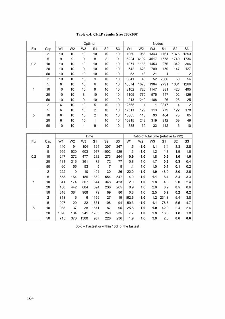
164

Table 6.4: CFLP results (size 200x200)

Optimal Nodes

Fix Cap W1 W2 W3 S1 S2 S3 W1 W2 W3 S1 S2 S3

0.2

2 10 10 10 10 10 10 1960 956 1343 1761 1375 1253

5 9 9 9 8 8 9 6224 4192 4517 1678 1749 1736

10 10 10 10 10 10 10 1071 1166 1453 276 342 306

20 10 10 9 10 10 10 542 623 789 150 147 127

50 10 10 10 10 10 10 53 43 21 1 1 2

1

2 10 10 10 9 10 10 3841 43 52 2066 50 56

5 8 10 10 6 10 10 10574 1673 1904 2791 1031 1266

10 10 10 10 9 10 10 3102 726 1147 881 426 495

20 10 10 8 10 10 10 1105 770 575 147 102 126

50 10 10 9 10 10 10 213 240 188 26 28 25

5

2 6 10 10 5 10 10 12555 1 1 3317 4 2

5 6 10 10 2 10 10 17511 129 113 779 122 178

10 6 10 10 2 10 10 13865 118 93 464 73 65

20 6 10 10 1 10 10 10815 249 319 312 59 49

50 10 10 4 9 10 10 838 69 33 112 6 10

Time Ratio of total time (relative to W2)

Fix Cap W1 W2 W3 S1 S2 S3 W1 W2 W3 S1 S2 S3

0.2

2 140 94 104 324 307 267 1.5 1.0 1.1 3.4 3.3 2.8

5 665 520 603 937 1002 929 1.3 1.0 1.2 1.8 1.9 1.8

10 247 272 477 232 273 264 0.9 1.0 1.8 0.9 1.0 1.0

20 181 216 361 72 72 77 0.8 1.0 1.7 0.3 0.3 0.4

50 60 55 53 5 7 9 1.1 1.0 1.0 0.1 0.1 0.2

1

2 222 10 10 494 30 26 22.0 1.0 1.0 48.9 3.0 2.6

5 653 164 186 1382 554 547 4.0 1.0 1.1 8.4 3.4 3.3

10 341 174 307 844 348 423 2.0 1.0 1.8 4.8 2.0 2.4

20 400 442 884 394 236 265 0.9 1.0 2.0 0.9 0.5 0.6

50 318 384 968 79 69 80 0.8 1.0 2.5 0.2 0.2 0.2

5

2 813 5 6 1159 27 19 162.6 1.0 1.2 231.8 5.4 3.8

5 997 20 22 1551 108 94 50.3 1.0 1.1 78.3 5.5 4.7

10 935 37 38 1571 87 95 25.5 1.0 1.0 42.9 2.4 2.6

20 1026 134 241 1783 240 235 7.7 1.0 1.8 13.3 1.8 1.8

50 715 370 1388 957 228 236 1.9 1.0 3.8 2.6 0.6 0.6

Bold – Fastest or within 10% of the fastest

165

Table 6.4 (continued)

Gap LP (%) Gap XLP (%)

Fix Cap W1 W2 W3 S1 S2 S3 W1 W2 W3 S1 S2 S3

0.2

2 0.5 0.5 0.5 0.2 0.2 0.2 0.10 0.10 0.11 0.11 0.11 0.10

5 9.2 9.2 9.2 0.6 0.6 0.6 0.49 0.50 0.50 0.48 0.49 0.48

10 27.6 27.6 27.6 0.4 0.4 0.4 0.33 0.33 0.34 0.31 0.31 0.31

20 44.9 44.9 44.9 0.4 0.4 0.4 0.29 0.30 0.30 0.22 0.20 0.21

50 58.7 58.7 58.7 0.2 0.2 0.2 0.17 0.15 0.16 0.02 0.01 0.03

1

2 0.1 0.1 0.1 0.1 0.1 0.1 0.05 0.02 0.02 0.05 0.02 0.02

5 1.6 1.6 1.6 0.3 0.3 0.3 0.29 0.24 0.25 0.30 0.25 0.25

10 8.9 8.9 8.9 0.5 0.5 0.5 0.47 0.39 0.39 0.46 0.39 0.40

20 27.6 27.6 27.6 0.4 0.4 0.4 0.40 0.36 0.36 0.39 0.35 0.35

50 53.4 53.4 53.4 0.3 0.3 0.3 0.24 0.23 0.24 0.21 0.20 0.20

5

2 0.1 0.1 0.1 0.1 0.1 0.1 0.10 0.00 0.00 0.09 0.00 0.00

5 0.3 0.3 0.3 0.2 0.2 0.2 0.21 0.07 0.06 0.21 0.07 0.07

10 1.6 1.6 1.6 0.7 0.7 0.7 0.66 0.17 0.16 0.66 0.18 0.18

20 8.1 8.1 8.1 1.8 1.8 1.8 1.74 0.30 0.31 1.73 0.31 0.31

50 31.2 31.2 31.2 1.3 1.3 1.3 1.31 0.20 0.23 1.25 0.18 0.18

Cuts Gap H (%)

Fix Cap W1 W2 W3 S1 S2 S3 W1 W2 W3 S1 S2 S3

0.2

2 92 98 82 31 29 32 0.2 0.1 0.2 0.2 0.2 0.2

5 390 391 381 20 21 21 1.5 0.9 1.1 0.7 0.8 0.7

10 1014 1011 941 15 15 18 1.3 1.1 0.9 0.4 0.4 0.4

20 1536 1532 1280 20 19 20 1.2 1.7 0.9 0.2 0.2 0.2

50 1499 1478 1243 12 12 15 2.3 1.5 0.3 0.0 0.0 0.0

1

2 37 59 52 18 26 23 0.3 0.0 0.0 0.2 0.0 0.0

5 183 239 217 19 21 21 1.0 0.3 0.4 1.1 0.6 0.5

10 572 691 617 11 14 14 1.3 0.9 0.9 0.9 0.5 0.6

20 1848 1871 1482 13 12 11 2.3 3.8 1.8 0.5 0.5 0.6

50 3982 3900 2207 12 12 9 2.5 2.6 1.3 0.2 0.2 0.2

5

2 12 54 47 11 25 20 0.5 0.0 0.0 0.6 0.0 0.0

5 79 166 166 19 20 18 0.9 0.1 0.1 1.3 0.2 0.1

10 191 362 348 12 17 16 2.2 0.5 0.2 2.6 0.2 0.2

20 680 1119 929 9 11 11 3.7 0.8 0.7 4.3 0.7 0.4

50 3972 4298 3099 11 15 18 4.2 1.9 1.5 2.9 0.2 0.2

166

Table 6.5: CFLP results (size 200x200) – summary of time ratios

Ratio of total time Geometric mean of time ratios

S vs. W S1/W1 S2/W2 S vs. W S1/W1 S2/W2

Cap \ Fix 0.2 1 5 0.2 1 5 Cap \ Fix 0.2 1 5 0.2 1 5

2 2.3 2.2 1.4 3.3 3.0 5.4 2 2.8 4.3 4.3 3.0 3.1 5.4

5 1.4 2.1 1.6 1.9 3.4 5.5 5 1.6 3.3 3.1 2.2 3.4 5.2

10 0.9 2.5 1.7 1.0 2.0 2.4 10 1.0 3.0 3.9 1.0 1.9 2.3

20 0.4 1.0 1.7 0.3 0.5 1.8 20 0.4 1.0 2.5 0.3 0.5 1.9

50 0.1 0.2 1.3 0.1 0.2 0.6 50 0.1 0.3 1.3 0.1 0.2 0.6

1 vs. 2 W1/W2 S1/S2 1 vs. 2 W1/W2 S1/S2

Cap \ Fix 0.2 1 5 0.2 1 5 Cap \ Fix 0.2 1 5 0.2 1 5

2 1.5 22.0 162.6 1.1 16.3 43.3 2 1.2 5.9 42.5 1.2 8.2 33.9

5 1.3 4.0 50.3 0.9 2.5 14.3 5 1.3 3.1 25.2 0.9 3.0 14.8

10 0.9 2.0 25.5 0.8 2.4 18.2 10 0.9 1.5 12.1 0.9 2.4 20.6

20 0.8 0.9 7.7 1.0 1.7 7.4 20 0.8 0.9 5.8 1.0 1.8 7.8

50 1.1 0.8 1.9 0.7 1.1 4.2 50 1.0 0.8 2.0 0.8 1.1 4.2

Combined S1/W2 Combined S1/W2

Cap \ Fix 0.2 1 5 Cap \ Fix 0.2 1 5

2 3.4 48.9 231.8 2 3.5 25.7 182.5

5 1.8 8.4 78.3 5 2.1 10.2 77.0

10 0.9 4.8 42.9 10 0.9 4.5 47.2

20 0.3 0.9 13.3 20 0.3 0.9 14.6

50 0.1 0.2 2.6 50 0.1 0.2 2.6

Table 6.6: CFLP instances – average number of violated variable upper bound constraints (B) by

the first LP relaxation of the weak formulation, relatively to the number of centers (n)

Cap \ Fix 0.2 1 5

2 25% 6% 2%

5 96% 69% 23%

10 100% 100% 73%

20 100% 100% 100%

50 100% 100% 100%

167

6.2.7 CFLPSS results

CFLPSS results are presented in Table 6.7 and Table 6.8. We first note that instances

are harder to solve for lower capacity ratios and higher fixed costs, similarly to what

was observed for the CFLP (however, for the CFLPSS this applies also to aggregate

formulations with low capacity levels, which was not the case for the CFLP). For the

instances tested, the CFLPSS becomes much easier to solve for capacity level 5 or

higher. The explanation is that, with larger facility capacities, more centers satisfy

single sourcing constraints even if these are omitted (solving a CFLP with the same

instances we observed that the proportion of centers assigned to more than one facility

in optimal solutions were 27%, 17%, 10% and 5% for capacity levels of 2, 3, 4 and 5,

respectively, in the case of fixed cost level 1).

We find, like for the CFLP, that aggregate formulations are generally solved faster than

the standard ones (except with fixed cost level 0.2, for which instances are relatively

easy and standard formulations are slightly faster) and weak formulations are generally

solved faster than the corresponding strong ones. Comparing aggregate formulations 3

and 2, the best one varies for different data, both for the strong and weak variants.

In Table 6.8 we summarize the relative performance of formulations (we omit Cap=5,

as instances are easily solved in under 20 seconds on average with aggregate

formulations; we consider formulation 3 instead of 2 like for the CFLP, since S3 is

solved about twice as fast as S2 for the harder instances with Cap=2 and Fix=1 and 5).

Weak formulations are solved faster than strong ones by a factor of up to about 1.5 for

Fix=1. Aggregate formulations 3 are solved faster than the standard ones by a factor of

about 1.5-3 times for Fix=1. The last panel (S1/W3) shows that if one adopts the

standard strong formulation (S1) rather than the more effective W3, solution times can

be higher by a factor of 4 or more for Fix=1 or 5.

Unlike for the CFLP, the relative performance of formulations for individual instances

(tables show only aggregate results) is not systematic, i.e. one formulation with higher

average time may be solved faster in particular instances. For this reason, in Table 6.8

the ratio of total time may be less than 1 but the geometric mean of time ratios may be

higher than 1 (or vice versa).

In conclusion, on the basis of our experiments, the W2 or W3 formulations are

recommended for the CFLPSS for capacity levels of up to 5 (and possibly higher).

Although we did not test much higher capacity levels (say of more than 10), the

168

CFLPSS can be expected to reduce to the CFLP and formulations S2 or S3 are likely to

perform better, as for the CFLP.

Table 6.7: CFLPSS results (size 50x50)

Optimal Nodes

Fix Cap W1 W2 W3 S1 S2 S3 W1 W2 W3 S1 S2 S3

0.2

2 10 10 10 10 10 10 3664 3503 5118 5564 5135 7613

3 10 10 10 10 10 10 1139 1527 1262 1146 1303 1140

5 10 10 10 10 10 10 371 355 538 378 162 361

1

2 7 9 10 6 9 9 25963 20174 11181 22482 18420 12294

3 9 10 10 10 10 10 98336 7788 8395 15889 9185 8600

5 10 10 10 10 10 10 2641 1255 1224 3462 1231 1152

5

2 8 9 9 5 8 10 30249 16633 104725 50250 20939 9224

3 10 10 10 7 10 10 74783 25966 11038 162461 16857 15548

5 10 10 10 10 10 10 16449 3056 1440 24674 2551 2188

Time Ratio of total time (relative to W2)

Fix Cap W1 W2 W3 S1 S2 S3 W1 W2 W3 S1 S2 S3

0.2

2 80 76 88 111 151 128 1.1 1.0 1.2 1.5 2.0 1.7

3 18 28 25 23 28 25 0.6 1.0 0.9 0.8 1.0 0.9

5 5 6 9 8 7 8 0.8 1.0 1.5 1.3 1.1 1.3

1

2 751 362 257 1025 610 357 2.1 1.0 0.7 2.8 1.7 1.0

3 284 69 89 211 121 129 4.1 1.0 1.3 3.1 1.8 1.9

5 18 12 16 29 14 13 1.5 1.0 1.3 2.4 1.2 1.1

5

2 852 364 473 1235 630 284 2.3 1.0 1.3 3.4 1.7 0.8

3 289 164 93 915 170 240 1.8 1.0 0.6 5.6 1.0 1.5

5 31 11 9 86 16 18 2.8 1.0 0.8 7.7 1.4 1.6

Bold – Fastest or within 10% of the fastest

Gap LP (%) Gap XLP (%)

Fix Cap W1 W2 W3 S1 S2 S3 W1 W2 W3 S1 S2 S3

0.2

2 6.0 6.0 6.1 5.0 5.0 5.1 0.58 0.56 0.51 0.57 0.56 0.61

3 7.5 7.5 7.5 3.6 3.6 3.6 0.75 0.78 0.83 0.70 0.70 0.78

5 16.0 16.0 16.0 2.7 2.7 2.7 0.81 0.80 0.87 0.76 0.71 0.86

1

2 2.1 2.1 2.1 2.1 2.1 2.1 0.66 0.27 0.25 0.66 0.27 0.25

3 2.4 2.4 2.4 1.8 1.8 1.8 0.82 0.55 0.55 0.82 0.54 0.54

5 5.5 5.5 5.5 2.2 2.2 2.2 1.56 1.11 1.08 1.52 1.08 1.09

5

2 1.1 1.1 1.1 1.1 1.1 1.1 0.68 0.06 0.06 0.70 0.06 0.05

3 1.1 1.1 1.1 1.0 1.0 1.0 0.82 0.09 0.08 0.77 0.10 0.09

5 1.9 1.9 1.9 1.7 1.7 1.7 1.52 0.19 0.19 1.41 0.18 0.19

169

Table 6.7 (continued)

Cuts Gap H (%)

Fix Cap W1 W2 W3 S1 S2 S3 W1 W2 W3 S1 S2 S3

0.2

2 182 235 148 249 166 148 3.7 2.5 2.8 1.9 2.3 5.3

3 127 143 152 93 95 91 2.6 3.2 3.6 1.9 2.6 2.6

5 150 153 169 52 52 46 1.7 2.1 3.2 2.5 1.0 3.6

1

2 147 225 216 168 206 188 4.1 5.2 7.3 3.9 5.0 8.2

3 136 184 130 92 93 91 4.0 6.2 8.2 4.0 5.8 8.6

5 97 140 152 36 32 38 4.9 6.3 8.0 5.0 6.1 7.4

5

2 172 236 238 176 190 192 4.4 5.2 7.6 5.1 4.9 7.5

3 81 114 222 63 90 109 4.2 4.8 8.2 4.3 5.7 8.8

5 58 119 104 27 36 37 5.7 4.5 6.0 4.2 4.1 3.5

Table 6.8: CFLPSS results (size 50x50) – summary of time ratios

Ratio of total time Geometric mean of time ratios

S vs. W S1/W1 S3/W3 S vs. W S1/W1 S3/W3

Cap \ Fix 0.2 1 5 0.2 1 5 Cap \ Fix 0.2 1 5 0.2 1 5

2 1.4 1.4 1.4 1.5 1.4 0.6 2 1.2 1.6 1.8 1.6 1.1 1.0

3 1.3 0.7 3.2 1.0 1.4 2.6 3 1.2 1.2 2.8 1.2 1.4 2.5

1 vs. 3 W1/W3 S1/S3 1 vs. 3 W1/W3 S1/S3

Cap \ Fix 0.2 1 5 0.2 1 5 Cap \ Fix 0.2 1 5 0.2 1 5

2 0.9 2.9 1.8 0.9 2.9 4.3 2 1.1 2.7 2.9 0.9 4.0 5.3

3 0.7 3.2 3.1 0.9 1.6 3.8 3 0.8 1.5 2.3 0.8 1.3 2.6

Combined S1/W3 Combined S1/W3

Cap \ Fix 0.2 1 5 Cap \ Fix 0.2 1 5

2 1.3 4.0 2.6 2 1.4 4.4 5.2

3 0.9 2.4 9.8 3 0.9 1.8 6.4

170

6.3 Capacitated median model

6.3.1 Formulations

In the capacitated median (CM) model the aim is to locate facilities and assign all

demand centers to those facilities so that the total travel distance (or time) is minimized,

centers are assigned to the closest facility, and facilities satisfy minimum and maximum

capacity bounds.

Fixed costs are not considered in this model but, like in the previous models, the

number of facilities is a model output, resulting from the upper and lower bounds

imposed by the minimum and maximum capacity constraints, respectively. The model

is called the capacitated median model due to its relation with the classic p-median

model – see the discussion by Teixeira and Antunes (2008), who also review

applications, mostly dedicated to the location of health care and education facilities.

Here we consider a restricted version of this model with non-binding maximum

capacity bounds, thus no maximum capacity constraints are included, and with constant

minimum capacity bounds. We consider the same notation as in the previous models

and additionally: jb b is the minimum facility capacity for site j J ; tij is the travel

distance (or time) between center i I and site j J ; ij ij ic t d for i I , j J .

The strong formulation of the CM model is as follows:

(S1-CM):

Min ij iji I j J

c x

Subject to 1ijj J

x

, i I (D)

ij jx y , ,i I j J (B)

i ij j ji I

d x b y

, j J (C)

: ik ij

ij jk J t t

x y

, ,i I j J (CA)

{0,1}jy , j J (I)

{0,1}ijx , ,i I j J (SS)

where (C) are minimum capacity constraints and (CA) are closest assignment

constraints, stating that if a facility is installed at j, then center i has to be assigned to a

facility at a travel distance of tij or less.

171

The weak formulation of the CM model, (W1-CM), is obtained from (S1-CM) by

replacing (B) with (U).

If the CM model is augmented with maximum capacity constraints (C), the aggregate

constraints with redundant information discussed for the CFLP can also be added. We

now discuss analogous constraints for the case of minimum capacities. The constraint

analogous to (T) is

j j ij J i I

b y d

. (T)

Since jb b for j J is assumed, this constraint can be reduced to

j ii Ij J

y d b

(T )

which now is not redundant for the LP formulation since the integer round-down

function was applied. The constraints analogous to (C ) are

j j jz b y , j J (C )

Let (S2-CM) denote (S1-CM) with (T ) added.

Let (S3-CM) denote (S2-CM) with (C) replaced by (C ) and (Z), (F), (Nz) added.

Let (W2-CM) and (W3-CM) denote, respectively, (S2-CM) and (S3-CM) with (B)

replaced by (U).

Note: Van Roy and Wolsey (1986) first introduced a variant of flow cover inequalities

considering lower capacity bounds as well as upper bounds, which would apply to the

single node flow structure in formulations S3 and W3 above. Even though Xpress can

generate flow cover cuts, the documentation does not make clear if they include the

variant for lower capacity bounds.

6.3.2 Instances

Test instances for the CM model were randomly generated and assumed identical sets of

centers and sites (I = J). First, for a given size n (number of centers), 9 data sets (cij, ui)

were created: points representing centers were uniformly generated in [0,100][0,100];

ui = 1000/nUniform[0.1,1.9]; cij = uidij, where dij is the Euclidean distance between

centers i and j. Then, the capacity ratio r, equal to total demand divided by the minimum

capacity (i.e. the expected maximum number of open facilities), was used as a control

parameter to derive 4 instances from each data set (cij, ui) by setting ii Ib u r for

172

r = n0.1, 0.2, 0.3, and 0.4. All data was rounded to integer values. Here we consider

instances of a single size n = 70.

6.3.3 Software

The same MIP optimizer and computer were used as in the other models. All solver

parameters were left at default values, except that branching priority was given to y

variables. All instances were solved to optimality (in less than 30 minutes).

6.3.4 Results

Regarding weak formulations for the CM model, W2 was tested first and was verified

not to be competitive with S2. Thus other weak formulations were not tested.

Results are shown in Table 6.9 and the following can be observed:

S2 can be considered better than S1 and W2 as it is solved significantly faster

for one or both of the harder, smaller capacity ratios r=7 and 14, while being

similar or not much worse for other ratios r.

S3 has an overall performance similar to S2 and no formulation seems to

dominate the other.

Based on these results, we conclude that it is indifferent to choose either S2 or S3, and

both are preferable to S1 and W2.

We also observe that the solver closes the XLP gaps of W2 to values similar to those of

S2. Some surprising XLP gaps are observed (but were not further analyzed): the XLP

gap of W2 is the smallest among all formulations for r=7; the XLP gap of S1 is smaller

than the one of S2 for r=14 and 28.

173

Table 6.9: CM model results (size 70x70)

n-r Optimal Nodes

S1 S2 S3 W2 S1 S2 S3 W2

70-7 9 9 9 9 2509 1743 1259 2154

70-14 9 9 9 9 1055 1273 1451 1824

70-21 9 9 9 9 96 83 83 136

70-28 9 9 9 9 4 4 3 6

70 total 36 36 36 36 916 776 699 1030

n-r Time Ratio of total time

S1 S2 S3 W2 S1 S2 S3 W2

70-7 652 368 325 724 1.8 1.0 0.9 2.0

70-14 283 331 355 422 0.9 1.0 1.1 1.3

70-21 50 55 64 49 0.9 1.0 1.2 0.9

70-28 35 35 28 29 1.0 1.0 0.8 0.8

70 total 255 197 193 306 1.3 1.0 1.0 1.6

n-r Gap LP (%) Gap XLP (%)

S1 S2 S3 W2 S1 S2 S3 W2

70-7 8.3 5.6 5.6 49.1 6.3 4.0 4.2 3.8

70-14 10.7 9.9 9.9 30.8 3.2 3.4 3.8 3.3

70-21 13.9 13.6 13.8 23.1 1.0 1.0 0.7 1.0

70-28 15.3 15.3 21.1 26.6 0.2 0.4 0.2 0.4

70 total 12.1 11.1 12.6 32.4 2.7 2.2 2.2 2.1

n-r Cuts Gap H (%)

S1 S2 S3 W2 S1 S2 S3 W2

70-7 108 91 61 529 12.7 9.1 6.4 7.9

70-14 198 195 188 365 6.9 9.5 7.3 9.2

70-21 133 121 147 205 1.3 1.3 3.1 1.2

70-28 117 116 63 112 0.3 1.0 0.3 0.5

70 total 139 131 115 303 5.3 5.2 4.3 4.7

174

6.4 Conclusion

We presented an empirical investigation of solving the CFLP with a generic MIP

optimizer, comparing several formulation variants. Test instances, generated with a

procedure often used for benchmarking purposes, cover a wide range of capacity levels

(total potential capacity divided by total demand) and fixed cost levels, since solution

times and the relative performance of formulations strongly depend on these parameters.

Our results show that the CFLP can be solved faster with a generic MIP optimizer by

considering: (i) a formulation with additional constraints to help the solver detect

certain model relaxations, which may not be recognized automatically and for which

strong cutting planes can be generated; (ii) the weak variant of the formulation instead

of the strong one, for lower capacity levels (up to 10 in our tests and for a wide range of

fixed cost levels).

The first recommendation follows the one by Aardal (1998b), who reported significant

solution time reductions with the research-oriented MINTO optimizer. Here we confirm

the same applies to a modern commercial optimizer, with time being reduced by a factor

of 2-10 or more, depending on the capacity level.

Using the weak variant of the formulation reduces time further by a factor of 2 or more.

Time reductions increase for higher fixed cost levels and lower capacity levels. The

good performance of weak relative to strong formulations can be attributed to the fact

that fewer variable upper bound constraints are required to strengthen the LP relaxation

when capacities are tighter, and to faster re-optimization of the smaller formulations at

branch-and-bound nodes (even though more nodes may be explored). For higher

capacity levels, as the CFLP tends to reduce to the UFLP, the strong formulation

becomes more effective, since variable upper bound constraints are essential to tighten

LP bounds.

For the CFLPSS similar results were obtained, although with lower time reductions. For

the capacitated median model, an unrelated model, similar results were not obtained and

the strong formulation was more effective.

The results of our experiments can be useful for practitioners wishing to solve the CFLP

or CFLPSS model with a generic MIP optimizer, with minimal effort without resorting

to a specialized algorithm. They can also be useful for obtaining a benchmark for

comparing with a specialized algorithm, by using the most effective formulation

available in a generic MIP optimizer.

175

In out experiments we used the Xpress optimizer. We expect that similar results are

likely to be obtained with other software, such as CPLEX or Gurobi, but this was not

tested.

With the particular version of Xpress used, we verified that performance increased (for

all formulations of all models) by changing default cut generation parameters to a less

conservative one (in terms of the number of cuts the solver is allowed to add). However,

we did not aim to optimize solver parameters for the location models tested (e.g. by

switching off the generation of ineffective cut types or by tuning tree search strategies),

and the conclusions above implicitly assume such optimization, if possible, would not

change the relative performance of formulations significantly.

177

Chapter 7

Conclusion

7.1 Discussion of applications

Model applications in chapters 2, 3 and 4 were presented independently. This section

offers a comparison of these applications, in order to further clarify the modeling

assumptions adopted, and to further discuss the adequacy and limitations of the models.

Model assumptions

Inelastic demand: Both the school and court location applications assumed exogenous

and inelastic demand with respect to travel costs (any other user-supported costs are

assumed not to vary by location and to be already reflected in the demand forecasts). In

the case of schools, this assumption is reasonable since primary and secondary

education are mandatory (however, for extra-curricular education activities, such as

music or sports, demand is likely to be elastic and the models used would not be

representative). In the case of justice, it was deemed reasonable to assume most

litigation demand is inelastic with respect to travel costs.

Minimum capacity: In applications to schools, minimum capacity bounds were set

according to the guidelines on school size by the Ministry of Education, in the case of

new schools, and were set for the purposes of the study in agreement with the Municipal

Council of Coimbra, in the case of existing schools. These bounds reflect concerns both

with student achievement in too small schools and with financial sustainability. In the

application to courts, minimum capacity bounds were set for the purposes of the study

in agreement with the Ministry of Justice and reflect concerns with financial

sustainability, as well as with guaranteeing diversity of experience for judges in

specialized courts.

Closest assignment: In all applications, assignment of demand centers to the closest

facility was a planning assumption. In the case of courts, this assumption can be

considered appropriate, since assignment to courts is mandated by the responsible

public authority, taking into account proximity to the defendant’s location. In this

178

context, assuming closest assignment is likely to increase public confidence and

acceptance of solutions.

In the case of schools, the appropriateness of the closest assignment assumption can be

debated, since school assignment is not strictly mandated in Portugal: when applying

their children to a new school, parents can specify a preference ordering of up to 5

schools (until 2011 primary schools had to be chosen within the home or work area of

one of the parents; since 2012 any school can be chosen).

On the one hand, it is observed that proximity to home is, by far, the most important

factor parents take into account when choosing a school for their children, as already

stated in chapter 2. According to a survey carried out for Coimbra’s Educational Charter

(Canavarro et al., 2004), the two most frequent factors identified by parents were

proximity to home (63% of respondents) and teacher quality (38%); proximity to

workplace was much less frequent (18%). In addition, when the number of applicants

for a school exceeds its capacity, proximity to home is by law one of the primary factors

school directors take into account for approving applications. On the other hand, it

should be acknowledged that proximity to home is not the only or the most important

preference factor for all people.

To further discuss this issue, we outline two alternative approaches for a school network

planning problem, differing in the treatment of user preferences (the two approaches

were also discussed and exemplified in the literature review of chapter 2):

(1) Assume that accessibility is the main factor in school choice, and use a model that

maximizes accessibility and assumes closest assignment. This was the approach

followed in this thesis, with accessibility being defined in relation to the place of

residence.

(2) Assume that preferences for schools include accessibility and other factors such as

perceived teaching quality, and use a model that maximizes the preferences met. This

approach requires describing and measuring the attractiveness of facilities and the

preferences of users, and weighting preferences into a single measure.

It can be argued that the first approach is more appropriate for strategic planning

problems that focus on defining the location and capacity of facilities in the long-term

(e.g. in a horizon of 10 years). User preferences are considered only approximately by

focusing on accessibility. The closest assignment assumption is also compatible with

stated principles of education and spatial planning policies, of providing high education

quality across all schools (according to the Basic Law of the Education System in

179

Portugal) and of providing education services in proximity to residential areas (as stated

in Coimbra’s Educational Charter).

In contrast, the second approach is more appropriate for operational problems of

managing installed capacity in the short-term (e.g. on a yearly basis) that focus on

defining assignments of users to facilities once user preferences are declared. If such an

approach is used for a strategic planning problem, it requires forecasting the

attractiveness of facilities and the preferences of users into the future (including in

relation to potential new facilities), with results that are likely to be very inaccurate and

to generate controversy among decision makers.

To conclude, assuming that closest assignment applies to all users is debatable in the

case of schools. This was a planning assumption deemed reasonable in the applications

in this thesis, but it may not be suitable for all school planning applications, e.g. if

schools are expected in the future to have widely varying perceived education quality

and parents can freely choose schools regardless of proximity to home.

Data preparation

Aggregation of population centers: In chapter 2 (secondary schools), the municipality of

Coimbra was discretized into 43 population centers, while in chapter 3 (primary

schools) the same region was discretized into 68 centers. The more detailed

discretization is justified by the fact that proximity is a greater concern for primary

schools, particularly for the first level schools (EB1), which exist in a larger number and

have smaller catchment areas.

Travel distances or times: In all applications, travel distances or times were computed

using a representation of the main road network. In the applications to schools, travel

distances were used, which assumes that a constant average travel speed is

representative of both private and public transportation under average congestion levels.

This was considered acceptable since the spatial context is a municipality with moderate

congestion levels and served by an extensive bus network. In the application to courts,

travel times were used. Since the spatial context is a larger region, different average

speeds were considered according to the hierarchical level of roads.

Model ingredients

Single vs. multiple services: in both secondary and primary school applications,

education demand comprises two education levels. For secondary schools (chapter 2), a

single service model is used, with demand for a single service representing two

180

education levels (S1 and S2), being offered at a single facility type (ES12 schools). This

could be assumed because both education levels should be assigned to the same school,

and school capacity is shared by the two levels. For primary schools (chapter 3), a two-

level service model is used, since two facility types are to be located – EB1 schools for

B1 education and EB12 schools for both B1 and B2 education.

Co-location of existing and new facilities: In the secondary school model (chapter 2),

the formulation allows the co-location of up to one existing facility and one new

facility. This choice is justified because the spatial aggregation level is high and in some

central population centers existing capacity is tight.

In the primary school model (chapter 3) the formulation allows the co-location of level-

1 and level-2 facilities but not of new and existing facilities of the same type. In this

application, the spatial aggregation level is smaller, but still level-1 and level-2 facilities

exist in very close proximity in some centers. On the other hand, the existing capacity of

level-2 facilities is generally not tight.

Path assignment: Path assignment (PA) constraints are introduced in chapter 3, where it

is stated that they are an alternative to closest assignment (CA) constraints. Here we

make two observations. First, in a model with PA replacing CA constraints, assignments

may no longer be compatible with free choices of users that aim to minimize their

individual travel costs. Thus, such model assumes that the public authority has the

power to mandate assignments. In this context, PA constraints help by producing a

spatial configuration of assignments that may be more easily accepted by users.

Second, PA and CA constraints may be used in combination if CA constraints are

retained in the model but their data is modified so that they now forbid assignments

further than a given tolerance relatively to the closest facility. As an example of such

tolerance, model solutions in chapter 3 (primary schools) would remain the same if CA

constraints were retained but given an absolute tolerance of 2.5 km.

Coherent assignment: This type of constraints was used in the application to courts

(chapter 4), but not in the application to primary schools (chapter 3), where a two-level

nested hierarchical model is also used. In the latter, the problem statement did not

require coherent assignment constraints. However, if required, such constraints could be

added to the model.

Hierarchical models: The applications to primary schools (chapter 3) and to courts

(chapter 4) both consider models with a two-level nested hierarchy of facilities: low-

level facilities serving only level-1 demand, and high-level facilities serving both level-

181

1 and level-2 demand. However, the formulation of the nested hierarchy is different in

the two models, reflecting differences in problem statements. In the primary school

location model, a level-2 facility corresponds to a single school that serves the two

demand levels and capacity is shared by the two levels; the nested hierarchy is enforced

by constraints (3.19) linking assignment and location variables. In the court location

model, level-1 and level-2 facilities may be physically distinct, each one serves only the

corresponding demand level and is subject to independent capacity constraints; the

nested hierarchy is enforced by constraints (4.18) linking location variables.

7.2 Overall conclusion and contributions

An overall conclusion of the thesis is now presented, complementing the individual

conclusions of previous chapters.

The discrete facility location models studied in this thesis provided a useful contribution

to real-world public facility planning problems of reorganizing networks of schools and

courts of justice. While the basic, single-service model had been previously presented in

the literature, multiple-service (hierarchical) variants had not been presented before,

combining hierarchical facilities, minimum capacity constraints and different types of

constraints on the spatial pattern of user-to-facility assignments: closest assignment,

path assignment, and coherent assignment.

Regarding solution methods, modern generic MIP optimization software proved to be

robust and efficient to deal with the public facility planning applications in this thesis.

Model instances in these applications turned out to be relatively easy to solve, since

significant constraints were imposed on planning decisions in the context of

reorganizing existing facility networks, such as limiting the numbers of new facilities to

open and of existing facilities to close, or restricting assignments to existing

administrative boundaries, thereby reducing the number of free decision variables.

The performance of generic MIP optimizers has been improving remarkably, as

discussed in the references cited in section 1.3 and as illustrated by the results reported

with Xpress versions 2005B and 7.2 in chapter 5. Nevertheless, a careful choice of

model formulation is still recommended in order to take full advantage of modern MIP

optimizers. For example, the alternative formulations of closest assignment constraints

tested in chapter 5 (second appendix) lead to widely varying solution times. For the

CFLP model, adding constraints with redundant information to help cut generation

(following advice from the literature), and using the so-called weak formulation if

capacity data is tight, can significantly reduce solution times, as tested in chapter 6.

182

The specialized solution method developed in chapter 5 for the single-service

capacitated median model reduces the solution time of relatively large instances with

100 centers by 20-50% (with Xpress 7.2) relatively to the standard formulation. This

reduction is mainly due to the a priori reformulation procedure adapted from previous

work. Some new valid inequalities were presented, but they turned out not to be

effective at further reducing solution times when used to generate cuts in a branch-and-

cut algorithm.

Regarding the objectives outlined in the introduction, it can be said that they were

generally accomplished, with some exceptions related to the development of specialized

solution methods. First, for the single service model, the original work developed in this

thesis gave only a modest improvement in solution times, as mentioned above. Second,

while the development of specialized methods for multiple service models was an

objective of the thesis, this work was not carried out and is left for future work.

The contributions of this thesis to the discrete facility location literature are the

following:

Formulation of optimization models combining multiple services, minimum and

maximum capacity constraints, and constraints on the spatial pattern of

assignments of users to facilities, extending previous hierarchical facility

location models;

Description of applications of models with single and multiple services to real-

world problems of reorganizing networks of schools and courts of justice in

Portugal;

Development of new valid inequalities for the MIP formulation of the single

service capacitated median model and proposal of an exact solution method,

composed of a priori reformulation and branch-and-cut, that reduces solution

times relatively to a generic MIP optimizer;

Presentation of computational experiments on solving single service models

with a modern generic MIP optimizer, including the fixed-charge capacitated

facility location problem and the capacitated median model, in order to identify

the most efficient formulation, among variants known from the literature, to

solve these models to optimality without resorting to a specialized algorithm.

183

7.3 Future work

Possible future work arising from the work in this thesis can be outlined as follows:

Adapt the reformulation procedure and specialized cuts of chapter 5 to the

hierarchical models. Such an adaption should be relatively straightforward, since

the valid inequalities can be applied to each service level separately. However its

effectiveness to reduce solution times remains to be tested.

Develop other separation procedures for the new valid inequalities proposed in

chapter 5, to better exploit them in a branch-and-cut algorithm.

Study the single and multiple-service models under uncertainty in the model

data. Uncertainty in demand, rather than in travel costs, is deemed the most

relevant for the types of applications studied in this thesis. The deterministic

model can be used to solve independently a limited number of scenarios of data

realizations (say, pessimistic, reference and optimistic scenarios of demand), but

in this case comparing the solutions and selecting a final solution are left outside

the scope of the model. In order to model uncertainty, and obtain a solution that

“performs well” under all possible data realizations, a possible approach is

scenario planning (Owen and Daskin, 1998; Current et al., 2002).

Study alternative formulations of the hierarchical model with coherency

constraints (the second model in chapter 4). A large number of coherency

constraints is required (number of centers cubed) with the adopted formulation

and its strength was not analyzed in this thesis (nor in previous work, as far as

we know). Computational experiments with larger instances than those of the

practical application in chapter 4 were also not performed. If such instances turn

out to be hard to solve, an improved formulation would be useful.

185

References

Aardal, K. (1998a). Capacitated facility location: separation algorithms and compu-

tational experience. Mathematical Programming, 81 (2), 149-175.

Aardal, K. (1998b). Reformulation of capacitated facility location problems: how

redundant information can help. Annals of Operations Research, 82 (0), 289-308.

Ahuja, R. K., Orlin, J. B., Pallottino, S., Scaparra, M. P., & Scutella, M. G. (2004). A

multi-exchange heuristic for the single source capacitated facility location.

Management Science, 50 (6), 749-760.

Antunes, A. (1994). De la Planification Optimale de l'Équipement Scolaire [Optimal

planning of school infrastructure]. PhD thesis, Catholic University of Louvain,

Belgium.

Antunes, A., & Peeters, D. (2001). On solving complex multi-period location models

using simulated annealing. European Journal of Operational Research, 130 (1), 190-

201.

Ashford, R. (2007), Mixed integer programming: a historical perspective with Xpress-

MP. Annals of Operations Research, 149 (1), 5-17.

Atamturk, A., & Savelsbergh, M. W. P. (2005). Integer programming software systems.

Annals of Operations Research, 140 (1), 67-124.

Avella, P., & Boccia, M. (2009). A cutting plane algorithm for capacitated facility

location problems. Computational Optimization and Applications, 43 (1), 39-65.

Avella, P., Boccia, M., & Salerno, S. (2011). A computational study of dicut

reformulation for the single source capacitated facility location problem. Studia

Informatica Universalis, 9 (3), 21-42.

Balakrishnan, A., Magnanti, T. L., & Wong, R. T. (1995). A decomposition algorithm

for local access telecommunications network expansion planning. Operations

Research, 43 (1), 58-76.

Barahona, F., & Chudak, F. (2005). Near optimal solutions to large scale facility

location problems. Discrete Optimization, 2 (1), 35-50.

Belotti, P., Labbé, M., Maffioli, F., & Ndiaye, M. M. (2007). A branch-and-cut method

for the obnoxious p-median problem. 4OR, 5 (4), 299-314.

186

Berman, O., Drezner, Z., Tamir, A., & Wesolowsky, G. (2009). Optimal location with

equitable loads. Annals of Operations Research, 167 (1), 307-325.

Berman, O., Krass, D., & Wang, J. (2006). Locating service facilities to reduce lost

demand. IIE Transactions, 38 (11), 933-946.

Bigotte, J. F., & Antunes, A. P. (2007). Social infrastructure planning: a location model

and solution methods. Computer-Aided Civil and Infrastructure Engineering, 22 (8),

570-583.

Bixby, R. (2011). The Gurobi optimizer. Presentation slides, Integer Programming

Down Under (IPDU) workshop, University of Newcastle, Australia. Retrieved from

http://carma.newcastle.edu.au/ nuor/ipdu/abstracts.html

Bixby, R., & Rothberg, E. (2007). Progress in computational mixed integer

programming – a look back from the other side of the tipping point. Annals of

Operations Research, 149 (1), 37-41.

Bixby, R., Fenelon, M., Gu, Z., Rothberg, E., & Wunderling, R. (2000). MIP: theory

and practice – closing the gap. In Powell, M. J. D., & Scholtes, S. (Eds.), System

modeling and optimization: methods, theory and applications (pp. 19-49). Kluwer.

Blum, C., & Roli, A. (2003), Metaheuristics in combinatorial optimization: overview

and conceptual comparison. ACM Computing Surveys, 35(3), 268-308.

Brakman, S., Garretsen, H., & Van Marrewijk, C. (2001). An introduction to

geographical economics. Cambridge University Press.

Canavarro, J. M., Pereira, M. D., David, R. M., Ramos, L. M., & Silva, P. (2004).

Avaliação das expectativas da população sobre as escolas [Evaluation of the

expectations of the population about schools]. Relatório para a Carta Educativa de

Coimbra, Faculdade de Psicologia e Ciências da Educação, Universidade de

Coimbra, Portugal.

Cánovas, L., García, S., Labbé, M., & Marín, A. (2007). A strengthened formulation for

the simple plant location problem with order. Operations Research Letters, 35 (2),

141-150.

Caro, F., Shirabe, T., Guignard, M., & Weintraub, A. (2004). School redistricting:

embedding GIS tools with integer programming. Journal of the Operational

Research Society, 55 (8), 836-849.

187

Carreras, M., & Serra, D. (1999). On optimal location with threshold requirements.

Socio-economic Planning Sciences, 33 (2), 91-103.

Chadwick, G. (1978). A systems view of planning. Pergamon Press.

Church, R. L., & Murray, T. (1993). Modeling school utilization and consolidation,

Journal of Urban Planning and Development, 119 (1), 23-38.

Church, R. L. (2002). Geographical information systems and location science.

Computers & Operations Research, 29 (6), 541-562.

Church, R. L. (2003). COBRA: a new formulation of the classic p-median location

problem. Annals of Operations Research, 122 (1-4), 103-120.

Church, R. L., & Eaton, D. J. (1987). Hierarchical location analysis using covering

objectives. In Ghosh, A., & Rushton, G. (Eds.), Spatial analysis and location-

allocation models (pp. 163-185). Van Nostrand Reinhold.

Church, R. L., & Murray, A. T. (1993). Modeling school utilization and consolidation.

Journal of Urban Planning and Development, 119 (1), 23-38.

Church, R. L., & Schoepfle, O. B. (1993). The choice alternative to school assignment.

Environment and Planning B, 20 (4), 447-457.

Cordeau , J.-F., Pasin, F., & Solomon, M. M. (2006). An integrated model for logistics

network design. Annals of Operations Research, 144 (1), 59-82.

Cornuejols, G., Nemhauser, G. L., & Wolsey, L. A. (1990). The uncapacitated facility

location problem. In Mirchandani, P.B., & Francis, R.L. (Eds.), Discrete location

theory (pp. 119-171). Wiley.

Cornuejols, G., Sridharan, R., & Thizy, J. M. (1991). A comparison of heuristics and

relaxations for the capacitated facility location problem. European Journal of

Operational Research, 50 (3), 280-297.

Csirik, J., Johnson, D. S., & Kenyon, C. (2001). Better approximation algorithms for bin

covering. Proceedings of the 12th Annual ACM-SIAM Symposium on Discrete

Algorithms, 557-566.

Current, J., Daskin, M. S., & Schilling, D. (2002). Discrete network location models. In

Drezner, Z., & Hamacher, H. (Eds), Facility location: applications and theory (pp.

81-118). Springer.

188

Dash Optimization, Ltd (2002). Xpress-Optimizer reference guide – release 14.

Blisworth, UK.

Dash Optimization, Ltd (2004), Xpress-Mosel language reference manual – release 1.4.

Blisworth, UK.

Dash Optimization, Ltd (2005), Xpress-Optimizer reference manual – release 15.

Blisworth, UK.

Daskin, M. S. (1995). Network and discrete location: models, algorithms, and

applications. Wiley.

Deng, Q., & Simchi-Levi, D. (1992). Valid inequalities, facets and computational

results for the capacitated concentrator location problem. Working paper,

Department of Industrial Engineering and Operations Research, Columbia

University, New York.

Densham, P. J., & Rushton, G. (1996). Providing spatial decision support for rural

public service facilities that require a minimum workload. Environment and

Planning B, 23 (5), 553-574.

DGS – Direcção-Geral da Saúde (2001). Rede de referenciação hospitalar de

intervenção cardiológica [Hospital referral network of interventional cardiology].

Ministério da Saúde, Lisboa, Portugal.

Díaz, J. A., & Fernández, E. (2002). A branch-and-price algorithm for the single source

capacitated plant location problem. Journal of the Operational Research Society, 53

(7), 728-740.

Draper, N. R., & Smith, H. (1998). Applied regression analysis (3rd ed.). Wiley.

Duque, J. C., Church, R. L., & Middleton, R. S. (2011). The p-regions problem.

Geographical Analysis, 43 (1), 104-126.

Eiselt, H. A., & Laporte, G. (1995). Objectives in location problems. In: Drezner, Z.

(Ed.), Facility location: a survey of application and methods (pp. 151-180).

Springer.

Eitan, Y., Narula, S. C., & Tien, J. M. (1991). A generalized approach to modeling the

hierarchical location-allocation problem. IEEE Transactions on Systems, Man, and

Cybernetics, 21 (1), 39-46.

189

Erlenkotter, D. (1978). A dual-based procedure for uncapacitated facility location.

Operations Research, 26 (6), 992-1009.

Espejo, I., Marín, A., & Rodríguez-Chía, A. M. (2012). Closest assignment constraints

in discrete location problems. European Journal of Operational Research, 219 (1),

49-58.

ESRI – Environmental Systems Research Institute (2000). Using ArcView GIS. ESRI

Press, Redlands, CA.

Galvão, R. D., Espejo, L. G. A., & Boffey, B. (2002), A hierarchical model for the

location of perinatal facilities in the municipality of Rio de Janeiro. European

Journal of Operational Research, 138 (3), 495-517.

Galvão, R. D., Espejo, L. G. A., Boffey, B., & Yates, D. (2006). Load balancing and

capacity constraints in a hierarchical location model. European Journal of

Operational Research, 172 (2), 631-646.

García, S. (2006). Advances in discrete location. PhD thesis, University of Murcia,

Spain.

Geoffrion, A. M., & R. F. Powers (1980). Facility location analysis is just the beginning

(if you do it right). Interfaces, 10 (2), 22-30.

Gerrard, R. A., & Church, R. L. (1996). Closest assignment constraints and location

models: properties and structure. Location Science, 4 (4), 251-271.

Görtz, S., & Klose, A. (2012). A simple but usually fast branch-and-bound algorithm

for the capacitated facility location problem. INFORMS Journal on Computing,

published online before print July 21, 2011, doi:10.1287/ijoc.1110.0468.

Gourdin, E., Labbé, M., & Yaman, H. (2002). Telecommunication and location. In

Drezner, Z., & Hamacher, H. (Eds.), Facility location: applications and theory (pp.

275-305). Springer.

Greenleaf, N., & Harrison, T. (1987), A mathematical programming approach to

elementary school facility decisions. Socio-Economic Planning Sciences, 21 (6),

395-401.

Hanjoul, P., & Peeters, D. (1987). A facility location problem with clients’ preference

orderings. Regional Science and Economics, 17 (3), 451-473.

190

Hansen, P., Kochetov, Y., & Mladenovic, N. (2004). Lower bounds for the

uncapacitated facility location problem with user preferences. Les Cahiers du

GERAD G-2004-24 (discussion paper), HEC Montréal.

Hansen, P., Labbé, M., Peeters, D., & Thisse, J.-F. (1987). Facility location analysis. In

Lesourne, J., & Sonnenschein, H. (Eds.), Systems of cities and facility location (pp.

1-70). Harwood.

Healey, P. (1992). Planning through debate: the communicative turn in planning theory.

Town Planning Review, 63(2), 143-162.

INE – Instituto Nacional de Estatística (2003). Projecções de população residente

[Resident population forecasts], Portugal, 2000-2050. Instituto Nacional de

Estatística, Lisboa, Portugal.

INE – Instituto Nacional de Estatística (2004). Projecções de população residente

[Resident population forecasts], Portugal e NUTS II, 2000-2050. Instituto Nacional

de Estatística, Lisboa, Portugal.

Kalcsics, J., Melo, M. T., Nickel, S., & Gündra, H. (2002). Planning sales territories – a

facility location approach. In Operations Research Proceedings 2001 (pp. 141-148).

Springer.

Kalcsics, J., Nickel, S., & Schröder, M. (2005). Towards a unified territorial design

approach – applications, algorithms and GIS integration. TOP, 13 (1), 1-74.

Klose, A., & Drexl, A. (2005). Facility location models for distribution system design.

European Journal of Operational Research, 162 (1), 4-29.

Körkel, M. (1989). On the exact solution of large-scale simple plant location problems.

European Journal of Operational Research, 39 (2), 157–173.

Krarup, J., & Pruzan, P. M. (1983). The simple facility location problem: survey and

synthesis. European Journal of Operational Research, 12 (1), 36-81.

Krarup, J., & Pruzan, P. M. (1990). Ingredients of locational analysis. In Mirchandani,

P. B., & Francis, R. L. (Eds.), Discrete location theory (pp. 1-54). Wiley.

Labbé, M., & Louveaux, F. V. (1997). Locations problems. In Dell’Amico, M.,

Maffioli, F., & Martello, S. (Eds.), Annotated bibliographies in combinatorial

optimization (pp. 261-281). Wiley.

191

Labbé, M., & Yaman, H. (2006). Polyhedral analysis for concentrator location

problems. Computational Optimization and Applications, 34 (3), 377-407.

Labbé, M., Laporte, G., & Martello, S. (1995). An exact algorithm for the dual bin

packing problem. Operations Research Letters, 17 (1) 9-18 .

Laundy, R., Perregaard, M., Tavares, G., Tipi, J., & Vazacopoulos, A. (2009). Solving

hard mixed-integer programming problems with Xpress-MP: a MIPLIB 2003 case

study. INFORMS Journal on Computing, 21 (2), 304-313.

Lodi, A., & Linderoth, J. T. (2011). MILP software. In Cochran, J. J. (Ed.), Wiley

Encyclopedia of Operations Research and Management Science (pp. 3239-3248).

Wiley.

Marianov, V., & Serra, D. (2002). Location problems in the public sector. In Drezner,

Z., & Hamacher, H. (Eds.). Facility location: applications and theory (pp. 119-150).

Springer.

Martello, S., & Toth, P. (1990). Knapsack problems: algorithms and computer

implementations. Wiley.

Mehrotra, A., Johnson, E. L., & Nemhauser, G. L. (1998). An optimization based

heuristic for political districting. Management Science, 44 (8), 1100-1114.

Melo, M. T, Nickel, S., & Saldanha-da-Gama, F. (2009). Facility location and supply

chain management - a review. European Journal of Operational Research, 196 (2),

401-412.

MinEdu – Ministério da Educação (2000). Critérios de Reordenamento da Rede

Educativa [Criteria for the Redeployment of School Networks]. Ministério da

Educação, Lisboa, Portugal.

Narula, S. C. (1986). Minisum hierarchical location-allocation problems on a network: a

survey. Annals of Operations Research, 6 (8), 257-272.

Nemhauser, G. L., & Wolsey, L. A. (1988). Integer and combinatorial optimization.

Wiley.

OPJP – Observatório Permanente da Justiça Portuguesa (2002). Os tribunais e o

território: um contributo para o debate sobre a reforma da organização judiciária em

Portugal [The courts and the territory: a contribution to the debate on the reform of

192

the judicial organization in Portugal]. Centro de Estudos Sociais, Universidade de

Coimbra, Portugal.

OPJP – Observatório Permanente da Justiça Portuguesa (2006). A geografia da justiça –

para um novo mapa judiciário [The geography of justice – for a new judiciary map].

Centro de Estudos Sociais, Universidade de Coimbra, Portugal.

Owen, S. H., & Daskin, M. S. (1998), Strategic facility location: a review. European

Journal of Operational Research, 111 (3), 423-447.

Peeters, D., Thisse, J.-F., & Thomas, I. (2002). Modèles opérationnels de localisation

des équipements collectifs [Operational models for locating public facilities]. In

Cliquet, G., & Josselin, J.-M. (Eds.), Stratégies de localisation des entreprises

commerciales et industrielles. De Boeck, Bruxelles.

Pizzolato, N. D., & Silva, H. (1997). The location of public schools: evaluation of

practical experiences. International Transactions in Operational Research, 4 (1), 13-

22.

Pizzolato, N. D., Barcelos, F. B., & Lorena, L. A. N. (2004). School location

methodology in urban areas of developing countries. International Transactions in

Operational Research, 11 (6), 667-681.

ReVelle, C. S. (1987). Urban public facility location. In Mills, E. (Ed.), Handbook of

regional and urban economics, Vol. II (pp. 1053-1096). Elsevier.

ReVelle, C. S. (1993). Facility siting and integer-friendly programming. European

Journal of Operational Research, 65 (2), 147-158.

ReVelle, C. S., & Eiselt, H. A. (2005). Location analysis: a synthesis and survey,

European Journal of Operational Research, 165 (1), 1-19.

ReVelle, C. S., & Swain, R. W. (1970). Central facilities location, Geographical

Analysis, 2 (1), 30-42.

ReVelle, C. S., Marks, D., & Liebman, J. C. (1970). An analysis of private and public

sector location models. Management Science, 16 (11), 692-707.

Rømo, F., & Sætermo, I.-A. F. (2000). New courts of first instance: a model for analysis

of optimal location of courts of first instance in Norway. SINTEF report STF38

A00613 (technical report), Trondheim, Norway.

193

Sahin, G., & Sural, H. (2007). A review of hierarchical facility location models,

Computers & Operations Research, 34 (8), 2310-2331.

São Pedro, M. E., Santos, M. F., Baptista, M. R., & Correia, R. (2000). Uma leitura

quantitativa do sistema educativo. In Carneiro, R. (Coord.), O futuro da educação

em Portugal: tendências e oportunidades [The future of education in Portugal:

trends and opportunities]. Ministério da Educação, Lisboa, Portugal.

Scaparra, M. P., & Church, R. L. (2008). A bilevel mixed-integer program for critical

infrastructure protection planning. Computers & Operations Research, 35 (6), 1905-

1923.

Schoepfle, O. B., & Church, R. L. (1991), A new network representation of a classic

school districting problem. Socio-Economic Planning Sciences, 25 (3), 189-197.

Serra, D., & ReVelle, C. S. (1993). The pq-median problem: location and districting of

hierarchical facilities. Location Science, 1 (4), 299-312.

Shulman, A., & Vachani, R. (1993). A decomposition algorithm for capacity expansion

of local access networks. IEEE Transactions on Communications, 41 (7), 1063-

1073.

Smith, H. K., Harper, P. R., Potts, C. N., & Thyle, A. (2009). Planning sustainable

community health schemes in rural areas of developing countries. European Journal

of Operational Research, 193 (3), 768-777.

Snyder, L. V. (2006). Facility location under uncertainty: a review. IIE Transactions, 38

(7), 537-554.

Sridharan, R. (1995). The capacitated facility location problem. European Journal of

Operational Research, 87 (2), 203-213.

Talen, E., & Anselin, L. (1998). Assessing spatial equity: an evaluation of measures of

accessibility to public playgrounds. Environment and Planning A, 30 (4), 595-613.

Teixeira, J., & Antunes, A. (2008). A hierarchical location model for public facility

planning. European Journal of Operational Research 185 (1), 92-104.

Teixeira, J., Antunes A., & Peeters, D. (2007). An optimization model for the

redeployment of a secondary school network. Environment and Planning B, 34 (2),

296-315.

194

Trick, M. A. (2005). Formulations and reformulations in integer programming. In

Barták, R., & Milano, M. (Eds.), Integration of AI and OR techniques in constraint

programming for combinatorial optimization problems (CPAIOR 2005), Lecture

Notes in Computer Science 3524 (pp. 366-379). Springer.

Van Roy, T. J., & Wolsey, L. A. (1986). Valid inequalities for mixed 0-1 programs,

Discrete Applied Mathematics, 14 (2), 199-213.

Vasilyev, I. L., & Klimentova, K. B. (2010). The branch and cut method for the facility

location problem with client's preferences. Journal of Applied and Industrial

Mathematics, 4 (3), 441-454.

Vasilyev, I. L., Klimentova, K. B., & Kochetov, Y. (2009). New lower bounds for the

facility location problem with clients’ preferences. Computational Mathematics and

Mathematical Physics, 49 (6), 1010-1020.

Verter, V., & Lapierre, S. (2002). Location of preventive health care facilities. Annals

of Operations Research, 110 (1-4), 123-132.

Wagner, J., & Falkson, L. (1975). The optimal nodal location of public facilities with

price-sensitive demand. Geographical Analysis, 7 (1), 69-83.

Wang, Q., Batta, R. J., & Rump, C. M. (2002). Algorithms for a facility location

problem with stochastic customer demand and immobile servers. Annals of

Operations Research 111 (1-4), 17-34.

Weaver, J. R., & Church R. L. (1991). The nested hierarchical median facility location

model. INFOR, 29 (2), 100-115.

Weisstein, E. W. (1999). Delaunay triangulation. MathWorld – A Wolfram Web

Resource. Retrieved from: http://mathworld.wolfram.com/DelaunayTriangulation.html

Williamson, D. P., & Shmoys, D. B. (2011). The design of approximation algorithms.

Cambridge University Press.

Wolsey, L. A. (1998). Integer programming. Wiley.

Zipf, G. K. (1949). Human behavior and the principle of least effort. Addison-Wesley.

Zoltners, A. A., & Sinha, P. (1983). Sales territory alignment: a review and model.

Management Science, 29 (11), 1237-1256.