
Public Economics Lectures E¢ ciency Cost of …scholz/Teaching_742/Efficiency_Optimal...Public...
81
Public Economics Lectures E¢ ciency Cost of Taxation and Optimal Taxation John Karl Scholz (borrowing from Raj Chetty and Gregory A. Bruich) University of Wisconsin Madison Fall 2011 Public Economics Lectures E¢ ciency & Optimal Tax 1 / 81
Transcript of Public Economics Lectures E¢ ciency Cost of …scholz/Teaching_742/Efficiency_Optimal...Public...

Public Economics LecturesEffi ciency Cost of Taxation and Optimal Taxation
John Karl Scholz (borrowing from Raj Chetty and Gregory A. Bruich)
University of Wisconsin —MadisonFall 2011
Public Economics Lectures () Effi ciency & Optimal Tax 1 / 81

Outline
1 Marshallian surplus
2 Definitions of EV, CV, and excess burden3 Welfare Analysis in Behavioral Models4 Optimal Taxation (once over lightly)
Public Economics Lectures () Effi ciency & Optimal Tax 2 / 81

Definition
Incidence analysis: effect of policies on distribution of economic pie
Effi ciency or deadweight cost: effect of policies on size of the pie
Focus in effi ciency analysis is on quantities, not prices
Public Economics Lectures () Effi ciency & Optimal Tax 3 / 81

Effi ciency Cost: Introduction
Government raises taxes for one of two reasons:
1 To raise revenue to finance public goods
2 To redistribute income
But to generate $1 of revenue, welfare of those taxed is reduced bymore than $1 because the tax distorts incentives and behavior
Core theory of public finance: how to implement policies thatminimize these effi ciency costs
This basic framework for optimal taxation is adapted to study transferprograms, social insurance, etc.
Start with positive analysis of how to measure effi ciency cost of a giventax system
Public Economics Lectures () Effi ciency & Optimal Tax 4 / 81

Marshallian Surplus: Assumptions
Most basic analysis of effi ciency costs is based on Marshallian surplus
Two critical assumptions:
1 Quasilinear utility (no income effects)
2 Competitive production
Public Economics Lectures () Effi ciency & Optimal Tax 5 / 81

Partial Equilibrium Model: Setup
Two goods: x and y
Consumer has wealth Z , utility u(x) + y , and solves
maxx ,y
u(x) + y s.t. (p + t)x(p + t,Z ) + y(p + t,Z ) = Z
Firms use c(S) units of the numeraire y to produce S units of x
Marginal cost of production is increasing and convex:
c ′(S) > 0 and c ′′(S) ≥ 0
Firm’s profit at pretax price p and level of supply S is
pS − c(S)
Public Economics Lectures () Effi ciency & Optimal Tax 6 / 81

Model: Equilibrium
With perfect optimization, supply fn for x is implicitly defined by themarginal condition
p = c ′(S(p))
Let ηS = pS ′S denote the price elasticity of supply
Let Q denote equilibrium quantity sold of good x
Q satisfies:Q(t) = D(p + t) = S(p)
Consider effect of introducing a small tax dτ > 0 on Q supplied
Public Economics Lectures () Effi ciency & Optimal Tax 7 / 81

Excess Burden of Taxation
A
D
S
Price
Quantity
$30.0
1500
Public Economics Lectures () Effi ciency & Optimal Tax 8 / 81

A
D
S
S+t
B$36.0
$t
C
$30.0
Excess Burden
15001350
Excess Burden of TaxationPrice
Quantity
Public Economics Lectures () Effi ciency & Optimal Tax 9 / 81

Effi ciency Cost: Marshallian Surplus
1. In terms of supply and demand elasticities:
EB =12dQdτ
EB =12S ′(p)dpdτ = (1/2)(pS ′/S)(S/p)
ηDηS − ηD
dτ2
EB =12
ηSηDηS − ηD
pQ(dτ
p)2
Note: second line uses incidence formula dp = ( ηDηS−ηD
)dτ
Tax revenue R = Qdτ
Useful expression is deadweight burden per dollar of tax revenue:
EBR=12
ηSηDηS − ηD
dτ
p
Public Economics Lectures () Effi ciency & Optimal Tax 10 / 81

Effi ciency Cost: Qualitative Properties
EB =12
ηSηDηS − ηD
pQ(dτ
p)2
1 Excess burden increases with square of tax rate
2 Excess burden increases with elasticities3 Excess burden increases with the budget shares of the taxedcommodity
Public Economics Lectures () Effi ciency & Optimal Tax 11 / 81

P
Q
D
S
A
Q1
P1
EB Increases with Square of Tax Rate
Public Economics Lectures () Effi ciency & Optimal Tax 12 / 81

P
Q
D
SS+t1
B
A
C
Q1Q2
P2
P1
$t1
EB Increases with Square of Tax Rate
Public Economics Lectures () Effi ciency & Optimal Tax 13 / 81

P
Q
D
SS+t1
B
A
C
Q1Q2Q3
P2
P1
P3E
D
S+t1+t2
Change in EB
$t2
EB Increases with Square of Tax Rate
Public Economics Lectures () Effi ciency & Optimal Tax 14 / 81
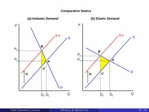
(a) Inelastic Demand (b) Elastic Demand
P
P2
P1
Q1Q2 Q
D
SS+t
B
A
C$t
P2
P1
Q1Q2
P
Q
D
SS+t
B
A
C$t
Comparative Statics
Public Economics Lectures () Effi ciency & Optimal Tax 15 / 81

Tax Policy Implications
With many goods, formula suggests that the most effi cient way toraise tax revenue is:
1 Tax relatively more the inelastic goods (e.g. medical drugs, food)
2 Spread taxes across all goods so as to keep tax rates relatively low onall goods (broad tax base)
Public Economics Lectures () Effi ciency & Optimal Tax 16 / 81

General Model with Income Effects
Marshallian surplus is an ill-defined measure with income effects
Question of interest: how much utility is lost because of tax beyondrevenue transferred to government?
Need units to measure “utility loss”
Introduce expenditure function to translate the utility loss into dollars(money metric)
Public Economics Lectures () Effi ciency & Optimal Tax 17 / 81

Expenditure Function
Fix utility at U and prices at q where q = p + t denotes vector of
tax-inclusive pricesFind bundle that minimizes cost to reach U for q:
e(q,U) = mincq · c s.t. u(c) ≥ U
Let µ denote multiplier on utility constraint
First order conditions given by:
qi = µuciThese generate Hicksian (or compensated) demand fns:
ci = hi (q, u)
Define individual’s loss from tax increase as
e(q1, u)− e(q0, u)Single-valued function → coherent measure of welfare cost, no pathdependencePublic Economics Lectures () Effi ciency & Optimal Tax 18 / 81

Compensating and Equivalent Variation
But where should u be measured?
Consider a price change from q0 to q1
Initial utility:u0 = v(q0,Z )
Utility at new price q1:u1 = v(q1,Z )
Two concepts: compensating (CV ) and equivalent variation (EV ) useu0 and u1 as reference utility levels
Public Economics Lectures () Effi ciency & Optimal Tax 19 / 81

Compensating Variation
Measures utility at initial price level (u0)
Amount agent must be compensated in order to be indifferent abouttax increase
CV = e(q1, u0)− e(q0, u0) = e(q1, u0)− Z
How much compensation is needed to reach original utility level atnew prices?
CV is amount of ex-post cost that must be covered by government toyield same ex-ante utility:
e(q0, u0) = e(q1, u0)− CV
Public Economics Lectures () Effi ciency & Optimal Tax 20 / 81

Equivalent Variation
Measures utility at new price level
Lump sum amount agent willing to pay to avoid tax (at pre-tax prices)
EV = e(q1, u1)− e(q0, u1) = Z − e(q0, u1)
EV is amount extra that can be taken from agent to leave him withsame ex-post utility:
e(q0, u1) + EV = e(q1, u1)
Public Economics Lectures () Effi ciency & Optimal Tax 21 / 81

Effi ciency Cost with Income Effects
Goal: derive empirically implementable formula analogous toMarshallian EB formula in general model with income effects
Existing literature assumes either1 Fixed producer prices and income effects2 Endogenous producer prices and quasilinear utility
With both endogenous prices and income effects, effi ciency costdepends on how profits are returned to consumers
Formulas are very messy and fragile (Auerbach section 3.2)
Public Economics Lectures () Effi ciency & Optimal Tax 22 / 81

Effi ciency Cost Formulas with Income Effects
Derive empirically implementable formulas using Hicksian demand(EV and CV )
Assume p is fixed → flat supply, constant returns to scale
The envelope thm implies that eqi (q, u) = hi , and so:
e(q1, u)− e(q0, u) =∫ q1
q0h(q, u)dq
If only one price is changing, this is the area under the Hicksiandemand curve for that good
Note that optimization implies that
h(q, v(q,Z )) = c(q,Z )
Public Economics Lectures () Effi ciency & Optimal Tax 23 / 81
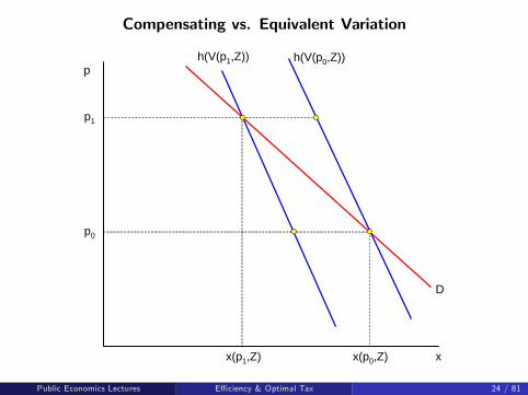
Compensating vs. Equivalent Variation
p
p0
p1
h(V(p1,Z)) h(V(p0,Z))
D
x(p0,Z)x(p1,Z) x
Public Economics Lectures () Effi ciency & Optimal Tax 24 / 81

Compensating vs. Equivalent Variation
p
p0
p1
D
EV
x
h(V(p1,Z)) h(V(p0,Z))
x(p0,Z)x(p1,Z)
Public Economics Lectures () Effi ciency & Optimal Tax 25 / 81

Compensating vs. Equivalent Variation
p
p0
p1
D
CV
x
h(V(p1,Z)) h(V(p0,Z))
x(p0,Z)x(p1,Z)
Public Economics Lectures () Effi ciency & Optimal Tax 26 / 81

Marshallian Surplus
p
p0
p1
D
Marshallian Surplus
x
h(V(p1,Z)) h(V(p0,Z))
x(p0,Z)x(p1,Z)
Public Economics Lectures () Effi ciency & Optimal Tax 27 / 81

Excess Burden
Deadweight burden: change in consumer surplus less tax paid
Equals what is lost in excess of taxes paid
Two measures, corresponding to EV and CV :
EB(u1) = EV − (q1 − q0)h(q1, u1) [Mohring 1971]EB(u0) = CV − (q1 − q0)h(q1, u0) [Diamond and McFadden 1974]
Public Economics Lectures () Effi ciency & Optimal Tax 28 / 81

p
p0
p1
D
x
EBCVEBEV
h(V(p1,Z)) h(V(p0,Z))
x(p1,Z)~
xC(p1,V(p0,Z))~~
~
Public Economics Lectures () Effi ciency & Optimal Tax 29 / 81

p
p0
p1
D
x
Marshallian
h(V(p1,Z)) h(V(p0,Z))
x(p1,Z)~
xC(p1,V(p0,Z))~~
~
Public Economics Lectures () Effi ciency & Optimal Tax 30 / 81
Excess Burden
In general, CV and EV measures of EB will differ
Marshallian measure overstates excess burden because it includesincome effects
Income effects are not a distortion in transactions
Buying less of a good due to having less income is not an effi ciencyloss; no surplus foregone b/c of transactions that do not occur
This is a big deal —DWL arises solely from substitution effects!
Chipman and Moore (1980): CV = EV = Marshallian DWL only withquasilinear utility
Public Economics Lectures () Effi ciency & Optimal Tax 31 / 81

Implementable Excess Burden Formula
Consider increase in tax τ on good 1 to τ + ∆τ
No other taxes in the system
Recall the expression for EB:
EB(τ) = [e(p + τ,U)− e(p,U)]− τh1(p + τ,U)
Second-order Taylor expansion:
MEB = EB(τ + ∆τ)− EB(τ)
' dEBdτ
(∆τ) +12(∆τ)2
d2EBdτ2
Public Economics Lectures () Effi ciency & Optimal Tax 32 / 81

Harberger Trapezoid Formula
dEBdτ
= h1(p + τ,U)− τdh1dτ− h1(p + τ,U)
= −τdh1dτ
d2EBdτ2
= −dh1dτ− τ
d2h1dτ2
Standard practice in literature: assume d 2h1dτ2
(linear Hicksian); notnecessarily well justified because it does not vanish as ∆τ → 0
⇒ MEB = −τ∆τdh1dτ− 12dh1dτ(∆τ)2
Formula equals area of “Harberger trapezoid”using Hicksian demands
Public Economics Lectures () Effi ciency & Optimal Tax 33 / 81

Harberger Formula
Without pre-existing tax, obtain “standard”Harberger formula:
EB = −12dh1dτ(∆τ)2
Observe that first-order term vanishes when τ = 0
A new tax has second-order deadweight burden (proportional to ∆τ2
not ∆τ)
Bottom line: need compensated (substitution) elasticities to computeEB, not uncompensated elasticities
Empirically, need estimates of income and price elasticities (using theslutsky relationship to uncover compensated elasticities)
Public Economics Lectures () Effi ciency & Optimal Tax 34 / 81

Excess Burden with Taxes on Multiple Goods
Previous formulas apply to case with tax on one good
With multiple goods and fixed prices, excess burden of introducing atax τk
EB = −12
τ2kdhkdτk− ∑i 6=k
τiτkdhidτk
Second-order effect in own market, first-order effect from othermarkets with pre-existing taxes
Hard to implement because we need all cross-price elasticities
Complementarity between goods important for excess burdencalculations
Ex: with an income tax, minimize total DWL tax by taxing goodscomplementary to leisure (Corlett and Hague 1953)
Public Economics Lectures () Effi ciency & Optimal Tax 35 / 81

Applied Welfare Analysis with Salience Effects
Chetty, Looney, and Kroft (2009) section 5
Derive partial-equilibrium formulas for incidence and effi ciency costs
Focus here on effi ciency cost analysis
Public Economics Lectures () Effi ciency & Optimal Tax 36 / 81
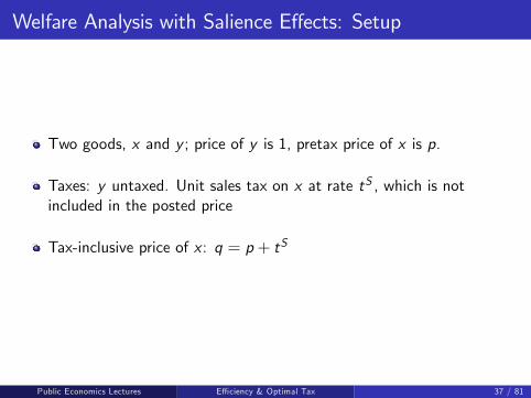
Welfare Analysis with Salience Effects: Setup
Two goods, x and y ; price of y is 1, pretax price of x is p.
Taxes: y untaxed. Unit sales tax on x at rate tS , which is notincluded in the posted price
Tax-inclusive price of x : q = p + tS
Public Economics Lectures () Effi ciency & Optimal Tax 37 / 81

Welfare Analysis with Salience Effects: Setup
Representative consumer has wealth Z and utility u(x) + v(y)
Let{x∗(p, tS ,Z ), y ∗(p, tS ,Z )} denote bundle chosen by afully-optimizing agent
Let {x(p, tS ,Z ), y(p, tS ,Z )} denote empirically observed demands
Place no structure on these demand functions except for feasibility:
(p + tS )x(p, tS ,Z ) + y(p, tS ,Z ) = Z
Public Economics Lectures () Effi ciency & Optimal Tax 38 / 81

Welfare Analysis with Salience Effects: Setup
Price-taking firms use y to produce x with cost fn. c
Firms optimize perfectly. Supply function S(p) defined by:
p = c ′(S(p))
Let εS =∂S∂p ×
pS (p)denote the price elasticity of supply
Public Economics Lectures () Effi ciency & Optimal Tax 39 / 81

Effi ciency Cost with Salience Effects
Define excess burden using EV concept
Excess burden (EB) of introducing a revenue-generating sales tax t is:
EB(tS ) = Z − e(p, 0,V (p, tS ,Z ))− R(p, tS ,Z )
Public Economics Lectures () Effi ciency & Optimal Tax 40 / 81

Preference Recovery Assumptions
A1 Taxes affect utility only through their effects on the chosenconsumption bundle. Agent’s indirect utility given taxes of (tE , tS ) is
V (p, tS ,Z ) = u(x(p, tS ,Z )) + v(y(p, tS ,Z ))
A2 When tax inclusive prices are fully salient, the agent chooses the sameallocation as a fully-optimizing agent:
x(p, 0,Z ) = x∗(p, 0,Z ) = argmaxxu(x) + v(Z − px)
A1 analogous to specification of ancillary condition; A2 analogous torefinement
Public Economics Lectures () Effi ciency & Optimal Tax 41 / 81

Effi ciency Cost with Salience Effects
Two steps in effi ciency calculation:
1 Use price-demand x(p, 0,Z ) to recover utility as in standard model
2 Use tax-demand x(p, tS ,Z )to calculate V (p, tS ,Z ) and EB
Public Economics Lectures () Effi ciency & Optimal Tax 42 / 81

Excess Burden with No Income Effect for Good x ( ∂x∂Z = 0)
Stp,
x0x
)(')0,( xupx =
AB
C
D EG
H
F
1x*1x
I
p0 + tS
xÝp0 , tSÞ
tS /x/tS
tS /x//tS
/x//p
EB p ? 12 Ýt
SÞ 2 /x//tS
/x//p /x//tS
Source: Chetty, Looney, and Kroft (2009)
p0
Public Economics Lectures () Effi ciency & Optimal Tax 43 / 81

Effi ciency Cost: No Income Effects
In the case without income effects ( ∂x∂Z = 0), which implies utility is
quasilinear, excess burden of introducing a small tax tS is
EB(tS ) ' −12(tS )2
∂x/∂tS
∂x/∂p∂x/∂tS
=12(θtS )2
εDp + tS
Inattention reduces excess burden when dx/dZ = 0.
Intuition: tax tS induces behavioral response equivalent to a fullyperceived tax of θtS .
If θ = 0, tax is equivalent to a lump sum tax and EB = 0 becauseagent continues to choose first-best allocation.
Public Economics Lectures () Effi ciency & Optimal Tax 44 / 81

Effi ciency Cost with Income Effects
Same formula, but all elasticities are now compensated:
EB(tS ) ' −12(tS )2
∂xc/∂tS
∂xc/∂p∂xc/∂tS
=12(θc tS )2
εcDp + tS
Compensated price demand: dxc/dp = dx/dp + xdx/dZ
Compensated tax demand: dxc/dtS = dx/dtS + xdx/dZ
Compensated tax demand does not necessarily satisfy Slutskycondition dxc/dtS < 0 b/c it is not generated by utility maximization
Public Economics Lectures () Effi ciency & Optimal Tax 45 / 81
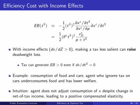
Effi ciency Cost with Income Effects
EB(tS ) ' −12(tS )2
∂xc/∂tS
∂xc/∂p∂xc/∂tS
=12(θc tS )2
εcDp + tS
With income effects (dx/dZ > 0), making a tax less salient can raisedeadweight loss.
Tax can generate EB > 0 even if dx/dtS = 0
Example: consumption of food and cars; agent who ignores tax oncars underconsumes food and has lower welfare.
Intuition: agent does not adjust consumption of x despite change innet-of-tax income, leading to a positive compensated elasticity.
Public Economics Lectures () Effi ciency & Optimal Tax 46 / 81
Brief Look at Optimal Commodity (and Income) Taxation:Introduction
Now combine lessons on incidence and effi ciency costs to analyzeoptimal design of commodity taxes
What is the best way to design taxes given equity and effi ciencyconcerns?
Optimal commodity tax literature focuses on linear (t · x) tax system
Non-linear (t(x)) tax systems considered in income tax literature
Public Economics Lectures () Effi ciency & Optimal Tax 47 / 81

Second Welfare Theorem
Starting point: second-welfare theorem
Can achieve any Pareto-effi cient allocation as a competitiveequilibrium with appropriate lump-sum transfers
Requires same assumptions as first welfare theorem plus one more:1 Complete markets (no externalities)2 Perfect information3 Perfect competition4 Lump-sum taxes/transfers across individuals feasible
If 1-4 hold, equity-effi ciency trade-off disappears and optimal taxproblem is trivial
Simply implement lump sum taxes that meet distributional goals givenrevenue requirement
Problem: informationPublic Economics Lectures () Effi ciency & Optimal Tax 48 / 81

Second Welfare Theorem: Information Constraints
To set the optimal lump-sum taxes, need to know the characteristics(ability) of each individual
But no way to make people reveal their ability at no cost
Incentive to misrepresent skill level
Tax instruments are therefore a fn. of economic outcomes
E.g. income, property, consumption of goods
→ Distorts prices, affecting behavior and generating DWL
Information constraints force us to move from the 1st best world ofthe second welfare theorem to the 2nd best world with ineffi cienttaxation
Cannot redistribute or raise revenue for public goods withoutgenerating effi ciency costs
Public Economics Lectures () Effi ciency & Optimal Tax 49 / 81

Four Central Results in Optimal Tax Theory
1 Ramsey (1927): inverse elasticity rule
2 Diamond and Mirrlees (1971): production effi ciency
3 Atkinson and Stiglitz (1976): no consumption taxation with optimalnon-linear (including lump sum) income taxation
4 Chamley, Judd (1983): no capital taxation in infinite horizon modelsI will briefly mention features of these results but we will not spendthe time to derive them.
Public Economics Lectures () Effi ciency & Optimal Tax 50 / 81

Ramsey (1927) Tax Problem
Government sets taxes on uses of income in order to accomplish twoobjectives:
1 Raise total revenue of amount E
2 Minimize utility loss for agents in economy
Originally a problem set that Pigou assigned Ramsey
Public Economics Lectures () Effi ciency & Optimal Tax 51 / 81

Ramsey Model: Key Assumptions
1 Lump sum taxation prohibited
2 Cannot tax all commodities (leisure untaxed)
3 Production prices fixed (and normalized to one):
pi = 1
⇒ qi = 1+ τi
Public Economics Lectures () Effi ciency & Optimal Tax 52 / 81

Ramsey Model: Setup
One individual (no redistributive concerns) with utility
u(x1, .., xN , l)
subject to budget constraint
q1x1 + ..+ qNxN ≤ wl + Z
Z = non wage income, w = wage rate
Consumption prices are qi
Public Economics Lectures () Effi ciency & Optimal Tax 53 / 81
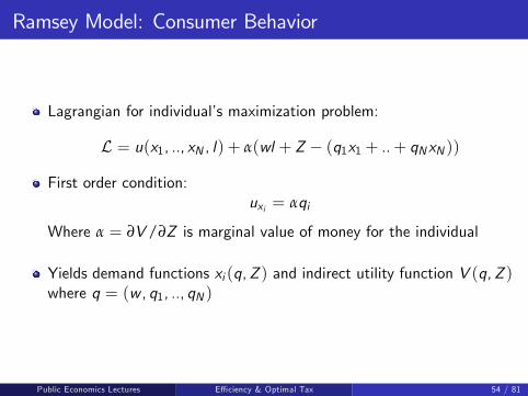
Ramsey Model: Consumer Behavior
Lagrangian for individual’s maximization problem:
L = u(x1, .., xN , l) + α(wl + Z − (q1x1 + ..+ qNxN ))
First order condition:uxi = αqi
Where α = ∂V/∂Z is marginal value of money for the individual
Yields demand functions xi (q,Z ) and indirect utility function V (q,Z )where q = (w , q1, .., qN )
Public Economics Lectures () Effi ciency & Optimal Tax 54 / 81

Ramsey Model: Government’s Problem
Government solves either the maximization problem
maxV (q,Z )
subject to the revenue requirement
τ · x =N
∑i=1
τixi (q,Z ) ≥ E
Or, equivalently, minimize excess burden of the tax system
minEB(q) = e(q,V (q,Z ))− e(p,V (q,Z ))− E
subject to the same revenue requirement
Public Economics Lectures () Effi ciency & Optimal Tax 55 / 81

Ramsey Model: Government’s Problem
For maximization problem, Lagrangian for government is:
LG = V (q,Z ) + λ[∑i
τixi (q,Z )− E ]
⇒ ∂LG∂qi
=∂V∂qi︸︷︷︸
Priv. WelfareLoss to Indiv.
+ λ[ xi︸︷︷︸MechanicalEffect
+∑j
τj∂xj/∂qi︸ ︷︷ ︸BehavioralResponse
] = 0
Using Roy’s identity ( ∂V∂qi= −αxi ):
(λ− α)xi + λ ∑j
τj∂xj/∂qi = 0
Public Economics Lectures () Effi ciency & Optimal Tax 56 / 81

Ramsey Optimal Tax Formula
Optimal tax rates satisfy system of N equations and N unknowns:
∑j
τj∂xj∂qi
= −xiλ(λ− α)
Same formula can be derived using a perturbation argument, which ismore intuitive
Public Economics Lectures () Effi ciency & Optimal Tax 57 / 81
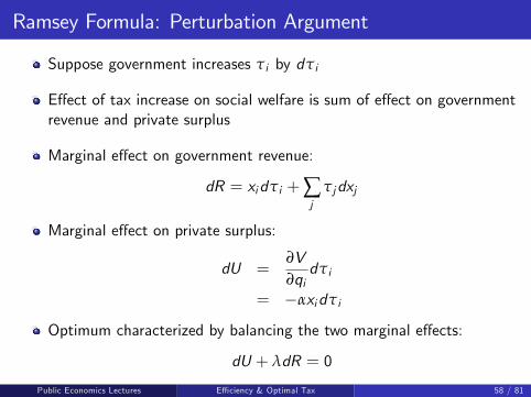
Ramsey Formula: Perturbation Argument
Suppose government increases τi by dτi
Effect of tax increase on social welfare is sum of effect on governmentrevenue and private surplus
Marginal effect on government revenue:
dR = xidτi +∑j
τjdxj
Marginal effect on private surplus:
dU =∂V∂qidτi
= −αxidτi
Optimum characterized by balancing the two marginal effects:
dU + λdR = 0
Public Economics Lectures () Effi ciency & Optimal Tax 58 / 81

Ramsey Formula: Compensated Elasticity Representation
Rewrite in terms of Hicksian elasticities to obtain further intuitionusing Slutsky equation:
∂xj/∂qi = ∂hj/∂qi − xi∂xj/∂Z
Substitution into formula above yields:
(λ− α)xi + λ ∑j
τj [∂hj/∂qi − xi∂xj/∂Z ] = 0
⇒ 1xi
∑j
τj∂hi∂qj
= − θ
λ
where θ = λ− α− λ ∂∂Z (∑j τjxj )
Public Economics Lectures () Effi ciency & Optimal Tax 59 / 81

Ramsey Formula: Compensated Elasticity Representation
θ is independent of i and measures the value for the government ofintroducing a $1 lump sum tax
θ = λ− α− λ∂(∑j
τjxj )/∂Z
Three effects of introducing a $1 lumpsum tax:1 Direct value for the government is λ2 Loss in welfare for the individual is α3 Behavioral effect → loss in tax revenue of ∂(∑j τjxj )/∂Z
Can demonstrate that θ > 0⇒ λ > α at the optimum using Slutskymatrix
Public Economics Lectures () Effi ciency & Optimal Tax 60 / 81

Intuition for Ramsey Formula: Index of Discouragement
1xi
∑j
τj∂hi∂qj
= − θ
λ
Suppose revenue requirement E is small so that all taxes are also small
Then tax τj on good j reduces consumption of good i (holding utilityconstant) by approximately
dhi = τj∂hi∂qj
Numerator of LHS: total reduction in consumption of good i
Dividing by xi yields % reduction in consumption of each good i =“index of discouragement”of the tax system on good i
Ramsey tax formula says that the indexes of discouragements must beequal across goods at the optimum
Public Economics Lectures () Effi ciency & Optimal Tax 61 / 81

Special Case 1: Inverse Elasticity Rule
Introducing elasticities, we can write formula as:
N
∑j=1
τj1+ τj
εcij =θ
λ
Consider special case where εij = 0 if i 6= j
Slutsky matrix is diagonal
Obtain classic inverse elasticity rule:
τi1+ τi
=θ
λ
1εii
Public Economics Lectures () Effi ciency & Optimal Tax 62 / 81

Special Case 2: Uniform Taxation
Suppose εij = 0 if i 6= j and εxi ,w =∂hiwwhiconstant
Using following identity, ∑j
∂hi∂qjqj +
∂hi∂w w = 0, we obtain
∂hi∂qiqi = −
∂hi∂ww
Proof of identity (J good economy, no labor):
∑j
∂hi∂qjqj = ∑
j 6=i
∂hj∂qiqj +
∂hi∂qiqi
= ∑j 6=i
∂hjqj∂qi
+∂hiqi∂qi− hi
=∂e∂qi− hi = 0
Public Economics Lectures () Effi ciency & Optimal Tax 63 / 81

Special Case 2: Uniform Taxation
Then immediately obtain
1xi
τi = − θ
λ
1∂hi∂qi
=θ
λ
1∂hi∂w w
τiqi
=θ
λ
1∂hi∂w
wxi
=θ
λεxi ,w
With constant εxi ,w ,τiqiis constant → uniform taxation
Corlett and Hague (1953): 3 good model, uniform tax optimal if allgoods are equally complementary with labor (and labor is untaxed)
More generally, lower taxes for goods complementary to labor
Public Economics Lectures () Effi ciency & Optimal Tax 64 / 81

Ramsey Formula: Limitations
Ramsey solution: tax inelastic goods to minimize effi ciency costs
But does not take into account redistributive motives
Presumably necessities are more inelastic than luxuries
Therefore, optimal Ramsey tax system is likely to be regressive
Diamond (1975) extends Ramsey model to take redistributive motivesinto account
Public Economics Lectures () Effi ciency & Optimal Tax 65 / 81

Diamond and Mirrlees (1971)
Previous analysis assumed fixed producer prices
Diamond and Mirrlees (1971) relax this assumption by modellingproduction
Two major results
1 Production effi ciency: even in an economy where first-best isunattainable, optimal policy maintains production effi ciency
2 Characterize optimal tax rates with endogenous prices and show thatRamsey rule can be applied
Public Economics Lectures () Effi ciency & Optimal Tax 66 / 81

Lipsey and Lancaster (1956): Theory of the Second Best
Standard optimal policy results only hold with single deviation fromfirst best
Ex: Ramsey formulas invalid if there are pre-existing distortions,imperfect competition, etc.
In second-best, anything is possible
Policy changes that would increase welfare in a model with a singledeviation from first best need not do so in second-best
Ex: tariffs can improve welfare by reducing distortions in other part ofeconomy
Destructive result for welfare economics
Public Economics Lectures () Effi ciency & Optimal Tax 67 / 81

Diamond and Mirrlees: Production Effi ciency
Diamond and Mirrlees result was an advance because it showed ageneral policy lesson even in second-best environment
Example: Suppose government can tax consumption goods and alsoproduces some goods on its own (e.g. postal services)
May have intuition that government should try to generate profits inpostal services by increasing the price of stamps
This intuition is wrong: optimal to have no distortions in productionof goods
Bottom line: only tax goods that appear directly in agent’s utilityfunctions
Should not distort production decisions via taxes on intermediategoods, tariffs, etc.
Public Economics Lectures () Effi ciency & Optimal Tax 68 / 81

Policy Consequences: Public Sector Production
Public sector production should be effi cient
If there is a public sector producing some goods, it should:
Face the same prices as the private sector
Choose production with the unique goal of maximizing profits, notgenerating government revenue
Ex. postal services, electricity, health care, ...
Public Economics Lectures () Effi ciency & Optimal Tax 69 / 81

Policy Consequences: No Taxation of Intermediate Goods
Intermediate goods: goods that are neither direct inputs or outputsto indiv. consumption
Taxes on transactions between firms would distort production
Public Economics Lectures () Effi ciency & Optimal Tax 70 / 81

Policy Consequences: No Taxation of Intermediate Goods
Computers:
Sales to firms should be untaxedBut sales to consumers should be taxed
In practice, tax policy often follows precisely the opposite rule
Ex. Diesel fuel tax studied by Marion and Muehlegger (2008)
Public Economics Lectures () Effi ciency & Optimal Tax 71 / 81

Diamond and Mirrlees Model: Key Assumptions
Result hinges on key assumptions about govt’s ability to:
1 Set a full set of differentiated tax rates on each input and output
2 Tax away fully pure profits (or production is constant-returns-to-scale)
A2 rules out improving welfare by taxing profitable industries toimprove distribution at expense of production effi ciency
These assumptions effectively separate the production andconsumption problems
Public Economics Lectures () Effi ciency & Optimal Tax 72 / 81

Diamond and Mirrlees Result: Limitations
Practical relevance of the result is a bit less clear
Ex. Assumption 1 is not realistic (Naito 1999)
Skilled and unskilled labor inputs ought to be differentiated
Not the case in current income tax system
In such cases, may be optimal to:
1 Subsidize low skilled intensive industries
2 Set tariffs on low skilled intensive imported goods (to protect domesticindustry)
Public Economics Lectures () Effi ciency & Optimal Tax 73 / 81

Mirrlees 1971: Optimal Income Tax Problem IncorporatingBehavioral Responses
Standard labor supply model: Individual maximizes
u(c , l) s.t. c = wl − T (wl)
where c is consumption, l labor supply, w wage rate, T (.) income tax
Individuals differ in ability w distributed with density f (w)
Govt social welfare maximization: Govt maximizes
SWF =∫G (u(c , l))f (w)dw)
s.t. resource constraint∫T (wl)f (w)dw ≥ E
and individual FOC w(1− T ′)uc + ul = 0
where G (.) is increasing and concave
Public Economics Lectures () Effi ciency & Optimal Tax 74 / 81

Mirrlees 1971: Results
Optimal income tax trades-off redistribution and effi ciency
T (.) < 0 at bottom (transfer)
T (.) > 0 further up (tax) [full integration of taxes/transfers]
Mirrlees formulas are a complex fn. of primitives, with only a fewgeneral results
1 0 ≤ T ′(.) ≤ 1, T ′(.) ≥ 0 is non-trivial and rules out EITC [Seade1976]
2 Marginal tax rate T ′(.) should be zero at the top if skill distributionbounded [Sadka-Seade]
Public Economics Lectures () Effi ciency & Optimal Tax 75 / 81

Mirrlees: Subsequent Work
Mirrlees model had a profound impact on information economics
Ex. models with asymmetric information in contract theory
But until late 1990s, Mirrlees had little impact on practical tax policy
Recently, Mirrlees model connected to empirical literature
Diamond (1998), Piketty (1997), and Saez (2001)
See Bernheim paper on Saez’s work for one nice description.
Public Economics Lectures () Effi ciency & Optimal Tax 76 / 81

Commodity vs. Income Taxation
Now combine commodity tax and income tax results to analyzeoptimal combination of policies
In practice, government levies differential commodity taxes along withnon-linear income tax
1 Exempts some goods (food, education, health) from sales tax
2 Imposes additional excise taxes on some goods (cars, gasoline, luxurygoods)
3 Imposes capital income taxes
What is the best combination of taxes?
Public Economics Lectures () Effi ciency & Optimal Tax 77 / 81

Atkinson-Stiglitz: Intuition
With separability and homogeneity, conditional on earnings z ,consumption choices c = (c1, .., cK ) do not provide any informationon ability
Differentiated commodity taxes t1, .., tK create a tax distortion withno benefit
Better to do all the redistribution with the individual income tax
With only linear income taxation (Diamond-Mirrlees 1971, Diamond1975), diff. commodity taxation can be useful to “non-linearize” thetax system
But not if Engel curves for each ck are linear in y (Deaton 1981)
Public Economics Lectures () Effi ciency & Optimal Tax 78 / 81

Failures of A-S Assumptions
If higher ability consume more of good k than lower ability people,then taxing good k is desirable. Examples:
1 High ability people have a relatively higher taste for good k (at a givenincome)
Luxury chocolates or museums; violates homogeneous v (c) assumption
2 Good k is positively related to leisure (consumption of k increaseswhen leisure increases at a given income)
Tax on travel, subsidy on computers and work related expenses
In general Atkinson-Stiglitz assumptions are viewed as a good startingplace for most goods
Public Economics Lectures () Effi ciency & Optimal Tax 79 / 81

Chamley-Judd: Capital Taxation
Judd (1985) and Chamley (1986) examine capital taxation
Consider a Ramsey model where govt. is limited to lineardistortionary taxes
Result: optimal capital tax converges to zero in long run
Intuition: DWL rises with square of tax rate
With non-zero capital tax, have an infinite price distortion between c0and ct as t → ∞
Undesirable to have such large distortions on some margins
Public Economics Lectures () Effi ciency & Optimal Tax 80 / 81
The New Dynamic Public Finance Literature(Kocherlakota, Werning, Golosov, Tsyvinski, amongothers)
Maybe capital taxes shouldn’t be zero for everyone.
When preferences are separable between consumption and leisure, thewealthy in (t+1) are harder to motivate.
At the margin, therefore, good tax systems will deter wealthaccumulation from period t to period (t+1) to provide better workincentives in the later period.
More generally, when people are working hard, you want low asset taxrates. When people have little labor income, you want high asset taxrates.
In general, results on optimal capital income taxation are prettyfragile.
Public Economics Lectures () Effi ciency & Optimal Tax 81 / 81


