Public economics

c©Mattias K. Polborn

prepared as lecture notes for Economics 511

MSPE program

University of Illinois

Department of Economics

Version: November 27, 2012

Contents

I Competitive markets and welfare theorems 6

1 Welfare economics 7

1.1 Introduction . . . . . . . . . . . . . . . . . . . . . . . . . . . . . . . . . . . . . . . 7

1.2 Edgeworth boxes and Pareto efficiency . . . . . . . . . . . . . . . . . . . . . . . . 8

1.3 Exchange . . . . . . . . . . . . . . . . . . . . . . . . . . . . . . . . . . . . . . . . 12

1.4 First theorem of welfare economics . . . . . . . . . . . . . . . . . . . . . . . . . . 14

1.5 Efficiency with production . . . . . . . . . . . . . . . . . . . . . . . . . . . . . . . 15

1.6 Application: Emissions reduction . . . . . . . . . . . . . . . . . . . . . . . . . . . 19

1.7 Second theorem of welfare economics . . . . . . . . . . . . . . . . . . . . . . . . . 24

1.8 Application: Subsidizing bread to help the poor? . . . . . . . . . . . . . . . . . . 25

1.9 Limitations of efficiency results . . . . . . . . . . . . . . . . . . . . . . . . . . . . 27

1.9.1 Redistribution . . . . . . . . . . . . . . . . . . . . . . . . . . . . . . . . . 28

1.9.2 Market failure . . . . . . . . . . . . . . . . . . . . . . . . . . . . . . . . . 28

1.10 Utility theory and the measurement of benefits . . . . . . . . . . . . . . . . . . . 29

1.10.1 Utility maximization and preferences . . . . . . . . . . . . . . . . . . . . . 30

1.10.2 Cost-benefit analysis . . . . . . . . . . . . . . . . . . . . . . . . . . . . . . 33

1.11 Partial equilibrium measures of welfare . . . . . . . . . . . . . . . . . . . . . . . . 39

1.12 Applications of partial welfare measures . . . . . . . . . . . . . . . . . . . . . . . 42

1.12.1 Welfare effects of an excise tax . . . . . . . . . . . . . . . . . . . . . . . . 42

1.12.2 Welfare effect of a subsidy . . . . . . . . . . . . . . . . . . . . . . . . . . . 43

1.12.3 Price ceiling . . . . . . . . . . . . . . . . . . . . . . . . . . . . . . . . . . . 43

1.12.4 Agricultural subsidies and excess production . . . . . . . . . . . . . . . . 45

1.13 Non-price-based allocation systems . . . . . . . . . . . . . . . . . . . . . . . . . . 46

II Market failure 50

2 Imperfect competition 51

2.1 Introduction . . . . . . . . . . . . . . . . . . . . . . . . . . . . . . . . . . . . . . . 51

2.2 Monopoly in an Edgeworth box diagram . . . . . . . . . . . . . . . . . . . . . . . 52

1

2.3 The basic monopoly problem . . . . . . . . . . . . . . . . . . . . . . . . . . . . . 53

2.4 Two-part pricing . . . . . . . . . . . . . . . . . . . . . . . . . . . . . . . . . . . . 54

2.4.1 A mathematical example of a price-discriminating monopolist . . . . . . . 56

2.5 Policies towards monopoly . . . . . . . . . . . . . . . . . . . . . . . . . . . . . . . 58

2.6 Natural monopolies . . . . . . . . . . . . . . . . . . . . . . . . . . . . . . . . . . . 60

2.7 Cross subsidization and Ramsey pricing . . . . . . . . . . . . . . . . . . . . . . . 61

2.8 Patents . . . . . . . . . . . . . . . . . . . . . . . . . . . . . . . . . . . . . . . . . 63

2.9 Application: Corruption . . . . . . . . . . . . . . . . . . . . . . . . . . . . . . . . 63

2.10 Introduction to game theory . . . . . . . . . . . . . . . . . . . . . . . . . . . . . . 65

2.11 Cournot oligopoly . . . . . . . . . . . . . . . . . . . . . . . . . . . . . . . . . . . 68

3 Public Goods 71

3.1 Introduction and classification . . . . . . . . . . . . . . . . . . . . . . . . . . . . . 71

3.2 Efficient provision of a public good . . . . . . . . . . . . . . . . . . . . . . . . . . 73

3.3 Private provision of public goods . . . . . . . . . . . . . . . . . . . . . . . . . . . 74

3.4 Clarke–Groves mechanism . . . . . . . . . . . . . . . . . . . . . . . . . . . . . . . 77

3.5 Applications . . . . . . . . . . . . . . . . . . . . . . . . . . . . . . . . . . . . . . . 80

3.5.1 Private provision of public goods: Open source software . . . . . . . . . . 80

3.5.2 Importance of public goods for human history: “Guns, germs and steel” . 80

4 Externalities 82

4.1 Introduction . . . . . . . . . . . . . . . . . . . . . . . . . . . . . . . . . . . . . . . 82

4.2 “Pecuniary” vs. “non-pecuniary” externalities . . . . . . . . . . . . . . . . . . . . 82

4.3 Application: Environmental Pollution . . . . . . . . . . . . . . . . . . . . . . . . 83

4.3.1 An example of a negative externality . . . . . . . . . . . . . . . . . . . . . 83

4.3.2 Merger . . . . . . . . . . . . . . . . . . . . . . . . . . . . . . . . . . . . . . 84

4.3.3 Assigning property rights . . . . . . . . . . . . . . . . . . . . . . . . . . . 85

4.3.4 Pigou taxes . . . . . . . . . . . . . . . . . . . . . . . . . . . . . . . . . . . 88

4.4 Positive externalities . . . . . . . . . . . . . . . . . . . . . . . . . . . . . . . . . . 89

4.5 Resources with non-excludable access: The commons . . . . . . . . . . . . . . . . 90

5 Asymmetric Information 92

5.1 Introduction . . . . . . . . . . . . . . . . . . . . . . . . . . . . . . . . . . . . . . . 92

5.2 Example: The used car market . . . . . . . . . . . . . . . . . . . . . . . . . . . . 93

5.2.1 Akerlof’s model of a used car market . . . . . . . . . . . . . . . . . . . . . 93

5.2.2 Adverse selection and policy . . . . . . . . . . . . . . . . . . . . . . . . . . 94

5.3 Signaling through education . . . . . . . . . . . . . . . . . . . . . . . . . . . . . 95

5.4 Moral Hazard . . . . . . . . . . . . . . . . . . . . . . . . . . . . . . . . . . . . . . 96

5.4.1 A principal-agent model of moral hazard . . . . . . . . . . . . . . . . . . . 96

2

5.4.2 Moral hazard and policy . . . . . . . . . . . . . . . . . . . . . . . . . . . . 101

III Social choice and political economy 102

6 The Social Choice Approach to Political Decision Making 103

6.1 Introduction . . . . . . . . . . . . . . . . . . . . . . . . . . . . . . . . . . . . . . . 103

6.2 Social preference aggregation . . . . . . . . . . . . . . . . . . . . . . . . . . . . . 104

6.2.1 Review of preference relations . . . . . . . . . . . . . . . . . . . . . . . . . 105

6.2.2 Preference aggregation . . . . . . . . . . . . . . . . . . . . . . . . . . . . . 107

6.3 Desirable properties for preference aggregation mechanisms: Arrow’s axioms . . . 110

6.3.1 Examples of social aggregation procedures . . . . . . . . . . . . . . . . . . 115

6.4 Statement and proof of Arrow’s theorem . . . . . . . . . . . . . . . . . . . . . . . 118

6.5 Interpretation of Arrow’s Theorem . . . . . . . . . . . . . . . . . . . . . . . . . . 121

6.6 Social choice functions (incomplete) . . . . . . . . . . . . . . . . . . . . . . . . . 123

6.7 Gibbard-Satterthwaite Theorem . . . . . . . . . . . . . . . . . . . . . . . . . . . . 125

7 Direct democracy and the median voter theorem 128

7.1 Introduction . . . . . . . . . . . . . . . . . . . . . . . . . . . . . . . . . . . . . . . 128

7.2 Single-peaked preferences . . . . . . . . . . . . . . . . . . . . . . . . . . . . . . . 128

7.3 Median voter theorem . . . . . . . . . . . . . . . . . . . . . . . . . . . . . . . . . 130

7.3.1 Statement of the theorem . . . . . . . . . . . . . . . . . . . . . . . . . . . 130

7.3.2 Example: Voting on public good provision . . . . . . . . . . . . . . . . . . 131

7.4 Multidimensionality and the median voter theorem . . . . . . . . . . . . . . . . . 134

8 Candidate competition 139

8.1 Introduction . . . . . . . . . . . . . . . . . . . . . . . . . . . . . . . . . . . . . . . 139

8.2 The Downsian model of office-motivated candidates . . . . . . . . . . . . . . . . . 141

8.3 Policy-motivated candidates with commitment . . . . . . . . . . . . . . . . . . . 147

8.4 Policy-motivated candidates without commitment: The citizen-candidate model . 149

8.5 Probabilistic voting . . . . . . . . . . . . . . . . . . . . . . . . . . . . . . . . . . . 152

8.6 Differentiated candidates . . . . . . . . . . . . . . . . . . . . . . . . . . . . . . . . 154

9 Endogenous participation 157

9.1 Introduction . . . . . . . . . . . . . . . . . . . . . . . . . . . . . . . . . . . . . . . 157

9.2 The model setup . . . . . . . . . . . . . . . . . . . . . . . . . . . . . . . . . . . . 157

9.3 A simple example: Voting as public good provision . . . . . . . . . . . . . . . . . 158

9.4 Analysis of the general costly voting model . . . . . . . . . . . . . . . . . . . . . 160

9.4.1 Positive analysis . . . . . . . . . . . . . . . . . . . . . . . . . . . . . . . . 160

9.4.2 Welfare analysis . . . . . . . . . . . . . . . . . . . . . . . . . . . . . . . . 164

3

9.5 Costly voting in finite electorates . . . . . . . . . . . . . . . . . . . . . . . . . . . 165

Index . . . . . . . . . . . . . . . . . . . . . . . . . . . . . . . . . . . . . . . . . . . . . 168

4

Preface

This file contains lecture notes that I have written for a course in Public Economics in the

Master of Science in Policy Economics at the University of Illinois at Urbana-Champaign. I

have taught this course four times before, and this version for the 2009 course is probably

reasonably complete: Students in my class may want to print this version, and while I will

update this material during the fall semester, I expect most of the updates to be minor, not

requiring you to reprint material extensively. If there are any major revisions, I will announce

this in class.

This class covers the core topics of public economics, in particular welfare economics; reasons

for and policies dealing with market failures such as imperfect competition, externalities and

public goods, and asymmetric information. In the last part, I provide an introduction to theories

of political economy. In my class, this book and the lectures will be supplemented by additional

readings (often for case studies). These readings will be posted on the course website.

Relative to previous years, I have added, rewritten or rearranged some sections in Parts 1

and 2, but most significantly, in Part 3. This is also the part where most remains to be done

for future revisions.

The reason for why I have chosen to write this book as a supplement to my lectures is

that I could not find a completely satisfying textbook for this class. Many MSPE students are

accomplished government or central bank officials from a number of countries, who return to

university studies after working some time in their respective agencies. They bring with them a

unique experiences in the practice of public economics, so that most undergraduate texts would

not be sufficiently challenging (and would under-use the students’ experiences and abilities). On

the other hand, most graduate texts are designed for graduate students aiming for a Ph.D in

economics. These books are often too technical to be accessible.

My objective in selecting course materials, and in writing these lecture notes, is to teach the

fundamental concepts of allocative efficiency, market failure and state intervention in markets in

a non-technical way, emphasizing the economic intuition over mathematical details. However,

non-technical here certainly does not mean “easy”, and familiarity with microeconomics and

optimization techniques, as taught in the core microeconomics class of the MSPE program, is

assumed. The key objective is to achieve an understanding of concepts. Ideally, students should

5

understand them so thoroughly that they are able to apply these concepts to analyze problems

that differ from those covered in class, and later, to problems in their work environment.

Several cohorts of students have read this text and have given me their feedback (many

thanks!), and I always appreciate additional feedback on anything from typos to what you like

or dislike in the organization of the material.

Finally, if you are a professor at another university who would like to use this book or parts

of it in one of your courses, you are welcome to do so for free, but I would be happy if you let

me know through email to polborn@uiuc.edu.

Mattias K. Polborn

6

Part I

Competitive markets and welfare

theorems

7

Chapter 1

Welfare economics

1.1 Introduction

The central question of public economics and the main emphasis of our course is the question of

whether and how the government should intervene in the market. To answer this question, we

need some benchmark measure against which we can compare the outcome with and without

government interference.

In this chapter, we develop a model of a very simple market whose equilibrium is “optimal”

(in a way that we will define precisely). The following chapters will then modify some assump-

tions of this simple model, generating instances of market failure, in which the outcome in a

private market is not optimal. In these cases, an intervention by the government can increase

the efficiency of the market allocation. When correcting market failures, the state often takes

actions that benefit some and harm other people, so we need a measure of how to compare these

desirable and undesirable effects. Hence, we need an objective function for the state.

We start this chapter by using an Edgeworth box exchange model to define Pareto opti-

mality as efficiency criterion, and prove the First Theorem of Welfare Economics: A market

equilibrium in a simple competitive exchange economy is Pareto efficient. This result is robust

to incorporating production in the model, and, under certain conditions, the converse of the

First Theorem is also true: Each Pareto optimum can be supported as a market equilibrium if

we distribute the initial endowments appropriately. However, we also points out the limitations

of the efficiency results.

The First and Second Theorems of Welfare Economics are derived in a general equilibrium

framework. While theoretically nice, general equilibrium models are often not very tractable

when, in reality, there are thousands of different markets. Often, we are particularly interested

with the consequences of actions in one particular market, and in this case, partial equilibrium

models are helpful, and we analyze several applications.

Pareto optimality, our measure of efficiency, is in many respects a useful concept. However,

8

when the government intervenes in a market (or, indeed, implements any policy), it is very rare

that all individuals in society are made better off, or that all could be made better off with some

other feasible policy. Most of the time, a policy benefits some people and harms others. In these

cases, it is useful to have a way to compare the size of the gains of winners with the size of the

costs of losers.

In the 18th century, “utilitarian” philosophers have suggested that the objective of the state

should be to achieve the highest possible utility for the largest number of people. Unfortunately,

utility as defined by modern microeconomic theory is an ordinal rather than cardinal concept,

and so the sum of different people’s utilities is not a useful concept. We explain why this is the

case and, more constructively, how we can make utility gains and losses comparable by the use

of compensating and equivalent variation measures.

Finally, we also discuss other methods of allocating goods, apart from selling them. For

example, in many communist economies, some goods were priced considerably below the price

that people were willing to pay, but there was only a limited supply available at the low price,

with allocation often determined through queuing.

1.2 Edgeworth boxes and Pareto efficiency

Economists distinguish positive and normative economic models. Positive models explain how

the economy (or some part of the economy) works; for example, a model that analyzes which

effect rent control has on the supply of new housing or on how often people move is a positive

model. In contrast, normative models analyze how a given objective should be reached in an

optimal way; for example, optimal tax models that analyze how the state should raise a given

amount of revenue while minimizing the total costs of citizens are examples of normative models.

One important ingredient in every normative model is the concept of optimality: What

should be the state’s objective when choosing its policy? One very important criterion in

economics is called Pareto optimality or Pareto efficiency. We will develop this concept with the

help of some graphs. Figure 1.1 is called an Edgeworth Box. It has the following interpretation.

Our economy is populated by two people, A and B, and there are two types of goods, clothing

and food. The total amount of clothing available in the economy is measured on the horizontal

axis of the Edgeworth box, and similarly, the total amount of food is measured as the height of

the box.

A point in the Edgeworth box can be interpreted as an allocation of the two goods to the

two individuals. For example, the bullet in the box means that A gets CA units of clothing

and FA units of food, while the remaining units of clothing (CB) and food (FB) initially go to

individual B.

We can also add the two individuals’ preferences, in the form of indifference curves, to the

graphic. The two regularly-shaped (convex) curves are indifference curves for A, and the two

9

A

B

C

F

•

CA

FA

FB

CB

Figure 1.1: Allocations in an Edgeworth box

other ones are indifference curves of individual B. Note that individual B’s indifference curves

“stand on the head” in the sense that B likes allocations that are to the southwest better, and

so, seen from B’s point of view, his indifference curves are just as “regularly-shaped” (convex)

as A’s ones. Note that the indifference curves for both individuals are not restricted to the

allocations inside the box; the individuals’ preferences are defined for all possible positive levels

of consumption, not restricted to what is available in this particular economy. The allocation

that is marked with the dot in the previous figure is called an initial endowment. It is interpreted

as the original property rights to goods that the two individuals have before they possibly trade

with each other and exchange goods.

Consider now the two indifference curves, one for A and the other one for B, that pass through

the initial endowment marked X in Figure 1.2. The area that is above A’s indifference curve

consists of all those allocations that make A better off than the initial endowment. Similarly, the

area “below” B’s indifference curve (which is actually above B’s indifference curve, when seen

from B’s point of view) contains all allocations that are better for B than the initial allocation.

Hence, the lens-shaped, shaded area that is included by the two indifference curves that pass

through the initial endowment is the area of allocations that are better for both A and B than

the initial endowment.

If A and B exchange goods, and specifically if A gives some clothing to B in exchange for

some food such that they move to a point like Y in the shaded area, then both individuals will

be better off than before. Such an exchange that makes all parties involved better off (or, at

least one party better off, without harming the other party) is called a Pareto improvement. We

also say that allocation Y is Pareto better than allocation X.

10

A

B

C

F

•X

• Y

•Z

Figure 1.2: Making A better off without making B worse off

Not all allocations in an Edgeworth box can be Pareto compared in the sense that either

one of them is Pareto better than the other. Consider, for example, allocation Z in Figure 1.2.

Individual A has a higher utility in Z than in X (or in Y , for that matter), while individual B

has a lower utility in Z than in X (or Y ). Therefore, X and Z (and Y and Z) are “not Pareto

comparable”.

We now turn to the notion of Pareto efficiency. Whenever an initial endowment leaves

the possibility of making all individuals better off by redistributing the available goods among

them, then the initial allocation is inefficient. In particular, all allocations in the interior of

the box that have the property that two indifference curves intersect there (i.e., cut each other)

are inefficient, in this sense that all individuals could be simultaneously better off than in that

allocation.

However, there are also allocations, starting from which a further improvement for both

individuals is impossible, and such an allocation is called Pareto efficient (or, synonymously, a

Pareto optimum). Consider allocation P in Figure 1.3.

P is Pareto efficient, because starting from P, there is no possibility to reallocate the goods

and thereby to make both individuals better off. To see this, note that the area of allocations

that are better for A (to the northeast of A’s indifference curve that passes through P ) and the

area of allocations that are better for B (to the southwest of B’s indifference curve that passes

through P ) do not intersect.

Figure 1.3 suggests that those points in the interior of the Edgeworth box where A’s and

B’s indifference curves are tangent to each other (i.e. just touch each other, without cutting

11

A

B

C

F •P•P′

•P ′′

Figure 1.3: Pareto efficient allocations

through each other) are Pareto optima.1 This is in fact correct as long as both individuals have

convex shaped indifference curves (as usually).

However, even if indifference curves are regularly-shaped, there may be allocations at the

edges of the box that are Pareto optima, even though indifference curves are not tangent to

each other there. The decisive feature of a Pareto optimum is that the intersection of the sets

of allocations that are preferred by A and B is empty.

Although most allocations in an Edgeworth box are Pareto inefficient, there are also (usually)

many Pareto optima. For example, in Figure 1.3, P ′ and P ′′ are also Pareto optima. Obviously,

there is no Pareto comparison possible among Pareto optima: No Pareto optimum is Pareto

better than another Pareto optimum, because if it were, than the latter would not be a Pareto

optimum. In Figure 1.3, P is better than P ′′ and worse than P ′ for A, and the opposite holds

for B.

In fact, all Pareto optima can be connected and lie on a curve that connects the southwest

corner with the northeast corner of the Edgeworth box; see Figure 1.4. This curve is called the

contract curve. The reason for this name is as follows: When the individuals can trade with

each other, then they will likely end up on some point on the contract curve; they will not

stop trading with each other before the contract curve is reached, because there would still be

potential gains from trading for both parties that would be left unexploited.

Both A and B must agree to any exchange, and they will only do so if the resulting allocation

is better for both of them. Furthermore, if they are rational, they will exhaust all possible gains

1The plural of “optimum” is not “optimums”, but rather “optima”, a plural form in Latin. The same plural

form appears for “maximum”, “minimum” and a number of other words ending -um.

12

A

B

C

F •P

•P′

•P ′′ •X

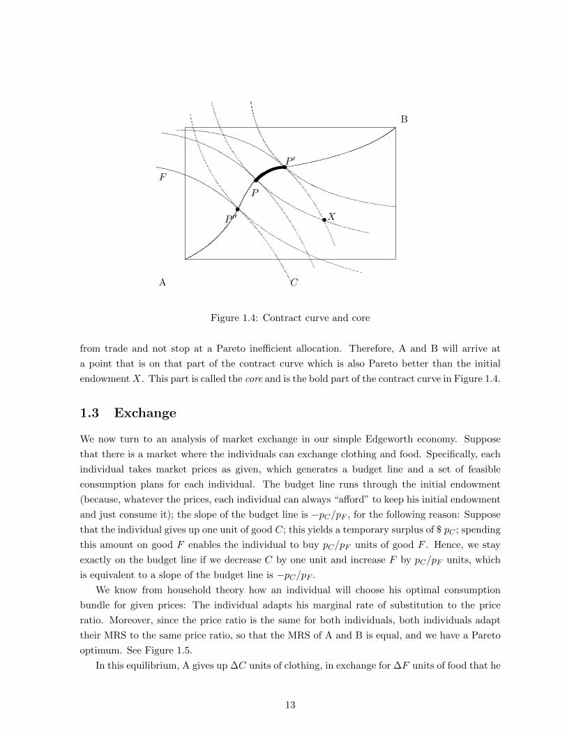
Figure 1.4: Contract curve and core

from trade and not stop at a Pareto inefficient allocation. Therefore, A and B will arrive at

a point that is on that part of the contract curve which is also Pareto better than the initial

endowment X. This part is called the core and is the bold part of the contract curve in Figure 1.4.

1.3 Exchange

We now turn to an analysis of market exchange in our simple Edgeworth economy. Suppose

that there is a market where the individuals can exchange clothing and food. Specifically, each

individual takes market prices as given, which generates a budget line and a set of feasible

consumption plans for each individual. The budget line runs through the initial endowment

(because, whatever the prices, each individual can always “afford” to keep his initial endowment

and just consume it); the slope of the budget line is −pC/pF , for the following reason: Suppose

that the individual gives up one unit of good C; this yields a temporary surplus of $ pC ; spending

this amount on good F enables the individual to buy pC/pF units of good F . Hence, we stay

exactly on the budget line if we decrease C by one unit and increase F by pC/pF units, which

is equivalent to a slope of the budget line is −pC/pF .

We know from household theory how an individual will choose his optimal consumption

bundle for given prices: The individual adapts his marginal rate of substitution to the price

ratio. Moreover, since the price ratio is the same for both individuals, both individuals adapt

their MRS to the same price ratio, so that the MRS of A and B is equal, and we have a Pareto

optimum. See Figure 1.5.

In this equilibrium, A gives up ∆C units of clothing, in exchange for ∆F units of food that he

13

A

B

C

F

•�

∆C

∆F

Figure 1.5: Edgeworth Box and equilibrium prices

gets from B. Note that the optimal consumption chosen by A brings us to the same allocation

in the Edgeworth box as the optimal consumption chosen by B.2 In fact, this is a necessary

property of equilibrium: If the two individuals were to attempt to “choose” their consumption

such that different allocations in the Edgeworth box emerged, there is an excess demand for one

and an excess supply for the other good.

Consider Figure 1.6 in which there are disequilibrium prices. Both A and B would try to

adapt their MRS to the price ratio of −pC/pF = −1, but achieve this at different points. B’s

optimal point at the initial endowment, which means that B neither wants to buy nor to sell

any of his endowment. A, on the other hand, wants to sell some clothes and buy some food. On

aggregate, this means that there is an excess demand in the food market and an excess supply in

the clothing market. As a consequence of this, the price of food relative to the price of clothing

rises, which effects a counter-clockwise turn (i.e., flattening) of the budget curve, and eventually

the equilibrium price ratio as in Figure 1.5 above will be reached.

The reader also might wonder why the individuals should think that they do not influence

the price through their purchase and sale decisions. For example, individual A in our graph sells

clothing and should be aware that, if he chooses to sell less C, this will drive up pC , which is

good for him.

Clearly, if there are really only two individuals, then the assumption that individuals believe

that they cannot influence the price would not be a very realistic assumption. (Indeed, if there

2Note that this does not say that A and B consume the same bundle of goods (i.e., the same number of units

of clothing and food). Indeed, this is very unlikely to happen in a market equilibrium. Choosing the same point

in the Edgeworth box just means that B is consuming whatever clothing and food A’s consumption leaves.

14

A

B

C

F

•

Figure 1.6: Edgeworth Box with disequilibrium prices.

are only two goods and two individuals, they would probably not even talk about “prices”, but

rather about direct exchange, as in “I will give you 25 units of food if you give me 15 units

of clothing”). However, one can think of the two individuals of the simple model as really

capturing, say, 1000 weavers (who all have the same endowment as A) with 1000 farmers (who

all have the same endowment as B). In such a setting, each individual farmer or weaver cannot

influence the price by a lot, and the price-taker assumption is approximately satisfied.

1.4 First theorem of welfare economics

Our Edgeworth box diagrams indicated that, if there is a market equilibrium in which both

individuals choose mutually compatible consumption plans, then both individuals adapt their

marginal rate of substitution to the same price ratio. Hence, the two indifference curves are

tangent to each other, and the market equilibrium allocation is therefore a Pareto optimum.

This result is know as the First theorem of welfare economics. It holds more generally, and it

is the primary reason why economists usually believe that market equilibria have very desirable

properties and are reluctant to intervene in the workings of a market economy, unless there is a

clear evidence that one of the assumptions of the theorem is violated. It is instructive to give a

non-geometric proof of this fundamental theorem.

Proposition 1 (First Theorem of Welfare Economics). Assume that all individuals have strictly

monotone preferences, and all individuals’ utilities depend only on their own consumption. More-

over, every individual takes the market equilibrium prices as given (i.e., as independent of his

own actions).

15

A market equilibrium in such a pure exchange economy is a Pareto optimum.

Proof. The proof of this theorem is a proof by contradiction: To start, we assume that the

theorem is false; starting from this assumption, we derive through logical steps a condition that

we can recognize to be false. This then implies that our initial assumption (namely that the

theorem is false) must be itself false, and therefore the theorem must be correct.

Let us start with a bit of notation: x0i be the endowment vector of individual i, and x∗i

the bundle of goods that individual i chooses to consume in the market equilibrium; note that

x∗i must be the best bundle among all that i can afford at the market equilibrium prices.

Furthermore, let the market equilibrium price vector be denoted p. Note that it must be true

that ∑I

x0i =

∑I

x∗i , (1.1)

because otherwise, there would be an excess demand or excess supply.

Let us now start by assuming that the theorem is false: Suppose there is another allocation

x which is Pareto better than x∗. Since individual i likes xi at least as much as x∗i , it must be

true that

p · xi ≥ p · x∗i (1.2)

and for at least one individual, the inequality is strict. (Suppose that p · xi < p · x∗i , that is,

it would actually have been cheaper to buy xi than x∗i at the market equilibrium prices; this

means that the individual would also have been able to afford a bundle of goods slightly bigger

than xi, and this bundle must be strictly better for individual i than x∗i ; however, this cannot

be true, because then, x∗i could not be the utility maximizing feasible bundle for i in the market

equilibrium. The same argument implies that, for an individual who strictly prefers xi over x∗i ,

the cost of xi at market prices must be strictly larger than the cost of x∗i .)

When we sum up these inequalities for all individuals, we get∑I

p · xi >∑I

p · x∗i . (1.3)

Since p is a positive vector, this implies that at least one component of x is greater than the

respective component of x, and therefore x is not a feasible allocation.

This contradiction proves that our assumption above (that the theorem is false) cannot hold,

and hence the theorem must be correct.

1.5 Efficiency with production

We can use the same Edgeworth Box methods to analyze an economy with production, and

efficiency in such a setting. For simplicity, suppose that there are two firms, producing as

16

F1

F2

K

L

•

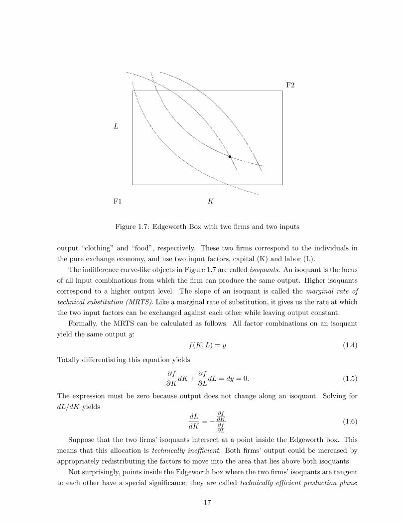
Figure 1.7: Edgeworth Box with two firms and two inputs

output “clothing” and “food”, respectively. These two firms correspond to the individuals in

the pure exchange economy, and use two input factors, capital (K) and labor (L).

The indifference curve-like objects in Figure 1.7 are called isoquants. An isoquant is the locus

of all input combinations from which the firm can produce the same output. Higher isoquants

correspond to a higher output level. The slope of an isoquant is called the marginal rate of

technical substitution (MRTS). Like a marginal rate of substitution, it gives us the rate at which

the two input factors can be exchanged against each other while leaving output constant.

Formally, the MRTS can be calculated as follows. All factor combinations on an isoquant

yield the same output y:

f(K,L) = y (1.4)

Totally differentiating this equation yields

∂f

∂KdK +

∂f

∂LdL = dy = 0. (1.5)

The expression must be zero because output does not change along an isoquant. Solving for

dL/dK yields

dL

dK= −

∂f∂K∂f∂L

(1.6)

Suppose that the two firms’ isoquants intersect at a point inside the Edgeworth box. This

means that this allocation is technically inefficient: Both firms’ output could be increased by

appropriately redistributing the factors to move into the area that lies above both isoquants.

Not surprisingly, points inside the Edgeworth box where the two firms’ isoquants are tangent

to each other have a special significance; they are called technically efficient production plans:

17

These distributions of the two inputs to both firms have the property that it is not possible to

increase one firm’s production without decreasing the other firm’s production.

The analogue to the utility possibility frontier in the pure exchange economy is called the

production possibility frontier in Figure 1.8 (also occasionally called the “transformation curve”).

The production possibility curve gives the maximal production level of one good, given the

production level of the other good. Points above the transformation curve are unattainable (not

feasible), while points below are inefficient, either because isoquants intersect, or because not

all inputs are used.

-

6

C

F

Figure 1.8: Production possibility curve

We are now interested in whether the result of the first theorem of welfare economics carries

over to an economy with production. Will a market economy achieve a technically efficient

allocation?

A profit maximizing firm’s objective is to produce its output in a cost-minimizing way.

minL,K

wL+ rK s.t.f(L,K) ≥ y, (1.7)

where w is the price of labor (wage) and r is the price of capital. Setting up the Lagrangean

and differentiating yields

w − λ∂f∂L

= 0 (1.8)

r − λ ∂f∂K

= 0 (1.9)

Bringing the second part of both equations on the right hand side on dividing through yields

w

r=

∂f∂L∂f∂K

(1.10)

18

Hence, a firm adjusts its MRTS to the negative of the factor price ratio. Since both firms face

the same factor price ratio, their MRTS will be the same. Hence, by the same reasoning that

implied that households’ MRSs are equalized in an exchange economy, we also find that a market

economy with cost minimizing firms achieves technical efficiency.

Each technically efficient allocation in the Edgeworth box corresponds to a point on the

production possibility frontier. While all points there are technically efficient, not all of them

are equally desirable. This is easy to see: Suppose we put all capital and all labor into clothing

production; this is technically efficient, because there is no way to increase the food production

without lowering the clothing production. Still, the product mix is evidently inefficient: People

in this economy would then be quite fashionable, but also very hungry! We need to satisfy a

third condition that guarantees an optimal product mix.

The slope of the production possibility curve is called the marginal rate of transformation

(MRT). The MRT tells us how many units of food the society has to give up in order to produce

one more unit of clothing. Note that “transformation” takes place here through reallocation of

labor and capital from food production into clothing production.

Formally, we can derive the MRT as follows. Suppose that we re-allocate some capital (dK)

from food into clothing production. This will change the production levels as follows:

dF =∂fF∂K

(−dK) (1.11)

dC =∂fC∂K

dK (1.12)

Dividing through each other, we have

dF

dC= −

∂fF∂K∂fC∂K

(1.13)

It is useful to relate the expression on the right hand side to the marginal cost of food and

clothing. Suppose we want to produce an extra unit of food; how much extra capital do we need

for this? Since dF = ∂fF∂K dK in this case, and we want dF to be equal to 1, we can solve for

dK = 1∂fF∂K

. The cost associated with this is hence

MCF =r∂fF∂K

(1.14)

Similarly,

MCC =r∂fC∂K

(1.15)

Hence, we can write (1.13) asdF

dC= −MCC

MCF(1.16)

19

What is the condition for an optimal product mix? Suppose that, say, MRTcf = dFdC = 2 >

1 = MRSAcf . This means that, if we give up one unit of clothing, we can produce two additional

units of food. Since A is willing to give up a unit of clothing in exchange for only one extra unit

of food, it is possible to make A better off without affecting B, so the initial allocation must

have been Pareto inefficient. More generally, whenever the MRT is not equal to the MRS, such

a rearrangement of resources is feasible and hence the optimal product mix condition is

MRT = MRS (1.17)

Note that it does not matter whose MRS is taken, because all individuals have the same MRS

in a market equilibrium.

We now want to show that a competitive market economy achieves an optimal product mix:

From the pure exchange economy analyzed above, we know that the household adapts optimally

such that MRScf = − pcpf

. On the producers’ side, the clothing firm maximizes its profit

pcC − CC(C), (1.18)

where CC(·) is the clothing firm’s cost function (sorry for the double usage of “C”for cost and

clothing). Taking the derivative with respect to output C yields the first order condition

pc − C ′C = 0 (1.19)

which we can rewrite as

MCCloth = pc : (1.20)

The optimal quantity for a competitive firm is at an output level where its marginal cost equals

the output price.

Similarly, profit maximization of the food firm implies

MCFood = pf (1.21)

Dividing these two equations through each other and multiplying with −1 therefore implies that

−MCClothMCFood

= MRTcf = − pcpf.

This is exactly the same expression as the = MRScf of households, so that a market economy

achieves an optimal product mix.

1.6 Application: Emissions reduction

Market prices have the very feature that they reflect the underlying scarcity ratios in the economy

and help to allocate resources into those of the different uses in which they are most valuable.

20

For example, when there is an excess demand for clothing, the (relative) price of clothing will

rise and, as a consequence, additional employment of factors like capital and labor into clothing

production becomes more attractive for entrepreneurs.

In this application, we will see how market mechanisms that lead to efficient resource al-

location can be used when we want to reduce environmental pollution in a cost efficient way.

Consider the case of SO2 (sulphur dioxide), one of the main ingredients of “acid rain”. SO2 is

produced as an unwanted by-product of many industrial production processes and emitted into

the environment. There are however different technologies that allow to filter out some of the

SO2. Some of these technologies are quite cheap, but do not reduce the SO2 by a lot, and others

are very effective, but cost a lot. Moreover, SO2 is produced in many different places, and some

technologies are more efficiently used in some lines of production than in others.

Suppose that we want to reduce the SO2 pollution by a certain amount The task to find

the way to reduce pollution that is (on aggregate) the least costly is quite a complex problem

that requires that the social planner (i.e., the government) knows the reduction cost function

for each firm.

Suppose that we want to reduce the overall level of pollution that arises from a variety of

sources by some fixed amount. Specifically, we assume that there are two firms that emit 1000

tons of SO2 each. We want to reduce pollution by 200 tons. If firm 1 reduces its emissions by

x1, it incurs a cost of

C1(x1) = 10x1 +x2110. (1.22)

Similarly, when firm 2 reduces its emissions by x2, it incurs a cost of

C2(x2) = 20x2 +x2210. (1.23)

We first calculate which reduction allocation minimizes total social cost of pollution reduction.

The minimization problem is

minx1,x2

10x1 +x2110

+ 20x2 +x2210

s.t. x1 + x2 = 200. (1.24)

The Lagrange function is

10x1 +x2110

+ 20x2 +x2210

+ λ[200− x1 − x2]. (1.25)

The first order conditions are

10 +x15− λ = 0 (1.26)

20 +x25− λ = 0 (1.27)

Solving both equations for λ and setting them equal gives 10+ x15 = 20+ x2

5 , hence x1 = 50+x2.

Together with the constraint x1 + x2 = 200, this yields the solution of

x1 = 125, x2 = 75. (1.28)

21

Hence, firm 1 should reduce its pollution by 125 tons, and firm 2 by 75 tons. The reason why

firm 1 should reduce its pollution by more than firm 2 is that the marginal costs of reduction

would be lower in firm 1 than in firm 2, if both firms reduced by the same amount; but such

a situation cannot be optimal, since one could decrease x2 and increase x1, and so reduce the

total cost.

Substituting the solution into the objective function shows that the minimal social cost to

reduce pollution by 200 tons is $ 4875.

For later reference, it is also helpful to note that

λ = 35. (1.29)

The Lagrange multiplier measures the marginal effect of changing the constant in the constraint.

Hence, λ = 35 means that the additional cost that we incur if we tighten the constraint by one

unit (i.e., if we increase the reduction amount from 200 to 201) is $35.

Figure 1.9 helps to understand the social optimum. The horizontal axis measures the 200

units of pollution that firm 1 and 2 must decrease their pollution in aggregate. The increasing

line is the marginal cost of pollution reduction for firm 1, MC1 = 10 + x15 . The second firm’s

marginal cost is MC2 = 20 + x25 , and since x2 = 200− x1 (by the requirement that both firms

together reduce by 200 units), this can be written as MC2 = 20 + 200−x15 = 60− x1

5 . This is the

decreasing line in Figure 1.9.

The social optimum is located at the point where the two marginal cost curves intersect,

at x1 = 125 (and, correspondingly, x2 = 75). Note that, for any allocation of the 200 units of

pollution reduction between the two firms (measured by the dividing point between x1 and the

rest of the 200 units), the total cost can be measured as the area below the MC1 curve up to the

dividing point, plus the area below MC2 from the dividing point on. It is clear that the total

area is minimized when the dividing point corresponds to the point where the two marginal cost

curves intersect. Any other allocation leads to higher total social costs. For example, if we asked

each firm to reduce its pollution by 100 units each, the additional costs (relative to the social

optimum) would be measured by the triangle ABC.

We can now turn to some other possible ways to achieve a 200 ton reduction. The first one

could be described as a command-and-control solution: The state picks some target level for

each firm, and the firms have to reduce their pollution by the required amount. In the example,

we want to reduce total pollution by 10% from the previous level, and therefore a “natural”

control solution is to require each firm to reduce its pollution by 10%, i.e. 100 tons. The total

cost of this allocation of pollution reduction is

10 · 100 +1002

10+ 20 · 100 +

1002

10= 5000, (1.30)

which is of course more than the minimal cost of 4875 calculated above.

22

6 6

125

A

100

B

C

``````````````````````````````````````

Figure 1.9: Efficient pollution reduction

Of course, we could in principle also implement the socially optimal solution as a command-

and-control solution. However, in practice, this requires that the state has information about the

reduction cost functions such that it can calculate the optimal solution. In practice, this extreme

amount of knowledge about all different firms is highly unlikely to be available to the state; the

following two solutions have the advantage that they rely on decentralized implementation: All

that is required is that each firm knows its own reduction cost.

The first solution is called a Pigou tax. Suppose that we charge each firm a tax t for each

unit of pollution that they emit. When choosing how many units of pollution to avoid, firm 1

then minimizes the cost of reduction minus the tax savings from lower emissions:

min 10x1 +x2110− tx1 (1.31)

23

Taking the derivative yields as first order condition:

10− t+x15

= 0, (1.32)

hence x1 = 5t − 50. The higher we set t, the more units of pollution will firm 1 reduce. Note

however that, if t < 10, the firm will not reduce any units, because the lowest marginal cost of

doing so (10) is higher than the benefit of doing so, t.

To which amount should we set t? From above, we know that the marginal cost of reduction

in the social optimal is $ 35, and indeed, if we set t = 35, we get x1 = 125, just like in the social

optimum.

Let us now consider firm 2. It minimizes

min 20x2 +x2210− tx1 (1.33)

Taking the derivative yields as first order condition:

20− t+x25

= 0, (1.34)

hence x2 = 5t− 100. Substituting t = 35 yields x2 = 75, again as in the social optimum. Hence,

we have shown that, if the state charges a Pigou tax of $35 per unit of SO2 emitted, firms will

reduce their pollution by 200 tons, and also do this in the most cost-efficient way.

Note that the cost of the Pigou tax for the two firms is substantial. Firm 1 has to pay

$35 for 875 tons, which is $ 30675. In addition to this, they have to pay abatement costs of

10 ·125+ 1252

10 = 2812.50. This is much more than firm 1’s burden under a command-and-control

solution, even if that is inefficient. This is the reason why firms are usually much more in favor

of command-and-control solutions to the pollution problem.

A third possible solution is called tradeable permits. Under this concept, each firm receives

a number of “pollution rights”. Each firm needs a permit per ton of SO2 that it emits, and a

firm that wants to pollute more than its initial endowment has to buy the additional permits

from the other firm, while a firm that avoids more can sell the permits that it does not need to

the other firm.

Suppose, for example, that both firms receive an endowment of 900 permits. Let p be the

market price at which permits are traded. If firm 1 reduces its pollution by x1 units, it can sell

x1 − 100 permits; if x1 − 100 < 0, then firm 1 would have to buy so many additional permits.

Firm 1 will maximize its revenue from permits minus its abatement costs:

p(x1 − 100)− 10x1 −x2110. (1.35)

The first order condition is

p− 10− x15

= 0, (1.36)

24

hence

x1 = 5p− 50. (1.37)

Similarly, firm 2 maximizes its revenue from permits minus its abatement costs:

p(x2 − 100)− 20x1 −x2210. (1.38)

The first order condition is

p− 20− x25

= 0, (1.39)

hence

x2 = 5p− 100. (1.40)

In total, the two firms have only 1800 permits, so that they need to avoid 200 tons of SO2.

Therefore,

5p− 50 + 5p− 100 = 200. (1.41)

Hence, the equilibrium price must be p = 35, and thus x1 = 125 and x2 = 75, just as in the

social optimum.

1.7 Second theorem of welfare economics

The second theorem of welfare economics states that (under certain conditions) every Pareto

optimum can be supported as a market equilibrium with positive prices for all goods. Hence,

together with the first theorem of welfare economics, the second theorem shows that there is a

one-to-one relation between market equilibria and Pareto optima.

In Figure 1.10, the Pareto optimum P can be implemented by redistributing from the initial

endowment E to R, and then letting the market operate in which A and B exchange goods so

as to move from R to P .

What is the practical implication of the second theorem? Suppose that the government

wants to redistribute, because the market outcome would lead to some people being very rich

(B in our example), while others are very poor (like A in the example). Still, one good property

of market equilibria is that they lead to a Pareto efficient allocation, and it would be nice to keep

this property even if the state interferes in the distribution. Of course, if the government knew

exactly the preferences of all individuals, it could just pick a Pareto optimum and redistribute

the goods accordingly. However, in practice this would be very difficult to achieve. A solution

suggested by the second theorem of welfare economics is that the government redistribution of

endowments does not have to go to a Pareto optimum directly, but can bring us to a point like

R, and starting from this point, individuals can start the market exchange of goods, which will

eventually bring us to P .

25

A

B

C

F

• R�P

•E�

Figure 1.10: Second theorem of welfare economics

1.8 Application: Subsidizing bread to help the poor?

Many developing countries choose to subsidize bread (or other basic foods) in an attempt to help

the poor. In the previous section on the second theorem of welfare economics, we have already

indicated that this might not be the most efficient way to implement this social assistance. The

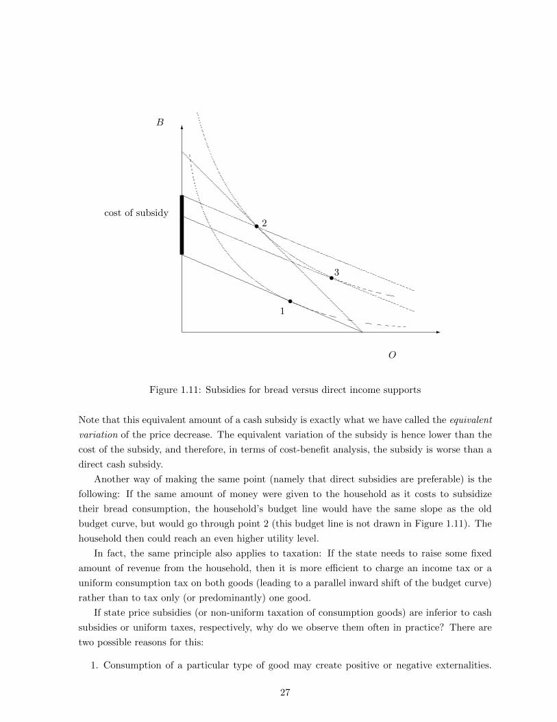
following Figure 1.11 helps us to analyze the situation.

In the initial situation without a subsidy, the household faces the lowest budget set and will

choose point 1 as the utility-maximizing consumption bundle. A subsidy of the bread price

implies that the household can now afford a larger quantity of bread for a given consumption

of other goods (but the maximum affordable quantity of other goods stays constant). In the

graph, the budget line turns in a clockwise direction around the point on the O-axis. The utility

maximizing bundle is now at point 2.

How much does the subsidy cost? For a given level of O, the dark line on the B-axis gives

the additional units of bread that the household can buy. Hence, the dark line measures the

cost of the subsidy in units of bread. (We can also measure the cost of the subsidy in units of

the other good, on the O-axis, between the point on the old budget curve and the budget line

parallel to it that goes through point 2).

There are, of course, other ways to increase the household’s utility than just to decrease the

bread price. If we don’t change prices, but rather give money directly, the old budget curve shifts

out in a parallel way. Once we reach the budget curve that is tangent to the higher indifference

curve at point 3, the household will be able to achieve the same utility level as with lower prices.

The cost of such a subsidy is lower than the cost of the bread subsidy; in units of bread, it is

the distance between the old budget line and the budget line through point 3, on the B-axis.

26

-

6

O

B

•1

• 2

•3

cost of subsidy

Figure 1.11: Subsidies for bread versus direct income supports

Note that this equivalent amount of a cash subsidy is exactly what we have called the equivalent

variation of the price decrease. The equivalent variation of the subsidy is hence lower than the

cost of the subsidy, and therefore, in terms of cost-benefit analysis, the subsidy is worse than a

direct cash subsidy.

Another way of making the same point (namely that direct subsidies are preferable) is the

following: If the same amount of money were given to the household as it costs to subsidize

their bread consumption, the household’s budget line would have the same slope as the old

budget curve, but would go through point 2 (this budget line is not drawn in Figure 1.11). The

household then could reach an even higher utility level.

In fact, the same principle also applies to taxation: If the state needs to raise some fixed

amount of revenue from the household, then it is more efficient to charge an income tax or a

uniform consumption tax on both goods (leading to a parallel inward shift of the budget curve)

rather than to tax only (or predominantly) one good.

If state price subsidies (or non-uniform taxation of consumption goods) are inferior to cash

subsidies or uniform taxes, respectively, why do we observe them often in practice? There are

two possible reasons for this:

1. Consumption of a particular type of good may create positive or negative externalities.

27

This means that other people (or firms) in the economy benefit or suffer, respectively,

from another consumer’s consumption. As examples, think of driving a car for a negative

externality (pollutes the environment, possibly creates traffic congestion) and getting a

vaccination against a contagious disease for a positive externality (if you don’t get ill, you

will also not pass the illness to other people). Naturally, each consumer will only take

his own utility into account when deciding whether and how much to consume each good.

Subsidies and taxes can be a tool to make people “internalize” the positive or negative

externalities that they impose on other people. We will cover this case in much more detail

in Chapter 4.

2. Redistributive subsidies (like the bread subsidy discussed above) may be justified if ad-

ministrative problems prevent direct cash subsidies. Suppose, for example, that a country

does not have a well-developed administration. If the state has not registered its citizens,

then there is no possibility to prevent people from collecting a cash subsidy multiple times

and so such a policy would be very expensive for the state. A bread subsidy, on the other

hand, can even be implemented if the beneficiaries are unknown.

In some sense, the problem with bread subsidies analyzed above has also to do with

“collecting the subsidy multiple times” (as people increase their bread consumption in

response to the subsidy). With a perfect administration system, collecting the cash subsidy

multiple times can be prevented, and the cash subsidy is preferable to a price subsidy

that would lead to a (non-preventable) consumption increase of the subsidized good. In

contrast, with a bad administration system, it might be much easier to collect a cash

subsidy multiple times than to increase the bread consumption, because there is a limit of

how much bread one can reasonably consume.

1.9 Limitations of efficiency results

Often, the efficiency result of the first theorem of welfare economics is interpreted by (conserva-

tive) politicians in the sense that the state should not interfere with the “natural” working of

the market, but rather keep both taxes and regulations to a minimum so as to not interfere with

the efficient market outcome. For example, when President Bush stated in the 2006 State of the

Union address that “America is addicted to oil” and suggested that new technologies should be

developed that allow for a higher domestic production of fuel, he also rejected the notion that

this development should be fostered by levying higher gas taxes, because this would “interfere

with the free market”.

While keeping the government small and taxes low is a perfectly defensible political preference

(as is the opposite point of view), it is hard to argue that this is a scientific consequence of

economics in general and the first welfare theorem in particular. In this section, we will briefly

talk about the real-world and theoretical limitations of the efficiency results.

28

1.9.1 Redistribution

The first class of limitation arguments applies even within the simple exchange model that we

used to derive the first theorem of welfare economics and notes that, while efficiency is a desirable

property of allocations, but it is not the only criterion on which people want to judge whether

a certain allocation of resources is “good”.

If the initial distribution of goods is very unequal (perhaps because some agents have in-

herited a fortune from their ancestors, while others did not inherit anything), then the market

outcome, while being Pareto better than the initial endowment and also a Pareto optimum, is

also highly unequal. Therefore, while this allocation is efficient, it may not be what we consider

“fair”. Moreover, there are many other Pareto optima that could be reached by redistributing

some of the initial endowments. Hence, the desire that the economy achieves a Pareto efficient

allocation does not, in theory, provide an argument against any redistributive tax.

In practice, redistributive taxes may lead to some distortions that reduce efficiency. The

reason is that it is very difficult in practice to tax “endowments” that arise without any action

taken by the individual. The inheritance tax is probably closest to the ideal of an endowment

taxation, but many other taxes are not. For example, when taxing income, the state does not

impound a part of the “labor endowment” of an individual, but rather lets the individual choose

how much to work and how much money to earn and then levies a percentage of the income as

tax. While this appears to be the only practical way in which we can tax income, it is also more

problematic than an endowment tax since individuals may choose to work less than they would

without taxation, as a lower gross income also reduces the amount of taxes that they have to

pay, and this effect leads to an inefficiency.3

1.9.2 Market failure

The second class of arguments that limit the efficiency result has to do with the fact that the

model in which the result was derived is based on a number of assumptions that need not be

satisfied in the real world. Consequently, in more realistic models, a market economy may not

achieve a Pareto optimum. This phenomenon is called market failure and will be the subject of

the next chapters.

In particular, in the simple Edgeworth model, we assume that all consumers and firms behave

competitively. In Chapter 2, we analyze what happens in markets that are less competitive.

Second, all goods in the Edgeworth box model are what is called private goods: If one

consumer consumes a unit of a private good, the same unit cannot be consumed by any other

consumer and consequently their utility is unaffected by the behavior of other consumers. In

Chapters 3 and 4, we will see that there are some goods for which this is not true. For example,

3A more detailed analysis of the welfare effects of labor taxation is beyond the scope of this course and covered

in the taxation course.

29

all people in a country “consume” the same quality of “national defense” (the protection afforded

against invasions by other countries). National defense is therefore what is called a public good.

If public goods were provided individually by private agents, there would likely be a level of

provision that is smaller than the efficient level, because each private individual that contributes

to the public good would primarily consider his own cost and benefits from the public good, but

neglect the benefits that accrue from his provision to other individuals. A similar phenomenon

occurs when people do not only care about their own consumption, but are also affected by

other people’s consumption. For example, if a firm pollutes the environment as a by-product of

its production, other consumers or firms may be negatively affected. Such negative externalities

that are not considered by the decision maker lead to the result that, in the market equilibrium,

too much of the activity that generates the negative externality would be undertaken. There

are also positive externalities that are very similar in their effects to public goods, and again,

the market equilibrium may not provide the efficient allocation.

Finally, the quality of the goods traded are known to all parties in the Edgeworth box model.

In Chapter 5, we analyze which problems arise when one agent knows some information that

is relevant for the trade, while his potential trading partner does not have that information

(but knows that the other one has some informational advantage over him). This phenomenon

is very relevant in insurance markets where individuals may be much better informed than

insurers as to how likely they are to experience a loss, or how careful they are in avoiding a loss.

In markets where these effects are particularly important, the uninformed party is reluctant to

be taken advantage of by a counterpart that has very negative information; for example, the

sickest persons would be much more likely to buy a lot of health insurance than those persons

who feel that they are likely to remain healthy during the insured period. Therefore, (private)

insurance companies might expect to face a worse-than-average distribution of potential clients,

which forces them to increase prices, which again makes insurance even less attractive for low

risk individuals. This spiral may lead to the result that health insurance is not provided at all

in a market equilibrium, or only at a very high cost and for the least healthy people.

Whenever market failure is a problem, there usually exists a policy that allows the state to

intervene in the market through regulation, public provision or taxation in a way that increases

social welfare. In each of the following chapters, we will derive this optimal intervention.

1.10 Utility theory and the measurement of benefits

In reality, there are very few policy measures that lead to Pareto improvements (or deterio-

rations). As a consequence, a state cannot use the Pareto criterion for the question whether

a particular policy measure should be implemented or not. Comparing costs and benefits is

particularly difficult if they do not come in lump-sums for all individuals, but rather the project

influences the prices in the economy. “Prices” should be interpreted in a very broad sense here;

30

for example, if the state builds a bridge that reduces the travel time between cities A and B,

then it decreases the (effective) price for traveling between A and B (this is true even if, or

actually, in particular if, the state does not charge for the usage of the new bridge). In this

section, we develop a theoretical approach to comparing the benefits of winners with the cost of

losers. However, to do this, we need to first refresh some facts from microeconomic theory.

1.10.1 Utility maximization and preferences

I assume that you have already taken a course in microeconomics, so the content of this section

should just be a quick refresher. If you feel that you need a more thorough review, I recommend

that you go back to your microeconomics textbook.

The household in microeconomics is assumed to have a utility function that it maximizes

by choosing which bundle of goods to consume, subject to a budget constraint that limits the

bundles it can afford to buy. This utility function is, from a formal point of view, very similar

to the production function of a firm. However, there is an important difference: The production

function is a relatively obvious concept, as inputs are (physically) transformed into outputs, and

both inputs and outputs can be measured.

It is less obvious that the consumption of goods produces “joy” or happiness for the household

in a similar way, because there is no way how we can measure a household’s level of happiness.

While the household probably can say that it likes one situation better than another one, it is

hard to tell “by how much”. Moreover, we know from introspection that we do not go to the

supermarket and maximize explicitly a particular utility function through our purchases.

It is therefore clear that a utility function is perhaps a useful mathematical concept, but one

for which the foundations need to be clarified. The first step is therefore to show which primitive

assumptions lead us to conclude that a consumer behaves as if he maximized a utility function.

This is what we will turn to next.

(Preference) rankings

Each consumer is assumed to have a preference ranking over the available consumption bundles:

This means that the consumer can compare alternative consumption bundles4 (say, x and y)

and can say whether x is at least as good as y (denoted x � y, or y is at least as good as x, or

both. If both x is at least as good as y and y is at least as good as x, we say that the individual

is indifferent between x and y, and write x ∼ y.

The preference relation is an example of a more general mathematical concept called a

relation, which is basically a comparison between pairs of two elements in a given set. Before

we turn to the preference relation in more detail, here are three other examples of a relation:

4Remember that a consumption bundle in an economy with n different goods is a n-dimensional vector; the

ith entry in this vector tells us the quantity of good i in the bundle. For example, in a two-good (say, apples and

bananas) economy, the bundle (1, 4) means that the individual gets to consume 1 apple and 4 bananas.

31

1. The relation R1 =“is at least as old as”, defined on a set of people.

2. The relation R2 =“is at least as old as and at least as tall as”, defined on a set of people.

3. The relation R3 =“is preferred by a majority of voters to”, defined on a set of different

political candidates (and for a given set of voters)

Some relations have special properties. For example, the relation R1 is complete, in the sense

that, for any set of people and any pair (x, y) from that set, we can determine whether “x is at

least as old as y” or “y is at least as old as x” (or perhaps both, if they have the same age).

Not every relation is complete; for example, R2 is not: There could be two people, say Abe

and Beth such that Beth is older than Abe, but Abe is taller than Beth. In this case, we have

neither “Abe is at least as old as and at least as tall as Beth” nor “Beth is at least as old as and

at least as tall as Abe”.

Another property is called transitivity and has to do with comparison “chains” of three

elements. For example, consider relation R1: If we know that “Beth is at least as old as Abe”

and “Clarence is at least as old as Beth”, we know that it must be true “Clarence is at least

as old as Abe”. Since the relation “goes over” from the first two comparisons to the third,

relation R1 is called “transitive”. You can check that R2 is also transitive, but we will see later

in Chapter 6 that the relation R3 is not transitive, as it is possible to construct a society of

voters with preference such that a majority of voters prefers Abe to Beth and Beth to Clarence,

but Clarence to Abe.

Now, what special properties are reasonable to require from the “is at least as good as”

preference relation, which is the basis for household theory? The following are three standard

assumptions on preferences:

1. Complete: For all x and y, either x � y or y � x or both.

2. Reflexive: For all x, x � x. (This is a very obvious and technical assumption).

3. Transitive: If x � y and y � z, then x � z.

As above, completeness means that the individual can compare all pairs of bundles of goods and

find either one of the bundles better than the other on, or is indifferent between them. In other

words, there is never a situation in which the individual “does not know” which one is better

for him. Reflexivity is a more technical assumption that essentially says that the individual

is indifferent between two equal bundles.5 Transitivity requires that, if the individual prefers

x to y, and prefers y to z, then he should also prefer x to z. Transitivity is a very natural

requirement for individual preferences over goods.

We usually make two additional regularity assumptions:

5Can you think of an example of another relation that is not reflexive?

32

4. Continuity: For all y, the sets {x � y} and {x � y} are closed sets.

5. Monotonicity: If x ≥ y and x 6= y, then x � y.

Continuity is a technical assumption that is needed in the proof of the existence of a utility

function. Monotonicity just says that if x contains more units in each category (more vegetables,

more cars, more clothes etc.), then the individual prefers bundle x.

Utility functions

We will now link preferences to the concept of a utility function. We say that a utility function

u represents the preferences � if

u(x) ≥ u(y) ⇐⇒ x � y.

That is, whenever the individual feels that x is at least as good as y, the “utility” value that

the utility function returns when we plug in x is at least as large as the utility value that y

returns. In other words, we know from the utility function which of two bundles an individual

prefers, and so knowing the utility function gives you complete information about an individual’s

preferences.

We can now state one of the main results from household theory, namely that there exists a

utility function that represents the preferences.

Proposition 2. If the preference ordering is complete, reflexive, transitive, continuous and

monotone, then there exists a continuous utility function Rk → R which represents those pref-

erences.

Proof. Let e = (1, 1, . . . , 1) ∈ Rk. Consider the following candidate for a utility function:

x ∼ u(x)e. That is, we look for the bundle that is located on the 45 degree line and makes the

individual indifferent to x. This equivalent bundle on the 45 degree line is some multiple of e

(for example, the equivalent bundle is (5, 5, . . . , 5)), and we call the multiple the “utility” of x;

in the example, the utility of x would be 5.

We now have to prove that such a function u(·) exists and “works” as a utility function.

The first step is to show that u(x) exists and is unique. First, note that the set of bundles that

are at least as good as x and the set of bundles that are not better than x are nonempty. By

the assumption of continuity of preferences, there exists one value u such that ue ∼ x, and we

call it u(x). (Moreover, it is clear that there is only one such value, otherwise we would get a

contradiction to the assumption of monotonicity.)

We now show that the function that we have constructed this way is a utility function,

that is, if x � y, then u(x) ≥ u(y) and vice versa. Suppose we start with a pair of x and y

such that x � y. We construct equivalent bundles to x and y, which therefore must satisfy

u(x)e ∼ x � y ∼ u(y)e, and hence u(x)e � u(y)e. These are two bundles that both lie on

33

the 45 degree line, so one of them must be component-wise larger (or, more exactly “no smaller

than”) the other one. Specifically, monotonicity implies that u(x) ≥ u(y), so that we have

shown that, if x � y, then u(x) ≥ u(y). A similar argument holds for the reverse direction.

Note that the choice of the unit vector e = (1, 1) in the above proof was arbitrary, and

other base vectors will lead to different numerical utility values. Moreover, any increasing

transformation of a utility function represents exactly the same preferences.

This implies that observation can never reveal the “true” utility function of an individual,

because there are very many functions that represent an individual’s preferences. For example,

if u(·) is a utility function that represents an individual’s preferences, then v(x) = 15 + u(x)/2

also represents the same preferences. Therefore, differences in utility levels between different

situation do not have a concrete meaning. We say that the utility function is an ordinal, not a

cardinal concept. “Ordinal” means that the utility values of different bundles only indicate the

ordinal ranking (i.e., if u(x) = 12 and u(y) = 3, we can say that x � y, but saying that “x

is four times as good as y does not make sense). In contrast, a cardinal measure is one where

differences and relations have meaning (as in “$12 is four times as much as $3”).

The fact that utility functions are an ordinal concept also implies that an inter-personal

comparison of utilities does not have a useful interpretation. For example, we cannot find out

whether a social project that increases the utility of some people and decreases that of others

is “socially beneficial” by adding the utility values of all people in both situations (before and

after) and just comparing the utility sum. We need some other measure of utility changes that

can be compared across individuals, and this is the subject of the next section.

1.10.2 Cost-benefit analysis

How can we decide whether a policy measure that benefits some individuals and harms others

is “overall worth it”? We need a measure that converts the utility gains and losses into money

equivalents.

Consider the following example. The state has the possibility to build a dam with a hydro-

electric power plant. If built, the prices will decrease from p0 to p1.6 Suppose that the set of

people who benefit from the lower prices is not necessarily the same as those who have to finance

the construction, so some will be better off, some worse off. We therefore need a measure of

“how much” those people who benefit from lower electricity prices are better off. The relevant

concepts from household theory are called the equivalent and the compensating variation, but

before we can define them we will need to review some household theory.

6As above with x and y, bold-faced letters indicate vectors of prices. Furthermore, p1 ≤ p0 means that some

(at least one) prices are strictly lower at time 1 than at time 0, and that no good’s price is higher at time 1 than

at time 0.

34

A brief review of household theory

The utility maximization problem of the household is also called the “primal problem”:

maxu(x) s.t. M − px = 0. (1.42)

That is, the household chooses the optimal bundle of goods x to consume, subject to the con-

straint that total expenditures px cannot be larger than income M . The solution of this problem

is a function x = (x1, x2, . . .) that depends on the exogenous parameters of the problem, that is

here the income M and the prices p. The solution is called the Marshallian demand function

x(p,M). It tells us how much of each good the household optimally consumes, at prices p and

income M .

The value function, which results from plugging the Marshallian demand functions back into

the objective function (i.e., into the utility function u(x)), is called the indirect utility function

v(p,M). It tells us the maximum utility that the individual can achieve for given prices p and

income M .

Alternatively, the household can also be thought of as solving an expenditure minimization

problem, subject to the constraint that some minimum utility level is reached. This problem is

called the “dual” problem. Formally, it results when we interchange the roles of the objective

and the constraint in the primal (utility maximization) problem:

minx

px s.t. u(x) ≥ u (1.43)

How are the solutions and parameters for the primal and dual problem related to each other?

Suppose that x∗ is the solution of the primal problem for income M∗ and prices p; let the

value of the objective function, u(x∗), be denoted by u∗. If we take u∗ and set the value of the

constraint in the dual problem to u = u∗, then the solution of the dual problem is exactly the

same x∗ as in the original problem and the value of the dual objective function is M∗.7 This

relation between the primal and the dual problem is known as duality.

The solution of the dual problem is again a value for all xi, but now depending on the

parameters of the expenditure minimization problem, which are prices p and the exogenous

target utility u. The solution is called the Hicksian (or compensated) demand function H(p, u).

The value function of the dual problem results when we substitute the Hicksian demand

functions into the objective function px. The resulting function e(p, u) = pH(p, u) is called

the expenditure function. It tells us the minimum income that is necessary for the individual to

achieve utility u at prices p.

7To see this, suppose x∗ is not a solution of the expenditure minimization problem, but rather there is a x′

which delivers utility u∗ at expenditures M ′ < M∗. Then there exists ε > 0 such that p(x′ + ε) = M∗ and

u(x′ + ε) > u(x′) = u(x∗), so x∗ cannot be the solution of the primal problem.

35

Compensating and equivalent variation

We now return to our original problem of measuring the benefit of a price decrease. Consider

an individual who benefits from the price decrease. At prices p0, he reaches a utility level of

u0, and at prices p1 a utility level of u1. Since prices decreased, p1 ≤ p0, the utility level has

increased: u1 > u0. The question is, how much is the utility increase worth in money, which

can be compared across people.

The equivalent variation answers the following question: If prices did not change (because

the project is not implemented), how much extra income would be necessary for the individual

to reach utility level u1? In other words, which increase in income, at the old prices, would be

equivalent to a reduction in electricity prices?

EV = e(p0, u1)− e(p0, u0) = e(p0, u1)−M, (1.44)

where M is the income of the individual, assumed to be equal at time t = 0 and t = 1. (That

e(p0, u0) = M is a consequence of our initial definition that at prices p0 and income M , the

individual could reach utility level u0; hence M must be the minimum expenditure to reach

utility level u0 at prices p0.) Note that the question answered by the EV is relevant, if there is

some amount of money available that is either spent on the project or distributed to households

(for example, by tax reductions).

The compensating variation answers the following question: “After the price change has

taken place, how much money could be taken away from the individual so that he is still at least

as well off as before the price change?” The term compensating comes from the fact that, when

the price change is an increase, the calculated amount is the increase in income that is necessary

to compensate the individual for the higher prices, that is, to keep his utility level constant.

CV = e(p1, u1)− e(p1, u0) = M − e(p1, u0). (1.45)

Again, M = e(p1, u1), since the individual can just reach utility level u1 at prices p1 and income

M , and so the minimum income to reach utility level u1 at prices p1, i.e. e(p1, u1), is M .

The question answered by the CV is relevant, if the amount required for the implementation

of the project has to be raised by taxes from the individuals. If the sum of the compensating

variations (over all individuals that benefit) is higher than the cost of the project, then the

project should be implemented.

Graphical analysis of CV and EV

In Figure 1.12, we analyze graphically the compensating and equivalent variation. Electricity E

in our example is measured on the vertical axis, while the good on the horizontal axis, O, can

either be thought of as a single other good, or as a composite of all other goods, whose price

is assumed to remain constant. Without loss of generality, we can assume that the price of the

other good is normalized to one.

36

-

6

O

E

•1

• 2

•3

EV

Figure 1.12: EV for electricity price change

Point 1 corresponds to the initial situation in which the household reaches the lower indif-

ference curve. When the price of electricity drops, the households budget curve pivots coun-

terclockwise around the intersection of the budget curve with the horizontal axis (because the

quantity of O that the household can consume, if it chooses not to buy any E, has not changed).

The optimal consumption for the household is to consume at point 2 on the higher indifference

curve.

The equivalent variation asks how much money we would have had to transfer to the house-

hold at the old prices so that the household could reach the same higher utility level. Note

that a transfer of money at the old prices just corresponds to a parallel outward shift of the

old budget curve; to reach the same utility level as with the price decrease, we have to shift

the budget curve until we reach the indifference curve at point 3. Graphically, the difference

between these two budget lines measured on the vertical axis (the bold part of the axis) is equal

to the equivalent variation measured in units of electricity. If we measure the difference between

the two budget lines instead along the horizontal axis, we get the equivalent variation measured

in units of the other good (and, if we normalize the price of this good to 1, then we get the EV

measured in money).

Now consider Figure 1.13 for the compensating variation. Again, the original situation, point

37

1 and the situation after the price change, point 2, are the same as in Figure 1.12. However,

now we ask how much money we can take away from the individual at the new prices such that

he still reaches at least the old utility level.

-

6

O

E

@@@@@@@@@@@@@@@

• 1

• 2

•3

CV

CV

Figure 1.13: CV for electricity price change

Graphically, that is: How much can we shift back the new (steeper) budget curve so that

we are again back to the initial utility level? We see that the initial utility level is reached at

point 3 and so the difference between the budget curve through point 2 and that through point 3

measures the compensating variation. As with the equivalent variation above, we can measure

that difference either vertically, along the E axis, in which case it is the CV measured in units

of E, or along the horizontal axis, in which case it is measured in units of O.

A numerical example

Consider the utility function u(x1, x2) = xa1x1−a2 . Let us first solve the primal problem. The

Lagrange function is

xa1x1−a2 + λ[M − p1x1 − p2x2]. (1.46)

38

Differentiating with respect x1 and x2 yields the first order conditions:

axa−11 x1−a2 − λp1 = 0 (1.47)

(1− a)xa1x−a2 − λp2 = 0 (1.48)

Bringing λp1 and λp2 on the other side and dividing both equations through each other yields

ax2(1− a)x1

=p1p2

(1.49)

and hence p1x1 = a1−ap2x2. Using this in the budget constraint yields

M =

[a

1− a+ 1

]p2x2 =

1

1− ap2x2, (1.50)

hence

x2 =(1− a)M

p2(1.51)

and using this in (1.49) yields

x1 =aM

p1(1.52)

When we substitute these solutions for x1 and x2 back in the objective function, we get the

indirect utility function

v(p1, p2,M) =

(aM

p1

)a((1− a)M

p2

)1−a= aa(1− a)1−a

M

pa1p1−a2

(1.53)

Let us now turn to the expenditure minimization problem

min p1x1 + p2x2 s.t. xa1x1−a2 ≥ u (1.54)

The Lagrange function is

p1x1 + p2x2 + λ[u− xa1x1−a2

](1.55)

The first order conditions are

p1 − λaxa−11 x1−a2 = 0 (1.56)

p2 − λ(1− a)xa1x−a2 = 0 (1.57)

Bringing p1 and p2 on the other side and dividing yields

p1p2

=a

1− ax2x1

(1.58)

and solving this for x1 yields

x1 =a

1− ap2p1x2 (1.59)

39

Using this expression to substitute for x1 in the constraint, and solving the constraint for x2

yields

x2 =

(1− aa

)a(p1p2

)au (1.60)

and

x1 =

(a

1− a

)1−a(p2p1

)1−au (1.61)

Substituting these solutions into the objective function yields the expenditure function

e(p1, p2, u) =

[(a

1− a

)1−a+

(1− aa

)a]pa1p

1−a2 u (1.62)

Let us now turn to calculating the compensating and equivalent variations. Assume that

a = 1/2. Suppose that the household has a income of 100, and the price of good 2 is normalized

to 1 in both cases. Before the dam is built, the price of electricity is p01 = 4, and if it is built, it

drops to p11 = 1.

By substituting in the indirect utility function, we find that

u0 =100

2√

1 · 4= 25 (1.63)

and

u1 =100

2√

1 · 1= 50 (1.64)

The compensating variation is

CV = M − e(1, 1, 25) = 50. (1.65)

This tells us that, at the new lower prices, we could tax the household up to $ 50, and the

household would still be no worse off than in the old, high-price situation.

The equivalent variation is

EV = e(4, 1, 50)−M = 100. (1.66)

This means that, if we don’t build the dam and hence the electricity price stays at $4, then

we would need $100 of additional income to make the household as well off as with the price

change.

1.11 Partial equilibrium measures of welfare

In section 1.10.2, we have calculated the benefits of price changes using a “general equilibrium

framework” in which the complete utility optimization problem of the household is solved. In

this section, we restrict the analysis to a partial equilibrium framework, in which we look at

40

-

6

q

p

@@@@@@@@@@@@@@@

D = MWP

Figure 1.14: Consumers’ demand function as marginal willingness to pay

only one market. Theoretically speaking, this approach is not completely exact, but for most

markets, it is a very useful and quite accurate approximation.

Consider the demand function in Figure 1.14. The dollar value at a particular quantity gives

the marginal willingness to pay for this unit of output. The area under the demand curve,

measured from 0 to the quantity sold, is therefore a measure of the total (gross) benefit created

by all units in this market. (“Gross” consumer surplus refers to the fact that the cost of purchase

needs to be deducted to get the “net” consumer surplus).

Consider now Figure 1.15. A firm’s profit as it depends on output x is

px− C(x), (1.67)

so that the optimal x satisfies

p− C ′(x) = 0. (1.68)

This expression implies that a firm’s supply curve S(p) is the inverse of its marginal cost function.

For any output level x, the supply curve gives the cost for the production of the last unit (i.e.,

unit x). The area under the supply curve between 0 and x is therefore the variable cost of

producing x units (i.e., the total cost, but excluding possible fixed cost).

In Figure 1.16, we combine demand and supply functions. The area between the supply and

the demand curve is therefore equal to the net social benefit generated by this market: It is the

gross social benefit minus the production cost. The market equilibrium quantity is exactly the

quantity that maximizes this net social benefit. Quantities that deviate to the left or the right

from the equilibrium quantity have a reduced net social surplus. Specifically, if the deviation is

to a lower quantity than corresponds to the intersection of supply and demand curve, then some

41

-

6

q

p

����

����

����

����

�� S = MC

Figure 1.15: Supply function as marginal cost functions

-

6

q

p

@@@@@@@@@@@@@@@

D����

����

����

����

�� S

Figure 1.16: Market equilibrium, consumer surplus and producer rent

units are not produced that would provide larger benefits than it costs to produce them. If the

deviation is to a higher quantity, then some units are produced that cause higher costs than the

benefits they provide for consumers.

42

1.12 Applications of partial welfare measures

1.12.1 Welfare effects of an excise tax

The following Figure 1.17 shows the welfare effect of an excise tax, that is, a tax that is levied

on a particular good. Examples are taxes on cigarettes or gasoline and usually are some fixed

amount per unit of the good sold.

-

6

x

p

@@@@@@@@@@@@@@@@@@

D����

����

����

����

�����

S

����

����

����

����

�����

S′

x0x1

p0

pB1

pS1

Figure 1.17: Example: The welfare effect of an excise tax

Without a tax, the market demand and supply functions are given by D and S, respectively,

resulting in a quantity x0 being traded at price p0. An excise tax of t per unit works exactly like

an increase of the marginal costs by t and therefore shifts the supply function up by t. In the new

equilibrium, x1 units are traded, and consumers have to pay pB1 for each unit. Since producers

have to pay t to the state for every unit that they sell, producers only receive pS1 = pB1 − t for

each unit.

Any excise tax will (at least weakly) increase the price that consumers have to pay and

decrease the price that firms receive (net of the tax). In the graph, the supply curve is relatively

more elastic (i.e., flatter) than the demand curve, which is quite inelastic. As a consequence, the

tax increases the price that consumers have to pay by more than it lowers the price that firms

receive. In general, the market side with the more inelastic curve has to bear a greater part of

the burden (as measured by the price change).

The quantity traded in this market decreases from the socially optimal value of x0 to x1.

Units between x1 and x0 would have created a social benefit equal to the area under the demand

43

curve, from x1 to x0; to produce these units, the social costs are equal to the area under the

(old) S-curve (which is still the curve that gives the social marginal cost of production). Hence,

the tax leads to a social welfare loss equal to the area of the triangle delineated by D, S and the

vertical line at x1.

1.12.2 Welfare effect of a subsidy

We next consider the welfare effect of a subsidy. In Figure 1.18, a subsidy, paid to the sellers of

the good, shifts the original supply curve downward. The new equilibrium is at the intersection

of the demand curve and the new, shifted, supply curve.

-

6

x

p

@@@@@@@@@@@@@@@

D

����

����

����

����

�� S

����

����

����

����

�� S′

x0 x1

p0pS1

pB1

Figure 1.18: Example: The welfare effect of a subsidy

From a social point of view, the production cost of the additional units is given by the area

under the supply curve, between x0 and x1. The additional gross benefit to consumers is given

by the area under the demand curve, between x0 and x1. Hence, the additional production cost

is higher than the benefit created, and thus the subsidy leads to a welfare loss of the triangle

enclosed by the demand, the old supply curve and the vertical line at x = x1.

1.12.3 Price ceiling

In this section, we analyze the effect of a price ceiling: A price ceiling is often introduced in times

of war or natural catastrophes; a price ceiling prohibits any trades between firms and consumers

at a price that is higher than the price ceiling p. The objective is to prevent the change in

demand and/or supply to lead to a sharp increase in price that would benefit the sellers of the

good, while harming the consumers.

44

Since an effective price ceiling p is below the equilibrium price in the market, the demand at

that price is higher than the equilibrium quantity, and the supply is smaller than the equilibrium

quantity. In such a situation, the “shorter” side of the market determines how many units of

the good are traded. Here, the quantity traded is hence the quantity that firms are willing to

supply at a price equal to the price ceiling.

-

6

x

p

@@@@@@@@@@@@@@@@@@@@

D

����

����

����

����

����

����

S

p

xDxS

Figure 1.19: Price ceilings

Clearly, there is a welfare loss in the form of the triangle formed by S, D and the line x = xS ,

because these units that would have created a higher social benefit than their cost of production,

are not produced.

There are two other problems associated with price ceilings. First, whenever there is a

binding price ceiling, there is unsatisfied demand that is willing to pay a higher price than the

price ceiling in order to consume the good. This creates the conditions that are necessary for

a black market to arise. However, when there is a black market, then firms will tend to be

unwilling to sell their product for the low regulated price on the regular market, and eventually,

this means that the shortage on the regular market increases and the price ceiling becomes

ineffective.

The second problem arises even without a black market. So far, we have assumed that

the excess demand is satisfied by “efficient rationing”; that is, the highest demand individuals

45

receive the goods that are being sold. Alternatively, there could be random rationing, so that

each customer who is willing to pay the price ceiling price has an equal chance of being selected

for the good. In this case, some high demand customers are be served, and are replaced by

customers with a lower willingness to pay. This also creates a deadweight loss equal to the

difference of their willingness to pay.

1.12.4 Agricultural subsidies and excess production

Many countries attempt to help their farmers by subsidizing the price of domestically produced

agricultural goods, while keeping foreign agricultural products out of the country through the

use of tariffs. In the U.S., this description applies, for example, to sugar and ethanol, both of

which are produced at considerably lower costs in Latin America than domestically. Figure 1.20

helps us to analyze this case.

-

6

x

p

@@@@@@@@@@@@@@@@@@@@

D

����

����

����

����

����

����

S

pW

pS

a

b

c d

e

f g

hij

k

xSxD

Figure 1.20: Agricultural subsidies and quotas

The price pW gives the world market price at which this country can buy as much as it wants.

The curve S is the marginal cost of domestic producers, and D is the demand curve. If no tariffs

are imposed and also no subsidies are paid, then the equilibrium is given by the intersection

of the demand curve with the world market price line (point d; note that the intersection of

the domestic S-curve and the D-curve, point k, does not have any special significance in this

46

scenario). The price is pW . The consumer surplus is the triangle bde. Only domestic farmers

whose marginal cost are below the world market price produce and make a profit given by the

triangle abc.

Now suppose that the state pays farmers a subsidized price of pS for each unit. Also, it

imposes an import tariff of pS − pW on foreign products, so that the domestic market price rises

to pS relative to the situation before. Demand decrease to xD, and consumer surplus decreases

by the area bdij.

Domestic farmers now produce xS , the quantity where the marginal cost equals the subsidized

price pS . The producer surplus grows by the area bchj.

Clearly, there is an excess supply of xS − xD that must be bought by the government. Since

there is no domestic demand for these goods (at the new price level), this excess production

must be sold on the world market, where we of course only get a price of pW per unit. Hence,

the state makes a loss of pS − pW on each of the xS − xD units, and thus the total cost of the

subsidy for the state is given by the rectangular area fghi.

Hence, the policy has the following welfare effect on the three groups involved. Producers

have a benefit of area bchj, consumers have a loss of area bdij, and the state has a cost of area

fghi. If we just compare producers and consumers and cancel out areas that are at the same

time gains for producers and losses for consumers, we get a welfare effect of ihk–cdk, which may

be positive of negative. However, since the area ihk is entirely contained in the cost-of-subsidy

area fghi, it follows that the subsidy policy leads to an overall welfare loss, once we also consider

the expenditures of the state.

1.13 Non-price-based allocation systems

Up to now, we have assumed that goods are allocated in markets, where sellers charge a monetary

price to buyers. This is the most important method of allocation for most private goods.

However, for some goods, other allocation methods are used. In this section, we want to briefly

analyze why this might be the case and what the advantages and disadvantages of the different

allocation methods are.

Generally speaking, the social purpose of an allocation system is to decide which of many

possible users gets to consume the good. For example, for the allocation system of “selling”, the

available units of the good are given to those people who are willing to pay the equilibrium price,

and the equilibrium buyers of the good will be those people who have the highest willingness to

pay for that good.

From a social point of view, this is usually desirable for “private” goods — we would not

want to re-allocate the goods to somebody else with a lower willingness to pay, as that would just

waste welfare. However, in some examples, we may have a different idea about who the “right”

people are (to whom we want to allocate the goods), and this may influence which allocation

47

system should be chosen.

To operate an allocation system, the initial owner of the goods and/or the potential buyers

must also often expend resources; some systems are cheaper to operate and this influences how

desirable a particular allocation system is from a social point of view.

We now consider five different allocation systems, with examples for when they are applied,

and describing advantages and disadvantages. We start with the standard allocation system in

economics, selling.

Selling. Suppose we have 10 units of a good, to be distributed among 20 people who are

interested in obtaining at most one unit each, but have different willingnesses to pay for that

unit. If the seller charges a price that lies between the 10th and the 11th highest willingness to

pay, then the 10 people who have the highest willingness to pay are willing to pay such a price,

while the remaining 10 potential customers are not.

Hence, the allocation system of selling allocates the goods to the people with the highest

willingness to pay for the good. In most cases (but not always), this is a very desirable property.

In terms of administering the allocation system (i.e., in terms of cost), selling usually requires

some intermediate resource cost. Giving away the good for free is usually cheaper (in terms of

the resources needed to distribute the good to the customers, and those resources expended by

the customers in the process), but most other systems are more expensive.

Queuing. Consider the same allocation problem as above, but now assume that the initial

owner announces he will distribute the 10 units for free, at some time from now, say, in two

weeks. The goods will go to the first 10 people who come to request one unit. (More generally,

the phenomenon of queuing arises whenever the sale price for the n units to be distributed is

below the willingness to pay of the n+ 1st person, thus generating excess demand.)

If the price were truly zero, there would be more people interested in the good than units

available. It is not an equilibrium that all of them queue up, though, because those who are the

last ones in the queue do not get a unit and therefore are better off going home. It is also not

an equilibrium that there is no queue because then, all individuals would try to get the good.

Hence, there will be an intermediate number of people queuing up in equilibrium. Precisely, in

equilibrium, exactly 10 people should queue up (the 11th person who comes to the queue would

know that no good will be available once he reaches the top of the line, and should therefore

not line up — of course, this argument requires that the number of items to be distributed is

known exactly).

In general, the length of time that people have to wait in a queue generates an additional

“price” for the good — there is an opportunity cost of the time that one spends in the queue (for

example, one could work productively during this time and earn some money). For a situation

to be an equilibrium, the queue must form at a time so that the waiting time is such that 10

48

people are willing to “spend” the implied waiting cost, while all remaining people are not willing

to wait this long for the good.

If all people have the same cost of waiting, then the 10 people that join the line will be those

with the highest willingness to pay for the good. If people differ in their cost of waiting (say,

some have higher-paying jobs than others), then it may well be the case that the 10 people most

willing to wait are not the 10 people with the highest willingness to pay for the good.

How does queuing compare with selling, in terms of efficiency? Assume first that all people

have the same cost of waiting such that the goods eventually go to the ten people with the

highest willingness to pay. Equilibrium behavior by all players requires that the “price” in

terms of waiting cost is essentially the same as the equilibrium price when the good is sold.8

Hence, the prospective buyers are as well off as under selling (even though they don’t have to pay

an explicit “price” for the good, but rather receive it for free). In contrast, the seller is clearly

worse off under queuing, as he gives the good away for free here, while he collects revenue when

the good is sold. Thus, queuing is usually very inefficient.

An additional problem with queuing arises in the presence of corruption. If there is no

physical waiting line, but rather applications are supposed to be worked on in the order received

(say, for telephone lines in many developing countries), the person working on applications may

have the power to decide whether some customer can “jump the queue”. With long waiting

times, this power is very valuable, and it should not be surprising that there is an incentive to

sell this right “under the table”.9

In which cases is queuing applied as an allocation system and why? Queuing was (and still

is) very pervasive in communist (or “planned economy”) systems. In many cases, it appears

that politicians prefer to hold the price of some goods artificially low (with the consequence

of excess demand) rather than raising prices to a realistic level. Queuing also certainly has an

income-equalizing effect: While people differ widely in their productive abilities, the ability to

stand in a line is distributed pretty uniformly across people. Thus, queuing as an allocation

system has the appearance of fairness. This is probably the reason why the Immigration and

Naturalization Service10 in the U.S. is very fond of queuing.

(Marginally) free distribution without waiting. Sometimes, the right to access particular

goods is sold “in a package”, with additional consumption being marginally free for the consumer.

Examples include all-you-can-eat buffets, apartments rented “warm” (or, “including utilities”)

or access to sanitary installations at this university.

Since there is a positive resource cost for these goods, consumers who face a zero marginal

8If the “waiting cost” is higher than the equilibrium price, there are not 10 people willing to queue up, and if

it is lower, there would be 11 people or more willing to queue up; both situation cannot be an equilibrium.9In theory, this type of corruption may be efficiency-enhancing. Say, people who want to have a phone line

the most should be most willing to pay a bribe.10Or whatever its current name; they change it every 6 months, it seems.

49

price will overconsume the goods relative to the social optimum. Hence, there is a welfare loss

relative to the case in which these goods are sold. If the demand is fairly inelastic and the

cost per unit is low anyway, then this welfare loss is relatively small. Potentially offsetting this

welfare loss is the fact that the distribution of goods for free causes only low cost relative to

selling. For example, all-you-can-eat buffets are easy to administer, with considerably fewer

waiters than if customers order from a menu; moreover, for most customers, the amount they

eat will not vary too much with the price of the marginal unit of food, limiting the size of the

welfare loss.

Competitions. For some goods, competitions are held to determine who should be able to

buy the good at a below-equilibrium price. One particularly important area for this allocation

mechanism is university admissions: Rather than using a price to determine who are the students

most willing to pay for a place in a certain program, universities often determine admission

through measures of intellectual preparation obtained through competitions (such as school

grades, SAT, GRE, GMAT etc.)

Another example is the selection of the host city for the Olympic games, which are (suppos-

edly) not sold to the highest bidder, but rather there is a competition in which each competitor

city tries to convince IOC delegates that the Games will be particularly nice/well-organized if

they are awarded to this particular city.

Lotteries. Finally, some goods are explicitly allocated through lotteries. Prominent examples

include the “greencard lottery” for U.S. immigration licenses and the “draft lottery”, where, in

the 1960es and 70es,‘ the birthdates of those individuals who had to perform military service in

the U.S. army were selected by a lottery.11

The advantage of such lotteries are their supposed fairness, treating everyone the same (ex-

ante, i.e., before the lottery; of course, the lottery itself gives rise to unequal treatment). It

may also be the case that an alternative system based on “selling” has its own problems in

the presence of asymmetric information. For example, suppose that individuals have a better

information about their job prospects than the military, and suppose that military usefulness is

also positively correlated with civilian ability. If we use a price based mechanism for the draft

(i.e., we allow individuals to pay some fixed amount of money in order to avoid the draft), then

the military will end up with the least able recruits, which may not be desirable.

11Usually, mandatory military service allocation is based on some kind of “reverse competition” where military

doctors select those candidates who are most suitable to serve, while most recruits’ objective is to fail this test.

Such a reverse competition may lead to particular problems of its own.

50

Part II

Market failure

51

Chapter 2

Imperfect competition

2.1 Introduction

The main result in the last chapter was that, under certain conditions, the market equilibrium

outcome is a Pareto optimal allocation. As every result in economic models, this result is based

on the assumptions that we used to derive it. These were:

1. All market participants take the market prices as given (i.e., believe that they cannot

influence these prices through their actions)

2. The utility of each market participant depends only on how much he himself consumes.

This excludes the case of externalities or public goods in which the amount of a good

that my neighbor (or any other individual) chooses to consume affects my utility, either

positively or negatively.

3. All market participants know the quality (or other relevant properties) of the goods traded.

This excludes many markets in which usually the seller has a better knowledge of the

properties of the good than the buyer, and this asymmetric information can generate

market failure.

In the next chapters on monopoly, externalities, public goods and asymmetric information, we

will see what happens when we make alternative assumptions. Very often, the market does not

generate Pareto optimal outcomes in these scenarios, and we can therefore identify causes of

market failure. Economists speak of market failure when the market fails to deliver a Pareto

optimal outcome.

In this chapter, we start our analysis of market failure with the case of imperfect competition.

In the beginning, we will look at markets in which only one firm is active as a monopolist. Similar

effects are also present when there is more are few firms, so-called oligopoly markets. To analyze

such markets, we need some knowledge of game theory. Game theory is also very useful as a

tool for the analysis of other types of market failure.

52

2.2 Monopoly in an Edgeworth box diagram

Before we approach monopoly in a standard partial equilibrium framework, it is useful to briefly

look at a general equilibrium setup, in order to see how the basic efficiency conditions from the

First Theorem of Welfare Economics are violated under monopoly. To do this, we first construct

an offer curve in an Edgeworth box diagram. See Figure 2.2.

A

B

C

F

•A’s offer curve

Figure 2.1: A’s offer curve in an Edgeworth Box diagram

The point in the box is the initial endowment. Suppose we vary the price ratio. To each

price ratio, there is a corresponding budget line that goes through the initial endowment; price

ratios where the price of food relative to clothing is high correspond to flat budget lines, and

those where the price of food relative to clothing is low correspond to steep budget lines. For

each budget line, there is an optimal point for A where the budget line is tangent to A’s

highest achievable indifference curve. Thus, an offer curve connects the set of all of A’s optimal

consumption bundles (each for a different price ratio).

If we also constructed an offer curve for B, then the two offer curves would intersect at the

market equilibrium. However, assume instead that B is a monopolist who can actually set prices

at which trade can occur.1 In this case, B can essentially choose the point that gives him the

highest utility from all those that are on A’s offer curve. See Figure 2.2.

The price ratio to implement the optimal point where B’s indifference curve is tangential to

A’s offer curve, is given by the slope of the line that connects the initial endowment with the

optimal point.2 A’s indifference curve is tangent to this connecting line, while B’s indifference

1Imagine, for example, that there are many individuals who have A’s endowment, but that there is only one B,

and that he has an endowment equal to the one depicted in the Edgeworth box times the number of A-individuals

(so that he can trade with each A-individual like in Figure 2.2.2By construction, the price ratio that corresponds to any particular point on the offer curve is always given

by the slope of the line that connects the point to the initial endowment.

53

A

B

C

F

•

•

Figure 2.2: The optimal choice of the monopolist B

curve is tangent to A’s offer curve. Consequently, A and B have different marginal rates of

substitution, and thus, the condition for a Pareto optimum is violated.

Specifically, how are quantities distorted? To see this, draw A’s indifference curve in Fig-

ure 2.2. The resulting “lens” with the possible Pareto improvements is to the left of B’s optimal

point. Thus, for a Pareto improvement B would have to trade more Clothing for Food, relative

to the optimal monopoly solution. The reason why B does not do this is that reducing the

amount of clothing he sells allows B to keep the price of clothing relative to food high (points on

A’s offer curve inside the lens correspond to steeper pricelines, thus to a lower price of Clothing

in terms of Food).

2.3 The basic monopoly problem

A monopolist knows that the quantity he chooses to sell has an effect on the price that he can

charge (or vice versa: the price he charges influences the quantity he can sell). The inverse

demand function is the function that we interpret graphically as the consumers’ marginal will-

ingness to pay for an additional unit of the good, and is formally a function P (x), where x is

the quantity sold. The simplest form for P (x) is that this function is linear, P (x) = a − bx.

This means that the highest willingness to pay (of any consumer in the market) is a, and to sell

one more unit of the good, the sale price must be decreased by $ b. The firm’s revenue is then

P (x)x = (a− bx)x, and its profit is

maxx

(a− bx)x− C(x). (2.1)

In order to find the profit maximizing output level, we differentiate with respect to x to get

a− 2bx− C ′(x) = 0. (2.2)

54

The first two terms a− 2bx are called the marginal revenue: How much more revenue does the

monopolist make when he sells one more unit of the good? Note that the marginal revenue is

smaller than the price, since MR = a − 2bx < a − bx = P . Intuitively, selling one additional

unit of output affects revenue in two ways: First, the firm receives the price P = a− bx for the

additional unit. Second, to sell an additional unit, the price that the firm can charge is now

lower by b. Since this second effect applies not just to the last unit, but to all x units sold, this

second effect decreases the firms revenue by bx, so that we have MR = a− 2bx.

The optimality condition says that the marginal revenue needs to be equal to the marginal

cost in the optimum. If marginal revenue were larger than marginal cost, then the firm could

still increase its profit by selling more units, and if marginal revenue were smaller than marginal

cost, then the firm can increase its profit by reducing its output.

Figure 2.3 shows the monopolist’s optimum. The optimal quantity is given by the intersection

of marginal revenue and marginal cost curve at point a. Note that the monopoly price pM is

the value of the inverse demand curve, evaluated at the monopoly quantity xM (point c).

What is the welfare effect of monopoly? In a market with perfect competition, the quantity

and price are determined by the intersection of demand and supply (= marginal cost) curve,

point b in Figure 2.3. A monopolist reduces the quantity sold in order to increase the price that

he can charge. Consequently, units of the good that should be produced from a social point

of view (because the benefit that they create, measured by the marginal willingness to pay for

that unit, is larger than the marginal cost) are not produced. The welfare loss is therefore given

by the net welfare that the units that are not produced could have created, measured by the

triangle abc.

2.4 Two-part pricing

Sometimes, monopolists are able to use a technique that is called two-part pricing to increase

their profit. To see how this works, suppose that the demand curve represents the marginal

willingness to pay of a single customer for different quantities of the good. Rather than charging

the monopoly price as in Figure 2.3, suppose that the monopolist charges a marginal price equal

to its marginal cost, evaluated at the efficient quantity; in addition, the monopolist also charges

a fixed fee for the “right to buy” at these lower prices. Specifically, the monopolist can charge

the whole consumer surplus that results from the competitive price pc, if the alternative for the

consumer is not to get access to the good at all.

Note that two-part pricing is not only profit-increasing for the monopolist, but is also good

for welfare. In fact, as the number of units traded is the same under two-part pricing as under

perfect competition, social welfare in these two cases is also the same.

A precondition for the use of two-part pricing is that the monopolist is able to prevent resale

from one customer to another. If resale is possible, then consumers would have an incentive to

55

-

6

x

p

@@@@@@@@@@@@@@@@@@@@

D

AAAAAAAAAAAAAAAAAAAAAAAA

MR��

����

����

����

����

����

��MC

pM

xM

a

b

c

Figure 2.3: The monopolist’s optimum and welfare loss

buy only one “membership” to be able to enjoy a low marginal price, and resell the good among

each other. Hence, two-part pricing is observed in practice when firms can prevent resale: For

example, phone companies can offer two-part pricing because it is very hard (or inconvenient)

for a customer to resell telephone services to some other customer.

Another example, which demonstrates both possibilities and limits of two-part pricing, are

discount cards. For example, German railways sells two discount cards that allow customers for

one year to buy train tickets for a 25 or 50 percent discount relative to the “full” price (i.e.,

the price that customers pay who do not have the discount card). Of course, the price of the

card that gives a 50 percent price reduction is larger than the price of the card that gives a 25

percent price reduction. For the railway company, it is easy to enforce that there is no resale:

Discounted tickets are valid only if the passenger presents his discount card to the conductor.

Some shops also offer discount cards. A bookstore (I think it is Borders) offers a 10 percent

discount on books, or Sam’s Club only admits you to the store if you buy a one-year “mem-

bership”. However, resale is more difficult to prevent when the goods are physical goods that

can be transferred after the owner of the discount card buys them (there is a convenience cost

that prevents complete arbitrage, but that is not that large). As a consequence, the discounts

offered (10 percent in the case of Borders, and implicitly somewhat lower prices at Sam’s Club)

56

are not that large.

2.4.1 A mathematical example of a price-discriminating monopolist

A monopolist has a cost function C(q) = 2q and faces two types of customers:

• High demand customers have a willingness to pay of WH(q) = 10q−q2 for quantity q. This

corresponds to an (inverse) demand function of 10 − 2q. The proportion of high demand

customers in the population is πH .

• Low demand customers have a willingness to pay of WL = 8q − q2, corresponding to

an inverse demand function of 8 − 2q. The proportion of high demand customers in the

population is πL = 1− πH .

If the monopolist can prevent resale of goods from one customer to another, then he can offer

two types of “bundles” to customers. In particular, we will consider the following mechanism:

The monopolist designs one bundle (qH , pH) for high demand customers (i.e., high demand

customers get a quantity qH for a total price of pH) and another one (qL, pL) for low demand

customers.

Of course, the monopolist cannot force people to buy its products, and it cannot force them

to buy their respective group’s bundle. Rather, it has to set quantities and prices such that

different consumers voluntarily buy the bundle designed for them. The first two constraints

implied by this requirement are the participation constraints.

10qH − q2H − pH ≥ 0 (PC H) (2.3)

8qL − q2L − pL ≥ 0 (PC L) (2.4)

For example, the first of these inequalities, PC H, says that the willingness to pay of a high

demand customer must be at least as high as the price that is charged for the high demand

customers’ bundle.

Moreover, both groups must not want to disguise as the other type.

10qH − q2H − pH ≥ 10qL − q2L − pL (IC H) (2.5)

8qL − q2L − pL ≥ 8qH − q2H − pH (IC L) (2.6)

For example, the first of these inequalities, IC H, says that the net utility that a high demand

type can get from buying the bundle designed for him must be at least as large as the net utility

he could get by buying the bundle designed for low demand types (because, if it is lower, than

high demand types would just pretend to be low demand types, and nobody would buy the high

demand bundle).

Subject to these four constraints, the monopolist maximizes his profit

πH(pH − 2qH) + πL(pL − 2qL). (2.7)

57

Rather than immediately setting up the Lagrange function of this problem, it is useful to first

think about which of the four constraints are binding? By binding, we mean that the constraint

cannot be dropped from the optimization problem without changing the solution. If a constraint

is satisfied as a strict inequality in the optimal solution, then it is certainly “not binding”: It

can be ignored without changing the solution. The reverse is not necessarily true. A constraint

may hold as equality, but if one were to drop it from the optimization problem, the solution

would not change.

Our first observation is that (PC H) is not binding, because it is implied by the other

constraints. To see this, note that

10qH − q2H − pH ≥ 10qL − q2L − pL ≥ 8qL − q2L − pL ≥ 0,

where the first inequality is (IC H), the second inequality follows from 10 > 8 and qL ≥ 0, and

the last inequality is (PC L). Thus, if a solution satisfies (IC H) and (PC L), then it necessarily

satisfies (PC H). Therefore, we can drop (PC H) from the optimization problem without having

to worry that the solution of this relaxed optimization problem could violate (PC H).

Our next observation is that (PC L) must bind in the optimum: If this were not the case,

the monopolist could increase pL and pH by the same amount. This action leaves both (IC L)

and (IC H) unaffected (if they were satisfied before, they will still be satisfied). If both (PC H)

and (PC L) do not bind, this action is feasible, but since it increases profit, it implies that the

initial situation was not an optimum. This contradiction proves that (PC L) must be binding

in the optimum.

Likewise, (IC H) must bind in the optimum, because otherwise, the monopolist could just

increase pH a bit and leave all constraints satisfied. Since this action increases profit, the initial

situation was not an optimum. Again, this contradiction proves that (IC H) must be binding in

the optimum.

It is intuitive, but hard to show ex-ante that the last constraint, (IC L) is not binding, as

we do not think that low demand types disguising as high demand types is a likely problem to

arise. We can add the left-hand side and the right-hand side of (IC H) to the respective sides

of (IC L). The new inequality is equivalent to (IC L): Since (IC H) is binding, we have just

added the same number to the left- and right-hand side of (IC L). Canceling common terms and

simplifying, we get qH ≥ qL. We can now solve the monopolist’s problem, ignoring (IC L), and

simply check whether the solution satisfies qH ≥ qL. If so, then (IC L) is satisfied.

Thus, we consider the following problem:

maxπH(pH − 2qH) + πL(pL − 2qL) (2.8)

s.t.8qL − q2L − pL = 0 (2.9)

10qH − q2H − pH = 10qL − q2L − pL (2.10)

58

We can use the constraints to substitute for pL and pH , and reduce the problem to choosing

optimal quantities qL and qH , as follows

maxqL,qH

πH(10qH − q2H − 2qL − 2qH) + πL(8qL − q2L − 2qL)

Differentiating with respect to qL and qH gives the following first-order conditions

8− 2qH = 0, (2.11)

which implies qH = 4, and

−2πH + πL(6− 2qL) = 0, (2.12)

which implies qL = 3− πHπL

.

The first result, qH = 4, is called “No distortion at the top.” The “top” type receives a

bundle that has the socially optimal quantity (i.e., a quantity where the high types marginal

willingness to pay for the last unit is just equal the marginal cost of producing the last unit.

The second result, qL < 3, says that the “bad” (low demand) type gets a smaller quantity

than in the social optimum. (Note that the marginal willingness to pay of low types, 8− 2q, is

equal to the marginal cost of 2 at q = 3, so this is the socially optimal quantity for low-demand

types.)

Intuitively, providing the socially optimal amount for the bad type would be optimal for the

monopolist’s profit from the bad market. However, it also makes it more attractive for good

types to pretend that they are bad types, and therefore reduces the profit that the monopolist

can get from high-demand types. The more units are sold to low-demand types, the higher is the

rent that must be left to high-demand types, and thus, the profit from selling to high-demand

types goes down. The optimal trade-off between these two effects for the monopolist occurs at

quantity that is lower than the efficient level for low-demand types.

2.5 Policies towards monopoly

Above, we have seen that a profit maximizing monopoly chooses an output level that is too

small from a social point of view. What can the state do to correct this? In principle, there are

three possible solutions:

First, the monopoly can be subsidized, see Figure 2.4. If the state subsidizes the marginal

cost, the profit maximizing quantity, and hence welfare, increases. In Figure 2.4, a subsidy s is

paid for every unit, so that the effective marginal cost curve shifts down. The new optimum is

characterized by the intersection of this new marginal cost curve with the marginal revenue curve

at point f . The optimal price for the monopolist therefore declines to p′M , and the quantity sold

increases to x′M . This quantity increase also increases welfare, by the area between the demand

curve and the (old) marginal cost curve, evaluated between xM and x′M , hence the area aceg.

59

Note, however, that this way to correct the allocation is very expensive for the state, and it

may politically not be feasible to subsidize a firm that makes a big profit anyway, even if this is

desirable from a welfare point of view.

-

6

x

p

@@@@@@@@@@@@@@@@@@@@

D

AAAAAAAAAAAAAAAAAAAAAAAAMR

����

����

����

����

����

����

MC

����

����

����

����

����

����

MC − s

e

f

g

pM

xM

p′M

x′M

a

b

c

Figure 2.4: Subsidizing the monopolist

Second, the state can attempt to regulate monopolies. This approach is very often taken

when it would not be possible or reasonable to foster competition between several firms; see

the section on natural monopolies below. The regulatory approach is often to determine a price

that the firm may charge, that is sufficient to cover fix costs, but below the profit maximizing

price. Often, regulation is also used together with a subsidy for the firm’s fix cost. For example,

railroad companies very often receive subsidies from the state in exchange for lower ticket prices

for consumers.

The third possible policy is anti-trust legislation. Even if competition is feasible, competing

firms have an incentive to collude with each other in order to keep prices high and make higher

profits. The state should protect consumers and prevent the formation of cartels. In the United

States, the Federal Trade Commission (FTC) is charged with anti-trust enforcement.

60

2.6 Natural monopolies

In some markets, it is not possible or desirable to have several firms competing with each other.

The reason is that in these markets, the efficient scale is very large (relative to the size of market

demand), since average costs are declining at all output levels.

This will always happen if the fix cost is very high while the marginal cost is quite low.

One example for such a market is the telephone market, at least as far as the connection of

consumers to the telecommunications hub in his city is concerned (as opposed to the connection

between one city and another city). It is very expensive to create a network so that all consumers

have access to phone lines, while the cost to connect an additional customer (in an established

neighborhood) or the cost of making a phone call are extremely low. Other examples of natural

monopoly markets include railroads (where again building the net is very expensive, while the

marginal cost of letting another train run on the tracks are relatively low) and electricity or gas

distribution to households.

Note that, in a natural monopoly market, perfect competition is not feasible: Suppose that

the average cost curve is declining with output, which means that(C(x)

x

)′=C ′(x)x− C(x)

x2=C ′(x)− C(x)

x

x< 0. (2.13)

Since x > 0, this means that average costs are higher than marginal costs, when average costs

are decreasing. Hence, if price is equal to marginal cost (as it is in perfect competition), then

all firms would make a loss and hence would try to exit the industry until there are so few firms

left that they can obtain prices greater than marginal costs.

Very often, the state regulates natural monopolies in the following way. We find the inter-

section of the average cost curve at the largest output value (point a in Figure 2.5). Denote the

corresponding quantity by x′ and the price by p′. If the state prohibits the firm from charging

any higher price than p′, then the best the firm can do is to produce quantity x′ and sell it for

a price of p′. With this output, the price per unit covers exactly the cost per unit, and thus the

firm makes exactly a zero profit.

Welfare increases relative to the monopoly solution, even though it does not completely

reach the socially optimal quantity. (Note that the socially optimal quantity cannot be reached

without paying subsidies to the firm, since at the intersection of demand and marginal cost, the

average cost is higher than the price and hence the firm would make a loss and therefore exit

the market).

While imposing a maximum price of p′ increases welfare relative to the unregulated monopoly,

the problem with this solution is that the state must be able to observe the cost of the firm in

order to implement it.

Even if the costs that accrue can be measured, there is still the problem that the firm does

not have incentives any more to cut its cost, since it is exactly reimbursed its cost. This problem

61

-

6

x

p

pM

@@@@@@@@@@@@@@@@@@@@

D

AAAAAAAAAAAAAAAAAAAAAAAA

MRMC

AC

a

x′

p′

Figure 2.5: A natural monopoly

is exacerbated when a firm works under a “cost-plus” contract where they are allowed to recover

their cost, plus a surcharge that is supposed to cover the capital cost of the firm. When the

surcharge is proportional to the cost incurred, then there exists even an incentive to inflate the

cost. As a consequence, utilities operating under cost-plus contracts are often very inefficient.

This applies both to regulated private firms and to state-owned enterprises.

As a response to a perceived inefficiency of state-owned enterprises, there is often a movement

to privatise such firms. Similarly, there is a movement away from cost-plus contracts to fixed

price contracts for utilities.

2.7 Cross subsidization and Ramsey pricing

In many cases, the state operates a monopoly as a semi-independent entity. In principle, the

state could let the firm run a deficit and cover it from general tax revenue. In practice, politicians

are usually reluctant to let the firm accumulate a large deficit and therefore often require that

the firm breaks even over all its business lines.

When a firm produces two (or more) different products, then the question arises how we

should set the prices of the two products such that we maximize total welfare, subject to the

62

constraint that the firm has to recover its cost. This problem is known as Ramsey pricing.

Suppose that the multi-product state firm has the cost function

F + c1x1 + c2x2 (2.14)

The inverse demand function for good i is denoted by Pi(xi), which is the inverse of the ordinary

demand function Di(pi). Our objective is to maximize consumer surplus while covering the fixed

cost:

maxx

∑∫ xi

0Pi(s)ds+ λ[

∑(Pi(xi)− ci)xi − F ] (2.15)

Differentiating with respect to xi yields the optimality condition

Pi(xi) + λ(Pi − ci) + λP ′ixi = 0 (2.16)

When we solve for λ and set i = 1 and i = 2, we get

λ =−P1

P1 − c1 + P ′1x1=

−P2

P2 − c2 + P ′2x2(2.17)

Inverting both sides gives

P1 − c1P1

− −P′1x1P1

=P2 − c2P2

− −P′2x2P2

. (2.18)

The second term on both the left and the right hand side is the inverse of the elasticity of

demand:−P ′ixiPi

= −dPidxi

xiPi

= 1εi

. Therefore, we have

P1 − c1P1

>P2 − c2P2

⇐⇒ −P ′1x1P1

>−P ′2x2P2

. (2.19)

P1− c1 is called the mark-up on good 1. Dividing by P1 gives the relative mark-up, which is the

profit as a percentage of the price. Equation (2.19) says that the relative mark-up is larger for

good 1 if and only if the elasticity of demand of good 1 is smaller than the elasticity of demand

of good 2.

Intuitively, why should the relative mark-up be higher in the less elastic market? In the

less elastic market, more revenue can be raised relative to the welfare loss associated with too

high prices. (Draw a very steep, hence inelastic, demand curve and consider the effects of a

price increase over the marginal cost; the deadweigh loss triangle is small, because the quantity

reaction is small in the case of inelastic demand. On the other hand, consider a very flat, that is,

very elastic, demand curve. Here, a price increase by the same amount results in a much larger

welfare loss triangle, because the quantity reaction is larger. In addition, increasing the price in

the elastic market will also raise less revenue than increasing the price in the inelastic market:

Suppose that the quantity sold would be the same in both markets if both goods were priced at

marginal costs; then the quantity sold in the inelastic market is larger than the quantity in the

elastic market (for the same markup).

63

2.8 Patents

While monopolies are generally bad for social welfare, there is one particular instance in which

the state prevents entry into the market, even though competition in the market would be in

principle feasible. With a patent, an inventor gets the exclusive right to use his invention for

some time (usually 14 years in the U.S.).

The reason for this policy is that the monopoly profits provide an incentive to do research.

Even if the market for some good operates as a monopoly, the welfare generated is larger than

if the good is not invented and therefore the whole market is missing.

Suppose that after the invention is made, the marginal cost with which the good can be

produced is constant. If entry in the market is free and everyone can imitate the technology,

firms will make zero profit. But this means that the firm who invented the product cannot

recover any of its research and development cost for the product. When firms expect that this

is the case, no firm has an incentive to spend anything on research and development of new

products, and consequently (if these expenditures are necessary for the invention to take place),

no new products will be invented without the protection afforded by patents.

Whether or not this rationale for the patent policy is reasonable depends on whether inven-

tions depend on effort or on chance. If research depends very much on effort (in the sense of

the conscious decision to spend money on it), then protecting the result by patents is necessary,

otherwise no new discoveries will be made. On the other hand, if new inventions sometimes

occur without a lot of effort, but rather by chance, then creating a monopoly by issuing a patent

is not a good idea.

2.9 Application: Corruption

A nice application of techniques from the analysis of monopoly is to corruption. This section is

based on ideas in the paper “Corruption” by Vishny and Shleifer.3

Suppose that there is some government activity (like giving a building permit, issuing a

passport etc.) for which the demand curve is given by x = 120 − 2p (so that the marginal

willingness to pay is 60− 12x). While there is no cost of production, the access to the service is

controlled by some government official(s) who set a “price” (i.e. bribe) for the service.

Suppose first that there is a strictly organized system of corruption in which one government

official sets a price. The official then maximizes

maxp

(120− 2p)p. (2.20)

Taking the derivative yields

120− 4p = 0⇒ p = 30 (2.21)

3A. Shleifer and R. Vishny, 1993, “Corruption”, QJE, 108 (3), 599-617.

64

Hence, the price that the government official charges is $30, and for this price x = 120−2·30 = 60

units are sold. The total welfare generated in this market is∫ 60

0[60− 1

2x]dx = [60x− 1

4x2]x=60

x=0 = 3600− 900 = 2700. (2.22)

Consider now what happens if there are two government officials who are necessary to receive

the service and who operate independently. For example, suppose that in order to operate a

shop, a police permit and a tax authority identification number are necessary, and both are sold

separately. Note that there is no point in just buying one of these items, the buyer needs both

in order to be able to operate; consequently, the buyer considers the sum of the two prices and

compares it to his willingness to pay: The demand function then is x = 120− 2(p1 + p2).

The first government official (say, the police) maximizes

maxp1

(120− 2p1 − 2p2)p1 (2.23)

which yields the following first order condition:

120− 4p1 − 2p2 = 0 (2.24)

Similarly, the second government official (say, the tax authority) maximizes

maxp2

(120− 2p1 − 2p2)p2 (2.25)

which yields the following first order condition:

120− 2p1 − 4p2 = 0. (2.26)

Solving (2.24) and (2.26) simultaneously for p1 and p2 yields p1 = p2 = 20. Hence, the total

price that a citizen has to pay in order to operate a shop is p1 + p2 = 40 and hence higher than

before. Consequently, the quantity sold decreases to x = 120 − 2 · 40 = 40, and total welfare

generated in this market is∫ 40

0[60− 1

2x]dx = [60x− 1

4x2]x=40

x=0 = 2400− 400 = 2000. (2.27)

Note that an “strictly organized” corrupt society in which only one official sets a price for

the government service generates a higher welfare for society than a system in which several

agents all set prices independently. The reason is that each of these independent agents exerts a

negative externality on the other one when he increases his own price, because a price increase

by agent 1 does not only decrease the demand for permits that agent 1 faces, but also the

demand for agent 2’s permits (and vice versa). When deciding how to set his price, agent 1

ignores his negative effect on agent 2’s business and therefore sets his price too high even if one

only considers the profit of the bribed bureaucrats. Of course, from the consumers’ point of view,

a single monopolistic bureaucrat is far from optimal, but still, a unitary bureaucratic bribing

system is much better than several independent agencies.

65

2.10 Introduction to game theory

In this section, we want to give a very brief introduction to game theory. Game theory is a set

of tools used to analyze problems of strategic interaction between several players. In economics,

there are very many realistic situations that can be interpreted as “games”.

Games are classified according to whether they are static or dynamic. In static games, all

players move at the same time, while in dynamic games at least some players move after having

observed the previous moves of other players. Another dimension of classifications is whether a

game has complete or incomplete information. In complete information games, all players know

each others’ objective functions and the actions available to each player, while this is not the

case in incomplete information games. We will deal here only with static games of complete

information, the simplest type of games.

The Prisoners’ Dilemma. A famous type of game is the so-called Prisoner’s dilemma. In

the first description of the game, two bank robbers are caught by the police, but there is not

enough evidence to convict them of bank robbery, if both remain quiet. For this, the police

needs (at least) one of the two to confess. However, the police have enough evidence to convict

both prisoners of illegal weapons possession (which carries a relatively low penalty).

If both prisoners remain quiet, they receive a utility of 2 each. The police makes the following

offer to each prisoner: “If you confess while the other robber does not, you will go free (giving

you a utility of 3); your colleague however will receive a very long sentence in this case, because

he is not even admitting his guilt (he will have a utility of 0). If both of you confess, we will send

you both to jail for a long time (though not as long as the uncooperative robber in case that only

one confesses), giving you utility of 1 each.4 We can write the actions and payoffs of players in

this game in the following table.

Quiet Confess

Quiet 2, 2 0, 3

Confess 3, 0 1, 1

Player 1 is the row player, i.e. chooses which row we are in, and Player 2 is the column

player. After both players choose, we know the resulting cell, and the first of the two numbers

there is Player 1’s payoff, while the second number is Player 2’s payoff.

What action would you recommend to a player (say, Player 1) in this game? In general, the

optimal action for one player in a game depends on the action of the other player. This game is

special in the sense that it is better to confess, no matter how the other player behaves: In case

4Utilities here can be thought of as just ordinal measures of preferences: Each criminal’s utility is highest if

he is the only one to confess, second-highest if both deny, third-highest if both confess and smallest if only the

other robber confesses.

66

Player 2 confesses, confessing gives Player 1 a payoff of 1 rather than 0, which he receives if he

remains quiet. If Player 2 remains quiet, confessing gives Player 1 a payoff of 3 rather than 2,

which he receives if he remains quiet. Since an analogous argument applies for Player 2 as well,

both players will confess in equilibrium, resulting in a payoff of 1 for each.

Note that this result is not Pareto optimal for the society of the two players: If both were

to remain quiet, they would receive a utility of 2 each. The example of the prisoners’ dilemma

game shows that the result of the first theorem of welfare economics is actually very special: In

general, equilibria in games need not be Pareto optimal.

There are many economically important games that have a action and payoff structure

equivalent to the Prisoners’ Dilemma. Price competition in duopoly is such an application

(which we will analyze in more detail below). Another application is working on a joint project.

Suppose that two people have to decide whether to put high effort or low effort into that project.

The end result of the project is split 50/50 between the two cooperators, but each contributor

has to cover his own cost of effort. Specifically, suppose that the payoff of the project is “2+4·(#of players who chose high effort)”, and that high effort leads to a personal cost of 3 (low effort

does not lead to any personal costs). This technology leads to exactly the same payoffs as in the

Prisoners’ dilemma above. For example, if both put in high effort, the project pays 10, which

is divided into two parts, and the cost of effort is deducted for a net payoff of 2 for each player.

In contrast, if both players choose low effort, the project pays of 2, which is divided among the

two players for a net payoff of 1.

Nash equilibrium. We are interested in a general way to “solve” a game, i.e., to predict

which actions the players of a game will choose. In the Prisoners’ Dilemma, this is a simple

task, as both players have one strategy (namely Confess) that gives a higher payoff than their

alternative strategy (Quiet), no matter what the opponent does. It should be no surprise that

players are going to play such a (so-called “dominant”) strategy. However, a dominant strategy

does not exist in many games, and so we need a somewhat more general solution method.

We first define the components of a game.

Definition 1. A static game in normal-form consists of the following:

1. The set of players {1, . . . , n}

2. the players’ strategy spaces A1, . . . , An, with typical elements a1, . . . , an.

3. the players’ payoff functions u1(a1, . . . , an), . . . ,

un(a1, . . . , an)

Note that there may be more than two players in a game. If each player has finitely many

actions, the players’ strategy spaces and payoff functions can be described using a payoff matrix

like in the prisoners’ dilemma above. Sometimes, players have infinite strategy spaces, for

67

example when two firms choose their output quantity (which can be any real number). In this

case, we cannot describe the payoff function through a matrix, but rather have to give it directly.

In a Nash equilibrium, all players should play such strategies that no player has an alternative

strategy that gives him a higher payoff than his equilibrium strategy, keeping other players’

strategies fixed. Formally,

Definition 2 (Nash Equilibrium). The strategy combination a∗ = (a∗1, . . . , a∗n) is a Nash equi-

librium (NE) if

u(a∗−i, a∗i ) ≥ u(a∗−i, ai)

for all of i’s feasible strategies, ai ∈ Ai. That is, a∗i solves

maxai∈Ai

u(a∗−i, ai)

If players play a Nash equilibrium, no player has an incentive to deviate unilaterally (i.e., as

the only player who deviates). In this sense, we are in equilibrium, i.e. in a situation where there

is no change of actions: For example, if we selected one player and offered him that he could

change his action after having observed the other players’ actions, our selected player would not

do so, because his equilibrium action is already the best available action for him.

While the Prisoners’ Dilemma game has exactly one Nash equilibrium (the profile identified

above as the reasonable solution of the game), there are other games in which there are multiple

equilibria or no equilibrium “in pure strategies”.

Examples of other games. We now consider some other games. The game called the Battle

of Sexes gives rise to the following payoff matrix.

Player 2

B S

Player 1 B 1, 2 0, 0

S 0, 0 2, 1

Note that, if Player 1 moves B, Player 2’s optimal action is B, and if Player 1 moves S, Player

2’s optimal action is S. (The same applies here for Player 1’s optimal response). Therefore,

the Battle of Sexes game differs significantly from the Prisoners’ Dilemma in which the action

“Confess” was optimal for a player, no matter how the player’s opponent moved.

The game has two Nash equilibria: (B,B) and (S, S) are equilibria. Given that his opponent

chooses B, a player’s optimal response is B; since this holds for both players, (B,B) is an

equilibrium. Similarly, we can show that (S, S) is an equilibrium. Of the two equilibria, player

1 prefers equilibrium (S, S) and player 2 prefers (B,B).

The following game is called the Stag hunt game.

68

Player 2

Stag Hare

Player 1 Stag (5,5) (0,2)

Hare (2,0) (1,1)

The game has two Nash equilibria, (S, S) and (H,H). Both players prefer (S, S) to (H,H).

Nevertheless, (H,H) is a Nash equilibrium because there is no unilateral deviation that would

be profitable for either player.

The following game, called Matching pennies, shows that it is possible that a game has no

equilibrium in pure strategies

Player 2

head tails

Player 1 head (1,-1) (-1,1)

tails (-1,1) (1,-1)

In Matching pennies, only a mixed strategy Nash equilibrium exists, in which both players

randomize and play H and T with probability 1/2 each. Indeed, a 1950 result by Nash shows

that a mixed strategy equilibrium exists in every game in which the players have finitely many

strategies.

2.11 Cournot oligopoly

We now return to the subject of imperfect competition. One of the most influential oligopoly

models was already developed in the first half of the 19th century by the French economist

Auguste Cournot. In it, two firms (1 and 2) with constant marginal costs c (and no fixed costs)

produce a homogeneous good. They choose quantities x1 and x2 simultaneously, respectively.

The price results from the (inverse) demand function P (X), where X = x1 + x2 is total output:

P (x1 + x2) = a− b(x1 + x2) (2.28)

The profit of firm 1 is

π1 = [a− b(x1 + x2)]x1 − cx1 (2.29)

Differentiating with respect to x1 and setting equal to zero gives a condition for the optimal

output of firm 1, depending on the output of firm 2:

a− 2bx1 − bx2 − c = 0. (2.30)

Solving for x1 yields

x1 = R1(x2) =a− c− bx2

2b. (2.31)

69

R1 is called the reaction function or optimal reply function for firm 1.

The profit of firm 2 is

π2 = [a− b(x1 + x2)]x2 − cx2 (2.32)

Differentiating with respect to x2 and setting equal to zero gives a condition for the optimal

output of firm 2:

a− 2bx2 − bx1 − c = 0. (2.33)

In the Nash equilibrium, quantities must be mutually best responses, i.e. we are looking for a

pair (x∗1, x∗2) such that both (2.30) and (2.33) hold. Solving this linear equation system yields:

x∗1 =a− c

3b= x∗2. (2.34)

The total quantity produced is therefore X = 23a−cb . In contrast, a monopolist would maximize

a profit of

[a− bX]X − cX, (2.35)

which yields a first order condition of a− 2bX − c = 0, hence XMon = a−c2b < 2

3a−cb . Thus, two

oligopolistic firms choose an equilibrium quantity that is larger than the optimal quantity for

a monopolist. Because the price is always equal to the marginal willingness to pay of the last

customer (i.e., is equal to the function P (·), evaluated at the quantity sold), a higher quantity

implies that the market price is lower in oligopoly than in monopoly. Indeed, substituting

the quantities into the inverse demand function shows that PMon = a − ba−c2b = a+c2 , and

PDuo = a − b · 23a−cb = 2

3c + 13a. Since a > c in any active market (i.e., the highest willingness

to pay of a customer is larger than the marginal production cost; if this were not true, then no

customer would ever be willing to pay a price necessary to induce some firm to produce), the

price is higher in monopoly than in oligopoly.

Finally, under perfect competition, the market price would equal the marginal cost of firms,

c; hence, it would be even lower than in a oligopoly with two firms. The quantity sold under

perfect competition (substituting c in the indirect demand function and solving for x) is a−cb .

So far, we have considered an oligopoly with two firms (also called a duopoly, from the Latin

word for two, “duo”). If, instead, there are n firms in the market, firm i maximizes

[a− b(x1 + x2 + · · ·+ xn)]xi − cxi. (2.36)

Taking the derivative (taking into account that there is a “xi” in the term b(x1 +x2 + · · ·+xn)),

we get the first order condition

a− 2bxi − b∑j 6=i

xj − c = 0. (2.37)

There are n of these first order conditions, one for each firm. However, instead of solving an

n×n equation system, the symmetry of firms suggests that we can set all firms’ quantities equal

(x1 = x2 = · · · = xn). Using this in (2.37) and solving for xi yields xi = a−c(n+1)b .

5 Since there are

5Note that there are n− 1 firms with j 6= i; together with the 2 in front of the xi, this gives (n+ 1).

70

n symmetric firms, the total output in an oligopoly market with n firms is Xn = nn+1

a−cb , and the

price is Pn = 1n+1a+ n

n+1c. Clearly, for n = 1 and n = 2, this gives the monopoly and duopoly

quantities and prices from above, and for n→∞, we get the solution under perfect competition.

Thus, we can think of perfect competition as the limit case of imperfectly-competitive markets

when the number of firms gets very large.

71

Chapter 3

Public Goods

3.1 Introduction and classification

One of the more implicit assumptions of the first theorem of welfare economics is that all

individuals receive utility only from their own consumption. In this chapter on public goods

and the following one on externalities, we will analyze situations in which individuals’ utilities

are influenced by the actions of other people (in the case of externalities) or in which all people

in the economy consume the same good (in the case of public goods).

The definition of a pure public good is that, once it is provided, the additional resource

cost of another person consuming the good is zero. We say “resource cost” (rather than just

“cost”) to emphasize the fact that it is not important whether additional users have to pay

some contribution to finance the provision of the public good. Rather, what matters is that an

additional user does not cause any extra cost either for the producer of the public good or for

other users of the public good by decreasing the service quality of other consumers.

The classical example for a pure public good is a lighthouse that provides guidance for ships

at sea. Once the lighthouse is built, it does not matter how many ships use it to determine

their position. Another user does neither cause the provider additional costs, nor does the

service quality that other ships experience diminish with an additional user. The public good is

therefore called “non-rival in consumption”. Also note that the lighthouse can come in different

quality levels (for example, it can be built taller so that it is more useful for shipping), and, of

course, higher quality means that the total cost of the public good is higher. Hence, there are

usually “positive marginal cost of quality” for public goods; only, additional users don’t cost

anything more.

Other (and more important) examples of public goods include:

• national defense

• radio broadcast

72

• scientific knowledge

• streets, if they are not congested; if they are, then an additional driver using the street

implies that other drivers will take even longer to reach their destination, so that the

additional user imposes a resource cost on other users.

Note that there are some other types of goods that are sometimes confused with public goods.

Publicly provided good are goods that are paid for by the state, not the individual consumer.

For example, health care in countries with “universal health care” for all citizens (like Canada

or the UK) is a publicly provided good, in the sense that all citizens have access without any

(or with a very low) payment. However, health care is not a public good, because an additional

user (i.e., patient) definitely causes resource costs (for example, the time that the doctors spend

with this patient, or the costs of drugs for this patient).

Some publicly provided goods are typically also produced by government employees, as in the

case of national security where soldiers are employed by the state. In this case, we say that the

good is publicly produced. In contrast, there are also goods that are publicly provided, but not

produced by government employees, but rather by private firms. An example are streets where

the government usually decides where to build a road, but uses private sector firms (rather than

government employees) to actually build the road.

On the other hand, there exist also some public goods that are not publicly provided, but

for which consumers have to pay a price. For example, once a motion picture is produced, the

additional resource cost of showing it to another consumer are usually minimal so that a motion

picture is pretty near to a public good. Nevertheless, movie tickets are expensive, and successful

movies recover their cost through ticket sales, so that movies can be privately provided. A

similar example is computer software; once the code is written, distributing it to an additional

user is essentially free, but very often, the copyright owner charges a substantial price from

those customers that want to use his program. To the extent that this prevents users with

a willingness to pay that is positive, but smaller than the price, from buying, this leads to a

welfare loss that is the same as in the monopoly chapter.

A prerequisite for collecting payments is excludability, that is, the ability of the provider

to exclude those users who do not pay from using the good. The examples in the previous

paragraph are excludable public goods which in principle can be provided by private sector

firms (even though the level at which the provision will happen will in general be inefficiently

low due to the monopoly problem). Public goods that are non-excludable (like national defense)

cannot be provided by private firms who sell their service.

Finally, we should remark that the classification of a good as a public good is not unchange-

able. Rather, it depends on market conditions and technology. For example, a street during

off-peak hours is very close to a pure public good: The depreciation of the road due to an

additional user is very small, and and an additional user also does not inhibit other users in

73

their usage. However, the same street during rush hour may be different, since another user

who decides to drive his car will prolong the time that other drivers require to get to their

destination. Hence, during rush hours, streets are not pure public goods.

In the following, we start with a determination of the efficient supply of a public good,

analyzing how the condition differs from the efficiency conditions for private goods. We will

then look at what happens when public goods are provided by the public sector; we will show

that, in equilibrium, a too small quantity of the good is provided, compared to the efficient

quantity. This provides a rationale for why many public goods are provided by the government.

The last section deals with a problem that arises when the government wants to determine

whether it is efficient or not to provide a particular public good, but does not know people’s

preferences. The Clarke-Groves mechanism provides a way how to elicit this information.

3.2 Efficient provision of a public good

Consider first an indivisible public good, i.e., the good is either provided completely or not.

Think of a radio broadcast of some event. Suppose that there are two individuals in this society,

A and B. Assume that A’s willingness to pay for the public good is $20, and B’s willingness to

pay is $10. Clearly, we should provide the public good if and only if the cost of producing the

good is smaller than A’s and B’s joint willingness to pay for that good, i.e. $30.

Note that this reasoning is very different from the case of private goods. There, one unit

should be provided to A if and only if the cost of producing one unit is smaller than 20$, and a

unit should be provided to B if and only if it is smaller than 10$. For public goods, we can add

the willingness to pay of different individuals, because all individuals here consume exactly the

same good (here, they consume the same radio broadcast.

Consider now a continuous public good, that is, a public good for which we can vary the

quantity or quality provided (in our broadcast example, think of the technical quality of the

broadcast, the quality of the announcer etc.). For continuous public goods, an argument similar

to the one given above suggests that we can sum demand curves (= marginal willingness to pay

curves) vertically. For continuous public goods, efficient provision of a public goods therefore

requires that the sum of each person’s valuation of the last unit is equal to the marginal cost of

production of the last unit:

MBA +MBB = MC. (3.1)

This point can also be made in a general equilibrium framework. Let gi be the contribution of

player i to the public good, so that G = g1 + g2 is the total amount of the public good provided.

Individual i’s utility function is Ui(G, xi) = Ui(g1 + g2, wi − gi), where G is the quantity of

the public good, xi is the consumption of the private good by individual i and wi is the initial

wealth of individual i. In the second expression for the utility, we used the budget constraint

gi + xi = wi: Initial wealth can be spent either on private consumption or contributed to the

74

public good.

In order to find a Pareto optimum, we maximize a weighted sum of the two individuals’

utilities:1

maxg1,g2

a1U1(g1 + g2, w1 − g1) + a2U2(g1 + g2, w2 − g2) (3.2)

The first order conditions are

a1∂U1

∂G− a1

∂U1

∂x1+ a2

∂U2

∂G= 0 (3.3)

a1∂U1

∂G+ a2

∂U2

∂G− a2

∂U2

∂x2= 0 (3.4)

We can rewrite the first order conditions as follows:

a1∂U1

∂G+ a2

∂U2

∂G= a1

∂U1

∂x1(3.5)

a1∂U1

∂G+ a2

∂U2

∂G= a2

∂U2

∂x2(3.6)

Since the left hand sides are the same, the right hand sides must be equal, too. Take the first

equation, and divide both sides by a1∂U1∂x1

(on the left hand side, divide the first term by a1∂U1∂x1

,

and the second term by a2∂U2∂x2

which is the same, as argued above). This yields

∂U1∂G∂U1∂x1

+∂U2∂G∂U2∂x2

= 1 (3.7)

The first term on the left hand side is (the absolute value of) the marginal rate of substitution

dx/dG of individual 1 between public and private good. It tells us how many units of the private

good individual 1 is willing to give up for one more unit of the public good. The second term

on the left hand side is the same expression for individual 2. The optimality condition then says

that the sum of the marginal rates of substitution needs to be equal to 1, which is the marginal

cost of the public good. Since we can consider the marginal rate of substitution as a marginal

willingness to pay, in terms of the other good, this result has essentially the same interpretation

as the marginal benefit expression above.

3.3 Private provision of public goods

Let us now consider what happens if both players decide individually with their own private

interest in mind whether and how much to contribute to the public good.

As the first simple example, consider the following setup: All n players have two feasible

actions, to “contribute” or “not to contribute”. If a player contributes, he has to pay $100,

1Alternatively, we could also maximize the utility of individual 1 subject to the constraint that individual 2

needs to reach a particular utility level. This problem has a Lagrangean that is (up to a constant) the same as

the weighted sum of utilities used below, and therefore leads to the same result.

75

but every player including the contributor himself, there is a $80 benefit. If several players

contribute, then each player receives $80 times the number of contributors, minus his cost (if

applicable). Evidently, as long as there are at least two players, it would be very beneficial if all

players “contribute”. However, the payoff structure of the game is the same as in the Prisoners’

Dilemma in Section 2.10. It is a dominant strategy for each player not to contribute.

Consider player 1, and suppose that, from the other n − 1 players, k contribute. If player

1 does not contribute, he receives 80k. If he contributes, he receives 80(k + 1) − 100, because

there are now k+ 1 contributors, but player 1 has to pay his contribution cost; player 1’s payoff

can be simplified to 80k − 20 < 80k, so whatever the number of other people who contribute,

the optimal action for player 1 is not to contribute. Of course, the same argument holds for all

other players, and thus no player will contribute in equilibrium.

For two players, we can capture the payoffs in the Table 3.1. It is easy to check that (don’t

contribute, don’t contribute) is the unique equilibrium of this game.

Player 2

contribute don’t contr.

Player 1 contribute (60,60) (-20,80)

don’t contr. (80,-20) (0,0)

Table 3.1: Payoffs in the public good game

As our second example, consider the case of a continuous public good. Suppose that A has a

marginal benefit from the public good given by MBA = 10−G; B has a marginal benefit given

by MBB = 8−G. The marginal cost of providing one unit of the public good is 4.

To determine the efficient quantity, we simply add the two marginal benefits to get MBA +

MBB = 18 − 2G and set this equal to the marginal cost of 4. Hence, the efficient quantity is

G∗ = 7.

A Nash equilibrium of a game is a pair of actions (one for each player) that are mutually

best responses, i.e., given the actions played by the other players, no player could increase his

payoff by choosing a different action. What is the Nash equilibrium of the public good provision

game when both players decide simultaneously how much to contribute?

We claim that “A provides 6 units of the public good and B provides 0” is a Nash equilibrium.

To check this claim, let us suppose that B does not contribute anything, and analyze what the

best action for A is. The best A can do in this situation is to buy G such that his own

marginal benefit is equal to the marginal cost, hence to choose G = 6 as contribution. To

see this formally, note that, if A’s marginal benefit is 10 − G, then his benefit is given by

10G−0.5G2 = 10(g1 +g2)−0.5(g1 +g2)2. When A maximizes benefit minus cost, the first order

optimality condition is 10− (g1 +g2)−4 = 0, or marginal benefit equal to marginal cost. Hence,

76

given that B does not contribute anything, it is actually optimal for A to contribute 6 units.

Second, given that A contributes 6 units, does B have an incentive to behave as claimed and

not contribute anything? B’s gross benefit from the public good given that G units are provided

is given by 8G− 0.GX2. If A contributes 6 units and B contributes gB units, B’s net utility is

8(6 + gB)− 0.5(6 + gB)2 − 4gB (3.8)

Differentiating with respect to gB yields

8− (6 + gB)− 4 = −2− gB. (3.9)

This means that, even starting from gB = 0, the marginal net benefit of making a contribution

for B is negative. Another way to see this is to note that, at G = 6, B’s marginal gross benefit

from the public good is only 2, and therefore it is not worth it to spend the cost of 4 to even

contribute the first additional unit.

This is in fact the unique Nash equilibrium. To see this, note that there is never any level of

the public good such that both A’s and B’s marginal gross benefit is equal to 4 (the marginal

cost). But this would be a necessary condition for both players to be willing to contribute

positive amounts. Consequently, in the Nash equilibrium, the player with the higher marginal

benefit pays everything, the other player just benefits and pays nothing. Note also that the

public good is under-provided, in the sense that the equilibrium quantity of the public good is

smaller than the efficient quantity.

If the public good provision problem is sufficiently important, private parties should usually

be able to agree to contracts with each other that lead to a better equilibrium than the pure

private provision equilibrium. One example of such a contract is a homeowners’ association

(HOA). In my subdivision, agreeing to the HOA contract is a necessary condition for buying a

house. The HOA contract specifies certain public goods that homeowners have to provide (such

as maintaining a yard light (there is no public street lighting in our subdivision), and allows the

HOA to collect membership dues that are used for buying certain public goods (we have a small

pond, and apparently we have to buy insurance against somebody taking a swim in the pond,

drowning while doing that and then suing the homeowners; a very American idea).

The most convincing application of the model of private provision of public goods is probably

the issue of international cooperation. This is because countries have a harder time committing

to an enforceable contract, as there are no courts that can really force nations to abide by a

contract that they really want to break. Of course, there are some international courts whose

judgments are binding for member states. However, in contrast to national courts dealing with

their citizens, these international courts ultimately have to relie on the losing party to abide by

their judgment; they don’t have any enforcement mechanism like a police to actually force the

losing party to do what the court ordered.

One issue in which public good provision is important is common defense within an alliance

of nations. For example, during the cold war, NATO members were constantly quarreling over

77

the size of their respective defense budgets. There was an agreement that member states should

spend at least 3 percent of their GDP for defense, but in practice very few countries reached

this target. The U.S. did (as they apparently had the highest marginal benefit), but many, in

particular of the smaller European countries spent far less. Luxemburg, for example, did not

have an army at all, just as the free-riding behavior in the public goods game predicts. This is

perfectly rational as the additional contribution that Luxemburg could have made would have

been unlikely to make much of a difference in case of a war. (Of course, the point is not that

Luxemburg did not provide a large army – it’s a small country, less than 1 percent the size of

Germany; yet, if they had had an army proportional to the German army during the cold war,

this would have been several thousand soldiers.)

Another issue in which nations currently have to decide how much to contribute to the public

good is the question of climate gas reductions. Global warming depends on the total amount

of carbon dioxide in the atmosphere, and thus pollution abatement is a worldwide public good.

However, each country alone has to be aware that unilateral reductions by it alone do not change

global warming all that much. A non-cooperative equilibrium is therefore likely not to have very

much pollution reduction at all.

3.4 Clarke–Groves mechanism

In the last section, we have seen that the amount of a public good that is provided through

private voluntary contributions is likely to be too low from a social point of view. If the state

knows the marginal benefit functions of people, it can intervene and just provide the efficient

quantity of public goods. However, in practice, we face the following problem: How could

the state find out how much of the public good to supply, if individual demand functions are

unobservable for outsiders? (Of course, all people know their own utility.)

To make the issue more concrete, consider the following problem. There is an indivisible

public good, and if the good is provided, its cost is 1. The public good (if provided) generates

a benefit vA ∈ (0, 1) for A and vB ∈ (0, 1) for B. Only A knows vA and only B knows vB. We

call vA and vB the players’ types.

Clearly, the efficient solution is to provide the good if and only if vA + vB > 1, but in order

to know whether this inequality is satisfied, we need to ask A and B for their respective benefits,

and we have to provide them with an incentive to reveal their benefit truthfully.

To see that there might be a problem, namely that people misrepresent their preferences,

consider the following mechanism.

1. Both people are asked about their type. They report values of mA and mB (m stands for

message), respectively. Players may choose to report their true type, or may report some

other value. (Since the players themselves are the only persons to know their types, there

is no way how we could force them to tell the truth.)

78

2. If mA +mB > 1, the good is provided; A pays mAmA+mB

, B pays mBmA+mB

If both people tell the truth, this mechanism implements the social optimum. Also, the pay-

ments required by the mechanism appear basically “fair”, because the cost share of each player

is proportional to his share of the benefits. However, will people tell the truth under this

mechanism?

Consider A with type vA, and suppose that B tells the truth. If A reports to be of type m,

A’s expected utility is ∫ 1

1−m

[vA −

m

m+ vB

]f(vB)dvB,

where f(vB) is the density function of the distribution of B’s possible types. If A reports m,

then the public good is provided if and only if vB > 1−m (because otherwise the sum of the two

reports would be smaller than 1). In case the public good is provided, A’s payment is mm+vB

, so

that the term in square brackets is A’s surplus. Multiplying with the probability of each type

of player B and summing up2 yields the above expression.

To find A’s optimal report, take the derivative with respect to m. This yields3[vA −

m

m+ 1−m

]f(1−m)−

∫ 1

1−m

vB(m+ vB)2

f(vB)dvB.

Evaluated at m = vA, the first term is zero, and hence the derivative is negative. It follows that

it is better to set m < vA.

Intuitively, suppose A sets m = vA, but considers a small “lie” understating his true valua-

tion. Most likely, this will not change whether the public good is provided or not. If the public

good is provided even after A’s small lie, then the only effect of the lie is that it reduces A’s

payment. This is a sizable effect (the second term). There is also some chance that the public

good would have been provided if A had told the truth about his valuation, but is not provided

if A lies. In principle, this provides some deterrent for A to understate his valuation, because

A might lose a public good that he likes. However, suppose that m ≈ vA; then, A’s payment

if he tells the truth (in those cases where the public good is not provided when A lies) is large

(namely approximately vA), and thus, A would not have a significant surplus even if the public

good is provided. Hence, the expected size of the loss associated with this contingency is very

small.

Note that we have not actually calculated what will happen in equilibrium, since we have

not derived an equilibrium; for our purposes, it is sufficient to know that we cannot implement

the efficient solution with this mechanism.

Let us now consider a different mechanism in this situation, called the Clarke–Groves mech-

anism, which works as follows:

2Integrating is essentially the same as summing up.3For taking the derivative with respect to the m that stands in the lower limit of integration, note that Leibnitz’

rule states that ∂∂a

∫ b

af(x)dx = −f(a) and ∂

∂b

∫ b

af(x)dx = f(b).

79

1. Both people announce mA and mB as their willingness to pay (they can, of course, lie,

just as before).

2. If mA +mB > 1, the good is provided, A pays (1−mB) and B pays (1−mA)

Observe first that the reportmA affects A’s payoff only if it changes whether the good is provided;

the price A has to pay (if the good is provided) is independent of mA and depends only on B’s

report. It is this property that makes the difference to the mechanism above.

Suppose A knew B’s report mB. If vA+mB > 1, then announcing mA = vA is optimal for A:

If A chooses mA = vA, then the public good will be provided and A’s surplus is vA−(1−mB) > 0.

Alternatively, A lies and chooses mA such that mA +mB < 1, then the public good will not be

provided and A will receive a utility of 0 (which is worse for him than what he gets if he tells

the truth). Of course, A could also misrepresent his type, but in a way that mA +mB > 1: In

this case, A’s payoff is the same as if he tells the truth, since neither the public good provision

nor the amount that A has to pay changes. The main point is, however, that A cannot strictly

gain by misrepresenting his preferences.

Second, suppose that vA +mB < 1. In this case, announcing mA = vA is again optimal for

A: If A announces mA = vA, then the public good will not be provided, so that A receives a

utility of 0. Alternatively, A could claim to have mA such that mA + mB > 1 and the public

good is provided.4 However, this means that A has to pay a price 1−mB for a benefit of only vA

from the public good, and since vA− (1−mB) < 0, this is strictly worse for A than announcing

his true type.

Up to now, we have assumed that A knows B’s announcement mB, which is, of course, not

realistic. However, we have shown that independent of what mB actually is, it is optimal for

A to announce his true type. Therefore, it does not matter that, in reality, A does not know

the announcement of B. Note also that it does not matter for A whether B reveals his type

truthfully or lies, so whatever B does, A’s optimal action is to reveal his true type.

Of course, a symmetric argument implies that also B will reveal his true type in the Clarke-

Groves mechanism. Since both players announce the truth, and the public good is provided

if and only if this is efficient if the announcements are truthful, the efficient solution can be

implemented with the Clarke-Groves mechanism. It is remarkable that this is true no matter

what the distribution of vA and vB is, so this result holds in a very general setup (which is

important since in reality, it may also not be too easy to specify what a realistic distribution for

the vi values is).

Intuitively, the Clarke-Groves mechanism makes each individual the “residual claimant” for

the social surplus. Assuming that the other individual (say, B) tells the truth, the “social surplus

excluding A” is vB − 1 (that is, B’s payoff minus the cost of provision, 1). In the Clarke-Groves

4Evidently, misrepresenting his preferences in a way that mA < 1 −mB does not change the outcome at all

and therefore does not help A, relative to what he gets when he reveals his type truthfully.

80

mechanism, A has the option to pay the negative of this “social surplus excluding A” (1− vB)

as a price to receive the public good. Faced with this decision, A wants to get the public good

if and only if his surplus vA is larger than this price. Announcing his true willingness to pay,

vA, is a way to secure that the public good is provided if and only if vA > 1− vB.

Note that the Clarke-Groves mechanism does not have a balanced budget in the following

sense: If vA + vB > 1 so that the public good is provided, then both individuals pay (1− vB) +

(1 − vA) = 2 − vA − vB < 1, hence less than the cost of the public good. Therefore, in order

to be able to pay for the public good, a third party (“state”) has to put in some money. The

state could charge from both people an additional lump sum payment (i.e., the same amount,

whether or not the good is provided) to offset this. However, it is not possible to construct a

mechanism that gives incentives for truthful revelation and has a balanced budget for all possible

realizations of the types.

3.5 Applications

3.5.1 Private provision of public goods: Open source software

(see papers posted on class webpage)

3.5.2 Importance of public goods for human history: “Guns, germs and

steel”

In the provocative book “Guns, germs and steel”, Jared Diamond provides an analysis of hu-

man history starting from the development of agriculture to today. In particular, he asks how

Eurasians and their descendants came to dominate the world after the 15th century.

In the 13,000 years since the end of the last Ice Age, some parts of the world developed

literate industrial societies with metal tools other parts developed only non-literate farming

societies and still others retained societies of hunter-gatherers with stone tools. Those historical

inequalities have cast long shadows on the modern world, because the literate societies with

metal tools have conquered or exterminated the other societies.

Yali, a New Guinea politician asked Diamond “Why is it that you white people developed

so much manufactured goods and brought it to New Guinea, but we had little goods of our

own?” To rephrase, “why did wealth and power become distributed as they now are, rather

than in some other way? For instance, why weren’t Native Americans, Africans, and Aboriginal

Australians the ones who decimated, subjugated, or exterminated Europeans and Asians?”

The central idea of the book is that agriculture developed first in the Middle East and China,

since environmental conditions were particularly favorable in this part of the world. The three

key factors are the following:

• Availability of wild grasses with large seeds: In the Middle East, a large number of grasses

81

with large seeds grow naturally. These could be cultivated and improved for human

use. In contrast, grasses naturally available in the Americas, including the predecessor

of corn/maize have very small seeds so that the idea of cultivating/refining them is much

less obvious.

• Availability of large animals that are suitable for domestication.

• Eurasia has a predominant East-West axis. Agriculture spreads much more easily along

an East-West line rather than along a North-South line, since the basic climate remains

the same. This hampered the spread of agriculture in the Americas.

Agriculture can support considerably more people per square mile than hunter-gatherer societies.

Public goods become more important since more people can benefit at approximately the same

cost. The most important public good is knowledge. For instance, the wheel was probably

invented only once in Eurasia, but proved to be so useful that it quickly spread over the whole

Eurasian continent. Similarly, it is not entirely clear how often the idea of writing was developed

independently, but probably it happened at most twice in Eurasia, but then the idea spread very

rapidly.

Since scientific knowledge builds on previous discoveries, societies that started agriculture

earlier have an advantage over late starters even when otherwise conditions are similar. One

example is the domestication of the apple that is apparently a very difficult process and only

succeeded around 1000 BC somewhere in the Eastern Mediterranean/Central Asia region. In

North America, wild apple species are indigenous, but were not yet domesticated by the time

of European arrival.

• Specialized provision of public goods (e.g. writers; researchers; specialized military); de-

velopment of nationalism/organized religion

• Not all public “goods” are actually good. In particular, most illnesses that cause severe

epidemics are generated by the accumulation of many people at the same place, and by the

interaction of humans and animals. Eurasian farming societies developed immunity over

time, while American Indians and Australian aborigines where largely killed by imported

diseases.

82

Chapter 4

Externalities

4.1 Introduction

An externality arises when the decisions of one economic agent directly affect the utility of

another economic agent. The concept of externalities is very much related to the one of public

goods, because the decision to supply a public good (or to contribute to its provision) affects

not only the utility of the contributor, but also the utility of all other people in the economy. In

this sense, providing public goods generates a particular positive externality, so called because

the other people who are affected receive a positive utility change from a higher provision of the

public good. Some authors distinguish between public goods and positive externalities based

on whether the provision of the good in question is made consciously (then it is called a public

good), or whether the good arises as a by-product of some other activity (then it is called an

externality). However, from a theoretical standpoint, this distinction is not very satisfying.

There are also negative externalities that arise when the activity of one individual decreases

the utility of other individuals in the economy. Think, for example, of a firm that, as a by-

product of its production process, pollutes the environment, thus decreasing the utility of other

individuals (for example, forest owners whose trees grow slower or die; or individuals who have

a higher risk of illness as a consequence of the firm’s pollution).

4.2 “Pecuniary” vs. “non-pecuniary” externalities

Sometimes, economists distinguish between pecuniary and non-pecuniary externalities.1 In a

“pecuniary externality”, an agent affects other agents by changing market prices. If an agent

affects other agents by any other effect, we speak of a “non-pecuniary externality”.

Consider the following two examples:

1. I go to an auction and bid for the objects that are being sold. For the other bidders, my

1Pecunia is the Latin word for money.

83

presence will lead (in expectation) to higher prices or the chance that they will not get the

good and therefore decreases their utility. This is an example of a pecuniary externality.

2. I pollute the environment by driving my car. My action harms other people directly, for

example, other people may get ill or die as a consequence of environmental pollution. Since

my action affects other people directly, this is an example of a non-pecuniary externality.

From a welfare perspective, economists are more concerned with non-pecuniary externalities.

The reason is that, if the action affects the market price, then there are always winners and

losers and the externalities on them exactly cancel each other. Consider the first example: If my

presence will lead to an expected price increase of $10 on an object, then the seller of that object

is $10 better off, and the other buyers are $10 worse off; since positive and negative externalities

cancel, no state intervention is required to “correct” for these pecuniary externalities if both

buyers and sellers have equal weight in the social welfare function.

Note that even pecuniary externalities have a welfare effect, if we care only about one side of

the market. For example, suppose that all buyers are domestic agents (that is, their utility is in

the social welfare function), while sellers are foreigners (and we don’t care about their utility).

If the action of a particular buyer increases the market price for all other buyers, then this

negative externality is not “cancelled” in our social welfare function by the positive externality

on sellers. For example, if buying an SUV instead of a car increases the demand for gas and

hence the price of gas, then all (other) domestic consumers suffer from the price increase, and

this constitutes a negative externality that can be analyzed and corrected with the same tools

discussed in what follows in this chapter for the case of non-pecuniary externalities.

4.3 Application: Environmental Pollution

4.3.1 An example of a negative externality

Consider the following example. As a by-product of its production process, factory A pollutes a

river. This pollution causes harm to fishing firm B. For simplicity, assume that there is nothing

that A can do to prevent pollution, except for reducing its production (i.e., pollution is an

increasing function of the quantity produced).

The market price for the product produced by A is given by p in Figure 4.1.2 When A

chooses how much to produce, it chooses to produce at a point where its marginal cost equals

p, hence at point x′.

As said, A’s production causes pollution that leads to a marginal damage given by the MD–

curve in Figure 4.1. When we add A’s marginal cost curve MC and the marginal damage curve

MD, we get the social marginal cost curve MSC. Hence, the social cost of production include

all costs associated with production, whether they are costs that A pays directly, or costs that

2We assume firm A operates in a perfectly competitive industry: Its output decisions do not affect the price.

84

-

6

x

p

p

����

������

����

����

����

��MC

MD

�����

���

����

���

���

��� MSC

x∗ x′

Figure 4.1: A negative externality

accrue as damages for other members of the society (like B here). From a social point of view,

the optimal quantity of output is given by the intersection of the MSC curve with the marginal

benefit of production (which, in this application, is equal to the market price). Hence, the

socially optimal output level is x∗.

If A produces x′ and not x∗, there is of course a welfare loss because A produces x′ − x∗

units that, from a social point of view, should not be produced since their marginal social costs

are greater that their marginal benefit. The welfare loss is therefore equal to the area between

MSC–curve and the p–line, between x = x∗ and x = x′. We now discuss several options how

the social optimum can be restored.

4.3.2 Merger

The first option is a merger between A and B, that is, one firm takes over the other. The

combined firm “internalizes” the externality: Because the merged firm maximizes profits, it will

choose the socially efficient level of output, since it now faces all costs and benefits of its actions.

The internalization of externalities is probably an important reason for why firms exist

in the first place. For example, many firms consist of a production department that is in

charge of producing the products, and a marketing department that is in charge of advertising,

customer relations etc. In principle, these two departments would not have to operate in one

firm under the same roof. One could imagine an arrangement in which both departments operate

85

as independent firms and the production firm hires the services of the marketing firm (or sells

its products to the marketing firm, and the marketing firm sells to end-users). In fact, in

many industries, such an independent arrangement exists and works fine. For example, farmers

rarely sell their products to consumers directly, but rather specialize in production and sell their

products to retailers that then sell these goods to consumers.

However, in industries whose products are more complex, production and marketing usually

are departments of one firm, and the reason is that there are large positive externalities between

the two departments. Consider an airplane builder like Boeing or Airbus; the advantages and

disadvantages of a particular builder’s airplane over the one available from the competitor are

not very clear and so the marketing department has a very complex task of explaining the

benefits to potential customers. Also, customer wishes may be an important component in

developing the next generation of airplanes. Hence, many problems in this industry require

cooperation between the production and marketing departments, and thus, the departments

exert a positive externality on each other when they cooperate. If the departments were to

operate as independent firms, then the level of cooperation would very likely be too low.

This said, it is apparently not beneficial to merge the whole economy into a single big firm,

so there are limits to this solution. When two firms merge, they should be able to achieve at

least a profit that is equal to the sum of profits of the independent firms (since they can just

continue to do what they would have done as independent firms), but usually they can do even

better, by internalizing their externalities (for example, raising prices if they compete in the same

industry). Since each firm has some externality relations with other firms, it should actually

be profit-maximizing to merge all the firms in the economy into one big firm. Yet, even if anti-

trust authorities would not intervene, such a merger would appear unlikely to happen in reality.

This observation is sometimes called Williamson’s puzzle: In practice, there are apparently not

only benefits to being large, but what precisely these costs are is less clear from a theoretical

perspective.

In any case, mergers or private contracts are a useful solution to deal with externalities, as

long as the number of parties affected by the externality is low (as it is in our example). If,

instead, many agents are involved, then the merger solution appears very impractical.

4.3.3 Assigning property rights

The next possible solution to the externality problem is similar to the merger solution in that

it does not require an active involvement by the state. We could give B the property right to

have a clean river. Property right here means that B has the right to prevent A from using the

river at all for the production waste, unless B agrees to this usage. As effective “owner” of the

river, B can now sell the right to emit a certain level of pollution to A. In general, A and B can

write a contract that specifies how many units of output (i.e., pollution) A is allowed, and the

payment that A has to give to B in exchange.

86

-

6

x

p

p

����

������

����

����

����

��MC

MD

�����

���

����

���

���

���

MSC

x∗ x′

Figure 4.2: Property assignment 1: B owns the river

To analyze what happens, start from zero pollution in Figure 4.2: This allocation is inefficient

because, if we go to the efficient quantity x∗, then A’s profit grows by more than B’s damage.

If A gets the efficient amount of pollution rights, it is willing to pay up to the total profit (i.e.,

the area between the price line and the marginal cost curve) to B. In order to be compensated

for its losses, B needs a payment that is equal to the area under the marginal damage curve.

In general, there is a whole interval of “prices” at which the two firms can trade the right to

pollute, and to determine which of these will be the equilibrium price, we would need a model

of bargaining. We will not go into details; the important fact for allocative efficiency is that, no

matter how the two parties divide the surplus, a bilateral trade can realize all welfare gains.

Note that, no matter in which proportion the parties split the “gains from trade” (i.e., A’s

profit minus B’s damage), the payoff is biggest for both parties if the gains from trade are

maximized. Since the gains from trade are equal to the social surplus, A and B will specify a

contract in which A’s output is set at x∗, the output value that maximizes the social surplus.

We could also assign the property rights for the river in a different way. Suppose that A has

the right to pollute the river. This arrangement may seem a bit odd, but we will show that it

also leads to an efficient outcome.

Consider Figure 4.3, and start from A’s privately optimal pollution level x′: The amount

that B would be willing to pay in order to convince A to only produce the efficient level of

pollution x∗ is the area under the MD-curve, from x∗ to x′. In order to compensate it for the

lost profit, A must receive at least an amount equal to the area between the price line and the

87

-

6

x

p

p

����

������

����

����

����

��MC

MD

�����

���

����

���

���

���

MSC

x∗ x′

Figure 4.3: Property assignment 2: A owns the right to pollute the river

MC-curve, from x∗ to x′. Again, it is clear that there exist prices such that A and B are both

willing to trade and the full gains from trade are realized.

The equivalence of Property assignment 1 and 2 in terms of achieving an efficient outcome

is known as the Coase Theorem: If property rights are clearly assigned to one party and can be

enforced, then the efficient level of the externality-generating activity will be realized. For this,

it does not matter who (A or B) receives the property rights.

Some remarks concerning the Coase Theorem are in order. First, as in the case of mergers,

there are only some situations in which externalities can be corrected through private negotia-

tions. The example presents a very simple case of an externality, because there are only 2 parties

involved. In more realistic pollution examples, there are many polluters and many people who

suffer from pollution (for car pollution, these groups even largely coincide!). For large groups,

it will be much more difficult to reach an efficient agreement through multilateral bargaining.

Second, the Coase theorem does not state that both property assignments are equivalent, only

that efficiency will be achieved in both arrangements. There are clear distributional differences

between the two assignments. Both A and B clearly prefer the assignment in which the property

right is assigned to them over the one where the property right is assigned to their opponent.

Third, property assignments are problematic if they are not established “ex-ante” (which,

very often, is very hard to do). Suppose that A has not yet entered the industry, but expects

that, if he did, he has a positive chance of being awarded the property rights for the river. In

this case, A knows that he will receive additional money from B in order to avoid pollution. If

88

the prospect to receive this additional money induces A to enter into the industry, then that

decision is clearly inefficient.

4.3.4 Pigou taxes

In many cases of negative externalities with many participants, the state corrects the externality

by charging a Pigou tax on the activity that creates the negative externality. For example, most

states tax gasoline at a higher rate than other products, because the operation of cars often

causes negative externalities (like pollution and congestion) and therefore should be discouraged

in order to implement the social optimum.

Consider the previous example and suppose that the state raises a tax on each unit of A’s

production. This tax must be equal to the difference between the marginal social cost MSC and

A’s private marginal cost MC, i.e. to the marginal external damage MD, evaluated at the social

optimum x∗. The tax forces A to internalize his external effect on B. A will choose its profit

maximizing output level such that its marginal cost plus the Pigou tax that has to be paid for

every unit of output together equal the price that A gets for one unit of output. Hence, A will

choose x∗ as its output level in Figure 4.4.

-

6

x

p

p

����

������

����

����

����

��MC

����

������

����

����

����

��MC + t

MD

�����

���

���

���

���

����

MSC

x∗ x′

Figure 4.4: Pigou tax to correct a negative externality

A final word of caution concerns the use of Pigou taxes to achieve efficiency in cases where

private solutions like mergers are possible or where property rights are well established and only

few parties are involved. In this case, using Pigou taxes is not a good idea, because both the

89

private solutions will already reduce the level of pollution to the optimal level, and using Pigou

taxes on top of that will lead to a level of pollution that is too low. In practice, Pigou taxes (or

subsidies, in the case of positive externalities) are therefore applied to correct for externalities

that affect very many agents and that would be very difficult to internalize through private

contracts. For example, there are gas taxes to influence millions of drivers to pollute less; in

contrast, taxes or subsidies or rarely if ever used to correct externalities between only two firms

involved.

4.4 Positive externalities

In the last section, we covered an example of negative externalities and have shown that, in

this case, the unregulated outcome is that the extent of the externality-generating activity is

too high from a social point of view. In this section, we want to look at the opposite case of a

positive externality, in which another agent benefits from that action.

Suppose that a firm researches some way to decrease its costs, but that the discovery that

they make is not patentable; rather, other firms can imitate the findings and reduce their own

costs. (Suppose, for example, that the research is not for some technology, but rather is looking

for an optimal way to organize production with the existing technology. The results of such

a research project are very hard to protect as patents, and if the firm is successful, then the

success is likely to spread to other firms.

-

6

x

p

p

MSB

����

����

����

����

����

����

����

��

MC

MEB

x∗x′

Figure 4.5: Positive externalities

90

As can be seen from Figure 4.5, the equilibrium level of research x′ is lower than the socially

optimal level x∗, since the firm does not take the positive externalities into account.

The ways to deal with positive externalities very much mirror the possibilities to deal with

negative externalities. While a Pigou tax is used to reduce the amount of negative externalities,

the state can subsidize the positive externality generating activity. In fact, this is one of the

reasons why the state often subsidizes private companies doing research, and also why the state

subsidizes research in universities.

In terms of private solution, a merger between the firms involved again provides the correct

incentives (but, again, the applicability of this solution may be limited; see the discussion in the

last section). A way to define property rights in this application would be the patent system;

however, as argued above, not everything can be patented (and also, it is not clear that every

new idea should be patented even if this were possible).

4.5 Resources with non-excludable access: The commons

In the middle ages, the “commons” were a meadow which belonged to all farmers of a community

together and everyone could choose to let livestock graze on the commons. In a way, this served

as a social insurance net for farmers who were too poor to afford their own meadows. Today, we

refer to resources as “commons” if the access is non-excludable, but rival. Modern day examples

for commons include fishing in the world’s oceans and the usage of streets in cities during the

rush hour.

To analyze these problems, let us consider the following example, which looks at the original

common meadow problem. Suppose that the price of a cow is 5. Cows produce milk, which has

a price normalized to 1. Let xi denote the number of cows that farmer i chooses to graze on the

commons, and let X =∑n

i=1 xi be the total number of cows.

Each cow produces 20− 110X units of milk. The reason why the milk output of a given cow

is decreasing in the total number of cows is of course that, the more cows there are, the less

grass per cow is available, and insufficiently fed cows produce less milk. (The linear functional

form is, of course, only taken to simplify the analysis.)

Let us first find the cooperative solution that would maximize the joint profit of all village

farmers. This optimization problem is

maxX

[20− 1

10X − 5]X (4.1)

Taking the derivative and setting it equal to zero gives

15− 2

10X = 0⇒ X = 75. (4.2)

Hence, 75 cows should graze on the commons, for a total profit of 75 · 7.5 = 562.50.

91

n 1 2 4 9 ∞X 75 100 120 135 150

PPC 7.5 5 3 1.5 0

TP 562.5 500 360 202.5 0

Table 4.1: Usage X, profit per cow and total profit with n farmers

Let us now consider what happens when the n farmers decide simultaneously how many cows

to graze on the commons. Given the other farmers’ decisions, farmer i maximizes his profit:

maxxi

[20− 1

10(x1 + x2 + · · ·+ xi + · · ·+ xn)− 5]xi (4.3)

We find the condition for an optimum by differentiating with respect to xi:

15− 1

10(x1 + x2 + · · ·+ 2xi + · · ·+ xn) = 0 (4.4)

Since we have n conditions (one for each farmer), we have in principle an n× n linear equation

system. The easiest way to solve such a system, given that all of these equations look alike, is to

invoke symmetry: In an equilibrium, it is plausible that every farmer has the same number x of

cows on the meadow. We can then substitute xj = x for all j in equation (4.4); note that there

are n terms in the bracket, and that there is a factor of 2 before xi, so that we get (n+ 1)x for

the term in brackets. Overall, we get

15− 1

10(n+ 1)x = 0⇒ x =

150

n+ 1. (4.5)

Therefore, when the number of independent farmers is n, the total number of cows is 150 nn+1 .

Table 4.1 reports the total number of cows, the profit per cow and the total profit of all farmers

as a function of n, the number of farmers.

If there is only one farmer, this farmer chooses the number of his cows to be equal to the

social optimum. The reason is that he receives all social benefits and pays all social costs of

his decisions. The more farmers there are, the higher is the number of cows that graze on the

commons. The reason is that each farmer imposes a negative externality on the other farmers.

When there are few farmers around (say, n = 2), then a large percentage of the negative effects

of adding an extra cow (namely that all other cows give less milk) still hits the farmer himself.

In the case of n = 2, 50% of the cows belong to a farmer, and so only the remaining 50% are

“externalized”. If, instead n = 9, then 8/9 of the negative effect of lower milk production per

cow affect the cows of other farmers and are therefore disregarded when deciding on the quantity.

In the limit of very many farmers, X = 150, and the total profit is zero! The reason is

that all negative effects now hit other people, and therefore a farmer will choose to add cows

as long as the milk yield from this cow is sufficient to pay for the cost of a cow. In this case,

common access resources suffer from extreme over-utilization and all the potential benefits from

the commons are lost.

92

Chapter 5

Asymmetric Information

5.1 Introduction

Up to now, we have always assumed that the quality of the good being traded (or other relevant

properties of the contract) are always knows to all parties involved. There are many important

examples in which this assumption is not satisfied; rather, one side is better informed than the

other. In these situations, there is asymmetric information. Moreover, it is not possible to write

a contract that would equalize the information, because the information that the informed party

has cannot be verified by a court, either.

One example for such a case is the market for used cars, in which a (potential) seller knows

the “quality” of his car, say, how often the car makes funny noises or how much mileage it

gets for each gallon of gas. On the other side of the market, (potential) buyers don’t know the

quality. To be sure, they can form some expectations, but to a certain extent, the seller is better

informed than the buyer. We analyze this example in more detail in Section 5.2.

Situations like these in which the information is asymmetric before the contract is written

are called adverse selection. The reason for this term is that sellers who know that their car

is better than the average used car will tend to not sell their car, while those with lower than

average quality cars will be more inclined to sell. Therefore, the selection of cars that are for

sale in the used car market is unfavorable in comparison to the set of all used cars.

In some adverse selection settings, the informed party can take some steps that, although

directly uninformative, help to “signal” some information to the uninformed party. We analyze

one example of “signaling” in Section 5.3. There, workers know their own productivity better

than firms. While education does not directly affect productivity in that model, high productiv-

ity workers have a lower cost of reaching an educational degree; hence, educational achievements

can be used by a worker to “signal” his productivity to employers.

Last, we turn to a model where the informational asymmetry arises only after the contract

is signed. We consider an application, in which a worker chooses how hard to work; his effort

93

influences the probability that a high output will be realized. Only the worker can observe this

information, while the “principal” (his employer) cannot see this and therefore the employment

contract cannot specify how hard the worker must work. In order to provide incentives to work

hard in such a setting, the worker must receive a stake in the success: he must receive a higher

wage when output is high than when it is low. A disadvantage of such a scheme, though, is that

it exposes the worker to a risk that is not entirely in his control, because even a hard-working

worker may have bad luck and produce only low output.

The analysis of markets with asymmetric information started around 1970 and thus is a

relatively recent branch of economics. However, this field has become very important, because

there are very many important markets that suffer from informational asymmetries, and so an

understanding of these effects is very important.

5.2 Example: The used car market

5.2.1 Akerlof’s model of a used car market

Consider the following situation. Individual A considers selling his used car. He knows the

quality q of his car. If he keeps his car, his utility is aq, if he sells for a price p, his utility is p.

Individual B is interested in buying A’s car. If B gets a car of quality q for a price p, his utility

is bq− p, otherwise, it is zero. To make this problem interesting, we assume b > a. In this case,

it is efficient that A sells the car to B, because, whatever the quality of the car, B’s valuation of

that car is higher than A’s valuation.1 The problem is that B does not know the quality of A’s

car. B only knows that the quality is distributed according to a uniform distribution on [0, 1].

In contrast, the seller A of course knows the actual realization of the quality, q.

We now specify the exact sequence of the game; however, we will later argue that the main

inefficiency result is independent of this particular description. Suppose that Player A moves

first and proposes a price; Player B then has two options, either to accept A’s offer (pay the

price and get the car), or to reject it, after which the game ends without transaction (A keeps

the car and B the money).

We now analyze the equilibrium of this game. What will B conclude after A suggests to sell

the car for a price of p? B should infer that aq < p, because A would not have proposed a deal

that makes him worse off than if he simply keeps his car. Since B now knows that the quality

is uniformly distributed between 0 and p/a, the expected quality for B is p2a . Therefore, B’s

maximum willingness to pay for such a car is b p2a (this assumes that B is risk neutral and just

calculates with the expected quality). If b < 2a, then B’s maximum willingness to pay is smaller

than p, and therefore B will reject A’s proposal (no matter which specific price A suggests).

Hence, if b < 2a, there is no price for which the two individuals can trade, even though for any

1If instead b < a, then A’s valuation of the car is higher than B’s, and there is no way how we could ever see

a trade between the two individuals. That case would not be very interesting.

94

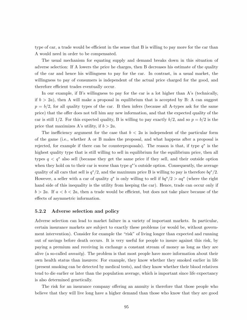
type of car, a trade would be efficient in the sense that B is willing to pay more for the car than

A would need in order to be compensated.

The usual mechanism for equating supply and demand breaks down in this situation of

adverse selection: If A lowers the price he charges, then B decreases his estimate of the quality

of the car and hence his willingness to pay for the car. In contrast, in a usual market, the

willingness to pay of consumers is independent of the actual price charged for the good, and

therefore efficient trades eventually occur.

In our example, if B’s willingness to pay for the car is a lot higher than A’s (technically,

if b > 2a), then A will make a proposal in equilibrium that is accepted by B: A can suggest

p = b/2, for all quality types of the car. B then infers (because all A-types ask for the same

price) that the offer does not tell him any new information, and that the expected quality of the

car is still 1/2. For this expected quality, B is willing to pay exactly b/2, and so p = b/2 is the

price that maximizes A’s utility, if b > 2a.

The inefficiency argument for the case that b < 2a is independent of the particular form

of the game (i.e., whether A or B makes the proposal, and what happens after a proposal is

rejected, for example if there can be counterproposals). The reason is that, if type q∗ is the

highest quality type that is still willing to sell in equilibrium for the equilibrium price, then all

types q < q∗ also sell (because they get the same price if they sell, and their outside option

when they hold on to their car is worse than type q∗’s outside option. Consequently, the average

quality of all cars that sell is q∗/2, and the maximum price B is willing to pay is therefore bq∗/2.

However, a seller with a car of quality q∗ is only willing to sell if bq∗/2 > aq∗ (where the right

hand side of this inequality is the utility from keeping the car). Hence, trade can occur only if

b > 2a. If a < b < 2a, then a trade would be efficient, but does not take place because of the

effects of asymmetric information.

5.2.2 Adverse selection and policy

Adverse selection can lead to market failure in a variety of important markets. In particular,

certain insurance markets are subject to exactly these problems (or would be, without govern-

ment intervention). Consider for example the “risk” of living longer than expected and running

out of savings before death occurs. It is very useful for people to insure against this risk, by

paying a premium and receiving in exchange a constant stream of money as long as they are

alive (a so-called annuity). The problem is that most people have more information about their

own health status than insurers: For example, they know whether they smoked earlier in life

(present smoking can be detected by medical tests), and they know whether their blood relatives

tend to die earlier or later than the population average, which is important since life expectancy

is also determined genetically.

The risk for an insurance company offering an annuity is therefore that those people who

believe that they will live long have a higher demand than those who know that they are good

95

risks (i.e., smokers whose fathers and grandfathers all died in their fifties). This forces insurance

companies to calculate with a lower mortality than the population average, which again makes

annuities even less attractive for good risks. They exit, and again insurers are forced to lower

the annuity that $1 buys, and so on. This is one of the reasons why most countries have a state

managed pension plan in which all people are forced to pay in. Similar problems also exist in

health insurance, with similar policy implications.

5.3 Signaling through education

Consider the following model of signaling through education. The population consists of two

different types. A proportion 1 − p is of type D (dumb), the remainder p is of type S (smart).

Once employed in firms, S types produce 20 units, while D types produce 10 units.

Unfortunately, firms cannot distinguish between D and S types, but they can observe x,

the level of education of a job applicant. Education in this model has no effect whatsoever on

productivity.2 The cost of education depends on the type: For smart types, it is σx. Without

loss of generality, we can set σ = 1. The cost for a dumb type is δx, where δ > 1. This just

means that reaching the same level of education is more expensive for a dumb individual, for

example because it takes longer to complete a degree or just because learning is more painful.

In this model, there are two different types of equilibria:

1. A separating equilibrium: The smart types choose a high level of education x, the dumb

ones choose x = 0. Employers believe that someone with education of (at least) x is smart,

and that everyone with less education is dumb.

2. A pooling equilibrium: No type (neither smart nor dumb people) obtains any education,

and everyone receives wage p · 20 + (1− p) · 10 = 10(1 + p).

We now analyze under which conditions these two types of equilibria exist. Consider first the

separating equilibrium: How high does x have to be in order that D-types do not imitate the

education level x of S-types? If a D-type takes his supposed equilibrium action and chooses

x = 0, employers will believe that he is a D-type and therefore he will receive a wage of 10.

Alternatively, our D-type could imitate the education level x that S-types obtain. This costs

δx, but the advantage is that firms will believe that our D-type is in fact an S-type and will be

willing to pay a wage of 20. The payoff from imitating the behavior of S-types for our D-type is

therefore 20− δx.

2I hope that you don’t consider this a feature that this class has, too! The point is not whether this assumption

is realistic. If education is productivity enhancing, then individuals have a legitimate reason to be educated. In

this model, we have removed all other reasons to get education apart from the signaling motivation to show most

clearly that signaling provides an incentive to receive education even if there is no other reason.

96

In an equilibrium, it must not be worthwhile for D-types to imitate S-types; otherwise, all

D-types would in fact imitate and then the belief of employers that someone who has obtained

education x is not justified. This implies that in a separating equilibrium, we must have x ≥ 10/δ.

The lowest education level that can support a separating equilibrium is therefore x = 10/δ.

The other question in a separating equilibrium is whether S-types do in fact find it optimal

to choose x = x? To check this, note that an S-type gets 20 − 10/δ. Since δ > 1, this is more

than 10, which is an S-type’s payoff if he imitates a D-type and does not get any education.

From a social point of view, education is wasteful in this model. Hence, if we weigh all

individuals’ utility the same, the state should prohibit education (this, of course depends on the

assumption that education is not productive at all). As for the different types, note first that

D-types always prefer the pooling equilibrium, because they just get a higher wage in the pooling

than in the separating equilibrium. For S-types, the situation is a bit more complicated: S-types

prefer the pooling equilibrium if 10(1 + p) > 20 − 10/δ, otherwise, they prefer the separating

equilibrium.

5.4 Moral Hazard

5.4.1 A principal-agent model of moral hazard

Economists talk about moral hazard in situations in which, after the contract is signed, the

behavior of one party is affected by the terms of the contract, and the change in behavior affects

the other party’s utility. The term “moral hazard” comes from the insurance sector and refers

to changes in loss prevention activities. Once an individual has bought insurance, he may not

be quite as careful any more in order to prevent the loss as he would be without insurance.

Insurance companies consider this behavior as “immoral”, hence the term.

One of the most important applications of moral hazard models is to incentives for workers

in firms. The owner of the firm, whom we call the “Principal” hires an agent to work for him;

think of a manager who actually directs the day-to-day operations of the firm. For simplicity, let

us assume that there are two possible output yh and yl, with yh > yl; we denote the probability

of a high output with p. The output level is observable and verifiable and so the salary can

depend on the level of output; let sh denote the worker’s salary when the output is yh, and sl

when the output is yl.

The agent can choose between two possible effort levels, eh and el, with eh > el. High

effort increases the probability of success, but is also more costly to the worker. Specifically, the

worker’s utility is

u = ph√sh + pl

√sl − ce, (5.1)

where ce is the cost of effort (either cl when effort is low, or ch when effort is high). The first

two terms are the worker’s expected utility from wage payments. We assume that the worker is

risk averse, and has a utility function equal to the square root function.

97

-

6

y (income)

u

0 shsl

.

.

.

.

.

.

.

.

.

.

.

.

.

.

.

.

.. . . . . . . �������������

u(sl)

u(sh)

.

.

.

.

.

.

.

.

.

.

.

.

.

.

.

.

.

.

.

.

.

.

.

.

.

.

.

.

.

.

.

.

.. . . . . . . . . . . . . . . . . . . . . . . . . . . . . .

Figure 5.1: Expected utility

Why do we assume this particular utility function for the worker, and what are the impli-

cations? The expected utility of the worker is a weighted average between√sl and

√sh, where

the weights are the respective probabilities for the events. Graphically, the expected utility

corresponds to a point on the line connecting the two points (sl,√sl) and (sh,

√sh), namely

(plsl + phsh, pl√sl + ph

√sh). The first coordinate of this point is the expected income, and the

second coordinate is expected utility. With the square root function (and other functions called

concave; those having decreasing first derivatives), the connecting line between two points that

are on the function is always below the function. That means that expected utility is below the

value of the utility function, evaluated at expected income: The worker would strictly prefer

to receive a certain amount of income that is equal to the expected income, to a “lottery over

income” (in which he sometimes gets more money and sometimes less, but which has the same

expected value). We call such a preference for certainty “risk aversion”, and the square root

function for expected utility is one function that has this property.

The principal, on the other hand, has a linear utility function, hence does not mind whether

he has a lottery or a certain amount of income (with the same expected value). It is generally

accepted that risk aversion is decreasing in income, i.e., rich people are (for a given risk) less

risk averse than poor people. Thus, the assumption that the principal is less risk-averse than

the agent is quite plausible (even though the assumption that he is completely risk-neutral is, of

course, less so; but that is not important). From the point of view of efficient risk-sharing, the

principal should take all the risk away from the agent. We can also say that he should “insure”

the agent against income risk.

98

Returning to the moral hazard problem, the relation between effort and success is given by

the following Table 5.1.

y = yh y = yl

e = eh 0.7 0.3

e = el 0.4 0.6

Table 5.1: Relation between effort and output

By exerting high effort, the agent is able to increase the success probability from 0.4 to 0.7.

Note that high effort increases success probability, but failure remains a possibility. Similarly, a

shirking worker may simply be lucky.

We now analyze how the optimal contract looks like. There are several cases to look at.

Case 1: Effort is observable and verifiable. In this case, the contract can specify the

effort level that the agent is required to choose. If, say, the contract specifies that the agent

has to exert high effort, but chooses only low effort, then the principal can take him to court

and receive a large penalty payment. hence, without loss of generality, we can assume that, if

the agent signs a contract that requires him to exert him effort, then he will exert high effort in

equilibrium.3 In addition, the contract may also specify that the wage depends on the output

level that has been realized.

Suppose first that the contract specifies that the agent has to exert high effort. The optimal

contract for the principal chooses the wage level sh and sl for high and low output, so as to

maximize

max 0.7(yh − sh) + 0.3(yl − sl) (5.2)

subject to the constraint that the worker is willing to sign the contract:

0.7√sh + 0.3

√sl − ch ≥ u. (5.3)

Here, u is the outside option of the worker, that is, the utility that the worker can get if he

works for another firm. Differentiating with respect to sh and sl yields the following first order

conditions:

−0.7 + 0.7λ

2√sh

= 0 (5.4)

−0.3 + 0.3λ

2√sl

= 0 (5.5)

3Of course it is not guaranteed that the optimal contract will indeed require high effort. Since the agent has

a higher cost of effort when exerting high effort, the wage payment necessary to induce the agent to sign a high

effort contract is likely to be larger than the wage payment under a low effort contract.

99

Solving both equations for λ yields λ = 2√sh = 2

√sl which implies sh = sl = λ2/4. We now

take this and substitute into the constraint (5.3) to get λ/2 = u+ ch ⇒ sh = sl = (u+ ch)2.

Let us now consider the optimal salaries under low and high output if the contract specifies

low effort. The principal’s problem is

max 0.4(yh − sh) + 0.6(yl − sl), (5.6)

subject to the participation constraint

0.4√sh + 0.6

√sl − cl ≥ u. (5.7)

The first order conditions are

−0.4 + 0.4λ

2√sh

= 0 (5.8)

−0.6 + 0.6λ

2√sl

= 0, (5.9)

From which we again find that sh = sl = λ2/4. When we substitute this into the participation

constraint, we get λ/2 = u+ cl ⇒ sh = sl = (u+ cl)2

Note that both contracts have “full insurance”, that is, the agent receives the same wage in

both output states; the principal assumes all the risk that is associated with the possibility of

low or high output. The intuition for this result is that the risk neutral principal (who maximizes

expected profit) assumes all the risk from the risk averse agent.

Which contract should the principal choose in Case 1, the one specifying high effort or the

one specifying low effort? The principal chooses the contract that gives a higher expected payoff.

The principal’s expected payoff from the high effort contract is

0.7yh + 0.3yl − (u+ ch)2. (5.10)

The principal’s expected payoff from the low effort contract is

0.4yh + 0.6yl − (u+ cl)2. (5.11)

If 0.3(yh − yl) > (u + ch)2 − (u + cl)2, then the high effort contract is better for the principal,

otherwise, it is the low effort contract.

Case 2: Effort is unobservable/unverifiable. In this case, the contract cannot specify the

effort level of the agent. Observe first that a full insurance contract will lead to low effort by the

worker, because, if the worker does not receive any different wage depending on output, then

he has no incentive to choose the high effort that is more costly. Note also that the optimal low

effort contract from Case 1 above remains feasible.

100

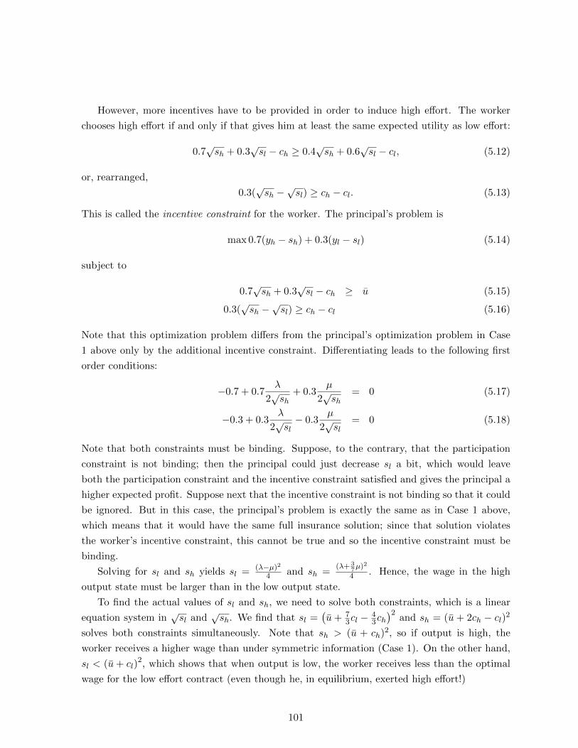
However, more incentives have to be provided in order to induce high effort. The worker

chooses high effort if and only if that gives him at least the same expected utility as low effort:

0.7√sh + 0.3

√sl − ch ≥ 0.4

√sh + 0.6

√sl − cl, (5.12)

or, rearranged,

0.3(√sh −

√sl) ≥ ch − cl. (5.13)

This is called the incentive constraint for the worker. The principal’s problem is

max 0.7(yh − sh) + 0.3(yl − sl) (5.14)

subject to

0.7√sh + 0.3

√sl − ch ≥ u (5.15)

0.3(√sh −

√sl) ≥ ch − cl (5.16)

Note that this optimization problem differs from the principal’s optimization problem in Case

1 above only by the additional incentive constraint. Differentiating leads to the following first

order conditions:

−0.7 + 0.7λ

2√sh

+ 0.3µ

2√sh

= 0 (5.17)

−0.3 + 0.3λ

2√sl− 0.3

µ

2√sl

= 0 (5.18)

Note that both constraints must be binding. Suppose, to the contrary, that the participation

constraint is not binding; then the principal could just decrease sl a bit, which would leave

both the participation constraint and the incentive constraint satisfied and gives the principal a

higher expected profit. Suppose next that the incentive constraint is not binding so that it could

be ignored. But in this case, the principal’s problem is exactly the same as in Case 1 above,

which means that it would have the same full insurance solution; since that solution violates

the worker’s incentive constraint, this cannot be true and so the incentive constraint must be

binding.

Solving for sl and sh yields sl = (λ−µ)24 and sh =

(λ+ 37µ)2

4 . Hence, the wage in the high

output state must be larger than in the low output state.

To find the actual values of sl and sh, we need to solve both constraints, which is a linear

equation system in√sl and

√sh. We find that sl =

(u+ 7

3cl −43ch)2

and sh = (u + 2ch − cl)2

solves both constraints simultaneously. Note that sh > (u + ch)2, so if output is high, the

worker receives a higher wage than under symmetric information (Case 1). On the other hand,

sl < (u+ cl)2, which shows that when output is low, the worker receives less than the optimal

wage for the low effort contract (even though he, in equilibrium, exerted high effort!)

101

The principal’s expected profit, when choosing a high effort inducing contract, is

0.7yh + 0.3yl − expected wage (5.19)

Using the results from above, the expected wage is

0.7 (u+ 2ch − cl)2 + 0.3

(u+

7

3cl −

4

3ch

)2

>[0.7 (u+ 2ch − cl) + 0.3

(u+

7

3cl −

4

3ch

)]2= (u+ ch)2

(5.20)

Because (u+ ch)2 is the wage that the principal would have to pay if effort were observable and

verifiable, the principal is worse off than under observable effort. There are now two possibilities.

The first one is that it is still optimal for the principal to use a contract that is meant to induce

high effort, even though this is now more expensive (in expectation) than under symmetric

information. Second, it is possible that under asymmetric information, the expected profit

under the high effort contract goes down by so much that now the low effort contract becomes

better for the principal.

In either case, there is a welfare loss due to asymmetric information. Since the agent reaches

exactly the same (expected) utility as in Case 1, the difference in the principal’s profit measures

the welfare loss.

5.4.2 Moral hazard and policy

Moral hazard is an important problem in many economic settings, wherever individuals respond

to “insurance” by changing their behavior in a way that is unfavorable for the principal. The

following are just some examples:

• Contracts for managers (problems: shirking; “empire building”

• certain insurance contracts (problem: reduced self-protection)

• procurement (e.g., buy fighter jets; if state reimburses costs, firm does not have an incentive

to reduce costs)

• Social assistance programs (e.g., unemployment insurance; problem: individuals may re-

duce effort when looking for a new job)

• taxation (higher marginal tax rate reduces incentives to work longer or increase produc-

tivity by education)

Other than in the first two applications of asymmetric information (i.e., adverse selection and

signaling), there is no obvious policy recommendation in the case of moral hazard. The state

does not have any particular advantage over private parties, when moral hazard is an issue: The

state as principal needs to give incentives to its agents, too, pretty much in the same way as

private parties.

102

Part III

Social choice and political economy

103

Chapter 6

The Social Choice Approach to

Political Decision Making

6.1 Introduction

In the last chapter, we have analyzed the welfare properties of a market equilibrium, in particular

(in the First Theorem of Welfare Economics) a specific scenario in which the market outcome is

socially optimal, and then a sequence of problems in which the market outcome is not optimal,

in the sense that a benevolent “social planner” can do better for all parties involved. These

market failures, and the state’s ability to correct some of these, constitute the fundamental

philosophical basis for the existence of a state.

Of course, in reality, the decisions on how exactly the government should act are contentious

(individuals in society rarely agree unanimously on which policy the government should im-

plement, because policies have different effects on different people) and not made by a social

planner. Rather, they are the outcome of political processes in which self-interested individuals

(voters, politicians, judges, bureaucrats) interact with each other.

In the present chapter, we take a particular approach to policy-making that does pre-suppose

a particular institutional setting and analyzes the actions of agents with this institutional setting

(we will do that in later chapters). Rather, we consider a question of institutional design: If we

could set up rules and procedures from scratch, are any “reasonable” aggregation procedures

that take the preferences of all individuals as input and produce a “reasonable” social ranking

of alternatives as output. (Of course, we will need to specify explicitly what we want to consider

as “reasonable” requirements for our rules).

The opportunity to engage in institutional design is usually rare because institutions are

usually set up in a way that they are hard to change. For example, the U.S. constitution

requires a two-thirds supermajority in both houses of Congress and the ratification by three-

fourths of the states for an amendment (a change or addition to the constitution) to pass. As

104

a consequence, fundamental changes to the constitution are very hard to pass. This shows that

it is really important to implement the “correct” rules for social decision making right from the

beginning.

In this chapter, we deal with a particular approach to institutional design that was pioneered

by Kenneth Arrow in the 1950s. Arrow defines some features that would be desirable for any

preference aggregation institution (i.e., a set of rules for how society comes up with social

decisions that are made jointly and that apply to all members). Arrow’s famous impossibility

theorem shows that, for general preferences among the voters, no aggregation procedure satisfies

these desirable features simultaneously. This shows that all conceivable voting rules, apart from

their respective advantages, necessarily also have disadvantages. There is no “perfect” rule that

satisfies all desirable features, but rather advantages and disadvantages for each.

A result that is closely related to Arrow’s Impossibility Theorem is the Gibbard-Satterthwaite

Theorem that shows that democratic social choice function that aggregates individual preferences

can be “strategy-proof”; that is, for essentially any mechanism of aggregation of preferences over

more than two possible choices, there are cases in which individual voters would be better off

if they “misrepresent” their true preferences. This is a significant concern in practice: Any

social decision mechanism requires that individual voters take some action, for example, rank

all candidates or vote for one or more candidates.

An example for such strategic behavior is the choice of voters in plurality rule elections who

prefer one of the minor candidates, i.e., a candidate who is generally thought of as not having

a chance to win, because his support base is smaller than the ones of the two main contenders

(think Ralph Nader in the 2000 U.S. Presidential election). Such a voter can either vote for his

preferred candidate and “waste his vote” (in the sense of having no chance for influencing the

identity of the election winner), or “vote strategically” for the candidate among the relevant

candidates whom he likes more (or considers the “lesser evil”). The Gibbard-Satterthwaite

Theorem indicates that strategic voting does not only arise under plurality rule, but under any

reasonable mechanism. A thorough analysis of voting systems therefore has to take into account

the incentive for voters to behave strategically.

6.2 Social preference aggregation

When individuals exchange goods or write other contracts in market context, a contract requires

that both parties (or all involved parties) agree in order for a deal to go forward. We could say

that there is a “unanimity principle” for private contracting. In contrast, social decision making

affects many people and is usually subject to non-unanimous decision rules. For example, the

state governor is elected by plurality rule in most U.S. states (i.e., the candidate who receives

the most votes wins), and always there are at least some voters who do not agree with the choice

of the majority. Whenever there is disagreement about the ranking of alternatives, there needs

105

to be a rule how the social ranking is determined in these cases.

Specifically, Arrow’s Theorem analyzes preference aggregation mechanisms that deal with a

society that has to rank a set of several, mutually exclusive alternatives. For example, in some

sports disciplines such as figure skating, a panel of judges has to determine the rank-order of the

different participants; that is, in the Olympics, they have to decide who wins the gold medal, the

silver medal and so on.1 In what follows, we would call the judges in this example the “voters”

and the contestants the “candidates”.

A ranking is simply a list of all the candidates that states who is the first place candidate,

the second place, the third one and so on. A preference aggregation mechanism is a set of rules

that determines how the opinions of the different judges map into a ranking of the candidates.

For example, each judge could award points to each of the contestants, and then the ranking is

determined by the contestants’ aggregate score from all judges – this is a particular example of

a preference aggregation mechanism.

6.2.1 Review of preference relations

We are concerned with determining a social ranking over a set of candidates. Preference rankings

over a set of alternatives also play a big role in household theory, and many of the concepts and

notations used there are useful for the problem at hand. For this reason, we start by reviewing

some properties of preference relations.

A central role is played by the preference relation �. In household theory, � stands for

“weakly better than” or “weakly preferred to”, such as in the statement “the bundle consisting

of 2 apples and 3 bananas is weakly better than the bundle consisting of 1 apple and 4 bananas”,

which we can write (2, 3) � (1, 4).2 (Of course, this is an individual’s personal preference, not

a general rule; you might equally plausibly find that (1, 4) � (2, 3)). The “weak” part in the

statements indicates that indifference is included. That is, (2, 3) � (1, 4) is also satisfied for

an individual who is indifferent between the bundle consisting of 2 apples and 3 bananas, and

the bundle consisting of 1 apple and 4 bananas. In this case, it is of course also true that

(1, 4) � (2, 3), and we can also denote indifference by (1, 4) ∼ (2, 3). In contrast, (2, 3) � (1, 4)

denotes a strict preference for the first bundle.

We now turn to a couple of properties that reasonable preference relations should satisfy.

Definition 3. A relation � on X is called

(i) Complete, if ∀x, y ∈ X, either x � y or y � x.

1Note that it is not the case that only the first three ranks as determined by the judges are significant. For

one, one or more presumptive medal winners may become ineligible for a medal, for example because of doping

which usually is not discovered until after the competition has ended. In this case, we need to know who is the

next in line for a medal. Furthermore, national sports federations often condition their aid on reaching a top-10

(or top-whatever) position in international championships or the Olympics.2Here, (q1, q2) denotes the bundle of goods composed of q1 apples and q2 bananas.

106

(ii) Transitive, if for all x, y, z ∈ X, if x � y and y � z then x � z.

(iii) Rational, if it is complete and transitive.

Completeness means that all elements of the set X (e.g., all bundles of goods in a given

budget set, or all candidates in our political framework) can be compared by the relation. For

two elements, say x and y, the individual feels either that x is at least as good as y, or y is at

least as good as x, or possibly both. In the latter case, the individual is indifferent between x

and y. However, the individual never says “gosh, I don’t know, I cannot compare x and y”.

In a political election context, completeness may not necessarily be satisfied in practice:

If there are, say, ten candidates in a presidential election, then chances are that most voters

probably have not heard from at least 7 of these candidates and may be unable to say which of

them they prefer over another one. However, this is in principle just a problem of information

and (rational) ignorance of the part of voters: If minor candidates have no chance of winning the

election, then it makes no sense for a voter to invest time in learning how he should rank these

candidates. However, if it really mattered, then voters could certainly learn their preferences.

Transitivity means that there are no “chains” of objects such that the individual’s preference

reverses along a chain. If an individual likes x better than y, and y better than z, then the

individual should also like x better than z. Transitivity is a property usually identified with

rationality, and there is a strong evolutionary argument in favor of transitivity: An individual

who does not satisfy transitivity could be offered a sequence of trades that are all acceptable

for him because he receives a “better” bundle, but ultimately, he ends up in a strictly worse

situation than before.3

If individual preferences were not complete or transitive, we could not expect that a social

preference aggregation mechanism suddenly acquires these properties. Therefore, we will assume

that individual voters’ preferences that we use as input for the aggregation mechanism satisfy

both completeness and transitivity.

Finally, as already indicated above, we can derive two other relations from the preference

relation �.

Definition 4. 1. Strict preference �: x � y, if and only if x � y but not y � x (x is strictly

preferred to y).

2. Indifference ∼: x ∼ y if and only if x � y and y � x (x is as good as y, or x and y are

indifferent).

In most cases, we will assume that there is a finite set of candidates, and that individual voters

have strict preferences between different candidates (i.e., they are never indifferent between two

3The fairy tale “Hans in Luck” in which the protagonist starts out with a lump of gold and sequentially trades

his possessions to eventually end up with a grindstone is an example of such an individual with non-transitive

preferences.

107

V1 V2 V3

most preferred A B C

middle B C A

least preferred C A B

Table 6.1: Voter preferences that induce the Condorcet paradox

different candidates). This sometimes simplifies arguments and proofs, and is often reasonable

because it is very unlikely that two different options from a finite set of candidates give a voter

exactly the same utility. However, the assumption is never required for the logical validity of

results.

6.2.2 Preference aggregation

We are now equipped to start our analysis of preference aggregation. Suppose we have a society

of n voters, each with rational preferences over three or more distinct and mutually exclusive

decisions (for example, candidates for the presidency or different sales tax rates imposed on

citizens, with corresponding public spending).

We call the list of all voters’ preferences, {�1, . . . ,�N} ≡ {�i}i=1...N = p a preference profile.

For example, consider Table 6.1 where there are three voters (V1, V2 and V3) who have different

preferences over the three candidates (A, B and C). This table is an example for a preference

profile.

A preference aggregation mechanism is a function that maps the set of all possible preference

profiles into the set of possible social rankings for all pairs of candidates. Let us first talk

about the domain of this function, the set of all possible preference profiles. Consider the

setting of Table 6.1 with 3 voters and 3 candidates (this is really one of the simplest interesting

settings), and suppose furthermore that we restrict the voter preferences to be considered to

strict preferences (i.e., no voter is indifferent between any two candidates). For each voter,

there are 6 different possible preference rankings: ABC, ACB, BAC, BCA, CAB and CBA.

Since there are three voters, the number of different preference profiles is therefore 63 = 216.

In general, for k candidates, the number of different strict preference rankings is k!, and when

there are n voters, there are (k!)n different preference profiles. Note that this number grows

large very quickly when k and/or n grows.

How about if we admit ties in the preference rankings of voters? As above, there are 6 strict

preference rankings. Furthermore, consider rankings where two candidates are tied: There are(32

)= 3 ways to select a group of two tied candidates (namely A and B; A and C; B and C),

and the tied candidates can be tied for the first place or for the second place in the ranking.

Thus, there are 6 different social rankings in which exactly 2 candidates are tied. Finally, there

108

is one ranking in which all candidates are tied. Thus, if we admit ties in individual preference

profiles, then even in the most basic example of 3 voters with 3 candidates, our domain consists

of 133 = 2197 different preference profiles.

Each of these is now mapped, by the mechanism into a social preference over the set of all

pairs of candidates. In our example, this means that the mechanism tells us whether A � B

or B � A or both; whether A � C or C � A or both; and whether B � C or C � B or

both. Clearly, if there are more candidates, then the output of the social preference aggregation

mechanism consists of a comparison of all pairs of candidates.

For example, consider the “plurality mechanism” which is defined as follows: For each can-

didate, we count the number of voters who rank this candidate highest. Then, we rank the candi-

dates according to this count, i.e., we say that x � y if and only if #{voters who rank x highest} ≥#voters who rank y highest. Here, “#K” means “the number of elements of set K”. With the

example electorate of Table 6.1, each candidate has one supporter, so A ∼ B, A ∼ C and B ∼ C.

Combining these pairwise comparisons, we could express this three-way tie in the social ranking

as A ∼ B ∼ C. Note that this example shows that, even if all voters have strict preferences, it

may be the case that the social ranking has a tie between some (or all) of the candidates.

Also, related to the description of the plurality mechanism above, experience with student

answers induce me to state that, in this and all following descriptions of mechanisms, x and y

are placeholders for the names of two generic candidates. That is, the rule described applies

for all pairs of candidates, and not just for the two called x and y (there may not be any with

those names, anyway). So, if the set of the candidates is {A,B,C}, then A � B if and only if

#(voters who rank A highest) ≥ #(voters who rank B highest) and so on.

The approach to defining the ranking by a relation on all subsets of two candidates may

seem unnecessarily complicated. Why not just say that a preference aggregation mechanism

produces a “linear ranking” in the sense that the mechanism produces a list that tells us which

candidate is first, second, third and so on. Such a linear ranking contains all information about

pairwise comparisons, but is usually much tidier/shorter. For example, if there are 5 different

candidates, then there are(52

)= 10 different pairs of candidates, while a linear social ranking

would just list the 5 candidates in some order.

So, why not stating the output of the preference aggregation mechanism in this simpler way?

The problem is that there are many practically important preference aggregation mechanisms

that sometimes (i.e., for some preference profiles) produce intransitive rankings.

The most important example of such a mechanism is the simple majority preference: For a

given voter preference profile p and for any two candidates x and y, we count the number of

voters who strictly prefer x over y, and the number of voters who strictly prefer y over x. If

there are strictly more voters of the first type (i.e., x-supporters), then we say that x is socially

preferred to y, and vice versa. If the number of x- and y-supporters is the same, then we say

109

that x and y are socially indifferent. Formally,

x �S y ⇐⇒ #{i : x �i y} > #{i : y �i x}

x ∼S y ⇐⇒ #{i : x �i y} = #{i : y �i x}(6.1)

If we apply this mechanism to the preferences in Table 6.1, we find that A � B, B � C and

C � A: Simple majority preference may be intransitive! This surprising result, known as the

Condorcet paradox is named after the 18th century French mathematician (and voting theorist)

Nicolas Marquis de Condorcet.

The Condorcet paradox indicates a fundamental problem with democratic decisions made

by simple majority rule. One possible way to select a winning candidate using a simple majority

rule would be the following. We start with an “election” between candidates A and B; whoever

wins more votes then goes up against C, and so on until we have reached the last candidate.

The winner of that final election is the overall winner. If we have a social preference profile such

that simple majority preference is transitive, then this algorithm is guaranteed to converge to

the candidate placed highest in the social ranking.

For example, suppose that the voter preference profile is such that D �M A �M BsuccMC

is the (transitive) majority ranking. Then A would win the first election against B and the

second one against C, but lose the final election against D. While the final winner (D) did not

compete head-to-head with B and C, he would also win those elections provided that majority

preferences are transitive. So, after the final election, it would not be possible to suggest a

different candidate who would gather a majority when paired against the final winner.

In contrast, what happens if the preference profile is such as in Table 6.1? In this case, A

wins the first election against B, and loses the final election against C. But the “final winner”

(C) never competed against B and would actually lose that election against B by majority. So,

after the algorithm results in C winning, a majority (namely the voters who prefer B over C)

could be mobilized to have “one more vote”. And, of course, if that vote happened, it would

not be the end of the story either because then there would be a majority of voters who prefer

A over B. And so on, without end.

Of course, we could just impose that voting ends after all candidates have competed in at

least one election. This way, there is always a final winner. However, this approach just shifts

the problem. If majority preferences are intransitive, then the sequence of voting matters for the

outcome. For example, if the first election is not A versus B but rather A versus C, then C wins

the first election, and B wins the final election. If, instead, the first election is B versus C, then

B beats C, but loses in the final election against A. Thus, depending on the sequence in which

the electorate votes on the candidates, a different winner emerges. This points to an important

role of whoever gets to decide the agenda (the sequence of voting) when majority preferences are

intransitive. In contrast, if majority preferences are transitive, then the sequence in which the

electorate votes on the candidates does not matter for the final outcome (you should confirm

110

this for the example above with transitive majority preferences). We will come back to this

example in the section on the Gibbard-Satterthwaite theorem.

6.3 Desirable properties for preference aggregation mechanisms:

Arrow’s axioms

Up to now, we have just defined a preference aggregation mechanism as a mapping from the

set of all possible voter preference profiles to the set of possible social rankings for all pairs

of candidates. So far, we have imposed no restrictions on that mapping. Many potential

aggregation mechanisms are very weird. For example, consider the “indifference mechanism”

that essentially refuses to rank candidates: “For any pair of candidates x and y and for all voter

preference profiles p, x ∼ y.”

This is a preference aggregation mechanism because, for any voter preference profile, it

tells us the social ranking between any pair of candidates (which is always the same, namely

indifference, for this mechanism). Nevertheless, the mechanism strikes us as a stupid way to

“aggregate” social preferences. For example, even for those voter preference profiles in which all

voters agree that A � B, the mechanism tells us that A and B are socially indifferent.

In this section, we want to define more precisely what we mean by “a stupid way to aggregate

preferences,” so that we can exclude these mechanisms from further consideration. Or, positively

speaking, what are the minimum properties that we should require from a preference aggregation

mechanism? We now present a list of five requirements that are known as Arrow’s axioms.

As before, we use x, y and z to denote generic candidates in the following definitions,

i.e., these definitions should hold for any pair (or triple) of candidates. A generic individual

voter’s preference ranking is denoted �i. A generic preference profile, {�1,�2, . . . ,�i, . . . ,�n}is denoted p. Finally, the output of the preference aggregation mechanism, the social preference,

is denoted�S . (Note that, through the aggregation mechanism, the social preferences�S depend

on the voter preference profile p, so we could denote this dependence explicitly as �S (p), but

usually, we will not do this.)

Completeness (C): For any p and any pair of candidates x and y, either x � y or y � x (or

both).

This axiom just says that the aggregation procedure returns a social preference relation

�S between any pair of candidates. In principle, one could say that this axiom is already

embodied in the definition of a mechanism, since a mechanism has the entire set of pref-

erence profiles as its domain (i.e., it maps every conceivable voter preference profile p into

a social preference ranking).

However, it is useful to spell this property out explicitly: If we are given a description of

a particular procedure to aggregate preferences, we need to check whether this procedure

111

really provides a social ranking for all possible preference profiles.

As an example, suppose that a friend suggests the following “unanimity” procedure: “For

any pair of candidates x and y, x �S y if and only if x �i y for every voter i.” This

procedure violates Completeness (or, we could say, it is not a mechanism). Sure, if every

voter prefers x to y, then this procedure ranks x as socially preferred to y, and vice versa

if everyone prefers y to x. However, if neither support for x nor for y is unanimous (and

there are very many preference profiles where this is the case), then the mechanism does

not return a social preference. So, for your friend’s procedure suggestion to be an actual

preference aggregation mechanism that satisfies Completeness, he needs to also spell out

explicitly what the social ranking of two candidates should be if voters disagree on the

ranking of these two candidates. We will return to such an amended unanimity mechanism

below.

Transitivity (T): For any p, if x �S y and y �S z, then x �S z. In words, the social aggre-

gation mechanism produces a transitive ranking for all possible voter preference profiles

p.

Remember that we assume that the individual voters’ preferences are both complete and

transitive. What the axioms C and T require is that these properties of individual ratio-

nality do not get lost in aggregation: Like all individual rankings, the social preference

ranking should also be complete and transitive.

Our earlier example with the preferences of Table 6.1 shows that the simple majority rule

preference aggregation mechanism violates the transitivity axiom. Note that, to draw that

conclusion, all we need is an example where for a particular preference profile, the social

preference ranking generated by the simple majority mechanism is not transitive.

It is certainly true that simple majority preference can lead to transitive social preferences

(for some preference profiles). A simple example for such a case is when all individual voters

have the same preference ranking; in this case, the social preference ranking generated

by simple majority rule is exactly the same as the one that all voters have, and that

ranking is transitive. However, for the transitivity axiom to be violated, all we need is

one preference profile for voters where simple majority rule generates intransitive social

preferences. This is because the logical opposite of “for all preference profiles p, the social

ranking is transitive” is “not for all preference profiles p, the social ranking is transitive”,

and the latter statement is equivalent to “for some preference profiles, the social ranking

is not transitive”.

Pareto (P):

x �i y for all i and x �i y for some i implies x �S y

Remember the example of the indifference mechanism from the beginning of this section.

112

This mechanism satisfies C and T (check this!), but it struck us as weird because the social

ranking was always the same and was completely independent of the voters’ preferences.

Even if every voter preferred x to y, the indifference mechanism still raked those candidates

as x ∼S y.

This is clearly an undesirable property, and axiom P is meant to exclude such mechanisms.

P requires that, if all voters agree that x is better than y, in the sense that nobody thinks

that y is strictly better than x and at least some people think that x is strictly better than

y (i.e., if if x is weakly Pareto better than y), then the social preference ranking should

respect this judgment and rank x above y.

Note that this is a very weak requirement. If voters disagree about two candidates (i.e.,

there is at least one voter who prefers x to y, and some other voter who prefers y to x;

this is likely the standard case in large societies), then the requirement P does not im-

pose any restrictions on the preference aggregation mechanism. For non-unanimous voter

preferences, all mechanisms are compatible with P. The only cases in which P represents

a true test in the sense that it can fail is if all voters agree. In this case, the mechanism

should reflect that preference which is shared by everybody.4

Independence of Irrelevant Alternatives (IIA): This axiom applies to the social ranking

of a pair of candidates, x and y, in two situations in which voter preferences in general

differ, but are “comparable” when just looking at each voter’s preferences over x versus y.

Specifically, let p = {�1, . . . ,�n} and p′ = {�′1, . . . ,�′n} be two different voter preference

profiles, but suppose that, for all individuals, the preference relation between the pair of

candidates x and y is the same in both profiles i.e.

x �i y ⇐⇒ x �′i y (6.2)

That is, each voter’s preferences in p and p′ may differ in the sense that (for example)

voter i prefers z over both x and y in preference profile p, but has x �′i z �′i y in preference

profile p′.

Whenever this is true, we want that the social preference aggregation returns the same

social preference over x vs y for both preference profile p and p′, i.e.

x �S y ⇐⇒ x �′S y. (6.3)

4Experience with students in earlier years induces me to state that, obviously, P does not require that “all

voters agree in their ranking of candidates”. This would be non-sense, both practically (very rarely is it the case

that everybody agrees, so such a requirement would essentially rule out all interesting cases) and logically (we

make requirements concerning what the aggregation mechanism should or should not do; but we do not make

assumptions how voter preferences look like; in fact, we require the mechanism to work for any voter preference

profile.

113

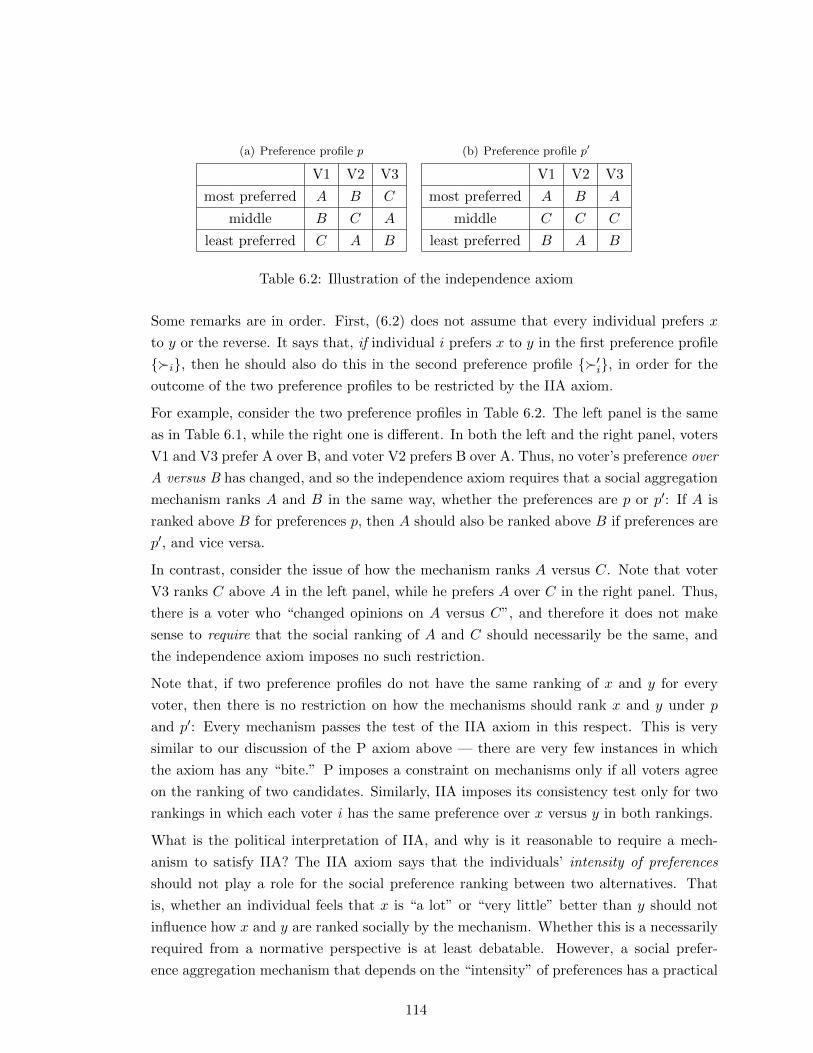
(a) Preference profile p

V1 V2 V3

most preferred A B C

middle B C A

least preferred C A B

(b) Preference profile p′

V1 V2 V3

most preferred A B A

middle C C C

least preferred B A B

Table 6.2: Illustration of the independence axiom

Some remarks are in order. First, (6.2) does not assume that every individual prefers x

to y or the reverse. It says that, if individual i prefers x to y in the first preference profile

{�i}, then he should also do this in the second preference profile {�′i}, in order for the

outcome of the two preference profiles to be restricted by the IIA axiom.

For example, consider the two preference profiles in Table 6.2. The left panel is the same

as in Table 6.1, while the right one is different. In both the left and the right panel, voters

V1 and V3 prefer A over B, and voter V2 prefers B over A. Thus, no voter’s preference over

A versus B has changed, and so the independence axiom requires that a social aggregation

mechanism ranks A and B in the same way, whether the preferences are p or p′: If A is

ranked above B for preferences p, then A should also be ranked above B if preferences are

p′, and vice versa.

In contrast, consider the issue of how the mechanism ranks A versus C. Note that voter

V3 ranks C above A in the left panel, while he prefers A over C in the right panel. Thus,

there is a voter who “changed opinions on A versus C”, and therefore it does not make

sense to require that the social ranking of A and C should necessarily be the same, and

the independence axiom imposes no such restriction.

Note that, if two preference profiles do not have the same ranking of x and y for every

voter, then there is no restriction on how the mechanisms should rank x and y under p

and p′: Every mechanism passes the test of the IIA axiom in this respect. This is very

similar to our discussion of the P axiom above — there are very few instances in which

the axiom has any “bite.” P imposes a constraint on mechanisms only if all voters agree

on the ranking of two candidates. Similarly, IIA imposes its consistency test only for two

rankings in which each voter i has the same preference over x versus y in both rankings.

What is the political interpretation of IIA, and why is it reasonable to require a mech-

anism to satisfy IIA? The IIA axiom says that the individuals’ intensity of preferences

should not play a role for the social preference ranking between two alternatives. That

is, whether an individual feels that x is “a lot” or “very little” better than y should not

influence how x and y are ranked socially by the mechanism. Whether this is a necessarily

required from a normative perspective is at least debatable. However, a social prefer-

ence aggregation mechanism that depends on the “intensity” of preferences has a practical

114

weakness: Nobody but the individuals themselves knows how “intensive” they feel about

the alternatives, and it appears likely that individuals would misrepresent the intensity of

their preferences.5

The IIA axiom is also related to the fact that individual preferences in economic theory

are defined only up to an ordinal transformation. That is, economists cannot interpret the

difference between the two statements “x is a bit better than y for individual i” and “x is

a lot better than y for individual i” in any precise way.

No Dictator (ND). The previous axioms can easily be satisfied by singling out one individual

d as the “dictator” who is the only member of society whose preferences count, i.e. x �S ywhenever x �d y. However, this can hardly be called a “social” preference aggregation

mechanism, since there is only one individual who counts in all circumstances. A minimum

requirement for even the slightest “democratic” appeal of a social preference aggregation

mechanism is that there is no single individual whose preferences always determine what

the social preferences are, for all possible preference profiles.

Note that this is a very weak requirement satisfied by a lot of mechanisms in which one

individual voter is very powerful (without being a dictator for all circumstances). Consider,

for example, a mechanism such that the social preference order is equal to individual

1’s preference order, unless all other individuals have the same preference order that is

different from 1’s, in which case their preference order counts as the social preference

order. Very likely, there is some disagreement among the other voters, so this mechanism

gives individual 1 a lot of power and we would not consider it to be very “democratic”;

yet it satisfies the ND axiom.

A stronger alternative to the ND axiom would be some sort of symmetry requirement

between voters. For example, when p and p′ are two social preference profiles that are pure

permutations of each other (i.e., for each individual with a certain preference ordering in

p, there is an individual who has exactly the same preference ordering in p′), a symmetry

axiom would require that the social preference ordering generated by the mechanism is

exactly the same under p and p′. Clearly, every mechanism that satisfies such a symmetry

axiom automatically satisfies the ND axiom.6

While such a symmetry requirement would perhaps be more appealing if the objective

5When the stakes in the social decision are small, this may be less of a problem. Consider, for example, the

problem of choosing (or rescheduling) a midterm date for a class. Usually, when I ask a class to vote for which

date they prefer, a substantial fraction of the class abstains. It is unlikely that all abstainers are really completely

indifferent between the two proposed dates. More likely, they feel that their own very weak preferences for one of

the dates should not (in an ethical sense) influence the scheduling outcome.6To see this, suppose that we have a dictator mechanism: If the dictator’s preferences are exchanged with an-

other individual’s ranking, the social ranking changes (to the dictator’s new ranking). Consequently, a dictatorial

mechanism violates symmetry. Thus, a symmetric mechanism must be non-dictatorial.

115

was to construct the ideal mechanism, Arrow’s Theorem shows that it is not even pos-

sible to construct a mechanism that satisfied all five axioms simultaneously. This result

becomes the more powerful, the weaker the requirements are that the axioms impose. In

other words, whatever “more reasonable” (stronger) requirements we impose on the social

aggregation mechanism will also lead to an impossibility result.

6.3.1 Examples of social aggregation procedures

We now discuss some social preference aggregation mechanisms and see which axioms they

satisfy and which ones they fail. Consider first the

Unanimity rule. Consider first the following unanimity rule without status quo: If everyone

prefers x to y, then the unanimity rule mechanism ranks x as socially preferred to y. If everyone

prefers y to x, then the unanimity rule mechanism ranks y as socially preferred to x. If neither

support for x nor for y is unanimous, then the mechanism does not return a social preference.

Formally,

x �S y ⇐⇒ x �i y for all i (6.4)

Which properties are satisfied by unanimity rule?

• Completeness clearly fails, because there are profiles of individual preferences such that

neither support for A nor for B is unanimous, and in these cases the mechanism does

not return a social preference. Whenever unanimity rules are applied in practice, there

must be a specification for what happens if no candidate (or proposal) receives unanimous

consent by all voters. We will return to this point below.

• Transitivity is satisfied. To see this, note that if we know that x �S y, then x �i y for all

i. Similarly, if y �S z, then y �i z for all i. Since all individual have transitive preferences,

this implies that x �i z for all i, and hence x �S z.

• Pareto optimality, which is just the requirement that

x �S y ⇐ x �i y for all i (6.5)

clearly is implied by (6.4).

• Independence of irrelevant alternatives also holds. If all individuals prefer x over y in

preference profile p and rearranging leaves the ordering of x vs. y unaffected for each

individual, then also in preference profile p′, all individuals prefer x over y and so the

social preference remains x �S y.

• Last, No Dictator also holds. Sometimes, students argue that “all individuals are dictators”

under unanimity rule, but the dictator condition ND does not say that nobody should be

116

V1 V2 V3

most preferred C C B

middle A B C

least preferred B A A

Table 6.3: Example: Extended unanimity rule violates the transitivity axiom

able to block a decision, only that nobody should be able to enforce his will on other people

all of the time. Clearly, this is not the case under unanimity rule: No individual can impose

his preferences over x vs. y (for any pair of candidates) on the social ordering all of the

time, because even a single other individual who does not share the first individual’s view

means that society cannot rank x and y.

How could we extend the definition of unanimity rule to provide for completeness? One

possibility is to resort to an exogenous ranking of candidates whenever there is no unanimous

consent. In most practical applications of unanimity rule, there is a status quo that remains

in force as long as there is no unanimous consent to overturn it (e.g., U.N. security council;

admission to the European Union). Remember, though, that our problem here is slightly differ-

ent: A preference aggregation mechanism needs to rank all of the candidates (not just a single

candidate “change of the status quo” against the default candidate “status quo”).

We could do this as follows. Let x and y be two candidates who are ordered according to an

exogenous ranking (for example, the alphabetic order of their names), with x ranked before y.

Then, in the social ranking x � y unless y is Pareto better than x. Formally

y �S x if y �i x for all voters i and y �j x for at least some voter j

x �S y otherwise

This extended unanimity rule is clearly complete, because for any pair of candidates, either all

voters agree (in a Pareto-better sense), in which case the social ranking follows their preferences,

or voters disagree, in which case the social ranking follows the exogenous ranking. Clearly, the

extended unanimity rule still satisfies the Pareto axiom and the No Dictator axiom (because

again no individual can impose his preferences independent of the other voters). Independence

of Irrelevant alternatives is also satisfied: If the preference profile changes from p to p′, and all

voters in p′ have the same preferences over x versus y as they had in p, then the social ranking

of x and y in the extended unanimity mechanism does not change.

However, the extended unanimity mechanism fails Transitivity. To see this, consider the

following example of voters preferences given in Table 6.3.

Since voters disagree on A versus B, and A is ranked earlier in the alphabet, A �S B.

Similarly, voters disagree on B versus C, and B is ranked earlier in the alphabet, so B �S C.

117

(a) Preference profile

p

V 1 V 2 V 3

x y z

y z x

z w y

w x w

(b) Preference profile

p′

V 1 V 2 V 3

x y z

y x x

z z y

w w w

Table 6.4: IIA is violated for Borda rule

However, all voters agree that C is better than A, so C �S A, while transitivity would require

that A �S C (given the first two comparisons).

In summary, fixing the unanimity mechanism’s problem with completeness is possible, but

comes at the cost of generating a new problem with transitivity.

Borda (“scoring”) rule. The following mechanism is named after another 18th century

French mathematician and voting theorist, Jean Charles Borda. Every voter ranks all I candi-

dates. Voter i’s most preferred candidate gets I points, the second highest gets I − 1 points,

. . . , the lowest ranking alternative gets 1 point. We add up the points given by all voters for

all candidates, and the social ranking of candidates is determined by their respective aggregate

point score.

Which properties are satisfied by Borda rule? First, it is clear that completeness and tran-

sitivity are both satisfied under Borda rule: Completeness is satisfied because a score can be

calculated for every candidate, and thus every pair of candidates can be ranked. Transitivity is

also satisfied: If x’s aggregate score is larger than y’s, and y’s aggregate score is larger than z’s,

then x’s aggregate score is also larger than z’s aggregate score. Hence x �S y and y �S z imply

x �S z, as required by transitivity.

Clearly, the Pareto axiom is satisfied: If all voters rank candidate x higher than candidate

y, then x receives more points from every voter, and hence his aggregate sum of points from all

voters is higher. Finally, the No dictator axiom clearly holds: No single individuals preferences

dictate the social ranking, if other individuals have different rankings.

However, independence of irrelevant alternatives fails for the Borda rule. To see this, consider

the preferences in Table 6.4 for four candidates w, x, y and z. In the left panel, x gets 4+1+3 = 8

points, and y gets 3 + 4 + 2 = 9 points, so that y �S x. In the right panel, we change voter 2’s

preference to y � x � z � w. Note that this leaves his preference over x versus y unchanged,

as he still prefers y (and clearly, the two other voters’ preferences are the same, so we can

compare preference profiles p and p′ with respect to the social ranking of x and y. In the right

panel, candidate x receives two more points than in the left panel from voter 2 and so the social

preference changes to x �S y. Consequently, Borda rule violates IIA.

118

6.4 Statement and proof of Arrow’s theorem

With each social preference aggregation mechanism analyzed so far, there is at least one axiom

that is violated. Is there any hope of finding an aggregation rule that satisfies all requirements?

Kenneth Arrow proved in the 1950s his famous impossibility theorem that says that the answer

to this question is negative.

Arrow’s Impossibility Theorem. For any social choice problem with at least three candidates,

there does not exist any social preference aggregation mechanism that satisfies C, T, IIA, P and

ND.

Our proof of Arrow’s theorem follows Geanakoplos (Economic Theory, 2005),7 which is

considerably simpler than the original proof by Arrow. The general procedure of the proof is to

assume that a mechanism satisfies C, T, IIA, P, and to show that this implies that there must

be an individual who is a dictator.8

As an initial remark, note that, by assumption, the social aggregation mechanism satisfies

C and T. Thus, it generates a social ranking with one candidate placed at the very top, another

candidate placed second and so on.

Step 1: Consider a preference profile in which every voter puts x at the lowest place of his

ranking (Table 6.5). Since the social mechanism satisfies the Pareto axiom and every voter

V 1 V 2 · · · V N �S...

......

......

x x x x x

Table 6.5: Step 1: Every voter ranks x lowest

prefers every other candidate to x, x must be at the bottom of the social ranking.

Next, we look at the new preference profile that results if we move candidate x from the

bottom of voter 1’s preference ranking to the top, while leaving all other preference relations

unchanged. What does this do to the social preference ranking? There are two possibilities:

Either, the social ranking remains exactly the same, or it changes in a way that x moves away

from the bottom of the social ranking to some higher place.

As long as the social ranking still ranks candidate x at the very bottom, continue to make

the same changes to voter 2’s preferences (i.e., move x from the very bottom to the very top of

this voter’s ranking, while leaving the relation between all other candidates unchanged), then

7Available at http://cowles.econ.yale.edu/˜gean/art/three-proofs405.pdf.8Note that this is just the simplest way to show that the five axioms are incompatible with each other. Clearly,

this method of proof should not be interpreted normatively as “the proof shows that we need a dictator in order

for C, T, IIA and P to be satisfied.

119

with voter 3’s preference ranking and so on until, for the first time, x moves up from the bottom

place in the social preference ranking. (You may wonder whether it is guaranteed that x moves

up eventually – but, at the latest when all voters rank x highest, then x must be at the top of

the social ranking, by the Pareto axiom.)

Call the individual whose preference change brought x up for the first time, voter d; see

Table 6.6. We will eventually show that voter d must be a dictator, but showing this still

requires some intermediate steps.

V 1 · · · V d− 1 V d V d+ 1 · · · V N �Sx x x x

......

... x...

......

......

......

......

......

... x x x...

Table 6.6: Voter d brings x up from the very bottom of the social ranking for the first time, and

it goes immediately to the very top of the social ranking

Step 2: We claim that x must go immediately from the bottom to the top of the social

ranking. We prove this claim by contradiction. Suppose that, contrary to the claim, there exists

a candidate A who is still socially preferred to x. Furthermore, since x is not anymore at the very

bottom of the social ranking, there exists a candidate B such that x is ranked higher than B.

Combing these, we have A �S x �S B. Our objective is now to derive a logical contradiction,

which would show that we cannot have a candidate such as A who is still ranked above x.

To derive this contradiction, let us change the preference profile in a way that each voter now

prefers B �i A, while leaving x’s position at the top or the bottom of the preference ranking

unchanged. For the new preference profile, the Pareto axiom implies that B �S A. However,

we can also reach the opposite conclusion A �S B, by arguing the following: (a) Each voter’s

preference over x versus A is the same as in Table 6.6. Thus, by IIA, A �S x. (b) Each voter’s

preference over x versus B is the same as in Table 6.6. Thus, by IIA, x �S B. By transitivity,

(a) and (b) imply A �S B.

This yields the desired contradiction: If x did not go to the very top of the social ranking

when voter d’s preferences are changed, then we can find a preference profile in which we must

have both B �S A and B �S A simultaneously, which is of course impossible.

Step 3: Voter d is a dictator in all social comparisons between candidate pairs (y, z) with

y, z 6= x in the following sense: The social ranking of y and z is always the same as Voter d’s

ranking of y and z.

To see this, consider Table 6.7, in which everybody’s except Voter d’s preferences are the same

as in Table 6.6. Since everybody’s preferences between x and D are the same as in Table 6.6 (in

which x is on top of the social ranking), IIA implies that x �S D. By an analogous argument,

120

V 1 · · · V d− 1 V d V d+ 1 · · · V N R

x x x C...

......

......

...... x

......

......

......

... D x x x x

Table 6.7: Voter d brings up x for the first time

IIA also implies that C �S x. Thus, by transitivity, C �S D.

Now consider what happens if we look at a new preference profile in which only the pref-

erences of voters other than d are different. We want to show that, for all possible preference

profiles of the other voters, the social ranking of C and D is always the same as voter d’s ranking.

Consider first preferences for the other voters in which the position of candidate x at the top or

the bottom of the preferences of voters i 6= d remains unchanged. In this case, the social ranking

remains x �S D and C �S x, by the IIA axiom (because no voter’s preferences on x versus

D, and on x versus C changed relative to Table 6.7). By transitivity, we have that C �S D.

This is true no matter how the other voters rank C versus D.

In a second step, one can now look at preference profiles in which we now change the position

of x only. By IIA, such a change cannot affect the social ranking of C versus D. Finally, note

that any preference profile of the other voters can be reached, starting from Table 6.7, by these

two steps (i.e., by first rearranging the preferences of voters on all candidates other than x, and

then moving x to the desired position). Since neither the first nor the second step can lead to a

change in the social ranking, we have shown that, no matter how the other voters rank C versus

D, the social preference is always the same as voter d’s preference.

Step 4: We finally need to show that voter d is also a dictator in all comparisons of pairs of

candidates involving x (i.e., of the type x versus some other candidate).

To show this, choose y 6= x and go through the same steps as before to show that some voter

must be a dictator in all comparisons of pairs of candidates not involving y. Do the same with

z 6= x.

The cases that we still need to cover (those in which candidate x is one of the two candidates

who are compared for the social ranking) either don’t involve y, or they don’t involve z. So, if it

is the same voter d who is dictator in all choices not involving x and in all choices not involving

y or z, this voter is a dictator in the sense of the ND axiom: The social ranking of any pair

of candidates (whether or not that pair involves candidate x) is always the same as voter d’s

preference ranking of that pair, and consequently the social ranking is the same as voter d’s

ranking.

Could it be the case that some other voter (say k 6= d) is the dictator over “all pairs of

candidates not involving y”? Consider first the case that there are at least 4 candidates. In this

121

case, there is at least one pair of candidates that involves neither x nor y, and both voters d and

k would be dictators for this pair of candidates, which evidently cannot be true.

So now consider the case of 3 candidates. Suppose that voter d is the dictator on y vs. z,

while voter k 6= d is the dictator on x vs. y and x vs. z. Then, if k’s ranking is y � x � z,

but d has z � y, then the social ranking violates transitivity.9 This is a contradiction to the

original assumption that the preference aggregation mechanism satisfies transitivity. So, to

satisfy transitivity, we must have k = d: Voter d is a dictator, for all pairs of candidates. This

completes our proof of Arrow’s theorem.

A final remark is in order concerning the number of candidates, which must be greater

or equal to three in Arrow’s theorem. When there are only two candidates, transitivity can

never be violated. Since we know that simple majority rule satisfies all other axioms, Arrow’s

impossibility theorem would not be true for two candidates. The same is true for Borda rule —

IIA can also only be violated if there are at least three candidates.

6.5 Interpretation of Arrow’s Theorem

Economists and political scientists have long debated the consequences of Arrow’s impossibility

theorem.

IIA and the Gibbard-Satterthwaite Theorem. One observation is that Arrow’s theorem

relates to mechanisms that can construct whole social preference rankings. Since candidates are

mutually exclusive (i.e., if one candidate is elected to the office, everybody else is not), a complete

social preference ranking may often not be very relevant. The Gibbard-Satterthwaite theorem

covered in the next section deals, instead, with a mechanism that generates a social preference

ranking with a social choice function that only selects, as a function of voter preferences, one

candidate. However, we will see that, even with this simpler objective, problems arise that are

very much related to Arrow’s impossibility theorem.

Could it be the case that Arrow’s axioms are perhaps a bit too much to reasonably require?

Is there any requirement that we should and could reasonably give up? In some sense, Indepen-

dence of Irrelevant Alternatives has the weakest “moral” basis, and we have seen that Borda

rule satisfies all conditions but IIA: IIA requires that only the voters’ direction of preference

on a candidate pair, but not their respective preference intensity influence the social ranking.

From a purely moral point of view, it is not clear why it shouldn’t ever matter for the social

ranking of x and y whether the voters who prefer x think that y is just a little bit worse than x

(is, maybe, their second choice), or whether they think that y is truly horrible (maybe is their

bottom choice).

9Clearly, it also does not help if we suppose that there are three “dictators”, namely voter d on y vs. z, voter k

on x vs. y and voter k′ on x vs. z. In this case, we can construct the same intransitivity.

122

However, there are some practical considerations that suggest that any rule that does not

satisfy IIA has some severe limitations. No outsider can ever measure the intensity of preferences

of a voter; this means that we are dependent on the voter’s cooperation to tell us how he ranks

the alternatives (and, possibly, how intensive he feels about the differences). This, however,

means that it is very difficult to avoid strategic manipulation of systems that violate IIA. For

example, we will see in the next section that the introduction of additional alternatives can be

used to manipulate the social preference ranking under a Borda rule. Borda himself recognized

this problem when he first proposed his rule, saying that “My rule is intended only for honest

men.” Clearly, this severely restricts its usage in the real world.

Society as a representative agent and implications for constitutional law. A modeling

approach that is very popular in macroeconomics is the “representative agent”; for example,

all consumers have the same utility function, and the total market demand function can be

generated from the representative agent’s utility function. Of course, while it is practical, it

is of course unrealistic to assume that everybody has the same utility function, so very often,

the representative agent is interpreted as an “as-if”: The economy behaves “as-if” everybody

had the utility function of the representative agent. Arrow’s theorem shows that we cannot

reasonably expect to capture the political preferences of a society in “representative agent” form.

Indeed, reasonable institutions will lead to violations either of IIA or transitivity. (Of course, in

principle a preference aggregation mechanism might satisfy both of these axioms but fail C or

P. However, in most political rules, the outcome is determined for all conceivable circumstances,

so C is satisfied, and a mechanism that violates P appears pretty crazy, so violations of T or of

IIA are the most likely in practice.)

This point has important theoretical implications for courts’ interpretation of the law, in

particular, of the constitution. In many cases, constitutions are very vague. This is hard to

avoid because constitutions are often written a long time ago, and the “framers” cannot foresee

all contingencies that might arise several centuries later. When a conflict arises, courts need to

determine the practical implications of the constitution for the case-at-hand.

The legal theory of originalism holds that interpretation of a written constitution should be

what was meant by those who drafted and ratified it. While it may be attractive to claim that

“judges should just execute the laws, not write them”, this is not really intellectually honest.

“The law” does not explicitly cover the case-at-hand, so some interpretation is needed. It would

seem philosophically attractive to implement the originalist approach to constitutional law by

determining how the constitutional assembly would have voted on a constitution that would

have included a specific and explicit clause that covers the case at-hand. Would a majority have

preferred the plaintiff’s position, or the defendant’s position? Never mind that it is practically

difficult to determine how “the framers” would have decided an issue if they are all dead today.

Is this approach to constitutional law at least logically defensible?

123

The logical problem with this approach is that it essentially assumes a representative agent

with complete and transitive preferences over different constitutions. Observe that originalists

often talk about the “original intent” of the founding fathers; they talk about the “intent” in the

singular, implicitly implying a rational (in the sense of complete and transitive) founding father.

But there were many of them, and we know from Arrow’s Theorem that we cannot necessarily

capture the preferences of the majority of founding fathers by a representative stand-in. Yes, it

may be the case that, if the constitutional assembly had considered the case before the court and

incorporated it into the constitution, then the version favoring the current plaintiff would have

won. But we know that majority preferences are often intransitive; maybe, some other version

of the constitution (regulating other questions as well) would have won against the plaintiff-

friendly constitution, and maybe a defendant-friendly version might have won against that.

Fundamentally, the originalist method is not logically superior to other methods of divining the

“meaning” of the constitution for a particular case today.

6.6 Social choice functions (incomplete)

The objective of a social preference aggregation mechanism is to find a whole preference ranking

over all candidates. In many political applications, this is more than we actually need, since

only one of the candidates can eventually serve in office. A simpler mechanism than a prefer-

ence aggregation mechanism is a social choice function f := P → C that takes as input the

voters’ preference profile p and maps them into the set of candidates. In other words, a social

choice function only determines one “highest ranked” candidate (or simply, the “winner” of the

election), but does not care about the relative ranking of the losers.

Example: Plurality choice function. As an example, consider the plurality choice function:

For each candidate, we count the number of voters who rank this candidate highest. The social

choice (i.e., election winner) then is the candidate who has the most voters who rank him highest.

Formally,

f(p) = arg maxj∈C

#(voters in p whose most preferred candidate is j) (6.6)

While the plurality choice function takes the complete voter preference profile as input, only

the highest-ranked candidates of each voter matter for determining the outcome. To practically

implement this social choice mechanism, one can therefore simply hold an election in which

each voter “votes” for exactly one candidate and the candidate with the most votes wins (with

ties broken by a coin-flip, say). However, for equivalence, it is of course necessary that each

voter actually votes for his most preferred candidate, and that may not always be individually

beneficial for voters.

To see this, consider the preferences in the left panel of Table 6.8. There are two voters

whose most preferred candidate is x, two other voters whose most preferred candidate is z and

124

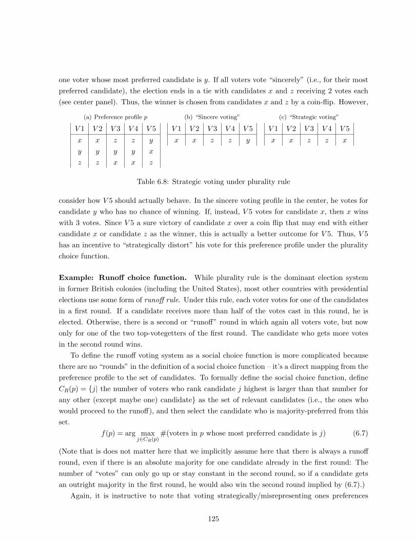
one voter whose most preferred candidate is y. If all voters vote “sincerely” (i.e., for their most

preferred candidate), the election ends in a tie with candidates x and z receiving 2 votes each

(see center panel). Thus, the winner is chosen from candidates x and z by a coin-flip. However,

(a) Preference profile p

V 1 V 2 V 3 V 4 V 5

x x z z y

y y y y x

z z x x z

(b) “Sincere voting”

V 1 V 2 V 3 V 4 V 5

x x z z y

(c) “Strategic voting”

V 1 V 2 V 3 V 4 V 5

x x z z x

Table 6.8: Strategic voting under plurality rule

consider how V 5 should actually behave. In the sincere voting profile in the center, he votes for

candidate y who has no chance of winning. If, instead, V 5 votes for candidate x, then x wins

with 3 votes. Since V 5 a sure victory of candidate x over a coin flip that may end with either

candidate x or candidate z as the winner, this is actually a better outcome for V 5. Thus, V 5

has an incentive to “strategically distort” his vote for this preference profile under the plurality

choice function.

Example: Runoff choice function. While plurality rule is the dominant election system

in former British colonies (including the United States), most other countries with presidential

elections use some form of runoff rule. Under this rule, each voter votes for one of the candidates

in a first round. If a candidate receives more than half of the votes cast in this round, he is

elected. Otherwise, there is a second or “runoff” round in which again all voters vote, but now

only for one of the two top-votegetters of the first round. The candidate who gets more votes

in the second round wins.

To define the runoff voting system as a social choice function is more complicated because

there are no “rounds” in the definition of a social choice function – it’s a direct mapping from the

preference profile to the set of candidates. To formally define the social choice function, define

CR(p) = {j| the number of voters who rank candidate j highest is larger than that number for

any other (except maybe one) candidate} as the set of relevant candidates (i.e., the ones who

would proceed to the runoff), and then select the candidate who is majority-preferred from this

set.

f(p) = arg maxj∈CR(p)

#(voters in p whose most preferred candidate is j) (6.7)

(Note that is does not matter here that we implicitly assume here that there is always a runoff

round, even if there is an absolute majority for one candidate already in the first round: The

number of “votes” can only go up or stay constant in the second round, so if a candidate gets

an outright majority in the first round, he would also win the second round implied by (6.7).)

Again, it is instructive to note that voting strategically/misrepresenting ones preferences

125

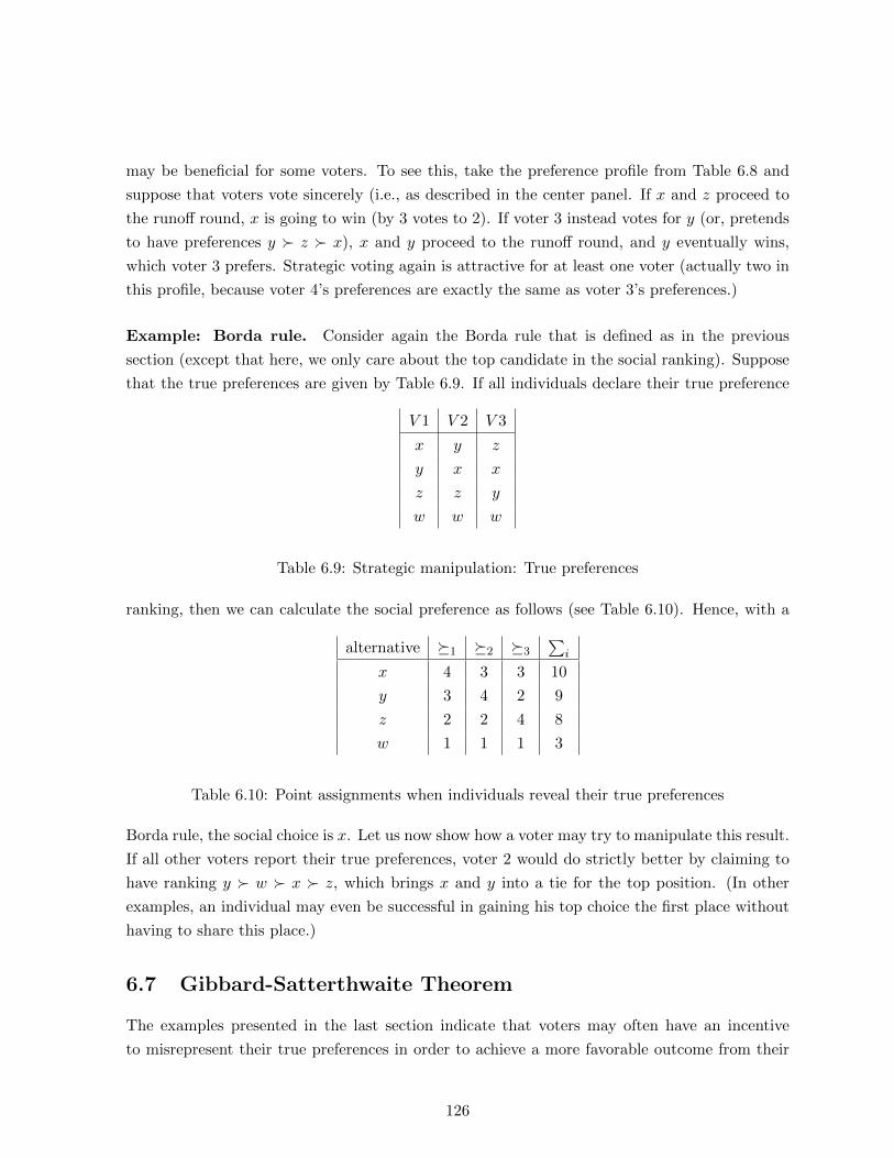
may be beneficial for some voters. To see this, take the preference profile from Table 6.8 and

suppose that voters vote sincerely (i.e., as described in the center panel. If x and z proceed to

the runoff round, x is going to win (by 3 votes to 2). If voter 3 instead votes for y (or, pretends

to have preferences y � z � x), x and y proceed to the runoff round, and y eventually wins,

which voter 3 prefers. Strategic voting again is attractive for at least one voter (actually two in

this profile, because voter 4’s preferences are exactly the same as voter 3’s preferences.)

Example: Borda rule. Consider again the Borda rule that is defined as in the previous

section (except that here, we only care about the top candidate in the social ranking). Suppose

that the true preferences are given by Table 6.9. If all individuals declare their true preference

V 1 V 2 V 3

x y z

y x x

z z y

w w w

Table 6.9: Strategic manipulation: True preferences

ranking, then we can calculate the social preference as follows (see Table 6.10). Hence, with a

alternative �1 �2 �3∑

i

x 4 3 3 10

y 3 4 2 9

z 2 2 4 8

w 1 1 1 3

Table 6.10: Point assignments when individuals reveal their true preferences

Borda rule, the social choice is x. Let us now show how a voter may try to manipulate this result.

If all other voters report their true preferences, voter 2 would do strictly better by claiming to

have ranking y � w � x � z, which brings x and y into a tie for the top position. (In other

examples, an individual may even be successful in gaining his top choice the first place without

having to share this place.)

6.7 Gibbard-Satterthwaite Theorem

The examples presented in the last section indicate that voters may often have an incentive

to misrepresent their true preferences in order to achieve a more favorable outcome from their

126

point of view. The question that we deal with in this section is whether there are any social

choice functions that do not suffer from this problem.

The answer to this question is yes, but only in a trivial sense: Consider, first, the social

choice function that always selects the same candidate (say, candidate x), no matter what the

preferences of voters are. Under this social choice function, there is clearly no incentive for any

voter to misrepresent his preferences (because candidate x is always selected, independent of

the voters’ preferences). Of course, this is not a particularly reasonable social choice function,

because it selects candidate x even if all voters dislike x.

Second, consider the social choice function that always selects the candidate who is most

preferred by voter d (our dictator from the last section). Clearly, voter d can only do worse if he

were to misrepresent his preferences, and since the other voters’ preferences do not count at all,

they also cannot gain from misrepresenting their preferences. The question is whether there are

more meaningful social choice functions that are also strategy-proof. This is the core question of

the Gibbard-Satterthwaite Theorem, that shows that the answer is negative.

In order to define strategy-proofness, it is useful to denote by pi the preference ranking of

voter i in preference profile p. Furthermore, let p−i be the preferences of everybody else.

Strategy-proofness means that, whenever f(pi, p−i) 6= f(pi, p−i), then f(pi, p−i) �i f(pi, p−i),

for all pi, p−i, pi. This has the following interpretation: pi is voter i’s “true” preference ranking,

while pi is a different ranking that voter i could pretend to have. If f(pi, p−i) 6= f(pi, p−i), then

voter i can change the social choice by reporting pi instead of the true preferences pi. If voter i

likes f(pi, p−i) (i.e., what he gets after “lying” about his preferences) better than what he gets

if he tells the truth, he will simply lie – for a mechanism to be strategy-proof, we require that

such a situation not arise (ever, that is for all possible true preference profiles).

In addition, the social choice function should satisfy Pareto optimality: If in preference profile

p every voter ranks candidate x highest, then f(p) = x. This is again a very mild requirement

– it imposes restrictions on social choice functions only if all voters agree on a preferred choice.

Nevertheless, this requirement excludes a constant social choice function such as in the example

above where a particular candidate is chosen no matter what preferences the voters have, and

that are therefore trivially strategy-proof.

Gibbard-Satterthwaite Theorem. If f is strategy-proof and Pareto-optimal, then f is dic-

tatorial: There is an individual d such that the social choice function always picks the most

preferred choice of individual d, no matter what preferences the other individuals in the society

have.

Conversely, no democratic aggregation mechanism is strategy-proof.

(proof to be written)

Interpretation. Just like with Arrow’s Theorem, it would be inappropriate to interpret the

Gibbard and Satterthwaite Theorem in the sense that it shows that “we need a dictator in order

127

to prevent strategic manipulation by voters.” Rather, the implication is that we should never

presume that voters (or legislators, for that matter) are simply automatons who will just blindly

report their true preferences if we just design the institutions appropriately; instead, in any

institutional setting, voters need to be considered as strategic agents.

128

Chapter 7

Direct democracy and the median

voter theorem

7.1 Introduction

In this chapter, we will move away from social choice theory and more towards a theory of

the political system which will eventually be occupied by strategically interacting voters and

politicians. This is the area that is called formal modeling by political scientists and political

economy by economists. Early in the history of economics, the entire discipline of economics was

called “political economy.” For example, one of the first and still leading journals in economics

is called the “Journal of Political Economy”. Today, there are also some people who use the

expression “political economy” when they mean “economics without using mathematics” (just

as they did in the good old days...). It is therefore useful to describe “political economy” as

understood here as “game-theoretic modeling of political processes”.

In this chapter, the political institutions are still very simple, as citizens vote directly on

policy. We present a simple framework with one-dimensional policy and structured voter pref-

erences, introduced by Anthony Downs, that is sometimes called the spatial model, the median

voter model and sometimes just the Downsian model. This model has a very simple equilib-

rium and is by far the most popular model when economists from other areas want to add some

political features to their model.

7.2 Single-peaked preferences

The completeness axiom in Arrow’s theorem requires that the preference aggregation mechanism

return a social preference ranking for all possible preferences of voters. We have seen in the last

chapter that there exist some voter preference profiles for which simple majority preference is

intransitive.

129

In an environment without any structure, this requirement appears necessary, as it is difficult

to exclude certain voter preferences a priori. However, the political or economic environment

sometimes provides us with insights as to which type of preferences we can expect. When

we restrict the class of voter preferences, simple majority preference may be transitive (on

the smaller class of admissible preference profiles). For example, this is obviously the case if

we restrict our attention to preference profiles in which all voters agree on the ranking of all

alternatives. Of course, that would not be a particularly relevant class as it is rarely the case

that all voters agree. Therefore, the class of admissible voter preferences should still be large

and empirically important.

Fortunately, many political issues have a certain structure that restricts reasonable prefer-

ences in a particular way. For example, consider the issue of voting on tax rates and implied

public spending. A community has to choose a proportional tax rate (say, for a sales tax) and

uses the proceeds to buy some public good. Of course, nobody likes to pay taxes, but all people

like public goods (some more so than others), and since every level of taxes relates to a level

of spending on public goods, we can just consider preferences over tax rates, and individuals’

“most preferred tax rates” will generally be positive.

Suppose, for example, that 25% is the current status quo tax rate. It would appear unlikely

that an individual prefers both 30% and 20% over 25%. It is plausible that an individual wants

lower taxes (and is willing to accept the accompanying reduction in public services); it is also

plausible that an individual would like to have more public services and is willing to accept

higher taxes in return. However, an individual who prefers both 30% and 20% over 25% would

essentially not take a “taxes are too high” or a “taxes are too low” standpoint, but just say

that he wants a different tax rate, no matter whether it is higher or lower. That is not a very

plausible preference, and it will be the type of preference we exclude from admissible preferences

in this chapter.

We assume that individual preferences over tax rates τ are “single peaked” with convex better

sets (see Figure 7.1). For example, an individual whose most preferred tax rate (his bliss point)

is 20% would likely prefer a tax rate of 25% over a tax rate of 30%, and a tax rate of 15% over

one of 10%.

Note that we don’t require that an individual with a preferred tax rate of 20 percent be

indifferent between tax rates of 15% and 25%, just because these tax rates have the same

“distance” from his most preferred point. It is quite conceivable that the utility function is

asymmetric around the most preferred point so that the individual above prefers 15% to 25%

or vice versa, and therefore we do not make any assumptions related to options that are on

different sides of the bliss point. Single-peakedness only requires that coming closer to the bliss

point without passing to the other side increases an individual’s utility.

When the vote is on tax rates, there is a natural ordering of proposals, namely according

to the size of the tax rate. For other applications, say, voting for one of several candidates for

130

-

6

0

τ

ui(τ)

Figure 7.1: Single-peaked preferences

president, there is not necessarily such a “natural” ordering.1 Assuming that individuals have

strict preferences over candidates, any individual’s preferences can be made “single-peaked”

by appropriately re-labeling the choices. However, for the results that we develop below to

hold in such a setting, it has to be true that there is an ordering of alternatives that produces

single-peakedness and is the same for all voters.

7.3 Median voter theorem

7.3.1 Statement of the theorem

If all individuals have single-peaked preferences relative to the same ordering of alternatives,

then there is a unique candidate who beats all other candidates in a pairwise election. Such a

candidate is called a Condorcet winner.

Definition 5. A Condorcet winner is a proposal that is preferred to any other proposal by a

majority of the electorate.

The following theorem was first stated by Duncan Black in 1948.

1It may be possible that we can rank the candidates from “left” to “right” and all voters care only about this

dimension, but this is not necessarily guaranteed.

131

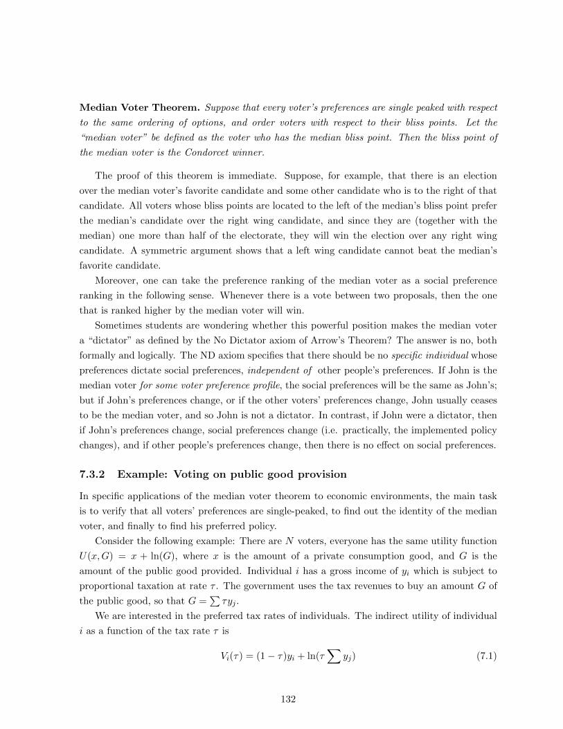
Median Voter Theorem. Suppose that every voter’s preferences are single peaked with respect

to the same ordering of options, and order voters with respect to their bliss points. Let the

“median voter” be defined as the voter who has the median bliss point. Then the bliss point of

the median voter is the Condorcet winner.

The proof of this theorem is immediate. Suppose, for example, that there is an election

over the median voter’s favorite candidate and some other candidate who is to the right of that

candidate. All voters whose bliss points are located to the left of the median’s bliss point prefer

the median’s candidate over the right wing candidate, and since they are (together with the

median) one more than half of the electorate, they will win the election over any right wing

candidate. A symmetric argument shows that a left wing candidate cannot beat the median’s

favorite candidate.

Moreover, one can take the preference ranking of the median voter as a social preference

ranking in the following sense. Whenever there is a vote between two proposals, then the one

that is ranked higher by the median voter will win.

Sometimes students are wondering whether this powerful position makes the median voter

a “dictator” as defined by the No Dictator axiom of Arrow’s Theorem? The answer is no, both

formally and logically. The ND axiom specifies that there should be no specific individual whose

preferences dictate social preferences, independent of other people’s preferences. If John is the

median voter for some voter preference profile, the social preferences will be the same as John’s;

but if John’s preferences change, or if the other voters’ preferences change, John usually ceases

to be the median voter, and so John is not a dictator. In contrast, if John were a dictator, then

if John’s preferences change, social preferences change (i.e. practically, the implemented policy

changes), and if other people’s preferences change, then there is no effect on social preferences.

7.3.2 Example: Voting on public good provision

In specific applications of the median voter theorem to economic environments, the main task

is to verify that all voters’ preferences are single-peaked, to find out the identity of the median

voter, and finally to find his preferred policy.

Consider the following example: There are N voters, everyone has the same utility function

U(x,G) = x + ln(G), where x is the amount of a private consumption good, and G is the

amount of the public good provided. Individual i has a gross income of yi which is subject to

proportional taxation at rate τ . The government uses the tax revenues to buy an amount G of

the public good, so that G =∑τyj .

We are interested in the preferred tax rates of individuals. The indirect utility of individual

i as a function of the tax rate τ is

Vi(τ) = (1− τ)yi + ln(τ∑

yj) (7.1)

132

In order to find the optimal tax rate for individual i, we take the derivative of (7.1) to get

−yi +1

τ= 0 (7.2)

Differentiating the derivative a second time gives −1/τ2 < 0 so that i’s indirect utility is globally

concave in τ and therefore in fact has a single peak.2 Solving (7.2) for τ yields τ∗i = 1yi

. This

shows that richer voters prefer a smaller tax rate, so voter bliss points are ordered with respect

to the individuals’ initial incomes. The median rich individual with initial income ym is the

median voter and thus determines the equilibrium tax rate, so that we get τcw = 1/ym as the

Condorcet winner. Any higher tax rate is defeated because the richer half of the electorate plus

the median voter prefer τcw over any higher tax rate. Similarly, any lower tax rate is defeated

because the poorer half of the electorate plus the median voter prefer τcw over any lower tax

rate.

It is interesting to ask how this Condorcet winner tax rate, which we interpret as the equi-

librium outcome in this democratic society, compares to what is “socially optimal”. To do this,

we first need to think about what we mean by “socially optimal.” The standard concept of

optimality in economics is Pareto optimality: If it is not possible to make some voter better off

without harming some other voter, then a policy is Pareto optimal.

Applying this concept to our setting here, we have a wide range of Pareto optimal policies:

All tax rates that are not below the ideal tax rate of the voter with the lowest bliss point, and

not above the ideal tax rate of the voter with the highest bliss point are Pareto optimal. To

see this, consider a tax rate that is strictly in between the highest and the lowest bliss point.

Then, the voter with the lowest bliss point dislikes all increases in the tax rate, and the voter

with the highest bliss point dislikes all decreases in the tax rate – thus, there are no policy

changes on which these two voters could agree, and so any change will make some voters worse

off. Therefore, the initial starting point is Pareto optimal.

In contrast, consider a tax rate that is below even the bliss point of the voter with the

lowest bliss point. In this case, every voter agrees that some small increase (at least up to the

lowest bliss point) is desirable. Thus, the initial tax rate was not Pareto optimal. An analogous

argument shows that a tax rate above the bliss point of the voter with the highest bliss point is

not Pareto optimal.

Thus, the Condorcet winner is Pareto optimal, but it is only one of very many Pareto optimal

policies. In general, the concept of Pareto optimality has very little bite in political settings (i.e.,

under most conceivable institutions, policies will be Pareto optimal in equilibrium). For example,

note that dictatorships (in the sense of Arrow) result is Pareto optimal policies because the policy

chosen is the one that maximizes the utility of the dictator. Thus, many Pareto optimal policies

are not really “socially optimal” in any meaningful way; they may benefit a tiny minority slightly

2Note that concavity of the indirect utility function in τ is sufficient, but not necessary for single-peakedness.

The necessary and sufficient condition is that the indirect utility function be quasiconcave in τ .

133

while substantially harming a large majority of the electorate.

One possibility is to just interpret the concept of a Condorcet winner as a normative concept:

The objective of the institution of democracy is to implement the “wishes of the population.”

Since citizens do not always agree on policy, it is best to implement the policy that is preferred

by a majority of citizens.

Another approach is called “utilitarianism,” in which the objective is to maximize the sum

of all voters’ utilities. This approach goes back to Jeremy Bentham, a 19th century English

philosopher who said that the objective of government should be to achieve “the largest utility

for the largest number of people.” Clearly, this is not a well-defined mathematical objective

function, and one could reasonably argue that it actually sounds like a normative endorsement

of the Condorcet winner, in the sense that there is no other policy that leads to a larger utility for

a majority of voters than the Condorcet winning policy. However, the way that utilitarianism

has been operationalized traditionally is as a maximization of the sum of all voters’ utility

functions.

From the point of view of economic theory, aggregating the utility of different voters is some-

what problematic, as we know from microeconomics that utility functions are defined only up

to an ordinal transformation. For example, we can simply multiply voter 1’s utility function by

85 (say), and the new utility function reflects exactly the same preferences as the original one.

However, voter 1 is one of the voters whose utility enters the utilitarian objective function, and

multiplying his utility leads to a change in the policy that maximizes the utilitarian objective

(i.e., the new utilitarian objective function now puts a much larger emphasis on voter 1’s prefer-

ences, a change which is equivalent to adding 84 people who have exactly the same preferences

as voter 1 in the initial scenario.

Thus, for the utilitarian approach to make sense, the utility functions need to be comparable

across voters so that it makes sense to sum them up. One possibility is to use utility functions

in which policy preferences are expressed in “money-metric” terms, that is, the utility function

measures how much of the private good an individual would be willing to give up in order to

receive a more favorable policy. In our application here, the utility functions satisfy this criterion

of comparability because one dollar given to any voter increases this voter’s utility by exactly

one unit (through consumption of the private good). Maximizing the utilitarian utility function

max[

N∑i=1

(1− τ)yi] +N ln(τ∑

yj) (7.3)

by choosing the tax rate τ gives the following first order condition:

−Y +N1

τ= 0, (7.4)

where Y ≡∑yi is the total income of all citizens. Hence, the utilitarian optimal tax rate is

τSO = 1y , where y = Y/N is the average income.

134

How does this tax rate compare to 1/ym? Empirically, the average income in society is always

higher than the median income. The reason is that there are a number of very rich individuals

whose incomes raise the average income a lot, but hardly at all change the median income. In

contrast, low income is usually bounded at 0. If we take ym < y as given, then τ > τSO and

G > GSO, so that the utilitarian optimum would be to reach at a lower tax level (and a lower

level o provision of the public good).

The intuitive reason is that the median voter gets a share of 1/N of the total benefit from the

public good (since all individuals receive the same benefit), but pays less than 1/N of the total

taxes, because his median income is less than the average income. This provides an incentive

to overspend for the median voter. Moreover, this effect is the bigger, the larger the difference

between mean and median income is; in general, we would expect more unequal societies (with

respect to initial income) to have a larger gap between median and mean income, and they should

therefore tend to have higher tax rates than societies that are initially more equal. Interestingly,

this robust prediction of the model appears to be refuted by empirical evidence which suggests

that more unequal societies actually have lower tax rates than more equal societies.

While the utilitarian way of aggregating utility across voters is perhaps attractive because

it allows us a clearer benchmark than the concept of Pareto optimality, it must be emphasized

that the approach is based on a particular value judgment, namely that individuals’ willingness

to pay for a policy is the basis according to which we should judge whether a policy is efficient.

If policy preferences are a normal good, then richer people are more willing to pay for their

favorite policy.

For example, consider a Presidential election with just two candidates. Utilitarianists would

measure each voter’s net willingness to pay for a victory of candidate A (i.e., this measure is

positive if an individual wants A to win, and negative if he wants B to win), and argue that

a victory of A is efficient if and only if the aggregate sum of these net willingness to pay is

positive. Suppose that the victory of one’s favorite candidate in the Presidential election is a

normal good, so that richer people would be, at least on average, willing to pay more for a

victory than poor people (this appears quite reasonable). In this case, rich voters matter more

for who the “utilitarian optimal” candidate is than poor voters. For example, if 52 percent

of voters prefer candidate B, but the average willingness to pay of A-supporters is sufficiently

larger, then an electoral victory of B would be classified by utilitarians as inefficient, but this is

clearly a value judgment (i.e., one can agree or disagree with this approach).

7.4 Multidimensionality and the median voter theorem

The median voter theorem is often interpreted in the sense that for “realistic” preferences, the

potential problems indicated by Arrow’s impossibility theorem do not exist. For single peaked

preferences, a Condorcet winner exists. However, this is an incorrect interpretation because the

135

median voter theorem does not carry over to the case that there are several dimensions of policy,

even if preferences in this policy space are still single-peaked.

As an example of a multidimensional policy space, consider the following simple example.

Suppose there are three interrelated decisions: How much taxes to raise, and how much to

spend on welfare programs supporting the poor, and how much to spend on defense. Since

the sum of expenditures for both types of programs must equal the taxes raised, we know the

third component if we are given two of these choices, and therefore we can graph preferences

in a two-dimensional graph featuring taxes on the horizontal axis and defense spending on the

vertical axis. See Figure 7.2.

6

-

defense

taxes

•1

•x∗

3

•4

•2

•5

Figure 7.2: Multidimensional bliss points, radially symmetric around x∗

The dots in the graph are the ideal positions of the different voters whose number is next to

the point. For example, voter 1 is for low taxes and low defense spending. A natural conjecture

extending the one-dimensional median voter theorem is that the “most central voter” (perhaps

the median in each direction) should again be decisive. However, generically, no Condorcet win-

ner exists if the issue space is multidimensional, even if all voters have single peaked preferences.

“Generically” here means “in almost all cases, except for very special parameter cases”. This

result is due to two papers by McKelvey and Plott in the 1960s/70s.

Plott-McKelvey Theorem. Suppose that there are multiple policy dimensions and that all

voters’ preferences are single-peaked and Euclidean (i.e., indifference curves are circles around

the respective bliss points). A Condorcet winner x∗ exists in a multidimensional setting, if and

only if the voters’ bliss points are radially symmetric around x∗.

136

Figure 7.2 can be used to illustrate the Plott-McKelvey theorem. The points in the graph

are the bliss points of the five different voters. Assume that each voter has indifference curves

that are circles, i.e. voters evaluate policies according to the distance to their bliss point (this

is not essential for the result, but it makes the discussion simpler). The bliss point of voter 3,

x∗, is the “median in every direction”. That is, any line through another voter’s bliss point and

x∗ contains also the bliss point of a third voter, and x∗ is in between the two other voters bliss

points.

The first claim of the theorem is that x∗ is the Condorcet winner. To see this, consider the

vote between x∗ and some other policy y, which is not necessarily the bliss point of another voter

(see Figure 7.3). Voters whose bliss point is on the line in the graph are indifferent between x∗

and y. The line intersects the line that connects x∗ and y at its midpoint and at a 90 degree

angle. Those voters whose bliss point is below the line prefer x∗ to y, and those whose bliss

point is above it prefer y to x∗.

6

-

defense

taxes

•x∗

3

•y

@@@@@@@@@@@@@@

Figure 7.3: Vote between x∗ and y

If voters bliss points are radially symmetric around x∗, then, for any y 6= x∗ there are always

more voters with bliss points in the x∗-halfplane than those with bliss points in the y-halfplane.

Hence, no other policy y wins a majority against x∗.

However, it is extremely unlikely that the voters’ preferences satisfy the radial-symmetry

condition in the real world, and if the condition is not satisfied, no Condorcet winner exists.

To see this, note first that, if a Condorcet winner exists, it must be one voter’s ideal point. To

see this, note that all lines that go through a point that is not a voter’s ideal point and avoid

touching any voter’s ideal point (that is true for almost all lines that ne can draw) will separate

137

a strict majority of people from a minority, and, by the same argument as above, policies that

are a little inside the half space and on the normal are preferred by a majority to the initial

point.

Second, consider a point that is one voter’s ideal point (say, x∗). Even in this case, separating

a majority from a minority is usually possible. To see this, draw a line through this point. If

there are N−12 voters on each side, then start to rotate the line around x∗, say, in a clock-wise

direction. After some rotation the upper half-plane either loses or gains an additional voter,

and then, there is a strict majority in one half plane. The only exception to this is if the upper

half-plane simultaneously wins and loses one voter (which happens if there are two voters who

are directly opposite from each other, at different sides of x∗. In this case, keep rotating the line

until you either get the first strict majority in a half-plane. Only if you can complete a full 360

degrees rotation without ever getting a strict majority in one half-space – and this is true only

if all voter ideal points are radially symmetric around x∗ –, then x∗ is the Condorcet winner.

What happens when voter ideal points are not radially symmetric so that no Condorcet

winner exists? A interesting question to ask when no Condorcet winner exists is the following:

Is there a set of policies such that all policies in the set are preferred by majority to any point

outside the set? This set is called the top cycle. If a “small” top cycle exists, the non-existence

of a Condorcet winner is not quite so bad — we don’t know which element of the top cycle is

going to be selected as policy in a democratic society (because there is no Condorcet winner, all

policies “can be beaten” by some other policy), but at least we also know that policies outside

the top cycle are unlikely to arise, since a majority prefers any policy in the top cycle to it.

Unfortunately, in the model with spatial voter preferences, the top cycle if really large (unless

we are in the perfectly radially-symmetric setting, in which a Condorcet winner exists). In fact,

we show that the following is always possible if bliss points are not radially symmetric: Pick

any two policies x and y, such that a majority prefers x to y (those do not have to be bliss

points of any voters, just any policies). Then we can find a sequence z1, z2, . . . , zn such that z1

is majority preferred to x, z2 is majority preferred to z1, . . . and y is majority preferred to zn.

Thus, starting from policy x, we can reach the point y through a sequence of “majority votes”,

even though we know that the initial point x is majority-preferred to x.

To see how this can be done, consider the following Figure 7.4. The dots correspond to

the ideal points of the three voters, and the small crosses are the policies. Note first that both

voters 2 and 3 clearly prefer policy x to y. Policy z1 is slightly closer for both voter 1 and 2

than policy x (and is thus preferred to x by them). To see this, note that z1 is constructed by

mirroring x on the line that connects the ideal points of voter 1 and 2 (and moving it back a

little closer to the line).

Similarly, policy z2 is constructed by mirroring z1 at the line that connects voter 1 and

voter 3 (and again, moving a little closer back to the line). Thus, a majority (this time, voters

1 and 3) prefer z2 to z1. Finally, it is obvious that y is closer to the ideal points of voters 1

138

6

-

x1

x2

•1

•3

•2

x ×

y×

z1×

z2×

Figure 7.4: Getting from x to y through majority votes

and 2 (and maybe even 3) than z2. Thus, a majority of voters prefers y to z2, and we get the

following intransitive majority preference chain: y � z2 � z1 � x � y.

Note that x and y can be chosen completely arbitrarily. As long as the three voter ideal

points span a triangle (i.e., they are not radially symmetric), the same type of construction can

be used to get a sequence of zi that are all majority preferred relative to the previous policy, but

move farther and farther away from the center, so that eventually y is majority-preferred to zn.

139

Chapter 8

Candidate competition

8.1 Introduction

In reality, there are few societies in which voters decide directly on policy. In most cases, voters

rather elect a politician who will then choose policy. In parliamentary systems, influence is

often even more indirect, in that voters vote for one of many politicians who form a legislature

and who (in addition to voting on legislation) vote for the government that implements policy.

While voters have therefore only indirect influence, the question of which policy is going to be

implemented is of course front and center during the election campaign.

The fundamental notion that competition is beneficial carries over from the economic field

to the one of politics. It appears very likely that a candidate who is in fierce competition with a

competitor and who has to fear that voters might elect his rival will behave better — in terms

of effort, in terms of not choosing blatantly self-serving actions, and in terms of choosing policy

that reflects the preferences of his constituents — than a candidate who is assured of victory

and can effectively behave like a political monopolist. However, to study this idea in more detail

requires that we develop explicit models in which candidates compete for office.

We will present a number of such models have been developed. However, before we do this, it

is useful to summarize the main questions that all of these models aim to provide some insights

into. This will help us to grasp what we learn from each of the different models.

Explain policy convergence or divergence? Are the positions that candidates take in real-

life campaigns “surprisingly similar” or “surprisingly different”? To paraphrase, do candidates

offer voters “a real and clear choice between two different political philosophies”, or do they

most often just offer two flavors of essentially the same policy? Of course, there are always some

differences between candidates’ positions, so the answer to our question depends on whether

we would expect larger or smaller differences than we observe. Moreover, the degree of policy

convergence or divergence may also differ between different election campaigns, and, even in one

election campaign, candidates will usually differ in their proposed policy in some policy areas,

140

while advocating the same policy in other areas. The follow-up question is, of course, which

exogenous factors are responsible for the difference between political campaigns, and between

different policy areas.

Incentives to converge. When candidates choose platforms, which incentives influence their

choice? A candidate might care about winning office, and he might genuinely care about the

policy that is implemented (either by himself, in case that he wins, or otherwise by his opponent).

What are the trade-offs that determine whether it is better for a candidate to propose more or

less similar policies to those of his opponent? In reality, both the desire to win (office motivation)

and the desire to influence policy (policy motivation) will influence candidates to a certain extent.

Can we learn from candidate behavior which of these motivations is more important for them?

Candidate differences and their effect on position choice In reality, candidates differ in

some exogenous aspects — for example, a candidate’s previous history determines, to a certain

extent, important aspects of how he is going to be perceived by the electorate. Incumbents

may have an advantage in that they have already learned tasks on the job and are thus more

productive than challengers who would first have to acquire similar knowledge in office if elected.

Do these differences in quality and/or productivity affect where candidates optimally locate in

the policy space?

Is political competition efficient? Is there too much or too little convergence? Is the

degree of policy convergence or divergence that we see good or bad for voters? Is more “bipar-

tisanship” and “moderation” what would be needed in Washington (and around the country)?

This would be the case if the equilibrium behavior of candidates is excessively polarized. On

the other hand, it could also be the case that equilibrium policy choices are excessively similar,

and it would then be desirable to have clearer contrasts between parties so that “elections mat-

ter”? Depending on the model, the answers to these questions differ, and so it is important to

both understand which effects drive the different results in different models, and to be able to

distinguish the models empirically.

While we will mostly deal with candidate competition in the plurality system, it is evident

that the question of how efficient the equilibrium of political competition is, is particularly

relevant when comparing the performance of different electoral systems: Is proportional repre-

sentation or runoff rule better or worse for voters than plurality rule?1

1This question is rarely analyzed and far from settled in the theoretical literature, and so we will not be able

to provide an answer here. However, it is ultimately one of the most interesting ones in this research area.

141

8.2 The Downsian model of office-motivated candidates

The simplest model of candidate competition goes back to the setting of the median voter

theorem. There is a one-dimensional policy space, and all voters have single-peaked preferences

in this space. Candidates know the preference profile (i.e., the distribution of voters’ ideal

points), and choose their position in order to maximize their respective probability of winning

the election. Trust is not an issue in this simple model: Candidates are assumed to be able to

commit to a position, so that all voters trust that they will implement exactly this position if

they are elected. Voters do not care about the identity (personality, competence) of candidates,

but only about their announced policy positions. Finally, voters who are indifferent between

two or more candidates decide randomly whom to vote for.

Clearly, if there are two candidates who choose their positions simultaneously, then there is a

unique Nash equilibrium in which both candidates choose a position equal to the median voter’s

ideal position. As we have seen in Chapter 7, with single-peaked preferences, the median voter’s

preferences are decisive for which of two positions gets a majority, because either everybody “to

the left” of the median voter votes the same way as the median, or everybody to the right of

the median voter does – in either case, this is a majority for the candidate who is supported by

the median voter.

Thus, choosing the position that maximizes the utility of the median voter is a weakly

dominant strategy: A candidate who adopts it will win outright if the other candidate adopts

a different position, and will have a 50 percent winning probability if the other candidate also

adopts the median voter’s favorite position (but in that case, any other position would lose

against the opponent). So, no matter what the opponent chooses, adopting the median voter’s

preferred position is an optimal action for a candidate in this game.

This result is very robust to several variations of the game as long as there are two candidates.

However, things change potentially when there are three or more candidates. We now go through

some possible variations of the game.

Timing of actions. The basic model of Downsian competition assumes that candidates moves

simultaneously when deciding on their position. However, it would not matter if candidate A

was the first to choose his position, while candidate B can observe A’s choice and then choose

his own position. To see this, note that B’s optimal response, no matter what position A chose,

is to pick the median voter’s bliss point. The only action that leaves A with some chance of

winning the election is to choose the median voter’s bliss point as well.

Policy motivated candidates The basic model assumes that candidates care only about

winning, not about the policy that they have to implement. What would change if candidates

care (only) about the eventually implemented policy?

142

Suppose that the Democrat has a utility function of uD(x) = −(x+ 1)2 and the republican

has a utility function of uR(x) = −(x − 1)2. That is, both candidates have single-peaked,

distance-based policy preferences, and the Democrat’s bliss point is at θD = −1, while the

Republican’s ideal policy is at θR = 1. Suppose furthermore that the median voter has an ideal

policy of θM = 0, i.e., a utility function of uM (x) = −(x− 0)2 = −x2.In this case, both candidates would like to move away from 0 in the direction of their ideal

policy. However, if a candidate does just that, he will lose for sure as long as the other candidate

remains at 0. Thus, (0, 0) remains a Nash equilibrium of the game between the candidates. (Note

that candidates in this variation do not mind losing per se; but, if a candidate loses, then he

also does not benefit from moving his platform closer to his ideal point).

Also, one can check that there is no other Nash equilibrium. Clearly, (−a, a), that is,

both candidates locating a distance a away from the median voter, is not an equilibrium – a

candidate could move slightly closer to the median and win for sure, rather than with probability

1/2; this increases the candidate’s expected utility from policy. For example, this deviation

would give the Republican a utility of uR = −(1 − a − ε)2 rather than the expected utility of

uD = −12(1− a)2 − 1

2(1− (−a))2 that he gets if he sticks to position a. For ε sufficiently small,

the deviation is beneficial. Also, (−a, b) with b 6= a (i.e., both candidates propose non-median

policies, but one of them is closer to the median and therefore wins for sure) is not an equilibrium

– the loser can simply deviate to a position that is slightly closer to the median than the winner’s

position, and be better off. Finally, consider the profile (0, b) with b > 0 so that the Democrat

wins. If the Democrat becomes a little bit more radical in this case, we would still win but

receive a higher utility, so that this profile is not an equilibrium, either.

Note that, formally, this game is very similar to the classical Bertrand competition game

in which two firms with the same constant marginal costs choose which price to charge, and

all consumers choose to buy from the firm that charges the lower price. In this game, firms

would like to charge a price larger than their marginal cost, but competitive pressure moves the

equilibrium price all the way down to marginal costs. The same type of argument implies that,

while the parties would like to propose more extreme policies, competitive pressure from the

other party prevents them from doing so.

Uncertainty about the preference distribution. We now return to the assumption that

candidates are office-motivated, but assume that the bliss point of the median voter is unknown.

The way to model such uncertainty is to assume that, from the candidates’ point of view, the

median’s bliss point is a random variable drawn from some distribution. For concreteness,

suppose that this distribution is uniform on the interval [−0.5, 0.5]. Note that the cumulative

distribution function of this uniform distribution is FM (x) = x+ 0.5 (for x ∈ [−0.5, 0.5], and is

143

truncated to 0 or 1 outside this interval, respectively).2

Denote the Democrat’s position by xD and the Republican’s position by xR. If the two

candidates choose different positions with xD < xR, then only one voter type is indifferent

between these positions, and that is the voter whose ideal policy is xD+xR2 . Whenever the

realized median voter happens to be to the left of this value, which happens with probability

FM(xD+xR

2

), then the Democrat wins, and otherwise the Republican wins.

If xD = xR, i.e. both candidates choose the same position, then all voters are indifferent

between the candidates and consequently both win with probability 1/2. Note that it is irrelevant

for this result what the bliss point of the realized median voter is.

Finally, if the two candidates choose different positions with xD > xR,3 then we have the

mirror image of the first case. The indifferent voter type is again xD+xR2 , and whenever the

realized median voter happens to be to the right of this value, which happens with probability

1− FM(xD+xR

2

), then the Democrat wins, and otherwise the Republican wins.

Fix a value of xR. What is the optimal action that the Democrat should take to maximize

his winning probability? There are three potentially attractive positions. As long as xD < xR,

the Democrat’s winning probability is increasing in xD, so the Democrat wants to go as close

as possible to xR (without actually reaching it). This strategy gives (approximately) a winning

probability of FM (xR) because the Democrat wins whenever the realized median is to the left

of xR.

Alternatively, the Democrat could choose a position to the right of xR; as long as he does

that, his winning probability is decreasing in his own position, so he optimally chooses xD is

close as possible to xR (without actually reaching it), which gives him a probability of winning

of approximately of 1−FM (xR) because the Democrat wins whenever the realized median is to

the right of xR.

Finally, if the Democrat chooses the same position as the Republican, both candidates win

with probability 1/2. Thus, the Democrat’s optimal action is to choose the best of these three

actions, which allows him to achieve a winning probability of max(FM (xR), 12 , 1− FM (xR)

).

Note that this is always greater or equal to 1/2 (because “1/2” is one of the terms in the

brackets, and if FM (xR) = 1/2, then all terms in the bracket take the value 1/2).

Since the Republican’s winning probability is 1 minus the Democrat’s winning probability

(this is called a “constant-sum-game, because the two players’ payoffs, i.e.. winning probabilities

for all pirs of strategies sum to the same constant, 1), the Republican’s best action is to minimize

max(FM (xR), 12 , 1− FM (xR)

). Thus, he should choose xR such that FM (xR) = 1/2. That is,

he should choose the “median median,” that is, the median value of the distribution of possible

2Remember that the value of a distribution function at x, F (x) gives the probability that the value of the

random variable is less or equal to x.3Note that we do not exclude this constellation a priori – while our observations tell us that Democrats usually

have positions to the left of Republicans, it is important not to exclude the possibility of other constellations from

the get-go.

144

positions of the median voter.

The same argument holds for the Democrat. Thus, both candidates also choose the same

platform if the position of the median voter is uncertain. Specifically, they choose the “average”

position of the median voter (however, they go for the median rather than the expected value

of that random variable).

In summary, the assumption that there is uncertainty about the position of the median voter

does not fundamentally change the result of the median voter theorem. Candidates still choose

the same position, and it is as close to the median as the setting with uncertainty allows for. We

will return to the setting with uncertainty about the median voter’s preferred position below in

Section 8.3 where we will combine it with the assumption of policy-motivated candidates. We

will see that this combination of assumptions actually leads to some more substantive changes

in results.

Three or more candidates. What happens in the Downsian model if there are three or more

candidates? In order to analyze this situation, we need to first talk about how voters decide

whom to vote for if there are more than two candidates. With just two candidates, voters’

decision problem is really simple: Vote for the candidate who you prefer more because whenever

your vote makes a difference (in the sense of deciding who actually wins the election), you prefer

the outcome if you vote for your favorite candidate.

As we have seen in Chapter 6in the discussion of Table 6.8, this is not necessarily true if

there are three (or more) candidates. For voters whose preferred candidate has no chance of

winning, it is better to vote for one of the top contenders than for their own favorite. And, of

course, which candidates have any chance of winning depends on the strategies played by all

(other) voters. As a consequence, there are potentially many voting equilibria when there are

more than three candidates.

We will discuss this in more detail in Section 8.4 below. In this section, we want to assume

instead that all voters vote sincerely, that is, for their most favorite candidate (and that they

randomly distribute their vote if they are indifferent).

Consider what happens with three candidates who choose simultaneously. Denote the cumu-

lative distribution of voter ideal points by F (·), and assume that the median voter’s bliss point

is at 0 (so that F (0) = 1/2). There is no equilibrium in which all three candidates choose 0, the

median voter’s bliss point. To see this, note that deviating to ε (i.e., a little bit to the right),

if the two competitors are both at 0, wins the election: The candidate who deviates gets the

votes from all voters whose ideal point is to the right of the median (i.e., almost 50 percent of

the voters), while the two other candidates split those voters whose ideal points are to the left

of the median (and the median, too), which results in a vote share of approximately 25 percent

for both of the competitors. So, the deviator would win for sure, and thus the original strategy

profile in which all candidates locate at the median voter’s bliss point is not an equilibrium.

145

Second, consider a profile of positions (−a, a, a) for a not too big (we will specify what “not

too big” means precisely in a second). With these positions, the candidate at −a receives the

votes of all voters to the left of the median, while the two other candidates split the right half of

the electorate; thus, the candidate at −a wins. Can either of the two losing candidates deviate

and win (or at least tie for the first place)? The answer is negative. If a candidate moves to

a + ε, then his vote share is 1 − F (a) < 1 − F (0) = 1/2, so he loses. If the candidate deviates

to a point in x ∈ [−a, a], he receives the votes of types between (−a + x)/2 (i.e., the type who

is indifferent between the candidate at −a and the candidate who deviates) and (x+ a)/2 (i.e.,

the type who is indifferent between the candidate at a and the candidate who deviates). The

deviator’s vote share is thus F(x+a2

)−F

(x−a2

)< F (a)−F (−a). For a small enough, this is less

than F (−a), so that the deviator would still lose to the candidate at −a. Third, suppose the

deviator moves to some position x = −a so that he splits the votes of the previous winner; then

the candidate who remained at a wins with 1/2 of the votes, while the deviator and the winner

in the original strategy profile each get only one quarter of the votes. Finally, the deviator also

loses (to the candidate who remains at a if he moves to a position x < −a.

In summary, the only requirement for (−a, a, a) to be an equilibrium is that F(x+a2

)−

F(x−a2

)< max(F

(x−a2

), 1 − F

(x+a2

)so that a candidate who deviates to some point in the

middle between −a and a still loses.

Suppose, for example, that voter types are distributed uniformly on [−1, 1]. In this case,

F (t) = (1 + t)/2 is the cumulative distribution function of voter ideal points. Then

F

(x+ a

2

)− F

(x− a

2

)=

1 + x+a2

2−

1 + x−a2

2=a

2

is the vote share that a candidate who deviates to a policy x ∈ (−a, a) will receive (any deviation

will lead to the same vote share; that result depends on the voter distribution being uniform).

To minimize max(F(x−a2

), 1− F

(x+a2

), choose x = 0. This gives F (−a/2) = 1/2− a/4 as

the vote share of each of the two competitors. A deviation to 0 will not be sufficient to win ifa2 <

12 −

a4 , which simplifies to a < 2/3.

Of course, there is also a symmetric equilibrium in which two of the candidates locate at −aand only one at a, and the candidate at a wins the election. Furthermore, there are equilibria

in which the candidates locate at three different positions, to see this, take the equilibrium from

above, (−a, a, a), and move one of the two losing candidates slightly away from a. They will

still lose, and the candidate who remains at a also has no possibility to deviate and win4

However, it is important to note that, in no equilibrium, the median’s preferred position of

0 is proposed by the winner of the election. To see this, note first that we have already shown

that it cannot be true that all candidates locate at 0. Furthermore, if two candidates locate at

4For the other candidate, we already checked above that there is no other position where he could win, given

that his opponents are at −a and a.

146

zero, then the remaining candidate can win by adopting a policy slightly to the left (or right)

of zero.

Finally, can it be the case that only candidate 1 (say) locates at 0, and wins the election in

equilibrium? The answer is negative. Consider candidate 2: If he locates on the opposite side

of candidate 3 (the other competitor), but closer to 0, then he attracts more votes than either

candidate 1 or candidate 3, and he therefore wins the election. Thus, with three candidates,

there are very many possible equilibrium policy outcomes, but the median voter’s preferred

policy is not among them.

Variations with three candidates. We will now talk about some variations of the basic

model with three candidates from above.

First, we assumed that all voters vote sincerely. As argued above, this may not be entirely

convincing. Plurality rule systems have a strong tendency to generate two “main” candidates

that every voter expects to be the relevant candidates from whom the winner is chosen. Voters

may simply ignore a third candidate and focus on these two “relevant” candidates, and given

that all other voters ignore the third candidate (and thus do not vote for him), the expectation

that he is irrelevant is actually correct, and thus it is rational for voters to ignore the third

candidate.

If we are in such an equilibrium (in terms of voter behavior), the two main candidates might

as well ignore the presence of the third candidate, behave as if there were only two candidates,

and choose the median voter’s bliss point as their position.

Second, consider what happens with sincere voting in a runoff rule system. (Remember that,

in a runoff rule system, the top two votegetters from the first round of voting proceed to the

runoff round, and whoever wins that round is the overall winner of the election.) We claim that,

under runoff rule, the unique equilibrium with three candidates is that all candidates adopt the

bliss point of the median voter.

Let us first show that this profile is an equilibrium. Given that all voters are indifferent

between the candidates if they all locate at the median, each candidate has a chance of 1/3 of

winning the election. A candidate who deviates slightly to the left or right will obtain slightly

less than 50 percent of the votes in the first round. For this reason, he does not win outright,

but needs to proceed to a runoff round, in which he is paired with one of the two candidates

who remained at the median. This head-to-head contest is won by the candidate who remained

at the median.

Thus, in contrast to plurality rule with sincere voters, a deviation does not pay off for a

candidate if both of his competitors remain at the median. The reason is that it is not enough

for a candidate to get the most votes in the first round of voting – he also needs to survive the

runoff round. While a deviating candidate receives more support in the first round and thus can

guarantee himself that he will proceed to the second round, the deviation weakens him in the

147

second round so that he would lose there.

Is there any non-median equilibrium with three candidates under runoff rule? The answer

is negative. First, there cannot be an equilibrium in which one candidate wins outright in the

first round because any of the losing candidates could adopt the same position as the winner

and guarantee himself at least a chance of proceeding to the runoff (and of winning the runoff).

Second, can there be an equilibrium in which two candidates with non-median positions are sure

to proceed to the runoff round, while the third candidate is sure to drop out? In this case, the

two runoff candidates can (at least marginally) moderate their positions and, by moving towards

the middle, increase their vote share in the runoff round.

Finally, can there be an equilibrium in which all three candidates receive exactly 1/3 of the

first round votes? There are two potential constellations in which this could happen. First,

all candidates could adopt the same position. But, if this position is not the one preferred by

the median, then a candidate could deviate and guarantee himself a victory by moving to the

median voter’s bliss point (actually, this would result in a first-period victory). Second, the

three candidates could each have a different position and each attracts a third of the vote in

the first round. But then, one of the extreme candidates (i.e., not the one who is in between

two other candidates’ positions) could choose a slightly more moderate position and guarantee

himself a spot in the runoff, as well as a victory in the runoff. Third, two of the candidates could

share a position preferred by 2/3 of the voters, while the third candidate has a different position.

That sole candidate can guarantee his victory, by moving to the median’s bliss point. So, the

sole candidate must already win with probability 1 in the original strategy profile, otherwise

this deviation is attractive. However, if all three candidates tie in the first round, then each

candidate has only a probability of 2/3 of making it to the runoff round, so no candidate can

have a winning probability of 1.

8.3 Policy-motivated candidates with commitment

In this section, we change the assumption that candidates are motivated only by the desire to

win. It appears realistic that most candidates in reality care about a combination of winning

and policy, i.e., are both office-motivated and policy-motivated (that is, have an ideal policy and

care about how far the implemented policy is from this ideal policy). However, it is easiest

to analyze these effects in isolation, and we therefore assume here that candidates are only

policy-motivated.

As we have seen in the previous section, policy-motivation alone does not change the outcome

of the game between the candidates. Therefore, we also assume that the bliss point of the

median voter is uncertain from the point of view of candidates. Specifically, we assume that the

candidates have ideal points θD and θR (with θD < θR), and quadratic preferences of the form

u = −(x− θi)2, where x is the policy of the election winner. The uncertainty about the median

148

voter’s ideal position is captured by the cumulative distribution function FM (θM ). When the

candidates choose policy platforms xD and xR respectively, then the expected utility of the

Republican candidate is given by

−FM(xD + xR

2

)(xD − θR)2 −

(1− FM

(xD + xR

2

))(xR − θR)2 (8.1)

Maximizing this utility with respect to the Republican’s position xR gives the following first-

order condition (where fM is the density function associated with FM )

1

2fM

(xD + xR

2

)[(xR − θR)2 − (xD − θR)2]− 2

(1− FM

(xD + xR

2

))(xR − θR) = 0. (8.2)

Similarly, the expected utility of the Democratic candidate is

−FM(xD + xR

2

)(xD − θD)2 −

(1− FM

(xD + xR

2

))(xR − θD)2. (8.3)

Maximizing this utility with respect to the Democrat’s position xD gives the following first-order

condition

1

2fM

(xD + xR

2

)[(xR − θD)2 − (xD − θD)2]− 2FM

(xD + xR

2

)(xD − θD) = 0. (8.4)

The two first order conditions cannot be satisfied if xD = xR – at xD = xR, the first term in

square brackets is zero, and since θD < θR, the second term in at least one of the two first-order

conditions is not equal to zero.

The result that the two candidates cannot choose the same position when candidates are

policy-motivated is intuitive. Suppose, to the contrary, that the candidates are in such a situation

where they share a common position x. Then, each candidate has an incentive to go closer to

his ideal policy. There is no loss if the median voter’s ideal point turns out to be on the opposite

side of x than his ideal point – the other candidate will win, but still implement the same policy

as without the deviation. However, if the median voter’s ideal policy happens to be on the same

side of x as the deviating candidate’s ideal position, then he will win and be able to implement

a policy he likes better than x. Thus, both candidates choosing the same position x cannot

happen in equilibrium.

However, candidates also do not go all the way to their ideal points. To see this, substitute

xR = θR in (8.2). This gives

−1

2fM

(xD + xR

2

)(xD − θR)2 < 0,

indicating that the Republican would benefit from moderating his policy platform (i.e., choose

a smaller xR). Intuitively, if the Republican candidate’s platform is close to his ideal point,

then slight moderation has a negligible effect on his utility from policy if he happens to win the

election, but it does increase the probability that his policy is closer to the median voter and

that he therefore wins the election.

149

8.4 Policy-motivated candidates without commitment: The citizen-

candidate model

Up to now, we have always assumed that candidates are able to commit to a particular policy

platform that they choose, independent of their own favorite policy. This is unproblematic if

candidates are only office-motivated (as then, they do not really care about which policy they

implement). In contrast, if candidates are policy-motivated, then promising to implement a

policy that is different from the candidate’s ideal policy raises a credibility issue: Electoral

promises are not legally binding. What prevents a candidate from reneging on his promises and

implementing a different policy, in particular, his own favorite policy?

A possible mechanism that induces candidates to fulfill their promises is reputation/repeated

game arguments. If a candidate is reneging on his electoral promises, voters have the option of

punishing the candidate in the next election (i.e., not reelecting the candidate). However, this

argument runs into troubles if the candidate has to exit the political sector at a certain time. For

example, the U.S. President is term limited and can be reelected only once – in his second term,

reelection concerns are no disciplining force. By standard game-theoretic arguments, if a fixed

end date exists, then the whole game unravels: Also in the first period, there is no disciplining

force of reelection concerns because we know that if the current president is reelected for a

second term, we will “misbehave” (i.e., only implement his ideal policy in the second period),

so there is no point in keeping up appearances in the first term, either: The candidate would

also implement his ideal policy in the first period.

Whether this view is really convincing is at least debatable. While U.S. Presidents cannot

be reelected after their second term, they usually continue to be interested in their reputation,

so the game-theoretic idea that “the world ends” after the last round of the game quite clearly

does not apply here.

A more reasonable explanation for why it may be difficult for candidates to commit to some

policies is that voters often appear to care about a candidate’s consistency (or lack thereof) over

his career. Consider a candidate who has previously taken a certain position on a particular

issue – say, have expressed support of abortion rights. Suppose that, in the next campaign the

candidate participates in, this position becomes a political liability, in the sense that, in the

new electorate, a majority would prefer a candidate with a pro-life position. Intuitively, it may

not be that easy to switch positions for the candidate. Voters appear to have a preference for

candidates who hold a certain position because of their “sincere conviction,” rather than for

“political expediency,” even if the end result (i.e., the implemented policy) was the same in both

cases. It is not entirely clear what drives this preference – it may be the belief that a candidate

who is truly convinced of a certain policy would do more to implement it, or a general preference

for dealing with candidates who are “honest” because of an expectation that they would act

honestly also in policy areas that are too difficult for the voters to observe and/or judge directly.

150

If voters hold these views, then it may be in fact optimal for a candidate not to change

his previous position, and to implement it if he is elected. For this reason, we will explore in

this section what happens when (potential) candidates are endowed with political positions that

they will implement as policy if they are elected and that they cannot change during the election

campaign. For somewhat obscure reasons, this type of model is called a citizen-candidate model.5

Of course, the campaign stage of a citizen candidate model does not need much analysis.

Citizen-candidate models usually assume that all voters know the candidates’ ideal positions, so

there is no point in “campaigning” to persuade voters.

Nevertheless, it is assumed that running for office costs c for each candidate. If a candidate is

elected, he receives a benefit b from being in office (e.g., salary, perks of office etc.). We assume

that the policy utility of a candidate with ideal policy θ from policy x is u(θ) = −|θ − x|. The

election winner can simply implement his ideal policy θ and thus has a policy utility of 0. In

contrast, if another candidate wins and implements his ideal policy θ′, our candidate suffers a

disutility equal to the distance of the ideal points.

The total utility of a candidate located at θ is then

u(θ) =

b− c if elected

−|θ − θ′| − c if candidate θ′ is elected

If two (or more) candidates tie for the first place (i.e., all have the same vote share, and it is

higher than the vote share of each competitor), then one of them is randomly chosen as the

winner (with all of the top-votegetters having the same probability of being selected). In this

case, a candidate’s utility is simply his expected utility. For example, if candidate θ ties against

candidate θ′, the first candidate has an expected utility of 12(b− c) + 1

2(−|θ − θ′| − c).There is a set of potential candidates who may choose to run for office, or not to run.

All candidates make that decision simultaneously, and the election is then held between those

candidate who chose to run. The interesting question in citizen-candidate models is which

candidates choose to run in an equilibrium of the game between all potential candidates.

Citizen-candidate models also usually assume that the utility from having no office holder

at all is extremely low. This assumption is made to ensure that at least one candidate runs in

equilibrium (if no other candidate runs, then it is an optimal action for each candidate to change

his strategy and run).

Citizen-candidate models differ in what they assume about the behavior of voters when

there are three or more candidates. Some models assume that voters vote sincerely (i.e., for the

closest candidate), others assume that voters vote strategically in the same sense as defined in

Section 8.2 above (that is, the voting profile has to be a Nash equilibrium of the game played

by voters). For simplicity, we focus on the case of sincere voters.

5In essentially all elections, the candidates are, of course, citizens. The expression refers to the candidate being

interested in the type of policy that is being implemented because it affects him as he is also a citizen.

151

We go through the possible types of equilibria by the ratio of costs and benefits. If benefits

are small compared to cost of running, b ≤ c, then there are equilibria in which exactly one

candidate chooses to run for office. Specifically, denoting the median voter’s preferred location

as θm, this candidate can be located at any position θ within distance (c − b)/2 of θm (i.e.,

|θ − θm| ≤ (c− b)/2.

To see why this is the case, observe that potential candidates whose ideal position is farther

away from θm than θ has no chance of winning if he chooses to run, so the only result from

deviating from the stipulated equilibrium profile would be to spend the cost of campaigning,

lose the election and end up with the same policy as before, which is clearly not optimal.

Candidates who are closer to the median than candidate θ would win. If such a candidate θ′

does not enter, he receives utility −|θ−θ′| > −(c−b) (because |θ−θm| < (c−b)/2, and θ′ is even

closer to θm, so the maximal distance between θ and θ′ is less than (c−b)/2+(c−b)/2 = (c−b).Thus, the policy utility benefit that candidate θ′ can get from entering and then implementing

his ideal policy is less than the net cost of being in office, c− b, and so, candidate θ′ prefers not

to run.

Let us now turn to the possibility of two candidate equilibria. In an equilibrium, the two

candidates must be located symmetrically around the median θm. If the two candidates are not

located symmetrically, then one of them would lose for sure, and would be better off just saving

the cost of campaigning.

Since the two candidates’ positions are symmetric around the median, we can denote their

positions by θm + ε and θm − ε. Note that ε cannot be 0, i.e., the candidates cannot both be

exactly at the median voter’s preferred position. Suppose, to the contrary, that they are both

at the median; in this case, another candidate located slightly to the left or right of the median

would be able to enter the race and win for sure.

For a similar reason, ε cannot be too large: Otherwise, some other candidate between the

two candidates could enter and win. For example, suppose that voter ideal points are uniformly

distributed on [−1, 1], so that θm = 0. If the two candidates are at −ε and ε, then a candidate

located at 0 would receive the votes of everyone in [−ε/2, ε/2] (a population mass of [ε/2 −(−ε/2)]/2 = ε/2) if he entered. The two candidates would each receive a vote share of (1−ε/2)/2.

Thus, the entrant cannot win if and only if ε/2 < (1− ε/2)/2, which simplifies to ε < 2/3.

In principle, there is another potential deviation that needs to be checked if the distribution

of voter ideal points is asymmetric. In this case, a third candidate may be able to enter and

take away more votes from the candidate who is farther away from his own ideal point than

from the candidate who is closer to his own ideal point. To see this, draw a picture in which

the density of voters in between the two candidates is small close to one of the candidates and

large close to the other candidate. A third candidate who is in between, but rather close to

the candidate in whose neighborhood the density is small would take away few votes from that

candidate and more from the other candidate — and he may actually like to do this because it

152

makes his favorite among these two candidates win. So, for a two-candidate equilibrium, it is

also necessary that there is no candidate who could increase his utility by being such a “spoiler.”

(We call the third potential candidate a “spoiler” because he runs not because he believes that

he has a chance of winning the election, but rather only because he likes the effect that his

presence has on who of the other two candidates wins.)

Two-candidate equilibria require that entry into the competition is unattractive for all po-

tential spoiler candidates. Thus, while the possibility to act as a spoiler enters the equilibrium

conditions, we never actually observe a spoiler “in action” in such an equilibrium. Can there

also be an equilibrium in which a spoiler candidate is actually active?

With three candidates, an equilibrium with an active spoiler is possible, but the conditions for

this case to arise are rather intricate because with any kind of symmetric voter type distribution,

a new candidate usually draws more supporters from the candidate to whom he is ideologically

closer, and therefore his entry would lead to a loss of the candidate who policy position he likes

better.

However, with heavily skewed type distributions, there may be a three-candidate equilibrium

that features a spoiler candidate. Note, however, that in such a case, the equilibrium is of the

type that the spoiler candidate has the effect that both “main” candidates exactly tie – in this

sense, the spoiler is only “half-successful.” To see this note that, if the spoiler was completely

successful in handing the victory to one of the two main candidates, then it would be optimal

for his main opponent not to run, so this cannot happen in equilibrium.

8.5 Probabilistic voting

Multidimensional policies are clearly the most relevant case, but as we have seen, a Condorcet

winner usually does not exist in multidimensional settings. There is, however, a class of models

in which this problem does not exist. This model is called the probabilistic voting model; it is

particularly useful as an explanation for which groups receive most benefits from politicians who

can make transfer promises to groups.

In the standard voting model covered so far, voters vote with certainty for the candidate

whose platform is closer to their own ideal point. The main change in the probabilistic voting

model is to assume that for each voter i, there is an ideology shock δi. A voter receives utility

W iA if candidate A wins, and utility W i

B + δi if candidate B wins. Here, W ij is voter i’s utility

from the policy platform that candidate j proposes (that is, this is the part of the voter’s utility

that candidates can influence).

The additional utility term δi is unknown to candidates and distributed according to a

cumulative distribution function F i(·). A possible micro-foundation for δ is that there are other

components of policy that candidates cannot easily change. For example, the candidates may

have previously taken strong stands on whether abortion should be legal or illegal, and may not

153

be able to credibly change their position on this issue. Different voters will also have different

opinions on this issue (and will differ in how much this issue matters for them). As a result, a

voter could vote for a candidate whose policy platform gives him a lower utility than the platform

of his opponent, but who is more attractive to him on those unchangeable policy components.

Note that δ is the net preference for candidate B and can be positive or negative (in the latter

case, the voter prefers candidate A’s position on the unchangeable policy components).

Voter i will vote for candidate A if W iA > W i

B+δi, hence with probability F i(W iA−W i

B). The

utility of i when A’s platform is implemented, W iA depends on A’s platform qA, and similarly for

B. Suppose that both candidates aim to maximize their expected vote share. Then, candidate A

maximizes the following expression

I∑i=1

F i(W i(qA)−W i(qB)) (8.5)

while candidate B minimizes it. The first order conditions are

I∑i=1

f i(W i(qA)−W i(qB))∂W i

∂qkA= 0, for all k, (8.6)

where qkA is the kth dimension of A’s platform. Suppose that there is a symmetric equilibrium,

i.e., one in which both candidates choose the same policy platform qA = qB.6

In this case, W i(qA)−W i(qB) = 0, and the first-order condition then looks like the first-order

condition of a social planner problem in which a weighted sum of utilities is maximized. That

is, suppose a planner maximizes∑I

i=1 λiW i(q). This problem has the same first-order condition

when one sets λi = f i(0). That is, the weight that voter i receives in the candidates’ platform

choice problem is equal to the probability that voter i would switch his vote if he is treated

a bit better by one of the candidates than by his competitor (because that is the economic

interpretation of f i(0)).

In summary, in equilibrium both candidates propose the same platform, and voting behavior

is only determined by voters’ preferences on “nonpledgeable issues” (i.e., those attributes that

are fixed for the candidates). When choosing their platform, candidates mainly think about

the most movable voters, that is, those voters for whom a small increase in utility would most

likely be a reason to switch their vote from the candidate that they prefer on fixed issues to

his competitor. In contrast, “core supporters” (who are very likely to vote for one candidate

because they likely prefer his fixed characteristics so much) get a very bad deal in terms of the

policy platform: Both from the candidate whom they support, and from his opponent.

6Except for knife-edge cases, a pure strategy equilibrium in this type of game must involve both candidates

choosing the same platform. This is true as long as voters have “uniform candidate ranking preferences”, which

have the property that a voter always prefers the same candidate if both candidates choose the same platform

(i.e., no matter what this shared platform is).

154

8.6 Differentiated candidates

In the probabilistic voting model, the fixed differences between the candidates do not influence

the policy that each voter would like the candidates to adopt. In other words, preferences over

fixed characteristics and policy are separable. This may not always be a reasonable assumption,

especially if the fixed characteristic of candidates can be interpreted as “competence” in partic-

ular policy fields such as national defense or education, and the flexible platform specifies how

much money society should spend on a these fields.7

The following simple example can illustrate some key properties of equilibrium when candi-

dates differ in their competence in different policy areas. Suppose that voters care about two

public goods. Voters’ utility functions have the form

vt(x0, x1) = (1− t)√x0 + t

√x1,

where x0 and x1 are the production of the two public goods, and voters differ in their value of t

(high t types care primarily about good 1, and vice versa). The distribution of voter preferences

t depends on the state of the world ω, which is unknown to candidates at the time that they

decide which platform to choose.

The government’s total budget is fixed, but can be allocated differently to the two goods. If

Candidate j uses a fraction aj of the budget for good 0 production, then his output is

G0(cj , aj) = cjaj and G1(c

j , aj) = (1− cj)(1− aj).

We assume that candidates have symmetric advantages and disadvantages, by letting c0 = r =

1−c1, and (without loss of generality) r ∈ (0.5, 1], so that Candidate 0 has more expertise on the

production of good 0 than Candidate 1, and vice versa for good 1. The parameter r measures

the degree of specialization of the candidates: If r is close to 1/2, a candidate’s advantage in

his better field is very limited, while if r is high, each candidate is a specialist in his strong field

and very weak in the other field.

Given any two platforms that do not result in the production of exactly the same quantities

of good 0 and good 1 by both candidates, voter behavior can always be characterized by a cutoff

t: All voters below t (for whom good 0 is relatively important) vote for the candidate whose

platform results in a higher production of good 0, and vice versa.

One can show that in equilibrium, Candidate 0, who has an advantage in the production of

good 0, proposes a higher good 0 production than Candidate 1, and vice versa for good 1 (note

that this is always true unless Candidate 0 proposes to put substantially more resources into the

production of good 1 than Candidate 1). Thus, low voter types (t ≤ t) vote for Candidate 0,

while high voter types (t ≥ t) vote for Candidate 1. The cutoff voter type t is given by the

7The content of this section is based in several research papers on differentiated candidates that are available

on my website.

155

solution of

(1− t)√ra0 + t

√(1− r)(1− a0)−

[(1− t)

√(1− r)a1 + t

√r(1− a1)

]= 0 (8.7)

Candidate 0’s vote share increases t, while Candidate 1’s vote share decreases in t. Thus, Can-

didate 0 chooses a0 to maximize t, while Candidate 1 chooses a1 to minimize it. In equilibrium,

Candidate 0 wins in those states of the world where the median t is smaller than the cutoff t,

and Candidate 1 wins in the remaining states.

In equilibrium, candidates must choose a policy that maximizes the utility of the cutoff

voter. If this were not the case in an equilibrium, say, for candidate 0, then candidate 0 can

increase the utility of the previously indifferent cutoff voter through a marginal change of his

platform. Moreover, since voter type t = 0 strictly prefers candidate 0 over candidate 1 in

the presumed equilibrium, he will continue to vote for candidate 0 after the deviation. By the

interval property, the set of voters who will vote for candidate 0 after his deviation is a strict

superset of candidate 0’s previous set of supporters, the desired contradiction.

Voter t’s most preferred policy from Candidate 0 maximizes

vt(x00, x

01) = (1− t)

√ra0 + t

√(1− r)(1− a0). (8.8)

Differentiating with respect to a0, setting equal to zero and solving for the optimal a0 yields

a0∗ = r

(t

1− t

)2

. (8.9)

Similarly, voter t’s most preferred policy from Candidate 1 is

a1∗ =(1− r)(1− t)2

rt2 + (1− r)(1− t)2(8.10)

Solving the equation system (8.7), (8.9) and (8.10) gives

t = 1/2, a0∗ = r, a1∗ = 1− r. (8.11)

Note that a00 − a10 = 2r − 1 > 0; that is, Candidate 0 allocates more resources to good 0,

thus endogenously furthering his exogenous advantage in good 0 production. Symmetrically,

Candidate 1 focuses more resources on good 1. Thus, in this example, the candidates take

positions (i.e., spending proposals) that put an emphasis on those policies in which they are

already stronger than their opponent. Moreover, the difference in the proposed budget allocation

is the larger, the larger is r, i.e., the more specialized the two candidates are.

Similar to the median voter of the standard one-dimensional model, both candidates choose

their platform to appeal to the cutoff voter. However, in many important aspects, the equilib-

rium of the differentiated candidate model contrasts sharply with the equilibrium in a standard

one-dimensional model with uncertainty about the median’s position, in which both candidates

156

converge to the preferred policy of the “median median”.8 First, when candidates propose the

median voter’s preferred policy in the standard model, this implies that all voters are indiffer-

ent between the candidates’ equilibrium platforms. Here, in contrast, only the cutoff type is

indifferent between candidates while all other voter types have a strict preference for one of the

candidates. Thus, the model preserves the notion that candidates compete fiercely for some few

“moderate” voters who are indifferent between them, but, in contrast to the standard model,

generates (possibly large) strict preferences for one of the candidates among everybody else.

Second, the position of the candidates’ platforms in the standard model, depend decisively

on the distribution of voter preferences and, in particular, the likely position of the median

voter. In contrast, the equilibrium platforms of candidates in the differentiated candidates

model depend exclusively on differential candidate skills and properties of the utility function,

but not on the distribution of voter preference types in the population. Thus, there is a marked

contrast to the standard model with respect to the effect of changes in the voter preference

distribution: Candidates here are rigid with respect to their policy platform: Even if they

receive new information about the likely position of the median type (for example, through

opinion polls during the campaign), they cannot improve their competitive position by adjusting

their policy platform. Depending on the likely distribution of voter types, it is quite possible

that one of the candidates has a much lower winning probability than his opponent, without

being able to do something against this by “converging” to his opponent’s platform (indeed,

marginal convergence would definitely lower his winning probability).

8In this model, the state of the world affects the position of the median voter. The “median median” is the

position of the median voter in the median state of the world.

157

Chapter 9

Endogenous participation

9.1 Introduction

In the previous chapters, we have taken the number and preferences of voters as given. In this

chapter, we want to look in more detail at models that analyze voter behavior in more detail.

The first class of these models are called costly-voting models, and they look at the decision to

participate in an election. This is modeled as a trade-off between the benefit of participation

(i.e., the chance of influencing who the winner of the election is) and its cost (such as having to

spend time and money to get to a polling place).

Framing the issue in this way leads to some very interesting insights, and even though simple

costly voting models predict very low participation rates in large elections (participation rates

that are much lower than we observe in reality), we will argue that the models nevertheless

provide us with important insights.

9.2 The model setup

To distinguish between voters and non-voters more clearly, we call the players in this model

“citizens”; they have the right, but (usually) not the obligation to participate in the election,

i.e. to vote for one of the candidates. Those citizens who vote are then called “voters”, the ones

who abstain are “non-voters.”

We will generally assume that individuals have a preference for one of two candidates, A

and B. Each player knows his own preferred candidate, but the other citizens’ preferences

are random. From his point of view, each other citizen has a probability of α of preferring

candidate A, and 1 − α of preferring candidate B. If a citizen’s preferred candidate wins the

election, he receives a gross payoff normalized to 1, otherwise he receives 0. This election outcome

part of the payoff is independent of whether the citizen participates in the election. If a citizen

votes, he has to pay a cost c which is deducted from his election outcome payoff to get his net

158

payoff in the game. This cost is allowed to vary between citizens, i.e., some citizens may have a

higher cost than others, and a citizen’s cost of voting is his private information: Each citizen i

knows his own cost ci, but only knows that other citizens’ costs are drawn from a distribution

with density f(c). This uncertainty about the other citizens’ preferences for the candidates, and

the other citizens’ cost of participation makes the game one of incomplete information.

Two remarks about the payoff structure in the game are in order. First, payoffs are modeled

in a way that all citizens receive the same payoff if their respective favorite candidate wins, but

differ in their cost of voting. Clearly, in reality, people may also differ in what value they attach

to their favorite candidate winning the election. However, it is easy to show that, what matters

for a citizen’s decision to vote is just the ratio between cost of voting and potential benefits.

Thus, we can normalize one component to 1 (we chose the benefits, but we could just as well

have normalized the benefits) and then think of the other component as a relative measure (i.e.,

the cost of voting is measured relative to the size of the election outcome payoff).1

Second, we assume that what matters for a citizen’s election outcome payoff is only whether

his preferred candidate wins. There is no (additional) “warm glow” from having participated in

making his victory possible, either by spending time to vote or even by campaigning or helping to

get-out-the-vote for the preferred candidate. To the extent that some citizens enjoy participating

in the election (whether just by voting, or by even more active participation), we can interpret

them as having negative costs. It is fairly straightforward that citizens with negative cost of

voting will always vote: Their participation has two benefits for them; first, the direct payoff

from voting that is positive, and second, the chance that they will influence the outcome of the

election in their favor. In contrast, citizens with positive costs of voting face a more interesting

problem: They also benefit from potentially swinging the outcome of the election in favor of

their preferred candidate, but they have to consider whether that possibility is worth the cost

associated with voting. Therefore, we will focus on the decision problem of these voters, and

will assume that all voters have strictly positive voting costs, drawn from a density f(c) that is

positive on [c, c] with 0 < c ≤ c.

9.3 A simple example: Voting as public good provision

In this section, we consider a very simple example that shows the public good aspect of voting.

Suppose that all voters agree that A is preferable to B (i.e., α = 1), and that the cost of voting

is the same for all voters (c = c ≡ c).Thus, A will win the election whenever at least one citizen shows up to vote. In contrast, if

no citizen bothers to vote, then A and B are tied, and the winner is determined by a fair coin flip

1When analyzing the welfare properties of the model, what matters is the aggregate payoff of winners minus

the total cost of voting (i.e., a difference rather than a ratio). In this case, the normalization assumption is

materially more important, and we will discuss the implications of this assumption in more detail then.

159

(so each has a probability of winning equal to 1/2). As a consequence, the maximum possible

benefit of voting for a citizen arises if no other citizen votes, and in this case he increases the

chance of A winning by 1/2 (from 1/2 to 1). Thus, we assume that c < 1/2, otherwise no citizen

would ever find it worthwhile to vote, even if he were guaranteed to be pivotal for the election

outcome.

We are looking for a symmetric equilibrium of this game, i.e. one in which every citizen

votes with the same probability p. Clearly, if the number of citizens N is at least 2, there is no

symmetric pure strategy equilibrium: If everyone else votes with probability 1, then A is going

to win even if citizen 1 (say) does not vote, and so it is in citizen 1’s interest not to vote. On

the other hand, if all other citizens do not vote, then it would be in citizen 1’s interest to vote.

In a mixed strategy equilibrium, each citizen must be indifferent between voting and not

voting. If the other citizens vote with probability p ∈ (0, 1), then the probability that at least

one other citizen actually votes is 1 − (1 − p)N−1. Consider citizen 1. If he does not vote, his

expected payoff is [1− (1− p)N−1

]· 1 + (1− p)N−1 · 1

2(9.1)

If he votes, his payoff is 1− c. These expected payoffs must be equal, which we can write as[1− (1− p)N−1

]· 1 + (1− p)N−1 · 1

2= 1− c⇔ (1− p)N−1 · 1

2= c (9.2)

The second equation has the interpretation that the probability of being pivotal times the victory

probability change in that event must be equal to the cost of voting. Solving for p, we get

1− p = (2c)1

N−1 ⇔ p = 1− (2c)1

N−1 (9.3)

It is easy to see that the the equilibrium probability with which each citizen votes is decreasing

in N , the number of citizens: 1N−1 is decreasing in N , and since 2c < 1, a lower exponent means

that (2c)1

N−1 is increasing in N . A higher number of other people who “can do the job” means

that it is more tempting to rely on others, rather than incur the cost of voting oneself.

By itself, that is not a bad thing in this example: Since one voter is enough to “provide

the public good” for everyone (i.e., to secure a victory for A), additional voting cost are purely

wasteful from a social point of view. However, there is an even stronger result that is true here:

The probability that at least one citizen will vote is decreasing in the number of citizens! To see

this, note that the probability that no citizen votes is

(1− p)N = (2c)N

N−1 (9.4)

The exponent, NN−1 is decreasing in N , and since 2c < 1, the right-hand side is increasing in

N . Thus, the more citizens there are that each could provide the public good for everyone, the

less likely it is that the public good is actually provided. As N grows to infinity, the probability

that no citizen votes goes to 2c.

160

How would a social planner determine who should vote in this example? Of course, if the

social planner could order individual citizens to vote (or not), then he would pick exactly one

citizen who is supposed to vote, and leave everybody else abstaining. To keep things comparable,

suppose that the social planner can only choose a probability p∗ (for example, suppose that the

social planner can choose a tax or subsidy for people who vote, changing the participation cost

that they face). The planner would maximize the net surplus (equal to the probability that A

wins times the number of voters, minus the expected cost of all voters):[1− 1

2(1− p)N

]N −Npc. (9.5)

Differentiating with respect to p, canceling N , and setting equal to zero gives

N1

2(1− p)N−1 = c⇔ p∗ = 1−

(2c

N

) 1N−1

(9.6)

Note that this probability is always larger than the equilibrium participation probability, so in

equilibrium, too few people participate from a social point of view.

The probability with which each citizen votes decreases in N , but the probability of no voter

showing up under the social planner’s probability is

(1− p∗)N =

(2c

N

) NN−1

(9.7)

and goes to zero as N goes to ∞. This is a clear consequence of the fact that, when there are

many voters, the benefit of making the correct decision grows very large, and one can make sure

that the correct decision A is made even if relatively few citizens vote in expectation.

9.4 Analysis of the general costly voting model

9.4.1 Positive analysis

We will now show that the main results of the example above generalize: Citizens in large

elections will turn out at relatively low rates; there is always a positive probability that the

“wrong” candidate (i.e., the candidate not preferred by the majority) will win the majority, and

we will show that this probability can actually be very high; and, as a consequence, turnout is

suboptimal from a social point of view (i.e., a social planner would choose to encourage more

participation, at least at the margin)

Specifically, we consider the following sequence of events.

0. Society chooses how to organize voting.

1. Nature chooses α, the expected proportion of A-supporters in the electorate (drawn from

pdf g(α)). α becomes known before the election but the true distribution of preference

161

types does not. Knowledge of α could be interpreted as arising from imperfect opinion

polls.

2. Each citizen’s preference is determined (for A with probability α, otherwise for B). At the

same time, each voter draws a cost of voting c from pdf f(c) (which is strictly positive on

its support [c, c], where 0 < c < 0.5)

3. Each citizen decides whether to vote; only those who do incur their cost of voting c

4. The candidate with the most votes wins (ties are broken by a fair coin flip). Each citizen

who prefers the winning candidate (not just those who voted) receives a payoff of 1

We add stage 0 in order to analyze whether a social planner should subsidize or tax voting,

if the only tool available is affecting (all) citizens’ cost of voting (independent of their preference

types). For example, the planner could reduce the costs of electoral participation that citizens

perceive through institutions like voting by mail. Alternatively, one could make voting manda-

tory, at least in the sense that non-voters must pay a fine. The only thing that matters is,

of course, the cost difference for a citizen between voting and not voting. We will denote the

amount of the subsidy (or, equivalently, the size of the fine) by s. Special cases in this setup

are s = 0 (i.e., no subsidy), which we will call “voluntary voting,” and s = c (i.e., subsidizing

the cost of voting so much that even the highest cost type finds it optimal to vote; we call the

latter “compulsory voting.”

Observe that, because we do not know the distribution of preference types, there is always

a chance that a citizen who votes will affect the outcome of the election. If even the highest

cost of voting is sufficiently small (where what is “sufficiently small” of course depends on the

number of citizens), then this chance of influencing the outcome always outweighs the cost of

voting, and thus every citizen votes.

More interesting is the case where some citizens choose not to vote. In what follows, we will

look for a “quasi-symmetric equilibrium” in which each citizen type (i.e., A and B supporters) is

characterized by a cost cutoff cA and cB such that citizens with costs lower than the cutoff vote,

and those with higher costs do not vote. Such an equilibrium is characterized by two first-order

conditions that say that, for the marginal cost type, the probability of changing the outcome if

voting times 1/2 is equal to the cost of voting (so that the marginal cost type is just indifferent

between voting and not voting, and all higher cost types strictly prefer to abstain, while all

lower cost types strictly prefer to vote).

The formulas for the pivot probability is quite lengthy because there can be many events in

which a citizen who votes is pivotal (i.e., changes the outcome). For example, a B-voter can

be pivotal if, among the other voters, there are 5 A-supporters and 5 B-supporters, or if there

are 9 A-supporters and 8 B-supporters (and, obviously, in many other instances of ties, or if

the A-supporters are one vote ahead of the B-supporters among the other voters, so that our

B-supporter brings the final tally to a tie).

162

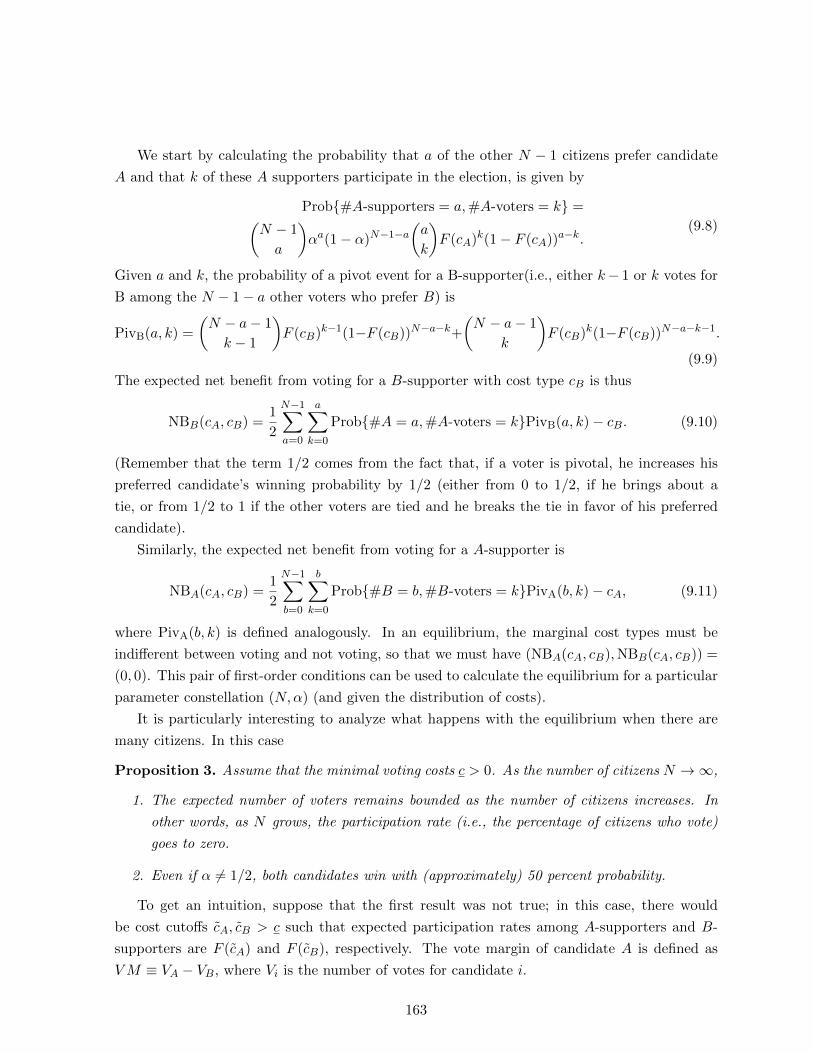
We start by calculating the probability that a of the other N − 1 citizens prefer candidate

A and that k of these A supporters participate in the election, is given by

Prob{#A-supporters = a,#A-voters = k} =(N − 1

a

)αa(1− α)N−1−a

(a

k

)F (cA)k(1− F (cA))a−k.

(9.8)

Given a and k, the probability of a pivot event for a B-supporter(i.e., either k− 1 or k votes for

B among the N − 1− a other voters who prefer B) is

PivB(a, k) =

(N − a− 1

k − 1

)F (cB)k−1(1−F (cB))N−a−k+

(N − a− 1

k

)F (cB)k(1−F (cB))N−a−k−1.

(9.9)

The expected net benefit from voting for a B-supporter with cost type cB is thus

NBB(cA, cB) =1

2

N−1∑a=0

a∑k=0

Prob{#A = a,#A-voters = k}PivB(a, k)− cB. (9.10)

(Remember that the term 1/2 comes from the fact that, if a voter is pivotal, he increases his

preferred candidate’s winning probability by 1/2 (either from 0 to 1/2, if he brings about a

tie, or from 1/2 to 1 if the other voters are tied and he breaks the tie in favor of his preferred

candidate).

Similarly, the expected net benefit from voting for a A-supporter is

NBA(cA, cB) =1

2

N−1∑b=0

b∑k=0

Prob{#B = b,#B-voters = k}PivA(b, k)− cA, (9.11)

where PivA(b, k) is defined analogously. In an equilibrium, the marginal cost types must be

indifferent between voting and not voting, so that we must have (NBA(cA, cB),NBB(cA, cB)) =

(0, 0). This pair of first-order conditions can be used to calculate the equilibrium for a particular

parameter constellation (N,α) (and given the distribution of costs).

It is particularly interesting to analyze what happens with the equilibrium when there are

many citizens. In this case

Proposition 3. Assume that the minimal voting costs c > 0. As the number of citizens N →∞,

1. The expected number of voters remains bounded as the number of citizens increases. In

other words, as N grows, the participation rate (i.e., the percentage of citizens who vote)

goes to zero.

2. Even if α 6= 1/2, both candidates win with (approximately) 50 percent probability.

To get an intuition, suppose that the first result was not true; in this case, there would

be cost cutoffs cA, cB > c such that expected participation rates among A-supporters and B-

supporters are F (cA) and F (cB), respectively. The vote margin of candidate A is defined as

VM ≡ VA − VB, where Vi is the number of votes for candidate i.

163

For N large, the expected number of votes for A, VA is approximately normally distributed,

with expected value E(VA) = αF (cA)N and variance σ2V A = αF (cA) [1− αF (cA)]N .2 Similarly,

the expected number of votes for B, VB is approximately normally distributed, with expected

value E(VB) = (1 − α)F (cB)N and variance σ2V B = αF (cB) [1− αF (cB)]N . The random

variable VM is approximately normally distributed, with expected value

E(VM) = E(VA)− E(VB) = [αF (cA)− (1− α)F (cB)]N (9.12)

and variance

σ2VM = σ2V A + σ2V B = {αF (cA) [1− αF (cA)] + αF (cB) [1− αF (cB)]N}N. (9.13)

Consider the event that VM ∈ [−1, 1]. This is an upper bound for the probability of a pivot

event (because an A-supporter is pivotal if VM ∈ {−1, 0}, and a B-supporter is pivotal if

VM ∈ {0, 1}).Let Φ(·) denote the cumulative distribution function of the standard normal distribution

(i.e., the one with expected value µ = 0 and standard deviation σ = 1. Remember that the

probability that a random variable that is normally distributed with expected value µ and

standard deviation σ takes a value of less than x is Φ(x−µ

σ

). Given that VM is approximately

normally distributed with expectation and variance given above, we have that

Prob(VM ∈ [−1, 1]) = Φ

(1− [αF (cA)− (1− α)F (cB)]N√

(αF (cA) [1− αF (cA)] + αF (cB) [1− αF (cB)])N

)−

Φ

(−1− [αF (cA)− (1− α)F (cB)]N√

(αF (cA) [1− αF (cA)] + αF (cB) [1− αF (cB)])N

) (9.14)

This expression goes to zero as N goes to infinity. To see this, consider three possible cases. First,

if the expected number of votes for A and B are equal (i.e., if αF (cA)− (1−α)F (cB) = 0), then

both arguments of Φ go to zero as N →∞, and obviously Φ(0)−Φ(0) = 0. Alternatively, if A’s

expected vote number is larger than B’s expected vote number (i.e., if αF (cA)− (1−α)F (cB) >

0), then both arguments of Φ go to infinity as N →∞, so that Φ(∞)−Φ(∞) = 1− 1 = 0. The

third case, namely that A’s expected vote number is lower than B’s expected vote number (i.e.,

if αF (cA)− (1− α)F (cB) < 0), is analogous.

In summary, if the participation rate was positive as N grows, then the pivot probability for

each citizen would go to zero. However, if that is the case, then it does not make sense to spend

the cost of voting. This proves that the expected number of voters must be finite as N →∞.

As a consequence, both voter preference types’ cost cutoff must converge to c as N → ∞,

i.e., only very few low cost citizens vote. Random variables such as VA and VB that are the

result of many trials that each have a very low success probability are best modeled as Poisson

2These are standard formulas for binary random variables given that the success probability per trial is αF (cA).

164

distributed, where the parameters of the two Poisson distributions are the expected number of

voters, E[VA] and E[VB], respectively. This implies that E[VA] = E[VB] in the limit, because the

pivot probabilities for A and B would differ otherwise. Therefore, VA and VB are independent

and identically distributed random variables. Hence, P ({VA > VB}) = P ({VB > VA}), which

implies that each candidate has the same probability of winning the election. Thus, in the

limit, voluntary voting results in the correct outcome (from a social point of view) only with

probability 1/2.

9.4.2 Welfare analysis

What do the positive results imply for welfare? Should a social planner marginally encourage

or discourage participation in elections?

To decide this question, we have to analyze the direction of the voting externality. Suppose

we induce one more citizen to vote, say, by a very small subsidy (making voting a little less

costly). Note that this citizen was (almost) indifferent between voting and not voting, meaning

that the positive aspects of voting (i.e., the chance of influencing the outcome of the election

in favor of his preferred candidate) just balance the negative aspects (i.e., the cost of voting).

Therefore, when considering the welfare effect of inducing this citizen to vote, we can neglect

this citizen’s direct expected payoff, which is zero.

If, among the other voter, one of the candidates is clearly ahead, then the election outcome

does not change, and there is also no external effect on their welfare. In contrast, if the other

voters are (almost) tied, the additional voter may change the outcome. The externality on the

other people who vote is (almost) zero because there is (essentially) the same number of A-voters

and B-voters.3

If the additional voter is a majority type, the majority of non-voters benefits; if, instead,

the additional voter is a minority type, the majority of non-voters suffers. However, it is more

likely that a marginal voter attracted to the polls is a majority type than a minority type. This

follows from two observations: First, by definition, there are more citizens who are majority

types. Second, because in equilibrium minority types vote at a higher rate than majority types

(otherwise, the majority-preferred candidate would almost surely win), among non-voters, the

majority-types are overrepresented. Thus, since the marginal additional voter is more likely to

be a majority types, the overall expected net externality is positive, and so, from a social point

of view, should be encouraged to vote.

We will now make this point in a more formal way in the framework analyzed above. The

citizens’ average outcome payoff in large elections under voluntary voting is 12α+ 1

2(1−α) = 12 ,

3In those cases in which the vote of the additional voter is pivotal for changing the outcome distribution, there

is either a tie between the other A and B voters, or the candidate preferred by the additional voter is one vote

behind among the other voters. In the latter case, there is a small negative externality on the other voters, but

this effect is very small in large electorates.

165

because, even if α 6= 1/2, both candidates win with (approximately) 50 percent probability.

Moreover, since hardly anybody votes, the voting cost per capita is negligible, so the average

outcome payoff is also the average net payoff under voluntary voting.

What would happen if, instead, we forced everybody to vote (or, alternatively, subsidized

voting by at least c so that each citizen has a non-positive cost of voting, and therefore all

will find it in their own interest to vote). If everybody votes, the majority-preferred candidate

is guaranteed to win, and the outcome payoff per capita (in a large electorate) is therefore

max(α, 1−α) ≥ 1/2. However, the perfect track record regarding the selection of the majority-

preferred candidate comes at the cost of everybody having to vote, and the per-capita cost

for this is E(c) =∫ cc cf(c)dc. Thus, the total per capita payoff under compulsory voting is

max(α, 1−α)−E(c). This may be larger or smaller than the per-capita payoff under voluntary

voting, depending on whether |α− 12 | R E(c).

The optimal subsidy in a large society is to set the subsidy equal to the minimum voting

costs (or maybe just a bit more). This guarantees participation of a small percentage of the

electorate who have zero net voting costs. Even a small (but strictly positive) percentage of

the electorate consists of a sufficiently large number of voters to be representative, so that the

majority-preferred candidate is almost sure to win, and per-capita outcome utility is approx-

imately max(α, 1 − α), just as under compulsory voting. However, in contrast to compulsory

voting, this perfect selection is achieved at (close to) zero per-capita cost, so that max(α, 1−α)

is also total per-capita utility in this minimal-cost subsidy regime.

9.5 Costly voting in finite electorates

Costly voting models predict very low turnout if voting is motivated by the chance to influence

the outcome of the election. This is sometimes called the “paradox of not voting”. Of course, all

real-world electorates are finite, so the prediction that participation rates go to zero if the size of

the electorate goes to infinity may not be relevant if real-life electorates are still relatively small.

To get a better feeling about the probability of being pivotal for the outcome in a large election,

consider an electorate that is, in expectation, perfectly split 50:50 between A-supporters and

B-supporters. If N other citizens go to vote, the probability that they are split exactly half-half

between the candidates is

Pivot(N) =

(N

N/2

)1

2

N

(9.15)

For N = 10, this probability is approximately 24.6 percent, so the probability of affecting the

outcome in small split electorates is quite large. Since the binomial coefficient is difficult to

calculate exactly for large N , it is useful to use Sterling’s approximation formula that says that

N ! ≈√

2πN

(N

e

)N. (9.16)

166

Using this in (9.15) gives

Pivot(N) =N !

(N/2)!(N/2)!

1

2

N

≈√

2πN(Ne

)N(√πN

(N/2e

)N/2)2

1

2

N

=

√2

πN(9.17)

For N = 1000, this approximation is already very close to the exact value of about 2.52 percent.

Every time the size of the electorate grows by a factor of 100, the pivot probability decreases

to a tenth of its previous value. So in an election with 100, 000 voters, the probability of a tie

is about 0.25 percent, and if there are 10, 000, 000 voters, that probability is 0.025 percent, or

about 1 in 4000.

How does this compare to the cost of voting? The best-case scenario is probably that voting

takes 15 minutes, including the way to the polling station, minimal waiting time there, plus the

time for filling out the ballot; clearly, it may also take substantially longer. So, the value that

voters must attach to affecting the outcome of the election in order to justify the act of voting is

at least the equivalent of 4000× 14 hours = 1000 hours of time for an election in which 10 million

people participate (say, a gubernatorial election in a large state), and at least the equivalent of

100 hours for an election with 100,000 participants.

1000 hours is about the working time in half a year. How many people would be willing to

give the income of half a year if that would allow them to determine the winner of a gubernatorial

election? Some would, probably, but it seems likely that a lot of the people who vote attach a

lower value to the election outcome, especially considering that a lot of people spend considerably

more time for voting than the 15 minutes that were our best-case scenario.

There is another reason why our numerical examples likely overstate the instrumental benefit

of voting: In the examples above, we assume that the expected vote share for candidate A is

exactly equal to 0.5. How would the results change if instead the expected proportion of A-voters

is, say, 0.49 or 0.499? Intuitively, this would still qualify as a very tight election, but it is not

any more exactly equal to 1/2.

Denoting A’s expected vote share by α,4 the pivot probability is

Pivot(N) =N !

(N/2)!(N/2)!αN/2(1− α)N/2 ≈

√2πN

(Ne

)N(√πN

(N/2e

)N/2)2αN/2(1− α)N/2

=

√2

πN[4α(1− α)]N/2

(9.18)

The value of the extra factor in (9.18) (relative to (9.17)), [4α(1− α)]N/2 depends a lot on N . For

example, suppose that α = 0.499; for N = 1000, the extra factor is approximately 0.998 so that

the difference between the case of α = 0.5 and α = 0.499 is trivial. However, for N = 100000,

4This is a slight abuse of notation. In the previous sections, α was the expected percentage of A-supporters

among citizens, and that might be different from that percentage among voters.

167

the factor is about 0.819 so that the pivot probability is reduced by about 20 percent relative to

the baseline case, and for N = 10, 000, 000, the factor is approximately equal to 2 × 10−9. So,

in the latter case, the chance of being pivotal is reduced from 0.025 percent in case of α = 0.5

(unlikely, but not impossible; 1 case out of 4000) to extremely unlikely 5 ∗ 10−13.

To justify voting in this case would require an implausibly high value attached to the outcome

of the election, or an extremely small cost of voting. So how do we interpret the fact that people

seem to participate in elections at considerably higher rates than suggested by the analysis of

the costly voting model. There are three possible interpretations.

First, people might overestimate the probability that their vote could make a difference for

the election outcome. They hear from many sources that “every vote matters”, and the possi-

bility to learn that this is rarely literally true is extremely limited: For example, suppose that

voters in large swing states in tight Presidential elections mistakenly believe that the proba-

bility of their own vote making a difference is 0.5 percent, much higher than in reality; this is

high enough to justify to exert some effort for participating, considering the importance of a

presidential election. However, given that an individual observes at most maybe 12 close Presi-

dential elections during his lifetime, the absence of a tie actually occurring is not really damming

evidence. The individual cannot easily infer that his probability belief is likely incorrect.

Second, people may receive an intrinsic benefit from voting that outweighs the direct mon-

etary and time costs; they may feel a sense of “civic duty” to vote. There are lots of low cost

“public good provision” problems in which explicit government intervention to deal with the

problem would be very expensive, while it is much more effective to teach the socially desired

behavior in school in order to permanently affect the preferences of the individuals. For exam-

ple, think of why you (probably) do not throw your small trash on the floor or on the street,

but rather go to a wastebasket to discard it. This action is sometimes costly in the sense that

it takes some time to find a wastebasket. True, there are fines for littering, but the chance of

being caught is sometimes minimal. What explains the “paradox of not throwing trash on the

street”? Probably, education in schools from a very early age that it is not ok to litter has

permanently affected the payoff structure of most individuals (admit it, you would probably feel

bad if you litter, even if nobody sees it). This education approach is socially beneficial. We are

better off as a society if most people don’t litter, and enforcing this any other way (say, through

explicit fines and enforcement) would be very expensive and not very effective. What the costly

voting model shows is that, in a society populated by people who only look for their own direct

advantage, too few people (rather than too many people) would be voting. Therefore, it is a

good idea to instill this civic duty feeling through education in schools, emphasizing the value

of voting for a democratic society.

Third (and related to the second point), people may choose to vote because they have a “cost

of not voting, ” for example, moral pressure from family and friends. Effectively, this external

moral pressure works in the same way as an explicit subsidy of the cost of voting, in the sense

168

that it increases participation over the equilibrium level.

169

Index

allocation mechanisms, 44

competitions, 47

lotteries, 47

queuing, 45

selling, 45

applications

emissions reduction, 27

black market, 42

compensating variation, 10

numerical example, 12

consumer surplus, 38

contract curve, 19

core, 19

cost-benefit analysis, 8

demand function, 37

compensated (Hicksian), 9

uncompensated (Marshallian), 9

dual household problem, 9

duality, 9

Edgeworth box, 16

disequilibrium, 20

equilibrium, 20

initial endowment, 16

efficiency

exchange, 22

optimal product mix, 27

product mix, 26

with production, 24

emissions reduction, 27

equivalent variation, 10

numerical example, 12

expenditure minimization problem, 9

externality, 73

First theorem of welfare economics, 22

Hicksian demand function, 9

household

utility maximization problem, 9

indirect utility function, 9

isoquant, 23

marginal rate of substitution, 22

marginal rate of technical substitution, 23

marginal rate of transformation, 26

marginal willingness to pay, 37

Marshallian demand, 9

Nash equilibrium, 59

non-price allocation methods, 44

normative economics, 15

Pareto better, 16, 17

Pareto comparison, 17

Pareto efficiency, 17

with production, 23

Pareto improvement, 16, 17

Pareto optima

set of, 19

Pareto optimality, 17

Pigou tax, 30

pollution reduction

170

command-and-control, 30

efficiency, 29

Pigou tax, 30

pollution rights, 31

tradeable permits, 31

positive economics, 15

preference ranking, 5

completeness, 6

continuity, 7

monotonicity, 7

reflexivity, 6

transitivity, 6

primal (household) problem, 9

production possibility frontier, 24

ranking

completeness, 6

transitivity, 6

rationing

efficient, 42

random, 42

second theorem of welfare economics, 32

supply function, 38

technical efficiency, 24

transformation curve, 24

utilitarianism, 4

utility function, 5

ordinal vs. cardinal interpretation, 8

preference ranking, 5

existence, 7

utility maximization problem, 9

value function, 9

welfare analysis

agricultural subsidies, 43

excise tax, 39

price ceiling, 41

subsidy, 33, 41

welfare loss, 40

171