
PSU-IRL-SCI-405 Classification Numbers 1.5.3, 3.1.3, and 3.2 · 2013-08-31 · psu-irl-sci-405...
63
PSU-IRL-SCI-405 Classification Numbers 1.5.3, 3.1.3, and 3.2.2 THE PENNSYLVANIA STATE UNIVERSITY IONOSPHERIC RESEARCH Scientific Report 405 AN EXPERIMENTAL INVESTIGATION OF THE POWER SPECTRUM OF PHASE MODULATION INDUCED ON A SATELLITE RADIO SIGNAL BY THE IONOSPHERE by David T. Moser December 12, 1972 The research reported in this document has been sponsored by the National Science Foundation under Grant GA-12228 and by the National Aeronautics and Space Administration under Grant NGR 39-009-002. IONOSPHERE RESEARCH LABORATORY C tl r F.n ::; PI Z-t os C H kiD' - i Fq) Ntj tj t: OjH 0 rj t jl! tx h t JtM Ul tC L co tri 0 - t-H C rr Co -JH iw 0 -j Z C) - j an W S -'. 00 Reproduced by NATIONAL TECHNICAL INFORMATION SERVICE US Department of Commerce Springfield, VA. 22151 University Park, Pennsylvania ~~~~~ I I '1 :f "! [;? https://ntrs.nasa.gov/search.jsp?R=19730011451 2020-04-08T11:49:30+00:00Z
Transcript of PSU-IRL-SCI-405 Classification Numbers 1.5.3, 3.1.3, and 3.2 · 2013-08-31 · psu-irl-sci-405...
PSU-IRL-SCI-405Classification Numbers 1.5.3, 3.1.3, and 3.2.2
THE PENNSYLVANIASTATE UNIVERSITY
IONOSPHERIC RESEARCH
Scientific Report 405
AN EXPERIMENTAL INVESTIGATION OF THEPOWER SPECTRUM OF PHASE MODULATION
INDUCED ON A SATELLITE RADIO SIGNALBY THE IONOSPHERE
byDavid T. Moser
December 12, 1972
The research reported in this document has been sponsored bythe National Science Foundation under Grant GA-12228 andby the National Aeronautics and Space Administration underGrant NGR 39-009-002.
IONOSPHERE RESEARCH LABORATORY
C tl r F.n
::; PI Z-t osC H kiD'
- i Fq)
Ntj tj t:
OjH 0
rj t jl! txh t JtMUl tC L
co tri 0- t-H C
rr Co-JH
iw
0
-j
Z
C) - j
an W S
-'.
00
Reproduced by
NATIONAL TECHNICALINFORMATION SERVICE
US Department of CommerceSpringfield, VA. 22151
University Park, Pennsylvania
~~~~~ I
I
'1 :f "! [;?
https://ntrs.nasa.gov/search.jsp?R=19730011451 2020-04-08T11:49:30+00:00Z

Securitv Ca .ssi `ication
DOCUMENT CONTROL DATA - R & DSec'lrrity cl.asssific' atio, of title, body ot¢,i abf r t eard ildexin,: ,.1nnolaticn nius I be entered when the overall report is ch;,isified)
I. ORIGINA TING AC TIV I TY (Corporate author) 2a. REPORT SECURITY CLASSIFICATION
Ionosphere Research Laboratory 2b. GROUPAiar
3. REPORT TITLE
An Experimental Investigation of the Power Spectrum of Phase Modulation Inducedon a Satellite Radio Signal by the Ionosphere
4. DESCRIPTIVE NOTES (Type of report and.inclusive dates)
Scientific ReportS. AUTHOR(S) (First name, middle initial, last name)
David T. Moser
6. REPORT DATE 7a. TOTAL NO. OF PAGES 7b. NO. OF REFS
December 12, 1972 6480. CONTRACT OR GRANT NO. J9. ORIGINATOR'S REPORT NUMBER(S)
NASA NGR 39-009-002NSF GA- 12228 PSU-IRL-S CI-405
b. PROJECT NO.
c. - 9b. OTHER REPORT NO(S) (Any other numbers that may be assignedthis report)
d.
10. DISTRIBUTION STATEMENT
Sponsoring Agencies
11. SUPPLEMENTARY NOTES 12. SPONSORING MILITARY ACTIVITY
National Aeronautics and SpaceAdministration
National Science Foundation13. ABSTRACT
The object of this study was to investigate the power spectrum of phasemodulation imposed upon satellite radio signals by the inhomogeneous F-regionof the ionosphere (100 - 500 km). Tapes of the S-66 Beacon B Satellite recordedduring the period 1964 - 1966 were processed to yield or record the frequencyof modulation induced on the signals by ionospheric dispersion. This-modulation is produced from the sweeping across the receiving station (State College,Pennsylvania) as the satellite transits of the two-dimensional spatial phasepattern are produced on the ground. From this a power spectrum of structuresizes comprising the diffracting mechanism was determined using digitaltechniques. Fresnel oscillations were observed and analyzed along with somecomments on the statistical stationarity of the shape of the power spectrumobserved.
DD 1N0 V61473 (PAGE 1)/N 0101-807-681S/N 0101-807-6811
' -2 NONE-Security Classification
A-31408
- .. .

PSU-IRL-SCI-405Classification.Numbers 1.5.3, 3. 1.3, and 3.2. 2
Scientific Report 405
An Experimental Investigation of the Power Spectrumof Phase Modulation Induced on a.Satellite
Radio Signal by: the Ionosphere
by
David T. Moser
December 12, 1972
The research reported in this document has been sponsored by theNational Science Foundation under Grant GA-12228 and by theNational Aeronautics and Space Administration under GrantNGR. 39-009-002.
Submitted by:
Approved by:
W. JS RoJs, Head, Department ofElectrtc,2f1 EngineeringProjecfSupervisor
JD Je Gibboe te Professor Emeritus,Department of ysics
A. J. Ferraro, Acting DirectorIonosphere Research Laboratory
Ionosphere Research Laboratory
The Pennsylvania State University
University Park, Pennsylvania 16802
f
C'. D-.
- ii -
ACKNOWLEDGMENTS
I wish to express my appreciation and indebtedness
to Dr. W. J. Ross for his invaluable guidance and assistance
throughout the course of the research reported here. I also
wish to thank Dr. J. J. Gibbons and the staff of the hybrid
computer facility at P.S.U. for their helpful assistance.
This work was supported by NASA Grant NGR 39-009-002
and also in part by NSF Grant GA 12228.

- iii -
TABLE OF CONTENTS
Page
ACKNOWLEDGMENTS. . . . . . . . . . . . . .
LIST OF TABLES . . . . . . . . . . .
LIST OF FIGURES. . . . . . . . . . .
I INTRODUCTION ...... .. . . .
1.1 Previous Related Studies. . . . .1.2 Statement of the Problem. . . .
ii
· .
e ·
·. . ·. .·
II THEORY OF DIFFRACTION DUE TO AN INOHMOGENEOUSIONOSPHERE. . . . . . . . . . . . . . .
Diffraction Theory . . . . . . . . . . . .Fourier Analysis of a Weakly Refracting Screen.Strongly Refracting Medium. . . . . . . . .Characteristics of the Inohmogeneous F-Region .Diffraction by an Inhomogeneous Ionosphere.. .
SIGNAL HANDLING AND DATA REDUCTION EQUIPMENTAND TECHNIQUES . . . . . . . . . . . . . . .
Source and Initial Signal Handling.Analog Processing . . . . . . . . . . . . .Data Analysis . . . . . . . . . . . . . . . . .
IV EXPERIMENTAL RESULTS. . .. . . . . . . . .
Experimental Details. ..Spectral Density of the Frequency Modulation.Discussion of the Results . . . . . . .
SUMMARY . . . . . . . . . . . . . . . . . . .
Conclusion. . . . . . . . . . . . . . .Suggestions for Future Work . . . . . . . . .
BIBLIOGRAPHY . . . . . . . . . .
APPENDIX A . . . . . . . . .
APPENDIX B . . . . . . . . . . . . . . . . . . . ..
iv
v
1
13
4
48
111416
21
212429
35
353743
47
4748
50
52
56
2.12.22.32.42.5
III
3.13.23.3
4.14.24.3
V
5.15.2
0
0
. .··
· · i ··
e · .·
· · · · I ·' · · ·

- iv -
LIST OF TABLES
Table
I Orbital Parameters and Experimental Results. .
Page
36

v -
LIST OF FIGURES
Figure Page
1 Flat earth geometry of the satellite, iono-sphere, receiver system. . . . . . . . . . . . . 15
2 Block diagram of the receiving equipment . . . . 22
3 Block diagram of filtering and discriminatorcircuitry. . . . . . . . . . . . . . . . . . . . 25
4 Frequency modulation caused by the apparentdoppler dispersion for (a) flat earth, (b)curved earth geometry, . . . . . . . . . . . . . 27
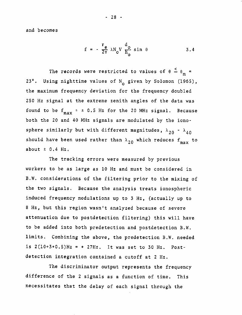
5 Sample record of discriminator output f(t) . . . 30
6 Unsmoothed power spectrum for orbit 6173 . . . . 38
7 Smoothed power spectrum for orbit 6173 . . . . . 38
8 Smoothed power spectrum for orbit 10566. . 39
9 Smoothed power spectrum for orbit 8550 .. . . 39
10 Smoothed power spectrum for orbit 9356 . . . . . 40
11 Smoothed power spectrum for orbit 9397 . . . . .40
12 Flow diagram of data analysis program. . . . . 54
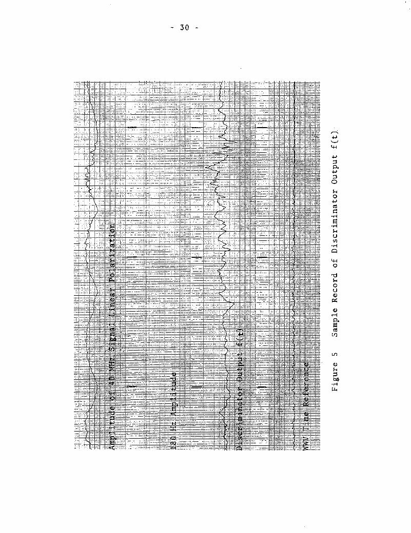
13 Flow diagram continued . . .. . . . . . . 55
14 Sample of a record of the processed data whichis stored before processing on magnetic tape . . 56

CHAPTER I
INTRODUCTION
1.1 Previous Related Studies
The ionosphere is the region of the upper atmosphere
comprised of neutral and ionized gases and free electrons.
The presence of free ions and electrons is caused mainly by
photoionization during direct sunlight conditions, and is
maintained during nighttime conditions by the finite recom-
bination rates of the ionized-particles. Although there are
not any definite boundaries given to this region, it is
generally considered to start at an altitude of 50 km and
continue upward to the interface between the atmosphere and
the solar wind.
Active investigation of this region began half a
century ago when it was observed (Appleton and Barnett 1925)
that radio waves from ground based senders were reflected
from an altitude of 100 to 200 km. Using this reflection
technique, researchers were able to generate fairly detailed
descriptions of the ionosphere. They also found that the
ionized medium was not uniform or static, but at times con-
tained random fluctuations in electron density which caused
amplitude fluctuations or scintillations of the returned
echoes. Further investigations of this effect produced some
information on the size and motion of these inhomogeneous
structures.
This method contained two fundamental difficulties:
!

(1) it was limited to analysis of the region below the
height of maximum ionization since no reflections could be
obtained from greater heights, (2) the mathematical descrip-
tion of this process near the reflection point was complex
and obscured the interpretation of the experimental data.
A new experimental technique was introduced by Hewish (1951)
which eliminated the first problem and reduced the complexity
of the second. He introduced the idea of using a radio star
with its higher frequencies as the source in a transmission
experiment. Further improvement has occurred in the last
ten years with the introduction of satellite radio sources.
These have the advantage of providing very coherent and
stable signals with the ability to scan large sections of
the ionosphere very quickly during the transit of the satel-
lite across the field of view of a receiving station.
To date most transmission experiments have dealt
with the amplitude variations of the radio signal. Ampli-
tude studies by Spencer (1955) showed the irregularities to
be elongated along the magnetic field lines, and studies by
Jones (1960) produced a range of apparent sizes of these
structures, Further studies (Jespersen et alo, 1964; Dyson,
1969; Kelleher et al., 1970; Rufenach et al., 1972) have
produced information on the statistical nature of their
location, size, and shape.
The experimental use of phase fluctuations rather
than amplitude scintillation, has not received much
attention except for a study by Porcello and Hughes (1968)

- 3 -
due probably to its much greater experimental complexity.
As will be shown later, however, the use of phase infor-
mation has the advantage of allowing the observation of
larger structure sizes than by amplitude studies for a given
source frequency and allowing a more direct interpretation
of the results in terms of the ionospheric characteristics.
1.2 Statement of the Problem
The object of this study is to investigate the power
spectrum of phase modulation imposed upon satellite radio
signals by the inhomogeneous F-region of the ionosphere
(100-500 km). Records containing the signals will be pro-
cessed to yield temporal variations resulting predominately
from the sweep across a receiving station as the satellite
transits, of the two-dimensional spatial phase pattern
produced on the ground. This will then be linked to the
power spectrum of structure sizes comprising the diffracting
medium. It is hoped that these results may provide useful
information on the nature of the diffracting medium and on
possible production mechanisms for its inhomogeneous nature.

CHAPTER II
THEORY OF DIFFRACTION DUE TO AN INHOMOGENEOUS IONOSPHERE
2.1 Diffraction Theory
It is necessary to develop a physical model and the
associated mathematical description of the transmission
experiment being conducted. The most general model is that
of a moving point source at a finite distance from the
diffracting medium of finite thickness. The motion of the
source will cause the geometry of the problem to change by
changing the angle of incidence upon the medium and the
distances between source and diffracting medium and observer.
The simplified model to be used is of a uniform, unit ampli-
tude plane wave normally incident upon a thin diffracting
medium. Later the restriction to use of a plane wave
(source at infinite distance) will be lifted. Use will be
made of diffraction theory (outlined by Ratcliffe 1956) to
describe the physical model used.
The diffracting medium modifies both the amplitude
A and phase ~ of the plane wave, so that as it leaves the
medium it possesses a complex amplitude f (x,y) across the
plane parallel to the medium (complex quantities are indi-
cated by a bar) given by:
f(x,y) = A(x,y) exp[iq(x,y)] 2.1
The wave field immediately below the plane of the medium,
//

- 5 -
and hence at all points in this half-space, can be repre-
sented by an angular spectrum of plane waves A (01,62)
incident upon the diffracting medium at the angles 81,82
(01 is the complement of the angle between the propagation
vector k and the x axis, similarly for 82 and the y axis).
What this involves is taking the vector sum of the angular
components shifted in phase by an appropriate amount, with
x=y=O taken as the reference point for zero phase shift.
Letting C = cos ej and S. sin ej for j = 1,2, A(61,8
2)
becomes
A(801, 2 ) = F(S1,S2)
The complex amplitude in terms of its angular spectrum is
(lower case dimensions and coordinates x,y,z are normalized
in terms of wave length X, upper case letters represent
unnormalized distances)
- a1 1-(xpy) ·1 -l' F(S1,S 2 ) exp[2ni(Slx + S2 Y)]dsl ds2
2.2
As the wave front leaves the medium the individual elements
of F(S1,S2) are shifted in phase by an amount 2nC3 z. As
used here, the sines of 01 and 82 along with C3 form the
direction cosines of k(81,8
2). C3 is related to 81 and 82
by

- 6 -
C3 = [- cos( - el + 2- 62) cosQ - e 2
or
C3 = [cos(e1 + 62) cos (01 - e2)]1
For a given distance from the screen, equation 2.2 becomes
f(x,y,z) = 1 f F(S1'S2) exp[2fi[Slx + S2y + C3 z)]dsl ds
2
2.3
When S > 1, (1 - C2 ) > 1 yields imaginary values for C.
Letting C3 = iy for real y, the term exp(27iC3z) in equation
2.3 becomes exp(- 2ryz). Waves with S > 1 are therefore
greatly attenuated as they leave the screen and so carry no
power away from the screen. They are commonly referred to
as evanescent waves. For the consideration of wave fields
at a distance of many wavelengths below the medium, the
limits of integration in equations 2.2 and 2.3 can be
extended to + ~ to yield
f(x,y,z) = : X F(S1 ,S2 ) exp[27i(Slx + S2y + C3 z)]ds1 ds2
Previously phase was measured w.r.t. the carrier at
the diffracting medium. In evaluating the spectrum at a
distance z from the screen, only phase measured w.r.t. the
carrier at the point of observation will be used. This
change is accomplished by subtracting the phase factor 27iz

- 7 -
from the 2riC3z term above to yield
f (x,y,z) = f c F(S1,S 2) exp[2wi(Slx+S2 y+(C3-1)z)]dsl ds2
2.4
Comparing equation 2.4 with 2.2, f(x,y,z) is composed of a
complex angular spectrum
G(SlS2 ,z) = F(Sl,S2) exp[27ri(C3 - 1)z] 2.5
which can be thought of as the function F(S1,S 2) with its
components shifted in phase to account for propagation in
different directions to a distance z from the screen. As
will be shown later, it is f(x,y,z) which is actually mea-
sured and the angular spectrum is used as a means of deter-
mining the nature of the diffracting medium from the measured
pattern f(x,y,z). Equation 2°4 is the expression for a
Fourier transform pair, with z as a parameter, and can be
represented as:
f(x,y,z) ++ G(S1,S2,z) 2.6
If the case of a diffracting medium with no absorp-
tion (which is a good approximation for the F-region at the
frequencies used) is considered, f(x,y,0) will contain only
phase variations. This is equivalent to setting A(x,y) = 1
in equation 2.1. An attempt will be made to obtain pre-
dictions about the properties of the diffraction pattern by
J

- 8 -
considering a simple diffracting medium with a cosinusoidal
variation of phase shift with position. The generalization
of this model to more complex medium distributions will be
then considered. The inversion of the results of this
analysis will provide a basis for interpreting experimentally
obtained data.
2.2 Fourier Analysis of a Weakly Refracting Screen
In the interest of simplicity only variations in the
x direction will be considered. Let f(x,O) consist of a
cosinusoidal phase variation imposed on a unit amplitude
carrier given by
f(x,O) = exp(i4o cos 2w) 2.7
where d is the periodicity of the modulation and therefore
of the screen. If %o << 1, then f(x,o) = 1+ i o cos 21T
which can be shown to have the following angular spectrum
(the values of S in the parentheses indicating the angle of
the component).
F(S) = 1 (S = 0) + -- (S ) (S =
The first term represents the carrier and the other two
terms are phase quadrature terms. Letting the integral in
equation 2.4 (without the y dependence) become a sum,
f(x,z) becomes:
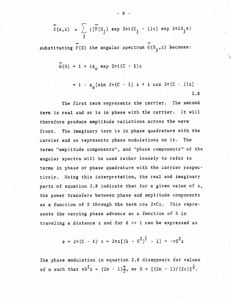
- 9-
f(x,z) = j {[F(Sj) exp 2wi(Cj - 1)z] exp 2riS.x}
substituting F(S) the angular spectrum G(Sj,z) becomes:
G(S) = 1 + i4o exp 27i(C - l)z
= 1 - .e[sin 2w(C - 1) z + i cos 2(rrC - l)z]
2.8
The first term represents the carrier. The second
term is real and so is in phase with the carrier. It will
therefore produce amplitude variations across the wave
front. The imaginary term is in phase quadrature with the
carrier and so represents phase modulations on it. The
terms "amplitude components", and "phase components" of the
angular spectra will be used rather loosely to refer to
terms in phase or phase quadrature with the carrier respec-
tively. Using this interpretation, the real and imaginary
parts of equation 2.8 indicate that for a given value of z,
the power transfers between phase and amplitude components
as a function of S through the term cos 27rCz. This repre-
sents the varying phase advance as a function of S in
traveling a distance z and for d i> 1 can be expressed as
= 2·(C - 1) -z= 2=z[(1 - S2)~'- 1]2 = ~S2z
The phase modulation in equation 2.8 disappears for values
2 or S = [(2n- 1)/(2z)]2of n such that wS z = (2n - 1)T, or S = [(2n.- 1)/(2z)]2 .

- 10 -
What this means is that for S << 1/(2z), only phase effects
will be present, but amplitude components will dominate the
angular spectrum as S approaches the case for n = 1. There-
fore for screen periodicities d near
1 2z ld = = [ n -1 ] n = 1,2, . 2.9
The phase modulations produced at the diffracting medium
will appear as amplitude variations at a distance z, which
will tend to produce nulls in any phase spectrum for the
conditions of equation 2.9. The nulls will not be very
sharp due to the motion of the satellite causing variations
in the effective height of the diffracting layer with
latitude. There is also the change in Zl, z2 , and ho with
zenith angle. Both these effects tend to change the values
of d for which the nulls occur and therefore produce shallow
nulls. Only the first null will have much chance of being
observable due to its large separation from the second null.
The case for S << 1/(2z) will be of primary concern in any
study of phase fluctuations because for a thin screen under
this restriction the pattern on the ground is a simple pro-
jection of the screen.
Until now it has been assumed that the source is at
an infinite distance from the diffracting screen. The
actual case is a source at a finite distance. As was shown
by Briggs and Parkin (1963) the change is accomplished by
replacing z by Zl Z2/(z
1+ z
2), where z1 = hi, z
2= h
o- h
i

- 11
shown in figure 1. This yields the following expression
which replaces equation 2.8:
z2
G(S,z) = 1 - 0o sin[2r(C - l)zi
o-i
2.10z2
+i O cos [2r(C - l)z1 io]
For z2, h
o>> Zl, equation 2.10 approaches 2.8 since
z2/(z1+ z2 ) + 1, but as zl increases w.r.t. z2 the ratio
z /h° decreases until for z1 = z2, z2 /h° = 1/2, This ex-
treme case won't occur for the restricted zenith angles
encountered in our experiment but ratios on the order of 70
could occur. The effect this has on equation 2.9 is to
lower the sizes of d for which nulls occur by the factor
z2 /ho to produce
221 z2d = [Zn - 1 (-) ] 2.11
2.3 Strongly Refracting Medium
Previously only weak scattering was examined. It
will be shown that there is also the need for considering
cases other than «o << 1. The consequence of this
inequality not holding is seen most clearly by looking at
equation 2.1. For amplitude effects (4(x,y) = 0) there is
a linear relationship between f(x,y) and A(x,y) independent
of the size of the amplitude fluctuations imposed by the
medium. This will allow A to be broken into its Fourier
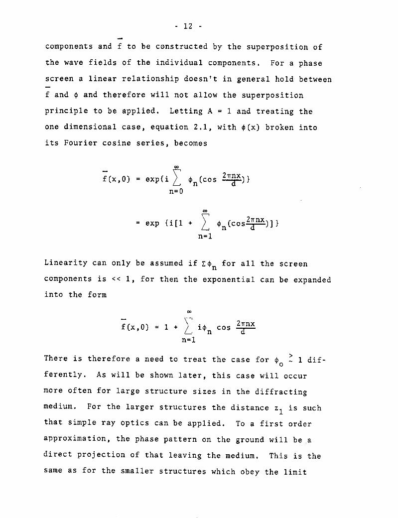
- 12 -
components and f to be constructed by the superposition of
the wave fields of the individual components. For a phase
screen a linear relationship doesn't in general hold between
f and 4 and therefore will not allow the superposition
principle to be applied. Letting A = 1 and treating the
one dimensional case, equation 2.1, with ¢(x) broken into
its Fourier cosine series, becomes
f(x,O) = exp{i n(cos 2n)}n=O
= exp {i[l + n(cos-nx-)]}
n=l
Linearity can only be assumed if Czn for all the screen
components is << 1, for then the exponential can be expanded
into the form
-27rnxf(x,O) = 1 + i n cos -2--
n=l
There is therefore a need to treat the case for ¢o >1 dif-
ferently. As will be shown later, this case will occur
more often for large structure sizes in the diffracting
medium. For the larger structures the distance z1
is such
that simple ray optics can be applied. To a first order
approximation, the phase pattern on the ground will be a
direct projection of that leaving the medium. This is the
same as for the smaller structures which obey the limit

- 13 -
«o << 1, and thus allows a consistent interpretation for
both cases.
For the sake of completeness, the case for Oo q 1
will be looked at in the same manner as that for o0 << 1 to
show the consequences of this limit not holding. Using
equation 2.7 and applying standard phase modulation theory,
f(x,O) becomes:
f(x,O) = (i)nJn(o) exp (2in) 2.12n=-c
--
with F(S) comprising components at S = 0, , . . .
, . ., and amplitudes (i) Jn (o). For n > 4o the Jn ' 0 n
(o0) terms become very small and can be neglected, leaving
2n significant spectral components. The effect of these
higher order terms will be an increased weighting of the
higher components of the power spectrum over what would be
expected from weak diffraction theory. Due to the small
angles of diffraction for these large structures, only the
first few components from a particular point on the screen
will be observed, and the components refracted from other
parts of the screen won't reach the observer. For non-
linear effects of this nature, the presence of more than one
periodic pattern in electron density will not produce simply
additive phase spectra, but will contain also the additional
cross terms for S = m/d1 ± n/d2, where m, n are the orders
of the terms in equation 2.12.

- 14
2.4 Characteristics of the Inhomogeneous F-region
Some important characteristics of the inhomogeneous
F-region must be considered if the phase power spectrum it
produces are to be analyzed properly.
Previous experimental work has determined some
physical properties of the F-region inhomogeneities. By
using spaced receivers, (allowing the construction of a two
dimensional correlation function in the plane of the receiv-
ers) the shape of the correlation contours of the irregular-
ities were found to be ellipsoidal, with the major axis
aligned with the local geomagnetic field. Detailed obser-
vations of amplitude scintillation performed at Boulder,
Colorado (49 degrees N. latitude) produced the following
characteristics (Jespersen, Kamas 1963):
r o = transverse dimension; 0.50 km < ro < 2.90 km; mean
r = 1 km
ANo = total electron variation which increases sharply for
northern latitudes, - 400N.
H = height of the irregularities; mean H = 325 km
T = thickness of the region; T = 120 km
This description is based on amplitude scintillation data,
however, and biased significantly by the diffraction process
as discussed above.
It has been shown (Dyson 1969, Kelleher 1970) that
the irregularities extend to heights much greater than the
average height. It is only because the fairly concentrated
band of irregularities near 300 km produces the greatest
variations in electron density (peak density of the F-region)
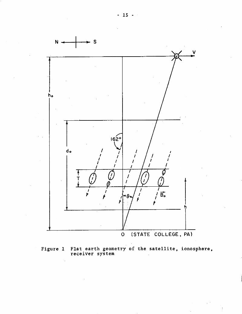
- 15 -
N I - S
0 (STATE COLLEGE, PA)
Figure 1 Flat earth geometryreceiver system
of the satellite, ionosphere,

- 16 -
that the thin diffracting screen approximation can be used.
It is also accepted that the.axial ratio ranges from 1 to
10, with an average of about 3.
Some geometrical.parameters will be brought in now
for later use in Chapter 4. Because.the Beacon.B satellite
is in a polar orbit, the ray path of its signals will sweep
along the major axis of the field aligned irregularities for
overhead passes. At the point of observation, 40°8 degrees
N. latitude, the magnetic field has a dip angle.of 72 de-
grees. For overhead passes the propagation vector k will
therefore be parallel to to (geomagnetic field), for the
case where the satellite is at its southern most point of
observation (zenith angle of = 23 degrees). As the satellite
progresses northward this angle increases to a.maximum of
about 40 degrees. As found by Jespersen and Kamas (1963),
the mean ionospheric height, thickness of the diffracting
medium, and frequency of occurrence of irregularities all
increase with.latitude.
2.5 Diffraction by an Inhomogeneous Ionosphere
Due to the lack of amplitude information in the
recorded data (see Chapter III), it will not be possible to
produce an exact description of the phase power spectra
leaving the diffraction medium, rather a qualitative
description of the general shape of the lower end of the
expected spectra will be sought.
The power spectrum of the phase modulation

- 17 -
P (kx,ky).imposed upon.the:signal near a thin diffracting
screen and:the..power spectrum of.electron .density fluc-
tuations PN(kx,ky,kz = 0) are related by
xy2.P (kx,ky) = 2w(reX) LPN (kxky,kz = 0) 2.11
(Lovelace et al. 1970, Cronyn 1970).
L = thickness of the diffracting.region
r = classical electron radius = 2.83 x 10⁻¹ 5 m
X = wavelength of the signal
kj = spatial wave number in the j direction
kz = 0 was chosen to represent a thin diffracting
medium.
The shape of the two spectra are similar and thus represent
a simple projection of the electron density variations of
the medium on the wavefront in the form of phase fluc-
tuations. It has been observed (Porcello and Hughes, 1968)
that the form of PN for the case of auroral zone inhomogene-
ities can be given by a power law variation of the form:
PN (kxky'kz = 0) = A(kx2 + ky2) -
with BH found experimentally-to range-from 3 to 4.
A check on the validity of the assumption o << 1
will now be made. The-phase deviation in- traversing the
medium is given- by:

- 18 -
= - re ANdl0
where re is the classical radius of the electron. Letting
the deviation in electron density AN be Gaussian, ¢(x) be-
comes (as shown in Briggs and Parkins 1962)
-/-AN r 2O(x) = - reX 0 exp[- ]2x
0
with typical values to be expected
* = angle between So and k = 20 degrees
ANo = maximum electron density change = 1.0% of 10 11 3
9 1 m10109 -3
mX = 1Sm
a = axial ration of the ellipsoid = 5
r = 5 km
O(x) = 8.3 x 10⁻² exp[-2(- ) 2]10
This gives a maximum phase shift of 4(0) = 0.5 radians, It
is therefore conceivable that for larger structures, ro =
50 km, and larger electron density variations ANo = 10%No,
values of 4 could be on the order of 50 radians. Thus we
could expect higher order components along with the first
order term. The number of side components n is roughly
n = p. If we use the value of 109 13 for ANo, the largestm
irregularity for which ~o < .25 radians can be found to be

- 19 -
-2 ro.25 = 8.3 x 10
r = 3.0 km
If it is assumed that ANo is proportional to ro, there will
be a-cutoff at which the approximation o0 << 1 no longer
occurs. It is therefore expected that the power contri-
bution to the high end of the observed phase spectrum will
contain the sum of contributions from the short periodicity
screens and also the higher order components of those large
structures which lie below the cutoff.
Using equation 2.11 the amplitude effects aren't
significant for d >> [2zl(z2/ho)] . For Xz1 = 300 km,
Xz2 = 700 km this condition becomes d >> 3 km to yield a
lower bound on structure size, above which the phase pattern
produced at the ground is a simple projection of the pattern
at the diffracting medium. This cutoff will be chosen to be
5 km.
Due to satellite motion the 2-dimensional spatial
diffraction pattern at the ground has a velocity V = - hiVs/
(ho - hi). Because of this motion an observer at a single
receiving station will observe a one dimensional temporal
scan of this pattern, assuming that it moves without change.
This assumption is equivalent to assuming that the dif-
fracting region is very thin in vertical extent. The
spatial wave numbers of the pattern k. can be equated to the3

- 20 -
temporal frequency components fj by kj = 2rfj/V or
kj = 2rfj(ho - hi)/(hiVs) to produce kj = 2.09 fj sec/km.
The power spectrum in frequency of the received temporal
pattern can therefore be used to reproduce a one dimensional
spatial pattern.

CHAPTER III
SIGNAL HANDLING AND DATA REDUCTION
EQUIPMENT AND TECHNIQUES
3.1 Source and Initial Signal Handling
The source used was the S-66 Ionospheric Beacon-B
Satellite with the following orbital parameters:
Nodal Period 104.8 minutes
Inclination 79.7 degrees
Perigee 890 km
Apogee 1070 km
It produces continuous, harmonically, related
signals at the frequencies 20, 40, 41, MHz (NASA 1963). Use
will be made of one of the circularly polarized modes of the
20 MHz signal and the linearly polarized 40 MHz signal.
The receiving and recording equipment was construct-
ed about 8 years ago by previous workers, with the block
diagram shown in figure 2. The data was collected over the
period 1964-1968, and after processing was stored on mag-
netic tape. The signals were also recorded on chart records,
a sample of which is included in Appendix B. By using har-
monics of a single tracking oscillator for both frequencies,
the phase relationship between them was preserved for later
phase comparison. The receiving antennas consist of a fixed,
vertically directed, circularly polarized.antenna and a
fixed dipole with an east-west orientation.
The direction of polarization of the incoming
C-

- 22 -
a~~~~~~~~~N1:
N5
NZI
Er
0LLN J
I
o
I >
N l
W
o
I 0
1
Z-
u
u0
0-cz Z -UJ
aF-I w
IL D2
I I
ItgwH:
qZJ
owOW-
0L-
N
00L.L
I
NWIW
OI
a
a)
a)4 J0
o
CUc,1
.rq
a)
bo
VL.
m
.H,
0
u0
4J
440
O
.rH
u,

- 23 -
signals will change with time to produce a.Faraday rotation
rate. This is caused by the systematic change in.iono-
spheric thickness and in the.longitudinal component of the
earth's magnetic field with zenith angle. For the single
dipole antenna this produces severe amplitude variations
which must be compensated for in the early stages of the
electronics due to the critical signal level.dependence of
the phase detection circuitry. There will also occur phase
discontinuities at the times of cross-polarization between
the incoming wave and the antenna. These discontinuities
will produce spikes in the temporal.diffraction pattern
and therefore produce a spurious addition to the phase
spectra. Because the 20 MHz circularly polarized antenna
was fixed it will appear to be ellipitically polarized for
oblique incidence of the signal. This will produce an
apparent, non-uniform Faraday rotation rate which in turn
produces phase modulations. The magnitude of this effect is
increased with increasing zenith angle which makes necessary
the limiting of satellite longitudes to the range 75-80
degrees west and of latitudes to the range 35.5-46.5 de-
grees north. Since the above effects.are reduced by a
decreased Faraday rotation rate which is dependent on the
integrated electron density of the ionosphere, only night
time records will be used.
A brief note will be added here as to why linear;
rather than circular polarization was used for the 40 MHz
signal. Both 20 and 40 MHz circularly polarized signals

- 24 -
were stored on the same tape channel. There was some dis-
tortion in the receiving equipment which generated a second
harmonic of the 250 Hz stored signal. This harmonic was
inseparable from the 500 Hz signal, and caused spurious
phase modulation of it.
3.2 Analog Processing
The approach used is to compare the frequencies of
the two previously stored signals yielding a continuous
temporal frequency record. This represents the derivative
of the temporal phase function w.r.t. time recorded at the
receiving station. The frequency record represents the
deviation w.r.t. time of the signals from their harmonic
relationship, which will give the phase path difference
experienced by the signals in traversing any inhomogeneities
in the F-region. Utilization of harmonically related sig-
nals allows the elimination of tracking errors, source
stability errors, and phase noise induced during the record-
ing and playback process. This is accomplished by frequency
doubling the 250 Hz signal and comparing it with the 500 Hz
signal to eliminate any modulation proportional to frequency,
of which all the above produce. The 500 Hz signal was off-
set by 180 Hz (chosen by trial and error to produce the
least harmonic distortion) to facilitate phase detection. A
block diagram of the electronics is shown in figure 3, where
C.f. and B.W. are abreviations for center frequency and band-
width respectfully. The following requirements were placed

NIO xo0
CLu
, N
w -
L. -O
<9 NW1
I D I
LL
N N
z c m
>
NI0ot >.co(D
_ .
NN
/ ii
X t
II
z o
_
CL
& o m- 11-L
U- : 3
T1
Iahi
o a
. < 0
i I
- 25
-4--
U*rl
U
e$4
C,
4
rS
b0
U
'.4
C:S
ba
br4
.14

- 26 -
on the electronics to account for physical conditions and,
or previous recording methods.
Because the frequency discriminator used was
sensitive to amplitude variations, severe amplitude limiting
was imposed prior to frequency detection. This need was
made more demanding by the deep nulls in signal caused by
Faraday rotation, especially on the 500 Hz signal.
Predetection bandwidth requirements were imposed in
early limiting to prevent harmonic distortion from reaching
the frequency detector. Minimum bandwidth (B.W.) require-
ments are set by the phase modulation induced on the signal.
Due to the changing effective thickness (shown in figures 1
and 4) of the ionospheric layer with satellite latitude a,
we will have a linear ramp imposed on the discriminator out-
put. Hereafter this effect will be referred to as the
apparent doppler dispersion. Its magnitude is approximated
by:
* = -reX N(x)dx 3.1
1 d reXdf 1= d = re Ndx 3.2
r Xrex d= - 2· (No) 3.3
No= average electron density (assumed here to be constant)
k = arbitrary ionosphere thickness

(a)
Sln [IT
-300
(b)
-300
Figure 4
oan - (Vs R/18ho)]
vs. ,
,,mi~~~~
- 27 -
I 300
I
.1 2
vs. P f(/3)= SlnP[CosI(r,+r 2 - r CosI)-rr][l-
(Sln2P/ r 2 +r2 - 2rr, CosP)] '
PMI .I
Frequency modulation caused by the apparent dopplerdispersion for (a) flat earth, (b) curved earthgeometry. R radius of the earth, r - (R + h.)/(R + he, rle = (Re + hi)/Re, aM = maximum Beofobservai on
- 28 -
and becomes
r df = - .XNV 0- sin 8 3.4
0
The records were restricted to values of e - 8m =
230. Using nighttime values of No given by Solomon (1965),
the maximum frequency deviation for the frequency doubled
250 Hz signal at the extreme zenith angles of the data was
found to be fmax + 0.5 Hz for the 20 MHz signal. Because
both the 20 and 40 MHz signals are modulated by the iono-
sphere similarly but with different magnitudes, 20 - X40
should have been used rather than k20 which reduces fmax to
about ± 0.4 Hz.
The tracking errors were measured by previous
workers to be as large as 10 Hz and must be considered in
B.W. considerations of the filtering prior to the mixing of
the two signals. Because the analysis treats ionospheric
induced frequency modulations up to 3 Hz, (actually up to
8 Hz, but this region wasn't analyzed because of severe
attenuation due to postdetection filtering) this will have
to be added into both predetection and postdetection B.W.
limits. Combining the above, the predetection B.W. needed
is 2(10+3+0.5)Hz = + 27Hz. It was set to 30 Hz. Post-
detection integration contained a cutoff at 2 Hz.
The discriminator output represents the frequency
difference of the 2 signals as a function of time. This
necessitates that the delay of each signal through the

- 29 -
electronics be identical, i.e., that the rates of change of
phase shift vso frequency for each signal channel be equal.
This was achieved with an additional filter in the 250 Hz
channel to yield slopes differing by less than 5%, repre-
senting a phase error of ten degrees for a frequency change
of 28 Hz.
Because the discriminator used was very sensitive to
amplitude variations, severe limiting was used and signal
amplitude was monitored to insure against fluctuations.
Discriminator output remained constant for the following
ranges of signal input:
Amplitude 250 Hz: 0.6 - V(250) - 3.2 VP-P
Amplitude 500 Hz: 0.2 - V(500) - 3.2 VP-P
The discriminator output was placed through a 3 stage, low
pass, filter with cutoff at 2,0 Hz.
Its response was linear over the range used (± 5 Hz)
with a sensitivity of 2V D C and a noise level (due primarilyHz
to intermodulation in the earlier electronics) of ± .02 Hz.
A sample of a typical chart record produced by the
above is shown in figure S. This information consisted of:
Channel 1: WWV
Channel 2: discriminator output f(t) in Hz
Channel 3: discriminator input amplitude monitoring
Channel 4: 40L amplitude monitoring
3.3 Data Analysis
The aim of this stage of analysis is to obtain a
- 30 -
·I ·~~~~~~~~~~~~~~~~~~~~~-_ ~ n-*~ ri 117 L_ _ 1
t ._7>tl-l =S1 . .,,.. -- -. .. -._ ...._
t ::j it i::: i;:.~~~~~:
Lir ~ ~ ~ ~ ~ ~ ~~i.
It=:
4j.
- - -- -- -- Li -7 ::7-~~~~~~~~~~~~~~~~~~ ···
1 1 i! -':41- 1 - 1-! 1 ::-1 1>:-1--1 --- t :-''- "-'~'~-·~·'--· -_ *- p-l~- - --'~'"~"-··'·-k-:::I f
j~~~~~~~~~~~~~~- ci)
tf)
.... ·· ','s <'-- WObO
k, -. 1,~~- --~ IF
tt-' |' - | - 1 ' - | -' ' | : | ! ;$~~~~~~~~~~
1=01tX~~~~~~tX 3Xm-0X--'0~~_L 7 L,- -[" taL -.L5 t
j: :~~~~~~~~~~~~~~~~~~~~~~~~~L: L . :
2 1 S :L W l gL l l X l i, E~ : t - l -k: l= { ;i i l .;t<h2
-=-jFU Ft mE---E- --E 1Er _4i f t H - "I z
1O
7.$~~~~~~~~~~~~~~L1~~. .. H 5 ·
-- -i , ;
-V~~~~z- ~ -:Lt" t4 77iii~
xi~~ - i 1k
+~~~~~~l-
mr- ~ ~ ~S ·:: -- - ··· - ii:~~~~~~~~~~~~~~~~~~~~~~~~~~~iiZ -i'
Lo zt=~-~-- ~-·--~- -I~i 17_·LiT~I1 ~ - ---- (.:P.·- ~-..11~ r-a

- 31 -
power spectrum of.the phase variations.imposed on the
received signal. The method used is outlined.by Blackman
and Tukey.
To avoid the complexity required to obtain the
frequency.components by analog.,methods, .the data will be
digitized.. This action replaces the.continuous function
f(t) by f(tj), where tj represents the discrete time values
jAt, j = 1,2 . . . N, NAt = length of the record. As noted
earlier, there exists a D.C. trend on the data. To elimi-
nate this large,.low frequency contribution, the best linear
fit line was.subtracted from the data point by point. De-
termination of the line defined by the quantity (a + 8jAt)
was achieved by the use of:
N
Z [f(t) - a - B1] = 0 3.5
j=1
N
(j N) [f(t) - a - j] = 0 3.6
j =1
Solving for a and 8, the trend and mean can be subtracted
out. The autocorrelation function of the detrended data
was found, and its Fourier transform taken, yielding the
power spectrum in frequency, which will be shown later to be
related to the power spectrum in phase. Several aspects of
digitizing data must be considered before the usefulness
of the data can be assured.
Computation was performed on a PDP-10 digital com-
puter with a limit of 23 k user available core. This set

- 32 -
a practical upper limit on the size of the data array and
therefore the sampling rate. Because the maximum observable
frequency with a sampling rate of N per second is 1/(2N), N
was set so 1/(2N)=8 Hz. The data was already limited to
3 Hz due to final filtering, so no loss of information
occurred. N therefore is equal to 16 samples per second.
Previous work (Porcello and Hughes, 1968) has shown the
power spectra to fall off with increasing frequency which
will further reduce aliasing. The longest lags obtained are
determined by the length-of the record, and are usually
taken to be 5-10% of the record length. We chose lags up to
32 seconds which is = 16% the record length, This gain in
range of data is seen in-equation 3.7 to reduce the stabil-
ity of the results (represented by K).
Maximum aliasing is determined by the attenuation of
the output filter. The power at the folding frequency of
8 Hz is compared with that at 0 Hz and was found to be down
68 db. This is more than sufficient to eliminate any
aliasing problems.
Due to changing ionospheric conditions between
orbits, nonstationarity between records is assumed, which
forces statistical independence of the records, rather than
an average over an ensemble. For the record length avail-
able and maximum lag used, the number of degrees of freedom,
K, is found to be (Blackman and Tukey):
2Tn' 2[Tn 1/3Tm]
K = _r_- T 'T3.7m m

- 33 -
Tn
= total record length
Tm = maximum lag desired
K = 11-1/3. Use of Table II in Blackman and Tukey leads to
an 80% confidence limit of 4.8 db. This value is only
characteristic of the runs taken, with.exact values given
later for individual records.
Past evidence (Porcello and Hughes, 1968) has shown
the phase spectral density to follow a power law relation-
ship, given by
BH+ 1
P[(kX ,ky ) (kX 2 + ky )
with kx, ky the wave numbers and SH an experimentally
determined variable. This indicates the need for pre-
whitening, The data being originally.intended for other
uses, prewhitening wasn't performed. This will reduce the
signal to noise ratio.,at the high end.of the spectrum,
making that region more susceptible to interference or noise.
The process of taking a finite sample is equivalent
to multiplication of the infinite data set with a square
pulse. This will accentuate the high frequency end of. the
spectra. This effect was reduced by passing the auto-
correlation function C(Tj) through.a Hamming spectral window
D(Tj) where
D(Tj) = ° 54 + .46 cosrTj/Tm) ITj I < Tm
=0 ITj > Tm

- 34 -
The attenuation due to final integration was compensated for
by direct measurement of the characteristics of the low-pass
filter and multiplication of the frequency power spectra
lines by the appropriate value.
The flow diagram and computer program are included
in Appendix A-2.

CHAPTER IV
EXPERIMENTAL RESULTS
4.1 Experimental Details
The individual orbital conditions.and,statistical
parameters of the data used are given in Table I. Due to
the severe.limitations on longitude and the restriction to
nighttime records, only a small fraction of the available
library of records was considered of which only 8 satellite
passes produced significant frequency variations observed at
the discriminator output. The effectiveness of the trend
removal performed on the digitized.discriminator output was
about a -106 reduction in mean value, and a 107 reduction in
slope. Because both the original mean and trend were of the
same order of magnitude as the desired information, these
reductions brought their effect well below the noise level.
For an 80% confidence limit, there was typically a 5 db un-
certainty range in the relative power spectra.
A sample of the discriminator output is shown in
figures. The 40 MHz amplitude channel was displayed so
as to observe the magnitude of the frequency spikes produced
by the Faraday rotation and any possible amplitude effects
it could cause. These finite width spikes have a minimal
overall effect on the spectra-due to their infrequent occur-
rence. .The scale is 1.0 Hz per division on the discrim-
inator channel.

/i ·'.
- 36 -
C °Q % VD Ln ".
oo Ioo u
*1-4 00 ,'D 4-) t tC- 0) r :t C' l It
a , sq -d- t vn tn q a tnu) bo 0 rq ro - . .. ..U)~ b O *H·
H g 4-4-H 44 t U") U") Ln) .- d l
U) o L)
P4 :
¢ o
·a~2 C) -tn 0, r-I 0) 0) C0-4 O O -4o -I o o u- - -I
p: Z 00 ,
U) C') 4 1
(; F'4 U) - q v- r-I r4
4 i
H 4~b'4 a) te) 00 cc 00 lq- \0 0)HI *v-4+G) . . ..
gC bo c 0 o o -i C o 0 0 0) 'dtrl U co 00 0c r- 00 r- t-. t-
0 00z _r , < . . . .4. .C.
E IC: ' * 0 U a Cm-1r 4i t-I -1 \'- 0t \' a -I v-I tn
1H0 N 0 O O 0 C N N
4c \0 n cc 00 0 \0 1- N-H - '0 r- r- '0 Id U") 0) '0*,0 Lf ,-4 ) q Lf" t) C 0 ),
h Z O 'o 0 o cc 0) 0) LuO v-

- 37 -
4.2 Spectral Density of the Frequency Modulation
(a) Analysis of the high end of the spectra.
Sample plots are shown on log-log scales in figures
6-11, Figures 6 and 7 show a spectrum before smoothing and
after smoothing, Smoothing was accomplished by taking a
running average over three unsmoothed logarithmic spectral
values, which themselves were arithmetic averages over two
adjacent spectral values. The remainder o.f the figures are
for smoothed plots only. This doesn't reduce the useful
information because as is seen in figure 6 the features pre-
sent in the unsmoothed version and not in the smoothed
version are within the range of uncertainty imposed by the
80% confidence limit shown on each graph. The consistent
appearance of nulls at the high end.of the spectra is a
feature to which attention is now drawn.
For a source at a finite distance from the observer
it was predicted in equation 2.10 that nulls in the power
spectra of structure sizes should occur for dimensions
given by equation 2.11. A conversion from spatial to
frequency spectra produce nulls for frequencies
V h. Vho V 2n h.f = i h i = v .)) n 12 .
oD xU 2Fh4(h°0 0 0 0 i
4.1
This produces nulls at the frequencies (for n = 1,2,3,
respectively) f = 0.675, 1.31, 1.69, . . o Hz, Figures
6-11 show definite nulls in this frequency range, but

- 38 -
---- 83MOd 3AI.V1 138-
'
, . 4
I%So · ··
wzw
LL
00
o
00
0
. . ..
. ..
., ·
wUz
0Z
z0
0o
a:)00
o
4-
0
0.4-4
N U
>4
U
O
W 0
- C)0 r
I- o
:1)25
to
a w
0 P4o~~~~~~~~a
0
N- m
U
wZ
0
LLA0
4 J.-,.4
0
s40
4 -4
r::
4.JUa)Pw(n
q)
0
C)
q)n 4-)0
9,'-4
000.0
000.
000.0
00q
I I I
m_ O_oII

.I. .I
. 0
· wUzw
Oz
oC-
0
·O c4'.4
0
0,
I 4
I..
- aP4
> 0Z 0w ro=)
LL Lc ,0
C hrvl L
_ o-0
C0
.4
L.,
0-I
I -
.$ e
w
z0L)
Ol'0
0
4-i.O,
·.4
0
0
O
O4-4
N .-I ':
4J
Uu
z
o. ',!0w
4)
~ OOt
U? ,-4
oo
00s4
04
- 39 -
000~0
O
oc
O0.
0 O
000.0
000
Ii,
00
0 -ci
I
----f 83MOd 3AILV13
I I I
I

- 40 -
·--- 83MOd 3AI11V38 -
I ·
* .
%;
wUzw
o
aoz
OD -
OO0O
OOm
0
*'.C'·. ®e
Uz
a
z0
00OD
00o
m
00
0
.,-0 .0
0
1.40
N U
o
U )zW 0o
Wo 4
0 m
Etn
uoo
V a%
r-4
Z $
O5 4
6 W
O
NI
>-UZ
DO
O W
_I
p4.,..0,z40o
0o
a)4
(n
o$
a)
P4
a)
o
,-
bO
p4
0
0§
00
0dr
I I
1

- 41 -
generally not at these precise values.
Upon a closer analysis of the geometry involved, it
becomes clear why the predictions above aren't realized.
The values of the predicted nulls depend on the height of
the diffraction medium and the distance to the satellite.
As shown in section 2.4 the medium height increases with
increasing latitude and h0 increases with zenith angle. The
finite thickness of the diffracting layer also produces
inhomogeneities at different heights. Assume for example
that hivaries over the range 300-400 km. This produces a
first order null ranging from 0.675 to 0.504 Hz to produce
a broad null centered about 0.59 Hz. It could also be the
case that there exist diffracting layers at different
heights. This effect could come about through a patch
structure of inhomogeneities as observed by Kelleher and
Sinclair (1959). Here structures appear in groups pro-
ducing the possibility of patches occuring at different
altitudes, 300 and 400 km for example. This would also
produce distinct first order nulls at 0.675 and 0.504 Hz.
No quantitative analysis will be made of this region
for the following reasons: (1) the confidence limits are of
the same order of magnitude as the depth of the nulls,
(2) the data is believed to be approaching the system
noise level in this region as indicated by the character-
istic flattening of the spectra. Had these two conditions
not been present, some estimate of the height and thickness
of the diffracting medium could possibly have been obtained

- 42 -
from the position and.shape.of.the.nulls. It is interesting
to note that.although.the nulls should occur in both
amplitude and phase-power spectra, amplitude studies
(Rufenach 1972) have only rarely observed them, while they
are quite evident in this study using.phase scintillation.
(b) Analysis of the low end of the spectra.
This is the region of the spectra containing fre-
quencies below the first null. This frequency is found,
using equation 4.1 for n = 1 and converting from normalized
distances to actual distances, to be
f = I m XA] = Vs[( 2) z 4a20 2 a
It is in this region that some insight might be gained as to
the physical nature of the diffracting medium.
From the records studied there tends to be a definite
slope 8 in the log-log plots shown, This would indicate a
frequency power spectrum of the form
P(f) - (f) 4.2
Upon taking a visual estimate of the slope, it was found
to have a mean value of 0.71 and standard deviation of 0.10.
These values were found neglecting the B value for orbit
10566 due to its large.deviation from the norm. Upon look-
ing at the chart record for this run a considerably larger
amount of low frequency variations were.present, thus

- 43 -
indicating.a greater than average (taken over the 8 passes
used) number of larger structure.sizes.w.ort. the smaller
sizes.
(c) Statistical stationarity of the results,
Due to the similarity of values of S.for the dif-
ferent orbits, some support is rendered to the case for
statistical stationarity of the medium wor.t this parameter.
Porcello and Hughes (1968) also..found similar values for $
for structure sizes smaller than considered here. From the
limited sample taken, there is the indication that the
parameter is a characteristic of the medium and not depen-
dent upon temporal changes occuring in the inhomogeneous
makeup of the diffracting medium. Orbit No. 10566 produced
a 8 value with considerable deviation from the mean value.
Because of the limited sample taken, no conclusions will be
drawn from this deviation.
4.3 Discussion of the results
It was shown from the graphs and expressed in
equation 4.2 that the power spectrum obeys a power law
variation with frequency. What is of more physical signi-
ficance is the power spectrum of the phase difference c(t)
of the two signals, Noting that f(t) = dp(t)/dt, the
Fourier transform of f(t) is
00
Ff(f) = f(t)e 2-riftdt

- 44 -
co
Ff(f) = Pt d (t)e 2if tdt
1 f (.t) e 2 iftdt-00
= - ifF (f) 4.3
the comparison of power spectrum yields:
Pf(f) = IFf(f)12 = f 2 IF (f)2 = f2p (f)
P (f) = f-2Pf(f) 4.4
P(f) f-(8 +2 ) 45
It is now desirable to determine the nature of the spatial
power spectrum in phase leaving the diffracting screen,
denoted by Po'(k). Equation 2.8 shows how the angular
spectrum in phase changes as the distance from the screen
increases. For the cosine diffracting screen considered
previously, the power at the screen is given by
P (S) = IF(S) 12 = 1 + o2 ( S = d)
On the ground the power contained in the phase part of the
angular spectrum is
P' (S) = IG(S)I 2 = o2cos2 [2r(1 - - - 1)z](S =

- 45 -
Po'(S) = o 2os2rS2 z 4.6
Expanding the cosine term P,' S) becomes
IP '(S)I 4 )2(1 - zS2 ) 4.7
Because it has already been assumed that zS2w << 1, the
spectrum is independent of S and identical to that for
z = O. Next the dependent variable in equation 4.5 will be
changed from frequency to wave number along the direction of
motion k using k - f
-($+2) 4.8P (k) ak(+ 2 ) 4.8
A proportionality rather than an equality is used due to the
nature of measurement of the power spectra. The power
spectrum of the electron density fluctuations is therefore
PN'(k) Q k (+ 2 ) 4.9
What is obtained therefore is a power law variation
in electron density fluctuation over the range of iono-
spheric structure sizes 5.0 km to 73 km. The character-
istic exponent was - 2.71. Previous work by Rufenach (1972)
found using amplitude scintillations, that 8 ranged from
0 to 1 for structure sizes 0.6 to 4 km. Using phase

- 46 -
variations Porcello and Hughes (1968) found 1 for 2 records
to be 0.8 and 1.0 for auroral conditions.

CHAPTER V
SUMMARY
5.1 Conclusion
A study was made of the inhomogeneous nature of the
nocturnal F-region from a ground station at 40.80 N. lati-
tude using phase information from two harmonically related
satellite signals. A phase comparison of the two signals
eliminated tracking and processing errors common to both,
but not the dispersive ionospheric phase modulation. From
the phase modulation of the signal, the power spectra of
the electron density variations in the diffracting medium
(of wavenumber k) was found to follow a power law relation-
ship PN (k) = k- ( 8 + 2 ) Values of $ were found to lie in the
range 0.50 to 1.5 with a mean of 0.71 and standard deviation
of 0.10. Because of experimental constraints, this expres-
sion could only be verified over the range of structure
sizes (2r/k) from 5.0 to 73 Km.
What is believed to be Fresnel oscillations was also
observed in the diffraction pattern. The characteristic
nulls in the power spectra of phase variations were present
at near the expected frequencies, but due to experimental
uncertainties no detailed analysis was performed on them.
Statistical stationarity of the medium w.r.t. the
parameter B was considered. Because of the small standard
deviation of this value, the exponent - (8 + 2) appears from
the limited sample of ionospheric conditions observed to be
'L1

- 48 -
a characteristic of the inhomogeneous F-region. One orbital
pass did yield a value for a of 1.5, but further measure-
ments would be necessary to examine its significance rela-
tive to the above stationarity.
The advantage of the use of phase over amplitude
information was made clear by the direct interpretation
given here to the data in terms of parameters of the dif-
fracting medium. Amplitude studies have the problem of
interpreting the effects of diffraction, as do phase studies
for structure sizes below a cutoff value. It is the larger
structures which allow observation in the near field and
are therefore without major diffraction effects.
5.2 Suggestions for Further Work
This study of the spatial power spectrum of electron
density fluctuations in the ionosphere has been constrained
in several ways by experimental limitations, and the method
could be improved by easing these conditions.
For the smaller scales, less than a few kilometers,
diffraction effects complicated the interpretation of data.
The use of higher frequencies would extend this range and
would also reduce the depth of phase modulation in the iono-
sphere and thereby lead to a more direct relationship be-
tween the diffraction pattern and the medium. However,
unless the system noise level could also be reduced for
example by the use of higher powers or higher gain (tracking)
antennas, and improved recording methods, the extended

- 49 -
range might well be lost in noise due to the lower sen-
sitivity of the effect on higher wave frequencies.
For the large scale end of the spectrum the study
has been limited by the finite length of record which can
be obtained in the limited field of view of a receiving
station. Although some small extension of the range
(perhaps a factor of two) might be possible through the use
of tracking antennas, this would introduce greater changes
in the experimental geometry and further complicate the
analysis.

BIBLIOGRAPHY
Appleton, E. V., and M. A. F. Barnett, Local Reflection ofWireless Waves from the Upper Atmosphere, Nature, 115,333, 1925a.
Blackman, R. B., and J. W. Tukey, The Measurement ofSpectra, Dover, 1958.
Briggs, B. H., and I. A. Parkin, On the Variation of RadioStar and Satellite Scintillations with Zenith Angle,J. Atmospheric Terrestrial Physo, 25, 339, 1962o
Cronyn, W. M., The Analysis of Radio Scattering and SpaceProbe Observation of Small Scale Structure in theInterplanetary Medium, Astrophyso J., 161, 755, 1970.
Dyson, P. L., Direct Measurement of the Size and Amplitudeof Irregularities in the Topside Ionsophere, J. Geo-physical Res., 74, 6291, 1969.
Elkins, L. J., and M. D. Pagagiannis, Measurement and Inter-pretation of Power Spectrums of Ionospheric Scintil-lations at a Sub-Auroral Location, J. Geophysical Res.,74, 4105, 1969.
Herman, J. R., Spread F and Ionospheric F Region Irregular-ities, Rev. Geophys., 4, 255, 1966.
Jespersen, J. L., G. Kamas, Satellite Scintillation Obser-vation at Boulder, Colorado, J. Atmospheric TerrestrialPhys. 26, 457, 1964.
Jones, I. L., Further Observation of Radio Stellar Scintil-lations, J. Atmospheric Terrestrial Phys., 19, 26, 1960.
Kelleher, R. F., and J. Sinclair, Some Properties of Iono-spheric Irregularities as Deduced from Recordings ofthe San Marco II and BE-B Satellites, J. AtmosphericTerrestrial Phys., 32, 1259, 1970.
Kuntman, D., A Method for the Determination of Mean Iono-spheric Height from Satellite Signals, ScientificReport No. 278, Ionosphere Research Laboratory, ThePennsylvania State University, August 1966.
Lovelace R. V. Eo,-E. E. Salpeter, L. E. Sharp, Analysis ofObservations of Interplanetary Scintillation, Astrophys.J., 159, 1047, 1970.

- 51 -
NASA Goddard Space Flight Center, Polar Ionospheric BeaconSatellite (S-66), X-533-63-29, 1963.
Perelygin, V. P., Geomag. Aeron., 9, 281, 1971.
Porcello, L. J., and L. R. Hughes, Observed Fine Structureof a Phase Perterbation Induced during TransauroralPropagation, J. Geophysical Res., 73, 6337, 1968.
Ratcliffe, J. A., Some Aspects of Diffraction Theory andTheir Application to the Ionosphere, Reports on Progressin Phys., 19, 188, 1956.
Rastogi, R. G., H. Chandra, M. R. Deshpande, Drift andAnisotropy Parameters of the Irregularities in the Eand F Regions of Ionosphere Over Thumba During 1964,J. Atmospheric Terrestrial Phys., 32, 999, 1970.
Rufenach, C. Lo, Power-Law Wavenumber Spectrum Deduced fromIonospheric Scintillation Observations, J. GeophysicalRes., 77, 4761, 1972.
Solomon, S. L. Variations in the Total Electron Content ofthe Ionosphere at Mid-Latitudes During Direct Sun Con-ditions, Scientific Report No. 256, Ionosphere ResearchLaboratory, The Pennsylvania State University, November1965.
Spencer, M., The Shape of Irregularities in the Upper Atmo-sphere, Proceeds. Physo Soc. A, 211, 351, 1955.
E

APPENDIX A
1. The following program was used to take a con-
tinuous signal and sample at a uniform rate to produce a
data array for digital analysis. The sampling was control-
led by a D.C. level on a separate channel of the tape re-
corder. The comparator (number 34 referenced in lines
170,200 of the program) sensed when the level was + 1 or 0
VDC to control the interrupt subroutines. The comparator
was fed into an 'AND' gate along with the clock set at 16
pulses per second. The output was then fed to interrupt
0 (referred to in line 80). The data was fed into the A/D
converter channel 0 (referred to in line 230). The data was
stored on Dectapes under the file names TEMPl1DAT,TEMP2.DAT
etc. in arrays A(4100).
2. The flow diagram in figures 12, ]3 is intended
as an outline of the method used in data handling and not
for use in detailed programming. The following Scientific
Subroutine Package programs were used.
Auto: calculates the autocovarience of the data array A
RHARM: calculates the Fourier coefficients of the real
data array A.

- 53 -
REAL A(4100)LOGICAL RSCSINTEGER A2(8)INTEGER A1(4100)EQUIVALENCE (A,A1)EXTERNAL ICRACDO 100 1=1,8CALL HINITCALL GPI(0,IERR,ICRAC,0,4100,A1)CALL STINT
C START AN ALOG: SET MODE CONTROL TO OP,RUNCALL SAMO('OP')TYPE 1000
1000 FORMAT('START RECORDER',$)ACCEPT 1001,IANS
1001 FORMAT(I)CALL SLIMO('RUN')
105 IF(RSCS(034)) GO TO 110GO TO 105
110 CONTINUEIF(RSCS(034)) GO TO 110CALL GPISTA(0,.TRJE o, RETURNI, 4100, 1 DEX)TYPE 500
500 FORMAT'(''DECTAPE FO. FOR OUTPUT?',$)ACCEPT 501,MNDT
501 FORMAT( I)NDT-NDT+8GO TO (1,2,3,4,5,6,7,8),1
1 CALL OFILE(NDT,'TEMP1t)GO TO 9
2 CALL OFILE(NIDT,'TEMP2')GO TO 9
3 CALL OFILE(NDT,'TEMP3')GO TO 9
4 CALL OFILE(NDT,'TEMP4')GO TO 9
5 CALL' OFILE(NDT, gTEMP5')GO TO 9
6 CALL OFILE(NDT', TEMP6G)GO TO 9
7 CALL OFILE(NDT,'TEMP7')GO TO 9
8 CALL OFILE(I;DT,'TEM1P8')9 WRITE'(NDT' 10') INDEX, (A1(')', J=1, INDEX)10 FORMAT(' ',T40,15/' ',20(1X,15))
'A2(1)=INDEX100 CONTINUE

- 54
REAL A(4100),R(512) ,COEFIC(50)DATA (COEFIC'(J) ,J=1,50/50 VALUES/
.rREAD(FROM DECTAPE)
INDEX-,A(J),J=1,INDEX
X1=X2=0K= (INDEX-1)/2
IYES
X3=INDEX
I
J=1J=J+ 1
IS J INDEX
X2=X2+A(J)X1=Xl+J*A (J)
I X4=-(X3*X3-1)*X3/12X5=(X2+1/X4*(X1-.5*(X3+:1)*X2)*.5*X3*(X3+1))/X3X6=-(X1.-.5*(X3+) *X2)/X4
YES J=1J=J+1
IS J X3
INO
I A(J)=A(J)-X5-J>*X6
0 CONTINUED FIGURE 14
FLOW DIAGRAM OF DATA ANALYSIS PROGRAM.
rI
FIGURE 12

- 56
APPENDIX B
j - - - - - :"#i: glE'lti igl .410: 01...| ... - X i
: k: :! I ::1I . ' ' . : I -: : i _ . - '- '
. _ _ _ _ _ _ ._ T _ _ _ i --- T i,! = _ _ _ _. . _ , . _ .f
I i~ ~ ~ ~ ~ ~~~Q-
I~~~~~~~~~~~~~~~~~~~~~~~~~~~~~~~~ a)
i ~~~~~~.. .. ..,,. .. -) -- -'103 I _ . .. ... .. ._ . i - i:, A
w -w . -t~S~tS~171 i,.1-N1'i -- -ik -,1 --t:10':;
lui~u
1:: a -t 1 -tl | | ~101i ptif 1 : E |
p::~~~~~~~~~~~~~~F
21L I i - :8::1 1 1- N-17: .o L {W-W< J== i;; e.1-ll-8-;''l-1:~l> d
"L.; li e I T7--_ ,,.
pp. 1 1 g1 -X-1
~~~dk~ ~ ~ ~
r:~ ~ ~ ~~~~k-
T| 141 1 1 1 : 1 < > b1 ! 1. I ih~~a
IlM~~lLE t]_Lt z Mcb
d : Jd11:51' 11001 1$f~vt1:l' XC~dO tS t::~ t! 0 | mE 4> in
1: :fsz l lie~l-i slb~lil: s~i i* :i iiFk
A~fgt0!01- iS10l$10g101l --0010!40- | ra,
v;":Ei~lr ~l:!E.ggi':'t!ilt~l -i~g! l l II l = WO I:rmll:l .Ig~x ri .l:ll,1:l: --. EE+ : r 1 i| J
'IN4I~hliS'!I!I ' I;iE.4IifI4. I0[ t :111~~~~~~~~~~~~~~~~v 1 izl 11rIl,l.igIiIli1i 11LlhI
'i1L#11 11-4it1 4 1 l _ l,,ll:-1g1 : 1:1:1 1ri
.iltillf' l + ililil""l l~l - L= _ X
" | t[1 Siil |iliSlilti l~ i~
55
CONTINUED
L=NUMBER OF LAGS DESIRED=512TM=MAXIMUM LAG IN SEC.=32.0T=SAMPLE PERIOD IN SEC.0.0625M=IMPUT PARAMETER FOR RHARM=8
YES
YES
FIGURE 13. FLOW DIAGRAM (CONTINUED)


