
pst-labo-docEN - BaKoMa TeX · Title: pst-labo-docEN.dvi Created Date: 10/16/2005 10:54:55 AM

1000 (34.5%)
500 (17.2%)
600 (20.7%)
450 (15.5%)
150 (5.2%)
200 (6.9%)
Taxes
Rent
Bills
Car
Gas
Food
PSTricks
pstricks-add
additionals Macros for pstricksv.3.31
April 29, 2009
Documentation by Package author(s):
Herbert Voß Dominique Rodriguez
Herbert Voß

This version of pstricks-add needs pstricks.tex version >1.04 from June 2004,
otherwise the additional macros may not work as expected. The ellipsis material
and the option asolid (renamed to eofill) are now part of the new pstricks.tex
package, available at CTAN or at http://perce.de/LaTeX/. pstricks-add will for
ever be an experimental and dynamical package, try it at your own risk.
• It is important to load pstricks-add as the last PSTricks related package, oth-
erwise a lot of the macros won’t work in the expected way.
• pstricks-add uses the extended version of the keyval package. So be sure that
you have installed pst-xkey which is part of the xkeyval-package, and that all
packages that use the old keyval interface are loaded before the xkeyval.[1]
• the option tickstyle from pst-plot is no longer supported; use ticksize in-
stead.
• the option xyLabel is no longer supported; use the option labelFontSize in-
stead.
• if pstricks-add is loaded together with the package pst-func then InsideArrow
of the \psbezier macro doesn’t work!
Thanks to: Hendri Adriaens; Stefano Baroni; Martin Chicoine; Gerry Coombes; Ulrich
Dirr; Christophe Fourey; Hubert Gäßlein; Jürgen Gilg; Denis Girou; Peter Hutnick;
Christophe Jorssen; Uwe Kern; Manuel Luque; Jens-Uwe Morawski; Tobias Nähring;
Rolf Niepraschk; Alan Ristow; Christine Römer; Arnaud Schmittbuhl; Timothy Van
Zandt

Contents 3
Contents
I. pstricks 7
1. Numeric functions 7
1.1. \pst@divide . . . . . . . . . . . . . . . . . . . . . . . . . . . . . . . . . 7
1.2. \pst@mod . . . . . . . . . . . . . . . . . . . . . . . . . . . . . . . . . . . 7
1.3. \pst@max . . . . . . . . . . . . . . . . . . . . . . . . . . . . . . . . . . . 8
1.4. \pst@maxdim . . . . . . . . . . . . . . . . . . . . . . . . . . . . . . . . . 8
1.5. \pst@mindim . . . . . . . . . . . . . . . . . . . . . . . . . . . . . . . . . 8
1.6. \pst@abs . . . . . . . . . . . . . . . . . . . . . . . . . . . . . . . . . . . 8
1.7. \pst@absdim . . . . . . . . . . . . . . . . . . . . . . . . . . . . . . . . . 8
1.8. \pst@int . . . . . . . . . . . . . . . . . . . . . . . . . . . . . . . . . . . 9
1.9. \pstFPDiv . . . . . . . . . . . . . . . . . . . . . . . . . . . . . . . . . . 9
1.10. \psGetSlope . . . . . . . . . . . . . . . . . . . . . . . . . . . . . . . . . 9
2. Dashed Lines 10
3. "‘Handmade"’ lines :-) 11
4. \rmultiput: a multiple \rput 12
5. \psrotate: Rotating objects 13
6. \psComment: comments to a graphic 15
7. \psChart: a pie chart 16
8. \psHomothetie: central dilatation 19
9. \psbrace 20
9.1. Syntax . . . . . . . . . . . . . . . . . . . . . . . . . . . . . . . . . . . . . 20
9.2. Options . . . . . . . . . . . . . . . . . . . . . . . . . . . . . . . . . . . . 20
10. Random dots 25
11. Dice 27
12. Arrows 28
12.1. Definition . . . . . . . . . . . . . . . . . . . . . . . . . . . . . . . . . . . 28
12.2. Multiple arrows . . . . . . . . . . . . . . . . . . . . . . . . . . . . . . . 28
12.3. hookarrow . . . . . . . . . . . . . . . . . . . . . . . . . . . . . . . . . . 29
12.4. hookrightarrow and hookleftarrow . . . . . . . . . . . . . . . . . . . 30
12.5. ArrowInside Option . . . . . . . . . . . . . . . . . . . . . . . . . . . . . 30
12.6. ArrowFill Option . . . . . . . . . . . . . . . . . . . . . . . . . . . . . . 31
12.7. Examples . . . . . . . . . . . . . . . . . . . . . . . . . . . . . . . . . . . 32
12.8. Special arrows v-V,t-T, and f-F . . . . . . . . . . . . . . . . . . . . . . 39
12.9. Special arrow option arrowLW . . . . . . . . . . . . . . . . . . . . . . . 39

Contents 4
13. \psFormatInt 41
14. Color 41
14.1. Transparent colors . . . . . . . . . . . . . . . . . . . . . . . . . . . . . . 41
14.2. „Manipulating transparent colors” . . . . . . . . . . . . . . . . . . . . . 41
14.3. Calculated colors . . . . . . . . . . . . . . . . . . . . . . . . . . . . . . . 42
14.4. Gouraud shading . . . . . . . . . . . . . . . . . . . . . . . . . . . . . . . 44
II. pst-node 49
15. Relative nodes with \psGetNodeCenter 49
16. \ncdiag and \pcdiag 49
17. \ncdiagg and \pcdiagg 51
18. \ncbarr 52
19. \psRelNode and \psDefPSPNodes 53
20. \psRelLine 54
21. \psParallelLine 58
22. \psIntersectionPoint 59
23. \psLNode and \psLCNode 60
24. \nlput and \psLDNode 61
III. pst-plot 62
25. New syntax 62
26. New or extended options 62
26.1. axesstyle . . . . . . . . . . . . . . . . . . . . . . . . . . . . . . . . . . 65
26.2. xyAxes, xAxis and yAxis . . . . . . . . . . . . . . . . . . . . . . . . . . 66
26.3. labels . . . . . . . . . . . . . . . . . . . . . . . . . . . . . . . . . . . . . 66
26.4. xlabelPos and ylabelPos . . . . . . . . . . . . . . . . . . . . . . . . . 67
26.5. Changing the label font size with labelFontSize and mathLabel . . . 68
26.6. xlabelFactor and ylabelFactor . . . . . . . . . . . . . . . . . . . . . 69
26.7. decimalSeparator and comma . . . . . . . . . . . . . . . . . . . . . . . 70
26.8. xyDecimals, xDecimals and yDecimals . . . . . . . . . . . . . . . . . . 71
26.9. trigLabels and trigLabelBase – axis with trigonmetrical units . . . 72
26.10. ticks . . . . . . . . . . . . . . . . . . . . . . . . . . . . . . . . . . . . . 76
26.11. tickstyle . . . . . . . . . . . . . . . . . . . . . . . . . . . . . . . . . . 77
26.12. ticksize, xticksize, yticksize . . . . . . . . . . . . . . . . . . . . . 78
26.13. subticks . . . . . . . . . . . . . . . . . . . . . . . . . . . . . . . . . . . 80
26.14. subticksize, xsubticksize, ysubticksize . . . . . . . . . . . . . . . 80
Contents 5
26.15. tickcolor, subtickcolor . . . . . . . . . . . . . . . . . . . . . . . . . 81
26.16. ticklinestyle and subticklinestyle . . . . . . . . . . . . . . . . . . 82
26.17. logLines . . . . . . . . . . . . . . . . . . . . . . . . . . . . . . . . . . . 82
26.18. xylogBase, xlogBase and ylogBase . . . . . . . . . . . . . . . . . . . . 84
26.19. subticks, tickwidth and subtickwidth . . . . . . . . . . . . . . . . . 89
26.20. algebraic . . . . . . . . . . . . . . . . . . . . . . . . . . . . . . . . . . 95
26.21. Plot style bar and option barwidth . . . . . . . . . . . . . . . . . . . . 99
26.22. New options yMaxValue . . . . . . . . . . . . . . . . . . . . . . . . . . . 101
26.23. New options for \readdata . . . . . . . . . . . . . . . . . . . . . . . . . 104
26.24. New options for \listplot . . . . . . . . . . . . . . . . . . . . . . . . . 104
27. Polar plots 117
28. \pstScalePoints 120
IV. New commands and environments 121
29. psCancel environment 121
30. psgraph environment 123
30.1. The new options . . . . . . . . . . . . . . . . . . . . . . . . . . . . . . . 128
30.2. Problems . . . . . . . . . . . . . . . . . . . . . . . . . . . . . . . . . . . 129
31. \psStep 131
32. \psplotTangent and option Tnormal 134
32.1. A polarplot example . . . . . . . . . . . . . . . . . . . . . . . . . . . . 136
32.2. A \parametricplot example . . . . . . . . . . . . . . . . . . . . . . . . 137
33. Successive derivatives of a function 139
34. Variable step for plotting a curve 141
34.1. Theory . . . . . . . . . . . . . . . . . . . . . . . . . . . . . . . . . . . . . 141
34.2. The cosine . . . . . . . . . . . . . . . . . . . . . . . . . . . . . . . . . . 141
34.3. The Napierian Logarithm . . . . . . . . . . . . . . . . . . . . . . . . . . 143
34.4. Sine of the inverse of x . . . . . . . . . . . . . . . . . . . . . . . . . . . 144
34.5. A really complecated function . . . . . . . . . . . . . . . . . . . . . . . 145
34.6. A hyperbola . . . . . . . . . . . . . . . . . . . . . . . . . . . . . . . . . . 146
34.7. Successive derivatives of a polynomial . . . . . . . . . . . . . . . . . . 146
34.8. The variable step algorithm together with the IfTE primitive . . . . . 148
34.9. Using \parametricplot . . . . . . . . . . . . . . . . . . . . . . . . . . . 149
35. New math functions and their derivatives 150
35.1. The inverse sine and its derivative . . . . . . . . . . . . . . . . . . . . . 150
35.2. The inverse cosine and its derivative . . . . . . . . . . . . . . . . . . . 151
35.3. The inverse tangent and its derivative . . . . . . . . . . . . . . . . . . . 152
35.4. Hyperbolic functions . . . . . . . . . . . . . . . . . . . . . . . . . . . . . 153

Contents 6
36. \psplotDiffEqn – solving diffential equations 157
36.1. Variable step for differential equations . . . . . . . . . . . . . . . . . . 158
36.2. Equation of second order . . . . . . . . . . . . . . . . . . . . . . . . . . 162
37. \psBoxplot 176
38. \psMatrixPlot 179
39. \psforeach and \psForeach 182
40. \resetOptions 183
A. PostScript 183
B. List of all optional arguments for pstricks-add 184
References 187
1. Numeric functions 7
Part I.
pstricks
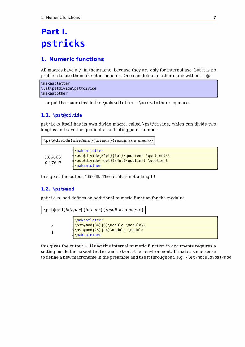
1. Numeric functions
All macros have a @ in their name, because they are only for internal use, but it is no
problem to use them like other macros. One can define another name without a @:
\makeatletter
\let\pstdivide\pst@divide
\makeatother
or put the macro inside the \makeatletter – \makeatother sequence.
1.1. \pst@divide
pstricks itself has its own divide macro, called \pst@divide, which can divide two
lengths and save the quotient as a floating point number:
\pst@divide{dividend}{divisor}{result as a macro}
5.66666
-0.17647
1\makeatletter
2\pst@divide{34pt}{6pt}\quotient \quotient\\
3\pst@divide{-6pt}{34pt}\quotient \quotient
4\makeatother
this gives the output 5.66666. The result is not a length!
1.2. \pst@mod
pstricks-add defines an additional numeric function for the modulus:
\pst@mod{integer}{integer}{result as a macro}
4
1
1\makeatletter
2\pst@mod{34}{6}\modulo \modulo\\
3\pst@mod{25}{-6}\modulo \modulo
4\makeatother
this gives the output 4. Using this internal numeric function in documents requires a
setting inside the makeatletter and makeatother environment. It makes some sense
to define a newmacroname in the preamble and use it throughout, e.g. \let\modulo\pst@mod.

1.3. \pst@max 8
1.3. \pst@max
\pst@max{integer}{integer}{result as count register}
-6
11
1\newcount\maxNo
2\makeatletter
3\pst@max{-34}{-6}\maxNo \the\maxNo\\
4\pst@max{0}{11}\maxNo \the\maxNo
5\makeatother
1.4. \pst@maxdim
\pst@maxdim{dimension}{dimension}{result as a dimension register}
1234.0pt
967.39369pt
1\newdimen\maxDim
2\makeatletter
3\pst@maxdim{34cm}{1234pt}\maxDim \the\maxDim\\
4\pst@maxdim{34cm}{123pt}\maxDim \the\maxDim
5\makeatother
1.5. \pst@mindim
\pst@mindim{dimension}{dimension}{result as dimension register}
967.39369pt
123.0pt
1\newdimen\minDim
2\makeatletter
3\pst@mindim{34cm}{1234pt}\minDim \the\minDim\\
4\pst@mindim{34cm}{123pt}\minDim \the\minDim
5\makeatother
1.6. \pst@abs
\pst@abs{integer}{result as a count register}
34
4
1\newcount\absNo
2\makeatletter
3\pst@abs{-34}\absNo \the\absNo\\
4\pst@abs{4}\absNo \the\absNo
5\makeatother
1.7. \pst@absdim
\pst@absdim{dimension}{result as a dimension register}
967.39369pt
0.00006pt
1\newdimen\absDim
2\makeatletter
3\pst@absdim{-34cm}\absDim \the\absDim\\
4\pst@absdim{4sp}\absDim \the\absDim
5\makeatother

1.8. \pst@int 9
1.8. \pst@int
\pst@int{number}{result as a truncated integer}
-34
234
1\makeatletter
2\pst@int{-34.0}\\
3\pst@int{234.123}
4\makeatother
1.9. \pstFPDiv
\pstFPDiv{result as a truncated integer}{number}{number}
-145
-0
7
1\makeatletter
2\pstFPDiv\Result{-3.405}{0.02345} \Result\\
3\pstFPDiv\Result{0.02345}{-3.405} \Result\\
4\pstFPDiv\Result{234.123}{33} \Result
5\makeatother
1.10. \psGetSlope
\psGetSlope(x1,y1)(x2,y2)\〈macro〉
0.0
2.0
-0.2
0.00615
1\psGetSlope(-2,1)(3,1)\SlopeVal \SlopeVal\\
2\psGetSlope(-2,1)(-3,-1)\SlopeVal \SlopeVal\\
3\psGetSlope(-2,0)(3,-1)\SlopeVal \SlopeVal\\
4\psGetSlope(-2111,-12)(3,1)\SlopeVal \SlopeVal

2. Dashed Lines 10
2. Dashed Lines
Tobias Nähring has implemented an enhanced feature for dashed lines. The number
of arguments is no longer limited.
dash=value1 unit value2 unit . . .
1\psset{linewidth=2.5pt,unit=0.6}
2\begin{pspicture}(-5,-4)(5,4)
3 \psgrid[subgriddiv=0,griddots=10,
gridlabels=0pt]
4 \psset{linestyle=dashed}
5 \pscurve[dash=5mm 1mm 1mm 1mm,linewidth
=0.1](-5,4)(-4,3)(-3,4)(-2,3)
6 \psline[dash=5mm 1mm 1mm 1mm 1mm 1mm 1mm
1mm 1mm 1mm](-5,0.9)(5,0.9)
7 \psccurve[linestyle=solid](0,0)(1,0)(1,1)
(0,1)
8 \psccurve[linestyle=dashed,dash=5mm 2mm
0.1 0.2,linetype=0](0,0)(-2.5,0)
(-2.5,-2.5)(0,-2.5)
9 \pscurve[dash=3mm 3mm 1mm 1mm,linecolor=
red,linewidth=2pt](5,-4)(5,2)(4.5,3.5)
(3,4)(-5,4)
10\end{pspicture}
3. "‘Handmade"’ lines :-) 11
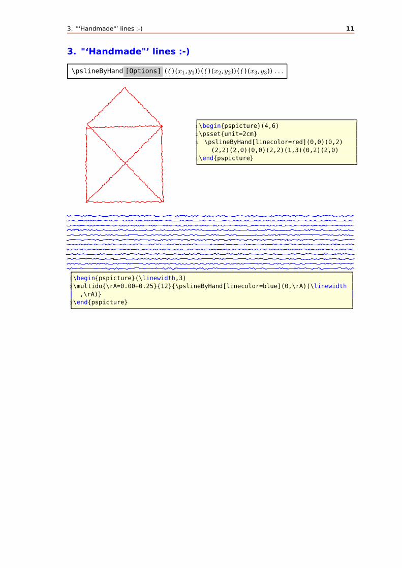
3. "‘Handmade"’ lines :-)
\pslineByHand [Options] (()(x1,y1))(()(x2,y2))(()(x3,y3)) . . .
1\begin{pspicture}(4,6)
2\psset{unit=2cm}
3 \pslineByHand[linecolor=red](0,0)(0,2)
(2,2)(2,0)(0,0)(2,2)(1,3)(0,2)(2,0)
4\end{pspicture}
1\begin{pspicture}(\linewidth,3)
2\multido{\rA=0.00+0.25}{12}{\pslineByHand[linecolor=blue](0,\rA)(\linewidth
,\rA)}
3\end{pspicture}
4. \rmultiput: a multiple \rput 12
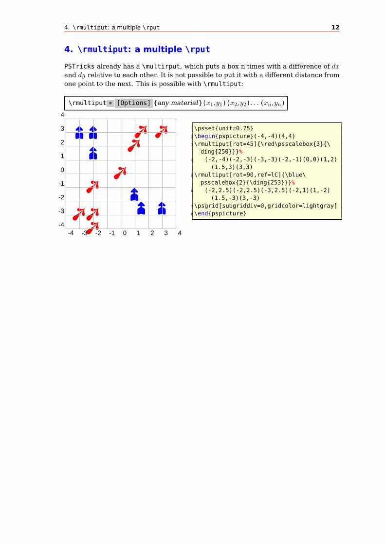
4. \rmultiput: a multiple \rput
PSTricks already has a \multirput, which puts a box n times with a difference of dxand dy relative to each other. It is not possible to put it with a different distance from
one point to the next. This is possible with \rmultiput:
\rmultiput * [Options] {any material}(x1,y1)(x2,y2). . . (xn,yn)
úúú
úú
úú úýýý
ý
ýý ý
-4 -3 -2 -1 0 1 2 3 4-4
-3
-2
-1
0
1
2
3
4
1\psset{unit=0.75}
2\begin{pspicture}(-4,-4)(4,4)
3\rmultiput[rot=45]{\red\psscalebox{3}{\
ding{250}}}%
4 (-2,-4)(-2,-3)(-3,-3)(-2,-1)(0,0)(1,2)
(1.5,3)(3,3)
5\rmultiput[rot=90,ref=lC]{\blue\
psscalebox{2}{\ding{253}}}%
6 (-2,2.5)(-2,2.5)(-3,2.5)(-2,1)(1,-2)
(1.5,-3)(3,-3)
7\psgrid[subgriddiv=0,gridcolor=lightgray]
8\end{pspicture}

5. \psrotate: Rotating objects 13
5. \psrotate: Rotating objects
\rput also has an optional argument for rotating objects, but it always depends on
the \rput coordinates. With \psrotate the rotating center can be placed anywhere.
The rotation is done with \pscustom, all optional arguments are only valid if they are
part of the \pscustom macro.
\psrotate [Options] (x, y){rot angle}{object}
1
2
3
4
−1
−2
−3
1 2 3 4 5 6 7 8
b
1\psset{unit=0.75}
2\begin{pspicture}(-0.5,-3.5)(8.5,4.5)
3 \psaxes{->}(0,0)(-0.5,-3)(8.5,4.5)
4 \psdots[linecolor=red,dotscale=1.5](2,1)
5 \psarc[linecolor=red,linewidth=0.4pt,
showpoints=true]
6 {->}(2,1){3}{0}{60}
7 \pspolygon[linecolor=green,linewidth=1pt
](2,1)(5,1.1)(6,-1)(2,-2)
8 \psrotate(2,1){60}{%
9 \pspolygon[linecolor=blue,linewidth=1pt
](2,1)(5,1.1)(6,-1)(2,-2)}
10\end{pspicture}
-1 0 10
1
2
3
4
5
-1
0
1
0
1
2
3
4
5
-10
1012345
-1 0 10
1
2
3
4
5
b
1\def\canne{% Idea by Manuel Luque
2 \psgrid[subgriddiv=0](-1,0)(1,5)
3 \pscustom[linewidth=2mm]{\psline(0,4)\
psarcn(0.3,4){0.3}{180}{360}}%
4 \pscircle*(0.6,4){0.1}\pstriangle*(0,0)
(0.2,-0.3)}
5\def\Object{}
6\begin{pspicture}(-1,-1)(3,6)
7 \canne
8 \psrotate(0.3,4){45}{\psset{linecolor=red
!50}\canne}
9 \psrotate(0.3,4){90}{\psset{linecolor=
blue!50}\canne}
10 \psrotate(0.3,4){360}{\psset{linecolor=
cyan!50}\canne}
11 \psdot[linecolor=red](0.3,4)
12\end{pspicture}

5. \psrotate: Rotating objects 14
0
1
2
3
4
−1
−2
−3
−4
−5
1 2 3 4 5 6 7 8 9 10 11 12 13 14
b
b
b
b
b
b
b
b
b
b
b
b
b
b
b
bb
b
b
b
b
b
b
b
b
b
b
b
b
b
b
b
b
b
b
b
b
b
b
b
b
b
b
b
b
b
b
b
b
b
b
b
b
b
b
b
b
b
b
b
b
b
b
b
b
b
b
bb
b
b
b
b
b
b
b
b
b
b
b
b
b
1\def\majorette{\psline[linewidth=0.5mm](0,2)% Idea by Manuel Luque
2 \pscircle[fillstyle=solid]{0.1}
3 \pscircle[fillstyle=solid](0,2){0.1}}
4\begin{pspicture}(0,-6)(15,5)
5 \psaxes[linewidth=0.5pt]{->}(0,0)(0,-5)(15,5)
6 \pstVerb{/V0 10 def /Alpha 45 def}% vitesse initiale, angle de lancement
7 \multido{\nT=0.0+0.05,\iA=0+40}{41}{%
8 \pstVerb{/nT \nT\space def}%
9 \rput(!V0 Alpha cos mul nT mul -9.81 2 div nT dup mul mul V0 Alpha sin
mul nT mul add){%
10 \psrotate(0,1){\iA}{\majorette\psdot[linecolor=red](0,1)\psdot[
linecolor=green](0,2)}}}
11 \parametricplot[linecolor=red]{0}{2}{% trajectoire du milieu
12 V0 Alpha cos mul t mul -9.81 2 div t dup mul mul V0 Alpha sin mul t mul
add 1 add}
13 \parametricplot[linecolor=green,plotpoints=360]{0}{2}{% d’une extremite
14 V0 Alpha cos mul t mul 800 t mul sin sub % x(t)
15 -9.81 2 div t dup mul mul V0 Alpha sin mul t mul add 1 add 800 t mul cos
add }%y(t)
16\end{pspicture}

6. \psComment: comments to a graphic 15
6. \psComment: comments to a graphic
\psComment * [Options] {arrows} (x0,y0)(x1,y1){Text} [line macro]
By default the macro uses the \ncline macro to draw a line from the first to the
second point. With the second additional argument one can use another macro for
the line.
Mantelstift
Kernstift
Feder
Nur für Profil
1\SpecialCoor\newpsstyle{weiss}{fillstyle=solid,fillcolor=white}
2\footnotesize\psset{unit=0.5cm,dimen=middle}
3\begin{pspicture}(-12,-4)(6,10)
4\psframe*[linecolor=black!20](-5,-3)(5,7) \psframe*[linecolor=black!40](-5,3)(5,6)
5\pscircle(-8.19,5.51){0.2}
6\psframe[fillcolor=white,fillstyle=solid](-5.8,3.6)(4.3,5.8)
7\psframe(-8.98,3.14)(-5.8,6.32)
8\multido{\rA=-4.1+1.3}{5}{\rput(\rA,-2.4){\psframe[style=weiss](1.1,6)
9 \psline(0,0)(1.1,0.5)(0,1)(1.1,1.6)(0,2.2)(1.1,2.7)(0,3.2)(1.1,3.2)}}
10\pspolygon*(-4.1,3.7)(-4.1,3)(-3,3)(-3.01,3.7)(-3.54,4.19)
11\pspolygon*(1.09,3.7)(1.1,3)(2.2,3)(2.18,3.7)(1.65,4.24)
12\pspolygon*(-2.78,3.7)(-2.8,3)(-1.7,3)(-1.71,3.7)(-2.27,4.04)
13\pspolygon*(-1.51,3.7)(-1.5,3)(-0.4,3)(-0.41,3.7)(-1.02,4.17)
14\pspolygon*(-0.21,3.7)(-0.2,3)(0.9,3)(0.89,3.7)(0.3,4.04)
15\psline(-5,3.83)(-4.15,3.86)(-3.5,4.3)(-2.85,3.81)(-2.22,4.21)(-1.6,3.86)(-0.99,4.33)
16 (-0.28,3.83)(0.35,4.19)(0.97,3.83)(1.65,4.39)(2.2,4.01)(3.57,4.89)(2.41,5.8)
17 \psline(-5,5.8)(-5.78,5.8) \psline(-5.78,5.47)(2.85,5.47)
18 \psline(-5.8,3.52)(-5,3.5) \psline(3.57,4.89)(-5.8,4.89)
19 \psComment*[ref=r]{->}(-8.14,1.19)(-4.31,3.27){Mantelstift}
20 \psComment*[ref=r]{->}(-8.17,-0.56)(-4.37,1.59){Kernstift}[\rput]
21 \psComment*[ref=r]{->}(-7.91,-2.24)(-4.44,-0.23){Feder}[\rput]
22 \psComment[npos=-0.1]{->}(-3.48,8.72)(-1.33,5.46){Nur f\"ur Profil}
23\end{pspicture}

7. \psChart: a pie chart 16
7. \psChart: a pie chart
\psChart [Options] {comma separated value list}{comma separated value list}{radius}
The special optional arguments for the \psChart macro are as follows:
name description default
chartSep distance from the pie chart center to an outraged pie piece 10pt
chartColor gray or colored pie (values are: gray or color) gray
userColor a comma separated list of user defined colors for the pie {}
The first mandatory argument is the list of the values and may not be empty. The
second one is a list of outraged pieces, numbered consecutively from 1 to up the total
number of values. The list of user defined colors must be enclosed in braces!
The macro \psChart defines for every value three nodes at the half angle and in
distances from 0.75, 1, and 1.25 times of the radius from the origin. The nodes are
named as psChartI?, psChart?, and psChartO?, where ? is the number of the pie.
The letter I leads to the inner node and the letter O to the outer node. The distance
can be changed with the optional arguments chartNodeI and chartNodeO in the usual
way with \psset{chartNodeI=...,chartNodeO=...}.
The other one is the node on the circle line. The origin is by default (0,0). Moving
the pie to another position can be done as usual with the \rput-macro. The used
colors are named internally as chartFillColor? and can be used by the user for
coloring lines or text.
b
b
bb
b
b
bb
b
bb
b
b
b
b
bb
b
1\begin{pspicture}(-3,-3)(3,3)
2\psChart{ 23, 29, 3, 26, 28, 14 }{}{2}
3\multido{\iA=1+1}{6}{%
4 \psdot(psChart\iA)\psdot(psChartI\iA)\
psdot(psChartO\iA)%
5 \psline[linestyle=dashed,linecolor=white
](psChart\iA)
6 \psline[linestyle=dashed](psChart\iA)(
psChartO\iA)}
7\end{pspicture}

7. \psChart: a pie chart 17
pie no 1
pie no 2
1\begin{pspicture}(-3,-3)(3,3)
2\psChart[chartColor=color]{ 45, 90 }{ 1
}{2}
3\ncline[linecolor=-chartFillColor1,
4 nodesepB=-20pt]{psChartO1}{psChart1}
5\rput[l](psChartO1){%
6 \textcolor{chartFillColor1}{pie no 1}}
7\ncline[linecolor=-chartFillColor2,
8 nodesepB=-20pt]{psChartO2}{psChart2}
9\rput[lt](psChartO2){%
10 \textcolor{chartFillColor2}{pie no 2}}
11\end{pspicture}
pie no 1
pie no 2
pie no 3
pie no 4
pie no 5
pie no 6
pie no 7
pie no 8
pie no 9
1\psframebox[fillcolor=black!20,
2 fillstyle=solid]{%
3\begin{pspicture}(-3.5,-3.5)
(4.25,3.5)
4\psChart[chartColor=color]%
5 {23, 29, 3, 26, 28, 14, 17, 4,
9}{}{2}
6\multido{\iA=1+1}{9}{%
7 \ncline[linecolor=-chartFillColor
\iA,
8 nodesepB=-10pt]{psChartO\iA}{
psChart\iA}
9 \rput[l](psChartO\iA){%
10 \textcolor{chartFillColor\iA}{
pie no \iA}}}
11\end{pspicture}}
1\begin{pspicture}(-3,-3)(3,3)
2\psChart[userColor={red!30,green!30,
3 blue!40,gray,magenta!60,cyan}]%
4 { 23, 29, 3, 26, 28, 14 }{1,4}{2}
5\end{pspicture}

7. \psChart: a pie chart 18
1
2
3
4
5
6
1\begin{pspicture}(-3,-2.5)(3,2.5)
2\psChart{ 23, 29, 3, 26, 28, 14 }{}{2}
3\multido{\iA=1+1}{6}{\rput*(psChartI\iA){\
iA}}
4\end{pspicture}
1000 (34.5%)
500 (17.2%)
600 (20.7%)
450 (15.5%)
150 (5.2%)
200 (6.9%)
Taxes
Rent
Bills
Car
Gas
Food
1 \psset{unit=1.5}
2 \begin{pspicture}(-3,-3)(3,3)
3 \psChart[userColor={red!30,green!30,blue!40,gray,cyan!50,
4 magenta!60,cyan},chartSep=30pt,shadow=true,shadowsize=5pt
]{34.5,17.2,20.7,15.5,5.2,6.9}{6}{2}
5 \psset{nodesepA=5pt,nodesepB=-10pt}
6 \ncline{psChartO1}{psChart1}\nput{0}{psChartO1}{1000 (34.5\%)}
7 \ncline{psChartO2}{psChart2}\nput{150}{psChartO2}{500 (17.2\%)}
8 \ncline{psChartO3}{psChart3}\nput{-90}{psChartO3}{600 (20.7\%)}
9 \ncline{psChartO4}{psChart4}\nput{0}{psChartO4}{450 (15.5\%)}
10 \ncline{psChartO5}{psChart5}\nput{0}{psChartO5}{150 (5.2\%)}
11 \ncline{psChartO6}{psChart6}\nput{0}{psChartO6}{200 (6.9\%)}
12 \bfseries%
13 \rput(psChartI1){Taxes}\rput(psChartI2){Rent}\rput(psChartI3){Bills}
14 \rput(psChartI4){Car}\rput(psChartI5){Gas}\rput(psChartI6){Food}
15 \end{pspicture}

8. \psHomothetie: central dilatation 19
8. \psHomothetie: central dilatation
\psHomothetie [Options] (center){factor}{object}
-5 -4 -3 -2 -1 0 1 2 3 4-4
-3
-2
-1
0
1
2
3
4
5
6
7
8
b
1\begin{pspicture}[showgrid
=true](-5,-4)(4,8)
2\psBill% needs package pst
-fun
3\psHomothetie[linecolor=
blue](4,-3){2}{\psBill}
4\psdots[dotsize=3pt,
linecolor=red](4,-3)
5\psplot[linestyle=dashed,
linecolor=red]{-5}{4}%
6 [ /m -3 -0.85 sub 4 0.6
sub div def ]
7 { m x mul m 4 mul sub 3
sub }%
8\psHomothetie[linecolor=
green](4,-3){-0.2}{\
psBill}
9\end{pspicture}

9. \psbrace 20
9. \psbrace
9.1. Syntax
\psbrace * [Options] (A)(B){text}
0 1 2 3 40
1
2
3
4
Text I
Text
II
III
1\begin{pspicture}(4,4)
2\psgrid[subgriddiv=0,griddots=10]
3\pnode(0,0){A}
4\pnode(4,4){B}
5\psbrace[linecolor=red,ref=lC](A)(B){Text I}
6\psbrace*[linecolor=blue,ref=lC](3,4)(0,1){Text II
}
7\psbrace[fillcolor=white](3,0)(3,4){III}
8\end{pspicture}
The option \specialCoor is enabled, so that all types of coordinates are possible,
(nodename), (x, y), (nodeA|nodeB), . . . The star version fills the inner of the brace with
the current linecolor. With the fillcolor white or any other background color the brace
can be "‘unfilled"’.
9.2. Options
Additional to all other available options from pstricks or the other related packages,
there are two new option, named braceWidth and bracePos. All important ones are
shown in the following graphics and table.
0 1 2 3 4 5 6 7 8 9 100
1
2
3
4
5
Label
braceWidth
braceWidthInner
braceWidthOuter
nodesepB
A
bracePos
b A bB

9.2. Options 21
A positive value for nodesepA and nodesepB shifts the label to the upper right and
a negative value to the lower left. This does not depends on the value for the rotating
of the label!
name meaning
braceWidth default is \pslinewidth
braceWidthInner default is 10\pslinewidth
braceWidthOuter default is 10\pslinewidth
bracePos relative position (default is 0.5)nodesepA x-separation (default is 0pt)nodesepB y-separation (default is 0pt)rot additional rotating for the text (default is 0)ref reference point for the text (default is c)
fillcolor default is black
By default the text is written perpendicular to the brace line and can be changed
with the pstricks option rot=. . . The text parameter can take any object and may
also be empty. The reference point can be any value of the combination of l (left) or
r (right) and b (bottom) or B (Baseline) or C (center) or t (top), where the default is c,
the center of the object.
Text TextText
Text
Text
1\begin{pspicture}(8,2.5)
2\psbrace(0,0)(0,2){\fbox{Text}}%
3\psbrace[nodesepA=10pt](2,0)(2,2)
{\fbox{Text}}
4\psbrace[ref=lC](4,0)(4,2){\fbox{
Text}}
5\psbrace[ref=lt,rot=90,nodesepB
=-15pt](6,0)(6,2){\fbox{Text}}
6\psbrace[ref=lt,rot=90,nodesepA=-5
pt,nodesepB=15pt](8,2)(8,0){\
fbox{Text}}
7\end{pspicture}
∞∫
1
1x2 dx = 1 ∞ ∫ 1
1 x2dx
=1
∞∫
1
1x2 dx = 1
∞ ∫ 1
1 x2dx
=1
∞∫1
1x2dx
=1
1\def\someMath{$\int\limits_1^{\
infty}\frac{1}{x^2}\,dx=1$}
2\begin{pspicture}(8,2.5)
3\psbrace[ref=lC](0,0)(0,2){\
someMath}%
4\psbrace[rot=90](2,0)(2,2){\
someMath}
5\psbrace[ref=lC](4,0)(4,2){\
someMath}
6\psbrace[ref=lt,rot=90,nodesepB
=-30pt](6,0)(6,2){\someMath}
7\psbrace[ref=lt,rot=90,nodesepB=30
pt](8,2)(8,0){\someMath}
8\end{pspicture}
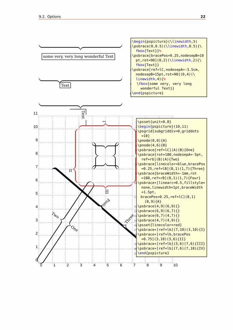
9.2. Options 22
Text
Text
some very, very long wonderful Text
1\begin{pspicture}(\linewidth,5)
2\psbrace(0,0.5)(\linewidth,0.5){\
fbox{Text}}%
3\psbrace[bracePos=0.25,nodesepB=10
pt,rot=90](0,2)(\linewidth,2){\
fbox{Text}}
4\psbrace[ref=lC,nodesepA=-3.5cm,
nodesepB=15pt,rot=90](0,4)(\
linewidth,4){%
5 \fbox{some very, very long
wonderful Text}}
6\end{pspicture}
0 1 2 3 4 5 6 7 8 9 100
1
2
3
4
5
6
7
8
9
10
11
One
Two
Three
Four
A
I
II
III
IV
1\psset{unit=0.8}
2\begin{pspicture}(10,11)
3\psgrid[subgriddiv=0,griddots
=10]
4\pnode(0,0){A}
5\pnode(4,6){B}
6\psbrace[ref=lC](A)(B){One}
7\psbrace[rot=180,nodesepA=-5pt,
ref=rb](B)(A){Two}
8\psbrace[linecolor=blue,bracePos
=0.25,ref=lB](8,1)(1,7){Three}
9\psbrace[braceWidth=-1mm,rot
=180,ref=rB](8,1)(1,7){Four}
10\psbrace*[linearc=0.5,fillstyle=
none,linewidth=1pt,braceWidth
=1.5pt,
11 bracePos=0.25,ref=lC](8,1)
(8,9){A}
12\psbrace(4,9)(6,9){}
13\psbrace(6,9)(6,7){}
14\psbrace(6,7)(4,7){}
15\psbrace(4,7)(4,9){}
16\psset{linecolor=red}
17\psbrace*[ref=lb](7,10)(3,10){I}
18\psbrace*[ref=lb,bracePos
=0.75](3,10)(3,6){II}
19\psbrace*[ref=lb](3,6)(7,6){III}
20\psbrace*[ref=lb](7,6)(7,10){IV}
21\end{pspicture}

9.2. Options 23
1. . .
10
. . .
0
ntim
es
ntim
es
1\[
2\begin{pmatrix}
3 \Rnode[vref=2ex]{A}{~1} \\
4 & \ddots \\
5 && \Rnode[href=2]{B}{1} \\
6 &&& \Rnode[vref=2ex]{C}{0} \\
7 &&&& \ddots \\
8 &&&&& \Rnode[href=2]{D}{0}~ \\
9\end{pmatrix}
10\]
11\psbrace[rot=-90,nodesepB=-0.5,nodesepA=-0.2](B
)(A){\small n times}
12\psbrace[rot=-90,nodesepB=-0.5,nodesepA=-0.2](D
)(C){\small n times}
It is also possible to put a vertical brace around a default paragraph. This works by
setting two invisible nodes at the beginning and the end of the paragraph. Indentation
is possible with a minipage.
Some nonsense text, which is nothing more than nonsense. Some nonsense text,
which is nothing more than nonsense.
Some nonsense text, which is nothing more than nonsense. Some nonsense text,
which is nothing more than nonsense. Some nonsense text, which is nothing more
than nonsense. Some nonsense text, which is nothing more than nonsense. Some
nonsense text, which is nothing more than nonsense. Some nonsense text, which
is nothing more than nonsense. Some nonsense text, which is nothing more than
nonsense. Some nonsense text, which is nothing more than nonsense.
Some nonsense text, which is nothing more than nonsense. Some nonsense text,
which is nothing more than nonsense.
Some nonsense text, which is nothing more than nonsense. Some nonsense text,
which is nothing more than nonsense. Some nonsense text, which is nothing more
than nonsense. Some nonsense text, which is nothing more than nonsense. Some
nonsense text, which is nothing more than nonsense. Some nonsense text, which
is nothing more than nonsense. Some nonsense text, which is nothing more than
nonsense. Some nonsense text, which is nothing more than nonsense.
1 Some nonsense text, which is nothing more than nonsense.
2 Some nonsense text, which is nothing more than nonsense.
3
4 \noindent\rnode{A}{}
5
6 \vspace*{-1ex}
7 Some nonsense text, which is nothing more than nonsense.
8 Some nonsense text, which is nothing more than nonsense.
9 Some nonsense text, which is nothing more than nonsense.
10 Some nonsense text, which is nothing more than nonsense.
11 Some nonsense text, which is nothing more than nonsense.
12 Some nonsense text, which is nothing more than nonsense.
13 Some nonsense text, which is nothing more than nonsense.
14 Some nonsense text, which is nothing more than nonsense.
15

9.2. Options 24
16 \vspace*{-2ex}\noindent\rnode{B}{}\psbrace[linecolor=red](A)(B){}
17
18 Some nonsense text, which is nothing more than nonsense.
19 Some nonsense text, which is nothing more than nonsense.
20
21 \medskip\hfill\begin{minipage}{0.95\linewidth}
22 \noindent\rnode{A}{}
23
24 \vspace*{-1ex}
25 Some nonsense text, which is nothing more than nonsense.
26 Some nonsense text, which is nothing more than nonsense.
27 Some nonsense text, which is nothing more than nonsense.
28 Some nonsense text, which is nothing more than nonsense.
29 Some nonsense text, which is nothing more than nonsense.
30 Some nonsense text, which is nothing more than nonsense.
31 Some nonsense text, which is nothing more than nonsense.
32 Some nonsense text, which is nothing more than nonsense.
33
34 \vspace*{-2ex}\noindent\rnode{B}{}\psbrace[linecolor=red](A)(B){}
35 \end{minipage}

10. Random dots 25
10. Random dots
The syntax of the new macro \psRandom is:
\psRandom [Options] {}
\psRandom [Options] (xMin, yMin) (xMax, yMax) {clip path}
If there is no area for the dots defined, then (0,0)(1,1) in the current scale setting
is used for placing the dots. If there is only one (xMax, yMax) defined, then (0,0) is
used for the other point. This area should be greater than the clipping path to be sure
that the dots are placed over the full area. The clipping path can be everything. If no
clipping path is given, then the frame (0,0)(1,1) in user coordinates is used. The
new options are:
name default
randomPoints 1000 number of random dots
color false random color
b
b
b
b
b
b
b
b
b
b
b
b
b
b
b
b
b
b
b
b
b
b
b
b
b
b
b
b
b
b
b
b
b
b
b
b
b
b
b
b
b
b
b
b
b
b
b
b
b
b
b
b
b
b
b
b
b
b
b
b
b
b
b
b
b
b
b
b
b
b
b
b
b
b
b
b
b
b
b
b
b
b
b
b
b
b
b
b
b
b
b
b
b
b
b
b
b
b
b
b
bb
b
b
b
b
b
b
b
b
b
b
b
b
b
b
b
b
b
b
b
b
b
b
b
b
b
b
b
b
b
b
b
b
b
b
bb
b
b
b
b
b
b
b
b
b
b
b
b
b
b
b
b
b
b
bb
b
b
b
b
b
b
b
b
b
b
b
b
b
b
b
b
b
b
b
b
b
b
b
b
b
b
b
b
b
b
b
b
b
b
b
b
b
b
b
b
b
b
b
b
b
b
b
b b
b
b
b
b
b
b
b
b
b
b
b
b
b
b
b
b
b
b
b
b
b
b
b
b
b
b
b
b
b
b
b
b
b
b
b
b
b
b
b
b
b
b
b
b
b
b
b
b
b
b
b
b
b
b
b
b
b
b
b
b
bb
b
b
b
b
b
b
b
b
b
b
b
b
b
b
b
b
b
b
b
b
b
b
b
b
b
b
b
b
b
b
b
b
b
b
b
b
b
b
b
b
b
b
b
bb
b
b
b
b
b
b
b
b
b
b
b
b
b
b
b
b
b
b
b
b
b
b
b
b
b
b
bb
b
b
b
b
b
b
b
b
b
b
b
b
b
b
b
b
bb
b
b
b
b
b
b
b
b
b
b
b
b
b
b
b
b
b
b
b
b
b
b
b
b
b
b
b
b
b
b
b
b
b
b
b
b
b
b
b
b
b
b
b
b
b
b
b
b
b
bb
b
b
b
b
b
b
b
b
b
b
b
bb
b
b
b
b
b
b
b
b
b
b
b
b
b
b
b
b
b
b
b
b
b
b
b
b
b
b
b
b
b
b
b
b
b
b
b
b
b
b
b
b
b
b
b
b
b
b
b
b
b
b
bb
bb
b
b
b
b
b
b
b
b
b
b
b
b
b
b
b
b
b
b
b
b
b
b
b
b
b
b
b
b
b
b
bb
b
b
b
b
b
b
b
b
b
b
b
b
b
b
b
b
b
bb
b
b
b
b
b
b
b
b
b
b
b
b
b
b
b
b
b
b
b
b
b
b
b
b
b
b
b
b
b
b
b
b
b
b
b
b
b
b
b
b
b
b
b
b
b
b
b
b
b
b
b
b
b
b
b
b
b
b
b
b
b
b
b
b
b
b
b
b
b
b
b
b
b
b
b
b
b
b
b
b
b
b
b
b
b
b
b
b
b
b
b
b
b
b
b
b
b
b
b
b
b
b
b
b
b
b
b
b
b
b
b
b
b
b
b
b
b
b
b
b
b
b
b
b
b
b
b
b
b
b
b
b
b
b
b
b
b
b
b
b
b
b
b
b
b
b
b
b
b
b
b
b
bb
b
bb
b
b
b
b
b
b
b
b
b
bb
b
b
b
b
b
b
b
b
b
b
b
b
b
b
b
b
b
b
b
b
b
b
b
b
b
b
bb
b
b
b
b
b
b
b
b
b
b
b
b
b
b
b
b
b
b
b
b
b
b
b
b
b
b
b
b
b
b
b
b
b
b
b
b
b
b
b
b
b
b
b
b
b
b
b
b
b
b
b
b
b
b
b
b
b
b
b
b
b
b
b
b
b
b
b
b
b
b
b
b
b
b
b
b
b
b
b
b
b
b b
b
b
b
b
b
b
b
bb
b
b
b
b
bb
b
b
b
b
b
b
b
b
b
b
b
b
b
b
b
b
b
b
b
b
b
b
b
b
b
b
b
b
b
b
b
b
b
b
b
bb
b
b
b
b
b
b
b
b
b
b
b
b
b
b
b
b
b
b
b
b
b
b
b
b
b
b
b
b
b
b
b
b
b
b
b
b
b
b
b
b
b
b
b
b
b
b
b
b
b
b
b
bb
b
b
b
b
b
b
b
b
b
b
b
b
b
b
b
b
b
b
b
b
b
b
b
b
b
b
b
b
b
b
b
b
b
b
b
b
b
b
b
b
b
b
b
b
b
b
b
b
b
b
b
b
b
b
b
b
b
b
b
b
b
b
b
b
b
b
b
b
b
b
b
b
b
b
b
b
b
b
b
b
b
b
b
b
b
b
b
b
b
b
b
b
b
b
b
b
b
b
b
b
b
b
b
b
b
b
b
bb
b
b
b
b
b
b
b
b
b
b
b
b
b
b b
b
b
b
b
b
b
b
b
b
b
b
b
b
b
b
b
b
b
b
b
b
b
b
b
b
b
b
b
b
bb
b
b
b
b
b
b
b
bb
b
b
b
b
b
b
b
b
b
b
b
b
b
b
b
b
b
b
b
b
b
b
b
b
b
b
b
b
b
bb
b
b
b
b
b
bb
b
b
b
b
b
b
b
b
b
b
b b
b
b
b
b
b
b
b
b
b
b b
b
bb
b
b
b
b
b
b
bb
b
b
b
b
b
b
b
b
b
b
b
b
b
b
b
b
b
b b
b
b
b
bb
b
b
b
b
b
bb
b
b
b
b
b
b
b
b
b
b
b
b
b
b
bb
b
b
b
b
b
b
b
b
b
b
b
b
b
b
b
b
b
b
b
b
b
b
b
b
b
b
b
b
b
b
b
b
b
b
b
b
b
b
b
b
b
b
b
b
b
b
bb
b
b
b
b
b
b
b
b
b
b
b
b
b
b
b
b
b
b
b
b
b
b
b
b
b
b
b
bb
b
b
b
b
b b
b
b
b
b
b
b
b
b
b
b
b
b
b
b
b
b
b
b
b
b
b
b
b
b
b
b
bb
b
b
b
b
b
b
b
b
b
b
b
b
b
b
b
b
b
b
b
b
b
b
b
bb
b
b
b
bb
b
b
b
b
b
b
b
b
b
b
b
b
b
b b
b
b
b
b
b
b
b
b
b
b
b
b
b
b
b
b
b
b
b
b
b
b
bb
b
b
b
b
b
b
b
bb
b
b
b
bb
b
b
b
b
b
b
b
b
b
b
b
b
b
b
b
b
b
b
b
b
b
b
bb
b
b
b
bb
b
b
b
b
b
b
b
bb
b
b
b
bb
b
b
b
b
b
b
b
bb
bb
b
b
b
b
b
b
b
bb
b
b
b
b
b
b
b
b
b
b
bb
bb
b
b
b
b
b
b
b
b
b
b
b
b
b
b
b
b
b
b
b
b
b
b
b
b
b
b
bb
b
b
bb
b
b
b
b
b
b
b
b
b
b
b
b
b
b
b
b
b
b
b
b
b
b
b
b
b
b
b
b
b
b
b
b
b
b
b
b
b
b
b
b
b
b
b
b
b
b
b
b
b
b
bb
b
b
b
b
b
b
b
b
b
b
b
b
b
b
b
bb
b
b
b b
b
b
b b
b
b
b
b
b
b
b
b
b
b
b
b
b
b
b
b
b
b
b
b
bb
b
b
b
b
b
b
b
b
b
b
b
b
b
b
b
b
b
b
b
b
b
b
b
bb
b
b
b
b
b
b
b
b
b
b
b
b
b
b
b
b
b
b
b
b
b
b
b
b
b
b
b
b
b
b
b
b
b
bb
b
b
b
b
b
b
b
b
b
b
b
bb
b
b
b
b
b
b
b
b
b
bb
b
b
b
b
b
b
b
b
b
b
b
b
b
b
b
b
b
b
b
b
b b
b
b
b
b
b
b
b
b
b
bb
b
b
bb
b
b
b
b
b
b
b
b
b
b
b
b
b
b
b
b
b
b
b
bb
b
b
b
b
b
b
b
b
b
b
b
b
b
b
b
b
b
b
b
b
bb
b
b b
b
b b
b
b
b
b
b
bb
b
b
b
b b
b
b
b
b
b
b
b
b
b
b
b
b
b
b
b
b
b
b
b
b
b
b
b
b
b
b
b
b
b
b
b
b
b
b
b
b
b
b
b
b
b
b
b
b
b
b
b
b
b
b
b
b
b
b
b
b
b
b
b
b
b
b
b
b
b
b
b
b
b
b
b
b
b b
b
b
b
b
b
b
b
b
b
b
b
b
b
b
b
b
b
b
b
b
bb
b
b
b
b
b
b
b
b
b
b
b
b
b
b
b
b
b
b
b
b
b
b
b
b
b
b
bb
b
b
b
b
b
b
b
b
b
b
b
bb
b
b
b
b
b
b
b
b
b
b
b
b
b
b
b
b
b
b
b
b
b
b
b
b
b
b
b
b
b
b
b
b
b
b
bb
b
b
b
b
b
b
b
b
b
b
b
b
b
b
b
b
b
b
b
b
b
b
b
b
b
b
b
b
b b
b
bb
b
b
b
b
b
b
b
b
b
b
b
b
b
b
b
b
b
b
b
b
b
b
b
b
b
b
b
b
b
bb
b
b
b
b
b
b
b
b
bb
b
b
b
b
b
b
bb
b
b
b
b
b
b
b
b
b
b
b
b
b
b
b b
b
b
b
b
b
b
b
b
b
b
b
b
b
b
b
b
b
b
b
b
b
b
b
bb
b
b
b
b
b
b
b
b b
b
b
bb
b
b
bb
b
b
b
b
b
b
b
b
b
b
bb
b
bb
b
b
b
b
b
b
b
b
b
b
b
b
b
b
b
bb
b
b
b
bb
b
b
b
b
b
b
b
b
b
b
b
b
b
b
b
b
b
b
b
b
b
b
b b
b
b
b
b
b
b
b
b
b
bb
b
b
b
b
b
b
b
b
b
b
b
b
b
b
b
b
b
b
b
b
b
b
b
b
b
b
b
bb
b
b
b
b
b
b
b
bb
b
b
b
b
b
bb
b
b
b
b
b
b
b
bb
b
b
b
b
b
b
b
b
b
b
b
b
b
b
b
b
b
b
b
b
b
b
b
b
b
b
b
b
b
b
b
b
b
b
b
b
b
b
b
b
b
b
b
b
b
b
b
b
b
b
b
b
b
b
b
b
b
b
b
b
b
b
b
b
b
b
b
b
b
bb
b
b
b
b
b
b
b
b
b
b
b
b
b
b
b
b
b
b
b
b
b
b
b
b
b
b
b
b
b
b
b
b
b
b
b
b
b
b
b
b
b
b
b
b
b
b
b
b
b
b
b
b
b
b
b
b
b
b
b
b
b
b
bb
b
b
b
bb
b
b
b
b
b
b
b
b
b
b
b
b
b
b
b
b
b
b
b
b
b
bb
b
b
b
b
b
b
b
b
b
b
b
b
b
b
b
bb
b
b
b
b
b
b
b
b
b
b
b
b
b
b
b
b
b
b
bbb
b
b
b
bb
b
bb
bbb
b
b
b
b
b
b
b
b
b
b
b
b
b
b
b
b
b
b
b
b
b
bb
b
b
b
b
b
b
b
b
b
b
b
b
b
b
b
b
bb
b
b
b
b
b
b
b
b
b
b
b
b
b
bb
b
bb
b
b
b
b
b b
b
b
b
b
b
b
b
b
b
b
b
b
b
b
b
b
b
b
b
b
b
b
b
b
b
b
b
b
b
b
b
b
b
b
b
b
b
b
b
b
b
b
b
b
b
b
bb
b
b
b
b
b
b
b
b
b
b
b
b
b
b
b
b
b
b
b
b
b
b
b
b
b
b
b
b
b
b
b
b
b
b b
b
b
b
b
b
b
b
b
b
b
b
b
b
b
b
b
b
b
bb
b
b
b
b
b
b
b
b
b b
b
b
b
bb
b
b
b
b
b
b
b
b
bb
b
b
b
b
b
b
b
b
b
b
b
bb
b
b
b
b
b
b
b
b
b
b
b
b
b
b
b
b
b
b
bb
b
b
b
b
b
b
b
b
b
b
b
bb
b
b
b
b
b
b
b
b
b
b b
b
b
b
b
b
b
b
b
b
b
b
b
b
b
b
b
b
b
b
b
b
b
b
b
b
b
b b
b
b
b
b
b
bb b
b
b
b
b
b
b
b
b
b b
b
b
b
b
b
b
b
b
b
b
b
b
b
b
b
b
b
b
bb
b
b
b
b
b
b
b
b
b
b
b
b
b
b
b
bb
b
b
b
b
b
b
bb
b
b
b
b
b
b
b
b
b
bb
b
b
b
b
bb
b
b
b
b
b
b
b
b
b
b
b
b
b
b
b
b
b
b
b
b
b
b
b
b
b
b
b
b
b
b
b
bb
b
b
b
b
b
b
bb
b
b
b
b
b
b
b
b
b
b
b
b
bb
b
b
b
b
b
b
b
b
b
b
b
b
b
b
b
b
b
b
b
b
bb
b
b
b
b
b
b
b
b
b
b
b
b
b
b
b
b
b
b
b
b
b
b
b
b b
b
b
b
b
b
bb
b
b
b
b
b
b
b
b
b
b
b
b
b
b
b
b
bb
b
b
b
b
b
bbb
b
b
b
b
bb
b
bb
b
b
b
b
b
b
b
b
bb
bb
b
b
b
b
b
b
b
b
b
b
b
b
b
b
b
b
b
b
b
b
b
b
b
b
b
b
b
b
b
b
b
b
b
b
b
b
b
b
bb
b
b
bb
b
b
b b
bb
b
b
b
b
bb
b
b
b
b
b
b
b
b
b
b
b b
b
b
b
b
b
b
b
b
b
b
b
b
b
b
b
b
b
b
b
b
b
b
b
b b
b
b
b
b
b
b
bb
b
b
b
b
b
b
b
b
b
b
b
b
b
b
b
b
bb
b
b
b
bb
b
b
b b
b
b
b
b
b
b
b
b
b
b
b
b
b
b
b
b
b
b
b
b
b
b
b
b
b
b
b
b
b
b
b
b
b
b
b
b
b
b
b
b
b
bb
b
b
b
b
b
b
b
b
b
b
b
b
b
b
b
b
b
b
b
b
b
b
b
b
b
b
b
b
b
b
b
b
b
b
b
b
b
b
b
b
b
b
b
b
b
b
b
b
b
b
b
b
b
b
b
b
b
b
b
b
b
b
b
b
b
b
b
b
b
b
b
b
b
b
b
b
b
b
b
b
b
bb
b
b
b
b
b
b
b
b
b
b
b
b
b
b
b
b
b
b
b
b
b
b
b
b
b
b
b
b
b
b
b
b
b
b
b
b
b
b
b
b
b
b
b
b
b
b
b
b
b
b
b
b
b
b
b
b
b
b
b
b
b
b
b
b
b
b
b
b
b
b
b
b
bb
b
b
b
b
b
b
b
b
b
b
b
b
b
b
b
b
b b
b
b
b
b
b
b
b
b
b
b
b
b
b
b
b
bb
b
b
b
b
b
b
b
b
b
b
b
b
b
bb
b
b
b
b
b
b
b
b
b
bb
b
b
b
b
b
b
b
b
b
b
b
b
b
b
b
b
b
b
b
b
b
b
b
b
b
b
b
b
b
b
b
b
b
b
b
b
b
b
b
b
b
b
b
b
b
b
b
b
b
b
b
b
b
b
b
b
b
b
b
b
b
b
b
b
b
b
b
b
b
b b
b
b
b
b
b
b
b
b
b
b
b
b
b
b
b
b
b
b
b
b
b
b
b
b
b
b
bb
b
b
b
b
b
b
b
b
b
b
b
b
b
b
b
b b
b
b
b
b
b
b
b
b
b
b
b
b
b
b
b
b
b
b
b
b
b
b
b
b
b
b
b
b
b
b
b
b
b
b
b
b
b
b
b
b
b
b
b
b
b
b
b
b
b
b
b
b
b
b
b
b
b
b
b
b
b
b
b
b
bb
b
b
b
b
b
b
b
b
b
b
b
b
b
b
b
b
b
b
b
b
b
b
bb
b
b
b
b
b
b
b
b
b
b
b
b
b
b
b
b
bb
b
b
b
b
b
b
b
b
b
b
b
b
b
b
b
b
b
b
b
b
b
b
b
b
b
b
b
b
b
b
b
b
b
b
b
b
b
b
b
b
b
b
b
b
b
b
b
b
b
b
b
b
b
b
b
b
b b
b
b
b
b
b
b
b
b
b
bb
b
b
b
b
b
b
b
b
b
b
b
b
b
b
b
b
b
b
b
b
b
b
b
b
b
b
b
b
b
b
b
b
b
b
b
b
b
b
b
b
b
b
b
b
b
b
b
bb
b
b
b
b
b
b
b
b
b
b
bb
b
b
b
b
b
b
b
b
b
b
b
bb
b
b
b
b b
b
b
b
b
b
b
b
b
b
b
b
b
b
b
b
b
b
b b
b
b
b
b b
b
b
b
b
b
b
b
b
b
b
b
b
bb
b
b
b b
b
b
bb
b
b
b
b
b
b
b
b
b
b
b
b
b
b
b
b
b
b
b
bb
b
b
b
b
b
b
b
b
b
b
b
b
b
b
b
b
b
b
b
b
b
b
b
b
b
b
b
b
b
b
b
b
b
b
b
b
b
b
b
b
b
b
b
b
b
b
b
b
b
b
b
b
b
b
b
b
b
b
b
b
b
b
b
b
b
b
b
b
b
b
bb
b
b
b
b
b
b
b
b
b
b
b
b
b
b
b
b
b
b
b
b
b
bb
b
b
b
b
b
b
b
b
b
b
b
b
b
b
b
b
b
b
b
b
b
b
b
b
b
b
b
b
b
b
b
b
b
b
b
b
b
b
b
b
b
b
b b
b
b
b
b
b
b
b
b
b
b
b
b
b
b
b
b
b
b
b
b
b
b
b
b
b
b
b
b
b
b
b
b
b
b
b
b
b
b
b
b
b
b
b
b
b
b
b
b
b
b
b
b
b
b
b
b
b
b
b
b
b
b
b
b
b
b
b
b
b
b
b
b
b
b
b
bb
b
b
b
b
b
b
b
b
b
b
b
b
b
b
b
b
b
b
b
b
b
b
b
b
b
b
b
b
b
b
b
b
b
b
b
b
b
b
b
b
b
b
b
b
b
b
b
b
b
b
b
b
b
b
b
b
b
b
b
bb
b
b
b
b
b
b
b
b
b
b
b
b
b
b
b
b
b
b
b
b
b
b
b
b
b
b
b
b
b
b
b
b
b
b
b
b
b
b
b
b
b
b
b
b
b
b
b
b
b
b
b
b
b
b
b
b
b
b
b
b
b
b
b
b
b
b
b
b
b
b
b
b
b
b
b
b
b
b
bb
b
b
b
b
b
bb
b
b
b
b
b
b
b
b
b
b
b
b
b
b
b
b
b
b
b
bb
b
bb
b
b
bb
b
b
b
b
bb
bbb
b
b
b
b
b
b
b
b
b
b
b
b
b
b
b
b
b
b b
b
b
b
b
b
b
bb
b
b
b
b
b
b
b
b
b
b
b
b
b
b
b
bb
b
b
b
b
b
b
b
b
b
b
b
b
bb
bb
b
b
b
b
b
b
b
b
b
b
b
b
b
b
b
b
b
b
b
b
b
b
b
b
bb
b
b
b
b
b
b
b
b
b
b
b
b
b
b
b
b
b
b
b
b
b
b
bb
bb
b
b
b
b
b
b
b
b
b
b
b
b
b
b
b
b
b
b
b
bb
b
b
b
b
b
b
b
b
b
b
b
b
b
bb
b
b
b
b
b
b
b
b
b
b
b
b
b
b
b
b
b
bb
b
b
b
b
b
b
bb
b
b
b
b
b
b
b
b
bb
b
b
b
b
b
b
b
b
b
b
b
b b
b
b
b
b
b
b
b
b
b
b
b
b
b
b
bb
b
b
b
b
b
b
b
b
b
b
b
b
b
b
b
b
b
b b
b
b
b
b
b
b
b
b
b
b
b
b
b
b
b
b
b
b
b
b
bb
b
b
b
b
b
b
b
b
b
b
b
b
b
b
b
b
b
b
b
b
b
b
b
b
b
b
b
b
b
b
b
b
b
b
b
b
b
b
b
b
b
b b
b
b
b
b
b
b
b
b
b
b
b
b
b
b
b
b
b
b
b
b
b
b
b
b
b
bb
b
b
b
b
b
b
b
b
b
b
b
b
b
b
b
b
b
b
b
b
b
bb
b
b
b
b
b
b
b
b
b
b
b
b
b
b
b
b
b
b
b
b
b
b
b
b
b
b
b
b
b
b
b
b
b
b
b
b
b
b
b
b
b
b
b
b
b
b
b
b
b
b
b
b
b
b
b
b
b
b
b
b
b
b
b
b
b
b
b
bb
b
b
b
b
b
b
b
b
b
b
bb
b
b
b
b
b
b
b
b
b
b
b
b
b
b
b
b
b
bb
b
b
b
b
b
b
b
b
b
b
b
b
b
b
b
b
b
b
b
b
b
b
b
b
b
b
b
b
b
b
b
b
b
b
b
b
b
b
b
b
b
b
b
b
b
b
b
b
b
b
b
b
bb
b
b
b
b
b
b
b
b
b
b
b
b
b
b
b
b
b
b
b
b
b
bb
b
b
b
b
b
b
b
b
b
b
b
b
b
b
b
b
b
b
b
bb
b
b
b
bb
b
b
b
bb
b
b
b
bb
b
b
b
b
b b
b
b
b
b
b
b
b
b
b
b
b
b
b
b
b
b
b
b
b
b
b
b
b
b
b
b
b
b
b
b
b
b
b
b
b
b
b
b
b
b b
b
b
b
b
b
b
b b
b
b
b
b
b
b
b
b
b
b
bb
b
b
b
b
b
b
b
b
b
b
b
b
b
b
b
b
bb
b
b
b
b
b
b
bb
b
b
b
b
b
b
b
b
b
b
b
b
b
b
b
b
b
b
b
b
b
b
b
b
b
b
b
b
b b
b
b
b
b
b
b
b
b
b
b
b
b
b
b
b
b
b
b
b
b
b
b
b
b
b
b
b
b
b
b
b
b
b
b
b
b
b
b b
b
b
b
b
b
b
b
b
b
b
b
b
b
b
b
b
b
b
b
b
b
b
b
b
b
b
b
b
b
b
b
b
b
bb
b
b
b
b
b
b
b
b
b
b
b
b
b
b
b
b
b
b
b
bb
b
b
b
b
b
b
b
b
b
b
b
b
b
b
b
b
b
b
b
b
b
b
b
b
b
b
b
b
b
b
b
b
b
b
b
b
b
b
b
b
b
b
b
b
b
b
b
b
b
b
b
b
b
bb
b
b
b
b
b
b
b
b
b
b b
b
b
b
b
b
b
b
bb
b
bb
b
b
b
b
b
b
b
b
b
b
b
b
b
b
b
b
b
b
b
b
b
b
b
b
b
bb
b
b
b
b
b
b
b
b
b
b
b
bb
b
b
b
b
b
b
b
b
b
b
b
b
b
b
b
b
b
b
b
b
b
b
b
b
b
b
b
b
b
b
b
b
bb
b
b
b
b
b
b
b
b
bb
b
b
b
b
b
b
b
b
b
b
b
bb
b
b
b
b
b
b
b
b
b
b
b
b
b
b
bb
b
b
b
b
b
b
b
b
b
b
b
b
b
b
b
b
b
b
b
b
b
bb
b
b
b
b
b
bb
b
b
b
b
b
b
b
bb
b
b
b
b
b
b
b
b
b
b
b
b
b
bb
b b
b
bb
b
b
b
b
b
b
b
b
b
b
b
bb
b
bb
b
b
b
b
b
bb
b
b
b
b
b
b
b
b
b
b
b
b
b
b
b
b
b
b
b
b
b
b
b
b
b
b
b
b
b
b
b
b
b
b
b
b
b
bb
b
b
b
b
b
b
b
b
b
b
b b
b
b
bb
b
b
b
b
b
b
b
bb
b
b
b
b
b
b
b
b
b
b
b
b
b
b
b
b
b
b
b
b
b
b
b
b
b
b
bb
b
b
b
b
b
b
b
b
b
b
b
b
b
b
b
b
b
b
b
b
b
b
b
b
b
b
b
b
b
b
b
b
b
b
b
b
b
b
b
b
b
b
b
b
b
b
b
b
b
b
b
b
b
b
b
b
b
b
bb
b
b
b
b
b
b
b
bb
b
b
b
b
b
b
b
b
b
b
b
b
b
b
b
b
b
b
b
b
b
b
b
b
bb
b
b
b
b
b
b
b
b
b
b
b
b
b
b
b
b
b
b
b
b
b
b
b
b
b
b
b
b
b
b
b
b
b
b
b
b
b
b
b
b
b
b
bb
b
b
b
b
b
b
b
b
b
b
b
b
b
b
b
b
b
b
b
b
b
b
b
b
b
b
b
b
b
b
b
b
b
b
b
b
b
b
b
b
b
b
b
b
b
b
b
b
b
b
b
b
b
b
b
b
b
b
b
b
b
b
b
b
bb
b
b
b
b
b
b
b
b
b
b
b b
b
b
b
b
b
b
b
b
bb
b
b
b
b
b
b
b
b
b
b
b
b
b
b
b
b
b
b
b
b
b
b
b
b
b
b
b
b
b
b
b
b
b
b
b
b
b
b
b
b
b
b
b
b
b
b
b
b
b
b
b
b
b
b
b
b
b
b
b
b
b
b
b
b
bb
b
b
b
b
b
b
b
b
b
b
b
b
b
b
b
b
b
b
bb
b
b b
b
b
b
b
b
b
b
b
b
b
b
b
b
b
b
b
b
b
b
b b
b
bb
b
b
b
bb
b
b
b
b
bb
b
b
b
bb
b
b
b
b
b
b
b b
b
b
b
b
b
b
b
b
b
b
b
b
b
b
b
b
b
b b
b
b
b
b
b
b
b
b
b
b
b
b
b
b
b
b
b
b
b
bb
b
b
b
b
b
b
b
b
bb
b
b
bb
b
b
b
b
b
b
b
b
b
b
b
b
bb
b
b
b
b
b
b
b
b
b
b
b
b
b
b
b
b
bb
b
b
b
b
b
bb
b
b
b
b
b
b
b
bb
b
b
b
b
b
b
b
b
b
b
b
b
b
b
b
b
b
b
b
b
bb
b
b
b
b
b
b
b
b
b
b
b
b
b
b
b
b
b
b
b
b
b
b
b
b
b
b
b
b
b
b
b
b
b
b
b
b
b
b
b
b
b
b
b
b
b
b
b
b
bb
b
b
b
b
b
b
b
b
b
b
bb
b
b
b
b
b
b
b
b
b
b
b
b
b
b
b
b
b
b
b
b
b
b
b
b
b
b
b
b
b
b
b
b
b
b
b
b
b
b
b
b
b
b
b
b
b
b
b
b
b
b
b
b
b
b
b
b
b
b
b
b
b
b
b
b
b
b
b
b
b
b
bb
b
b
b
b
b
b
b
b
b
b
b
b
b
b
b
b
b
b
b
b
b
b
b
b
b
b
b
b
b
b
b
b
b
b
b
b
b
b
b
b
b
b
b
b
b
b
b
b
b
b
b
b
b
b
b
b
b
b
b
b
1\psset{unit=5cm}
2\begin{pspicture}(1,1)
3 \psRandom[dotsize=1pt,fillstyle=solid](1,1){\
pscircle(0.5,0.5){0.5}}
4\end{pspicture}
5\begin{pspicture}(1,1)
6 \psRandom[dotsize=2pt,randomPoints=5000,color,%
7 fillstyle=solid](1,1){\pscircle(0.5,0.5){0.5}}
8\end{pspicture}

10. Random dots 26
+
+ +
++
+
+
++
+
++
+
+
+
+
+
++
+
++ +
+
++
+
+
+
+
+
+
+
++
+
++
++
+
+
+
++ +
++
+
+
+ +
+
++ +
+
+
+
+
+
+ +
+ + ++
+
+
+
+++
++
+
++
++
+
+
+
+
+
+
+
+
++
+
+
+
+
++
++
+ +
+
+
+
++
+
+
+ + ++
+
++
+ ++
++
+
+
+
++
+
+++
+
+ +
+
+
++
++
+
+
+
+
+
+
+
+
+
+
+
+
+
+
+
++
++
+++
+
+++
+
+
+
++
+
++
+
+
+
+
+
+
+
+
+
+
++
++
+
+
+
+
+
+
+
+
++
+
+
+
+
+
bbb
b
b
b
b
bb
b
b
b
b
b
b
bb
b
b b
b
b
bb
b
b
b
b
b
b
bb
b
bb
bb
b
b
b
b
b
b
b
bb b
bb
b
b
b
b
b
bb
bb
b
b
b
b
b b
b
b
b
b
bb
bb
b
bb
bb
b
bb
b
b
b
b
b
b
b
b
b
b
bb
b
b
b
b
b
b
b
bb
b
b
b
b
b
b
bb
b
b
b
b
b
b
b
bb
b
b
b
b
b
b
b
bb
b
b
bb b
b
bb
b
b
b b
b
bb
b
b
b
b
b
b
b
b b
b
b
b
b
b
b
b
b
bb
bb
b
b
bbb
b
b
b
b
b bb
bb
b
b
b
bb
b
b b
bb
b
b
b
b
b
b
b
b
bb
b
b
b
b
b
b
b
b
bb
b
b
b
b
b
b
b
b
b
b
b
b
b
bb
b
b
b
b
b
b
bb
b
b
b
b
bb
b
bb
bb
b
b
bb
b
b
b
b
b
bb
b
b
bb
b
b
b
b
b
b
b
bb
b
bb
b
b
b
b
b
bb
b
b
b
b
b
b
b
b
b
b
b
b
b
bb
b
b
b
b
b
b
b
b
b
bb
b
b
b
b
b b
b
b
b
b
b
b
b
bb
b
b
b
b
b
b
b
b
bbb
bb
b
b
b
bb
b
b
b
b
b
b
b
bb
b
b
b
b
b
b
b
b
b
b
b b
bb
b
b
b
b
bb
b
b
b
bb
b
b
b
b
bb
b
b
b
b
bb
b
b
b
b
b
b b
b
b
b
b
b
b
b
b
b
b
b
b
b
b
b
b
b
b
bb b
b
b
bb
b
b
b
b
b
bb
b b
b
b
b
b
b
b
b
bb
b
b
b
b
b
bb
b
b
b b
b
b
b
bb
b
b
b
b
bb
b
b
b
b
bb
b
b
b
b
b
b
b
b
b
b
b
b
b
b
b
b
bb
b
b
b
b
b
b
b
b
b
bb
b
b
b
b
b
b
b
b
b
b
b
b
b
b
b
b
b
b b
b
bbbb
b
b
b
b
bb
b
b
b
b
b
b bb
bbb
b
b
b
b
b
b
b
b
b
b
bb
b
b
b
b
b
b
b
bb
b
b
b
b b b
b
b
b
b
b
b
b
b
b
b b
b
b
b
b
bb
b
b
b
b
b
b b
bb
b
b
b
b
b
b
b
b
b
bb
b b
b
b
b
b
b
b
b
b
b
b
b
bb
bb
b
b
b
b
bb
b
b
b
b
b
b
b
bb
b
b
b
b
b
b
bb
b
bb
b
b
bb
b
b
b
b
b
b
b
bb
b
b b bb
bbb
b
b
b
b
b
b
b
b
b
b
bb
b
b
b
bb
b
b
bb
b
b
b
b
b
b
b
b
b
b
b
b
b
b
b
bb
b
b
bb
b
b
b
b
b
b
b
b
b
b
b
bb
b
b
b
b
b
b
bb
b
b
b
b
b
b
bb
b bb
b
b
b
b
b
b
bb
b
b
bb
b
b
b
b
b
b
b
b
b
b
b
b
b
b
b
b
b
b
b
b
b
b
b
b
b
b
b
bb
b
bb
b
b
b
b
b
b
b
bb
b
b
b
b
b
b
b
b
b
b
b
bb
b
b
b
b
b
b
b
b
b
b
bb
bb
b
b b
b
b
b
b
b
b
b
b
b
b
b
b
b
b
b
b
b
b
b b
b
b
b
b
b
b
b
bbb
b
b
b
bb
b
b
b
b b
b
bb
b
b
b b
b
b
b
bb
b
b
b
b
b
b
b b
b
bb
b
bb
b
b
b
b
b
b
b
b
b
bb
b
b
b
b
b
bb
b
b
b
b
b
b
b
b
bb
bb
b
b
b
b
b
b
b
b
b
b
b
b
b
b
b
b
b
b
b
b
b
b
b
b
b
b
b
b
b
b
b
b
b
b
bb
b
b
b
b
b
b
bb
bb
b
b
b
bb
b
b
b
b
b
b
b
b
b
bb
b
b
b
b
bb
b
b
b
b
b
b
b
b
bb
b
b
b
b
b
b
b
bb
b
b
b
b
1\psset{unit=5cm}
2\begin{pspicture}(1,1)
3 \psRandom[randomPoints=200,dotsize=8pt,
dotstyle=+]{}
4\end{pspicture}
5\begin{pspicture}(1.5,1)
6 \psRandom[dotsize=5pt,color](0,0)
(1.5,0.8){\psellipse(0.75,0.4)
(0.75,0.4)}
7\end{pspicture}
bc
bc
bc
bc
bc
bc
bc
bc
bcbc
bc
bc
bc
bc
bc
bc
bc
bc
bc
bc
bc
bc
bc
bc
bc
bc
bc
bc
bcbc
bc
bc
bc
bc
bc
bc
bc
bc
bc
bc
bcbc
bc
bc
bc
bc
bc
bc
bc
bc bc
bc
bc
bc
bc
bc
bc
bc
bc
bc
bc
bc
bc
bc
bc
bc
bc
bc
bc
bc
bc
bc
bcbc
bc
bc
bcbc
bc
bc
bc
bc bcbc
bc
bc
bc
bc
bc
bc
bc
bc
bc
bc
bc
bc
bc
bc
bc
bc
bc
bc
bc
bc
bc
bc
bc
bc
bc
bc
bc
bc
bc
bc
bc
bc
bc
bc
bc
bc
bc
bc
bc
bcbc
bc bc
bc
bc
bcbc
bc
bc
bc
bc
bc
bc
bc
bc
bc
bc
bc
bc
bc
bcbc
bc
bc
bc
bc
bc
bcbc
bc
bc
bc
bc
bc
bc
bc
bc
bc
bc
bc
bc
bc
bc
bcbc
bcbc
bc
bc
bcbc
bc
bc
bc
bc
bc
bc
bcbc
bc
bc
bc
bc
bc
bc
bc
bc
bc
bc
bc
bc
bc
bc
bc
bc
bc
bc
bc
bc
bc
bc
bc
bc
bc
bc
bc
bc
bc
bc
bc
bc
bc
bcbc
bc
bc
bc
bc
bc
bc
bc
bc
bc
bc
bc
bc
bc
bc
bc
bc
bc
bc
bc
bc
bc
bc
bc
bc
bc
bc
bc
bcbc
bc
bc
bc
bc
bc
bc
bc
bc
bc
bc
bc
bc
bc
bc
bc
bc
bc
bcbcbc
bc
bc
bc
bc
bc
bc
bc
bc
bc
bc
bcbc
bc
bc
bc
bc
bc
bc
bcbc
bc
bc
bc
bc
bc
bc
bc
bc
bc
bc
bc
bc
bc
bc
bc
bc
bc
bc
bc
bc
bc
bc
bc
bc
bc
bc bc
bc
bc bc
bc
bc
bc
bc
bc
bc
bc
bc
bc
bc
bc
bc
bc
bc
bcbc
bc
bc
bc
bc
bcbc
bc
bc
bc
bc
bc
bc
bc
bc
bc
bc
bc
bc
bc
bc
bc
bc
bcbc
bc
bc
bc bc
bc
bc
bc
bc
bc
bc
bcbc
bc
bc
bc
bc
bc
bcbc
bc
bc
bc
bc
bc
bc
bc
bc
bc
bc
bcbc
bc
bc
bc
bc
bc
bc
bc
bc
bc
bcbc
bc
bc
bc
bc
bc
bc
bc
bc
bc
bc
bc
bc
bcbc
bc
bc
bc
bcbc
bc
bc
bc
bc
bc
bc
bc bc
bc
bcbc
bc
bc
bc
bc
bcbc
bc
bc
bc
bc
bc
bc
bc
bc
bc
bc
bc
bc
bc
bc
bc
bc
bc
bc
bc
bc
bcbc
bcbc
bc bc
bc
bc
bc
bc
bc
bc
bc
bc
bc
bc
bc
bc
bc
bc
bc
bc
bc
bc
bc
bcbc
bc
bcbc
bc
bc
bc
bc
bc
bc
bc
bc
bc
bcbc
bc
bc
bc
bc
bc
bc
bc
bc
bc
bc
bc
bc
bc
bc
bc
bc bc
bc
bc
bc
bc
bc
bc
bc
bc
bcbc
bc
bcbc
bc
bc
bc
bc
bc
bc
bc
bc
bc
bc
bc
bc
bc
bc
bc
bc
bc
bc
bc
bc
bc
bc
bc
bcbcbcbc
bc
bc
bc
bc
bc
bc
bc
bcbc
bc
bc
bc
bc
bc
bc
bc
bc
bc
bc
bc
bc
bc
bc
bc
bc
bc
bc
bc
bc
bc
bc
bc
bc
bc
bc
bc
bc bc
bc
bc
bc
bc
bc
bc
bc
bc
bc
bc
bc
bc
bc
bc
bc
bc
bc
bc
bc
bc
bc
bc
bc
bc
bc
bc
bc
bc
bc
bc
bc
bcbc
bc
bc
bc
bc
bc
bc
bc
bc
bc
bc
bc
bc
bc
bc
bc
bc
bc
bc
bc
bc
bc
bc
bc
bc
bc
bc
bc
bc
bc
bc
bc
bc
bc
bc
bc
bcbc
bc
bc
bc
bc
bc
bc
bc
bc
bc
bcbc
bc
bc
bc
bc
bc
bc
bc
bc
bc
bc
bc
bc
bc
bc
bc
bc
bc
bc
bc
bc
bc
bc
bc
bc
bc
bcbc
bc
bc
bc
bc
bc
bc
bc
bc
bc
bc
bc
bc
bc
bc
bc
bcbc
bc
bcbc
bc
bc
bc
bc
bc
bc
bc
bc
bc
bc
bc
bc
bc
bc
bc
bc
bc
bc
bc
bc
bcbc
bc
bc
bc
bc
bcbc
bc
bc
bc
bc
bc
bc
bc
bc
bc
bc
bc
bc
bc
bc
bc
bc
bc
bc
bc
bc
bc
bc
bc
bcbc
bc
bc
bc
bc bc
bc
bc
bc
bcbc
bc
bc
bc
bc
bc
bcbc
bc
bc
bcbc
bc
bcbc
bc
bc
bc
bc
bc
bc
bc
bc
bcbc
bc
bc
bc bc
bc
bc
bcbc
bc
bc
bc
bc
bcbc
bc
bcbc
bc
bc
bc
bc
bc
bc
bc
bc
bcbc
bc
bc
bc
bcbc
bc
bc
bc
bc
bc
bc
bc
bc
bcbc
bc
bc
bc
bc
bcbc
bc
bc
bc
bc
bcbc
bc
bc
bc bcbc
bc
bc
bc
bcbc
bc
bc
bc
bc
bc
bc
bc
bc
bc
bc
bc bc
bc
bc
bc
bc
bc bc
bc
bc
bc
bc
bc
bc
bc
bc
bc
bc
bc
bc
bcbc
bc
bc
bc
bc
bc
bc
bc
bc
bcbc
bc
bc
bc
bc
bc
bc
bcbc
bc
bc
bc
bc bc
bc
bc
bc
bc
bc
bc
bc
bc
bc
bc
bc
bc
bc
bc
bc
bc
bc
bc
bcbc
bc
bc
bc
bc
bc
bc
bc
bc
bc
bc
bc
bc
bc
bc
bcbc
bc
bc
bcbc
bc
bc
bc
bc
bc
bc
bc
bc
bc
bc
bc
bc
bcbc
bc
bc
bc
bc
bc
bc bc
bc
bc
bc
bcbc
bc
bc
bc
bc
bc
bc
bc
bc
bc
1\psset{unit=2.5cm}
2\begin{pspicture}(0,-1)(3,1)
3 \psRandom[dotsize=4pt,dotstyle=o,
linecolor=blue,fillcolor=red,%
4 fillstyle=solid,randomPoints
=1000]%
5 (0,-1)(3,1){\psplot{0}{3.14}{
x 114 mul sin }}
6\end{pspicture}
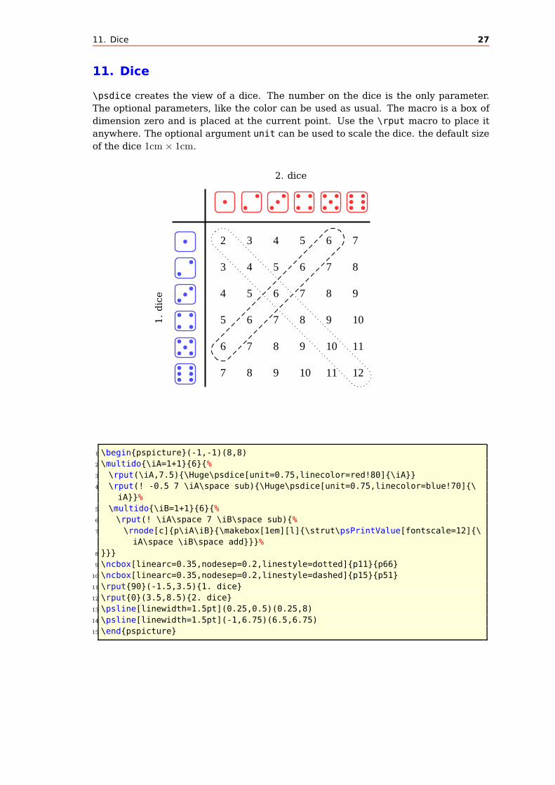
11. Dice 27
11. Dice
\psdice creates the view of a dice. The number on the dice is the only parameter.
The optional parameters, like the color can be used as usual. The macro is a box of
dimension zero and is placed at the current point. Use the \rput macro to place it
anywhere. The optional argument unit can be used to scale the dice. the default size
of the dice 1cm × 1cm.
2
3
4
5
6
7
3
4
5
6
7
8
4
5
6
7
8
9
5
6
7
8
9
10
6
7
8
9
10
11
7
8
9
10
11
12
1.dice
2. dice
1 \begin{pspicture}(-1,-1)(8,8)
2 \multido{\iA=1+1}{6}{%
3 \rput(\iA,7.5){\Huge\psdice[unit=0.75,linecolor=red!80]{\iA}}
4 \rput(! -0.5 7 \iA\space sub){\Huge\psdice[unit=0.75,linecolor=blue!70]{\
iA}}%
5 \multido{\iB=1+1}{6}{%
6 \rput(! \iA\space 7 \iB\space sub){%
7 \rnode[c]{p\iA\iB}{\makebox[1em][l]{\strut\psPrintValue[fontscale=12]{\
iA\space \iB\space add}}}%
8 }}}
9 \ncbox[linearc=0.35,nodesep=0.2,linestyle=dotted]{p11}{p66}
10 \ncbox[linearc=0.35,nodesep=0.2,linestyle=dashed]{p15}{p51}
11 \rput{90}(-1.5,3.5){1. dice}
12 \rput{0}(3.5,8.5){2. dice}
13 \psline[linewidth=1.5pt](0.25,0.5)(0.25,8)
14 \psline[linewidth=1.5pt](-1,6.75)(6.5,6.75)
15 \end{pspicture}

12. Arrows 28
12. Arrows
12.1. Definition
pstricks-add defines the following "‘arrows"’:
Value Example Name
- None
<-> Arrowheads.
>-< Reverse arrowheads.
<<->> Double arrowheads.
>>-<< Double reverse arrowheads.
|-| T-bars, flush to endpoints.
|*-|* T-bars, centered on endpoints.
[-] Square brackets.
]-[ Reversed square brackets.
(-) Rounded brackets.
)-( Reversed rounded brackets.
o-o Circles, centered on endpoints.
*-* Disks, centered on endpoints.
oo-oo Circles, flush to endpoints.
**-** Disks, flush to endpoints.
|<->| T-bars and arrows.
|>-<| T-bars and reverse arrows.
h-h| left/right hook arrows.
H-H| left/right hook arrows.
v-v| left/right inside vee arrows.
V-V| left/right outside vee arrows.
f-f| left/right inside filled arrows.
F-F| left/right outside filled arrows.
t-t| left/right inside slash arrows.
T-T| left/right outside slash arrows.
You can also mix and match, e.g., ->, *-) and [-> are all valid values of the arrows
parameter. The parameter can be set with
\psset{arrows=<type>}
or for some macros with a special option, like
\psline[<general options>]{<arrow type>}(A)(B)
\psline[linecolor=red,linewidth=2pt]{|->}(0,0)(0,2)
12.2. Multiple arrows
There are two new options which are only valid for the arrow type << or >>. nArrow
sets both, the nArrowA and the nArrowB parameter. The meaning is declared in the
following tables. Without setting one of these parameters the behaviour is like the
one described in the old PSTricks manual.

12.3. hookarrow 29
Value Meaning
->> -A
<<->> A-A
<<- A-
>>- B-
-<< -B
>>-<< B-B
>>->> B-A
<<-<< A-B
Value Example
\psline{->>}(0,1ex)(2.3,1ex)
\psline[nArrowsA=3]{->>}(0,1ex)(2.3,1ex)
\psline[nArrowsA=5]{->>}(0,1ex)(2.3,1ex)
\psline{<<-}(0,1ex)(2.3,1ex)
\psline[nArrowsA=3]{<<-}(0,1ex)(2.3,1ex)
\psline[nArrowsA=5]{<<-}(0,1ex)(2.3,1ex)
\psline{<<->>}(0,1ex)(2.3,1ex)
\psline[nArrowsA=3]{<<->>}(0,1ex)(2.3,1ex)
\psline[nArrowsA=5]{<<->>}(0,1ex)(2.3,1ex)
\psline{<<-|}(0,1ex)(2.3,1ex)
\psline[nArrowsA=3]{<<-<<}(0,1ex)(2.3,1ex)
\psline[nArrowsA=5]{<<-o}(0,1ex)(2.3,1ex)
\psline[nArrowsA=3,nArrowsB=4]{<<-<<}(0,1ex)(2.3,1ex)
\psline[nArrowsA=3,nArrowsB=4]{>>->>}(0,1ex)(2.3,1ex)
\psline[nArrowsA=1,nArrowsB=4]{>>->>}(0,1ex)(2.3,1ex)
12.3. hookarrow
R2
0 R3
eb : S 1 1 0
0
R1
er2 fr2
e1es
fse3f3 e4f4
e2f2e5
er3 fr3
er1 fr1
1 \psset{arrowsize=8pt,arrowlength=1,linewidth=1pt,nodesep=2pt,shortput=tablr}
2 \large
3 \begin{psmatrix}[colsep=12mm,rowsep=10mm]
4 & & $R_2$ \\
5 & & 0 & & $R_3$\\

12.4. hookrightarrow and hookleftarrow 30
6 $e_b:S$ & 1 & & 1 & 0 \\
7 & & 0 \\
8 & & $R_1$ \\
9 \end{psmatrix}
10 \ncline{h-}{1,3}{2,3}<{$e_{r2}$}>{$f_{r2}$}\ncline{-h}{2,3}{3,2}<{$e_1$}
11 \ncline{-h}{3,1}{3,2}^{$e_s$}_{$f_{s}$} \ncline{-h}{3,2}{4,3}>{$e_3$}<{$f_3$}
12 \ncline{-h}{4,3}{3,4}>{$e_4$}<{$f_4$} \ncline{-h}{3,4}{2,3}>{$e_2$}<{$f_2$}
13 \ncline{-h}{3,4}{3,5}^{$e_5$}
14 \ncline{-h}{3,5}{2,5}<{$e_{r3}$}>{$f_{r3}$}
15 \ncline{-h}{4,3}{5,3}<{$e_{r1}$}>{$f_{r1}$}
12.4. hookrightarrow and hookleftarrow
This is another type of arrow and is abbreviated with H. The length and width of the
hook is set by the new options hooklength and hookwidth, which are by default set
to
\psset{hooklength=3mm,hookwidth=1mm}
If the line begins with a right hook then the line ends with a left hook and vice versa:
1\begin{pspicture}(3,4)
2\psline[linewidth=5pt,linecolor=blue,hooklength=5mm,
hookwidth=-3mm]{H->}(0,3.5)(3,3.5)
3\psline[linewidth=5pt,linecolor=red,hooklength=5mm,
hookwidth=3mm]{H->}(0,2.5)(3,2.5)
4\psline[linewidth=5pt,hooklength=5mm,hookwidth=3mm]{H-H
}(0,1.5)(3,1.5)
5\psline[linewidth=1pt]{H-H}(0,0.5)(3,0.5)
6\end{pspicture}
E Wi(X) Y
Wj(X)
t
Wij s
1$\begin{psmatrix}
2E&W_i(X)&&Y\\
3&&W_j(X)
4\psset{arrows=->,nodesep=3pt,
linewidth=2pt}
5\everypsbox{\scriptstyle}
6\ncline[linecolor=red,arrows=H->,%
7 hooklength=4mm,hookwidth=2mm
]{1,1}{1,2}
8\ncline{1,2}{1,4}^{\tilde{t}}
9\ncline{1,2}{2,3}<{W_{ij}}
10\ncline{2,3}{1,4}>{\tilde{s}}
11\end{psmatrix}$
12.5. ArrowInside Option
It is now possible to have arrows inside lines and not only at the beginning or the end.
The new defined options

12.6. ArrowFill Option 31
Name Example Output
ArrowInside \psline[ArrowInside=->](0,0)(2,0)
ArrowInsidePos \psline[ArrowInside=->,%
ArrowInsidePos=0.25](0,0)(2,0)
ArrowInsidePos \psline[ArrowInside=->,%
ArrowInsidePos=10](0,0)(2,0)
ArrowInsideNo \psline[ArrowInside=->,%
ArrowInsideNo=2](0,0)(2,0)
ArrowInsideOffset \psline[ArrowInside=->,%
ArrowInsideNo=2,%
ArrowInsideOffset=0.1](0,0)(2,0)
ArrowInside \psline[ArrowInside=->]{->}(0,0)(2,0)
ArrowInsidePos \psline[ArrowInside=->,%
ArrowInsidePos=0.25]{->}(0,0)(2,0)
ArrowInsidePos \psline[ArrowInside=->,%
ArrowInsidePos=10]{->}(0,0)(2,0)
ArrowInsideNo \psline[ArrowInside=->,%
ArrowInsideNo=2]{->}(0,0)(2,0)
ArrowInsideOffset \psline[ArrowInside=->,%
ArrowInsideNo=2,%
ArrowInsideOffset=0.1]{->}(0,0)(2,0)
ArrowFill \psline[ArrowFill=false,%
arrowinset=0]{->}(0,0)(2,0)
ArrowFill \psline[ArrowFill=false,%
arrowinset=0]{«-»}(0,0)(2,0)
ArrowFill \psline[ArrowInside=->,%
arrowinset=0,%
ArrowFill=false,%
ArrowInsideNo=2,%
ArrowInsideOffset=0.1]{->}(0,0)(2,0)
Without the default arrow definition there is only the one inside the line, defined by
the type and the position. The position is relative to the length of the whole line. 0.25means at 25% of the line length. The peak of the arrow gets the coordinates which
are calculated by the macro. If you want arrows with an absolute position difference,
then choose a value greater than 1, e. g. 10 which places an arrow every 10 pt. The
default unit pt cannot be changed.
The ArrowInside takes only arrow definitions like -> into account. Arrows from
right to left (<-) are not possible and ignored. If you need such arrows, change the
order of the pairs of coordinates for the line or curve macro.
12.6. ArrowFill Option
By default all arrows are filled polygons. With the option ArrowFill=false there are
”white“ arrows. Only for the beginning/end arrows are they empty, the inside arrows
are overpainted by the line.

12.7. Examples 32
1\psset{arrowscale=2.5}
2\psline[linecolor=red,arrowinset=0]{<->}(-1,0)(2,0)
1\psset{arrowscale=2.5}
2\psline[linecolor=red,arrowinset=0,ArrowFill=false
]{<->}(-1,0)(2,0)
1\psset{arrowscale=2.5}
2\psline[linecolor=red,arrowinset=0,arrowsize=0.2,
3 ArrowFill=false]{<->}(-1,0)(2,0)
1\psline[linecolor=blue,arrowscale=4,
2 ArrowFill]{>>->>}(-1,0)(2,0)
1\psline[linecolor=blue,arrowscale=4,
2 ArrowFill=false]{>>->>}(-1,0)(2,0)
3\rule{3cm}{0pt}\\[30pt]
1\psline[linecolor=blue,arrowscale=4,
2 ArrowFill]{>|->|}(-1,0)(2,0)
1\psline[linecolor=blue,arrowscale=4,
2 ArrowFill=false]{>|->|}(-1,0)(2,0)%
12.7. Examples
All examples are printed with \psset{arrowscale=2,linecolor=red}.
\psline
1\begin{pspicture}(2,2)
2\psset{arrowscale=2,ArrowFill=true}
3\psline[ArrowInside=->]{|<->|}(2,1)
4\end{pspicture}
1\begin{pspicture}(2,2)
2\psset{arrowscale=2,ArrowFill=true}
3\psline[ArrowInside=-|]{|-|}(2,1)
4\end{pspicture}
1\begin{pspicture}(2,2)
2\psset{arrowscale=2,ArrowFill=true}
3\psline[ArrowInside=->,ArrowInsideNo=2]{->}(2,1)
4\end{pspicture}
1\begin{pspicture}(2,2)
2\psset{arrowscale=2,ArrowFill=true}
3\psline[ArrowInside=->,ArrowInsideNo=2,ArrowInsideOffset
=0.1]{->}(2,1)
4\end{pspicture}

12.7. Examples 33
1\begin{pspicture}(6,2)
2\psset{arrowscale=2,ArrowFill=true}
3\psline[ArrowInside=-*]{->}(0,0)(2,1)
(3,0)(4,0)(6,2)
4\end{pspicture}
1\begin{pspicture}(6,2)
2\psset{arrowscale=2,ArrowFill=true}
3\psline[ArrowInside=-*,ArrowInsidePos
=0.25]{->}(0,0)(2,1)(3,0)(4,0)(6,2)
4\end{pspicture}
1\begin{pspicture}(6,2)
2\psset{arrowscale=2,ArrowFill=true}
3\psline[ArrowInside=-*,ArrowInsidePos
=0.25,ArrowInsideNo=2]{->}%
4 (0,0)(2,1)(3,0)(4,0)(6,2)
5\end{pspicture}
1\begin{pspicture}(6,2)
2\psset{arrowscale=2,ArrowFill=true}
3\psline[ArrowInside=->, ArrowInsidePos
=0.25]{->}%
4 (0,0)(2,1)(3,0)(4,0)(6,2)
5\end{pspicture}
1\begin{pspicture}(6,2)
2\psset{arrowscale=2,ArrowFill=true}
3\psline[linestyle=none,ArrowInside=->,
ArrowInsidePos=0.25]{->}%
4 (0,0)(2,1)(3,0)(4,0)(6,2)
5\end{pspicture}
1\begin{pspicture}(6,2)
2\psset{arrowscale=2,ArrowFill=true}
3\psline[ArrowInside=-<, ArrowInsidePos
=0.75]{->}%
4 (0,0)(2,1)(3,0)(4,0)(6,2)
5\end{pspicture}
1\begin{pspicture}(6,2)
2\psset{arrowscale=2,ArrowFill=true,
ArrowInside=-*}
3\psline(0,0)(2,1)(3,0)(4,0)(6,2)
4\psset{linestyle=none}
5\psline[ArrowInsidePos=0](0,0)(2,1)(3,0)
(4,0)(6,2)
6\psline[ArrowInsidePos=1](0,0)(2,1)(3,0)
(4,0)(6,2)
7\end{pspicture}

12.7. Examples 34
1\begin{pspicture}(6,5)
2\psset{arrowscale=2,ArrowFill=true}
3\psline[ArrowInside=->,ArrowInsidePos
=20](0,0)(3,0)%
4 (3,3)(1,3)(1,5)(5,5)(5,0)(7,0)
(6,3)
5\end{pspicture}
1\begin{pspicture}(6,2)
2\psset{arrowscale=2,ArrowFill=true}
3\psline[ArrowInside=-|]{<->}(0,2)(2,0)
(3,2)(4,0)(6,2)
4\end{pspicture}
\pspolygon
1\begin{pspicture}(6,3)
2\psset{arrowscale=2}
3\pspolygon[ArrowInside=-|](0,0)(3,3)
(6,3)(6,1)
4\end{pspicture}
1\begin{pspicture}(6,3)
2\psset{arrowscale=2}
3\pspolygon[ArrowInside=->,ArrowInsidePos
=0.25]%
4 (0,0)(3,3)(6,3)(6,1)
5\end{pspicture}
1\begin{pspicture}(6,3)
2\psset{arrowscale=2}
3\pspolygon[ArrowInside=->,ArrowInsideNo
=4]%
4 (0,0)(3,3)(6,3)(6,1)
5\end{pspicture}
1\begin{pspicture}(6,3)
2\psset{arrowscale=2}
3\pspolygon[ArrowInside=->,ArrowInsideNo
=4,%
4 ArrowInsideOffset=0.1](0,0)(3,3)(6,3)
(6,1)
5\end{pspicture}

12.7. Examples 35
1\begin{pspicture}(6,3)
2\psset{arrowscale=2}
3 \pspolygon[ArrowInside=-|](0,0)(3,3)
(6,3)(6,1)
4 \psset{linestyle=none,ArrowInside=-*}
5 \pspolygon[ArrowInsidePos=0](0,0)(3,3)
(6,3)(6,1)
6 \pspolygon[ArrowInsidePos=1](0,0)(3,3)
(6,3)(6,1)
7 \psset{ArrowInside=-o}
8 \pspolygon[ArrowInsidePos=0.25](0,0)
(3,3)(6,3)(6,1)
9 \pspolygon[ArrowInsidePos=0.75](0,0)
(3,3)(6,3)(6,1)
10\end{pspicture}
1\begin{pspicture}(6,5)
2\psset{arrowscale=2}
3 \pspolygon[ArrowInside=->,
ArrowInsidePos=20]%
4 (0,0)(3,0)(3,3)(1,3)(1,5)(5,5)(5,0)
(7,0)(6,3)
5\end{pspicture}
\psbezier
1\begin{pspicture}(3,3)
2\psset{arrowscale=2}
3 \psbezier[ArrowInside=-|](0,1)(1,0)(2,1)(3,3)
4 \psset{linestyle=none,ArrowInside=-o}
5 \psbezier[ArrowInsidePos=0.25](0,1)(1,0)(2,1)(3,3)
6 \psbezier[ArrowInsidePos=0.75](0,1)(1,0)(2,1)(3,3)
7 \psset{linestyle=none,ArrowInside=-*}
8 \psbezier[ArrowInsidePos=0](0,1)(1,0)(2,1)(3,3)
9 \psbezier[ArrowInsidePos=1](0,1)(1,0)(2,1)(3,3)
10\end{pspicture}
b
b
1\begin{pspicture}(4,3)
2\psset{arrowscale=2}
3 \psbezier[ArrowInside=->,showpoints=true]%
4 {*-*}(0,0)(2,3)(3,0)(4,2)
5\end{pspicture}
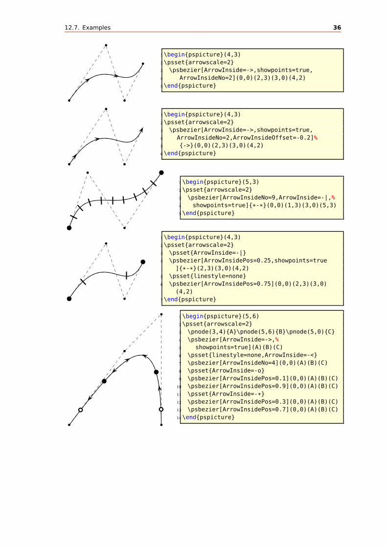
12.7. Examples 36
b
b
b
b
1\begin{pspicture}(4,3)
2\psset{arrowscale=2}
3 \psbezier[ArrowInside=->,showpoints=true,
4 ArrowInsideNo=2](0,0)(2,3)(3,0)(4,2)
5\end{pspicture}
b
b
b
1\begin{pspicture}(4,3)
2\psset{arrowscale=2}
3 \psbezier[ArrowInside=->,showpoints=true,
4 ArrowInsideNo=2,ArrowInsideOffset=-0.2]%
5 {->}(0,0)(2,3)(3,0)(4,2)
6\end{pspicture}
b
b
1\begin{pspicture}(5,3)
2\psset{arrowscale=2}
3 \psbezier[ArrowInsideNo=9,ArrowInside=-|,%
4 showpoints=true]{*-*}(0,0)(1,3)(3,0)(5,3)
5\end{pspicture}
b
b
1\begin{pspicture}(4,3)
2\psset{arrowscale=2}
3 \psset{ArrowInside=-|}
4 \psbezier[ArrowInsidePos=0.25,showpoints=true
]{*-*}(2,3)(3,0)(4,2)
5 \psset{linestyle=none}
6 \psbezier[ArrowInsidePos=0.75](0,0)(2,3)(3,0)
(4,2)
7\end{pspicture}
b
b
b
b
1\begin{pspicture}(5,6)
2\psset{arrowscale=2}
3 \pnode(3,4){A}\pnode(5,6){B}\pnode(5,0){C}
4 \psbezier[ArrowInside=->,%
5 showpoints=true](A)(B)(C)
6 \psset{linestyle=none,ArrowInside=-<}
7 \psbezier[ArrowInsideNo=4](0,0)(A)(B)(C)
8 \psset{ArrowInside=-o}
9 \psbezier[ArrowInsidePos=0.1](0,0)(A)(B)(C)
10 \psbezier[ArrowInsidePos=0.9](0,0)(A)(B)(C)
11 \psset{ArrowInside=-*}
12 \psbezier[ArrowInsidePos=0.3](0,0)(A)(B)(C)
13 \psbezier[ArrowInsidePos=0.7](0,0)(A)(B)(C)
14\end{pspicture}

12.7. Examples 37
b
b
b
1\begin{pspicture}(-3,-5)(15,5)
2 \psbezier[ArrowInsideNo=19,%
3 ArrowInside=->,ArrowFill=false,%
4 showpoints=true]{->}(-3,0)(5,-5)(8,5)(15,-5)
5\end{pspicture}
\pcline
These examples need the package pst-node.
1\begin{pspicture}(2,1)
2\psset{arrowscale=2}
3\pcline[ArrowInside=->](0,0)(2,1)
4\end{pspicture}
1\begin{pspicture}(2,1)
2\psset{arrowscale=2}
3\pcline[ArrowInside=->]{<->}(0,0)(2,1)
4\end{pspicture}
1\begin{pspicture}(2,1)
2\psset{arrowscale=2}
3\pcline[ArrowInside=-|,ArrowInsidePos=0.75]{|-|}(0,0)(2,1)
4\end{pspicture}
g 1\psset{arrowscale=2}
2\pcline[ArrowInside=->,ArrowInsidePos=0.65]{*-*}(0,0)(2,0)
3\naput[labelsep=0.3]{\large$g$}

12.7. Examples 38
l 1\psset{arrowscale=2}
2\pcline[ArrowInside=->,ArrowInsidePos=10]{|-|}(0,0)(2,0)
3\naput[labelsep=0.3]{\large$l$}
\pccurve
These examples also need the package pst-node.
h
1\begin{pspicture}(2,2)
2\psset{arrowscale=2}
3\pccurve[ArrowInside=->,ArrowInsidePos=0.65,showpoints=true
]{*-*}(0,0)(2,2)
4\naput[labelsep=0.3]{\large$h$}
5\end{pspicture}
i
1\begin{pspicture}(2,2)
2\psset{arrowscale=2}
3\pccurve[ArrowInside=->,ArrowInsideNo=3,showpoints=true
]{|->}(0,0)(2,2)
4\naput[labelsep=0.3]{\large$i$}
5\end{pspicture}
k
1\begin{pspicture}(4,4)
2\psset{arrowscale=2}
3\pccurve[ArrowInside=->,ArrowInsidePos
=20]{|-|}(0,0)(4,4)
4\naput[labelsep=0.3]{\large$k$}
5\end{pspicture}

12.8. Special arrows v-V,t-T, and f-F 39
12.8. Special arrows v-V,t-T, and f-F
Possible optional arguments are
name meaning
veearrowlength default is 3mm
veearrowangle default is 30
veearrowlinewidth default is 0.35mm
filledveearrowlength default is 3mm
filledveearrowangle default is 15
filledveearrowlinewidth default is 0.35mm
tickarrowlength default is 1.5mm
tickarrowlinewidth default is 0.35mm
1\psset{unit=5mm}
2\begin{pspicture}(4,6)
3 \psset{dimen=middle,arrows=c-c,
4 arrowscale=2,linewidth=.25mm}
5 \psline[linecolor=red,linewidth=.05mm](0,0)(0,6)
6 \psline[linecolor=red,linewidth=.05mm](4,0)(4,6)
7 \psline{v-v}(0,6)(4,6)
8 \psline{v-V}(0,4)(4,4)
9 \psline{V-v}(0,2)(4,2)
10 \psline{V-V}(0,0)(4,0)
11\end{pspicture}
1\psset{unit=5mm}
2\begin{pspicture}(4,6)
3 \psset{dimen=middle,arrows=c-c,
4 arrowscale=2,linewidth=.25mm}
5 \psline[linecolor=red,linewidth=.05mm](0,0)(0,6)
6 \psline[linecolor=red,linewidth=.05mm](4,0)(4,6)
7 \psline{f-f}(0,6)(4,6)
8 \psline{f-F}(0,4)(4,4)
9 \psline{F-f}(0,2)(4,2)
10 \psline{F-F}(0,0)(4,0)
11\end{pspicture}
1\psset{unit=5mm}
2\begin{pspicture}(4,6)
3 \psset{dimen=middle,arrows=c-c,linewidth=.25mm}
4 \psline[linecolor=red,linewidth=.05mm](0,0)(0,6)
5 \psline[linecolor=red,linewidth=.05mm](4,0)(4,6)
6 \psline{t-t}(0,6)(4,6)
7 \psline{t-T}(0,4)(4,4)
8 \psline{T-t}(0,2)(4,2)
9 \psline{T-T}(0,0)(4,0)
10\end{pspicture}
12.9. Special arrow option arrowLW
Only for the arrowtype o and * it is possible to set the arrowlinewidth with the optional
keyword arrowLW. When scaling an arrow by the keyword arrowscale the width of the

12.9. Special arrow option arrowLW 40
borderline is also scaled. With the optional argument arrowLW the line width can be
set separately and is not taken into account by the scaling value.
1\begin{pspicture}(4,6)
2\psline[arrowscale=3,arrows=*-o](0,5)(4,5)
3\psline[arrowscale=3,arrows=*-o,
4 arrowLW=0.5pt](0,3)(4,3)
5\psline[arrowscale=3,arrows=*-o,
6 arrowLW=0.3333\pslinewidth](0,1)(4,1)
7\end{pspicture}

13. \psFormatInt 41
13. \psFormatInt
There exist some packages and a lot of code to format an integer like 1 000 000 or
1, 234, 567 (in Europe 1.234.567). But all packages expect a real number as argument
and cannot handle macros as an argument. For this case pstricks-add has a macro
\psFormatInt which can handle both:
1,234,567
1,234,567
1.234.567
1·234·567965,432
1\psFormatInt{1234567}\\
2\psFormatInt[intSeparator={,}]{1234567}\\
3\psFormatInt[intSeparator=.]{1234567}\\
4\psFormatInt[intSeparator=$\cdot$]{1234567}\\
5\def\temp{965432}
6\psFormatInt{\temp}
With the option intSeparator the symbol can be changed to any any non-number
character.
14. Color
14.1. Transparent colors
Transparency is now part of the main pstricks package. But pay attention, the names
and syntax have changed and you need to run ps2pdf with the option -dCompatibilityLevel=1.4.
14.2. „Manipulating transparent colors”
pstricks-add supports real transparency and a simulated one with hatch lines:
1 \def\defineTColor{\@ifnextchar[{\defineTColor@i}{\defineTColor@i[]}}
2 \def\defineTColor@i[#1]#2#3{% transparency "Colors"
3 \newpsstyle{#2}{%
4 fillstyle=vlines,hatchwidth=0.1\pslinewidth,
5 hatchsep=1\pslinewidth,hatchcolor=#3,#1%
6 }%
7 }
8 \defineTColor{TRed}{red}
9 \defineTColor{TGreen}{green}
10 \defineTColor{TBlue}{blue}
There are three predefined "’transparent"‘ colors TRed, TGreen, TBlue. They are
used as PSTricks styles and not as colors:

14.3. Calculated colors 42
+
1\begin{pspicture}(-3,-5)(5,5)
2\psframe(-1,-3)(5,5) % objet de base
3\psrotate(2,-2){15}{%
4 \psframe[style=TRed](-1,-3)(5,5)}
5\psrotate(2,-2){30}{%
6 \psframe[style=TGreen](-1,-3)(5,5)}
7\psrotate(2,-2){45}{%
8 \psframe[style=TBlue](-1,-3)(5,5)}
9\psframe[linewidth=3pt](-1,-3)(5,5)
10\psdots[dotstyle=+,dotangle=45,dotscale=3](2,-2) % centre de la rotation
11\end{pspicture}
14.3. Calculated colors
The xcolor package (version 2.6) has a new feature for defining colors:
\definecolor[ps]{<name>}{<model>}{< PS code >}
model can be one of the color models, which PostScript will understand, e.g. rgb.
With this definition the color is calculated on the PostScript side.

14.3. Calculated colors 43
350 400 450 500 550 600 650 700 750 λ[nm]
1\definecolor[ps]{bl}{rgb}{tx@addDict begin Red Green Blue end}%
2\psset{unit=1bp}
3\begin{pspicture}(0,-30)(400,100)
4\multido{\iLAMBDA=0+1}{400}{%
5 \pstVerb{
6 \iLAMBDA\space 379 add dup /lambda exch def
7 tx@addDict begin wavelengthToRGB end
8 }%
9 \psline[linecolor=bl](\iLAMBDA,0)(\iLAMBDA,100)%
10}
11\psaxes[yAxis=false,Ox=350,dx=50bp,Dx=50]{->}(-29,-10)(420,100)
12\uput[-90](420,-10){$\lambda$[\textsf{nm}]}
13\end{pspicture}
380 420 460 500 540 580 620 660 700 740 780λ(nm)
380 420 460 500 540 580 620 660 700 740 780λ(nm)
Spectrum of hydrogen emission (Manuel Luque)
1 \newcommand{\Touch}{%
2 \psframe[linestyle=none,fillstyle=solid,fillcolor=bl,dimen=middle](0.1,0.75)
}
3 \definecolor[ps]{bl}{rgb}{tx@addDict begin Red Green Blue end}%
4 % Echelle 1cm <-> 40 nm
5 % 1 nm <-> 0.025 cm
6 \psframebox[fillstyle=solid,fillcolor=black]{%
7 \begin{pspicture}(-1,-0.5)(12,1.5)
8 \multido{\iLAMBDA=380+2}{200}{%
9 \pstVerb{
10 /lambda \iLAMBDA\space def
11 lambda
12 tx@addDict begin wavelengthToRGB end
13 }%
14 \rput(! lambda 0.025 mul 9.5 sub 0){\Touch}

14.4. Gouraud shading 44
15 }
16 \multido{\n=0+1,\iDiv=380+40}{11}{%
17 \psline[linecolor=white](\n,0.1)(\n,-0.1)
18 \uput[270](\n,0){\textbf{\white\iDiv}}}
19 \psline[linecolor=white]{->}(11,0)
20 \uput[270](11,0){\textbf{\white$\lambda$(nm)}}
21 \end{pspicture}}
22
23 \psframebox[fillstyle=solid,fillcolor=black]{%
24 \begin{pspicture}(-1,-0.5)(12,1)
25 \pstVerb{
26 /lambda 656 def
27 lambda
28 tx@addDict begin wavelengthToRGB end
29 }%
30 \rput(! 656 0.025 mul 9.5 sub 0){\Touch}
31 \pstVerb{
32 /lambda 486 def
33 lambda
34 tx@addDict begin wavelengthToRGB end
35 }%
36 \rput(! 486 0.025 mul 9.5 sub 0){\Touch}
37 \pstVerb{
38 /lambda 434 def
39 lambda
40 tx@addDict begin wavelengthToRGB end
41 }%
42 \rput(! 434 0.025 mul 9.5 sub 0){\Touch}
43 \pstVerb{
44 /lambda 410 def
45 lambda
46 tx@addDict begin wavelengthToRGB end
47 }%
48 \rput(! 410 0.025 mul 9.5 sub 0){\Touch}
49 \multido{\n=0+1,\iDiv=380+40}{11}{%
50 \psline[linecolor=white](\n,0.1)(\n,-0.1)
51 \uput[270](\n,0){\textbf{\white\iDiv}}}
52 \psline[linecolor=white]{->}(11,0)
53 \uput[270](11,0){\textbf{\white$\lambda$(nm)}}
54 \end{pspicture}}
55
56 Spectrum of hydrogen emission (Manuel Luque)
14.4. Gouraud shading
Gouraud shading is a method used in computer graphics to simulate
the differing effects of light and colour across the surface of an object.
In practice, Gouraud shading is used to achieve smooth lighting on low-
polygon surfaces without the heavy computational requirements of calcu-
lating lighting for each pixel. The technique was first presented by Henri
Gouraud in 1971.

14.4. Gouraud shading 45
http://www.wikipedia.org
PostScript level 3 supports this kind of shading and it can only be seen with Acroread
7 or later. The syntax is easy:
\psGTriangle(x1,y1)(x2,y2)(x3,y3){color1}{color2}{color3}
1\begin{pspicture}(0,-.25)(10,10)
2 \psGTriangle(0,0)(5,10)(10,0){red}{green}{blue}
3\end{pspicture}
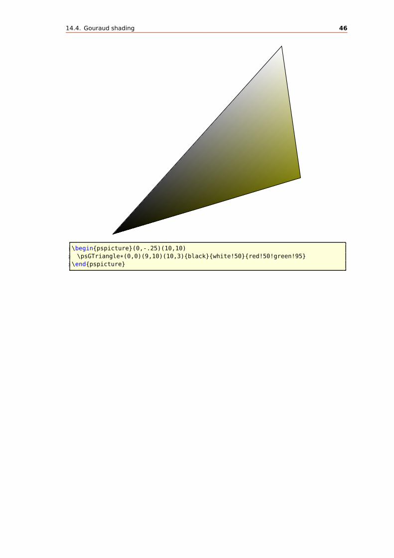
14.4. Gouraud shading 46
1\begin{pspicture}(0,-.25)(10,10)
2 \psGTriangle*(0,0)(9,10)(10,3){black}{white!50}{red!50!green!95}
3\end{pspicture}

14.4. Gouraud shading 47
1\begin{pspicture}(0,-.25)(10,10)
2 \psGTriangle*(0,0)(5,10)(10,0){-red!100!green!84!blue!86}
3 {-red!80!green!100!blue!40}
4 {-red!60!green!30!blue!100}
5\end{pspicture}

14.4. Gouraud shading 48
1\definecolor{rose}{rgb}{1.00, 0.84, 0.88}
2\definecolor{vertpommepasmure}{rgb}{0.80, 1.0, 0.40}
3\definecolor{fushia}{rgb}{0.60, 0.30, 1.0}
4\begin{pspicture}(0,-.25)(10,10)
5 \psGTriangle(0,0)(5,10)(10,0){rose}{vertpommepasmure}{fushia}
6\end{pspicture}
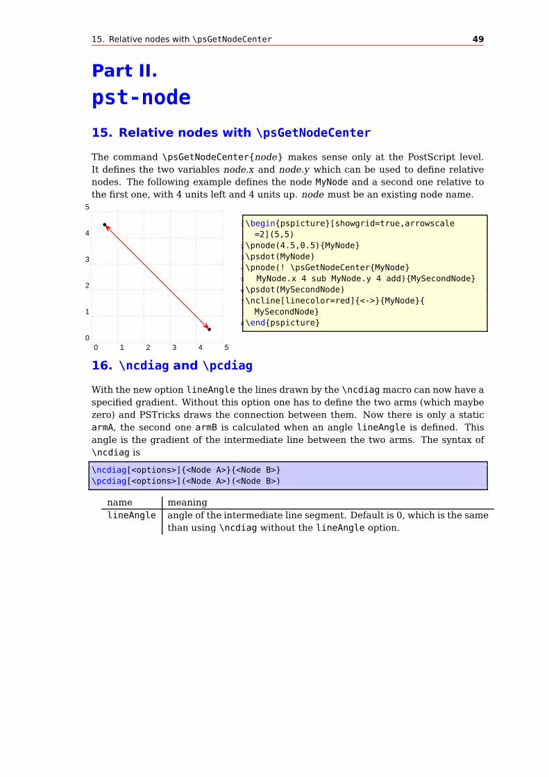
15. Relative nodes with \psGetNodeCenter 49
Part II.
pst-node
15. Relative nodes with \psGetNodeCenter
The command \psGetNodeCenter{node} makes sense only at the PostScript level.
It defines the two variables node.x and node.y which can be used to define relative
nodes. The following example defines the node MyNode and a second one relative to
the first one, with 4 units left and 4 units up. node must be an existing node name.
0 1 2 3 4 50
1
2
3
4
5
b
b 1\begin{pspicture}[showgrid=true,arrowscale
=2](5,5)
2\pnode(4.5,0.5){MyNode}
3\psdot(MyNode)
4\pnode(! \psGetNodeCenter{MyNode}
5 MyNode.x 4 sub MyNode.y 4 add){MySecondNode}
6\psdot(MySecondNode)
7\ncline[linecolor=red]{<->}{MyNode}{
MySecondNode}
8\end{pspicture}
16. \ncdiag and \pcdiag
With the new option lineAngle the lines drawn by the \ncdiag macro can now have a
specified gradient. Without this option one has to define the two arms (which maybe
zero) and PSTricks draws the connection between them. Now there is only a static
armA, the second one armB is calculated when an angle lineAngle is defined. This
angle is the gradient of the intermediate line between the two arms. The syntax of
\ncdiag is
\ncdiag[<options>]{<Node A>}{<Node B>}
\pcdiag[<options>](<Node A>)(<Node B>)
name meaning
lineAngle angle of the intermediate line segment. Default is 0, which is the same
than using \ncdiag without the lineAngle option.

16. \ncdiag and \pcdiag 50
A C E
B
D
F
lineIline
IIline
III
1\begin{pspicture}(5,6)
2 \circlenode{A}{A}\quad\circlenode{C}{C}%
3 \quad\circlenode{E}{E}
4 \rput(0,4){\circlenode{B}{B}}
5 \rput(1,5){\circlenode{D}{D}}
6 \rput(2,6){\circlenode{F}{F}}
7 \psset{arrowscale=2,linearc=0.2,%
8 linecolor=red,armA=0.5, angleA=90,angleB
=-90}
9 \ncdiag[lineAngle=20]{->}{A}{B}
10 \ncput*[nrot=:U]{line I}
11 \ncdiag[lineAngle=20]{->}{C}{D}
12 \ncput*[nrot=:U]{line II}
13 \ncdiag[lineAngle=20]{->}{E}{F}
14 \ncput*[nrot=:U]{line III}
15\end{pspicture}
The \ncdiag macro sets the armB dynamically to the calculated value. Any user
setting of armB is overwritten by the macro. The armA could be set to a zero length:
A
B1\begin{pspicture}(4,3)
2 \rput(0.5,0.5){\circlenode{A}{A}}
3 \rput(3.5,3){\circlenode{B}{B}}
4 {\psset{linecolor=red,arrows=<-,arrowscale=2}
5 \ncdiag[lineAngle=60,%
6 armA=0,angleA=0,angleB=180]{A}{B}
7 \ncdiag[lineAngle=60,%
8 armA=0,angleA=90,angleB=180]{A}{B}}
9\end{pspicture}
A
B
1\begin{pspicture}(4,3)
2 \rput(1,0.5){\circlenode{A}{A}}
3 \rput(4,3){\circlenode{B}{B}}
4 {\psset{linecolor=red,arrows=<-,arrowscale=2}
5 \ncdiag[lineAngle=60,%
6 armA=0.5,angleA=0,angleB=180]{A}{B}
7 \ncdiag[lineAngle=60,%
8 armA=0,angleA=70,angleB=180]{A}{B}
9 \ncdiag[lineAngle=60,%
10 armA=0.5,angleA=180,angleB=180]{A}{B}}
11\end{pspicture}

17. \ncdiagg and \pcdiagg 51
1\begin{pspicture}(4,5.5)
2 \cnode*(0,0){2pt}{A}%
3 \cnode*(0.25,0){2pt}{C}%
4 \cnode*(0.5,0){2pt}{E}%
5 \cnode*(0.75,0){2pt}{G}%
6 \cnode*(2,4){2pt}{B}%
7 \cnode*(2.5,4.5){2pt}{D}%
8 \cnode*(3,5){2pt}{F}%
9 \cnode*(3.5,5.5){2pt}{H}%
10 {\psset{arrowscale=2,linearc=0.2,%
11 linecolor=red,armA=0.5, angleA=90,angleB=-90}
12 \pcdiag[lineAngle=20]{->}(A)(B)
13 \pcdiag[lineAngle=20]{->}(C)(D)
14 \pcdiag[lineAngle=20]{->}(E)(F)
15 \pcdiag[lineAngle=20]{->}(G)(H)}
16\end{pspicture}
17. \ncdiagg and \pcdiagg
This is nearly the same as \ncdiag except that armB=0 and the angleB value is com-
puted by the macro, so that the line ends at the node with an angle like a \pcdiagg
line. The syntax of \ncdiagg/\pcdiagg is
\ncdiag[<options>]{<Node A>}{<Node B>}
\pcdiag[<options>](<Node A>)(<Node B>)
A C E
B
D
F
lineI
lineII
lineIII
1\begin{pspicture}(4,6)
2 \psset{linecolor=black}
3 \circlenode{A}{A}%
4 \quad\circlenode{C}{C}%
5 \quad\circlenode{E}{E}
6 \rput(0,4){\circlenode{B}{B}}
7 \rput(1,5){\circlenode{D}{D}}
8 \rput(2,6){\circlenode{F}{F}}
9 {\psset{arrowscale=2,linearc=0.2,linecolor=red
,armA=0.5, angleA=90}
10 \ncdiagg[lineAngle=-160]{->}{A}{B}
11 \ncput*[nrot=:U]{line I}
12 \ncdiagg[lineAngle=-160]{->}{C}{D}
13 \ncput*[nrot=:U]{line II}
14 \ncdiagg[lineAngle=-160]{->}{E}{F}
15 \ncput*[nrot=:U]{line III}}
16\end{pspicture}

18. \ncbarr 52
1\begin{pspicture}(4,6)
2 \psset{linecolor=black}
3 \cnode*(0,0){2pt}{A}%
4 \cnode*(0.25,0){2pt}{C}%
5 \cnode*(0.5,0){2pt}{E}%
6 \cnode*(0.75,0){2pt}{G}%
7 \cnode*(2,4){2pt}{B}%
8 \cnode*(2.5,4.5){2pt}{D}%
9 \cnode*(3,5){2pt}{F}%
10 \cnode*(3.5,5.5){2pt}{H}%
11 {\psset{arrowscale=2,linearc=0.2,linecolor=red
,armA=0.5, angleA=90}
12 \pcdiagg[lineAngle=20]{->}(A)(B)
13 \pcdiagg[lineAngle=20]{->}(C)(D)
14 \pcdiagg[lineAngle=20]{->}(E)(F)
15 \pcdiagg[lineAngle=20]{->}(G)(H)}
16\end{pspicture}
The only catch for \ncdiagg is that you need the right value for lineAngle. If the
node connection is on the wrong side of the second node, then choose the correspond-
ing angle, e. g.: if 20 is wrong then take −160, which differs by 180.
A
H
1\begin{pspicture}(4,1.5)
2 \circlenode{a}{A}
3 \rput[l](3,1){\rnode{b}{H}}
4 \ncdiagg[lineAngle=60,angleA=180,armA=.5,nodesepA=3
pt,linecolor=blue]{b}{a}
5\end{pspicture}
A
H
1\begin{pspicture}(4,1.5)
2 \circlenode{a}{A}
3 \rput[l](3,1){\rnode{b}{H}}
4 \ncdiagg[lineAngle=60,armA=.5,nodesepB=3pt,
linecolor=blue]{a}{b}
5\end{pspicture}
A
H
1\begin{pspicture}(4,1.5)
2 \circlenode{a}{A}
3 \rput[l](3,1){\rnode{b}{H}}
4 \ncdiagg[lineAngle=-120,armA=.5,nodesepB=3pt,
linecolor=blue]{a}{b}
5\end{pspicture}
18. \ncbarr
This has the same behaviour as \ncbar, but has 5 segments and all are horizontal
ones. This is the reason why angleA must be 0 or alternatively 180. All other valuesare set to 0 by the macro. The intermediate horizontal line is symmetrical to the
distance of the two nodes.

19. \psRelNode and \psDefPSPNodes 53
X
Y
1\psset{arrowscale=2}%
2\circlenode{X}{X}\\[1cm]
3\circlenode{Y}{Y}
4\ncbarr[angleA=0,arrows=->,arrowscale=2]{X}{Y}
Xxxxx
Yyyy
1\psset{arrowscale=2}%
2\ovalnode{X}{Xxxxx}\\[1cm]
3\circlenode{Y}{Yyyy}
4\ncbarr[angleA=180,arrows=->,arrowscale=2,linecolor=red
]{X}{Y}
Xxxxx
Yyyy
1\psset{arrowscale=2}%
2\ovalnode{X}{Xxxxx}\\[1cm]
3\circlenode{Y}{Yyyy}
4\ncbarr[angleA=20,arm=1cm,arrows=->,arrowscale=2]{X}{Y}
19. \psRelNode and \psDefPSPNodes
With these macros it is possible to put a node relative to a given line or given pspicture-
environment. In the frist case the parameters are the angle and the length factor:
\psRelNode(<P0>)(<P1>){<length factor>}{<end node name>}
\psRelLine[<options>](<P0>)(<P1>){<length factor>}{<end node name>}
The length factor relates to the distance P0P1 and the end node name must be a
valid nodename and shouldn’t contain any of the special PostScript characters. There
are two valid options:name default meaning
angle 0 angle between the given line P0P1 and the new one P0PendNode
trueAngle false defines whether the angle refers to the seen line or to the
mathematical one, which respect the scaling factors xunit and
yunit.
0
30
60
90
120150
180
210
240
270
300 330
1\begin{pspicture}(7,6)
2 \psgrid[gridwidth=0pt,gridcolor=
gray,gridlabels=0pt,subgriddiv=2]
3 \pnode(3,3){A}\pnode(4,2){B}
4 \psline[nodesep=-3,linewidth=0.5pt
](A)(B)
5 \multido{\iA=0+30}{12}{%
6 \psRelNode[angle=\iA](A)(B){2}{C}%
7 \qdisk(C){2pt}
8 \uput[0](C){\iA}}
9\end{pspicture}

20. \psRelLine 54
In the second case the new macro \psDefPSPNodes defines nine nodes that cor-
responds to nine particular points (namely bottom left, bottom center, bottom right,
center left, center center, center right, top left, top center, top right) of the pspicture
box.
-1 0 1 2 3 4-1
0
1
2
3
4
b b b
b b b
b b b
PSPbl PSPbc PSPbr
PSPcl PSPcc PSPcr
PSPtl PSPtc PSPtr
1\begin{pspicture}[showgrid=true](-1,-1)
(4,4)
2 \psDefPSPNodes
3 \psdots(PSPbl)(PSPbc)(PSPbr)
4 (PSPcl)(PSPcc)(PSPcr)(PSPtl)(PSPtc)(
PSPtr)
5 \uput[90](PSPbl){PSPbl} \uput[90](PSPbc){
PSPbc}
6 \uput[90](PSPbr){PSPbr} \uput[90](PSPcl){
PSPcl}
7 \uput[90](PSPcc){PSPcc} \uput[90](PSPcr){
PSPcr}
8 \uput[90](PSPtl){PSPtl} \uput[90](PSPtc){
PSPtc}
9 \uput[90](PSPtr){PSPtr}
10\end{pspicture}
The name of the nodes are predefined as:
\psset[pst-PSPNodes]{blName=PSPbl,bcName=PSPbc,brName=PSPbr,
clName=PSPcl,ccName=PSPcc,crName=PSPcr,tlName=PSPtl,tcName=PSPtc,trName=PSPtr
}
and can be modified in the same way.
20. \psRelLine
With this macro it is possible to plot lines relative to a given one. Parameter are the
angle and the length factor:
\psRelLine(P0)(P1){length factor}{<end node name>}
\psRelLine [{arrows}] (P0)(P1){length factor}{end node name}
\psRelLine [Options] (P0)(P1){length factor}{end node name}
\psRelLine [Options] [{arrows}] (P0)(P1){length factor}{end node name}
The length factor relates to the distance P0P1 and the end node name must be a valid
nodename and shouldn’t contain any of the special PostScript characters. There are
two valid options which are described in the foregoing section for \psRelNode.
The following two figures show the same, the first one with a scaling different to
1 : 1, this is the reason why the end points are on an ellipse and not on a circle like in
the second figure.

20. \psRelLine 55
-2 -1 0 1 2 3-2
-1
0
1
21\psset{yunit=2,xunit=1}
2\begin{pspicture}(-2,-2)(3,2)
3\psgrid[subgriddiv=2,subgriddots=10,gridcolor=
lightgray]
4\pnode(-1,0){A}\pnode(3,2){B}
5\psline[linecolor=red](A)(B)
6\psRelLine[linecolor=blue,angle=30](-1,0)(B)
{0.5}{EndNode}
7\qdisk(EndNode){2pt}
8\psRelLine[linecolor=blue,angle=-30](A)(B)
{0.5}{EndNode}
9\qdisk(EndNode){2pt}
10\psRelLine[linecolor=magenta,angle=90](-1,0)
(3,2){0.5}{EndNode}
11\qdisk(EndNode){2pt}
12\psRelLine[linecolor=magenta,angle=-90](A)(B)
{0.5}{EndNode}
13\qdisk(EndNode){2pt}
14\end{pspicture}
-2 -1 0 1 2 3-2
-1
0
1
2
1\begin{pspicture}(-2,-2)(3,2)
2\psgrid[subgriddiv=2,subgriddots=10,gridcolor=
lightgray]
3\pnode(-1,0){A}\pnode(3,2){B}
4\psline[linecolor=red](A)(B)
5\psarc[linestyle=dashed](A){2.23}{-90}{135}
6\psRelLine[linecolor=blue,angle=30](-1,0)(B)
{0.5}{EndNode}
7\qdisk(EndNode){2pt}
8\psRelLine[linecolor=blue,angle=-30](A)(B)
{0.5}{EndNode}
9\qdisk(EndNode){2pt}
10\psRelLine[linecolor=magenta,angle=90](-1,0)
(3,2){0.5}{EndNode}
11\qdisk(EndNode){2pt}
12\psRelLine[linecolor=magenta,angle=-90](A)(B)
{0.5}{EndNode}
13\qdisk(EndNode){2pt}
14\end{pspicture}
The following figure has also a different scaling, but has set the option trueAngle,
all angles refer to "what you see".

20. \psRelLine 56
-3 -2 -1 0 1 2 3-1
0
1
2
1\psset{yunit=2,xunit=1}
2\begin{pspicture}(-3,-1)(3,2)\psgrid[
subgridcolor=lightgray]
3\pnode(-1,0){A}\pnode(3,2){B}
4\psline[linecolor=red](A)(B)
5\psarc(A){2.83}{-45}{135}
6\psRelLine[linecolor=blue,angle=30,
trueAngle](A)(B){0.5}{EndNode}
7\qdisk(EndNode){2pt}
8\psRelLine[linecolor=blue,angle=-30,
trueAngle](A)(B){0.5}{EndNode}
9\qdisk(EndNode){2pt}
10\psRelLine[linecolor=magenta,angle=90,
trueAngle](A)(B){0.5}{EndNode}
11\qdisk(EndNode){2pt}
12\psRelLine[linecolor=magenta,angle=-90,
trueAngle](A)(B){0.5}{EndNode}
13\qdisk(EndNode){2pt}
14\end{pspicture}
Two examples using \multido to show the behaviour of the options trueAngle and
angle.
-1 0 1 2 30
1
2
1\psset{yunit=4,xunit=2}
2\begin{pspicture}(-1,0)(3,2)\
psgrid[subgridcolor=lightgray]
3\pnode(-1,0){A}\pnode(1,1){B}
4\psline[linecolor=red](A)(3,2)
5\multido{\iA=0+10}{36}{%
6 \psRelLine[linecolor=blue,
angle=\iA](B)(A){-0.5}{
EndNode}
7 \qdisk(EndNode){2pt}
8}
9\end{pspicture}

20. \psRelLine 57
-1 0 1 2 30
1
2
1\psset{yunit=4,xunit=2}
2\begin{pspicture}(-1,0)(3,2)\
psgrid[subgridcolor=lightgray]
3\pnode(-1,0){A}\pnode(1,1){B}
4\psline[linecolor=red](A)(3,2)
5\multido{\iA=0+10}{36}{%
6 \psRelLine[linecolor=magenta,
angle=\iA,trueAngle]{->}(B)(
A){-0.5}{EndNode}
7}
8\end{pspicture}
Anström
richtung
v∞
FH
FV FR
FN
FT
1 \psset{xunit=0.75\linewidth,yunit=0.75\linewidth,trueAngle}%
2 \end{center}
3 \begin{pspicture}(1,0.6)%\psgrid
4 \pnode(.3,.35){Vk} \pnode(.375,.35){D} \pnode(0,.4){DST1} \pnode(1,.18){
DST2}
5 \pnode(0,.1){A1} \pnode(1,.31){A1}
6 { \psset{linewidth=.02,linestyle=dashed,linecolor=gray}%
7 \pcline(DST1)(DST2) % <- Druckseitentangente
8 \pcline(A2)(A1) % <- Anstr"omrichtung
9 \lput*{:U}{\small Anstr"omrichtung $v_{\infty}$} }%
10 \psIntersectionPoint(A1)(A2)(DST1)(DST2){Hk}
11 \pscurve(Hk)(.4,.38)(Vk)(.36,.33)(.5,.32)(Hk)
12 \psParallelLine[linecolor=red!75!green,arrows=->,arrowscale=2](Vk)(Hk)(D)
{.1}{FtE}
13 \psRelLine[linecolor=red!75!green,arrows=->,arrowscale=2,angle=90](D)(FtE)
{4}{Fn}% why "4"?

21. \psParallelLine 58
14 \psParallelLine[linestyle=dashed](D)(FtE)(Fn){.1}{Fnr1}
15 \psRelLine[linestyle=dashed,angle=90](FtE)(D){-4}{Fnr2} % why "-4"?
16 \psline[linewidth=1.5pt,arrows=->,arrowscale=2](D)(Fnr2)
17 \psIntersectionPoint(D)([nodesep=2]D)(Fnr1)([offset=-4]Fnr1){Fh}
18 \psIntersectionPoint(D)([offset=2]D)(Fnr1)([nodesep=4]Fnr1){Fv}
19 \psline[linecolor=blue,arrows=->,arrowscale=2](D)(Fh)
20 \psline[linecolor=blue,arrows=->,arrowscale=2](D)(Fv)
21 \psline[linestyle=dotted](Fh)(Fnr1) \psline[linestyle=dotted](Fv)(Fnr1)
22 \uput{.1}[0](Fh){\blue $F_{H}$} \uput{.1}[180](Fv){\blue $F_{V}$}
23 \uput{.1}[-45](Fnr1){$F_{R}$} \uput{.1}[90](Fn){\color{red!75!green}$F_{N
}$}
24 \uput{.25}[-90](FtE){\color{red!75!green}$F_{T}$}
25 \end{pspicture}
21. \psParallelLine
With this macro it is possible to plot lines relative to a given one, which is parallel.
There is no special parameter here.
\psParallelLine(<P0>)(<P1>)(<P2>){<length>}{<end node name>}
\psParallelLine{<arrows>}(<P0>)(<P1>)(<P2>){<length>}{<end node name>}
\psParallelLine[<options>](<P0>)(<P1>)(<P2>){<length>}{<end node name>}
\psParallelLine[<options>]{<arrows>}(<P0>)(<P1>)(<P2>){<length>}{<end node
name>}
The line starts at P2, is parallel to P0P1 and the length of this parallel line depends
on the length factor. The end node name must be a valid nodename and shouldn’t
contain any of the special PostScript characters.
-4
-3
-2
-1
0
1
2
31\begin{pspicture*}(-5,-4)(5,3.5)
2 \psgrid[subgriddiv=0,griddots=5]
3 \pnode(2,-2){FF}\qdisk(FF){1.5pt}
4 \pnode(-5,5){A}\pnode(0,0){O}
5 \multido{\nCountA=-2.4+0.4}{9}{%
6 \psParallelLine[linecolor=red](
O)(A)(0,\nCountA){9}{P1}
7 \psline[linecolor=red](0,\
nCountA)(FF)
8 \psRelLine[linecolor=red](0,\
nCountA)(FF){9}{P2}
9 }
10 \psline[linecolor=blue](A)(FF)
11 \psRelLine[linecolor=blue](A)(FF)
{5}{END1}
12 \psline[linewidth=2pt,arrows
=->](2,0)(FF)
13\end{pspicture*}

22. \psIntersectionPoint 59
22. \psIntersectionPoint
This macro calculates the intersection point of two lines, given by the four coordi-
nates. There is no special parameter here.
\psIntersectionPoint(<P0>)(<P1>)(<P2>)(<P3>){<node name>}
2
4
−2
−4
2 4−2−4
A
B
C
D
IP
1\psset{unit=0.5cm}
2\begin{pspicture}(-5,-4)(5,5)
3 \psaxes[labelFontSize=\scriptstyle,
4 dx=2,Dx=2,dy=2,Dy=2]{->}(0,0)(-5,-4)(5,5)
5 \psline[linecolor=red,linewidth=2pt](-5,-1)
(5,5)
6 \psline[linecolor=blue,linewidth=2pt](-5,3)
(5,-4)
7 \qdisk(-5,-1){2pt}\uput[-90](-5,-1){A}
8 \qdisk(5,5){2pt}\uput[-90](5,5){B}
9 \qdisk(-5,3){2pt}\uput[-90](-5,3){C}
10 \qdisk(5,-4){2pt}\uput[-90](5,-4){D}
11 \psIntersectionPoint(-5,-1)(5,5)(-5,3)
(5,-4){IP}
12 \qdisk(IP){3pt}\uput{0.3}[90](IP){IP}
13 \psline[linestyle=dashed](IP|0,0)(IP)(0,0|
IP)
14\end{pspicture}

23. \psLNode and \psLCNode 60
23. \psLNode and \psLCNode
\psLNode interpolates the Line AB by the given value and sets a node at this point.
The syntax is
\psLNode(P1)(P2){value}{Node name}
0 1 2 3 4 50
1
2
3
4
51\begin{pspicture}(5,5)
2\psgrid[subgriddiv=0,griddots=10]
3\psset{linecolor=red}
4\psline{o-o}(1,1)(5,5)
5\psLNode(1,1)(5,5){0.75}{PI}
6\qdisk(PI){4pt}
7\psset{linecolor=blue}
8\psline{o-o}(4,3)(2,5)
9\psLNode(4,3)(2,5){-0.5}{PII}
10\qdisk(PII){4pt}
11\end{pspicture}
The \psLCNode macro builds the linear combination of the two given vectors and
stores the end of the new vector as a node. All vectors start at (0, 0), so a \rput maybe
appropriate. The syntax is
\psLCNode(P1){value 1}(P2){value 2}{Node name}
0 1 2 3 4 50
1
2
3
4
5 1\begin{pspicture}(5,5)
2\psgrid[subgriddiv=0,griddots=10]
3\psset{linecolor=black}
4\psline[linestyle=dashed]{->}(3,1.5)
5\psline[linestyle=dashed]{->}(0.375,1.5)
6\psset{linecolor=red}
7\psline{->}(2,1)\psline{->}(0.5,2)
8\psLCNode(2,1){1.5}(0.5,2){0.75}{PI}
9\psline[linewidth=2pt]{->}(PI)
10\psset{linecolor=black}
11\psline[linestyle=dashed](3,1.5)(PI)
12\psline[linestyle=dashed](0.375,1.5)(PI)
13\end{pspicture}
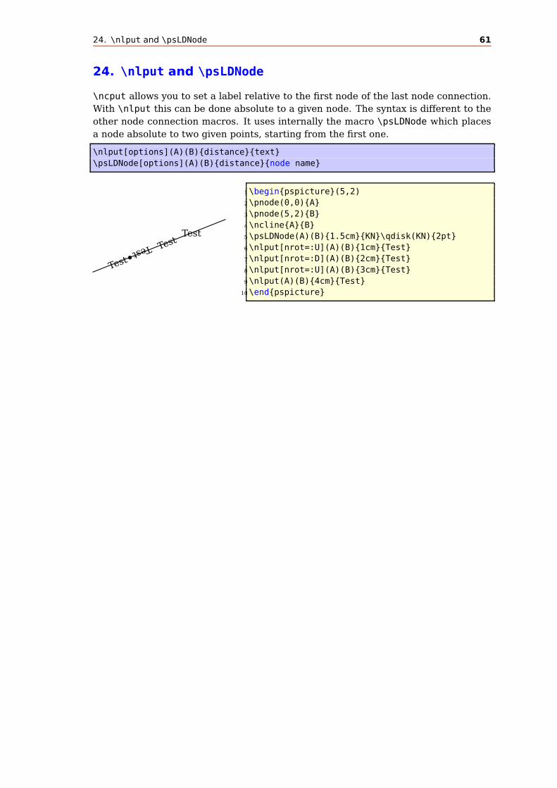
24. \nlput and \psLDNode 61
24. \nlput and \psLDNode
\ncput allows you to set a label relative to the first node of the last node connection.
With \nlput this can be done absolute to a given node. The syntax is different to the
other node connection macros. It uses internally the macro \psLDNode which places
a node absolute to two given points, starting from the first one.
\nlput[options](A)(B){distance}{text}
\psLDNode[options](A)(B){distance}{node name}
Test
Test TestTest
1\begin{pspicture}(5,2)
2\pnode(0,0){A}
3\pnode(5,2){B}
4\ncline{A}{B}
5\psLDNode(A)(B){1.5cm}{KN}\qdisk(KN){2pt}
6\nlput[nrot=:U](A)(B){1cm}{Test}
7\nlput[nrot=:D](A)(B){2cm}{Test}
8\nlput[nrot=:U](A)(B){3cm}{Test}
9\nlput(A)(B){4cm}{Test}
10\end{pspicture}

25. New syntax 62
Part III.
pst-plot
25. New syntax
There is now a new optional argument for \psplot and \parametricplot to pass
additional PostScript commands into the code. This makes the use of \pstVerb in
most cases superfluous.
\psplot [Options] {x0}{x1} [PS commands] {function}
\parametricplot [Options] {t0}{t1} [PS commands] {x(t) y(t)}
0
0.00075
0.00150
0.00225
0.00300
0 100 200 300 400 500 600 700 800 900 1000 1100
1\begin{pspicture}(0,-0.5)(12,5)
2 \psaxes[Dx=100,dx=1,Dy=0.00075,dy=1]{->}(0,0)(12,5)
3 \psplot[linecolor=red, plotstyle=curve,linewidth=2pt,plotpoints=200]{0}{11}%
4 [ /const1 3.3 10 8 neg exp mul def /s 10 def /const2 6.04 10 6 neg exp mul def ]%
5 { const1 x 100 mul dup mul mul Euler const2 neg x 100 mul dup mul mul exp mul 2000
mul}
6\end{pspicture}
26. New or extended options
The axes macro has now two additional optional arguments for placing labels at the
end of the axes:
\psaxes[settings]{arrows}(x0,y0)(x1,y1)(x2,y2)[Xlabel,Xangle][Ylabel,Yangle]
It has now four optional arguments, one for the setting, one for the arrows, one for
the x-label and one for the y-label. If you want only a y-label, then leave the x one
empty. A missing y-label is possible. The following examples show how it can be used.
The option tickstyle=full |top|bottom no longer works in the usual way. Only the
additional value inner is valid for pstricks-add, because everything can be set by the
ticksize option. When using the comma or trigLabels option, the macros \pshlabel
and \psvlabel shouldn’t be redefined, because the package does it itself internally
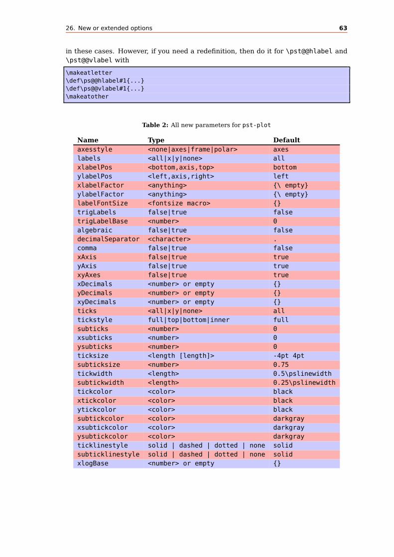
26. New or extended options 63
in these cases. However, if you need a redefinition, then do it for \pst@@hlabel and
\pst@@vlabel with
\makeatletter
\def\ps@@hlabel#1{...}
\def\ps@@vlabel#1{...}
\makeatother
Table 2: All new parameters for pst-plot
Name Type Default
axesstyle <none|axes|frame|polar> axes
labels <all|x|y|none> all
xlabelPos <bottom,axis,top> bottom
ylabelPos <left,axis,right> left
xlabelFactor <anything> {\ empty}
ylabelFactor <anything> {\ empty}
labelFontSize <fontsize macro> {}
trigLabels false|true false
trigLabelBase <number> 0
algebraic false|true false
decimalSeparator <character> .
comma false|true false
xAxis false|true true
yAxis false|true true
xyAxes false|true true
xDecimals <number> or empty {}
yDecimals <number> or empty {}
xyDecimals <number> or empty {}
ticks <all|x|y|none> all
tickstyle full|top|bottom|inner full
subticks <number> 0
xsubticks <number> 0
ysubticks <number> 0
ticksize <length [length]> -4pt 4pt
subticksize <number> 0.75
tickwidth <length> 0.5\pslinewidth
subtickwidth <length> 0.25\pslinewidth
tickcolor <color> black
xtickcolor <color> black
ytickcolor <color> black
subtickcolor <color> darkgray
xsubtickcolor <color> darkgray
ysubtickcolor <color> darkgray
ticklinestyle solid | dashed | dotted | none solid
subticklinestyle solid | dashed | dotted | none solid
xlogBase <number> or empty {}

26. New or extended options 64
Name Type Default
ylogBase <number> or empty {}
xylogBase <number> or empty {}
logLines <none|x|y|all> none
yMaxValue <real> -1
ignoreLines <number> 0
nStep <number> 1
nStart <number> 0
nEnd <number> or empty {}
xStep <number> 0
yStep <number> 0
xStart <number> or empty {}
yStart <number> or empty {}
xEnd <number> or empty {}
yEnd <number> or empty {}
plotNo <number> 1
plotNoMax <number> 1
xAxisLabel <anything> {\ empty}
yAxisLabel <anything> {\ empty}
xAxisLabelPos <(x,y)> or empty {\ empty}
yAxisLabelPos <(x,y)> or empty {\ empty}
llx <length> 0pt
lly <length> 0pt
urx <length> 0pt
ury <length> 0pt
polarplot false|true false
ChangeOrder false|true false

26.1. axesstyle 65
26.1. axesstyle
There is a new axes style polar which plots a polar coordinate system.
Syntax:
\psplot[axesstyle=polar](Rx,Ry)
\psplot[axesstyle=polar](...)(Rx,Ry)
\psplot[axesstyle=polar](...)(...)(Rx,Ry)
Important is the fact, that only one pair of coordinates is taken into account for the
radius. It is always the last pair in a sequence of allowed coordinates for the \psaxes
macro. The other ones are ignored; they are not valid for the polar coordinate system.
0
0
1
1
2
2
30
6090
120
150
180
210
240270
300
330
3600
0
1
1
2
2
30
60
90
120
150
180
210
240
270
300
330
360
1%\usepackage{pstricks-add}
2
3\begin{pspicture}(-3.5,-3.5)(3.5,3.5)
4\psaxes[axesstyle=polar](3,3)
5\psplot[polarplot,algebraic,linecolor=blue,linewidth=2pt,
6 plotpoints=2000]{0}{TwoPi 4 mul}{2*(sin(x)-x)/(cos(x)+x)}
7\end{pspicture}
8%
9\begin{pspicture}(-3.5,-3.5)(3.5,3.5)
10\psaxes[axesstyle=polar,subticklinestyle=dashed,subticks=2,
11 labelFontSize=\scriptstyle](3,3)
12\psplot[polarplot,algebraic,linecolor=red,linewidth=2pt,
13 plotpoints=2000]{0}{TwoPi}{6*sin(x)*cos(x)}
14\end{pspicture}
All valid optional arguments for the axes are also possible for the polar style, if
they make sense . . . :-) Important are the Dy option, it defines the angle interval and
subticks, for the intermediate circles and lines. The number can be different for the
circles (ysubticks) and the lines (xsubticks).

26.2. xyAxes, xAxis and yAxis 66
26.2. xyAxes, xAxis and yAxis
Syntax:
xyAxes=true|false
xAxis=true|false
yAxis=true|false
Sometimes there is only a need for one axis with ticks. In this case you can set
one of the preceding options to false. The xyAxes only makes sense when you want
to set both x and y to true with only one command, back to the default, because with
xyAxes=falseyou get nothing with the \psaxes macro.
0 1 2 3 4 0
1
2
3
4
0
1
2
3
4
0 1 2 3 4
1\begin{pspicture}(5,1)
2\psaxes[yAxis=false,linecolor=blue
]{->}(0,0.5)(5,0.5)
3\end{pspicture}
4\begin{pspicture}(1,5)
5\psaxes[xAxis=false,linecolor=red
]{->}(0.5,0)(0.5,5)
6\end{pspicture}
7\begin{pspicture}(1,5)
8\psaxes[xAxis=false,linecolor=red,
9 ylabelPos=right]{->}(0.5,0)
(0.5,5)
10\end{pspicture}\\[0.5cm]
11\begin{pspicture}(5,1)
12\psaxes[yAxis=false,linecolor=blue
,
13 xlabelPos=top]{->}(0,0.5)
(5,0.5)
14\end{pspicture}
As seen in the example, a single y axis gets the labels on the left side. This can be
changed with the option ylabelPos or with xlabelPos for the x-axis.
26.3. labels
Syntax:
labels=all|x|y|none
This option is also already in the pst-plot package and only mentioned here for
completeness.
1
−1
1−1
1\psset{ticksize=6pt}
2\begin{pspicture}(-1,-1)(2,2)
3\psaxes[labels=all,subticks=5]{->}(0,0)(-1,-1)(2,2)
4\end{pspicture}

26.4. xlabelPos and ylabelPos 67
1
−1
1\begin{pspicture}(-1,-1)(2,2)
2\psaxes[labels=y,subticks=5]{->}(0,0)(-1,-1)(2,2)
3\end{pspicture}
1 2
1\begin{pspicture}(-1,-1)(2,2)
2\psaxes[labels=x,subticks=5]{->}(0,0)(2,2)(-1,-1)
3\end{pspicture}
1\begin{pspicture}(-1,-1)(2,2)
2\psaxes[labels=none,subticks=5]{->}(0,0)(2,2)(-1,-1)
3\end{pspicture}
26.4. xlabelPos and ylabelPos
Syntax:
xlabelPos=bottom|axis|top
ylabelPos=left|axis|right
By default the labels for ticks are placed at the bottom (x axis) and left (y-axis). If
both axes are drawn in the negative direction the default is top (x axis) and right (y
axis). It be changed with the two options xlabelPos and ylabelPos. With the value
axis the user can place the labels depending on the value of labelsep, which is taken
into account for axis.
0
1
2
0 1 2
0
−1
−2
0 1 21\begin{pspicture}(3,3)
2\psaxes{->}(3,3)
3\end{pspicture}\hspace{2cm
}
4\begin{pspicture}(3,-3)
5\psaxes[xlabelPos=top
]{->}(3,-3)
6\end{pspicture}

26.5. Changing the label font size with labelFontSize and mathLabel 68
0
−1
−2
0−1−2
0
1
2
0 1 2
1\begin{pspicture}(-3,-3)
2\psaxes{->}(-3,-3)
3\end{pspicture}\hspace{2cm
}
4\begin{pspicture}(3,3)
5\psaxes[labelsep=0pt,
6 ylabelPos=axis,
7 xlabelPos=axis
]{->}(3,3)
8\end{pspicture}
0
−1
−2
0 1 2
1\begin{pspicture}(-1,1)(3,-3)
2\psaxes[xlabelPos=top,
3 xticksize=0 20pt,
4 yticksize=-20pt 0]{->}(3,-3)
5\end{pspicture}
26.5. Changing the label font size with labelFontSize and mathLabel
This option sets the horizontal and vertical font size for the labels depending on the
option mathLabel for the text or the math mode. It will be overwritten when another
package or a user defines
\def\pshlabel#1{\labelFontSize ...}
\def\psvlabel#1{\labelFontSize ...}
\def\pshlabel#1{$\labelFontSize ...$}% for mathLabel=true (default)
\def\psvlabel#1{$\labelFontSize ...$}% for mathLabel=true (default)
in another way. Note that for mathLabel=truethe font size must be set by one of the
mathematical styles \textstyle, \displaystyle, \scriptstyle, or \scriptscriptstyle.

26.6. xlabelFactor and ylabelFactor 69
0
1
2
0 1 2 3 4
x
y
0
1
2
0 1 2 3 4
0
1
2
0 1 2 3 4
1\psset{mathLabel=false}
2\begin{pspicture}(-0.25,-0.25)(5,2.25)
3\psaxes{->}(5,2.25)[$x$,0][$y$,90]
4\end{pspicture}\\[20pt]
5\begin{pspicture}(-0.25,-0.25)(5,2.25)
6\psaxes[labelFontSize=\footnotesize
]{->}(5,2.25)
7\end{pspicture}\\[20pt]
8\begin{pspicture}(-0.25,-0.25)(5,2.25)
9\psaxes[labelFontSize=\footnotesize
]{->}(5,2.25)
10\end{pspicture}\\[20pt]
0
1
2
0 1 2 3 4x
y
0
1
2
0 1 2 3 4
1\begin{pspicture}(-0.25,-0.25)(5,2.25)
2\psaxes[labelFontSize=\scriptstyle
]{->}(5,2.25)[\textbf{x},-90][\textbf{y
},0]
3\end{pspicture}\\[20pt]
4\psset{mathLabel=true}
5\begin{pspicture}(-0.25,-0.25)(5,2.25)
6\psaxes[labelFontSize=\scriptscriptstyle
]{->}(5,2.25)
7\end{pspicture}\\[20pt]
26.6. xlabelFactor and ylabelFactor
When having big numbers as data records then it makes sense to write the values as
< number > ·10<exp>. These new options allow you to define the additional part of the
value, but it must be set in math mode when using math operators!
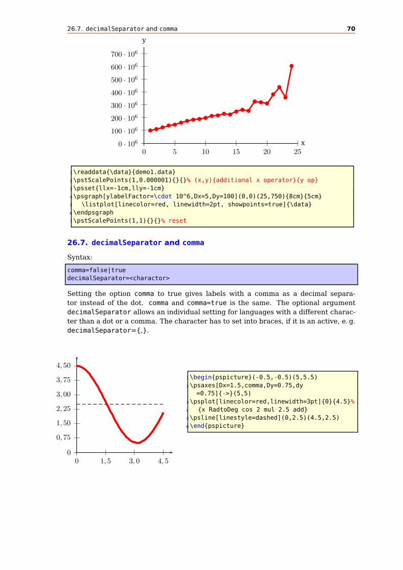
26.7. decimalSeparator and comma 70
0 · 106
100 · 106
200 · 106
300 · 106
400 · 106
500 · 106
600 · 106
700 · 106
0 5 10 15 20 25x
y
b b b b b b b b b b b b b b b b b
b b b
bb
b
b
1\readdata{\data}{demo1.data}
2\pstScalePoints(1,0.000001){}{}% (x,y){additional x operator}{y op}
3\psset{llx=-1cm,lly=-1cm}
4\psgraph[ylabelFactor=\cdot 10^6,Dx=5,Dy=100](0,0)(25,750){8cm}{5cm}
5 \listplot[linecolor=red, linewidth=2pt, showpoints=true]{\data}
6\endpsgraph
7\pstScalePoints(1,1){}{}% reset
26.7. decimalSeparator and comma
Syntax:
comma=false|true
decimalSeparator=<charactor>
Setting the option comma to true gives labels with a comma as a decimal separa-
tor instead of the dot. comma and comma=true is the same. The optional argument
decimalSeparator allows an individual setting for languages with a different charac-
ter than a dot or a comma. The character has to set into braces, if it is an active, e. g.
decimalSeparator={,}.
0
0, 75
1, 50
2, 25
3, 00
3, 75
4, 50
0 1, 5 3, 0 4, 5
1\begin{pspicture}(-0.5,-0.5)(5,5.5)
2\psaxes[Dx=1.5,comma,Dy=0.75,dy
=0.75]{->}(5,5)
3\psplot[linecolor=red,linewidth=3pt]{0}{4.5}%
4 {x RadtoDeg cos 2 mul 2.5 add}
5\psline[linestyle=dashed](0,2.5)(4.5,2.5)
6\end{pspicture}

26.8. xyDecimals, xDecimals and yDecimals 71
26.8. xyDecimals, xDecimals and yDecimals
Syntax:
xyDecimals=<number>
xDecimals=<any>
yDecimals=<any>
By default the labels of the axes get numbers with or without decimals, depending on
the numbers. With these options ??Decimals it is possible to determine the decimals,
where the option xyDecimals sets this identical for both axes. The default setting {}
means, that you’ll get the standard behaviour.
0.00
1.00
2.00
3.00
0.00 1.00 2.00 3.00 4.00
1\begin{pspicture}(-1.5,-0.5)(5,3.75)
2 \psaxes[xyDecimals=2]{->}(0,0)(4.5,3.5)
3\end{pspicture}
0,0
100,0
200,0
300,0
400,0
500,0
−100,0
0,250 0,500 0,750 1,000 1,250 Ampère
Voltage
1\psset{xunit=10cm,yunit=0.01cm,labelFontSize=\scriptstyle}
2\begin{pspicture}(-0.1,-150)(1.5,550.0)
3 \psaxes[Dx=0.25,Dy=100,ticksize=-4pt 0,comma=true,xDecimals=3,yDecimals
=1]{->}%
4 (0,0)(0,-100)(1.4,520)[\textbf{Amp\‘ere},-90][\textbf{Voltage},0]
5\end{pspicture}

26.9. trigLabels and trigLabelBase – axis with trigonmetrical units 72
26.9. trigLabels and trigLabelBase – axis with trigonmetrical units
With the option trigLabels=true the labels on the x axis are trigonometrical ones.
The option trigLabelBase set the denominator of fraction. The default value of 0 is
the same as no fraction. The following constants are defined in the package:
\def\psPiFour{12.566371}
\def\psPiTwo{6.283185}
\def\psPi{3.14159265}
\def\psPiH{1.570796327}
\newdimen\pstRadUnit
\newdimen\pstRadUnitInv
\pstRadUnit=1.047198cm % this is pi/3
\pstRadUnitInv=0.95493cm % this is 3/pi
Because it is a bit complicated to set the right values, we show some more examples
here.
For all following examples in this section we did a global
\psset{trigLabels=true,labelFontSize=\scriptstyle}.
Translating the decimal ticks to trigonometrical ones makes no real sense, because
every 1 xunit (1cm) is a tick and the last one is at 6cm.
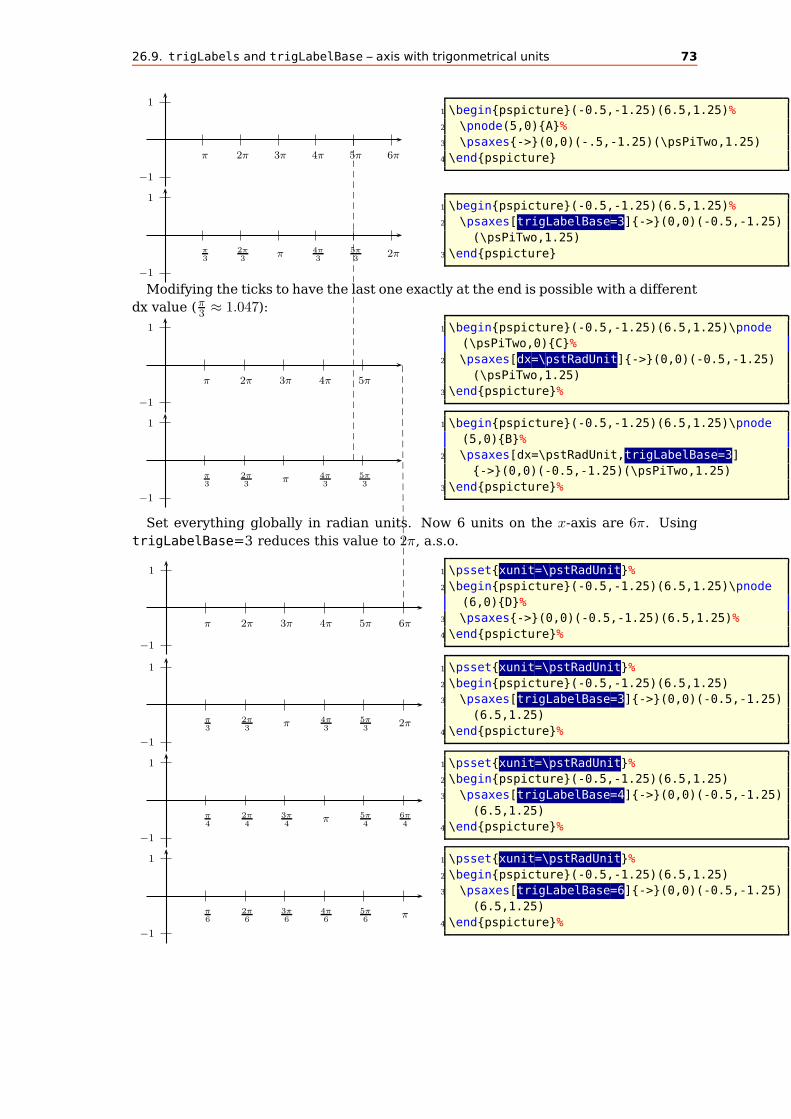
26.9. trigLabels and trigLabelBase – axis with trigonmetrical units 73
1
−1
π 2π 3π 4π 5π 6π
1 \begin{pspicture}(-0.5,-1.25)(6.5,1.25)%
2 \pnode(5,0){A}%
3 \psaxes{->}(0,0)(-.5,-1.25)(\psPiTwo,1.25)
4 \end{pspicture}
1
−1
π3
2π3
π 4π3
5π3
2π
1 \begin{pspicture}(-0.5,-1.25)(6.5,1.25)%
2 \psaxes[trigLabelBase=3]{->}(0,0)(-0.5,-1.25)
(\psPiTwo,1.25)
3 \end{pspicture}
Modifying the ticks to have the last one exactly at the end is possible with a different
dx value (π3 ≈ 1.047):
1
−1
π 2π 3π 4π 5π
1 \begin{pspicture}(-0.5,-1.25)(6.5,1.25)\pnode
(\psPiTwo,0){C}%
2 \psaxes[dx=\pstRadUnit]{->}(0,0)(-0.5,-1.25)
(\psPiTwo,1.25)
3 \end{pspicture}%
1
−1
π3
2π3
π 4π3
5π3
1 \begin{pspicture}(-0.5,-1.25)(6.5,1.25)\pnode
(5,0){B}%
2 \psaxes[dx=\pstRadUnit,trigLabelBase=3]
{->}(0,0)(-0.5,-1.25)(\psPiTwo,1.25)
3 \end{pspicture}%
Set everything globally in radian units. Now 6 units on the x-axis are 6π. Using
trigLabelBase=3 reduces this value to 2π, a.s.o.
1
−1
π 2π 3π 4π 5π 6π
1 \psset{xunit=\pstRadUnit}%
2 \begin{pspicture}(-0.5,-1.25)(6.5,1.25)\pnode
(6,0){D}%
3 \psaxes{->}(0,0)(-0.5,-1.25)(6.5,1.25)%
4 \end{pspicture}%
1
−1
π3
2π3
π 4π3
5π3
2π
1 \psset{xunit=\pstRadUnit}%
2 \begin{pspicture}(-0.5,-1.25)(6.5,1.25)
3 \psaxes[trigLabelBase=3]{->}(0,0)(-0.5,-1.25)
(6.5,1.25)
4 \end{pspicture}%
1
−1
π4
2π4
3π4
π 5π4
6π4
1 \psset{xunit=\pstRadUnit}%
2 \begin{pspicture}(-0.5,-1.25)(6.5,1.25)
3 \psaxes[trigLabelBase=4]{->}(0,0)(-0.5,-1.25)
(6.5,1.25)
4 \end{pspicture}%
1
−1
π6
2π6
3π6
4π6
5π6
π
1 \psset{xunit=\pstRadUnit}%
2 \begin{pspicture}(-0.5,-1.25)(6.5,1.25)
3 \psaxes[trigLabelBase=6]{->}(0,0)(-0.5,-1.25)
(6.5,1.25)
4 \end{pspicture}%

26.9. trigLabels and trigLabelBase – axis with trigonmetrical units 74
The best way seems to be to set the x-unit to \pstRadUnit. Plotting a function
doesn’t consider the value for trigLabelBase, it has to be done by the user. The first
example sets the unit locally for the \psplot back to 1cm, which is needed, because
we use this unit on the PostScript side.
1
−1
π3
2π3
π 4π3
5π3
2π
1 \psset{xunit=\pstRadUnit}%
2 \begin{pspicture}(-0.5,-1.25)(6.5,1.25)
3 \psaxes[trigLabelBase=3]{->}(0,0)(-0.5,-1.25)
(6.5,1.25)
4 \psplot[xunit=1cm,linecolor=red,linewidth=1.5
pt]{0}{\psPiTwo}{x RadtoDeg sin}
5 \end{pspicture}
1
−1
π3
2π3
π 4π3
5π3
2π
1 \psset{xunit=\pstRadUnit}%
2 \begin{pspicture}(-0.5,-1.25)(6.5,1.25)
3 \psaxes[trigLabelBase=3]{->}(0,0)(-0.5,-1.25)
(6.5,1.25)
4 \psplot[linecolor=red,linewidth=1.5pt]{0}{6}{
x Pi 3 div mul RadtoDeg sin}
5 \end{pspicture}
1
−1
π 2π 3π 4π
1 \psset{xunit=\pstRadUnit}%
2 \begin{pspicture}(-0.5,-1.25)(6.5,1.25)
3 \psaxes[dx=1.5]{->}(0,0)(-0.5,-1.25)
(6.5,1.25)
4 \psplot[xunit=0.5cm,linecolor=red,linewidth
=1.5pt]{0}{\psPiFour}{x RadtoDeg sin}
5 \end{pspicture}
1
−1
π2
π 3π2
2π 5π2
3π 7π2
4π
1 \psset{xunit=\pstRadUnit}%
2 \begin{pspicture}(-0.5,-1.25)(6.5,1.25)
3 \psaxes[dx=0.75,trigLabelBase=2]{->}(0,0)
(-0.5,-1.25)(6.5,1.25)
4 \psplot[xunit=0.5cm,linecolor=red,linewidth
=1.5pt]{0}{\psPiFour}{x RadtoDeg sin}
5 \end{pspicture}
It is also possible to set the x unit and dx value to get the labels right. But this
needs some more understanding as to how it really works. A xunit=1.570796327
sets the unit to π/2 and a dx=0.666667 then puts at every 2/3 of the unit a tick mark
and a label. The length of the x-axis is 6.4 units which is 6.4 · 1.570796327cm ≈ 10cm.
The function then is plotted from 0 to 3π = 9.424777961.
1
−1
π3
2π3
π 4π3
5π3
2π 7π3
8π3
3π
1 \begin{pspicture}(-0.5,-1.25)(10,1.25)
2 \psaxes[xunit=\psPiH,trigLabelBase=3,dx=0.666667]{->}(0,0)(-0.5,-1.25)
(6.4,1.25)
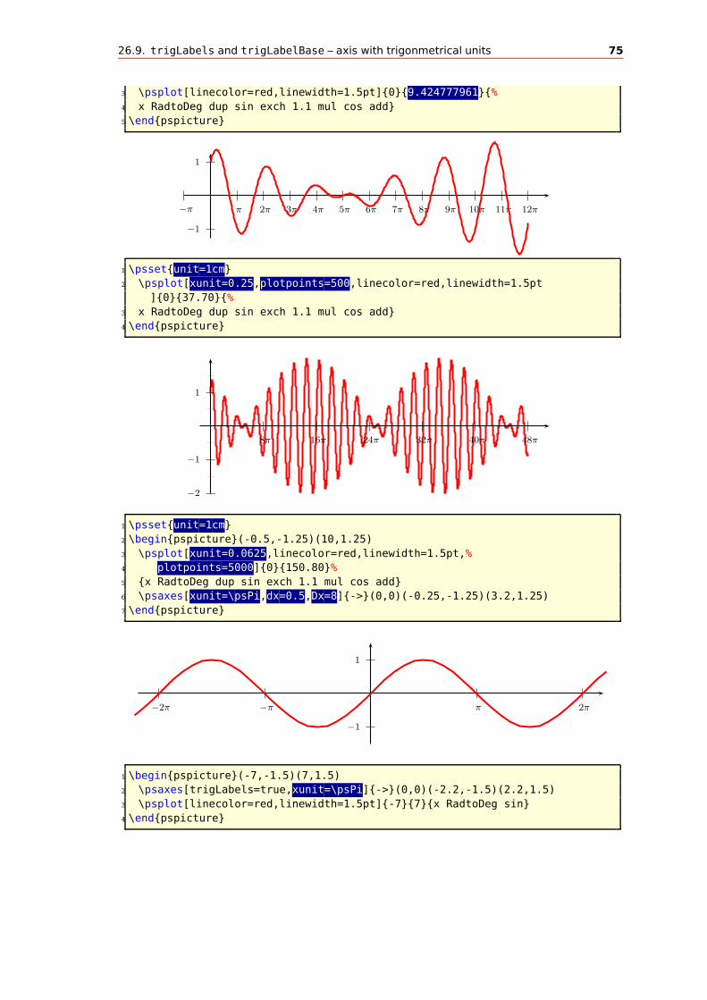
26.9. trigLabels and trigLabelBase – axis with trigonmetrical units 75
3 \psplot[linecolor=red,linewidth=1.5pt]{0}{9.424777961}{%
4 x RadtoDeg dup sin exch 1.1 mul cos add}
5 \end{pspicture}
1
−1
π 2π 3π 4π 5π 6π 7π 8π 9π 10π 11π 12π−π
1 \psset{unit=1cm}
2 \psplot[xunit=0.25,plotpoints=500,linecolor=red,linewidth=1.5pt
]{0}{37.70}{%
3 x RadtoDeg dup sin exch 1.1 mul cos add}
4 \end{pspicture}
1
−1
−2
8π 16π 24π 32π 40π 48π
1 \psset{unit=1cm}
2 \begin{pspicture}(-0.5,-1.25)(10,1.25)
3 \psplot[xunit=0.0625,linecolor=red,linewidth=1.5pt,%
4 plotpoints=5000]{0}{150.80}%
5 {x RadtoDeg dup sin exch 1.1 mul cos add}
6 \psaxes[xunit=\psPi,dx=0.5,Dx=8]{->}(0,0)(-0.25,-1.25)(3.2,1.25)
7 \end{pspicture}
1
−1
π 2π−π−2π
1 \begin{pspicture}(-7,-1.5)(7,1.5)
2 \psaxes[trigLabels=true,xunit=\psPi]{->}(0,0)(-2.2,-1.5)(2.2,1.5)
3 \psplot[linecolor=red,linewidth=1.5pt]{-7}{7}{x RadtoDeg sin}
4 \end{pspicture}

26.10. ticks 76
1
−1
π2
π 3π2
2π−π2
−π−3π2
−2π
1 \begin{pspicture}(-7,-1.5)(7,1.5)
2 \psaxes[trigLabels=true,
3 trigLabelBase=2,dx=\psPiH,xunit=\psPi]{->}(0,0)(-2.2,-1.5)(2.2,1.5)
4 \psplot[linecolor=red,linewidth=1.5pt]{-7}{7}{x RadtoDeg sin}
5 \end{pspicture}
26.10. ticks
Syntax:
ticks=all|x|y|none
This option is also already in the pst-plot package and only mentioned here for
some completeness.
1
−1
1−1
1\psset{ticksize=6pt}
2\begin{pspicture}(-1,-1)(2,2)
3\psaxes[ticks=all,subticks=5]{->}(0,0)(-1,-1)(2,2)
4\end{pspicture}
1
−1
1\begin{pspicture}(-1,-1)(2,2)
2\psaxes[ticks=y,subticks=5]{->}(0,0)(-1,-1)(2,2)
3\end{pspicture}
1 2
1\begin{pspicture}(-1,-1)(2,2)
2\psaxes[ticks=x,subticks=5]{->}(0,0)(2,2)(-1,-1)
3\end{pspicture}
1\begin{pspicture}(-1,-1)(2,2)
2\psaxes[ticks=none,subticks=5]{->}(0,0)(2,2)(-1,-1)
3\end{pspicture}
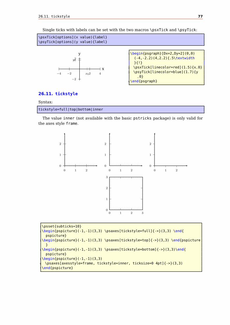
26.11. tickstyle 77
Single ticks with labels can be set with the two macros \psxTick and \psyTick:
\psxTick[options](x value){label}
\psyTick[options](y value){label}
2
−2
2 4−2−4
x
y
x0
y0
1\begin{psgraph}[Dx=2,Dy=2](0,0)
(-4,-2.2)(4,2.2){.5\textwidth
}{!}
2 \psxTick[linecolor=red](1.5){x_0}
3 \psyTick[linecolor=blue](1.7){y_0}
4\end{psgraph}
26.11. tickstyle
Syntax:
tickstyle=full|top|bottom|inner
The value inner (not available with the basic pstricks package) is only valid for
the axes style frame.
0
1
2
0 1 2
0
1
2
0 1 2
0
1
2
0 1 2
0
1
2
3
0 1 2 3
1\psset{subticks=10}
2\begin{pspicture}(-1,-1)(3,3) \psaxes[tickstyle=full]{->}(3,3) \end{
pspicture}
3\begin{pspicture}(-1,-1)(3,3) \psaxes[tickstyle=top]{->}(3,3) \end{pspicture
}
4\begin{pspicture}(-1,-1)(3,3) \psaxes[tickstyle=bottom]{->}(3,3)\end{
pspicture}
5\begin{pspicture}(-1,-1)(3,3)
6 \psaxes[axesstyle=frame, tickstyle=inner, ticksize=0 4pt]{->}(3,3)
7\end{pspicture}

26.12. ticksize, xticksize, yticksize 78
26.12. ticksize, xticksize, yticksize
With this new option the recent tickstyle option of pst-plot is obsolete and no
longer supported by pstricks-add.
Syntax:
ticksize=value[unit]
ticksize=value[unit] value[unit]
xticksize=value[unit]
xticksize=value[unit] value[unit]
yticksize=value[unit]
yticksize=value[unit] value[unit]
ticksize sets both values. The first one is left/below and the optional second one is
right/above of the coordinate axis. The old setting tickstyle=bottom is now easy to
realize, e.g.: ticksize=-6pt 0, or vice versa, if the coordinates are set from positive
to negative values.
1
2
3
−1
1 2 3−1
1\psset{arrowscale=2}
2\begin{pspicture}(-1.5,-1.5)(4,3.5)
3 \psaxes[ticksize=0.5cm]{->}(0,0)
(-1.5,-1.5)(4,3.5)
4\end{pspicture}
1
2
3
−1
1 2 3−1
1\psset{arrowscale=2}
2\begin{pspicture}(-1.5,-1.5)(4,3.5)
3 \psaxes[xticksize=-10pt 0,yticksize=0 10
pt]%
4 {->}(0,0)(-1.5,-1.5)(4,3.5)
5\end{pspicture}
A grid is also possible by setting the values to the max/min coordinates.

26.12. ticksize, xticksize, yticksize 79
1
2
3
4
1 2 3 4
1\psset{arrowscale=2}
2\begin{pspicture}(-.5,-.5)(5,4.5)
3 \psaxes[ticklinestyle=dashed,
4 ticksize=0 4cm]{->}(0,0)(-.5,-.5)
(5,4.5)
5\end{pspicture}

26.13. subticks 80
26.13. subticks
Syntax:
subticks=<number>
By default subticks cannot have labels.
1
−1
1−1
1\psset{ticksize=6pt}
2\begin{pspicture}(-1,-1)(2,2)
3\psaxes[ticks=all,subticks=5]{->}(0,0)(-1,-1)(2,2)
4\end{pspicture}
1
−1
1\begin{pspicture}(-1,-1)(2,2)
2\psaxes[ticks=y,subticks=5]{->}(0,0)(-1,-1)(2,2)
3\end{pspicture}
1 2
1\begin{pspicture}(-1,-1)(2,2)
2\psaxes[ticks=x,subticks=5]{->}(0,0)(2,2)(-1,-1)
3\end{pspicture}
1\begin{pspicture}(-1,-1)(2,2)
2\psaxes[ticks=none,subticks=5]{->}(0,0)(2,2)(-1,-1)
3\end{pspicture}
26.14. subticksize, xsubticksize, ysubticksize
Syntax:
subticksize=value
xsubticksize=value
ysubticksize=value
subticksize sets both values, which are relative to the ticksize length and can have
any number. 1 sets it to the same length as the main ticks.

26.15. tickcolor, subtickcolor 81
−1
−2
−3
−4
1 2 3−1
1\psset{yunit=1.5cm,xunit=3cm}
2\begin{pspicture}(-1.25,-4.75)(3.25,.75)
3 \psaxes[xticksize=-4.5 0.5,ticklinestyle=dashed,subticks=5,xsubticksize=1,
%
4 ysubticksize=0.75,xsubticklinestyle=dotted,xsubtickwidth=1pt,
5 subtickcolor=gray]{->}(0,0)(-1,-4)(3.25,0.5)
6\end{pspicture}
26.15. tickcolor, subtickcolor
Syntax:
tickcolor=<color>
xtickcolor=<color>
ytickcolor=<color>
subtickcolor=<color>
xsubtickcolor=<color>
ysubtickcolor=<color>
tickcolor and subtickcolor set both for the x- and the y-Axis.
0 1 2 3 4 5 6 7 8 9 10
1\begin{pspicture}(0,-0.75)(10,1)
2\psaxes[yAxis=false,labelFontSize=\scriptstyle,ticksize=0 10mm,subticks=10,
subticksize=0.75,
3 tickcolor=red,subtickcolor=blue,tickwidth=1pt,subtickwidth=0.5pt](10.01,0)
4\end{pspicture}

26.16. ticklinestyle and subticklinestyle 82
5 6 7 8 9 10
1\begin{pspicture}(5,-0.75)(10,1)
2\psaxes[yAxis=false,labelFontSize=\scriptstyle,
ticksize=0 -10mm,subticks=10,subticksize=0.75,
3 tickcolor=red,subtickcolor=blue,tickwidth=1pt,
subtickwidth=0.5pt,Ox=5](5,0)(5,0)(10.01,0)
4\end{pspicture}
26.16. ticklinestyle and subticklinestyle
Syntax:
ticklinestyle=solid|dashed|dotted|none
xticklinestyle=solid|dashed|dotted|none
yticklinestyle=solid|dashed|dotted|none
subticklinestyle=solid|dashed|dotted|none
xsubticklinestyle=solid|dashed|dotted|none
ysubticklinestyle=solid|dashed|dotted|none
ticklinestyle and subticklinestyle set both values for the x and y axis. The
value none doesn’t really makes sense, because it is the same as [sub]ticklines=0
100
101
0 1 2
1\psset{unit=4cm}
2\pspicture(-0.15,-0.15)(2.5,1)
3 \psaxes[axesstyle=frame,logLines=y,xticksize=0 1,xsubticksize=1,ylogBase
=10,
4 tickcolor=red,subtickcolor=blue,tickwidth=1pt,subticks=20,xsubticks=10,
5 xticklinestyle=dashed,xsubticklinestyle=dashed](2.5,1)
6\endpspicture
26.17. logLines
Syntax:
logLines=all|x|y
By default the option logLines sets the ticksize to the maximal length for x, y, or both.
It can be changed, when after the option logLines the ticksize is set.
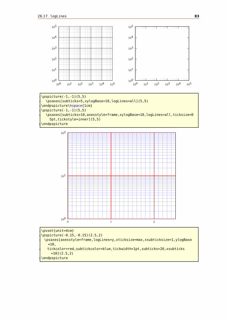
26.17. logLines 83
100
101
102
103
104
105
100 101 102 103 104 105100
101
102
103
104
105
100 101 102 103 104 105
1\pspicture(-1,-1)(5,5)
2 \psaxes[subticks=5,xylogBase=10,logLines=all](5,5)
3\endpspicture\hspace{1cm}
4\pspicture(-1,-1)(5,5)
5 \psaxes[subticks=10,axesstyle=frame,xylogBase=10,logLines=all,ticksize=0
5pt,tickstyle=inner](5,5)
6\endpspicture
100
101
102
0 1 2
1\psset{unit=4cm}
2\pspicture(-0.15,-0.15)(2.5,2)
3 \psaxes[axesstyle=frame,logLines=y,xticksize=max,xsubticksize=1,ylogBase
=10,
4 tickcolor=red,subtickcolor=blue,tickwidth=1pt,subticks=20,xsubticks
=10](2.5,2)
5\endpspicture

26.18. xylogBase, xlogBase and ylogBase 84
0
0.5
1.0
100 101 102 103
1\psset{unit=4}
2\pspicture(-0.5,-0.3)(3,1.2)
3 \psaxes[axesstyle=frame,tickstyle=inner,logLines=x,xlogBase=10,Dy=0.5,
tickcolor=red,
4 subtickcolor=blue,tickwidth=1pt,ysubticks=5,xsubticks=10](3,1)
5\endpspicture
26.18. xylogBase, xlogBase and ylogBase
There are additional options xylogBase, xlogBase, ylogBase to get one or both axes
with logarithmic labels. For an interval of [10−3...102] choose a pstricks interval of
[-3,2]. pstricks takes 0 as the origin of this axes, which is wrong if we want to have
a logarithmic axes. With the options Oy and Ox we can set the origin to −3, so that
the first label gets 10−3. If this is not done by the user then pstricks-add does it by
default. An alternative is to set these parameters to empty values Ox={},Oy={}, in
this case pstricks-add does nothing.
xylogBase
This mode in math is also called double logarithmic. It is a combination of the two
foregoing modes and the function is now y = log x and is shown in the following
example.

26.18. xylogBase, xlogBase and ylogBase 85
10-3
10-2
10-1
100
101
102
103
10-3 10-2 10-1 100 101 102 103x
y
y = log x
1\begin{pspicture}(-3.5,-3.5)(3.5,3.5)
2 \psplot[linewidth=2pt,linecolor=red
]{0.001}{3}{x log}
3 \psaxes[xylogBase=10,Oy=-3,Ox
=-3]{->}(-3,-3)(3.5,3.5)
4 \uput[-90](3.5,-3){x}
5 \uput[180](-3,3.5){y}
6 \rput(2.5,1){$y=\log x$}
7\end{pspicture}
ylogBase
The values for the \psaxes y-coordinate are now the exponents to the base 10 and for
the right function to the base e: 10−3 . . . 101 which corresponds to the given y-interval
−3 . . . 1.5, where only integers as exponents are possible. These logarithmic labels
have no effect on the internally used units. To draw the logarithm function we have
to use the math function
y = log{log x}y = ln{ln x}
with an drawing interval of 1.001 . . . 6.
10-3
10-2
10-1
100
101
0 1 2 3 4 5 6x
yy = log x
1\begin{pspicture}(-0.5,-3.5)(6.5,1.5)
2 \psaxes[ylogBase=10,Oy
=-3]{->}(0,-3)(6.5,1.5)
3 \uput[-90](6.5,-3){x}
4 \uput[0](0,1.4){y}
5 \rput(5,1){$y=\log x$}
6 \psplot[linewidth=2pt,%
7 plotpoints=100,linecolor=red
]{1.001}{6}{x log log} % log(log(x
))
8\end{pspicture}

26.18. xylogBase, xlogBase and ylogBase 86
e-3
e-2
e-1
e0
e1
0 1 2 3 4 5 6x
y
y = ln x1\begin{pspicture}(-0.5,-3.5)(6.5,1.5)
2 \psplot[linewidth=2pt,plotpoints
=100,linecolor=red]%
3 {1.04}{6}[ /ln {log 0.4343 div}
def ]{x ln ln} % log(x)
4 \psaxes[ylogBase=e,Oy=-3]{->}(0,-3)
(6.5,1.5)
5 \uput[-90](6.5,-3){x}
6 \uput[0](0,1.5){y}
7 \rput(5,1){$y=\ln x$}
8\end{pspicture}
102
103
104
0 1 2 3 4 5 6
1 \begin{pspicture}(-0.5,1.75)
(6.5,4.5)
2 \psaxes[ylogBase=10,Oy=2]{->}(0,2)
(0,2)(6.5,4.5)
3 \end{pspicture}
100
101
102
103
104
0 1 2 3 4 5 6
1 \begin{pspicture}(-0.5,-0.25)
(6.5,4.5)
2 \psplot{0}{6}{x x cos add log}
% x + cox(x)
3 \psplot[linecolor=red]{0}{6}{x 3
exp x cos add log} % x^3 + cos(x
)
4 \psplot[linecolor=cyan]{0}{6}{x 5
exp x cos add log} % x^5 + cos(x
)
5 \psaxes[ylogBase=10]{->}(6.5,4.5)
6 \end{pspicture}
100
101
102
103
104
105
0 1 2 3 4 5 6
1\begin{pspicture}(-0.5,-1.25)
(6.5,4.5)
2 \psplot{0}{6}{x x cos add log}
% x + cox(x)
3 \psplot[linecolor=red]{0}{6}{x 3
exp x cos add log} % x^3 + cos(x)
4 \psplot[linecolor=cyan]{0}{6}{x 5
exp x cos add log} % x^5 + cos(x)
5 \psaxes[ylogBase=10]{->}(0,-1)
(0,-1)(6.5,4.5)
6\end{pspicture}

26.18. xylogBase, xlogBase and ylogBase 87
102
103
104
3 4 5 6
1\begin{pspicture}(2.5,1.75)(6.5,4.5)
2 \psplot[linecolor=cyan]{3}{6}{x 5 exp x cos add log
} % x^5 + cos(x)
3 \psaxes[ylogBase=10,Ox=3,Oy=2]{->}(3,2)(3,2)
(6.5,4.5)
4\end{pspicture}
xlogBase
Now we have to use the easy math function y = x because the x axis is still log x.
−3
−2
−1
0
1
2
3
10-3 10-2 10-1 100 101 102 103x
y
y = log x
y = lnx
1\begin{pspicture}(-3.5,-3.5)(3.5,3.5)
2 \psplot[linewidth=2pt,linecolor=red
]{-3}{3}{x} % log(x)
3 \psplot[linewidth=2pt,linecolor=
blue]{-1.3}{1.5}{x 0.4343 div} %
ln(x)
4 \psaxes[xlogBase=10,Oy=-3,Ox
=-3]{->}(-3,-3)(3.5,3.5)
5 \uput[-90](3.5,-3){x}
6 \uput[180](-3,3.5){y}
7 \rput(2.5,1){$y=\log x$}
8 \rput[lb](0,-1){$y=\ln x$}
9\end{pspicture}
x
y
y = sin x
−1
0
1
10-1 100 101 102 103 104
1 \psset{yunit=3cm,xunit=2cm}
2 \begin{pspicture}(-1.25,-1.25)(4.25,1.5)

26.18. xylogBase, xlogBase and ylogBase 88
3 \uput[-90](4.25,-1){x}
4 \uput[0](-1,1.25){y}
5 \rput(0,1){$y=\sin x$}
6 \psplot[linewidth=2pt,plotpoints=5000,linecolor=red]{-1}{3.5}{10 x exp sin
}
7 \psaxes[xlogBase=10,Ox=-1,Oy=-1]{->}(-1,-1)(4.25,1.25)
8 \psline[linestyle=dashed](-1,0)(4,0)
9 \psline[linestyle=dashed](!-1 1)(!90 log 1)(!90 log -1)
10 \psline[linestyle=dashed](!90 log 1)(!180 log 1)(!180 log -1)
11 \end{pspicture}
1
2
−1
−2
101 102 10310-110-210-3
1\begin{pspicture}(-3.5,-2.5)(3.5,2.5)
2 \psaxes[xlogBase=10]{->}(0,0)
(-3.5,-2.5)(3.5,2.5)
3 \psplot{-2.5}{2.5}{10 x exp log}
4\end{pspicture}
1
2
−1
−2
101 102 10310-110-210-3
1\begin{pspicture}(-3.5,-2.5)(3.5,2.5)
2 \psaxes[xlogBase=10,Ox={},Oy
={}]{->}(0,0)(-3.5,-2.5)(3.5,2.5)
3 \psplot{-2.5}{2.5}{10 x exp log}
4\end{pspicture}
No logstyle (xylogBase={})
This is only a demonstration that the default option ={} still works ... :-)
1
2
0 1 2 3−1−2−3x
y
y = log x
1\begin{pspicture}(-3.5,-0.5)(3.5,2.5)
2 \psplot[linewidth=2pt,linecolor=red
,xylogBase={}]{0.5}{3}{x log} %
log(x)
3 \psaxes{->}(0,0)(-3.5,0)(3.5,2.5)
4 \uput[-90](3.5,0){x}
5 \uput[180](0,2.5){y}
6 \rput(2.5,1){$y=\log x$}
7\end{pspicture}

26.19. subticks, tickwidth and subtickwidth 89
26.19. subticks, tickwidth and subtickwidth
0 1 2 3 40−1−2−3−4−5
0−1−2−3−4 0 1 2 3 4 5
0 1 2 3 40−1−2−3−4−5
0 1 2 3 40−1−2−3−4−5
0−1−2−3−4 0 1 2 3 4 5
0−1−2−3−4 0 1 2 3 4 5
0 1 2 3 40−1−2−3−4−5
0−1−2−3−4 0 1 2 3 4 5
0 1 2 3 40−1−2−3−4−5
0−1−2−3−4 0 1 2 3 4 5
1 \psset{arrowscale=3,arrows=-D>,yAxis=false}
2 \psaxes[subticks=8](0,0)(-5,-1)(5,1)\\[1cm]
3 \psaxes[subticks=4,ticksize=-4pt 0,xlabelPos=top](0,0)(5,1)(-5,-1)\\
4 \psaxes[subticks=4,ticksize=-10pt 0](0,0)(-5,-5)(5,5)\\[1cm]
5 \psaxes[subticks=10,ticksize=0 -10pt](0,0)(-5,-5)(5,5)\\[1cm]
6 \psaxes[subticks=4,ticksize=0 10pt,xlabelPos=bottom](0,0)(5,5)(-5,-5)\\[1cm]
7 \psaxes[subticks=4,ticksize=0 -10pt,xlabelPos=top](0,0)(5,5)(-5,-5)\\[0.25cm]
8 \psaxes[subticks=0](0,0)(-5,-5)(5,5)\\[1cm]
9 \psaxes[subticks=0,tickcolor=red,linecolor=blue,xlabelPos=top](0,0)(5,5)(-5,-5)\\
10 \psaxes[subticks=5,tickwidth=2pt,subtickwidth=1pt](0,0)(-5,-5)(5,5)\\[1cm]
11 \psaxes[subticks=0,tickcolor=red,xlabelPos=top](0,0)(5,5)(-5,-5)}

26.19. subticks, tickwidth and subtickwidth 90
0
1
2
3
4
−1
−2
−3
−4
−5
0
−1
−2
−3
−4
1
2
3
4
5
0
1
2
3
4
−1
−2
−3
−4
−5
0
1
2
3
4
−1
−2
−3
−4
−5
0
−1
−2
−3
−4
1
2
3
4
5
0
−1
−2
−3
−4
1
2
3
4
5
0
1
2
3
4
−1
−2
−3
−4
−5
0
−1
−2
−3
−4
1
2
3
4
5
0
1
2
3
4
−1
−2
−3
−4
−5
0
−1
−2
−3
−4
1
2
3
4
5
1 \psset{arrowscale=3,xAxis=false}
2 \psaxes[subticks=8]{->}(0,0)(-5,-5)(5,5)\hspace{2em}
3 \psaxes[subticks=4,ylabelPos=right,ylabelPos=left]{->}(0,0)(5,5)(-5,-5)\hspace{4em}
4 \psaxes[subticks=4,ticksize=0 4pt]{->}(0,0)(-5,-5)(5,5)\hspace{3em}
5 \psaxes[subticks=4,ticksize=-4pt 0]{->}(0,0)(-5,-5)(5,5)\hspace{1em}
6 \psaxes[subticks=4,ticksize=0 4pt,ylabelPos=right]{->}(0,0)(5,5)(-5,-5)\hspace{3em}
7 \psaxes[subticks=4,ticksize=-4pt 0,linecolor=red,ylabelPos=right]{->}(0,0)(5,5)(-5,-5)
\hspace{5em}
8 \psaxes[subticks=0]{->}(0,0)(-5,-5)(5,5)\hspace{1em}
9 \psaxes[subticks=0,tickcolor=red,linecolor=blue,ylabelPos=right]{->}(0,0)(5,5)(-5,-5)\
hspace{5em}
10 \psaxes[subticks=5,tickwidth=2pt,subtickwidth=1pt]{->}(0,0)(-5,-5)(5,5)\hspace{1em}
11 \psaxes[subticks=5,tickcolor=red,tickwidth=2pt,%
12 ticksize=10pt,subtickcolor=blue,subticksize=0.75,ylabelPos=right]{->}(0,0)(5,5)
(-5,-5)

26.19. subticks, tickwidth and subtickwidth 91
0
1
2
3
4
0 1 2 3 4 5
1\pspicture(5,5.5)
2\psaxes[subticks=4,ticksize=6pt,subticksize
=0.5,%
3 tickcolor=red,subtickcolor=blue]{->}(5.4,5)
4\endpspicture
0
1
2
3
4
0 1 2 3 4 5
1\pspicture(5,5.5)
2 \psaxes[subticks=5,ticksize=0 6pt,
subticksize=0.5]{->}(5.4,5)
3\endpspicture
0
1
2
3
4
0 1 2 3 4 5
1\pspicture(5,5.5)
2 \psaxes[subticks=5,ticksize=-6pt 0,
subticksize=0.5]{->}(5.4,5)
3\endpspicture

26.19. subticks, tickwidth and subtickwidth 92
−1
−2
1
2
3
−1−2 1 2 3
1\pspicture(-3,-3)(3,3.5)
2 \psaxes[subticks=5,ticksize=0 6pt,
subticksize=0.5]{->}(0,0)(3,3)
(-3,-3)
3\endpspicture
0
−1
−2
0−1−2
1\pspicture(0,0.5)(-3,-3)
2 \psaxes[subticks=5,ticksize=-6pt 0,
subticksize=0.5,linecolor=red
]{->}(-3,-3)
3\endpspicture
0
1
2
3
4
5
0 1 2 3 4 5
1\psset{axesstyle=frame}
2\pspicture(5,5.5)
3 \psaxes[subticks=4,tickcolor=red,
subtickcolor=blue](5,5)
4\endpspicture

26.19. subticks, tickwidth and subtickwidth 93
0
1
2
3
4
5
0 1 2 3 4 5
1\pspicture(5,5.5)
2 \psaxes[subticks=5,subticksize=1,
subtickcolor=lightgray](5,5)
3\endpspicture
0
1
2
3
4
5
0 1 2 3 4 5
1\pspicture(5,5.5)
2 \psaxes[subticks=2,subticksize=1,
subtickcolor=lightgray](5,5)
3\endpspicture
0
1
2
3
4
0 1 2 3
1\pspicture(3,4.5)
2 \psaxes[subticks=5,ticksize=-7pt 0](3,4)
3\endpspicture
0
−1
−2
−3
−4
0−1−2−3
1\pspicture(0,1)(-3,-4)
2 \psaxes[subticks=5](-3,-4)
3\endpspicture

26.19. subticks, tickwidth and subtickwidth 94
0
1
2
3
4
0 1 2 3
1\pspicture(3,4.5)
2 \psaxes[axesstyle=axes,subticks=5](3,4)
3\endpspicture
0
−1
−2
−3
−4
0−1−2−3
1\pspicture(0,1)(-3,-4)
2 \psaxes[axesstyle=axes,subticks=5,%
3 ticksize=0 10pt](-3,-4)
4\endpspicture
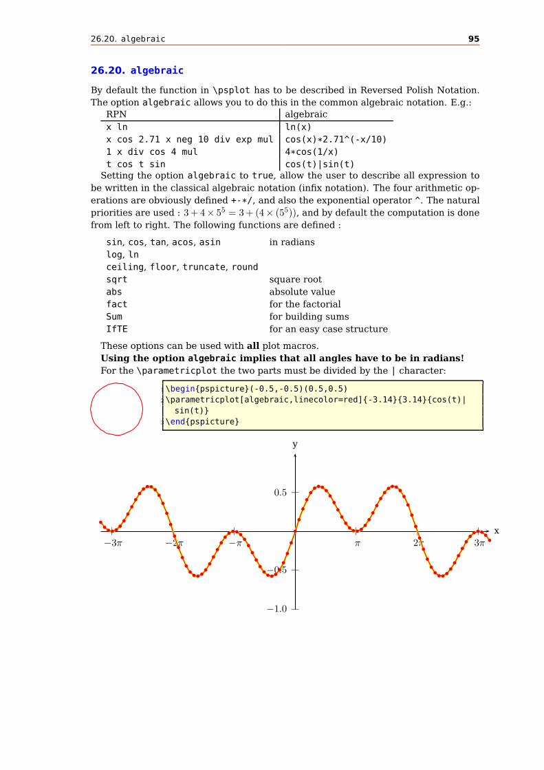
26.20. algebraic 95
26.20. algebraic
By default the function in \psplot has to be described in Reversed Polish Notation.
The option algebraic allows you to do this in the common algebraic notation. E.g.:
RPN algebraic
x ln ln(x)
x cos 2.71 x neg 10 div exp mul cos(x)*2.71^(-x/10)
1 x div cos 4 mul 4*cos(1/x)
t cos t sin cos(t)|sin(t)
Setting the option algebraic to true, allow the user to describe all expression to
be written in the classical algebraic notation (infix notation). The four arithmetic op-
erations are obviously defined +-*/, and also the exponential operator ^. The natural
priorities are used : 3 + 4 × 55 = 3 + (4 × (55)), and by default the computation is done
from left to right. The following functions are defined :
sin, cos, tan, acos, asin in radians
log, ln
ceiling, floor, truncate, round
sqrt square root
abs absolute value
fact for the factorial
Sum for building sums
IfTE for an easy case structure
These options can be used with all plot macros.
Using the option algebraic implies that all angles have to be in radians!
For the \parametricplot the two parts must be divided by the | character:
1\begin{pspicture}(-0.5,-0.5)(0.5,0.5)
2\parametricplot[algebraic,linecolor=red]{-3.14}{3.14}{cos(t)|
sin(t)}
3\end{pspicture}
0.5
−0.5
−1.0
π 2π 3π−π−2π−3πx
y
bbb b b
bb
b
b
b
bb b b b
b
b
b
b
b
b
b
bbb b b
bb
b
b
bbb b b b
b
b
b
b
bbb b b
b
b
b
b
b
b
b
b
bb b b
bb
b
b
b
bbb b b
bb
b
b
bbb b b b
b
b
b
b
b
b
b
bbb b b
b
b
b
b
bbb b b
bb

26.20. algebraic 96
1 \psset{lly=-0.5cm}
2 \psgraph[trigLabels,dx=\psPi,dy=0.5,Dy=0.5]{->}(0,0)(-10,-1)(10,1){\
linewidth}{6cm}
3 \psset{algebraic,plotpoints=1000}
4 \psplot[linecolor=yellow,linewidth=2pt]{-10}{10}{0.75*sin(x)*cos(x/2)}
5 \psplot[linecolor=red,showpoints=true,plotpoints=101]{-10}{10}{0.75*sin(x)
*cos(x/2)}
6 \endpsgraph
0
1
2
3
4
5
6
7
8
0 1 2 3 4 5 6 7 8 9 10 11 12 13 14 15 16 17 18x
yb
b
b
b
b
b
b
bb b
b
b
b
b
b
bb b b
b
b
b
b
bb
b b bb
bb
bb
b b b bb
bb
bb
b b b b bb
bb b
1 \psset{lly=-0.5cm}
2 \psgraph(0,-5)(18,3){15cm}{5cm}
3 \psset{algebraic,plotpoints=501}
4 \psplot[linecolor=yellow, linewidth=4\pslinewidth]{0.01}{18}{ln(x)}
5 \psplot[linecolor=red]{0.01}{18}{ln(x)}
6 \psplot[linecolor=yellow,linewidth=4\pslinewidth]{0}{18}{3*cos(x)*2.71^(-x
/10)}
7 \psplot[linecolor=blue,showpoints=true,plotpoints=51]{0}{18}{3*cos(x)
*2.71^(-x/10)}
8 \endpsgraph
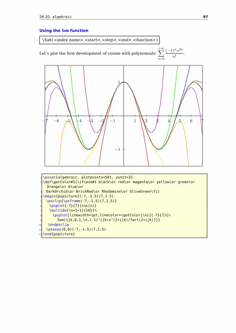
26.20. algebraic 97
Using the Sum function
\Sum(<index name>,<start>,<step>,<end>,<function>)
Let’s plot the first development of cosine with polynomials:
+∞∑
n=0
(−1)nx2n
n!.
1
−1
1 2 3 4 5 6 7−1−2−3−4−5−6−7
1 \psset{algebraic, plotpoints=501, yunit=3}
2 \def\getColor#1{\ifcase#1 black\or red\or magenta\or yellow\or green\or
Orange\or blue\or
3 DarkOrchid\or BrickRed\or Rhodamine\or OliveGreen\fi}
4 \begin{pspicture}(-7,-1.5)(7,1.5)
5 \psclip{\psframe(-7,-1.5)(7,1.5)}
6 \psplot{-7}{7}{cos(x)}
7 \multido{\n=1+1}{10}{%
8 \psplot[linewidth=1pt,linecolor=\getColor{\n}]{-7}{7}{%
9 Sum(ijk,0,1,\n,(-1)^ijk*x^(2*ijk)/fact(2*ijk))}}
10 \endpsclip
11 \psaxes(0,0)(-7,-1.5)(7,1.5)
12 \end{pspicture}

26.20. algebraic 98
Using the IfTE function
IfTE(<condition>,<true part>,<false part>)
Nesting of several IfTE is possible and seen in the following examples. A classic
example is a piece-wise linear function.
1
2
3
4
5
−1
−2
1 2 3 4 5 6 7−1−2−3−4−5−6−7x
y
1 \begin{pspicture}(-7.5,-2.5)(7.5,6)
2 \psaxes{->}(0,0)(-7,-2)(7.5,6)[x,-90][y,0]
3 \psset{algebraic=true, plotpoints=21,linewidth=2pt}
4 \psplot[linecolor=blue]{-7.5}{7.5}{IfTE(x<-6,8+x,IfTE(x<0,-x/3,IfTE(x<3,2*x,9-x)))}
5 \psplot[linecolor=red, plotpoints=101]{-7.5}{7.5}{%
6 IfTE(2*x<-2^2*sqrt(9),7+x,IfTE(x<0,x^2/18-1,IfTE(x<3,2*x^2/3-1,8-x)))}%
7 \end{pspicture}
When you program a piece-wise defined function you must take care that a plotting
point must be put at each point where the description changes. Use showpoints=true
to see what’s going on when there is a problem. You are on the safe side when you
choose a big number for plotpoints.

26.21. Plot style bar and option barwidth 99
1
2
3
4
5
6
7
−1
−2
−3
−4
−5
−6
−7
−8
1 2 3 4 5 6 7−1−2−3−4−5−6−7−8x
y
1 \psset{unit=0.75}
2 \begin{pspicture}(-8,-8)(8,8)
3 \psaxes{->}(0,0)(-8,-8)(8,8)[x,-90][y,0]
4 \psset{plotpoints=1000,linewidth=1pt}
5 \psplot[algebraic, linecolor=yellow]{-8}{8}{rand/(2^31-1)+x}
6 \psplot[algebraic]{-8}{8}{ceiling(x)}
7 \psplot[algebraic, linecolor=red]{-8}{8}{floor(x)}
8 \psplot[algebraic, linecolor=blue]{-8}{8}{round(x)}
9 \psplot[algebraic, linecolor=green]{-8}{8}{truncate(x)}
10 \psplot[algebraic, linecolor=cyan]{-8}{8}{div(mul(4,x),7)}
11 \psplot[algebraic, linecolor=gray]{-8}{8}{abs(x)+abs(x-3)-abs(5-5*x/7)}
12 \psplot[algebraic, linecolor=gray]{-8}{8}{abs(3*cos(x)+1)}
13 \psplot[algebraic, linecolor=magenta]{-8}{8}{floor(8*cos(x))}
14 \end{pspicture}
26.21. Plot style bar and option barwidth
This option allows you to draw bars for the data records. The width of the bars is
controlled by the option barwidth, which is set by default to value of 0.25cm, which
is the total width.

26.21. Plot style bar and option barwidth 100
0%
2%
4%
6%
8%
10%
12%
1466 1470 1474 1478 1482 1486 1490 1494
Amount
1\psset{xunit=.44cm,yunit=.3cm}
2\begin{pspicture}(-2,-3)(29,13)
3 \psaxes[axesstyle=axes,Ox=1466,Oy=0,Dx=4,Dy=2,xticksize=-6pt 0,
4 ylabelFactor={\,\%}]{-}(29,12)
5 \listplot[shadow=true,linecolor=blue,plotstyle=bar,barwidth=0.3cm,
6 fillcolor=red,fillstyle=solid]{\barData}
7 \rput{90}(-3,6.25){Amount}
8\end{pspicture}
0%
2%
4%
6%
8%
10%
12%
1466 1470 1474 1478 1482 1486 1490 1494
Amount
1\psset{xunit=.44cm,yunit=.3cm}
2\begin{pspicture}(-2,-3)(29,13)
3 \psaxes[axesstyle=axes,Ox=1466,Oy=0,Dx=4,Dy=2,ticksize=-4pt 0,
4 ylabelFactor={\,\%}]{-}(29,12)
5 \listplot[linecolor=blue,plotstyle=bar,barwidth=0.3cm,
6 fillcolor=red,fillstyle=crosshatch]{\barData}
7 \rput{90}(-3,6.25){Amount}
8\end{pspicture}

26.22. New options yMaxValue 101
0%
2%
4%
6%
8%
10%
12%
1466 1470 1474 1478 1482 1486 1490 1494
b b bb
b
b b
b
b
bb
b
b bb
bb b
b b bb
b
b
b bb
b
b
Amount
1\psset{xunit=.44cm,yunit=.3cm}
2\begin{pspicture}(-2,-3)(29,13)
3 \psaxes[axesstyle=axes,Ox=1466,Oy=0,Dx=4,Dy=2,ticksize=-4pt 0,
4 ylabelFactor={\,\%}]{-}(29,12)
5 \listplot[linecolor=blue,plotstyle=bar,barwidth=0.3cm,
6 fillcolor=red,fillstyle=vlines]{\barData}
7 \listplot[showpoints=true]{\barData}
8 \rput{90}(-3,6.25){Amount}
9\end{pspicture}
26.22. New options yMaxValue
With the new optional argument yMaxValue one can control the behaviour of discon-
tinued functions, like the tangent function. If yMaxValue is set to a negative value,
then the internal if clause is disabled, the function is plotted in the usual way as
known from pst-plot.

26.22. New options yMaxValue 102
1
2
3
4
5
6
−1
−2
−3
−4
−5
−6
π2 π 3π
2−π2−π−3π
2
x
y
×
1\begin{pspicture}(-6.5,-7)(6.5,7.5)
2\multido{\rA=-4.71239+\psPiH}{7}{%
3 \psline[linecolor=black!20,linestyle=dashed](\rA,-6.5)(\rA,6.5)}
4\psaxes[trigLabelBase=2,dx=\psPiH,
5 xunit=\psPi,trigLabels]{->}(0,0)(-1.7,-6.5)(1.77,6.5)[$x$,0][$y$,-90]
6\psset{algebraic,plotpoints=200,plotstyle=line}
7\psclip{\psframe[linestyle=none](-4.55,-6.5)(5.55,6.5)}
8 \psplot[yMaxValue=10,linewidth=1.6pt,linecolor=red]{-4.55}{4.55}{(x)/(sin
(2*x))}
9\endpsclip
10\psplot[linestyle=dashed,linecolor=blue!30]{-4.8}{4.8}{x}
11\psplot[linestyle=dashed,linecolor=blue!30]{-4.8}{4.8}{-x}
12\rput(0,0.5){$\times$}
13\end{pspicture}

26.22. New options yMaxValue 103
1
2
3
4
5
6
−1
−2
−3
−4
−5
−6
π2 π 3π
2−π2−π−3π
2
x
y
1\begin{pspicture}(-6.5,-7)(6.5,7.5)
2\psaxes[trigLabelBase=2,dx=\psPiH,
3 xunit=\psPi,trigLabels]{->}(0,0)(-1.7,-6.5)(1.77,6.5)[$x$,0][$y$,90]
4\psset{algebraic}
5\psplot[yMaxValue=6,linewidth=1.6pt,plotpoints=2000,
6 linecolor=red]{-4.55}{4.55}{tan(x)}
7\end{pspicture}

26.23. New options for \readdata 104
26.23. New options for \readdata
By default the macro \readdata reads every data record, which could be annoying
when you have some text lines at top of your data files or when there are more than
10000 records to read.
pstricks-add defines two additional keys ignoreLines and nStep, which allows
you to ignore preceding lines, e.g. ignoreLines=2, or to read only a selected part of
the data records, e.g. nStep=10, only every 10th record is saved.
1 \readdata[ignoreLines=2]{\dataA}{stressrawdata.data}
2 \readdata[nStep=10]{\dataA}{stressrawdata.data}
The default value for ignoreLines is 0 and for nStep is 1. the following data file has
two text lines which shall be ignored by the \readdata macro:
b
b
0
1
2
3
0 1
1\begin{filecontents*}{pstricks-add-data9.data}
2some nonsense in this line ---time forcex forcey
30 0.2
41 1
52 4
6\end{filecontents*}
7\readdata[ignoreLines=2]{\data}{pstricks-add-data9.
data}
8\pspicture(2,4)
9 \listplot[showpoints=true]{\data}
10 \psaxes{->}(2,4)
11\endpspicture
26.24. New options for \listplot
By default the plot macros \dataplot, \fileplot and \listplot plot every data
record. The package pst-plot-add defines additional keys nStep, nStart, nEnd, and
xStep, xStart, xEnd, which allows to plot only a selected part of the data records, e.g.
nStep=10. These "‘n"’ options mark the number of the record to be plot (0, 1, 2, ...) andthe "‘x"’ ones the x-values of the data records.
Name Default setting
nStart 1
nEnd {}
nStep 1
xStart {}
xEnd {}
yStart {}
yEnd {}
xStep 0
plotNo 1
plotNoMax 1
ChangeOrder false
(plotstyle) line
26.24. New options for \listplot 105
These new options are only available for the \listplot macro, which is not a real
limitation, because all data records can be read from a file with the \readdata macro
(see example files or [5]):
\readdata[nStep=10]{\data}{/home/voss/data/data1.data}
The use nStep and xStep options only make real sense when also using the op-
tion plotstyle=dots . Otherwise the coordinates are connected by a line as usual.
Also the xStep option needs increasing x values. Note that nStep can be used for
\readdata and for \listplot. If used in both macros then the effect is multiplied,
e.g. \readdata with nStep=5 and \listplot with nStep=10 means, that only every
50th data record is read and plotted.
When both, x/yStart/End are defined then the values are also compared with both
values.

26.24. New options for \listplot 106
Example for nStep/xStep
The datafile data.data contains 1000 data records. The thin blue line is the plot of all
records with the plotstyle option curve.
0 · 103
100 · 103
200 · 103
0 200 400 600 800 1000b b b b b b b b
bb
bb
bb
bb
bb
bb
1\readdata{\data}{data.data}
2\psset{xunit=12.5cm,yunit=0.2mm}
3\begin{pspicture}(-0.080,-30)(1,270)
4\pstScalePoints(1,1){1000 div}{1000 div}
5\psaxes[Dx=200,dx=2.5cm,Dy=100,ticksize=0 5pt,tickstyle=inner,
6 subticks=10,ylabelFactor=\cdot10^3,dy=2cm](0,0)(1,250)
7\listplot[nStep=50,linewidth=3pt,linecolor=red,plotstyle=dots]{\data}
8\listplot[linewidth=1pt,linecolor=blue]{\data}
9\end{pspicture}
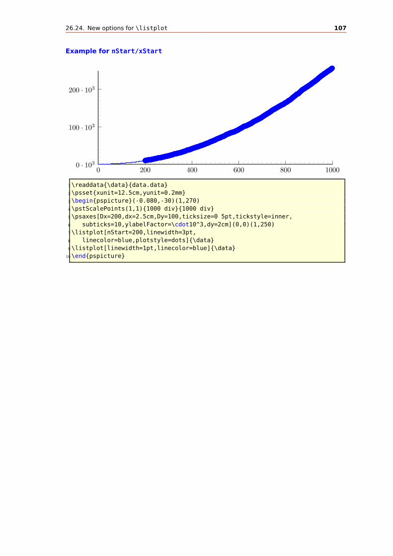
26.24. New options for \listplot 107
Example for nStart/xStart
0 · 103
100 · 103
200 · 103
0 200 400 600 800 1000
b b b b b b b b b b b b b b b b b b b b b b b b b b b b b b b b b b b b b b b b b b b b b b b b b b b b b b b b b b b b b b b b b b b b b b b b b b b b b b b b b b b bb b b b b b b b b b b b b b b b b b b b b b b b b b b b b b b b b b b b b b b b b b b b b b b b b b b b b b b b b b b b b b b b b b b
b b b b b b b b b b b b b b b b b b b b b b b b b b b b b b b b b b b b b b b b b b b b b b b b b bb b b b b b b b b b b b b b b b b b b b b b b b b b b b b b b b b b b b b b b b b b b b b b b b b
b b b b b b b b b b b b b b b b b b b b b b b b b b b b b b b b b b b b b b b b b bb b b b b b b b b b b b b b b b b b b b b b b b b b b b b b b b b b b b b b bb b b b b b b b b b b b b b b b b b b b b b b b b b b b b b b b b b b b bb b b b b b b b b b b b b b b b b b b b b b b b b b b b b b b b b b b b b bb b b b b b b b b b b b b b b b b b b b b b b b b b b b b b b b b b bb b b b b b b b b b b b b b b b b b b b b b b b b b b b b bb b b b b b b b b b b b b b b b b b b b b b b b b b b b b b bb b b b b b b b b b b b b b b b b b b b b b b b b b b bb b b b b b b b b b b b b b b b b b b b b b b b b b bb b b b b b b b b b b b b b b b b b b b b b b b b b b b b b b bb b b b b b b b b b b b b b b b b b b b b b b b b bb b b b b b b b b b b b b b b b b b b b b bb b b b b b b b b b b b b b b b b b b b b b bb b b b b b b b b b b b b b b b b b b b b bb b b b b b b b b b b b b b b b b b b b b b b b b bb b b b b b b b b b b b b b b b b b b b b bb b b b b b b b b b b b b b b b b b b b bb b b b b b b b b b b b b b b b b b b b b b b bb b b b b b b b b b b b b b b b b b b b b b b b b
1\readdata{\data}{data.data}
2\psset{xunit=12.5cm,yunit=0.2mm}
3\begin{pspicture}(-0.080,-30)(1,270)
4\pstScalePoints(1,1){1000 div}{1000 div}
5\psaxes[Dx=200,dx=2.5cm,Dy=100,ticksize=0 5pt,tickstyle=inner,
6 subticks=10,ylabelFactor=\cdot10^3,dy=2cm](0,0)(1,250)
7\listplot[nStart=200,linewidth=3pt,
8 linecolor=blue,plotstyle=dots]{\data}
9\listplot[linewidth=1pt,linecolor=blue]{\data}
10\end{pspicture}

26.24. New options for \listplot 108
Example for nEnd/xEnd
0 · 103
100 · 103
200 · 103
0 200 400 600 800 1000
1\readdata{\data}{data.data}
2\psset{xunit=12.5cm,yunit=0.2mm}
3\begin{pspicture}(-0.080,-30)(1,270)
4\pstScalePoints(1,1){1000 div}{1000 div}
5\psaxes[axesstyle=frame,Dx=200,dx=2.5cm,Dy=100,ticksize=0 5pt,tickstyle=
inner,
6 subticks=10,ylabelFactor=\cdot10^3,dy=2cm](0,0)(1,250)
7\listplot[nStart=200,linewidth=3pt,
8 linecolor=blue]{\data}
9\listplot[linewidth=1pt,linecolor=blue]{\data}
10\end{pspicture}

26.24. New options for \listplot 109
Example for all new options
0 · 103
100 · 103
200 · 103
0 200 400 600 800 1000
b b b bb
bb
bb
bb
bb
1\readdata{\data}{data.data}
2\psset{xunit=12.5cm,yunit=0.2mm}
3\begin{pspicture}(-0.080,-30)(1,270)
4\pstScalePoints(1,1){1000 div}{1000 div}
5\psaxes[axesstyle=frame,Dx=200,dx=2.5cm,Dy=100,,ticksize=0 5pt,tickstyle=
inner,
6 ylabelFactor=\cdot10^3,dy=2cm](0,0)(1,250)
7\listplot[nStart=200, nEnd=800, nStep=50,
8 linewidth=3pt,linecolor=blue,plotstyle=dots]{\data}
9\end{pspicture}

26.24. New options for \listplot 110
Example for xStart
This example shows the use of the same plot with different units and different xStart
value. The blue curve is the original plot of the data records. To show the important
part of the curve there is another one plotted with a greater yunit and a start value
of xStart=0.35. This makes it possible to have a kind of zoom to the original graphic.
0
100
200
300
400
500
−100
0.25 0.50 0.75 1.00 1.25
t [s]
flow[m
l/s]
leak volume
closing volume
1 \psset{xunit=10cm, yunit=0.01cm}
2 \readdata{\data}{data3.data}
3 \begin{pspicture}(-0.1,-100)(1.5,700.0)
4 \psaxes[Dx=0.25,Dy=100,dy=100\psyunit,ticksize=-4pt 0,%
5 labelFontSize={\scriptstyle}]{->}(0,0)(0,-100)(1.4,520)
6 \uput[0](1.4,0){\textsf{t [s]}}
7 \rput(-0.125,200){\psrotateleft{\small flow [ml/s]}}
8 \listplot[linewidth=2pt, linecolor=blue]{\data}
9 \rput(0.4,300){
10 \pscustom[yunit=0.04cm, linewidth=1pt]{%
11 \listplot[xStart=0.355]{\data}
12 \psline(1,-2.57)(1,0)(0.355,0)
13 \fill[fillstyle=hlines,fillcolor=gray,hatchwidth=0.4pt,hatchsep=1.5pt,
hatchcolor=red]%
14 \psline[linewidth=0.5pt]{->}(0.7,0)(1.05,0)
15 }%
16 }
17 \psline[linewidth=.01]{->}(0.75,300)(0.4,20)
18 \psline[linewidth=.01]{->}(1,290)(1.1,440)
19 \rput(1.1,470){\footnotesize leak volume}
20 \psline[linewidth=.01]{->}(0.78,200)(1,100)
21 \rput[l](1.02,100){\footnotesize closing volume}
22 \end{pspicture}
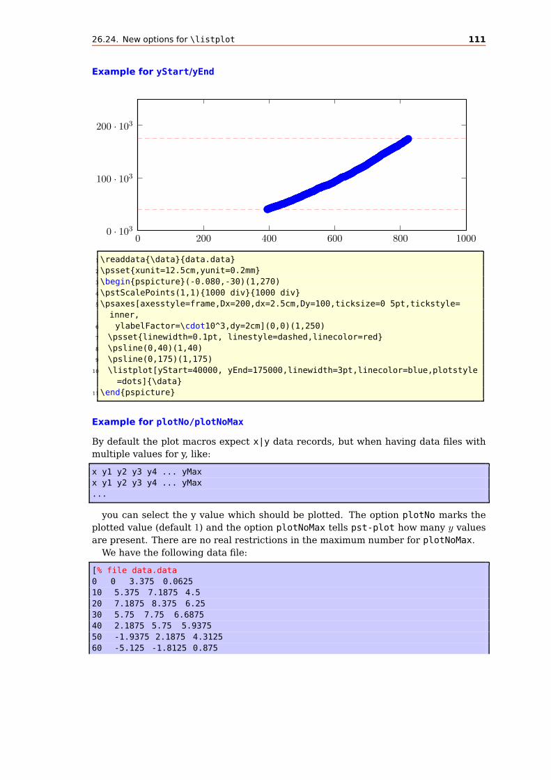
26.24. New options for \listplot 111
Example for yStart/yEnd
0 · 103
100 · 103
200 · 103
0 200 400 600 800 1000
b b b b b b b b b b b b b b b b b b b b b b b b b b b b b b b b b b b b b b b b b b b b b b b b b b bb b b b b b b b b b b b b b b b b b b b b b b b b b b b b b b b b b b b b b b b bb b b b b b b b b b b b b b b b b b b b b b b b b b b b b b b b b b b b b b bb b b b b b b b b b b b b b b b b b b b b b b b b b b b b b b b b b b b bb b b b b b b b b b b b b b b b b b b b b b b b b b b b b b b b b b b b b b b b bb b b b b b b b b b b b b b b b b b b b b b b b b b b b b b b b b bb b b b b b b b b b b b b b b b b b b b b b b b b b b b b bb b b b b b b b b b b b b b b b b b b b b b b b b b b b b b b bb b b b b b b b b b b b b b b b b b b b b b b b b b b bb b b b b b b b b b b b b b b b b b b b b b b b b bb b b b b b b b b b b b b b b b b b b b b b b b b b b b b bb b b b b b b b b b b b b b b b b b b b b b b b b b b b bb b b b b b b b b b b b b
1\readdata{\data}{data.data}
2\psset{xunit=12.5cm,yunit=0.2mm}
3\begin{pspicture}(-0.080,-30)(1,270)
4\pstScalePoints(1,1){1000 div}{1000 div}
5\psaxes[axesstyle=frame,Dx=200,dx=2.5cm,Dy=100,ticksize=0 5pt,tickstyle=
inner,
6 ylabelFactor=\cdot10^3,dy=2cm](0,0)(1,250)
7 \psset{linewidth=0.1pt, linestyle=dashed,linecolor=red}
8 \psline(0,40)(1,40)
9 \psline(0,175)(1,175)
10 \listplot[yStart=40000, yEnd=175000,linewidth=3pt,linecolor=blue,plotstyle
=dots]{\data}
11\end{pspicture}
Example for plotNo/plotNoMax
By default the plot macros expect x|y data records, but when having data files with
multiple values for y, like:
x y1 y2 y3 y4 ... yMax
x y1 y2 y3 y4 ... yMax
...
you can select the y value which should be plotted. The option plotNo marks the
plotted value (default 1) and the option plotNoMax tells pst-plot how many y values
are present. There are no real restrictions in the maximum number for plotNoMax.
We have the following data file:
[% file data.data
0 0 3.375 0.0625
10 5.375 7.1875 4.5
20 7.1875 8.375 6.25
30 5.75 7.75 6.6875
40 2.1875 5.75 5.9375
50 -1.9375 2.1875 4.3125
60 -5.125 -1.8125 0.875

26.24. New options for \listplot 112
70 -6.4375 -5.3125 -2.6875
80 -4.875 -7.1875 -4.875
90 0 -7.625 -5.625
100 5.5 -6.3125 -5.8125
110 6.8125 -2.75 -4.75
120 5.25 2.875 -0.75
]%
which holds data records for multiple plots (x y1 y2 y3). This can be plotted without
any modification to the data file:
0
2.5
5.0
−2.5
−5.0
−7.5
10 20 30 40 50 60 70 80 90 100 110 120 130 140x
y
1\readdata\Data{dataMul.data}
2\psset{xunit=0.1cm, yunit=0.5cm,lly=-0.5cm}
3\begin{pspicture}(0,-7.5)(150,10)
4\psaxes[Dx=10,Dy=2.5]{->}(0,0)(0,-7.5)(150,7.5)[$\mathbf{x}$,-90][$\mathbf{y
}$,0]
5\psset{linewidth=2pt,plotstyle=curve}
6\listplot[linecolor=green,plotNo=1,plotNoMax=3]{\Data}
7\listplot[linecolor=red,plotNo=2,plotNoMax=3]{\Data}
8\listplot[linecolor=blue,plotNo=3,plotNoMax=3]{\Data}
9\end{pspicture}

26.24. New options for \listplot 113
Example for changeOrder
It is only possible to fill the region between two listplots with \pscustom if one of
them has the values in reverse order. Otherwise we do not get a closed path. With
the option ChangeOrder the values are used in reverse order:
0
1
2
3
4
5
6
7
8
9
10
0 1 2 3 4 5 6 7 8 9 10x
y
1\begin{filecontents*}{test.data}
2 0 3 8
3 2 4 7
4 5 5 5.5
5 7 3.5 5
6 10 2 9
7\end{filecontents*}
8\psset{lly=-.5cm}
9\begin{psgraph}[axesstyle=frame,ticklinestyle=dotted,ticksize=0 10](0,0)
(10,10){4in}{2in}%
10 \readdata{\data}{test.data}%
11 \pscustom[fillstyle=solid,fillcolor=blue!40]{%
12 \listplot[plotNo=2,plotNoMax=2]{\data}%
13 \listplot[plotNo=1,plotNoMax=2,ChangeOrder]{\data}}
14\end{psgraph}

26.24. New options for \listplot 114
Example for plotstyle
The plotstyle option is defined in the package pst-plot, but its value LSM (Least
Square Method) is only valid for the pstricks-add package. Instead of plotting the
data records as dots or a line, the \listplot macro calculates the values for a line
y = v · x + u which fits best all data records.
0
1
2
3
4
5
6
7
0 1 2 3 4 5 6 7x
y
b
b
b
b
b
b
b
b
b
1 \begin{filecontents*}{LSM.data}
2 0 1 1 3 2.8 4 3 2.9 2 5 4 4 5 5.5 6 8.2 8 7
3 \end{filecontents*}
4 \psset{lly=-.5cm}
5 \readdata{\data}{LSM.data}
6 \begin{psgraph}[arrows=->](0,0)(0,0)(8,8){.5\textwidth}{!}
7 \listplot[plotstyle=dots]{\data}
8 \listplot[plotstyle=LSM,linecolor=red]{\data}
9 \end{psgraph}
The macro looks for the lowest and biggest x-value and draws the line for this
interval. It is possible to pass other values to the macro by setting the xStart and/or
xEnd options. They are preset with an empty value {}.

26.24. New options for \listplot 115
0
1
2
3
4
5
6
7
0 1 2 3 4 5 6 7x
y
b
b
b
b
b
b
b
b
b
y=0.755679 x+1.84105
1 \begin{filecontents*}{LSM.data}
2 0 1 1 3 2.8 4 3 2.9 2 5 4 4 5 5.5 6 8.2 8 7
3 \end{filecontents*}
4 \readdata{\data}{LSM.data}
5 \psset{lly=-1.75cm}
6 \begin{psgraph}[arrows=->](0,0)(0,0)(8,8){.5\textwidth}{!}
7 \listplot[plotstyle=dots]{\data}
8 \listplot[PstDebug=1,plotstyle=LSM,xStart=-0.5,xEnd=8.5,linecolor=red]{\
data}
9 \end{psgraph}
With PstDebug=1 one gets the equation y = v · x + u printed, beginning at the
position (0|-50pt). This cannot be changed, because it is only for some kind of de-
bugging. Pay attention for the correct xStart and xEnd values, when you use the
\pstScalePoints Macro. In the following example we use an x-interval from 0 to 3
to plot the values; first we subtract 0.003 from all x-values and then scale them with
10000. This is not taken into account for the xStart and xEnd values.

26.24. New options for \listplot 116
0
1
2
0.0030 0.0031 0.0032 0.0033x
y
b
b
b
b
y=-0.162184 x+2.27634
1 \begin{filecontents*}{LSM.data}
2 0.003298697 1.397785583
3 0.003193358 1.615489564
4 0.003094538 2.044019006
5 0.003001651 2.259240127
6 \end{filecontents*}
7 \readdata{\data}{LSM.data}
8 \pstScalePoints(10000,1){ 0.003 sub }{}
9 \psset{lly=-1.75cm}
10 \psgraph[arrows=->,Ox=0.0030,Dx=0.0001,dx=\psxunit](0,0)(3.2,3){10cm}{5cm}
11 \listplot[showpoints=true,linewidth=1pt,linecolor=blue]{\data}
12 \listplot[PstDebug=1,plotstyle=LSM,linewidth=0.1pt,linestyle=dashed,%
13 xStart=-0.25,xEnd=3.3]{\data}
14 \endpsgraph

27. Polar plots 117
27. Polar plots
With the option polarplot=false|true it is possible to use \psplot in polar mode:
\psplot [polarplot=true,...] {<start angle>}{<end angle>}%
[PS command] {<r(alpha)>}
The equation in PostScript code is interpreted as a function r = f(α), e.g. for the
circle with radius 1 as r =√
sin2 x + cos2 x, or r = a ∗ sin(x) ∗ cos(x)
(sin(x)3 + cos(x)3)for the
following examples:
x sin dup mul x cos dup mul add sqrt
1
2
3
4
−1
−2
−3
−4
1 2 3 4−1−2−3−4 x
y
0
1\psset{plotpoints=200,unit=0.75}
2\begin{pspicture*}(-5,-5)(5.1,5.1)
3 \psaxes[arrowlength=1.75,ticksize=2pt,labelFontSize=\scriptstyle,
4 linewidth=0.2mm]{->}(0,0)(-4.99,-4.99)(5,5)[x,-90][y,180]
5 \rput[Br](-.15,-.35){$0$} \psset{linewidth=.35mm,polarplot}
6 \psplot[linecolor=red]{140}{310}{3 neg x sin mul x cos mul x sin 3 exp x
cos 3 exp add div}
7 \psplot[linecolor=cyan]{140}{310}{6 x sin mul x cos mul x sin 3 exp x cos
3 exp add div}
8 \psplot[linecolor=blue,algebraic]{2.44}{5.41}{-8*sin(x)*cos(x)/(sin(x)^3+
cos(x)^3)}
9\end{pspicture*}

27. Polar plots 118
0
0
1
1
2
2
3
3
4
4
5
5
30
60
90
120
150
180
210
240
270
300
330
360
1\psset{unit=0.5cm}
2\begin{pspicture}(-6,-6)(6,6)
3\psaxes[axesstyle=polar,labelFontSize=\scriptstyle,linewidth=0.2mm]{->}(6,6)
4\psset{linewidth=3pt,polarplot,plotpoints=500,plotstyle=curve}
5\psclip{\pscircle[linestyle=none]{6}}
6 \psplot[linecolor=red]{140}{310}{3 neg x sin mul x cos mul x sin 3 exp x
cos 3 exp add div}
7 \psplot[linecolor=cyan]{140}{310}{6 x sin mul x cos mul x sin 3 exp x cos
3 exp add div}
8 \psplot[linecolor=blue,algebraic]{2.44}{5.41}{-8*sin(x)*cos(x)/(sin(x)^3+
cos(x)^3)}
9\endpsclip
10\end{pspicture}
1
2
−1
−2
1 2−1−2 x
y
0
1\psset{plotpoints=200,unit=1}
2\begin{pspicture}(-2.5,-2.5)(2.5,2.5)% Ulrich
Dirr
3 \psaxes[arrowlength=1.75,%
4 ticksize=2pt,linewidth=0.17mm]{->}%
5 (0,0)(-2.5,-2.5)(2.5,2.5)[$x$,-90][$y$,180]
6 \rput[Br](-.15,-.35){$0$}
7 \psset{linewidth=.35mm,plotstyle=curve,
polarplot=true}
8 \psplot[linecolor=red]{0}{360}{x cos 2 mul x
sin mul}
9 \psplot[linecolor=green]{0}{360}{x cos 3 mul x
sin mul}
10 \psplot[linecolor=blue]{0}{360}{x cos 4 mul x
sin mul}
11\end{pspicture}

27. Polar plots 119
2
4
6
8
−2
−4
−6
−8
2 4 6 8−2−4−6−8 x
y
0
1\psset{plotpoints=200,unit=0.5}
2\begin{pspicture}(-8.5,-8.5)
(9,9)% Ulrich Dirr
3\psaxes[Dx=2,dx=2,Dy=2,dy=2,
arrowlength=1.75,
4 ticksize=2pt,linewidth=0.17mm
]{->}(0,0)(-8.5,-8.5)(9,9)
5\rput[Br](9,-.7){$x$}
6\rput[tr](-.3,9){$y$}
7\rput[Br](-.3,-.7){$0$}
8%
9\psset{linewidth=.35mm,plotstyle
=curve,polarplot=true}
10\psplot[linecolor=blue
]{0}{720}{8 2.5 x mul sin mul}
11\end{pspicture}

28. \pstScalePoints 120
28. \pstScalePoints
The syntax is
\pstScalePoints(xScale,xScale){xPS}{yPS}
xScale,yScale are decimal values used as scaling factors, the xPs and yPS are addi-
tional PostScript code applied to the x- and y-values of the data records. This macro
is only valid for the \listplot macro!
0
1
2
3
4
5
0 1 2 3 4 5
b
b
b
b
b
b
b
b
b
b
b
b
b
b1\def\data{%
2 0 0 1 3 2 4 3 1
3 4 2 5 3 6 6 }
4\begin{pspicture}(-0.5,-1)(6,6)
5 \psaxes{->}(0,0)(6,6)
6 \listplot[showpoints=true,%
7 linecolor=red]{\data}
8 \pstScalePoints(1,0.5){}{3 add}
9 \listplot[showpoints=true,%
10 linecolor=blue]{\data}
11\end{pspicture}
\pstScalePoints(1,0.5){}{3 add} means that first the value 3 is added to the yvalues and second this value is scaled with the factor 0.5. As seen for the blue line
for x = 0 we get y(0) = (0 + 3) · 0.5 = 1.5.Changes with \pstScalePoints are always global to all following \listplotmacros.
This is the reason why it is a good idea to reset the values at the end of the pspicture
environment.

29. psCancel environment 121
Part IV.
New commands and
environments
29. psCancel environment1
This macro works like the \cancel macro from the package of the same name but it
allows as argument any contents, not only letters but also a complex graphic.
\psCancel * [Options] {contents}
All optional arguments for lines and boxes are valid and can be used in the usual
way. The star option fills the underlying box rectangle with the linecolor. This can be
transparent if opacity is set to a value less than 1. This can be used in presentation
to strike out words, equations, and graphic objects. Lines can also be transparent
when the option strokeopacity is used.
A Tikz :-)
0 · 108
1 · 108
2 · 108
3 · 108
4 · 108
5 · 108
6 · 108
7 · 108
0 5 10 15 20 25x-Axis
y-Axis
b bb b b
b bb b b
b b b bb b b
b b b
bb
b
b
first line
second line
first line
second line
0 · 108
1 · 108
2 · 108
3 · 108
4 · 108
5 · 108
6 · 108
7 · 108
0 5 10 15 20 25x-Axis
y-Axis
b bb b b
b bb b b
b b b bb b b
b b b
bb
b
b
(xR
yR
)
= r
︸︷︷︸
Scaling
·(
sin γ − cos γcos γ sin γ
)
︸ ︷︷ ︸
Rotation
(xK
yK
)
+
(txty
)
︸ ︷︷ ︸
Translation
1 Thanks to by Stefano Baroni

29. psCancel environment 122
1 \psCancel{A} \psCancel[linecolor=red]{Tikz :-)} \quad
2 \psCancel[linecolor=blue,doubleline=true]{%
3 \readdata{\data}{demo1.data}
4 \psset{shift=*,xAxisLabel=x-Axis,yAxisLabel=y-Axis,llx=-13mm,lly=-7mm,
5 xAxisLabelPos={c,-1},yAxisLabelPos={-7,c}}
6 \pstScalePoints(1,0.00000001){}{}
7 \begin{psgraph}[axesstyle=frame,xticksize=0 7.5,yticksize=0 25,subticksize
=1,
8 ylabelFactor=\cdot 10^8,Dx=5,Dy=1,xsubticks=2](0,0)(25,7.5){5.5cm}{5cm}
9 \listplot[linecolor=red, linewidth=2pt, showpoints=true]{\data}
10 \end{psgraph}} \qquad% end of Cancel
11 \psCancel[linewidth=3pt,linecolor=red,
12 strokeopacity=0.5]{\tabular[b]{c}first line\\second line\endtabular}\quad
13 \psCancel*[linecolor=red!50,opacity=0.5]{\tabular[b]{c}first line\\second
line\endtabular}
14 \quad
15 \psCancel*[linecolor=blue!30,opacity=0.5]{%
16 \readdata{\data}{demo1.data}
17 \psset{shift=*,xAxisLabel=x-Axis,yAxisLabel=y-Axis,llx=-15mm,lly=-7mm,urx
=1mm,
18 xAxisLabelPos={c,-1},yAxisLabelPos={-7,c}}
19 \pstScalePoints(1,0.00000001){}{}
20 \begin{psgraph}[axesstyle=frame,xticksize=0 7.5,yticksize=0 25,subticksize
=1,
21 ylabelFactor=\cdot 10^8,Dx=5,Dy=1,xsubticks=2](0,0)(25,7.5){5.5cm}{5cm}
22 \listplot[linecolor=red, linewidth=2pt, showpoints=true]{\data}
23 \end{psgraph}} \quad% end of Cancel
24 \psCancel[linewidth=4pt,strokeopacity=0.5]{\parbox{8cm}{\[
25 \binom{x_R}{y_R} = \underbrace{r\vphantom{\binom{A}{B}}}_{\text{Scaling}}\
cdot
26 \underbrace{\begin{pmatrix}
27 \sin\gamma & -\cos\gamma \\
28 \cos \gamma & \sin \gamma \\
29 \end{pmatrix}}_{\text{Rotation}} \binom{x_K}{y_K} +
30 \underbrace{\binom{t_x}{t_y}}_{\text{Translation}} \]} }% end of psCancel

30. psgraph environment 123
30. psgraph environment
This new environment psgraph does the scaling, it expects as parameter the values
(without units!) for the coordinate system and the values of the physical width and
height (with units!). The syntax is:
\psgraph [Options] {<arrows>}%
(xOrig,yOrig)(xMin,yMin)(xMax,yMax){xLength}{yLength}
. . .
\endpsgraph
\begin{psgraph} [Options] {<arrows>}%
(xOrig,yOrig)(xMin,yMin)(xMax,yMax){xLength}{yLength}
. . .
\end{psgraph}
where the options are valid only for the the \psaxes macro. The first two arguments
have the usual PSTricks behaviour.
• if (xOrig,yOrig) is missing, it is substituted to (xMin,xMax);
• if (xOrig,yOrig) and (xMin,yMin) are missing, they are both substituted to
(0,0).
The y-length maybe given as !, when the macro uses the same unit as for the x-axis.
0 · 106
100 · 106
200 · 106
300 · 106
400 · 106
500 · 106
600 · 106
700 · 106
0 5 10 15 20 25x
y
b b b b b b b b b b b b b bb b b
b b b
b
b
b
b
1 \readdata{\data}{demo1.data}
2 \pstScalePoints(1,0.000001){}{}% (x,y){additional x operator}{y op}
3 \psset{llx=-1cm,lly=-1cm}
4 \begin{psgraph}[axesstyle=frame,xticksize=0 759,yticksize=0 25,%
5 subticks=0,ylabelFactor=\cdot 10^6,
6 Dx=5,dy=100\psyunit,Dy=100](0,0)(25,750){10cm}{6cm} % parameters
7 \listplot[linecolor=red,linewidth=2pt,showpoints=true]{\data}
8 \end{psgraph}

30. psgraph environment 124
In the following example, the y unit gets the same value as the one for the x-axis.
0
1
2
3
0 1 2 3 4 5x
y
1 \psset{llx=-1cm,lly=-0.5cm,ury=0.5cm}
2 \begin{psgraph}(0,0)(5,3){6cm}{!} % x-y-axis with same unit
3 \psplot[linecolor=red,linewidth=1pt]{0}{5}{x dup mul 10 div}
4 \end{psgraph}
0 · 108
1 · 108
2 · 108
3 · 108
4 · 108
5 · 108
6 · 108
7 · 108
0 5 10 15 20 25x-Axis
y-Axis
b bb b b
b bb b b
b b b bb b b
b b b
bb
b
b
1 \readdata{\data}{demo1.data}
2 \psset{xAxisLabel=x-Axis,yAxisLabel=y-Axis,llx=-.5cm,lly=-1cm,ury=0.5cm,
3 xAxisLabelPos={c,-1},yAxisLabelPos={-7,c}}
4 \pstScalePoints(1,0.00000001){}{}
5 \begin{psgraph}[axesstyle=frame,xticksize=0 7.5,yticksize=0 25,subticksize
=1,
6 ylabelFactor=\cdot 10^8,Dx=5,Dy=1,xsubticks=2](0,0)(25,7.5){5.5cm}{5cm}
7 \listplot[linecolor=red, linewidth=2pt, showpoints=true]{\data}
8 \end{psgraph}

30. psgraph environment 125
0
200
400
600
0 5 10 15 20
x
y
b bb b b
b bb b b
b b b bb b b
b b b
bb
b
b
1\readdata{\data}{demo1.data}
2\psset{llx=-0.5cm,lly=-1cm}
3\pstScalePoints(1,0.000001){}{}
4\psgraph[arrows=->,Dx=5,dy=200\psyunit,Dy=200,subticks=5,ticksize=-10pt 0,
5 tickwidth=0.5pt,subtickwidth=0.1pt](0,0)(25,750){5.5cm}{5cm}
6\listplot[linecolor=red,linewidth=2pt,showpoints=true,plotstyle=LineToYAxis
]{\data}
7\endpsgraph
100
101
102
0 5 10 15 20 25x
y
b b b b b b b b b b b b b b b b b b b b b b b b
1 \readdata{\data}{demo1.data}
2 \pstScalePoints(1,0.2){}{log}
3 \psset{lly=-0.75cm}
4 \psgraph[ylogBase=10,Dx=5,Dy=1,subticks=5](0,0)(25,2){12cm}{4cm}
5 \listplot[linecolor=red, linewidth=2pt, showpoints=true]{\data}
6 \endpsgraph

30. psgraph environment 126
10-1
100
101
102
0 0.5 1.0 1.5 2.0 2.5x
y
b
bb
bb b b b b b b b b b b
b b b b b
1\readdata{\data}{demo0.data}
2\psset{lly=-0.75cm,ury=0.5cm}
3\pstScalePoints(1,1){}{log}
4\begin{psgraph}[arrows=->,Dx=0.5,ylogBase=10,Oy=-1,xsubticks=10,%
5 ysubticks=2](0,-3)(3,1){12cm}{4cm}
6 \listplot[linecolor=red,linewidth=2pt,showpoints=true,plotstyle=
LineToXAxis]{\data}
7\end{psgraph}
10-1
100
101
102
0 0.5 1.0 1.5 2.0 2.5x
y
b
bbb b
b bb b
b b bb b b
b bb b b
1\psset{lly=-0.75cm,ury=0.5cm}
2\readdata{\data}{demo0.data}
3\pstScalePoints(1,1){}{log}
4\psgraph[arrows=->,Dx=0.5,ylogBase=10,Oy=-1,subticks=4](0,-3)(3,1){6cm}{3cm}
5 \listplot[linecolor=red,linewidth=2pt,showpoints=true,plotstyle=
LineToXAxis]{\data}
6\endpsgraph

30. psgraph environment 127
0
1
2
3
4
5
6
1989 1991 1993 1995 1997 1999 2001
Year
Whatever
1 \readdata{\data}{demo2.data}%
2 \readdata{\dataII}{demo3.data}%
3 \pstScalePoints(1,1){1989 sub}{}
4 \psset{llx=-0.5cm,lly=-1cm, xAxisLabel=Year,yAxisLabel=Whatever,%
5 xAxisLabelPos={c,-0.4in},yAxisLabelPos={-0.4in,c}}
6 \psgraph[axesstyle=frame,Dx=2,Ox=1989,subticks=2](0,0)(12,6){4in}{2in}%
7 \listplot[linecolor=red,linewidth=2pt]{\data}
8 \listplot[linecolor=blue,linewidth=2pt]{\dataII}
9 \listplot[linecolor=cyan,linewidth=2pt,yunit=0.5]{\dataII}
10 \endpsgraph
2
3
4
5
6
1989 1991 1993 1995 1997 1999 2001x
y
1 \readdata{\data}{demo2.data}%
2 \readdata{\dataII}{demo3.data}%
3 \psset{llx=-0.5cm,lly=-0.75cm,plotstyle=LineToXAxis}

30.1. The new options 128
4 \pstScalePoints(1,1){1989 sub}{2 sub}
5 \begin{psgraph}[axesstyle=frame,Dx=2,Ox=1989,Oy=2,subticks=2](0,0)(12,4){6in
}{3in}
6 \listplot[linecolor=red,linewidth=12pt]{\data}
7 \listplot[linecolor=blue,linewidth=12pt]{\dataII}
8 \listplot[linecolor=cyan,linewidth=12pt,yunit=0.5]{\dataII}
9 \end{psgraph}
An example with ticks on every side of the frame and filled areas:
x
y
0
2
4
6
8
0 1 2 3
level 1
level 2
1 \def\data{0 0 1 4 1.5 1.75 2.25 4 2.75 7 3 9}
2 \psset{lly=-0.5cm}
3 \begin{psgraph}[axesstyle=none,ticks=none](0,0)(3.0,9.0){12cm}{5cm}
4 \pscustom[fillstyle=solid,fillcolor=red!40,linestyle=none]{%
5 \listplot{\data}
6 \psline(3,9)(3,0)}
7 \pscustom[fillstyle=solid,fillcolor=blue!40,linestyle=none]{%
8 \listplot{\data}
9 \psline(3,9)(0,9)}
10 \listplot[linewidth=2pt]{\data}
11 \psaxes[axesstyle=frame,ticksize=0 5pt,xsubticks=20,ysubticks=4,
12 tickstyle=inner,dy=2,Dy=2,tickwidth=1.5pt,subtickcolor=black](0,0)(3,9)
13 \rput*(2.5,3){level 1}\rput*(1,7){level 2}
14 \end{psgraph}
30.1. The new options
name default meaning
xAxisLabel x label for the x-axis
yAxisLabel y label for the y-axis
xAxisLabelPos {} where to put the x-label
yAxisLabelPos {} where to put the y-label
llx 0pt trim for the lower left x
lly 0pt trim for the lower left y
urx 0pt trim for the upper right x
ury 0pt trim for the upper right y

30.2. Problems 129
There is one restriction in using the trim parameters, they must been set before
\psgraph is called. They are redundant when used as parameters of \psgraph itself.
The ?AxisLabelPos options can use the letter c for centering an x-axis or y-axis label.
The c is a replacement for the x or y value. When using values with units, the position
is always measured from the origin of the coordinate system, which can be outside
the visible pspicture environment
0
1
2
3
4
5
6
1989 1990 1991 1992 1993 1994 1995 1996 1997 1998 1999 2000 2001
Year
Whatever
1 \readdata{\data}{demo2.data}%
2 \readdata{\dataII}{demo3.data}%
3 \psset{llx=-1cm,lly=-1.25cm,urx=0.5cm,ury=0.1in,xAxisLabel=Year,%
4 yAxisLabel=Whatever,xAxisLabelPos={c,-0.4in},%
5 yAxisLabelPos={-0.4in,c}}
6 \pstScalePoints(1,1){1989 sub}{}
7 \psframebox[linestyle=dashed,boxsep=0pt]{%
8 \begin{psgraph}[axesstyle=frame,Ox=1989,subticks=2](0,0)(12,6){0.8\linewidth
}{2.5in}%
9 \listplot[linecolor=red,linewidth=2pt]{\data}%
10 \listplot[linecolor=blue,linewidth=2pt]{\dataII}%
11 \listplot[linecolor=cyan,linewidth=2pt,yunit=0.5]{\dataII}%
12 \end{psgraph}%
13 }
30.2. Problems
Floating point operations in TEX are a real mess, which causes a lot of problems when
there are very small or very big units. With the options of pst-plot it is possible to
choose normal units (whatever this may be ...), and plot the data as usual.

30.2. Problems 130
0
10
20
30
40
50
60
70
3.23 3.24 3.25 3.26x
y
b
b
b
1\begin{filecontents*}{test.data}
23.2345 34.5
33.2364 65.4
43.2438 50.2
5\end{filecontents*}
6
7\psset{lly=-0.5cm,llx=-1cm}
8\readdata{\data}{test.data}
9\pstScalePoints(1,1){3.23 sub 100 mul}{}
10\begin{psgraph}[Ox=3.23,Dx=0.01,dx=\psxunit,Dy=10](0,0)(3,70){0.8\linewidth
}{5cm}%
11 \listplot[showpoints=true,plotstyle=curve]{\data}
12\end{psgraph}
This example shows some important facts:
• 3.23 sub 100 mul: the x values are now 0.45; 0.64; 1.38
• Ox=3.23: the origin of the x axis is set to 3.23
• Dx=0.01: the increment of the labels
• dx=\psxunit: uses the calculated unit value to get every unit a label
• Dy=10: increase the y labels by 10
Using the internal \psxunit one can have dynamical x-units, depending on the
linewidth of the document.

31. \psStep 131
31. \psStep
\psStep calculates a step function for the upper or lower sum or the max/min of the
Riemann integral definition of a given function. The available option is
StepType=lower |upper|Riemann|infimum|supremum or alternative StepType=l |u|R|i|s
with lower as the default setting. The syntax of the function is
\psStep [Options] (()x1,x2){n}{function}
(x1,x2) is the given interval for the step wise calculated function, n is the number
of the rectangles and function is the mathematical function in postfix or algebraic
notation (with algebraic=true ).
0
1
2
0 1 2 3 4 5 6 7 8 9
1\begin{pspicture}(-0.5,-0.5)(10,3)
2 \psaxes[labelFontSize=\scriptstyle]{->}(10,3)
3 \psplot[plotpoints=100,linewidth=1.5pt,algebraic]{0}{10}{sqrt(x)}
4 \psStep[linecolor=magenta,StepType=upper,fillstyle=hlines](0,9){9}{x sqrt}
5 \psStep[linecolor=blue,fillstyle=vlines](0,9){9}{x sqrt }
6\end{pspicture}
0
1
2
−1
−2
1 2 3 4 5 6 7 8 9
1\psset{plotpoints=200}
2\begin{pspicture}(-0.5,-2.25)(10,3)
3 \psaxes[labelFontSize=\scriptstyle]{->}(0,0)(0,-2.25)(10,3)
4 \psplot[linewidth=1.5pt,algebraic]{0}{10}{sqrt(x)*sin(x)}
5 \psStep[algebraic,linecolor=magenta,StepType=upper](0,9){20}{sqrt(x)*sin(x)
}
6 \psStep[linecolor=blue,linestyle=dashed](0,9){20}{x sqrt x RadtoDeg sin mul
}
7\end{pspicture}

31. \psStep 132
0
1
−1
1 2 3 4 5 6 7 8 9
1\psset{yunit=1.25cm,plotpoints=200}
2\begin{pspicture}(-0.5,-1.5)(10,1.5)
3 \psaxes[labelFontSize=\scriptstyle]{->}(0,0)(0,-1.5)(10,1.5)
4 \psStep[algebraic,StepType=Riemann,fillstyle=solid,fillcolor=black
!10](0,10){50}%
5 {sqrt(x)*cos(x)*sin(x)}
6 \psplot[linewidth=1.5pt,algebraic]{0}{10}{sqrt(x)*cos(x)*sin(x)}
7\end{pspicture}
0
1
−1
1 2 3 4 5 6 7 8 9
1\psset{yunit=1.25cm,plotpoints=200}
2\begin{pspicture}(-0.5,-1.5)(10,1.5)
3 \psaxes[labelFontSize=\scriptstyle]{->}(0,0)(0,-1.5)(10,1.5)
4 \psStep[algebraic,StepType=infimum,fillstyle=solid,fillcolor=black
!10](0,10){50}%
5 {sqrt(x)*cos(x)*sin(x)}
6 \psplot[linewidth=1.5pt,algebraic]{0}{10}{sqrt(x)*cos(x)*sin(x)}
7\end{pspicture}

31. \psStep 133
0
1
−1
1 2 3 4 5 6 7 8 9
1\psset{yunit=1.25cm,plotpoints=200}
2\begin{pspicture}(-0.5,-1.5)(10,1.5)
3 \psaxes[labelFontSize=\scriptstyle]{->}(0,0)(0,-1.5)(10,1.5)
4 \psStep[algebraic,StepType=supremum,fillstyle=solid,fillcolor=black
!10](0,10){50}%
5 {sqrt(x)*cos(x)*sin(x)}
6 \psplot[linewidth=1.5pt,algebraic]{0}{10}{sqrt(x)*cos(x)*sin(x)}
7\end{pspicture}
0
1
2
−1
−2
1 2 3 4 5 6 7 8 9
f(x) = 2 · √x · cos (ln x) · sin x
1\psset{unit=1.5cm,plotpoints=200}
2\begin{pspicture}[plotpoints=200](-0.5,-3)(10,2.5)
3 \psStep[algebraic,fillstyle=solid,fillcolor=yellow](0.001,9.5){40}{2*sqrt(
x)*cos(ln(x))*sin(x)}
4 \psStep[algebraic,StepType=Riemann,fillstyle=solid,fillcolor=blue
](0.001,9.5){40}{2*sqrt(x)*cos(ln(x))*sin(x)}
5 \psaxes[labelFontSize=\scriptstyle]{->}(0,0)(0,-2.75)(10,2.5)
6 \psplot[algebraic,linecolor=white]{0.001}{9.75}{2*sqrt(x)*cos(ln(x))*sin(x
)}
7 \uput[90](6,1.2){$f(x)=2\cdot\sqrt{x}\cdot\cos{(\ln{x})}\cdot\sin{x}$}
8\end{pspicture}

32. \psplotTangent and option Tnormal 134
32. \psplotTangent and option Tnormal
There is an additional option, named Derive for an alternative function (see following
example) to calculate the slope of the tangent. This will be in general the first deriva-
tive, but can also be any other function. If this option is different to to the default
value Derive=default , then this function is taken to calculate the slope. For the
other cases, pstricks-add builds a secant with -0.00005<x<0.00005, calculates the
slope and takes this for the tangent. This may be problematic in some cases of special
functions or x values, then it may be appropriate to use the Derive option.
\psplotTangent * [Options] {x}{dx}{function}
The macro expects three parameters:
x : the x value of the function for which the tangent should be calculated
dx : the dx to both sides of the x value
f(x) : the function in infix (with option algebraic) or the default postfix (PostScript)
notation
The following examples show the use of the algebraic option together with the
Derive option. Remember that using the algebraic option implies that the angles
have to be in the radian unit!
1
2
3
−1
−2
1 2 3 4 5 6 7−1−2−3−4−5−6−7
1 \def\F{x RadtoDeg dup dup cos exch 2 mul cos add exch 3 mul cos add}
2 \def\Fp{x RadtoDeg dup dup sin exch 2 mul sin 2 mul add exch 3 mul sin 3 mul
add neg}
3 \psset{plotpoints=1001}
4 \begin{pspicture}(-7.5,-2.5)(7.5,4)%X\psgrid
5 \psaxes{->}(0,0)(-7.5,-2)(7.5,3.5)
6 \psplot[linewidth=3\pslinewidth]{-7}{7}{\F}
7 \psset{linecolor=red, arrows=<->, arrowscale=2}
8 \multido{\n=-7+1}{8}{\psplotTangent{\n}{1}{\F}}
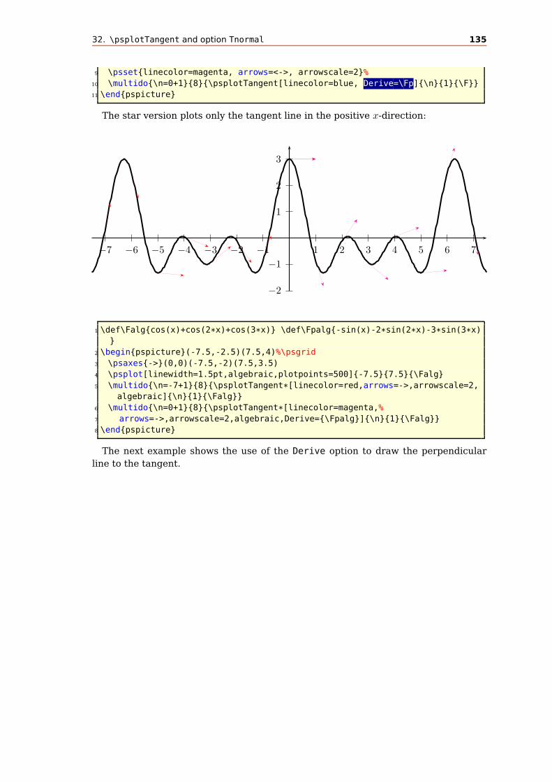
32. \psplotTangent and option Tnormal 135
9 \psset{linecolor=magenta, arrows=<->, arrowscale=2}%
10 \multido{\n=0+1}{8}{\psplotTangent[linecolor=blue, Derive=\Fp]{\n}{1}{\F}}
11 \end{pspicture}
The star version plots only the tangent line in the positive x-direction:
1
2
3
−1
−2
1 2 3 4 5 6 7−1−2−3−4−5−6−7
1 \def\Falg{cos(x)+cos(2*x)+cos(3*x)} \def\Fpalg{-sin(x)-2*sin(2*x)-3*sin(3*x)
}
2 \begin{pspicture}(-7.5,-2.5)(7.5,4)%\psgrid
3 \psaxes{->}(0,0)(-7.5,-2)(7.5,3.5)
4 \psplot[linewidth=1.5pt,algebraic,plotpoints=500]{-7.5}{7.5}{\Falg}
5 \multido{\n=-7+1}{8}{\psplotTangent*[linecolor=red,arrows=->,arrowscale=2,
algebraic]{\n}{1}{\Falg}}
6 \multido{\n=0+1}{8}{\psplotTangent*[linecolor=magenta,%
7 arrows=->,arrowscale=2,algebraic,Derive={\Fpalg}]{\n}{1}{\Falg}}
8 \end{pspicture}
The next example shows the use of the Derive option to draw the perpendicular
line to the tangent.

32.1. A polarplot example 136
0
1
2
3
4
5
6
0 1 2 3 4 5 6
1\begin{pspicture}(-0.5,-0.5)(7.25,7.25)
2 \def\Func{10 x div}
3 \psaxes[arrowscale=1.5]{->}(7,7)
4 \psplot[linewidth=2pt,algebraic
]{1.5}{5}{10/x}
5 \psplotTangent[linewidth=.5\pslinewidth,
linecolor=red,algebraic]{3}{2}{10/x}
6 \psplotTangent[linewidth=.5\pslinewidth,
linecolor=blue,algebraic,Derive=(x*x)
/10]{3}{2}{10/x}
7 \psline[linestyle=dashed](!0 /x 3 def \
Func)(!3 /x 3 def \Func)(3,0)
8\end{pspicture}
By setting the optional argument Tnormal one can plot the normal of the tangent
line. It always starts at the given point.
0
1
2
3
4
5
6
0 1 2 3 4 5 6
1\begin{pspicture}(-0.5,-0.5)(7.25,7.25)
2 \def\Func{10 x div}
3 \psaxes[arrowscale=1.5]{->}(7,7)
4 \psplot[linewidth=2pt]{1.5}{5}{\Func}
5 \psplotTangent[linewidth=1.5\pslinewidth,
linecolor=red]{3}{2}{\Func}
6 \psplotTangent[linewidth=1.5\pslinewidth,
linecolor=blue,Tnormal]{3}{2}{\Func}
7 \psline[linestyle=dashed](!0 /x 3 def \
Func)(!3 /x 3 def \Func)(3,0)
8\end{pspicture}
32.1. A polarplot example
Let’s work with the classical cardioid: r = 2(1+cos(θ)) anddr
dθ= −2 sin(θ). The Derive
option always expects the drdθ
value and uses internally the equation for the derivative
of implicitly defined functions:
dy
dx=
r′ · sin θ + x
r′ · cos θ − y
where x = r · cos θ and y = r · sin θ

32.2. A \parametricplot example 137
1
2
−1
−2
−3
1 2 3 4−1
1\begin{pspicture}(-1,-3)(5,3)%\psgrid[subgridcolor=
lightgray]
2 \psaxes{->}(0,0)(-1,-3)(5,3)
3 \psplot[polarplot,linewidth=3\pslinewidth,linecolor=
blue,%
4 plotpoints=500]{0}{360}{1 x cos add 2 mul}
5\end{pspicture}
1
2
−1
−2
−3
1 2 3 4−1
1\begin{pspicture}(-1,-3)(5,3)%\psgrid[subgridcolor=
lightgray]
2 \psaxes{->}(0,0)(-1,-3)(5,3)
3 \psplot[polarplot,linewidth=3\pslinewidth,linecolor=
blue,plotpoints=500]{0}{360}{1 x cos add 2 mul}
4 \multido{\n=0+36}{10}{%
5 \psplotTangent[polarplot,linecolor=red,arrows
=<->]{\n}{1.5}{1 x cos add 2 mul} }
6\end{pspicture}
1
2
−1
−2
−3
1 2 3 4−1
1\begin{pspicture}(-1,-3)(5,3)%\psgrid[subgridcolor=
lightgray]
2 \psaxes{->}(0,0)(-1,-3)(5,3)
3 \psplot[polarplot,linewidth=3\pslinewidth,linecolor=
blue,algebraic,plotpoints=500]{0}{6.289}{2*(1+cos(
x))}
4 \multido{\r=0.000+0.314}{21}{%
5 \psplotTangent[polarplot,Derive=-2*sin(x),
algebraic,linecolor=red,arrows=<->]{\r
}{1.5}{2*(1+cos(x))} }
6\end{pspicture}
32.2. A \parametricplot example
Let’s work with a Lissajou curve:
{x = 3.5 cos(2t)y = 3.5 sin(6t)
whose derivative is :
{x = −7 sin(2t)y = 21 cos(6t)
The parameter must be the letter t instead of x and when using the algebraic
option you must separate the two equations by a | (see example).

32.2. A \parametricplot example 138
1\def\Lissa{t dup 2 RadtoDeg mul cos 3.5 mul exch 6 mul RadtoDeg sin 3.5 mul}%
2\psset{yunit=0.6}
3\begin{pspicture}(-4,-4)(4,6)
4 \parametricplot[plotpoints=500,linewidth=3\pslinewidth]{0}{3.141592}{\Lissa}
5 \multido{\r=0.000+0.314}{11}{%
6 \psplotTangent[linecolor=red,arrows=<->]{\r}{1.5}{\Lissa} }
7 \multido{\r=0.157+0.314}{11}{%
8 \psplotTangent[linecolor=blue,arrows=<->]{\r}{1.5}{\Lissa} }
9\end{pspicture}\hfill%
10\def\LissaAlg{3.5*cos(2*t)|3.5*sin(6*t)} \def\LissaAlgDer{-7*sin(2*t)|21*cos(6*t)}%
11\begin{pspicture}(-4,-4)(4,6)
12 \parametricplot[algebraic,plotpoints=500,linewidth=3\pslinewidth]{0}{3.141592}{\
LissaAlg}
13 \multido{\r=0.000+0.314}{11}{%
14 \psplotTangent[algebraic,linecolor=red,arrows=<->]{\r}{1.5}{\LissaAlg} }
15 \multido{\r=0.157+0.314}{11}{%
16 \psplotTangent[algebraic,linecolor=blue,arrows=<->,%
17 Derive=\LissaAlgDer]{\r}{1.5}{\LissaAlg} }
18\end{pspicture}

33. Successive derivatives of a function 139
33. Successive derivatives of a function
The new PostScript function Derive has been added for plotting successive deriva-
tives of a function. It must be used with the algebraic option. This function has two
arguments:
1. a positive integer which defines the order of the derivative; obviously 0 means
the function itself!
2. a function of variable x which can be any function using common operators,
Do not think that the derivative is approximated, the internal PostScript engine will
compute the real derivative using a formal derivative engine.
The following diagram contains the plot of the polynomial:
f(x) =
14∑
i=0
(−1)ix2i
i!= 1 − x2
2+
x4
4!− x6
6!+
x8
8!− x10
10!+
x12
12!− x14
14!
and of its first 15 derivatives. It is the sequence definition of the cosine.
0 1 2 3 4 5 6 7-1
0
1
1\psset{unit=2}
2\def\getColor#1{\ifcase#1 Tan\or RedOrange\or magenta\or yellow\or green\or Orange\or
blue\or
3 DarkOrchid\or BrickRed\or Rhodamine\or OliveGreen\or Goldenrod\or Mahogany\or
4 OrangeRed\or CarnationPink\or RoyalPurple\or Lavender\fi}
5\begin{pspicture}[showgrid=true](0,-1.2)(7,1.5)
6 \psclip{\psframe[linestyle=none](0,-1.1)(7,1.1)}
7 \multido{\in=0+1}{16}{%
8 \psplot[linewidth=1pt,algebraic,linecolor=\getColor{\in}]{0}{7}
9 {Derive(\in,1-x^2/2+x^4/24-x^6/720+x^8/40320-x^10/3628800+x^12/479001600-x
^14/87178291200)}}
10 \endpsclip
11\end{pspicture}

33. Successive derivatives of a function 140
0 1 2 3-2
-1
0
1
2
3
1\begin{pspicture}[shift=-2.5,showgrid=true,linewidth=1
pt](0,-2)(3,3)
2 \psplot[algebraic]{.001}{3}{x*ln(x)} % f(x)
3 \psplot[algebraic,linecolor=red]{.05}{3}{Derive(1,x*ln
(x))} % f’(x)=1+ln(x)
4\end{pspicture}

34. Variable step for plotting a curve 141
34. Variable step for plotting a curve
34.1. Theory
As you know with the \psplot macro, the curve is plotted using a piece-wise linear
curve. The step is given by the parameter plotpoints. For each step between xi
and xi+1, the area defined between the curve and its approximation (a segment) is
majored by this formula :
|ε| ≤ M2(f)(xi+1 − xi)3
12
M2(f) is a majorant of the second deriva-
tive of f in the interval [xi;xi+1].
0 1 2 3 4 5 6-1
0
1
2
3
xn xn+1
ε
The parameter VarStep (false by default) activates the variable step algorithm. It
is set to a tolerance defined by the parameter VarStepEpsilon (default by default,
accept real value). If this parameter is not set by the user, then it is automatically
computed using the default first step given by the parameter plotpoints. Then, for
each step, f ′′(xn) and f ′′(xn+1) are computed and the smaller is used as M2(f), andthen the step is approximated. This means that the step is constant for second order
polynomials.
34.2. The cosine
Different value for the tolerance from 0.01 to 0.000 1, a factor 10 between each of them.
In black, there is the classic \psplot behavior, and in magenta the default variable
step behavior.
0 1 2 3-1
0
1
2
b
b
b
b
b
b
b b
b bb
b
b
b
b
b
b
b
bb
b b
b b b b bbbbbb
b
b
b
b
b
b
bbbbbb b b b b b
b b b b b b b b b b b bbbbbbbbbb
bbbbbbbbbb b b b b b b b b b b b b
b b b b b b b b b b b b b b b b b b b b b b b b b b b b b b b b b b b b b b b b b b b b b b b b b b
1 \psset{algebraic, VarStep=true, unit=2, showpoints=true, linecolor=red}
2 \begin{pspicture}[showgrid=true](-0,-1)(3.14,2)
3 \psplot[VarStepEpsilon=.01]{0}{3.14}{cos(x)}
4 \psplot[VarStepEpsilon=.001]{0}{3.14}{cos(x)+.15}
34.2. The cosine 142
5 \psplot[VarStepEpsilon=.0001]{0}{3.14}{cos(x)+.3}
6 \psplot[linecolor=magenta]{0}{3.14}{cos(x)+.45}
7 \psplot[VarStep=false,linewidth=1pt,linecolor=black]{-0}{3.14}{cos(x)+.6}
8 \end{pspicture}

34.3. The Napierian Logarithm 143
34.3. The Napierian Logarithm
A really classic example which gives a bad beginning, the tolerance is set to 0.001.
0 1 2 3 4 5 6 7 8 9 10 11 12 13 14 15 16-5
-4
-3
-2
-1
0
1
2
3
4
b
b
b
b
bb
bb
bb
bb b b b b b b b b b b b b b b b b b b b b b b b b b b b b b b b b b b b b b b
b
b
b
b
b
b
b
b
b
b
b
b
b
b
bbbb
bb
bb
bb
bb
bb
bb
bb
bb
b b b
b
b
b
b
b
b
b
b
b
b
b
b
b
bb
bb
1 \psset{algebraic, VarStep=true, linecolor=red, showpoints=true}
2 \begin{pspicture}[showgrid=true](0,-5)(16,4)
3 \psplot[VarStep=false, linecolor=black]{.01}{16}{ln(x)+1}
4 \psplot[linecolor=magenta]{.51}{16}{ln(x-1/2)+1/2}
5 \psplot[VarStepEpsilon=.001]{1.01}{16}{ln(x-1)}
6 \psplot[VarStepEpsilon=.01]{1.51}{16}{ln(x-1.5)-100/200}
7 \end{pspicture}

34.4. Sine of the inverse of x 144
34.4. Sine of the inverse of x
Impossible to draw, but let’s try!
0-1
0
1
b
b
b
b
b
b
b
b
b
b
b
bb
b
b b
b
bb
b
b
b
b
b
b
bb
b b
b
b
b
b
b
bb
b
b
b
b
b
b
b
b
b
b
bb
b
bb
b
b
bb
b
b
b
b b
b
b
bb b
b
b
b
bb b
b
b
b
b
bb b b b
b b
0-1
0
1
b
b
b
b
b
b
b
b
b
b
b
b
b
b
b
b
b
b
b
bb
b
b b
b
b
b
b
b
b b
b
b
bb
b
b b
b
b
bb
b
b
b b
b
b
b b
b
b
b b
b
b
bbb
b
b
b b
b
b
bb
b
b
bbb
b
b
bb b
b
b
b
b b b
b
b
b
b bb
b
b
b
b b b
b
b
b
bb b bb
b
b
bbb bb
b
b
b
bbb b bb
b
b
b
bbb b bbb
b
b
bbbb b b b
bbb
b
bbbbb b
b b b bbb
b
bb
bb
bb b b b b b b b b b b b
0-1
0
1
b
bb b
b
b
b
bb b
b
b
b
bb bb
b
b
bb bb
b
b
b
bb b
b
b
b
bb bb
b
b
b
bb bb
b
b
b
bb bb
b
b
b
bb bb
b
b
b
bb b bb
b
b
b
bb bb
b
b
b
bb b b b
b
b
b
bbb bb
b
b
b
bbb b bb
b
b
b
bb b bb
b
b
b
bbb b bbb
b
b
bbb b bbb
b
b
bbb b b bbb
b
b
bbb b b bbb
b
b
bbb bb bbbb
b
b
bbb b b bbbb
b
b
bbbb b b b bbb
b
b
bbbb b b bbbbb
bbbbbb b b b b bbbb
bbbbb b b b b bbbbbb
bbbbb bb b b b b bbbbb
bbbbb b b b b b b bb bbbbbbbbbb bb bb b b b b b b b b
bbbbbbbb b b b b b b b b b b b b
b bb bbbbbbbbb bb bb bb b b b
b b b b b b b b b b b b bbbbbb b b b b b b b b b b b b b b b b b b b b b b b b b b b b b b b b
0-1
0
1
b
b
b b
b
b
b
b
b
b
b
b
b b
b
b
b b
b
b
b
b
bb b b
bb
bb
bb
bb
bb b b b b b b b b b b b b b b
1 \psset{xunit=64,algebraic,VarStep,linecolor=red,showpoints=true,linewidth=1
pt}
2 \begin{pspicture}[showgrid=true](0,-1)(.5,1)
3 \psplot[VarStepEpsilon=.0001]{.01}{.25}{sin(1/x)}
4 \end{pspicture}\\
5 \begin{pspicture}[showgrid=true](0,-1)(.5,1)
6 \psplot[VarStepEpsilon=.00001]{.01}{.25}{sin(1/x)}
7 \end{pspicture}\\
8 \begin{pspicture}[showgrid=true](0,-1)(.5,1)
9 \psplot[VarStepEpsilon=.000001]{.01}{.25}{sin(1/x)}
10 \end{pspicture}\\
11 \begin{pspicture}[showgrid=true](0,-1)(.5,1)
12 \psplot[VarStep=false, linecolor=black]{.01}{.25}{sin(1/x)}
13 \end{pspicture}
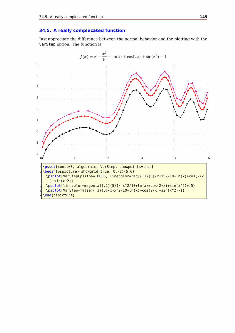
34.5. A really complecated function 145
34.5. A really complecated function
Just appreciate the difference between the normal behavior and the plotting with the
varStep option. The function is:
f(x) = x − x2
10+ ln(x) + cos(2x) + sin(x2) − 1
0 1 2 3 4 5-2
-1
0
1
2
3
4
5
6
b
b
b
b
b
bb
bb
bb
b b b b bb
bb b b b
b
b
b
b
b
b
b
b
bb b b b
b
b
b
bb b b
b
b
b
bb b b
b
b
b
b
b
bb b
bb
b
b
bb b b
b
b
b
b
bb bb
b
b b
b
b
b
b
b
b b
b
b b
b
b
b
bb
b
b
b
b
b
b
b
b
bb
b
b b
b
bb
b
b
b
b
b
b
bb
bb
bb
b b b b bb
bb
b b b
b
b
b
b
b
b
b b
b
b
b
bb
b
b
b b
b
b
bb
b
b
b
b
b
b b
b
1 \psset{xunit=3, algebraic, VarStep, showpoints=true}
2 \begin{pspicture}[showgrid=true](0,-2)(5,6)
3 \psplot[VarStepEpsilon=.0005, linecolor=red]{.1}{5}{x-x^2/10+ln(x)+cos(2*x
)+sin(x^2)}
4 \psplot[linecolor=magenta]{.1}{5}{x-x^2/10+ln(x)+cos(2*x)+sin(x^2)+.5}
5 \psplot[VarStep=false]{.1}{5}{x-x^2/10+ln(x)+cos(2*x)+sin(x^2)-1}
6 \end{pspicture}

34.6. A hyperbola 146
34.6. A hyperbola
b b b b b b b b b b b b b b b b b b b b b b b b b b b b b b b b b b b b b b b b b b b bbbb
b
b
b
b
b
b
b
b
bbbbbbbbb b b b b b b b b b b b b b b b b b
1
2
3
4
5
−1
−2
−3
−4
1 2 3 4 5 6 7 8−1−2−3−4−5
1 \psset{algebraic, showpoints=true, unit=0.75}
2 \begin{pspicture}(-5,-4)(9,6)
3 \psplot[linecolor=black]{-5}{1.8}{(x-1)/(x-2)}
4 \psplot[VarStep=true, VarStepEpsilon=.001, linecolor=red]{2.2}{9}{(x-1)/(x
-2)}
5 \psaxes{->}(0,0)(-5,-4)(9,6)
6 \end{pspicture}
34.7. Successive derivatives of a polynomial
0 1 2 3 4 5 6 7-1
0
1b
bb
b
b
b
b
b
b
bb
b b bb
b
b
b
b
b
b
bb b b
b
b
b
b
b
b b
b
b
b
b
bb b b
b
b
b
b
b
b
b
b
bb b b
bb
b
b
b
b
b
b
b
b
b
b
b
b
bb
b
b
b
b
b
b
b
bb
b b bb
b
b
b
b
b
b
b
b
b
b
b
b
b
b
b
b
b
b
b
b
b
b
b
bb b b
b
b
b
b
b
b
b
b
bb
bb b
bb
b
b
b
b
b
b
b
b
b
b
b
b
b
b
b
bb
b
b
b
b
b
b
b
bb
b b bb
b
bb
bb b b
b
b
b
b
b
b
b
b
b
b
b
b
b
b
b
b
b
b
b
b
b
b
b
b
b
b
bb b b
b
b
b
b
b
b
b
bb b b
b
b
b
b
b
b
b
b
b
b
b
b
b
b
b
b
b
b
b
b
b
b
b
b
b
b
b
b
b
b
bb
b
b
b
b
b
b
b
bb
b bb
b
b
b
b
b
b
b
b
b
b
b
b
b
b
b
b
b
b
b
b
b
b
b
b
b
b
b
b
b
b
b
b
b
b
b
b
b
b
b
b
b
b
bb b b
b
b
b
b
b
b
b
b
b
b
b
b
b
b
b
b
b
b
b
b
b
b
b
b
b
b
b
b
b
b
b
b
b
b
b
b
b
b
b
b
b
b
b
b
b
b
bb
b
b
b
b
b
b
b
b
b
b
b
b
b
b
b
b
b
b
b
b
b
b
b
b
b
b
b
b
b
b
b
b
b
b
b
b
b
b
b
b
b
b
b
b
b
b
b
b
b
b
b
b
b
b
b
b
b
bb b b
b
b
bb b b
b
b
b
b
b
b
b
b
b
b
b
b
b
b
b
b
b
b
b
b
b
b
b
b
b
b
b
b
b
b
b
b
b
b
b
b
b
b
b
b
b
b
b
bb
b
b
b
b
b
b
bb b b
b
b
b
b
b
b
b
b
b
b
b
b
b
b
b
b
b
b
b
b
b
b
b
b
b
b
b
b
b
b
b
b
b
b
b
b
b
b
b
b
b
b
b
b
b
bb
b bb
b
b
b
b
b
b
b
b
b
b
b
b
b
b
b
b
b
b
b
b
b
b
b
b
b
b
b
b
b
b
b
b
b
b
b
b
b
b
bb
b
b
b
b
b
b
b
b
b
b
b
b
b
b
b
b
b
b
b
b
b
b
b
b
b
b
b
b
b
b
b
b
b
b
b
b
b
b b b b b b b
b b b b b b b
1 \psset{unit=2, algebraic=true, VarStep=true, showpoints=true, VarStepEpsilon
=.001}
2 \def\getColor#1{\ifcase#1 Tan\or RedOrange\or magenta\or yellow\or green\or
Orange\or blue\or
3 DarkOrchid\or BrickRed\or Rhodamine\or OliveGreen\or Goldenrod\or Mahogany
\or

34.7. Successive derivatives of a polynomial 147
4 OrangeRed\or CarnationPink\or RoyalPurple\or Lavender\fi}
5 \begin{pspicture}[showgrid=true](0,-1.2)(7,1.5)
6 \psclip{\psframe[linestyle=none](0,-1.1)(7,1.1)}
7 \multido{\in=0+1}{16}{%
8 \psplot[algebraic=true, linecolor=\getColor{\in}]{0.1}{7}
9 {Derive(\in,Sum(i,0,1,7,(-1)^i*x^(2*i)/Fact(2*i)))}}
10 \endpsclip
11 \end{pspicture}

34.8. The variable step algorithm together with the IfTE primitive 148
34.8. The variable step algorithm together with the IfTE primitive
-7 -6 -5 -4 -3 -2 -1 0 1 2-2
-1
0
1
2
3
4 b
b
b
b
b
b
b
b
b
bb b b b b b b b b b b b b
bb
b
b
b
b
b
b
b
b
b
bb
b
b
b
b
b
b b b b b b b b b b b b b b b b b b b b bbb
b
b
b
b
b
b
b
b
b
b
b
b
b
b
b
b
b
b
b
b
b
b
b
b
b
b
bb b b b
bb
b
b
b
b
b
b
1 \psset{unit=1.5, algebraic, VarStep, showpoints=true, VarStepEpsilon=.001}
2 \begin{pspicture}[showgrid=true](-7,-2)(2,4)
3 \psplot{-7}{2}{IfTE(x<-5,-(x+5)^3/2,IfTE(x<0,0,x^2))}
4 \psplot{-7}{2}{5*x/9+26/9}
5 \psplot[linecolor=blue]{-7}{2}{(x+7)^30/9^30*4.5-1/2}
6 \psplot[linecolor=red]{-6.9}{2}
7 {IfTE(x<-6,ln(x+7),IfTE(x<-3,x+6,IfTE(x<0.1415926,sin(x+3)+3,3.1415926-
x)))}
8 \end{pspicture}

34.9. Using \parametricplot 149
34.9. Using \parametricplot
\parametricplot [Options] {t0}{t1} [PS commands] {x(t) y(t)}
-1 0 1-1
0
1
b
b
b
b
b
b
bb
bb
bb b b b b b b
bbbb
bb
b
b
b
b
b
b
b
b
bb
bbbbb b b b b b b b
bb
bb
b
b
b
b
b
b
b
b
b
b
b
bb
bb
bb
bbbbbbbbbbbbb
b
b
b
b
b
b
b
b
bbbbbbbbbbbbbb
bb
bb
b
b
b
b
b
bb
-1 0 1-1
0
1
1 \psset{unit=3}
2 \begin{pspicture}[showgrid=true](-1,-1)(1,1)
3 \parametricplot[algebraic=true,linecolor=red,VarStep=true, showpoints=true,
4 VarStepEpsilon=.0001]
5 {-3.14}{3.14}{cos(3*t)|sin(2*t)}
6 \end{pspicture}
7 \begin{pspicture}[showgrid=true](-1,-1)(1,1)
8 \parametricplot[algebraic=true,linecolor=blue,VarStep=true, showpoints=false
,
9 VarStepEpsilon=.0001]
10 {-3.14}{3.14}{cos(3*t)|sin(2*t)}
11 \end{pspicture}
-1 0 1-1
0
1
b
b
b
b
b
b
b
b
bb
bbbbbbbbbb
bb
b
b
b
b
b
b
b
b
bbbb
bb
bbbbbb
bb
bbbbb
b
b
b
b
b
b
b
b
bb
bbbbb
bbbbbb
b
b
b
b
b
b
b
b
b
b
b
b
b
b
b
bb
bb b b b b b
bb
bb
bb
b
b
b
b
b
b
b
b
bbbbb
bb
b b b b bb
bbbbbb
b
b
b
b
b
b
b
b
bb
bb
bb b b b b b b
bb
b
b
b
b
b
b
b
b
b
b
b
b
b
b
bb
bbbbbbb b
bbb
b
b
b
b
b
b
b
b
b
b
bbb
bb
bbbbbbb
bb
bbbbb
b
b
b
b
b
b
b
b
bb
bbbbb
bbbbbb
b
b
b
b
b
b
b
b
b
b
b
b
b
b
b
bb
bb b b b b b
bb
bb
b
b
b
b
b
b
b
b
b
b
bbbbb
bb b b b b b
bbbbbbb
b
b
b
b
b
b
b
b
bb
bbbb b b b b b b
bb
b
b
b
b
b
b
b
b
b
b
b
b
b
b
bb
bbbbbbb b
bbb
b
b
b
b
b
b
b
b
b
b
bbb
bb
bbbbbbb
bb
bbbbb
b
b
b
b
b
b
b
b
bb
bbbbb
bbbbbb
b
b
b
b
b
b
b
b
b
b
b
b
b
b
b
bb
bb b b b b b
bb
bb
b
b
b
b
b
b
b
b
b
b
bbbbb
bb b b b b b
bbbbbbb
b
b
b
b
b
b
b
b
bb
bbbb b b b b b b
bb
b
b
b
b
b
b
b
b
b
b
b
b
b
b
bb
bbbbbbb b
bbb
b
b
b
b
b
b
b
b
b
b
bbb
bb
bbbbbbb
bb
bbbbb
b
b
b
b
b
b
b
b
bb
bbbbb
bbbbbb
b
b
b
b
b
b
b
b
b
b
b
b
b
b
b
bb
bb b b b b b
bb
bb
b
b
b
b
b
b
b
b
b
b
bbbbb
bb b b b b b
bbbbbbb
b
b
b
b
b
b
b
b
bb
bbbb b b b b b b
bb
b
b
b
b
b
b
b
b
b
b
b
b
b
b
bb
bbbbbbb b
bbb
b
b
b
b
b
b
b
b
b
b
bbb
bb
bbbbbbb
bb
bbbbb
b
b
b
b
b
b
b
b
bb
bbbbb
bbbbbb
b
b
b
b
b
b
b
b
b
b
b
b
b
b
b
bb
bb b b b b b
bb
bb
b
b
b
b
b
b
b
b
b
b
bbbbb
bb b b b b b
bbbbbbb
b
b
b
b
b
b
b
b
bb
bbbb b b b b b b
bb
b
b
b
b
b
b
b
b
b
b
b
b
b
b
bb
bbbbbbb b
bbb
b
b
b
b
b
b
b
b
b
b
bbb
bb
bbbbbbb
bb
bbbbb
b
b
b
b
b
b
b
b
bb
bbbbb
bbbbbb
b
b
b
b
b
b
b
b
b
b
b
b
b
b
b
bb
bb b b b b b
bb
bb
b
b
b
b
b
b
b
b
b
b
bbbbb
bb b b b b b
bbbbbbb
b
b
b
b
b
b
b
b
bb
bbbb b b b b b b
bb
b
b
b
b
b
b
b
b
b
b
b
b
b
b
bb
bbbbbbb b
bbb
b
b
b
b
b
b
b
b
b
b
bbb
bb
bbbbbbb
bb
bbbbb
b
b
b
b
b
b
b
b
bb
bbbbb
bbbbbb
b
b
b
b
b
b
b
b
b
b
b
b
b
b
b
bb
bb b b b b b
bb
bb
b
b
b
b
b
b
b
b
b
b
bbbbb
bb b b b b b
bbbbbbb
b
b
b
b
b
b
b
b
bb
bbbb b b b b b b
bb
b
b
b
b
b
b
b
b
b
b
b
b
b
b
bb
bbbbbbb b
bbb
b
b
b
b
b
b
b
b
b
b
bbb
bb
bbbbbbb
bb
bbbbb
b
b
b
b
b
b
b
b
bb
bbbbb
bbbbbb
b
b
b
b
b
b
b
bb
-1 0 1-1
0
1
1 \psset{unit=2.5}
2 \begin{pspicture}[showgrid=true](-1,-1)(1,1)
3 \parametricplot[algebraic=true,linecolor=red,VarStep=true, showpoints=true,
4 VarStepEpsilon=.0001]
5 {0}{47.115}{cos(5*t)|sin(3*t)}
6 \end{pspicture}
7 \begin{pspicture}[showgrid=true](-1,-1)(1,1)

35. New math functions and their derivatives 150
8 \parametricplot[algebraic=true,linecolor=blue,VarStep=true, showpoints=false
,
9 VarStepEpsilon=.0001]
10 {0}{47.115}{cos(5*t)|sin(3*t)}
11 \end{pspicture}
0 1 2 3 4 5 6 7 8 9 10 11 12 130
1
2
bb
b
b
b
bb b
b
b
b
b
b bb
b
b
b
bb b
b
b
b
bb b
0 1 2 3 4 5 6 7 8 9 10 11 12 130
1
2
1 \psset{xunit=.5}
2 \begin{pspicture}[showgrid=true](0,0)(12.566,2)
3 \parametricplot[algebraic,linecolor=red,VarStep, showpoints=true,
4 VarStepEpsilon=.01]{0}{12.566}{t+cos(-t-Pi/2)|1+sin(-t-Pi/2)}
5 \end{pspicture}
6 %
7 \begin{pspicture}[showgrid=true](0,0)(12.566,2)
8 \parametricplot[algebraic,linecolor=blue,VarStep, showpoints=false,
9 VarStepEpsilon=.001]{0}{12.566}{t+cos(-t-Pi/2)|1+sin(-t-Pi/2)}
10 \end{pspicture}
35. New math functions and their derivatives
35.1. The inverse sine and its derivative
-1 0 1-2
-1
0
1
2
-1 0 1-2
-1
0
1
2
bbb
b
b
b
b
b
b
b
b
b
bb b bb b bb bb bb b
-1 0 10
1
2
3
4 b
b
b
b
b
b
b
bbb b b b
bbbb
b
b
b
b
b
b
b
-1 0 10
1
2
3
4 b
b
b
b
b
b
b
b
bbbbbbbb b b b b b b b b b b
b bb bbbbbbbb
b
b
b
b
b
b
b
bb
1 \psset{unit=1.5}
2 \begin{pspicture}[showgrid=true](-1,-2)(1,2)
3 \psplot[linecolor=blue,algebraic]{-1}{1}{asin(x)}
4 \end{pspicture}
5 \hspace{1em}
6 \psset{algebraic, VarStep, VarStepEpsilon=.001, showpoints=true}
7 \begin{pspicture}[showgrid=true](-1,-2)(1,2)

35.2. The inverse cosine and its derivative 151
8 \psplot[linecolor=blue]{-.999}{.999}{asin(x)}
9 \end{pspicture}
10 \hspace{1em}
11 \begin{pspicture}[showgrid=true](-1,0)(1,4)
12 \psplot[linecolor=red]{-.97}{.97}{Derive(1,asin(x))}
13 \end{pspicture}
14 \hspace{1em}
15 \psset{algebraic, VarStep, VarStepEpsilon=.0001, showpoints=true}
16 \begin{pspicture}[showgrid=true](-1,0)(1,4)
17 \psplot[linecolor=red]{-.97}{.97}{Derive(1,asin(x))}
18 \end{pspicture}
35.2. The inverse cosine and its derivative
-1 0 10
1
2
3
-1 0 10
1
2
3 bbb
b
b
b
b
b
b
b
b
b
bb b b b b b b b b bb b
-1 0 1-4
-3
-2
-1
b
b
b
b
b
b
b
bbb b b b
bbbb
b
b
b
b
b
b
b -1 0 1-4
-3
-2
-1
b
b
b
b
b
b
b
b
bbbbbbbb bb bb b b b b b b b b b b
bbbbbbb
b
b
b
b
b
b
b
bb
1 \psset{unit=1.5}
2 \begin{pspicture}[showgrid=true](-1,0)(1,3)
3 \psplot[linecolor=blue,algebraic]{-1}{1}{acos(x)}
4 \end{pspicture}
5 \hspace{1em}
6 \psset{algebraic, VarStep, VarStepEpsilon=.001, showpoints=true}
7 \begin{pspicture}[showgrid=true](-1,0)(1,3)
8 \psplot[linecolor=blue]{-.999}{.999}{acos(x)}
9 \end{pspicture}
10 \hspace{1em}
11 \begin{pspicture}[showgrid=true](-1,-4)(1,-1)
12 \psplot[linecolor=red]{-.97}{.97}{Derive(1,acos(x))}
13 \end{pspicture}
14 \hspace{1em}
15 \psset{algebraic, VarStep, VarStepEpsilon=.0001, showpoints=true}
16 \begin{pspicture}[showgrid=true](-1,-4)(1,-1)
17 \psplot[linecolor=red]{-.97}{.97}{Derive(1,acos(x))}
18 \end{pspicture}

35.3. The inverse tangent and its derivative 152
35.3. The inverse tangent and its derivative
-4 -3 -2 -1 0 1 2 3 4-2
-1
0
1
2
b b b b b b b b b bb b b
b bb b
b bb bb b b b b b b b b b b b b b b b b b b b b b b b b b b
-4 -3 -2 -1 0 1 2 3 4-2
-1
0
1
2
b b b b b bb
bb
b
b
b
bb
bb
b b b b b b b
b b b b b b bb
bbb b b b
bb
bb b b b b b b
1 \begin{pspicture}[showgrid=true](-4,-2)(4,2)
2 \psset{algebraic=true}
3 \psplot[linecolor=blue,linewidth=1pt]{-4}{4}{atg(x)}
4 \psplot[linecolor=red,VarStep, VarStepEpsilon=.0001, showpoints=true
]{-4}{4}{Derive(1,atg(x))}
5 \end{pspicture}
6 \hspace{1em}
7 \begin{pspicture}[showgrid=true](-4,-2)(4,2)
8 \psset{algebraic, VarStep, VarStepEpsilon=.001, showpoints=true}
9 \psplot[linecolor=blue]{-4}{4}{atg(x)}
10 \psplot[linecolor=red]{-4}{4}{Derive(1,atg(x))}
11 \end{pspicture}

35.4. Hyperbolic functions 153
35.4. Hyperbolic functions
1
2
3
−1
−2
−3
−4
1 2−1−2−3
b
b
b
b
b
b
b
b
b
b
b
b
b
b
b
b
b
b
b
bb
b
b
b
b
b
bbbbb b b b b
bbb
b
b
b
b
bb
b b b b b b bbbb
bbbb b b b b b b1
2
3
−1
−2
−3
−4
1 2−1−2−3
1 \begin{pspicture}(-3,-4)(3,4)
2 \psset{algebraic=true}
3 \psplot[linecolor=red,linewidth=1pt]{-2}{2}{sh(x)}
4 \psplot[linecolor=blue,linewidth=1pt]{-2}{2}{ch(x)}
5 \psplot[linecolor=green,linewidth=1pt]{-3}{3}{th(x)}
6 \psaxes{->}(0,0)(-3,-4)(3,4)
7 \end{pspicture}
8 \hspace{1em}
9 \begin{pspicture}(-3,-4)(3,4)
10 \psset{algebraic=true, VarStep=true, VarStepEpsilon=.001, showpoints=true}
11 \psplot[linecolor=red,linewidth=1pt]{-2}{2}{sh(x)}
12 \psplot[linecolor=blue,linewidth=1pt]{-2}{2}{ch(x)}
13 \psplot[linecolor=green,linewidth=1pt]{-3}{3}{th(x)}
14 \psaxes{->}(0,0)(-3,-4)(3,4)
15 \end{pspicture}

35.4. Hyperbolic functions 154
1
2
3
−1
−2
−3
−4
1 2−1−2−3
b
b
b
b
b
bbbbb b b b b
bbb
b
b
b
b
bb
b
b
b
b
b
b
b
b
b
b
b
b
b
b
b
b
b
b
b
bb
b b b b b bbbbb b
b b bbbbb b b b b b
1
2
3
−1
−2
−3
−4
1 2−1−2−3
1 \begin{pspicture}(-3,-4)(3,4)
2 \psset{algebraic=true,linewidth=1pt}
3 \psplot[linecolor=red,linewidth=1pt]{-2}{2}{Derive(1,sh(x))}
4 \psplot[linecolor=blue,linewidth=1pt]{-2}{2}{Derive(1,ch(x))}
5 \psplot[linecolor=green,linewidth=1pt]{-3}{3}{Derive(1,th(x))}
6 \psaxes{->}(0,0)(-3,-4)(3,4)
7 \end{pspicture}
8 \hspace{1em}
9 \begin{pspicture}(-3,-4)(3,4)
10 \psset{algebraic=true, VarStep=true, VarStepEpsilon=.001, showpoints=true}
11 \psplot[linecolor=red,linewidth=1pt]{-2}{2}{Derive(1,sh(x))}
12 \psplot[linecolor=blue,linewidth=1pt]{-2}{2}{Derive(1,ch(x))}
13 \psplot[linecolor=green,linewidth=1pt]{-3}{3}{Derive(1,th(x))}
14 \psaxes{->}(0,0)(-3,-4)(3,4)
15 \end{pspicture}
1
2
−1
−2
−3
1 2 3 4 5 6−1−2−3−4−5−6−7

35.4. Hyperbolic functions 155
bb
bb
bb
bb
bb
bb
bb
b
b
b
bb
bb
bb
bb
bb
bb
b b
bbbbbbbb
bb
bb
bb
bb
bb b
b
b
b
b
bbbbbb
bbbbbbbbbbb
b b
1
2
−1
−2
−3
1 2 3 4 5 6−1−2−3−4−5−6−7
1 \begin{pspicture}(-7,-3)(7,3)
2 \psset{algebraic=true}
3 \psplot[linecolor=red,linewidth=1pt]{-7}{7}{Argsh(x)}
4 \psplot[linecolor=blue,linewidth=1pt]{1}{7}{Argch(x)}
5 \psplot[linecolor=green,linewidth=1pt]{-.99}{.99}{Argth(x)}
6 \psaxes{->}(0,0)(-7,-3)(7,3)
7 \end{pspicture}\\[\baselineskip]
8 \begin{pspicture}(-7,-3)(7,3)
9 \psset{algebraic, VarStep, VarStepEpsilon=.001, showpoints=true}
10 \psplot[linecolor=red,linewidth=1pt]{-7}{7}{Argsh(x)}
11 \psplot[linecolor=blue,linewidth=1pt]{1.001}{7}{Argch(x)}
12 \psplot[linecolor=green,linewidth=1pt]{-.99}{.99}{Argth(x)}
13 \psaxes{->}(0,0)(-7,-3)(7,3)
14 \end{pspicture}
1
2
3
4
5
0 1 2 3 4 5 6−1−2−3−4−5−6−7

35.4. Hyperbolic functions 156
b b b b b b b b bb
b b b b b b bb
b b b b b b b b b b
b
b
b
b
b
b
b
bbbbbb b b b b b b b b b
b
b
b
b
b
b
bbbb b b b b
bbbb
b
b
b
b
b
bb
1
2
3
4
5
0 1 2 3 4 5 6−1−2−3−4−5−6−7
1 \begin{pspicture}(-7,-0.5)(7,6)
2 \psset{algebraic=true}
3 \psplot[linecolor=red,linewidth=1pt]{-7}{7}{Derive(1,Argsh(x))}
4 \psplot[linecolor=blue,linewidth=1pt]{1.014}{7}{Derive(1,Argch(x))}
5 \psplot[linecolor=green,linewidth=1pt]{-.9}{.9}{Derive(1,Argth(x))}
6 \psaxes{->}(0,0)(-7,0)(7,6)
7 \end{pspicture}\\[\baselineskip]
8 \begin{pspicture}(-7,-0.5)(7,6)
9 \psset{algebraic=true}
10 \psset{algebraic=true, VarStep=true, VarStepEpsilon=.001, showpoints=true}
11 \psplot[linecolor=red,linewidth=1pt]{-7}{7}{Derive(1,Argsh(x))}
12 \psplot[linecolor=blue,linewidth=1pt]{1.014}{7}{Derive(1,Argch(x))}
13 \psplot[linecolor=green,linewidth=1pt]{-.9}{.9}{Derive(1,Argth(x))}
14 \psaxes{->}(0,0)(-7,0)(7,6)
15 \end{pspicture}

36. \psplotDiffEqn – solving diffential equations 157
36. \psplotDiffEqn – solving diffential equations
A differential equation of first order is like
y′ = f(x, y, y′) (1)
where y is a function of x. We define some vectors Y = [y, y′, · · · , y(n−1)] and Y ′ =[y′, y′′, · · · , yn], depending on the order n. The syntax of the macro is
\psplotDiffEqn [Options] {x0}{x1}{y0}{f(x,y,y’,...)}
• options: the \psplotDiffEqn specific options and all other of PSTricks, which
make sense;
• x0: the start value;
• x1: the end value of the definition interval;
• y0: the initial values for y(x0) y′(x0) . . .;• f(x, y, y′, ...): the differential equation, depending to the number of initial values,
e.g.: {0 1} for y0 are two initial values, so that we have a differential equation
of second order f(x, y, y′) and the macro leaves y y′ on the stack.
The new options are:
• method: integration method (euler for order 1 euler method, rk4 for 4th order
Runge-Kutta method);
• whichabs: select the abscissa for plotting the graph, by default it is x, but youcan specify a number which represent a position in the vector y;
• whichord: same as precedent for the ordinate, by default y(0);• plotfuncx: describe a ps function for the abscissa, parameter whichabs be-
comes useless;
• plotfuncy: idem for the ordinate;
• buildvector: boolean parameter for specifying the input-output of the f de-
scription:
true (default): y is put on the stack element by element, y′ must be given in the
same way;
false : y is put on the stack as a vector, y′ must be returned in the same way;
• algebraic: algebraic description for f , buildvector parameter is useless when
activating this option.

36.1. Variable step for differential equations 158
36.1. Variable step for differential equations
A new algorithm has been added for adjusting the step according to the variations of
the curve. The parameter method has a new possible value : varrkiv to activate the
Runge-Kutta method with variable step, then the parameter varsteptol (real value;
.01 by default) can control the tolerance of the algortihm.
0 1 2 3 4 5 6 7 8 9 100
1 b
b
b
bb b b b b
b
b
b
b
b
bb b b b b b b b b b b
b
b
b
b
b
b
bb
b b b b b b b b b b b b b b b
b
b
b
b
b
b
b
b
bb
bb
b b b b b b b b b b b b b b b b b b b b b b b b b b b b
RK ordre 4 : ε < 10−1
RK ordre 4 : ε < 10−2
RK ordre 4 : ε < 10−3
RK ordre 4 : ε < 10−4
solution exacte
Figure 1: Equation y′ = −y with y0 = 1.
1 \def\Funct{neg}\def\FunctAlg{-y[0]}
2 \psset{xunit=1.5, yunit=8, showpoints=true}
3 \begin{pspicture}[showgrid=true](0,0)(10,1.2)
4 \psplot[linewidth=6\pslinewidth, linecolor=green, showpoints=false
]{0}{10}{Euler x neg exp}
5 \psplotDiffEqn[linecolor=magenta, method=varrkiv, varsteptol=.1,
plotpoints=2]{0}{10}{1}{\Funct}
6 \rput(0,.0){\psplotDiffEqn[linecolor=blue, method=varrkiv, varsteptol=.01,
plotpoints=2]{0}{10}{1}{\Funct}}
7 \rput(0,.1){\psplotDiffEqn[linecolor=Orange, method=varrkiv, varsteptol
=.001, plotpoints=2]{0}{10}{1}{\Funct}}
8 \rput(0,.2){\psplotDiffEqn[linecolor=red, method=varrkiv, varsteptol
=.0001, plotpoints=2]{0}{10}{1}{\Funct}}
9 \psset{linewidth=4\pslinewidth,showpoints=false}
10 \rput*(3.3,.9){\psline[linecolor=magenta](-.75cm,0)}
11 \rput*[l](3.3,.9){\small RK ordre 4 : $\varepsilon<10^{-1}$}
12 \rput*(3.3,.8){\psline[linecolor=blue](-.75cm,0)}
13 \rput*[l](3.3,.8){\small RK ordre 4 : $\varepsilon<10^{-2}$}
14 \rput*(3.3,.7){\psline[linecolor=Orange](-.75cm,0)}

36.1. Variable step for differential equations 159
15 \rput*[l](3.3,.7){\small RK ordre 4 : $\varepsilon<10^{-3}$}
16 \rput*(3.3,.6){\psline[linecolor=red](-.75cm,0)}
17 \rput*[l](3.3,.6){\small RK ordre 4 : $\varepsilon<10^{-4}$}
18 \rput*(3.3,.5){\psline[linecolor=green](-.75cm,0)}
19 \rput*[l](3.3,.5){\small solution exacte}
20 \end{pspicture}
0
1
−1
1 2 3 4 5 6 7 8 9
b bbb
b
b
b
b
b
b
b
b
b
bb b b
bb
b
b
b
b
b
b
b
b
b
bbb b b
bb
b
b
b
b
b
b
b
b
bbb b b
bbb
b
b
b
b
b
b
b
b bb
b
b
b
b
b b
b
b
b
b
b b
b
b
b
b
bb
b
b b
b
b
b
b
bb
b
b
b
b
bb
b
b
b
b
bb
b
bb
b
b
b
b
b
b
b
b
b
bb
b
b
b
b
b
b
b
b
b
b
bb
b
b
b
b
b
b
b
b
b
b
bb
b
b
bbb
b
b
b
b
b
b
b
b
b
b
b
b
bb b
b
b
b
b
b
b
b
b
b
b
b
b
bb
b b
b
b
b
b
b
b
b
b
b
b
b
b
b
b
b bb
b
b
ε < 10−1
ε < 10−2
ε < 10−3
ε < 10−4
ε < 10−5
solution exacte
Figure 2: Equation y′′ = −y
1 \def\Funct{exch neg}
2 \psset{xunit=1.5, yunit=5, method=varrkiv, showpoints=true}%%
3 \def\quatrepi{12.5663706144}
4 \begin{pspicture}(0,-1)(10,1.3)
5 \psaxes{->}(0,0)(0,-1)(10,1.3)
6 \psplot[linewidth=4\pslinewidth, linecolor=green, algebraic=true]{0}{10}{
cos(x)}
7 \rput(0,.0){\psplotDiffEqn[linecolor=magenta, plotpoints=7, varsteptol
=.1]{0}{10}{1 0}{\Funct}}
8 \rput(0,.0){\psplotDiffEqn[linecolor=blue, plotpoints=201, varsteptol
=.01]{0}{10}{1 0}{\Funct}}
9 \rput(0,.1){\psplotDiffEqn[linewidth=2\pslinewidth, linecolor=red,
varsteptol=.001]{0}{10}{1 0}{\Funct}}

36.1. Variable step for differential equations 160
10 \rput(0,.2){\psplotDiffEqn[linecolor=black, varsteptol=.0001]{0}{10}{1
0}{\Funct}}
11 \rput(0,.3){\psplotDiffEqn[linecolor=Orange, varsteptol=.00001]{0}{10}{1
0}{\Funct}}
12 \psset{linewidth=4\pslinewidth,showpoints=false}
13 \rput*(2.3,.9){\psline[linecolor=magenta](-.75cm,0)}
14 \rput*[l](2.3,.9){\small $\varepsilon<10^{-1}$}
15 \rput*(2.3,.8){\psline[linecolor=blue](-.75cm,0)}
16 \rput*[l](2.3,.8){\small $\varepsilon<10^{-2}$}
17 \rput*(2.3,.7){\psline[linecolor=red](-.75cm,0)}
18 \rput*[l](2.3,.7){\small $\varepsilon<10^{-3}$}
19 \rput*(2.3,.6){\psline[linecolor=black](-.75cm,0)}
20 \rput*[l](2.3,.6){\small $\varepsilon<10^{-4}$}
21 \rput*(2.3,.5){\psline[linecolor=Orange](-.75cm,0)}
22 \rput*[l](2.3,.5){\small $\varepsilon<10^{-5}$}
23 \rput*(2.3,.4){\psline[linecolor=green](-.75cm,0)}
24 \rput*[l](2.3,.4){\small solution exacte}
25 \end{pspicture}
0
1
2
3
4
5
6
7
8
9
10
0 1 2
b b b b b b b b b b bb b b b b
b b bb b b
b bb bb bb bb bbbbbbbbbbbbbbbbb
b
bb
b b b
b
b
b
b
bb
b b b
b
b
b
b
bb
b b b
b
b
b
b
bb
b b bb
b
b
b
b
b
b
b
b
b
b b b bb
b
b
b
b
b
b
b
b
b
ε < 10−1
ε < 10−2
ε < 10−3
ε < 10−4
ε < 10−5solution exacte
Figure 3: Equation y′′ = y
1 \def\Funct{exch}
2 \psset{xunit=4, yunit=1, method=varrkiv, showpoints=true}%%

36.1. Variable step for differential equations 161
3 \def\quatrepi{12.5663706144}
4 \begin{pspicture}(0,-0.5)(3,11)
5 \psaxes{->}(0,0)(3,11)
6 \psplot[linewidth=4\pslinewidth, linecolor=green, algebraic=true]{0}{3}{ch
(x)}
7 \rput(0,.0){\psplotDiffEqn[linecolor=magenta, varsteptol=.1]{0}{3}{1 0}{\
Funct}}
8 \rput(0,.3){\psplotDiffEqn[linecolor=blue, varsteptol=.01]{0}{3}{1 0}{\
Funct}}
9 \rput(0,.6){\psplotDiffEqn[linecolor=red, varsteptol=.001]{0}{3}{1 0}{\
Funct}}
10 \rput(0,.9){\psplotDiffEqn[linecolor=black, varsteptol=.0001]{0}{3}{1 0}{\
Funct}}
11 \rput(0,1.2){\psplotDiffEqn[linecolor=Orange, varsteptol=.00001]{0}{3}{1
0}{\Funct}}
12 \psset{linewidth=4\pslinewidth,showpoints=false}
13 \rput*(2.3,.9){\psline[linecolor=magenta](-.75cm,0)}
14 \rput*[l](2.3,.9){\small $\varepsilon<10^{-1}$}
15 \rput*(2.3,.8){\psline[linecolor=blue](-.75cm,0)}
16 \rput*[l](2.3,.8){\small $\varepsilon<10^{-2}$}
17 \rput*(2.3,.7){\psline[linecolor=red](-.75cm,0)}
18 \rput*[l](2.3,.7){\small $\varepsilon<10^{-3}$}
19 \rput*(2.3,.6){\psline[linecolor=black](-.75cm,0)}
20 \rput*[l](2.3,.6){\small $\varepsilon<10^{-4}$}
21 \rput*(2.3,.5){\psline[linecolor=Orange](-.75cm,0)}
22 \rput*[l](2.3,.5){\small $\varepsilon<10^{-5}$}
23 \rput*(2.3,.4){\psline[linecolor=green](-.75cm,0)}
24 \rput*[l](2.3,.4){\small solution exacte}
25 \end{pspicture}

36.2. Equation of second order 162
36.2. Equation of second order
Here is the traditional simulation of two stars attracting each other according to the
classical gravitation law in1
r2. In 2-Dimensions, the system to be solved is composed
of four second order differential equations. In order to be described, each of them
gives two first order equations, then we obtain a 8 sized vectorial equation. In the
following example the masses of the stars are 1 and 20.
x′′
1 =M2
r2cos(θ)
y′′
1 =M2
r2sin(θ)
x′′
2 =M1
r2cos(θ)
y′′
2 =M1
r2sin(θ)
avec
r2 = (x1 − x2)2 + (y1 − y2)
2
cos(θ) =(x1 − x2)
r
sin(θ) =(y1 − y2)
r b
M1
b
M2
F1
F2
θ
r
%% x1 y1 x’1 y’1 x2 y2 x’2 y’2
/yp2 exch def /xp2 exch def /ay2 exch def /ax2 exch def %% mise en variables
/yp1 exch def /xp1 exch def /ay1 exch def /ax1 exch def %% mise en variables
/ro2 ax2 ax1 sub dup mul ay2 ay1 sub dup mul add def %% calcul de r*r
xp1 yp1 %%
ax2 ax1 sub ro2 sqrt div ro2 div %% calcul de x”1
ay2 ay1 sub ro2 sqrt div ro2 div %% calcul de y”1
xp2 yp2 %%
3 index -20 mul %% calcul de x”2=-20x”1
3 index -20 mul %% calcul de y”2=-20y”1
Table 3: PostScript source code for the gravitational interaction
y[2]| %% y’[0]
y[3]| %% y’[1]
(y[4]-y[0])/((y[4]-y[0])^2+(y[5]-y[1])^2)^1.5| %% y’[2]=y”[0]
(y[5]-y[1])/((y[4]-y[0])^2+(y[5]-y[1])^2)^1.5| %% y’[3]=y”[1]
y[6]| %% y’[4]
y[7]| %% y’[5]
20*(y[0]-y[4])/((y[4]-y[0])^2+(y[5]-y[1])^2)^1.5| %% y’[6]=y”[4]
20*(y[1]-y[5])/((y[4]-y[0])^2+(y[5]-y[1])^2)^1.5 %% y’[7]=y”[5]
Table 4: Algebraic description for the gravitational interaction
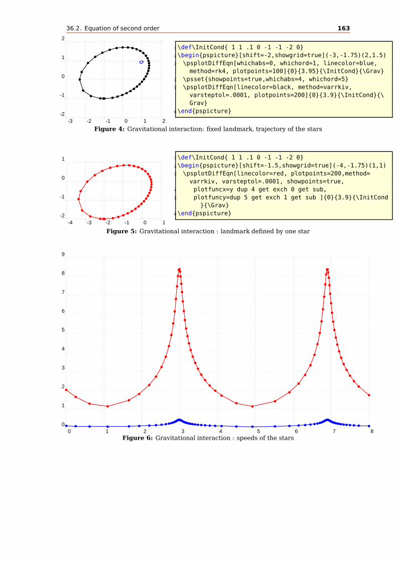
36.2. Equation of second order 163
-3 -2 -1 0 1 2-2
-1
0
1
2
bbbb
b
b
b
b
bb
b b b b b b bbbbbbbbbbbbbb
bb
bb
bbbb
1\def\InitCond{ 1 1 .1 0 -1 -1 -2 0}
2\begin{pspicture}[shift=-2,showgrid=true](-3,-1.75)(2,1.5)
3 \psplotDiffEqn[whichabs=0, whichord=1, linecolor=blue,
method=rk4, plotpoints=100]{0}{3.95}{\InitCond}{\Grav}
4 \psset{showpoints=true,whichabs=4, whichord=5}
5 \psplotDiffEqn[linecolor=black, method=varrkiv,
varsteptol=.0001, plotpoints=200]{0}{3.9}{\InitCond}{\
Grav}
6\end{pspicture}
Figure 4: Gravitational interaction: fixed landmark, trajectory of the stars
-4 -3 -2 -1 0 1-2
-1
0
1
bbbb
b
b
b
b
bb
b b b b b b bbbbbbbbbbbbb
bb
bb
bbbbb
1\def\InitCond{ 1 1 .1 0 -1 -1 -2 0}
2\begin{pspicture}[shift=-1.5,showgrid=true](-4,-1.75)(1,1)
3 \psplotDiffEqn[linecolor=red, plotpoints=200,method=
varrkiv, varsteptol=.0001, showpoints=true,
4 plotfuncx=y dup 4 get exch 0 get sub,
5 plotfuncy=dup 5 get exch 1 get sub ]{0}{3.9}{\InitCond
}{\Grav}
6\end{pspicture}
Figure 5: Gravitational interaction : landmark defined by one star
0 1 2 3 4 5 6 7 80
1
2
3
4
5
6
7
8
9
b
b
bb
b
b
b
b
b
b
b
b
b
b
b
b
b
b b b
b
b
b
b
b
b
b
b
b
b
b
b
b
b
b
b
b
b
bb
b
b
b
b
b
b
b
b
b
b
b
b
b
b bb
b
b
b
b
b
b
b
b
b
b
b
b
b
b
b
b
b
b b b b b b b b b b b b bb b b bb b b b b b b b b b b b b b b b b b b b b b b b b b b b b b b b
b b b bb b b b b b b b b b b b b b b b b b b b
Figure 6: Gravitational interaction : speeds of the stars
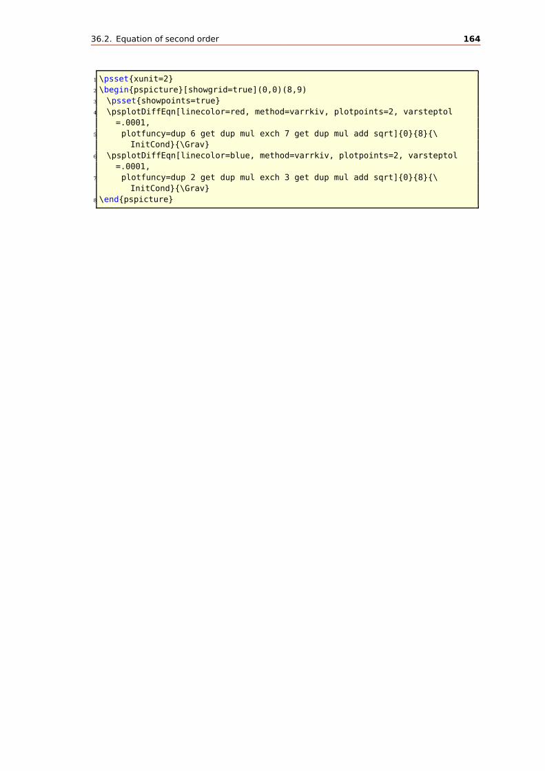
36.2. Equation of second order 164
1 \psset{xunit=2}
2 \begin{pspicture}[showgrid=true](0,0)(8,9)
3 \psset{showpoints=true}
4 \psplotDiffEqn[linecolor=red, method=varrkiv, plotpoints=2, varsteptol
=.0001,
5 plotfuncy=dup 6 get dup mul exch 7 get dup mul add sqrt]{0}{8}{\
InitCond}{\Grav}
6 \psplotDiffEqn[linecolor=blue, method=varrkiv, plotpoints=2, varsteptol
=.0001,
7 plotfuncy=dup 2 get dup mul exch 3 get dup mul add sqrt]{0}{8}{\
InitCond}{\Grav}
8 \end{pspicture}
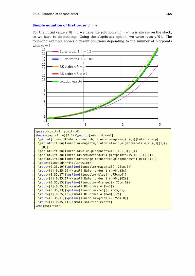
36.2. Equation of second order 165
Simple equation of first order y′ = y
For the initial value y(0) = 1 we have the solution y(x) = ex. y is always on the stack,
so we have to do nothing. Using the algebraic option, we write it as y[0]. The
following example shows different solutions depending to the number of plotpoints
with y0 = 1:
0 1 2 30123456789
10111213141516171819
Euler order 1 h = 0,2
Euler order 1 h = 0,02
RK ordre 4 h = 1
RK ordre 4 h = 0,2
solution exacte
1 \psset{xunit=4, yunit=.4}
2 \begin{pspicture}(3,19)\psgrid[subgriddiv=1]
3 \psplot[linewidth=6\pslinewidth, linecolor=green]{0}{3}{Euler x exp}
4 \psplotDiffEqn[linecolor=magenta,plotpoints=16,algebraic=true]{0}{3}{1}{y
[0]}
5 \psplotDiffEqn[linecolor=blue,plotpoints=151]{0}{3}{1}{}
6 \psplotDiffEqn[linecolor=red,method=rk4,plotpoints=15]{0}{3}{1}{}
7 \psplotDiffEqn[linecolor=Orange,method=rk4,plotpoints=4]{0}{3}{1}{}
8 \psset{linewidth=4\pslinewidth}
9 \rput*(0.35,19){\psline[linecolor=magenta](-.75cm,0)}
10 \rput*[l](0.35,19){\small Euler order 1 $h=0{,}2$}
11 \rput*(0.35,17){\psline[linecolor=blue](-.75cm,0)}
12 \rput*[l](0.35,17){\small Euler order 1 $h=0{,}02$}
13 \rput*(0.35,15){\psline[linecolor=Orange](-.75cm,0)}
14 \rput*[l](0.35,15){\small RK ordre 4 $h=1$}
15 \rput*(0.35,13){\psline[linecolor=red](-.75cm,0)}
16 \rput*[l](0.35,13){\small RK ordre 4 $h=0{,}2$}
17 \rput*(0.35,11){\psline[linecolor=green](-.75cm,0)}
18 \rput*[l](0.35,11){\small solution exacte}
19 \end{pspicture}
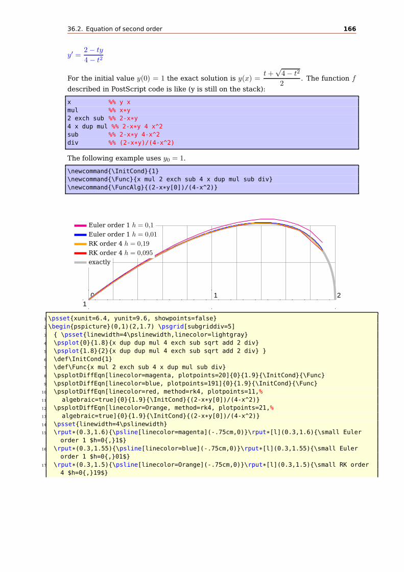
36.2. Equation of second order 166
y′ =2 − ty
4 − t2
For the initial value y(0) = 1 the exact solution is y(x) =t +
√4 − t2
2. The function f
described in PostScript code is like (y is still on the stack):
x %% y x
mul %% x*y
2 exch sub %% 2-x*y
4 x dup mul %% 2-x*y 4 x^2
sub %% 2-x*y 4-x^2
div %% (2-x*y)/(4-x^2)
The following example uses y0 = 1.
\newcommand{\InitCond}{1}
\newcommand{\Func}{x mul 2 exch sub 4 x dup mul sub div}
\newcommand{\FuncAlg}{(2-x*y[0])/(4-x^2)}
0 1 21
Euler order 1 h = 0,1
Euler order 1 h = 0,01
RK order 4 h = 0,19
RK order 4 h = 0,095
exactly
1 \psset{xunit=6.4, yunit=9.6, showpoints=false}
2 \begin{pspicture}(0,1)(2,1.7) \psgrid[subgriddiv=5]
3 { \psset{linewidth=4\pslinewidth,linecolor=lightgray}
4 \psplot{0}{1.8}{x dup dup mul 4 exch sub sqrt add 2 div}
5 \psplot{1.8}{2}{x dup dup mul 4 exch sub sqrt add 2 div} }
6 \def\InitCond{1}
7 \def\Func{x mul 2 exch sub 4 x dup mul sub div}
8 \psplotDiffEqn[linecolor=magenta, plotpoints=20]{0}{1.9}{\InitCond}{\Func}
9 \psplotDiffEqn[linecolor=blue, plotpoints=191]{0}{1.9}{\InitCond}{\Func}
10 \psplotDiffEqn[linecolor=red, method=rk4, plotpoints=11,%
11 algebraic=true]{0}{1.9}{\InitCond}{(2-x*y[0])/(4-x^2)}
12 \psplotDiffEqn[linecolor=Orange, method=rk4, plotpoints=21,%
13 algebraic=true]{0}{1.9}{\InitCond}{(2-x*y[0])/(4-x^2)}
14 \psset{linewidth=4\pslinewidth}
15 \rput*(0.3,1.6){\psline[linecolor=magenta](-.75cm,0)}\rput*[l](0.3,1.6){\small Euler
order 1 $h=0{,}1$}
16 \rput*(0.3,1.55){\psline[linecolor=blue](-.75cm,0)}\rput*[l](0.3,1.55){\small Euler
order 1 $h=0{,}01$}
17 \rput*(0.3,1.5){\psline[linecolor=Orange](-.75cm,0)}\rput*[l](0.3,1.5){\small RK order
4 $h=0{,}19$}
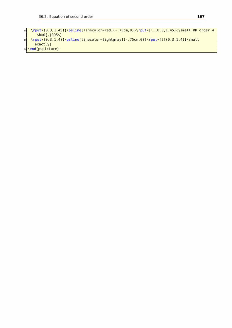
36.2. Equation of second order 167
18 \rput*(0.3,1.45){\psline[linecolor=red](-.75cm,0)}\rput*[l](0.3,1.45){\small RK order 4
$h=0{,}095$}
19 \rput*(0.3,1.4){\psline[linecolor=lightgray](-.75cm,0)}\rput*[l](0.3,1.4){\small
exactly}
20 \end{pspicture}
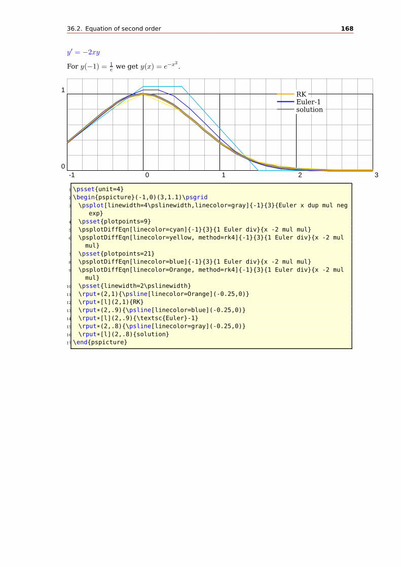
36.2. Equation of second order 168
y′ = −2xy
For y(−1) = 1ewe get y(x) = e−x2
.
-1 0 1 2 30
1RKEuler-1solution
1 \psset{unit=4}
2 \begin{pspicture}(-1,0)(3,1.1)\psgrid
3 \psplot[linewidth=4\pslinewidth,linecolor=gray]{-1}{3}{Euler x dup mul neg
exp}
4 \psset{plotpoints=9}
5 \psplotDiffEqn[linecolor=cyan]{-1}{3}{1 Euler div}{x -2 mul mul}
6 \psplotDiffEqn[linecolor=yellow, method=rk4]{-1}{3}{1 Euler div}{x -2 mul
mul}
7 \psset{plotpoints=21}
8 \psplotDiffEqn[linecolor=blue]{-1}{3}{1 Euler div}{x -2 mul mul}
9 \psplotDiffEqn[linecolor=Orange, method=rk4]{-1}{3}{1 Euler div}{x -2 mul
mul}
10 \psset{linewidth=2\pslinewidth}
11 \rput*(2,1){\psline[linecolor=Orange](-0.25,0)}
12 \rput*[l](2,1){RK}
13 \rput*(2,.9){\psline[linecolor=blue](-0.25,0)}
14 \rput*[l](2,.9){\textsc{Euler}-1}
15 \rput*(2,.8){\psline[linecolor=gray](-0.25,0)}
16 \rput*[l](2,.8){solution}
17 \end{pspicture}

36.2. Equation of second order 169
Spiral of Cornu
The integrals of Fresnel:
x =
∫ t
0cos
πt2
2dt (2)
y =
∫ t
0sin
πt2
2dt (3)
with
x = cosπt2
2(4)
y = sinπt2
2(5)
1 \psset{unit=8}
2 \begin{pspicture}(1,1)\psgrid[subgriddiv=5]
3 \psplotDiffEqn[whichabs=0,whichord=1,linecolor=red,method=rk4,algebraic,%
4 plotpoints=500,showpoints=true]{0}{10}{0 0}{cos(Pi*x^2/2)|sin(Pi*x^2/2)}
5 \end{pspicture}
0 10
1
b b b b b b b b b b b b b b bb b b b
b b bb b
b bb b
b bb b
bbbbbbbbbbbbbbbbbbbbbbbbbbbbbbbbb
bbbbbbbbbbbbb
bbbbbbbbbbbbbbbbbb b b b b b b b
b bbbbbbbbbbbbbbbb
bbbbbbbbbbbbbbbbbbb b b b b b
b bbbbbbbbbb
bbbbbbb
bbbbbbbbb b b b b b
bbbbbbbbbb
bbbbbbbbbbbb b b b b
bbbbbbbbb
bbbbbbbbbbb b b b b
bbbbbbbb
bbbbbbbbb b b b b
bbbbbbb
bbbbbbbbb b b b
bbbbbbb
bbbbbbbbb b b b
bbbbbb
bbbbbbbb b b b
bbbbbbbbb
bbbb b b b
bbbbbbbb
bbbb b b b
bbbbbbbb
bbbb b b b
bbbbb
bbbbbb b b b
bbbbb
bbbbbb b b b
bbbbbb
bbbb b b b
bbbbbb
bbbb b b
bbbbbbb
bbb b b b
bbbbbb
bbb b b
bbbbbbb
bbb b b
bbbbbb
bbb b b
bbbbbb
bbb b b
bbbbbb
bbb b b
bbbbbb
bbb b b
bbbbb
bbb b b
bbbbb
bbb b

36.2. Equation of second order 170
Lotka-Volterra
The Lotka-Volterra model describes interactions between two species in an ecosystem,
a predator and a prey. This represents our first multi-species model. Since we are
considering two species, the model will involve two equations, one which describes
how the prey population changes and the second which describes how the predator
population changes.
For concreteness let us assume that the prey in our model are rabbits, and that the
predators are foxes. If we let R(t) and F (t) represent the number of rabbits and foxes,
respectively, that are alive at time t, then the Lotka-Volterra model is:
R = a · R − b · R · F (6)
F = e · b · R · F − c · F (7)
where the parameters are defined by:
a is the natural growth rate of rabbits in the absence of predation,
c is the natural death rate of foxes in the absence of food (rabbits),
b is the death rate per encounter of rabbits due to predation,
e is the efficiency of turning predated rabbits into foxes.
The Stella model representing the Lotka-Volterra model will be slightly more com-
plex than the single species models we’ve dealt with before. The main difference is
that our model will have two stocks (reservoirs), one for each species. Each species
will have its own birth and death rates. In addition, the Lotka-Volterra model involves
four parameters rather than two. All told, the Stella representation of the Lotka-
Volterra model will use two stocks, four flows, four converters and many connectors.
-3 -2 -1 0 1 2 3 4 5 6 7 8 9 10-3
-2
-1
0
1
2
3
4
5
6
7
8
9
10
bbbbbbbbbbbbbbbbbbbb
b
b
b
b
b
b
b
b
b
b
b
b
b
b
bbbbbb
b
b
b
b
b
b
b
b
b
b
b
b
b
b
bb
b
b
b
b

36.2. Equation of second order 171
1 \def\InitCond{ 0 10 10}%% xa ya xl
2 \def\Faiglelapin{\Vaigle*(y[2]-y[0])/sqrt(y[1]^2+(y[2]-y[0])^2)|%
3 -\Vaigle*y[1]/sqrt(y[1]^2+(y[2]-y[0])^2)|%
4 -\Vlapin}
5 \def\Vlapin{1} \def\Vaigle{1.6}
6 \psset{unit=.7,subgriddiv=0,gridcolor=lightgray,method=adams,algebraic,%
7 plotpoints=20,showpoints=true}
8 \begin{pspicture}[showgrid=true](-3,-3)(10,10)
9 \psplotDiffEqn[plotfuncy=pop 0,whichabs=2,linecolor=red]{0}{10}{\InitCond}{\
Faiglelapin}
10 \psplotDiffEqn[whichabs=0,whichord=1,linecolor=black,method=rk4]{0}{10}{\InitCond}{\
Faiglelapin}
11 \psplotDiffEqn[whichabs=0,whichord=1,linecolor=blue]{0}{10}{\InitCond}{\Faiglelapin
}
12 \end{pspicture}
0 1 2 3 4 5 6 7 8 9 100
1
2
3
4
5
6
7
8
9
10
11
12
13
14 b
b
b
b
b
b
b
b
b
b
b
b
b
b
bb b b b b
b
b
b
b
b
b
b
b
b
b
b
b
b
b
bb
b
b
b
b
b b b b b b b b b b b b b b b b b b b b
1 \def\InitCond{ 0 10 10}%% xa ya xl
2 \def\Faiglelapin{\Vaigle*(y[2]-y[0])/sqrt(y[1]^2+(y[2]-y[0])^2)|%
3 -\Vaigle*y[1]/sqrt(y[1]^2+(y[2]-y[0])^2)|%
4 -\Vlapin}
5 \def\Vlapin{1} \def\Vaigle{1.6}
6 \psset{unit=.7,subgriddiv=0,gridcolor=lightgray,method=adams,algebraic,%
7 plotpoints=20,showpoints=true}
8 \begin{pspicture}[showgrid=true](10,12)
9 \psplotDiffEqn[plotfuncy=dup 1 get dup mul exch dup 0 get exch 2 get sub dup
10 mul add sqrt,linecolor=red,method=rk4]{0}{10}{\InitCond}{\Faiglelapin}

36.2. Equation of second order 172
11 \psplotDiffEqn[plotfuncy=dup 1 get dup mul exch dup 0 get exch 2 get sub dup
12 mul add sqrt,linecolor=blue]{0}{10}{\InitCond}{\Faiglelapin}
13 \psplotDiffEqn[plotfuncy=pop Func aload pop pop dup mul exch dup mul add sqrt,
14 linecolor=yellow]{0}{10}{\InitCond}{\Faiglelapin}
15 \end{pspicture}
y′′ = y
Beginning with the initial equation y(x) = Aex + Be−x we get the hyperbolic trigono-
metrical functions.
0 1 20
1
2
3
4
5
6
7
Euler order 1 h = 1Euler order 1 h = 0,1RK order 4 h = 1exact solution
1 \def\Funct{exch} \psset{xunit=5cm, yunit=0.75cm}
2 \begin{pspicture}(0,-0.25)(2,7)\psgrid[subgriddiv=1,griddots=10]
3 \psplot[linewidth=4\pslinewidth, linecolor=green]{0}{2}{Euler x exp} %%e^x
4 \psplotDiffEqn[linecolor=magenta, plotpoints=11]{0}{2}{1 1}{\Funct}
5 \psplotDiffEqn[linecolor=blue, plotpoints=101]{0}{2}{1 1}{\Funct}
6 \psplotDiffEqn[linecolor=red, method=rk4, plotpoints=11]{0}{2}{1 1}{\Funct}
7 \psplot[linewidth=4\pslinewidth, linecolor=green]{0}{2}{Euler dup x exp %%ch(x)
8 exch x neg exp add 2 div}
9 \psplotDiffEqn[linecolor=magenta, plotpoints=11]{0}{2}{1 0}{\Funct}
10 \psplotDiffEqn[linecolor=blue, plotpoints=101]{0}{2}{1 0}{\Funct}
11 \psplotDiffEqn[linecolor=red, method=rk4, plotpoints=11]{0}{2}{1 0}{\Funct}
12 \psplot[linewidth=4\pslinewidth, linecolor=green]{0}{2}{Euler dup x exp
13 exch x neg exp sub 2 div} %%sh(x)
14 \psplotDiffEqn[linecolor=magenta, plotpoints=11]{0}{2}{0 1}{\Funct}
15 \psplotDiffEqn[linecolor=blue, plotpoints=101]{0}{2}{0 1}{\Funct}
16 \psplotDiffEqn[linecolor=red, method=rk4, plotpoints=11]{0}{2}{0 1}{\Funct}
17 \rput*(1.3,.9){\psline[linecolor=magenta](-.75cm,0)}\rput*[l](1.3,.9){\small\textsc{
Euler} order 1 $h=1$}
18 \rput*(1.3,.8){\psline[linecolor=blue](-.75cm,0)}\rput*[l](1.3,.8){\small\textsc{
Euler} order 1 $h=0{,}1$}
19 \rput*(1.3,.7){\psline[linecolor=red](-.75cm,0)}\rput*[l](1.3,.7){\small RK order 4
$h=1$}
20 \rput*(1.3,.6){\psline[linecolor=green](-.75cm,0)}\rput*[l](1.3,.6){\small exact
solution}
21 \end{pspicture}

36.2. Equation of second order 173
y′′ = −y
0 1 2 3 4 5 6 7 8 9 10 11 12 13-1
0
1
Euler order 1 h = 1Euler order 1 h = 0,1RK order 4 h = 1exact solution
1 \def\Funct{exch neg}
2 \psset{xunit=1, yunit=4}
3 \def\quatrepi{12.5663706144}%%4pi=12.5663706144
4 \begin{pspicture}(0,-1.25)(\quatrepi,1.25)\psgrid[subgriddiv=1,griddots=10]
5 \psplot[linewidth=4\pslinewidth,linecolor=green]{0}{\quatrepi}{x RadtoDeg
cos}%%cos(x)
6 \psplotDiffEqn[linecolor=blue, plotpoints=201]{0}{3.1415926}{1 0}{\Funct}
7 \psplotDiffEqn[linecolor=red, method=rk4, plotpoints=31]{0}{\quatrepi}{1
0}{\Funct}
8 \psplot[linewidth=4\pslinewidth,linecolor=green]{0}{\quatrepi}{x RadtoDeg
sin} %%sin(x)
9 \psplotDiffEqn[linecolor=blue,plotpoints=201]{0}{3.1415926}{0 1}{\Funct}
10 \psplotDiffEqn[linecolor=red,method=rk4, plotpoints=31]{0}{\quatrepi}{0
1}{\Funct}
11 \rput*(3.3,.9){\psline[linecolor=magenta](-.75cm,0)}\rput*[l](3.3,.9){\
small Euler order 1 $h=1$}
12 \rput*(3.3,.8){\psline[linecolor=blue](-.75cm,0)}\rput*[l](3.3,.8){\small
Euler order 1 $h=0{,}1$}
13 \rput*(3.3,.7){\psline[linecolor=red](-.75cm,0)}\rput*[l](3.3,.7){\small RK
order 4 $h=1$}
14 \rput*(3.3,.6){\psline[linecolor=green](-.75cm,0)}\rput*[l](3.3,.6){\small
exact solution}
15 \end{pspicture}

36.2. Equation of second order 174
The mechanical pendulum: y′′ = − glsin(y)
For small oscillations sin(y) ≃ y:
y(x) = y0 cos
(√g
lx
)
The function f is written in PostScript code:
exch RadtoDeg sin -9.8 mul %% y’ -gsin(y)
0
1
−1
−2
1 2
1 \def\Func{y[1]|-9.8*sin(y[0])}
2 \psset{yunit=2,xunit=4,algebraic=true,linewidth=1.5pt}
3 \begin{pspicture}(0,-2.25)(3,2.25)
4 \psaxes{->}(0,0)(0,-2)(3,2)
5 \psplot[linewidth=3\pslinewidth, linecolor=Orange]{0}{3}{.1*cos(sqrt(9.8)*x)}
6 \psset{method=rk4,plotpoints=50,linecolor=blue}
7 \psplotDiffEqn{0}{3}{.1 0}{\Func}
8 \psplot[linewidth=3\pslinewidth,linecolor=Orange]{0}{3}{.25*cos(sqrt(9.8)*x)}
9 \psplotDiffEqn{0}{3}{.25 0}{\Func}
10 \psplotDiffEqn{0}{3}{.5 0}{\Func}
11 \psplotDiffEqn{0}{3}{1 0}{\Func}
12 \psplotDiffEqn[plotpoints=100]{0}{3}{Pi 2 div 0}{\Func}
13 \end{pspicture}

36.2. Equation of second order 175
y′′ = −y′
4 − 2y
For y0 = 5 and y′
0 = 0 the solution is:
5e−x8
(
cos (ωx) +sin(ωx)
8ω
)
avec ω =
√127
8
0
1
2
3
4
−1
−2
−3
−4
1 2 3 4 5 6 7 8 9 10 11 12 13 14 15 16 17 18 19 20 21 22 23 24 25
1 \psset{xunit=.6,yunit=0.8,plotpoints=500}
2 \begin{pspicture}(0,-4.25)(26,5.25)
3 \psaxes{->}(0,0)(0,-4)(26,5)
4 \psplot[plotpoints=200,linewidth=4\pslinewidth,linecolor=gray]{0}{26}{%
5 Euler x -8 div exp x 127 sqrt 8 div mul RadtoDeg dup cos 5 mul exch sin
127 sqrt div 5 mul add mul}
6 \psplotDiffEqn[linecolor=red,linewidth=5\pslinewidth]{0}{26}{5 0}
7 {dup 3 1 roll -4 div exch 2 mul sub}
8 \psplotDiffEqn[linecolor=black,algebraic]{0}{26}{5 0} {y[1]|-y[1]/4-2*y
[0]}
9 \psset{method=rk4, plotpoints=50}
10 \psplotDiffEqn[linecolor=blue,linewidth=5\pslinewidth]{0}{26}{5 0}{%
11 dup 3 1 roll -4 div exch 2 mul sub}
12 \psplotDiffEqn[linecolor=black,algebraic=true]{0}{26}{5 0}{y[1]|-y[1]/4-2*y[0]}
13 \end{pspicture}

37. \psBoxplot 176
37. \psBoxplot
A box-and-whisker plot (often called simply a box plot) is a histogram-like method of
displaying data, invented by John.Tukey. The box-and-whisker plot is a box with ends
at the quartiles Q1 and Q3 and has a statistical median M as a horizontal line in the
box. The "‘whiskers"* are lines to the farthest points that are not outliers (i.e., that
are within 3/2 times the interquartile range of Q1 and Q3). Then, for every point more
than 3/2 times the interquartile range from the end of a box, is a dot.
The only special optional arguments, beside all other which are valid for drawing
lines and filling areas, are IQLfactor, barwidth, and arrowlength, where the latter
is a factor which is multiplied with the barwidth for the line ends. The IQLfactor,
preset to 1.5, defines the area for the outliers.
20012008
2001 2008
20012008
0
10
20
30
40
50
60
70
80
90
100
110
120
130
0 1 2 3 4 5 6 7 8 9 10 11 12
1 \begin{pspicture}(-1,-1)(12,14)
2 \psset{yunit=0.1,fillstyle=solid}
3 \savedata{\data}[100 90 120 115 120 110 100 110 100 90 100 100 120 120 120]

37. \psBoxplot 177
4 \rput(1,0){\psBoxplot[fillcolor=red!30]{\data}}
5 \rput(1,105){2001}
6 \savedata{\data}[90 120 115 116 115 110 90 130 120 120 120 85 100 130 130]
7 \rput(3,0){\psBoxplot[arrowlength=0.5,fillcolor=blue!30]{\data}}
8 \rput(3,107){2008}
9 \savedata{\data}[35 70 90 60 100 60 60 80 80 60 50 55 90 70 70]
10 \rput(5,0){\psBoxplot[barwidth=40pt,arrowlength=1.2,fillcolor=red!30]{\data
}}
11 \rput(5,65){2001}
12 \savedata{\data}[60 65 60 75 75 60 50 90 95 60 65 45 45 60 90]
13 \rput(7,0){\psBoxplot[barwidth=40pt,fillcolor=blue!30]{\data}}
14 \rput(7,65){2008}
15 \savedata{\data}[20 20 25 20 15 20 20 25 30 20 20 20 30 30 30]
16 \rput(9,0){\psBoxplot[fillcolor=red!30]{\data}}
17 \rput(9,22){2001}
18 \savedata{\data}[20 30 20 35 35 20 20 60 50 20 35 15 30 20 40]
19 \rput(11,0){\psBoxplot[fillcolor=blue!30,linestyle=dashed]{\data}}
20 \rput(11,25){2008}
21 \psaxes[dy=1cm,Dy=10](0,0)(12,130)
22 \end{pspicture}
The next example uses an external file for the data, which must first be read by the
macro \readdata. The next one creates a horizontal boxplot by rotating the output
with −90 degrees.
0
4
8
12
16
20
24
28
32
0 1 20
1
2
0 4 8 12 16 20 24 28 32
1 \readdata{\data}{boxplot.data}
2 \begin{pspicture}(-1,-1)(2,10)

37. \psBoxplot 178
3 \psset{yunit=0.25,fillstyle=solid}
4 \savedata{\data}[2 4 6 8 10 12 14 16 18 20 22 24 26 28 30 32]
5 \rput(1,0){\psBoxplot[fillcolor=blue!30]{\data}}
6 \psaxes[dy=1cm,Dy=4](0,0)(2,35)
7 \end{pspicture}
8 %
9 \begin{pspicture}(-1,-1)(11,2)
10 \psset{xunit=0.25,fillstyle=solid}
11 \savedata{\data}[2 4 6 8 10 12 14 16 18 20 22 24 26 28 30 32]
12 \rput{-90}(0,1){\psBoxplot[yunit=0.25,fillcolor=blue!30]{\data}}
13 \psaxes[dx=1cm,Dx=4](0,0)(35,2)
14 \end{pspicture}

38. \psMatrixPlot 179
38. \psMatrixPlot
This macro allows you to visualize a matrix. The datafile must be defined as a PostScript
matrix named dotmatrix:
/dotmatrix [ % <------------ important line
0 1 1 0 0 0 0 1 1 1
0 1 1 0 1 1 1 0 1 0
1 0 1 1 0 0 0 1 1 0
0 0 1 0 0 0 0 0 1 1
1 1 1 1 1 0 1 0 0 1
0 0 1 1 0 1 0 1 1 1
1 0 0 0 1 1 0 0 0 1
0 0 0 1 1 1 0 1 1 0
1 1 0 0 0 0 1 0 0 1
1 0 1 0 0 1 1 1 0 0
] def % <------------ important line
Only the value 0 is important, in which case nothing happens, and for all other cases
a dot is printed. The syntax of the macro is:
\psMatrixPlot [Options] {rows}{columns}{data file}
The matrix is scanned line by line from the the first one to the last. In general it ap-
pears as a bottom-to-top version of the above listed matrix, the first row 0 1 1 0 0 0 0 1 1 1is the first plotted line (y = 1). With the option ChangeOrder=true it looks exactly
like the above view.

38. \psMatrixPlot 180
0
1
2
3
4
5
6
7
8
9
10
0 1 2 3 4 5 6 7 8 9 10
r r r r rr r r r r rr r r r rr r r
r r r r r r rr r r r r r
r r r rr r r r r
r r r rr r r r rbc bc bc bc bc
bc bc bc bc bc bc
bc bc bc bc bc
bc bc bc
bc bc bc bc bc bc bc
bc bc bc bc bc bc
bc bc bc bc
bc bc bc bc bc
bc bc bc bc
bc bc bc bc bc
1 \begin{pspicture}(-0.5,-0.75)(11,11)
2 \psaxes{->}(11,11)
3 \psMatrixPlot[dotsize=1.1cm,dotstyle=square*,linecolor=magenta]%
4 {10}{10}{matrix.data}
5 \psMatrixPlot[dotsize=.5cm,dotstyle=o,ChangeOrder]{10}{10}{matrix.data}
6 \end{pspicture}

38. \psMatrixPlot 181
0
1
2
3
4
5
6
7
8
9
10
0 1 2 3 4 5 6 7 8 9 10
b b b
b b b b b b
b b b b b
b b
b b b
b b b b b b
b b b b
b b b b
b b b
b b b b b
1\begin{pspicture}(-0.5,-0.75)(11,11)
2 \psaxes{->}(11,11)
3 \psMatrixPlot[dotscale=3,dotstyle=*,linecolor=blue]{10}{8}{matrix.data}
4\end{pspicture}

39. \psforeach and \psForeach 182
39. \psforeach and \psForeach
The macro \psforeach allows a loop with an individual increment.
\psforeach{variable}{value list}{action}
\psForeach{variable}{value list}{action}
With \psforeach the action is done inside a group and for \psForeach not. This
maybe useful when using the macro to create tabular cells, which are alread grouped
itself.
0 1 2 3 4 50
1
2
3
4
5
b
bb
b
b
1\begin{pspicture}[showgrid=true
](5,5)
2 \psforeach{\nA}{0, 1, 1.5, 3, 5}{
%
3 \psdot[dotscale=3](\nA,\nA)}
4\end{pspicture}
y = 2x
2 4 6 8 10 12
4.0 16.0 64.0 256.0 1024.0 4096.0
1%\usepackage{pst-func}
2\makeatletter
3\newcommand*\InitToks{\toks@={}}
4\newcommand\AddToks[1]{\toks@=\expandafter{\the\toks@ #1}}
5\newcommand*\PrintToks{\the\toks@}
6\newcommand*{\makeTable}[4][5mm]{%
7 \begingroup
8 \InitToks%
9 \AddToks{\begin{tabular}{|*{#2}{>{\RaggedLeft}p{#1}|}@{}l@{}}\cline
{1-#2}}
10 \psForeach{\iA}{#3}{\expandafter\AddToks\expandafter{\iA & }}
11 \AddToks{\\\cline{1-#2}}%
12 \psForeach{\iA}{#3}{\expandafter\AddToks\expandafter{\expandafter%
13 \psPrintValue\expandafter{\iA\space /x ED #4} & }}
14 \AddToks{\\\cline{1-#2}\end{tabular}}%
15 \PrintToks
16 \endgroup
17}
18\makeatother
19
20\sffamily
21\psset{decimals=2,valuewidth=7,xShift=-20}
22$y=2^x$\\
23\makeTable[1cm]{6}{2,4,6,8,10,12}{2 x exp}

40. \resetOptions 183
40. \resetOptions
Sometimes it is difficult to know what options, which are changed inside a long doc-
ument, are different to the default ones. With this macro all options belonging to
pst-plot can be reset. This refers to all options of the packages pstricks, pst-plot
and pst-node.
A. PostScript
PostScript uses the stack system and the LIFO system, "’Last In, First Out"‘.
Table 5: Some primitive PostScript macros
FunctionMeaning
on stack before → after
add x y → x + ysub x y → x − ymul x y → x × ydiv x y → x ÷ ysqrt x → √
xabs x → |x|neg x → −xcos x → cos(x) (x in degrees)
sin x → sin(x) (x in degrees)
tan x → tan(x) (x in degrees)
atan y x → ∠( ~Ox; ~OM) (in degrees of M(x, y))ln x → ln(x)log x → log(x)array n → v (of dimension n)aload v → x1 x2 · · · xn vastore x1 x2 · · · xn v → [v]pop x → -
dup x → x x

B. List of all optional arguments for pstricks-add 184
B. List of all optional arguments for pstricks-add
Key Type Default
CMYK boolean true
fsAngle ordinary 137.50775
fsOrigin ordinary [none]
maxdashes ordinary 11
intSeparator ordinary [none]
braceWidth ordinary [none]
bracePos ordinary [none]
braceWidthInner ordinary [none]
braceWidthOuter ordinary [none]
veearrowlength ordinary 3mm
veearrowangle ordinary 30
veearrowlinewidth ordinary 0.35mm
filledveearrowlength ordinary 3mm
filledveearrowangle ordinary 15
filledveearrowlinewidth ordinary 0.35mm
arrowLW ordinary [none]
tickarrowlength ordinary 1.5mm
tickarrowlinewidth ordinary 0.35mm
hooklength ordinary 3mm
hookwidth ordinary 1mm
ArrowFill boolean true
nArrowsA ordinary 2
nArrowsB ordinary 2
nArrows ordinary 2
ArrowInside ordinary [none]
ArrowInsidePos ordinary 0.5
ArrowInsideNo ordinary 1
ArrowInsideOffset ordinary 0
dashNo ordinary [none]
linecap ordinary [none]
randomPoints ordinary 1000
color boolean true
lineAngle ordinary 0
trueAngle boolean true
blName command
bcName command
brName command
clName command
ccName command
crName command
tlName command
tcName command
Continued on next page

B. List of all optional arguments for pstricks-add 185
Continued from previous page
Key Type Default
trName command
yMaxValue ordinary -1.0
labelFontSize ordinary
mathLabel boolean true
decimalSeparator ordinary .
comma boolean true
xAxis boolean true
yAxis boolean true
xyAxes boolean true
xlabelPos ordinary b
ylabelPos ordinary l
xyDecimals ordinary
xDecimals ordinary
yDecimals ordinary
xlogBase ordinary
ylogBase ordinary
xylogBase ordinary
trigLabelBase ordinary 0
trigLabelsSimplify boolean true
trigLabels boolean true
logLines ordinary none
ylabelFactor ordinary \relax
xlabelFactor ordinary \relax
showOriginTick boolean true
xticksize ordinary [none]
yticksize ordinary [none]
subticks ordinary 1
xsubticks ordinary 1
ysubticks ordinary 1
subticksize ordinary 0.75
xsubticksize ordinary 0.75
ysubticksize ordinary 0.75
tickwidth ordinary 0.5\pslinewidth
xtickwidth ordinary 0.5\pslinewidth
ytickwidth ordinary 0.5\pslinewidth
subtickwidth ordinary 0.25\pslinewidth
xsubtickwidth ordinary 0.25\pslinewidth
ysubtickwidth ordinary 0.25\pslinewidth
tickcolor ordinary black
xtickcolor ordinary black
ytickcolor ordinary black
subtickcolor ordinary gray
xsubtickcolor ordinary gray
ysubtickcolor ordinary gray
Continued on next page

B. List of all optional arguments for pstricks-add 186
Continued from previous page
Key Type Default
xticklinestyle ordinary solid
xsubticklinestyle ordinary solid
yticklinestyle ordinary solid
ysubticklinestyle ordinary solid
ticklinestyle ordinary solid
subticklinestyle ordinary solid
nStep ordinary 1
nStart ordinary 0
nEnd ordinary
xStep ordinary 0
yStep ordinary 0
xStart ordinary
xEnd ordinary
yStart ordinary
yEnd ordinary
plotNo ordinary 1
plotNoMax ordinary 1
xyValues boolean true
ChangeOrder boolean true
xAxisLabel ordinary x
yAxisLabel ordinary y
xAxisLabelPos ordinary
yAxisLabelPos ordinary
llx ordinary \z@
lly ordinary \z@
urx ordinary \z@
ury ordinary \z@
box ordinary true
ignoreLines ordinary [none]
polarplot boolean true
algebraic boolean true
method ordinary [none]
whichabs ordinary [none]
whichord ordinary [none]
plotfuncx ordinary [none]
plotfuncy ordinary [none]
expression ordinary [none]
buildvector boolean true
VarStep boolean true
PlotDerivative ordinary [none]
VarStepEpsilon ordinary [none]
varsteptol ordinary [none]
adamsorder ordinary [none]
barwidth ordinary [none]
Continued on next page

References 187
Continued from previous page
Key Type Default
PSfont ordinary Times-Roman
valuewidth ordinary 10
fontscale ordinary 10
decimals ordinary -1
StepType ordinary [none]
Derive ordinary [none]
Tnormal boolean true
filename ordinary [none]
saveData boolean true
IQLfactor ordinary [none]
chartStyle ordinary [none]
chartColor ordinary [none]
chartSep ordinary [none]
chartStack ordinary [none]
chartStackDepth ordinary [none]
chartStackWidth ordinary [none]
chartHeight ordinary [none]
userColor ordinary [none]
chartNodeI ordinary [none]
chartNodeO ordinary [none]
References
[1] Hendri Adriaens. xkeyval package. CTAN:/macros/latex/contrib/xkeyval,
2004.
[2] Denis Girou. Présentation de PSTricks. Cahier GUTenberg, 16:21–70, April
1994.
[3] Michel Goosens, Frank Mittelbach, Sebastian Rahtz, Denis Roegel, and Herbert
Voß. The LATEX Graphics Companion. Addison-Wesley Publishing Company,
Reading, Mass., 2007.
[4] Alan Hoenig. TEX Unbound: LATEX & TEX Strategies, Fonts, Graphics, and More.
Oxford University Press, London, 1998.
[5] Laura E. Jackson and Herbert Voß. Die plot-funktionen von pst-plot. Die
TEXnische Komödie, 2/02:27–34, June 2002.
[6] Nikolai G. Kollock. PostScript richtig eingesetzt: vom Konzept zum praktischen
Einsatz. IWT, Vaterstetten, 1989.
[7] Frank Mittelbach and Michel Goosens et al. The LATEX Companion. Addison-
Wesley Publishing Company, Boston, second edition, 2004.
[8] Frank Mittelbach and Michel Goosens et al. Der LATEX Begleiter. Pearson Edu-
cation, München, zweite edition, 2005.
References 188
[9] Herbert Voß. Chaos und Fraktale selbst programmieren: von Mandelbrotmen-
gen über Farbmanipulationen zur perfekten Darstellung. Franzis Verlag, Poing,
1994.
[10] Herbert Voß. Die mathematischen Funktionen von PostScript. Die TEXnische
Komödie, 1/02, March 2002.
[11] Herbert Voß. PSTricks Grafik für TEX und LATEX. DANTE – Lob.media, Heidel-
berg/Hamburg, fifth edition, 2008.
[12] Herbert Voß. Mathematiksatz in LATEX. Lehmanns Media/DANTE, Berlin/Hei-
delberg, first edition, 2009.
[13] Timothy Van Zandt. PSTricks - PostScript macros for generic TEX. http://
www.tug.org/application/PSTricks, 1993.
[14] Timothy Van Zandt. multido.tex - a loop macro, that supports fixed-point addi-
tion. CTAN:/graphics/pstricks/generic/multido.tex, 1997.
[15] Timothy Van Zandt. pst-plot: Plotting two dimensional functions and data.
CTAN:graphics/pstricks/generic/pst-plot.tex, 1999.
[16] Timothy Van Zandt and Denis Girou. Inside PSTricks. TUGboat, 15:239–246,
September 1994.

Index
Symbols
\hAmacroB, 9
(-), 28
)-(, 28
*, 39
**-**, 28
*-), 28
*-*, 28
-, 28
->, 28, 31
-dCompatibilityLevel, 41
-<<, 29
->>, 29
<-, 31
<->, 28
<<->>, 28
>-<, 28
[->, 28
[-], 28
]-[, 28
<<-, 29
<<-<<, 29
<<->>, 29
>>-, 29
>>-<<, 28, 29
>>->>, 29
A
abs, 183
add, 183
algebraic, 63, 95, 131, 134, 137, 139,
157, 165
all, 63
aload, 183
angle, 53
angleA, 52
angleB, 51
armA, 49, 50
armB, 49–51
array, 183
ArrowFill, 31
ArrowInside, 31
ArrowInsideNo, 31
ArrowInsideOffset, 31
ArrowInsidePos, 31
arrowlength, 176
arrowLW, 39, 40
arrows, 28
arrowscale, 39
astore, 183
atan, 183
axes, 63
axesstyle, 63
axis, 63, 67
B
B, 21
b, 21
barwidth, 99, 176
bottom, 62, 63, 78
brace, 20
bracePos, 20, 21
braceWidth, 20, 21
braceWidthInner, 21
braceWidthOuter, 21
buildvector, 157
C
C, 21
c, 21, 129
\cancel, 121
cardioid, 136
ChangeOrder, 64, 104, 113, 179
chartColor, 16
chartFillColor?, 16
chartNodeI, 16
chartNodeO, 16
chartSep, 16
color, 25
comma, 62, 63, 70
cos, 183
curve, 106
D
dash, 10
dashed, 63
\dataplot, 104
decimalSeparator, 63, 70
default, 134, 141
189

Index 190
Derive, 134–136, 139
\displaystyle, 68
div, 183
Division, 7
dotmatrix, 179
dots, 105
dotted, 63
dup, 183
dx, 74
Dy, 65
E
\endpsgraph, 123
Environment
– psgraph, 123
– pspicture, 53, 54, 120, 129
F
false, 31
\fileplot, 104
fillcolor, 21
filledveearrowangle, 39
filledveearrowlength, 39
filledveearrowlinewidth, 39
fillstyle
– eofill, 2
floating point, 7
frame, 63, 77
Fresnel, 169
full, 62, 63
G
Gouraud, 44
H
H, 30
hooklength, 30
hookwidth, 30
hydrogen, 43
I
i, 131
IfTE, 98
ignoreLines, 64, 104
infimum, 131
inner, 62, 63, 77
InsideArrow, 2
intSeparator, 41
IQLfactor, 176
K
Keyvalue
– all, 63
– axes, 63
– axis, 63, 67
– B, 21
– b, 21
– bottom, 62, 63
– C, 21
– c, 21
– curve, 106
– dashed, 63
– default, 141
– dotted, 63
– frame, 63, 77
– full, 63
– i, 131
– infimum, 131
– inner, 62, 63, 77
– l, 21
– left, 63
– line, 104
– LSM, 114
– none, 63, 82
– polar, 63, 65
– R, 131
– r, 21
– Riemann, 131
– right, 63
– s, 131
– solid, 63
– supremum, 131
– t, 21
– top, 62, 63
– u, 131
– upper, 131
– x, 63
– y, 63
Keyword
– algebraic, 63, 95, 131, 134, 137, 139,
157, 165
– angle, 53
– angleA, 52
– angleB, 51
– armA, 49, 50

Index 191
– armB, 49–51
– ArrowFill, 31
– ArrowInside, 31
– ArrowInsideNo, 31
– ArrowInsideOffset, 31
– ArrowInsidePos, 31
– arrowlength, 176
– arrowLW, 39, 40
– arrows, 28
– arrowscale, 39
– axesstyle, 63
– barwidth, 99, 176
– bracePos, 20, 21
– braceWidth, 20, 21
– braceWidthInner, 21
– braceWidthOuter, 21
– buildvector, 157
– ChangeOrder, 64, 104, 113, 179
– chartColor, 16
– chartFillColor?, 16
– chartNodeI, 16
– chartNodeO, 16
– chartSep, 16
– color, 25
– comma, 62, 63, 70
– dash, 10
– decimalSeparator, 63, 70
– Derive, 134–136
– dx, 74
– Dy, 65
– fillcolor, 21
– filledveearrowangle, 39
– filledveearrowlength, 39
– filledveearrowlinewidth, 39
– hooklength, 30
– hookwidth, 30
– ignoreLines, 64, 104
– InsideArrow, 2
– intSeparator, 41
– IQLfactor, 176
– labelFontSize, 2, 63
– labels, 63
– labelsep, 67
– lineAngle, 49, 52
– llx, 64, 128
– lly, 64, 128
– logLines, 64, 82
– lower, 131
– mathLabel, 68
– method, 157, 158
– nEnd, 64, 104
– nodesepA, 21
– nodesepB, 21
– nStart, 64, 104
– nStep, 64, 104, 105
– opacity, 121
– Ox, 84
– Oy, 84
– plotfuncx, 157
– plotfuncy, 157
– plotNo, 64, 104, 111
– plotNoMax, 64, 104, 111
– plotpoints, 98, 141
– plotstyle, 104, 105, 114
– polarplot, 64, 117
– PstDebug, 115
– randomPoints, 25
– ref, 21
– rot, 21
– showpoints, 98
– StepType, 131
– strokeopacity, 121
– subtickcolor, 63, 81
– subticklinestyle, 63, 82
– subticks, 63, 65, 80
– subticksize, 63, 80
– subtickwidth, 63
– tickarrowlength, 39
– tickarrowlinewidth, 39
– tickcolor, 63, 81
– ticklinestyle, 63, 82
– ticks, 63
– ticksize, 2, 62, 63, 78
– tickstyle, 2, 62, 63, 78
– tickwidth, 63
– Tnormal, 136
– trigLabelBase, 63, 72–74
– trigLabels, 62, 63, 72
– trueAngle, 53, 55
– unit, 27
– urx, 64, 128
– ury, 64, 128
– userColor, 16
– varrkiv, 158

Index 192
– VarStep, 141
– varStep, 145
– VarStepEpsilon, 141
– varsteptol, 158
– veearrowangle, 39
– veearrowlength, 39
– veearrowlinewidth, 39
– whichabs, 157
– whichord, 157
– xAxis, 63
– xAxisLabel, 64, 128
– xAxisLabelPos, 64, 128
– xDecimals, 63
– xEnd, 64, 104, 114, 115
– xlabelFactor, 63
– xlabelPos, 63, 66, 67
– xlogBase, 63, 84, 87
– xStart, 64, 104, 110, 114, 115
– xStep, 64, 104, 105
– xsubtickcolor, 63
– xsubticks, 63, 65
– xtickcolor, 63
– xunit, 53, 74
– xyAxes, 63, 66
– xyDecimals, 63, 71
– xyLabel, 2
– xylogBase, 64, 84, 88
– yAxis, 63
– yAxisLabel, 64, 128
– yAxisLabelPos, 64, 128
– yDecimals, 63
– yEnd, 64, 104
– ylabelFactor, 63
– ylabelPos, 63, 66, 67
– ylogBase, 64, 84
– yMaxValue, 64, 101
– yStart, 64, 104
– yStep, 64
– ysubtickcolor, 63
– ysubticks, 63, 65
– ytickcolor, 63
– yunit, 53, 110
L
l, 21, 131
labelFontSize, 2, 63
labels, 63
labelsep, 67
left, 63
line, 104
lineAngle, 49, 52
Lissajou curve, 137
\listplot, 104, 105, 114, 120
llx, 64, 128
lly, 64, 128
ln, 183
log, 183
logarithmic label, 84
logLines, 64, 82
Lotka-Volterra, 170
lower, 131
LSM, 114
M
Macro
– \hAmacroB, 9
– \cancel, 121
– \dataplot, 104
– \displaystyle, 68
– \endpsgraph, 123
– \fileplot, 104
– \listplot, 104, 105, 114, 120
– \makeatletter, 7
– \makeatother, 7
– \multirput, 12
– \ncbar, 52
– \ncdiag, 49–51
– \ncdiagg, 51, 52
– \ncline, 15
– \ncput, 61
– \nlput, 61
– \parametricplot, 62, 95, 149
– \pcdiagg, 51
– \psaxes, 65, 66, 85
– \psbezier, 2
– \psbrace*, 20
– \psCancel*, 121
– \psChart, 16
– \psComment*, 15
– \pscustom, 113
– \psDefPSPNodes, 54
– \psdice, 27
– \psForeach, 182
– \psforeach, 182

Index 193
– \psFormatInt, 41
– \psGetNodeCenter, 49
– \psGetSlope, 9
– \psgraph, 123, 129
– \pshlabel, 62
– \psHomothetie, 19
– \psLCNode, 60
– \psLDNode, 61
– \pslineByHand, 11
– \pslinewidth, 21
– \psLNode, 60
– \psMatrixPlot, 179
– \psplot, 62, 74, 95, 117, 141
– \psplotDiffEqn, 157
– \psplotTangent*, 134
– \psRandom, 25
– \psRelLine, 54
– \psRelNode, 54
– \psrotate, 13
– \psset, 28, 30
– \psStep, 131
– \pstFPDiv, 9
– \pstRadUnit, 74
– \pstScalePoints, 115, 120
– \pstVerb, 62
– \psvlabel, 62
– \psxTick, 77
– \psxunit, 130
– \psyTick, 77
– \readdata, 104, 105, 177
– \rmultiput*, 12
– \rmultiput, 12
– \rput, 13, 16, 27
– \scriptscriptstyle, 68
– \scriptstyle, 68
– \specialCoor, 20
– \Sum, 97
– \textstyle, 68
\makeatletter, 7
\makeatother, 7
mathLabel, 68
matrix, 179
method, 157, 158
Modulus, 7
mul, 183
\multirput, 12
N
\ncbar, 52
\ncdiag, 49–51
\ncdiagg, 51, 52
\ncline, 15
\ncput, 61
neg, 183
nEnd, 64, 104
\nlput, 61
nodesepA, 21
nodesepB, 21
none, 63, 82
nStart, 64, 104
nStep, 64, 104, 105
O
o, 39
o-o, 28
oo-oo, 28
opacity, 121
oscillation, 174
Ox, 84
Oy, 84
P
Package
– pst-func, 2
– pst-node, 183
– pst-plot, 2, 66, 78, 101, 111, 114,
129, 183
– pst-xkey, 2
– pstricks, 7, 20, 21, 77, 183
– pstricks-add, 2, 7, 28, 41, 62, 78,
114, 134
– xkeyval, 2
Package option
– -dCompatibilityLevel, 41
\parametricplot, 62, 95, 149
\pcdiagg, 51
plotfuncx, 157
plotfuncy, 157
plotNo, 64, 104, 111
plotNoMax, 64, 104, 111
plotpoints, 98, 141
plotstyle, 104, 105, 114
polar, 63, 65
polarplot, 64, 117

Index 194
pop, 183
PostScript, 183
– abs, 183
– add, 183
– aload, 183
– array, 183
– astore, 183
– atan, 183
– cos, 183
– Derive, 139
– div, 183
– dotmatrix, 179
– dup, 183
– IfTE, 98
– ln, 183
– log, 183
– mul, 183
– neg, 183
– pop, 183
– sin, 183
– sqrt, 183
– sub, 183
– tan, 183
Program
– ps2pdf, 41
ps2pdf, 41
\psaxes, 65, 66, 85
\psbezier, 2
\psbrace*, 20
\psCancel*, 121
\psChart, 16
\psComment*, 15
\pscustom, 113
\psDefPSPNodes, 54
\psdice, 27
\psForeach, 182
\psforeach, 182
\psFormatInt, 41
\psGetNodeCenter, 49
\psGetSlope, 9
\psgraph, 123, 129
psgraph, 123
\pshlabel, 62
\psHomothetie, 19
\psLCNode, 60
\psLDNode, 61
\pslineByHand, 11
\pslinewidth, 21
\psLNode, 60
\psMatrixPlot, 179
pspicture, 53, 54, 120, 129
\psplot, 62, 74, 95, 117, 141
\psplotDiffEqn, 157
\psplotTangent*, 134
\psRandom, 25
\psRelLine, 54
\psRelNode, 54
\psrotate, 13
\psset, 28, 30
\psStep, 131
pst-func, 2
pst-node, 183
pst-plot, 2, 66, 78, 101, 111, 114, 129,
183
pst-xkey, 2
PstDebug, 115
\pstFPDiv, 9
\pstRadUnit, 74
pstricks, 7, 20, 21, 77, 183
pstricks-add, 2, 7, 28, 41, 62, 78, 114,
134
\pstScalePoints, 115, 120
\pstVerb, 62
\psvlabel, 62
\psxTick, 77
\psxunit, 130
\psyTick, 77
R
R, 131
r, 21
randomPoints, 25
\readdata, 104, 105, 177
ref, 21
Riemann, 131
Riemann, 131
right, 63
\rmultiput, 12
\rmultiput*, 12
rot, 21
\rput, 13, 16, 27
Runge-Kutta, 158
S

Index 195
s, 131
\scriptscriptstyle, 68
\scriptstyle, 68
showpoints, 98
sin, 183
solid, 63
\specialCoor, 20
Spectrum, 43
sqrt, 183
StepType, 131
strokeopacity, 121
sub, 183
subtickcolor, 63, 81
subticklinestyle, 63, 82
subticks, 63, 65, 80
subticksize, 63, 80
subtickwidth, 63
\Sum, 97
supremum, 131
Syntax
– (-), 28
– )-(, 28
– *, 39
– **-**, 28
– *-), 28
– *-*, 28
– -, 28
– ->, 28, 31
– -<<, 29
– ->>, 29
– <-, 31
– <->, 28
– <<->>, 28
– >-<, 28
– [->, 28
– [-], 28
– ]-[, 28
– <<-, 29
– <<-<<, 29
– <<->>, 29
– >>-, 29
– >>-<<, 28, 29
– >>->>, 29
– c, 129
– H, 30
– o, 39
– o-o, 28
– oo-oo, 28
T
t, 21
tan, 183
\textstyle, 68
tickarrowlength, 39
tickarrowlinewidth, 39
tickcolor, 63, 81
ticklinestyle, 63, 82
ticks, 63
ticksize, 2, 62, 63, 78
tickstyle, 2, 62, 63, 78
tickwidth, 63
Tnormal, 136
top, 62, 63
trigLabelBase, 63, 72–74
trigLabels, 62, 63, 72
true, 131
trueAngle, 53, 55
U
u, 131
unit, 27
upper, 131
urx, 64, 128
ury, 64, 128
userColor, 16
V
Value
– bottom, 78
– default, 134
– dots, 105
– false, 31
– full, 62
– l, 131
– lower, 131
– true, 131
varrkiv, 158
VarStep, 141
varStep, 145
VarStepEpsilon, 141
varsteptol, 158
veearrowangle, 39
veearrowlength, 39
veearrowlinewidth, 39

Index 196
W
whichabs, 157
whichord, 157
X
x, 63
xAxis, 63
xAxisLabel, 64, 128
xAxisLabelPos, 64, 128
xDecimals, 63
xEnd, 64, 104, 114, 115
xkeyval, 2
xlabelFactor, 63
xlabelPos, 63, 66, 67
xlogBase, 63, 84, 87
xStart, 64, 104, 110, 114, 115
xStep, 64, 104, 105
xsubtickcolor, 63
xsubticks, 63, 65
xtickcolor, 63
xunit, 53, 74
xyAxes, 63, 66
xyDecimals, 63, 71
xyLabel, 2
xylogBase, 64, 84, 88
Y
y, 63
yAxis, 63
yAxisLabel, 64, 128
yAxisLabelPos, 64, 128
yDecimals, 63
yEnd, 64, 104
ylabelFactor, 63
ylabelPos, 63, 66, 67
ylogBase, 64, 84
yMaxValue, 64, 101
yStart, 64, 104
yStep, 64
ysubtickcolor, 63
ysubticks, 63, 65
ytickcolor, 63
yunit, 53, 110


![Beamer v3.0 with PSTricks - timbusken.com · \documentclass[slidestop,xcolor=pst,dvips]{beamer} \usepackage{beamerthemeepa} % In-house theme \usepackage{pstricks} % PSTricks package](https://static.fdocuments.in/doc/165x107/5f97a43f11c1860ba91534cd/beamer-v30-with-pstricks-documentclassslidestopxcolorpstdvipsbeamer-usepackagebeamerthemeepa.jpg)


![The vwcol package - BaKoMa TeX › doc › latex › vwcol › vwcol.pdf · \lipsum[1] \end{vwcol} Lorem ipsum dolor sit amet, con-sectetuer adipiscing elit. Ut purus elit, vestibulum](https://static.fdocuments.in/doc/165x107/5f0bc84b7e708231d4323061/the-vwcol-package-bakoma-a-doc-a-latex-a-vwcol-a-vwcolpdf-lipsum1.jpg)


