Improved stochastic dynamic programmingfor optimal reservoir operation based on the

asymptotic convergence of benefit differences.

Item Type Thesis-Reproduction (electronic); text

Authors Guitron de los Reyes, Alberto,1945-

Publisher The University of Arizona.

Rights Copyright © is held by the author. Digital access to this materialis made possible by the University Libraries, University of Arizona.Further transmission, reproduction or presentation (such aspublic display or performance) of protected items is prohibitedexcept with permission of the author.

Download date 25/04/2018 03:53:31

Link to Item http://hdl.handle.net/10150/191602

IMPROVED STOCHASTIC DYNAMIC PROGRAMMING FOR OPTIMAL

RESERVOIR OPERATION BASED ON THE ASYMPTOTIC

CONVERGENCE OF BENEFIT DIFFERENCES

by

Alberto Guitron De Los Reyes

A Thesis Submitted to the Faculty of the

DEPARTMENT OF HYDROLOGY AND WATER RESOURCES

In Partial Fulfillment of the RequirementsFor the Degree of

MASTER OF SCIENCEWITH A MAJOR IN WATER RESOURCES ADMINISTRATION

In the Graduate College

THE UNIVERSITY OF ARIZONA

1974

STATEMENT BY AUTHOR

This thesis has been submitted in partial fulfillment of re-quirements for an advanced degree at The University of Arizona and isdeposited in the University Library to be made available to borrowersunder rules of the Library.

Brief quotations from this thesis are allowable withoutspecial permission, provided that accurate acknowledgment of sourceis made. Request for permission for extended quotation from or re-production of this manuscript in whole or in part may be granted bythe head of the major department or the Dean of the Graduate Collegewhen in his judgment the proposed use of the material is in the in-terests of scholarship. In all other instances, however, permissionmust be obtained from the author.

APPROVAL BY THESIS DIRECTOR

This thesis has been approved on the date shown below;

.ec 3 , (c(7q__IV CO/J-15E'Donald R. Davis Date

Professor of Hydrology and Water Resources

ACKNOWLEDGMENTS

I am deeply indebted to individuals both on and off the campus

of The University of Arizona for their support .

On campus, I wish to express my deep appreciation to Dr. Don

Davis, who reviewed the thesis and provided helpful comments.

I am grateful to Dr. Hasan K. Qashu, for his willingness to

assist me in many academic and personal problems.

Off campus, special gratitude is due the Water Resources

Ministry of the Mexican Government and the National Council of

Science and Technology of Mexico for their financial support during

my stay in Tucson.

Special gratitude goes to my lovely wife Ana for her patience

and support.

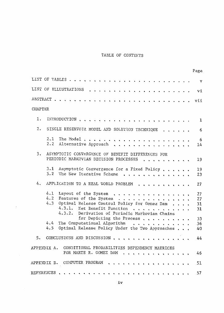
TABLE OF CONTENTS

Page

LIST OF TABLES

LIST OF ILLUSTRATIONS vi

ABSTRACT vii

CHAPTER

1. INTRODUCTION 1

2. SINGLE RESERVOIR MODEL AND SOLUTION TECHNIQUE 6

2,1 The Model 62.2 Alternative Approach 14

3. ASYMPTOTIC CONVERGENCE OF BENEFIT DIFFERENCES FORPERIODIC MARKOVIAN DECISION PROCESSES „ ...

3.1 Asymptotic Convergence for a Fixed Policy 3.2 The New Iterative Scheme

19

1923

4. APPLICATION TO A REAL WORLD PROBLEM 27

4.1 Layout of the System 274.2 Features of the System . . . 274.3 Optimal Release Control Policy for Gomez Dam . 31

4.3.1. Net Benefit Function 314.3.2. Derivation of Periodic Markovian Chains

for Depicting the Process 334.4 The Computational Algorithm 364.5 Optimal Release Policy Under the Two Approaches . , 40

5. CONCLUSIONS AND DISCUSSION 44

APPENDIX A. CONDITIONAL PROBABILITIES DEPENDENCY MATRICESFOR MARTE R. GOMEZ DAM 46

APPENDIX B. COMPUTER PROGRAM 51

REFERENCES 57

iv

LIST OF TABLES

Table Page

4.1 Statistical Parameters of Inflow for each Monthat Marte R. Gomez Reservoir 29

4.2 Monthly Evaporation from Gomez Reservoir 30

4.3 Optimal Release Policy for September 41

A.1 Conditional Probabilities Dependency Matricesfor each Month at Marte R. Gomez Dam 47

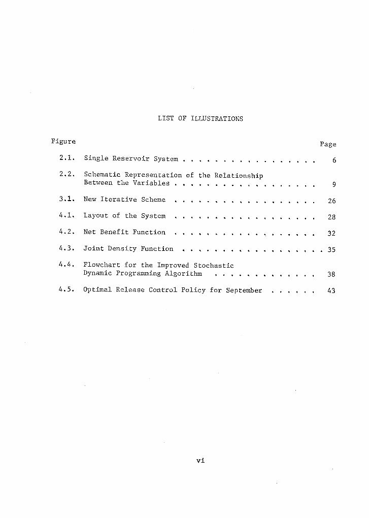
LIST OF ILLUSTRATIONS

Figure Page

2.1. Single Reservoir System 6

2.2. Schematic Representation of the RelationshipBetween the Variables 9

3.1. New Iterative Scheme 26

4.1. Layout of the System 28

4.2. Net Benefit Function 32

4.3. Joint Density Function 35

4.4. Flowchart for the Improved StochasticDynamic Programming Algorithm 38

4.5. Optimal Release Control Policy for September 43

vi

ABSTRACT

Stochastic dynamic programming has been widely used to solve

for optimal operating rules for a single reservoir system. In this

thesis a new iterative scheme is given which results to be more ef-

ficient in terms of computational effort than the conventional

stochastic dynamic approach. The scheme is a hybrid one composed of

the conventional procedure alternating with iterations over a fixed

policy in order to increase the chance of finding the optimal policy

more rapidly. Likewise this thesis introduces a refined technique to

derive transition probability matrices and the use of bounded vari-

ables in the recursive equation to provide an easier way to verify

the convergence of the cyclic gain of the system. A computer program

is developed to implement the new iterative scheme and then it is ap-

plied to a real world problem in order to derive quantitative compari-

sons. A real savings of twenty-five percent of the computational

time required with the conventional procedure is obtained with the

new iterative scheme.

vii

CHAPTER 1

INTRODUCTION

There is a substantial body of literature on the solution of

the optimal operating rule problem for a single stochastic reservoir.

Linear programming models, dynamic programming models and policy

iteration models have all been used, as reviewed by Loucks and Falkson

(1970).

Most of the work on the stochastic linear programming approach

to this problem has been done by Loucks (1969). This approach is in-

genious but computationally difficult. An unreported experiment by

Theodore G. Roefs (1974) was conducted in 1968. A twelve season

problem was solved using both the linear programming approach and the

stochastic dynamic approach. The linear programming approach required

more than an order of magnitude more computer time and the dynamic

programming approach. Hassitt (1968) shows the relationship between

the models.

Most of the work on the policy iteration approach to this

problem has been done by Howard (1960), The policy iteration method

has some of the features of both linear and dynamic programming ap-

proaches. Like all linear programming problems it is necessary to

solve sets of linear simultaneous equations, which even for small

problems can become quite large. As in dynamic programming problems,

the policy iteration method develops a recursive relationship which

1

2

is divided into two steps in an effort to examine only the steady sta-2

values, i.e., those that apply when a large number of transitions re-

main before the economical and hydrological conditions change.

The difficulties associated with Howard's (1960) method when

the number of states is large have been pointed out by White (1963),

Odoni (1969) and MacQueen (1966). In fact, an experiment reported by

Odoni (1969), for ten state and twenty-five state problems with three

alternatives per state, the stochastic dynamic approach reduced com-

putation time to one half and one fifth respectively, of the time re-

quired for policy iteration solution.

There is an additional drawback for linear programming models

and policy iteration models. There is no doubt that the number of

simultaneous linear equations that can be accurately solved on cur-

rent day computers is less than the number that may be requested for

a particular reservoir operation system. In the process of solving

large linear programming problems, computer roundoff and truncation

errors may result in an initially feasible solution becoming infeas-

ible. This obviously constraints the size of the problem that can be

examined using techniques such as in linear programming or those de-

veloped by Howard (1960). If the dynamic programming approach is

used, the solution of simultaneous equations is not required,

White (1963) first modified the method of successive approxi-

mations (dynamic programming) developed by Hellman (1957), for solving

Markov decision problems to focus attention on the convergence of costs

relative to the cost of a base state (cost differences ), rather than

on convergence of the total cost function.

For the undiscounted case he proved that the modified cost

function converged at least geometrically, irrespective of the se-

quence of policy chosen. Schweitzer (1965) proved convergence for

the more general single•chain aperiodic case. MacQueen (1966) and

Odoni (1969) have extended White's (1963) results to provide com-

putable upper and lower bounds on the gain of the process at each

iteration.

Su and Deininger (1972) likewise extended Odoni's (1969) re-

sults to the case where the Markovian decision process is periodic.

The method used for solving the periodic Markovian decision problem

consists in a simple backward recursive optimization routine. Owing

to the periodicity of the Markovian process, the maximal expected

payoff per cycle, instead of the maximal expected payoff per transi-

tion, is recursively computed until this value from every state suf-

ficiently converges to a constant. The converged constant would be

the desired approximated maximal expected average payoff per cycle,

and the policy used in the last iteration (in the cycle) is the de-

sired optimal policy.

Vleugels (1972) has demonstrated that Su and Deininger's

(1972) model can be simplified in order to consider a Markov process

with monthly transitions instead of a model with yearly transitions.

By decomposing the problem into one of monthly transitions, the

3

4

optimization problem decreases in size substantially. Additionally,

Vleugels (1972) demonstrated rather elegantly the properties of con-

vergence of this model through the use of contraction mapping tech-

niques. Vleugels' (1972) model is basically what the author considers

as the stochastic dynamic programming approach (SDP).

The technique used to solve the model consists of a simple

backward recursive optimization algorithm linked with a stopping pro-

cedure. The stopping procedure most generally employed consists of

the termination of the algorithmwhen the policy repeats itself in two

successive cycles. However, in theory a policy that repeats itself

need not be optimal, not even if there is only one optimal policy. In

this case, convergence of the modified cost function guarantees opti-

mality of a repeating policy. Obviously, after that point, one is in-

deed iterating a fixed policy. It is necessary for the modified cost

function to converge to guarantee that this policy will, in fact, be

optimal.

Morton (1971) has studied the asymptotic convergence rate of

cost differences for the case of a fixed policy. He demonstrated

that the modified cost function converges geometrically to the yearly

gain of the process. Additionally, he extracted an interesting im-

plication that can be summarized as follows: if the problem is "well

behaved" in the sense that policies with gains close to that of the

optimal policy also have transition matrices very similar to that of

the optimal policy, then one would expect convergence characteristics

"close to" that for a fixed policy.

5

This implication, together with the fact that the optimal

policy (if there is one) is often reached very early, lead us to the

conclusion that a hybrid iterative scheme composed of the conventional

procedure alternating with iterations over a fixed policy might be

more efficient in terms of computational effort than the conventional

procedure. The object of this thesis is to establish the theoretical

basis for the new algorithm and to establish its advantages.

To pursue such goals this thesis is organized in the following

manner. Chapter 2 introduces the Markovian model of the single

reservoir system and its corresponding conventional dynamic program-

ming formulation. Chapter 3 extends the results of asymptotic con-

vergence over a fixed policy, as derived by Morton (1971), to the

more general case where the Markovian decision process is periodic.

The new iterative scheme is presented at the end of this chapter and

its principal characteristics are exposed. Chapter 4 presents a case

study where the new technique is applied and compared with the tra-

ditional approach. First, a physical characterization of the system

is given. The refined technique to compute state transition proba-

bilities is then introduced. Thirdly, quantitative comparisons are

made between both approaches and computational implications are drawn.

Finally, Chapter 5 presents some general conclusions and discussion

of the study.

CHAPTER 2

SINGLE RESERVOIR MODEL AND SOLUTION TECHNIQUE

The water reservoir system under consideration will be

modelled as a Markovian Decision Process, The solution technique

used to solve the model will be stochastic dynamic programming and

it is presented in this chapter,

2.1 The Model

Consider Figure 2.1 which is a diagrammatic representation of

the single reservoir system, where St'

it

and rt are the initial

storage volume, streamf low input and release, respectively, for some

month t.

rt

Figure 2.1. Single Reservoir System.

6

7

Two major assumptions with respect to the stochastic process

of inflow should be established before the system can be modelled as

a Markovian decision process.

Assumption 1: The inflows in every time interval (a month)

to the reservoir are statistically dependent on the inflow of the

preceding interval.

Assumption 2: The stochastic process of these inflows is

periodic with period T; T time intervals define a cycle (T = 12

in this case).

Given Assumptions 1 and 2 it is possible to represent the

stream flow input to the reservoir as a Markov chain which is peri-

odic with a period of twelve months. The stochastic process is de-

fined by a set of probabilities of the form P(itiit-1)'

Since these

are conditional probabilities

it

p(it/i

t-1) = 1, for all

0 < p(i t/i) 1, for all it, it-1

The following notation will be used in this thesis:

- number of months in a year, T = 12;

- number of time interval in the cycle, t = 1, 2, ..„ T;

- time horizon in years;

- number of years remaining until the termination of the process,

n = 0, 1, 2, ..., m;

St

- storage volume of reservoir at the start of month t;

St+1

- storage volume of reservoir at the start of month t + 1;

it

- streamflow input to reservoir during month t;

t+1 - streamflow input to reservoir during month t + 1;

rt

- release from the reservoir during month t.

Figure 2.2 exhibits a schematic representation of the rela-

tionship between the variables previously defined.

The governing equation of the single reservoir system is:

St+1

= St + i

t - r

(2,1)

which states that the storage volume at the beginning of month t + 1

is equal to the sum of the initial storage volume and streamflow input

of month t minus the release made during month t, where the re-

lease is made according to the following decision process. The de-

cision process is to decide upon the release rt to be made after

observing the state (St, it-1) of the system, i.e., the decision is

made after observing the storage at the beginning of month t and

previous inflow in month t 1.

m - 1 0

1 IT 1121 N I IT 12j I I I I = t

9

Real time progressin this direction

(b)

it

rt

Oct. 1stSept. 1st

St s t+1

Figure 2.2. Schematic Representation of theRelationship Between the Variables.

• (a) Schematic Representation of• the Time Variable.

(b) Time Relationship BetweenModel Variables.

1 0

The decision variable rt is constrained by LC < r < UCt — r — t

for each t, where LCt and UCt are the prescribed minimum and

maximum permissible drafts. Physically these limits could correspond

with obligatory release and channel capacity, respectively, Addition-

ally the water storage levels of the reservoir are bounded above by

the physical size limitation of the reservoir; below by the minimum

storage level at which the water can be extracted from the reservoir.

Any r t , such that LC t < r t < UC t , will be a feasible de-

cision, An operating policy is a set of feasible decisions that indi-

cates what action is to be taken after observing the state (S1

)

of the system.

For mathematical manipulation, let all variables be dis-

cretized taking some finite number of discrete values. Now, assume

that it is possible to derive monthly transition rewards of the form

Vt(r

t) - Immediate reward when the system makes a

monthly transition from month t to month

t + 1, when the release is r.

Let us assume also, that the immediate reward is independent

of the year of the process, that is

VT+t

(r t) = V(r) for all t. (2.2)

11

It is also possible to derive monthly transition probabilitie-

of the form

P[(S1

).r Probability to transitioning to state

+ t ' t

(St+1,it) given the system is in

state (St'it-1)'

where the release

was r in month t.

Where by Assumptions 1 and 2 and the forcing equation (2.1)

it is obvious that

P[(St-1 )(St+1

);r ]t t t

t-1) if S

t+1 = S

t +i

t - r

t

(2.3)

otherwise

which simply says that if the policy specifies a particular final

reservoir volume St+1

in period t + 1 for an initial storage

volume St and inflow it

in period t then the state transition

probability equals the inflow transition probability, otherwise the

probability of that particular state is zero.

Now consider the system as a stochastic process observed at

discrete points t to be in one of a finite number of states

(S' it-1')* (Stt-1) is a periodic Markovian process with period T

t

and has transition probabilities given by (2.3). The reservoir

12

system can be thought of as making transitions from one state

(Sc i t_ i) to another state (St+1t

) in successive periods. If

there are T periods in a year, then t proceeds from 1, 2, 3,

T - 1, T, 1, 2, ..., to some distant time horizon m years or

mT periods in the future.

GivenAssumptions 1 and 2 and equations (2.1) and (2.3), it is

now possible to derive the mathematical model for the system. Con-

sider that the system is currently at the beginning of a time interval

that is (n + 1)T - t + 1 intervals from termination. At this time

the system is observed to be in state (St 'it-1)

in period t. If a

decision r made from a finite set of feasible decisions, then

an immediate reward V(r) is obtained, and the system moves to a

state (St+1'it)

at the end of this interval following the proba-

bility function P (it I it-1) Note that the reward in each period

is independent of the inflow it .

Let f(n+1)T-t+1(St'it-1)

be the maximal total expected

undiscounted reward from the next (n + 1)T - t + 1 intervals. Thus

with (n + 1)T - t + 1 = 1 period to go, the total expected reward

is

f1(Stt-1

) = Vt (rt), for all S t , j_ '

rt = f(S+1' i

' S )"(2 4)t t t

With (n + 1)T - t + 1 = 2 periods to go, the total expected

reward is

13

f2(St't-1) = V(r) p(i t/i

t-1)f

1(St+1't

)'

for all St

,t-1'

rt

= f(St,s

t+1'it)

where each fi (S ti_v i t) was determined by equation (2.4). In general

the recursive relationship for determining the total expected reward

with (n + 1)T - t + 1 stages to go, given a particular operating

policy (a fixed policy) rt = f(S

t'St+1

), is

df(n+1)T-t+1(3t'it-1 = Vt(r+ ' •)

It

t'/i t-1')f (n+1)T-t (S

t+1'it

) •

An optimal policy is defined as one that maximizes the expected

total reward, that is

(S i ) = Max[V (r ) + y p(i /i )ff(n+1)T-t+1 t' t-1 t t . t t-1 (n+1)T-t

(St+1't

)]

it

for all S t it-1' "

(2.5)

Starting at some time in the future and using the connection

between the inflows in one time period and the adjacent time period

it is possible to calculate values of rt for each time period as a

function of the state variable (St't-1). These r

tts then form

an optimal policy of the operation of the reservoir. The important

point to note is that under conditions of ergodicity of the process

this policy is said to converge when the values of rt that are used

14

to evaluate the function f (n + 1)T - t + l(St'it-1) repeat for all

values of t when the number of transitions becomes larger.

Howard (1960) proved that an optimal policy will converge if

the system is ergodic. This term implies that the final state of the

system is independent of the starting state. In other words this is

equivalent to stating that no matter what the state of the reservoir

at the start of the computations the steady state of the system will

be independent of the starting state.

2.2 Alternative Approach

Equation (2.5) is the application of the "Principle of

Optimality" of dynamic programming to the Markovian decision process

as stated by Bellman (1957). It can be solved straightforward using

a backward optimization routine. However, an alternate procedure is

still feasible if we now consider the Markovian process as an aperiodic

one. That is, if we can derive an equivalent equation to that of

(2.5) but now transforming the periodic process to one that is

aperiodic, such alternate approach can be accomplished.

Now, let us introduce an operator At

defined for any func-

tion h by

Ath(S

t+1t) = Max[V (r ) + p(i /i1 )h(St+1 )] for allt t . t t- trtt

S t+1' it t

15

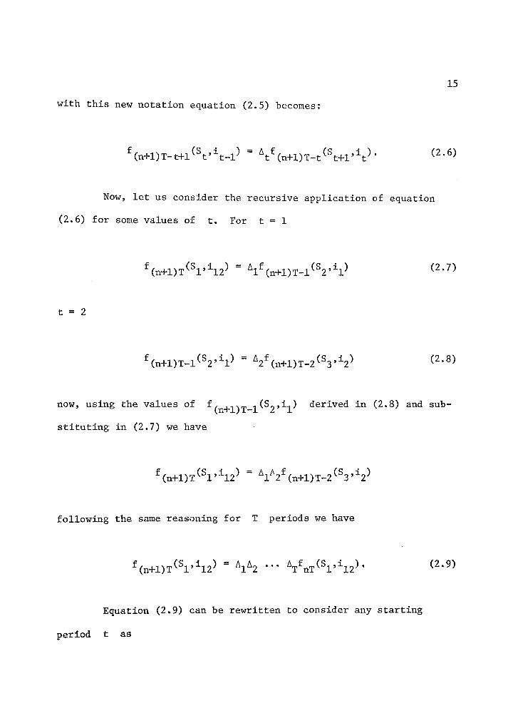
with this new notation equation (2.5) becomes;

f(n+1)T-t+1 (S

t' it-1) = A tf (n+1)T-t (S

t+1t). (2.6)

Now, let us consider the recursive application of equation

(2.6) for some values of t. For t = 1

f(n+1)T

(Si12) = A1f(n+1)T-1(821)

(2.7)

t= 2

(n+1)T-1 (S 2' 1l ) = A2 f (n+1)T-2 (S3' i2 )(2.8)

now, using the values of f(n1)T-1(S2'i1)

derived in (2.8) and sub-

stituting in (2.7) we have

f (n+1)T (S112) = A1A 2f (n+1)T-2 (S

3' )

following the same reasoning for T periods we have

f (n+1)T (Sl' 1l2 ) = hA2 ". &I•fnT (S l' il2).

Equation (2.9) can be rewritten to consider any starting

period t as

(2.9)

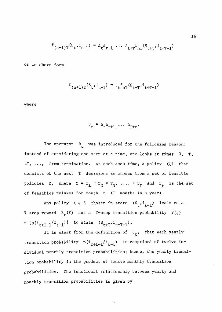
16

f(n+1)T (Sc it_i) = 't

At+1 ". A t+T fnT (S t+T' it+T-1 )

or in short form

f(n+1)T (S t' it-1 ) = e tfnT (S t+T' it+T-1 )

where

Ot =Lt ...tt+1

AT+t

.

The operator et

was introduced for the following reason;

instead of considering one step at a time, one looks at times 0, T,

2T, from termination. At each such time, a policy (C) that

consists of the next T decisions is chosen from a set of feasible

policies Z, where Z = rl x r2 x r 3 , .,„ x rT and r

t is the set

of feasibles relases for month t (T months in a year),

Any policy CCZ chosen in state (S' it-1 ) leads to at .

T-step reward Rt (C) and a T-step transition probability 17(c)

= [P(it+T-llit-1)] to state it+T-1).

It is clear from the definition of et' that each yearly

transition probability p(iT+t-1/i

t-1) is comprised of twelve in-

dividual monthly transition probabilities; hence, the yearly transi-

tion probability is the product of twelve monthly transition

probabilities. The functional relationship between yearly and

monthly transition probabilities is given by

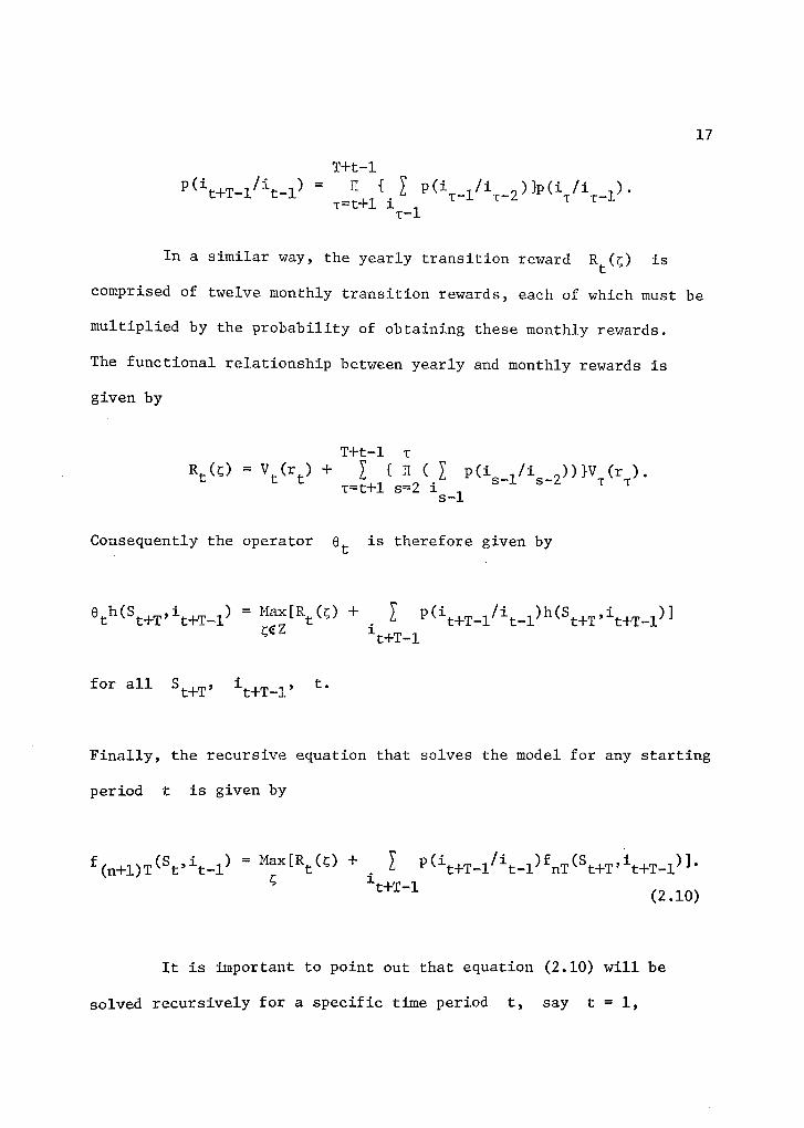
17

T+t-1

11t = TI { X p(i1 /1T-2 )}13(i /I ,

I).T- T T-T=t+1

T-1

In a similar way, the yearly transition reward R(r) is

comprised of twelve monthly transition rewards, each of which must be

multiplied by the probability of obtaining these monthly rewards.

The functional relationship between yearly and monthly rewards is

given by

T+t-1 TRt = V(r) + y {11(X P(i ,/i ,))1V (r ).S-1 S -G T TT=t+1 s=2

s-1

Consequently the operator e t is therefore given by

e th(St+Tt+T-1) = Max[R.t + X p(it+T-1/i

t-1)h(S

t+T'it+T-1)1i

t+T-1

tfor all St+Tt+T-1,•

Finally, the recursive equation that solves the model for any starting

period t is given by

f(n+1)T

(Stt-1

) = Max[Rt

+ X p(it+T-1

/it-1

)fnT

(St+T't+T-1

)]

t+T-1 (2.10)

It is important to point out that equation (2.10) will be

solved recursively for a specific time period t, say t = 1,

18

since all the remaining periods are taken implicitly into account by

the equation.

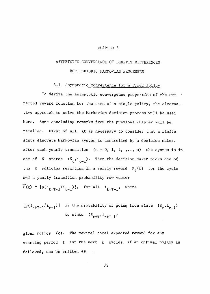
CHAPTER 3

ASYMPTOTIC CONVERGENCE OF BENEFIT DIFFERENCES

FOR PERIODIC MARKOVIAN PROCESSES

3.1 Asymptotic Convergence for a Fixed Policy

To derive the asymptotic convergence properties of the ex-

pected reward function for the case of a single policy, the alterna-

tive approach to solve the Markovian decision process will be used

here. Some concluding remarks from the previous chapter will be

recalled. First of all, it is necessary to consider that a finite

state discrete Markovian system is controlled by a decision maker.

After each yearly transition (n = 0, 1, 2, .„, m) the system is in

one of N states (Stt-1).

Then the decision maker picks one of

the Z policies resulting in a yearly reward R(t) for the cycle

and a yearly transition probability row vector

= [p(it+T-1

/it-1

)1, for all 1t+T-1'

where

[P(it+T-1/it-1)] is the probability of going from state (St

'it-1)

to state (St+T't+T-1

)

given policy (O. The maximal total expected reward for any

starting period t for the next n cycles, if an optimal policy is

followed, can be written as

19

20

f(n+1)T (S

t'it-1

)

(3.1)

= Max[Rt (c) +

X p(i t+T-1 /it-1 )fnT (S

t+T' it+T-1 )].t+T -1

Since the term / P(it+T-1/it-1 )fnT (St+T't+T-1) can be written

matrix gt (01, times a column vector T

equation (3.1) can be

written as

f (n+1)T (St't-1

) = Max[Rt

+ (c) ]. (3.2)

Considering now the vector f(n+1)T that includes all the

elements f (n+1)T (Sc it_1), the following vector equation can be

written:

= Maxfkt P (C)1Tia l,T(n+1)T

—where R

t() is the yearly reward vector and {P(c)} is the yearly

transition matrix.

Let us consider the case of a fixed policy for which in the

stationary condition a yearly transition probability matrix {P} and

a yearly transition reward vector R have been permanently achieved.

This statement is translated mathematically to the following

equation:

it+T-1

as the product of a row vector belonging to the transition

21

1-(n+1)T = {P}1-11T . (3.3'

Writing out values of (3.3) for some particular values of n

we have for n = 1;

T-T = "K: {p}1-o (3.4)

for n = 2;

T2T = R + {F}TT. (3.5)

Substituting the value of 1-T, obtained in (3,4) into (3.5)

yields,

T-2T

= {P}[-i+ {P}T

Simplifying, we have

T-2T = -R- + {P}T¢- + {P} 2 fo

Following a similar reasoning an expression for 13T is

obtained as follows

= + {P}R + {P} 2—R + {p} f 0

In general, for n = n we have,

22

(n+1)T = {PlaR + {P}n+1

Ta=0

(3.6)

Assuming that {P} has N distinct real eigenvalues 1, yi ,

Y 2' • 1N-1' where 1 L I yit 1y21 L • • • IY1 _11, and using

results obtained by Howard (1960, pp. 9-12), an expansion for {P} a

can be written as

N-1{P

}a = {S} +

j=1

where {S} has identical rows which represent the stationary proba-

bilitiesand{T.lare the transient matrices,

New terms are defined in the following way;

= {SiT = k0 0

and {Tj}T = r

j where e = is a unit column vector.

—Thus, k is the generalized yearly gain, while q ., and r

J

are transient error vectors.

Then equation (3.6) is rewritten as:

n N-1 N-1

17(n+1)T = ((ke + X Ya.7(i.)) -L

a0 j=1(3,7)'0'

= j j

= 3 3 j1

In a similar manner it is possible to derive an expression

for TnT as follows:

23

n-1 N-1InT :0k

(k-e + y .) + k0 +

N-1 yr7.

j=1 J J = j=1

—Defining a new vector x

n as:

].-Tc = f(n+1)T fnT •

From the above it follows directly that

; n = ± (Y1 - 1)171 ) g (Yn2 Yn3(3.8)

As n + it is reasonable, in equation (3,8), to neglect

the terms compounded by the eigenvalues of minor dominance and ex-

clusively consider the term with yl .

—It is clear from equation (3.8) that the sequence {Xn

} will

converge geometrically to the limiting value 1Ce- (by definition the

cyclic gain of the process) as n + co.

3.2 The New Iterative Scheme

Howard (1960, pp. 40-41) demonstrated that using values for the

functional f (n+1)T-t+1 (5tt-1) obtained by searching over the steady

state values for a particular given policy, the new policy derived

from this new set is better than the older ones. Such improved

values are obtained in Howard's (1960) policy iteration method through

the solution of a set of N simultaneous linear equations, where N

24

is the number of discretized states. It is clear that such pro-

cedure is very limitative when the number of states is very large,

which is the usual case in operation reservoir problems, However,

in light of the results of Section 3.1, it is absolutely clear that

it is no longer necessary to do the improved values step by solving

a set of simultaneous linear equations. Simply repeatedly using the

successive approximation machinery with the policy kept fixed will

produce both the yearly gain of the process and the modified benefit

function with geometric convergence. It is relevant to note that

this machinery is used by the conventional stochastic dynamic approach

in any event, so that the programming needed for the improvement pro-

cedure is actually a subset of that for the conventional approach.

In fact, these steady state values can be obtained through a

routine that is quite similar to that developed for the full maxi-

mizing step (equation 2.5) of the conventional approach. However,

instead of lookng through all feasible alternatives (releases from

the reservoir) for each state, one computes only the cyclic gain of

the system and the improved values for the releases fixed. The

asymptotic convergence of the cyclic gain of the process guarantees

that the improved values for the functional will, in fact, be drawn

from the steady state condition.

Moreover, from the author's experience, the number of itera-

tions required to obtain the desired convergence with a maximum

error of one percent (1%) is at most two in the early stages when

25

the current policy is far from the optimal, and one iteration in the

middle and final stages when the current policy is very close to the

optimal.

With these ideas in mind, a combined iterative routine can

be sketched. Figure 3.1 shows the proposed algorithm. Here, instead

of using the linear diverging variable f(n+1)T-t+1(St'it-1) which

is inconvenient from a practical point of view, the bounded variable

f' (S I)(n+1)T-t+1 (St' it-1 ) = f (n+1)T-t+1 (S t' it-1 ) f (n+1)T-t+1 t' t-1

(s l ,i l )is preferred, where refers to the value off(n+1)T-t+1 t t-1

the functional for a base state (S'' il

1 )t t-

26

Step 1 - Starting Procedure:Set f' (St+1, 1 t

) equal zero for

that T + 1 = 1.(n+1)T-t

n = 0, t = T and considering

Setn0=

Step 2 - Full Optimization Routine: Solve for t = 12, 11, 10, ...,

p(i /i )f . (S ,i )),t t-1 n+1)T-t t+1 t -

)

- f (n+1)T (Sl' il2 ) '

i' ) is a base state.l' 1

n+1)T-t+1(S

t'it-1

) = Max(V (r ) +t t .r i

tt

for all (St,i

t-1

Store r* which is optimal.tCompute Bounded Variables:

f (n+1)T ' il2 ) = f (n+1)T (5 l' 1l2 )

for all (S1 ,i ), where (S'

Step 3 - Stopping Procedure: If

A < Elf (st it )1

— (n+1)T l' 12 '

number.

(If (S',i' ) - f (S' i'(n+1)T 1 12 nT l' 12

where C is a small positive

If "YES" Stop.

NO

Step 4 - Improved Values Routine: Compute for t = 12, 11, 10„..,

/i )f' (S ,i ),t-1 (n+1)T-t t+1 t

i12

) - f(n+1)T l' 12 '

n + 1. Go to Step 2.

f e (S ,i ) = V (r ) X p(ik,n+1)T-t+1 t t-1 t t ti t

using the rt of Step 2.

Update Bounded Variables:

f(n+1)T(S1,i12) = f (n+1)T (5 i

for all l'12•Set n =

Figure 3.1. New Iterative Scheme

CHAPTER 4

APPLICATION TO A REAL WORLD PROBLEM

The real system that was chosen with the purpose of testing

the new iteration scheme is Marte R. Gomez Reservoir on the San Juan

River in Northeastern Mexico.

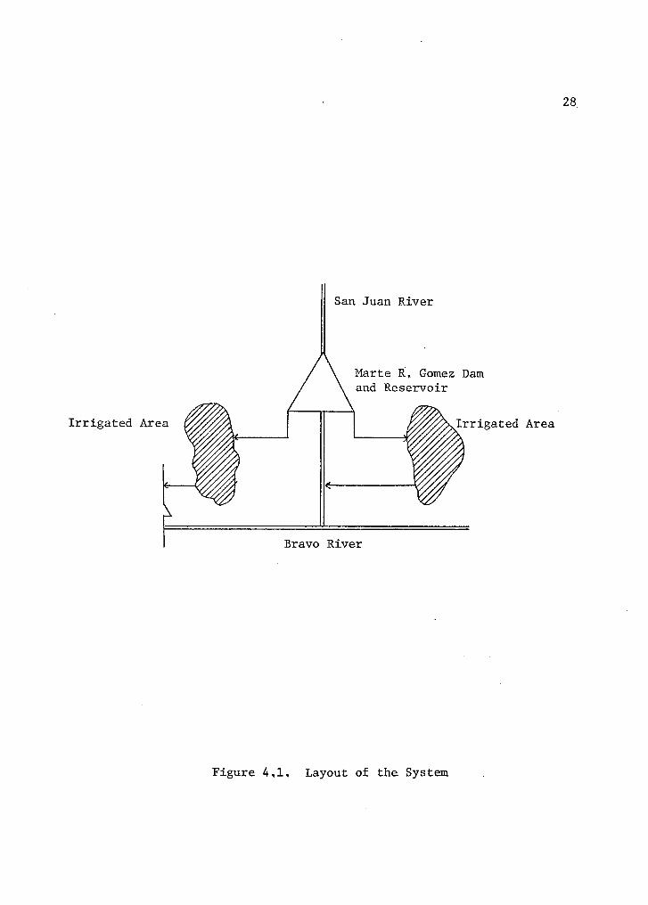
4.1 Layout of the System

The system is composed of five elements, namely, the river that

provides the inflow, the reservoir that stores the water, and three

main channels that serve the water requirements downstream. A sche-

matic layout of this system is shown in Figure 4.1. The system is

part of a more complex one. The integrated by the set of reservoirs,

diverging dams, main channels, flood ways, power plants, etc„ that

conforms the total Bajo Rio Bravo and Bajo Rio San Juan system.

4.2 Features of the System

The system was constructed in 1943 for irrigation purposes

exclusively. The streamf low data correspond to the historical record

that was registered in the period 1902-1941 at Santa Rosalia Station,

that was located upstream of the dam. In the period 1944-1964 the

streamf low data were deduced from the monthly functioning of the dam.

The historical record consists of fifty-three years of mean monthly

flows, expressed in millions of cubic meters. The mean monthly flows,

27

Irrigated Area Irrigated Area

San Juan River

28

AMarte R. Gomez Damand Reservoir

Bravo River

Figure 4,1. Layout of the System

29

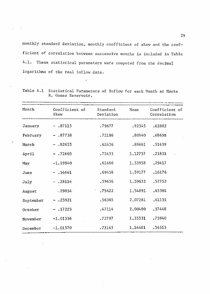
monthly standard deviation, monthly coefficient of skew and the coef-

ficient of correlation between successive months is included in Table

4.1. These statistical parameters were computed from the decimal

logarithms of the real inflow data.

Table 4.1 Statistical Parameters of Inflow for each Month at MarteR. Gomez Reservoir.

Month Coefficient of Standard Mean Coefficient ofSkew Deviation Correlation

January - .87115 .79677 .92345 .62882

February - .87738 _.72186 .80940 .68698

March - .82655 .62436 .88661 ,51639

April - .72603 .72433 1.12757 .21831

May -1.19940 ,61466 1,53958 .29417

June - .54641 .69438 1,59177 .16176

July - .28116 .59656 1.59633 ,52752

August .29834 ' ,75622 1,54891 .45301

September - .25921 ,56365 2,07281 ,61131

October - .17223 .47114 2,00480 .37448

November -1.01336 ,72797 1.35531 .75940

December -1.01570 .73163 1,16481 .54513

30

Marte R. Gomez dam is an earth dam of forty-nine meters

height. The reservoir has a maximum capacity of 1100 million cubic

meters and a dead storage volume of 100 X 106m3

approximately.

Evaporation losses are expressed as the average monthly voluem lost

and will be considered a constant for a particular month, indepen-

dently of the year. The monthly evaporation volume losses are in-

cluded in Table 4.2.

Table 4.2 Monthly Evaporation from Gomez Reservoir

Month

Volume (106m3)

January 9.2

February 10.7

March 15.6

April 18,6

May 20,7

June 22,5

July 35,9

August 22,2

September 18,3

October 16,3

November 11,8

December 9,4

31

The relase schedule of Gomez Dam is limited by a maximum

amount, given by the total capacity of the conduits, totaling

200 X 106m3

per month.

No flood control is provided in Gomez Reservoir, since the

spillway is of the free type, i.e., there are no control facilities.

Minimum requirements for monthly releases are implicit in the benefit

function.

4.3 Optimal Control Policy for Gomez Dam

4.3.1. Net Benefit Function

For the purpose of this study the unit price of water will be

considered constant. A monthly target output of 100 x 106m3 is

included in the benefit function. Penalty costs are imposed over

monthly releases below the monthly target output,

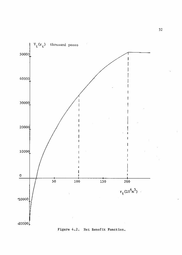
A smooth variation of the net benefit function is obtained by

fitting a parabolic equation to three match points given by the value

of the function when the release is zero, one hundred and two hundred

million cubic meters respectively. Equation (4.1) and Figure 4,2

express these concepts analytically and shematically,

Vtt

) = 52500 - 1,75(rt

200) 2 (4,1)

The returns in different time periods will not be discounted,

This case is not covered in this study. However, no substantial

50 100 150 200

rt (10 6m3 )

32

Figure 4.2, Net Benefit Function.

33

changes have to be made in the mathematical formulation of the process

to include it.

4.3.2. Derivation of Periodic Markovian Chains forDepicting the Process

The state transition probabilities for the case study can be

derived from the monthly inflow probability distributions (conditional

and unconditional). The state transition probabilities can then be

computed from these probabilities and the governing equation (equa-

tion 2.1). Computationally, only twelve sets of monthly inflow

probability distributions must be stored in the computer, and every

state transition probability is computed, when it is being used, ac-

cording to the equations stated in (2.1) and (2.3).

The twelve sets of probabilities for the monthly inflows were

derived using a refined technique developed by Clainos (1972) based

on a stochastic streamflow synthesis technique.

At each time t the continuous value of each monthly inflow

it

is discretized into a finite number of equal intervals. Each

interval is, then represented by the value at its midpoint. This

discretization scheme provides a convenient way of indexing the

various values of it and it is easier to program for the computer.

Using the definition of conditional probability, the con-

ditional probability P(A/B) is desired where P(A/B) = P(A,B)/P(B).

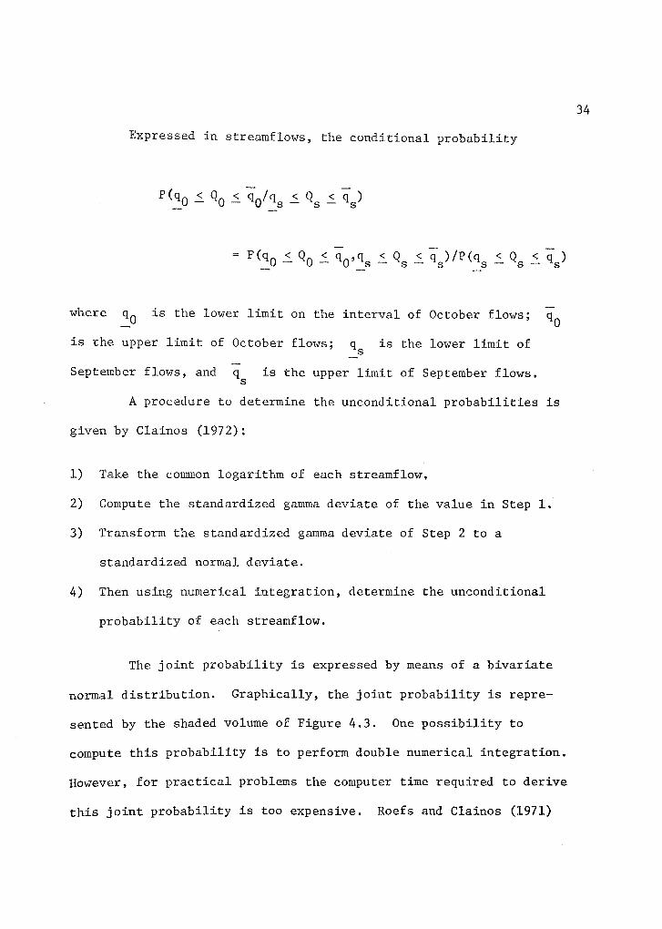
Expressed in streamf lows, the conditional probability

P (q0 QO (10 / cis < Q s qs )

= P ( clo Q0 < )/13(c1 )— s0 s— s

where q, is the lower limit on the interval of October flows; q0

is the upper limit of October flows; s is the lower limit of

—September flows, and qs is the upper limit of September flows,

A procedure to determine the unconditional probabilities is

given by Clainos (1972);

1) Take the common logarithm of each streamflow,

2) Compute the standardized gamma deviate of the value in Step 1.

3) Transform the standardized gamma deviate of Step 2 to a

standardized normal deviate.

4) Then using numerical integration, determine the unconditional

probability of each streamf low.

The joint probability is expressed by means of a bivariate

normal distribution. Graphically, the joint probability is repre-

sented by the shaded volume of Figure 4.3. One possibility to

compute this probability is to perform double numerical integration.

However, for practical problems the computer time required to derive

this joint probability is too expensive. Roefs and Clainos (1971)

34

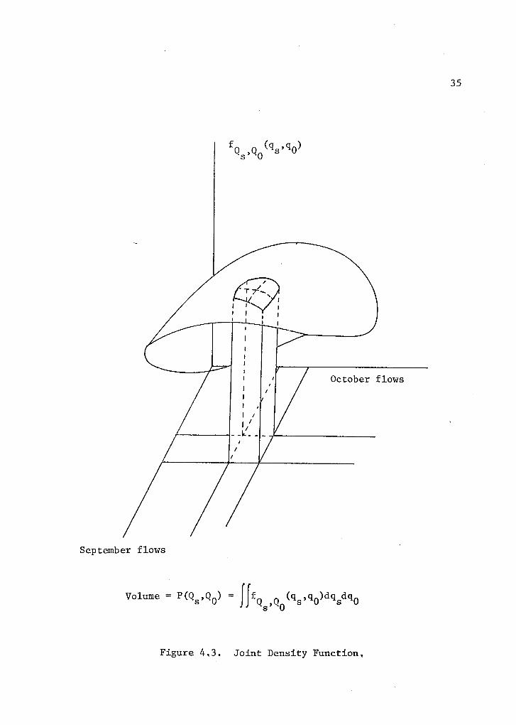
September flows

35

Volume = P(Q s ,Q 0) = iffQs,Q0 (qs ,(10)dqsdq0

Figure 4 3 . Joint Density Function,

36

show that if the flow interval of the previous month was sufficiently

small, it could be represented by a single point. If this approxima-

tion is made, the computational effort is reduced substantially. A

computer program is provided by Clainos (1972) to derive conditional

probabilities matrices.

Problems arising from high skewed streamflows (g > 2) was

studied by Clainos, Roefs, and Duckstein (1973). These problems arise

because the Wilson-Hilferty transform is used to transform a Pearson

type III deviate to a normal deviate. Clainos et al. (1973) provide a

new transform based on Harter's (1969) work. Basically, he computed

the percentage points of the chisquare distribution, which he then

modified to percentage points of the Pearson III distribution, Clainos

et al. (1973) show that this new transform works very well for coef-

ficient of skew as great as three inclusive.

However, in this study the use of the new transform was not

necessary since the coefficient of skew for all months are less than

+ 1.5.

Appendix B shows the conditional probabilities dependency

matrices derived for each month.

4.4 The Computational Algorithm

A computer program was written in Fortran IV language and the

CDC 6400 computer was used to solve the recursive equation (2,5) of

Chapter 2 subject to all the constraints specified previously. For

the purposes of this study it was found that increments of 100

37

million cubic meters for the storage, and 10 million cubic meters

for the release are appropriate. However, the size increment for the

monthly inflow varies considerably depending upon the range of varia-

tion of these inflows for a particular month.

In view of the large range of variation of inflow for some

months, it was necessary to establish an upper limit of five incre-

ments to maintain the problem within the limits of computer time as-

signed to this study. Consequently, the increments for the state and

decision variables are not the same . This fact may lead to the re ,,

suit that during the iterations the next state is not necessarily one

of the original discretized states. Hence, some kind of interpolation

scheme must be used. The selected scheme for this study was linear

interpolation, mostly due to its simplicity, However, since the

benefit function is smooth and convex, a second order interpolation

polynomial would fit better to the benefit function than the linear

approach.

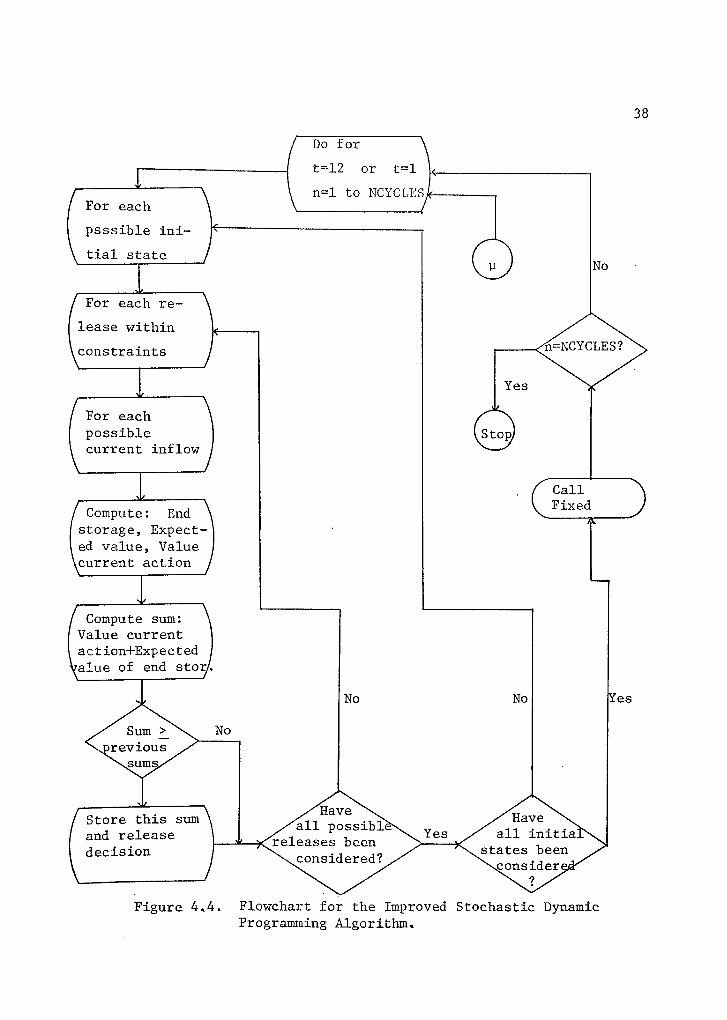
The computer program is composed of two parts. The first one

corresponds to the main program, where the data are read and the full

optimization step is located. The second part comprises the improved

relative values step and it is located in a subroutine which is

called every time a full maximizing step is executed. A flow chart

of the proposed algorithm is included in Figure 4.3. A listing of

the computer program is presented in Appendix A,

(CallFixed

Yes

Haveall possibl

releases beenconsidered?

/ Store this surn

\Land releasedecision

/ For each

psssible ini-

\ tial state

/ For each re- \

lease within

constraints

Yes

Compute: End \

(

storage, Expect-ed value, Valuecurrent action /

Compute sum: \

(

Value currentaction+Expectedalue of end stor/

Yes

No

Haveall initia

states beenconsider

38

Figure 4.4. Flowchart for the Improved Stochastic DynamicProgramming Algorithm.

39

/ For each

possible ini-

tial state

No

Compute:-end storage-expected v.of end storage-Value of cur-rent action

Compute sum:(value of currentaction -1- expected. of end storage/

Yes

No

Haveall possible

initial stateseen considere

Store this sum

40

4.5 0 timal Release Folic Under the Two A roaches

The conventional stochastic dynamic programming and the new

iterative scheme were tested in order to derive quantitative compari-

sons. As can be observed from the flowchart, the computational algo-

rithm for the conventional approach forms part of the composed

algorithm. Simply by avoiding the call to the subroutine FIXED the

algorithm for the conventional approach is obtained,

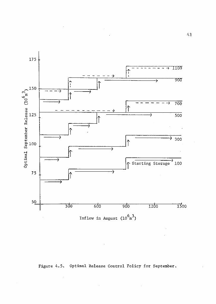
A sample of the optimum policy determination for September is

given in Figure 4.5 in graphical form and in Table 4.3 in tabular

form.

The expected annual returns for the conventional approach,

as determined by the gain of the system, was $363,594,000 with the

optimality criterion being equal to .001 (with a maximal pos-

sible error of 100x E percent). This condition was reached after

six full iterations and about fifty seconds of central processing

time were required. The optimal policy was obtained in the sixth

iteration.

The corresponding expected annual return for the new itera-

tive scheme, for the same level of accuracy, was $363,605,000. This

amount is practically identical as that obtained with the conven-

tional approach. Such condition was reached after four full itera-

tions and three fixed policy iterations, requiring thirty-eight

seconds of central processing time. The optimal policy was obtained

in the fourth full iteration, stopping the algorithm at this point

41

since the level of accuracy in the yearly gain of the system was

satisfied and the optimal policy reached.

Table 4.3 Optimal Release Policy for September

StartingStorage Inflow in August (10

6m3

)

106m3

150 450 750 1050 1350

100 70 80 80 90 90

200 80 90 100 100 100

300 90 100 100 110 110

400 100 110 110 110 120

500 110 120 130 130 130

600 120 130 130 130 130

700 130 130 130 140 140

800 130 140 140 140 140

900 140 150 160 160 160

1000 150 160 160 160 170

1100 150 160 160 170 170

It is important to notice that the decreasing computer time

would be proportionally greater if the number of discrete values of

the decision variable were increased. In this particular applica-

tion, only twenty discrete values of release were analyzed; in this

case it was necessary to expend approximately two seconds in the

42

execution of the fixed policy routine and eight seconds for the full

iterative step. However, in a more refined model where the number of

discrete values were three or four times the number of discrete

values used here, the fixed policy routine will remain costing ex-

clusively two seconds per iteration as compared with the full maxi-

mizing routine which will be increased at least three or four times

more.

For this particular application a saving of approximately

twenty-five percent of central processing time was obtained. How-

ever, based on the arguments of the above paragraph this saving might

jump to fifty percent,

175-

,,150

.00

1100

9-OTT

-5 700

43

I Starting Storage 100

75

50300 600 900 1200 1500

Inflow in August (106m3)

300

500

Figure 4.5. Optimal Release Control Policy for September.

CHAPTER 5

CONCLUSIONS AND DISCUSSION

The operating policies for a single stochastic reservoir

system are commonly optimized by conventional dynamic programming

with the use of high speed digital computers . However, this method

usually encounters two difficulties that constrain its general ap-

plication, namely, the untractable large computer memory requirement

and the excessive computer time requirement. The new iterative scheme

can, at least, ease the latter difficulty considerably. By examining

only the steady state values, those produced for a fixed policy after

the execution of each full maximizing step, an improvement in the

values of the functional used in the subsequent policy determinations

is obtained, increasing the chance of finding the optimal policy more

rapidly. Such improved values are obtained by simple repeated use of

the successive approximation machinery with the policy kept fixed.

The procedure will produce the improved values with geometric

convergence,

The time requirements with the proposed algorithm are reduced

by, at least, twenty-five percent (25%) of the time required with the

conventional approach. Moreover, if the number of discrete values

for the decision variable is increased, the computer time saved might

be raised proportionally up to fifty percent (50%). This saving

44

45

will have direct effect on the feasibility to deal with more sophis-

ticated systems that in the past have been untractable by the tra-

ditional technique.

At this point, it is important to mention that a general

drawback which is shared by all the stochastic dynamic programming

approaches to derive optimum operating policies is directly related to

the absence of control over their probability of failure s The tech-

nique is designed to maximize expected net benefits, and in doing so,

it may derive a policy that despite its economic advantages, will

allow the system to fail more frequently than the operating authority

is willing to accept. A further improvement of the algorithm pre-

sented is possible by introducing a technique developed by Askew

(1974) that permits the derivation of the optimal policy subject to

a constraint on the probability of failure. The technique consists

basically in the imposition of an extra penalty cost in the recursive

equation to be maximized.

APPENDIX A

CONDITIONAL PROBABILITIES DEPENDENCY MATRICES

FOR MARTE R. GOMEZ DAM

46

47

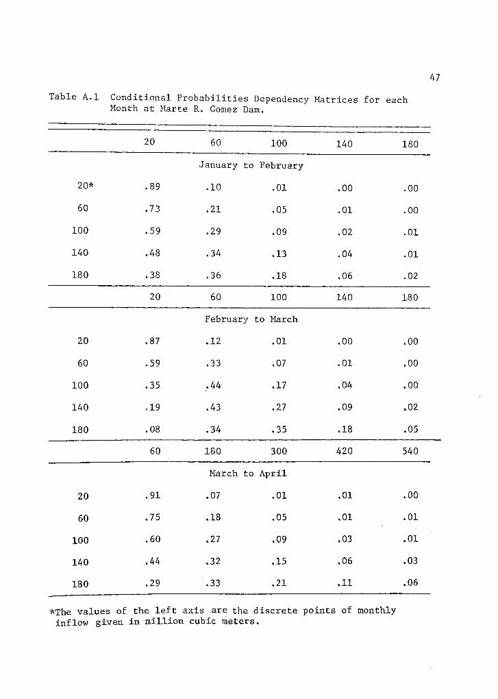
Table A.1 Conditional Probabilities Dependency Matrices for eachMonth at Marte R. Gomez Dam.

20 60 100 140 180

January to February

20* .89 .10 .01 .00 .00

60 .73 .21 .05 .01 .00

100 .59 .29 .09 .02 .01

140 .48 .34 .13 .04 .01

180 .38 .36 .18 ,06 .02

20 60 100 140 180

February to March

20 .87 .12 .01 .00 .00

60 .59 .33 .07 .01 .00

100 .35 .44 ,17 .04 .00

140 ,19 .43 .27 .09 .02

180 .08 .34 .35 .18 .05

60 180 300 420 540

March to April

20 .91 .07 .01 .01 .00

60 .75 .18 ,05 ,01 .01

100 .60 ,27 .09 .03 .01

140 ,44 .32 ,15 ,06 .03

180 .29 .33 .21 .11 .06

*The values of the left axis are the discrete points of monthlyinflow given in million cubic meters.

48,

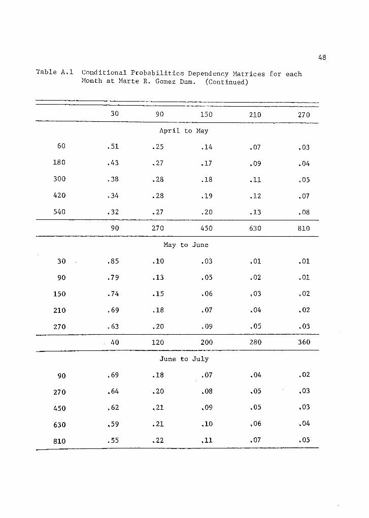
Table A.1 Conditional Probabilities Dependency Matrices for eachMonth at Marte R. Gomez Dam. (Continued)

30 90 150 210 270

April to May

60 .51 .25 .14 .07 .03

180 .43 .27 .17 .09 .04

300 .38 .28 .18 .11 .05

420 .34 .28 .19 .12 .07

540 .32 .27 .20 .13 .08

90 270 450 630 810

May to June

30 .85 .10 .03 .01 .01

90 .79 .13 ,05 .02 .01

150 .74 .15 .06 ,03 ,02

210 .69 .18 .07 .04 .02

270 .63 .20 .09 ,05 .03

40 120 200 280 360

June to July

90 .69 .18 .07 .04 .02

270 .64 .20 .08 ,05 .03

450 ,62 .21 .09 ,05 .03

630 ,59 .21 .10 ,06 .04

810 .55 .22 .11 .07 .05

Table A.1 Conditional Probabilities Dependency Matrices for eachMonth at Marte R. Gomez Dam. (Continued)

150 450 750 1050 1350

July to August

40 .93 .04 .02 .01 .00

120 .85 .09 ,03 .02 .01

200 .79 .12 .05 .02 .02

280 .74 .15 .06 .03 .02

360 .71 .15 .07 .04 .03

150 450 750 1050 1350

August to November

150 .66 .21 .08 .03 .02

450 .56 .25 .11 .05 .03

750 .51 .27 .12 .06 ,04

1050 .47 .28 .13 .07 .05

1350 .43 .29 .14 ,08 .06

150 450 750 1050 1350

September to October

150 .88 .10 .02 .00 .00

450 .68 .23 .06 ,02 .01

750 .56 .29 .10 .04 .01

1050 .47 .32 ,13 ,05 .03

1350 .40 .37 .15 .07 .03

49

50

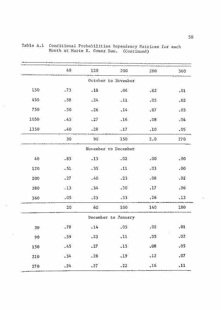
Table A.1 Conditional Probabilities Dependency Matrices for eachMonth at Marte R. Gomez Dam. (Continued)

40 120 200 280 360

October to November

150 .73 .18 .06 .02 .01

450 .58 .24 ,11 .05 .02

750 .50 .26 ,14 ,07 .03

1050 .45 .27 .16 .08 ,04

1350 .40 .28 .17 ,10 .05

30 90 150 2.0 270

November to December

40 .85 .13 ,02 .00 .00

120 .51 .35 ,11 .03 .00

200 .27 ,40 .23 .08 .02

280 .13 ,34 ,30 ,17 .06

360 .05 .23 .33 ,26 ,13

20 60 100 140 180

December to January

30 .78 .14 ,05 .02 .01

90 .59 .23 .11 ,05 .02

150 .45 .27 .15 ,08 .05

210 .34 .28 .19 ,12 ,07

270 .24 ,27 .22 ,16 ,11

APPENDIX B

COMPUTER PROGRAM

51

PROGRAM STOICO (INPUT,OUTPUT)******************v*.*********************************

IMPPOVED STOCHASTIC DYNAMIC FROGAMMINGOPTIMAL OPPATION POLICYMARTE R. GODEZ OAMOEXICO

4 ******************4*************444*******4

REAL IFCOMMON P( 5 .5,12).ST(11),INF(5,12),E(12),FTP1(11,5).

1 FT( 1. 1,5 ),FASTRI(1115),RASTRI(12,11,5),N,SMAX

NOTATION.P(I,J1K),TRANSITION PROBABILITY MATRIXK, IDENTIFY A PARTICULAR PAIR OF MONTHS.J.IDENTIFY THE DISCRETE VALUES OF INFLOWFOR PREVIOUS MONTH. •IIIDENTIFY THE DISCRETE VALUES OF INFLOWFOR CURRENT MONTH.ST,CONTAINS THE DISCRETE VALUES OF STORAGE(STATES)INF(I1J),CONTAINS THE DISCRETE VALUES OF INFLOWJ.IDENTIFY THE MONTH AND I A PARTICULAR VALUE.E(I),CONTAINS AMOUNTS OF EVAPORATION PER MONTH.ORT(I)ICONTAINS FOR EACH MONTH THE INCREMENT DESIREDFOR THE DECISION VARIABLE.NYEARSOUMBER OF CYCLES TO BE RUN THE MODEL.SMAX.UPPER LIMIT FOR STORAGE(CAPACITY OF THE DAM)SMIN,LOWER LIMIT OF STORAGE PERMISSIBLE.

***************************************** *****

READ DATA#444444*********************444 , 44***********

READ 50011((P(I.J,K)1I=1,5),J=1.5),K=1.12)READ 501.(ST(I),I=1.11)READ 502,((INF(I.J),I=115),J=1,12)READ 503,(E(I),I=1,12)READ 505,NYEARS,SMAX.SMTNORT.EPSILO*****************************************v**

INITIALIZE VALUES******************************************

DO 10 1=1,11DO 10 J=1.5FTP1(I1J1=0.0FT(I,J)=0.0FASTRI(I,J)=-999999999.9

1 0 CONTINUEFTP1(1115)=0.0ALPHA=rTP1(11,5)

w********************** ***** **************

DO FOR NUMBER OF YEARS AND TIME PERIODS444-***4**44*******************************

DO 70 ITT=1,NYEARSPRINT 507DO 50 I 1 =1,12*********444********************************

SET A FEASIdLE STATESET AN INITIAL STORAGE********************************************

DO 90 IST=1,11

52

PRINT 508***484444-4****444,444444444444444444444444444

SET A PREVIOUS INFLOW***********************************444444444

DO 20 ITM1=1,5#444444444444484,-*****###$#84 17.444444444444444

SET A FEASIBLE RELEASE*** 0-44 44#444, 8444#4-4444, $444 41-###44##4444444444

DO 30 IRT=1,21IRTT=IRT-1RT=IRTT*ORTPROD=0.0********************************************

FOR EACH CURRENTE INFLOW COMPUTE=(1) END STORAGE(2) EXPECTED VALUE OF ENO STORAGE(3) VALUE OF CURRENT ACTION***47.44*************************************4

DO 40 IIT=1,5STP1=ST(IST)+INF(IIT,IT)-RT-E(IT)IF(STP1.GT.SMAX) 305,396

305 STP1=SMAXGO TO 397

396 IF(STP1.LT.SMIN) GO TO 31397 ENT=STP1/100.- NIND=INT(ENT)

NINDI=NIND+1FX=FTP14NIND,IIT)+(ENT-NINO)*(FTP1(NINDI I IIT)-1FTP1(NINO,IIT))PROD=PROO+P(IIT,ITMi,IT)*FX

40 CONTINUEVR=52500.0-1.75*(RT-200.0)"2********************************************

COMPUTE SUM OF VALUE OF CURRENT ACTIONPLUS EXPECTED VALUE OF END STORAGE***********************************444444444

FT(IST,ITM1)=VR+PROD444444444444*444****************************

IS THIS SUM GREATER THAN THE PREVIOUSSUM COMPUTEDYES,STORE THIS SUM AND RELEASE DECISIONNO,DEFINE A NEW RELEASE************************** ********* ** ****** *

IF(FT(IST,ITM1).GT.FASTRI(IST I ITM1)) 1274,301274 FASTRI(IST,ITM1)=FT(IST,ITM1)

RASTRI(IT,IST,ITM1)=RT30 CONTINUE31 PRINT 506,IST,ITM1,FASTRI(IST,ITM1)*

1RASTRI(IT,IST,ITM1),IT20 CONTINUE

******************* ***** ************, *******

HAVE ALL POSSIBLE INITIAL STATES BEEN ANALYZED'********************************* ***** ******

90 CONTINUEDO 782 IST=1,11DO 782 ITM1=1,5FTP1(IST,ITM1)=FASTRI(IST,ITM1)

53

FT(IST,ITM1)=0.0FASTRI(IST.ITM1)=-999999999.9

782 CONTINUE50 CONTINUE

*****-v-*%, *************4,-**********************

HAVE OPTIMIZATION BEEN REACHED4***********1, ***44V**4************1-4*********

IF(A3S(FTP1(11,5)- ALPHA) .LE.EPSILO *ABS(FTP1(1115)))STOPDO 60 IST=1,11DO 60 ITM1=1,5FTP1(IST,ITM1)=FTP1(IST,ITM1)-FTP1(11,5)

60 CONTINUEIF(ITT.E0.1.0R.ITT.EQ.2) 61.62******4***************4*********************

ENTER SUBROUTINE FIXED********************************************

61 CALL FIXED62 ALPHA=FTP1(11,5)70 CONTINUE

500 FORMAT(5F10.2)501 FORMAT(fF10.2)502 FORMAT(5F10.2)503 FORMAT(6F10.0)504 FORMAT(6F10.0)505 FORMAT(I10,5F10.0)506 FORMAT(10X,*IST = 4- .I515X,*ITM1 =*115,5XOTASTRI =*,

1F10,0,5X,RASTRI =,F10.0,5X,MONTH = 1'915)507 FORMAT(1H1)508 FORMAT(1H )

END

54

SUBROUTINE FIXEDREAL INFCOMMON P(59r, 912),ST(11),INF(5912),E(12),FTP1(11,5),1FT(1195),FASTR,I(1195) 9 RASTR/(1291195),N9SMAXNCYCLES=1DO 70 ITT=19NCYCLESDO 50 IT=1,12********************4**************f********

SET A FEASIBLE STATESET AN INITIAL STORAGE*********44444444444#4444444444*************44

DO 90 IST=1,114*******M***********M**********44, 47V**,***4

SET A PREVIOUS INFLOW***********-t, *****4444******4444***444444444***

DO 20 ITM1=1 9 5PROD=0.******************************4****************

FOR EACH CURRENTE INFLOW COMPUTE=(1) END STORAGE(2) EXPECTED VALUE OF END STORAGE(3) VALUE OF CURRENT ACTIONMAKING USE OF THE SAME RELEASE DECISIONAS OBTAINED PREVIOUSLY'************;, *********4***********************

DO 40 IIT=195STP1=ST(IST)+INF(IIT9IT)*RASTRI(IT9IST9ITM1)-E(IT)IF(STP1.GT.SMAX) 305,397

305 STP1=SMAX397 ENT=STP1/100.

NIND=INT(ENT)NINDI=NIND+1FX=FTP1(NIND9IIT)+(ENT-NIND)*(FTPIANINDI9IIT) -

1FTP1(NIND 9 IIT))494.*******************41F**********************4

COMPUTE SUM OF VALUE OF CURRENT ACTIONPLUS EXPECTED VALUE OF END STORAGE** ***********49v******-m**IL****444m*********

PROD=PROD+P(IIT9ITM19IT)*FX

40 CONTINUEVR=52500.-1.75*(RASTRI(IT,IST9ITM1)-200.)"2F 1 (IST,ITM1)=VR+PROOPRINT 506 9 IST 9 ITM1 9 FT(IST 9 ITM1),RASTRI(ITIIST9ITM1),IT

20 CONTINUE*****************0***M**********************

HAVE ALL POSSIBLE INITIAL STATES BEEN ANALYZED******************************44494.4 ******* ****

90 CONTINUEDO 782 I 51 =19 1 1DO 782 ITM1=195FTP1(IST,ITM1)=FT(IST,ITM1)FT(IST 9 ITM1)=0.0

782 CONTINUE50 CONTINUE

DO 60 IST=1911DO 60 ITM1=195FTP1(IST 9 IT11)=FTP1(ISTIITM1)^FTP1(11.95)

55

60 CONTINUE70 CONTINUE

506 FORMAT(i0X,*IST =*,I5,5X,ITM1 =*II515X,*FASTRI1F10.Ù,5X,RASTRI =*,F10.0,5X,*1ONTH =',I51RETURNENO

56

REFERENCES

Askew, J. A., "Optimum Reservoir Operating Policies and theImposition of a Reliability Constraint", Water Resources Research, Vol. 10, No. 1, pp. 51-56, 1974.

Bellman, R. E„ Dynamic Programming, Princeton University Press,1957.

Clainos, D. M., Input Specifications to Stochastic Decision Models,M.S. Thesis, University of Arizona, Tucson, 1972.

Clainos, D. M., Roefs, T. G., Duckstein, L. "Creation of ConditionalDependency Matrices Based on a Stochastic Streamf low SynthesisTechnique", Water Resources Research, Vol. 9, No. 2, pp. 481-485,1973.

Harter, H. L„ "A New Table of Percentage Points of the Pearson Type3 Distributions", Technometrics, Vol. 11 (1), pp. 177-187,1969.

Hassitt, A., "Solution of the Stochastic Programming Model ofReservoir Regulation", Report No. 320-3506, 18 pp., IBMWashington Scientific Center, 1968,

Howard, R. A., Dynamic Programming and Markov Processes, M.I.T.Press, Cambridge, Mass., 1960.

Loucks, D. P., "Stochastic Methods for Analyzing River Basin Systems",Technical Report No. 16, Cornell University, Water Resources andMarine Sciences Center, Ithaca, N. Y., pp. V1-V21, 1969.

Loucks, D. P. and Falkson, L. M., "Comparison of some Dynamic, Linear,and Policy Iteration Methods for Reservoir Operation", Water Resources Bulletin, Vol. 6, No, 3, pp. 384-400, 1970.

MacQueen, J., "A Modified Dynamic Programming Method for MarkovianDecision Problems", J. Math , Anal. Appl., Vol. 14, pp, 38-43,1966.

Morton, T. E., "On the Asymptotic Convergence of Cost Differencesfor Markovian Decision Process", Operations Research, Vol. 19,pp. 244-249, 1971.

57

58

Odoni, A., "On Finding the Maximal Gain for Markov Decision Processes",Operations Research, Vol, 17, pp, 857-860, 1969*

Roefs, T. G., and Clainos, D. M., "Conditional Streamflow ProbabilityDistributions", in Hydrology and Water Resources in Arizona and the Southwest, Vol. 1, pp, 153-170, American Water ResourcesAssociation, Tucson, Arizona, 1971.

Roefs, T. G., Personal Communication, University of Arizona, Tucson,1974,

Schweitzer, P. J., "Perturbation Theory and Markovian DecisionProcesses", Operations Research Center, Technical ReportNo. 15, 1965.

Su, S. Y., and Deininger, R, A„ "Generalization of Whites Methodof Successive Approximations to Periodic Markovian DecisionProcesses", Operations Research, Vol, 20, No. 2, pp. 318-326,1972,

Vleugels, R. A., "Optimal Operation of Serially-Linked WaterReservoirs", Contribution No, 138, University of CaliforniaWater Resources Center, Los Angeles, Calif„ 54 pp. 1972.

White, D. J., "Dynamic Programming, Markov Chains and the Method ofSuccessive Approximations", J. Math. Anal. Appl„ Vol, 6,pp. 373-376, 1963.