PRUDENTIAL REGULATION AND BANK ACCOUNTING

i

PRUDENTIAL REGULATION AND BANK ACCOUNTING

A Dissertation

Presented to

The Faculty of the C.T. Bauer College of Business

University of Houston

In Partial Fulfillment

of the Requirements for the Degree

Doctor of Philosophy

By

Yan (Lanyi) Zhang

May 1st, 2019

ii

ACKNOWLEDGEMENTS

I would like to express my deep gratitude to my dissertation committee: Dr. Tong Lu,

Haijin Lin, Praveen Kumar, and Nisan Langberg, for their guidance, encouragement and

helpful critiques on this project. I particularly appreciate Dr. Tong Lu for his inspiration,

training and friendship in the past six years, which made my doctoral journey much more

fruitful and pleasant.

I thank all accounting faculties at the University of Houston, from whom I learned a lot. I

also thank all doctoral students at the accounting department, whose presence made our

accounting research much enjoyable.

I am grateful to the financial support provided by the University of Houston. It allowed me

to fully devote myself to accounting research and learn from other brilliant doctoral

students in the prestigious conferences.

I thank Xu Jiang, Jack Stecher, Haresh Sapra, Jonathan Glover, Urooj Khan and Hans

Frimor for their insightful comments and suggestions on this paper.

My deepest gratitude goes to my warm family, especially my daughter, Kathie, who has

been constantly providing me greatest motivation since her birth, and my parents who help

us take care of Kathie with their strongest supports and warmest loves in the whole process

of my doctoral study.

iii

PRUDENTIAL REGULATION AND BANK ACCOUNTING

Abstract of a Dissertation

Presented to

The Faculty of the C.T. Bauer College of Business

University of Houston

In Partial Fulfillment

of the Requirements for the Degree

Doctor of Philosophy

By

Yan (Lanyi) Zhang

May 1st, 2019

iv

ABSTRACT

This study focuses on how to design a mechanism that coordinates prudential regulation

and bank accounting. I study a setting in which a bank chooses its loan quality and makes

its asset substitution decision. The social planner sets the regulatory leverages for banks,

and the accounting regime (either fair value accounting or historical cost accounting) for

banks to report on loan performance. Using the ex ante bank value as the criterion, I find

that the historical cost regime dominates the fair value regime for medium values of asset

substitution risk; medium values of asset substitution constraint; low values of asset

specificity; low values of fundamental risk of loans; high values of marginal benefit or low

values of marginal cost of loan quality; and high values of the liquidity benefit of bank

debtholders. Fair value accounting dominates for other values of these parameters. This

study contributes to the theoretical literature on the debate about bank opacity by

incorporating both the asset side and the liability side of bank's balance sheets in designing

a mechanism to coordinate prudential regulation and bank accounting. The paper makes

important policy implications on prudential regulation and bank accounting such as cycle-

contingent regulations, asset risk class-contingent regulations and country-contingent

accounting standard.

v

TABLE OF CONTENTS

ACKNOWLEDGEMENTS ……………………………………………………..……... .ii

ABSTRACT ………………………………………………………………………....…..iv

LIST OF APPENDIX ………………………………………………………………….. vi

CHAPTER 1: INTRODUCTION ………………………………………………............. 1

CHAPTER 2: MODEL…………………………………………… ………………......... 9

2.1 Loan Portfolio………………………… ……………………………………………..9

2.2 Prudential Regulation and Bank Accounting………………………………………..10

2.3 Timeline… …………………………………………………………………………..12

2.4 Payoffs.. … …………………………………………………………………….........13

2.5 Endogenous and Exogenous Variables………………………………………………14

CHAPTER 3: PRUDENTIAL REGULATIONS UNDER HISTORICAL COST

ACCOUNTING………………………….………………………………………………..…16

CHAPTER 4: PRUDENTIAL REGULATIONS UNDER FAIR VALUE

ACCOUNTING ……………………………………………………………………............. 21

CHAPTER 5: HISTORICAL COST ACCOUNTING VERSUS FAIR VALUE

ACCOUNTING…………………………………………………………………………….. 26

5.1 Asset Substitution Risk and Constraint…………………………………………….. 26

5.2 Asset Specificity………………………………………………………………..…... 31

5.3 Fundamental Risk…………………………………………………………..………..33

5.4 Quality Level and Quality Cost…...……………………………………………..…..33

5.5 Liquidity Benefit……………………………………………………………….….....35

CHAPTER 6: CONCLUSIONS.………………………………………………………...38

vi

LIST OF APPENDIX

Proof of proposition 1……………………………………………………………….. 40




Proof of proposition 5…………………………………………………………….......42

Proof of the incremental effect of asset substitution on loan quality……….……...43

Proof of proposition 6………………………………………………………………...46




Proof of proposition 10 ..……………………………………………………………..51

CHAPTER 1

INTRODUCTION

Debates are ongoing on alternative �nancial accounting standards for banks, es-

pecially �nancial reporting opacity, in the context of prudential regulation of banks

(Laux and Leuz 2009). Prudential regulations are reformed period by period, such

as Basel I\Basel II\Basel III and mandatory stress test under Dodd-Frank Act, espe-

cially after the 2007-2009 �nancial crisis, which spawned a vigorous debate on the role

of bank regulation (Admati and Hellwig 2013, Gale 2010). Such prudential regulation

is accounting-based, for example prudential leverage ratios, which is de�ned as the

ratio of liability over asset of banks. Therefore, naturally a coordination of prudential

regulation and bank accounting is necessary to enhance social welfare.

Some argue for the importance of the asset side of bank's balance sheets. For

example, Morgan (2002, p. 874) states that �the opacity of banks exposes the entire

�nancial system to bank runs, contagion, and other strains of 'systemic' risk. Take

away opacity and the whole story unravels.� Similarly, Nier and Bauman (2006, p.

337) believe that �a bank that discloses its risk pro�le exposes itself to market dis-

cipline and will therefore be penalized by investors for choosing higher risk.� There-

fore, this type of views support fair value accounting, which reports timely interim

performance of bank's loan portfolios, thereby making it feasible for the prudential

regulators to �ne-tune the regulatory target leverages to precisely control the bank's

asset substitution (or risk shifting) decisions. That is, fair value accounting makes it

feasible for regulator to discipline bank's excessive risk taking, which may eventually

result in systemic risk.

However, others argue for the importance of the liability side of bank's balance

sheets. They emphasize the role of banks in the economy in creating highly liquid,

money-like debt claims (for example, demand deposits and the associated banking

1

services). Such claims are collateralized to make them information-insensitive. To

further make them information-insensitive, they argue, banks should be �secret keep-

ers,� and thus governmental guarantees, and regulation and supervision should not

force banks to publicly reveal information (Dang et al. 2014; Holmstöm 2015). There-

fore, this type of views support historical cost accounting, which does not report the

interim performance of bank's loan portfolios on a timely basis, thereby avoiding

triggering interim insolvency risk and thus safeguarding debtholders' deposits and

enhancing the debtholders' liquidity bene�ts.

I incorporate both the asset side and the liability side of bank's balance sheets

to investigate how the social planner coordinates prudential regulations and bank

accounting to enhance the ex ante bank value (the sum of the bank's ex ante debt

value and equity value). How should the optimal regulatory leverages be set, given a

particular accounting regime (fair value accounting versus historical cost accounting)

in place? Under what conditions will one accounting regime dominate the other? I

address these questions in a setting in which a representative bank chooses its loan

quality and makes its asset substitution decision.

Banks are plagued with debt overhang problems, including both asset substitu-

tion (or risk shifting) and underinvestment in loan quality. Banks may increase the

risk of its loan portfolios to gamble for the upside potential at the expense of the

debtholders, and the expected net present value su�ers as a result. For example,

they may undertake negative net present value projects (Jensen and Meckling 1976;

Dewatripont and Tirole 1993; Gron and Winton 2001; Admati and Hellwig 2013), or

they may construct derivatives for speculations based on the loan portfolios, or reduce

the frequency of �led inspection to the facility of borrowers in the hope of achieving

upside potential. Banks with excessive leverage may forgo positive net present value

projects and thus lead to under investment in the quality of the loan portfolios (Myers

1977; Admati et al. 2012).

2

I incorporate these two debt overhang problems in a two-period model charac-

terized by maturity mismatch, a prominent feature in the banking industry: The

bank �nances its long-term investment in loans (its largest asset items) using short-

term deposits (its largest liability items). Speci�cally, the bank chooses the quality

of its loan portfolios in period 1 and makes its asset substitution decision in period

2. Asset substitution in period 2 may enhance the bank's equity value in period 2;

Anticipating this, the bank is incentivized to choose a higher quality level for its loan

portfolios in period 1. Put it the other way, if the bank's period 2 asset substitution

is constrained, its period 1 incentive for quality will be dampened (Lu, Sapra, and

Subramanian 2019).

Apparently, the higher the bank leverage, the more incentivized the bank will

engage in asset substitution. Thus, it may seem naturally that the regulator may want

to lower the regulatory target leverage in period 2 to constrain asset substitution.

However, this will reduce the bank's incentive for quality, as discussed above. To

counteract this e�ect, the regulator may lower the regulatory target leverage in period

1 to reduce the debt overhang on the bank with respect to loan quality. If so, the

regulatory target leverages in both periods are lowered and thus the bank's debt

capacity is reduced, which implies lower liquidity bene�ts for the debtholders (Bryant

1980; Diamond and Dybvig 1983; Calomiris and Kahn 1991; Gale 2010).

I capture such economic tradeo�s in my model, and more importantly, I introduce

an accounting tradeo� (fair value accounting versus historical cost accounting). Un-

der fair value accounting in which the interim loan performance is reported, the bank

regulator can tie her interim prudential leverage to the fair value report and there-

fore can precisely curb or forbear bank's asset substitution (Giammarino, Lewis, and

Sappington 1993; Kahn and Winton 2004; Allen, Carletti, ad Marquez 2011; Bulow,

Gold�eld, and Klemperer 2013). However, the interim fair value report introduces

the interim volatility into the market value of bank debt and equity, thereby entailing

3

interim insolvency risk. Under historical cost accounting in which the loan perfor-

mance is not reported on a timely basis, the bank regulator cannot precisely control

bank's asset substitution due to the less informative accounting report. However, the

absence of timely fair value reports implies no interim volatility in the market value

of bank debt and equity, which suppresses the interim insolvency risk. 1

The main ingredients of the model are (1) bank's asset substitution and quality of

loan portfolios (the asset side of the bank's balance sheet) and (2) the bank debthold-

ers' liquidity bene�t (the liability side of the balance sheet), (3) the regulatory target

leverages for banks (prudential regulation), and (4) historical cost accounting versus

fair value accounting (bank accounting).

In my paper, bank value is de�ned as the sum of debt value plus equity value,

hence, both bank assets and bank liabilities are important for bank value. Therefore,

my main results are on the conditions under which one accounting regime dominates

the other in terms of the parameters of bank assets and liabilities, using the ex ante

bank value as the criterion. I �nd that the historical cost accounting regime dominates

the fair value accounting regime for the following parameter values of bank assets:

medium values of asset substitution risk; medium values of asset substitution con-

straint; low values of asset speci�city; high values of marginal bene�t or low values of

marginal cost of loan quality; low values of fundamental risk of loan portfolios. Histor-

ical cost accounting also dominates fair value accounting for the following parameter

value of bank liabilities: high values of the liquidity bene�t of bank debtholders. For

other parameter values, the fair value accounting regime dominates the historical cost

accounting regime.

My investigation contributes to the public policy debate on prudential regulation

1This paper study two pure accounting regime for bank loans, Fair value accounting and historicalcost accounting. The fair value of bank loan is level 3 fair value, which is determined by bank'sprivate information. Therefore, under historical cost accounting, as private information about loansis not incorporated into loan interim fair value and accounting report, accounting report on bankloans is less informative than that under fair value accounting. Here, I don't consider any manager'sdiscretion, because I study accounting standard setting.

4

and bank accounting.

(1) The social planner may condition her regulatory leverages and accounting

choice on the asset substitution risk classes of bank loans and/or the strength of

bank's corporate governance. For bank loans with extremely low or extremely high

asset substitution risk, fair value accounting is preferable, whereas for loans with

medium risk, historical cost accounting is called for. Furthermore, to the extent that

the asset substitution risk varies with the phases of business and credit cycles, my

result argues for cycle-contingent regulation, if practical. Speci�cally, to the extent

that the asset substitution risk is high in peak, low in trough and medium in con-

traction or expansion, it is optimal to implement fair value accounting in the peak

and trough phases of the cycle and historical cost accounting in the expansion and

contraction phases. With respect to corporate governance, my results argue for cor-

porate governance contingent regulation, if practical. Speci�cally, to the extent that

the asset substitution constraint is high for banks with good corporate governance,

for banks with bad corporate governance and medium for banks with medium corpo-

rate governance, it is optimal to implement fair value accounting for banks with good

or bad corporate governance and historical cost accounting for banks with medium

corporate governance.

(2) Fair value accounting is optimal for bank assets with high speci�city or high

illiquidity and historical cost accounting is optimal for generic assets or liquid assets.

Plantin, Sapra, and Shin (2008) generate an opposite result in a setting of premature

asset sales triggered by higher-order beliefs. Therefore, I identify another rationale

regarding the desirability of historical cost accounting versus fair value accounting in

terms of speci�city of bank assets.

(3) One of my results sheds light on impairment accounting (or lower-of-cost-or-

market rule). To the extent that the marginal bene�t (cost) of loan quality is high

(low) in good times and the converse is true in bad times, it is socially optimal to

5

mandate historical cost accounting in good times and fair value accounting in bad

times. This is what impairment accounting prescribes. Therefore, I adds bene�t of

the impairment accounting to the literature (Göx and Wagenhofer 2009; Li 2017),

which identify the bene�ts of impairment accounting to borrowers by exploring that

impairment accounting is bene�cial to lenders (banks).

(4) Another result is on liquidity bene�ts to bank depositors. To the extent that

depositors in developing countries value liquidity bene�ts relatively more than those

in developed countries, my result implies that historical cost accounting is better for

developing countries while fair value accounting is better for developed countries.

This implication warns developing countries against their rush to converge their local

accounting standards to the International Financial Reporting Standards, which are

taking great strides towards fair value accounting.

Overall, my study identi�es the characteristics of bank assets and liabilities that

should be taken into account in the mechanism design of prudential regulation and

bank accounting. In addition, it provides speci�c examples of how the two regulations

should be optimally coordinated.

My study contributes to the theoretical literature on bank accounting. (1) This

study incorporates both the asset side and the liability side of bank's balance sheets

to shed light on the debate over bank opacity. (2) This study focuses on regulatory

coordinations: How are prudential regulation and bank accounting optimally coordi-

nated?

Li (2017) and Bertomeu, Mahieux, and Sapra (2018) also study the coordination

of prudential regulation and bank accounting. Their focuses are di�erent from mine.

Li (2017) introduces capital issuance decision whereas Bertomeu, Mahieux, and Sapra

(2018) introduce accounting information system design, and both papers study the

loan risk decision. In contrast, I introduce bank's loan quality decision, which a�ect

both the mean and variance of loan fundamental.

6

Several papers focus on prudential regulation under fair value accounting only,

leaving out historical cost accounting. Heaton, Lucas, and McDonald (2010) inves-

tigate how to design capital requirements under mark-to-market regime. Lu, Sapra,

and Subramanian (2018) study a setting in which the bank can misreport its per-

formance under fair value accounting. In contrast, I extend and modify their model

and study historical cost accounting as well as fair value accounting, and thus pro-

vide a full picture regarding the optimal accounting choices for banks under di�erent

conditions.

Most existing accounting studies do not introduce or endogenize prudential regu-

lation. Allen and Carletti (2008) focus on historical cost versus fair value accounting

as well. In contrast to this study, they are interested in contagion from the insurance

sector to the banking sector. Plantin, Sapra, and Shin (2008) also focus on historical

cost versus fair value accounting for banks. They are interested in bank's asset sales

decision. Burkhardt and Strausz (2009) focus on historical cost versus impairment

accounting on asset substitution. In contrast, I introduce bank's quality decision as

well as asset substitution decision, thereby introducing the tradeo� between the two.

Corona, Nan, and Zhang (2018) focus on historical cost versus fair value accounting

for assets in place. They are interested in bank's lending decision as opposed to bank's

asset substitution and quality decisions, which are the key ingredients of my study.

In addition, they investigate bank's voluntary choice of accounting regimes whereas

I study mandatory accounting. Bleck and Gao (2018) compare the two accounting

regimes and study the loan selling decision assuming the prudential regulation (capital

requirement) is exogenous.2

My paper makes some empirical predictions. For example, the cycle-contingent or

asset risk class contingent regulations, corporate governance contenting regulations,

asset speci�city contingent accounting method, loan quality contingent accounting

2Some papers focus on other attributes of accounting as opposed to historical cost versus fairvalue accounting. For example, Corona, Nan, and Zhang (2015) focus on accounting quality.

7

method, country conditional accounting method. By developing proper proxy for the

parameters in my model, future empirical research can practically test my theoretical

results.

Section 2 describes the model setup. Section 3 analyzes the historical cost regime

and Section 4 analyzes the fair value regime. Section 5 compares the two regimes. The

proofs of Propositions are contained in the Appendix. Section 6 discusses potential

research extensions and summarizes this study.

8

CHAPTER 2

MODEL

I study a banking setting in which (i) a representative bank chooses the quality

(q) of its loan portfolios in period 1 and makes its asset substitution decision (a) in

period 2; (ii) a social planner chooses regulatory target leverages (equivalently, capital

requirements) for period 1 (L1) and period 2 (L2)3 and an accounting regime (fair

value accounting versus historical cost accounting). I modify and extend the model

in Lu, Sapra, and Subramanian (2018).

2.1 Loan Portfolio

At date 0, a representative bank originates a loan portfolio whose terminal cash

�ow V will be realized at date 2, V = XZ. Bank's two decisions will a�ect V : a

date 0 quality decision q ∈ {qH , qL} that will a�ect X and a date 1 asset substitution

decision a ∈ {0, 1} that will a�ect Z.

At date 0, the bank can engage in costly loan screening processes to �lter its loan

applications. The cost of quality is C(q) where C(q) = c if q = qH and C(q) = 0

if q = qL. The higher quality qH will generate a higher interim loan performance X

and thus a higher net present value. Hence, qH is more desirable than qL from the

perspective of the size of the pie. Speci�cally, X ∼ Lognormal(q, σ2X) with density

g(X) and cumulative distribution function G(X). Equivalently, X = eq+σXε where

ε ∼ N(0, 1). σX captures the fundamental risk of loan portfolio, that is: how volatile

the loan fundamental is. For example, the loan �nancing on �rm's R&D project is

more risky than the loan on other projects. I assume (eqH − eqL) e12σ2X > c , which

implies that the marginal bene�t of the higher quality qH relative to qL exceeds the

marginal cost. Naturally, the higher quality qH increases both the mean and the

3This is not a dynamic model to deal with multiple periods leverages, but rather ideally proposeleverages bundle as the socially optimal choice. The two leverages in my model represent thedi�erent prices for deposits in two di�erent periods; Practically, regulators do implement di�erentcapital requirement for di�erent economic conditions when needed, for example in recession period.

9

variance of X, which captures the idea that a higher expected return comes together

with a higher volatility.

At date 1, after privately learning the realized value of the interim loan per-

formance X, the bank can engage in asset substitution, for example, reducing the

frequency of its on-site inspections at borrower's facilities or increasing the riskiness

of the loan portfolio using derivatives. Speci�cally, Z ∼ Lognormal(−ak, a2σ2Z) with

density f(Z) and cumulative distribution function F (Z). Equivalently, Z = ea(σZη−k)

where η ∼ N(0, 1). σZ captures the asset substitution risk, that is: the opportunity

of the asset substitution or the upside potential for engaging in asset substitution.

For example, in peak, the opportunity of derivatives for speculation is relatively more

than in trough. k captures the constraint on asset substitution. For example, the

frequency of stress test, the soundness of corporate governance. I assume k > 12σ2Z

, which implies that asset substitution is very costly. Naturally, asset substitution

decreases the mean of Z and increases its variance and skewness, implying that asset

substitution on average is value-destroying.

2.2 Prudential Regulation and Bank Accounting

Bank industry has a very important feature, maturity mismatching. That is:

banks normally issue short-term deposits on the liability side and originate long-term

loans on the asset side of bank's balance sheet. On the asset side of the balance

sheet, because banks are highly levered, they are plagued with asset substitution and

underinvestment in loan quality. Speci�cally, because of high leverage, banks have

an incentive to use depositors' money to gamble for the upside potential, thereby ag-

gravating the asset substitution problem, which may damage loan NPV. In addition,

because of high leverage, the bulk of potential pro�ts from loan origination will be

accrued to depositors, but the cost of loan screening is borne by shareholders. There-

fore, banks are disincentivized to engage in costly loan quality investment, which

will also damage loan NPV. On the liability side of the balance sheet, banks' role

10

of providing liquidity bene�ts to depositors is crucial to social welfare. The higher

leverage, the more deposits will be issued, and the more associated liquidity bene�ts

will be. Hence, the insolvency risk of banks threatens the receipts of liquidity bene�ts

and deposits by depositors.4 Due to their weak bargaining power, individual depos-

itors cannot directly contract with banks to discipline bank's risk taking which will

a�ect the insolvency risk of banks. Bank regulator then steps in to represent indi-

vidual depositors to discipline bank's risk taking. Therefore, the banking industry is

characterized by strict regulations. For example, implement capital requirement and

stress test. Because neither asset substitution nor quality choice is veri�able, in this

paper, i focus on the leverage ratio, which is invoked by prudential regulation and is

well identi�ed in the literature to be the root of asset substitution problem and loan

quality incentive problem.

Because the bank chooses its loan quality in period 1 and makes its asset sub-

stitution decision in period 2, a social planner will ideally set a prudential leverage

for each period, {L1, L2}. Moreover, because of the maturity mismatching, that is,

banks use short-term deposits to �nance its long-term loans, the size of the deposits

(or the price of deposits) in periods 1 and 2 may be di�erent.5 This further enhances

the desirability of time-varying leverage ratios (as opposed to a �xed ratio for all

periods).

Because prudential leverage ratios are based on bank's balance sheet data, bank

accounting plays a critical role in bank regulations. The ongoing debate on historical

cost accounting versus fair value accounting is a case in point. Speci�cally, at date 1,

fair value accounting mandates interim loan performance reports, that is, the bank's

private information of the realized value of X.6 Thus, the social planner can tie pe-

4Deposit insurance by the Federal Deposit Insurance Corporation covers only a limited amountof deposits. My model setup is relevant as long as the depositors' loss exceeds this limit, which isespecially acute in �nancial crises in which systemic risk threatens the whole banking sector.

5My assumption of short-term deposits is purely to highlight the maturity mismatch betweenbank's assets and liabilities. All my results hold with a mixture of long-term and short-term deposits.

6Because of the long-term nature of loans, the date 1 realized value of X is the bank's private

11

riod 2 prudential leverage L2 to the accounting report X. In contrast, historical cost

accounting does not mandate a report of X at date 1. Therefore, the prudential lever-

age for period 2 cannot be tied to the bank's interim performance. In a nutshell, fair

value accounting provides more information than historical cost accounting.7 How-

ever, because of the multiple frictions in the economy, that is, the interactions of asset

substitution, underinvestment, and liquidity bene�t provisions, it is not always true

that �the more, the merrier,� as to be shown in later sections.8

2.3 Timeline

Given the social planner's choices of prudential regulation {L1, L2} and bank

accounting (historical cost or fair value), the game plays out as follows:

Date 0 :

(i) The bank �nances the initial investment I via short term debt, D0, and equity,

E0. The debt matures at date 1 with maturity value L1.

(ii) The bank chooses the loan quality, q ∈ {qH , qL}, and incurs quality cost C(q).

Date 1 :

(i) The interim loan performance X is realized and is privately known to the bank.

It is disclosed under fair value accounting but not under historical cost accounting.

(ii) Denote the market values of the bank's debt and equity at date 1 before L1 is paid

as D1 and E1, respectively. If the bank is insolvent, i.e., D1 + E1 < L1, the bank is

information rather than cash �ows. The loan portfolio's cash �ow is not X but V = XZ, which willbe realized at date 2. In addition, because the realized value of X is hidden information, the fairvalue report of X is a Level 3 input in the fair value hierarchy.

7The only di�erence between the two accounting regimes is that fair value accounting reportsinterim loan performance on a timely basis while historical cost accounting does not. Both accountingregimes report the loan origination value at date 0 and loan realized value at date 2.

8To focus on bank's quality choice and asset substitution decision, I take the bank's scale oflending as given, that is, I assume a �xed amount of investment I in place at the beginning of thegame. The literature has investigated the scale of investment thoroughly (e.g., Corona, Nan, andZhang (2018)). As a consequence, I cannot deal with hybrid accounting regimes in this model. Forexample, an impairment accounting will mandate the disclosure of min{I,X} at date 1. To make itinteresting enough, my model must endogenize I before addressing the merits and demerits of im-pairment accounting. However, Proposition 9 in Section 5 does imply the desirability of impairmentaccounting, which is also summarized in the Introduction.

12

bankrupt and the liquidation value of the loan portfolio is normalized to be 0 because

the pre-mature project is low valued. If the bank is solvent, i.e., D1 + E1 ≥ L1, the

bank makes the required debt payment L1 by issuing new debt and (if necessary)

equity.9 The debt issued at date 1 will mature at date 2 with maturity value L2.

(iii) The bank makes its asset substitution decision a ∈ {0, 1}.

Date 2 :

(i) The terminal cash �ow of the bank's loan portfolio will be realized as V = XZ.

(ii) If the bank is insolvent, i.e., V < L2, the bank is bankrupt and the liquidation

value of the loan portfolio is αV where α ∈ (0, 1) and thus 1 − α represents asset

speci�city that causes the deadweight loss in liquidation. If the bank is solvent, i.e.,

V ≥ L2, the bank makes the required debt payment L2.10

2.4 Payo�s

At date 0, bank's depositors lend D0 to the bank, and the bank's shareholders

receive it and incur the cost of quality investment C(q), therefore, the net proceeds

received will be: D0 − C(q).

Because bank's depositors value the liquidity bene�ts, their payo�s consist of

not only the pecuniary amount (cash �ows from the bank) but also a non-pecuniary

bene�t, which is normally called liquidity bene�ts (also called �convenience spread� in

�nance literature). Hence, at date 1, if the bank is solvent (D1 +E1 ≥ L1), the period

1 depositors' payo� is L1(1 + λ), where λ represents the liquidity bene�t per dollar

deposits.11 The period 2 depositors lend D1 to the bank. Thus, bank shareholders'

9If the amount of new debt raised exceeds the required payment of the old debt, that is, ifD1 > L1, I assume that the bank will use the surplus as new equity. For example, the bank mayissue restricted stocks whose vesting date is date 2. The reason why I am assuming so is to makething easy. In practice, bank can pay dividends with the extra money. However, the paid dividendwill decrease the equity of bank. Therefore, the equity value after paying dividend at date 1 will haveto deduct the paid dividend, which is a constant number assumed. Deducting a constant numberwon't change the essence of my story. Therefore, I normalize the dividend paid as 0 to make mymodel mathematically easier.

10If loans are prematurely liquidated at date 1, their liquidate value will be much lower than atthe loan maturity date (date 2). To capture this di�erence, I normalize the date 1 liquidate valueto 0 and assume a positive liquidation value αV at date 2.

11Subramanian and Yang (2018) document that on average λ = 25% with a standard error of 0.08

13

payo� is D1 − L1. If the bank is insolvent, both depositors and shareholders will

receive nothing.

At date 2, if the bank is solvent (V ≥ L2), the period 2 depositors' payo� is

L2(1 + λ). Thus, bank shareholders' payo� is V − L2. If the bank is insolvent,

depositors' payo� is αV (1 + λ) and shareholders will receive nothing. I assume that

α(1 + λ) < 1 to avoid the unrealistic scenario in which the liquidation at date 2

generates a higher social value (αV (1 + λ) ) than the cash �ow without deadweight

loss (V ).

2.5 Endogenous and Exogenous Variables

I focus on the bank's date 0 loan quality choice q ∈ {qH , qL} and its date 1

asset substitution decision a ∈ {0, 1}. I assume that the social planner's objective

is to maximize the date 0 bank value, that is, π0 ≡ D0 + E0, the sum of the date

0 debt value and equity value of the bank, and the bank's objective is to maximize

equity value at each date. Given these objectives, I investigate the social planner's

optimal choices of prudential leverages for periods 1 and 2, that is, {L1, L2}, under

an accounting regime in place, historical cost accounting or fair value accounting,

to induce bank's decision on loan quality and asset substitution. I will identify the

conditions under which one accounting regime dominates the other. Eventually, I will

show how to design the optimal coordination mechanisms for prudential regulation

and bank accounting to enhance bank value.

I am interested in several parameters in economic environments that shed light

on the optimal coordination of prudential regulation and bank accounting. On the

asset side of the bank's balance sheet, I am interested in two sets of parameters:

(i) those that a�ect the bank's quality decisions: σX (fundamental risk of the

loan portfolio); qH relative to qL (the incremental bene�t of loan quality); and c (the

incremental cost of loan quality).

for banks in the U.S. over the period of 1991 to 2008.

14

(ii) those that a�ect the bank's asset substitution decision: σZ (asset substitution

risk); k (asset substitution constraint); and 1 − α (the deadweight loss due to the

date 2 insolvency caused by asset speci�city).

On the liability side of the bank's balance sheet, I am interested in the parameter

λ (liquidity bene�t to depositors).

15

CHAPTER 3

PRUDENTIAL REGULATIONS UNDER HISTORICAL

COST ACCOUNTING

Under historical cost accounting, interim loan performance X is not publicly dis-

closed at date 1. However, the bank has private knowledge about X. At date 1, the

bank chooses its asset substitution decision to maximize its date 2 expected payo�,

given its private knowledge of the realized interim loan performance X:

maxa

E [1V≥L2 • (V − L2)|X] , (1)

where the bank will be solvent when its date 2 bank value V exceeds its date 2

obligation L2 and 1V≥L2 is an indicator function that equals 1 if V ≥ L2 and 0

otherwise.

The following proposition con�rms the conventional wisdom that high leverage

leads to asset substitution.

Proposition 1. (a) At date 1, the bank will choose asset substitution (a = 1) over

no asset substitution (a = 0) if and only if the leverage is high enough (L2 > γ0X).

(b) At date 1, the date 2 insolvency risk is F(L2

X

).

In the above, γ0 is de�ned by

1− γ0 =

∞̂

γ0

(Z − γ0) f(Z)dZ. (2)

At date 1, market values of equity and debt are, respectively,

E1 = E [1V≥L2 • (V − L2)]

D1 = E [1V≥L2 • L2(1 + λ) + 1V <L2 • αV (1 + λ)], (3)

16

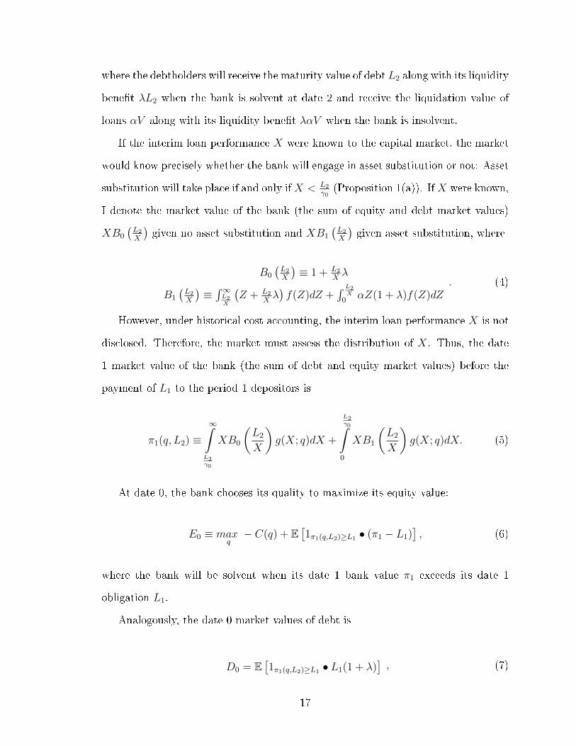
where the debtholders will receive the maturity value of debt L2 along with its liquidity

bene�t λL2 when the bank is solvent at date 2 and receive the liquidation value of

loans αV along with its liquidity bene�t λαV when the bank is insolvent.

If the interim loan performance X were known to the capital market, the market

would know precisely whether the bank will engage in asset substitution or not: Asset

substitution will take place if and only ifX < L2

γ0(Proposition 1(a)). IfX were known,

I denote the market value of the bank (the sum of equity and debt market values)

XB0

(L2

X

)given no asset substitution and XB1

(L2

X

)given asset substitution, where

B0

(L2

X

)≡ 1 + L2

Xλ

B1

(L2

X

)≡´∞L2X

(Z + L2

Xλ)f(Z)dZ +

´ L2X

0αZ(1 + λ)f(Z)dZ

. (4)

However, under historical cost accounting, the interim loan performance X is not

disclosed. Therefore, the market must assess the distribution of X. Thus, the date

1 market value of the bank (the sum of debt and equity market values) before the

payment of L1 to the period 1 depositors is

π1(q, L2) ≡∞̂

L2γ0

XB0

(L2

X

)g(X; q)dX +

L2γ0ˆ

0

XB1

(L2

X

)g(X; q)dX. (5)

At date 0, the bank chooses its quality to maximize its equity value:

E0 ≡ maxq− C(q) + E

[1π1(q,L2)≥L1 • (π1 − L1)

], (6)

where the bank will be solvent when its date 1 bank value π1 exceeds its date 1

obligation L1.

Analogously, the date 0 market values of debt is

D0 = E[1π1(q,L2)≥L1 • L1(1 + λ)

], (7)

17

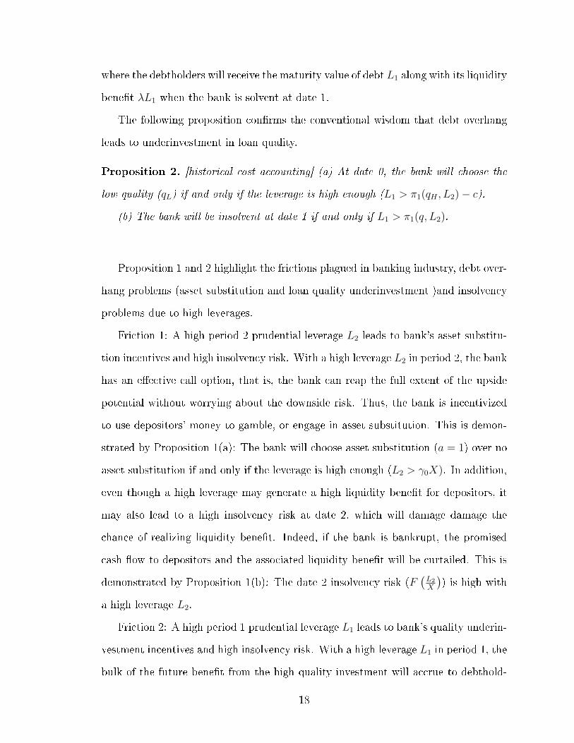
where the debtholders will receive the maturity value of debt L1 along with its liquidity

bene�t λL1 when the bank is solvent at date 1.

The following proposition con�rms the conventional wisdom that debt overhang

leads to underinvestment in loan quality.

Proposition 2. [historical cost accounting] (a) At date 0, the bank will choose the

low quality (qL) if and only if the leverage is high enough (L1 > π1(qH , L2)− c).

(b) The bank will be insolvent at date 1 if and only if L1 > π1(q, L2).

Proposition 1 and 2 highlight the frictions plagued in banking industry, debt over-

hang problems (asset substitution and loan quality underinvestment )and insolvency

problems due to high leverages.

Friction 1: A high period 2 prudential leverage L2 leads to bank's asset substitu-

tion incentives and high insolvency risk. With a high leverage L2 in period 2, the bank

has an e�ective call option, that is, the bank can reap the full extent of the upside

potential without worrying about the downside risk. Thus, the bank is incentivized

to use depositors' money to gamble, or engage in asset substitution. This is demon-

strated by Proposition 1(a): The bank will choose asset substitution (a = 1) over no

asset substitution if and only if the leverage is high enough (L2 > γ0X). In addition,

even though a high leverage may generate a high liquidity bene�t for depositors, it

may also lead to a high insolvency risk at date 2, which will damage damage the

chance of realizing liquidity bene�t. Indeed, if the bank is bankrupt, the promised

cash �ow to depositors and the associated liquidity bene�t will be curtailed. This is

demonstrated by Proposition 1(b): The date 2 insolvency risk (F(L2

X

)) is high with

a high leverage L2.

Friction 2: A high period 1 prudential leverage L1 leads to bank's quality underin-

vestment incentives and high insolvency risk. With a high leverage L1 in period 1, the

bulk of the future bene�t from the high quality investment will accrue to debthold-

18

ers. Thus, the bank is disincentivized to choose a costly quality investment. This is

demonstrated by Proposition 2(a): The bank will choose the low quality (qL) over

the high quality if and only if the leverage is high enough (L1 > π1(qH , L2) − c).

In addition, even though a high leverage may generate a high liquidity bene�t for

depositors, it may also lead to a high insolvency risk at date 1, which will damage

the chance of realizing liquidity bene�t. This is demonstrated by Proposition 2(b):

The bank will be insolvent if and only if L1 > π1(q, L2).

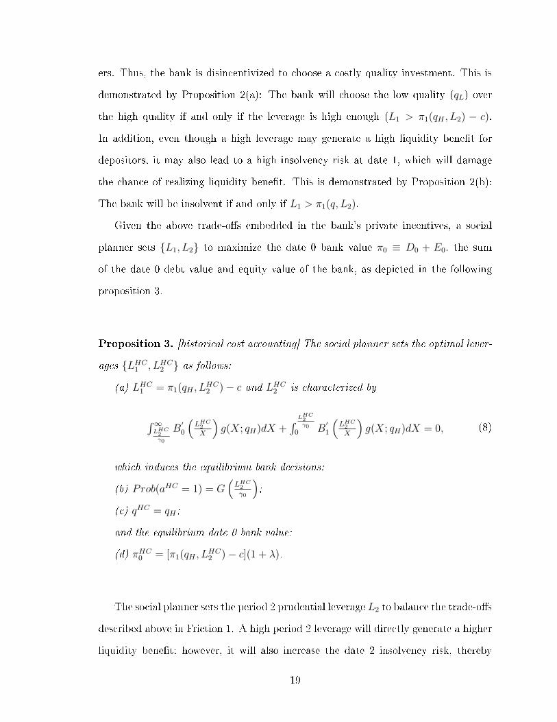
Given the above trade-o�s embedded in the bank's private incentives, a social

planner sets {L1, L2} to maximize the date 0 bank value π0 ≡ D0 + E0, the sum

of the date 0 debt value and equity value of the bank, as depicted in the following

proposition 3.

Proposition 3. [historical cost accounting] The social planner sets the optimal lever-

ages {LHC1 , LHC2 } as follows:

(a) LHC1 = π1(qH , LHC2 )− c and LHC2 is characterized by

´∞LHC2γ0

B′0

(LHC2

X

)g(X; qH)dX +

´ LHC2γ0

0 B′1

(LHC2

X

)g(X; qH)dX = 0, (8)

which induces the equilibrium bank decisions:

(b) Prob(aHC = 1) = G(LHC2

γ0

);

(c) qHC = qH ;

and the equilibrium date 0 bank value:

(d) πHC0 = [π1(qH , LHC2 )− c](1 + λ).

The social planner sets the period 2 prudential leverage L2 to balance the trade-o�s

described above in Friction 1. A high period 2 leverage will directly generate a higher

liquidity bene�t; however, it will also increase the date 2 insolvency risk, thereby

19

damaging the chance of realizing the liquidity bene�t in the �rst place. In addition, a

higher leverage will induce a higher incidence of asset substitution, which will decrease

the date 1 bank value. The balancing of these forces yields the optimal choice of L2

(equation (8)), which, in turn, determines the incidence of asset substitution targeted

by the social planner (Prob(aHC = 1) = G(LHC2

γ0

)).

The social planner also sets the period 1 prudential leverage L1 to balance the

trade-o�s described above in Friction 2. A high period 1 leverage will directly generate

a higher liquidity bene�t; however, it will also increase the date 1 insolvency risk,

thereby damaging the chance of realizing the liquidity bene�t in the �rst place. In

addition, a higher leverage will discourage the bank from choosing the high quality.

The balancing of these forces yields the optimal choice of L1, which, in turn, induces

the bank to choose the high quality (qHC = qH).

Because the social planner sets the prudential regulations {L1, L2} at the same

time at date 0, they are naturally optimally combined. Speci�cally, the social planner

sets L2 to maximize the date 1 bank value π1 before the payment of L1 to the period

1 depositors. Because a higher date 1 bank value encourages the bank's quality

investment, the period 1 debt overhang problem is mitigated, and thus the social

planner can push L1 up to enhance the period 1 liquidity bene�t to the fullest extent,

only constrained by the requirement that no interim insolvency will be triggered.12

12Under historical cost accounting, X is not disclosed, therefore, social planner cannot preciselyinduce the socially desirable bank's choice of asset substitution, but rather an optimal incidenceof asset substitution. In this regard, regulation is less e�cient compared to second-best regulationunder fair value accounting. With this third-best regulation on asset substitution, a social plannerhas to make sure high quality is �rst induced to enhance ex-ante bank value. This is why highquality is always induced under historical cost accounting.

20

CHAPTER 4

PRUDENTIAL REGULATIONS UNDER FAIR VALUE

ACCOUNTING

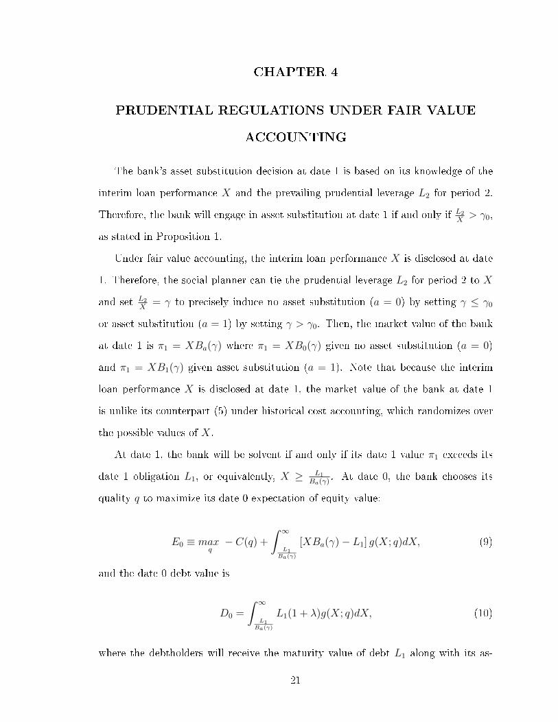
The bank's asset substitution decision at date 1 is based on its knowledge of the

interim loan performance X and the prevailing prudential leverage L2 for period 2.

Therefore, the bank will engage in asset substitution at date 1 if and only if L2

X> γ0,

as stated in Proposition 1.

Under fair value accounting, the interim loan performance X is disclosed at date

1. Therefore, the social planner can tie the prudential leverage L2 for period 2 to X

and set L2

X= γ to precisely induce no asset substitution (a = 0) by setting γ ≤ γ0

or asset substitution (a = 1) by setting γ > γ0. Then, the market value of the bank

at date 1 is π1 = XBa(γ) where π1 = XB0(γ) given no asset substitution (a = 0)

and π1 = XB1(γ) given asset substitution (a = 1). Note that because the interim

loan performance X is disclosed at date 1, the market value of the bank at date 1

is unlike its counterpart (5) under historical cost accounting, which randomizes over

the possible values of X.

At date 1, the bank will be solvent if and only if its date 1 value π1 exceeds its

date 1 obligation L1, or equivalently, X ≥ L1

Ba(γ). At date 0, the bank chooses its

quality q to maximize its date 0 expectation of equity value:

E0 ≡ maxq− C(q) +

ˆ ∞L1

Ba(γ)

[XBa(γ)− L1] g(X; q)dX, (9)

and the date 0 debt value is

D0 =

ˆ ∞L1

Ba(γ)

L1(1 + λ)g(X; q)dX, (10)

where the debtholders will receive the maturity value of debt L1 along with its as-

21

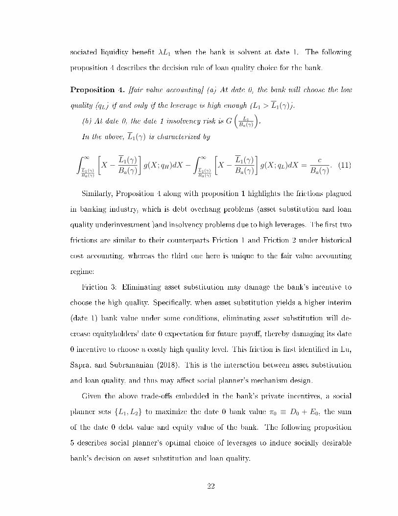
sociated liquidity bene�t λL1 when the bank is solvent at date 1. The following

proposition 4 describes the decision rule of loan quality choice for the bank.

Proposition 4. [fair value accounting] (a) At date 0, the bank will choose the low

quality (qL) if and only if the leverage is high enough (L1 > L1(γ)).

(b) At date 0, the date 1 insolvency risk is G(

L1

Ba(γ)

).

In the above, L1(γ) is characterized by

ˆ ∞L1(γ)Ba(γ)

[X − L1(γ)

Ba(γ)

]g(X; qH)dX −

ˆ ∞L1(γ)Ba(γ)

[X − L1(γ)

Ba(γ)

]g(X; qL)dX =

c

Ba(γ). (11)

Similarly, Proposition 4 along with proposition 1 highlights the frictions plagued

in banking industry, which is debt overhang problems (asset substitution and loan

quality underinvestment )and insolvency problems due to high leverages. The �rst two

frictions are similar to their counterparts Friction 1 and Friction 2 under historical

cost accounting, whereas the third one here is unique to the fair value accounting

regime:

Friction 3: Eliminating asset substitution may damage the bank's incentive to

choose the high quality. Speci�cally, when asset substitution yields a higher interim

(date 1) bank value under some conditions, eliminating asset substitution will de-

crease equityholders' date 0 expectation for future payo�, thereby damaging its date

0 incentive to choose a costly high quality level. This friction is �rst identi�ed in Lu,

Sapra, and Subramanian (2018). This is the interaction between asset substitution

and loan quality, and thus may a�ect social planner's mechanism design.

Given the above trade-o�s embedded in the bank's private incentives, a social

planner sets {L1, L2} to maximize the date 0 bank value π0 ≡ D0 + E0, the sum

of the date 0 debt value and equity value of the bank. The following proposition

5 describes social planner's optimal choice of leverages to induce socially desirable

bank's decision on asset substitution and loan quality.

22

Proposition 5. [fair value accounting] The social planner sets the optimal leverages

{LFV1 , LFV2 } as follows:

(i) If

A

(L1(γa)

Ba(γa), qH

)− A

(eqL+S, qL

)≥ c

Ba(γa), (12)

LFV1 = L1(γa) and LFV2 = γ0X if B0(γ0) ≥ B1(γ1) and LFV2 = γ1X if B1(γ1) >

B0(γ0),


qFV = qH ;

aFV = 0 if B0(γ0) ≥ B1(γ1) and aFV = 1 if B1(γ1) > B0(γ0);

the equilibrium date 0 bank value πFV0 = Ba(γa)A(L1(γa)Ba(γa)

, qH

)− c.

(ii) If A(L1(γa)Ba(γa)

, qH

)− A

(eqL+S, qL

)< c

Ba(γa),

LFV1 = eqL+SBa(γa) and LFV2 = γ0X if B0(γ0) ≥ B1(γ1) and LFV2 = γ1X if

B1(γ1) > B0(γ0),


qFV = qL;

aFV = 0 if B0(γ0) ≥ B1(γ1) and aFV = 1 if B1(γ1) > B0(γ0);

the equilibrium date 0 bank value πFV0 = Ba(γa)A(eqL+S, qL

).

In the above, A(

L1

Ba(γ), q)≡´∞

L1Ba(γ)

[X + L1

Ba(γ)λ]g(X; q)dX

and Ba(γa) = max{B0(γ0), B1(γ1)}, where

B0 (γ0) ≡ 1 + γ0λ

B1 (γ1) ≡´∞γ1

(Z + γ1λ) f(Z)dZ +´ γ10αZ(1 + λ)f(Z)dZ

, (13)

and

γ1 ≡ eT−k, (14)

where T is de�ned by h(T/σZ)/σZ = λ(1+λ)(1−α) and S is de�ned by h(S/σX)/σX =

λ1+λ

, in which h() is a hazard rate function for a standard normal distribution.

23

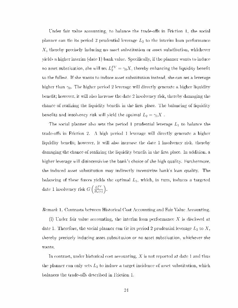
Under fair value accounting, to balance the trade-o�s in Friction 1, the social

planner can tie its period 2 prudential leverage L2 to the interim loan performance

X, thereby precisely inducing no asset substitution or asset substitution, whichever

yields a higher interim (date 1) bank value. Speci�cally, if the planner wants to induce

no asset substitution, she will set LFV2 = γ0X, thereby enhancing the liquidity bene�t

to the fullest. If she wants to induce asset substitution instead, she can set a leverage

higher than γ0. The higher period 2 leverage will directly generate a higher liquidity

bene�t; however, it will also increase the date 2 insolvency risk, thereby damaging the

chance of realizing the liquidity bene�t in the �rst place. The balancing of liquidity

bene�ts and insolvency risk will yield the optimal L2 = γ1X .

The social planner also sets the period 1 prudential leverage L1 to balance the

trade-o�s in Friction 2. A high period 1 leverage will directly generate a higher

liquidity bene�t; however, it will also increase the date 1 insolvency risk, thereby

damaging the chance of realizing the liquidity bene�t in the �rst place. In addition, a

higher leverage will disincentivize the bank's choice of the high quality. Furthermore,

the induced asset substitution may indirectly incentivize bank's loan quality. The

balancing of these forces yields the optimal L1, which, in turn, induces a targeted

date 1 insolvency risk G(LFV1

Ba(γ)

).

Remark 1. Contrasts between Historical Cost Accounting and Fair Value Accounting.

(i) Under fair value accounting, the interim loan performance X is disclosed at

date 1. Therefore, the social planner can tie its period 2 prudential leverage L2 to X,

thereby precisely inducing asset substitution or no asset substitution, whichever she

wants.

In contrast, under historical cost accounting, X is not reported at date 1 and thus

the planner can only sets L2 to induce a target incidence of asset substitution, which

balances the trade-o�s described in Friction 1.

24

(ii) Under historical cost accounting, the interim loan performance X is not dis-

closed at date 1 and thus no volatility in the interim (date 1) market value of the

bank exists. Therefore, even at date 0, the social planner can for certain induce the

interim solvency without any uncertainty. To do so, she sets her period 1 prudential

leverage L1 to induce the bank to choose the high quality to boost the date 1 bank

value.

In contrast, under fair value accounting, X is reported at date 1 and therefore

the interim (date 1) market value of the bank will be volatile, thereby potentially

triggering interim insolvency. Because at date 0 the social planner cannot know the

exact value of X to be disclosed at date 1, she sets L1 to induce a target incidence of

interim insolvency, which balances the trade-o�s described in Friction 2 and 3.

(iii) As a consequence of (i) and (ii), under historical cost accounting, the social

planner sets her prudential leverages to induce a target incidence of asset substitution

and the high quality level, whereas under fair value accounting, she sets her prudential

leverages to induce her desired level of asset substitution and a target incidence of

interim insolvency, which may engender the high or low quality level.

In particular, under fair value accounting, it is not surprising that under certain

parameter values, a combination of {a = 0, q = qH} which maximizes the net cash �ow

may occur in equilibrium. However, more interestingly, under other parameter values,

Friction 3 described above may take force: that is, eliminating asset substitution

may endanger the bank's quality investment (that is, a combination of {a = 0, q =

qL}), or on the other direction, forbearing asset substitution in order to boost the

bank's quality investment (that is, a combination of {a = 1, q = qH}) may occur in

equilibrium.13

13In my model, a social planner simultaneously chooses two optimal regulatory leverages to in-duce socially desirable bank's choice of asset substitution in period 2 and loan quality in period1. Therefore, asset substitution and loan quality are organically interacted with each other by twoleverages. To isolate how leverage induces desirable loan quality without considering the e�ect ofasset substitution on loan quality, that is, the e�ect of friction 3 described above, in the appendix, Iwill illustrate the incremental e�ect of asset substitution on loan quality in a hypothetical accounting

25

CHAPTER 5

HISTORICAL COST ACCOUNTING VERSUS FAIR

VALUE ACCOUNTING

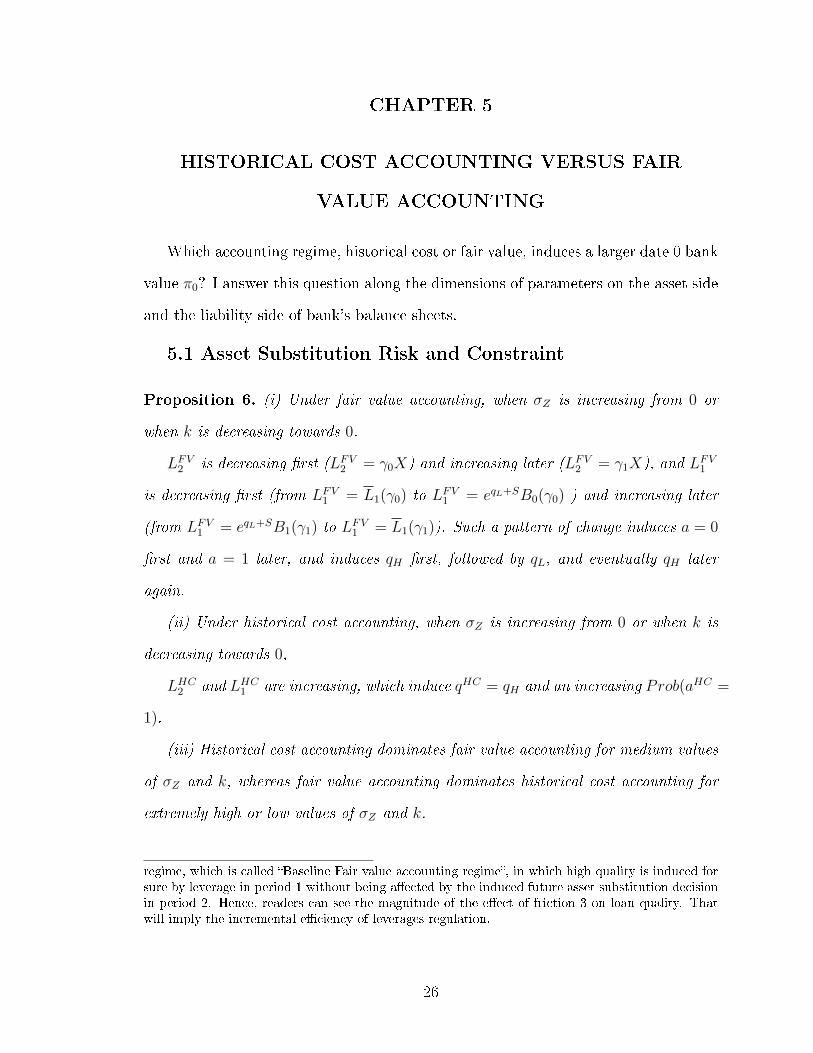
Which accounting regime, historical cost or fair value, induces a larger date 0 bank

value π0? I answer this question along the dimensions of parameters on the asset side

and the liability side of bank's balance sheets.

5.1 Asset Substitution Risk and Constraint

Proposition 6. (i) Under fair value accounting, when σZ is increasing from 0 or

when k is decreasing towards 0,

LFV2 is decreasing �rst (LFV2 = γ0X) and increasing later (LFV2 = γ1X), and LFV1

is decreasing �rst (from LFV1 = L1(γ0) to LFV1 = eqL+SB0(γ0) ) and increasing later

(from LFV1 = eqL+SB1(γ1) to LFV1 = L1(γ1)). Such a pattern of change induces a = 0

�rst and a = 1 later, and induces qH �rst, followed by qL, and eventually qH later

again.

(ii) Under historical cost accounting, when σZ is increasing from 0 or when k is

decreasing towards 0,

LHC2 and LHC1 are increasing, which induce qHC = qH and an increasing Prob(aHC =

1).

(iii) Historical cost accounting dominates fair value accounting for medium values

of σZ and k, whereas fair value accounting dominates historical cost accounting for

extremely high or low values of σZ and k.

regime, which is called �Baseline Fair value accounting regime�, in which high quality is induced forsure by leverage in period 1 without being a�ected by the induced future asset substitution decisionin period 2. Hence, readers can see the magnitude of the e�ect of friction 3 on loan quality. Thatwill imply the incremental e�ciency of leverages regulation.

26

A higher asset substitution risk σZ or a looser asset substitution constraint k

motivates bank's asset substitution incentives. Therefore, in the following, I focus

on the intuition of Proposition 6 in terms of σZ with the understanding that the

same intuition applies for k. The frictions I introduced before feature strongly in

Proposition 6.

Under fair value accounting, when asset substitution risk σZ is extremely low,

asset substitution is not quite attractive to the bank in the �rst place. Therefore, the

social planner can comfortably set high prudential leverage LFV2 to induce no asset

substitution without ever compromising liquidity bene�ts to depositors. The high

leverage in period 2 with induced no asset substitution will boost the interim bank

value, which will give social planner ample room to set a high leverage LFV1 to induce

high quality of loans.

When asset substitution risk σZ is increasing, the bank's asset substitution incen-

tive is increasing. Therefore, to curb bank's increasing incentive of asset substitution,

the social planner lowers the period 2 prudential leverage LFV2 . However, because

of the trade-o� described in Friction 3, a dampened asset substitution incentive will

disincentivize the bank's quality investment. To restore the high quality, the so-

cial planner will lower the period 1 prudential leverage LFV1 to reduce debt overhang.

Although both no asset substitution and high quality are induced, it comes at the

expense of lower liquidity bene�ts implied by lower prudential leverages. Therefore,

the date 0 bank value decreases.

When asset substitution risk σZ increases further, the induced low quality in-

centive alluded to above becomes even stronger. Further decreasing leverage LFV1 to

induce high quality becomes too costly. Therefore, the social planner has to toler-

ate the low quality, which leads to a high chance of the interim (date 1) insolvency

risk. To control this heightened risk, the social planner further lowers the period 1

prudential leverage L1. The low quality qL in conjunction with low leverages further

27

decreases the date 0 bank value.

When asset substitution risk σZ increases even further, lowering L2 further would

sacri�ce too many liquidity bene�ts. Therefore, the social planner increases L2 to

forbear asset substitution. At the same time, a higher level of L2 implies a higher

level of liquidity bene�ts and thus a higher interim (date 1) bank value. A higher bank

value at date 1 reduces the interim insolvency risk and thus gives the social planner

ample room to increase the period 1 prudential leverage L1 to enhance the period 1

liquidity bene�t. For these reasons, the date 0 bank value reverses its downward slip

and starts to increase.

When asset substitution risk σZ continues to increase further, the force of Friction

3 works to its fullest extent: An ever-increasing period 2 asset substitution incentive

will eventually induce the bank to choose the high quality in period 1. This gives the

social planner ample room to increase the period 1 prudential leverage L1 to enhance

the period 1 liquidity bene�t. For these reasons, the date 0 bank value increases even

more.

Under historical cost accounting, because the interim loan performance X is not

disclosed, the social planner cannot eliminate asset substitution for certain because

it cannot �ne-tune its period 2 prudential leverage L2 to X. In other words, she has

to allow for a probability of asset substitution. Therefore, the higher the value of

σZ , the higher incentive of asset substitution, and then the high incidence of asset

substitution. To induce an increasing optimal incidence of asset substitution, the

higher the level of LHC2 will be set by the social planner. At the same time, a higher

level of L2 implies a higher level of liquidity bene�ts and thus a higher interim (date

1) bank value. A higher bank value at date 1 reduces the interim insolvency risk and

thus gives the social planner ample room to increase the period 1 prudential leverage

L1 to enhance the period 1 liquidity bene�t. For these reasons, the date 0 bank value

increases.

28

Which accounting regime, historical cost or fair value, induces a higher date 0

bank value?

Proposition 6(iii) provides the answer: Historical cost accounting dominates fair

value accounting for medium values of asset substitution risk and constraint, and fair

value accounting dominates for extremely high or low values. The intuition behind

this result hinges crucially upon Frictions 1, 2, and 3 described before and the fact that

the prudential leverages L1 and L2 are optimally coordinated by the social planner.

When asset substitution risk σZ is extremely low, the curbed asset substitution

with high leverage L2 results in the higher interim bank value and the lower interim

insolvency risk under fair value accounting than under historical cost accounting; the

social planner can thus take advantage of it to boost L1 to enhance liquidity bene�ts.

Therefore, the date 0 bank value under fair value accounting is higher than under

historical cost accounting in this σZ area.

By the same token, when asset substitution risk σZ is extremely high, the tolerated

asset substitution with high leverage L2 results in the higher interim bank value and

the lower interim insolvency risk under fair value accounting than under historical cost

accounting; the social planner can thus take advantage of it to boost L1 to enhance

liquidity bene�ts. Therefore, the date 0 bank value under fair value accounting is also

higher than under historical cost accounting in this σZ area.

For medium values of σZ , things are dramatically di�erent. In these cases, under

fair value accounting, because of the trade-o� between asset substitution and quality

described in Friction 3 earlier, the low quality is chosen in equilibrium, which works

against the desirability of fair value accounting relative to historical cost accounting,

in which the high quality is always chosen in equilibrium. Because the social planner

tolerates the low quality for the bene�t of no asset substitution, she sets a lower

level of L2 than its counterpart under historical cost accounting, yielding a lower

liquidity bene�t for period 2 debtholders. Because the two prudential leverages are

29

coordinated, L1 is also lower under fair value accounting. Moreover, there is an added

bene�t under historical cost accounting: Because of no insolvency risk at date 1 and

thus the high quality will be chosen in equilibrium, the social planner can further

boost the period 1 leverage L1 to further enhance liquidity bene�ts. Therefore, the

date 0 bank value is higher under historical cost accounting than under fair value

accounting in this σZ area.

σZ captures the opportunity or risk of asset substitution. I conjecture that σZ

is di�erent for bank assets with di�erent risk classes. For example, the bank has

more opportunity to engage in asset substitution (constructing derivatives for specu-

lation) for high risk assets. In addition, I can also conjecture that σZ is di�erent for

di�erent business cycle stages. For example, in the troughs stage, the opportunity

to engage in asset substitution is relatively low while in the peaks, the opportunity

is relatively high. Similarly, I can conjecture that k, asset substitution constraint

is di�erent for banks with di�erent strength of corporate governance, or is di�erent

for di�erent tightness of stress test. Proposition 6 then has the following important

policy implications.

(1) It may be socially bene�cial to impose prudential leverages contingent on the

risk classes (σZ) of bank assets and the strength (k) of bank's corporate governance.

Proposition 6 implies that, the social planner may require historical cost accounting

for bank assets subject to medium asset substitution risk and/or for banks with medium

strength of corporate governance; however, fair value accounting is preferred for the

least and the most risky bank assets and/or for banks with weak or strong corporate

governance.

(2) It may be socially bene�cial to switch accounting methods contingent on the

phase of business cycles. In the troughs or peaks of business cycles when asset sub-

stitution risk is the least or greatest, fair value accounting is called for; however, in

the expansion or contraction phases of business cycles, historical cost accounting is

30

preferred.

(3) Prudential regulations are contingent on the particular bank accounting in

place. For medium values of asset substitution risk σZ and corporate governance

strength k, the social planner should set higher prudential leverages under historical

cost regime than under fair value regime. However, for extremely low values of σZ

and high value of k, the social planner should set higher prudential leverages under

fair value regime than under historical cost regime. Furthermore, for extremely high

values of σZ and low value of k, even though prudential regulations should be set at

high levels in both regimes, the social planner should set higher leverages under fair

value regime than under historical cost regime. In this regard, fair value account-

ing may result in both counter-cyclical and pro-cyclical prudential regulation, while

historical cost accounting may result in pro-cyclical prudential regulation.

5.2 Asset Speci�city

Proposition 7. (i) Under fair value accounting, when 1− α is decreasing from 1,

LFV2 is constant �rst (LFV2 = γ0X) and increasing later (LFV2 = γ1X), and LFV1

is constant �rst (LFV1 = eqL+SB0(γ0)) and increasing later (from LFV1 = eqL+SB1(γ1)

to LFV1 = L1(γ1)). Such a pattern of change induces a = 0 �rst and a = 1 later, and

induces qL �rst and qH later.

(ii) Under historical cost accounting, when 1− α is decreasing from 1,

LHC2 and LHC1 are increasing, which induce qHC = qH and increasing Prob(aHC =

1).

(iii) Historical cost accounting dominates fair value accounting for low values of

1 − α, whereas fair value accounting dominates historical cost accounting for high

values of 1− α.

Because the liquidation value of loans at the terminal date (date 2) is αV where

31

α ∈ (0, 1), 1− α represents the deadweight loss caused by liquidation due to factors

such as asset speci�city.

When asset is not speci�c, deadweight loss is low, then asset speci�city is not a

big issue (that is, when 1−α is low), in which case, fair value accounting is inferior to

historical cost accounting for two reasons. First, because the deadweight loss due to

liquidation is small, the opportunity of �ne-tuning the period 2 prudential leverage

L2 to the interim performance report X does not generate much bene�t. Second,

however, fair value accounting triggers the interim insolvency risk at date 1, which

hurts the chance of receiving the date 2 value. This damage will become even bigger

when the liquidation value is bigger (that is, when α is higher), while under historical

cost accounting, because no information is updated at date 1, interim insolvency

risk can be avoided. Both the bene�ts of �ne-tuning leverage and avoiding interim

insolvency risk will contribute to the enhancement of bank value. Therefore, the

social planner will trade o� between these two aspects for assets with di�erent asset

speci�city.

I conjecture that generic assets are less speci�c, and assets are normally less liquid

in the trough or contraction phase of business cycle. Therefore, proposition 7 has the

following important policy implications.

(1) It may be socially bene�cial to impose prudential leverages contingent on the

speci�city (1− α) of bank assets. That is, social planners may require fair value ac-

counting for speci�c assets whose values are low in the second-hand markets; however,

historical cost accounting is preferred for generic assets.


phase of business cycles. That is, in the trough or contraction phase of business cycles

characterized by illiquid markets, fair value accounting is called for; however, in the

peak or expansion phase of business cycles, historical cost accounting is preferred.

The above two implications are in contrast with Plantin, Sapra, and Shin (2008),

32

who arrive at an opposite conclusion in a di�erent setting in which banks make �sell

versus hold� decisions in Keynesian beauty contests.

5.3 Fundamental Risk

Proposition 8. Historical cost accounting dominates fair value accounting for lower

values of σX whereas fair value accounting dominates historical cost accounting for

higher values of σX .

When the fundamental risk does not exist (σX = 0), that is, when the interim loan

performance X is known even at date 0, no di�erence exists between the two account-

ing regimes, because both regimes report the same information at date 1. However,

when σX is su�ciently large, the public reporting of the interim loan performance

under fair value accounting eliminates the fundamental risk at date 1, whereas this

cannot be achieved under historical cost accounting. This is exactly the reason cited

by fair value proponents. In my paper, the conventional wisdom that reporting the

interim loan performance is good holds when the volatility of fundamental perfor-

mance is a signi�cant concern for the social planner. When fundamental performance

is not very volatile, exposure of risk by fair value accounting does not generate too

many bene�ts. However, fair value accounting may result in volatile bank value and

thus trigger interim insolvency, which can be avoided under historical cost account-

ing. Therefore, under di�erent conditions, the social planner will trade o� such two

aspects to design the optimal regulations.

5.4 Quality Level and Quality Cost

Proposition 9. (i) Under fair value accounting, when qH is increasing from qL or

when c is decreasing towards 0,

LFV2 and LFV1 are increasing, which induces qL �rst and qH later.

(ii) Under historical cost accounting, when qH is increasing from qL or when c is

decreasing towards 0,

33

LHC2 and LHC1 are increasing, which induce qHC = qH and increasing Prob(aHC =

1).

(iii) Historical cost accounting dominates fair value accounting for high values

of qH or low values of c, whereas fair value accounting dominates historical cost

accounting for low values of qH or high values of c.

A higher quality level qH , which approximately captures the marginal bene�ts of

high quality or a lower marginal cost c of quality investment motivates bank's high

quality incentives. Therefore, in the following, I focus on the intuition of Proposition

9 in terms of qH with the understanding that the same intuition applies for c.

When qH is increasing from qL, naturally the date 0 bank value increases in both

accounting regimes. For high values of qH , the interim bank value will be high, and

an interim (date 1) insolvency will entail a big social loss. In this case, historical

cost accounting dominates fair value accounting because the former regime avoids

the interim insolvency. However, this bene�t of historical cost accounting is low when

the value of qH is low, in which case, fair value accounting can �ne-tune the period 2

prudential leverage to the interim loan performance report, thereby enhancing bank

value. That is the advantage of fair value accounting.

I conjecture that the marginal bene�ts of high quality for heterogeneous loan

is higher than homogeneous loan, the marginal cost for special types of loans is

higher than commonplace types of loans and the quality level is relatively higher

in good times than in bad times. Therefore, proposition 9 has the following policy

implications.

(1) It may be socially bene�cial to mandate accounting regimes based on the char-

acteristics of bank loan applications. For loan applications of heterogeneous qualities

(high qH relative to qL), historical cost accounting is called for; however, for loan

applications of homogeneous quality (low qH relative to qL), fair value accounting

34

is preferred. In addition, for loan applications of commonplace types (low value of

screening cost c), historical cost accounting is called for; however, for loan applications

of special types (high value of c), fair value accounting is preferred.


phase of business cycles. To the extent that high quality levels and/or low marginal

cost of quality is featured in good times and the converse is featured in bad times,

Proposition 9 implies that, historical cost accounting is called for in good times and

fair value accounting is preferred in bad times. This is exactly what impairment ac-

counting prescribes. Göx and Wagenhofer (2009) explain why impairment accounting

may bene�t borrowers. Adding to the literature, I explain why impairment accounting

may bene�t lenders (banks).

5.5 Liquidity Bene�t

Proposition 10. (i) Under fair value accounting, when λ is increasing from 0, the

patterns of changes in LFV2 , LFV1 , aFV , qFV , and πFV0 follow the same trend as what

is described in Proposition 6 for an increasing value of σZ.

In particular, LFV2 and LFV1 are increasing in λ.

(ii) Under historical cost accounting, when λ is increasing,

LHC2 and LHC1 are increasing, which induces qHC = qH and increasing Prob(aHC =

1).

(iii) Historical cost accounting dominates fair value accounting for high values of

λ, whereas fair value accounting dominates historical cost accounting for low values

of λ.

The date 0 bank value π0 consists of two parts: one is the net present value of

loan cash �ows determined by bank's quality q and asset substitution choice a; the

other is the liquidity bene�ts to depositors determined by leverages L2 and L1.

35

When the liquidity bene�t λ is increasing, the social planner has more incentives

to increase leverage to enhance liquidity bene�ts. Therefore, the social planner nat-

urally increases the prudential leverages L2 and L1 in both accounting regimes. For

low values of λ, liquidity bene�ts are relatively low, then the social planner's focus

will focus more on enhancing the net present value of loan cash �ows, in which case

fair value accounting is more attractive because the social planner can tie her period

2 leverage with the interim performance report X, thereby managing bank's asset

substitution decision more e�ciently. For high values of λ, liquidity bene�t is higher,

and then the social planner will focus more on enhancing liquidity bene�ts, in which

case historical cost accounting is more attractive because it avoids the interim insol-

vency risk, thereby safeguarding debtholders' deposits and the associated liquidity

bene�ts. Therefore, for di�erent values of λ, the social planner will trade o� these

two aspects.

I conjecture that liquidity bene�ts are more signi�cant for citizens in developing

country than in developed country, and are cherished di�erently in di�erent business

cycles, proposition 10 has the following important policy implications.

(1) To the extent that liquidity bene�ts are more signi�cant to citizens in de-

veloping countries than in developed countries, social planners may require historical

cost accounting for developing countries. The International Financial Reporting Stan-

dards are advocating fair value accounting, and more and more developing countries

are accepting those standards. My result warns against blindly accepting fair value

accounting for banks in developing countries without a consideration of liquidity ben-

e�ts of their domestic depositors.


phase of business cycles. To the extent that liquidity bene�ts are more cherished in

di�cult times, proposition 10 implies that, in the peak or expansion phase of business

cycles, fair value accounting is called for; however, in the trough or contraction phase

36

of business cycles, historical cost accounting is preferred.

37

CHAPTER 6

CONCLUSIONS

This study focuses on the bank's decisions (asset substitution and quality of loan

portfolios) and on the regulatory coordination (prudential regulation and bank ac-

counting). I identify several key parameters related to bank assets and bank liabilities

and investigates their e�ects on bank decisions and regulatory decisions, and ulti-

mately, on bank value. By incorporating both asset side and liability side of bank's

balance sheet items into my model, my paper identi�es the conditions under which

historical cost accounting dominates fair value accounting, and the conditions for

optimal prudential regulation as described in above propositions.

My paper contributes to the public policy making in several aspects. For example,

the prudential regulation may be cycle-contingent. Fair value accounting is optimal

for the stage of peak or trough, while historical cost accounting is optimal for the

stage of contraction or expansion. In addition, in di�erent economic times, accounting

method may be di�erent. Speci�cally, historical cost accounting is for good time while

fair value accounting is for bad time. With respect to country perspective, my paper

argues for historical cost accounting preferable for developing country while fair value

accounting preferable for developed country.

My paper also contributes to theoretical research. I explore the coordination of

prudential regulation and bank accounting in full accounting regimes by focusing

on the loan quality decision and asset substitution decision while other papers in

the literature study di�erent decisions. I introduce many interesting parameters to

capture the characteristics of bank loans and deposits, which makes it more feasible

for the future empirical examination of my theoretical results.

I contrast a pure fair value accounting regime and a pure historical cost accounting

regime in this paper. In practice, however, a mixed-attributes accounting regime is

38

used. For example, impairment accounting mixes both the feature of a pure histor-

ical cost accounting regime and the feature of a pure fair value accounting regime.

Therefore, the two pure regimes can serve as benchmarks for a future extension of

the model in this study to incorporate mixed-attributes regimes. My paper assumes

exogenous lending amounts. Future research can endogenize lending decision to study

how the prudential regulation with respect to capital ratios under BASEL III should

be optimally designed to enhance social value.

39

APPENDIX

PROOF OF PROPOSITION 1

If the bank chooses a = 1, the bank will be solvent at date 2 if and only if

V ≥ L2 ⇔ Z = eσZη−k ≥ L2

X, and the bank's expected date 2 payo� in (1) will

be X´∞L2X

(Z − L2

X

)f(Z)dZ. This payo� equals Xe

12σ2Z−k < 1 at L2

X= 0 and ap-

proaches 0 when L2

Xapproaches ∞. In addition, its derivative with respect to L2

Xis

−X[1− F

(L2

X

)].

If the bank chooses a = 0, the bank will be solvent at date 2 if and only if

V ≥ L2 ⇔ 1 ≥ L2

X, and the bank's expected date 2 payo� in (1) will be X

(1− L2

X

)if L2

X≤ 1 and 0 otherwise. Its payo� given solvency equals X at L2

X= 0 and 0 when

L2

X= 1. In addition, its derivative with respect to L2

Xis −X.

Therefore, the bank's expected date 2 payo� given a = 1 and that given a = 0

intersect at L2

X= γ0, where γ0 is de�ned by 1 − γ0 =

´∞γ0

(Z − γ0) f(Z)dZ. And the

bank will choose asset substitution (a = 1) over no asset substitution if and only if

the leverage is high enough (L2 > γ0X).

By (3), if X were known to the capital market, the bank's market value of equity

at date 1 given a = 0 is X(1− L2

X

)and the bank's market value of debt at date 1

given a = 0 is X L2

X(1 + λ), which sum up to XB0

(L2

X

), where B0

(L2

X

)≡ 1 + L2

Xλ.

Similarly, by (3), if X were known to the capital market, the bank's market value

of equity at date 1 given a = 1 is X´∞L2X

(Z − L2

X

)f(Z)dZ and the bank's market value

of debt at date 1 given a = 1 is X[´∞

L2X

L2

X(1 + λ)f(Z)dZ +

´ L2X

0αZ(1 + λ)f(Z)dZ

],

which sum up to XB1

(L2

X

), where

B1

(L2

X

)≡

∞̂

L2X

(Z +

L2

Xλ

)f(Z)dZ +

L2X̂

0

αZ(1 + λ)f(Z)dZ.

�


Note that π1(q, L2) is increasing in q and therefore π1(qL, L2) < π1(qH , L2). Thus,there are three cases to discuss:

(i) When L1 ≤ π1(qL, L2), the bank's expected payo� in (6) is −c+π1(qH , L2)−L1

given qH and π1(qL, L2)−L1 given qL. Because π1(qH , L2)− π1(qL, L2) > c, the bank

will choose qH .

40

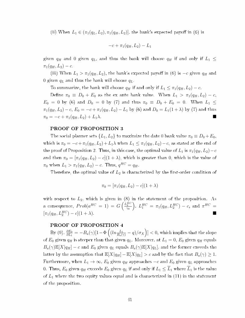
(ii) When L1 ∈ (π1(qL, L2), π1(qH , L2)], the bank's expected payo� in (6) is

−c+ π1(qH , L2)− L1

given qH and 0 given qL, and thus the bank will choose qH if and only if L1 ≤π1(qH , L2)− c.

(iii) When L1 > π1(qH , L2), the bank's expected payo� in (6) is −c given qH and

0 given qL and thus the bank will choose qL.

To summarize, the bank will choose qH if and only if L1 ≤ π1(qH , L2)− c.De�ne π0 ≡ D0 + E0 as the ex ante bank value. When L1 > π1(qH , L2) − c,

E0 = 0 by (6) and D0 = 0 by (7) and thus π0 ≡ D0 + E0 = 0. When L1 ≤π1(qH , L2)− c, E0 = −c+ π1(qH , L2)−L1 by (6) and D0 = L1(1 +λ) by (7) and thus

π0 = −c+ π1(qH , L2) + L1λ. �


The social planner sets {L1, L2} to maximize the date 0 bank value π0 ≡ D0 +E0,

which is π0 = −c+π1(qH , L2)+L1λ when L1 ≤ π1(qH , L2)− c, as stated at the end of

the proof of Proposition 2. Thus, in this case, the optimal value of L1 is π1(qH , L2)−cand then π0 = [π1(qH , L2) − c](1 + λ), which is greater than 0, which is the value of

π0 when L1 > π1(qH , L2)− c. Thus, qHC = qH .

Therefore, the optimal value of L2 is characterized by the �rst-order condition of

π0 = [π1(qH , L2)− c](1 + λ)

with respect to L2, which is given in (8) in the statement of the proposition. As

a consequence, Prob(aHC = 1) = G(LHC2

γ0

), LHC1 = π1(qH , L

HC2 ) − c, and πHC =

[π1(qH , LHC2 )− c](1 + λ). �


By (9), ∂E0

∂L1= −Ba(γ)[1−Φ

((ln L1

Ba(γ)− q)/σX

)] < 0, which implies that the slope

of E0 given qH is steeper than that given qL. Moreover, at L1 = 0, E0 given qH equals

Ba(γ)E[X|qH ]− c and E0 given qL equals Ba(γ)E[X|qL], and the former exceeds the

latter by the assumption that E[X|qH ]−E[X|qL] > c and by the fact that Ba(γ) ≥ 1.

Furthermore, when L1 →∞, E0 given qH approaches −c and E0 given qL approaches

0. Thus, E0 given qH exceeds E0 given qL if and only if L1 ≤ L1 where L1 is the value

of L1 where the two equity values equal and is characterized in (11) in the statement

of the proposition.

41

Thus, when L ≤ L1, the bank will choose qH , and its date 0 equity value will be

−c+

ˆ ∞L1

Ba(γ)

[XBa(γ)− L1] g(X; qH)dX

by (9) and its date 0 debt value will be

D0 =

ˆ ∞L1

Ba(γ)

L1(1 + λ)g(X; qH)dX

by (10), and therefore the date 0 bank value is

π0(L1, qH) = −c+

ˆ ∞L1

Ba(γ)

[XBa(γ) + L1λ] g(X; qH)dX.

Similarly, when L > L1, the bank will choose qL, and its date 0 equity value will

be´∞

L1Ba(γ)

[XBa(γ)− L1] g(X; qL)dX by (9) and its date 0 debt value will be

D0 =

ˆ ∞L1

Ba(γ)

L1(1 + λ)g(X; qL)dX

by (10), and therefore the date 0 bank value is

π0(L1, qL) =

ˆ ∞L1

Ba(γ)

[XBa(γ) + L1λ] g(X; qL)dX.

�


Recall from the proof of Proposition 4 that when L ≤ L1, the date 0 bank value is

π0(L1, qH) = −c+Ba(γ)A(

L1

Ba(γ), qH

)whereA

(L1

Ba(γ), q)≡´∞

L1Ba(γ)

[X + L1

Ba(γ)λ]g(X; q)dX.

Because ∂π0(L1,qH)∂Ba(γ)

= A − ∂A

∂( L1Ba(γ)

)L1

Ba(γ)> 0, the social planner will pick the value

of L2

X= γ to maximize Ba(γ). By (4), B0

(L2

X

)attains its maximal value at L2

X= γ0

and B1

(L1

X


X= γ1 where γ1 = eT−k where T is

characterized by h(T/σZ)/σZ = λ(1+λ)(1−α) . Thus, the social planner will set

L2

X= γ0

if B0(γ0) ≥ B1(γ1) and set L2

X= γ1 if B1(γ1) > B0(γ0).

42

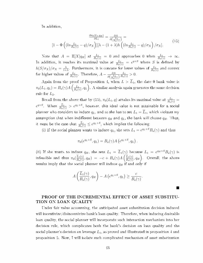
In addition,

∂π0(L1,qH)∂L1

= ∂A

∂( L1Ba(γ)

)=

[1− Φ(

(ln L1

Ba(γ)− q)/σX

)][λ− (1 + λ)h

((ln L1

Ba(γ)− q)/σX

)/σX ].

(15)

Note that A = E[X|qH ] at L1

Ba(γ)= 0 and approaches 0 when L1

Ba(γ)→ ∞.

In addition, it reaches its maximal value at L1

Ba(γ)= eq+S where S is de�ned by

h(S/σX)/σX = λ1+λ

. Furthermore, it is concave for lower values of L1

Ba(γ)and convex

for higher values of L1

Ba(γ). Therefore, A− ∂A

∂( L1Ba(γ)

)L1

Ba(γ)> 0.

Again from the proof of Proposition 4, when L > L1, the date 0 bank value is

π0(L1, qL) = Ba(γ)A(

L1

Ba(γ), qL

). A similar analysis again generates the same decision

rule for L2.

Recall from the above that by (15), π0(L1, q) attains its maximal value at L1

Ba(γ)=

eq+S. When L1

Ba(γ)> eqL+S, however, this ideal value is not attainable for a social

planner who considers to induce qL, and so she has to set L1 = L1, which violates my

assumption that when indi�erent between qH and qL, the bank will choose qH . Thus,

it must be the case that L1

Ba(γ)≤ eqL+S, which implies the following:

(i) If the social planner wants to induce qL, she sets L1 = eqL+SBa(γ) and thus

π0(eqL+S, qL) = Ba(γ)A

(eqL+S, qL

).

(ii) If she wants to induce qH , she sets L1 = L1(γ) because L1 = eqH+SBa(γ) is

infeasible and thus π0(L1(γ)Ba(γ)

, qH) = −c + Ba(γ)A(L1(γ)Ba(γ)

, qH

). Overall, the above

results imply that the social planner will induce qH if and only if

A

(L1(γ)

Ba(γ), qH

)− A

(eqL+S, qL

)≥ c

Ba(γ).

�

PROOF OF THE INCREMENTAL EFFECT OF ASSET SUBSTITU-

TION ON LOAN QUALITY

Under fair value accounting, the anticipated asset substitution decision induced

will incentivize/disincentivize bank's loan quality. Therefore, when inducing desirable

loan quality, the social planner will incorporate such interaction mechanism into her

decision rule, which complicates both the bank's decision on loan quality and the

social planner's decision on leverage L1, as proved and illustrated in proposition 4 and

proposition 5. Now, I will isolate such complicated mechanism of asset substitution

43

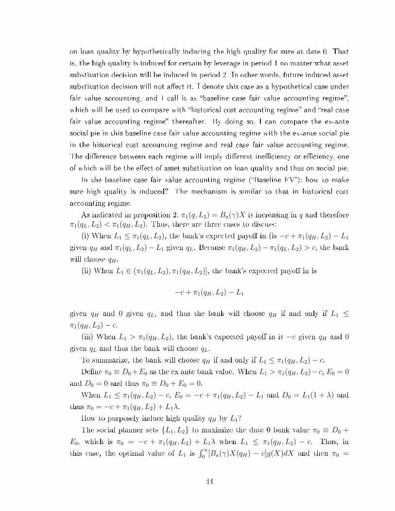
on loan quality by hypothetically inducing the high quality for sure at date 0. That

is, the high quality is induced for certain by leverage in period 1 no matter what asset

substitution decision will be induced in period 2. In other words, future induced asset

substitution decision will not a�ect it. I denote this case as a hypothetical case under

fair value accounting, and I call it as �baseline case fair value accounting regime�,

which will be used to compare with �historical cost accounting regime� and �real case

fair value accounting regime� thereafter. By doing so, I can compare the ex-ante

social pie in this baseline case fair value accounting regime with the ex-ante social pie

in the historical cost accounting regime and real case fair value accounting regime.

The di�erence between each regime will imply di�erent ine�ciency or e�ciency, one

of which will be the e�ect of asset substitution on loan quality and thus on social pie.

In the baseline case fair value accounting regime (�Baseline FV�): how to make

sure high quality is induced? The mechanism is similar to that in historical cost

accounting regime.

As indicated in proposition 2, π1(q, L2) = Ba(γ)X is increasing in q and thereforeπ1(qL, L2) < π1(qH , L2). Thus, there are three cases to discuss:

(i) When L1 ≤ π1(qL, L2), the bank's expected payo� in (is −c+ π1(qH , L2)− L1

given qH and π1(qL, L2)−L1 given qL. Because π1(qH , L2)− π1(qL, L2) > c, the bank

will choose qH .

(ii) When L1 ∈ (π1(qL, L2), π1(qH , L2)], the bank's expected payo� in is

−c+ π1(qH , L2)− L1

given qH and 0 given qL, and thus the bank will choose qH if and only if L1 ≤π1(qH , L2)− c.

(iii) When L1 > π1(qH , L2), the bank's expected payo� in is −c given qH and 0

given qL and thus the bank will choose qL.

To summarize, the bank will choose qH if and only if L1 ≤ π1(qH , L2)− c.De�ne π0 ≡ D0 +E0 as the ex ante bank value. When L1 > π1(qH , L2)−c, E0 = 0

and D0 = 0 and thus π0 ≡ D0 + E0 = 0.

When L1 ≤ π1(qH , L2) − c, E0 = −c + π1(qH , L2) − L1 and D0 = L1(1 + λ) and

thus π0 = −c+ π1(qH , L2) + L1λ.

How to purposely induce high quality qH by L1?

The social planner sets {L1, L2} to maximize the date 0 bank value π0 ≡ D0 +

E0, which is π0 = −c + π1(qH , L2) + L1λ when L1 ≤ π1(qH , L2) − c. Thus, in

this case, the optimal value of L1 is´ ∝0

[Ba(γ)X(qH) − c]g(X)dX and then π0 =

44

´ ∝0

[Ba(γ)X(qH) − c](1 + λ)g(X)dX, which is greater than 0, the value of π0 when

L1 >´ ∝0

[Ba(γ)X(qH)− c]g(X)dX. Thus, qHC = qH .

Therefore, the optimal value of L2 is characterized by the �rst-order condition of

π0(L1, qH) =

ˆ ∝0

[Ba(γ)X(qH)− c](1 + λ)g(X)dX.

Because ∂π0(L1,qH)∂Ba(γ)

=´ ∝0

(1 +λ)X(qH)g(X)dX > 0, the social planner will pick the

value of L2

X= γ to maximize Ba(γ). B0

(L2

X


X= γ0

and B1

(L1

X


X= γ1 where γ1 = eT−k where T is

characterized by h(T/σZ)/σZ = λ(1+λ)(1−α) . Thus, the social planner will set

L2

X= γ0

if B0(γ0) ≥ B1(γ1) and set L2

X= γ1 if B1(γ1) > B0(γ0).

Therefore, in the equilibrium, the social planner will choose optimal {L1, L2}tosurely induce qH and induce desirable asset substitution as following:

LFV−baseline1 =

´ ∝0

[Ba(γ)X(qH)− c]g(X)dX, LFV−baseline2 = γ0X if B0(γ0) ≥ B1(γ1)

and LFV−baseline2 = γ1X if B1(γ1) > B0(γ0)

Which induces the equilibrium bank decisions:

qFV−baseline = qH ;

aFV−baseline = 0 if B0(γ0) ≥ B1(γ1) and aFV−baseline = 1 if B1(γ1) > B0(γ0)

The equilibrium date 0 bank valueπFV−baseline0 =

´ ∝0

[Ba(γ)X(qH)−c](1+λ)g(X)dX.

Now, let's compare the ex-ante bank value under three regimes: Historical cost

accounting regime, Baseline Fair value accounting regime and Real Fair value ac-

counting regime.

HC: πHC0 = [π1(qH , L2)− c](1 + λ)

Baseline FV:πFV−baseline0 =

´ ∝0

[Ba(γ)X(qH)− c](1 + λ)g(X)dX

Real FV:πFV−real0 = −c+Ba(γ)A

(L1(γ)Ba(γ)

, qH

),

where A(L1(γ)Ba(γ)

, q)≡´∞L1(γ)Ba(γ)

[X + L1(γ)

Ba(γ)λ]g(X; q)dX.

Proof: πHC0 < πFV−baseline0 >? < π

FV−real0

π1(qH , L2) under HC is the weighted average π1for all possible Ba(γ), while under

base-lineBa(γ) is the max{B1(γ1), B0(γ0)}, so πFV−baseline0 > πHC0

LFV−baseline1 =

´ ∝0

[Ba(γ)X(qH)− c]g(X)dX

πFV−baseline0 =

´ ∝0

[X(qH)Ba(γ) + λL

FV−baseline1 − c

]g(X; qH)dX

πFV−real0 =

´∞LFV−Real1Ba(γ)

[X(q)Ba(γ) + λL

FV−Real1 − c

]g(X; q)dX =−c+Ba(γ)A

(LFV−Real1

Ba(γ), qH

)As proved in proposition 5,A

(LFV−Real1

Ba(γ), q

)is concave in L

FV−Real1 , while

45

πFV−baseline0 =

´ ∝0

[X(qH)Ba(γ) + λL


]g(X; qH)dX is increasing in

LFV−baseline1 ,but I assume that L

FV−baseline1 = π1(qH , L2)− c to induce qH for sure.

That is, at LFV−baseline1 , π

FV−baseline0 is maximized.

Now let's discuss the following cases:

Case I: LFV−Real1 = L

FV−baseline1

πFV−baseline0 =

´ ∝0

[X(qH)Ba(γ) + λL


]g(X; qH)dX

πFV−real0 |qH =


[X(qH)Ba(γ) + λL

FV−Real1 − c

]g(X; qH)dX

=´∞LFV−baseline1Ba(γ)

[X(qH)Ba(γ) + λL


]g(X; qH)dX

>´ ∝0

[X(qH)Ba(γ) + λL


]g(X; qH)dX = π

FV−baseline0

Case II: LFV−Real1 > L

FV−baseline1

πFV−real0 |qH =


[X(qH)Ba(γ) + λL

FV−Real1 − c

]g(XqH ; q)dX

>´∞LFV−baseline1Ba(γ)

[X(qH)Ba(γ) + λL


]g(X; qH)dX

>´ ∝0

[X(qH)Ba(γ) + λL


]g(X; qH)dX = π

FV−baseline0

Case III: LFV−Real1 < L

FV−baseline1

πFV−real0 |qL =


[X(qL)Ba(γ) + λL

FV−Real1 − c

]g(X; qL)dX

<´∞LFV−baseline1Ba(γ)

[X(qL)Ba(γ) + λL


]g(X; qL)dX

<´ ∝0

[X(qH)Ba(γ) + λL


]g(X; qH)dX = π

FV−baseline0

Therefore, I proved πFV−baseline0 > π

FV−real0 |qL or π

FV−baseline0 < π

FV−real0 |qH

�


Fair Value Accounting:

By (2), ∂γ0∂σZ

< 0. By (13), ∂B0(γ0)∂σZ

< 0. In contrast, by (14), ∂γ1∂σZ

> 0. By (13),∂B1(γ1)∂σZ

> 0. Therefore, B0(γ0) > B1(γ1) for lower values of σZ and vice versa.

Then, for lower values of σZ , the social planner will set L2 = γ0X to induce B0(γ0).

In these cases, a higher value of σZ will lead to a lower value of B0(γ0), which in turn

will lead to a lower value of L1(γ0) by (11). Furthermore, a lower value of L1(γ0) will

lead to a lower value of the left-hand side of (12), which implies that it will become

less bene�cial for the planner to induce qH .

By a similar reasoning, for higher values of σZ , the social planner will set L2 = γ1X

to induce B1(γ1). In these cases, a higher value of σZ will lead to a higher value of

B1(γ1), which in turn will lead to a higher value of L1(γ1) by (11). Furthermore, a

46

higher value of L1(γ1) will lead to a higher value of the left-hand side of (12), which

implies that it will become more bene�cial for the planner to induce qH .

The above results imply that when σZ is increasing from 0, LFV2 is decreasing �rst

(LFV2 = γ0X) and increasing later (LFV2 = γ1X). Such a pattern induces a = 0 �rst

and a = 1 later.

By Proposition 5, when σZ is increasing from 0, LFV1 is decreasing �rst (from

LFV1 = L1(γ0) to LFV1 = eqL+SB0(γ0)) and increasing later (from LFV1 = eqL+SB1(γ1)

to LFV1 = L1(γ1)). Such a pattern induces qH �rst, followed by qL, and eventually qH

later again.

By the above results and by Proposition 5, when σZ is increasing from 0, the

equilibrium date 0 bank value changes from πFV0 = B0(γ0)A(L1(γ0)B0(γ0)

, qH

)−c to πFV0 =

B0(γ0)A(eqL+S, qL

), then to πFV0 = B1(γ1)A

(eqL+S, qL

), and eventually to πFV0 =

B1(γ1)A(L1(γ1)B1(γ1)

, qH

)− c.

Historical Cost Accounting:

By (8),∂LHC2

∂σZ> 0. And because ∂γ0

∂σZ< 0, Prob(aHC = 1) = G

(LHC2

γ0

)is increasing

in σZ .

By (5),∂π1(LHC2 ,qH)

∂σZ> 0 and therefore

∂LHC1

∂σZ> 0 and

∂πHC0

∂σZ> 0.

Comparison of Fair Value Accounting and Historical Cost Accounting:

I �rst show that when σZ is su�ciently large, πFV0 > πHC0 .

Note that∂πHC0

∂σZ=´ LHC2

γ00 X

∂B1

(LHC2X

)∂σZ

g(X; qH)dX by the expression for πHC0 in

Proposition 3. Note that when σZ →∞, LHC2 →∞ and γ0 → 0, and thus

∂πHC0

∂σZ→ˆ ∞0

X∂B1

(LHC2

X

)∂σZ

g(X; qH)dX.

Next note that when σZ is su�ciently large, πFV0 = B1(γ1)A(L1(γ1)B1(γ1)

, qH

)− c

according to Proposition 5. Therefore,

∂πFV0

∂σZ= (1 + λ)

(L1(γ1)B1(γ1)

)2g(L1(γ1)B1(γ1)

)∂B1(γ1)∂σZ

+´∞L1(γ1)B1(γ1)

X ∂B1(γ1)∂σZ

g(X; qH)dX

+∂L1(γ1)∂σZ

[1−G

(L1(γ1)B1(γ1)

)] [λ− (1 + λ)h

((lnL1(γ1)

B1(γ1)− qH

)/σX

)/σX

].

(16)

47

Note that when σZ →∞, γ1 →∞ and B1 (γ1)→∞, and thus

∂πFV0

∂σZ→ (1 + λ)

(L1(γ1)B1(γ1)

)2g(L1(γ1)B1(γ1)

)∂B1(γ1)∂σZ

+´∞0X ∂B1(γ1)

∂σZg(X; qH)dX

+∂L1(γ1)∂σZ

[1−G

(L1(γ1)B1(γ1)

)] [λ− (1 + λ)h

((lnL1(γ1)

B1(γ1)− qH

)/σX

)/σX

].

(17)

Because the second and third terms of the preceding expression are both positive

and because its �rst term equals∂πHC0

∂σZin the limit, when σZ → ∞,

∂πFV0

∂σZ>

∂πHC0

∂σZ.

Because when σZ → ∞, both πFV0 and πHC0 go to ∞ and∂πFV0

∂σZ>

∂πHC0

∂σZ, it must be

the case that when σZ is su�ciently large, πFV0 > πHC0 .

Next I show that when σZ is su�ciently low, πFV0 > πHC0 where

πFV0 = B0(γ0)A

(L1(γ0)

B0(γ0), qH

)− c

according to Proposition 5.

Note that when σZ → 0, LHC2 → 0 and γ0 → 1, and thus π1 → E[X|qH ].

Thus, when σZ → 0, πHC0 → (1 + λ)E[X|qH ] − (1 + λ)c. Moreover, when σZ →0, γ0 → 1 and thus B0(γ0) → 1 + λ, which in turn implies that πFV0 → (1 +

λ)´∞L1(γ0)1+λ

[X + L1(γ0)

1+λλ]g(X; qH)dX − c. Because

´∞y

[X + yλ] g(X; qH)dX is increas-

ing in y for y < eqH+S, it must be the case that when σZ is su�ciently low, πFV0 > πHC0 .

Overall, because πFV0 is a U-shaped curve of σZ and πHC0 is an increasing function

of σZ , and because πFV0 > πHC0 for both extremely low values and extremely high

values of σZ , it must be the case that πHC0 > πFV0 for medium values of σZ and the

converse is true for extreme values of σZ .

The proof of the results regarding k follows the similar reasoning above and is

omitted. �



By (2), ∂γ0∂α

= 0. By (13), ∂B0(γ0)∂α

= 0. In contrast, by (14), ∂γ1∂α

> 0. By (13),∂B1(γ1)∂α

> 0. Therefore, B0(γ0) > B1(γ1) for lower values of α and vice versa.

Then, for lower values of α, the social planner will set L2 = γ0X to induce B0(γ0),

and for higher values of σZ , the social planner will set L2 = γ1X to induce B1(γ1).

In the latter case, a higher value of α will lead to a higher value of B1(γ1), which

in turn will lead to a higher value of L1(γ1) by (11). Furthermore, a higher value of

L1(γ1) will lead to a higher value of the left-hand side of (12), which implies that it

will become more bene�cial for the planner to induce qH .

48

The above results imply that when α is increasing from 0, LFV2 is constant �rst

(LFV2 = γ0X) and increasing later (LFV2 = γ1X). Such a pattern induces a = 0 �rst

and a = 1 later.

By Proposition 5, when α is increasing from 0, LFV1 is constant �rst (LFV1 =

eqL+SB0(γ0)) and increasing later (from LFV1 = eqL+SB1(γ1) to LFV1 = L1(γ1)). Such

a pattern induces qL �rst and qH later.

By the above results and by Proposition 5, when α is increasing from 0, the

equilibrium date 0 bank value changes from πFV0 = B0(γ0)A(eqL+S, qL

)to πFV0 =

B1(γ1)A(eqL+S, qL

), and eventually to πFV0 = B1(γ1)A

(L1(γ1)B1(γ1)

, qH

)− c.


By (8),∂LHC2

∂α> 0 and therefore Prob(aHC = 1) = G

(LHC2

γ0

)is increasing in α.


∂α> 0 and therefore

∂LHC1

∂α> 0 and

∂πHC0

∂α> 0.


I �rst show that when α is su�ciently large, πHC0 > πFV0 .

Note that when α = 1, B′1

(LHC2

X

)> 0 and thus LHC2 → ∞, which implies that

B1

(LHC2

X

)= E[Z](1+λ) and π1 = E[X|qH ]E[Z](1+λ). Thus, πHC0 = E[X|qH ]E[Z](1+

λ)2 − c(1 + λ).

Next note that when α = 1, πFV0 = B1(γ1)A(L1(γ1)B1(γ1)

, qH

)− c according to Propo-

sition 5. Because γ1 →∞ and B1 (γ1)→ E[Z](1 + λ) when α = 1,

πFV0 →ˆ ∞

L1(γ0)E[Z](1+λ)

[XE[Z](1 + λ) + L1(γ1)λ

]g(X; qH)dX − c.

By (11), πHC0 > πFV0 if and only if

E[X|qH ]E[Z](1 + λ)2 >´∞L1(γ0)

E[Z](1+λ)

XE[Z](1 + λ)2g(X; qH)dX − λE[Z](1 + λ)´∞

L1(γ0)E[Z](1+λ)

[X − L1(γ0)

E[Z](1+λ)

]g(X; qL)dX,

which always holds.

A similar reasoning demonstrates that when α is su�ciently low, πFV0 > πHC0 due

to (i) B0(γ0) > B1(γ1) and (ii) c is su�ciently high.

Overall, both πFV0 and πHC0 are increasing functions of α and in particular πHC0

is linear in α. In addition, because πFV0 > πHC0 when α = 0 and πHC0 > πFV0 when

α = 1, it must be the case that πHC0 > πFV0 for large values of α and vice versa. �



49

By Proposition 5, it is straightforward to show that πFV0 = Ba(γa)A(eqL+S, qL

)or πFV0 = Ba(γa)A

(L1(γa)Ba(γa)

, qH

)− c is increasing in σX .


For lognormal distributions, their density is decreasing in σX forX ∈ (eq−σX , eq+σX )

and is increasing in σX otherwise. Therefore,∂π1(LHC2 ,qH)

∂σX> 0 for lower values of σX

and∂π1(LHC2 ,qH)

∂σX< 0 for higher values of σX . Thus, π

HC0 follows the same pattern.


At σX = 0, πHC0 = πFV0 . Because πFV0 is increasing in σX and πHC0 is increasing

for lower values of σX and decreasing for higher values of σX , πHC0 > πFV0 for lower

values of σX and vice versa. �



A higher value of qH will lead to a higher value of the left-hand side of (12), which

implies that it will become more bene�cial for the planner to induce qH .

By Proposition 5, when qH is increasing from qL, LFV1 is constant �rst (LFV1 =

eqL+SBa(γa)) and increasing later (LFV1 = L1(γa)). Such a pattern induces qL �rst

and qH later.

By the above results and by Proposition 5, when qH is increasing from qL, the

equilibrium date 0 bank value is constant �rst (πFV0 = Ba(γa)A(eqL+S, qL

)) and

increasing later (πFV0 = Ba(γa)A(L1(γa)Ba(γa)

, qH

)− c).


By (8),∂LHC2

∂qH> 0 and therefore Prob(aHC = 1) = G

(LHC2

γ0

)is increasing in qH .


∂qH> 0 and therefore

∂LHC1

∂qH> 0 and

∂πHC0

∂qH> 0.


I �rst show that when qH is su�ciently large, πHC0 > πFV0 where

πFV0 = B1(γ1)A

(L1(γ1)

B1(γ1), qH

)− c



´∞L2γ0

XB0

(L2

X

)(1 + λ)g(X; qH)dX +

´ L2γ0

0 XB1

(L2

X

)(1 + λ)g(X; qH)dX >´∞

L1(γ1)B1(γ1)

XB1(γ1)(1 + λ)g(X; qH)dX − λB1(γ1)´∞L1(γ1)B1(γ1)

[X − L1(γ1)

B1(γ1)

]g(X; qL)dX.

(18)

50

The preceding inequality holds for su�ciently large values of qH , because as qH →∞,

LHC2 →∞ and L1(γa)→∞.

A similar reasoning demonstrates that when qH = qL, πFV0 > πHC0 .

Thus, it must be the case that πHC0 > πFV0 for large values of qH and vice versa.

The proof of the results regarding c follows the similar reasoning above and isomitted. �



By (13), B0(γ0) = 1 at λ = 0 and is linearly increasing in λ. By (13), B1(γ1) =

E[Z] < 1 at λ = 0 and is increasing and convex in λ. Therefore, B0(γ0) > B1(γ1) for

lower values of λ and vice versa.

Then, for lower values of λ, the social planner will set L2 = γ0X to induce B0(γ0),

and for higher values of λ, the social planner will set L2 = γ1X to induce B1(γ1). In

the latter case, a higher value of λ will lead to a lower value of the left-hand side of

(12), which implies that it will become less bene�cial for the planner to induce qH .

The above results imply that when λ is increasing from 0, the patterns of changes

in LFV2 , LFV1 , aFV , qFV , and πFV0 follow the same trend as what is described in

Proposition 6 for an increasing value of σZ .


By (8),∂LHC2

∂λ> 0 and therefore Prob(aHC = 1) = G

(LHC2

γ0

)is increasing in λ.


∂λ> 0 and therefore

∂LHC1

∂λ> 0 and

∂πHC0

∂λ> 0.


I �rst show that when λ is su�ciently large, πHC0 > πFV0 , where

πFV0 = B1(γ1)A

(L1(γ1)

B1(γ1), qH

)− c



´∞L2γ0

XB0

(L2

X

)(1 + λ)g(X; qH)dX +

´ L2γ0

0 XB1

(L2

X

)(1 + λ)g(X; qH)dX >´∞

L1(γ1)B1(γ1)

XB1(γ1)(1 + λ)g(X; qH)dX − λB1(γ1)´∞L1(γ1)B1(γ1)

[X − L1(γ1)

B1(γ1)

]g(X; qL)dX,

(19)

which holds for su�ciently large values of λ.

51

A similar reasoning demonstrates that when λ = 0,

πFV0 = πHC0 = E[X|qH ]− c

and∂πFV0

∂λ>

∂πHC0

∂λbecause qH is su�ciently high.

Overall, both πFV0 and πHC0 are increasing functions of λ. In addition, when λ = 0,

πFV0 = πHC0 and∂πFV0

∂λ>

∂πHC0

∂λ. Furthermore, when λ is su�ciently large, πHC0 > πFV0 .

Thus, it must be the case that πHC0 > πFV0 for large values of λ and vice versa. �

52

References

[1] Acharya, V., and S. Ryan 2016: Banks' Financial Reporting and Financial Sys-

tem Stability. Journal of Accounting Research: May 2016, Vol. 54, No. 2, pp.

277-340.

[2] Admati, A., and M Hellwig 2013. The Bankers' New Clothes: What's Wrong

With Banking and What to Do About It. Princeton University Press.

[3] Admati, A.; P. Demarzo; M. Hellwig; and P. P�eiderer. 2012. Debt Overhang

and Capital Regulation. Working paper, Stanford University.

[4] Allen, F. and E. Carletti 2008. Mark-to-Market Accounting and Liquidity Pric-

ing. Journal of Accounting and Economics 45(2-3), 358-378.

[5] Allen, F., E. Carletti, and R. Marquez 2011. Credit Market Competition and

Capital Regulation. Review of Financial Studies 24 (4): 983-1018.

[6] Bertomeu, J., L. Mahieux, and H. Sapra. 2018. Accounting versus Prudential

Regulation. Working paper, University of California at San Diego, Tillsburg Uni-

versity, and University of Chicago.

[7] Bleck, A., and P. Gao 2018. Mark-to-Market, Loan Retention, and Loan Origina-

tion. Working paper, University of British Columbia and University of Chicago.

[8] Bryant, J. 1980. A Model of Reserves, Bank Runs, and Deposit Insurance. Jour-

nal of Banking and Finance 4: 335-344.

[9] Bulow, J., J. Gold�eld, and P. Klemperer. 2013. Market-Based Bank Capital

Regulation. Working paper, Stanford University.

[10] Burkhardt, K., and R. Strausz 2009. Accounting Transparency and the Asset

Substitution Problem. The Accounting Review : May 2009 84 (3): 689-712.

[11] Calomiris, C. W. and C. M. Kahn 1991. The Role of Demandable Debt in Struc-

turing Optimal Banking Arrangements. American Economic Review 81: 497-513.

[12] Corona, C., L. Nan, and G. Zhang 2015. Accounting Information Quality, In-

terbank Competition, and Bank Risk-Taking. The Accounting Review 90 (3):

967-985.

53

[13] Corona, C., L. Nan, and G. Zhang 2019: Banks' Asset Reporting Frequency and

Capital Regulation: An Analysis of Discretionary Use of Fair-Value Accounting.

The Accounting Review 94(2): 157-178.

[14] Dang, T.; G. Gorton; B. Holmstöm; and G. Ordonez. 2014. Banks as Secret

Keepers. Working paper no. 14�022, Penn Institute for Economic Research.

[15] Dewatripont, M., and J. Tirole. 1993. E�cient Governance Structure: Impli-

cations for Banking Regulation, in Capital Markets and Financial Intermedia-

tion, edited by C. Mayer and X. Vives. Cambridge: Cambridge University Press:

12�35.

[16] Diamond, D., and P. Dybvig 1983. Bank Runs, Deposit Insurance, and Liquidity.

Journal of Political Economy 91 (3): 401-419.

[17] Gale, D. 2010. Capital Regulation and Risk Sharing. International Journal of

Central Banking : 187-204.

[18] Giammarino, R., T. Lewis, and D. Sappington 1993. An Incentive Approach to

Banking Regulation. Journal of Finance 48 (4): 1523�1542.

[19] Göx, R.F. and Wagenhofer, A., 2009. Optimal impairment rules. Journal of

Accounting and Economics, 48(1), pp.2-16.

[20] Gron, A., and A. Winton. 2001. Risk Overhang and the Market Behavior. Journal

of Business 74: 591�612.

[21] Heaton, J., D. Lucas, and R. McDonald 2010. Is Mark-to-Market Accounting

Destabilizing? Analysis and Implications for Policy. Journal of Monetary Eco-

nomics 57(10): 64�75.

[22] Holmstöm, B. 2015. Understanding the Role of Debt in the Financial System.

Working paper no. 479, Bank for International Settlements.

[23] Jensen, M., and W. Meckling. 1976. Theory of the Firm: Managerial Behav-

ior, Agency Costs, and Capital Structure. Journal of Financial Economics 4:

177�203.

[24] Kahn, C., and A. Winton 2004. Moral Hazard and Optimal Subsidiary Structure

for Financial Institutions. Journal of Finance 59: 2531�2576.

54

[25] Laux C., and C. Leuz 2009. The Crisis of Fair-value Accounting: Making Sense

of the Recent Debate. Accounting, Organizations and Society 34 (6): 826-834.

[26] Li, J. 2017. Accounting for Banks, Capital Regulation and Risk-Taking. Journal

of Banking and Finance 74 : 102-121.

[27] Lu, T., H. Sapra, and A. Subramanian 2019. Agency Con�icts, Bank Capital

Regulation, and Marking-to-Market. Working paper, University of Houston,

University of Chicago, and Georgia State University.

[28] Morgan, D. 2002. Rating Banks: Risk and Uncertainty in an Opaque Industry.

American Economic Review 92: 874�88.

[29] Myers, S. 1977. Determinants of Corporate Borrowing. Journal of Financial Eco-

nomics 5: 147�75.

[30] Nier, E., and U. Baumann. 2006. Market Discipline, Disclosure and Moral Hazard

in Banking. Journal of Financial Intermediation 15: 332�61.

[31] Plantin, G., H. Sapra, and H. Shin 2008. Marking-to-Market: Panacea or Pan-

dora's Box. Journal of Accounting Research 46 (2): 435�460.

[32] Subramanian, A. and B. Yang 2018. Dynamic Prudential Regulation. Working

paper, Georgia State University.

55

PRUDENTIAL REGULATION AND BANK ACCOUNTING

Documents

Transcript of PRUDENTIAL REGULATION AND BANK ACCOUNTING