Proyecto Fin de Carrera

Ingeniería Electrónica

Application of voting techniques to redundant

temperature measure of aircraft engines

Autor: Jesús Parrado Granado

Tutor: Mª Ángeles Martín Prats

Departamento de Ingeniería electrónica

Escuela Técnica Superior de Ingeniería

Universidad de Sevilla

Sevi lla, 2017

Proyecto Fin de Carrera Ingeniería de Electrónica (2ª Ciclo)

Application of voting techniques to redundant temperature measure of aircraft engines

Autor: Jesús Parrado Granado

Tutor: Mª Ángeles Martín Prats

Dep. de Ingeniería Electrónica

Escuela Técnica Superior de Ingeniería

Universidad de Sevilla

Sevilla, 2017

ABSTRACT 5

1 INTRODUCTION 1

1.1 A bit of history and current tendency in avionics 2 1.2 General concepts of avionics 4

2 FAULT-TOLERANCE TECHNIQUES 6

2.1 General concepts and definitions 6 2.2 Fault-tolerance strategies 6

2.2.1 Hardware redundancy 7 2.2.2 Software redundancy 10 2.2.3 Informational redundancy 10 2.2.4 Time redundancy 10

2.3 Voters and voting technics 11 2.4 Example of fault tolerance designs 12

2.4.1 SAPO (Samocinny Pocitac) 12 2.4.2 STAR (Self Testing and Repair) 12 2.4.3 General Purpose Computer (GPC) of space shuttle 13

3 FAULT-TOLERANCE IN AVIONICS 13

3.1 Redundant configurations 13 3.1.1 Quadruplex redundancy 13 3.1.2 Monitored triplex redundancy 14 3.1.3 Dissimilar redundancy 15

4 AIRCRAFT ENGINES 16

4.1 General concepts and operation 16 4.2 Measurement system of the engine 17 4.3 Measure of the internal temperature 18

5 VOTING TECHNIQUES USED 20

5.1 Inexact majority voting 21 5.2 Scored-based fuzzy voting algorithm with dynamic bandwidth 21

6 SYSTEM DESCRIPTION 22

6.1 Considerations 22 6.2 Inputs and outputs signals 22 6.3 How it works 23

7 SIMULATION MODEL 26

7.1 Model description 26 7.2 Simulations 27

8 CONCLUSIONS 36

9 FUTURE LINES 36

10 ANNEXES 38

9.1 References 38 9.2 List of abbreviations 38 9.3 Matlab function 40

ABSTRACT

The objective of the present document is to present a new configuration of a redundant system for aircrafts, with the final objective of improve its reliability. The system referred in the document is a special configuration of the temperature measures of the diverse internal stages of a turbofan engine. The model proposed can be used in others configurations of aircrafts engines.

In order to have a better understanding of the system, general concepts about avionics, turbofan engines and fault-tolerant are briefly described below, as well as real examples of real fault-tolerant systems. Inside the fault-tolerant systems, the concept of voter rule a very important role as moderator of different available inputs, for what it receive some importance throughout the document.

Finally, the simulation of several cases of faults over the proposed system are shown to put a test the model functionality.

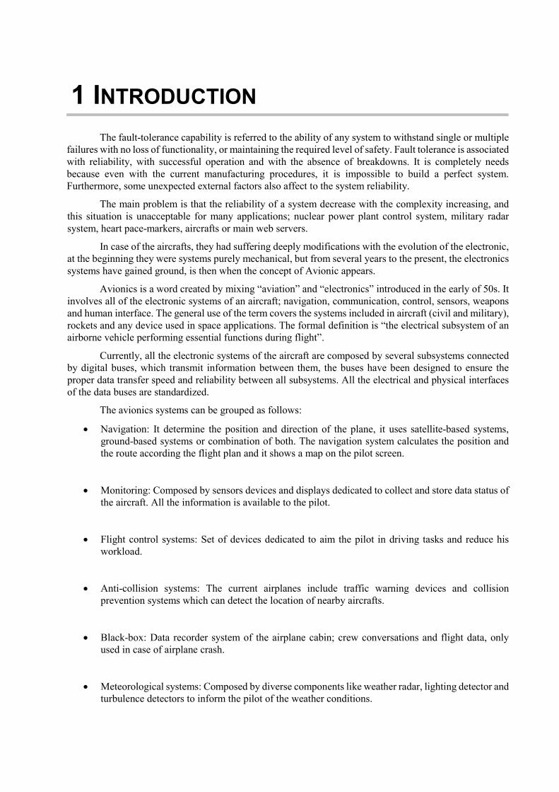
1 INTRODUCTION

The fault-tolerance capability is referred to the ability of any system to withstand single or multiple failures with no loss of functionality, or maintaining the required level of safety. Fault tolerance is associated with reliability, with successful operation and with the absence of breakdowns. It is completely needs because even with the current manufacturing procedures, it is impossible to build a perfect system. Furthermore, some unexpected external factors also affect to the system reliability.

The main problem is that the reliability of a system decrease with the complexity increasing, and this situation is unacceptable for many applications; nuclear power plant control system, military radar system, heart pace-markers, aircrafts or main web servers.

In case of the aircrafts, they had suffering deeply modifications with the evolution of the electronic, at the beginning they were systems purely mechanical, but from several years to the present, the electronics systems have gained ground, is then when the concept of Avionic appears.

Avionics is a word created by mixing “aviation” and “electronics” introduced in the early of 50s. It involves all of the electronic systems of an aircraft; navigation, communication, control, sensors, weapons and human interface. The general use of the term covers the systems included in aircraft (civil and military), rockets and any device used in space applications. The formal definition is “the electrical subsystem of an airborne vehicle performing essential functions during flight”.

Currently, all the electronic systems of the aircraft are composed by several subsystems connected by digital buses, which transmit information between them, the buses have been designed to ensure the proper data transfer speed and reliability between all subsystems. All the electrical and physical interfaces of the data buses are standardized.

The avionics systems can be grouped as follows:

Navigation: It determine the position and direction of the plane, it uses satellite-based systems, ground-based systems or combination of both. The navigation system calculates the position and the route according the flight plan and it shows a map on the pilot screen.

Monitoring: Composed by sensors devices and displays dedicated to collect and store data status of the aircraft. All the information is available to the pilot.

Flight control systems: Set of devices dedicated to aim the pilot in driving tasks and reduce his workload.

Anti-collision systems: The current airplanes include traffic warning devices and collision prevention systems which can detect the location of nearby aircrafts.

Black-box: Data recorder system of the airplane cabin; crew conversations and flight data, only used in case of airplane crash.

Meteorological systems: Composed by diverse components like weather radar, lighting detector and turbulence detectors to inform the pilot of the weather conditions.

Airplane management: Centralized control of the multiple systems like engines and room control of the aircraft.

Weapons and countermeasures system: only for military applications.

1.1 A bit of history and current tendency in avionics

The first plane was constructed by the Write brothers at early 20th century and it was entirely controlled by mechanical system and an internal combustion engine, it didn’t include any electrical system.

The first attempt to integrate electronic system onboard was in the 30s decade, with the introduction of diverse systems like; the radio, radar or single-axis autopilot.

The World War II provided a big stimulus for the development of the avionic systems; it involved the improvement of many systems like radar and autopilot. Nevertheless, almost all control devices of the airplanes still remained been mechanical. Moreover, it marked the beginning of the development of the first rockets.

The invention of the transistor and then the integrated circuit let to reduce the size of electronic devices and the improvement their capabilities. The new solid state devices are capable of performs arithmetical and logical operations that improve many electronic systems (fly computers, automatic pilot…).

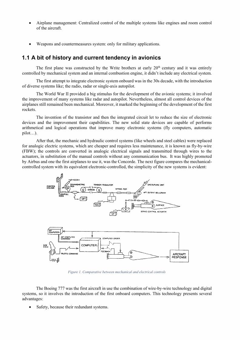
After that, the mechanic and hydraulic control systems (like wheels and steel cables) were replaced for analogic electric systems, which are cheaper and requires less maintenance, it is known as fly-by-wire (FBW); the controls are converted in analogic electrical signals and transmitted through wires to the actuators, in substitution of the manual controls without any communication bus. It was highly promoted by Airbus and one the first airplanes to use it, was the Concorde. The next figure compares the mechanical-controlled system with its equivalent electronic-controlled, the simplicity of the new systems is evident:

Figure 1. Comparative between mechanical and electrical controls

The Boeing 777 was the first aircraft in use the combination of wire-by-wire technology and digital systems, so it involves the introduction of the first onboard computers. This technology presents several advantages:

Safety, because their redundant systems.

Maneuverable, because the computers can command more adjustments than a pilot, this implies smoother movements of the airplane.

Efficient, because the electronic system are lighter and takes up less space than the mechanical and hydraulic systems. The solution requires less maintenance.

Because the low calculation power of the old computers, the airplanes were equipped with several computers to carry out the different tasks (for example, the Airbus A300 include 19 computers). With the improvement of the computers performance and the introduction of the digital systems, the number of onboard computers was decreasing while its computational capability was creasing (10 computers were included in the Airbus A310, 4 in the A320 and 2 in the A340 models).

This increasing of the number of software-controlled systems involves the introductions of new functionality:

For performance

o Flight management system

o Fuel management system

For improved safety

o Flight envelope protection

o Ground collision avoidance

For improve maintenance

o Aircraft condition monitoring

For improved passenger comfort

o Cabin environment control

Figure 2. Increasing of the electronic equipment onboard

In parallel, diverse communication bus protocols standard were defined and implemented in the commercial and military aircraft because the progressive need of higher speed of data transfer. The protocols are established by ARNIC (Aeronautical Radio Incorporated) for commercial airplanes and MIL for military.

In addition, the navigation systems other new subsystems were introduced; satellite communications, GPS…

Figure 3. On-board equipment set evolution, from analog to digital

New concept of systems were introduced mainly due to the evolution of the technologies, concept like IMA (Integrated Modular Avionics); a new integrated architecture of the on-board network composed by common hardware modules capable of support numerous applications. This concept replace multiple and separated processors with fewer and more centralized processing units, instead of the dedicated-application computers used until now. Other is the IVHM (Integrated Vehicle Health Management); the ability of a system to evaluate its state present and future based on the integration of systems that monitoring all aspects of the vehicle status to minimize the maintenance cost and the inactivity time.

Respect to the hardware design, the new concept of SOC (System On Chip) used in the new generation of portable devices like cell phones and tablets, has been recently introduced in the new designs.

1.2 General concepts of avionics

Due to the special application of the avionic systems, the required general specifications are critical. The next list includes the most common features of all systems/components used for avionic applications and the most common technics used in each case:

Reduced weight; SMD packages, Highly integrated chips (FPGA…), SOC systems, optimizing

component positioning, miniaturized connectors, thin cables for harness, thin/flexible board

material, communication over serial bus.

Low power consumption; CMOS technology, low voltage chipsets, reduced clock rate, Sleep

modes and enable inputs, optimize program execution.

In-flight reprogramming (only for space applications); capability to updates/verification software

during operation, EEPROM/flash memory as redundant boot device, programming protocol by

using telemetry.

Mechanical resilience; robust enclosure, encapsulated in resin, dampening connectors, shock

absorbing foam, locked connectors, perform crash test.

Functional redundancy; multiple identical subsystems, primary and alternate in parallel, triple

modular redundancy, diversity using different approaches (two equipment doing the same thing

with different programming languages, they must fail at the same moment).

Housekeeping & self-test: observation voltage and temperature, brownout detection, watchdog,

monitor radiation background.

Vacuum operation: (re)sublimating metals (Cd), avoid polymers containing plastifiers, avoid

fluoro-polymers (Teflon), use reactive adhesives (Epoxy), tape based on polyamide (kapton), test

outgassing in vacuum chamber.

Thermal management: model thermal budget of system, use ground planes and heat pipes to

distribute heart, use temperature control for sensitive components (battery packs), adjust emissivity

of surfaces to adjust thermal budget, thermal operation in vacuum chamber with sum simulator

The application of these features implies the additional needs in the aircraft, in order to maintenance its functionality:

Necessary to use AC and DC power generators onboard with more and more power. Currently it

uses AC generators and the DC voltage is obtained through rectifiers devices.

Additional protection systems like batteries, to ensure the uninterruptible power source and used

only in emergency cases.

The concept of avionics covers diverse functionality:

Data recorder:

o Acceleration

o Angular velocity

o Magnetic field vector

o Vehicle attitude from optical horizon

o Relative air velocity

o Ambient pressure

o Relative Humidity

o Local speed of sound

o Mechanical loads and vibrations

Housekeeping, functions:

o Self-test

o Subsystem monitoring

o Fault identification

o Power supply status

o Compartment pressure

o Board temperature

o Payload energy consumption

o Radiation dosage

Telemetry, functions:

o On-pad diagnostics

o Real-time flight data

o Remote control

o Radio beacon

Flight control, functions:

o Launch control

o Attitude

o Trajectory

o Mission abort

o Recovery

2 FAULT-TOLERANCE TECHNIQUES

2.1 General concepts and definitions

The most common technique to achieve fault-tolerance is the redundancy by the replication of multiple hardware components, additional data bit, or extra lines of program code verifying the results. It was pioneered by John von Neumann is 1950 in the work “Probabilistic logic and the synthesis of reliable organism from unreliable components”.

The basic element concepts are defined below:

Fault; any physical or logical defect, of any hardware or software component of a system.

Error; is the result of a fault from an informational point of view.

Failure; is an abnormal operation of a system caused by an error.

So the primary strategy of any system must be to avoid the propagation of the fault in order to prevent the error occurs, this implies the system should be the ability to detect and react in consequence.

2.2 Fault-tolerance strategies

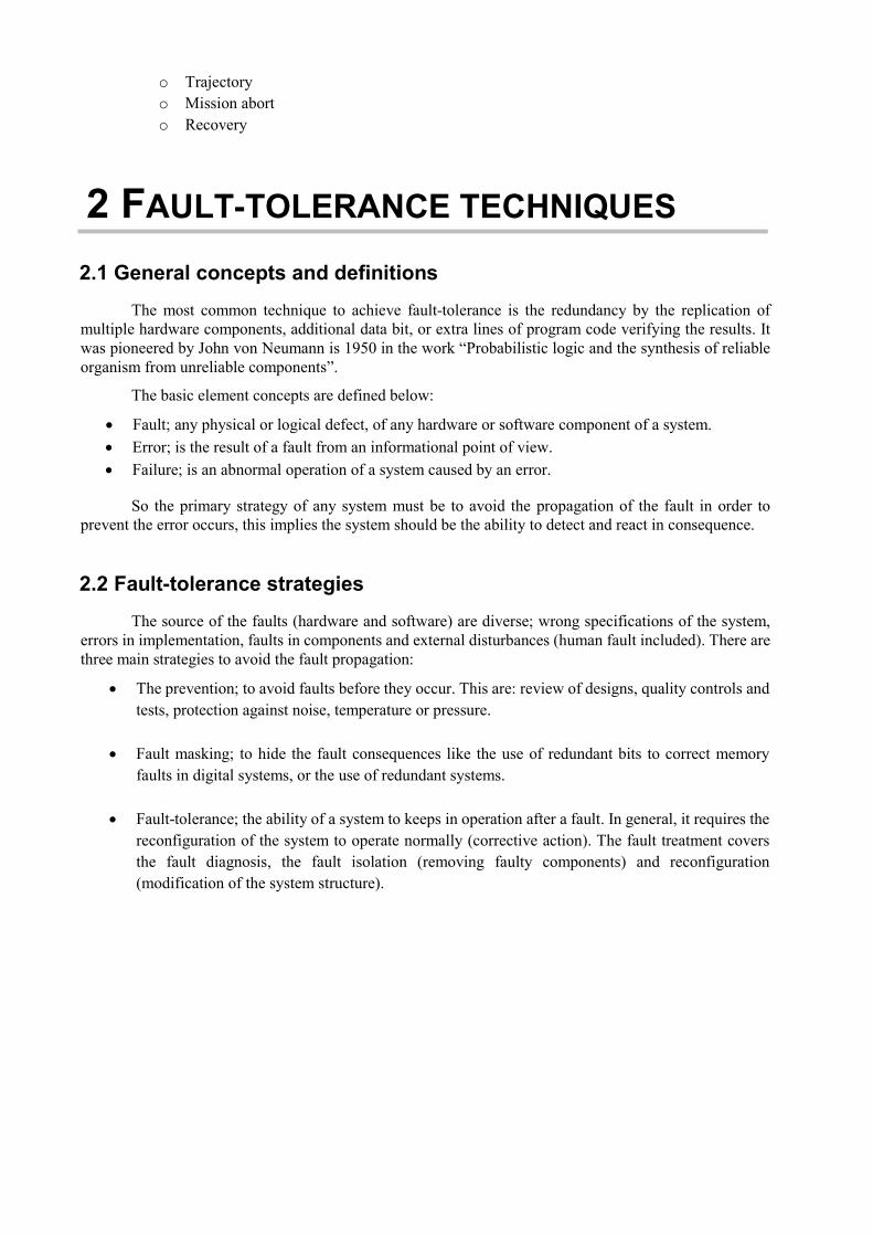
The source of the faults (hardware and software) are diverse; wrong specifications of the system, errors in implementation, faults in components and external disturbances (human fault included). There are three main strategies to avoid the fault propagation:

The prevention; to avoid faults before they occur. This are: review of designs, quality controls and

tests, protection against noise, temperature or pressure.

Fault masking; to hide the fault consequences like the use of redundant bits to correct memory

faults in digital systems, or the use of redundant systems.

Fault-tolerance; the ability of a system to keeps in operation after a fault. In general, it requires the

reconfiguration of the system to operate normally (corrective action). The fault treatment covers

the fault diagnosis, the fault isolation (removing faulty components) and reconfiguration

(modification of the system structure).

Wrong specifications

Errors in implementation

Fault in components

External disturbance

Software failures

Hardware failures

Errors System failures

0

FAULTPREVENTION

FAULT MASKING FAULT TOLERANCE

Figure 4. Barriers to avoid the fault propagation

Basically, the fault-tolerance ability of any system is achieved by redundancy, that is the multiplication of the physical elements of a system in a diverse way; hardware, software, temporal and informational. Neither of them are excluder themselves so they can be implemented into the same system.

Example: A digital system that read the measure of a sensor through an analogic-digital converter.

Hardware redundancy; the duplication of sensors, processor or A/D converters, compare the

signals and detect errors.

Software redundancy; software programmed to detect incorrect values of the sensor.

Temporal, if the sensor is jammed by an external interference the system must be able to read

the signal in different time interval to detect it (only applicable if the execution time is not

critical).

Informational, if the digital data transmission between the processor and A/D converter is

affected by noise, the digital word should include additional bits and error detection codes.

2.2.1 Hardware redundancy

The hardware redundancy is achieved by providing more than one physical instances of a hardware component. Sometimes, it is the only available method for the dependability of a system. Mainly there are two types:

Passive hardware redundancy: The passive technic is used to mask the failures and do not requires any external action. All the configurations achieves the masking of the failure.

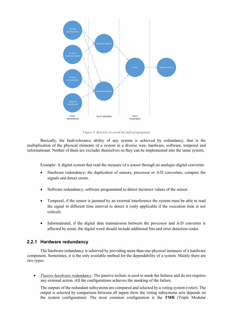
The outputs of the redundant subsystems are compared and selected by a voting system (voter). The output is selected by comparison between all inputs (how the voting subsystems acts depends on the system configuration). The most common configuration is the TMR (Triple Modular

Redundancy) although for a better performance it could be used the NMR (n-Modular Redundancy). The main disadvantage of the passive redundancy is that the system‘s output is always an unique result, so there is a subsystem without any redundancy configuration, in this case is the voter, but it is typically a very simple device compared to the redundant components and therefore its failure probability is much smaller.

MODULE 1

MODULE 2

MODULE 3

VOTERINPUT OUTPUT

Figure 5. Basic TMR configuration

There are multiple configurations of this topology, for example it’s possible to apply redundancy to the voting system to improve the reliability of the whole system by avoiding the single point of failure.

MODULE 1

MODULE 2

MODULE 3

VOTER 1

INPUT OUTPUTVOTER 2

VOTER 3

Figure 6. Improved TMR configuration

The voter can be achieved by hardware and software, the first one has better response in time. The most common example is the selection of the right value by the majority of the inputs.

Active hardware redundancy: The active technic requires an action to replace the damaged part, so the system is reconfigured, this may implies a temporally malfunction of the system while the new configuration is applied. The procedure has three phases; detection, location and recovery (sometimes the detection and location occurs at the same time), normally by comparison of the output of different subsystems. This technique is suitable for applications where temporary erroneous result is preferable to the high degree of redundancy required to achieve fault masking. The basic configuration is the duplication with comparison; the outputs of 2 identical modules are compared by a comparator, in case of disagreement a signal error is generated. After the detection of the fault, the system is not capable to take actions to return to the operational state.

MODULE 1

MODULE 2COMPARATOR

OUTPUT

ERRORINPUT

Figure 7. Duplication with comparation

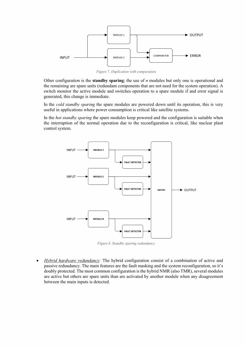
Other configuration is the standby sparing; the use of n modules but only one is operational and the remaining are spare units (redundant components that are not need for the system operation). A switch monitor the active module and switches operation to a spare module if and error signal is generated, this change is immediate.

In the cold standby sparing the spare modules are powered down until its operation, this is very useful in applications where power consumption is critical like satellite systems.

In the hot standby sparing the spare modules keep powered and the configuration is suitable when the interruption of the normal operation due to the reconfiguration is critical, like nuclear plant control system.

MODULE 1

FAULT DETECTOR

INPUT

MODULE 2

FAULT DETECTOR

MODULE N

FAULT DETECTOR

SWITCH OUTPUT

INPUT

INPUT

Figure 8. Standby sparing redundancy

Hybrid hardware redundancy: The hybrid configuration consist of a combination of active and passive redundancy. The main features are the fault masking and the system reconfiguration, so it’s doubly protected. The most common configuration is the hybrid NMR (also TMR), several modules are active but others are spare units than are activated by another module when any disagreement between the main inputs is detected.

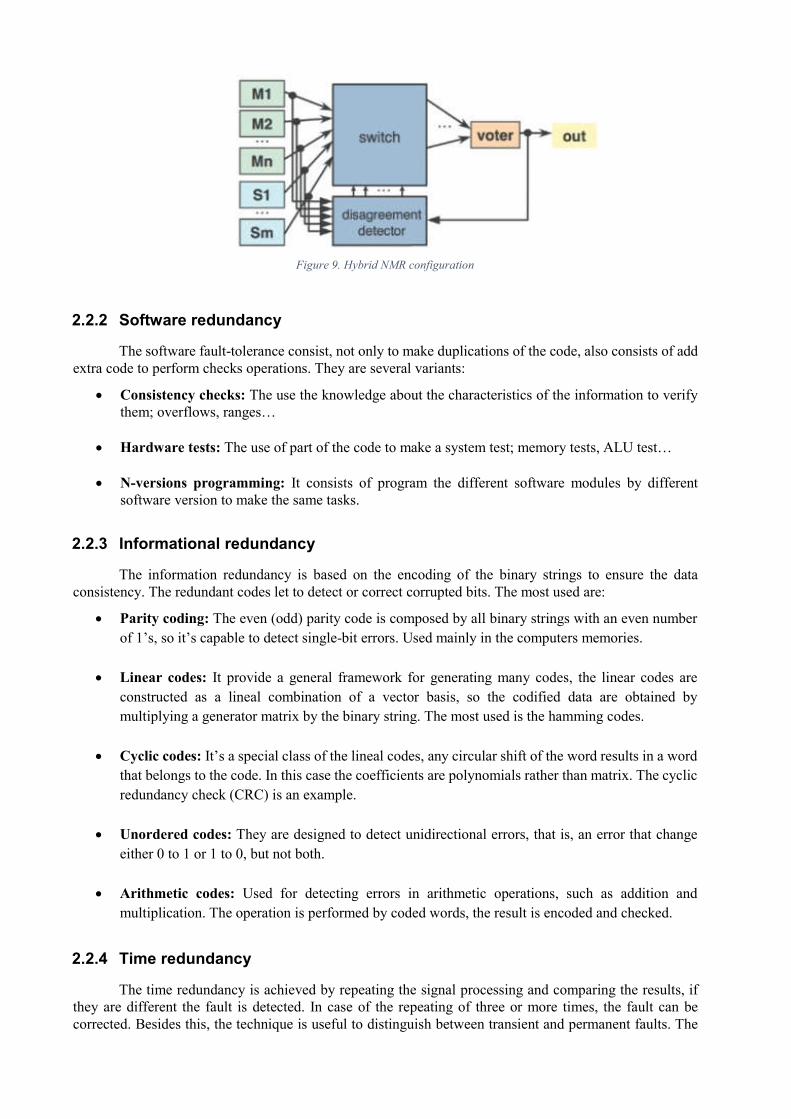
Figure 9. Hybrid NMR configuration

2.2.2 Software redundancy

The software fault-tolerance consist, not only to make duplications of the code, also consists of add extra code to perform checks operations. They are several variants:

Consistency checks: The use the knowledge about the characteristics of the information to verify them; overflows, ranges…

Hardware tests: The use of part of the code to make a system test; memory tests, ALU test…

N-versions programming: It consists of program the different software modules by different software version to make the same tasks.

2.2.3 Informational redundancy

The information redundancy is based on the encoding of the binary strings to ensure the data consistency. The redundant codes let to detect or correct corrupted bits. The most used are:

Parity coding: The even (odd) parity code is composed by all binary strings with an even number

of 1’s, so it’s capable to detect single-bit errors. Used mainly in the computers memories.

Linear codes: It provide a general framework for generating many codes, the linear codes are

constructed as a lineal combination of a vector basis, so the codified data are obtained by

multiplying a generator matrix by the binary string. The most used is the hamming codes.

Cyclic codes: It’s a special class of the lineal codes, any circular shift of the word results in a word

that belongs to the code. In this case the coefficients are polynomials rather than matrix. The cyclic

redundancy check (CRC) is an example.

Unordered codes: They are designed to detect unidirectional errors, that is, an error that change

either 0 to 1 or 1 to 0, but not both.

Arithmetic codes: Used for detecting errors in arithmetic operations, such as addition and

multiplication. The operation is performed by coded words, the result is encoded and checked.

2.2.4 Time redundancy

The time redundancy is achieved by repeating the signal processing and comparing the results, if they are different the fault is detected. In case of the repeating of three or more times, the fault can be corrected. Besides this, the technique is useful to distinguish between transient and permanent faults. The

main advantage is that it is no necessary to add extra hardware. Almost all the implementations are carried out in the design of the ALUs (Arithmetic Logic Unit) of the digital processors:

Alternative logic: Compares two data transmitted between a time interval, it’s capable of detect

faults in the bus lines.

Recompunting with shifted operands (RESO): The result of a computation of one system is

shifted to the left, after a time interval the operation is repeated and shifted to the right, both results

are compared.

Recomputing with swapped operands (RESWO): Both operands are splitted into two halves, the

first computation is performed as usual and the second one is performed with the lower and the

upper halves of operands swapped.

Recomputing with duplication with comparison (REDWC): It combines hardware redundancy

with time redundancy. An n-bit operation is performed by using n/2-bit devices twice. The operands

are splitted into two halves and the computations are performed separately, two operations for each

half.

2.3 Voters and voting technics

As it’s mentioned in previous section, the voter is the part of the system responsible for performing the selection of the output based on several criteria of selection for multiple and redundant inputs. Besides error masking, it has capabilities of noise removal.

In a general point of view and depending how it works, there are classified in two main groups:

A type (agreement-based); these produce an output whenever there is agreement between certain

number of inputs; plurality, majority. So, it doesn’t work in case of a total mismatching.

B type; the system generate an output based on a concrete rule; weighted average or mid-value, so

it always produces an output signal.

The operating rules are diverse and depends on the application; majority, plurality, weighted average, mid-value, score-based, maximum likelihood, step-wise negotiated. The main ones are:

The majority voter gives a result if there is agreement among most.

The mid-value voter calculates the mid-value of all inputs.

The weighted voter calculates the weighted mean of inputs.

Step-wise negotiated voting, the necessary information for calculations are taken from periodic self-

test of the system. Suitable for long-time space missions.

2.4 Example of fault tolerance designs

2.4.1 SAPO (Samocinny Pocitac)

SAPO means automatic computer, was the first Czechoslovak electromechanical computer and the first fault-tolerance computer ever built. It was operated from 1957 to 1960, and was designed with fault-tolerance technics thanks to its three arithmetic units (TMR configuration) operating in parallel (correct result was selected by voting) and the memory error detection system which automatically retries the data when an error is detected.

Figure 10. Image of SAPO computer

2.4.2 STAR (Self Testing and Repair)

It was designed in the 60’s and used in the Voyage probe for a 10 years mission to the outer planets. Various modules of the system were instruments to detect internal anomalies and signal faults conditions through special tests, and a repair processor effected the reconfiguration and performed the recovery. In addition, redundancy computers were checked each other by exchanging messages, and if one failure is detected its partner carried out the calculations. This technic was used in electronic systems of subsequences spacecraft.

Figure 11. General scheme of STAR system

Internal components of STAR:

Each module has triple redundancy.

5 processors TARP (Test and Repair Processor); 3 are continuously powered to determinate the

health of the others and 2 are inactive spares to replace faulty units.

2.4.3 General Purpose Computer (GPC) of space shuttle

The set is composed by five identical computers aboard. All the computers are IBM AP-101 (also used in the B-52 and B-1B bombers) descends from the System/360 IBM mainframe family of computers. Each one consists in a central processor and an I/O processor.

Four of the computers were arranged in a redundant configuration (by voting) and the fifth acts as backup unit programmed separately from the others, in addition a sixth spare unit is carried onboard to replace if necessary.

The four computers perform identical tasks from the same inputs and generating identical outputs through a common data bus. The computers managed the flight controllers, the crew display, monitoring systems and guidance, navigation and control functions.

The initial computer was upgraded to an improved version; the AP-101S (with hardware and software fully compatible with the previous version). This system includes additional protections like the memory; CMOS memory requires constant power, and cosmic rays can easily flip a bit. However, the memory has a fail-safe battery backup and an automatic error-correction circuit that constantly scans the memory for upsets and corrects errors. The MTBF was of 10000 hours.

3 FAULT-TOLERANCE IN AVIONICS

Actually, the probability of catastrophic failure of the flight control system must be less than 1 x 10-7 per hour for military aircraft and 1 x 10-9 per civil aircraft (a fleet of 3000 aircrafts flying 3000 hours per year would experience a failure in 100 years).

So the MTBF of a single system is about 3000 hours, in addition, the electronics systems has redundancy with multiple parallel devices and buses, so any system is able to tolerance at least two failures.

For another hand, the economic factor must be taken into account to design redundant systems, reaching an acceptable limit of the number of them according to the safety.

The main technics used in avionics design are the following:

3.1 Redundant configurations

The most clear example is the case of fly-by-wire (FBW) devices where the multiple redundancy is used, so each channel is independent from the others for critical components like actuators over control surfaces (flaps, ailerons …), including the power supply systems of the electronic and hydraulic system in order to avoid any weakness. The system must be designed to tolerate multiples failures, if one channel fails is overridden.

3.1.1 Quadruplex redundancy

The quadruple redundancy is used and the failures are detected by cross-comparison of the state of all channels, the majority voting of the result exclude the different, after that the failed channel is

disconnected, thus it is able to tolerate multiple failures. The voting algorithm selects the middle value of all sensors signals and compares with the others with it, if one of them differs more than a threshold, is considered like failure and the channel is disconnected (temporally or permanently).

Figure 12. Quadruplex redundancy

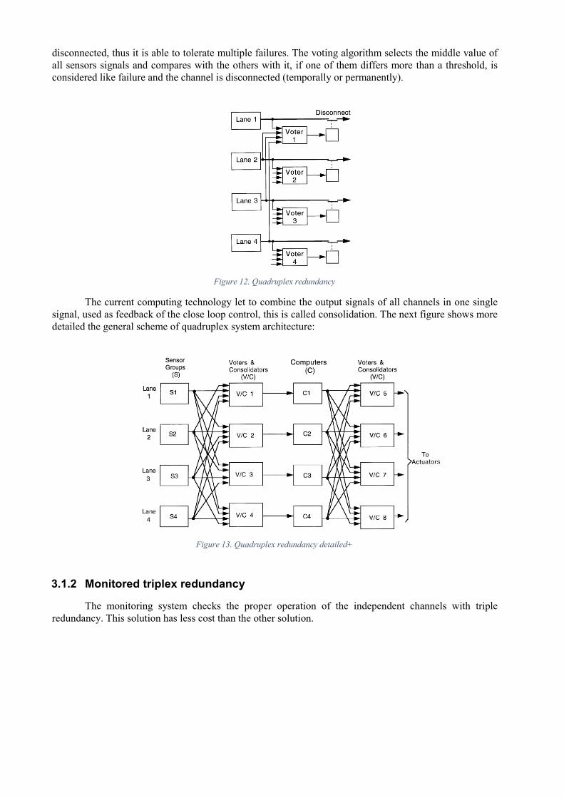
The current computing technology let to combine the output signals of all channels in one single signal, used as feedback of the close loop control, this is called consolidation. The next figure shows more detailed the general scheme of quadruplex system architecture:

Figure 13. Quadruplex redundancy detailed+

3.1.2 Monitored triplex redundancy

The monitoring system checks the proper operation of the independent channels with triple redundancy. This solution has less cost than the other solution.

Figure 14. Triplex redundancy

3.1.3 Dissimilar redundancy

The dissimilar redundancy consists of using different system with different configurations to make the same task, in short:

Use different type of microprocessors with different software.

Use of a back-up analogue system in addition to the digital system, the digital system is triplex or

quadruple level of redundancy.

Use of a back-up separate systems; sensors, computers, control…

The modern avionics control systems uses multiple control subsystems that control independent sections, so any individual failure is tolerated. Most of them are controlled by different actuators.

Figure 15. Airbus A380 flight control surfaces

The dissimilar system level is applicable both the hardware and the software, the computer control system includes another redundancy level; the primary computers (PRIM) and secondary computers (SEC) systems which are dissimilars.

4 AIRCRAFT ENGINES

4.1 General concepts and operation

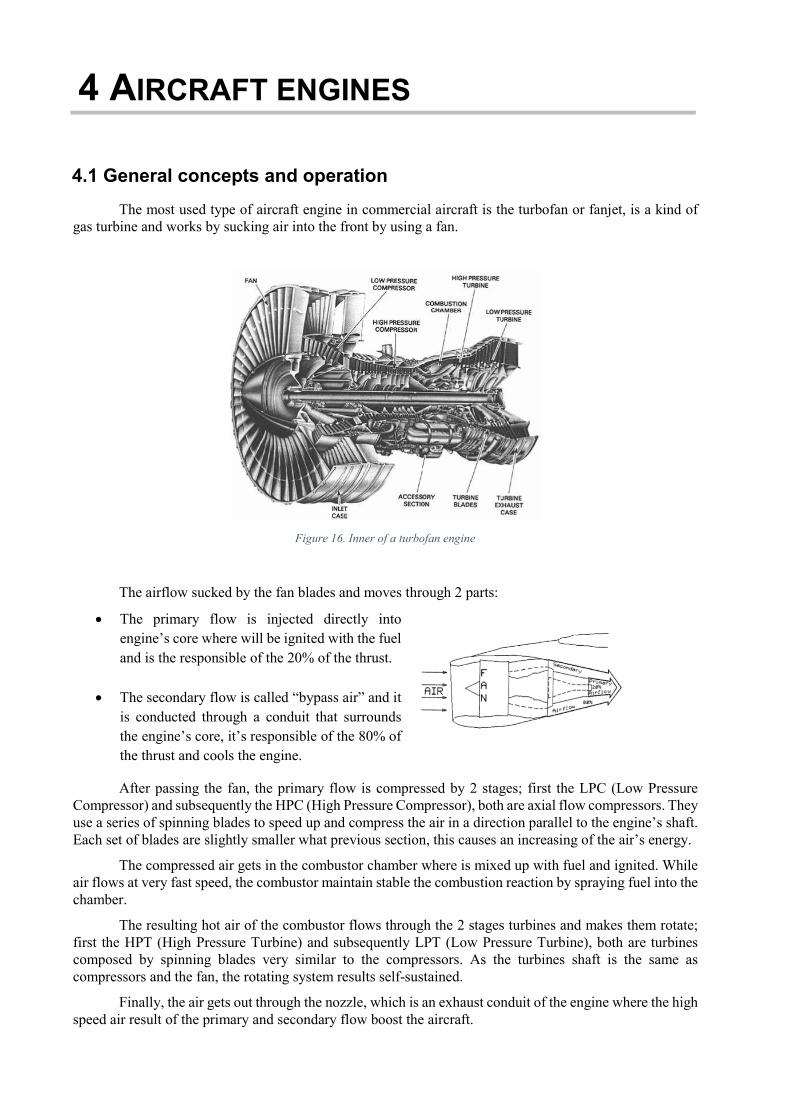
The most used type of aircraft engine in commercial aircraft is the turbofan or fanjet, is a kind of gas turbine and works by sucking air into the front by using a fan.

Figure 16. Inner of a turbofan engine

The airflow sucked by the fan blades and moves through 2 parts:

The primary flow is injected directly into

engine’s core where will be ignited with the fuel

and is the responsible of the 20% of the thrust.

The secondary flow is called “bypass air” and it

is conducted through a conduit that surrounds

the engine’s core, it’s responsible of the 80% of

the thrust and cools the engine.

After passing the fan, the primary flow is compressed by 2 stages; first the LPC (Low Pressure Compressor) and subsequently the HPC (High Pressure Compressor), both are axial flow compressors. They use a series of spinning blades to speed up and compress the air in a direction parallel to the engine’s shaft. Each set of blades are slightly smaller what previous section, this causes an increasing of the air’s energy.

The compressed air gets in the combustor chamber where is mixed up with fuel and ignited. While air flows at very fast speed, the combustor maintain stable the combustion reaction by spraying fuel into the chamber.

The resulting hot air of the combustor flows through the 2 stages turbines and makes them rotate; first the HPT (High Pressure Turbine) and subsequently LPT (Low Pressure Turbine), both are turbines composed by spinning blades very similar to the compressors. As the turbines shaft is the same as compressors and the fan, the rotating system results self-sustained.

Finally, the air gets out through the nozzle, which is an exhaust conduit of the engine where the high speed air result of the primary and secondary flow boost the aircraft.

Figure 17. Scheme of turbofan engine

The ratio between the mass of secondary and primary air flows is called as “bypass ratio”, and let to classify the engines into several categories:

High-bypass ratio (most used in civil aircrafts), gives a better consumption of fuel and less noise

engine.

Low-bypass ratio (most used in military aircrafts), gives a better response to a throttle changes,

small size and more efficiency at higher speed.

Zero-bypass ratio (used in specials military aircrafts), the engine is called turbojet and uses all the

air in combustion so gives more efficiency at very high speed.

Actually, all the engines are electronically controlled by a device called FADEC (Full Authority Digital Engine Control), it includes an internal computer ECU (Engine Control Unit) and electronic accessories to monitor and control the engine in order to operate at maximum efficiency. Among its features are; power management, flight deck indication, engine protection, engine starting, electronic valve control, feedback… Due to its criticality, the FADEC and ECU devices have redundant configuration in the aircraft.

4.2 Measurement system of the engine

The engine is a complex device that requires an appropriate control system to ensure a safety flight. Initially, the check of the general status of the aircraft was performed by the third cabinet crew, but after the evolution of the electronic systems this task was automated. Although the accessories of the engine may vary depending of the engine model, in a general point of view most used the instrumentation is the following:

EPR; Engine Pressure Ratio

EGT; Exhaust Gas Temperature

RPM; Revolutions Per Minute, this indicator may be simple or double depending on the number of

compressors (N1, N2) of the engine.

Power supply of the fuel control system

FF; Fuel Flow

Pressure of the fuel

Temperature of the fuel

Fuel flow counter

Control of oil for lubrication

Oil level

Vibration level of the engine

Temperature of turbine

4.3 Measure of the internal temperature

The temperature of the engine can be monitored in different locations; at the front, internal components and behind. The gas temperature is an operative limit of the engine, and it’s used to check the mechanical integration and to monitor the operating conditions.

The most important temperature measure is the input of the turbine, nevertheless is very difficult to measure in the most engines. For this, the measure of the turbine temperature at output stage is used as indicator of the temperature at input, despite they are different values. Normally, it’s used several thermocouples surrounding the exhaust gas duct perimeter, and the resulting measure is the mean of all thermocouples individually. For another hand, the measure of thermocouples in an individually way is also used.

The temperature of EGT in normally conditions is around 500-650 ºC for a high-bypass turbofan, for example the next diagram shows the evolution of different temperatures, pressures and velocity inside of General Electric J79:

Figure 18. Temperature curve of the engine

This graph is different for each type of engine and may vary in function the operating conditions and the design (presence of afterburner, manufacturing materials, cooling…).

The manufacturers have standardized reference planes within the gas path inside the engine called “stations”, that is, the engine has been divided into several zones with a concrete numerical value, so any sensor of temperature or pressure can be unequivocally located (see next figure); T5, T12, T25…

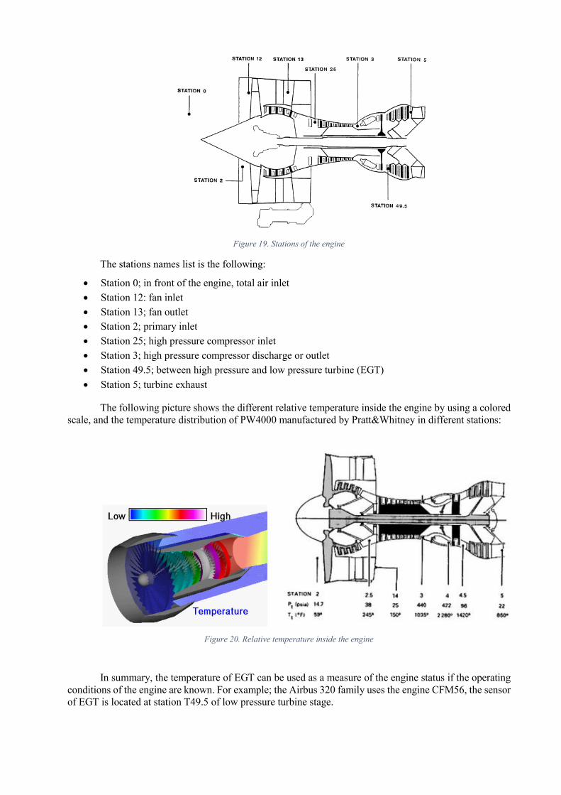
Figure 19. Stations of the engine

The stations names list is the following:

Station 0; in front of the engine, total air inlet

Station 12: fan inlet

Station 13; fan outlet

Station 2; primary inlet

Station 25; high pressure compressor inlet

Station 3; high pressure compressor discharge or outlet

Station 49.5; between high pressure and low pressure turbine (EGT)

Station 5; turbine exhaust

The following picture shows the different relative temperature inside the engine by using a colored scale, and the temperature distribution of PW4000 manufactured by Pratt&Whitney in different stations:

Figure 20. Relative temperature inside the engine

In summary, the temperature of EGT can be used as a measure of the engine status if the operating conditions of the engine are known. For example; the Airbus 320 family uses the engine CFM56, the sensor of EGT is located at station T49.5 of low pressure turbine stage.

Figure 21. EGT thermocouple harness and probes of CFM59 engine

It’s composed by 9 thermocouple probes (chromel/alumel) connected into a junction box, the temperature is sensed and averaged.

Figure 22. Wiring diagram of the EGT thermocouplers

Due to its high redundant configuration, it’s considered a very high reliable measure.

5 VOTING TECHNIQUES USED

5.1 Inexact majority voting

The inexact voting is one of the most used technique in critical systems. The meaning of the inexactitude consists of that the inputs are not exactly the same but the different between them is smaller than a determined threshold. This threshold must be carefully chosen because can lead to calculate a wrong result.

Given N inputs, if at least (� 1) 2⁄ elements outcomes in the decided majority group, that is, they

meet the expression ��� ��� = ��� < ������, with � ≠ � and where ��� the distance between results and

umbral is the voter threshold. Then the output is selected as the input with lowest range with all components of the subgroup. This means, the result is calculated by comparing all the couples of inputs and selecting those with lower range.

If is not possible to select a majority group then the technique is not applicable (that means that there is no (� 1) 2⁄ elements in any majority group). In this case, the system uses the scored-based fuzzy voting algorithm, in order to provide the best possible result.

5.2 Scored-based fuzzy voting algorithm with dynamic bandwidth

When system information is low, the fuzzy voting approach give better results than inexact majority option. To each module signal output a score is calculated as a function of the distance (���) between the

modules and normalized respect to the maximum values in order to calculate the fuzzy membership function.

For another hand, a dynamic bandwidth is used based on statistical method parameters to avoid the main disadvantage of the static bandwidth; it works only for a concrete set of data within a range.

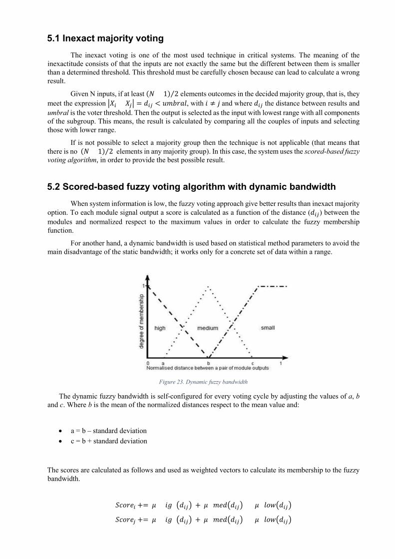
Figure 23. Dynamic fuzzy bandwidth

The dynamic fuzzy bandwidth is self-configured for every voting cycle by adjusting the values of a, b and c. Where b is the mean of the normalized distances respect to the mean value and:

a = b – standard deviation

c = b + standard deviation

The scores are calculated as follows and used as weighted vectors to calculate its membership to the fuzzy bandwidth.

������ += � �� ����� + � �������� � ��������

������ += � �� ����� + � �������� � ��������

The output of the voter depends so the score magnitude:

If ∑ ������ > 0 then ������ =∑ ������ ��

∑ �������

Otherwise ������ =∑ ��

��

��

6 SYSTEM DESCRIPTION

6.1 Considerations

Before start the description of how the system works, it’s necessary to list a brief list of considerations had been taken into account:

The temperature of any intermediate stage of an engine can be approximated, in a non-accurate

way, from the magnitude of EGT.

The measure of EGT is considered a very reliable system due to its special redundant configuration.

The temperature measure of any other stage is less reliable than EGT, because have less redundancy.

For the temperature measure of an intermediate stage of the engine, it’s considered a triple

redundant system (TMR), nevertheless it’s expandable to N-redundant systems.

All thresholds must be adjusted by the engine manufacturer.

6.2 Inputs and outputs signals

The inputs of the system are listed below:

Temperature measures of the intermediate stage of the engine (T12, T25…), really it doesn’t matter

which one. It’s considered a TMR configuration for each one and named generically like “Temp.

1”, “Temp. 2” and “Temp. 3”, or T1, T2 and T3.

Temperature measure of the EGT stage (Exhaust Gas Temperature). It’s considered as the most

reliable measure due to its 9-parallel sensors configuration; “Temp EGT”.

The outputs are the following:

The resulting temperature measure of the algorithm, it could be directly any of the inputs measures

or a calculation from them, is labeled as “OUTPUT” or “Xo”.

“Warning” signal, it actives if it’s possible to calculate an output but any (not all) of the measures

“Temp. i” are out of the reliable threshold.

“Error” signal, it actives if all measures of the TMR configuration are out of the reliable threshold.

In addition, the following variables are also considered:

Threshold surrounded the reliable measure. All measures inside this area have similar magnitude to

EGT value; “umbral EGT” or “umbral”. This is considered the security threshold.

Threshold surrounded the measures of TMR system “umbral medidas” or “umbral2” all measures

inside this area have similar magnitude, but not necessarily are similar to EGT value.

6.3 How it works

The simplified scheme of the algorithm is the following:

Normalization if scorei<0

Normalization respecto to maximum value

ndij = dij/max(dij)

How manydi-aux<=umbral?

Distance calculationdi-aux/dij

Input: Mi, Maux, umbral

Warning =1Xo = Mi

Warning =1Xo = (Mi+Mj)/2 dii<=umbral2?

Error =1

No

cdn

cdncb

dnb

bdnccb

cdn

bdnaab

adn

adnab

dnb

adn

cdn

cdncb

dnb

bdnccb

cdn

bdnaab

adn

adnab

dnb

adn

ij

ijij

ijij

ijij

ijij

ij

ij

ijij

ijij

ijij

ijij

ij

1

1

j

1

1

i

scorescore

scorescore

j

i

Inexact majority voting:Xo=menor(dij)

Yes

scorei>0?

Xo=∑scorei*Mi /∑scoreiXo=∑Mi /n

SI

NO

Bandwidth calculation; a, b, c

1 2 0 3

Output: Xo, warning, error

Figure 24. Simplified scheme of the algorithm

It’s divided into several parts:

1. Calculation of 2 sets of distances:

a. Between the different inputs “Ti” of the TMR system, “dij”. (where i and j are 1, 2 and 3)

b. Between each input “Ti” of the TMR system and EGT measure, “di-aux”

2. Depending on the number of distances “di-aux” that are within threshold with EGT measure (“umbral”) take different path:

Case 1. There is an unique input “Ti” inside the threshold, so “Ti” is the selected output “Xo”

but the “Warning” signal is enabled because there is some kind of problem (too many inputs

out of the security threshold).

Case 2. There are 2 measures inside the threshold (“umbral”), the output is calculated from the

mean value between them. The “Warning” signal is also enabled (one input is out of the security

threshold).

Case 3. All measures are inside the security threshold, so all are considered as valid. To

calculate the output “Xo” a new comparison is made with a new threshold, but only using the

measures of the engine’s intermediate stage; “umbral2”. Depending on the result of this new

comparison, the system calculate the final output by inexact majority voting or fuzzy weighted-

average voting based on score with variable bandwidth.

The scores are calculates as piecewise-defined function depending of the magnitudes a, b and c.

cdn

cdncb

dnb

bdnccb

cdn

bdnaab

adn

adnab

dnb

adn

cdn

cdncb

dnb

bdnccb

cdn

bdnaab

adn

adnab

dnb

adn

ij

ijij

ijij

ijij

ijij

ij

ij

ijij

ijij

ijij

ijij

ij

1

1

j

1

1

i

scorescore

scorescore

j

i

Finally, the output outcomes depending of the score magnitude as explained in the previous section. No signals of “Error” or “Warning” is activated in this case.

Case 0. This case considers that all measures are out of the reliable threshold, so the “Error”

signal is enabled. For the calculation of the optimal output, operates as the same way than Case

3.

The main advantage of this process, the system always provide the best output as possible, even when exists total disagreement between all inputs. Below is the complete disaggregated scheme:

d1-aux<=umbral

Aux=Medida1

SI

Contador ++

d2-aux<=umbral

Aux=Aux +Medida2

SI

Contador ++

NO

d3-aux<=umbral

Aux=Aux+Medida3

SI

Contador ++

NO

NO

Contador?

Error=1

0

Warning = 1 Warning = 1

1 2 3

Xo = Aux Xo = Aux/2

Calculo distancias:di-aux=│Mi-Maux│

dij=│Mi-Mj│

dij<=umbral2

Menor=d12

d12>d13

Menor=d13

SI

SI

d12>d23

Xo=M3

SI

Xo=M1

NO

d13>d23

Menor=d23

SI

Xo=M2

NO

d12>d23

NO

Menor=d23

SI

d23>d13

Xo=M2 Xo=M1

SI

NO

Xo=M1

NO

Xo=M2

NO

Normalización distancias:dn12 = d12/max(dij)dn13 = d13/max(dij)dn23 = d23/max(dij)

Calculo ancho de banda: b = valor medio(ndij)

a=desviación_estandar(ndij)-bc=desviación_estandar(ndij)+b

scorei<0

cdn

cdncb

dnb

bdnccb

cdn

bdnaab

adn

adnab

dnb

adn

cdn

cdncb

dnb

bdnccb

cdn

bdnaab

adn

adnab

dnb

adn

ij

ijij

ijij

ijij

ijij

ij

ij

ijij

ijij

ijij

ijij

ij

1

1

j

1

1

i

scorescore

scorescore

j

i

Normalización:score1n = score1 - min(scorei)score2n = score2 - min(scorei)score3n = score3 - min(scorei)

Si

NO

scorein>0

Xo=∑scorei*Mi /∑scoreiXo=∑Mi /n

SI

NO

VOTO MAYORIA INEXACTAVOTO DIFUSO BASADO EN PESO PROMEDIO

PONDERADO CON ANCHO DE BANDA DINÁMICO

Medida 1 (M1)Medida 2 (M2)Medida 3 (M3)

Medida fiable (Maux)

umbral umbral2

Salida:Xo

ErrorWarning

Xo=0Error=0

Warining=0

Coincidencias de medidas dentro de umbral fiable:1 La salida es la medida directa2 La salida es la media de las dos3 Cálculo por voto

0 Cálculo por voto pero con señal de error

Figure 25. Complete scheme of the algorithm

7 SIMULATION MODEL

7.1 Model description

The simulation software used is Matlab Simulink, the main core of the simulation is the algorithm that has been programmed by using an embedded Matlab function.

Figure 26. Simulation model

The inputs are located at left side:

Temperatures of TMR system, and of EGT.

Both threshold labeled as “umbral_1” (only for TMR measures) and “umbral_2” (for EGT

measure).

“aux_in_x” are the values of the scores calculated by the algorithm, the input feedback signals

(calculated by scored-based fuzzy voting algorithm).

The outputs are located at right side:

The output of the system, it is the calculated temperature.

Warning signal, it’s enabled when the system estimate that the calculations are correct but one of

the inputs is wrong.

Error signal, it’s enabled when more than one input is wrong, so the result cannot be considered

reliable.

Debug, used only for code depuration.

“aux_out_x” values of the scores calculated by the algorithm, the output feedback signals

(calculated by scored-based fuzzy voting algorithm).

7.2 Simulations

Some representative cases are presented in this section, because it’s impossible to cover all possibilities. In some cases, the inputs are constants values, so the representation of the Simulink model is shown. All values of inputs and outputs represent Celsius degree.

CASE 1. Normal operation, the system gives the result the measure most closed to EGT value.

INPUTS:

EGT = 420

Umbral EGT = 50

Umbral medidas = 20

T1 = 405

T2 = 400

T3 = 395

b. RESULTS:

Output = 405

Warning = 0

Error = 0

CASE 2. One measure damaged so it’s out of range. The system gives the right result but enables

the warning signal.

INPUTS:

EGT = 420

Umbral EGT = 50

Umbral medidas = 20

T1 = 800

T2 = 400

T3 = 395

RESULTS:

Output = 397.5

Warning = 1

Error = 0

CASE 3. Only one measure is close to EGT value. The system gives the right result but enables the

warning signal, because 2 measures of TMR are out of security threshold.

INPUTS

EGT = 420

Umbral EGT = 50

Umbral medidas = 20

T1 = 800

T2 = 800

T3 = 395

RESULTS:

Output = 395

Warning = 1

Error = 0

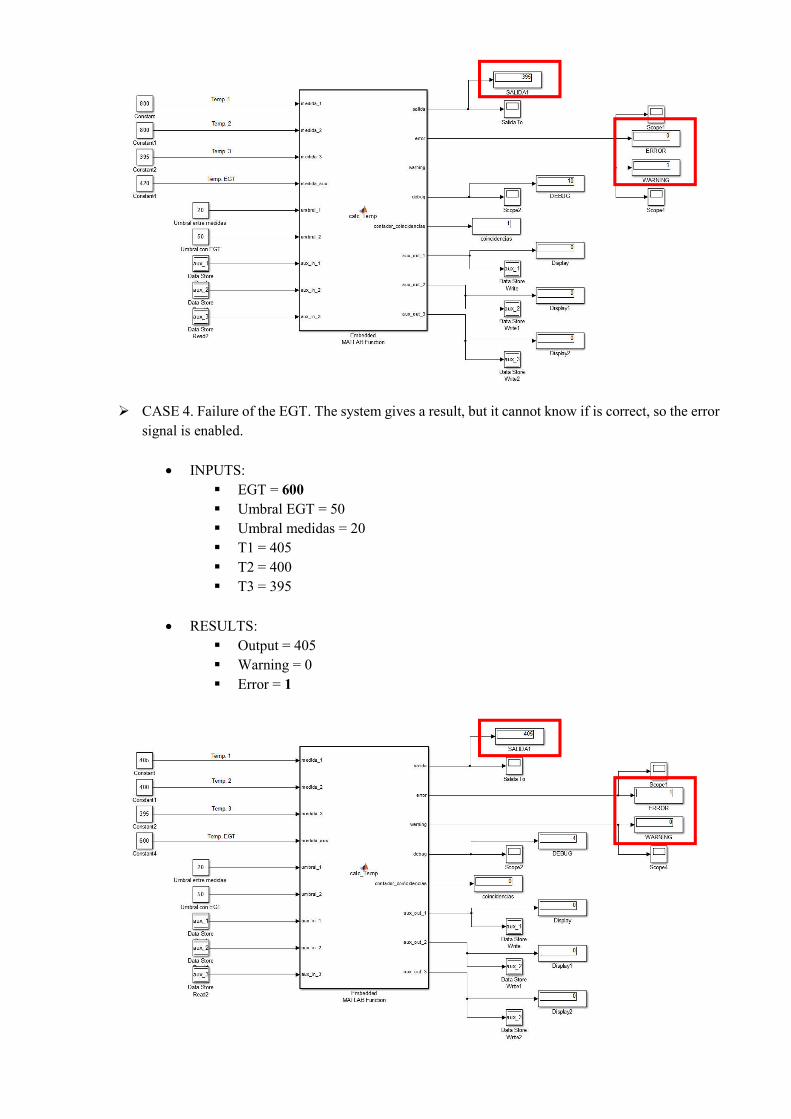
CASE 4. Failure of the EGT. The system gives a result, but it cannot know if is correct, so the error

signal is enabled.

INPUTS:

EGT = 600

Umbral EGT = 50

Umbral medidas = 20

T1 = 405

T2 = 400

T3 = 395

RESULTS:

Output = 405

Warning = 0

Error = 1

CASE 5. Failure of the EGT and one measure. The systems uses 2 measures of TMR to calculate

the output, but it cannot know if is correct (error enabled).

INPUTS

EGT = 600

Umbral con EGT = 50

Umbral entre medidas = 20

T1 = 10

T2 = 400

T3 = 395

RESULTS:

Output = 400

Warning = 0

Error = 1

CASE 6. One measure affected by high random noise. The system gives a correct result with very

small variations (less than 3 degrees) in comparison with the noise source.

INPUTS:

EGT = 420

Umbral con EGT = 50

Umbral entre medidas = 20

T1 = see figure

T2 = 400

T3 = 395

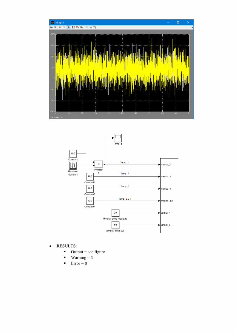
RESULTS:

Output = see figure

Warning = 1

Error = 0

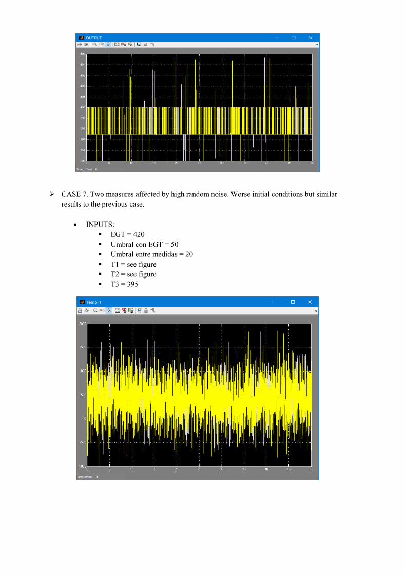
CASE 7. Two measures affected by high random noise. Worse initial conditions but similar

results to the previous case.

INPUTS:

EGT = 420

Umbral con EGT = 50

Umbral entre medidas = 20

T1 = see figure

T2 = see figure

T3 = 395

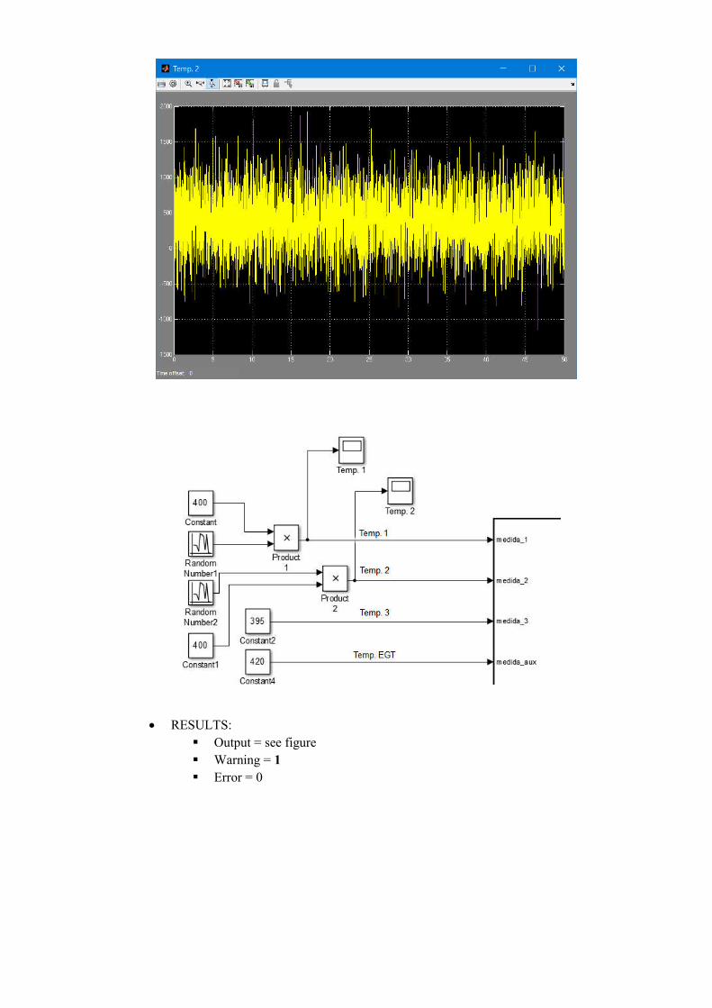
RESULTS:

Output = see figure

Warning = 1

Error = 0

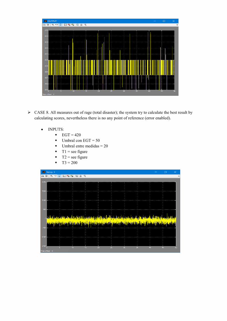
CASE 8. All measures out of rage (total disaster); the system try to calculate the best result by

calculating scores, nevertheless there is no any point of reference (error enabled).

INPUTS:

EGT = 420

Umbral con EGT = 50

Umbral entre medidas = 20

T1 = see figure

T2 = see figure

T3 = 200

RESULTS:

Output = see figure

Warning = 0

Error = 1

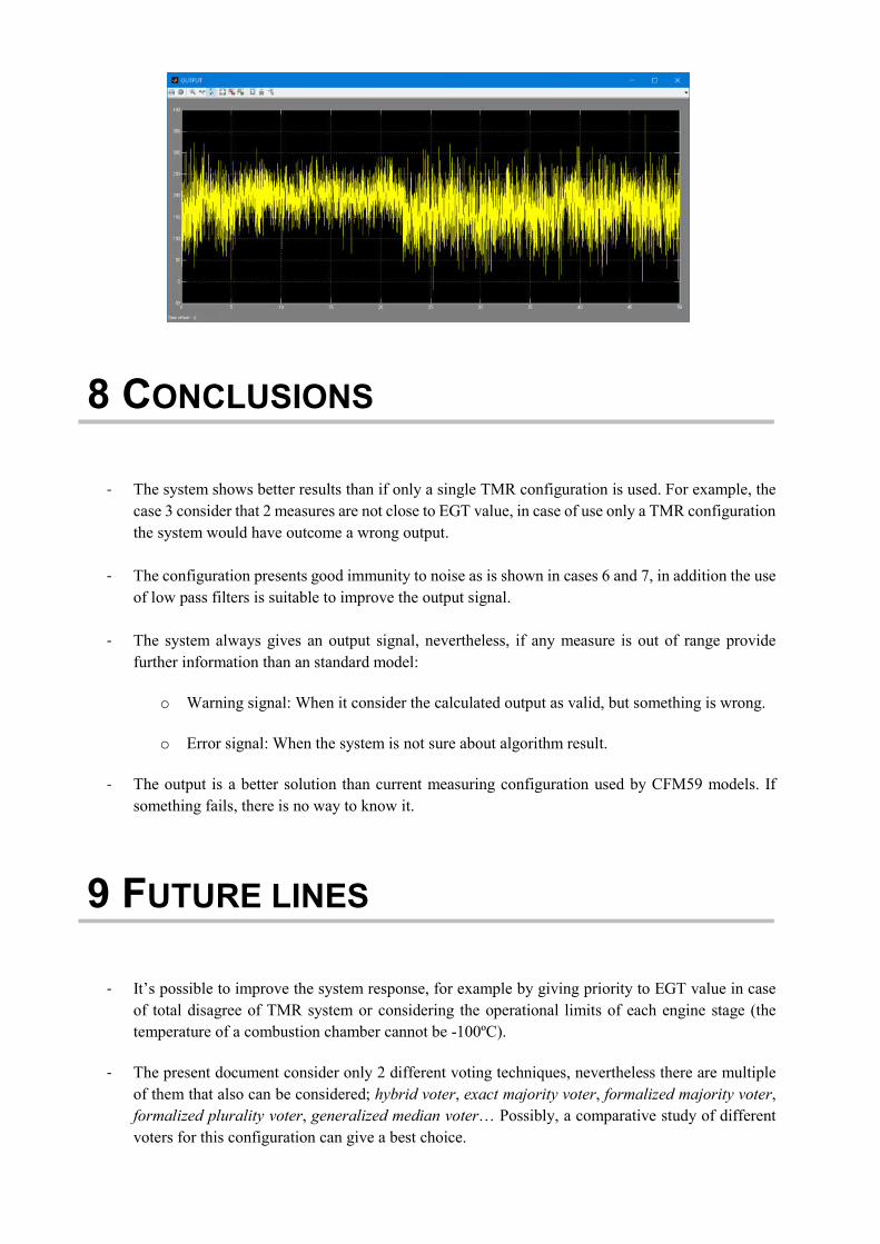
8 CONCLUSIONS

- The system shows better results than if only a single TMR configuration is used. For example, the

case 3 consider that 2 measures are not close to EGT value, in case of use only a TMR configuration

the system would have outcome a wrong output.

- The configuration presents good immunity to noise as is shown in cases 6 and 7, in addition the use

of low pass filters is suitable to improve the output signal.

- The system always gives an output signal, nevertheless, if any measure is out of range provide

further information than an standard model:

o Warning signal: When it consider the calculated output as valid, but something is wrong.

o Error signal: When the system is not sure about algorithm result.

- The output is a better solution than current measuring configuration used by CFM59 models. If

something fails, there is no way to know it.

9 FUTURE LINES

- It’s possible to improve the system response, for example by giving priority to EGT value in case

of total disagree of TMR system or considering the operational limits of each engine stage (the

temperature of a combustion chamber cannot be -100ºC).

- The present document consider only 2 different voting techniques, nevertheless there are multiple

of them that also can be considered; hybrid voter, exact majority voter, formalized majority voter,

formalized plurality voter, generalized median voter… Possibly, a comparative study of different

voters for this configuration can give a best choice.

- Besides TMR, other redundancies configurations can be also considered, as indicated in the

previous point, a comparative study can be made.

- This configuration can be extended to other magnitudes of the aircraft; pressures, voltages,

currents…

10 ANNEXES

9.1 References

R. P. G. Collinson, “Introduction to avionic systems” 3th edition, 2011

Ian Moir, Allan Seabridge, Aircraft systems, mechanical, electrical and avionic subsystem integration, 3th edition, 2008

Chris deLong, The avionics handbook, 2001

Meeting on Integrated Modular Avionics; A380 Integrated Modular Avionics , Rome, Italy, 12th November 2007 (http://www.artist-embedded.org/docs/Events/2007/IMA/Slides/ARTIST2_IMA_Itier.pdf)

Sistemas de navegación, ETSIA, Univ. Politécnica Madrid

International Conference on Advances in Engineering and Technology, Hyderabad

Umamaheswararao Batta, Seetharamaiah Panchumarthy, An improvement in history based weighted voting algorithm, for safety critical systems. Jan-March 2013

G. Latif-Shabgahi, A. J. Hirst, S. Bennett, A novel family of weighted average voters for fault-tolerant computer control systems

Aviónica y sistemas de navegación, ETSI, Univ. Sevilla

Aviónica, ETSI, Univ. Sevilla

B. Umamaheswararao, P. Seetharamaiah, S. Phanikumar, An incorporated voting strategy on majority and score-based fuzzy voting algorithms for safety-critical systems, July 2014

Dominique Briere, Pascal Traverse. Airbus A320/A330/A340 Electrical flight controls, a family of fault-tolerant systems, IEEE 1993.

P. Babul Sahed, K. Subbarao. Performance evaluation of dynamic fuzzy voter used in safety critical systems. International journal of engineering and computer science, August 2013.

CFM56-3 Training manual (http://www.air.flyingway.com/books/engineering/CFM56-3/ctc-142_Line_Maintenance.pdf)

http://en.wikipedia.org/wiki/Acronyms_and_abbreviations_in_avionics

www.modern-avionics.com

http://cursobasicoiva-a.weebly.com/111-evolucioacuten-de-los-sistemas-de-avioacutenica-y-requisitos-de-avioacutenica-en-la-legislacioacuten-aeronaacuteutica.html

http://www.academia.edu/4110287/Instrumentaci%C3%B3n_en_el_sector_aeron%C3%A1utico

https://www.youtube.com/watch?v=zqCRHq2zdEY&list=PLGmKVB7lhqMObYVPz2Jv8pXR-1jDHWciV

http://www.daviddarling.info/encyclopedia/S/STAR.html

https://aviation.stackexchange.com/questions/20739/what-is-a-normal-egt-range-of-a-jet-engine

9.2 List of abbreviations

A/C - Aircraft

ADF - Automatic Direction Finder

ALS – Approach Lighting System

ATA – Air Transport Association

ARNIC – Aeronautical Radio Incorporated

DGPS – Differential GPS

DME – Distance Measuring Equipment

ECU - Engine Control Unit

EPR - Engine Pressure Ratio

EGT – Exhaust Gas Temperature

FADEC - Full Authority Digital Engine Control

GPC – General Purpose Computer

FBW – Fly By Wire

FF - Fuel Flow

FMS – Flight Management System

GPC-General Purpose Computer

GPS – Global Positioning System

IVHM - Integrated Vehicle Health Management

HPC – High Pressure Compressor

HPT – High Pressure Turbine

ILS – Instrumental Landing System

LPC – Low Pressure Compressor

LPT – Low Pressure Turbine

IMA- Integrated Modular Avionics

INS – Inertial Navigation System

MB – Marker Beacon

MLS – Microwave Landing System

MTBF – Mean Time Between Failures

NAV – Air Navigation

NAVAIDS – NAVigation AIDS

NDB – Non Directional Beacon

NMR – N-Modular Redundancy

RNAV – Random or Area Navigation

SAPO – Samocinny Pocitac

SAT – Satellite

SOC - System On a Chip

STAR – Self Testing And Repair

TACAN – Tactical Air Navigation System

TMR – Triple Modular Redundancy

VHF- Very High Frequency

VASIS – Visual Approach Slope Indicator System

VOR – VHF Omni-directional Range

VORTAC – VOR&TACAN

9.3 Matlab function

function [salida, error, warning, debug, contador_coincidencias, aux_out_1, aux_out_2, aux_out_3] = calc_Temp(medida_1, medida_2, medida_3, medida_aux, umbral_1, umbral_2, aux_in_1, aux_in_2, aux_in_3) % This block supports the Embedded MATLAB subset. % See the help menu for details. %************ Inicialización de variables *************** n=3; voto_mayoria=0; contador_coincidencias = 0; salida = 0; error = 0; warning = 0; debug = 0; medida_aux_1 = 0; %******************************************************** %************** uso de variables globales *************** score_1 = aux_in_1; score_2 = aux_in_2; score_3 = aux_in_3; %******************************************************** %Se revisa si las distancias están dentro del umbral de la medida más %fiable (medida_aux) distancia_1aux = abs (medida_1 - medida_aux); distancia_2aux = abs (medida_2 - medida_aux); distancia_3aux = abs (medida_3 - medida_aux); if distancia_1aux <= umbral_2 contador_coincidencias = contador_coincidencias + 1; medida_aux_1 = medida_1; end if distancia_2aux <= umbral_2 contador_coincidencias = contador_coincidencias + 1; medida_aux_1 = medida_aux_1 + medida_2; end if distancia_3aux <= umbral_2 contador_coincidencias = contador_coincidencias + 1; medida_aux_1 = medida_aux_1 + medida_3; end distancia_12 = abs (medida_1 - medida_2); distancia_23 = abs (medida_2 - medida_3); distancia_13 = abs (medida_1 - medida_3); switch contador_coincidencias %Si todas o ninguna están dentro del umbral de la medida fiable, se %calcula la salida con el algoritmo, la diferencia es la señal de error case {0,3} debug = 9; if distancia_12 <= umbral_1 || distancia_13 <= umbral_1 || distancia_23 <= umbral_1 %si entra aquí se puede aplicar el voto por mayoría inexacta, porque al %menos una pareja de medidas están dentro del umbral debug = 2; %Calcula la salida por voto por mayoría inexacta menor_distancia = distancia_12; salida = medida_1; if distancia_12 > distancia_13

menor_distancia = distancia_13; debug = 3; if distancia_12 > distancia_23 salida = medida_3; else salida = medida_1; end if distancia_23 < distancia_13 menor_distancia = distancia_23; salida = medida_2; end else debug = 4; if distancia_12 > distancia_23 menor_distancia = distancia_23; salida = medida_2; debug = 5; if distancia_23 > distancia_13 salida = medida_1; debug = 6; else salida = medida_2; debug = 7; end end end else %Voto por umbral dinamico basado en puntuación con ancho de banda dinámico %************************************************************************* debug = 8; %Normalizar distancias respecto al valor medio vector_distancias = [distancia_12, distancia_13, distancia_23]; distancia_norm_12 = distancia_12/mean(vector_distancias); distancia_norm_13 = distancia_13/mean(vector_distancias); distancia_norm_23 = distancia_23/mean(vector_distancias); %calculo ancho de banda de funcion de membresía %punto central el valor medio, con una anchura de la desviación estándar vector_medidas = [medida_1, medida_2, medida_3]; b = median(vector_medidas); a = std(vector_medidas)- median(vector_medidas); c = std(vector_medidas)+ median(vector_medidas); %Las funciones de membresía (funciones a tramos) serán las siguientes: %x_high = linspace(0,b,1000); %y_high = 1 - (x_high/b); %y_high = ((b-x_high)/(b-a)).*(x_high >= a)+ 1.*(x_high<a); %x_med = linspace(a,c,1000); %y_med = ((x_med-a)/(b-a)).*(x_med<b) + ((x_med-c)/(b-c)).*(x_med>=b); %x_low = linspace(b,c,1000); %Al aplicar cada una de las distancias normalizadas a las funciones de membresía se %obtiene el score de cada una en función de la distancia normalizada ndij: score_1 = score_1 + 1.*(distancia_norm_12<a) + ((b-distancia_norm_12/b)/(b-a).*(distancia_norm_12>=a)) + ((distancia_norm_12-a)/(b-a)).*(distancia_norm_12<b) + ((distancia_norm_12-c)/(b-c)).*(distancia_norm_12>=b) - ((b-distancia_norm_12)/(b-c).*(distancia_norm_12 <= c)) + 1.*(distancia_norm_12>c); score_2 = score_2 + 1.*(distancia_norm_12<a) + ((b-distancia_norm_12/b)/(b-a).*(distancia_norm_12>=a)) + ((distancia_norm_12-a)/(b-a)).*(distancia_norm_12<b) + ((distancia_norm_12-c)/(b-c)).*(distancia_norm_12>=b) - ((b-distancia_norm_12)/(b-c).*(distancia_norm_12 <= c)) + 1.*(distancia_norm_12>c); score_2 = score_2 + 1.*(distancia_norm_23<a) + ((b-distancia_norm_23/b)/(b-a).*(distancia_norm_23>=a)) + ((distancia_norm_23-a)/(b-a)).*(distancia_norm_23<b) + ((distancia_norm_23-c)/(b-c)).*(distancia_norm_23>=b) - ((b-distancia_norm_23)/(b-c).*(distancia_norm_23 <= c)) + 1.*(distancia_norm_23>c); score_3 = score_3 + 1.*(distancia_norm_23<a) + ((b-distancia_norm_23/b)/(b-a).*(distancia_norm_23>=a)) + ((distancia_norm_23-a)/(b-a)).*(distancia_norm_23<b) + ((distancia_norm_23-c)/(b-

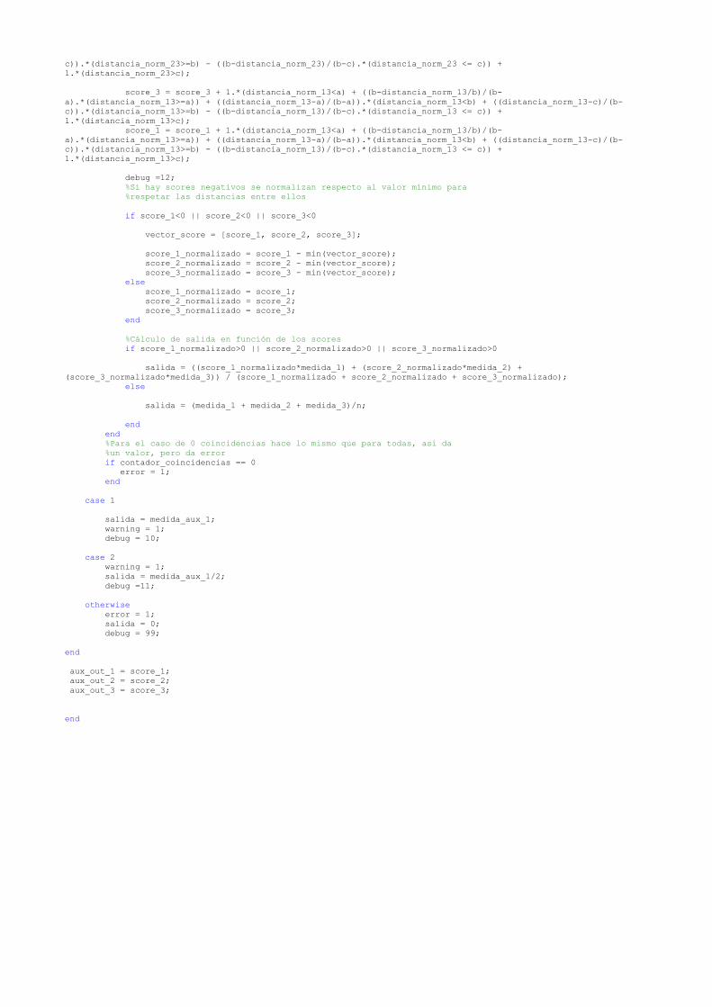
c)).*(distancia_norm_23>=b) - ((b-distancia_norm_23)/(b-c).*(distancia_norm_23 <= c)) + 1.*(distancia_norm_23>c); score_3 = score_3 + 1.*(distancia_norm_13<a) + ((b-distancia_norm_13/b)/(b-a).*(distancia_norm_13>=a)) + ((distancia_norm_13-a)/(b-a)).*(distancia_norm_13<b) + ((distancia_norm_13-c)/(b-c)).*(distancia_norm_13>=b) - ((b-distancia_norm_13)/(b-c).*(distancia_norm_13 <= c)) + 1.*(distancia_norm_13>c); score_1 = score_1 + 1.*(distancia_norm_13<a) + ((b-distancia_norm_13/b)/(b-a).*(distancia_norm_13>=a)) + ((distancia_norm_13-a)/(b-a)).*(distancia_norm_13<b) + ((distancia_norm_13-c)/(b-c)).*(distancia_norm_13>=b) - ((b-distancia_norm_13)/(b-c).*(distancia_norm_13 <= c)) + 1.*(distancia_norm_13>c); debug =12; %Si hay scores negativos se normalizan respecto al valor mínimo para %respetar las distancias entre ellos if score_1<0 || score_2<0 || score_3<0 vector_score = [score_1, score_2, score_3]; score_1_normalizado = score_1 - min(vector_score); score_2_normalizado = score_2 - min(vector_score); score_3_normalizado = score_3 - min(vector_score); else score_1_normalizado = score_1; score_2_normalizado = score_2; score_3_normalizado = score_3; end %Cálculo de salida en función de los scores if score_1_normalizado>0 || score_2_normalizado>0 || score_3_normalizado>0 salida = ((score_1_normalizado*medida_1) + (score_2_normalizado*medida_2) + (score_3_normalizado*medida_3)) / (score_1_normalizado + score_2_normalizado + score_3_normalizado); else salida = (medida_1 + medida_2 + medida_3)/n; end end %Para el caso de 0 coincidencias hace lo mismo que para todas, así da %un valor, pero da error if contador_coincidencias == 0 error = 1; end case 1 salida = medida_aux_1; warning = 1; debug = 10; case 2 warning = 1; salida = medida_aux_1/2; debug =11; otherwise error = 1; salida = 0; debug = 99; end aux_out_1 = score_1; aux_out_2 = score_2; aux_out_3 = score_3; end