Providing Location-Privacy in Opportunistic Mobile Social ... · Abstract Users face...
118
Providing Location-Privacy in Opportunistic Mobile Social Networks by Rui Huang Thesis submitted in partial fulfillment of the requirements for the Master of Applied Science degree in Electrical and Computer Engineering Ottawa-Carleton Institute of Electrical and Computer Engineering School of Electrical Engineering and Computer Science University of Ottawa Rui Huang, Ottawa, Canada, 2018
Transcript of Providing Location-Privacy in Opportunistic Mobile Social ... · Abstract Users face...

Providing Location-Privacy inOpportunistic Mobile Social
Networks
by
Rui Huang
Thesis submitted in partial fulfillment of the requirementsfor the Master of Applied Science degree in
Electrical and Computer Engineering
Ottawa-Carleton Institute of Electrical and Computer EngineeringSchool of Electrical Engineering and Computer Science
University of Ottawa
© Rui Huang, Ottawa, Canada, 2018

Abstract
Users face location-privacy risks when accessing Location-Based Services (LBSs) in an Op-
portunistic Mobile Social Networks (OMSNs). In order to protect the original requester’s
identity and location, we propose two location privacy obfuscation protocols utilizing social
ties between users.
The first one is called Multi-Hop Location-Privacy Protection (MHLPP) protocol. To
increase chances of completing obfuscation operations, users detect and make contacts with
one-hop or multi-hop neighbor friends in social networks. Encrypted obfuscation queries
avoid users learning important information especially the original requester’s identity and
location except for trusted users. Simulation results show that our protocol can give a
higher query success ratio compared to its existing counterpart.
The second protocol is called Appointment Card Protocol (ACP). To facilitate the
obfuscation operations of queries, we introduce the concept called Appointment Card (AC).
The original requesters can send their queries to the LBS directly using the information
in the AC, ensuring that the original requester is not detected by the LBS. Also, a path
for reply message is kept when the query is sent, to help reduce time for replying queries.
Simulation results show that our protocol preserves location privacy and has a higher query
success ratio than its counterparts.
We have also developed a new OMSN simulator, called OMSN Routing Simulator
(ORS), for simulating OMSN protocols more efficiently and effectively for reliable perfor-
mance.
ii

Acknowledgements
First, I would like to express my sincere gratitude to Prof. Amiya Nayak for his continuous
support, motivation, advice and immense knowledge throughout my thesis work. I could
not have imagined having a better mentor for my Master’s study.
Also, I would like to thank my family and friends, especially Yichao Lin, for providing
me with unfailing support and encouragement throughout the process of researching and
writing my thesis. This accomplishment would not have been possible without them.
Thank you.
iii

Table of Contents
List of Tables viii
List of Figures x
1 Introduction 1
1.1 Motivation and Objective . . . . . . . . . . . . . . . . . . . . . . . . . . . 1
1.2 Objectives . . . . . . . . . . . . . . . . . . . . . . . . . . . . . . . . . . . . 3
1.3 Contributions . . . . . . . . . . . . . . . . . . . . . . . . . . . . . . . . . . 3
1.4 Thesis Organization . . . . . . . . . . . . . . . . . . . . . . . . . . . . . . . 4
2 Background and Related Work 6
2.1 Mobile Ad hoc Networks . . . . . . . . . . . . . . . . . . . . . . . . . . . . 6
2.2 Delay Tolerant Network . . . . . . . . . . . . . . . . . . . . . . . . . . . . 7
2.2.1 Spray and Wait Protocol . . . . . . . . . . . . . . . . . . . . . . . 8
2.2.2 Other DTN Protocols . . . . . . . . . . . . . . . . . . . . . . . . . 9
2.3 Location-Based Services . . . . . . . . . . . . . . . . . . . . . . . . . . . . 10
2.4 Social Networks . . . . . . . . . . . . . . . . . . . . . . . . . . . . . . . . . 11
2.5 Location-Privacy Protocols . . . . . . . . . . . . . . . . . . . . . . . . . . . 12
iv

2.5.1 Centralized Protocols . . . . . . . . . . . . . . . . . . . . . . . . . 12
2.5.2 Distributed Protocols . . . . . . . . . . . . . . . . . . . . . . . . . 16
3 Multi-Hop Location-Privacy Protection 18
3.1 System Model . . . . . . . . . . . . . . . . . . . . . . . . . . . . . . . . . . 18
3.2 Details of MHLPP . . . . . . . . . . . . . . . . . . . . . . . . . . . . . . . 19
3.3 Requirement parameters . . . . . . . . . . . . . . . . . . . . . . . . . . . . 22
3.4 Privacy Analysis . . . . . . . . . . . . . . . . . . . . . . . . . . . . . . . . 26
3.5 Complexity discussion . . . . . . . . . . . . . . . . . . . . . . . . . . . . . 27
3.6 Performance Analysis . . . . . . . . . . . . . . . . . . . . . . . . . . . . . . 28
3.6.1 Query success ratio . . . . . . . . . . . . . . . . . . . . . . . . . . 30
3.6.2 Number of Hops . . . . . . . . . . . . . . . . . . . . . . . . . . . . 32
3.6.3 Security . . . . . . . . . . . . . . . . . . . . . . . . . . . . . . . . . 34
4 Appointment Card Protocol 37
4.1 System Model . . . . . . . . . . . . . . . . . . . . . . . . . . . . . . . . . . 37
4.2 Appointment Card Protocol Overview . . . . . . . . . . . . . . . . . . . . 38
4.3 Appointment Card . . . . . . . . . . . . . . . . . . . . . . . . . . . . . . . 41
4.4 AC Life Cycle . . . . . . . . . . . . . . . . . . . . . . . . . . . . . . . . . . 42
4.5 System Parameters . . . . . . . . . . . . . . . . . . . . . . . . . . . . . . . 43
4.5.1 Obfuscation Distance . . . . . . . . . . . . . . . . . . . . . . . . . . 43
4.5.2 Friends Obfuscation Distance . . . . . . . . . . . . . . . . . . . . . 44
4.5.3 Generating Period . . . . . . . . . . . . . . . . . . . . . . . . . . . 45
v

4.5.4 Distributing Segment . . . . . . . . . . . . . . . . . . . . . . . . . . 45
4.5.5 Avoiding Time . . . . . . . . . . . . . . . . . . . . . . . . . . . . . 46
4.5.6 AC Timeout . . . . . . . . . . . . . . . . . . . . . . . . . . . . . . . 46
4.6 Protocol Details . . . . . . . . . . . . . . . . . . . . . . . . . . . . . . . . . 47
4.6.1 Generating ACs . . . . . . . . . . . . . . . . . . . . . . . . . . . . . 47
4.6.2 Exchange Distributing Appointment Cards . . . . . . . . . . . . . . 48
4.6.3 Exchange Ready Appointment Cards . . . . . . . . . . . . . . . . . 49
4.6.4 Sending Queries . . . . . . . . . . . . . . . . . . . . . . . . . . . . . 50
4.6.5 Sending Replies . . . . . . . . . . . . . . . . . . . . . . . . . . . . . 52
4.7 Appointment Number . . . . . . . . . . . . . . . . . . . . . . . . . . . . . 58
4.7.1 Creator Appointment Number . . . . . . . . . . . . . . . . . . . . . 58
4.7.2 Agent Appointment Number . . . . . . . . . . . . . . . . . . . . . . 59
4.7.3 Timeout . . . . . . . . . . . . . . . . . . . . . . . . . . . . . . . . . 59
4.8 Example . . . . . . . . . . . . . . . . . . . . . . . . . . . . . . . . . . . . 60
4.8.1 Exchanging Appointment Cards . . . . . . . . . . . . . . . . . . . 62
4.8.2 Queries and Replies . . . . . . . . . . . . . . . . . . . . . . . . . . 74
4.9 Experiment . . . . . . . . . . . . . . . . . . . . . . . . . . . . . . . . . . . 77
4.9.1 Average Query Success Ratio . . . . . . . . . . . . . . . . . . . . . 78
4.9.2 Average Reply Success Ratio . . . . . . . . . . . . . . . . . . . . . 81
4.9.3 Total Number of Query Relays . . . . . . . . . . . . . . . . . . . . 82
4.9.4 Memory Cost . . . . . . . . . . . . . . . . . . . . . . . . . . . . . . 84
4.9.5 Distributing Appointment Cards . . . . . . . . . . . . . . . . . . . 85
vi

5 OMSN Routing Simulator (ORS) 88
5.1 Overview . . . . . . . . . . . . . . . . . . . . . . . . . . . . . . . . . . . . . 89
5.2 Vertex Reduction Algorithm . . . . . . . . . . . . . . . . . . . . . . . . . . 91
5.2.1 Ignorable Vertex and Reserved Vertex . . . . . . . . . . . . . . . . 92
5.2.2 Vertex Reduction . . . . . . . . . . . . . . . . . . . . . . . . . . . 95
5.2.3 Assembling Vertices . . . . . . . . . . . . . . . . . . . . . . . . . . 96
5.3 Finding Nodes in a Range . . . . . . . . . . . . . . . . . . . . . . . . . . . 98
5.3.1 Static Nodes . . . . . . . . . . . . . . . . . . . . . . . . . . . . . . 99
5.3.2 Mobile Nodes . . . . . . . . . . . . . . . . . . . . . . . . . . . . . . 99
5.3.3 Complexity . . . . . . . . . . . . . . . . . . . . . . . . . . . . . . . 100
6 Conclusion and Future Work 101
6.1 Summary of Work Done . . . . . . . . . . . . . . . . . . . . . . . . . . . . 101
6.2 Future Work . . . . . . . . . . . . . . . . . . . . . . . . . . . . . . . . . . 102
vii

List of Tables
3.1 MHLPP Symbols . . . . . . . . . . . . . . . . . . . . . . . . . . . . . . . . 20
3.2 MHLPP Experiment Parameters . . . . . . . . . . . . . . . . . . . . . . . 28
4.1 ACP Symbols . . . . . . . . . . . . . . . . . . . . . . . . . . . . . . . . . . 40
4.2 Appointment Card . . . . . . . . . . . . . . . . . . . . . . . . . . . . . . . 42
4.3 Important System Parameters . . . . . . . . . . . . . . . . . . . . . . . . . 43
4.4 Relay Table Entries . . . . . . . . . . . . . . . . . . . . . . . . . . . . . . . 49
4.5 Reply Table Entries of The First Agent . . . . . . . . . . . . . . . . . . . . 53
4.6 Reply Table Entries of The Second Agent . . . . . . . . . . . . . . . . . . . 55
4.7 Reply Table Entries of The Last Agent . . . . . . . . . . . . . . . . . . . . 56
4.8 Example Parameters . . . . . . . . . . . . . . . . . . . . . . . . . . . . . . 60
4.9 Example Event . . . . . . . . . . . . . . . . . . . . . . . . . . . . . . . . . 61
4.10 Example Initial State . . . . . . . . . . . . . . . . . . . . . . . . . . . . . . 61
4.11 User X and Y’s AC Lists . . . . . . . . . . . . . . . . . . . . . . . . . . . . 62
4.12 Elizabeth and Bob’s AC Lists at Time t1 . . . . . . . . . . . . . . . . . . . 63
4.13 Elizabeth and Bob’s Relay Table At Time t1 . . . . . . . . . . . . . . . . . 63
4.14 Bob and Charlie’s AC Lists at Time t2 . . . . . . . . . . . . . . . . . . . . 64
viii

4.15 Bob and Charlie’s Relay Table At Time t2 . . . . . . . . . . . . . . . . . . 64
4.16 Charlie and Elizabeth’s AC Lists at Time t3 . . . . . . . . . . . . . . . . . 65
4.17 Charlie and Elizabeth’s Relay Table At Time t3 . . . . . . . . . . . . . . . 66
4.18 Elizabeth and Alice’s AC Lists at Time t4 . . . . . . . . . . . . . . . . . . 67
4.19 Elizabeth and Alice’s Relay Table At Time t4 . . . . . . . . . . . . . . . . 67
4.20 Bob and Charlie’s AC Lists at Time t5 . . . . . . . . . . . . . . . . . . . . 68
4.21 Bob and Charlie’s Relay Table At Time t5 . . . . . . . . . . . . . . . . . . 69
4.22 Alice and Charlie’s AC Lists at Time t6 . . . . . . . . . . . . . . . . . . . . 70
4.23 Alice and Charlie’s Relay Table At Time t6 . . . . . . . . . . . . . . . . . . 70
4.24 Charlie and David’s AC Lists at Time t7 . . . . . . . . . . . . . . . . . . . 71
4.25 Charlie and David’s Relay Table At Time t7 . . . . . . . . . . . . . . . . . 72
4.26 David and Elizabeth’s AC Lists at Time t8 . . . . . . . . . . . . . . . . . . 73
4.27 David and Elizabeth’s Relay Table At Time t8 . . . . . . . . . . . . . . . . 74
4.28 Elizabeth’s Reply Table Entry . . . . . . . . . . . . . . . . . . . . . . . . . 75
4.29 Bob’s Reply Table Entry . . . . . . . . . . . . . . . . . . . . . . . . . . . . 76
4.30 Charlie’s Reply Table Entry . . . . . . . . . . . . . . . . . . . . . . . . . . 77
ix

List of Figures
2.1 MANET . . . . . . . . . . . . . . . . . . . . . . . . . . . . . . . . . . . . . 7
2.2 The comparison between regular networks and DTNs . . . . . . . . . . . . 8
2.3 LBS [23] . . . . . . . . . . . . . . . . . . . . . . . . . . . . . . . . . . . . . 11
2.4 Single Anonymization Server . . . . . . . . . . . . . . . . . . . . . . . . . . 14
2.5 REAL [7] . . . . . . . . . . . . . . . . . . . . . . . . . . . . . . . . . . . . 15
3.1 The Selection Of The Next Friend . . . . . . . . . . . . . . . . . . . . . . . 24
3.2 The Number Of Encryption With Various Inner Radius . . . . . . . . . . . 27
3.3 The Query Success Ratio Comparison Between HSLPO and MHLPP . . . 31
3.4 The Number Of Hops Comparison Between HSLPO And MHLPP . . . . . 33
3.5 Locating Probability Entropy Comparison Between HSLPO And MHLPSP 36
4.1 Example of ACP Message Exchange . . . . . . . . . . . . . . . . . . . . . . 39
4.2 AC’s Life Cycle . . . . . . . . . . . . . . . . . . . . . . . . . . . . . . . . . 43
4.3 Obfuscation Distance . . . . . . . . . . . . . . . . . . . . . . . . . . . . . . 44
4.4 Friends-Obfuscation Distance . . . . . . . . . . . . . . . . . . . . . . . . . 45
4.5 Constitute Query . . . . . . . . . . . . . . . . . . . . . . . . . . . . . . . . 52
4.6 Constitute Replies . . . . . . . . . . . . . . . . . . . . . . . . . . . . . . . 53
x

4.7 The Reply of The First Agent . . . . . . . . . . . . . . . . . . . . . . . . . 54
4.8 The Reply of The Second Agent . . . . . . . . . . . . . . . . . . . . . . . . 55
4.9 The Reply of the Last Agent . . . . . . . . . . . . . . . . . . . . . . . . . . 57
4.10 David’s Query . . . . . . . . . . . . . . . . . . . . . . . . . . . . . . . . . . 75
4.11 Elizabeth Forwards A Reply . . . . . . . . . . . . . . . . . . . . . . . . . . 76
4.12 Bob Forwards A Reply . . . . . . . . . . . . . . . . . . . . . . . . . . . . . 76
4.13 Charlie Forwards A Reply . . . . . . . . . . . . . . . . . . . . . . . . . . . 77
4.14 Average Query Success Ratio (at 10 minutes mark) . . . . . . . . . . . . . 79
4.15 Average Query Success Ratio (at 20 minutes mark) . . . . . . . . . . . . . 80
4.16 Average Query Success Ratio for 50-Meters Communication Range . . . . 81
4.17 Average Reply Success Ratio for 50-Meters Communication Range . . . . . 82
4.18 Average Number of Forwarding Queries At 20 Minutes Mark . . . . . . . . 83
4.19 Average Number of Query Buffer Needed at 20 Minutes Mark . . . . . . . 84
4.20 Average Number of Queries Carried Per User . . . . . . . . . . . . . . . . 86
4.21 Average Number of Exchanging ACs Per Minute Under Different Commu-
nication Ranges . . . . . . . . . . . . . . . . . . . . . . . . . . . . . . . . . 87
4.22 Average Number of Ready ACs Per User . . . . . . . . . . . . . . . . . . . 87
5.1 Simulator UI . . . . . . . . . . . . . . . . . . . . . . . . . . . . . . . . . . 90
5.2 Shortest Path On A Single Segment-Line . . . . . . . . . . . . . . . . . . . 93
5.3 Remove Ignorable Vertices . . . . . . . . . . . . . . . . . . . . . . . . . . . 95
5.4 Tidy Reserved Connections . . . . . . . . . . . . . . . . . . . . . . . . . . 96
5.5 Grid Size For Still Nodes . . . . . . . . . . . . . . . . . . . . . . . . . . . . 99
5.6 Length of Grid . . . . . . . . . . . . . . . . . . . . . . . . . . . . . . . . . 100
xi

Chapter 1
Introduction
Location-privacy is becoming a major concern in the Opportunistic Mobile Social Network
(OMSN, which is a kind of a Delay Tolerant Network (DTN) [6] featuring lack of continuous
connectivity. More specifically, in OMSNs, it is not necessary for senders to have an end-
to-end routing path to their destinations. Users make contact when they encounter each
other. LBSs are common applications in OMSNs and they are widely used in “military
and government industries, emergency services and the commercial sector” [24], especially
after the proliferation of localization technologies, like GPS. Many people access LBSs with
their portable devices and send their location to LBS providers. In this case, LBS users
face a continuous risk that their location may be leaked from the LBS applications, which
makes people unwilling to use LBSs. Thus, protecting location privacy has been a critical
issue in LBSs.
1.1 Motivation and Objective
LBSs which use the location information of users can be considered as “two types of appli-
cation design: push and pull services” [24]. For example, you may receive an advertisement
when you enter an area, which is a push service; if you look for the nearest restaurant, you
1

must pull information from the network. It is obvious that you must reveal your location
if you use LBS. When you use a LBS application to find the nearest restaurant, you ac-
tually tell the LBS provider your location and your next destination which might have a
restaurant nearby. If attackers can access the LBS provider’s database, they can learn that
information. Then you may receive a lot of advertisements from surrounding restaurants.
Such inference attack, in addition to bothering you with advertisements, can become
more dangerous when you send more queries to the LBS provider. If you use an LBS ap-
plication several times in a day, the attackers can learn your trace from the information so
that they can infer more information including your identity and home address. According
to [12], “Hoh used a database of week-long GPS traces from 239 drivers in the Detroit,
MI area. Examining a subset of 65 drivers, their home-finding algorithm was able to find
plausible home locations of about 85%, although the authors did not know the actual loca-
tions of the drivers’ homes”. Therefore, the LBS provider is considered as a semi-trusted
party so that users must protect their location-privacy when they use LBS applications.
The OMSN is defined “as decentralized opportunistic communication networks formed
among human carried mobile devices that take advantage of mobility and social networks to
create new opportunities for exchanging information and mobile ad hoc social networking”
[22]. In other words, OMSN is a kind of mobile ad hoc network, and the information and
technology of social network are also used in it. People carrying smartphones which contain
WiFi or Bluetooth can form a typical OMSN. Since the WiFi, Bluetooth on smartphones
can be used for discovering other devices and direct communication between devices, users
can communicate with others who are within their communication range without using
any infrastructure, which is the basic requirement of an OMSN. Since users in OMSN
could also use LBS applications, their location-privacy must be protected. Besides, the
information in the social network allows users to identify friends. Therefore, it is necessary
to have location-privacy protection protocol using the social networks.
2

1.2 Objectives
Disconnection, decentralization and highly delays are obvious features for OMSN so that a
decentralized strategy may benefit for the location-privacy protection protocol in OMSN.
Besides, decreasing interactions between users and servers can significantly cut down the
time cost. To prevent the attackers from learning users’ private information, the protocol
should obfuscate users’ location and hide their identities.
1.3 Contributions
We propose two new decentralized location-privacy protecting protocols for OMSN so that
they do not need a three-party server which is used to obfuscate queries for users. We also
create a new simulator for OMSNs called OMSN Routing protocols Simulator (ORS) to
evaluate our protocols.
The first protocol we propose is a distributed location-privacy algorithm called Multi-
Hop Location-Privacy Protection (MHLPP), which achieves a higher query success ratio
and guarantees location-privacy. The introduction of social networks enables us to hide
the original requester’s information behind his friends. When a user wants to send a
query, he starts to look for friends based on information in his social network. He sends
his query to the first encountered friend who is then responsible for forwarding the query
to the intended location. This friend can also pass the query to one of his friends when
they encounter. When the distance between the user carrying this query and the original
requester exceeds a specified threshold, the user sends the query to the LBS server directly
without having to find a friend to pass on. At that time, he also replaces the original
requester’s information with its own identity and location, which enables the LBS server
to receive the query without any information about the original requester. After receiving
the query, the LBS server replies to the last friend (the user sending the query to the LBS)
3

who then transmits it to the original requester.
Our second protocol is also a distributed location-privacy algorithm called Appointment
Card Protocol (ACP), which aims to guarantee location-privacy and reach a higher query
success ratio. The introduction of social networks enables us to hide the original requester’s
information behind his friends. We introduce the Appointment Card (AC) as a kind of
intermediary which records a series of agents. The original requester sends his query using
the identity of the first agent in the AC to the LBS, which prevents the LBS from learning
the identity of the requester. The reply of the query can be delivered back to the original
requester through the same series of agents as in the AC. The last agent, called the trusted
agent, is a user of the original requester, in the social network; in other words, he is a
friend (or a friend of friends) of the original requester. The trusted agent separates the
stranger-agents from the original requester so that no stranger knows the identity of the
original requester. The query-delivery success ratio of our ACP is as good as that of any
no-privacy protocol used in comparison in our experiment.
Our new simulator ORS is inspired by a well-known simulator, ONE [11], which is used
by many researchers to test their models and protocols in DTN. The major reason why
we created a new simulator is that the ONE is not designed for OMSN and lacks social
networking concepts for it to be effective in OMSN. Adding social network information
into the ONE simulator must modify its basic structure, which is problematic and might
not ensure correctness of our experiments. We used more efficient algorithms to make our
simulator run two times faster than ONE.
1.4 Thesis Organization
This thesis is organized as follows:
Chapter 2 describes the concept of Mobile Ad hoc networks, Delay Tolerant Networks,
4
Location-Based Services and social networks. We also give an overview of the existing
location-privacy protocols.
Chapter 3 describes our first protocol, MHLPP, in detail. The performance of MHLPP
has been compared against its counterpart, Hybrid and Social-aware Location-Privacy in
Opportunistic mobile social networks (HSLPO) [31].
Chapter 4 elaborates on the second protocol, ACP. We describe how it works and how
it enhances the location-privacy. Its performance is compared against Binary Spray and
Wait (BSW) [25], distributed social based location privacy protocol (SLPD) [30], and our
Multi-Hop Location-Privacy Protection (MHLPP).
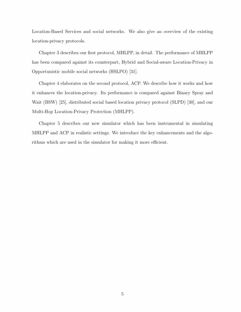
Chapter 5 describes our new simulator which has been instrumental in simulating
MHLPP and ACP in realistic settings. We introduce the key enhancements and the algo-
rithms which are used in the simulator for making it more efficient.
5
Chapter 2
Background and Related Work
2.1 Mobile Ad hoc Networks
“Ad hoc networks are infrastructure-less and cooperation-based networks which means
that the network topologies must be decided by the network sensors themselves” [33]. In
other words, the major feature of ad hoc networks is that they have no infrastructures.
The Mobile Ad hoc NETwork (MANET), also called the Wireless Ad hoc NETwork
(WANET), is a decentralized wireless network with no pre-existing infrastructure. In
MANET, because users move independently, the topology changes frequently. Without
the help of infrastructure, users can only communicate when they encounter each other.
In other words, users communicate only if they are covered by each other’s communication
range. Because of the above characteristics, the MANET can be viewed as a kind of Delay-
Tolerant Network (DTN) that lacks continuous network connectivity. The MANET can
hardly establish instantaneous end-to-end paths, which compels the routing protocols in
MANET to use a “store-and-forward” strategy in which users forward messages when they
encounter others, or they store messages for later delivery. As shown in Figure 2.1, the
user A has a message for C but does not know where C is, so he sends the message to B
when they encounter each other. The user B then stores the message and moves along.
6

The message is then delivered to C when both B and C come in contact with each other
at a later time. It is obvious that whether the message can be delivered depends on the
movement of the users. If B will never meet C or the message is held by a user for a long
period of time, it must be dropped after some timeout. The delivery process can lead to
low success ratio and is often time-consuming.
Figure 2.1: MANET
2.2 Delay Tolerant Network
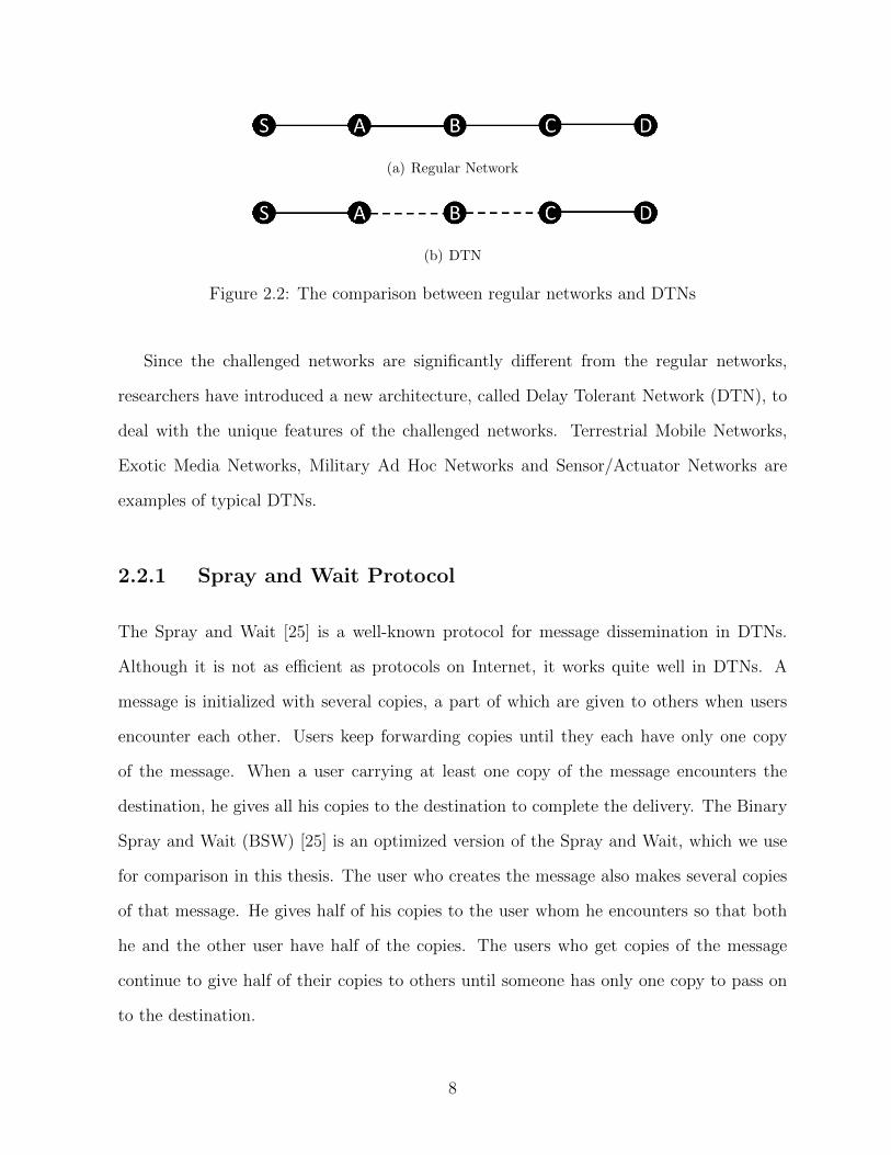
Regular networks, e.g. Internet, always have end-to-end paths. As shown in Figure 2.2(a),
two nodes S and D are connected through nodes A, B, and C. The maximum round-trip
time is not excessive, and their drop probability is also small. Compared to the regular
network, there is a class of challenged networks [6] which lack end-to-end path and suffer
from high latency and long queuing delays. As shown in Figure 2.2(b), when node B is
down or non-existent, there is no connection between nodes A and C, for which extensive
latency is inevitable if the source S sends a message to the destination D.
7
(a) Regular Network
(b) DTN
Figure 2.2: The comparison between regular networks and DTNs
Since the challenged networks are significantly different from the regular networks,
researchers have introduced a new architecture, called Delay Tolerant Network (DTN), to
deal with the unique features of the challenged networks. Terrestrial Mobile Networks,
Exotic Media Networks, Military Ad Hoc Networks and Sensor/Actuator Networks are
examples of typical DTNs.
2.2.1 Spray and Wait Protocol
The Spray and Wait [25] is a well-known protocol for message dissemination in DTNs.
Although it is not as efficient as protocols on Internet, it works quite well in DTNs. A
message is initialized with several copies, a part of which are given to others when users
encounter each other. Users keep forwarding copies until they each have only one copy
of the message. When a user carrying at least one copy of the message encounters the
destination, he gives all his copies to the destination to complete the delivery. The Binary
Spray and Wait (BSW) [25] is an optimized version of the Spray and Wait, which we use
for comparison in this thesis. The user who creates the message also makes several copies
of that message. He gives half of his copies to the user whom he encounters so that both
he and the other user have half of the copies. The users who get copies of the message
continue to give half of their copies to others until someone has only one copy to pass on
to the destination.
8

2.2.2 Other DTN Protocols
2.2.2.1 Direct Contact Scheme
The simplest strategy for DTN is that the source holds the message until he meets the
destination, which is called the direct contact scheme. So, a direct path between the source
and the destination is necessary for a successful delivery. It is possible that the source never
comes in contact with the destination in which case the message is not delivered.
2.2.2.2 Replica Based Protocols
The replica based protocols (e.g., [9], [13], [27], [15], and [20]) work by making several
replicas of the message so that users can retransmit them upon connection establishment.
The former BSW is also a kind of replica based protocols. Compared to the direct contact
scheme, the replica-based protocols make it easy for messages to be delivered. But, they
require more resources than the direct contact scheme because they need more memory to
store the replicas. Therefore, making a reasonable decision on the message replication is
the key to success of these kinds of protocols.
2.2.2.3 Knowledge-Based Protocols
Different from the former replica protocols which require no knowledge about the topology
of the network, the users in knowledge-based protocols try to evaluate their own view of
the topology of the network so that they can make better forwarding decisions, e.g. [29],
[10] and [16]. However, the topology changes so frequently that it is hard for users to have
an accurate topology.
9

2.2.2.4 Coding Based Protocols
Authors in [14] and [2] have suggested the approach that introduces coding techniques into
the routing protocols. Instead of making a few replicas, coding based protocols encrypt
data to make a large number of message blocks. If the destination receives a part of the
blocks, he can decrypt the message.
2.3 Location-Based Services
The Location-Based Services (LBS) use users’ location information to provide services as
shown in Figure 2.3. Your smartphone can detect your coordinate and send it to LBS
application server which is responsible for providing service based on the coordinate. The
point of interest and the location advertisement are familiar instances of LBS. The LBS
providers collect users’ location information to provide service, which makes LBS providers
a significant target of attack. When attackers access the databases of the LBS providers,
they can learn all sensitive information in the servers. So, the LBS providers should be
viewed as semi-trusted, which might expose information in front of vicious attackers.
Users face risks of information breach when they access a semi-trusted LBS provider
because anyone who has access to data in LBSs is able to steal and misuse LBS users’
location-privacy. Considering that LBSs rely on location-aware computing, it is unavoid-
able to leak users’ location from LBSs. Therefore, balancing “these two competing aims of
location privacy and location awareness” [4] is always a challenge.
10

Figure 2.3: LBS [23]
2.4 Social Networks
Social networks which contain social interactions and personal relationships are used in
location-privacy protection so that users can determine who can or cannot be trusted. In
[28], the relationship of a pair of people (e.g., user i and user j) is described as a pair of
directed relationship strength. The directed relationship strength from the user i to the
user j can be denoted by RSij. We should notice that RSij might not be equal to RSji,
because the user i might like the user j very much while the user j just views the user
i as an acquaintance. Based on the relationship strength, it is possible to estimate the
relational tie between two people and predict whether they are friends or strangers.
The relationship strength is compared with a threshold; if the relationship strength is
higher than the threshold then the two people are friends, otherwise they are strangers. In
the protocols we mention in the thesis, researchers always assume that friends are trustful.
That is reasonable because you might feel more secure when your friends forward your
message instead of a stranger.
11

2.5 Location-Privacy Protocols
The basic idea of most location-privacy protocols is hiding the original requester behind a
set of users so that attackers can hardly infer the identity of the original requester. In other
words, when a user sends a query, his identity cannot be inferred based on the information
in the query easily. For example, the original requester can use a pseudonym instead of his
real name or use an obfuscated location to send his queries, so that attackers cannot tell
the difference between two sets of queries.
The location-privacy protocols are considered centralized and distributed based on
whether they require any infrastructure for operation.
2.5.1 Centralized Protocols
Centralized protocols always need some infrastructure for the obfuscation process. The
infrastructure could be any equipment which acts as an anonymization server. When the
user wants to send a query to the LBS server, he sends the query to the anonymization
server. The anonymization server changes the identity and the location in the query,
which is called anonymization or obfuscation. Then, the anonymization server forwards
the modified query to the LBS server, so that the attacker who attacks the LBS server
can hardly learn the identity of the original requester. The LBS server can send the reply
message to the anonymization server which is responsible for forwarding the reply message
back to the original requester. In this way, the original requester gets the information he
needs, while avoiding from being located by the attackers.
The advantage of a centralized protocol is that the anonymization server has more
resources and information than users in the network, which enable the server to achieve
better anonymization performance and provide sufficient protection for users. For example,
if the anonymization server knows locations of all users in the network, it can modify the
12

location and identity in the queries to the most suitable, with which the LBS server can
provide acceptable results while the original requester is not exposed.
There are two major shortcomings of these kinds of protocols: i) it is hard to deploy
infrastructure in some areas, ii) since the anonymization server knows users’ location, it is
also a risk for the users.
2.5.1.1 Single Server
Authors in [18] use a central anonymity server through which the mobile users can send
queries to LBS. To make the communication between users and the central anonymity
server trustful, users set up an encrypted connection with the anonymity server at the be-
ginning. Users sends their encrypted queries to the anonymity server, so that the anonymity
server is the only one who can learn the information in the query. The anonymity server
decrypts the queries and uses a cloaking algorithm to perturb the position information in
the queries. Then the anonymity server sends the modified queries to external services
(e.g., LBS). This is a typical centralized protocol, which can reduce the re-identification
risk for the users. Its drawback is that a continuous connection to the server is necessary
for each user, which is hard to achieve in a sparse DTN. We cannot also assume that a
MANET user can have a stable connection with a central anonymity server either.
In [19], researchers employ a matchmaker which is used to match users and advertise-
ments, by which users can achieve anonymization of their identities and locations from the
matchmaker. The system architecture in [19] is similar to the former [18], while authors
in [19] just focus on the advertisement service instead of the “external services” in [18].
The role of the matchmaker is simply matching users and advertisements. Although the
functions of the matchmaker in [19] and the central anonymity server in [18] are differ-
ent, the intermediate trusted three-party servers (i.e., the matchmaker and the central
anonymity server) separate users and the application server (e.g., an advertisement server,
13

LBS server). The architecture in [19] does not require an encryption process, so the at-
tackers can learn the information in the queries. When a large number of queries arrive
at the matchmaker in a short time from different users, it helps the matchmaker mix the
queries so that attackers can hardly trace the query, but the burden of the users who are
near the matchmaker can be heavy.
In [26], researchers use a trusted, third-party location anonymization engine (LAE)
that acts as a middle layer between mobile users and the LBS provider, in which exact
locations and requests from clients are replaced by a location anonymization engine before
they arrive at the LBS provider. Therefore, it appears that the suggest approach is almost
like that shown in Figure 2.4. A trusted server is placed between users and the application
server, which hides users’ information and offers sufficient information for the application
servers to provide acceptable service.
Figure 2.4: Single Anonymization Server
2.5.1.2 Multiple Servers
The above protocols always use a single anonymization server, while there are other pro-
tocols which need multiple infrastructures.
Authors in [17] propose a protocol, called Social-based PRivacy-preserving packet for-
wardING (SPRING), for vehicular delay-tolerant network. In their work, they employ
Roadside Units (RSUs), which are a type of equipment deployed along the roadside, to
assist the packet forwarding and achieve conditional privacy preservation. These RSUs are
14

located at high social intersections, so that vehicles which pass by the RSUs send their
messages to the RSUs. The RSUs have sufficient resource so that they can hold the mes-
sages for a long time, which decreases the probability of messages being dropped. The
messages are forwarded to proper next-hop vehicles when the vehicles pass by the RSUs.
Since messages are held by the RSUs for a period, attackers can hardly trace the messages.
Besides, a large number of vehicles send many packets to these RSUs, which enables the
RSUs to serve as mix servers. The advantage of SPRING is that it improves the delivery
success ratio and privacy-protection performance. However, deploying the RSUs is not
always feasible.
Another example is the REAL [7], in which researchers use sensor nodes which are
scattered throughout the network to provide anonymized locations for users, as shown in
Figure 2.5. The whole system area is partitioned into a set of aggregate locations by the
sensor nodes, where there are at least k persons. To provide better location-based service,
they minimize the areas of aggregate locations. When a user sends a query to the LBS, he
uses the location of the sensor nodes which he belongs to, so that the attacker cannot tell
the difference between the requester and the other k − 1 users in that aggregate location.
This is a typical k anonymity algorithm, whose main disadvantage is that it is difficult to
deploy the sensor nodes in real-world. Besides, the mix servers and sensor nodes might be
more prominent targets than the LBS providers.
Figure 2.5: REAL [7]
15

2.5.2 Distributed Protocols
Although centralized protocols also have good performance in their delivery success ratio
and privacy-protection in their own field, the MANET is a network without infrastructure.
Distributed protocols are more appropriate for applications in MANET. A problem for a
distributed protocol it that whether a user can trust others. Authors in [30], [31] and [32]
introduce the social tie to determine whether a user is trustful.
In the distributed social based location privacy protocol (SLPD) [30], authors use two
phases: the obfuscation phase and the free phase. A query from an original requester
always starts in the obfuscation phase and passes through k friends. For example, the
original requester sends the query to one of his friend in one hop, then the friend forwards
the query to another friend. We call these friends the agents. That process repeats for
exactly k times. When the kth friend get the query, he switches the query to the free
phase and replaces the sender identity with his own identity, and then sends the query
to the destination (e.g., LBS) using any DTN protocol. The LBS then sends the reply
to all k friends who are responsible for forwarding the message to the original requester.
In this way, attackers can only learn the identity of all k friends instead of the original
requester. Since each of these k friends knows the identity of the original requester, the
message can be forwarded to the original requestor. Therefore, the attacker can hardly
learn the identity of the original requester. The disadvantage of the protocol is that it
is hard to encounter a friend in the network, which can decrease the success ratio for
the queries. In the protocol, Hybrid and Social-aware Location-Privacy in Opportunistic
mobile social networks (HSLPO) [31], authors try to improve the delivery performance by
using a stochastic model which uses a Markov model for location predication. The major
process is similar to that in SLPD, but an agent can forward the query to a user who is
not a friend of the original requester if the user has more chance to deliver the query and
a trust value is larger than a threshold. In other words, an agent continuously searches his
16

surrounding to find the original requester’s friends. If the agent cannot find the original
requester’s friend but his own friend, he checks whether his friend has more chance to
deliver the query than him using the Markov model. If his friend is more suitable for
forwarding, he sends the query to his friend. The performance of HSLPO depends on the
Markov model, that is, whether it can predict users’ movement accurately. In real-world,
the movement model for people is more complicated than that used in experiments.
Another protocol, called Location Privacy-Aware Forwarding (LPAF) [32], also at-
tempts to improve the performance of SLPD. Both LPAF and SLPD are similar, but
LPAF just adds more friends to the protocol. When an agent cannot find a close friend
(i.e., their trust value is high), he will try to find other general friends (i.e., their trust
values is lower than the close friends). That might be a safety tradeoff, because some
ineligible users in SLPD can be chosen as friends based on the additional criteria imposed
by LPAF.
In fact, both the HSLPO and LPAF do not successfully address the problem of finding
friends as agents. Although we use the friends of friends or set the threshold for friends
low, there are only a few users who can be chosen as agents. In LPAF, the identity of the
requester is even exposed to someone who is not very trustful.
17

Chapter 3
Multi-Hop Location-Privacy
Protection
3.1 System Model
Our network architecture consists of two main entities: Users and LBS Providers (LBSPs).
Due to the introduction of the social network, the users’ social information can be used
in obfuscation forwarding process. Based on available information in the social network,
the relationship between two users can be considered as friends or strangers. The user
who makes a query to an LBSP will be called the original requester while the others are
called intermediate users. LBSPs are located in fixed locations and their coordinates are
known by all users when users join the network. Attackers are assumed to be able to
access LBSPs, and attempt to locate original requesters. We assume that the LBSPs are
semi-trusted and the strangers are un-trusted. We also assume that both entities have
sufficient resources, like computational capability, storage and battery power.
Since two friends could be a pair of multi-hop neighbors, users can leverage Optimized
Link State Routing Protocol [8] to seek friends continuously after entering the network,
18

so that they can recognize each other and make contact in time. When a user carries an
obfuscation phase query, he might send the query to a multi-hop friend through several
strangers. In this case, a secure communication is necessary for between them, so that
they must send the query encrypted to prevent strangers from learning anything about
the query. Each user obtains a pair of asymmetric keys (public and secret key) before he
joins the network from a certificate authority using well-regarded techniques, like in [3].
Whenever a user detects a new friend, he sends a request to the friend asking for his public
key. In this way, a user can get his friends’ public key when they encounter each other.
Even though several strangers can be active in the obfuscation phase, the queries can still
be securely sent to the user’s friend.
The relationship strength is often “a hidden effect of nodal profile similarities” [28].
Let SV i,j denote a value of relationship strength which user i determines whether user j is
an acceptable friend based on the relationship strength. For every pair of users (i and j),
we assume that there is an SV i,j. If SV i,j is bigger than a specific friend threshold Tmin,
set by the original requester, user j is considered as a friend of user i; otherwise, it will be
treated as a stranger. The notations used in this chapter and their meanings are shown in
Table 3.1.
3.2 Details of MHLPP
MHLPP aims to protect the original requester’s (N0’s) location-privacy using an obfus-
cation path. In other words, a query q which needs to be obfuscated must go through a
series of friends after it leaves N0. The whole process includes two parts: the obfuscation
phase and the free phase. In the former phase, q is only transmitted among friends, until
it is sent to an area called “obfuscation area”. At the end of that phase the last friend Nf
replaces all N0’s information by its own and forwards q with an arbitrary DTN forwarding
protocol, like the one suggested in [25]. In this case, what attackers can learn from the
19

Table 3.1: MHLPP SymbolsParameter Meanings
N0 the original requesterNi if i > 0, it denotes the friend chosen by Ni−1.If i = 0, it is N0.Nf the last friend who handles the obfuscation queryNd the destination or the LBSPKi the public key of Ni
Si the secret key of Ni
q a query of N0
rq the requirement for the query qmsg a message contains q and rq
Emsgi the encrypted msg using Ki
Sid the original requester’s identityDid the destination’s identityLs the location of N0 when it sends the query to N1
Rp the inner radius of the obfuscation areaRs the external radius of the obfuscation area
Tmin the social value bound for friendsCmax the extra path limit in each obfuscation forwardSV i,j the relationship strength between user i and j
database in LBSP is Nf ’s information, so they can hardly infer the original requester’s
identity and location based on that information. The free phase starts when the query q
is forwarded by Nf and ends when it reaches the LBSP.
Because Nf is the only identity the LBSP knows, the LBSP has no choice other than
replying to the last friend Nf when it receives the obfuscated query. The reply can be
delivered with an arbitrary DTN routing protocol as the free phase query does. The friend
Nf should remember who is the real destination (N0) of this reply, then he transmits it
to N0. In this way, N0 is able to send a query q to an LBSP while not exposing his own
information.
The obfuscation phase of a query q starts when the query leaves the original requester
N0. When a user is holding an obfuscation phase query, he starts sensing connected
friends continuously, which enables it to communicate with one-hop or multi-hop neighbor
friends. Even though users in the mobile network use OLSR protocol [8] to detect others
20

automatically, they do not communicate with their friend unless they have a requirement
to send an obfuscation query. Also, they do not ask their friends for public keys. Therefore,
carrying an obfuscation phase query requires a user to execute MHLPP algorithm.
When N0 finds the first available friend N1, he asks N1 for a public key K1, which
will enable him to encrypt his query using K1. That prevent others, e.g. strangers, from
learning information in the message msg that that contains both q and rq. rq is N0’s
requirement for q, which is always sent with the query q and remains constant until the
end of the obfuscation phase (we discuss this in section 3.3). Friends who get the query
can infer q’s obfuscation area based on parameters Rp, Rs and Ls in rq, which is a ring
with inner radius Rp, external radius Rs and center Ls. Before N0 sends the query q to
his friend, he initializes parameter Ls to his current location and encrypts msg using K1
to get Emsg1 which is what N0 sends to N1.
The destination of Emsg1 is N1, which is a plaintext in Emsg1, so that other interme-
diate users (strangers) can help N0 forward Emsg1 to N1. In this step, strangers transmit
Emsg1 using the OLSR protocol if N1 is a multi-hop neighbor of N0. Strangers learn
nothing other than the identity of N1, because both q and rq are encrypted. They cannot
help attackers locate N0 because they do not know Sid (the identity of N0) and Did (the
LBSP) included in rq.
When N1 receives Emsg1, he decrypts it with its secret key S1 to get q and rq. If q
is already in the obfuscation area defined in rq (i.e., it is already in the ring), the query q
finishes its the obfuscation phase. Then N1 replaces all information of N0 with his own.
For example, the Sid is replaced with N1. If a location is necessary for the LBS, N1 uses
his own current location and records this change in his memory before initiating the free
phase. A free phase query can then be forwarded to the destination (i.e., LBSP).
If q is still in the obfuscation phase (not in the ring), N1 performs similar actions just
as N0 expect modifying rq. Another difference is that instead of finding friend randomly,
21

N1 would seek for a friend who is nearer in the obfuscation area, and so will the following
friend.
The detailed algorithm is explained in Algorithm 3.1 where Nx is a neighbor of Ni who
is carrying the query q. Procedure “DealWithQuery” is responsible for dealing with a
query. For N0, he generates the query q and its requirement rq. If Ni receives Emsgi, he
decrypts it with his own secret key Si. If q finished its obfuscation phase at Ni, q will be
required to be forwarded in free phase immediately. Otherwise, q needs to be processed
in the obfuscation process. Both q and rq are stored in Ni until they are sent to the
next friend. Ni starts detecting friends continuously if and only if Ni carries one or more
obfuscation phase queries.
When Ni detects a new neighbor Nx (one-hop or multi-hop neighbor), he follows steps in
“WhenEncounterUser”. For an expired query, Ni simply drops it. If the query q is already
inside its obfuscation area, Ni switches it to the free phase. If q stays in the obfuscation
phase and Nx is an available friend, Ni encrypts both q and rq using Nx’s public key Kx
to get an encrypted message Emsgx. Then Ni forwards Emsgx to Nx and stops sensing
friends after Emsgx departs from it.
When we mention that Ni switches a query q to the free phase, Ni actually replaces
N0’s information with its own one in q to get q∗ and records this replacement in its storage,
then Ni uses the Spray and Wait protocol [25] to forward q∗ in plaintext. That allows Ni
to hide N0’s identity and forward a reply from LBSP to N0.
3.3 Requirement parameters
In the obfuscation phase, rq is always in msg so that friends who get msg can make
decisions (e.g. selections of friends) based on it.
All parameters (i.e., Sid, Did, Rp, Rs, Ls ,Tmin and Cmax) in rq are given by N0 before
22

Algorithm 3.1 The Obfuscation Phase in MHLPP
1: procedure DealWithQuery2: if the current user is N0 then3: generate (q, rq) by himself4: else5: if the current user is Ni, i > 0 then6: (q, rq)← DecryptSi
(Emsgi)7: end if8: end if9: if q can switch to the free phase based on rq then10: SwitchFree (q)11: else12: msg ← (q, rq)13: Store msg14: Start sensing friends15: end if16: end procedure17: procedure WhenEncounterUser(Nx)18: q ← get query from msg, rq ← get requirement from msg19: if q timeout then20: remove msg return21: end if22: if q is eligible to switch into the free phase then23: SwitchFree (q) return24: end if25: if SV i,x is bigger than Tmin in rq then26: if it is the first hop of q then27: assign the current location to Ls of rq28: end if29: Emsgx ← EncryptSx
(q, rq)30: forward Emsgx to Nx
31: remove msg from memory32: stop sensing friends33: end if34: end procedure35: procedure SwitchFree(q)36: q∗ ← replace q’s requester-information (N0) by Ni
37: record (q, q∗)38: forward q∗ with DTN protocols39: end procedure
23

Emsg1 leaves N0. Parameters Sid and Did record the identities of N0 and the destination
(LBSP) Nd, based on which last friend Nf is able to send the query freely to Did (Nd) and
forward the reply to Sid (N0).
The obfuscation area is a ring with an inner radius Rp and an external radius Rs. As
shown in Figure 3.1(a), the obfuscation area is actually the grey area “a”. obfuscation area
must guarantee both the original requester’s location-privacy and location awareness. In
other words, the value of Rp should be big enough, so that there are sufficient users in the
inner circle (with a radius Rp). At the same time, Rs should be small enough so that the
LBSP can provide a service, acceptable to N0.
(a) The Ring (b) The Agent And The Destination
Figure 3.1: The Selection Of The Next Friend
A user Nx can be chosen by Ni as a friend for q if and only if SV i,x is bigger than the
threshold Tmin. The original requester N0 can set various values for his queries based on
their importance. If Tmin is large, there would be fewer friends for any users in the network
which reduces the query success rate to a certain extent, as a result. We assume that the
original requester can balance the level of privacy and the success ratio.
Most DTN routing protocols aim to deliver queries through the shortest path, while
MHLPP pays more attention to security in its obfuscation phase. Consequently, the ob-
fuscation process in MHLPP results in a longer path from the original requester N0 to the
24

destination Nd. To limit the length of the path, we introduce parameter Cmax which is the
maximum extra path (e.g., the difference of the length and the distance between the Ni
and LBSP) we can tolerate. For any friend Ni who gets a Cmax from rq, if he selects Nx as
the next friend, the extra path should not be longer than Cmax. Let’s denote the optimal
path from user m to n by Dis (m,n), and the extra path from Ni to Nd through Nx by
Ci,x,d. Then Ci,x,d can be defined as follow.
Ci,x,d = Dis(i, x) +Dis(x, d)−Dis(i, d) (3.1)
Ci,x,d must be a value smaller than Cmax. If Dis (m,n) is the straight-line distance
between point m and n, then next friend Nx should be in an ellipse EC with focus points
Ni and Nd. Let’s denote the coordinate of Ni by(−d
2, 0)
and the coordinate of Nd by(d2, 0). Then, the equation of the ellipse EC is
x2
(d+ Cmax)2+
y2
2d · Cmax + C2max
=1
4(3.2)
As shown in Figure 3.1(a), Ls is the center of the ring while Rp and Rs are the inner
and external radii, respectively. The query q switches to the free phase when it enters the
ring area.
As shown in Figure 3.1(b), Ni who is carrying obfuscation queries should choose his
next friend Nx in the ellipse, which avoids the query q going through an unacceptably long
path.
In conclusion, a query q starts at the center and moves inside the ring, until it reaches
the obfuscation area. The point Ni in Figure 3.1(b) should be inside the ring, and the
point Nd might be anywhere. As a result, a user Ni who is carrying an obfuscation query
detects a friend continuously who has a larger distance from Ls and inside an ellipse. If
there is a friend like that, Ni sends the query to that friend Nx.
25

3.4 Privacy Analysis
We assume that attackers can achieve all information in LBSPs know. Obviously, they can
know the identity of the last friend Nf who replaces N0’s information with his own. It is
possible for the attackers to locate Nf with little cost. For example, if N0 stops moving
after sending the query q, it is reasonable for Nf to believe that N0 is in a ring centered at
the location of itself with radii Rp and Rs. In other words, the distance between Nf and
N0 should be in a range between Rp and Rs. If attackers find all users who satisfy this
condition, the original requester might be among these users with high probability. Then,
a success ratio Prprs to locate N0 can be measured by a conditional probability
Prprs = prprs ·1
mrprs
(3.3)
where Prprs is the probability that N0 is in the ring (i.e., the distance between N0 and Nf
is larger than Rp and smaller than Rs). Here, mrprs is the number of users who are in the
ring. Attackers locate N0 successfully if and only if N0 is in the ring, at the same time,
attackers pick the correct one from all mrprs users at that area.
In the worst case, attackers know exact values Rs and Rp. Then, the Eqn. (3.3) becomes
PRpRs = pRpRs· 1
mRpRs
(3.4)
where Prprs is the probability that N0 is on the ring (i.e., the distance between N0 and
Nf is larger than Rp and smaller than Rs). mrprs is the number of users who are in the
ring. Since parameters (e.g., Rp and Rs) in rq are kept secret among trusted friends in our
system model, attackers can hardly get the actual values of those parameters.
26
3.5 Complexity discussion
In order to guarantee secure communications among friends, encryption is introduced in
our protocol. In the obfuscation phase, the query is transmitted along friends, i.e., N0, N1,
N2, ..., Nf . When the query is sent from Ni to Ni+1, a pair of encryption and decryption
is needed, so the number of such pairs Ten should be equal to f .
Ten grows with both Tmin (threshold used to decide friend relationship) and inner radius
Rp. Essentially, it is the number of friends participating in transmitting a query q in its
obfuscation phase that influences Ten. Given a smaller Tmin, a user carrying the obfuscation
phase query has more chances to encounter more friends in a certain area. A larger Rp
also leads to a bigger area inside the ring, so that there are more friends in this area. We
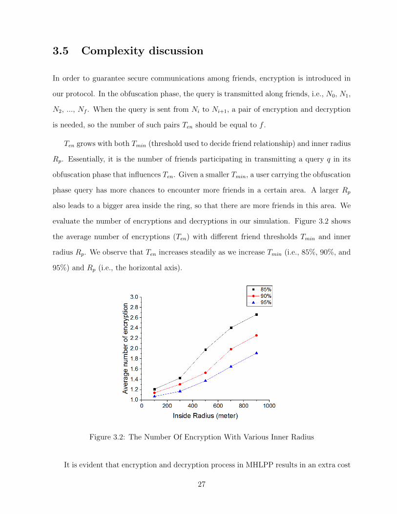
evaluate the number of encryptions and decryptions in our simulation. Figure 3.2 shows
the average number of encryptions (Ten) with different friend thresholds Tmin and inner
radius Rp. We observe that Ten increases steadily as we increase Tmin (i.e., 85%, 90%, and
95%) and Rp (i.e., the horizontal axis).
Figure 3.2: The Number Of Encryption With Various Inner Radius
It is evident that encryption and decryption process in MHLPP results in an extra cost
27

in both energy and computational resources. However, the number of encryptions and
decryptions is quite low (below 3) which reasonable based on the experiment.
3.6 Performance Analysis
We use the map of Helsinki in our simulator to evaluate MHLPP. It is also compared
against the known protocol, Hybrid and Social-aware Location-Privacy in Opportunistic
mobile social networks (HSLPO). The simulation parameters are shown in Table 3.2. All
pedestrians and cars are users in MHLPP. These users are moving on the map along streets
continuously. There is an LBSP fixed at a random location on the map. For each user,
we give him random social values between 0% and 100%, each corresponding to all other
users. Each value has the same probability, so we can compute the expected number of
friends of a user. For example, if we are given a privacy threshold (Tmin) of 85%, then
there might be 15% (100%-85%) users who are friends of a certain user.
As shown in Table 3.2, there are 126 users in the map, just like what authors of SLPD
did. For each of them, say user i, we give him 126 random SV values, which denotes
the relationship strength between him and other users, so that there are 1262 SV s in our
simulation. The SV s are between 0 and 100. As a result, if the Tmin is equal to 85, the
average number of friends of each user should be 18.9 (=126× (100− 85)/100).
Table 3.2: MHLPP Experiment ParametersParameter ValueSimulation Time 10 minutesMap Size (W x H) 4500 m x 3400 mTotal number of users 126Pedestrians/ Cars 84/42Communication Area Radius 10m – 90 mPedestrian Speed 1.8-5.4 Km/hCar Speed 10-50 Km/h
Users are placed at random locations at the beginning of each experiment. We choose
28

another random point for each user, so that he can move back and forth along streets
between that point and the point his starts at. The user speed depends on the user’s type
(pedestrians or cars) and is set randomly. All queries have a 10-minute timeout. The
queries which are expired before they reach the LBSP (the destination) are considered to
be failed in our success ratio statistics.
In the following experiments, we select 100 users randomly each time, and each selected
user sends a query to the destination so that there are 100 queries sent to the destination.
We count the number of queries received by the destination in 20 minutes and calculate
the query success ratio. If LBS receives 75 queries, then the query success ratio is 75%.
One group of parameters (e.g., the communication range, the privacy threshold, and k) is
in correspondence to one scenario and we process 100 times of trials for each scenario. The
experiment result of each scenario we show comes from the average of its corresponding
100 trials.
Figures 3.3-3.5 compare performances between HSLPO and MHLPP for different values
of k, communication radius and privacy threshold (Tmin in MHLPP). The k is the privacy-
level requirement in HSLPO. Both HSLPO and MHLPP have different criteria in which a
query can switch to the free phase. To make them comparable, we create a new parameter,
called obfuscation distance. If a query leaves N0 at location La and switches to the free
phase at Nf whose location is Lb, then the obfuscation distance is the straight-line distance
between La and Lb. We test the obfuscation distances of HSLPO with different parameters,
and then we set the inner radius of MHLPP to those values. The query success ratio is
the ratio of delivered queries to the total number of queries. The number of hops (h)
is the number of intermediate users between N0 and the destination (LBSP). We count
the number of users surrounding the last friend in a specific range, which is k times the
communication radius. We calculate the entropy using the reciprocal of the number of
surrounding users.
29

3.6.1 Query success ratio
The query success ratio is the percentage of delivered queries among a number of attempts.
Based on the timeout value in Table 3.2, a query is delivered successfully, if it arrives at
the LBSP (the destination) before the timeout; otherwise it fails. We use the query success
ratio to evaluate the delivery performance of MHLPP.
30

(a) Query Success Ratio Versus Various k
(b) Query Success Ratio Versus Various Commu-nication Radius
(c) Query Success Ratio Versus Various PrivacyThresholds
Figure 3.3: The Query Success Ratio Comparison Between HSLPO and MHLPP
31

As shown in Figure 3.3(a), the success ratio in MHLPP is always higher than that in
HSLPO. As the value of k increases, HSLPO success ratio drops sharply while MHLPP
remains stable. This is because the larger k is, the harder it is for HSLPO to find enough
friends in a limited time. The lack of friends has less impact on MHLPP. We observe that
the success ratio of MHLPP rises when k = 7. That is because it depends on the inner
radius which is equal to the obfuscation distance of HSLPO. The obfuscation distance
decreases when k = 7, because most of the queries which complete their obfuscation phase
have a short obfuscation distance. In Figure 3.3(b), both HSLPO and MSLPP values
increase and have the same trend when given a larger communication radius. The reason
is that the communication radius effects the free phase more than the obfuscation phase
for both. As shown in Figure 3.3(c), higher privacy threshold leads to lower success ratio in
two algorithms. Its impact on HSLPO is more intense than that on MHLPP, which is the
most important characteristic of MHLPP. MHLPP has a better performance than HSLPO
especially when there are fewer friends in the network. MHLPP can transmit messages
with the help from strangers in its obfuscation phase while HSLPO cannot.
3.6.2 Number of Hops
We count the number of hops it takes for queries to be delivered successfully and calculate
the average. Every user who takes part in the delivery process is considered in the hop
count. We introduce this criterion to measure the routing path length of the algorithm.
MHLPP is more sensitive to the probability that a user encounters a friend than HSLPO
is. The reason is that MHLPP aims to reach a certain distance rather than taking certain
number of hops. In other words, MHLPP continues sending queries to other friends until
queries enter their obfuscation area. In this process, MHLPP takes every chance to forward
queries. If it is hard for MHLPP to find friends, it can also take the queries to obfuscation
areas with fewer friends. Therefore, the probability that users encounter friends has less
impact on the performance of MHLPP. The result is shown in Figure 3.4.
32
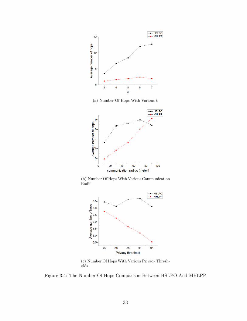
(a) Number Of Hops With Various k
(b) Number Of HopsWith Various CommunicationRadii
(c) Number Of Hops With Various Privacy Thresh-olds
Figure 3.4: The Number Of Hops Comparison Between HSLPO And MHLPP
33

In Figure 3.4(a), the number of hops in HSLPO is affected by parameter k obviously.
Especially, the first k hops forwarders must be friends, which makes it hard for HSLPO to
have queries to be forwarded successfully. Both protocols have similar number of hops in
their free phases, but HSLPO has exactly k hops in its obfuscation phase, while MHLPP
can have fewer than k hops. In figure 3.4(b), the number of hops in MHLPP grows with
the communication radius obviously, while it does not change a lot in HSLPO, because
only successful delivery queries are counted in the statistics. Given a large communication
radius, MHLPP has a much higher success ratio for delivered queries as it can connect
more friends. In Figure 3.4(c), the value of MHLPP drops for higher privacy thresholds.
The reason is the same as Figure 3.4(b). For HSLPO, no matter how hard it is to find
a friend, it attempts to find exactly k friends. However, if it is too hard to find a friend,
MHLPP’s friend can carry the query while moving and complete the obfuscation process.
For higher privacy thresholds (i.e., resulting in fewer friends), MHLPP chooses to carry
queries other than finding friends. That results in a drop in the number of hops.
3.6.3 Security
Since the principles with that two protocols protect original requesters are different, we
evaluate the probability that attackers locate the original requester if the distance between
him and the last friend is smaller than a some value r, which is equal to k times the
communication radius. Since the last friend reveals himself to the LBSP, attackers might
locate him accurately. We assume that attackers know the privacy parameter k. In the
worst case, the distance between the original requester and the last friend is smaller than
r when attackers start to locate the original requester. That gives attackers a chance to
locate the original requester. We count all users who are inside the radius r of the last
friend, and the original requester is one of them. For example, if there are m users in the
area, the probability should be 1m
. Figure 3.5 compares the entropy E of both HSLPO and
34

MHLPP. We use the following formula for computing entropy:
E = − 1
mlog2
(1
m
)(3.5)
From Figure 3.5(a), we observe that MHLPP has very small (about 0.04) increase in
entropy compared to HSLPO. When the original requester is in the circle centered at the
last friend, HSLPO is a little more secure than MHLPP but not by very much. That
is because HSLPO always switches to the free phase when the last friend encounters the
previous friend, so the previous friend must in the circle. MHLPP does not have this
condition. Both graphs in Figure 3.5(a) and Figure 3.5(b) have the same trend. The curve
of MHLPP is also a little higher than that of HSLPO, while two curves almost meet when
the communication radius is small or large. Given a small radius, the entropy of both
protocols are small. When the radius is large, we can ignore the effect of the previous
friend mentioned about for Figure 3.5(a) as there are so many users in the circle. From
Figure 3.5(c), since the circle neither expands or shrinks, we observe that the two curves
exhibit similar behavior. The values of HSLPO are always lower than the correlated values
of MHLPP. However, as we observed in the experiment, the last friend is always hundreds
of meters away from the requester.
35

(a) Locating Probability Entropy With Various k
(b) Locating Probability Entropy With VariousCommunication Radii
(c) Locating Probability Entropy With VariousPrivacy Thresholds
Figure 3.5: Locating Probability Entropy Comparison Between HSLPO And MHLPSP
36

Chapter 4
Appointment Card Protocol
4.1 System Model
The network architecture consists of two main classes of entities: Users and Location-
Based Service Providers (LBSPs). Users are mobile and communicate with other users
and LBSPs within a certain range, i.e., the communication range of their portable devices.
For a given user, other users in the social network are either strangers or his friends whom
he can detect when they are in his communication range. Let RSi,j denote the relationship
strength between user i and j. If RSi,j is larger than a specific threshold, FTmin, user j
is considered a friend of i. LBSPs, which provide location-based services to the users are
fixed and not part of the social network. We assume that the only information which is
necessary for the LBSP is a location from the original requester, but the original requester
should still give an identity (not his own) to the LBSP so that the LBSP can reply to that
identity.
We consider external attacker capable of eavesdropping on limited traffic in the net-
work. We assume that the attacker can access the database of LBSPs, so that he can learn
everything recorded in LBSP’s memory, including user identities and locations. The at-
tacker launches an inference attack on each user who uses the LBS in an attempt to learn
37
user’s private information based on location and context in the queries. Therefore, the
key to protecting location-privacy is degrading the relationship between the user identity
and the location provided by him so that the attacker can hardly infer the identity of the
original requester by the known information.
We propose a protocol, called Appointment Card Protocol (ACP), to protect the
identity and location-privacy of the original requester by providing other users’ identity
(agents), which can be any user in the network so that ACP can have a large anonymity
set. The friends of the original requester separate the agents and the original requester so
that the agents have no knowledge about the original requester.
4.2 Appointment Card Protocol Overview
Our proposed ACP protects original requesters when they are served by LBSPs. Every
user generates Appointment Cards (ACs) containing his own identity called Cid and a
unique number Capt which is generated by himself, and he is the first agent (Agt1) of ACs
generated by himself. The ACs are exchanged when two users encounter each other. The
user who gets the ACs from Agt1 becomes the second agent (Agt2) of the ACs. More users
become the ACs’ agents when they get the ACs, and each AC must have k agents before
a user can use it in a query. When the original requester sends a query, he chooses an AC
and sends the query using the identity Agt1 which is in the AC. The LBSP replies to Agt1
when it receives the query. Agt1 then forwards the reply to the next agent (i.e., Agt2),
and so on until the reply reaches the last agent (Agtk). Agtk is responsible for forwarding
it to the original requester. Therefore, we can consider the ACP having two parts: 1)
users generate and exchange ACs continuously; 2) users use ACs when they want to send
a query.
38

Figure 4.1: Example of ACP Message Exchange
Figure 4.1 is an example of the execution of the ACP protocol. Explanations of the
symbols in the figure are shown in Table 4.1. These symbols and the figure are used
throughout the chapter to help us describe the protocol. For simplicity, we will omit some
superscripts and subscripts from these symbols in the following sections when there is no
ambiguity. The whole process can be considered as the following parts: 1) exchanging
cards among all users who are called agents (i.e., 1 and 2), 2) exchanging cards among
friends (i.e., 3), 3) sending the query using information of ACs (i.e., 4), 4) forwarding the
reply among agents (i.e., 5, 6 and 7), and 5) relaying to the original requester (i.e., 8).
39

Table 4.1: ACP Symbols
Parameter Meanings
Uε An user whose identity is ε.
ACβα The βth appointment card generated by user α.
ACβα,γ ACβ
α is being forwarded by user γ who is an agent.
Queryα(β)δ A query whose original requester is δ and using ACβ
α
Replyα(β) The reply of a query which uses ACβα.
Replyα(β)γ Replyα(β) is being forwarded by user γ who is an agent.
Agtα(β)i The ith (i ≥ 1) agent of ACβ
α.
captβα The parameter Capt in ACβα. see Table 4.2
aaptα(β)γ The parameter Aapt in ACβ
α, which is given by user γ who is anagent. see Table 4.2
AN Both the Capt and the Aapt in an AC are called the AppointmentNumber.
NRε The number of ready-ACs carried by Uε
40

4.3 Appointment Card
To protect the original requester’s location privacy, the original requester uses others’
identity (i.e., Agt1) to send queries to the LBSP instead of his own identity, so that the
LBSP can reply to the original requester through Agt1. ACs make it possible for the agents
to forward the reply to the original requester. In other words, An AC indicates a path
through which the original requester can get his reply.
In Figure 4.1, Ua, Ub, and Uc are the agents of ACβa (i.e., Agt
a(β)1 , Agt
a(β)2 and Agt
a(β)3 ).
These agents are strangers, so the attackers can hardly infer Uc from the identity of Ua.
At the same time, Uc is in the original requester Ud’s social tie (i.e.,Uc is Ud’s friend or his
friends’ friend, so on), and he is the only one who knows how to reach Ud. Therefore, it is
hard for attackers to infer the identity of Ud from the identity of Ua.
Notice that Uc receives ACβa from a stranger Ub who knows the information of ACβ
a and
the identity of the next agent Uc, so that it is unsafe for Uc to use ACβa . In other words,
ACβa cannot be used until Uc gives it to another user (e.g., the user d) who trusts Uc. The
AC is called a ready appointment card (simply ready-AC) after it leaves the last agent (i.e.,
Uc), or it is called the distributing appointment card (simply distributing-AC). It is obvious
that distributing-ACs are transmitted among agents who can be strangers, while an user
can only get ready-ACs from one of his friends.
To make users carry a similar number of ready-ACs, ready-ACs are also exchanged
between friends, so that an user can get ready-ACs from his friends who have more ready-
ACs than him. As a result, the last agent is not sure whether the user who gets the
ready-AC from him is the original requester. We introduce a pseudonym mechanism which
enables the last agent to forward the reply to the unknown original requester.
All users in the network are responsible for generating their respective ACs, and they
are called the creators of their own ACs. The creator records his own identity (Cid) and a
unique number (Capt) on his AC. When users exchange ACs, they modify Aid (the agent
41

ID) and Aapt (the agent’s appointment number) in the AC to enable the next agent to
identify who is the predecessor. Entries of ACs are shown in Table 4.2.
Table 4.2: Appointment Card
Parameter Meanings
Cid The identity of the creator who generates the AC.
Capt A unique number that distinguishes an AC from otherones generated by the same creator.
Aid The identity of an agent who gives the AC to the recentholder. (The previous hop of the AC)
Aapt A unique number that distinguishes an AC from otherones transmitted by the same agent.
Timeout The time when the AC expires.
EQ A queue (Exchange Queue) which records the AC’sagents in order. Its length is EQL.
4.4 AC Life Cycle
The life cycle of an AC starts when it is generated by its creator. The first k (see Table 4.3)
agents add their identities into its Exchange Queue (EQ) (see Table 4.2) before exchanging
it, which increases the length (EQL) of the EQ. When the AC’s EQL reaches k, it is eligible
to be used in a query and is called a ready-AC. When an AC is used in a query, it is marked
as an used AC by the original requester who uses the AC. An AC starts at the distributing
state. No matter what state (distributing, ready or used) an AC is in, it can expire, as
shown in Figure 4.2. If the length of its EQ reaches k, it is switched to the ready state.
When an user uses a ready-AC in a query, the AC is switched to the used state. The user
can also use the used -AC in other queries but he does not give the used -AC to anyone else.
42

Figure 4.2: AC’s Life Cycle
4.5 System Parameters
All the system parameters are shown in Table 4.3.
Table 4.3: Important System Parameters
Parameter Meanings
k The obfuscation distance
m The friend obfuscation distance
GP The generating period of ACs
Seg The distributing segment
τ Avoiding time
AT The timeout for ACs
4.5.1 Obfuscation Distance
The obfuscation distance k is the number of exchange before an AC is switched to the ready
state. In other words, an AC must be exchanged k times before it becomes a ready-AC
which can be used by an user in queries.
As shown in Figure 4.3, the k agents are strangers so that the only relationship between
two adjacent ones is that they encounter each other somewhere. The relationship between
Agt1 and Agtk becomes weaker when we increase k. In other words, attackers can hardly
43

infer the identity of Agtk when they only know the identity of Agt1, and the difficulty
increases with the increase of parameter k. As a result, it is hard for attackers to infer
the identity of the original requester, even though Agtk is in the social tie of the original
requester. Since the reply message must go through a series of agents, a long obfuscation
distance also lengthens the path of the reply message. Therefore, a large k makes the
original requester safer, while making it harder and longer for the reply to be delivered.
Figure 4.3: Obfuscation Distance
4.5.2 Friends Obfuscation Distance
Since Agtk−1 is a stranger for Agtk, it is possible that Agtk−1 is the attacker. We assume
that the attacker knows that Agtk is in the social tie of the original requester. The attacker
can assume that Agtk is a close friend of the original requester, so the identity of Agtk
gives the attacker a good tip to infer the original requester. A solution to prevent the
agent Agtk−1 from learning the identity of the original requester easily is that the last
m (1 ≤ m ≤ k) agents are friends, as shown in Figure 4.4. Here, m is called friends
obfuscation distance, and the last m agents are trusted agents.
It is true that Agti is a friend of Agti+1, i > k−m, but two nonadjacent trusted agents
(e.g., Agti and Agti+2) might have a weak relationship. Since there are at least m trusted
agents between the stranger Agtk−m and the original requester, Agtk−m can hardly infer
the identity of the original requester based on information he learns. When m = k, all
ACs must be exchanged between friends only. When m = 1, the last agent is the only one
44

Figure 4.4: Friends-Obfuscation Distance
who is in social tie of the original requester, which is the case in our example.
However, friends encounter each other rarely, so having a large m increases the difficulty
of distributing ACs. In this work, we assign m to 1.
4.5.3 Generating Period
Since ACs could expire, users must generate new ACs continuously. We use GP to denote
the speed of generating new ACs per user; that is, each user generates a new AC every GP
seconds.
4.5.4 Distributing Segment
It is the series of random agents that increases the difficulty for attackers to infer the
identity of the original requester. However, it is possible that many ACs are transmitted
by the same series of agents. We use the system parameter distributing segment, Seg,
to avoid giving all distributing-ACs to the same user. Each user maintains Seg number
of Distributing AC Lists (DLs) and puts received distributing-ACs in one of those DLs
randomly. If Agti exchanges ACs with another user, Agti selects one of his DLs, and only
ACs in that DL will be given to that user.
In our example Figure 4.1, we assume that Seg is equal to two so that each user has
two DLs (i.e., DL1 and DL2). When Ub receives AC1a,a, AC
2a,a and AC3
a,a from Ua, Ub may
45

put AC1a,a and AC2
a,a in its DL1, while AC3a,a in its DL2. If Ub encounters Uc, Ub can give
either AC1a,b and AC2
a,b or only AC3a,b to Uc. In this way, we separate the ACs generated
by the same creator Ua.
4.5.5 Avoiding Time
It makes the obfuscation path of an AC simpler that the AC has duplicate agents, which
facilitate attackers’ inference about the identity of the original requester. We use a pa-
rameter avoiding time, τ , to optimize the agent selection strategy. If an user gets an
distributing-AC at time ti, he cannot get that distributing-AC again before time ti + τ .
For example, we assume that two users, e.g., UA and UB, are walking together for a
period. Also assume that UA generates an AC (e.g., ACA) at t0 and gives it to UB, then
ACA is given back to A and so on. The distributing phase of the AC only costs a few
seconds, because UA and UB exchange ACA time and again, but they are the only agents
involved. The above scenario defeats the purpose of exchanging ACs because it is easy
for an attacker to infer the identity of the last agent (UA or UB) from the first agent UA.
We can prevent an AC from having duplicate agents when using the parameter τ . For
example, UB receives a certain AC ACA from UA at t0, then UB sends it to an user C
(UC) who can also send it to others. If an user carrying ACA encounters UB before t0 + τ ,
he cannot send ACA to UB. Therefore, if the parameter τ is larger than or equal to the
parameter AT, there is no duplicate agent in an AC’s EQ. In other words, an AC never
reaches an agent twice when τ is equal to AT. In this thesis, we assign τ to AT.
4.5.6 AC Timeout
Let AT denote the timeout of ACs. An AC expires AT seconds after it is generated. When
an AC expires, all agents delete the AC information from their memory.
46

4.6 Protocol Details
4.6.1 Generating ACs
Maintaining a certain number of ACs in the network is a prerequisite for users for sending
queries. Considering that ACs can expire, users must generate ACs continuously. The user
who generates an AC is called the creator of the AC; at the same time, he is also the first
agent of the AC. ACs are created based on two principles: fairness and continuity.
ACs impose a burden on agents. In fact, agents are unlikely to benefit from relaying
messages to the original requester because they need to allocate memory to save ACs’
information and consume energy to forward replies. To prevent users who generate more
ACs than others from being overloaded, some fairness mechanism must be in place to
ensure that all users generate a relatively equal number of ACs.
We assume that AT is equal to 30 minutes, and every user generates 100 ACs at
the beginning and generates no AC until the 30th minute. Since all agents remove the
information of expired ACs from their memory, they can hardly deliver replies which use
expired ACs. As a result, it is hard for an user to select an appropriate AC for his query
at the 29th minute when all ACs only have 1 (= 30 − 29) more minute, because agents
may not be able to forward the reply of his query even though the LBS receives the query
successfully. Therefore, the generating strategy should be steady and sustainable.
In our protocol, each user generates a new AC every GP second. Since an AC has an
AT -seconds timeout, there are δ = ATGP
ACs held by each user in the network. In other
words, each user maintains about δ ACs which is generated by himself, and we meet the
fairness criteria. Since users create ACs continuously, ACs have various timeouts so that
it is likely for an user to pick an AC which does not expire in a long time (at least longer
than his queries and replies).
47

4.6.2 Exchange Distributing Appointment Cards
Users exchange their distributing-ACs as frequently as possible, so that a distributing-AC
can be switched to a ready one quickly. Still, there are some other conditions which should
be satisfied when exchanging a distributing-AC. Users should avoid giving all their ready-
ACs to a single user, which leads to identical set of AC agents. As shown in subsection
4.5.4, we use Seg and DLs to separate distributing-ACs. We also need to prevent ACs from
having duplicate agents using τ which is described in subsection 4.5.5.
Now we propose the strategy of exchanging distributing-ACs. Let us take a pair of
users Alice and Bob as an example. If Alice encounters another user Bob, Bob tells Alice
whether he trusts her (Bob views her as a friend). Alice picks one of her distributing-AC
lists (e.g., DL1). Alice traverses all ACs in DL1, and distributing-ACs which satisfy the
following two conditions should be given to Bob:
1. If the AC’s EQL is not shorter than k −m, then Alice must be a friend of Bob.
2. Bob was not carrying the AC in the recent τ time interval.
When Alice sends a distributing-AC to Bob, she adds her identity and the current time
to the AC’s EQ. Besides, Alice must modify the AC’s Aid to her own identity and its Aapt
to a new random number. She also records the information in Table 4.4 as relay-table in
her memory. We should notice that the first agent (i.e., the creator) does not have the
Aaptold and the Aidold, because he is precisely the one who has generated the AC. In that
case the Aaptold and the Aidold indicate the Capt he gives to the AC and his own identity.
When Bob gets those ACs, he puts each one of the received distributing-ACs in his DLs
respectively and randomly. If an AC whose EQL is already equal to k, the AC must be
switched to a ready state when Bob gets it. Bob puts ready-ACs in his ready-AC list
instead of distributing-AC lists.
48

Table 4.4: Relay Table Entries
Parameter Meanings
Aaptold The Aapt generated by the previous agent
Aidold The identity of the previous agent
Aaptnew The new Aapt (generated by himself)
IDnxt The identity of the next agent
EQL The AC’s EQL (should larger than 0)
AT The time when the AC times out.
4.6.3 Exchange Ready Appointment Cards
Users ask for ready-ACs only from their friends, which prevents strangers from learning
the information of the users who are holding the ready-ACs. The strategy of exchanging
ready-ACs should also meet some fairness criteria. That is, the number of each user’s
ready-ACs should be more or less equal.
Let us consider two friends Alice and Bob as an example. Alice has 20 ACs, while Bob
has 10 ACs. When they encounter each other, it is reasonable that they both give half of
their ready-ACs to each other. As a result, they both will have half of the total (20+102
)
ACs. However, that strategy does not work in the following condition. Alice is a friend of
Bob, while Bob is not a friend of Alice. In other words, Bob trusts Alice, but Alice does not
trust Bob. We assume that Alice is a trusted but suspicious girl so that many users trust
her while she trusts few users while Bob is opposite. When users encounter Alice, they
ask for ready-ACs from her, but Alice rarely asks for ready-ACs. Therefore, Alice carries
few ready-ACs, while Bob carries many ready-ACs. When Alice and Bob encounter each
other, and Bob asks for ready-ACs, then the strategy seems unfair for Alice. To ensure
the fairness and the efficiency of the strategy, users must compare the number of their
own ready-ACs and the number of ready-ACs carried by the other user when two users are
exchanging ready-ACs.
49

When Bob encounters Alice, Bob tells Alice the number of his ready-ACs (NRBob)
and whether he wants Alice’s ready-ACs (if he trusts Alice). If Alice learns that Bob
needs her ready-ACs, she compares the number of her ready-ACs (NRAlice) and NRBob. If
NRBob ≥ NRAlice, Alice gives no ready-AC to Bob; otherwise, she gives NRAlice−NRBob
2to
Bob. In this way, ready-ACs do not concentrate in a group of users who trust many users.
The process of exchanging ready-ACs is much more straightforward than that for dis-
tributing-ACs. Users do not modify any information in the ready-ACs including Aapt and
Aid so that the parameters of ready-ACs always stay the same.
The algorithm of exchanging ACs when an user Ui encounters another user Uj is shown
in Algorithm 4.1. The two users tell each other whether they are friends at the very
beginning of their encounter. After they both know their relationship, they start to ex-
change their distributing-ACs. When they both finish receiving the distributing-ACs from
the other, they continue to exchange their ready-ACs at the same time. The process ends
when they finish exchanging their ready-ACs (or they do not need to exchange ready-ACs).
4.6.4 Sending Queries
The original requester must be able to send his queries to the LBSP and be able to get the
reply while preventing the LBSP from learning his identity. In ACP, the original requester
sends his query using Agt1’s identity to the LBSP, and Agt1 is responsible for forwarding
the reply from LBSP to the original requester. Therefore, the original requester’s query
includes a sender identity Agt1, which is equal to the Cid in the AC. Since Agt1 needs a
Capt to identify the AC used by the query (and the reply), the Capt in the AC is also in
the query. The network can deliver that query to the destination LBSP efficiently with
any DTN protocol.
We use the example in Figure 4.1. The original requester Ud has an AC (i.e., ACβa,c)
whose creator is Ua. When Ud uses ACβa,c to send his query Query
a(β)d , the sender identity
50

Algorithm 4.1 Algorithm for exchanging ACs
1: procedure Encounter(Uj)2: if Ui trusts Uj then3: Ui tells Uj that Uj is viewed as a friend.4: else5: Ui tells Uj that Uj is not viewed as a friend.6: end if7: Wait for Uj to tell Ui whether Ui is viewed as a friend.8: Ui chooses a distributing list (DLω) randomly.9: for each ACu in DLω do10: if Uj was carrying ACu in the recent τ time then11: ACu cannot be sent to Uj12: continue (Try the next one.)13: end if14: if the EQL of ACu ≥ k −m then15: if Ui is not trusted by Uj then16: ACu cannot be sent to Uj17: continue (Try the next one.)18: end if19: end if20: Send ACu to Uj21: end for22: Tell Uj that all distributing-ACs are sent.23: Receive all distributing-ACs from Uj24: if Ui trusts Uj then25: Ui tells Uj NRi.26: end if27: if Ui is trusted by Uj then28: Wait for Uj to tell Ui NRj.29: if NRj ≥ NRi then30: send no ready-AC to Uj31: else32: send
NRi−NRj
2number of ready-ACs to Uj
33: end if34: Tell Uj all ready-ACs are sent.35: end if36: if Ui trusts Uj then37: Wait for ready-ACs from Uj.38: end if39: end procedure
51

is a, and the Capt of the query is the captβa , as shown in Figure 4.5.
Figure 4.5: Constitute Query
The AC is marked as used when the query is ready to be sent so that the AC cannot
be given to other users. The original requester also uses a pseudonym to receive the reply,
which is described in subsection 4.6.5.4. The algorithm that an user Ui uses to send a
query is shown in Algorithm 4.2.
Algorithm 4.2 Algorithm for Sending Queries
1: procedure SendQuery2: Choose an ready-AC or used -AC, say ACβ
α,f .3: if The AC is in the ready state then4: Switch the AC to the used state.5: end if6: Assign the sender identity of the query to Uα7: Assign the receiver identity to the LBS8: Assign the AN to the captβα9: Get a pseudonym pseudo
(Uf , aapt
α(β)f
)10: Use the pseudonym as Ui’s identity.11: Send the query to the LBS.12: end procedure
4.6.5 Sending Replies
4.6.5.1 The LBSP part
When the LBSP receives the query, it learns that the sender’s identity is the first agent
Ua instead of the original requester Ud, which protects the location privacy of the original
52

requester. In Figure 4.6, the LBS provider replies to the sender Ua, when it receives
Querya(β)d . The reply also includes the Capt of the query (i.e., captβa), which enables Ua to
identify the AC used in the query and the reply.
Figure 4.6: Constitute Replies
4.6.5.2 The First Agent
When the first agent (i.e., Agt1) gets the reply from the LBSP, he learns the AN in the
reply. He searches his reply-table to get the information of the AC used in the query and
reply. If the AC does not expire, there must be a corresponding entry in his reply-table. As
shown in Table 4.5, it should be an entry where the Aidold and Aaptold are equal to Agt1’s
identity and the AN of the reply, respectively. As a result, Agt1 learns the identity of the
next agent (i.e., Agt2) from the IDnxt of the entry, so Agt1 forwards the reply to Agt2.
The AN of the reply is replaced with the Aaptnew in the entry by Agt1, which enables Agt2
to identify the AC in Agt2’s reply-table.
Table 4.5: Reply Table Entries of The First Agent
Name of Entries Value
Aidold The user’s own identity
Aaptold The Capt of the AC used in the reply (query)
IDnxt The identity of the second agent
Aaptnew The Aapt given to the second agent by the user.
EQL 1
AT The time when the AC times out.
53

For the example in Figure 4.1, the first agent is Ua. When he receives Replya(β)LBS, he
learns that it is a reply from the LBS and the Capt of the AC is captβa . He searches his
reply-table for an entry whose Aidold is equal to a and Aaptold is equal to captβa . As shown
in Figure 4.7, the IDnxt in the entry is equal to b so he modifies the receiver of the reply
message to Ub. Ua also modifies the AN in the reply message to aapta(β)a which is exactly
equal to the Aaptnew in his reply-table entry, which enables Ub identifies the AC in his
reply-table.
Figure 4.7: The Reply of The First Agent
4.6.5.3 Intermediate Agents
The process of forwarding replies in the intermediate agents (the second to the (k − 1)th
one) is similar to that of the first agent. We take the second agent as an example. When the
second agent receives the reply forwarded by the first one, he learns the sender’s identity
(i.e., the first agent) and the AN from the reply. In his reply-table shown in Table 4.6,
the corresponding entry for the AC used in the reply have Aidold of Agt1 and Aaptold of
Aapt given by Agt1, because he gets the AC from the first agent. More specifically, his
reply-table must include an entry whose Aidold is equal to the previous agent’s identity and
the Aaptold is the value of AN in the received reply.
For the example in Figure 4.1, the second agent is Ub. When he receives Replya(β)a , he
learns that it is Ua who forwards the reply message Replya(β)a and the Aapt of the AC is
aapta(β)a . He searches his reply-table for an entry whose Aidold is equal to a and Aaptold
54
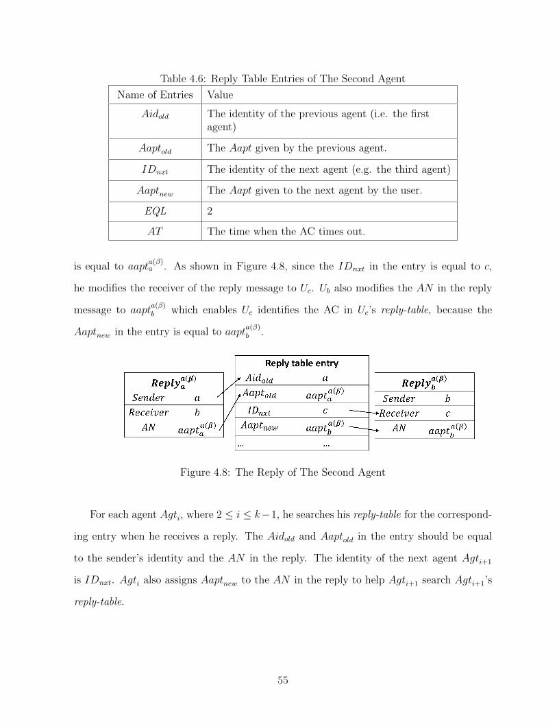
Table 4.6: Reply Table Entries of The Second Agent
Name of Entries Value
Aidold The identity of the previous agent (i.e. the firstagent)
Aaptold The Aapt given by the previous agent.
IDnxt The identity of the next agent (e.g. the third agent)
Aaptnew The Aapt given to the next agent by the user.
EQL 2
AT The time when the AC times out.
is equal to aapta(β)a . As shown in Figure 4.8, since the IDnxt in the entry is equal to c,
he modifies the receiver of the reply message to Uc. Ub also modifies the AN in the reply
message to aapta(β)b which enables Uc identifies the AC in Uc’s reply-table, because the
Aaptnew in the entry is equal to aapta(β)b .
Figure 4.8: The Reply of The Second Agent
For each agent Agti, where 2 ≤ i ≤ k−1, he searches his reply-table for the correspond-
ing entry when he receives a reply. The Aidold and Aaptold in the entry should be equal
to the sender’s identity and the AN in the reply. The identity of the next agent Agti+1
is IDnxt. Agti also assigns Aaptnew to the AN in the reply to help Agti+1 search Agti+1’s
reply-table.
55

4.6.5.4 The Last Agent
The last agent also searches for a reply-table entry based on the reply, while he cannot get
the identity of the next agent. The reply-table entry of the last agent is shown in Table
4.7.
Table 4.7: Reply Table Entries of The Last Agent
Name of Entries Value
Aidold The identity of the previous agent (i.e., the secondagent)
Aaptold The Aapt given by the previous agent.
IDnxt VOID
Aaptnew The Aapt given to the original requester.
EQL k
AT The time when the AC times out.
The last agent uses the same way to look the entry up in his reply-table based on the
reply. When he finds that the EQL is equal to k, he notices that he is the last agent. Then,
he is responsible for forwarding the reply to the original requester instead of forwarding
to another agent. He uses his identity and Aaptnew in his reply-table entry to generates a
pseudonym as follows:
psda(β)Agtk
= pseudo (Agtk, Aaptnew) (4.1)
where the function pseudo (id, Aapt) is a public pseudonym generating function which
everyone in the network knows, including the original requester.
When the original requester sends his query, he also gets the same pseudonym psda(β)Agtk
using the pseudonym generating function. Note that he can get parameters from the AC.
Agtk and Aaptnew are equal to the Aid and Aapt in the AC. He uses that pseudonym as
his identity before he gets the reply.
56

When users deliver the reply from the last agent, they are looking for an user whose
identity is that pseudonym. At last, the original requester gets the reply, because he is the
only user who uses the pseudonym as his identity.
For the example in Figure 4.1, the last agent is Uc. When he receives Replya(β)b , he
learns that it is Ub who forwards the reply message Replya(β)b and the Aapt of the AC is
aapta(β)b . He searches his reply-table for an entry whose Aidold is equal to b and Aaptold is
equal to aapta(β)b . Since the EQL in the entry is equal to 3 (i.e. k), he recognizes that he
is the last agent. Uc calculates the pseudonym psda(β)c = pseudo(c, aapt
a(β)c
)then forward
the reply to psda(β)c . The original requester Ud gets the identity c and the aapta(β)c from
the AC he uses, so that he uses the pseudonym psda(β)c as his identity. As a result, Ud
get the reply from Uc. The AN of the reply is also assigned to aapta(β)c to avoid identical
pseudonyms. The process is shown in Figure 4.9.
Figure 4.9: The Reply of the Last Agent
The algorithm of forwarding replies when an agent Ui gets a reply message from Uprev
is shown in Algorithm 4.3. Ui learns the AN and the identity of the sender from the reply
message Replyα(β)Uprev
. Based on this information, Ui checks his reply-table to find out where
the reply should be forwarded to, which is IDnxt. After Ui updates the AN of the reply
message, he forwards the reply message to IDnxt.
57

Algorithm 4.3 Algorithm For Forwarding Replies
1: procedure Received(Replyα(β)Uprev
)
2: Get the AN from Replyα(β)Uprev
3: if Uprev is the LBS then
4: search Ui’s relay-table to find an entry Eα(β)i
5: whose Aaptold = AN and Aidold = Ui6: else7: search Ui’s relay-table to find an entry E
α(β)i
8: whose Aaptold = AN and Aidold = Uprev9: end if10: Get the EQL, Aaptnew and IDnxt from E
α(β)i
11: Assign the AN of Replyα(β)Uprev
to Aaptnew.12: Assign the sender identity to Ui.13: if EQL = k then14: IDnxt ← pseudo (Ui, Aaptnew)15: end if16: Forward the reply to IDnxt
17: end procedure
4.7 Appointment Number
The Appointment Number (AN) including Capt and Aapt is significant information in the
AC. We explain the rules of generating them in detail and talk about the effect of ACs’
timeout mechanism in this section.
4.7.1 Creator Appointment Number
The Creator Appointment Number (Capt) is a number which is used to identify ACs
generated by the same creator. In other words, if two ACs are generated by the same
creator, and they do not expire, their Capt must be different. Therefore, the first agent
(i.e., the creator) cannot find two entries which have the same Aaptold in his reply-table, if
their Aidold are both his own identity.
58

4.7.2 Agent Appointment Number
The Agent appointment number (Aapt) is a number used to identify ACs which have the
same agent. Agents generate a new Aapts for ACs before they exchange those cards to
others. In other words, an agent gives any AC passing on by him a unique Aapt, which
helps the next agent identify the AC in his reply-table. Since the Aapt is unique, an agent
who is not the first one cannot find the replicated pair, Aidold and Aaptold, in his reply-table.
4.7.3 Timeout
Agents delete the entries, which contains the information of expired ACs, from his reply-
table. Consequently, agents cannot forward replies using ACs which expire. That is the
reason why an original requester must choose an AC which expires after his query and
reply time out. However, the timeout mechanism is still necessary for the protocol.
Since users are moving, the distance between agents and the original requester might
be too large after a long time. As a result, it is hard for agents to forward the reply
messages back to the original requester so that the original requester takes a high risk
when he uses an AC which exists for a long time. Then this kind of ACs might not be
used after a period, while it cost agents a few memories to save the ACs’ information in
their reply-table. Therefore, all users remove the information of expired ACs to save their
memories.
We should also notice that an unexpired AC and an expired one might have the same
Capt or Aapt. Because no agent keeps the record of the expired AC, the duplication cannot
confuse agents.
59

4.8 Example
In the following example, we use 5 users (i.e., Alice, Bob, Charlie, David and Elizabeth)
to show the process of ACP. We should notice that David trusts Charlie (Charlie does not
trust David), Elizabeth trusts David (David does not trust Elizabeth). Users do not trust
others except the above two pairs. The parameters are shown in Table 4.8.
Table 4.8: Example Parameters
Parameters Explanation
k 3
m 1
Seg 2
GP 10 minutes
AT 80 minutes
τ 80 minutes (equal to AT )
We abstract the event that users encounter each other in Table 4.9. Let ti denote the
ith minute. The table lists the time when two users encounter each other. For example,
Charlie and Elizabeth encounter each other at the third minute (t3). After two users meet,
they separate in one minute.
We assume that these users do not encounter any user for a long time, so that they
each has 8 (= 80min10min
) ACs generated by themselves. We also assume that no AC expires in
our 8-minutes example. Since the parameter Seg is equal to 2, each user has 2 Distributing
AC Lists (DLs). The initial state of our example is shown in Table 4.10. To make the
example simple and clear, we do not place ACs in DLs randomly, ACs are always placed
in the DL alternately. For example, if we put the first AC in DL1, then the second AC
must be in the DL2. Users also obey the rule when they receive ACs from other users.
The explanation of symbols used in table are shown in the former Table 4.1. To make
the symbol clear, we add the EQL of the AC on the superscript. For example, if the EQL
60

Table 4.9: Example Event
User 1 User 2 Time
Elizabeth Bob t1
Bob Charlie t2
Charlie Elizabeth t3
Elizabeth Alice t4
Bob Charlie t5
Alice Charlie t6
Charlie David t7
David Elizabeth t8
Table 4.10: Example Initial State
User Identity DL1 DL2 RL
Alice (A) AC1[0]A ,AC
3[0]A ,AC
5[0]A ,AC
7[0]A AC
2[0]A ,AC
4[0]A ,AC
6[0]A ,AC
8[0]A ∅
Bob (B) AC1[0]B ,AC
3[0]B ,AC
5[0]B ,AC
7[0]B AC
2[0]B ,AC
4[0]B ,AC
6[0]B ,AC
8[0]B ∅
Charlie (C) AC1[0]C ,AC
3[0]C ,AC
5[0]C ,AC
7[0]C AC
2[0]C ,AC
4[0]C ,AC
6[0]C ,AC
8[0]C ∅
David (D) AC1[0]D ,AC
3[0]D ,AC
5[0]D ,AC
7[0]D AC
2[0]D ,AC
4[0]D ,AC
6[0]D ,AC
8[0]D ∅
Elizabeth (E) AC1[0]E ,AC
3[0]E ,AC
5[0]E ,AC
7[0]E AC
2[0]E ,AC
4[0]E ,AC
6[0]E ,AC
8[0]E ∅
61

of AC1A,X is equal to 2, it is marked as AC
1[2]A,X .
4.8.1 Exchanging Appointment Cards
To make it easier, users do not pick DLs randomly as we described in the previous sections
when they exchange ACs. Instead, If we say that Ux encounters Uy, Ux always picks his
DL1 and Uy always picks his DL2.
The tables in current section show the entire distributing-AC Lists (i.e., DL1 and DL2)
and entire relay-tables (RLs) of each user. We use the initial letter to denote each user in
symbols. For example, D denotes David. The structure of the AC-list tables is shown in
Table 4.11.
Table 4.11: User X and Y’s AC Lists
X
DL1Before X’s distributing-AC list 1 before their exchange.
After X’s distributing-AC list 1 after their exchange.
DL2Before X’s distributing-AC list 2 before their exchange.
After X’s distributing-AC list 2 after their exchange.
RLBefore X’s ready-AC list before their exchange.
After X’s ready-AC list after their exchange.
Y
DL1Before Y’s distributing-AC list 1 before their exchange.
After Y’s distributing-AC list 1 after their exchange.
DL2Before Y’s distributing-AC list 2 before their exchange.
After Y’s distributing-AC list 2 after their exchange.
RLBefore Y’s ready-AC list before their exchange.
After Y’s ready-AC list after their exchange.
The process of exchanging AC is shown step by step as follows.
1. Elizabeth encounters Bob
62

At t1 (the first minute), Elizabeth encounters Bob. Elizabeth picks her DL1, and Bob
picks his DL2. They give distributing-ACs in their picked DLs to each other and update
their reply tables, as shown in Table 4.12 and Table 4.13.
Table 4.12: Elizabeth and Bob’s AC Lists at Time t1
Elizabeth
DL1Before AC
1[0]E ,AC
3[0]E ,AC
5[0]E ,AC
7[0]E
After AC2[1]B,B,AC
6[1]B,B
DL2Before AC
2[0]E ,AC
4[0]E ,AC
6[0]E ,AC
8[0]E
After AC2[0]E ,AC
4[0]E ,AC
6[0]E ,AC
8[0]E ,AC
4[1]B,B,AC
8[1]B,B
RLBefore ∅After ∅
Bob
DL1Before AC
1[0]B ,AC
3[0]B ,AC
5[0]B ,AC
7[0]B
After AC1[0]B ,AC
3[0]B ,AC
5[0]B ,AC
7[0]B ,AC
1[1]E,E,AC
5[1]E,E
DL2Before AC
2[0]B ,AC
4[0]B ,AC
6[0]B ,AC
8[0]B
After AC3[1]E,E,AC
7[1]E,E
RLBefore ∅After ∅
Table 4.13: Elizabeth and Bob’s Relay Table At Time t1Elizabeth Bob
Aidold Aaptold IDnxt Aaptnew EQL Aidold Aaptold IDnxt Aaptnew EQL
E capt1E B aaptE(1)E 1 B capt2B E aapt
B(2)B 1
E capt3E B aaptE(3)E 1 B capt4B E aapt
B(4)B 1
E capt5E B aaptE(5)E 1 B capt6B E aapt
B(6)B 1
E capt7E B aaptE(7)E 1 B capt8B E aapt
B(8)B 1
2. Bob encounters Charlie
At t2 (the second minute), Bob encounters Charlie. Bob picks his DL1, and Charlie
picks his DL2. They give distributing-ACs in their picked DLs to each other and update
their reply tables, as shown in Table 4.14 and Table 4.15.
63

Table 4.14: Bob and Charlie’s AC Lists at Time t2
Bob
DL1Before AC
1[0]B ,AC
3[0]B ,AC
5[0]B ,AC
7[0]B ,AC
1[1]E,E,AC
5[1]E,E
After AC2[1]C,C ,AC
6[1]C,C
DL2Before AC
3[1]E,E,AC
7[1]E,E
After AC3[1]E,E,AC
7[1]E,E,AC
4[1]C,C ,AC
8[1]C,C
RLBefore ∅After ∅
Charlie
DL1Before AC
1[0]C ,AC
3[0]C ,AC
5[0]C ,AC
7[0]C
After AC1[0]C ,AC
3[0]C ,AC
5[0]C ,AC
7[0]C ,AC
1[1]B,B,AC
5[1]B,B,AC
1[2]E,B
DL2Before AC
2[0]C ,AC
4[0]C ,AC
6[0]C ,AC
8[0]C
After AC3[1]B,B,AC
7[1]B,B,AC
5[2]E,B
RLBefore ∅After ∅
Table 4.15: Bob and Charlie’s Relay Table At Time t2Bob Charlie
Aidold Aaptold IDnxt Aaptnew EQL Aidold Aaptold IDnxt Aaptnew EQL
B capt2B E aaptB(2)B 1 C capt2C B aapt
C(2)C 1
B capt4B E aaptB(4)B 1 C capt4C B aapt
C(4)C 1
B capt6B E aaptB(6)B 1 C capt6C B aapt
C(6)C 1
B capt8B E aaptB(8)B 1 C capt8C B aapt
C(8)C 1
B capt1B C aaptB(1)B 1
B capt3B C aaptB(3)B 1
B capt5B C aaptB(5)B 1
B capt7B C aaptB(7)B 1
E aaptE(1)E C aapt
E(1)B 2
E aaptE(5)E C aapt
E(5)B 2
3. Charlie encounters Elizabeth
At time t3, Charlie encounters Elizabeth. Charlie picks his DL1, and Elizabeth picks
her DL2. They give distributing-ACs in their picked DLs to each other and update their
64

reply tables, as shown in Table 4.16 and Table 4.17.
We should notice that Charlie does not give AC1[2]E,B to Elizabeth, because Elizabeth
does not trust Charlie. The EQL of the AC1[2]E,B has already reached 2, which is equal to
k−m = 3− 1. As mentioned in subsection 4.6.2, these kinds of ACs are only sent to users
who trust the current agent. Therefore, Charlie cannot give AC1[2]E,B to Elizabeth when she
does not trust him.
Table 4.16: Charlie and Elizabeth’s AC Lists at Time t3
Charlie
DL1Before AC
1[0]C ,AC
3[0]C ,AC
5[0]C ,AC
7[0]C ,AC
1[1]B,B,AC
5[1]B,B,AC
1[2]E,B
After AC1[2]E,B,AC
2[1]E,E,AC
6[1]E,E,AC
4[2]B,E
DL2Before AC
3[1]B,B,AC
7[1]B,B,AC
5[2]E,B
After AC3[1]B,B,AC
7[1]B,B,AC
5[2]E,B,AC
4[1]E,E,AC
8[1]E,E,AC
8[2]B,E
RLBefore ∅After ∅
Elizabeth
DL1Before AC
2[1]B,B,AC
6[1]B,B
After AC2[1]B,B,AC
6[1]B,B,AC
1[1]C,C ,AC
5[1]C,C ,AC
1[2]B,C
DL2Before AC
2[0]E ,AC
4[0]E ,AC
6[0]E ,AC
8[0]E ,AC
4[1]B,B,AC
8[1]B,B
After AC3[1]C,C ,AC
7[1]C,C ,AC
5[2]B,C
RLBefore ∅After ∅
65

Table 4.17: Charlie and Elizabeth’s Relay Table At Time t3Charlie Elizabeth
Aidold Aaptold IDnxt Aaptnew EQL Aidold Aaptold IDnxt Aaptnew EQL
C capt2C B aaptC(2)C 1 E capt1E B aapt
E(1)E 1
C capt4C B aaptC(4)C 1 E capt3E B aapt
E(3)E 1
C capt6C B aaptC(6)C 1 E capt5E B aapt
E(5)E 1
C capt8C B aaptC(8)C 1 E capt7E B aapt
E(7)E 1
C capt1C E aaptC(1)C 1 E capt2E C aapt
E(2)E 1
C capt3C E aaptC(3)C 1 E capt4E C aapt
E(4)E 1
C capt5C E aaptC(5)C 1 E capt6E C aapt
E(6)E 1
C capt7C E aaptC(7)C 1 E capt8E C aapt
E(8)E 1
B aaptB(1)B E aapt
B(1)C 2 B aapt
B(4)B C aapt
B(4)E 2
B aaptB(5)B E aapt
B(5)C 2 B aapt
B(8)B C aapt
B(8)E 2
4. Elizabeth encounters Alice
At time t4, Elizabeth encounters Alice. Elizabeth picks her DL1, and Alice picks her
DL2. They give distributing-ACs in their picked DLs to each other and update their reply
tables, as shown in Table 4.18 and Table 4.19.
Elizabeth does not give AC1[2]B,C to Alice for the same reason as the previous Charlie,
that is, Alice does not trust Elizabeth.
66

Table 4.18: Elizabeth and Alice’s AC Lists at Time t4
Elizabeth
DL1Before AC
2[1]B,B,AC
6[1]B,B,AC
1[1]C,C ,AC
5[1]C,C ,AC
1[2]B,C
After AC1[2]B,C ,AC
2[1]A,A,AC
6[1]A,A
DL2Before AC
3[1]C,C ,AC
7[1]C,C ,AC
5[2]B,C
After AC3[1]C,C ,AC
7[1]C,C ,AC
5[2]B,C ,AC
4[1]A,A,AC
8[1]A,A
RLBefore ∅After ∅
Alice
DL1Before AC
1[0]A ,AC
3[0]A ,AC
5[0]A ,AC
7[0]A
After AC1[0]A ,AC
3[0]A ,AC
5[0]A ,AC
7[0]A ,AC
2[2]B,E,AC
1[2]C,E
DL2Before AC
2[0]A ,AC
4[0]A ,AC
6[0]A ,AC
8[0]A
After AC6[2]B,E,AC
5[2]C,E
RLBefore ∅After ∅
Table 4.19: Elizabeth and Alice’s Relay Table At Time t4Elizabeth Alice
Aidold Aaptold IDnxt Aaptnew EQL Aidold Aaptold IDnxt Aaptnew EQL
E capt1E B aaptE(1)E 1 A capt2A E aapt
A(2)A 1
E capt3E B aaptE(3)E 1 A capt4A E aapt
A(4)A 1
E capt5E B aaptE(5)E 1 A capt6A E aapt
A(6)A 1
E capt7E B aaptE(7)E 1 A capt8A E aapt
A(8)A 1
E capt2E C aaptE(2)E 1
E capt4E C aaptE(4)E 1
E capt6E C aaptE(6)E 1
E capt8E C aaptE(8)E 1
B aaptB(4)B C aapt
B(4)E 2
B aaptB(8)B C aapt
B(8)E 2
B aaptB(2)B A aapt
B(2)E 2
B aaptB(6)B A aapt
B(6)E 2
C aaptC(1)C A aapt
C(1)E 2
C aaptC(5)C A aapt
C(5)E 2
67
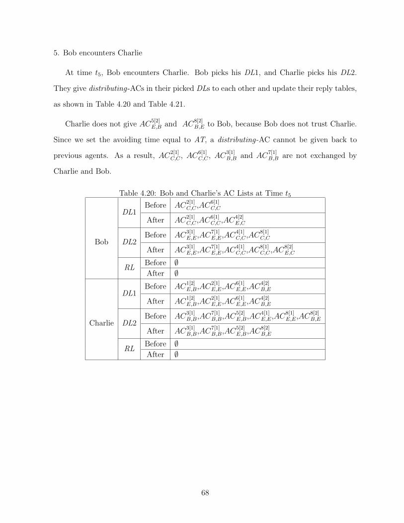
5. Bob encounters Charlie
At time t5, Bob encounters Charlie. Bob picks his DL1, and Charlie picks his DL2.
They give distributing-ACs in their picked DLs to each other and update their reply tables,
as shown in Table 4.20 and Table 4.21.
Charlie does not give AC5[2]E,B and AC
8[2]B,E to Bob, because Bob does not trust Charlie.
Since we set the avoiding time equal to AT, a distributing-AC cannot be given back to
previous agents. As a result, AC2[1]C,C , AC
6[1]C,C , AC
3[1]B,B and AC
7[1]B,B are not exchanged by
Charlie and Bob.
Table 4.20: Bob and Charlie’s AC Lists at Time t5
Bob
DL1Before AC
2[1]C,C ,AC
6[1]C,C
After AC2[1]C,C ,AC
6[1]C,C ,AC
4[2]E,C
DL2Before AC
3[1]E,E,AC
7[1]E,E,AC
4[1]C,C ,AC
8[1]C,C
After AC3[1]E,E,AC
7[1]E,E,AC
4[1]C,C ,AC
8[1]C,C ,AC
8[2]E,C
RLBefore ∅After ∅
Charlie
DL1Before AC
1[2]E,B,AC
2[1]E,E,AC
6[1]E,E,AC
4[2]B,E
After AC1[2]E,B,AC
2[1]E,E,AC
6[1]E,E,AC
4[2]B,E
DL2Before AC
3[1]B,B,AC
7[1]B,B,AC
5[2]E,B,AC
4[1]E,E,AC
8[1]E,E,AC
8[2]B,E
After AC3[1]B,B,AC
7[1]B,B,AC
5[2]E,B,AC
8[2]B,E
RLBefore ∅After ∅
68

Table 4.21: Bob and Charlie’s Relay Table At Time t5Bob Charlie
Aidold Aaptold IDnxt Aaptnew EQL Aidold Aaptold IDnxt Aaptnew EQL
B capt2B E aaptB(2)B 1 C capt2C B aapt
C(2)C 1
B capt4B E aaptB(4)B 1 C capt4C B aapt
C(4)C 1
B capt6B E aaptB(6)B 1 C capt6C B aapt
C(6)C 1
B capt8B E aaptB(8)B 1 C capt8C B aapt
C(8)C 1
B capt1B C aaptB(1)B 1 C capt1C E aapt
C(1)C 1
B capt3B C aaptB(3)B 1 C capt3C E aapt
C(3)C 1
B capt5B C aaptB(5)B 1 C capt5C E aapt
C(5)C 1
B capt7B C aaptB(7)B 1 C capt7C E aapt
C(7)C 1
E aaptE(1)E C aapt
E(1)B 2 B aapt
B(1)B E aapt
B(1)C 2
E aaptE(5)E C aapt
E(5)B 2 B aapt
B(5)B E aapt
B(5)C 2
E aaptE(4)E B aapt
E(4)C 2
E aaptE(8)E B aapt
E(8)C 2
6. Alice encounters Charlie
At time t6, Alice encounters Charlie. Alice picks her DL1, and Charlie picks his DL2.
They give distributing-ACs in their picked DLs to each other and update their reply tables,
as shown in Table 4.22 and Table 4.23.
69

Table 4.22: Alice and Charlie’s AC Lists at Time t6
Alice
DL1Before AC
1[0]A ,AC
3[0]A ,AC
5[0]A ,AC
7[0]A ,AC
2[2]B,E,AC
1[2]C,E
After AC2[2]B,E,AC
1[2]C,E,AC
3[2]B,C
DL2Before AC
6[2]B,E,AC
5[2]C,E
After AC6[2]B,E,AC
5[2]C,E,AC
7[2]B,C
RLBefore ∅After ∅
Charlie
DL1Before AC
1[2]E,B,AC
2[1]E,E,AC
6[1]E,E,AC
4[2]B,E
After AC1[2]E,B,AC
2[1]E,E,AC
6[1]E,E,AC
4[2]B,E,AC
1[1]A,A,AC
5[1]A,A
DL2Before AC
3[1]B,B,AC
7[1]B,B,AC
5[2]E,B,AC
8[2]B,E
After AC5[2]E,B,AC
8[2]B,E,AC
3[1]A,A,AC
7[1]A,A
RLBefore ∅After ∅
Table 4.23: Alice and Charlie’s Relay Table At Time t6Alice Charlie
Aidold Aaptold IDnxt Aaptnew EQL Aidold Aaptold IDnxt Aaptnew EQL
A capt2A E aaptA(2)A 1 C capt2C B aapt
C(2)C 1
A capt4A E aaptA(4)A 1 C capt4C B aapt
C(4)C 1
A capt6A E aaptA(6)A 1 C capt6C B aapt
C(6)C 1
A capt8A E aaptA(8)A 1 C capt8C B aapt
C(8)C 1
A capt1A C aaptA(1)A 1 C capt1C E aapt
C(1)C 1
A capt3A C aaptA(3)A 1 C capt3C E aapt
C(3)C 1
A capt5A C aaptA(5)A 1 C capt5C E aapt
C(5)C 1
A capt7A C aaptA(7)A 1 C capt7C E aapt
C(7)C 1
B aaptB(1)B E aapt
B(1)C 2
B aaptB(5)B E aapt
B(5)C 2
E aaptE(4)E B aapt
E(4)C 2
E aaptE(8)E B aapt
E(8)C 2
B aaptB(3)B A aapt
B(3)C 2
B aaptB(7)B A aapt
B(7)C 2
70
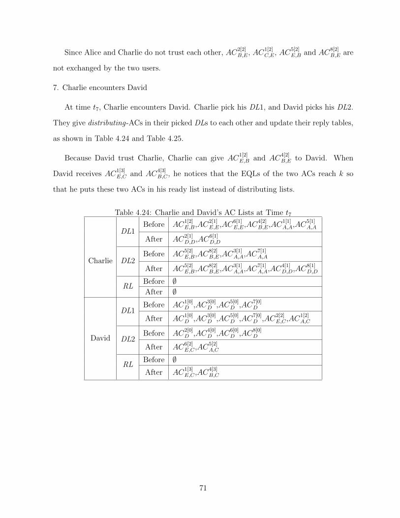
Since Alice and Charlie do not trust each other, AC2[2]B,E, AC
1[2]C,E, AC
5[2]E,B and AC
8[2]B,E are
not exchanged by the two users.
7. Charlie encounters David
At time t7, Charlie encounters David. Charlie pick his DL1, and David picks his DL2.
They give distributing-ACs in their picked DLs to each other and update their reply tables,
as shown in Table 4.24 and Table 4.25.
Because David trust Charlie, Charlie can give AC1[2]E,B and AC
4[2]B,E to David. When
David receives AC1[3]E,C and AC
4[3]B,C , he notices that the EQLs of the two ACs reach k so
that he puts these two ACs in his ready list instead of distributing lists.
Table 4.24: Charlie and David’s AC Lists at Time t7
Charlie
DL1Before AC
1[2]E,B,AC
2[1]E,E,AC
6[1]E,E,AC
4[2]B,E,AC
1[1]A,A,AC
5[1]A,A
After AC2[1]D,D,AC
6[1]D,D
DL2Before AC
5[2]E,B,AC
8[2]B,E,AC
3[1]A,A,AC
7[1]A,A
After AC5[2]E,B,AC
8[2]B,E,AC
3[1]A,A,AC
7[1]A,A,AC
4[1]D,D,AC
8[1]D,D
RLBefore ∅After ∅
David
DL1Before AC
1[0]D ,AC
3[0]D ,AC
5[0]D ,AC
7[0]D
After AC1[0]D ,AC
3[0]D ,AC
5[0]D ,AC
7[0]D ,AC
2[2]E,C ,AC
1[2]A,C
DL2Before AC
2[0]D ,AC
4[0]D ,AC
6[0]D ,AC
8[0]D
After AC6[2]E,C ,AC
5[2]A,C
RLBefore ∅After AC
1[3]E,C ,AC
4[3]B,C
71

Table 4.25: Charlie and David’s Relay Table At Time t7Charlie David
Aidold Aaptold IDnxt Aaptnew EQL Aidold Aaptold IDnxt Aaptnew EQL
C capt2C B aaptC(2)C 1 D capt2D C aapt
D(2)D 1
C capt4C B aaptC(4)C 1 D capt4D C aapt
D(4)D 1
C capt6C B aaptC(6)C 1 D capt6D C aapt
D(6)D 1
C capt8C B aaptC(8)C 1 D capt8D C aapt
D(8)D 1
C capt1C E aaptC(1)C 1
C capt3C E aaptC(3)C 1
C capt5C E aaptC(5)C 1
C capt7C E aaptC(7)C 1
B aaptB(1)B E aapt
B(1)C 2
B aaptB(5)B E aapt
B(5)C 2
E aaptE(4)E B aapt
E(4)C 2
E aaptE(8)E B aapt
E(8)C 2
B aaptB(3)B A aapt
B(3)C 2
B aaptB(7)B A aapt
B(7)C 2
B aaptE(1)B D aapt
E(1)C 3
E aaptE(2)E D aapt
E(2)C 2
E aaptE(6)E D aapt
E(6)C 2
E aaptB(4)E D aapt
B(4)C 3
A aaptA(1)A D aapt
A(1)C 2
A aaptA(5)A D aapt
A(5)C 2
8. David encounters Elizabeth
At time t8, David encounters Elizabeth. David picks his DL1, and Elizabeth picks her
DL2. They give distributing-ACs in their picked DLs to each other and update their reply
tables, as shown in Table 4.26 and Table 4.27.
After David gives Elizabeth the distributing-ACs, Elizabeth gets a ready-AC AC1[3]A,D.
72

Then Elizabeth has 1 ready-AC, while David has 2 ready-ACs, so that David has only
one more ready-ACs than Elizabeth. That is the reason why David does not give his own
ready-ACs to Elizabeth, even though Elizabeth trusts David.
We assume that Elizabeth does not get AC1[3]A,D, so that she has no ready-AC. Then
David should give her a ready-AC from his own two randomly.
Table 4.26: David and Elizabeth’s AC Lists at Time t8
David
DL1Before AC
1[0]D ,AC
3[0]D ,AC
5[0]D ,AC
7[0]D ,AC
2[2]E,C ,AC
1[2]A,C
After AC2[2]E,C ,AC
3[2]C,E,AC
4[2]A,E
DL2Before AC
6[2]E,C ,AC
5[2]A,C
After AC6[2]E,C ,AC
5[2]A,C ,AC
7[2]C,E,AC
8[2]A,E
RLBefore AC
1[3]E,C ,AC
4[3]B,C
After AC1[3]E,C ,AC
4[3]B,C
Elizabeth
DL1Before AC
1[2]B,C ,AC
2[1]A,A,AC
6[1]A,A
After AC1[2]B,C ,AC
2[1]A,A,AC
6[1]A,A,AC
1[1]D,D,AC
5[1]D,D
DL2Before AC
3[1]C,C ,AC
7[1]C,C ,AC
5[2]B,C ,AC
4[1]A,A,AC
8[1]A,A
After AC5[2]B,C ,AC
3[1]D,D,AC
7[1]D,D
RLBefore ∅After AC
1[3]A,D
73

Table 4.27: David and Elizabeth’s Relay Table At Time t8David Elizabeth
Aidold Aaptold IDnxt Aaptnew EQL Aidold Aaptold IDnxt Aaptnew EQL
D capt2D C aaptD(2)D 1 E capt1E B aapt
E(1)E 1
D capt4D C aaptD(4)D 1 E capt3E B aapt
E(3)E 1
D capt6D C aaptD(6)D 1 E capt5E B aapt
E(5)E 1
D capt8D C aaptD(8)D 1 E capt7E B aapt
E(7)E 1
D capt1D E aaptD(1)D 1 E capt2E C aapt
E(2)E 1
D capt3D E aaptD(3)D 1 E capt4E C aapt
E(4)E 1
D capt5D E aaptD(5)D 1 E capt6E C aapt
E(6)E 1
D capt7D E aaptD(7)D 1 E capt8E C aapt
E(8)E 1
C aaptA(1)C E aapt
A(1)D 3 B aapt
B(4)B C aapt
B(4)E 2
B aaptB(8)B C aapt
B(8)E 2
B aaptB(2)B A aapt
B(2)E 2
B aaptB(6)B A aapt
B(6)E 2
C aaptC(1)C A aapt
C(1)E 2
C aaptC(5)C A aapt
C(5)E 2
C aaptC(3)C D aapt
C(3)E 2
C aaptC(7)C D aapt
C(7)E 2
A aaptA(4)A D aapt
A(4)E 2
A aaptA(8)A D aapt
A(8)E 2
4.8.2 Queries and Replies
We still use the previous example and assume that the delivery of queries and replies cost
little time so that no AC expires in the period.
We assume that David wants to send a query to the LBS. He chooses a AC (e.g.
AC1[3]E,C) from his two ACs (i.e., AC
1[3]E,C and AC
4[3]B,C) randomly. If we review the previous
tables, we learn that AC1[3]E,C is generated by Elizabeth and has 3 agents (i.e., Elizabeth,
74

Bob and Charlie). When David uses the AC to send his query, the sender identity of
the query is Elizabeth. The Capt (i.e., capt1E) is also included in the query. Then David
uses the identity of the last agent (i.e., Charlie) and the Aapt (i.e., aaptE(1)C ) to generate
a pseudonym psdE(1)c = pseudo
(Charlie, aapt
E(1)c
), which is used as a temporary identity
of David before he receives the reply. Besides, AC1[3]E,C cannot be given to any user until it
expires. The process is shown in Figure 4.10.
Figure 4.10: David’s Query
The LBS sends a reply message to Elizabeth based on the sender identity of the query.
The Capt (i.e., capt1E) is also included in the reply. If an attacker learns these messages,
he believes that it is Elizabeth who sends the query.
When Elizabeth receives the reply message, she searches her reply table for the AC
used in the reply message, as shown in Table 4.27. Since the message is sent by the LBS,
the Aidold should equal to her own identity, and the Aaptold should equal to the Capt.
Then she must find an entry like Table 4.28, which enables Elizabeth to modify the reply
message and forward it to Bob, as shown in Figure 4.11.
Table 4.28: Elizabeth’s Reply Table EntryAidold Aaptold IDnxt Aaptnew EQL
E capt1E B aaptE(1)E 1
75

Figure 4.11: Elizabeth Forwards A Reply
If Bob receives the reply message successfully, he checks his reply table as shown in
Table 4.21. He finds an entry whose Aidold is equal to Elizabeth and Aaptold is equal to
aaptE(1)E , as shown in Table 4.29. In the same way as Elizabeth, Bob forwards the reply
message to Charlie, as shown in Figure 4.12.
Table 4.29: Bob’s Reply Table EntryAidold Aaptold IDnxt Aaptnew EQL
E aaptE(1)E C aapt
E(1)B 2
Figure 4.12: Bob Forwards A Reply
When the Charlie receives the reply message from Bob, Charlie learns that he is the
last agent based on his reply table as shown in Table 4.25 and Table 4.30, because the
EQL is equal to 3. He ignores the record of IDnxt D and views it as a V OID because he
is the last agent.
76

Table 4.30: Charlie’s Reply Table EntryAidold Aaptold IDnxt Aaptnew EQL
B aaptE(1)B D(V OID) aapt
E(1)C 3
To forward the reply message to the unknown original requester (i.e., David), Charlie
generates a pseudonym psdE(1)c = pseudo
(Charlie, aapt
E(1)c
)using his own identity and
Aaptnew. We should notice that the pseudonym is exactly the temporary identity of David.
David then modifies the reply message and forwards it, as shown in Figure 4.13.
Figure 4.13: Charlie Forwards A Reply
When a user who carries ReplyE(1)C encounters David, the user forwards the reply to
him, so that David gets his reply.
4.9 Experiment
We used the map of Helsinki in our simulator to evaluate performance of the proposed
ACP. We compare ACP with Binary Spray and Wait (BSW) protocol [25], distributed
social-based location privacy protocol (SLPD) [30] and our Multi-Hop Location-Privacy
Protection (MHLPP). We simulated the continuous movement of users along streets on
the map with one LBSP, fixed at a random location on the map.
77

For each user, we associate a random social value between 0 - 100%, each corresponding
to other users. Since each social value is assigned with equal probability, we can compute
the expected number of friends of an user. If an user whose social value is larger than 85%
is called a friend and there are n users in the network, then there are n× (1− 85%) friends
for this user in consideration.
The Shortest Path Map-Based Movement (SPMBM) [11] is used in our experiment for
the user mobility model. For each experiment, we give the simulator a random seed so
that it can generate a pseudo-random number based on the seed. Therefore, all the factors
including users’ speed and locations are the same if two experiments have the same random
seed. All four protocols are tested using the same set of random seeds.
Before each experiment, the simulator runs for 800 seconds, and then we pick 100 users
out of 126 users randomly to send a query to the LBSP. The simulation then lasts for 20
minutes before we measure different parameters for performance analysis.
4.9.1 Average Query Success Ratio
The query success ratio is the percentage of delivered queries among some attempts. Since
users sending 100 queries in each experiment, if s queries are delivered to the LBSP at
time t, the query success ratio of time t is s%.
As shown in Figure 4.14, we compare the average query success ratio of the four pro-
tocols for 5 different communication ranges (10, 30, 50, 70 and 90 meters) at 10 minutes
mark. We observe that our ACP and BSW achieve high query success ratio, while the
query success ratio in case of MHLPP and SLPD are lower than the other two. BSW has
the highest query success ratio because it is a no-privacy protocol. The ACP has slightly
lower query success ratio than BSW, because the query delivery process of the ACP is al-
most the same as that of BSW. Since users of ACP must wait for available ACs, it requires
more time to initiate their queries. However, ACP and BSW exhibit similar performance
78

compared to the other two protocols. MHLPP and SLPD need to find friends to obfuscate
their queries, which complicates their query delivery process.
Figure 4.14: Average Query Success Ratio (at 10 minutes mark)
The results at 20 minutes mark is shown in Figure 4.15. Both MHLPP and SLPD give
much higher query success ratio after 20 minutes than after 10 minutes. That is because
they require more time in their obfuscation phases when they need to find friends. In fact,
some of the queries of MHLPP and SLPD still do not finish their obfuscation phase at 20
minutes mark.
79

Figure 4.15: Average Query Success Ratio (at 20 minutes mark)
The communication range can influence the query success ratio. In most of the cases,
the success ratio rises when we increase the communication range, and its influence is
especially evident under 50 meters. A large communication range makes it easy for users
to encounter others, which is good for them to forward queries. However, an user who is
so far away from the destination does not want the intermediates of his query encounters
many users nearby. Because all users who carry copies of that query are near the sender
instead of the destination, which decreases their query success ratio. Therefore, when the
communication range reaches 70 meters, the success ratios almost stay flat.
In Figure 4.16, we observe that both ACP and BSW have better convergence speed
than MHLPP and SLPD. In other words, the former two protocols approach the 100%
query success ratio mark faster than the latter two. At the very beginning, the ACP even
has a little higher query success ratio than BSW. Because the ACP users need ready AC,
and most of the users get their first ready-ACs at places where there are many users, users
rarely generate query near the edges of the map at the beginning, which facilitates their
queries delivery process. For example, if an user generates his query at the edge of the
80

map, the copies of this query might be sent to users who are also at the edge, and it takes
more time for them to deliver the query. If the user does not generate his query until he
arrives at a place near the center, the copies of this query will be carried by the users in
the center with higher probability.
Figure 4.16: Average Query Success Ratio for 50-Meters Communication Range
4.9.2 Average Reply Success Ratio
When the LBSP receives a query, it sends a reply to the requester. If the reply reaches
the original requester before the test ends, we view it as a success; otherwise, the reply is
considered to be failed. There are three reasons for not receiving reply: 1) the query is not
delivered to the LBSP successfully; 2) the query took too much time for which the reply
could not be delivered in time; or 3) the route of the reply is too long. Since there are 100
queries in each experiment, we expect the number of replies should be 100.
In Figure 4.17, the BSW has a significantly higher reply success ratio than all other
protocols, because it is a no-privacy protocol. ACP has a higher ratio than MHLPP and
81
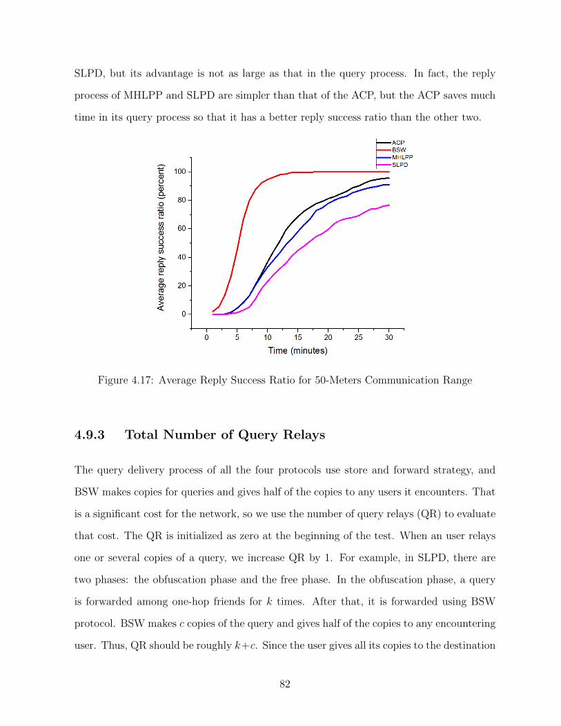
SLPD, but its advantage is not as large as that in the query process. In fact, the reply
process of MHLPP and SLPD are simpler than that of the ACP, but the ACP saves much
time in its query process so that it has a better reply success ratio than the other two.
Figure 4.17: Average Reply Success Ratio for 50-Meters Communication Range
4.9.3 Total Number of Query Relays
The query delivery process of all the four protocols use store and forward strategy, and
BSW makes copies for queries and gives half of the copies to any users it encounters. That
is a significant cost for the network, so we use the number of query relays (QR) to evaluate
that cost. The QR is initialized as zero at the beginning of the test. When an user relays
one or several copies of a query, we increase QR by 1. For example, in SLPD, there are
two phases: the obfuscation phase and the free phase. In the obfuscation phase, a query
is forwarded among one-hop friends for k times. After that, it is forwarded using BSW
protocol. BSW makes c copies of the query and gives half of the copies to any encountering
user. Thus, QR should be roughly k+c. Since the user gives all its copies to the destination
82

at once if he encounters the destination, the QR may be smaller. The smaller that number
is, the smaller the cost of the network is. Since there are 100 queries, we divide QR by 100
to get an average value.
In Figure 4.18, we compare QR in all four protocols. We observe that both BSW
and ACP have slightly lower QR than the other two. In case of ACP and BSW, they
deliver queries so fast that users who carry more than one copy give all their copies to the
destination before they send these copies to different users separately. As a result, many
copies have no chance to be forwarded, which decreases the cost.
While both MHLPP and SLPD have obfuscation phases, the queries start to be deliv-
ered freely (as in BSW) at a random place which might be so far away from the destination,
so that almost all copies can be forwarded.
Figure 4.18: Average Number of Forwarding Queries At 20 Minutes Mark
The communication range affects the total number of forwarding queries, especially in
the case of MHLPP and SLPD. These two protocols can finish their obfuscation phase more
quickly in a larger communication range scenario, so that more queries can be forwarded
freely (as in BSW), which makes their QR larger.
83

4.9.4 Memory Cost
We count the number of queries carried by each user to evaluate the memory cost of the
four protocols. Several copies of the same query are counted as one.
In Figure 4.19, we compare the number of queries per user in all four protocols at 20
minutes mark for different communication ranges. We observe that BSW has the highest
value in most of the cases whereas ACP always stays at a similar level as BSW. The average
query buffer needed per user in the other two protocols (MHLPP and SLPD) increases
with the increase in the communication range. The MHLPP even exceeds BSW when the
communication range is 90 meters. The reason is that quite a number of users in BSW
and ACP forward their copies to the destination so that there is no copy left with them
at 20 minutes mark, while the rest of them cannot forward their copies to the destination
even with large communication ranges. At the same time, the number of the other two
protocol’s free phase queries is significantly influenced by the communication range. The
more queries we have in the free phase, the more copies there are in the network.
Figure 4.19: Average Number of Query Buffer Needed at 20 Minutes Mark
84

The Figure 4.20 shows the average number of queries which are carried by users in
communication ranges 10, 50 and 90 meters. The curves for ACP and BSW rise sharply
at the beginning and then become flat, while those for MHLPP and SLPD rise smoothly
and continuously.
4.9.5 Distributing Appointment Cards
Exchanging ACs is a feature of proposed ACP, which can be considered as an extra cost.
We count the number of exchanging ACs per minute to evaluate this extra cost of ACP.
In Figure 4.21, we show the total number of exchanging ACs in the whole network. For
example, if an user Alice encounters another user Bob, the total number of exchanging ACs
processes increases by one when Alice exchanges any ACs to Bob. We count the number of
those exchanging processes occur per minute. As shown in the figure 4.21, the exchanging
processes do not occur frequently, but about 2 times per minutes. Since the size of an AC
is small, it does not consume too much network resource. At the same time, users can get
many ACs to help them send queries, as shown in Figure 4.22. The number of ready ACs
per user is raising smoothly and steadily.
85
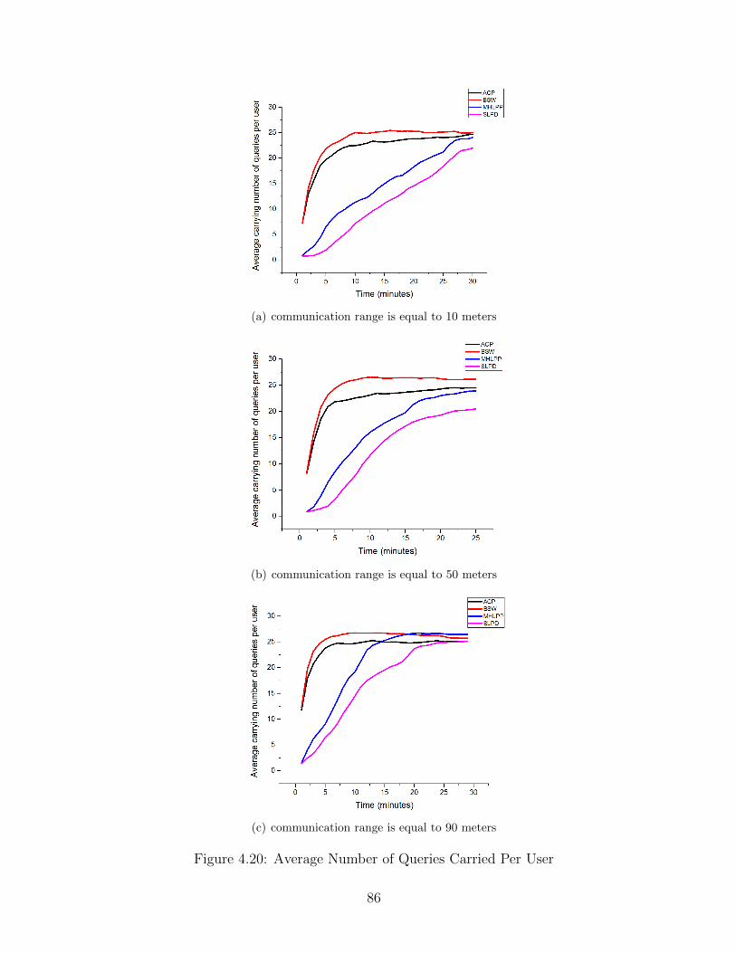
(a) communication range is equal to 10 meters
(b) communication range is equal to 50 meters
(c) communication range is equal to 90 meters
Figure 4.20: Average Number of Queries Carried Per User
86

Figure 4.21: Average Number of Exchanging ACs Per Minute Under Different Communi-cation Ranges
Figure 4.22: Average Number of Ready ACs Per User
87

Chapter 5
OMSN Routing Simulator (ORS)
The Opportunistic Networking Environment (ONE) [11] is a simulator designed for evalu-
ating DTN routing and application protocols. Researchers can import real-world map into
the simulator so that hosts walk along streets and roads in the simulator. The movement
model of hosts can be defined by researchers, which enables researchers to evaluate the
performance of their protocols in different scenarios. The User Interface of the ONE is
also friendly, where researchers can observe the movement of all hosts. When a round of
experiment ends, ONE outputs the results to a defined file. The simulator can also execute
in console mode, which allows a higher experiment speed.
The ONE is an excellent simulator for DTN research, while it has its own weakness.
The way that ONE estimates the distance between two hosts is not thorough, which may
lead to inaccurate results. When a host broadcasts a message, only the hosts which are
in its communication radius should receive the message. If the simulator cannot give the
accurate set of hosts which can receive the message, the experiment result is not reliable.
Although we can avoid this problem by setting parameters carefully, this problem cannot
be completely ignored. Besides, some movement models need to calculate shortest path
several times, which may require several seconds. Even though that is not a long time, it
can slow down the experiment speed significantly as the total time of a round of experiment
88

is about 10-20 seconds.
In this chapter, we introduce two major algorithms used in our new ORS simulator.
The vertex reduce algorithm is used for simplifying the input of the all-pair shortest path
algorithm, so that the simulator can initialize quickly. The finding nodes algorithm is used
to find users which are in the communication radius of a given user.
5.1 Overview
At its core, ORS is a discrete event simulation engine. To simulate an OMSN, hosts can
move in the simulator, and information of social network is also included in the simulator.
The simulator reads real-world maps, which enables hosts to walk along streets on the
maps. The default movement model of hosts is Working day movement model [5] where
hosts walk through the shortest path between several random points. Researchers can
replace the movement model with other models by implementing models in the source
codes.
The main function of ORS can be considered as the movement of hosts and message
routing. The movement routes of hosts is generated based on the movement model and are
defined by a series of segment lines before the simulation starts. In other words, the routes
are fixed before hosts start to walk so that the locations of hosts is a function of time.
Since ORS can get the locations of hosts directly when given a specific time value, it only
calculate locations of hosts when some hosts send messages or UI needs the locations of
hosts. Each host has a communication range which is a circle. ORS calculates the locations
of hosts when one or more hosts send messages, and the hosts inside the communication
range must receive the sent messages. The messages are always broadcast, and ORS copies
them to all hosts inside the communication range of the host who sends the message.
Therefore, the host itself decides whether a received message should be received or not,
which enables the hosts to control as many details as possible. The message structures
89

are defined by the implementation of DTN routing protocols and do not have mandatory
entries except a unique ID assigned by the simulator which is used for identifying messages.
The UI of ORS is shown in Figure 5.1. The parameters of the simulator which include
the file path of the map file, the number of hosts, the communication range and so on are
defined in a “txt” file. When we use ORS open the “txt” file (e.g., “aenv1.txt”), ORS reads
all parameters in the file and initialize the simulator. First, the simulator draws the map
and uses yellow lines to denotes the streets; second, ORS generates hosts, their relationship
strength, and their movement routes; third, ORS initializes instances of a specific routing
protocol for each host. ORS starts the experiment automatically when the initializations
finish. Users can define the values of the textboxes on the UI in source codes so that they
can debug their protocols.
Figure 5.1: Simulator UI
The hosts in the simulator can be viewed as mobile devices (e.g., smartphones) which
are a leak of software. These devices are carried by people who are moving in the sim-
90

ulator. ORS offers the devices interfaces so that users can implement routing protocols
which is the software of the mobile devices. The interfaces which devices can get from
ORS includes setting timers, current time, the identities of their owners, sending messages
to surroundings and so on. Comparing to ONE, the interfaces of ORS are more flexible
so that developers can almost define everything when they implement their routing pro-
tocols, like the size of buffers or the frequency of sending hello messages. ORS leaves the
implementation of persistent storage, energy consumption and message routing to routing
protocols instead of giving interfaces of these features, which enables researchers to make
their experiments more accurate. For example, the sizes of the messages are different. the
hello messages are small while general messages are large. Also, different operations cost
different energy. Therefore, it is good for developers to define these features by them self.
ORS can track all messages if developers implement the method by which ORS can iden-
tify messages. In this way, researchers can learn the location of each message, the number
of the message which is delivered to the destination, and the state of each message (e.g.,
shipping or delivered).
The relationship strengths of each pair of hosts are defined when ORS initials hosts.
The relationship strengths are fixed during the experiment. All relationship strengths are
recorded in a table so that routing protocols can get the relationship between any pair
of hosts when the protocols learn their identities. In general case, the routing protocols
can learn the identity of their owners and the identity of the senders of messages, so that
routing protocols can get the relationship strengths between the senders and their owners.
5.2 Vertex Reduction Algorithm
Movement of network nodes is a significant factor in the performance of DTNs. To evaluate
the performance of different DTN protocols, researchers have presented different kinds of
movement models, like in [5]. Since shortest path algorithm is an essential and time-cost
91

part of creating many movement models, it is an important aspect to optimize the time-cost
for simulators, calculating the all-pairs shortest paths in the entire map.
The best known non-negative edge weight undirected map all-pairs shortest path algo-
rithm [21] has a complexity O (n2logn ), which is still expensive when n is huge. For most
real-world city maps, there are thousands of points in a single square kilometer. Since a
ten-square kilometers map is reasonable for a DTN protocol evaluation, a simulator must
cut down the time spent in calculating all-pairs shortest paths to speed up the experiment.
Real-world map developers often use short straight lines to present curves, like in [1],
so that a several-meters curves may contain tens of points. It is obvious that we do not
need to calculate shortest path for every one of these points. In this chapter, we present
an Vertex Reduction Algorithm (VRA) to reduce the number of points before the use of
the shortest path algorithm. The basic idea is that VRA removes all points whose degrees
are less than 3 from the map, while keeping the result of all-pairs shortest path algorithm
correct.
The rest of this chapter is organized as follows. Section 5.2.1 presents some basic
definitions and lemmas. The process of VRA is described in Section 5.2.2 and Section
5.2.3.
5.2.1 Ignorable Vertex and Reserved Vertex
Vertices in the graph are considered ignorable and/or reserved (definition follows). In
each iteration of VRA, we remove the ignorable vertex from the graph, while the reserved
vertices compose a new graph.
Definition 1 : The vertex whose degree is larger than 2 is the reserved vertex (denoted
by R).
Definition 2 : The vertex whose degree is smaller than or equal to 2 is called the
ignorable vertex (denoted by G).
92

Definition 3 : If two reserved vertices (e.g. R1, R2) are connected by a sequence of
ignorable vertices (e.g. G1, G2, · · ·, Gn), then the sequence from R1 to R2 (i.e., R1, G1, G2,
· · · ,Gn, R2) is a line-segment (denoted by LS).
A reserved vertex can belong to different line-segments, while an ignorable vertex be-
longs to a unique line-segment. Both the reserved vertex and the ignorable vertex are
called vertices (V )
Definition 4 : The shortest route between two vertices inside a segment-line is called
the inner shortest path (SPI).
Let SPI (Vi, Vj) denote the inner shortest path between two vertices (i.e., Vi, Vj) inside
a segment-line.
Lemma 1 : If two vertices (i.e., Vi, Vj; i < j) are in the same line-segment, the shortest
path between them is
SP (Vi, Vj) = min {SPI (Vi, Vj) , SPI (R1, Vi) + SPI (Vj, R2) + SP (R1, R2)} (5.1)
Proof : Lemma 1 is shown in Figure 5.2. We assume that there is a path (e.g., Vi −
Vx− Vj) whose length is smaller than or equal to Equation 5.1 between Vi, Vj, where Vx is
a vertice in the segment-line including Vi, Vj.
Figure 5.2: Shortest Path On A Single Segment-Line
Case 1: Vx is between Vi and Vj. The length of the path Vi − Vx − Vj must be equal to
93

SPI (Vi, Vj) or there must be duplicated vertices on the path.
Case 2: Vx is between R1 and Vi or between Vj and R2. Vi − Vj should not be a part
of the path or Vi − Vj could be the shortest path. Then the path Vi − R1 − R2 − Vj must
be a part of Vi − Vx − Vj because R1 and R2 are entrances of the segment-line.
Since an all-pairs SPI has a complexity of O (n) and the n here is much smaller than
the number of points on the entire map, the time-cost for SPI is ignorable comparing to
the time-cost of the entire map all-pairs shortest path calculation.
Lemma 2 : We assume that there are two different line-segments
LSi = {Ri1, Gi1, Gi2, · · · , Gin, Ri2} and LSj = {Rj1, Gj1, Gj2, · · · , Gjm, Rj2}. We pick a
vertex Vi from LSi and a vertex Vj from LSj, then the shortest path between Vi and Vj is
SP (Vi, Vj) = min{SP (Vi, Ri1, Rj1, Vj) , SP (Vi, Ri2, Rj1, Vj) ,
SP (Vi, Ri1, Rj2, Vj) , SP (Vi, Ri2, Rj2, Vj)}(5.2)
where SP (Vi, Ria, Rjb, Vj) = SP (Vi, Ria) + SP (Ria, Rjb) + SP (Rjb, Vj). Here Vi and
Ria are in the same line-segment, so we can use Lemma 1 to calculate SP (Vi, Ria), so does
SP (Rjb, Vj). The SP (Ria, Rjb) is the only part we need to calculate using all-pair shortest
path algorithms. We should notice that Ria and Rjb could be the same vertex, but it does
not make any difference to the lemma.
Proof : Since Vi and Vj are not in the same segment-line, there must be one or more
reserved vertices on their shortest path. On Vi’s side, one of Ri1 and Ri2 must be on the
shortest path. One of Rj1 and Rj2 should be on that shortest path, either. We assume
that Riu and Rjv are on the shortest path between Vi and Vj, then a shortest path between
Riu and Rjv should be a part of that path.
94

5.2.2 Vertex Reduction
VRA iteratively removes ignorable vertices from the graph until only reserved vertices
remain. In each iteration, we remove all ignorable vertices from the graph but keep the
edges. If there are different routes between a pair of reserved vertices, we keep the shortest
one and remove others.
5.2.2.1 Remove Ignorable Vertices
Since the degree of ignorable vertices is no more than 2, an ignorable vertex has only 0,
1 or 2 neighbours. In the case of 0 or 1 neighbour, we simply delete the ignorable vertex;
if it has two neighbours, we connect its two neighbours before it is removed, as shown in
Figure 5.3. When we remove an ignorable vertex, the weight of the line which connects its
two neighbours is equal to the sum of its recent two lines’ weights (i.e., Wl + Wr). After
we remove all ignorable vertices in a line-segment, the two reserved vertices at the end
of the line-segment are connected with a line directly, whose weight is the sum of all the
intermediate ones’ (i.e., W1 +W2 +W3 +W4).
Figure 5.3: Remove Ignorable Vertices
5.2.2.2 Remove Redundant Connections
After we remove all ignorable vertices, all the reserved vertices are connected directly.
However, it is possible that there are several connections between a pair of reserved vertices.
Since the shortest route between a pair of neighbouring vertices makes other longer ones
95

redundant, we remove all routes except the shortest one, as shown in Figure 5.4. We assume
that W2 is the shortest line among three connections, when W1 and W3 are removed.
Figure 5.4: Tidy Reserved Connections
5.2.2.3 Iterations
The process is shown in Algorithm 5.1. The input of the algorithm is the original en-
tire map, which is called Graph0. In the i th iteration, VRA makes a copy of Graphi as
Graphi+1. If i > 0, the Graphi is the output of the previous (i.e., (i− 1)th) iteration. VRA
removes all ignorable vertices in the Graphi+1 as described in Section 5.2.2.1 and remove
all unnecessary routes between reserved vertices as described in Section 5.2.2.2. In other
words, Graphi gets smaller and smaller as i increases, because we always remove ignorable
vertices from them. If Graphi is equal to Graphi+1, which means that the i th iteration
makes no modification on the graph, the algorithm ends.
5.2.3 Assembling Vertices
We assume that the vertex reduction process stops at the i th iteration. Then, the Graphi
is the input of an all-pairs shortest path algorithm. Let SPi (Ru, Rv) denote the shortest
path from Ru to Rv in Graphi. We can infer the all-pairs shortest path of Graphi−1 based
on Graphi with Lemma 1 and Lemma 2. The algorithm ends when we get the result of
Graph0. The algorithm is shown in Algorithm 5.2.
We start from the Graphi−1 and assemble all intermediate graphs, until we get the result
of Graph0. For any intermediate Graphj, we already have the all-pairs shortest path
96
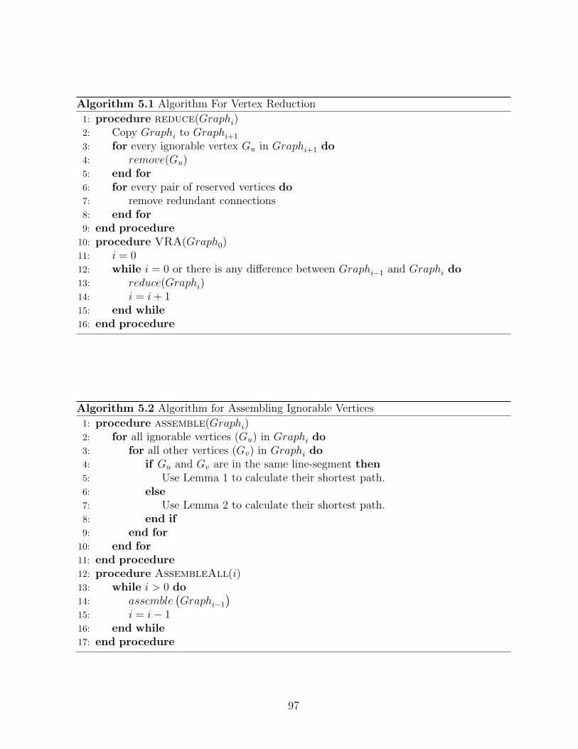
Algorithm 5.1 Algorithm For Vertex Reduction
1: procedure reduce(Graphi)2: Copy Graphi to Graphi+1
3: for every ignorable vertex Gu in Graphi+1 do4: remove(Gu)5: end for6: for every pair of reserved vertices do7: remove redundant connections8: end for9: end procedure10: procedure VRA(Graph0)11: i = 012: while i = 0 or there is any difference between Graphi−1 and Graphi do13: reduce(Graphi)14: i = i+ 115: end while16: end procedure
Algorithm 5.2 Algorithm for Assembling Ignorable Vertices
1: procedure assemble(Graphi)2: for all ignorable vertices (Gu) in Graphi do3: for all other vertices (Gv) in Graphi do4: if Gu and Gv are in the same line-segment then5: Use Lemma 1 to calculate their shortest path.6: else7: Use Lemma 2 to calculate their shortest path.8: end if9: end for10: end for11: end procedure12: procedure AssembleAll(i)13: while i > 0 do14: assemble
(Graphi−1
)15: i = i− 116: end while17: end procedure
97

result of its reserved vertices in the previous iteration (i.e., Graphj+1). Then, we calculate
the shortest path from any ignorable vertex to all others. When the two vertices are in
the same line-segment, we use Lemma 1 to calculate their shortest path. The Lemma 1
includes four parts: SPI (Vi, Vj), SPI (R1, Vi), SPI (Vj, R2) and SP (R1, R2). Since we
already have the result of SP (R1, R2) in the previous iteration, we just need to calculate
the remaining three SPI parts, which is easy and has fewer nodes. If the two vertices are
in different line-segments, we use Lemma 2 to calculate the shortest path. We already have
all the SP parts from the previous iteration, so we just need to deal with their respective
SPI parts.
5.3 Finding Nodes in a Range
We assume that there are n nodes in a planar map (size: h×w). Those nodes keep moving
on the map slower than a speed threshold (S). If the distance between two nodes a and b is
smaller than r, they are considered connected. We want to calculate all-pairs connections
for all nodes on the map periodically.
If we calculate these connections directly, the complexity is O(n2
2
). We assume that
r � min {h,w}, and nodes are distributed on the entire map symmetrically. Then, the
expected number of nodes which has a connection with a node (v) is nh×w × πr
2 � n. If
we traverse all other (n− 1) nodes of v, it will be a waste of time.
We propose an algorithm to optimize the calculation of all-pairs connections. We draw
grids whose size is l × l on the map. When we calculate connections of the node v, only
nodes in surrounding grids will be traversed.
98

5.3.1 Static Nodes
If nodes on the map are stationary, the r is the only factor of the selection of the grid size
(l× l). The length l of the side of a grid should be equal to r, as shown in Figure 5.5. For
any node v in the dark grid, all nodes whose distance between them is equal to or shorter
than r should be in the grey or dark grid. Therefore, if we want to get all connected nodes
to node v, we simply need to traverse all nodes in the grey and dark grids instead of all
nodes in the entire map. In this case, the expected number of nodes which we need to
traverse is 9n×r2h×w for checking connections for a node v. If we calculate connections for all
nodes, we simply need to get the distances of about 9n2×r22×h×w pairs of nodes, instead of n2
2
pairs.
Figure 5.5: Grid Size For Still Nodes
5.3.2 Mobile Nodes
The problem is a bit more complicated if nodes are moving. Assuming that we want to
calculate all-pairs connections at t1, first, we draw grids at time t0, so that we know which
grid is a node in at t0. Instead of t0, we want to get connections at t1. In this case, the
length l should be larger than r.
Suppose that we have two nodes u and v, and their distance is d1 at t1. Since the
99

maximum speed of nodes is S, their distance d0 at t0 satisfies
max {0, d1 − 2δ} ≤ d0 ≤ d1 + 2δ
where δ = S |t1 − t0|. When d1 ≤ r, these two nodes are connected at t1, then d0 must
satisfy 0 ≤ d0 ≤ r+2δ. As shown in Figure 5.6, If we draw grids on the map in an attempt
to place the two nodes in the same or adjacent grids at t0, the length of each grid l = r+2δ.
Figure 5.6: Length of Grid
5.3.3 Complexity
The complexity of drawing grids is O (n), while that of checking connections is O(
9n2×l22×h×w
),
so the checking part is much more expensive than the drawing part. Since l = r + 2δ =
r + 2S |t1 − t0|, the checking part achieves its best performance when t1 − t0 = 0, then its
complexity is O(
9n2×r22×h×w
). That is equal to the complexity when nodes are stationary.
100

Chapter 6
Conclusion and Future Work
In this chapter, we will summarize our findings and discuss the future directions of the
proposed work in the previous chapters yet to be explored.
6.1 Summary of Work Done
In this thesis, we proposed and analyzed two new location-privacy preserving protocols,
namely MSLPP and ACP, besides developing a new OMSN simulator, called ORS, as a
platform for evaluating the proposed protocols and comparing them with their counter-
parts.
Our first protocol, MSLPP, is a distributed location-privacy preserving protocol using
social-relationship and encryption. Simulation results show that it has a better perfor-
mance on delivery success ratio and provides an acceptable obfuscation compared to its
counterpart HSLPO which is an improvement of their earlier scheme SLPD. Compared to
HSLPO, our scheme MHLPP achieves an in increase in success ratio between 6% and 11%
for the same range of parameters considered by the authors of SLPD. The success ratios
of both HSLPO and MHLPP decline when the privacy threshold is increased, while the
success ratio of HSLPO is always lower than that of MHLPP and decreases more sharply
101

than that of MHLPP. Although HSLPO is slightly more secure than MHLPP based on
our experiments which means the original requester has a lower rate to be located, but
the entropy difference is quite small and negligible. Encryption and decryption to enhance
security are added cost for MHLPP which is acceptable. Our experiment (using the map of
Helsinki) presents that in a social network with 126 users, the average number of times of
a query is encrypted and decrypted is less than 3 when the privacy threshold is considered
as 85.
Our second proposed Appointment Card Protocol ACP also uses social relationship for
preserving location privacy. It facilitates the obfuscation process by continuously exchang-
ing appointment cards among users so that the original requester does not communicate
with any of its friends when initiating a query. Simulation results show that it has a better
performance with respect to the query-delivery success ratio and provides an acceptable
obfuscation compared to its counterparts. Although ACP requires slightly more time to
forward the reply, the total time required for query delivery and reply delivery is still less
than that for its counterparts SLPD and MHLPP.
To facilitate our experimentation, we have developed a simulator, called ORS, which is
more suitable for OMSN simulation than the existing simulator, ONE. The ORS is more
reliable and efficient than ONE for simulating opportunistic social networks.
6.2 Future Work
In MHLPP, we just considered the relationship strength between two connected people in
the social network; in other words, an agent only gives the message to his direct friend.
In most of the cases, the friends of your friends can also be trusted and be considered.
If these friends can participate in forwarding queries, agents can have more choice in the
obfuscation phase.
In ACP, the sizes of agents’ relay tables are significantly affected by the number of
102
appointment cards passing by them. If we can decrease the number of appointment cards
in the network, the burden of agents can also decline. For example, a single appointment
card can be shared among friends instead of being used by only one user.
103

References
[1] Openstreetmap, 2017. https://www.openstreetmap.org/.
[2] L. J. Chen, C. H. Yu, T. Sun, Y. C. Chen, and H. H. Chu. A hybrid routing approach
for opportunistic networks. In the 2006 SIGCOMM workshop on Challenged networks
(CHANTS), pages 213–220, September 2006.
[3] W. Diffie and M. E. Hellman. New directions in cryptography. IEEE Transactions on
Information Theory, 22(6):644–654, November 1976.
[4] M. Duckham. Moving forward: Location privacy and location awareness. In the
3rd ACM International Workshop on Security and Privacy in GIS and LBS. ACM,
November 2010.
[5] F. Ekman, A. Keranen, J. Karvo, and J. Ott. Working day movement model. In the
1st ACM SIGMOBILE workshop on Mobility models, pages 33–40. ACM, May 2008.
[6] K. Fall. A delay-tolerant network architecture for challenged internets. In the Confer-
ence on Applications, Technologies, Architectures, and Protocols for Computer Com-
munications, pages 27–34, 2003.
[7] C. Chow J. Zhang. Real: A reciprocal protocol for location privacy in wireless sensor
networks. IEEE Transactions on Dependable and Secure Computing, 12(4):458–471,
October 2014.
104

[8] P. Jacquet, P. Muhlethaler, and T. Clausen. Optimized link state routing protocol for
ad hoc networks. In IEEE International Multi Topic Conference 2001 - IEEE INMIC
2001. IEEE, December 2001.
[9] E. P. Jones and P. A. Ward. Routing strategies for delay-tolerant networks. ACM
CCR, 2006.
[10] E. P. C. Jones, L. Li, and J. K. Schmidtke. Practical routing in delay-tolerant networks.
IEEE Transactions on Mobile Computing, 6(8):943 – 959, June 2007.
[11] A. Keranen, J. Ott, and T. Karkkainen. The one simulator for dtn protocol evaluation.
In the 2nd International Conference on Simulation Tools and Techniques. ICST, March
2009.
[12] John Krumm. A survey of computational location privacy. Personal and Ubiquitous
Computing, 13(6):391–399, August 2009.
[13] U. Lee, S. Y. Oh, K. W. Lee, and M. Gerla. Relay cast: scalable multicast routing
in delay tolerant networks. In IEEE International Conference on Network Protocols,
pages 218–227, October 2008.
[14] Y. Liao, K. Tan, Z. Zhang, and L. Gao. Estimation based erasure coding routing in
delay tolerant networks. In the 2006 international conference on Wireless communi-
cations and mobile computing (IWCMC), pages 557–562, July 2006.
[15] A. Lindgren, A. Doria, and O. Schelen. Probabilistic routing in intermittently con-
nected networks. ACM SIGMOBILE Mobile Computing and Communications Review,
7(3):19–20, July 2003.
[16] C. Liu and J. Wu. Scalable routing in delay tolerant networks. In the 8th ACM
international symposium on Mobile ad hoc networking and computing, pages 51–60.
ACM, 2007.
105

[17] R. Lu, X. Lin, and X. Shen. Spring: A social-based privacy-preserving packet for-
warding protocol for vehicular delay tolerant networks. In 2010 Proceedings IEEE
INFOCOM. IEEE, March 2010.
[18] D. Grunwald M. Gruteser. Anonymous usage of location-based services through spa-
tial and temporal cloaking. In the 1st International Conference on Mobile Systems,
Applications and Services, pages 31–42, May 2003.
[19] M. Mano and Y. Ishikawa. Anonymizing user location and profile information for
privacy-aware mobile services. In the 2nd ACM SIGSPATIAL International Workshop
on Location Based Social Networks, pages 68–75. ACM, November 2010.
[20] C. Mascolo, S. Hailes, L. Lymberopoulos, G. P. Picco, P. Costa, G. Blair, P. Okanda,
T. Sivaharan, W. Fritsche, M. Karl, M. A. Ronai, K. Fodor, and A. Boulis. Reconfig-
urable ubiquitous networked embedded systems. Technical report, January 2005.
[21] A. Moffat and T. Takaoka. all pairs shortest path algorithm with expected running
time o(n2logn). In 26th Annual Symposium on Foundations of Computer Science.
IEEE, October 1985.
[22] A.K. Pietilainen. Opportunistic Mobile Social Networks at Work. PhD thesis, Univer-
site Pierre et Marie Curie, Paris, 2010.
[23] E. Reddy, S. Kumar, N. Rollings, and R. Chandra. Mobile application for dengue fever
monitoring and tracking via gps: Case study for fiji. Technical Report TR-04-2015,
Mar 2015.
[24] J. Schiller and A. Voisard. Location-Based Services. Morgan Kaufmann, 2004.
[25] T. Spyropoulos, K. Psounis, and C. S. Raghavendra. Spray and wait: An efficient
routing scheme for intermittently connected mobile networks. In the ACM SIGCOMM
Workshop on Delay-tolerant Networking, pages 252–259. ACM, August 2005.
106

[26] L. Liu T. Wang. Privacy-aware mobile services over road networks. the VLDB En-
dowment, 2(1):1042–1053, August 2009.
[27] A. Vahdat and D. Becker. Epidemic routing for partially-connected ad hoc networks.
Technical Report CS-2000-06, April 2000.
[28] R. Xiang, J. Neville, and M. Rogati. Modeling relationship strength in online social
networks. In the 19th International Conference on World Wide Web, pages 644–654.
ACM, April 2010.
[29] X. Xue, J. Li, Y. Cao, and J. Fang. Advanced prophet routing in delay tolerant net-
work. In IEEE International Conference on Communication Software and Networks.
IEEE, 2009.
[30] S. Zakhary and M. Radenkovic. Utilizing social links for location privacy in oppor-
tunistic delay-tolerant networks. In International Conference on Communications
(ICC). IEEE, June 2012.
[31] S. Zakhary, M. Radenkovic, and A. Benslimane. The quest for location-privacy in
opportunistic mobile social networks. In Wireless Communications and Mobile Com-
puting Conference (IWCMC). IEEE, July 2013.
[32] S. Zakhary, M. Radenkovic, and A. Benslimane. Efficient location privacy-aware for-
warding in opportunistic mobile networks. IEEE Transactions on Vehicular Technol-
ogy, 63(2):893–906, February 2014.
[33] M. M. Zanjireh and H. Larijani. A survey on centralised and distributed clustering
routing algorithms for wsns. In Vehicular Technology Conference (VTC Spring). IEEE,
May 2015.
107