Proton form factors: Interesting at all scales
84
Proton form factors: Interesting at all scales Jan C. Bernauer SPhN Seminar Saclay, October 2013 OL MPUS 1
Transcript of Proton form factors: Interesting at all scales

Proton form factors: Interesting at all scales
Jan C. Bernauer
SPhN Seminar Saclay, October 2013
OL MPUS
1

Overview
MotivationHigh Q2: Two-Photon-ExchangeMiddle Q2: Pushing the precision boundaryLow Q2: The size of the protonNew data
2
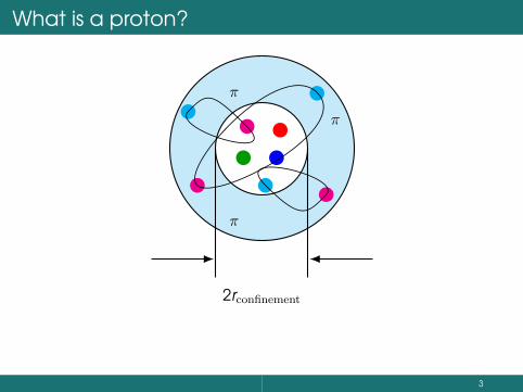
What is a proton?
2rconfinement
π
π
π
3

Cross section and form factors for elastic e-pscattering
The cross section:(dσdΩ
)(
dσdΩ
)Mott
=1
ε (1 + τ)
[εG2
E
(Q2)
+ τG2M
(Q2)]
with:τ =
Q2
4m2p, ε =
(1 + 2 (1 + τ) tan2 θe
2
)−1
Fourier-transform of GE , GM −→spatial distribution(Breit frame)
⟨r2E
⟩= −6~2 dGE
dQ2
∣∣∣∣Q2=0
⟨r2M
⟩= −6~2 d (GM/µp)
dQ2
∣∣∣∣Q2=0
4

Unpolarized: Rosenbluth
0.001
0.01
0.1
1
10
100
1965 1970 1975 1980 1985 1990 1995 2000 2005 2010
Q2/(G
eV/c)2
YearAndivahisBartelBergerBernauer
BorkowskiBostedChristyGoitein
JanssensLittPriceQattan
RockSillSimonStein
Walker
5

Polarized: Ratio
0.001
0.01
0.1
1
10
100
1965 1970 1975 1980 1985 1990 1995 2000 2005 2010
Q2/(GeV
/c)
2
Yearunpolarized
CrawfordDieterich
GayouJones
MacLachlanMezianeMilbrath
PospischilPuckett
PunjabiRon
Zhan
6

Large Q2
Q2Q2
Q2
7

Ratio: Difference!
0
0.2
0.4
0.6
0.8
1
1.2
1.4
1.6
0 1 2 3 4 5 6 7 8 9 10
µpG
E/G
M
Q2/(GeV/c)2
Rosenbluth Polarization
8
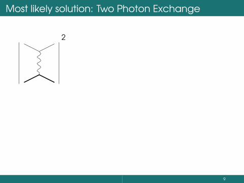
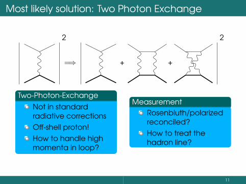
Most likely solution: Two Photon Exchange
2
=⇒ + +
2
Two-Photon-Exchange
Not in standardradiative correctionsOff-shell proton!How to handle highmomenta in loop?
MeasurementRosenbluth/polarizedreconciled?How to treat thehadron line?
9

Most likely solution: Two Photon Exchange
2
=⇒ + +
2
Two-Photon-Exchange
Not in standardradiative correctionsOff-shell proton!How to handle highmomenta in loop?
MeasurementRosenbluth/polarizedreconciled?How to treat thehadron line?
10
Most likely solution: Two Photon Exchange
2
=⇒ + +
2
Two-Photon-Exchange
Not in standardradiative correctionsOff-shell proton!How to handle highmomenta in loop?
MeasurementRosenbluth/polarizedreconciled?How to treat thehadron line?
11

Measure TPE
Interference termchanges sign withlepton sign!Measured in the 1960sNot much dataA lot of predictions!
e+/e
−-
ratio
ε
Yount+Pine 1962Browman 1965
Mar 1968Bouquet 1968
Yang phen.Guttmann phen.
AfanasevBlunden (g.s.)
Blunden (g.s. + ∆)Borisyuk (g.s.)
Gorchtein (inel.)
0.95
1
1.05
1.1
1.15
1.2
0 0.2 0.4 0.6 0.8 1
12
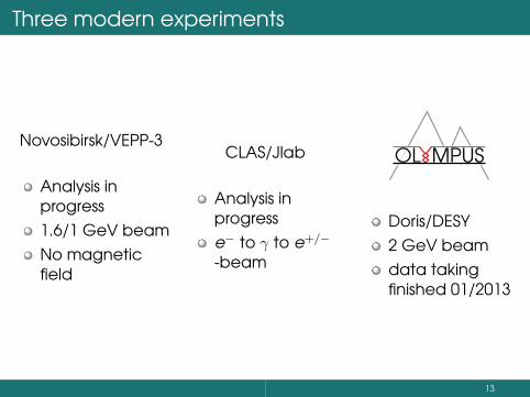
Three modern experiments
Novosibirsk/VEPP-3
Analysis inprogress1.6/1 GeV beamNo magneticfield
CLAS/Jlab
Analysis inprogresse− to γ to e+/−
-beam
OL MPUS
Doris/DESY2 GeV beamdata takingfinished 01/2013
13

The OLYMPUS collaboration
Arizona State University, USADESY, Hamburg, GermanyHampton University, USAINFN, Bari, ItalyINFN, Ferrara, ItalyINFN, Rome, ItalyMIT Laboratory for Nuclear Science, Cambridge, USASt. Petersburg Nuclear Physics Institute, St. Petersburg,RussiaUniversity of Bonn, Bonn, GermanyUniversity of Glasgow, United KingdomUniversity of Mainz, Mainz, GermanyUniversity of New Hampshire, USAYerevan Physics Institute, Armenia
14

At DESY: DORIS
15

Projected performance
e+/e
−-
ratio
ε
Yount+Pine 1962Browman 1965
Mar 1968Bouquet 1968
Olympus projected
Yang phen.Guttmann phen.
AfanasevBlunden (g.s.)
Blunden (g.s. + ∆)Borisyuk (g.s.)
Gorchtein (inel.)
0.95
1
1.05
1.1
1.15
1.2
0 0.2 0.4 0.6 0.8 1
2 GeV beam, Q2-range: 0.6 to 2.2 GeV2
16

Target / Vacuum
Beam direction
17
Open cell designCryogenicTarget density: 3 · 1015 cm−2
Multi-stage pump system

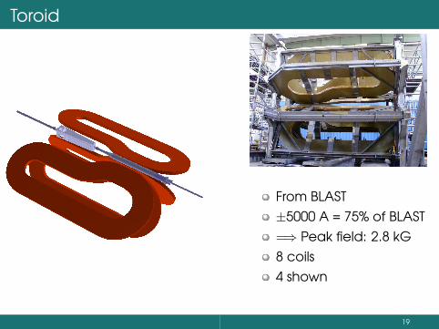
Toroid
18
From BLAST±5000 A = 75% of BLAST=⇒ Peak field: 2.8 kG8 coils
4 shown
Toroid
19
From BLAST±5000 A = 75% of BLAST=⇒ Peak field: 2.8 kG8 coils4 shown

Wire chamber
20
From BLASTHDC design, 3 signalwirescompletely rewired2 · 3 planes / chamber,3 chambers / side10 stereo angle

Time Of Flight
21
From BLASTRewrapped, testedTrigger
Top/bottom coinc.kinematicallyconstrained
+ 2nd level WC

Time Of Flight
22
From BLASTRewrapped, testedTrigger
Top/bottom coinc.kinematicallyconstrained+ 2nd level WC

Luminosity
23
Tight control crucial!Redundant systems:
12-detector(Hampton, PNPI)SymmetricMøller/Bhabha (Mainz)

12-detector
umin
24
3 GEM (Hampton) + 3MWPC (PNPI) eachhighly redundantSiPM triggerscintillators

Symmetric Møller/Bhabha
25
2×9 crystals (Mainz)1.3 symmetric anglehigh rate, no deadtime
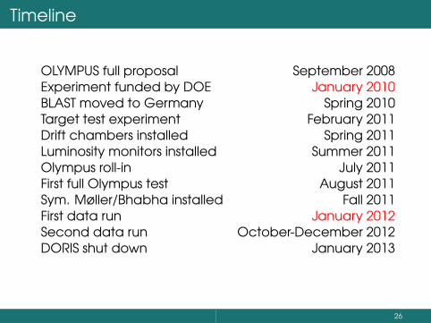
Timeline
OLYMPUS full proposal September 2008Experiment funded by DOE January 2010BLAST moved to Germany Spring 2010Target test experiment February 2011Drift chambers installed Spring 2011Luminosity monitors installed Summer 2011Olympus roll-in July 2011First full Olympus test August 2011Sym. Møller/Bhabha installed Fall 2011First data run January 2012Second data run October-December 2012DORIS shut down January 2013
26

Luminosity
Inte
grat
edLu
min
osity
[fb−1]
Date
Electron, positive toroid: 1.93 fb−1
Positron, positive toroid: 1.96 fb−1
Electron, negative toroid: 0.24 fb−1
Positron, negative toroid: 0.32 fb−1
Total: 4.45 fb−1
0
0.5
1
1.5
2
2.5
3
3.5
4
4.5
Jan ’12 Mar ’12 May ’12 Jul ’12 Sep ’12 Nov ’12 Jan ’13
Exceeded goal for integrated luminosity: > 4 fb−1
27

Analysis
CAVEAT: The analysis has just started. All plots arepreliminary.
28
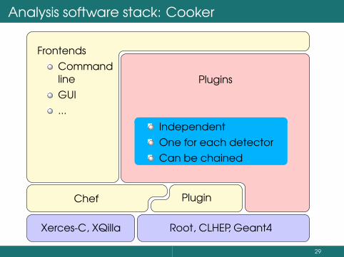
Analysis software stack: Cooker
Xerces-C, XQilla Root, CLHEP, Geant4
Chef Plugin
FrontendsCommandlineGUI...
Plugins
IndependentOne for each detectorCan be chained
29

Plugin System
Raw
data
SlowCtrl
Time Of Flight
Wire Chamber
LumiGEM
MWPC
Møller
LumiTrack
TrackFit
eP elastic
Pions
...
30
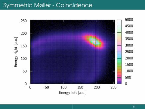
Symmetric Møller - Coincidence
Ener
gyrig
ht[a
.u.]
Energy left [a.u.]
0
50
100
150
200
250
0 50 100 150 200 2500
500
1000
1500
2000
2500
3000
3500
4000
4500
5000
Symmetric Møller/Bhabha
31

Symmetric Møller - Coincidence
Ener
gyrig
ht[a
.u.]
Energy left [a.u.]
0
50
100
150
200
250
0 50 100 150 200 2500
500
1000
1500
2000
2500
3000
3500
4000
4500
5000
Symmetric Møller/Bhabha
32

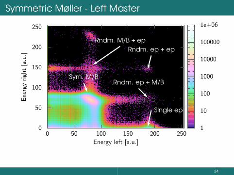
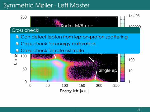
Symmetric Møller - Left MasterEn
ergy
right
[a.u
.]
Energy left [a.u.]
0
50
100
150
200
250
0 50 100 150 200 2501
10
100
1000
10000
100000
1e+06
Sym. M/B
Rndm. M/B + ep
Rndm. ep + M/B
Rndm. ep + ep
Single ep
Cross check!Can detect lepton from lepton-proton scatteringCross check for energy calibrationCross check for rate estimate
33
Symmetric Møller - Left MasterEn
ergy
right
[a.u
.]
Energy left [a.u.]
0
50
100
150
200
250
0 50 100 150 200 2501
10
100
1000
10000
100000
1e+06
Sym. M/B
Rndm. M/B + ep
Rndm. ep + M/B
Rndm. ep + ep
Single ep
Cross check!Can detect lepton from lepton-proton scatteringCross check for energy calibrationCross check for rate estimate
34
Symmetric Møller - Left MasterEn
ergy
right
[a.u
.]
Energy left [a.u.]
0
50
100
150
200
250
0 50 100 150 200 2501
10
100
1000
10000
100000
1e+06
Sym. M/B
Rndm. M/B + ep
Rndm. ep + M/B
Rndm. ep + ep
Single ep
Cross check!Can detect lepton from lepton-proton scatteringCross check for energy calibrationCross check for rate estimate
35
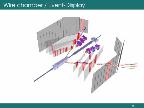
Wire chamber / Event-Display
36

Reconstructed proton momentum(p(θ)−pmeasured) p
roton
[MeV
]
Proton scattering angle
"ep.dat" u 1:2:3 index 146
0
500
1000
1500
2000
0 20 40 60 80 1000
100
200
300
400
500
600
700
800
PRELIMINARY!Will change!Small subset of data from first run.
37

Middle Q2
Q2Q2
Q2
38

Motivation: Structure
0.4
0.6
0.8
1
1.2
1.4
1.6
0 1 2 3 4 5 6
GE
P/G
dip
ole
Q / (GeV/c)
totalsmooth
Simon et al.Price et al.
Berger et al.Hanson et al.
polarisation data
0.4
0.6
0.8
1
1.2
1.4
1.6
0 1 2 3 4 5 6
GM
P/(
µpG
dip
ole
)
Q / (GeV/c)
totalsmooth
Hoehler et al.Janssens et al.
Berger et al.Bartel et al.
Walker et al.Litt et al.
Andivahis et al.Sill et al.
-0.1
-0.05
0
0.05
0.1
0.001 0.01 0.1 1 10
GE
P-G
EP
,sm
ooth
Q2 / (GeV/c)
2
total-smoothSimon et al.Price et al.
Berger et al.Hanson et al.
polarisation data
-0.1
-0.05
0
0.05
0.1
0.001 0.01 0.1 1 10
GM
P-G
MP
,sm
ooth
Q2 / (GeV/c)
2
total - smoothHoehler et al.
Janssens et al.Berger et al.Bartel et al.
Walker et al.Litt et al.
Andivahis et al.Sill et al.
(see J. Friedrich and Th. Walcher, Eur. Phys. J. A 17 (2003) 607)39

High-precision p(e,e’)p measurement at MAMI
Three spectrometer facility of the A1 collaboration:
40
Design goal: High precision
Statistical precision: 20 min beam time for <0.1%
Control of luminosity and systematic errors:
Redundancy!
Redundant beam current measurementFoerster probe⇐⇒ pA-meter
Redundant luminosity:current × density × target length⇐⇒ spectrometer asmonitor
Overlapping acceptanceWhere possible: Measure at the same scatteringangle with two spectrometers
41

Design goal: High precision through redundancy
Statistical precision: 20 min beam time for <0.1%Control of luminosity and systematic errors:
Redundancy!
Redundant beam current measurementFoerster probe⇐⇒ pA-meter
Redundant luminosity:current × density × target length⇐⇒ spectrometer asmonitor
Overlapping acceptanceWhere possible: Measure at the same scatteringangle with two spectrometers
42

Design goal: High precision through redundancy
Statistical precision: 20 min beam time for <0.1%Control of luminosity and systematic errors:
Redundancy!
Redundant beam current measurementFoerster probe⇐⇒ pA-meter
Redundant luminosity:current × density × target length⇐⇒ spectrometer asmonitor
Overlapping acceptanceWhere possible: Measure at the same scatteringangle with two spectrometers
43

Design goal: High precision through redundancy
Statistical precision: 20 min beam time for <0.1%Control of luminosity and systematic errors:
Redundancy!
Redundant beam current measurementFoerster probe⇐⇒ pA-meter
Redundant luminosity:current × density × target length⇐⇒ spectrometer asmonitor
Overlapping acceptanceWhere possible: Measure at the same scatteringangle with two spectrometers
44

Measured settings
0
0.2
0.4
0.6
0.8
1
1.2
0 0.2 0.4 0.6 0.8 1
0.04
0.16
0.36
0.64
1
1.44
Q [G
eV
/c]
Q2
[(G
eV
/c)2
]
ε
Spectrometer A limitSpectrometer B limitMAMI min. E= 180 MeVMAMI-C max. E=1.53 GeV
MAMI-B max. E= 855 MeVSpectrometer ASpectrometer BSpectrometer C
1400 settings
45
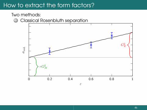
How to extract the form factors?
Two methods:1 Classical Rosenbluth separation
0 0.2 0.4 0.6 0.8 1
σred.
ε
τG2M
G2E
2 ”Super-Rosenbluth separation”: Fit of form factormodels directly to the measured cross sections
Feasible due to fast computers.All data at all Q2 and ε values contribute to the fit, i.e.full kinematical region used, no projection (to specificQ2) needed.Easy fixing of normalization.
Model dependence?
For radii extraction: Needs a fit anyway!Classical Rosenbluth: Extracted GE and GM highlycorrelated! =⇒Error propagation very involved.
46

How to extract the form factors?
Two methods:1 Classical Rosenbluth separation2 ”Super-Rosenbluth separation”: Fit of form factor
models directly to the measured cross sections
Feasible due to fast computers.All data at all Q2 and ε values contribute to the fit, i.e.full kinematical region used, no projection (to specificQ2) needed.Easy fixing of normalization.
Model dependence?
For radii extraction: Needs a fit anyway!Classical Rosenbluth: Extracted GE and GM highlycorrelated! =⇒Error propagation very involved.
47

How to extract the form factors?
Two methods:1 Classical Rosenbluth separation2 ”Super-Rosenbluth separation”: Fit of form factor
models directly to the measured cross sections
Feasible due to fast computers.All data at all Q2 and ε values contribute to the fit, i.e.full kinematical region used, no projection (to specificQ2) needed.Easy fixing of normalization.Model dependence?
For radii extraction: Needs a fit anyway!Classical Rosenbluth: Extracted GE and GM highlycorrelated! =⇒Error propagation very involved.
48

How to extract the form factors?
Two methods:1 Classical Rosenbluth separation2 ”Super-Rosenbluth separation”: Fit of form factor
models directly to the measured cross sections
Feasible due to fast computers.All data at all Q2 and ε values contribute to the fit, i.e.full kinematical region used, no projection (to specificQ2) needed.Easy fixing of normalization.Model dependence?
For radii extraction: Needs a fit anyway!Classical Rosenbluth: Extracted GE and GM highlycorrelated! =⇒Error propagation very involved.
49

Models
Dipole, double DipoleFriedrich / Walcher phenomenological ansatzextended Gari-Krümpelmann (VMD), Lomon et al.Polynomials (+/× dipole)Splines
50
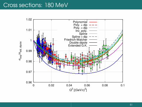
Cross sections: 180 MeV
0.96
0.97
0.98
0.99
1
1.01
1.02
0 0.02 0.04 0.06 0.08 0.1
σe
xp/σ
std
. d
ipo
le
Q2 [(GeV/c)
2]
PolynomialPoly. + dipPoly. × dip
Inv. poly.Spline
Spline × dipFriedrich-Walcher
Double dipoleExtended G.K.
51

Cross sections: 315 MeV
0.95
0.96
0.97
0.98
0.99
1
1.01
1.02
0 0.05 0.1 0.15 0.2 0.25
σe
xp/σ
std
. d
ipo
le
Q2 [(GeV/c)
2]
PolynomialPoly. + dipPoly. × dip
Inv. poly.Spline
Spline × dipFriedrich-Walcher
Double dipoleExtended G.K.
52

Cross sections: 450 MeV
0.95
0.96
0.97
0.98
0.99
1
1.01
1.02
1.03
0 0.05 0.1 0.15 0.2 0.25 0.3 0.35 0.4
σe
xp/σ
std
. d
ipo
le
Q2 [(GeV/c)
2]
PolynomialPoly. + dipPoly. × dip
Inv. poly.Spline
Spline × dipFriedrich-Walcher
Double dipoleExtended G.K.
53

Cross sections: 585 MeV
0.94
0.96
0.98
1
1.02
1.04
1.06
1.08
0 0.1 0.2 0.3 0.4 0.5 0.6
σe
xp/σ
std
. d
ipo
le
Q2 [(GeV/c)
2]
PolynomialPoly. + dipPoly. × dip
Inv. poly.Spline
Spline × dipFriedrich-Walcher
Double dipoleExtended G.K.
54

Cross sections: 720 MeV
0.95
1
1.05
1.1
1.15
0 0.1 0.2 0.3 0.4 0.5 0.6 0.7 0.8
σe
xp/σ
std
. d
ipo
le
Q2 [(GeV/c)
2]
PolynomialPoly. + dipPoly. × dip
Inv. poly.Spline
Spline × dipFriedrich-Walcher
Double dipoleExtended G.K.
55

Cross sections: 855 MeV
0.95
1
1.05
1.1
1.15
1.2
0 0.2 0.4 0.6 0.8 1
σexp/σ
std
. dip
ole
Q2 [(GeV/c)
2]
PolynomialPoly. + dipPoly. × dip
Inv. poly.Spline
Spline × dipFriedrich-Walcher
Double dipoleExtended G.K.
56

GE
0.8
0.85
0.9
0.95
1
1.05
1.1
0 0.2 0.4 0.6 0.8 1
GE/G
std
. dip
ole
Q2 [(GeV/c)
2]
Spline + stat. error + exp. syst. error + theo. syst. errorF.-W. fit
Arrington et al.F.-W. 2003Christy et al.Simon et al.Price et al.
Berger et al.Hanson et al.Borkowski et al.Janssens et al.Murphy et al.
57

GE - low Q2
0.94
0.95
0.96
0.97
0.98
0.99
1
1.01
1.02
0 0.05 0.1 0.15 0.2 0.25 0.3
GE/G
std
. dip
ole
Q2 [(GeV/c)
2]
Spline + stat. error + exp. syst. error + theo. syst. errorF.-W. fit
Arrington et al.F.-W. 2003Christy et al.Simon et al.Price et al.
Berger et al.Hanson et al.Borkowski et al.Janssens et al.Murphy et al.
58

GM
0.94
0.96
0.98
1
1.02
1.04
1.06
1.08
1.1
0 0.2 0.4 0.6 0.8 1
GM
/(µ
pG
std
. dip
ole
)
Q2 [(GeV/c)
2]
Spline + stat. error + exp. syst. error + theo. syst. errorF.-W. fit
Arrington et al.F.-W. 2003Christy et al.Price et al.Berger et al.
Hanson et al.Borkowski et al.Janssens et al.Bosted et al.Bartel et al.
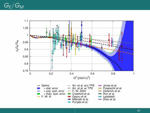
59
GE/GM
0.75
0.8
0.85
0.9
0.95
1
1.05
1.1
0 0.2 0.4 0.6 0.8 1
µpG
E/G
M
Q2 [(GeV/c)
2]
Spline + stat. error + exp. syst. error + theo. syst. errorF.-W. fit
Arr. et al. w/o TPEArr. et al. w/ TPEF.-W. 2003Crawford et al.Gayou et al.Milbrath et al.Punjabi et al.
Jones et al.Pospischil et al.Dieterich et al.Ron et al.(updated)Zhan et al.
60

Inclusion of world data
Extend data base with world data=⇒ Cross check, extend Q2 reach
Take cross sections from Rosenbluthexp’sSidestep unknown error correlation
Update / standardize radiativecorrectionsOne normalization parameter persource (Andivahis: 2)
Two models:
Splines with variable knot spacing=⇒ Adapt knot density to datadensityPadé-Expansion=⇒ Low(er) flexibility, for comparison
L. Andivahis et al.,Phys. Rev. D50, 5491 (1994).
F. Borkowski et al.,Nucl. Phys. B93, 461 (1975).
F. Borkowski et al.,Nucl.Phys. A222, 269 (1974).
P. E. Bosted et al.,Phys. Rev. C 42, 38 (1990).
M. E. Christy et al.,Phys. Rev. C70, 015206 (2004)
M. Goitein et al.,Phys. Rev. D 1, 2449 (1970).
T. Janssens et al.,Phys. Rev. 142, 922 (1966).
J. Litt et al.,Phys. Lett. B31, 40 (1970).
L. E. Price et al.,Phys. Rev. D4, 45 (1971).
I. A. Qattan et al.,Phys. Rev. Lett. 94, 142301 (2005).
S. Rock et al.,Phys. Rev. D 46, 24 (1992).
A. F. Sill et al.,Phys. Rev. D 48, 29 (1993).
G. G. Simon et al.,Nucl. Phys. A 333, 381 (1980).
S. Stein et al.,Phys. Rev. D 12, 1884 (1975).
R. C. Walker et al.,Phys. Rev. D 49, 5671 (1994).
61
Inclusion of world data
Extend data base with world data=⇒ Cross check, extend Q2 reachTake cross sections from Rosenbluthexp’sSidestep unknown error correlation
Update / standardize radiativecorrectionsOne normalization parameter persource (Andivahis: 2)
Two models:
Splines with variable knot spacing=⇒ Adapt knot density to datadensityPadé-Expansion=⇒ Low(er) flexibility, for comparison
L. Andivahis et al.,Phys. Rev. D50, 5491 (1994).
F. Borkowski et al.,Nucl. Phys. B93, 461 (1975).
F. Borkowski et al.,Nucl.Phys. A222, 269 (1974).
P. E. Bosted et al.,Phys. Rev. C 42, 38 (1990).
M. E. Christy et al.,Phys. Rev. C70, 015206 (2004)
M. Goitein et al.,Phys. Rev. D 1, 2449 (1970).
T. Janssens et al.,Phys. Rev. 142, 922 (1966).
J. Litt et al.,Phys. Lett. B31, 40 (1970).
L. E. Price et al.,Phys. Rev. D4, 45 (1971).
I. A. Qattan et al.,Phys. Rev. Lett. 94, 142301 (2005).
S. Rock et al.,Phys. Rev. D 46, 24 (1992).
A. F. Sill et al.,Phys. Rev. D 48, 29 (1993).
G. G. Simon et al.,Nucl. Phys. A 333, 381 (1980).
S. Stein et al.,Phys. Rev. D 12, 1884 (1975).
R. C. Walker et al.,Phys. Rev. D 49, 5671 (1994).
62

Inclusion of world data
Extend data base with world data=⇒ Cross check, extend Q2 reachTake cross sections from Rosenbluthexp’sSidestep unknown error correlation
Update / standardize radiativecorrectionsOne normalization parameter persource (Andivahis: 2)
Two models:
Splines with variable knot spacing=⇒ Adapt knot density to datadensityPadé-Expansion=⇒ Low(er) flexibility, for comparison
L. Andivahis et al.,Phys. Rev. D50, 5491 (1994).
F. Borkowski et al.,Nucl. Phys. B93, 461 (1975).
F. Borkowski et al.,Nucl.Phys. A222, 269 (1974).
P. E. Bosted et al.,Phys. Rev. C 42, 38 (1990).
M. E. Christy et al.,Phys. Rev. C70, 015206 (2004)
M. Goitein et al.,Phys. Rev. D 1, 2449 (1970).
T. Janssens et al.,Phys. Rev. 142, 922 (1966).
J. Litt et al.,Phys. Lett. B31, 40 (1970).
L. E. Price et al.,Phys. Rev. D4, 45 (1971).
I. A. Qattan et al.,Phys. Rev. Lett. 94, 142301 (2005).
S. Rock et al.,Phys. Rev. D 46, 24 (1992).
A. F. Sill et al.,Phys. Rev. D 48, 29 (1993).
G. G. Simon et al.,Nucl. Phys. A 333, 381 (1980).
S. Stein et al.,Phys. Rev. D 12, 1884 (1975).
R. C. Walker et al.,Phys. Rev. D 49, 5671 (1994).
63

It works!
-8%
-6%
-4%
-2%
0%
+2%
+4%
+6%
+8%
0.01 0.1 1 10
∆σ
Q2[(GeV/c)2]
64
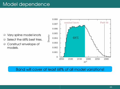
Model dependence
Vary spline model knots
Select the 68% best tries.
Construct envelope ofmodels.
0
0.001
0.002
0.003
0.004
0.005
0.006
0.007
0.008
2050 2100 2150 2200 2250 2300
Den
sity
M2
nominal knots Padé fit
68%
Band will cover at least 68% of all model variations!
65

Form factor ratio GE/GM
-0.5
0
0.5
1
1.5
0 2 4 6 8 10
µpG
E/G
M
Q2[(GeV/c)2]
Difference between polarization data andRosenbluth dataAdd polarization data as a constraint to the fit:=⇒ ∆χ2 = 216 for 67 new data points!
66
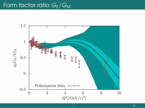
Form factor ratio GE/GM
-0.5
0
0.5
1
1.5
0 2 4 6 8 10
µpG
E/G
M
Q2[(GeV/c)2]
Polarization data
Difference between polarization data andRosenbluth dataAdd polarization data as a constraint to the fit:=⇒ ∆χ2 = 216 for 67 new data points!
67

Form factor ratio GE/GM
-0.5
0
0.5
1
1.5
0 2 4 6 8 10
µpG
E/G
M
Q2[(GeV/c)2]
Polarization data
Difference between polarization data andRosenbluth dataAdd polarization data as a constraint to the fit:=⇒ ∆χ2 = 216 for 67 new data points!
68

Two Photon Exchange - A parametrisation
Available data is sparseMostly Q2 dependenceFew data on ε dependence
Only possible to fit simple modelIn addition to Feshbach Coulomb-correction!
δ = a · (1− ε) · log(
1 + b ·Q2)
69

Two Photon Exchange - A parametrisation
Available data is sparseMostly Q2 dependenceFew data on ε dependenceOnly possible to fit simple modelIn addition to Feshbach Coulomb-correction!
δ = a · (1− ε) · log(
1 + b ·Q2)
70
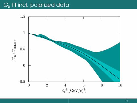
GE fit incl. polarized data
-0.5
0
0.5
1
1.5
0 2 4 6 8 10
GE/G
std.dip.
Q2[(GeV/c)2]
71
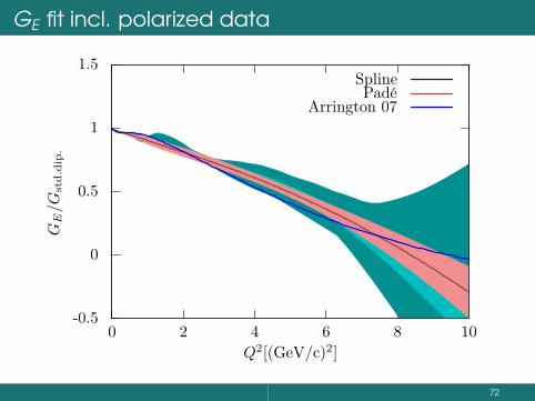
GE fit incl. polarized data
-0.5
0
0.5
1
1.5
0 2 4 6 8 10
GE/G
std.dip.
Q2[(GeV/c)2]
SplinePadé
Arrington 07
72
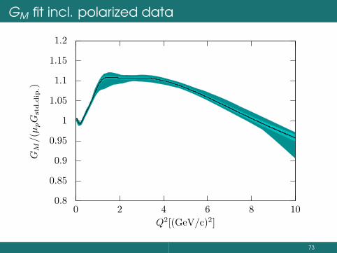
GM fit incl. polarized data
0.8
0.85
0.9
0.95
1
1.05
1.1
1.15
1.2
0 2 4 6 8 10
GM/(µpG
std.dip.)
Q2[(GeV/c)2]
73

GM fit incl. polarized data
0.8
0.85
0.9
0.95
1
1.05
1.1
1.15
1.2
0 2 4 6 8 10
GM/(µpG
std.dip.)
Q2[(GeV/c)2]
SplinePadé
Arrington 07
74

GE/GM fit incl. polarized data
-0.5
0
0.5
1
1.5
0 2 4 6 8 10
µpG
E/G
M
Q2[(GeV/c)2]
75

GE/GM fit incl. polarized data
-0.5
0
0.5
1
1.5
0 2 4 6 8 10
µpG
E/G
M
Q2[(GeV/c)2]
SplinePadé
Arrington 07Polarization data
76

Low Q2
Q2Q2
Q2
77

Radius
0.740.760.780.8
0.820.840.860.880.9
0.92
<r E
>[fm
]
CO
DAT
A’0
2
Mel
niko
v’0
0
Ude
m’9
7
Blu
nden
’05
Sick
’03
Ros
enfe
lder
’00
Mer
gell
’96
Won
g’9
4
Esch
rich
’01
McC
ord
’91
Sim
on’8
0
Bor
kow
ski’
75
Aki
mov
’72
Frer
ejac
que
’66
Han
d’6
3
78

Electric and magnetic radius
Final result from flexible models
⟨r2E
⟩ 12
=0.879± 0.005stat. ± 0.004syst. ± 0.002model ± 0.004group fm,⟨r2M
⟩ 12
=0.777± 0.013stat. ± 0.009syst. ± 0.005model ± 0.002group fm.
Results with world data ⟨r2E
⟩ 12
⟨r2M
⟩ 12
+ Rosenbluth data 0.878 0.772+Rosenbluth and Polarization data 0.878 0.769
(Eur.Phys.J. D33 (2005) 23-27: Zemach and magneticradius of the proton from the hyperfine splitting inhydrogen: 0.778(29) fm)
79

Electric and magnetic radius
Final result from flexible models
⟨r2E
⟩ 12
=0.879± 0.005stat. ± 0.004syst. ± 0.002model ± 0.004group fm,⟨r2M
⟩ 12
=0.777± 0.013stat. ± 0.009syst. ± 0.005model ± 0.002group fm.
Results with world data ⟨r2E
⟩ 12
⟨r2M
⟩ 12
+ Rosenbluth data 0.878 0.772+Rosenbluth and Polarization data 0.878 0.769
(Eur.Phys.J. D33 (2005) 23-27: Zemach and magneticradius of the proton from the hyperfine splitting inhydrogen: 0.778(29) fm)
80

Lamb Shift: muonic Hydrogen
81

Timeline of proton radius results (current)
0.740.760.780.8
0.820.840.860.880.9
0.92
<r E
>[fm
]
CO
DAT
A’0
6
CO
DAT
A’0
2
Mel
niko
v’0
0U
dem
’97
Blu
nden
’05
Sick
’03
Ros
enfe
lder
’00
Mer
gell
’96
Won
g’9
4
Esch
rich
’01
McC
ord
’91
Sim
on’8
0B
orko
wsk
i’75
Aki
mov
’72
Frer
ejac
que
’66
Han
d’6
3
Bel
ushk
in’0
6
Ber
naue
r’1
0Poh
l’10
Ant
ogni
ni’1
3
Paz
’10
Lore
nz’1
2Zh
an’1
1
82

Puzzle!
[fm]ch
Proton charge radius R0.83 0.84 0.85 0.86 0.87 0.88 0.89 0.9
H spectroscopy
scatt. Mainz
scatt. JLab
p 2010µ
p 2013µ electron avg.
σ7.9
Many ideasSome disprovedNone acceptedNeed more data
83

New Data!
Hyperfine measurements:
Heavier Nucleielectronic Hydrogen
Radius from scattering
Deuterium (Mainz)Proton: ISR (Mainz), Smallangle scattering (JLab)
Form factors
Low Q2 polarized (JLab)MAMI-C (1.6 GeV)High precision crosssection at high Q2 (JLab)
Two photon exchange
VEPP-3JLabOlympus
Interesting at all scales
Precision measurements drive precise understanding(through puzzles!)
RadiusTwo photon exchange
More data will come84