arX

iv:h

ep-p

h/03

0508

5v1

8 M

ay 2

003

RHIC Spin Note

May 2003

Proton-carbon CNI polarimetry and the spin-dependence of the

Pomeron

T.L. Trueman 1

Physics Department, Brookhaven National Laboratory, Upton, NY 11973

Abstract

Recent polarized proton experiments at Brookhaven National Laboratory are used as a basis

for a model of the energy dependence of the analyzing power of proton-carbon elastic scattering.

In addition to their practical value for polarimetry, the results of this analysis give constraints

on the size of the Pomeron spin-flip coupling as well as information on the f2 and ω spin-flip

couplings.

1This manuscript has been authored under contract number DE-AC02-76CH00016 with the U.S. Department ofEnergy. Accordingly, the U.S. Government retains a non-exclusive, royalty-free license to publish or reproduce thepublished form of this contribution, or allow others to do so, for U.S. Government purposes.

1

During the past three years experiments have been carried out at Brookhaven National Labo-

ratory, at the AGS with proton beam momentum of 21.7 GeV/c and at RHIC with beam mo-

menta of 24 GeV/c and 100 GeV/c, to measure the single-spin asymmetry for elastic scattering

of transversely polarized proton beams off (fixed) carbon targets. The principal goal of these ex-

periments is to obtain a calibrated polarimeter based on elastic pC scattering in the CNI region,

i.e. |t| ≤ 0.05 (GeV/c)2. In outline, the procedure to be used is to begin with an AGS beam of

known polarization, and to measure the analyzing power AN (t) near the RHIC injection energy. In

the CNI region the analyzing power is expected to be a few percent which, coupled with the large

rate, makes it well-suited to be a practical polarimeter. The ultimate goal is to have a sufficently

precise calibration to make the desired 5% measurement of the polarization P . (As we will see

the current experimental errors are too large to reach this level of absolute accuracy, though the

relative errors are quite small.. This should improve soon as further experiments are carried out,

but it may ultimately require the use of a polarized hydrogen gas jet target to reach the required

level of 5% absolute). This AGS experiment is referred to as E950. See [1] for a description of the

experiment and the results. The next step is to measure the asymmetry after transfer of the beam

into RHIC with a setup the same as or similar to the one in the AGS. The energy at this point is a

little higher than where the calibration is made, but the analyzing power is not expected to change

enough that significant additional uncertainty is introduced into the measurement of P .

The difficult and as yet not solved problem has to do with the polarization at higher

energy in RHIC. It would be nice to believe that the polarization is not reduced during the RHIC

acceleration, but this is not really known, and it would be good to have some theoretical guidance

as to what sort of energy dependence the CNI analyzing power is expected to have. The central

goal of this paper is to present a plausible model, based on Regge phenomenology, to calculate

AN (t) at higher energy assuming only that a calibrated measurement can be made at injection.

The model, as utilized here, has as spin-off some interesting theoretical results. In particular, the

question of the spin-dependence ot the Pomeron coupling to the proton has been studied for many

years with still no firm conclusion. (See [2] for an extensive discussion of this issue.) It is generally

known to be small, less than 10-15%, but not better known than that. The analyzing power is very

sensitive to this coupling, as we will see, and so even low energy data, like that from the AGS, can

give us very good information about this coupling.

1

The model we will adopt uses three Reggeons, the Pomeron P and two Regge poles, f2 and

ω. Because carbon is an isosinglet none of the I = 1 Regge poles like the ρ or a2 can enter, but

because they are known to make small contributions to the elastic, non-flip amplitudes [5] we can

use the fits for unpolarized pp and p̄p elastic scattering that have been carried out over an extensive

energy range. [3, 4] (To carry over our results to pp spin-flip will require important corrections

because ρ and a2 spin-flip couplings are known to be strong [5, 6]. See Section 5, below.)

We will begin by discussing the determination of AN (t) from the data obtained in E950. This

analyzing power will then be applied to determine the polarization in RHIC from the asymmetry

measured there at 24 GeV/c. Next we will describe how the 3-Reggeon model is extended from

elastic non-flip scattering to spin-flip scattering and will examine what we can say about the model

just based on the E950 results. We will then examine the RHIC data taken at 100 GeV/c and will

see that, without knowing the polarization in RHIC at that energy, all the parameters of our model

can be determined by measuring, in addition to the E950 results, the polarization-independent

“shape” of the asymmetry distribution in the CNI region. This being done, we can calculate P at

100 GeV/c without further data fitting. The model predicts the analyzing power at any energy,

and we will examine this a little by checking on the variation between 21.7 GeV/c and 24 GeV/c

and predicting the AN (t) at 250 GeV/c. The prediction for the I = 0 part of the pp analyzing

power through the RHIC colliding beam range will be given and some model dependence examined.

We will attempt to include the ρ and a2 in our analysis in order to apply our results to pp

scattering . The data from FermiLab E704 [7] will be used to make tentative predictions for pp

polarimetry at high energy.

The effects we are looking at are rather small and the errors involved in the analysis are

significant and generally correlated. Therefore we devote the last section of the paper to a careful

analysis of the errors of the Reggeon spin-flip couplings determined earlier in the paper. The

implications for the errors on the analyzing power as a function of energy are also worked out.

2

The formula we use for the pC analyzing power was derived by Kopeliovich and the author [8].

The approximations that go into the formula are discussed in that paper, and it is believed to be

quite reliable over the small t-range involved in the CNI experiments. A particularly transparent

2

way to write it is

AN (t, τ)

AN (t, 0)= 1− 2

κRe[ τ(s)] +

2

κIm[ τ(s)]f(t), (1)

with

f(t) =(

(1 + ρ2pC(t))(t/tc)(FhC(t)/F

emC (t))− ρpC(t)− δpC(t)

)

/(1− ρpC(t)δpC(t)) (2)

τ(s) denotes the hadronic spin-flip parameter for the scattering. It will be defined precisely below.

AN (t, τ) is the analyzing power in question and AN (t, 0) is “pure” CNI, the analyzing power in the

absence of hadronic spin-flip. F emC (t) is the electromagnetic form-factor and F h

C(t) is the hadronic

form-factor for carbon; these are calculated in [8]. κ = 1.79, tc = −8πZα/σpCtot and ρpC(t) denotes

the ratio of real to imaginary parts of the pC amplitude (It depends on t even if ρ for pp does not,

as assumed in the derivation of Eq.1; it is also calculated in [8].) δpC(t) denotes the Bethe phase

[9] for proton-carbon scattering; it is important only at the smallest values of |t|, smaller than for

which data so far exists, but we carry it along anyway. We have neglected in writing Eq.1 the

dependence of the differential cross-section on τ which is insignificant when τ is small, in the range

we anticipate. τ(s) is defined by

g5(s, t) = τ(s)

√−t

mg0(s, t) (3)

g0(s, t) and g5(s, t) denote, respectively, the spin independent and spin-flip pC elastic amplitudes.

m denotes the proton mass. One of the main results of [8] is that τ(s) is equal to the I = 0 part

of the corresponding spin-flip factor for pp scattering. It is, in general, complex and depends on

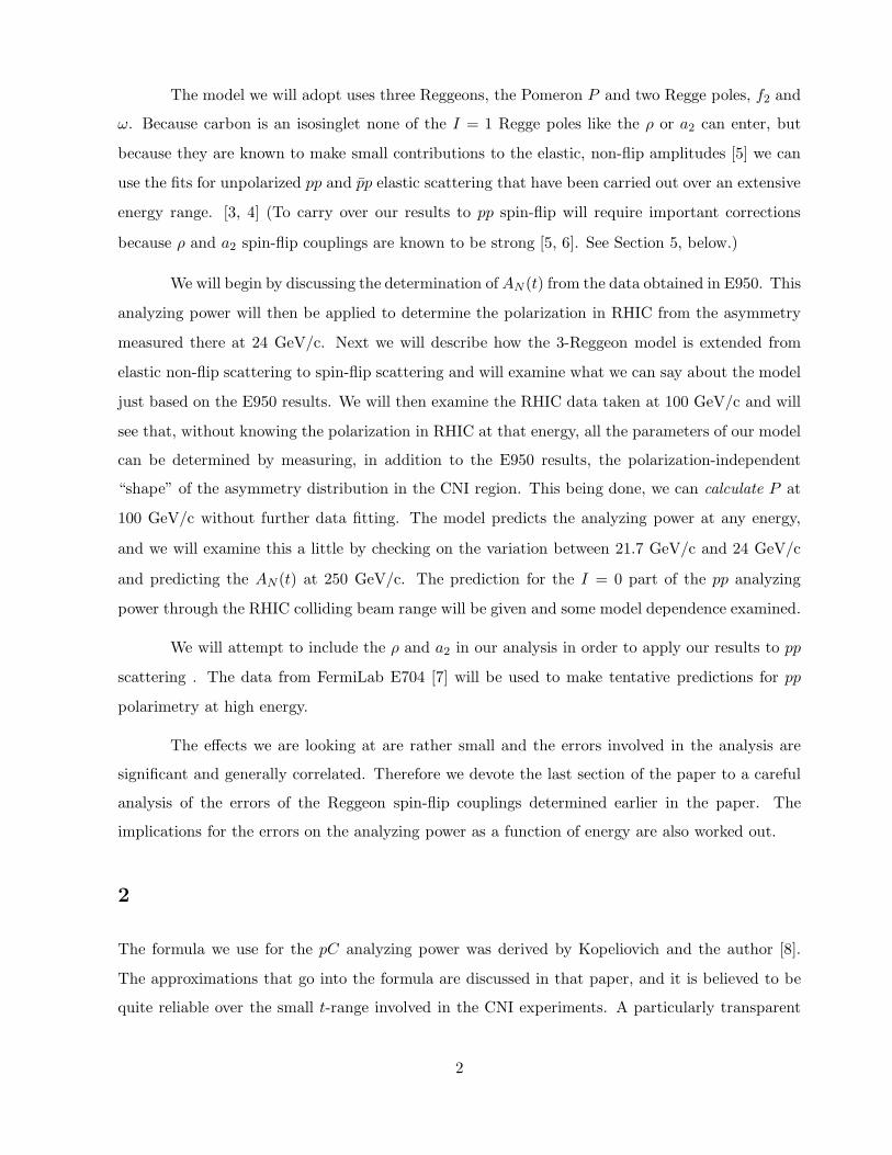
s in an unknown way, but its t-dependence can be neglected over this small range of t. All the

important t-dependence of Eq.1 comes from the variation of the form factors and of ρpC . The

resulting dependence of f(t) is shown in Fig.1.

It is important to note that this formula is given in terms of τ(s) rather than

rpC5

(s, t) = τ(s)(i+ ρpC(s, t))

which is sometimes used. This has the advantage that, by the theorem of [8], τ is independent of t

while rpC5

has t-dependence inherited from ρpC .

3

0.01 0.02 0.03 0.04 0.05

5

10

15

20

f(t)

-t

Figure 1: The t-dependent coefficient in the second term of Eq. 1.

The E950 group fit their data in [1] and determined values for rpC5

. We could simply use

their results, but because the propagation of errors to our later results is important, we have done a

linear regression analysis of our own and calculated the error matrix for Re(τ) and Im(τ). The data

we fit is given in their Table 1 and we used the errors given there to determine the weights in the

regression analysis. These errors include an approximately 12% error in the AGS beam polarization.

(We have followed E950 in adding the errors linearly; perhaps this should be reexamined.) The

results of this fits gives

τ = (−0.214 ± 0.236) − (0.054 ± 0.015)i (4)

The very large error on the real part of τ results from a modest error on the first term in

Eq.1 of about 25%,. The error in the imaginary part is also about 20%. These errors are too large

for the job of doing a 5% absolute polarization measurement, and they will follow us through all

of this work.

There are additonal errors in these numbers because of unassessed errors in the parametriza-

tion of Eq.1. In particular, the value of ρpC used is calculated. It would be good to measure it.

The same is true of the pC differential cross section which determines F hC(t). The error in our

calculation of these quantities is probably small, but it depends on, as input, the poorly known

value of ρ for pp and pn at 21.7 GeV/c. This will need to be addressed when the other errors are

reduced. (The values published in [1] agree within errors with Eq.(4).)

4

0.015 0.02 0.025 0.03 0.035 0.04

-0.4

-0.2

0.2

0.4

0.6

0.8

AN(τ)

AN(0)

−t

Figure 2: The error bands for the fit of E950 data to Eq.1

The results of the fit are shown in Fig.2 and Fig.3, first showing the error bands on the

regression analysis and second showing the AN (t) compared to the data. The error matrix for

0.01 0.02 0.03 0.04 0.05

0.01

0.02

0.03

0.04

AN(τ)

-t

Figure 3: Fit of analyzing power using τ = −0.214 − 0.054i to the data of E950

Re(τ) and Im(τ) is given by

σ2(21.7) =

(

0.0559 0.003320.00332 0.000213

)

(5)

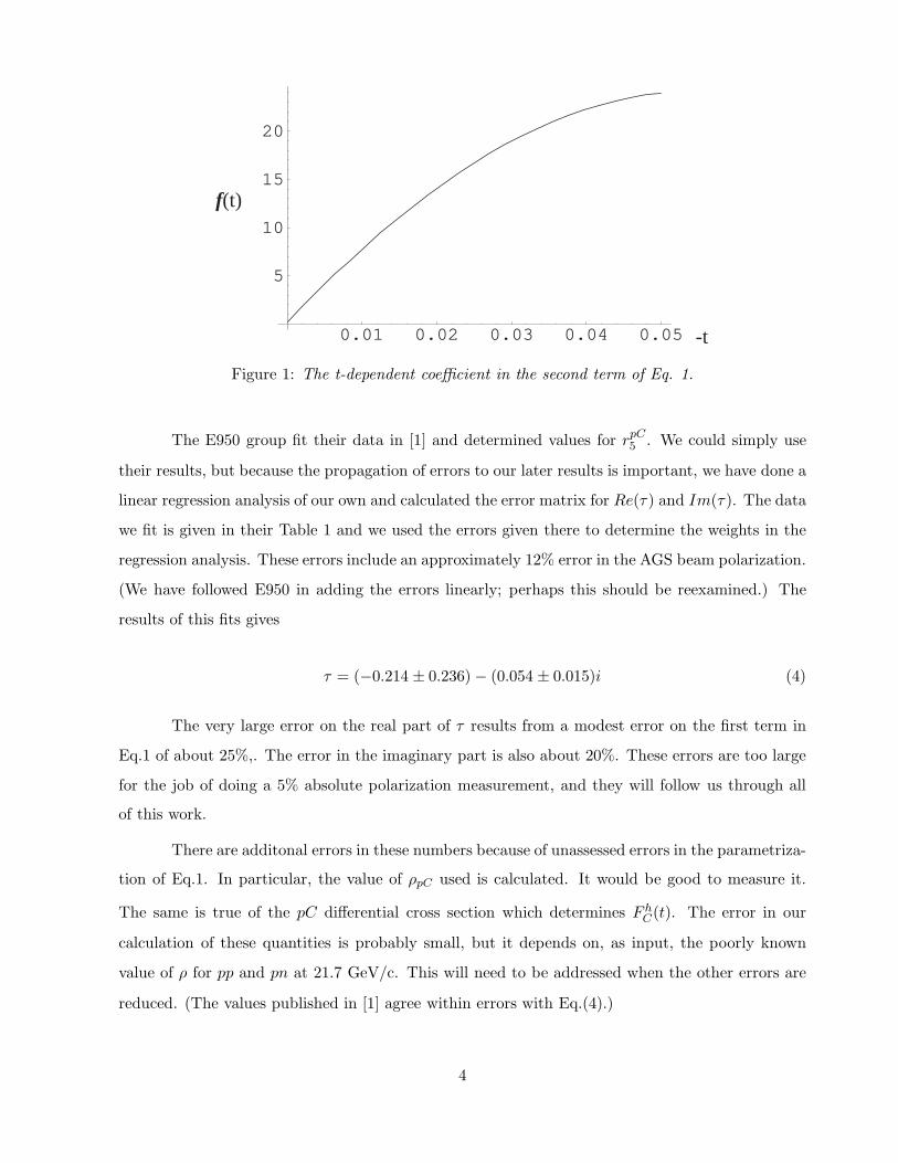
and the corresponding 68.3% confidence level ellipse for the fit parameters (not the τ ’s) is shown

in Fig.4

It is important to bear in mind that if one attempts to fit the data using an incorrect

5

Re(τ)

Im(τ)

-0.4 -0.3 -0.2 -0.1

-0.065

-0.055

-0.05

-0.045

-0.04

Figure 4: The 1σ error ellipse for the fit to E950 data

assumption regarding the polarization, call it P ′, one will obtain a perfectly good fit with exactly

the same χ2 as the correct one; one will simply determine values of the fit parameters which scale

as

1− 2

κRe(τ ′) =

P

P ′

(

1− 2

κRe(τ)

)

,

Im(τ ′) =P

P ′Im(τ). (6)

3

As a first application of these results, let us use the analyzing power just determined at 21.7 GeV/c

to determine the polarization of the beam in RHIC after injection at 24 GeV/c. To do this we

assume that AN (t) doesn’t change significantly over this small energy range. We will return to this

question after we develop a model for the energy dependence. We will use the preliminary data for

the raw asymmetry ǫ(t) which does not depend on any knowledge of the polarization of the beam,

as presented at Prague in July 2002 [10] and at Spin 2002 [11]. The data for ǫ(t) with errors e(t)

are given in Table 1. The errors given assume that the systematic errors are equal to the statistical

errors and they are combined in quadrature. (I thank D. Svirida for this information.) Evidently,

these errors do not contain a contribution from the polarization because this is the raw asymmetry,

not AN . (The values of AN given in those references are calculated assuming P = 0.27 and so if

6

one fits AN instead of ǫ(t) one will obtain values for τ scaled as mentioned at the end of the last

section. These turn out to be very different than the values in the E950 fit.)

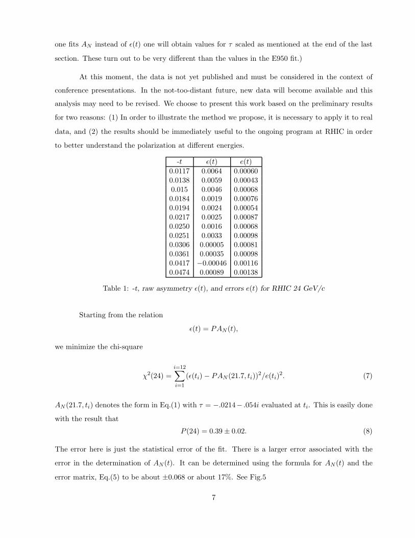
At this moment, the data is not yet published and must be considered in the context of

conference presentations. In the not-too-distant future, new data will become available and this

analysis may need to be revised. We choose to present this work based on the preliminary results

for two reasons: (1) In order to illustrate the method we propose, it is necessary to apply it to real

data, and (2) the results should be immediately useful to the ongoing program at RHIC in order

to better understand the polarization at different energies.

-t ǫ(t) e(t)

0.0117 0.0064 0.000600.0138 0.0059 0.000430.015 0.0046 0.000680.0184 0.0019 0.000760.0194 0.0024 0.000540.0217 0.0025 0.000870.0250 0.0016 0.000680.0251 0.0033 0.000980.0306 0.00005 0.000810.0361 0.00035 0.000980.0417 −0.00046 0.001160.0474 0.00089 0.00138

Table 1: -t, raw asymmetry ǫ(t), and errors e(t) for RHIC 24 GeV/c

Starting from the relation

ǫ(t) = PAN (t),

we minimize the chi-square

χ2(24) =

i=12∑

i=1

(ǫ(ti)− PAN (21.7, ti))2/e(ti)

2. (7)

AN (21.7, ti) denotes the form in Eq.(1) with τ = −.0214− .054i evaluated at ti. This is easily done

with the result that

P (24) = 0.39 ± 0.02. (8)

The error here is just the statistical error of the fit. There is a larger error associated with the

error in the determination of AN (t). It can be determined using the formula for AN (t) and the

error matrix, Eq.(5) to be about ±0.068 or about 17%. See Fig.5

7

0.01 0.02 0.03 0.04 0.05

0.003

0.004

0.005

0.006

0.007

0.008

∆ΑΝ(t)

−t

Figure 5: The uncertainty in the analyzing power predicted at 24 GeV/c

Now using the E950 value of τ and this polarization we plot together the expected asym-

metry along with the RHIC 24 GeV/c data, Fig.6. The fit is reasonable with χ2 = 1.5 per dof.

0.01 0.02 0.03 0.04 0.05

0.0025

0.005

0.0075

0.01

0.0125

0.015

P=0.39

-t

ε(t)

Figure 6: Raw asymmetry at 24 GeV/c as measured and as predicted by E950 analyzing power withP=0.39

8

4

Can we say anything about the energy dependence of AN (t) based on the the E950 or RHIC 24

data alone? The simplest plausible Regge model to describe the energy dependence has three

Regge poles: the Pomeron, the f2 and the ω. There have been at least two groups [3, 4] which have

produced fits to the extensive data for pp and p̄p elastic scattering over an enormous energy range

which includes almost all of the RHIC energy range. The lowest energy, which includes our starting

point, is marginal to the fits. Nevertheless we will use these models as a basis for our own model. In

these fits the f2 and the ω are always treated as simple Regge poles, but the more complex nature

of the Pomeron is taken into account by allowing it to be alternatively a simple pole a little above

J = 1 , or multiple poles at J = 1 in order to produce single or double logarithms in the asymptotic

energy dependence of the total cross section. For this work we have chosen two representitive fits

from [3], a simple pole at 1.0933 or a multiple pole at 1 designed to give a log-square growth. We

will work through the first case first and then indicate how the second differs from it.

We begin with the parametrization of pp elastic scattering given by Cudell et al [3], though

one might do the same thing using other parametrizations such as that of Block et al [4]. Since it

is known that the elastic, non-flip scattering is overwhelmingly I = 0 exchange, even at 24 GeV/c

[12], we will assume the Regge couplings that they determine are for the I = 0 families and so

directly applicable to pC scattering. The form they assume for the forward amplitude is

g0(s, 0) = gP (s) + gf (s) + gω(s) (9)

with

gP (s) = −Xsǫ(cotπ

2(1 + ǫ)− i), (10)

gf (s) = −Y s−η(cotπ

2(1− η)− i),

gω(s) = −Y ′s−η′(tanπ

2(1− η′) + i)

normalized that Im(g0(s)) = σtot(s). The values of the parameters given by them are

ǫ = 0.0933, η = 0.357, η′ = 0.560, (11)

X = 18.79, Y = 63.0, Y ′ = 36.2,

9

with X,Y, Y ′ in mb.

Our model assumes that the spin-flip pp I = 0 exchange amplitude g5(s, t) is given by

g5(s, t) = τ(s)

√−t

mg0(s, t) (12)

=

√−t

m{τP gP (s) + τf gf (s) + τω gω(s)}.

where τ(s) depends on energy but not on t over the CNI range. It is in general neither real nor

constant in s and is given by

τ(s) = {τP gP (s) + τf gf (s) + τω gω(s)}/g0(s, 0) (13)

where the τi’s are energy-independent, real constants. The phases of the amplitudes come only

from the energy dependence as given in Eq.(10). This is the key assumption from Regge theory

which we need: as a result the real and imaginary parts of τ(s) are given at each energy in terms

of the three real constants τP , τf and τω.

Since from E950 we can determine only two real parameters, it is plain that we can not fix

this model completely. The best we can do is obtain a relation between the three spin flip couplings;

for example, in Fig.7 we plot τf and τω as constrained by the values of Eq.(4).

The recent runs at RHIC have also provided data at 100 GeV/c. The polarization is not

known there, so is it possible to obtain useful information from it? The answer is yes: if the

asymmetry is described by the CNI formula, which is our fundamental assumption, then a fit to

the raw asymmetry will determine (1− 2

κRe[τ(100)])P (100) and 2

κIm[τ(100)]P (100). (In this and

the following sections we will write the argument of the shape S and τ as the lab momentum rather

than the corresponding s. When we briefly discuss colliding beams, we will revert to s, but there

should not be any confusion.) Thus the “shape” S of the distribution

S(pL) =Im[τ(pL)]

κ/2−Re[τ(pl)](14)

can be determined at any energy without knowing P . Now once we have the three quantities,

Re[τ(21.7)], Im[τ(21.7)] and S(100) we have three linear equations in τP , τF and τω and can deter-

10

-0.4 -0.2 0.2 0.4

-1.5

-1

-0.5

0.5

1

1.5 τω

τf

τP

Figure 7: Relations between the three Regge spinflip coupling based on E950 results alone

mine them all. This then will give us τ(pL) at pL = 100 GeV/c and thereby we can calculate the

polarization P (100). We will now go through this process.

Using data from the same sources as used at 24 GeV/c [10, 11],

-t ǫ(t) e(t)

0.0117 0.0036 0.000550.0138 0.0029 0.000470.015 0.0034 0.000600.0184 0.0018 0.000690.0194 0.0014 0.000580.0217 0.0025 0.000870.0249 −0.0004 0.000720.0251 0.0009 0.000850.0306 −0.0010 0.000720.0360 0.0010 0.000910.0416 0.0013 0.001160.0473 −0.003 0.00146

Table 2: -t, raw asymmetry ǫ(t), and errors e(t) for RHIC 100 GeV/c

We then fit this as in Section 2 to the formula in Eq.(1) with the right hand side multiplied

by the unknown P (100). There is a small calculable energy dependence to f(t), and it is taken into

11

account in the fit. The result of the regression is

P (100)(1 − 2

κRe[τ(100)]) = 0.263 (15)

P (100)2

κIm[τ(100)] = −0.0137.

Combining these together we get for the shape of the distribution

S(100) = −0.0137

0.263= −0.052 (16)

By using Eq.(4) the value of τ(21.7) as determined in E950 in terms of the Regge spin-flip couplings

via Eq.(13) and in the same way express S(100) in term of the Regge spin-flip couplings via τ(100)

and Eq.(13), we have three equations to solve with the result

τP = −0.02 (17)

τf = −0.43

τω = 0.03

There are significant errors in these determinations and we will return to them in the next section.

These results allow us to calculate τ(s) at any higher energy. (The model as it stands, is

not really suitable for going to lower energy because lower lying Regge poles will rapidly beome

important. Thanks to Boris Kopeliovich for emphasizing this limitation [5], [6].) Fig. 8 shows the

pL dependence of the real and imaginary parts of τ over the RHIC fixed target range. While the

spin-flip couplings are evidently becoming smaller with increasing energy, there remains significant

hadronic spin-flip at the top energy.

We will use these results first for τ(100) and thereby determine the polarization at 100

GeV/c, P (100). From Eq.(13) we find

τ(100) = −0.130 − 0.053i (18)

With κ/2 − Re[τ(100)] and/or Im[τ(100)], we can use the measured values of P (100)(κ/2 −

Re[τ(100)]) and/or P (100)Im[τ(100)] to quickly determine P (100) = 0.23. Alternatively, as in

Section 3, we can fit the 12 measured asymmetry values to AN using Eq.(18). Then minimizing

the χ2 as in Eq.(7) we find

P (100) = 0.23 ± 0.02, (19)

12

50 100 150 200 250

-0.25

-0.225

-0.175

-0.15

-0.125

-0.1

Im(τ)

Re(τ)

pL

pL

50 100 150 200 250

-0.055

-0.045

-0.04

Figure 8: Predicted s-dependence of τ

again the error is just the statistical error of this fit. In Fig.9 we show the raw asymmetry measured

at 100 GeV/c plotted with the prediction using Eq.(18) and this value of P . The agreement is

reasonable, with χ2 about 1.5/dof, about the same as the fit at 24 GeV/c. This is rather nice

support for our approach.

Given that P (24) was found to be 0.39, the value found for P (100) is surprisingly small.

There seem to be three possiblilities to explain this: (1) There could be significant depolarization

in the RHIC acceleration to 100 GeV/c. This is not expected, but this may be a signal of a problem

in the acceleration. (2) The model used for energy dependence could be wrong. This seems very

likely in its details, but if one compares the raw asymmetries at 24 and 100 GeV/c, one sees that

a very large drop in the analyzing power–nearly a factor of 2 from 24 to 100 GeV/c is required if

P remained constant. Of course, there might be a problem with the data at the smallest |t|, but itis not suggested by the errors assigned.

In Section 3 we determined P (24) by assuming that τ(24) is the same as τ(21.7) determined

13

0.01 0.02 0.03 0.04 0.05

-0.002

0.002

0.004

0.006

0.008

-t

ε(t)

Figure 9: Raw asymmetry at 100 GeV/c predicted by model τ(100) and polarization predicted to be0.23

by E950. Now we have a prediction for τ(24) and it is a little different:

τ(24) = −0.207 − 0.055i. (20)

We have checked its significance in determining P via Eq.(7) and find the best fit at P = 0.41±0.02,

slightly different but certainly well within errors. (Remember that the result of the fits at 24 GeV/c

were not used in the energy dependence calculations, so this is another check, although not a very

strong one.)

In the near future it is hoped to have a polarized proton run at RHIC at pL = 250 GeV/c.

The predicted analyzing power is shown in Fig.10. It is a little larger and has a slightly different

shape from the 21.7 GeV determination. For clarity we also show in that figure the ratio of predicted

to pure CNI analyzing power. This shows that the hadronic spin-flip must be taken into account

in AN even at the highest RHIC beam energy on a fixed target.

As mentioned earlier, we also examined the behavior of a Cudell et al [3] fit with a log-

squared asymptotic behaviour for the Pomeron. The fit we chose to look at has the Pomeron form

replaced by

gP (s) = i(A+B log2 s) + πB log s, (21)

s in units of GeV2. The Regge pole forms are unchanged, but the associated parameters are

somewhat different:

A = 25.29, B = 0.227, η = 0.341, η′ = 0.558, (22)

Y = 52.6, Y ′ = 36.0,

14

0.01 0.02 0.03 0.04 0.05

0.01

0.02

0.03

0.04

AN(τ)AN(0)

AN(τ)

-t

-t0.01 0.02 0.03 0.04 0.05

0.2

0.4

0.6

0.8

1

Figure 10: Analyzing power predicted for 250 GeV/c pC scattering, and its ratio to the pure CNIanalyzing power at 250 GeV/c

with A,B, Y, Y ′ in mb. The spin-flip parameters associated with this form for the unpolarized

amplitudes are found to be, in the same way as for the 3-pole model

τ ′P = −0.02

τ ′F = −0.49

τ ′ω = 0.02. (23)

These numbers are very similar to those found for the three pole model but not really directly

comparable because the models are, in principle, quite different. They lead to very little difference

in the model preditions. We can accentuate the difference by looking at the very high energy

behavior where the difference between the power and the log’s should be greatest, so in Fig.11 we

show the behaviour of Re[τ ] and Im[τ ] over the full RHIC colliding beam energy range. (Note that

here the x-axis is the s axis.) The difference remains tiny over the entire range. In either case the

15

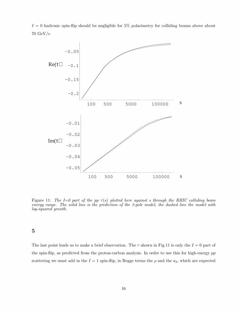
I = 0 hadronic spin-flip should be negligible for 5% polarimetry for colliding beams above about

70 GeV/c.

100 500 5000 100000

-0.2

-0.15

-0.1

-0.05

Re(τ)

Im(τ)

s

s100 500 5000 100000

-0.05

-0.04

-0.03

-0.02

-0.01

Figure 11: The I=0 part of the pp τ(s) plotted here against s through the RHIC colliding beamenergy range. The solid line is the prediction of the 3-pole model, the dashed line the model withlog-squared growth.

5

The last point leads us to make a brief observation. The τ shown in Fig.11 is only the I = 0 part of

the spin-flip, as predicted from the proton-carbon analysis. In order to use this for high-energy pp

scattering we must add in the I = 1 spin-flip, in Regge terms the ρ and the a2, which are expected

16

to be quite large [5]. If we fit the E704 data [7, 2] we find

τ(E704) = 0.2 ± 0.2 + 0.024i ± 0.020i

to be compared with our prediction of the I = 0 part at pL = 200GeV/c

τ0(200) = −0.10− 0.046i.

Even with the very large error on the E704 result, these numbers are incompatible. The difference

can be naturally explained by adding in large I = 1 spin-flip contributions which are absent in

the pC scattering but are known to be important at lower energy in pp scattering [5, 6]. If we

assume that the ρ and a2 have the same Regge behaviour as the ω and the f2, respectively, we can

determine the C = −1 and the C = +1 combined I = 0 and I = 1 Regge flips to be,

τ(C = −) = −2.10

and

τ(C = +) = 0.69.

The relation of these numbers to the ρ and a2 couplings requires more study. However, just with

these numbers and the value we have determined for τP we can calculate the values of the proton

spin-flip expected at high RHIC colliding beam energy, and we find τpp(702) = 0.04 + 0.025i and

τpp(5002) = −.01 + 0.006i so the hadronic spin-flip will have little effect on AN in the CNI region

at the highest energies.

6

Finally, we would like to make some comments on how well the Regge parameters are determined

in this model and using this data, especially on the question of the Pomeron spin-flip coupling.

Starting from the error matrix for τ(21.7) and error on S(100), which requires the error matrix for

τ(100) we can easly propagate the errors to an error matrix of the I = 0 Regge spin-flip factors.

For completeness we give the error matrix for τ(100) determined by our fit, and assuming the

polarization P (100) = 0.23:

σ2(100) =

(

0.0164 0.00120.0012 0.0001

)

. (24)

17

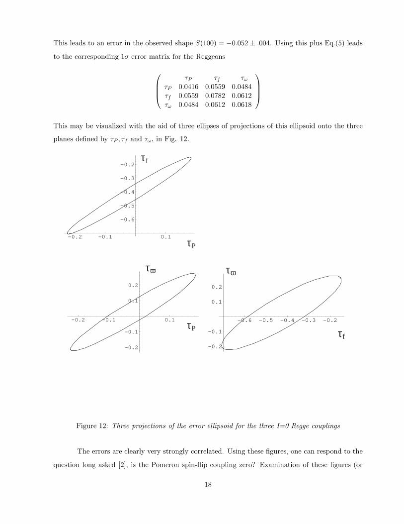
This leads to an error in the observed shape S(100) = −0.052 ± .004. Using this plus Eq.(5) leads

to the corresponding 1σ error matrix for the Reggeons

τP τf τωτP 0.0416 0.0559 0.0484τf 0.0559 0.0782 0.0612τω 0.0484 0.0612 0.0618

This may be visualized with the aid of three ellipses of projections of this ellipsoid onto the three

planes defined by τP , τf and τω, in Fig. 12.

τP

τP

τω τω

τf

-0.2 -0.1 0.1

-0.2

-0.1

0.1

0.2

-0.6 -0.5 -0.4 -0.3 -0.2

-0.2

-0.1

0.1

0.2

-0.2 -0.1 0.1

-0.6

-0.5

-0.4

-0.3

-0.2

τf

Figure 12: Three projections of the error ellipsoid for the three I=0 Regge couplings

The errors are clearly very strongly correlated. Using these figures, one can respond to the

question long asked [2], is the Pomeron spin-flip coupling zero? Examination of these figures (or

18

the equation for the complete 3-d ellipsoid) shows that the point

τP = 0 (25)

τf = −0.44

τω = 0.09

is comfortably with all the ellipses. So the Pomeron can have a zero spin-flip coupling, but the

f cannot. Somewhat surprisingly, even at the highest RHIC energy and even in the absence of a

Pomeron spin-flip, the pp spin-flip should not be expected to vanish although it is expected to be

down at the few percent level.

We can use the error matrix for the Regge couplings to calculate the errors in the predicted

τ(s) throughout the RHIC range. The errors vary slightly with energy but remain very close to 20%

of either (κ/2 −Re[τ(s)]) or Im[τ(s)] between pL = 20GeV/c and pL = 250GeV/c. In particular,

the error matrix implied by our model at pL = 100GeV/c is

σmodel(100)2 =

(

0.0492 0.00250.0025 0.00014

)

, (26)

larger than the errors of the fit Eq.(5). At pL = 250GeV/c it becomes

σmodel(250)2 =

(

0.0467 0.00190.0019 0.00009

)

. (27)

We close by emphasizing that the numerical results obtained here are dependent on the

preliminary results announced at Prague and Spin 2002 and they may change significantly. It will

be very interesting to see how these results hold up when new, more precise experiments are carried

out, both at the low end of the energy range here considered, and at the high end. It will also

be important to extend the work of Section 5 to reach stronger conclusions regarding the I = 1

couplings and to extend the Regge model downward in energy. The present level of accuracy on the

experiments limits the strength of the conclusions we can draw, but it does appear that the CNI

pC polarimeter should be a very precise relative polarimeter, with a modest absolute accuracy.

I would like to thank Boris Kopeliovich, Gerry Bunce, Dima Svirida and Nigel Buttimore

for very useful discussions of this physics.

19

References

[1] J. Tojo et al, Phys. Rev. Letters 89:052302 (2002)

[2] N.H. Buttimore et al, Phys. Rev. D59:114010 (1999).

[3] J.R. Cudell et al, Phys. Rev. D61:034019 (2000), Erratum-ibid. D63:059901 (2001).

[4] M.M. Block et al, hep-ph/9412306.

[5] E.L. Berger, A.C. Irving, C. Sorenson, Phys. Rev. D17, 2971; A. Irving and R. Worden,

Phys. Rep. 34C, 117 (1977); P.E. Volkovitskii et al Sov. J. Nucl. Phys. 24, 648 (1976)

(Yad. Fiz. 24, 1237 (1976).

[6] S.L. Kramer et al, Phys. Rev. D17, 1709 (1978).

[7] N. Akchurin et al, Phys. Rev. D48, 3026 (1993).

[8] B.Z. Kopeliovich and T.L. Trueman, Phys. Rev. D64:034004 (2001).

[9] B.Z. Kopeliovich and A.V. Tarasov, Phys. Lett. B497, 44, (2001).

[10] D.N. Svirida et al, Czechoslovak Journal of Physics, Vol.53, Suppl. A21 (2003).

[11] K. Kurita for RHIC Spin Collaboration, High Energy Spin Physics 2002, BNL, Sept. 2002.

[12] see, for example, pdg.lbl.gov for a compilation of pp and np elastic scattering.

20